NFMA Working Paper No 38 – Rome, 2008

National Forest Monitoring and Assessment

Technical Review of FAO’s Approach and

Methods for National Forest Monitoring

and Assessment (NFMA)

by

Erkki Tomppo and Krister Andersson

National Forest Monitoring and Assessment

Forests are crucial for the well being of humanity. They provide foundations for life on earth through ecological functions, by regulating the climate and water resources and by serving as habitats for plants and animals. Forests also furnish a wide range of essential goods such as wood, food, fodder and medicines, in addition to opportunities for recreation, spiritual renewal and other services.

Today, forests are under pressure from increasing demands of land-based products and services, which frequently leads to the conversion or degradation of forests into unsustainable forms of land use. When forests are lost or severely degraded, their capacity to function as regulators of the environment is also lost, increasing flood and erosion hazards, reducing soil fertility and contributing to the loss of plant and animal life. As a result, the sustainable provision of goods and services from forests is jeopardized.

In response to the growing demand for reliable information on forest and tree resources at both country and global levels, FAO initiated an activity to provide support to national forest monitoring and assessment (NFMA). The support to NFMA includes developing a harmonized approach to national forest monitoring and assessments (NFMA), information management, reporting and support to policy impact analysis for national level decision-making.

The purpose of the NFMA initiative is to introduce countries to an alternative approach designed to generate cost-effective information on forests and trees outside forests, including all benefits, uses and users of the resources and their management. Special attention is placed on monitoring the state and changes of forests, and on their social, economic and environmental functions. Another main objective is to build national capacities and harmonize methods, forest related definitions and classification systems among countries.

The support to National Forest Monitoring and Assessment is organized under the Forest Management Division (FOM) at FAO headquarters in Rome. Contact persons are:

Mohamed Saket, Forestry Officer, Mohamed.Saket@fao.orgDan Altrell, Forestry Officer, Dan.Altrell@fao.orgAnne Branthomme, Forestry Officer, Anne.Branthomme@fao.org

or use the e-mail address: FAO-NFMA@fao.org

More information on FAO Support to National Forest Monitoring and Assessment can be found at: www.fao.org/forestry/site/nfma

Bibliographic citation:

FAO. 2008. Technical Review of FAO’s Approach and Methods for National Forest Monitoring and Assessment (NFMA). By Erkki Tomppo and Krister Andersson. National Forest Monitoring and Assessment Working Paper NFMA 38. Rome

Cover Photo Credit: “A landscape with trees and forests in Kenya”, Lauri Mäenpää / Metla

DISCLAIMER

The National Forest Monitoring and Assessment (NFMA) Working Paper Series is designed to reflect the activities and progress of the FAO support to National Forest Monitoring and Assessment and Knowledge Networks. Working Papers are not authoritative information sources – they do not reflect the official position of FAO and should not be used for official purposes. Please refer to the FAO forestry website (www.fao.org/forestry) for access to official information.

© FAO 2008

FORESTRY DEPARTMENT

FOOD AND AGRICULTURE ORGANIZATION OF THE UNITED NATIONS

Working Paper NFMA 38

Rome 2008

National Forest Monitoring and Assessment

Technical Review of FAO’s

Approach and Methods for National

Forest Monitoring and Assessment

(NFMA)

By

Erkki Tomppo and Krister Andersson

iii

EXECUTIVE SUMMARY

The purpose of this report is provide a scientific examination of the methodological

aspects of FAO’s National Forest Monitoring and Assessment (NFMA) program and

to explore alternative ways of organizing the programs data collection procedures.

The report starts out with a brief discussion of why NFMAs are important. We then

introduce our main evaluative criteria that we use throughout the report to examine

the soundness of the methodological decisions made by the FAO and its partner

countries. We pay particular attention to the decisions regarding sampling design and

the use of statistical inference in data collection and estimation phases of the NFMA.

Grounded in our technical examination of the FAO approach, we end the report with a

discussion of a series of recommendations for how FAO’s Forestry Department may

make its support to NFMA programs even more effective. .Our main

recommendations include:

Continue with general NFMA approach that emphasizes country-defined goals

and integrated social and biophysical data collection;

Make household surveys developed under the ILUA programs in East Africa a

permanent part of a multi-source suite of methods for data collection. The

increment in costs for doing so are by offset by improved levels of precision

and accuracy for the estimation of socioeconomic parameters;.

Explore and experiment with alternative sampling designs and plot layouts in

interested countries. The results from our sampling simulation study show that,

compared the NFMA design with alternative designs, the NFMA sampling

design can be further improved. We urge the Forestry Department to invest in

experimentation and learning from new and alternative methodological

approaches to data collection in the NFMA. This, we are convinced, will

enable FAO to become even more responsive to member countries’ needs and

priorities;

Make better use of existing data for both biophysical and socioeconomic

variables in the sampling design. This has the potential to achieve important

efficiency gains;

Reinforce existing quality control systems for data collection for all variables,

but especially for socioeconomic and institutional data since these rely largely

on indirect measurement techniques;

Make sure that the estimators of the biophysical and socioeconomic

parameters take into account the employed sampling design and plot

configuration, and

Invest more in country-led analysis of the collected NFMA data, especially as

it relates to the country’s pronounced policy needs.

We further develop these and other ideas for future directions in the report. By

addressing these concerns, we believe FAO’s support to the NFMA will be in a

stronger position to adapt to shifting demands for country-level data about forest and

forest use.

iv

ACKNOWLEDGEMENTS

The authors thank FAO for this challenging work. The authors are grateful to FAO

NMFA team, Mr. Mohamed Saket, Mr. Dan Altrell, Ms. Anne Branthomme, Mr.

Hyung Kwang Kim, Mr. Mikko Leppänen, Ms. Rebecca Tavani and Mr. Marco

Piazza for the generous and professional support during the work as well as for the

very valuable comments on the early version of the manuscript.

Erkki Tomppo Krister Andersson

v

TABLE OF CONTENTS

EXECUTIVE SUMMARY ................................................................................................................. III

ACKNOWLEDGEMENTS ................................................................................................................ IV

TABLE OF CONTENTS ...................................................................................................................... V

A. JUSTIFICATION: WHY ARE NFMA PROGRAMS IMPORTANT?........................................1

B. INTRODUCTION: GENERAL PRINCIPLES FOR NATIONAL FOREST ASSESSMENTS 3

B.1 BASIC PRINCIPLES IN PLANNING AN INVENTORY OR ASSESSMENT BOTH FOR BIOPHYSICAL AND

SOCIOECONOMIC PARAMETERS ............................................................................................................3

B.2 BASIS CONCEPTS AND PRINCIPLES IN STATISTICAL SAMPLING APPLIED TO A FOREST INVENTORY ..5

C. REVIEW OF THE NFMA SAMPLING DESIGN .........................................................................7

C.1 BIOPHYSICAL DATA........................................................................................................................7

C.1.1 A preliminary sampling simulation study ............................................................................7

C.1.2 Further comments on sampling design ...............................................................................9

C.1.3. Reducing emissions from deforestation and forest degradation, REDD .........................11C.1.4 Identification of possible data sources...............................................................................13

C.4 SOCIOECONOMIC AND INSTITUTIONAL DATA...............................................................................17

D. STATISTICAL FRAMEWORK...................................................................................................23

D.1 BIOPHYSICAL CALCULATIONS ......................................................................................................23

D.2 SOCIOECONOMIC DATA ANALYSIS ...............................................................................................24

Analysis of Uncertainty.................................................................................................................24Sampling error ..............................................................................................................................25

Illustration: Calculating Sampling Error for Binary Interview Variables...................................27

Measurement error .......................................................................................................................27Illustration: Addressing Measurement Error for Interview Variables .........................................29

E: CONCLUSIONS AND RECOMMENDATIONS.........................................................................29

REFERENCES .....................................................................................................................................33

APPENDIX 1: PROPOSED DATA COLLECTION PROTOCOL FOR STRENGTHENING

LINK BETWEEN BIOPHYSICAL MEASUREMENTS AND FOREST USE DATA..................39

APPENDIX 2: EXAMPLES OF STATISTICAL ANALYSIS USING DATA COLLECTED

THROUGH INTERVIEWS ................................................................................................................41

APPENDIX 3: GLOSSARY ................................................................................................................51

APPENDIX 4: COMPARING ALTERNATIVE SAMPLING DESIGNS FOR NATIONAL AND

REGIONAL FOREST MONITORING .............................................................................................53

A. JUSTIFICATION: WHY ARE NFMA PROGRAMS IMPORTANT?

Forests are complex natural systems that produce multiple goods and services,

sometimes hundreds—each of which has its own set of inputs and outputs in its

production. And each product and service from any given forest may benefit

hundreds of individuals at different scales of society and with different needs. Such

complexity challenges any attempt to create simple streamlined policies to manage

forests effectively. Because of the social and natural uncertainties associated with

forest governance, forest policies need to be adaptive.

To be effective, forest policies must adjust to lessons about how past policies have

performed, especially with regards to how they deal with changing natural and human

conditions, To create such adaptive policies, however, require a continuous flow of

reliable information about how forests are changing overtime and what role policies

play in such a dynamic process. To make informed decisions about how current

policies may be modified, policy makers need accurate and precise information about

how these policies influence the condition of forests and trees.

The problem is that few countries generate systematic data on the changing

characteristics of their forest resources and trees outside forests (TOF), and even

fewer countries collect and analyze information on the factors that help determine the

effectiveness of public policy in supporting sustainable forest management. FAO

estimates that only 15 % of the world’s developing countries actually carry out regular

field-based forest inventories (FAO, 2005). The reasons for this situation are largely

related to the perceived high costs of forest inventories and that countries have chosen

to prioritize other areas of public investments.

The 2005 COFO recognized this limitation and consequently asked the FAO to

“strengthen its activities in the area of monitoring, assessment and reporting on forests

and intensify assistance to countries for activities in this area” (ibid: 9-59). FAO was

also asked to “assist countries to better incorporate forestry in poverty reduction

strategies, to enhance forest law enforcement…and to strengthen capacity for

conducting national forest assessments and building forest information systems” (ibid:

9-58).

FAO’s support to national forest inventories and assessments aims to “contribute to

the sustainable management of forests and TOF by providing decision makers and

stakeholders with the best possible, most relevant and cost-effective information for

their purpose at local, national and international levels” (FAO, 2002) In the National

Forest Monitoring and Assessment (NFMA) program, FAO assists countries that

have requested support in developing baseline information from statistically verifiable

data on the state of the country’s forestry resources, their uses and management. More

specifically, countries that collaborate with FAO in implementing this approach

generate policy-relevant information based on a broad set of variables ranging from

biophysical characteristics of the resource to socioeconomic aspects of resource usage.

Increased investments in NFMA programs in developing countries have never been

more urgent. There are both national and international policy processes that are in

desperate need of better data and analysis on the changing role of forests in human

2

development efforts. At the national level, the information and knowledge that are

generated from such assessments may be used for strategic decisions related to how

public and private investments might be directed to increase the flow of forest-derived

benefits to society at large. Consider the role played by national forest inventories in

Germany and Finland in the past 25 years.

In Germany, the first NFI in 1986-1990 produced very surprising results, the estimate

of the volume of the growing stock increased significantly from that based on the

earlier management inventories. Changes in public forest policy were made.

In the Nordic countries, NFIs have a long history. Particularly in Finland, but also in

Sweden and to some extent in Norway, forest industries have played and still play an

important role in the national economies. NFIs an essential component in what called

forestry cluster, and are employed both in strategic planning of forest policy, forest

management and in planning forest industry investments.

At the national level of decision making, there are several central questions that

decision makers are not able to answer without good national forest inventory data,

such as

- Are there untapped potentials in the sector?

- What is the potential economic, social and ecological contribution of

forests to society?

- What are the economic, social, and economic tradeoffs between forests

used for conservation, commercial management and/or subsistence use for

rural people?

.

At the international level, international forest policy actors need to be informed about

how the world’s forest resources change over time and how these processes affect our

collective ability to mitigate climate change, protect biological diversity, and to

enhance the potential for forests to contribute to poverty reduction and food security.

The specific questions that decision makers at this level would not be able to answer

without reliable and valid NFMA data include

- How do forests affect climatic change and how does such change affect

forests?

- How do individual countries’ efforts to govern forests in a sustainable way

add up at the global level? What is the net effect?

- What opportunities exist for international transfers of human, financial and

infrastructure capital to augment the role played by forests in the quest for

the millennium development goals?

Realizing that traditional National Forest Inventories (NFIs) could not provide

answers to many of these questions at both national and international levels, FAO

designed a new approach to Forest Assessments and Monitoring: The FAO program

on National Forest Monitoring and Assessment was born. FAO developed a new and

broader data collection protocol that allowed for more policy-relevant information to

be collected and analyzed. To this end, the evolving FAO approach to NFMA

incorporated many of the traditional NFI forest and tree measurements, but in addition,

it also included systematic data on trees outside forests, identification of forest

3

products and services derived from sample areas, property rights and policies

associated with such products and services, as well as the socioeconomic and

institutional characteristics of forest use and users.

One of the potential advantages of this approach is that the inclusion of data on the

human use of the forest resources surveyed allows national forest policy analysts and

decision makers develop knowledge about the factors that affect the changing forest

condition in a country, something that traditional NFIs could not deliver. Such

knowledge makes it possible to monitor the effects of previous policy efforts and to

develop alternative policy instruments that are more effective in achieving the

national forest policy goals.

As external evaluators we find that FAO’s support to NFMA is extremely important

as it clearly meets unmet needs for field-based forest monitoring and assessments in

developing countries. At the same time, because of its innovative orientation,

ambitious scope, and relatively short history it is important to make periodic

evaluations of how the approach and FAO’s support to it may be adjusted and made

even better. We have written this report with the hope that it will contribute to this

continuous learning process as well as to the further development of the FAO’s

methodological approach to National Forest Monitoring and Assessment.

B. INTRODUCTION: GENERAL PRINCIPLES FOR NATIONAL FOREST ASSESSMENTS

B.1 Basic principles in planning an inventory or assessment both for biophysical

and Socioeconomic parameters

We first recall some general principles and phases which are addressed in planning a

forest inventory for a country either with an existing inventory or without any

inventory. Some of these principles could be more relevant for more advanced

inventories than just a first time inventory, e.g., point four below. The following

phases are usually taken in planning a forest inventory.

1. Select (decide) the reporting units

2. Select the parameters for which the estimates are made

3. Explore the target level for the accuracy and precision, given demands by the

users and the constraints in the resources, technical capacity (the method

should match the capacity)

4. Decide the acceptable (maximum) standard error level for the reporting units

1. for totals

2. for changes

5. Select the data sources

6. Designing the data collection methods

7. Decide and develop the analysis methods, the availability of the allometric

models, volumes, biomass (carbon stock)

8. Select the reporting and dissemination methods and tools

9. Effectiveness in the implementation (making sure the protocol is followed and

good decisions are made, requires training, quality control, accountability).

4

The use of the inventory results affects the solutions to the questions above. Typical

examples of the use of the data are:

1. Strategic planning of forestry including monitoring of forestry operations

2. Strategic planning of forest industry

3. Monitoring of statuses of forest environment and biodiversity of forests

4. Estimation of carbon balances of forests.

The scope of forest inventories is becoming wider and information is needed only

about forests but about all land uses and land use changes. The monitoring system

should provide information also about

5. Land use and land use and land use changes

6. Non-wood goods and services.

Independently of the method and the use of the data, the system should fulfill some

basic requirements. Examples are:

1. The method must produce unbiased estimates.

2. The method must produce error estimates.

3. The estimates must be consistent in such a way that when the area increases,

the relative error decreases.

4. The method must make a basis for the coming inventories.

5. The output can be utilized in management inventories and in the strategic

planning of forestry and forest industries.

6. The inventory data can be employed to calculate annual allowable cut for large

regions.

(e.g., FAO-IUFRO. 2007)

The estimates of the following parameters are usually required and produced by

reporting units:

1. The areas of land use and land cover classes and the areas of land classes on

the basis of UNFCCC LULUCF and Kyoto reporting

2. The areas of forest land by tree species dominance and by age classes

(maturity classes)

3. Volume of growing stock by tree species on forest land and forest land sub-

categories, and on naturally sparse land

4. Gross growth by tree species or tree species groups

5. Net growth by tree species or tree species groups

6. The volumes of the total drain (=harvest plus natural losses)

7. The carbon pool and carbon pool changes of the five pools given in UNFCCC

LULUCF Guidance 2003

8. The areas of accomplished and needed cutting and silvicultural operations on

forest land

9. The areas of different damage and disturbance classes on forest land

10. Accurate change estimates for the most important parameters, like areas and

volumes.

Many national forest inventories in Boreal and Temperate regions produce estimates

for significantly higher numbers of parameters. Examples are soil and site variables,

ground vegetation composition and variables employed in assessing the status of

5

biodiversity, e.g., volume and the structure of decaying wood and the extent and

quality of key habitats, as well variables related to forest health, like the symptom and

causing agent of diseases. Some of these parameter estimates can be skipped for areas

outside of potential timber production forests. Some the estimates are not relevant for

Tropical forests, e.g., the increment of the volume of growing stock is difficult to

assess.

B.2 Basis concepts and principles in statistical sampling applied to a forest

inventory

Some concepts and principles employed in statistical sampling are first listed. Most of

these concepts are relevant and should be addressed in forest inventory planning.

1. Target population is a set of the elements iU for which the inference is to be made.

Population can be discrete (finite or infinite) or continuous (always infinite, e.g. a real

plane).

2. A sample s is a subset of the population.

3. Sampling fram is the mechanism which allows to identify the elements in the

population.

4. The set of all samples is denoted by S.

5. The sampling frame usually determines the selection probability p(s) of each

sample.

6. Inclusion probability sUs

i

i

sp:

)( of an element iU , tells the probability that an

individual is included in an arbitrary sample. Note that the probabilities can vary and

that the most efficient sampling procedures often rest upon unequal probabilities (e.g.,

Mandallaz 2008, see also Gregoire and Valentine 2007).

7. One basic principle in probability sampling is that each element in the population

must have a positive inclusion probability i . The inference concerns that set of the

elements which have a positive inclusion probability. Note that each sample s does

not have to have a positive inclusion probability. Important is to take into account the

unequal probabilities in the inference. Otherwise biased estimates may as a result.

Two further concepts, related to the area units and relevant when sampling in forest

inventory context and planning a forest inventory, could be:

A reporting unit is an administrative or ecological region for which the NFI estimates

are calculated and reported. The entire area of a country can be divided into non-

overlapping reporting units. The union of the units comprises the entire area of the

country. Note that this means stratified sampling.

6

A design unit is a region in which the same NFI method is applied, including field

data and field plot density as well as remote sensing data. The union of the design

units is the entire area of the country.

The method development starts with the identification of the reporting units and with

setting some acceptable upper limits for the errors of the estimates of core forest

parameters, e.g., forest area, forest area change and volume of growing stock. A

variation of coefficient for the estimate of forest area and volume of growing stock for

an area with a total land are of 10 million hectares could be, for example 1-5 %, or

even lower depending on the importance of the area and the purpose of the inventory.

On the basis of the reporting units, the inventory design units are defined. The design

units are usually larger than the reporting units.

All path-breaking programs, including FAO’s support to NFMA and ILUA (hereafter

NFMA programs), face the challenge of balancing demands for adaptation with

stability and continuity. This review seeks to provide guidance to the Forestry

Department with regards to future decisions regarding several important

methodological issues related to the sampling design and statistical framework of the

NFMA programs. By addressing these issues—none of which we consider to be fatal

flaws—we believe FAO’s support program will be able to continue to be responsive

to member countries’ and partner organizations’ demands and maintaining its global

leadership position in the area of forest resources assessment and monitoring.

Section C discusses the sampling design for data collection associated with both

biophysical and socioeconomic data. Section D assesses the statistical framework of

the NFMA program, and basically examines the ways in which statistical inference is

used in the products of the NFMA. Each of these sections start by briefly highlighting

the many positive characteristics of FAO’s methodological approach. We then shift

our focus to issue areas that, in our opinion, warrant a more critical examination. We

end our review in section E by offering a series of recommendations to the FAO

Forestry Department for how they might make the NFMA programs even better.

7

C. REVIEW OF THE NFMA SAMPLING DESIGN

C.1 Biophysical data

The two main aspects analyzed are the sampling design and to some extent the

statistical methods. Particularly, emphasis was put on the sampling design analysis.

C.1.1 A preliminary sampling simulation study

Some alternative inventory designs were compared in terms of the estimated sampling

errors and estimated measurement costs for some key forest inventory parameters.

The output data from the Finnish multi-source national forest inventory were

employed (Tomppo et al. 2008b). The data represent Boreal forests. The data from

Tropical countries would have given additional value but were not available. It

remains for further investigations to test the relevance of the conclusions in Tropical

forests.

The results are briefly cited under this section. The full analysis is given in the

Appendix 4 (Tomppo and Katila 2008.)

Two basic plot densities were tested, one corresponding a density with a tract at a

crossing of every latitude and longitude, and one that could yield also applicable sub-

country level estimates.

Two plot densities and sampling designs for which the measurement costs were

calculated were:

1. the error level that corresponds the errors of the design of a grid of 4 km x 4 km of

detached plots corresponds. The errors of this design corresponds those of the

design and plot configuration employed by UN/FAO in NFMA, except that the

tract distances are 1/14 degrees in latitude distance and 1/7 degrees in longitude

distance. In fact, this was selected in such a way that its errors are near

2. the error level of UN/FAO NFMA design, i.e., the tract distance is one degree in

both directions.

The first group of the designs is called here 'dense designs' and the second group

'sparse designs'. The dense design has been selected in such a way that sub-country

level parameter estimates with acceptable sampling errors can be obtained from field

measurements.

The different designs, selected after numerous trials with both groups, are:

1. A dense UN/FAO NFMA design, a NFMA tract distances in latitude and

longitude are 1/14 and 1/7 degrees respectively.

2. A dense grid of detached plots with intervals of 4 km x 4 km, called here a dense

Eurogrid.

3. A dense cluster design, a cluster consisting of 12 plots located on the sides of a

half rectangle with a distance of 300 meters apart from each other, and with

cluster distances of 10 km x10 km (Non stratified cluster design).

8

4. A dense stratified cluster design the clusters of the plots as in point 3, but the

distances between clusters varied in different parts of the country between

10 km x10 km and 15 km x 15 km (Stratified cluster design). In the final design,

the cluster distances by regions were from South to North 10 km, 10 km, 11 km,

12 km, 13 km and 15 km (Figure 2, Appendix 4).

5. A sparse NFMA design, a NFMA tract distance in both latitude and longitude is

one degree.

6. A Sparse grid of detached plots with the intervals of 37 km x3 7 km, called here a

sparse Eurogrid.

7. A sparse cluster design, a cluster consisting of 12 plots located on the sides of a

half rectangle (Figure 2) with a distance of 300~m apart from each other and with

cluster distances of 80 km x80 km (Non stratified cluster design).

All the designs have been selected in such a way that in the two design groups, dense

and sparse, the error estimates for the parameters 1) forestry land area, 2) mean and

total volumes of growing stock (all tree species), 3) mean and total volumes of other

broad leaved tree species than birch (representing a rare event) as well as 4) the mean

and total volume of saw timber, are about the same magnitude within a density group.

The efficiencies can thus be compared in terms of the respective costs only. The

volume of saw timber represents in NFMA inventory the trees with a DBH at least

20 cm.

For the cost calculations, it has been assumed that a field crew consists of one plus 2

members for other designs except NFMA design for which the crew size is one plus

three members. The needed field crew days and the relative costs to measure the

entire country of Finland and covering all land use classes are presented in Tables 1

and 2.

Table 1. The field crew days and the relative costs to measure the entire country of

Finland, covering all land use classes, dense designs.

Design Crew days Relative time Relative cost

Stratified cluster design 2773 1 1

Non stratified cluster

design

3712 1.39 1.39

Eurogrid 4502 1.68 1.68

NFMA 7712 2.89 3.72

Table 2. The field crew days and the relative costs to measure the entire country of

Finland, covering all land use classes, sparse designs.

Design Crew days Relative time Relative cost

Non stratified cluster design 55 1 1

Eurogrid 73 1.32 1.32

NFMA 78 1.41 1.82

The design in which the density of the plots varies depending on the variation of the

forests is the most efficient one. The NFMA approach needs resources almost four

times as much as the stratified cluster design. It seems that the costs could be reduced

to some extent using an alternative sampling design.

9

Particularly with a higher plot density, the tested alternative designs would be more

efficient than the one employed in NFMA. One should note that only methods are

presented in Appendix 4, in addition to some examples of the results. The

investigation of final sampling designs would need more effort and time.

The basic design with sampling units (tracts) in the crossings of latitudes and

longitudes, or on the crossings of some fractions of them, has some advantages. It is

simply to realize and can easily lead to (almost) unbiased estimators in large areas

when applied in a correct way. A rather big plot size has also often been argued for

Tropical forests. These results are to some extent in contradiction with our cost-error

studies from Boreal forests. A conclusion is that the efficiency justifications need

more investigations and particularly data from Tropical countries. All existing data

should be investigated and relevant ones employed in sampling studies.

The method presented in Appendix 4 (Tomppo and Katila 2008) could be employed

in the target countries using, e.g., existing land cover data, or creating a preliminary

land cover map with a help of remote sensing data. Efficient tools are also

semivariogram and spatial correlation calculated for some core variables with relevant

field data or multi-source data, see also Section C.3. This type of data could be

collected from some smaller areas in test inventories. Although the data does not

necessarily fulfill the quality requirements of a forest inventory (e.g. could lead biased

estimates), it could be employed in analyzing the differences of the efficiencies of the

sampling design when taking into account the limitations of the data.

C.1.2 Further comments on sampling design

Some further sampling design related aspects of NFMA approach are discussed in this

section.

A positive inclusion probability of the population elements

As discussed in Section B.2, in theory, all individuals within a sampled population

should have a known positive probability of being selected. The inference concerns

only the set of the individuals, i.e., a subset of the population, which have a positive

probability to be selected in an arbitrary sample (a positive inclusion probability).

Strictly speaking, many inventory systems, particularly those who use systematic

sample designs, do not follow this principle, e.g., those systems in which the locations

of the observations are on some pre-selected places, e.g., on the crossings of the map

gridlines. Some inventories employing systematic plot layout, include, however a

random component into the location of each plot to respect this rule (USA FIA, 2008).

One could argue that by insisting on establishing NFMA plots at the intersections of

latitude and longitude lines only, without randomly selecting the point of origin, the

design violates the principle of a positive inclusion probability for each element. No

points between these intersections have a positive probability of being sampled. This

may seem like a trivial point, and, the field plots of the first inventory in a country can

in practice be considered to consist of the elements fulfilling the principle of positive

10

inclusion probability. The locations of the plots may not have in practice a high effect

on the estimates or the validity of the system.

The generally known locations, together with widely available GPS navigation

instruments include a bigger potential problem. The plots could influence the behavior

of forest owner and forest users in the country. They may be reluctant to use forest

around the known field sites, or may use the forests around the plots in a way which

deviates from the use of the other forests outside of the plots. This behavior could

have an impact on the applicability of the field plots in the coming inventories. Both

the change estimates and current state estimates could be biased.

A potential bias has been reported in some forest inventories when only permanent

plots are employed and the locations are visible or know. For example, in China,

inventory consultants observed that people adjusted their harvesting patterns, avoiding

harvesting in immediate vicinity of the inventory markings left behind by NFI field

crews (Ranneby, 1985). They chose to shift their usage to areas that they knew were

not being monitored. A possible different treatment could be avoided by hiding the

plot locations and keeping the coordinates unknown.

To avoid critique of the current system—a critique based partly on theoretical

speculation, the locations could be randomly shifted to some extent.

Changing area representativeness of the plots

Our second comment is related the design with changing area representativeness of

the plots. This property could be used to make the inventory more efficient when it is

used intentionally. In the NFMA approach, however, the area representativenesses of

the plots are determined on the basis of other aspects than the sampling origin ones.

The distance between tracts in East-West direction decreased from the Equator

towards North and South. The decrease may also have a minor practical effect on the

efficiency of the inventory method, at least when the country is located near the

Equator. However, there are examples of countries in which the sample plot density in

an efficient system should decrease when the distance from the Equator increases.

This problem could also be of a theoretical nature, and seems to have been taken into

account by varying the density of the plots by sub-regions with a country. The varying

area representativeness should be taken into account in estimation, also in a pure

latitude / longitude system, see Section C.1.

Change estimation and LULUCF reporting

The NFMA approach which covers all land classes and consists of permanent field

plots have indisputable advantages. The use of permanent plots increase the precision

of the change estimates and are widely accepted to be a good basis for any land use

change estimation purposes including UNFCCC LULUCF reporting. A thorough land

class delineation of the plots supports the use of the plots for land use change

estimation.

Our main concerns when using NFMA approach for land use change estimation are

those already discussed. The estimates are open for critique concerning the

11

representativeness argument and bias when the plot locations are known. The other

comment also relates to the precision of the estimates. The changes which are often

small cannot be detected at all, or the sampling errors are very high, when using a

rather sparse sampling design. The land area changes compared to the areas

themselves are in fact often very small. There are a couple of different methods which

can be used for assessing the needed number of field plots (e.g., Czaplewski 2003 and

Czaplewski, McRoberts and Tomppo, 2004). Tomppo et al. (1998) also presents some

error estimates for Boreal forests in typical forest inventory settings when the areas in

question are small. The relative error for an area of a size of 10 000 ha varies from

20 % to 50 % when the error with the same setting for an area of 100 000 ha is about

5 % and for an area of one million hectares about 1 %.

The precision of the change estimates and also other area estimates can be increased

by taking a higher number of land use observations. Land use and land use change

observations could also be taken when walking between plots if the plots in a tract are

more widely distributed, i.e., more far apart from each other than in the current design.

These types of observations should not be as expensive as the observations. Some

basic growing stock information could also be included in case of forest land.

An efficient way for getting additional observations about land use and change could

be measurements on strips or line transects. Easily measurable variables indicating the

amount of carbon stocks and the changes of carbon stocks of biomass and soil could

be added to these observations. These observations would be valuable for supporting

the aims of REDD (see Section C.1.3).

Another way of increasing the cost-effectiveness of calculating estimates would be to

combine field data with on data from very high or high resolution satellite image data

with an image pixel size between 1 and 10 meters. Sampling is a feasible approach

with high resolution data. Note that the use of pure remote sensing is not

recommended. Field data are always needed (see Section C.2).

Products (e.g. map form predictions) based medium or high resolution satellite images

can be employed with field data in many different ways. The use can be tailored to

meet the local needs. One way is to use the predictions for post-stratification of the

field plots.

The methods presented in Appendix 4 (Tomppo and Katila 2008) to assess the

efficiencies of the sampling designs in estimating the current status of forests can also

be employed to assess the efficiencies of sampling designs in change detection

estimation.

C.1.3. Reducing emissions from deforestation and forest degradation, REDD

UNFCCC, Conference of the Parties on its thirteenth session, held in Bali from 3 to

15 December 2007 accepted actions aiming to reduce emissions from deforestation in

developing countries and proposed approaches to stimulate action, Decision 2/CP.13

(UNFCCC 2008). For instance, COP

12

"Encourages all Parties, in a position to do so, to support capacity-

building, provide technical assistance, facilitate the transfer of

technology to improve, inter alia, data collection, estimation of

emissions from deforestation and forest degradation, monitoring

and reporting, and address the institutional needs of developing

countries to estimate and reduce emissions from deforestation and

forest degradation;"

"Requests the Subsidiary Body for Scientific and Technological

Advice to undertake a programme of work on methodological

issues related to a range of policy approaches and positive

incentives that aim to reduce emissions from deforestation and

forest degradation in developing countries noting relevant

documents;3 the work should include:

(a) Inviting Parties to submit, by 21 March 2008, their views on

how to address outstanding methodological issues including, inter

alia, assessments of changes in forest cover and associated carbon

stocks and greenhouse gas emissions, incremental changes due to

sustainable management of the forest, demonstration of reductions

in emissions from deforestation, including reference emissions

levels, estimation and demonstration of reduction in emissions

from forest degradation, implications of national and subnational

approaches including displacement of emissions, options for

assessing the effectiveness of actions in relation to paragraphs 1, 2,

3 and 5 above, and criteria for evaluating actions, to be compiled

into a miscellaneous document for consideration by the Subsidiary

Body for Scientific and Technological Advice at its twenty-eighth

session;" (UNFCCC 2008).

In practice this means a reliable system for land use and land use change estimation

including the changes in carbon stocks by land classes. The work for NMFA by FAO

is directly applicable in these actions. These types of inventory systems would need

large resources in data collection, and are challenging even for countries with

advanced inventories (e.g., Cienciala et al. 2008).

Our concerns related to the requirements of REDD are those discussed in the previous

section under change detection, i.e., how to get the estimates precise enough and even

how to detect some changes at all with a sparse design. The methods and data sources

discussed under change detection section are relevant for the purposes of REDD.

In addition to the efforts to reduce the emissions from deforestation, efforts and tools

to promote afforestation are needed. The national assessment should thus include also

information on climatic and soil characteristics, in addition to socioeconomic aspects.

This information could be further strengthened in NFMA.

But perhaps the biggest advantage of FAO NFMA program, compared to other

potential national forest carbon inventory approaches, is its ability to assess the

socioeconomic and institutional aspects of human forest uses associated with the

forest measurements. As such, it may be the only existing and functioning program

13

that has the capabilities to monitor the sustainability of REDD program participation.

Such monitoring capabilities are crucial if the REDD is ever going to work for the

benefit of the rural poor in developing countries (Peskett, et al., 2008). We have the

impression that this represents an underexploited advantage, which has not been

emphasized enough in the program’s promotion of the NFMA approach to REDD

monitoring.

C.1.4 Identification of possible data sources

As given above, and as was seen in the sampling error analysis, further data could be

needed to enhance the applicability of the estimates and their reliability. The field data

are often the most expensive component in a forest inventory or land monitoring and

assessment system. All efforts to utilize also the other data sources, in addition to field

data should be taken.

A modern inventory design should take into account the existing relevant data sources.

The applied data for the forest inventory can be a) field data, b) air-borne remote

sensing data, c) space-borne remote sensing data, and d) other existing covering data,

e.g., digital maps or information from possible earlier inventories, e.g., management

inventories. Although the information is not necessarily valid for the analysis, it could

be applicable in planning the sampling design.

It is clear that field data composes the basic data source for any seriously done large

area forest inventory.

Currently, there are many possibilities for air-bore remote sensing material, e.g.,

digital air-photos, and lidar data. In the context of large area inventory, air-borne

remote sensing data could be employed to replace part of the field data (at least in

areas difficult to access) and to get additional and complementary field data type data

about some core variables but not from all variables. Aerial photographs and lidar

data could be an efficient data combination. Air-borne remote sensing data can be

used as a part of two-phase sampling.

Space-borne remote sensing data can be applied in at least four different non-

exclusive ways:

a) to calculate forest resource estimates for smaller areas than what is possible using

sparse field data only; examples are areas like some tens or some hundreds of

thousands of hectares instead of some millions of hectares b) to produce covering

wall-to-wall maps about forest resources, c) as stratification basis for stratified

estimation, and d) for detecting some changes like disturbances (McRoberts et al.

2002, Reese et al. 2002 and 2003, Tomppo 2006b, Tomppo et al. 2008a, Tomppo et al.

2008b).

A very high resolution space-borne remote sensing data could be the fifth data source

but is yet hard to integrate as a part of a large area operative inventory due to the high

costs and problems in data availability. The use of this type of data could be

considered in the future using image samples. However, high resolution and very high

resolution remote sensing data could be relevant when using with a sampling

approach, especially in land use change monitoring and in fulfilling the requirements

14

of REDD (Section C.1.3). The importance of field data, including soil data, should be

kept in mind when planning methods for REDD purposes.

C.3 Planning of the inventory by design units

The planning of a sampling design for a forest inventory is a demanding task. It needs

for input data some information about forests and their structure as well as

information about land use distribution. I an ideal case, a complete model of forests

and land use of the target country, or its sub-regions should be available. Furthermore,

some cost assessment should be available as well as the requirements for the core

parameter estimates. A complete model of forests is very seldom available, even for

countries with advanced inventories. If some kind of relevant forest and land use data

are available for inventory planning, the methods given in Tomppo et al. (2001) and

in Appendix 4 (Tomppo and Katila 2008) can be applied. In these methods, the costs

to measure a plot or a cluster of plots, are taken into account.

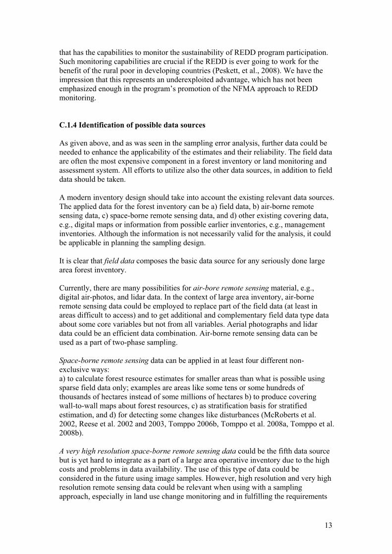
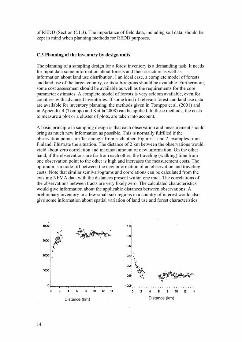
A basic principle in sampling design is that each observation and measurement should

bring as much new information as possible. This is normally fulfilled if the

observation points are 'far enough' from each other. Figures 1 and 2, examples from

Finland, illustrate the situation. The distance of 2 km between the observations would

yield about zero correlation and maximal amount of new information. On the other

hand, if the observations are far from each other, the traveling (walking) time from

one observation point to the other is high and increases the measurement costs. The

optimum is a trade-off between the new information of an observation and traveling

costs. Note that similar semivariograms and correlations can be calculated from the

existing NFMA data with the distances present within one tract. The correlations of

the observations between tracts are very likely zero. The calculated characteristics

would give information about the applicable distances between observations. A

preliminary inventory in a few small sub-regions in a country of interest would also

give some information about spatial variation of land use and forest characteristics.

Distance (km) Distance (km)

15

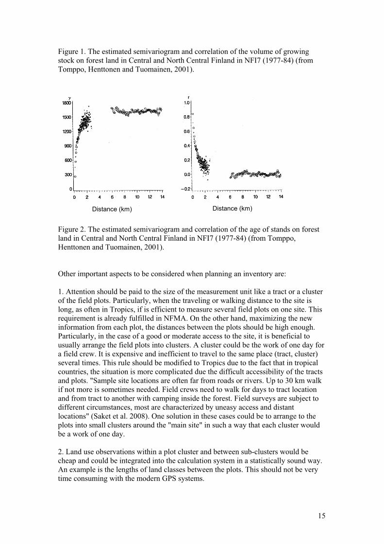
Figure 1. The estimated semivariogram and correlation of the volume of growing

stock on forest land in Central and North Central Finland in NFI7 (1977-84) (from

Tomppo, Henttonen and Tuomainen, 2001).

Distance (km) Distance (km)

Figure 2. The estimated semivariogram and correlation of the age of stands on forest

land in Central and North Central Finland in NFI7 (1977-84) (from Tomppo,

Henttonen and Tuomainen, 2001).

Other important aspects to be considered when planning an inventory are:

1. Attention should be paid to the size of the measurement unit like a tract or a cluster

of the field plots. Particularly, when the traveling or walking distance to the site is

long, as often in Tropics, if is efficient to measure several field plots on one site. This

requirement is already fulfilled in NFMA. On the other hand, maximizing the new

information from each plot, the distances between the plots should be high enough.

Particularly, in the case of a good or moderate access to the site, it is beneficial to

usually arrange the field plots into clusters. A cluster could be the work of one day for

a field crew. It is expensive and inefficient to travel to the same place (tract, cluster)

several times. This rule should be modified to Tropics due to the fact that in tropical

countries, the situation is more complicated due the difficult accessibility of the tracts

and plots. "Sample site locations are often far from roads or rivers. Up to 30 km walk

if not more is sometimes needed. Field crews need to walk for days to tract location

and from tract to another with camping inside the forest. Field surveys are subject to

different circumstances, most are characterized by uneasy access and distant

locations" (Saket et al. 2008). One solution in these cases could be to arrange to the

plots into small clusters around the "main site" in such a way that each cluster would

be a work of one day.

2. Land use observations within a plot cluster and between sub-clusters would be

cheap and could be integrated into the calculation system in a statistically sound way.

An example is the lengths of land classes between the plots. This should not be very

time consuming with the modern GPS systems.

16

2. The size and shape of field plots should be decided and adapted to small scale

variation of forests, or within stand variability of forests when relevant. A further

aspect when planning the size and shape of a plot is the use of ground data with space-

borne remote sensing data. In large area inventories, an efficient plot is usually rather

small due to the fact that within stand variation of forests is small (nearby trees are on

the average more similar than trees far apart from each other). The requirements of

remote sensing and statistical efficiency requirements may be contradicting when

using remote sensing data of medium pixel size like Landsat 5. One should also note

that the use of remote sensing of data is not necessarily technically too complicated

when taking into capacity building plans, and that the coordination of capacity

building and training could suit to FAO.

The small scale variation of forests in Tropics deviates from that in Boreal and

temperate regions and a fairly large size a plot, like NFMA plot, could be argued. In

any case, the plot size and shape could be considered for each country separately. The

size and shape could be selected from a set of some basic alternatives. In the planning

work, some information about the small scale variability of forests is needed. The

forest data of a similar region or a vegetation zone could be one model for the forests.

In addition to the current plot size and shape of NFMA, the basic alternatives are a set

of concentric plots; the radius depends on the breast height diameter of a tree, and an

angle count plot (Bitterlich plot). The radii also depend on the variable in question,

e.g., a shorter radius for dead wood than for living trees.

3. Further stratification on the basis of accessibility could increase the efficiency of an

inventory. The stratification and the estimation can be done in such a way that the

requirements of a sound statistical basis are fulfilled. The basic sample can be made

sparser, e.g., on the basis of needed time (or total costs) to reach a field plot cluster.

The sampling probabilities are applied in the final estimation.

4. As given above, some remote field plots / field plot clusters can be 'measured' on

the basis of air-borne remote sensing. The measurement error should be added to the

total errors. In theory, the measurement errors should be added also for field

measurements, but, the measurement errors are significantly smaller when using field

measurement than when using air-borne data.

One problem in planning the sampling design and plot layout is often the lack the

available data. In some countries, management data could be available for some

regions. One possible data source could the land cover maps based on remote sensing

analysis. Although they include errors, they could be employed in sampling design

planning in a robust way. If some covering digital data are available, the planning of

sampling designs can be done as follows. 1. Potential basic alternatives are identified,

that is, sampling density, the number of the field plots per cluster, the cluster shape,

the distances of the plots in a cluster, the distances between clusters (see, e.g.,

Tomppo 2006a, and Swedish NFI publications). 2. A large amount of samples are

selected using the same design but different 'starting point' (Tomppo et al. 2001,

Tomppo and Katila 2008, Appendix 4). It is sufficient to select some representative

tests areas for sampling simulation from the design units, or alternatively do the

simulation with the country level data. 3. The standard deviation of an estimate

computed from different samples can be considered as a sampling error. On the basis

of the Finnish experiences, this method works very well in practice and has been

17

employed since early 1990s using the output maps of the multi-source NFI. The errors

based on sampling simulations are near the real errors, for error estimation, see, e.g.,

Heikkinen (2006). This approach has been employed in simulating the standard errors

and also the traveling costs in Appendix 4 (Tomppo and Katila 2008).

C.4 Socioeconomic and Institutional Data

In each tract, field crews collect information about forest users and their use of the

resource. These data are collected through a variety of methods, including secondary

data sources (i.e. census data), direct observations (i.e. harvesting activities, cattle

grazing, etc), but principally through different types of interviews with local resource

users themselves. Because of the methodological challenges involved in collecting

high quality of data from interviews, we focus our technical review on these. The

sampling design for the selection of interviewees in each tract is particularly critical

for the quality of data.

The NFMA manual describes three different methods for data collection through

direct interactions with local people: interviews with key informants (i.e. local

individuals with a reputation of being knowledgeable about forest use), focus group

discussions (i.e. meeting with of local resource users to discuss resource use patterns),

and household surveys (i.e. households that are located within a certain distance from

the center of the tract). Seven out of the eight countries that have completed their

assessments rely mostly on information provided by key informants and to some

extent on focus group discussions. For both these forms of interviews, NFMA field

personnel select interviewees through a purposive sampling design. This involves

seeking out individuals whom local people consider to be particularly knowledgeable

about local forest use. Field crews typically rely on qualitative information provided

by local leaders and elders to identify these individuals.

In the cases of Zambia and Kenya, however, NFMA collaborators have added a third

form of interviews: formal household surveys with 16 randomly selected households

within a certain distance from the center of each tract. The NFMA field manual

provides excellent step-by-step instructions for how field personnel should handle the

random selection of these households.

There are several benefits of going beyond interviews with key informants and focus

groups and carrying out household surveys. First, it improves the precision of the

socioeconomic parameter estimates by augmenting the number of observations (that

may be combined to estimate each parameter). These additional data points also help

to provide more reliable interpretations of the data provided by key informants and

focus group discussions (through cross-checking and triangulation). Finally, drawing

data from a suite of different but complementary forms of interviews increases the

confidence in the validity of data. This is particularly important when trying to

measure processes with such high degree of complexity as is the case for forest user

patterns in non-industrialized societies.

Ultimately, the quality of the data collected through these different interviews will

depend on the degree to which these procedures for sampling and interviewing that

are presented in the field manual are actually followed. When it comes to the field

18

application, we note several opportunities for continuing to improve the sampling

design for the interview components of the NFMA program.

We identify four main areas in which the program may improve its performance with

regards to data collection through interviews: (1) Weak links between biophysical

measurements and data gathered though interviews (2) The limitations of relying on

key informants and focus groups alone; (3) Systems for quality control; and (4) The

use of existing data sources in sampling design.

Weak links between biophysical and interview data

One of the fundamental justifications for collecting data through interviews is that this

information is useful for producing policy-relevant knowledge at both the national and

international levels. The idea is that the data on forest users and their relationship to

forests will help policy makers identify priority areas for policy interventions at the

national level. For example, the data may indicate that 30% of the country’s rural

residents do not have secure access rights to fuel wood. The data may also show a

significant correlation between the insecurity of access rights and the degree of forest

degradation. This type of analysis would be extremely valuable for policy analysts

and decision makers.

The problem is that the current NFMA sampling design for interviews limits the

validity of such analytical results because it is difficult to determine the spatial

location of the forest use described by users in interviews. The boundaries of the tract

are perceived as artificial constructs by the interviewee and it is difficult to limit

answers about forest use to this abstract domain. The tenuous links between the

biophysical and socioeconomic data is further weakened by utilizing sampling units

for the two types of data that are of different spatial extents. In Zambia, the difference

in the spatial extent of the sampling unit for socioeconomic data and direct

biophysical measures was about 77.5 km2. The implication is that analysts using the

NFMA data cannot be very sure that the forest use data corresponds to the biophysical

data, and this limits their analytical power.

We propose that the program introduces an additional interview protocol for the focus

group discussions that collects data on ten critical variables related to forest use within

the tract boundaries. By systematically applying this protocol in all field sites,

analysts can be more confident that the socioeconomic data corresponds more closely

to biophysical measurements. We present this protocol in Appendix 1 at the end of the

report.

We also suggest that the program explores more potential measurement synergies

between the biophysical and socioeconomic data collection procedures. For example,

it might be a good idea to have the individuals who responsible for conducting

household interviews to also record GPS points for changing land cover on the

landscape. As per the instructions in the NFMA Field Manual for the selection of

households, field crews are supposed to walk from the center of the tract in direction

of 360˚, 270˚, 180˚, and 90˚, towards the edge of the x km-radius circle. If, after these

four hikes, the crew still has not identified 16 households, they will carry out four

more hikes from the center in the direction of 315˚, 225˚, 135˚, and 45˚. The figure

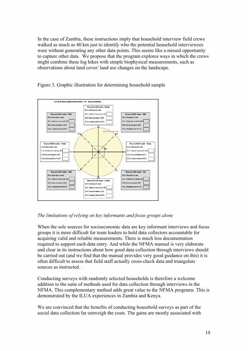
below illustrates these instructions graphically.

19

In the case of Zambia, these instructions imply that household interview field crews

walked as much as 40 km just to identify who the potential household interviewees

were without generating any other data points. This seems like a missed opportunity

to capture other data. We propose that the program explores ways in which the crews

might combine these log hikes with simple biophysical measurements, such as

observations about land cover/ land use changes on the landscape.

Figure 3. Graphic illustration for determining household sample

The limitations of relying on key informants and focus groups alone

When the sole sources for socioeconomic data are key informant interviews and focus

groups it is more difficult for team leaders to hold data collectors accountable for

acquiring valid and reliable measurements. There is much less documentation

required to support each data entry. And while the NFMA manual is very elaborate

and clear in its instructions about how good data collection through interviews should

be carried out (and we find that the manual provides very good guidance on this) it is

often difficult to assess that field staff actually cross-check data and triangulate

sources as instructed. .

Conducting surveys with randomly selected households is therefore a welcome

addition to the suite of methods used for data collection through interviews in the

NFMA. This complementary method adds great value to the NFMA programs. This is

demonstrated by the ILUA experiences in Zambia and Kenya.

We are convinced that the benefits of conducting household surveys as part of the

social data collection far outweigh the costs. The gains are mostly associated with

20

improved reliability of data collection methods (multi-source approach), improved

validity of all social data collected in the site (more independent data to cross-check

and triangulate measures that are particularly difficult to measure) as well as increased

precision in estimating socioeconomic parameters (more observations). Let us take an

example to illustrate this point.

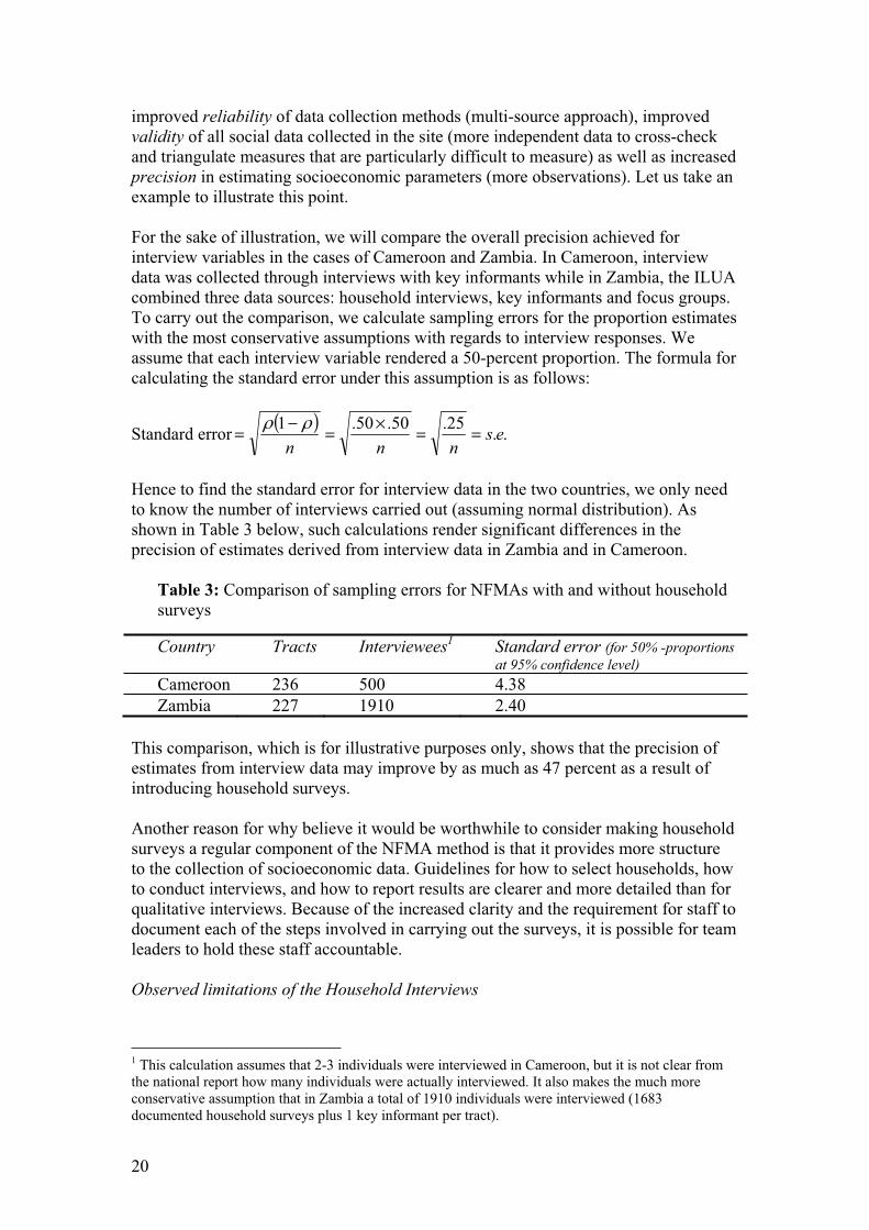
For the sake of illustration, we will compare the overall precision achieved for

interview variables in the cases of Cameroon and Zambia. In Cameroon, interview

data was collected through interviews with key informants while in Zambia, the ILUA

combined three data sources: household interviews, key informants and focus groups.

To carry out the comparison, we calculate sampling errors for the proportion estimates

with the most conservative assumptions with regards to interview responses. We

assume that each interview variable rendered a 50-percent proportion. The formula for

calculating the standard error under this assumption is as follows:

Standard error ..25.50.50.1

esnnn

Hence to find the standard error for interview data in the two countries, we only need

to know the number of interviews carried out (assuming normal distribution). As

shown in Table 3 below, such calculations render significant differences in the

precision of estimates derived from interview data in Zambia and in Cameroon.

Table 3: Comparison of sampling errors for NFMAs with and without household

surveys

This comparison, which is for illustrative purposes only, shows that the precision of

estimates from interview data may improve by as much as 47 percent as a result of

introducing household surveys.

Another reason for why believe it would be worthwhile to consider making household

surveys a regular component of the NFMA method is that it provides more structure

to the collection of socioeconomic data. Guidelines for how to select households, how

to conduct interviews, and how to report results are clearer and more detailed than for

qualitative interviews. Because of the increased clarity and the requirement for staff to

document each of the steps involved in carrying out the surveys, it is possible for team

leaders to hold these staff accountable.

Observed limitations of the Household Interviews

1 This calculation assumes that 2-3 individuals were interviewed in Cameroon, but it is not clear from

the national report how many individuals were actually interviewed. It also makes the much more

conservative assumption that in Zambia a total of 1910 individuals were interviewed (1683

documented household surveys plus 1 key informant per tract).

Country Tracts Interviewees1

Standard error (for 50% -proportions

at 95% confidence level)

Cameroon 236 500 4.38

Zambia 227 1910 2.40

21

The NFMA approach to household interviews does, however, face several constraints.

Some of the perceived limitations of the household interviews include (a) difficulties

in communicating the true meaning of questions to interviewees; (b) the large number

of questions in each interview, and (c) difficulties in assessing the represenattaiveness

of the observations. What follows is a short discussion on how these limitations might

be addressed.

(a) Difficulties in communicating the true meaning of questions

If a question is perceived as complex, and interviewees have trouble understanding its

meaning, we recommend that the question is dropped from the interview protocol

because the question will render highly unreliable responses. One way of addressing

problematic questions is to invest more in field testing before the NFMA is carried out.

During this phase, interviewers document which are the most difficult questions. After

identifying these, the team of interviewers can discuss ways of simplifying or

otherwise modifying the wordings. This same exercise should be carried out at the

end of each NFMA and ILUA so that future NFMAs in other countries may benefit

from the lessons learned in previous countries’ interview experiences. It would be

particularly important to capture the more experienced field crews’ expert knowledge

of how one might rephrase questions to improve on clarity.

(b) Large number of questions.

The large number of questions means that household interviews may take

considerable time to complete. Interview crews in Zambia reported that in some cases

one household interview tool as long as 1.5 - 2 hours to complete. A large share of

interview questions concern products and services. Interviewees ask for a complete

inventory of all products and services used by each household. These questions are

identical to questions asked to key informants and focus groups. One way of reducing

the time spent in each household would be focus questions on the three most

important products and services rather than asking question about the full set.

While there may be an excess of detail when it comes to certain sets of questions, it is

surprising to note the complete absence of other potentially very important questions.

For example, in the available data from household surveys from Zambia, we were

unable to identify data collected on variables such as the level of schooling in each

household; personal health indicators; degree of direct dependence on forest resources

for the household’s economy; access to public services—such as health services,

primary education, and forestry extension services or other forestry-related personnel

from external organizations, as well as estimates of the total number of households in

each tract. The analysis using household data from Zambia, presented in Appendix 2,

was complicated by the absence of such variables because existing analytical work on

forestry policy refer to these variables as potentially influential.

(c) Difficulties in assessing the representativeness of the observations

The NFMA team has expressed some concern over the difficulties in assessing the

representativeness of household interview data at the tract and provincial levels. Much

of this problem is related to the fact that the total number of households is not a piece

of data that is collected in each tract. This is a critical variable to collect data on

because when populations are small, the size of the sample becomes critical for

estimating representativeness.

22

Systems for quality control

No matter how detailed the instructions in the field manual and no matter how

competent the field staff is, there are no guarantees that all data will be collected

according to the established protocol. While it is important to monitor field crews and

periodically check the quality of their work, it is often more effective to create quality

control systems that reward good performance rather than punishing staff for the

opposite.

Such a reward system may involve offering incentive payments to field teams that

provide exceptionally well-documented support for the coded data collected through

interviews. Such documentation may be in the form of photographs with interviewed

individuals and groups, materials from Participatory Rural Appraisal exercises, and

maps that mark observations made during transect walks with user group

representatives. Simply asking questions to interviewers about why they have coded

information in a certain way is often sufficient for team leaders to get a sense of the

level of rigor that the they applied to collect and interpret the data.

Ultimately, much of the quality of the data depends on the relationship between team

leaders and the individuals responsible for data collection. No system of control,

punishment, or rewards can compensate for a breakdown in this crucial relationship.

The use of existing data sources in sampling design

Just as the precision of NFMA field measurements may be improved by relying on

existing land cover data for the sampling design, so can the efficiency of data

collection through interviews be improved by building on existing or planned efforts

of data collection in the country in question.

For example, in some countries it may be possible to join forces with organizations

that have carried out (or plan to) national household surveys, i.e. population census,

agricultural census or World Bank-supported Poverty and Vulnerability Assessments

(PVA). In the case of the ILUA program in Zambia, a PVA was carried out in 2005,

which coincided partially with the data collection for the ILUA in Zambia, but the two

programs collected their household data independently and with different designs.

In some cases, it may be of mutual benefit to seek compatibility between survey

systems of other organizations or to agree on a future design that is acceptable to both

NFMA and partner organizations. The gains of seeking out such synergies are not

limited to the increased precision of estimates but it also makes it possible to link the

NFMA data to issues that are normally beyond the scope the typical NFMA program.

23

D. STATISTICAL FRAMEWORK

This section reviews the statistical framework of the NFMA programs. We focus our

review on how the national components make use of statistical inference to learn

about the state of their country’s forest resources and how these are being used by

local people. For this, we examined the national reports of Bangladesh, Cameroon,

Guatemala, Honduras, Lebanon, Philippines, and Zambia.

D.1 Biophysical calculations

In result calculations, basic estimators of ratio estimation and stratified ratio

estimation have been employed with equal inclusion probabilities for the expected

values and variances. The independence of the observations has been assumed. The

given formulas are correct and very likely correctly used.

In error estimation, the observation of one tract (i.e., from the plots in a tract) has been

merged into one observation. This is also our recommendation due to the closeness of

the plots. Underestimates of the error estimates will be obtained if the variables on the

observation units are spatially correlated and are assumed to be independent in the

estimators. There are some studies showing that spatial correlation of mean volume of

growing stock or the number of the species is quite low even at low distances in

Tropical rain forests (e.g. Singh 1974). The spatial correlation of land classes often

deviates from that of volume and tree species distributions. Keeping in mind that the

inventories should also produce the estimates of land class areas, the spatial

correlation of different variables needs further and country specific investigations.

Our first comment related to NFMA results calculation is that fact that, in practice, the

inclusion probabilities vary in latitude longitude sampling with increasing inclusion

probabilities towards North and South from the Equator. This leads overweighting of

the observations measured at locations further away from the equator relative to

observations measured closer to the equator. The seriousness this problem depends on

how far the target country is from the equator. We encourage checking one more time

the analysis in this respect. The problem could be overcome by attaching varying

inclusion probability (area representativeness or plot expansion factor) into each plot

and tract, and therefore does not constitute a major problem. The area represented by

each plot could be derived, e.g., from the areas of the four nearest rectangles restricted

by the latitudes and longitudes, or using the areas of Voronoi cells as the weights of

the plot clusters. Voronoi cells are made up of polygons which are created around

geographical entities, such as spatially distributed object points, e.g., trees or plot

centers, and a closeness principle. Each polygon contains those points of the space

which are closer to that specific object point than any other point (Voronoi 1908).

Our second comment concerns the use of the possible other existing data or remote

sensing data. The efficiency could be increased with minor costs when using either

post-stratification or small area estimation.

Forest inventory and statistical textbooks involve large amount information about

statistical inference relevant for statistical analysis. The principles given in the books

give good basis for statistical guidelines. In addition to what the books give, we would

like to emphasize the following points:

24

Three types of estimates can be seen from the entire NFI system:

1. Large area estimates and error estimates based on field data only. This group

includes also the change estimates. Note that a part of 'field data' could come from air-

borne remote sensing. The estimates should be computed by strata. The stratum-wise

estimates and error estimates can be considered independent which makes it trivial to

merge stratum-wise estimates to nation level estimates. Post-stratified estimation

within the basic strata can be done if suitable data are available, e.g., the old

management data or new maps based on multi-source inventory (field data and space-

borne remote sensing). This method would increase the efficiency of the field data

with small additional costs (McRoberts et al 2002, Nilsson et al. 2007).

2. Multi-source estimates, i.e. statistics for small areas, can be calculated using field

data, space-borne remote sensing data and other available data (Reese et al, 2003,

Tomppo, 1992, Tomppo and Halme, 2004, Tomppo 2006b, Tomppo et al. 2008a and

2008b).

3. Map form predictions of core forest variables based on all available data, i.e., field

data supported by air-borne remote sensing data, space-borne remote sensing and

other digital data. Map form estimates can be derived also from field data only.

Furthermore, we would like to emphasis on the following points.

4. It is important to have error estimates for all parameters.

5. The result calculation principles, possibly with the calculation formulas should

always be given in the reports. This is important not only for the users but for the

wider audience to increase the trust.

D.2 Socioeconomic data analysis

For the analysis of socioeconomic data we pay particular attention to the national

teams’ treatment of uncertainty and the extent to which the reports discuss the

implications of limited accuracy and precision of the interview data.

Analysis of Uncertainty

One of the fundamental rules in the analysis of interview or survey data is the explicit

calculation and discussion of the level of uncertainty generated by data collection and

estimation processes. There are two major sources of uncertainty that should be

addressed in any analysis of informant based on interviews: namely sampling error

and measurement error. All the NFMA country reports that we reviewed for this

report presented results from interview data, in both tables and diagrams, but none of

them sampling and measurement errors into account. This can be very misleading to

readers. .

By including estimations of different types of error—based on the number of

interviewees, the way they were selected, their respective interests in relation to forest

25

use, and the informants’ social and economic positions—a more robust interpretation

of the interview data is be possible.

Sampling error

For forest mensuration data collected, it is relatively straightforward to calculate valid

estimates of variance, standard deviations, and thereby confidence intervals for these

continuous variables. For interview data, however, some unique problems arise when

estimating sampling error. The problems are due to the nature of the variables

measured, which are either binary (values are either 0 or 1), ordinal (values represent

order of importance or rank, or nominal (categories without any particular ordering

properties). Such categorical variables contain less variance, because measurements

are fit into predetermined categories. And due to the non-continuous nature of such

variables, special statistical techniques need to be employed when calculating

sampling error for categorical data.

Simply put, sampling error is the difference between the sample estimate and the

corresponding population’s true parameter value. Using conventional (parametric)

statistical techniques to calculate the sampling error for any given measure requires

that the sample is normally distributed (bell-shaped distribution curve). But when you

have data that consists mostly of 0 and 1, it is not self-evident what a normal

distribution looks like. In this, researchers often make assumptions about the

distribution based on how the sample was drawn. Random and systematic sample

designs are known to generate normal distributions for all types of data.

Since FAO’s NFMA follows a systematic sample strategy one might be tempted to

conclude that interview data is always normally distributed. This is not always true,

because the degree of normality will ultimately depend on how interviewees were

selected in each tract. In the cases in which randomly selected households are

interviewed in each systematically selected tract (such as the case of Zambia and

Kenya), the normality assumption will hold. But for interview data using more

qualitative selection procedures (interviewing key informants and focus groups) the

data may or may not meet the normality criterion. To maintain normality in these

cases, it is important to follow an identical procedure for identifying interviewees in

each site. Such procedures are described in the FAO NFMA Manual as well as in the

FAO-IUFRO Knowledge Reference.

Assuming normality, it is possible to calculate the precision of particular measures

and estimates of the interview data. Consider the following example: For a 95-

percent confidence interval and for questions where the sampled interviewees’

answers were split down the middle (50 % answering “yes” and the other 50%

answering “no”, which is the most conservative estimate for calculating interview

sampling error) the sampling error for a sample of 260 interviews produces an

estimated sampling error of 6.8%. For questions where a smaller or larger proportion

responded affirmatively the sampling error will be even smaller. Illustration 1 below

offers an example of how sampling error may be calculated for categorical variables

from NFMA interview data. Reporting on such errors in relation to particular

estimates in the results should be standard procedure for all NFMA reports.

It is considered good practice to account for the degree of precision when presenting

any analytical results derived from a sample. All NFMA reports should therefore

26

make it a habit to present sampling errors for all quantitative variables reported,

regardless of whether these measure socio-economic or biophysical phenomena. But

sampling error is only one component of the total measure of uncertainty in a given

result. There are other types of errors that are important sources of uncertainty in the

NFMA. Measurement error is of particular concern for the NFMA interview

component and the next section discusses how this type of error may be accounted in

the reporting.

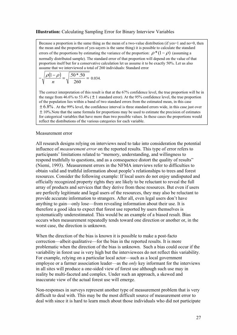
27

Illustration: Calculating Sampling Error for Binary Interview Variables

Measurement error

All research designs relying on interviews need to take into consideration the potential

influence of measurement error on the reported results. This type of error refers to

participants’ limitations related to “memory, understanding, and willingness to

respond truthfully to questions, and as a consequence distort the quality of results”

(Niemi, 1993). Measurement errors in the NFMA interviews refer to difficulties to

obtain valid and truthful information about people’s relationships to trees and forest

resources. Consider the following example: If local users do not enjoy undisputed and

officially recognized property rights they are likely to be reluctant to reveal the full

array of products and services that they derive from these resources. But even if users

are perfectly legitimate and legal users of the resources, they may also be reluctant to

provide accurate information to strangers. After all, even legal users don’t have

anything to gain—only lose—from revealing information about their use. It is

therefore a good idea to expect that forest use reported by users themselves is

systematically underestimated. This would be an example of a biased result. Bias

occurs when measurement repeatedly tends toward one direction or another or, in the

worst case, the direction is unknown.

When the direction of the bias is known it is possible to make a post-facto

correction—albeit qualitative—for the bias in the reported results. It is more

problematic when the direction of the bias is unknown. Such a bias could occur if the

variability in forest use is very high but the interviewees do not reflect this variability.

For example, relying on a particular local actor—such as a local government

employee or a farmer association leader—as the only key informant for the interviews

in all sites will produce a one-sided view of forest use although such use may in

reality be multi-faceted and complex. Under such an approach, a skewed and

inaccurate view of the actual forest use will emerge.

Non-responses in surveys represent another type of measurement problem that is very

difficult to deal with. This may be the most difficult source of measurement error to

deal with since it is hard to learn much about those individuals who did not participate

Because a proportion is the same thing as the mean of a two-value distribution (if yes=1 and no=0, then

the mean and the proportion of yes-sayers is the same thing) it is possible to calculate the standard

errors of the proportions by estimating the variance of the proportion: )1(* (assuming a

normally distributed sample). The standard error of that proportion will depend on the value of that

proportion itself but for a conservative calculation let us assume it to be exactly 50%. Let us also

assume that we interviewed a total of 260 individuals: Standard error

=260

50.*50.1

n0.034.

The correct interpretation of this result is that at the 67% confidence level, the true proportion will be in

the range from 46.6% to 53.4% ( 1 standard error). At the 95% confidence level, the true proportion

of the population lies within a band of two standard errors from the estimated mean, in this case

%8.6 . At the 99% level, the confidence interval is three standard errors wide, in this case just over

10%.Note that the same formula for proportions may be used to estimate the precision of estimates

for categorical variables that have more than two possible values. In these cases the proportions would

reflect the distributions of the various categories for each variable.

28

in interviews (Fowler, 1993). In the NFMA interviews, field crews are under a great

deal of pressure to finish their fieldwork on time. If one of the pre-selected

interviewees is not available or refuses to be interviewed, field personnel will select

an alternate interviewee without necessarily recording that the person who was pre-

selected could not participate. Consequently, the NFMA interview sample is likely to

be systematically biased towards those individuals who have more time to talk, and

who have less to lose from divulging information about their forest use. We strongly

advise the NFMA to incorporate non-responses in the field protocols so that NFMA

teams may estimate its influence on total uncertainty of sample estimates.

Another potential source of inaccuracy is the respondent’s hidden agenda with regards

to local forest use. Interviewees may deliberately conceal or distort information even

if they do not have an apparent reason to do so. Without proper triangulation and

cross checking of responses such inaccuracies are virtually impossible to detect.

Utilizing a multi-source approach, which includes a suite of methods for data

collection on socioeconomic data will contribute to more accurate data because with

more sources of different types you increase your ability to assess the validity of

interview responses.

All these measurement problems affect the accuracy of the sample estimates. The crux

of it is that unlike sampling error, it is not possible to calculate the precise size of the

measurement error. That does not mean that it should not be addressed in the reports.

What it does mean is that reports need to discuss the influence measurement error in

more qualitative terms by addressing a series of key issues. Some of these issues

include how interviewees were selected, how many individual interviews were carried

out, if and how interviewers were trained, if and how interview instruments were pre-

tested and validated, among others.

The FAO-IUFRO Knowledge Reference for National Forest Assessments describes a

basic approach for how interviewees should be identified. According to the FAO-

IUFRO-recommended approach, measurement error may be partly mitigated by

selecting interviewees according to their interests in the tree-related products and

services. By interviewing the widest variety of local actors possible—with respect to

their different interests in products and services—the sample estimates will be less

biased. Since it is not possible to calculate this bias in any mathematically exact way,

the NFMA teams should describe the detailed measures taken to address measurement

error. Doing so will enhance the transparency of the research, as well as adding to the

credibility of the results presented. The illustration below outlines a series of steps

that the NFMA teams are advised to follow when analyzing and presenting the NFMA

interview results. This is information that the readers need for proper interpretation of

the results.

29

Illustration: Addressing Measurement Error for Interview Variables

E: CONCLUSIONS AND RECOMMENDATIONS

As external reviewers we find that FAO’s support to NFMA has been extremely

important in meeting member countries’ and partner organizations’ demands for more

and better data about forests and their users. We believe this program has done more

for the improvement of the quality of globally available forest data that any other

program that we have been in contact with.

At the same time, because of its innovative orientation, ambitious scope, and

relatively short history, we believe it is of utmost importance to reflect on how things

may be done even better. Only with a keen sensitivity for how to adapt to the

changing conditions and shifting demands will a program like this one be able to

maintain its steadfast leadership. Adaptation requires learning and experimenting with

ways of doing things even better. Our recommendations should be viewed as our

input into this continuous learning process.

1. Explore alternative sampling designs and plot lay-outs. Our related sampling

simulation study in Appendix 4 shows that the NFMA design is not as efficient for

estimating biophysical parameters as the tested alternative designs. One of our

most important recommendations is that the program should seriously reconsider

promoting a blue-print sampling design because what is cost-effective data

collection in one country will not be the same in all countries. Needs for accuracy,

scope, and emphasis are different from country to country. The availability of

existing data varies from country to country, and as we have shown, the cost-

effectiveness of any sampling design depends is largely determined by how

effective the design is in employing the existing data.

We find that the current plot layout is time consuming and similar trees are

measured again and again. Our preliminary analysis suggests that one would be

able to generate more or less the same level of precision for estimates of biomass

volumes even if one measured one third as many trees as is currently done in the

NFMA.

2. Promote experimentation and pilot studies to learn how the NFMA design

may be made even better. Encouraging countries to experiment with alternative

Diagnostic questions for assessing measurement error in interviews:

1. How was the interview instrument developed?

2. How many field tests were carried out?

3. What was the result of the field test?

4. Who carried out the interviews?

5. What training did the interviewers go through?

6. How were interviewees identified and selected?

7. How many interviewees were interviewed in total?

8. Did the number of interviewees vary form one tract to another? Why?

30

designs and then comparing results with other experiences will enrich all NFMA

participants. Pilot studies on new ways of doing things may lead to more efficient

designs for responding to specific needs of different member countries. One area

in which the program should invest in such experimentation is for national forest

carbon accounting related to participation in UNFCCC REDD initiative. Another

urgent topic for a pilot study would be “appropriate design and methods for

estimating over-time changes in forest parameters” utilizing data from NFMAs

that have been carried out more than once (which will hopefully occur very soon).

3. Continue promoting the collection of socioeconomic and institutional data

through interviews as part of the NFMA approach. It is not only a defining

characteristic of this program, but it also provides much needed data on potential

causes for observed variation in forest measurements. Hence it helps policy

makers to understand the reasons for why forest conditions vary across space and

time. But perhaps more importantly, it is data from this component that will allow

us to test the effectiveness of policy and varying governance arrangements at local

and national levels to induce sustainable use of forests. All of these wonderful

potential benefits, for a relatively meager marginal cost.

4. Strengthen the links between biophysical field measurements and data

gathered though interviews. We propose that the program introduces an

additional interview protocol for the focus group discussions that collects data on

ten critical variables related to forest use within the tract boundaries. By

systematically applying this protocol in all field sites, analysts can be more

confident that the socioeconomic data corresponds more closely to biophysical

measurements (see appendix 1).

We also suggest that the program explores more potential measurement synergies

between the biophysical and socioeconomic data collection procedures. For

example, it might be a good idea to have the individuals who responsible for

conducting household interviews to also record GPS points for changing land

cover on the landscape, as they walk from one household to the next. The

interview crews cover great distances by foot when identifying the household

sampling units and could potentially combine these hikes with simple biophysical

measurements.

5. Establish surveys with randomly selected households as the core of a “multi-

source” approach to socioeconomic and institutional data collection. We are

convinced that the benefits of conducting household surveys as part of the social

data collection far outweigh the costs. The gains are mostly associated with

improved reliability of data collection methods (multi-source approach), improved

validity of all social data collected in the site (more independent data to cross-

check and triangulate measures that are particularly difficult to measure) as well

as increased precision in estimating socioeconomic parameters (more

observations).

6. Invest in quality control systems that reward good interview performance No

matter how detailed the instructions in the field manual and no matter how

competent the field staff is, there are no guarantees that all data will be collected

31

according to the established protocol. Some countries seem to have been more

rigorous than others in introducing systems for quality control. We recommend

that the lead agency in each country follows the example of Guatemala, Honduras

and Nicaragua; and conducts routine controls with in-situ re-measurements to

ensure compliance by the field crews. While it is important to monitor field crews

and periodically check the quality of their work, it is often more effective to create

quality control systems that reward good performance rather than punishing staff

for the opposite.

7. Exploit opportunities to use existing data sources in sampling design. There

are opportunities to make better systematic use of remote sensing data on land

cover and land use to improve cost-effectiveness of design and statistical

framework. It is important to note, however that such incorporations should not

come at the cost of fieldwork, but should be seen as a complement to field

measurements. It is an emerging consensus in the forest inventory science

community that by combining remote sensing and field measurements one is in a

position to learn as much as ten times as much as compared to relying exclusively

on one source or the other (provide examples from experiences in US, Sweden,

Finland). All countries applying NFMAs would benefit from integration of RS

data in the sampling design stage of the NFMA. We recommend that the RS and

field analyses be carried out in an integrated fashion by one and the same agency.

The RS component should not be outsourced because this would jeopardize some

of the synergy effects.

Similar opportunities exist to make the sampling design for the interview

component more efficient. The efficiency of data collection through interviews

may be improved by building on existing or planned efforts of data collection in

the country in question. For example, in some countries it may be possible to join

forces with organizations that have carried out (or plan to) national household

surveys, i.e. population census, agricultural census or World Bank-supported

Poverty and Vulnerability Assessments (PVA).

8. Invest more in analysis. Although this review has focused on the methodological

considerations involved in the organization of data collection, we cannot end this

review without urging that more emphasis to be given to the need for more and

better analysis of all NFMA data. There is an incredible wealth of data available,

but so far very little of it has been utilized in scientific studies. We propose that

system is created that makes some version of the data-sets (without coordinates)

accessible to interested and respectable members of the research community. We

are convinced that having more scientists using this data would not only deliver

more knowledge to the interested parties, but it would also augment the program’s

visibility. Ideally, the analysis should be carried out by the in-country colleagues

together with other analysts. Supporting training opportunities for NFMA

colleagues to continue to develop their analytical skills seems like a crucial part of

such an endeavor.

33

REFERENCES

Andersson, K. and Svendsen, S. 2006. Analyzing Interview Data from the National

Forest Assessments. FAO-NFMA Working Paper # 4. Rome, Italy: The Food

and Agriculture Organization of the United Nations.

Armor, D.J. 1974. Theta Reliability and Factor Scaling. In H.L. Costner (ed.)

Sociological Methodology 1973-1974, pp 17-50. San Francisco: Jossey-Bass.

Blalock, H. M. Jr. 1972. Social Statistics. New York, NY: McCraw-Hill Companies.

Bohrstedt, G. W. 1970. Reliability and Validity Assessment in Attitude Measurement.

In G. F. Summers (ed.) Attitude Management, pp- 80-99. Chicago, IL: Rand

McNally .

Branthomme, A. 2002. Field Manual: Cameroon National Forest Inventory. Rome,

Italy: FAO.

Cienciala, E., Tomppo, E., Snorrason, A., Broadmeadow, M., Colin, A., Dunger, K.,

Exnerova, Z., Lasserre, B., Petersson, H., Priwitzer, T., Sanchez, G. & Ståhl,

G. 2008. Preparing emission reporting from forests: use of National Forest

Inventories in European countries. Silva Fennica 42(1): 73-88.

Czaplewski, Raymond L. 2003. Chapter 5: Accuracy assessment of maps of forest condition: statistical design and methodological considerations, pp. 115-140. Remote Sensing of Forest Environments: Concepts and Case Studies. (Michael A. Wulder and Steven E. Franklin, Eds.) Kluwer Academic Publishers, Boston. 515p.

Czaplewski, R.L., McRoberts, R.E., Tomppo, E. 2004. Sample design. In: Andersson,K, Bhandari, N., Czaplewski, R., Hussin, Y., Janz, K., Kleinn, Ch., Magnussen, S. McRoberts, R. Melin, Y. Persson, R. Reed, D. Sandewall, M., Ståhl, G., Thomson, A., Tomppo, E., Vanclay, J. Knowledge Reference for National Forest Assessments. http://www.fao.org/forestry/NfaKnowledgeRef/en/

Cronbach, L.J. 1951. Coefficient Alpha and the Internal Structure of Tests.

Psychometrika, 16, pp. 297-334.

FAO 2002. Final report Kotka IV: Expert consultation on Global Forest Resources

Assessments – Linking National and International efforts. Kotka, Finland , 1-5

July 2002.

FAO, 2001. Committee on Forestry 2001 (COFO 2001). Proceedings. Rome, Italy:

FAO

Fowlern, F. J. 1988. Survey Research Methods. Newbury Park, CA: Sage

Publications.

Gregoire, T.G. and Valentine, H.T. 2007. Sampling Strategies for Natural Resources

and the Environment. 474 p. Chapman & Hall.

Govil, K. 2002. The Conceptual Frameworks for Identification, Assessment and

Aggregation of Global Variables and Criteria for Global Forest Resources

Assessment. Paper presented at the FRA Advisory Board 1st meeting. Nairobi,

Kenya, 16-18 October, 2002.

Gujarati, D. N. 1995. Basic Econometrics. New York, NY: McGraw-Hill Book

Company.

Hauser, P. 1969. Comments on Coleman’s Paper. In. R. Bierstedt (ed) A Design for

Sociology: Scope Objectives and Methods. pp.122-36. Philadelphia, PA:

American Academy of Political and Social Science.

Heikkinen J (2006) Assessment of uncertainty in spatially systematic sampling. In:

A. Kangas A, Maltamo M (ed) Forest Inventory - Methodology and

34

Applications, Managing Forest Ecosystems Vol. 10. Springer, Dodrecht, The

Netherlands pp. 155-176.

Homer-Dixon, T. F. 1999. Environment, Scarcity, and Violence. Princeton, N.J.:

Princeton University Press.

Intergovernmental Panel on Forests. 1997. Proceedings from the 4th Session. New

York, NY: United Nations: ECOSOC..

Katila M (2006b) Empirical errors of small area estimates from the multisource

National Forest Inventory in Eastern Finland. Silva Fenn 40:729-742

Katila M, Heikkinen J, Tomppo E (2000) Calibration of small-area estimates for map

errors in multisource forest inventory. Can J For Res 30:1329-1339

Katila M, Tomppo E, (2001) Selecting estimation parameters for the Finnish multi-

source national forest inventory. Remote Sens. Environ 76:16-32

Katila M, Tomppo E. 2002. Stratification by ancillary data in multisource forest

inventories employing k-nearest neighbour estimation. Can J For Res 32(9):

1548-1561.

Kim H-J, Tomppo E (2006) Model-based prediction error uncertainty estimation for

k-nn method. Remote Sens of Environ 104:257-263

King, G., R. O. Keohane and S. Verba. 1994. Designing Social Inquiry: Scientific

Inference in Qualitative Research. Princeton, NJ: Princeton U. Press.

Klein, C., C. Ramirez, G. Chavez and S. Lobo. 2000. Pilot forest inventory in Costa

Rica. Report to FAO FRA. Rome, Italy: FAO.

Lansing, J. B. and J. N. Morgan. 1971. Economic Survey Methods. Ann Arbor, MI:

Institute for Social Research, University of Michigan.

Lasswell, H. 1958. Politics: Who gets What, When and How. New York, NY:

Meridian Books.

Magnussen S, McRoberts RE, Tomppo E (2008) A model-based estimator of the

mean square error of k-nearest neighbour predictions with remotely-sensed

ancillary variables. Remote Sens of Environ. in Press.

Mandallaz. D. 2008. Sampling Techniques for Forest Inventories. Chapman & Hall

(CRC Press). 272 p.

McRoberts RE, and Tomppo EO, 2007. Remote sensing support for national forest

inventories. Remote Sens of Environ 110: 412-419

McRoberts RE, Nelson MD and Wendt DG (2002a) Stratified estimation of forest

area using satellite imagery, inventory data, and the k-Nearest Neighbors

technique. Remote Sens of Environ 82:457-468

McRoberts RE, Tomppo EO, Finley AO, Heikkinen J 2007. Estimating areal means

and variances of forest attributes using the k-Nearest Neighbors technique and

satellite imagery. Remote Sens of Environ 111: 466-480

McRoberts RE, Wendt DG, Nelson MD and Hansen MH (2002b) Using a land cover

classification based on satellite imagery to improve the precision of forest

inventory area estimates. Remote Sens of Environmen 81:36-44

Moser, C. O. N. (1989) ‘Gender Planning in the Third World: Meeting Practical and

Strategic Gender Needs’, World Development, 17 (1): 1799-1825.

Niemi, I. 1993. Systematic error in behavioral measurement: Comparing results from

interview and time budget studies. Social Indicators Research 30(2-3):229-

244

Novick, M. and C. Lewis, 1967. Coefficient Aloha and the Reliability of Composite

Measurements. Psychometrika, 32, pp 1-13.

35

Nilsson, M. 1997, Estimation of Forest Variables Using Satellite Image Data and

Airborne Lidar. Doctoral thesis. Swedish University of Agricultural Sciences,

Umeå.

Nunnally, J. C. 1967. Psychometric Theory. New York, NY: McGraw- Hill Book

Company.

Ostrom, E. (1999). Self-Governance and Forest Resources. Occasional Paper No. 20

(February). CIFOR. Bogor, Indonesia, Center for International Forestry

Research: 1-15.

Parten, M. 1950. Surveys, Polls, and Samples: Practical Procedures. New York, NY:

Harper and Brothers, Publishers.

Persson, R. and K. Janz (2004). Rationale - Policy influence. In Knowledge Reference

for National Forest Assessments. Rome: FAO

Peskett, L. Huberman, D. Bowen-Jones, E. Edwards, G. Brown, J. 2008. Making

REDD work for the poor. Poverty Environment Partnership (PEP).

Picciotto, R. and E. Wiesner. 1998. Evaluation & Development: The Institutional

Dimension. Washington, DC: The World Bank.

Pindyck, R. S. and D. L. Rubinfeld. 1981. Econometric Models and Economic

Forecasts. New York, NY: McGraw-Hill Book Company.

Ramirez, C. and R. Rodas. 2002. Manual de Campo: Inventario Forestal Nacional de

Guatemala. Rome, Italy: FAO.

Ranneby, B. 1985. Designing a new national forest survey for the Heilongjiang

Province. Unpublished report. Project CPR/82/010, FAO. Rome

Reese H, Nilsson M, Granqvist Pahlén T, Hagner O, Joyce S, Tingelöf U, Egberth M,

Olsson H (2003) Countrywide estimates of forest variables using satellite data

and field data from the National Forest Inventory. Ambio 32:542-548

Reese H, Nilsson M, Sandström P, Olsson H (2002) Applications using estimates of

forest parameters derived from satellite and forest inventory data. Comput and

Electron in Agric 37:37-56

Repetto, R.C and M. Gillis. 1988. Public Policies and the Misuse of Forest Resources.

New York: Cambridge University Press

Rojas, M. 1989. Women in community forestry: a field guide for project design and

implementation. Community Forestry Guidelines 1. Rome: FAO

Rossi, P. H., J. D. Wright and A.B. Anderson. 1983. Handbook of Survey Research.

San Diego, CA: Academic Press, Harcourt Brace Jovanovich.

Saket, M, D. Altrell, A, Branthomme and P. Vuorinen. 2002. FAO’s Approach to

support for national forest assessments for Country Capacity Building. Paper

presented at the FAO Expert Consultation “KOTKA IV” in Kotka, Finland,

July 1-5, 2002.

Saket, M. 2002. Forestry and tree information gaps at national level. Paper presented

at the FAO Expert Consultation “KOTKA IV” in Kotka, Finland, July 1-5,

2002.

Saket, M., Altrell, D., Branthomme, A., Kim, H-K., Leppänen, M.,. Piazza, M. and K

Tavani, R., 2008. Comments on The Technical Review of FAO’s Approach

and Methods for National Forest Monitoring and Assessment (NFMA) by

Erkki Tomppo and Krister Andersson. Unpublished report. FAO.

Singh, K.D. 1974. Spatial variation in the Tropical Rain Forests. Unasylva. 106. Vol

26.

Stevens, S. S. 1968. Measurement, Statistics and the Schemapiric View. Science, 161:

849-56.

36

Thomson, J. T. 1992. A Framework for Analyzing Institutional Incentives in

Community Forestry. Community Forestry Note No. 10. Rome, Italy: FAO.

Tomppo E (1991) Satellite Image-Based National Forest Inventory of Finland. In:

Proceedings of the symposium on Global and Environmental Monitoring,

Techniques and Impacts, September 17-21, 1990 Victoria, British Columbia

Canada. International Archives of Photogrammetry and Remote Sens 28:419-

424

Tomppo E (2006a) The Finnish National Forest Inventory. In: Kangas A., Maltamo M

(ed) Forest inventory. Methodology and applications, Managing Forest

Ecosystems Vol 10. Springer, Dordrecht, The Netherlands pp. 179-194

Tomppo E (2006b) The finnish multi-source national forest inventory - small area

estimation and map production. In: Kangas A., Maltamo M (ed) Forest

inventory. Methodology and applications, Managing Forest Ecosystems Vol

10. Springer, Dordrecht, The Netherlands pp. 195-224

Tomppo, E., Henttonen, H., Korhonen, K.T., Aarnio, A., Ahola, A., Heikkinen, J., Ihalainen, A., Mikkelä, H., Tonteri, T. and Tuomainen, T. 1998. Etelä-Pohjanmaan metsäkeskuksen alueen metsävarat ja niiden kehitys 1968-97. (Forest Resources and their development in Forestry Board Centre 'Etelä-Pohjanmaa in 1968-97, in Finnish). Folia Forestalia 2B/199: 293-374.

Tomppo E, Henttonen H, Tuomainen T (2001b) Valtakunnan metsien 8. inventoinnin

menetelmä ja tulokset metsäkeskuksittain Pohjois-Suomessa 1992-94 sekä

tulokset Etelä-Suomessa 1986-92 ja koko maassa 1986-94. Folia For

1B/2001:99-248 (In Finnish).

Tomppo E, Halme M (2004) Using coarse scale forest variables as ancillary

information and weighting of variables in k-nn estimation: a genetic algorithm

approach. Remote Sens. Environ. 92:1-20

Tomppo E, Korhonen KT, Heikkinen J, Yli-Kojola H (2001a) Multisource inventory

of the forests of the Hebei Forestry Bureau, Heilongjiang, China. Silva Fenn

35(3):309-328

Tomppo E, Olsson H, Ståhl G, Nilsson M, Hagner O and Katila M (2008a).

Combining National Forest Inventory Field Plots and Remote Sensing Data

for Forest Databases. Remote Sensing of Environ 10.1016/j.rse.2007.03.032.

Tomppo, E., Haakana, M., Katila, M. and Peräsaari, J. 2008a. Multi-source national

forest inventory - Methods and applications. Managing Forest Ecosystems 18.

Springer. 374 p.

Tomppo, E., Olsson, H., Ståhl, G., Nilsson, M., Hagner, O. & Katila, M. 2008b. Combining national forest inventory field plots and remote sensing data for forest databases. Remote Sensing of Environment 112: 1982-1999.

Tomppo, E. and Katila, M. 2008. Comparing alternative sampling designs for national

and regional forest monitoring. Finnish Forest Research Institute. Manuscript.

Also available as Appendix 4 of this Report.

Tulsky, D. S. 1990. An introduction to test theory. Oncology, 4, 43-48.

UNFCCC. 2008. Conference on Parties from 3 to 15 December 2007. Decision 2/CP.13. Reducing emissions from deforestation in developing countries approaches to stimulate action. http://unfccc.int/resource/docs/2007/cop13/eng/06a01.pdf#page=8.

USA FIA. 2008 The Forest Inventory and Analysis (FIA) Program of the U.S. Forest

Service. http://fia.fs.fed.us/.

37

Voronoi, G., 1908. Nouvelles Applications des Parametres Continus a la Theorie des

Formse Quadratiques. Duesieme Memoire: Recherches sur les Paralleloderes

Primitifs. J. Reine Angew. Math. 134, 198-287.

White, A. and A Martin. 2002. Who Owns the World’s Forests: Forest Tenure and

Public Forests in Transition. Washington, DC: Forest Trends.

White, L and A. Edwards. 2000. Conservation Research in the African Rainforests: A

Technical Handbook. New York, NY: Wildlife Conservation Society.

Wilkin, D. L. Hallam and M. Doggett. 1992. Measures of need and outcome for

primary health care. Oxford, UK: Oxford University Press.

Zeller, R. A. and E.G. Carmines. 1980. Measurement in the Social Sciences: The Link

Between Theory and Data. New York, NY: Cambridge U. Press.

39

APPENDIX 1: PROPOSED DATA COLLECTION PROTOCOL FOR STRENGTHENING

LINK BETWEEN BIOPHYSICAL MEASUREMENTS AND FOREST USE DATA

The purpose of this protocol is to increase the confidence that some specific forest use

variables that are measured through interviews with forest users correspond to the

biophysical measurements at the tract level. To accomplish this, we propose that a

special questionnaire is developed. This questionnaire should not be administered

individually to forest users or households, but rather used as a coding device to record

the results of focus group discussions.

Before the gathering the focus group for discussion, invite a couple of the tract’s key

informants to accompany the interview team to walk around the tract (~4km). Start

the focus group discussion by asking the members who just walked with the team, to

describe for the rest of the participants where they just walked. Ask them to draw the

route on a wall-paper so that all participants can see. It is important all participants

share an understanding of where the boundaries of the tract are and which forest

resources exist inside as well as outside these boundaries. Explain to participants that

all questions that they will be asked to discuss pertain to the resources inside the

boundaries that were just described.

The following ten questions should be asked as questions for discussion—not as

questions for which there is necessarily only one correct answer. It is important to try

to get as many participants to weigh in on the answers as possible.

1. Which three products do you consider to be most important for most households

that use forest resources within this particular area?

2. Approximately how many households benefit directly from each of these

products? (households that are harvesting these products from this area/benefiting

from services directly)?

3. What proportion of these households reside inside the boundaries of the tract? 1-

5km from the tract center?, and >5km from the tract center?

4. Are there any rules that constrain these households’ uses of products?

5. If so what is the origin of these rules? (mark all that apply)

a. Private owner dictates the conditions for access and use

b. Local community norms and customs (no formal rules)

c. Local community rules/bylaws (formal rules, often written down)

d. Local Government ordinances

e. Central government rules and regs

f. Open-access (law of the jungle)

40

g. Other

6. Who are the legal owners of the land within the tract?

a. private individuals _____%

b. community holdings _____%

c. national government _____%

d. Private corporations ____%

e. Other ____%

7. Have there been any efforts to manage or somehow organize the forest resource

use within this area?

8. If so, who led this effort?

a. NGO

b. local community

c. private owner

d. Local Government

e. National Government

f. corporation

g. other

9. Is the effort ongoing?

10. Is/was the effort successful?

a. very unsuccessful

b. not very successful

c. somewhat successful

d. very successful

41

APPENDIX 2: EXAMPLES OF STATISTICAL ANALYSIS USING DATA COLLECTED

THROUGH INTERVIEWS

KRISTER ANDERSSON AND J.D. WHITE

UNIVERSITY OF COLORADO AT BOULDER

INTRODUCTION

One way of increasing the usefulness of the NFMA data analysis for policy makers

would be to analyze relationships between variables that are of particular policy

concern. In the NFMA Knowledge Reference, Persson and Janz (2004) identify seven

areas of concern for policy makers: Forest use; the present state of forests; change;

plantations; trees outside forests; the role of forests for local communities, and other

issues such as ownership and environmental benefits.2 For instance, a national

government involved in creating policies that are supportive of sustainable forest

management, will be interested in learning about such things as the prevalence of

conflicts in relation to specific products and varying external conditions, the level of

awareness about forestry legislation among forest users, as well as the relationship

between land tenure and forest health just to mention a few. Creative use of the

NFMA interview component in combination with the other components of the

program can help provide such analytical results. The next section describes how a

careful analysis of the socioeconomic and institutional data can help to shed light on

several policy-relevant issues related to the human use of forests.

EXPLORING RELATIONSHIPS BETWEEN SOCIOECONOMIC, INSTITUTIONAL, AND

FOREST VARIABLES

The purpose of this section is to illustrate the types of simple relational analyses using

interview data that the NFMA teams may draw on for their country reports. As a point

of departure, we construct six hypotheses on themes that policy makers involved in

forestry are likely to be interested in. Many of these hypotheses have their origin in

the literature on the role of public policy in supporting sustainable forestry (i.e.

Gibson et al., 2000; Ostrom, 1999; Thomson, 1992; Arnold, 1998; White and Martin,

2002; Repetto and Gillis, 1988).

There are several functions of governmental authorities that can support the

achievement of sustainable forest management. Ostrom (1999) suggests that

governmental organizations may have a particularly important role to play in backing

up local efforts to monitor and enforce property rights, providing forest users with

forums for conflict resolution as well as developing and disseminating information

about the condition of the resource beyond the local domains. This larger scale

information is often crucial as a first step towards more effective policy interventions.

With these critical public policy functions in mind, we have developed a series of

hypotheses that stipulate specific relationships between selected NFMA variables—

2 (See section 4.3 Types of information normally needed; What information is needed?

http://www.fao.org/forestry/foris/webview/NFMA-

ref/index.jsp?siteId=2621&sitetreeId=7287&langId=1&geoId=0)

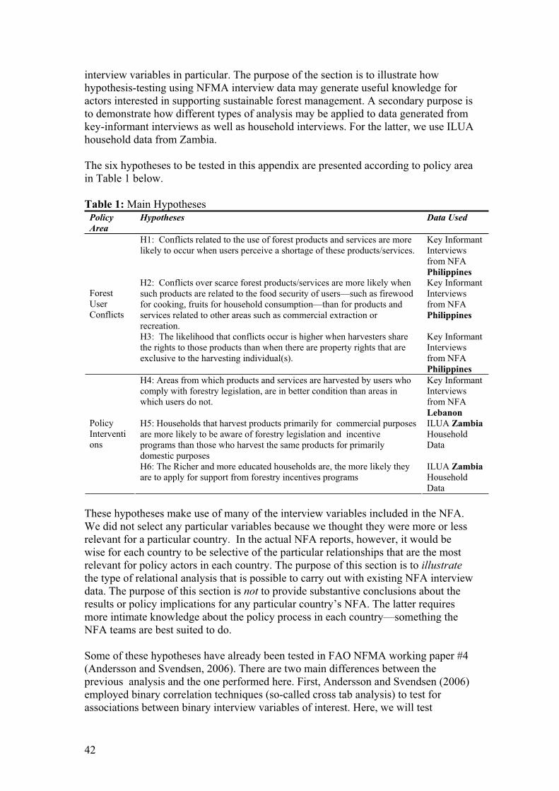
42

interview variables in particular. The purpose of the section is to illustrate how

hypothesis-testing using NFMA interview data may generate useful knowledge for

actors interested in supporting sustainable forest management. A secondary purpose is

to demonstrate how different types of analysis may be applied to data generated from

key-informant interviews as well as household interviews. For the latter, we use ILUA

household data from Zambia.

The six hypotheses to be tested in this appendix are presented according to policy area

in Table 1 below.

Table 1: Main HypothesesPolicy

Area

Hypotheses Data Used

H1: Conflicts related to the use of forest products and services are more

likely to occur when users perceive a shortage of these products/services.

Key Informant

Interviews

from NFA

Philippines

H2: Conflicts over scarce forest products/services are more likely when

such products are related to the food security of users—such as firewood

for cooking, fruits for household consumption—than for products and

services related to other areas such as commercial extraction or

recreation.

Key Informant

Interviews

from NFA

Philippines

Forest

User

Conflicts

H3: The likelihood that conflicts occur is higher when harvesters share

the rights to those products than when there are property rights that are

exclusive to the harvesting individual(s).

Key Informant

Interviews

from NFA

Philippines

H4: Areas from which products and services are harvested by users who

comply with forestry legislation, are in better condition than areas in

which users do not.

Key Informant

Interviews

from NFA

Lebanon

H5: Households that harvest products primarily for commercial purposes

are more likely to be aware of forestry legislation and incentive

programs than those who harvest the same products for primarily

domestic purposes

ILUA Zambia

Household

Data

Policy

Interventi

ons

H6: The Richer and more educated households are, the more likely they

are to apply for support from forestry incentives programs

ILUA Zambia

Household

Data

These hypotheses make use of many of the interview variables included in the NFA.

We did not select any particular variables because we thought they were more or less

relevant for a particular country. In the actual NFA reports, however, it would be

wise for each country to be selective of the particular relationships that are the most

relevant for policy actors in each country. The purpose of this section is to illustrate

the type of relational analysis that is possible to carry out with existing NFA interview

data. The purpose of this section is not to provide substantive conclusions about the

results or policy implications for any particular country’s NFA. The latter requires

more intimate knowledge about the policy process in each country—something the

NFA teams are best suited to do.

Some of these hypotheses have already been tested in FAO NFMA working paper #4

(Andersson and Svendsen, 2006). There are two main differences between the

previous analysis and the one performed here. First, Andersson and Svendsen (2006)

employed binary correlation techniques (so-called cross tab analysis) to test for

associations between binary interview variables of interest. Here, we will test

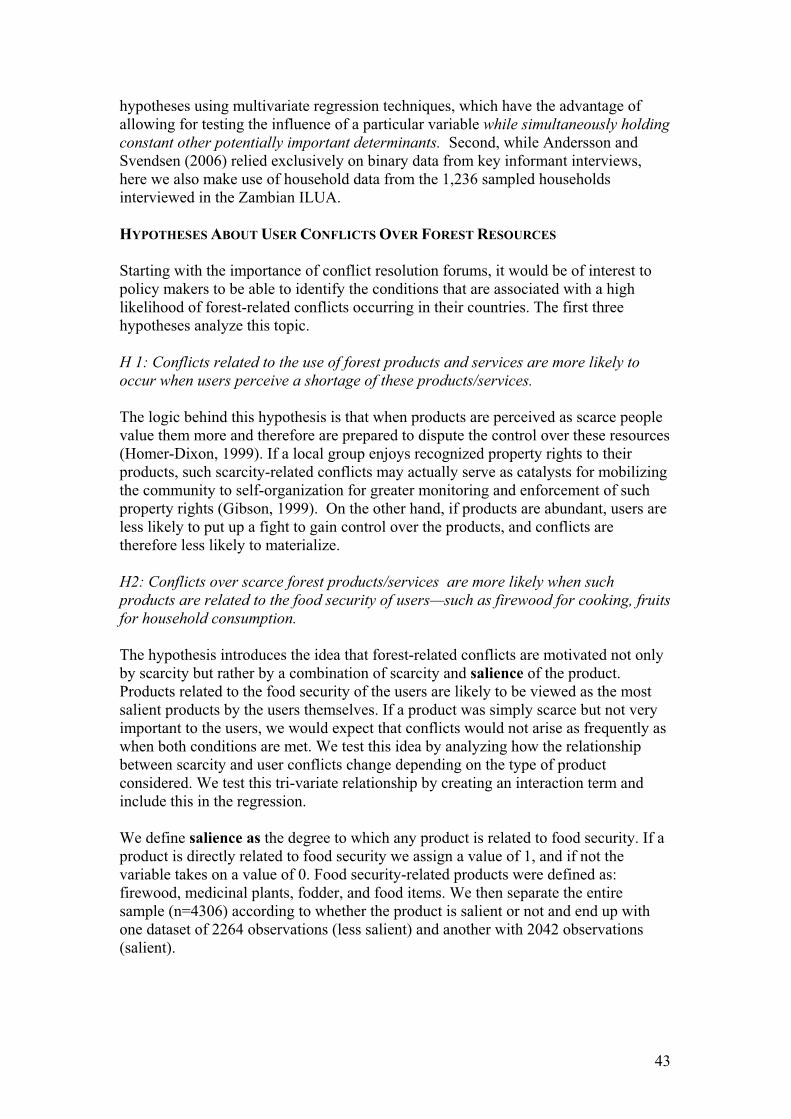
43

hypotheses using multivariate regression techniques, which have the advantage of

allowing for testing the influence of a particular variable while simultaneously holding

constant other potentially important determinants. Second, while Andersson and

Svendsen (2006) relied exclusively on binary data from key informant interviews,

here we also make use of household data from the 1,236 sampled households

interviewed in the Zambian ILUA.

HYPOTHESES ABOUT USER CONFLICTS OVER FOREST RESOURCES

Starting with the importance of conflict resolution forums, it would be of interest to

policy makers to be able to identify the conditions that are associated with a high

likelihood of forest-related conflicts occurring in their countries. The first three

hypotheses analyze this topic.

H 1: Conflicts related to the use of forest products and services are more likely to

occur when users perceive a shortage of these products/services.

The logic behind this hypothesis is that when products are perceived as scarce people

value them more and therefore are prepared to dispute the control over these resources

(Homer-Dixon, 1999). If a local group enjoys recognized property rights to their

products, such scarcity-related conflicts may actually serve as catalysts for mobilizing

the community to self-organization for greater monitoring and enforcement of such

property rights (Gibson, 1999). On the other hand, if products are abundant, users are

less likely to put up a fight to gain control over the products, and conflicts are

therefore less likely to materialize.

H2: Conflicts over scarce forest products/services are more likely when such

products are related to the food security of users—such as firewood for cooking, fruits

for household consumption.

The hypothesis introduces the idea that forest-related conflicts are motivated not only

by scarcity but rather by a combination of scarcity and salience of the product.

Products related to the food security of the users are likely to be viewed as the most

salient products by the users themselves. If a product was simply scarce but not very

important to the users, we would expect that conflicts would not arise as frequently as

when both conditions are met. We test this idea by analyzing how the relationship

between scarcity and user conflicts change depending on the type of product

considered. We test this tri-variate relationship by creating an interaction term and

include this in the regression.

We define salience as the degree to which any product is related to food security. If a

product is directly related to food security we assign a value of 1, and if not the

variable takes on a value of 0. Food security-related products were defined as:

firewood, medicinal plants, fodder, and food items. We then separate the entire

sample (n=4306) according to whether the product is salient or not and end up with

one dataset of 2264 observations (less salient) and another with 2042 observations

(salient).

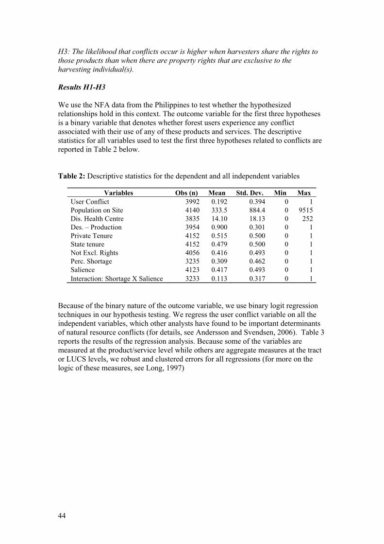
44

H3: The likelihood that conflicts occur is higher when harvesters share the rights to

those products than when there are property rights that are exclusive to the

harvesting individual(s).

Results H1-H3

We use the NFA data from the Philippines to test whether the hypothesized

relationships hold in this context. The outcome variable for the first three hypotheses

is a binary variable that denotes whether forest users experience any conflict

associated with their use of any of these products and services. The descriptive

statistics for all variables used to test the first three hypotheses related to conflicts are

reported in Table 2 below.

Table 2: Descriptive statistics for the dependent and all independent variables

Variables Obs (n) Mean Std. Dev. Min Max

User Conflict 3992 0.192 0.394 0 1

Population on Site 4140 333.5 884.4 0 9515

Dis. Health Centre 3835 14.10 18.13 0 252

Des. – Production 3954 0.900 0.301 0 1

Private Tenure 4152 0.515 0.500 0 1

State tenure 4152 0.479 0.500 0 1

Not Excl. Rights 4056 0.416 0.493 0 1

Perc. Shortage 3235 0.309 0.462 0 1

Salience 4123 0.417 0.493 0 1

Interaction: Shortage X Salience 3233 0.113 0.317 0 1

Because of the binary nature of the outcome variable, we use binary logit regression

techniques in our hypothesis testing. We regress the user conflict variable on all the

independent variables, which other analysts have found to be important determinants

of natural resource conflicts (for details, see Andersson and Svendsen, 2006). Table 3

reports the results of the regression analysis. Because some of the variables are

measured at the product/service level while others are aggregate measures at the tract

or LUCS levels, we robust and clustered errors for all regressions (for more on the

logic of these measures, see Long, 1997)

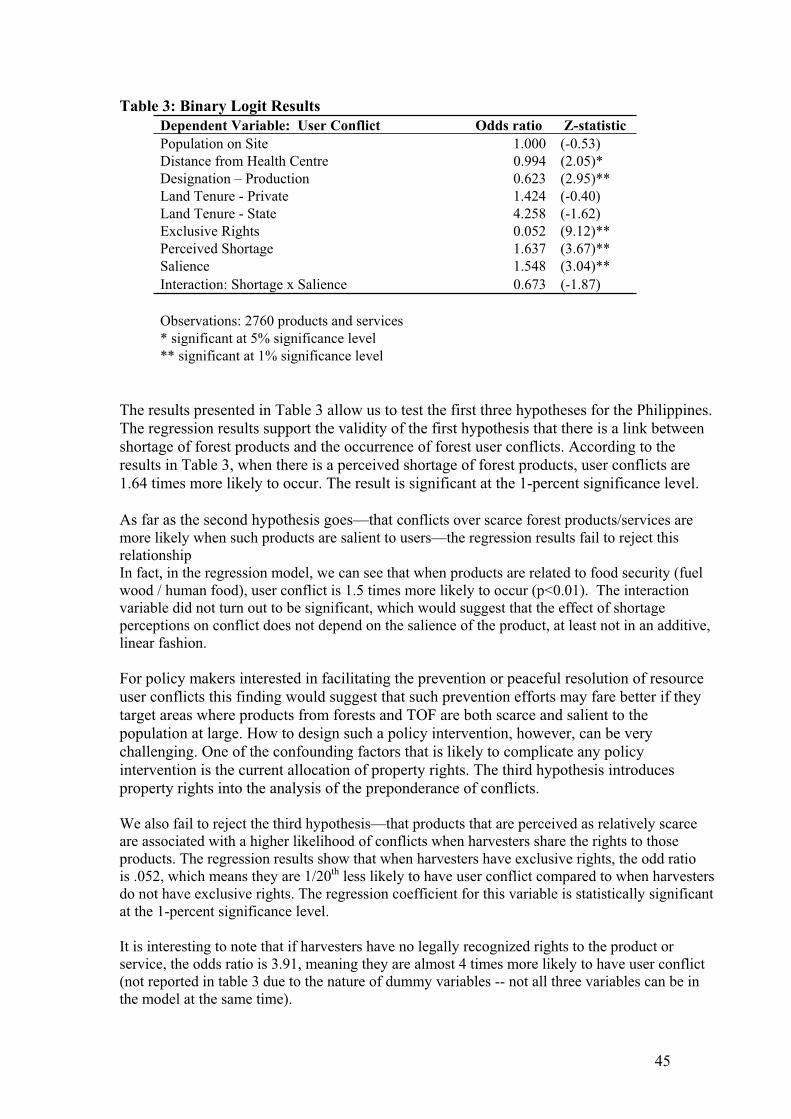
45

Table 3: Binary Logit Results

Dependent Variable: User Conflict Odds ratio Z-statistic

Population on Site 1.000 (-0.53)

Distance from Health Centre 0.994 (2.05)*

Designation – Production 0.623 (2.95)**

Land Tenure - Private 1.424 (-0.40)

Land Tenure - State 4.258 (-1.62)

Exclusive Rights 0.052 (9.12)**

Perceived Shortage 1.637 (3.67)**

Salience 1.548 (3.04)**

Interaction: Shortage x Salience 0.673 (-1.87)

Observations: 2760 products and services

* significant at 5% significance level

** significant at 1% significance level

The results presented in Table 3 allow us to test the first three hypotheses for the Philippines.

The regression results support the validity of the first hypothesis that there is a link between

shortage of forest products and the occurrence of forest user conflicts. According to the

results in Table 3, when there is a perceived shortage of forest products, user conflicts are

1.64 times more likely to occur. The result is significant at the 1-percent significance level.

As far as the second hypothesis goes—that conflicts over scarce forest products/services are

more likely when such products are salient to users—the regression results fail to reject this

relationship

In fact, in the regression model, we can see that when products are related to food security (fuel

wood / human food), user conflict is 1.5 times more likely to occur (p<0.01). The interaction

variable did not turn out to be significant, which would suggest that the effect of shortage

perceptions on conflict does not depend on the salience of the product, at least not in an additive,

linear fashion.

For policy makers interested in facilitating the prevention or peaceful resolution of resource

user conflicts this finding would suggest that such prevention efforts may fare better if they

target areas where products from forests and TOF are both scarce and salient to the

population at large. How to design such a policy intervention, however, can be very

challenging. One of the confounding factors that is likely to complicate any policy

intervention is the current allocation of property rights. The third hypothesis introduces

property rights into the analysis of the preponderance of conflicts.

We also fail to reject the third hypothesis—that products that are perceived as relatively scarce

are associated with a higher likelihood of conflicts when harvesters share the rights to those

products. The regression results show that when harvesters have exclusive rights, the odd ratio

is .052, which means they are 1/20th less likely to have user conflict compared to when harvesters

do not have exclusive rights. The regression coefficient for this variable is statistically significant

at the 1-percent significance level.

It is interesting to note that if harvesters have no legally recognized rights to the product or

service, the odds ratio is 3.91, meaning they are almost 4 times more likely to have user conflict

(not reported in table 3 due to the nature of dummy variables -- not all three variables can be in

the model at the same time).

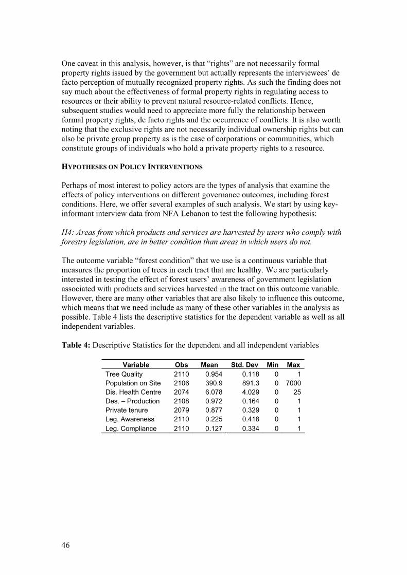
46

One caveat in this analysis, however, is that “rights” are not necessarily formal

property rights issued by the government but actually represents the interviewees’ de

facto perception of mutually recognized property rights. As such the finding does not

say much about the effectiveness of formal property rights in regulating access to

resources or their ability to prevent natural resource-related conflicts. Hence,

subsequent studies would need to appreciate more fully the relationship between

formal property rights, de facto rights and the occurrence of conflicts. It is also worth

noting that the exclusive rights are not necessarily individual ownership rights but can

also be private group property as is the case of corporations or communities, which

constitute groups of individuals who hold a private property rights to a resource.

HYPOTHESES ON POLICY INTERVENTIONS

Perhaps of most interest to policy actors are the types of analysis that examine the

effects of policy interventions on different governance outcomes, including forest

conditions. Here, we offer several examples of such analysis. We start by using key-

informant interview data from NFA Lebanon to test the following hypothesis:

H4: Areas from which products and services are harvested by users who comply with

forestry legislation, are in better condition than areas in which users do not.

The outcome variable “forest condition” that we use is a continuous variable that

measures the proportion of trees in each tract that are healthy. We are particularly

interested in testing the effect of forest users’ awareness of government legislation

associated with products and services harvested in the tract on this outcome variable.

However, there are many other variables that are also likely to influence this outcome,

which means that we need include as many of these other variables in the analysis as

possible. Table 4 lists the descriptive statistics for the dependent variable as well as all

independent variables.

Table 4: Descriptive Statistics for the dependent and all independent variables

Variable Obs Mean Std. Dev Min Max

Tree Quality 2110 0.954 0.118 0 1

Population on Site 2106 390.9 891.3 0 7000

Dis. Health Centre 2074 6.078 4.029 0 25

Des. – Production 2108 0.972 0.164 0 1

Private tenure 2079 0.877 0.329 0 1

Leg. Awareness 2110 0.225 0.418 0 1

Leg. Compliance 2110 0.127 0.334 0 1

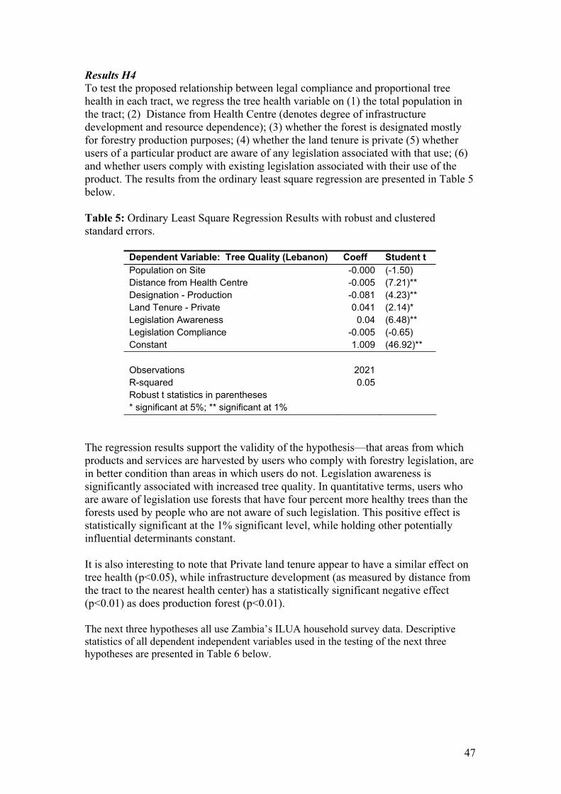
47

Results H4

To test the proposed relationship between legal compliance and proportional tree

health in each tract, we regress the tree health variable on (1) the total population in

the tract; (2) Distance from Health Centre (denotes degree of infrastructure

development and resource dependence); (3) whether the forest is designated mostly

for forestry production purposes; (4) whether the land tenure is private (5) whether

users of a particular product are aware of any legislation associated with that use; (6)

and whether users comply with existing legislation associated with their use of the

product. The results from the ordinary least square regression are presented in Table 5

below.

Table 5: Ordinary Least Square Regression Results with robust and clustered

standard errors.

Dependent Variable: Tree Quality (Lebanon) Coeff Student t

Population on Site -0.000 (-1.50)

Distance from Health Centre -0.005 (7.21)**

Designation - Production -0.081 (4.23)**

Land Tenure - Private 0.041 (2.14)*

Legislation Awareness 0.04 (6.48)**

Legislation Compliance -0.005 (-0.65)

Constant 1.009 (46.92)**

Observations 2021

R-squared 0.05

Robust t statistics in parentheses

* significant at 5%; ** significant at 1%

The regression results support the validity of the hypothesis—that areas from which

products and services are harvested by users who comply with forestry legislation, are

in better condition than areas in which users do not. Legislation awareness is

significantly associated with increased tree quality. In quantitative terms, users who

are aware of legislation use forests that have four percent more healthy trees than the

forests used by people who are not aware of such legislation. This positive effect is

statistically significant at the 1% significant level, while holding other potentially

influential determinants constant.

It is also interesting to note that Private land tenure appear to have a similar effect on

tree health (p<0.05), while infrastructure development (as measured by distance from

the tract to the nearest health center) has a statistically significant negative effect

(p<0.01) as does production forest (p<0.01).

The next three hypotheses all use Zambia’s ILUA household survey data. Descriptive

statistics of all dependent independent variables used in the testing of the next three

hypotheses are presented in Table 6 below.

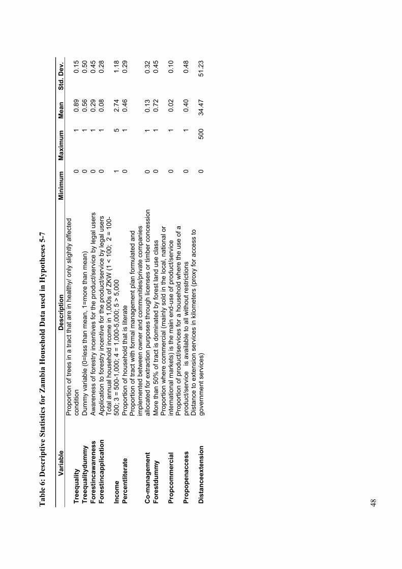
48

Ta

ble

6:

Des

crip

tiv

e S

tati

stic

s fo

r Z

am

bia

Ho

use

ho

ld D

ata

use

d i

n H

yp

oth

eses

5-7

Va

riab

le

De

sc

rip

tio

n

Min

imu

m

Ma

xim

um

M

ea

n

Std

. D

ev.

Tre

eq

uality

P

rop

ort

ion o

f tr

ees in

a tra

ct th

at are

in h

ealthy/ only

slig

htly a

ffe

cte

d

co

nditio

n

01

0.8

90.1

5

Tre

eq

uality

du

mm

y

Du

mm

y v

ari

ab

le (

0=

less t

han

mea

n,

1=

more

th

an

mea

n)

01

0.5

60.5

0

Fo

resti

ncaw

are

ness

A

wa

ren

ess o

f fo

restr

y incen

tive

s for

the p

roduct/se

rvic

e b

y le

ga

l u

sers

0

10

.29

0.4

5

Fo

resti

nca

pp

licati

on

A

pplic

ation to

fo

restr

y incentive fo

r th

e p

rodu

ct/

serv

ice b

y leg

al use

rs

01

0.0

80.2

8

Inco

me

Tota

l an

nual ho

usehold

incom

e in

1,0

00s o

f Z

KW

(1

< 1

00; 2

= 1

00

- 5

00

; 3

= 5

00

-1,0

00

; 4

= 1

,00

0-5

,00

0; 5

> 5

,00

0

15

2.7

41.1

8

Perc

en

tlit

era

te

Pro

port

ion o

f ho

usehold

that is

litera

te

01

0.4

60.2

9

Co

-ma

nag

em

en

t

Pro

port

ion o

f tr

act

with

fo

rma

l m

an

agem

ent p

lan

fo

rmu

late

d a

nd

im

ple

men

ted b

etw

een

ow

ne

r an

d c

om

mu

nitie

s/p

riva

te c

om

panie

s

allo

ca

ted f

or

extr

action

purp

ose

s t

hro

ugh

lic

en

ses o

r tim

be

r con

cessio

n0

10

.13

0.3

2

Fo

restd

um

my

M

ore

th

an

50%

of tr

act

is d

om

inate

d b

y fo

rest la

nd

use c

lass

01

0.7

20.4

5

Pro

pc

om

merc

ial

Pro

port

ion w

he

re c

om

merc

ial (m

ain

ly s

old

in the

lo

ca

l, n

ation

al or

inte

rnational m

ark

ets

) is

th

e m

ain

en

d-u

se o

f pro

du

ct/serv

ice

0

10

.02

0.1

0

Pro

po

pen

acc

es

s

Pro

port

ion o

f pro

duct/serv

ice

s for

a h

ouseh

old

wh

ere

th

e u

se

of a

p

rodu

ct/

serv

ice is a

va

ilable

to

all

witho

ut

restr

ictio

ns

01

0.4

00.4

8

Dis

tan

ceex

ten

sio

n

Dis

tance to e

xte

nsio

n s

erv

ices in k

ilom

ete

rs (

pro

xy for

acce

ss t

o

govern

ment serv

ices)

05

00

34

.47

51.2

3

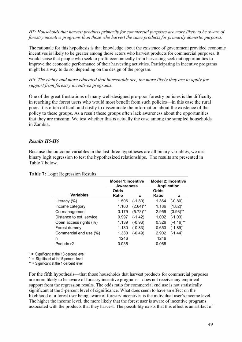
49

H5: Households that harvest products primarily for commercial purposes are more likely to be aware of

forestry incentive programs than those who harvest the same products for primarily domestic purposes.

The rationale for this hypothesis is that knowledge about the existence of government provided economic

incentives is likely to be greater among those actors who harvest products for commercial purposes. It

would sense that people who seek to profit economically from harvesting seek out opportunities to

improve the economic performance of their harvesting activities. Participating in incentive programs

might be a way to do so, depending on the design of the program.

H6: The richer and more educated that households are, the more likely they are to apply for

support from forestry incentives programs.

One of the great frustrations of many well-designed pro-poor forestry policies is the difficulty

in reaching the forest users who would most benefit from such policies—in this case the rural

poor. It is often difficult and costly to disseminate the information about the existence of the

policy to these groups. As a result these groups often lack awareness about the opportunities

that they are missing. We test whether this is actually the case among the sampled households

in Zambia.

Results H5-H6

Because the outcome variables in the last three hypotheses are all binary variables, we use

binary logit regression to test the hypothesized relationships. The results are presented in

Table 7 below.

Table 7: Logit Regression Results

Model 1:Incentive Awareness

Model 2: Incentive Application

VariablesOddsRatio z

OddsRatio z

Literacy (%) 1.506 (-1.80) 1.364 (-0.80)

Income category 1.160 (2.64)** 1.186 (1.82)'

Co-management 3.179 (5.73)** 2.959 (3.98)**

Distance to ext. service 0.997 (-1.42) 1.002 (-1.03)

Open access rights (%) 1.139 (-0.96) 0.326 (-4.16)**

Forest dummy 1.130 (-0.83) 0.653 (-1.89)'

Commercial end use (%) 1.330 (-0.49) 2.902 (-1.44)

n 1246 1246

Pseudo r2 0.035 0.068

‘ = Significant at the 10-percent level * = Significant at the 5-percent level ** = Significant at the 1-percent level

For the fifth hypothesis—that those households that harvest products for commercial purposes

are more likely to be aware of forestry incentive programs—does not receive any empirical

support from the regression results. The odds ratio for commercial end use is not statistically

significant at the 5-percent level of significance. What does seem to have an effect on the

likelihood of a forest user being aware of forestry incentives is the individual user’s income level.

The higher the income level, the more likely that the forest user is aware of incentive programs

associated with the products that they harvest. The possibility exists that this effect is an artifact of

50

the specific products that the country’s incentive programs target, and these products may not be

harvested by the poorest households. Another variable that has a significant and positive effect on

the likelihood of incentive awareness is the existence of co-management activities, in which

multiple actors have agreed to share management responsibilities to a forest that is held in

common. This variable has the strongest effect of all independent variables in the first model.

The regression results lend weak support to sixth hypothesis and the notion that richer and

more educated household members are more likely to apply to forestry incentives programs.

The odds ratios for the literacy and income variables are both greater then 1, meaning that the

effect is positive, but none of them are statistically significant at the 5-percent level. The

income variable is significant at the 10-percent level. Two other independent variables seem

to have the strongest effects on the likelihood of a household applying for forestry incentives.

Again co-management has a strong positive effect while the proportion of forest lands whose

access is not regulated and may therefore be considered open-access has a strong negative

effect. Households that harvest products primarily from open access forest lands are almost 60

percent less likely to apply for forestry incentive programs than users who harvest primarily

from forests that are not open access in nature.

CONCLUSION

In this brief appendix, we have tried to illustrate how the statistical analysis of interview data

may be used to learn about several relationships between variables that are relevant for public

policy in a variety of different contexts. We tested the strength and direction of the

relationships spelled out in the six hypotheses presented at the beginning of the appendix. We

found that using data from interviews enabled us to uncover several statistically significant

relationships between socioeconomic, institutional and biophysical variables. We believe this

is a good testament to the additional explanatory power that interview data bring to the

NFMA.

As NFMAs repeat data collection over time, the degree to which NFMA users will be able to

identify the factors that explain longitudinal changes in forests will depend to a great extent

on the availability of reliable and valid socioeconomic and institutional data collected through

interviews.

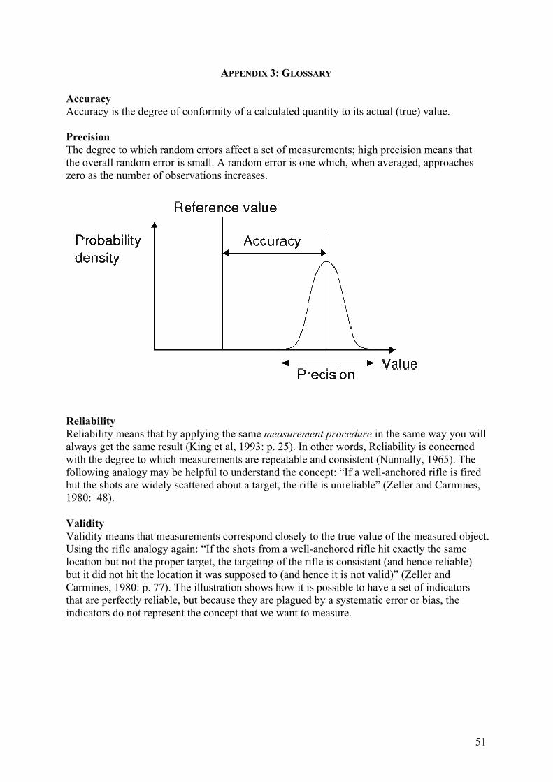
51

APPENDIX 3: GLOSSARY

Accuracy

Accuracy is the degree of conformity of a calculated quantity to its actual (true) value.

Precision

The degree to which random errors affect a set of measurements; high precision means that

the overall random error is small. A random error is one which, when averaged, approaches

zero as the number of observations increases.

Reliability

Reliability means that by applying the same measurement procedure in the same way you will

always get the same result (King et al, 1993: p. 25). In other words, Reliability is concerned

with the degree to which measurements are repeatable and consistent (Nunnally, 1965). The

following analogy may be helpful to understand the concept: “If a well-anchored rifle is fired

but the shots are widely scattered about a target, the rifle is unreliable” (Zeller and Carmines,

1980: 48).

Validity

Validity means that measurements correspond closely to the true value of the measured object.

Using the rifle analogy again: “If the shots from a well-anchored rifle hit exactly the same

location but not the proper target, the targeting of the rifle is consistent (and hence reliable)

but it did not hit the location it was supposed to (and hence it is not valid)” (Zeller and

Carmines, 1980: p. 77). The illustration shows how it is possible to have a set of indicators

that are perfectly reliable, but because they are plagued by a systematic error or bias, the

indicators do not represent the concept that we want to measure.

52

Reporting unit is an administrative or ecological region for which the NFI estimates are

calculated and reported. The entire area of a country can be divided into non-overlapping

reporting units. The union of the units comprises the entire area of the country. Note that this

means stratified sampling.

Design unit is a region in which the same NFI method is applied, including field data and

field plot density as well as remote sensing data. The union of the design units is the entire

area of the country.

APPENDIX 4: COMPARING ALTERNATIVE SAMPLING DESIGNS FOR NATIONAL AND

REGIONAL FOREST MONITORING

Comparing alternative sampling designs forNational and regional forest monitoring

Erkki Tomppo and Matti KatilaFinnish Forest Research Institute, National Forest Inventory

October 31, 2008

Abstract

We present a method to compare the efficiencies of the sampling de-signs of forest inventories by means of the standard errors of the se-lected parameters and field measurement costs. The method is appliedto the designs of United Nations FAO National Forest Monitoring andAssessment (NFMA)), the proposed ’Eurogrid’ designs of EuropeanUnion, as well as systematic or stratified cluster-wise sampling de-sign. Thematic maps of the Finnish multi-source forest inventory areemployed as models of forests in the simulation study. The mea-suring costs of different designs are assessed using information fromFinnish national forest inventory and earlier time studies. The walk-ing distances are assessed using GIS -based analysis on the maps ofmulti-source inventory. A similar technique without GIS -based costanalysis has been applied in designing Finnish National forest inven-tory in an operative way since early 1990’s.

The study shows that the FAO NFMA design, consisting of tractsof four field plots and Eurogrid consisting of detach observation points,is inefficient when comparing to cluster-wise design with samplingdensity adapted to variability of forests.

The presented method can be employed with any georeferenceddata, including information of the variables of interest and having aspatial resolution of about the size of the sampling unit and ,e.g., withremote sensing based land land cover or land use predictions or forestmanagement data.

KEYWORDS: forest inventory, sampling simulation, standard error, GIS

1 Introduction

The Food and Agriculture Organization of the United Nations (FAO) has collected

global level forest information since 1947. UN-ECE/FAO (United Nations Eco-

nomic Commission for Europe/FAO) has co-operated with FAO in collecting and

publishing the Temperate and Boreal region data (UN-ECE/FAO, 2000). The lat-

est report, FRA 2005 was published in late 2005. Forest resources assessment is

mainly based on NFI systems at national and regional levels. These schemes were

set up to fulfill national needs and international commitments, such as the Forest

Resource Assessment (FRA) conducted by FAO every 10th year, or currently ev-

ery 5th year. Although countries report to these global resources assessments, the

base definitions in the countries are not harmonized. The process of converting

national NFI data to international UN/FAO requests is done individually by each

country without any mechanism to control the comparability and the harmoniza-

tion of these reports. That is, in spite of global definitions, there are no specific

harmonization tools and processes to fulfill EU needs such as market oriented

production or environmental EU requirements (MCPFE indicators for example).

Countries are planning and conducting the inventories on the basis of their

own information needs and traditions. Some countries have long traditions, from

the beginning of 1920s, while other countries have conducted just one inventory or

are even planning the first sampling based inventory, or at a global level, are lack-

ing even the first inventory. While some inventories are wood production oriented,

some other inventories are targeted to produce information about non-wood goods

and services, or are multi-purpose inventories. Most inventories collect informa-

tion on the same base variables; however, some inventories collect some hundreds

of parameters measured on the field. Most of the current NFIs are sampling-based

inventories. Countries that were conducting stand level inventories are moving

slowly to sampling-based inventories, using in many cases, remotely sensed data

as ancillary information.

FAO has carried out excellent work in assisting countries in establishing their

forest inventories. In addition to the common definitions and support work, e.g.,

through regional meetings and training schools, targeted to Forest resource As-

sessment (FRA) program, a comprehensive inventory method called National For-

est Monitoring and Assessment (NFMA) has been established (FAO, 2008). Cur-

rently, NFA has been completed in seven countries (Bangladesh, Cameroon, Costa

Rica, Guatemala, Honduras, Lebanon and Phillipines), is in progress in ten coun-

tries (Angola, Republic of Congo, Kenya, Kyrgyzstan, Zambia, Brazil, Algeria,

Nicaragua, Uruguay and Comoros) and Formulated for eight countries (Cuba,

56

Nigeria, Vietnam, Tanzania, Ecuador, Uzbekistan, The Gambia and Macedonia,

FAO 2008).

European administrations and policy makers need comprehensive data on for-

est resources at the European level. Information on forest resources has tradi-

tionally been used for forest policy decision making by Member States, taken at

the national and sub-national levels. Practically all of the Member States collect

forest data through national forest inventories (NFIs). NFIs provide information

relevant for national level decision making, policy formulation and monitoring

for forestry and relevant sectors, as well as for forestry planning in smaller geo-

graphical or political units at the sub-national level. During the past decades, the

scope of forestry has become wider and the information needs have increased. The

monitoring of forest resources for assessing the vitality of trees and forests, forest

biodiversity and the role of forests in global carbon cycle have become important

issues. NFIs already provide information on some or all of these topics.

In addition to forest inventories at the national level, other monitoring efforts

were established in Europe by the European Commission. In particular, two reg-

ulations on the monitoring of the effect of atmospheric pollution and forest fires

were established in 1987 and 1992, respectively. hese were the Reg. 3528/86 on

the Monitoring of Atmospheric Pollution in Forests and Reg. 2158/92 on Forest

Fire Prevention. This latter regulation was complemented by Reg. 804/94 for

the establishment of an information system for forest fires, the so-called Common

Core Forest Fires Database.

A topical question in Europe is should European forest information supply be

established on harmonized and strengthened NFIS or should some kind of Euro-

pean level forest inventory system be established. An advantage of NFIs is that

the sampling designs and information content have been adapted to national and

local variability of forests and information needs. A drawback is the lack of har-

monization.

European Union COST Action E43 was launched to harmonize definitions and

concepts of European NFIs in such a way that NFIs could provide comparable

data (www.metla.fi/eu/cost/e43/). On the other hand, a unified Eurogrid has been

proposed. The grid would consist of detached points, with distances, e.g., of 16

km × 16 km or 4 km × 4 km.

Let us first recall some basic concepts of in sampling theory.

1. Target population is a set of the elements for which the inference is to be

made. Population can be discrete (finite or infinite) or continuous (always infinite,

e.g. a real plane, a forest area).

2. A sample s is a subset of the population.

57

3. Sampling frame is the mechanism which allows to identify the elements in

the population.

4. The set of all samples is denoted by S.

5. Selection probability of a sample is denoted by p(s). The sampling frame

usually determines the selection probability of each sample.

6. Inclusion probability of an element,

πi = ∑s:Ui∈s

p(s) 1

tells the probability that an individual Ui is included in an arbitrary sample. Note

that the inclusion probabilities can vary and that the most efficient sampling pro-

cedures often rest upon unequal probabilities (e.g., Mandallaz 2008, see also Gre-

goire and Valentine 2008).

One basic principle in probability sampling is that each element in the popula-

tion must have a positive inclusion probability. The inference concerns that set of

the elements which have a positive inclusion probability. Note that each sample s

does not have to have a positive inclusion probability. It is important to take into

account the unequal probabilities in the inference. Otherwise, biased estimates

may result.

In this study, the efficiencies of NFMA design and the proposed Eurogrid

design (denoted by EUROGRID) of detached plots of 4 km × 4 km grid are com-

pared to cluster-wise designs. The two basic plot densities are 1) the density

corresponding the NFMA design one tract at the crossing of every latitude and

longitude, and 2) the plot density with a plot grid 4 km x 4 km. The samples

are picked up from the output thematic maps of the Finnish multi-source National

Forest Inventory. A similar method has been used in NFI designing since early

1990s (Tomppo et al. 2001, Katila and Tomppo 2006). The costs are based on

costs studies in planning the design of the Finnish NFI (Päivinen and Yli-Kojola

1983, Henttonen 1991). Furthermore, walking time in forests is assessed using

data base of Land Survey Finland and GIS analysis. The purpose is not to present

an optimal design with some given costs, but rather to demonstrate a method that

could be applied in sampling studies at global and European level, and particu-

larly that cluster-wise sampling design, possibly with some stratification, is more

efficient than a design consisting of nearby large plots or detached plots.

58

2 Study area and material

The study is conducted throughout Finland, the land area being 30.447 million

hectares and forestry land area 26.277 million hectares. The output maps from the

operative multi-source NFI are applied (Figure 1). The maps have been created

using field sample plots of the 9th NFI, in total about 70 000 plots on forestry

land in the country, satellite images, digital map data and non-parametric k-NN

estimation (e.g., Tomppo 1996, Katila and Tomppo, 2001, Tomppo and Halme,

2004, Tomppo et al. 2006, Tomppo et al. 2008a). The total volume of growing

stock on the basis of the NFI9 (1996-2003) is 2091 million m3, the volume of

Scots pine (Pinus sylvestris L.), 999.7 million m3 Norway spruce (Picea abies

(L.) Karst.), 694.7 million m3, birch (Betula spp.), 325.2 million m3 and other tree

species, mainly aspen (Populus tremula L.) and alder (Alnus spp.) 71.7 million m3.

The volume of saw timber is 626.9 million m3.

The applied output thematic maps of multi-source NFI employed in this study

are mean volume of growing stock of all tree species (denoted by ALL) (m3/ha),

mean volume of broad-leaved tree species other than birch (m3/ha) (denoted by

OBL) and the volume of saw timber (m3/ha) (denoted by SAW). All volumes

concern forestry land (FRYL). Note that forestry land is the union of forest land,

poorly productive forest land and unproductive forest land (Tomppo 2006a).

The volume of OBL represents a rare object in sampling inventory and the vol-

ume of saw timber stands for the trees with a DBH of at least 20 cm, employed in

NFMA. All themes include information about land use classes (Figure 1), making

it possible to estimate the error of forestry land area estimate.

3 Methods

3.1 Sampling simulation and designs

FAO NFMA design consists of tracts with four plots (FAO 2004). In the basic

design, the plots are located at the intersection of every latitude/longitude (FAO

2004). The trees with a DBH at least of 10 cm and less than 20 cm are measured

from the subplot 1 (SPL1) and the trees with a DBH at least 20 cm the whole plot.

Only the total number of trees by species is measured for tree with a DBH less

than 10 cm (SPL2).

We study the sampling errors of the following parameters:

a) area of forestry land (ha),

b) mean tree stem volume of growing stock (m3/ha),

59

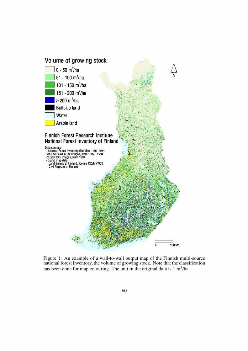
Figure 1: An example of a wall-to-wall output map of the Finnish multi-sourcenational forest inventory, the volume of growing stock. Note that the classification

has been done for map colouring. The unit in the original data is 1 m3/ha.

60

c) total tree stem volume of growing stock (m3),

d) mean volume of saw timber (m3/ha),

e) total volume of saw timber (m3),

f) mean tree stem volume of OBL (m3/ha) and

g) total tree stem volume of OBL (m3).

The estimates of parameter values on the multi-source inventory output maps

are: forestry land 26.42045 million hectares, total volume of all species 2059.1

million m3, mean volume of growing stock on forestry land of all species 77.9 m3/ha

with a standard deviation of volumes among pixels 68.3 m3/ha, the total volume

and mean volume of OBL species on forestry land 62.44 million m3 and 2.4 m3/ha

respectively, and the total and mean volume saw timber 613.8 million m3 and

23.23 m3/ha respectively.

The simulation was done for all designs as follows. The starting point was

selected randomly within a square corresponding to the distances in south-north

and west-east directions of two adjacent clusters or the distance of two adjacent

sample plots in Eurogrid. For all designs, 1000 samples were selected. The es-

timate of the parameter of interest, e.g., total volume, were computed from each

sample. The mean of the estimates of the parameter values as well the standard

deviation over samples were also computed,

sd =

√

∑nj=1(yi − y)2

n−12

where yi is the estimate of the parameter in ith simulation and y the average of

the estimates over the simulations.

On the basis of sampling error definition, the standard deviation (2) can be

used as sampling error.

The goal was to find two groups of sampling designs, a dense design group and

a sparse design group, in such a way that the errors of the estimates by parameters

and by groups were of about the same magnitude. This was achieved through

several sampling simulations using a method of trial and error. The starting design

for the dense design was a grid of detached plots with the distances of 4 km×4 km

(Eurogrid), and for the sparse design, the NFMA design with a NFMA type cluster

on every crossing of latitude and longitude.

The two groups which fulfill the given criteria, dense and sparse, and the final

designs for which the costs were calculated were as follows:

61

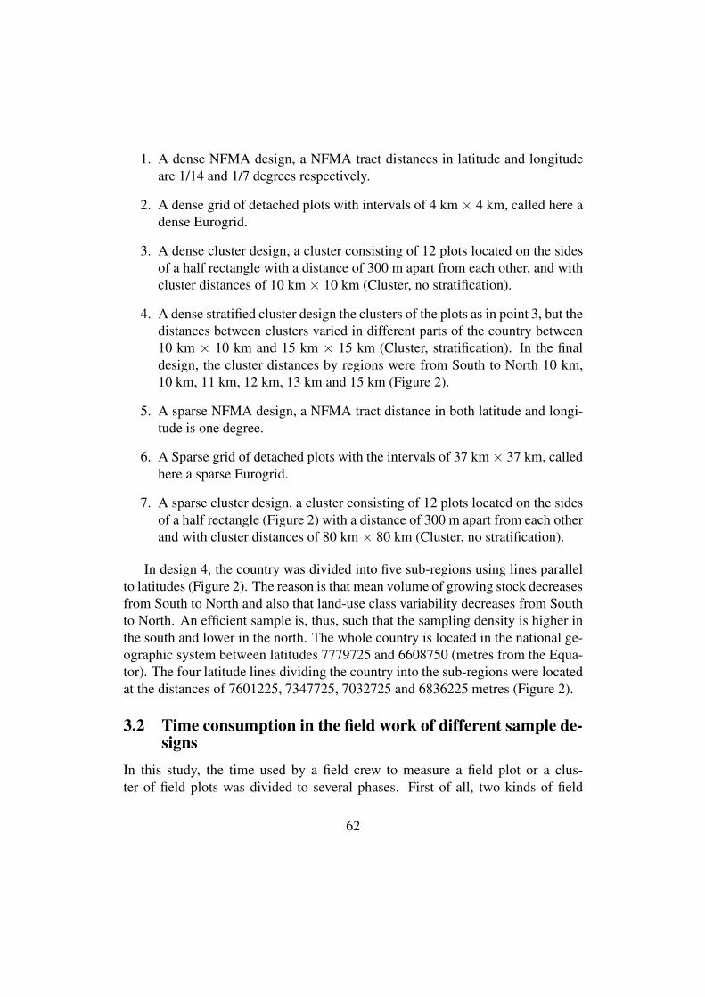
1. A dense NFMA design, a NFMA tract distances in latitude and longitude

are 1/14 and 1/7 degrees respectively.

2. A dense grid of detached plots with intervals of 4 km × 4 km, called here a

dense Eurogrid.

3. A dense cluster design, a cluster consisting of 12 plots located on the sides

of a half rectangle with a distance of 300 m apart from each other, and with

cluster distances of 10 km × 10 km (Cluster, no stratification).

4. A dense stratified cluster design the clusters of the plots as in point 3, but the

distances between clusters varied in different parts of the country between

10 km × 10 km and 15 km × 15 km (Cluster, stratification). In the final

design, the cluster distances by regions were from South to North 10 km,

10 km, 11 km, 12 km, 13 km and 15 km (Figure 2).

5. A sparse NFMA design, a NFMA tract distance in both latitude and longi-

tude is one degree.

6. A Sparse grid of detached plots with the intervals of 37 km × 37 km, called

here a sparse Eurogrid.

7. A sparse cluster design, a cluster consisting of 12 plots located on the sides

of a half rectangle (Figure 2) with a distance of 300 m apart from each other

and with cluster distances of 80 km × 80 km (Cluster, no stratification).

In design 4, the country was divided into five sub-regions using lines parallel

to latitudes (Figure 2). The reason is that mean volume of growing stock decreases

from South to North and also that land-use class variability decreases from South

to North. An efficient sample is, thus, such that the sampling density is higher in

the south and lower in the north. The whole country is located in the national ge-

ographic system between latitudes 7779725 and 6608750 (metres from the Equa-

tor). The four latitude lines dividing the country into the sub-regions were located

at the distances of 7601225, 7347725, 7032725 and 6836225 metres (Figure 2).

3.2 Time consumption in the field work of different sample de-signs

In this study, the time used by a field crew to measure a field plot or a clus-

ter of field plots was divided to several phases. First of all, two kinds of field

62

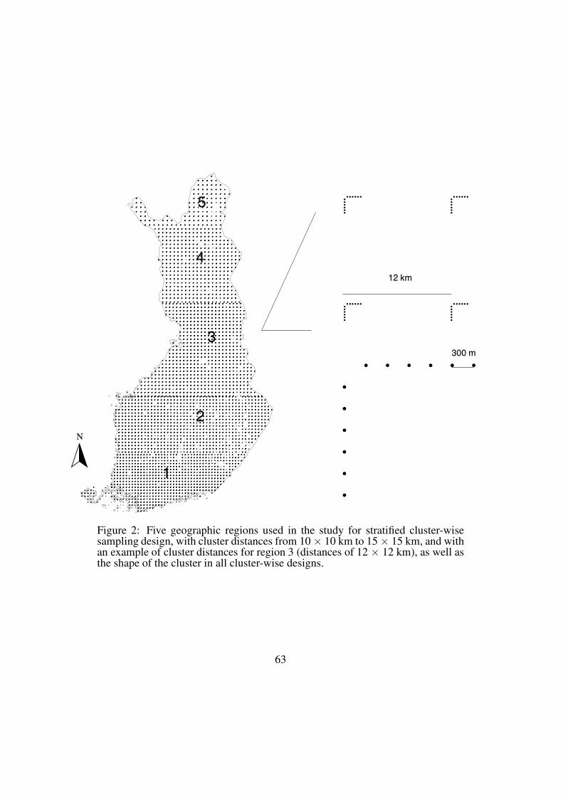
rrrrrrrr rrrrrrrrrrrr

rrrrrrrrrrr rrrrrrrrrrr

rrrrrrrrrrrr

rrrrrrrrrrrr

rrrrrrrrrrrr

rrrrrrrrrrrr

rrrrrrrrrrr

rrrrrrrrrrrr

rrrrrrrrrrrr

rrrrrrrrrrrr

rrrrrrrrrrr rrrrrrrrrrrr

rrrrrrrrrrrr

rrrrrrrrrrrr rrrrrrrrrrrr rrrrrrrrrrrr rrrrrrrrrrrr rrrrrrrrrrrr

rrrrrrrrrrrr

rrrrrrrrrrrr

rrrrrrrrrrrr

rrrrrrrrrrrr

rrrrrrrrrrrr

rrrrrrrrrrrr

rrrrrrrrrrrr

rrrrrrrrrrrr

rrrrrrrrrrrr

rrrrrrrrrrrr

rrrrrrrrrrrr

rrrrrrrrrrrr

rrrrrrrrrrrr

rrrrrrrrrrrr

rrrrrrrrrrrr

rrrrrrrrrrrr

rrrrrrrrrrrr

rrrrrrrrrrr

rrrrrrrrrrrr

rrrrrrrrrr

rrrrrrrrrrrr

rrrrrrr

rrrrrrrrrrrr

rrrrrrrrrrrr

rrrrrrrrrrr

rrrrrrrrrrrr

rrrrrrrrrrrr

rrrrrrrrrrrr

rrrrrrrrrrrr

rrrrrrrrrrrr

rrrrrrrrrrrr

rrrrrrr

rrrrrrrrrrrr

rrrrrrrr

rrrrrrrrrrrr

rrrrrrrrrrrr

rrrrrrrrrrrr

rrrrrrrrrrrr

rrrrrrrrrrrr

rrrrrrrrrrrr

rrrrrrrrrrrr

rrrrrrr

rrrrrrrrrrrr

rrrrrrrrrrr

rrrrrrrrrr

rrrrrrrrrrrr

rrrrrrrr

rrrrrrrrrrrr

rrrrrrrrrrrr

rrrrrrrrrrrr

rrrrrrrrrrrr

rrrrrrrrr

rrrrrrrrrrr

rrrrrrrrrrrr

rr

rrr

rrrrrrrrrrrr

rrrrrrrrrrrr

rrrrrrrrrrrr

rrrrrrrrrr

rrrrrrrrrrr

rrr

rr

rrrrrr

rrrrrrrrrrrr

rrrrrrrrrrrr

rrrrrrrrrrr

rrrrrrrrrrr

rrrrrrrrrr

rrrrrrrrrrrr

rrrrrrrrrrrr

rrrrrrrrrrr

rrrrrrrrr

rrrrrrrrrr

rrrrrrrrrrrr

rrrrrr

rrrrrrrr

rrrrrrrrrr

rrrrrrr

rrrrrr

rrrrrrrrrrr

rrrrrrrrrrrr rrrrrrrrrrr

rrrrrrrrrrr

rrrrrrrrrrrr

r

rrrrrrrrrrrr

rrrrrrrrrrrr

rrrrrrrrrrrr

rrrrrrrrrrr

rrrrrrrrrrrr

rrrrrrrrrrr

rrrrrrr

rrrrrrrrrrrr

rrrrrrrrrrrr

rrrrrrrrrrrr

rrrrrrrrrrr

rrrrrrrrrr

rrrrrrrrrrrr

rrrrrrrrrrrr

rrrrrr

rrrrrrrrrrrr

rrrrrrrrrrrr

rrrrrrrrrrrr

rrrrrrrrrrrr

rrrrrrrrrrr

rrrrrrrrrrrr

rrrrrrrrrrrr

rrrrrrrrrrrr

rrrrrrrrrrr

rrrrrrrrrrrr

rrrrrrrrrrrr

rrrrrrrrrrrr

rrrrrrrrrrrr

rrrrrrrrrrrr

rrrrrrrrrrr

rrrrrrrrrrrr

rrrrrrrrrrr

rrrrrrrrrrrr

rrrrrrrrrrrr

rrrrrrrrrrrr

rrrrrrrrrrrr

rrrrrrrrrrrr

rrrrrrrrrrrr

rrrrrrrrrrrr

rrrrrrrrrrrr

rrrrrrrrrrrr

rrrrrrrrrrrr

rrrrrrrrr

rrrrrrrrrrrr

rrrrrrrrrrrr

rrrrrrrrrrrr

rrrrrrrrrrr

rrrrrrrrrrrr

rrrrrrrrrrrr

rrrrrrrrrrrr

rrrrrrrrrrrr

rrrrrrrrrrrr

rrrrrrrrr

rrrrrrrrrrrr

rrrrrrrrrrr

rrrrrrrrrrrr

rrrrrrrrrrrr

rrrrrrrrrrrr

rrrrrrrrrrrr

rrrrrrrrrrr

rrrrrrrrrrrr

rrrrrrrrrrrr

rrrrrrrrrrr

rrrrrrrrrrrr

rrrrrrrrrrrr

rrrrrrrrrrrr

rrrrrrrrrrrr

rrrrrrrrrrrr

rrrrrrrrrrrr

rrrrrrrrrrrr

rrrrrrrrrrrr

rrrrrrrrrrrr

rrrrrrrrrrrr

rrrrr

rrrrrrrrrrrr

rrrrrrrrrrrr

rrrrrrrrrrrr

rrrrrrrrrrrr

rrrrrrrrrrrr

rrrrrrrrrrrr

rrrrrrrrrrrr

rrrrrrrrrrrr

rrrrrrrrrrrr

rrrrrrrrrrr

rrrrrrrrrrr

rrrrrrrrrrrr

rrrrrrrrrrrr

rrrrrrrrrrrr

rrrrrrrrrrrr

rrrrrrrrrrr

rrrrrrrrrrrr

rrrrrrrrrrrr

rrrrrrrrrrrr

rrrrrrrrrr

rrrrrrrrrrrr

rrrrrrrrrrrr

rrrrrrrrrrrr

rrrrrrrrrrrr

rrrrrrrrrrrr

rrrrrrrrrrrr

rrrrrrrrrrrr

rrrrrrrrrrrr

rrrrrrrrrrrr

rrrrrrrrrrr

rrrrrrrrrrr

rrrrrrrrrrrr

rrrrrrrrrrrr

rrrrrrrrrrrr

rrrr

rrrrrrrrrrrr

rrrrrrrrrrrr

rrrrrrrrrrrr

rrrrrrrrrrrr

rrrrrrrrrr

rrrrrrrrrrrr

rrrrrrrrrrrr

rrrrrrrrrrr

rrrrrr

rrrrrrrrrrrr

rrrrrrrrrrrr

rrrrrrrrrrr

rrrrrrrrrrrr

rrrrrrrrrrrr

rrrrrrrrrrrr

rrrrrrrrrrrr

rrrrrrrrrrrr

r

rrrrrrrrrrrr

rrrrrrrrrrr

rrrrrrrrrrr

rrrrrrrrrrrr

rrrrrrrrrrrr

rrrrrrrrrrrr

rrrrrrrrrr

rrrrrrrrr

rrrrrrrrrr

rrrrrrrrrrrr

rrrrrrrrrrrr

rrrrrrrrrrrr

rrrrrrrrrrrr

rrrrrrrrrrrr

rrrrrrrrrrrr

rrrrrrrrrrrr

rrrrrrrrrrrr

rrrrrrrrrrrr

rrrrrrrrrrrr

rrrrrrrrrrrr

rrrrrrrrrrrr

rrrrrrrrrr

rrrrrrrrrrr

rrrrrrrrrrrr

rrrrrrrrrrrr

rrrrrrrrrrrr

rrrrrrrrrrrr

rrrrrrrrr

rrrrrrrrrrrr

rrrrrrrrrrrr

rrrrrrrrrrrr

rrrrrrrrrrrr

rrrrrrrrrrrr

rrrrrrrrrrr

rrrrrrrrrrr

rrrrrrrrrrrr

rrrrrrrrrrrr

rrrrrrrrrrrr

rrrrrrrrrrrr

rrrrrrrrrrrr

rrrrrrr

rrrrrrrrrrrr

rrrrrrrrrrr

rrrrrrrrrrrr

rrrrrrrrrrrr

rrrrrrrrrrrr

rrrrrrrrrrrr

rrrrrrrrrrrr

rrrrrrrrrrrr

rrrrrrrrrrrr

rrrrrrrrrrr

rrrrrrrrrrrr

rrrrrrrrrrrr

rrrrrrrrrrrr

r

rrrrrrrrrrrr

rrrrrrrrrrrr

rrrrrrrrrrrr

rrrrrrrrr

rrrrrrrrrrrr

rrrrrrrrrrrr

rrrrrrrrrrrr

rrrrrrrrrrrr

rrrrrrrrrrrr

rrrrrrrrrrr

rrrrrrrrr

rrrrrrrrrrr

rrrrrrrrrr

rrrrrrrrrrrr

rrrrrrrrrrrr

rrrrrrrrrrrr

rrrrrrrrrrrr

rrrrrrrrrrrr

rrrrrrrrrrrr

rrrrrrrrrrrr

rrrrrrrrrrrr

rrrr

rrrrrrrrrrrr

rrrrrrrrrrrr

rrrrrrrrrrrr

rrrrrrrrrrrr

rrrrrrrrrrr

rrrrrrrrrrrr

rrrrrrrrrrr

rrrrrrrr

rrrrrrrrrrr

rrrr

rrrrrrrr

rrrrrrrrrrr

rrrrrrrrrrrr

rrrrrrrrrrrr

rrrrrrrrrrrr

rrrrrrrrrrrr

rrrrrrrrrrrr

rrrrrrrrrrrr

rrrrrrrrrrrr

rrrrrrrrrrrr

rrrrrrrrrrr

rrrrrrrrrrrr

rrrrrrrrrrrr

rrrrrrrrrrrr

rrrrrrrrrrr

rrrrrrrrrrrr

rrrrrrrrrrrr

rrrrrrrrrrr

rrrrrrrrrrrr

rrrrrrrrrrrr

rrrrrrrrrrr

rrrrrrrrrrrr

rrrrrrrrrrrr

rrrrrrrrrrrr

rrrrrrrrrrrr

rrrrrrrrrrrr

rrrrrrrrrrrr

rr

rrrrrrrrr

rrrrrrrrrrr

rrrrrrrrrrrr

rrrrrrrrrrrr

rrrrrr

rrrrrrrrrrrr

rrrrrrrrrrrr

rrrrrrrrrrrr

rrrrrrrrrrr

rrrrrrrrrrrr

rrrrrrrrrr

r

rrrrrrrrrr

rrrrrrrrrrrr

rrrrrrrrrrrr

rrrrrrrrrrr

rrrrrrrrrrrr

rrrrrrrrrrrr

rrrrrrrrrrrr

rrrrrrrrr

rr

rrrrrrrrrrrr

rrrrrrrrrrrr

rrrrrrrrrrrr

rrrrrrrrrrr

rrrrrrrrrrrr

rrrrrrrrrrrr

rrrrrrrrrrr

rrrrrrrrrrrr

rrrrrrrrrrrr

rrrrrrrrrr

rrrr

rrrrrrrrrrr

rrrrrrrrrr

rrrrrrrrrrrr

rrrrrrrrrrrr

rrrrrrrrrrrr

rrrrrrrr

rrrrrrrrrrrr

rrrrrr

rrrrrrrrrrrr

rrrrrrrrrrrr

rrrrrrrrrrrr

rrrrrrrrrrrr

rrrrrrrrrrrr

rrrrrrrrrrrr

rrrrrrrrrrrr

rrrrrrrrrrrr

rrrrrrrrrrrr

rrrrrrrrrrrr

rrrrrrrrrrrr

rrrrrrrrrr

rrrrrrrrrrrr

rrrrrrrrr

rrrrrrr

rrrrrrrrrrrr

rrrrrrrrrrr

rrrrrrrrrrrr

rrrrrrrrrrrr

rrrrrrrrrrrr

rrrrrrrrrrr

rrrrrrrrrrrr

rrrrrrrrrrrr

rrrrrrrrrrrr

rrrrrrrrrrrr

rrrrrrrrrrrr

rrrrrrrrrrrr

rrrrrrrrrrrr

rrrrrrrrrrrr

rrrrrrrrrrrr

rrrrrrrrrrrr

rrrrrrrrrrrr

rrrrrr

rrrrr

rrrrrrrrrrrr

rrrrrrrrrrrr

rrrrrrrrrrrr

rrrrrrrrrrrr

rrrrrrrrrrrr

rrrrrrrrrrrr

rrrrrrrrrrrr

rrrrrrrrrrrr

rrrrrrrrrrrr

rrrrrrrrrrrr

rrrrrrrrrrrr

rrrrrrrrrrrr

rrrrrrrrrrrr

rrrrrrrrrrrr

rrrrrrrrrrrr

rrrrrrrrrrrr

rrrrrrrrrrrr

rrrrrrrrrrrr

rrrrrrrrrrrr

rrrrrrrrrrrr

rrrrrrrrrrrr

rrrrrrrrrrrr

rrrrrrrrrrrr

rrrrrrrrrrrr

rrrrrrrrrrrr

rrrrrrrrrrrr

rrrrrrrrrrrr

rrrrrrrrrrrr

rrrrrrrrrrrr

rrrrrrrrrrrr

rrrrrrrrrrrr

rrrrrrrrrrrr

rrrrrrrrrrrr

rr

rrrrrrrrrrrr

rrrrrrrrrrrr

rrrrrrrrrrrr

rrrrrrrrrrrr

rrrrrrrrrrrr

rrrrrrrrrrrr

rrrrrrrrrrrr

rrrrrrrrrrrr

rrrrrrrrrrrr

rrrrrrrrrrrr

rrrrrrrrrrr

rrrrrrrrrr

rrrrrrrrrrrr

rrrrrrrrrrr

rrrrrrrrrrrr

rrrrrrrrrrrr

rrrrrrrrrrrr

rrrrrrrrrrrr

rrrrrrrr

rrrrrr

rrrrrrrrrrrr

rrrrrrrrrrrr

rrrrrrrrrrr

rrrrrr

rrrrrrrrrrrr

rrrrrrrrrrrr

rrrrrrrrrrrr

r

rrrrrr rr

rrr

rrr rrrrrrr

rrrrrrrrrr

rrrr

rrrrrrrrrrr

rrrrrrrrrrrr

rrrrrrrrrrrr

rrrrrrrrrrr

rrrrrrrrrrrr

rrrrrrrrrrrr

rrrrrrrrrrrr

rrrrrrrrrrrr

rrrrr

rrrrrrrrrr

rrrrrrrrrrrr

rrrrrrrrrrrr

rrrrrrrrrrrr

rrrrrrrrrrrr

rrrrrrrrrrrr

rrrrrrrrrrrr

rrrrrrrrrrrr

rrrrrrrrrrrr

rrrrrrrrrrrr

rrrrrrrrrrrr

rrrrrrrrrrrr

rrrrrrrrrrrr

rrrrrrrrrrrr

rrrrrrrrrrrr

rrrrrrrrrrrr

rrrrrrrrrrrr

rrrrrrrrrrrr

rrrrrrrrrrrr

rrrrrrrrrrrr

rrrrrrrrrrrr

rrrrrrrrrrrr

rrrrrrrrrrrr

rrrrrrrrrrrr

rrrrrrrrrrr

rrrrrrrrrrrr

rrrrrrrrrrrr

rrrrrrrrrrrr

rrrrrrrrrrrr

rrrrrrrrrrrr

rrrrrrrrrrrr

rrrrrrrrrrrr

rrrrrrrrrrrr

rrrrrrrrrrrr

rrrrrrrrrrrr

rrrrr

rrrrr

rrrrrrrrrrrr

rrrrrrrrrrrr

rrrrrrrrrrrr

rrrrrrrrrrrr

rrrrrrrrrrrr

rrrrrrrrrrr

rrrrrrrrrrrr

rrrrrrrrrrrr

rrrrrrrrrrrr

rrrrrrrrrrrr

rrrrrrrrrrrr

rrrrrrrrrrrr

rrrrrrrrrrr

rrrrrrrrrrrr

rrrrrrrrrrrr

rrrrrrrrrrrr

rrrrrrrrrrrr

rrrrrrrrrrrr

rrrrrrrrrr

rrrrrrrrrrrr

rrrrrrrrrrrr

rrrrrrrrrrrr

rrrrrrrrrrrr

rrrrrrrrrrrr

rrrrrrrrrrrr

rrrrrrrrrrrr

rrrrrrrrrrr

rrrrrrrrrrrr

rrrrrrrrrrrr

rr

rrrrrrr

rrrrrrrrrrrr

rrrrrrrrrrrr

rrrrrrrrrrrr

rrrrrrrrrrrr

rrrrrrrrrrrr

rrrrrrrrrrrr

rrrrrrrrrrrr

rrrrrrrrrrrr

rrrrrrrrrrrr

rrrrrrrrrrrr

rrrrrrrrrrrr

rrrrrrrrrrrr

rrrrrrrrrrrr

rrrrrrrrrrrr

rrrrrrrrrrrr

rrrrrrr

rrrrrrrrrrrr

rrrrrrrrrrrr

rrrrrrrrrrrr

rrrrr

rrrrrrrrrrrr

rrrrrrrrrrrr

rrrrrrrrrrrr

rrrrrrrrrrrr

rrrrrrrrrrrr

rrrrrrrrrrrr

rrrrrrrrrrrr

rrrrrrrrrrrr

rrrrrrrrrrrr

rrrrrrrrrrrr

rrrrrrrrrrrr

rr

rrrrrrrrrrrr

rrrrrrrrr

rrrrrrrrrrrr

rrrrrrrrrrrr

rrrrrrrrrrrr

rrrrrrrrrrrr

rrrrrrrrrrrr

rrrrrrrrrrrr

r

rrrrrrrrrrrr

rrrrrrrrrrrr

rrrrrrrrrrrr

rrrrrrrrrrrr

rrrrrrrrrrrr

rrrrrrrrrrrr

rrrrrrrrrrrr

rrrrrrrrrrrr

rrrrrrrrrrrr

rrrrrrrrrrrr

rrrrrrrrrrrr

rrrrrrrrrrrr

rrrrrrrrrrrr

rrrrrrrrrrrr

rrrrrrrrrrrr

rrrrrrrrrrrr

rrrrrrrrrrrr

rrrrrrrrrr

rrrrrrrrrrrr

rrrrrrrrrr

rrrrrrrrrrrr

rrrrrrrrrrrr

rrrrrrrrrrr

rrrrrrrrrr

rr

rr

rrrrrrrrrrrr

rrrrrrrrrrr

rrrrrrrrrrrr

rrrrrrrrrrrr

rrrrrrrrrrrr

rrrrrrrrrrrr

rrrrrrrrrr

rrrrrrrrrrrr

rrrrrrrrrrrr

rrrrrrrrrrrr

rrrrrrrrrrrr

rrrrrrrrrrrr

rrrrrrrrrrrr

rrrrrrrrr

rrrrrrrrrrrr

rrrrrrrrrrrr

rrrrrrrrrrrr

rrrrrrrrrrrr

rrrrrrrrrrrr

rrrrrrrrrrrr

rrrrrrrrrrrr

rrrrrrrrrrrr

rrrrrrrrr

rrrrrrrrrrr

rrrrrrrrrrrr

rrrrrrrrrrr

rrrrrrrrrrrr

rrrrrrrrrrrr

rrrrrrrrrrrr

rrrrrrrrrrr

rrrrrrrrrrrr

rrrrrrrrrrrr

rrrrrrrrrrrr

rrrrrrrrrrrr

rrrrrrrrrrrr

rrrrrrrrrrrr

rrrrrrrrrrrr

rrrrrrr

rrrrrrrrrrrr

rrrrrrrrrrrr

rrrrrrrrrrrr

rrrrrrrrrrrr

rrrrrrrrrrrr

rrrrrrrrrrrr

rrrrrrrrrrr

rrrrrrrrrrrr

rrrrrrrrrrrr

rrrrrrrrrrrr

rrrrrrrrrrrr

rrrrrrrrrrrr

rrrrrrrrr

rrrrrrrrrrrr

rrrrrrrrrrrr

rrrrrrrrrrrr

rrrrrrrrrrrr

rrrrrrrrrrrr

rrrrrrrrrrrr

rrrrrrrrrrrr

rrrrrrrrrrrr

rrrrrrrrrrrr

rrrrrrrrrrrr

rrrrrrrrrrrr

rrrrrrrrrrrr

rrrrrrrrrrrr

rrrrrrrrrrrr

rr

rrrrrrrrrrrr

rrrrrrrrrrrr

rrrrrrrrrrrr

rrrrrrrrrrrr

rrrrrrrrrrrr

rrrrrrrrrrrr

rrrrrrrrrrrr

rrrrrrrrrrrr

rrrrrrrrrrrr

rrrrrrrrrrrr

rrrrrrrrrrrr

rrrrrrrrrrr

rrrrrrrrrrrr

rrrrrrrrrrr

rrrrrrrrrrrr

rrrrrrrrrrrr

rrrrrrrrrrrr

rrrrrrrrrrrr

rrrrrrrrrrrr

rrrrrrrrrrrr

rrrrrrrrrrrr

rrrrrrrrrrrr

rrrrrrrrrrrr

rrrrrrrrrrrr

rrrrrrrrrrrr

rrrrrrrrrrrr

rrrrrrrrrrrr

rrrrrrrrrrrr

rrrrrrrrr

rrrrrrrrrrrr

rrrrrrrrrrr

rrrrrrrrrrrr

rrrrrrrrrrrr

rrrrrrrrrrrr

rrrrrrrrrrrr

rrrrrrrrrrrr

rrrrrrrrrrrr

rrrrrrrrrrr

rrrrrrrrrrrr

rrrrrrrrrrrr

rrrrrrrrrrrr

rrrrrrrrrrrr

rrrrrrrrrrrr

rrrrrrrrrrrr

rrrrrrrrrrrr

rrrrrrrrrrrr

rrrrrrrrrrrr

rrrrrrrrrrrr

rrrrrrrrrrrr

rrrrrrrrrrrr

rrrrrrrrrrrr

rrrrrrrrrrrr

rrrrrrrrrrrr

rrrrrrrrrrrr

rrrrrrrrrrrr

rrrrrrrrrrrr

rrrrrrrrrrrr

rrrrrrrrrrr

rrrrrrrrrrrr

rrrrrrrrrrrr

rrrrrrrrrrrr

rrrrrrrrrrrr

rrrrrrrrrr

rrrrrrrrrrrr

rrrrrrrrrrr

rrrrrrrrrrrr

rrrrrrrrrrrr

rrrrrrrrrrrr

rrrrrrrrrrrr

rrrrrrrrrrrr

rrrrrrrrrrrr

rrrrrrrrrrrr

rrrrrrrrrrrr

rrrrrrrrrrrr

rrrrrrrrrrrr

rrrrrrrrrrrr

rrrrrrrrrrrr

rrrrrrrrrrrr

rrrrrrrrrrrr

rrrrrrrrrrrr

rrrrrrrrrr

rrrrrrrrrrrr

rrrrrrrrrrr

rrrrrr

rrrrrrrrrr

rrrrrrrrrrr

rrrrrrrrrrr

rrrrrrrrrrrr

rrrrrrrrrrrr

rrrrrrrrrrrr

rrrrrrrrrrrr

rrrrrrrrrrr

rrrrrrrrrrrr

rrrrrrrrrrrr

rrrrrrrrrrrr

rrrrrrrrrrrr

rrrrrrrrrrrr

rrrrrrrrrrrr

rrrrrrrrrrrr

rrr

rrrrrrrrrrrr

rrrrrrrrrrrr

rrrrrrrrrrrr

rrrrrrrrrrrr

rrrrrrrrrrrr

rrrrrrrrrrrr

rrrrrrrrrrr

rrrrrrrrrrrr

rrrrrrrrrrrr

rrrrrrrrrrrr

rrrrrrrr

rrrrrrrrrrr

rrrrrrrrrrrr

rrrrrrrrrrrr

rrrrrrrrrrrr

rrrrrrrrrrrr

rrrrrrrrrrrr

rrrrrrrrrrrr

rrrrrrrrrrrr

rrrrrrrrrrrr

rrrrrrrrrrrr

rrrrrrrrrrrr

rrrrrrrrrrrr

rrrrrrrrrrrr

rrrrrrrrrrrr

rrrrrrrrrrr

rrrrrrrrrr

rrrrrrrrrrrr

rrrrrrrrrrr

rrrrrrrrrrrr

rrrrrrrrrrrr

rrrrrrrrrrrr

rrrrrrrrrrrr

rrrrrrrrrrrr

rrrrrrrrrrrr

rrrrrrrrrrrr

rrrrrrrrrrr

rrrrrrrrrr

rrrrrrrrrrrr

rrrrrrrrrrr

rrrrrrrrrrrr

rrrrrrrrrrrr

rrrrrrrrrrrr

rrrrrrrrrr

rrrrrrrrrrrr

rrrrrrrrrrrr

rrrrrrrrrr

rrrrrrrrrrrr

rrrrrrrrrrrr

rrrrrrrrrrrr

rrrrrrrrrrrr

rrrrrrrr

rrrrrrrrrr

rrrrrrrrrrrr

rrrrrrrrrrrr

rrrrrrrrrrrr

rrrrrrrrrr

rrrrrrrrrrrr

rrrrrrrrrr

rrrrrrrrrrrr

rrrrrrrrrrrr

rrrrrrrrrrrr

rrrrrrrrrrrr

rrrrrrrrrrrr

rrrrrrrrrrrr

rrrrrrrrrrrr

rrrrrrrrrrrr

rrrrrrrrrrrr

rrrrrrrrrrrr

rrrrrrrrrrr

rrrrrrrrrrr

rrrrrrrrrrrr

rrrrrrrrrr

rrrrrrrrr

rrrrrrrrrrrr

rrrrrrrrrrrr

rrrrrrrrrrr

rrrrrrrrrrr

rrrrrrrrr

rrrrrrrr

rrrrrrrrrrrr

rrrrrrrrrrrr

rrrrrrrrrrrr

rrrrrrrrrrrr

rrrrrrrrrrrr

rrrrrrrrrrrr

rrrrrrrrrrr

rrrrrrrrrrrr

rrrrrrrrrrr

rrrrrrrrrrrr

rrrrrrrrrrrr

rrrrrrrrrrrr

rrrrrrrrrrr

rrrrrrrrrrrr

rrrrrrrrrrrr

rrrrrrrrrr

rrrrrrrrr

rrrrrrrrrrrr

rrrrrrrrrrrr

rrrrrrrrrrr

rrrrrrrrrrrr

rrrrrrrrrrrr

rrrrrrrrrrr

rrrrrrrrrrr

rrrrrrrrrrrr

rrrrrrrrrrrr

rrrrrrrrr

rrrrrrrrrrrr

rrrrrrrrrrr

rrrrrrrrrrrr

rrrrrr

rrrrrrrrrrrr

rrrrrrrrrr

rrrrrrrrrrrr

rrrrrrrrrr

rrrrrrrrrrrr

rrrrrrr

rrrrrrrrrrrr

rrrrrrrrrrrr

rrrrrrrrrrrr

rrrrrrrrrrrr

rrrrrrrrrrr

rrrrrrrrrrrr

rrrrrrrrrrrr

rrrrrrrrrrrr

rrrrrrrrrrr

rrrrrrrrrr

rrrrrrrrrrr

rrrrrrrrrrrr

rrrrrrrrrrrr

rrrrrrrrrrrr

rrrrrrrrrrrr

rrrrrrrrrrr

rrrrrrrrrr

rrr

rrrrrrrrr

rrrrrrrrrrrr

rrrrrrrrrrrr

rrrrrrrrrrrr

rrrrrrrrrrrr

rrrrrrrrrrrr

rrrrrrrrrrrr

rrrrrrrrrrrr

rrrrrrrrrrr

rrrrrrrrrrrr

rrrrrrrrrrrr

rrrrrrrrrr

rrrrrrrr

rrrrrrrrrrr

rrrrrrrrrrrr

rrrrrrrrrrrr

rrrrrrrrrrrr

rrrrrrrrrrr

rrrrrrrrrrrr

rrrrrrrrrr

rrrrrrrrrrrr

rrrrrrrrrrrr

rrrrrrrrrrrr

rrrrrrrrrrr

rrrrrrrrrrrr

rrrrrrrrrrrr

rrrrrrrr

rrrrrrrrrrrr

rrrrrrrrrrrr

rrrrrrrrrrrr

rrrrrrrrrrrr

rrrrrrrrrr

rrrrrrrrrr

rrrrrrrrrrrr

rrr

rrrrrr

rrrrrrrrrrr

rrrrrrrrrrrr

rrrrrrrrrrrr

rrrrrrrrrrrr

rrrrrrrrrrr

rrrrrrrrrrrr

rrrrrrrrrrrr

rrrrrrrrrrrr

rrrrrrrrrrrr

rrrrrrrrrrr

rrrrrrrrrrr

rrrrrrrrrrrr

rrrrrrrrrrrr

rrrrrrrrrrrr

rrrrrrrrrrrr

rrrrrrrrr

rrrrrrrrrrrr

rrrrrrrrrr

rrrrrrrrrrrr

rrrrrrrrrrrr

rrrrrrrrrrrr

rrrrrrrrrrrr

rrrrrrrrrrr

rrrrrrrrrrrr

rrrrrrrrrrrr

rrrrrrrrrrrr

rrrrrrrrrrrr

rrrrrrrrrrr

rrrrrrrrrr

rrrrrrrr

rrrrrrrrrrrr

rrrrrrrrrrrr

rrrrrrrrrrrr

rrrrrrrrrr

rrrrrrrrrrrr

rrrrrrrrrrrr

rrrrrrrrrrrr

rrrrrrrrrrr

rrrrrrrrrrrr

rrrrrrrrrr

rrrrrrrrrrrr

rrrrrrrrrrrr

rrrrrrrrrrrr

rrrrrrrrrrr

rrrrrrrrrr

rrrrrrrrrrr

rrrrrrrrrrrr

rrrrrrrrrrr

rrrrrrrrrrrr

rrrrrrrrrrrr

rrrrrrrrrrrr

rrrrrrrrrrr

rrrrrrrrrrr

rrrrrrrrrr

rrrrr

rrrrrrrrrrrr

rrrrrrrrrrrr

rrrrrrrrr

rrrrrrrrrrr

rrrrrrrrrrrr

rrrrrrrrrrrr

rrrrr

r

rrrrrr

rrrrrrrrrrrr

rrrrrrrrrrrr

rrrrrrrrrrr

rrrrrrrrrrr

rrrrrrrrrrrr

rrrrrrrr

rrrrrrrrrrr

rrrrrrrr

rrrrrrrrrrrr

rrrrrrrrrrrr

rrrrrrrrrrr

rrrrrrrrrrr

rrrrrrrrrrr

rrrrrrrrrr

rrrrrrrrrrrr

rrrrrrrrrrrr

rrrrrrrrrrrr

rrrrrrrr

rrrrrrrrrrr

rrrrrrrrrrr

rrrrrrrrrr

rrrrrrrrrrrr

rrrrrrrrrrrr

rrrrrrrrrr

rrrrrrrrrrrr

rrrrrrrr

rrrrrrrrrr

rrrrrrrrrrrr

rrrrrrr

rrrrrrrrrrrr

rrrrrrrrrrrr

rrrrrrrrrrr

rrrrrrrrrrrr

rrrrrrrrrr

rrr

rrrrrrrrrr

rrrrrrrrrrrr

rrrrrrrrrrrr

rrrrrrrrrrrr

rrrrrrrrrrrr

rrrr

r

rrrrrrrrrrrr

rrrrrrrrrr

rrrrrrrrr

rrrrrrrrrrr

rrrrrr

rrrrrrrrrrr

rrrrrrrrrrrr

rrrrrrrrrrr

rrrrrrr

rrrrrrrrrrrr

rrrrrrrrrrrr

rrrrrrrrr

rrrrrr

rrrrrrrrrrrr

rrrrrrrrrrr

rrrrrrrrrrrr

rrrrrrrrrrrr

rrrrrrrrrr

rrrrrrrrrrrr

rrrrrrrrrrrr

rrrrrrrrrrrr

rrrrrrrrrrrr

rrrrrrrrrrrr

rrrrrrrrr

rrrr

rrrrrrrrrrr

rrrrrrr

rrrrrrrrr

rrrrrrr

rrrrrrrrrr

rrrrrrrrrrr

rrrrrr

rrrrrrrrrrrr

rrrrrrrrrrr

rrrrrrrrr

rrrrrrrrrrr

rrrrrrrrrrrr

rrrrrrrrrrr

rrrrrrrrrrr

rrrrrrrr

rrrrrrrrrrrr

rrrrrrrrr

rrrrrrr

rrrrrrrrr

rrrrrrrrrrrr

rrrrrrrrrrrr

rrrrrrrrrrrr

rrrrrrrrrrrr

rrrrrrrrrrrr

rrrrrrrrrrrr

rrrrrrrrrrrr

rrrrrrrrrrrr

rrrrrrrrrrrr

rrr

rrrrrrrrrrrr

rrrrrrrrrrrr

rrrrrrrrrrrr

rrrrrrrrrrrr

rrrrrrrrrrrr

rrrrrrrrrrrr

rrrr

rrrrrrrrr

rrrrrrrrrr

rrrrrrrr rrrrrrrrrrrr rrrrrrrrrr

rr

rrrrrrr

rrrrrrrrrrr

rrrrrrrrrrrr

rrrrrrrrrrrr

rrrrrrrrrrrr

rrrrrrrr

rrrrrrrrrrrr

rrrrrrrrrrrr

r

r

rrrrr

rrrrrrr

rr

r

rrrrrrrrrrrr

rrrrrrrrrr

rrrrrrrrrrrr

rrrrrrrrrrrr

rrrrrrrrrrrr

rrrrrrrrrrrr

rrrrrrrrrrrr

rrrrrrrrrrr

rrrrrrrrrrrr

rrrrrrrrrrrr

rrrrrrrrrrrr

rrrrrrrrrrrr

rrrrrrrrrrr

rr

rrrrr

rrrrrrrrrrrr

rrrrrrrrrrrr

rrrrrrrrrrrr

rrrrrrrrrrrr

rrrrrrrrrrrr

rrrrrrrrrrrr

rrrrrrrrrrrr

rrrrrrrrrrrr

rrrrrrrrrrrr

rrrrrrrrrrrr

rrrrrrrrrrrr

rrrrrrrrrrrr

rrrrrrrrrrrr

rrrrrrrrrrr

rrrrrrrrrrrr

rrrrrrrrrrrr

rrr

rrrrrrrrr

rrrrrrrrrrrr

rrrrrrrrrrrr

rrrrrrrrrrrr

rrrrrrrrrrrr

rrrrrrrrrrrr

rrrrrrrrrrrr

rrrrrrrrrrrr

rrrrrrrrrrrr

rrrrrrrrrrrr

rrrrrrrrrrrr

rrrrrrrrrrrr

rrrrrrrrrrrr

rrrrrrrrrrrr

rrrrrrrrrrrr

rrrrrrrrrrrr

rrrrrrrrrrrr

rrrrrrr

rrrrrrrrrr

rrrrrrrrrrrr

rrrrrrrrrrrr

rrrrrrrrrrrr

rrrrrrrrr

rrrrrrrrrrrr

rrrrrrrrrrrr

rrrrrrrrrrrr

rrrrrrrrrrrr

rrrrrrrrrrrr

rrrrrrrrrrrr

rrrrrrrrrrrr

rrrrrrrrrrrr

rrrrrrrrrrrr

rrrrrrrrrrr

rrrrrrrrrr

rrrrrrrrrrrr

rrrrrrrrrr

rrrrrrrrrrrr

rrrrrrrrrrrr

rrrrrrrrrrrr

rrrrrrrrrrrr

rrrrrrrrrrr

rrrrrrrrrrrr

rrrrrrrrrrrr

rrrrrrrrrrrr

rrrrrrrrrrrr

rrrrrrrrrrrr

rrrrrrrrrrrr

rrrrrrrrrrrr

rrrrrrrrrrrr

rrrrrrrrrrrr

rrrrrrrrrrr

rrrrrrrrrrrr

rrrrrrrrrrrr

rrrrrrr

rrrrrrrrrrrr

rrrrrrrrrrrr

rrrrrrrrrrrr

rrrrrrrrrrrr

rrrrrrrrrrrr

rrrrrrrrrrrr

rrrrrrrrrrrr

rrrrrrrrrrrr

rrrrrrrrrrrr

rrrrrrrrrr

rrrrrrrrrrrr

rrrrrrrrrrrr

rrrrrrrrrrrr

rrrrrrrrrrrr

rrrrrrrrrrrr

rrrrrrrrrrrr

rrrrrrrrrrrr

rrrrrrrrrrrr

rrrrrrrrrrrr

rrrrrrrrrrrr

rrrrrrrrrrrr

rrrrrrrrrrrr

rrrrrrrrrrrr

rrrrrrrrrrrr

rrrrrrrrrrrr

rrrrrrrrrrr

rrrrrrrrrrrr

rrrrrrrrrrrr

rrrrrrrrrrrr

rrrrrrrrrrrr

rrrrrrrrrrr

rrrrrrrrrrrr

rrrrrrrrrrrr

rrrrrrrrrrrr

rrrrrrrrrrrr

rrrrrrrrrrrr

rrrrrrrrrrrr

rrrrrrrrrrrr

rrrrrrrrrrrr

rrrrrrrrrrrr

rrrrrrrrrrrr

rrrrrrrrrrrr

rrrrrrrrrrrr

rrrrrrrrrrrr

rrrrrrrrrrrr

rrrrrrrrrrrr

rrrrrrrrrrrr

rrrrrrrrrr

rrrrrrrrrrrr

rrrrrrrrr

rrrrrr

rrrrrrrrrrr

rrrrrrrrrrrr

rrrrrrrrrrrr

rrrrrrrrrrrr

rrrrrrrrrrrr

rrrrrrrrrrr

rrrrrrrrrrrr

rrrrrrrrrrrr

rrrrrrrrrrr

rrrrrrrrrrrr

rrrrrrrrrrrr

rrrrrrrrrrrr

rrrrrrrrrrrr

rrrr

rrrrrrrrrrrr

rrrrrrrrrrr

rrrrrrrrrr

rrr

rrrrrrrrrrrr

rrrrrrrrrrrr

rrrrrrrrrrr

rrrrrrrrrrrr

rrrrrrrrrrrr

rrrrrrrrrrrr

rrrrrrrrrrrr

rrrrrrrrrrrr

rrrrrrrr

rrrrrrrrrrr

rrrrrrrrrrrr

rrrrrrrrrrrr

rrrrrrrrrrrr

rrrrrrrrrrrr

rrrrrrrrrrr

rrrrrrrrrrrr

rrrrrrrrrrrr

rrrrrrrrrrrr

rrrrrrrrrrrr

rrrrrrrrrrrr

rrrrrrrrrrrr

rrrrrrrrrrrr

rrrrrrrrrrrr

rrrrrrrrrrr

rrrrrrrrrrrr

rrrrrrrrrrrr

rrrrrrrrrrrr

rrrrrrrrrrrr

rrrrrrrrrrrr

rrrrrrrrrrrr

rrrrrrrrr

rrrrrrrrrr

rrrrrrrrrrr

rrrrrrrrrrrr

rrrrrrrrrrr

rrrrrrrrrrr

rrrr

rrrrrrrrrrrr

rrrrrrrrr

rrrrrrrrrrrr

rrrrrrrrrrrr

rrrrrrrrrrrr

rrrrrrrrrrr

rrrrrrrrrrrr

rrrrrrrrrrrr

rrrrrrrrrrr

rrrr

rrrrrrrrrrrr

rrr

rrrrrrrrrrrr

rrrrrrrrrrrr

r

rrrrrrrrrrr

rrrrrrrrrrrr

rrrrrrrrrrrr

rrrrrrrrrrrr

rrrrrrrrrrrr

rrrrrrrrrrrr

rrrrrrrrrrrr

rrrrrrrrrrrr

rrrrrrrrrrrr

rrrrrrrrrrrr

rrrrrrrrrrrr

rrrrrrrrr

rrrrrrrrrrrr

rrrrrrrrr

rrrr

rrrrrrrrr

rrrrrrrrrrr

rrrrrrrrrrrr

rrrrrrrrrrrr

rrrrrrrrrr

rrrrrrrrrrrr

rrrrrrrrrrrr

rrrrrrrrrrrr

rrrrrrrrrrrr

rrrrrrrrrrrr

rrrrrrrrrrr

rrrrrrrrrrrr

rrrrrrrrrrrr

rrrrrrrrrrr

rrrrrrrrrrr

rrrrrrr

rrrrrrrrrrr

rrrrrrrrrrrr

rrrrrrrrrrrr

rrrrrrrrrrr

rrrrrrrrrr

rrrrrrrrrrrr

rrrrrrrrrrr

rrrrrrrrrrrr

rrrrrrrrrrrr

rrrrrrrrrrrr

rrrrrrrrrrrr

rrrrrrrrrrrr

rrrrrrrrrrrr

rrrrrrrrrrrr

rrrrrrrrrrr

rrrrrrrrrrrr

rrrrrr

rrrrrrrr

rrrrrrrrrrr

rrrrrrrrrrrr

rrrrrrrrrrrr

rrrrrrrrrrrr

rrrrrrrrr

rrrrrrrrrr

rrrrrrrrrr

rrrrrrrrr

rrrrrrrrrrrr

rrrrrrrrrrrr

rrrrrrrrrr

rrrrrrrrrrrr

rrrrrrrrrrrr

rrrrrrrrr

rrrrrrrrrrrr

rrrrrrrrrrrr

rrrrrrrrrrrr

rrrrrrrrr

r

rr

rrrrrrr

rrrrrrrrrrrr

rrrrrrrrrrrr

rrrrrrrr

rrrrrrrrrr

rrrrrrrrrrrr

rrrrrrrrrrrr

rrrrrrrrrrrr

rrrrrrrrrrrr

rrrrrrrrr

rrrrrrrrrrr

rrrrrrrrrrrr

rrrrrrrrrrrr

rrrrrrrrrrrr

rrrrrrrrrr

rrrrrrrrrrrr

rrrrrrrrrrrr

rrrrrrrrrrrr

rrrrrrrrrrrr

rrrrrrrrrrrr

rrrrrrrrrrrr

rrrrrrrrrrrr

rrrrrrrrrrr

rrrrrrrrrrrr

rrrrrrrrrrrr

rrrrrrrr

rrrrrrrrrrrr

rrrrrrrrrrr

rrrrrrrrr

rrrrrr

rrrrrrrrrrrr

rrrrrrrrrrrr

rrrrrrrrrrrr

rrrrrrrrrrrr

rrrrrrrrrrrr

rrrrr

rrrrrrrrrrrr

rrrrrrrrrrrr

rrrrrrrrrrrr

rrrrrrrrrr

rrrrrrrrrrrr

rrrrrrrrrr

rrrrrrrrrrrr

rrrrrrrr

rrrrrrrrr

rrrrrrrrrrr

rrrrrrrrrrr

rrrrrrrrrrr

rrrrrrrrrrrr

rrrrrrrrr

rrrrrrrrrrrr

rrrrrrrrrrrr

rrrrrrrrrrr

rrrrrrrrrrrr

rrrrrrrrrr

rrrrrrrrrrrr

rrrrrrrrr

rrrrrrrrr

rrrrrrrrr

rrrrrrrrrrrr

rrrrrrrrrrrr

rrrrrrrrrrrr

rrrrrrrrrrr

rrrrrrrrrr

rrrrr

rrrrrrrrrrr

rrrrrrrrrrr

rrrrrrrrrrrr

rrrrrrrrrrrr

rrrrrrrrrrrr

rrrrrrrr

rrrrrrrrrrrr

rrrrrrrrrrrr

r

r

rrr

rrrrrrrrrrrr

rrrrrrrrrrrr

rrrrrrrrr

rrrrrrrr

rrrrrrrrrr

rrrrrrrrrrr

rrrrrrrrrrrr

rrrrrrrrrrrr

rrrrrrr

rrrrrrrrrrrr

rrrrrrrrrrrr

rrrrrrrrr

rrrrrrrrrrrr

r

rrrrrrr

rrrrrrrrrr

rrrr

rrrrrrrr

rrrrrrrrrrrr

rrrrrrrrrr

rrrrrrrrrrrr

rrrrrr

rrrrrrrrrr

rrrrrrrrrrrr

rrrrrrrrr

rrrrrrrrr

rrrrrrrrrrrr

rrrrr

rrrrrrrrrrrr

rrrrrrr

rrrrrrrr

rrrrrrrrrrr

rrrrrrrrrrr

rrrrrrrrrrrr

rrrrrrrrrr

rrrrrrrrrr

rrrrrrrrrrrr

rrrrrrrrr

rrrrrrrrrrrr

rrrrrrrrrrrr

rrrrrrrrrrr

r

rrrrrrrrrrrr

rrrrrrrrrr

rrrrrrrrrrr

rrrr

rrrrrr

rrrrrrrrrr

rrrrrrrrrrrr

rrrrrrrrrrrr

rrrrrrrr

rrrrrrrrrrrr

rrrrrrrrr

rrrrrrrrrrrr

rrrrrrrrrrrr

rrrrrrrrrrrr

rrrrrrrrrrrr

rrrrrrrrrrrr

rrrrrrrrrr

rrrrrrrrrr

rrrrrrrrrrrr

rrrrrrrrrr

rrrrrrrrrrrr

rrrrrrrrrrrr

rrrrrrrrrrrr

rrrrrrrrrrrr

rrrrrrrrrrrr

rrrrrrrrrrrr

rrrrrrrrrrrr

rrrrrrrrrrrr

rrrrrrrrrr

rrrrrrr

rrrrr

rrr

rrrrrrrrr

rrrrrrrrr

rrrrrr

rrrrrr

rrrrrrr

rrrrrrrrrrrr

rrrrr

rrrrrrrrrrr

rrrrrrrrrrrr

rrrrrrrrrrrr

rrrrrrrrrrrr

r

rrrrr

rrrrrrr

rrrrrrrrrrrr

rrrrrrrrrrrr

rrrrrrrrrrrr

rrrrrrr

rrrrrrrr

rrrrrr

r

rrrrrrrrrrrr

rrrrrrrrr

rrrrrrrrrrrr

rrrrrrrrrrrr

rrrrrr

rrrrrrrrr

rrrrrrrrrrrr

rrrrrrrrrr

rrrrrrrrrrr

rr

rrrrrrr

rrrrrrrrr

rrrrrrrrrrrr

rrrrrrrrr

rrrrrrrrrrrr

rrrrrrr

rrrrrr

rrrrrrrrrrrr

rrrrrrrr

rrrrrrrrrrrr

rrrrrrrrrrrr

rrrrrrrrrrrr

rrrrrrrrrrrr

rrrrrrrrrr

rrrrrrrrrr

rrrrrrrrrrrr

rrrrrrrr

rrrrrrrrrrr

rrrrrrrrrrrr

rrrrrrrrrr

rrrrrrrrrrr

rrrrrrrrr

rrrrrrrrrr

rrrrrrrrrrrr

rrrrrrrr

rrrrrrrrrrrr

rrrrrrrrrrrr

rrrrrr

rrrrrrrrrr

rrrrrrrrr

rrrrrrrrrr

r

rrrrrrrrrrr

rrrrrrrrrrrr

rrrrrrrrr

rrrrrrrrrrrr

rrrrrrrrrrrr

rrrrrrrrrrrr

rrrrrrrrrrrr

rrrrrrrrrrrr

rrrrrrrrrrrr

rr

rrrrrrrrrrr

rrrrrrrrrr

rrrrrrrr

rrrrrrrrrr

rrrrrrrr

rrrrrrrrrrrr

rrrrrrrrrrrr

rrrrrrrrr

rrrrrrrrrrr

rrrrrr

rrrrrrrrrrrr

rrrrrrrrrrr

rrrrrrrrrrr

rrrrrrrrrrrr

rrrrrrrrrrrr

rrrrrrrrrr

rrrrrrrrrrr

rrrrr

rrrrrrrrrrr

rrrrrrrrrrrr

r

rrrrrrr

rrrrrrr

rrrrrrrrrrrr

rrrrrrrrrrrr

rrrrrrrrrrr

rrrrrrrrrrrr

rrrrrrrrrrrr

rrrrrrrrrrrr

rrrrrrrrrrr

rrrrrrr

rrrrrrrrrr

rrrrrrrrrrrr

rrrrrrrrrrrr

rrrrrrrr

rrrrrrrrrr

rr

rrrrrrrrrrrr

rrrrrrrrrrrr

rrrrrrr

rrrrrrrrrrrr

rrrrrrrrrrr

rrrrrrrrrrrr

rrrrrrrrrrrr

rrrrrrrrrrr

rrrrrrr

rrrrrrrrrrr

rr

rrrrrrrrrr

rrr

rrrrrrrrrrr

rrrrrrrrrrr

rrrrrrrrrrr

rrrrrr

rrrrrrrrr

rrrrrrrrrrr

rrrrrrrr

rrrrrrrrr

rrr

rrrrrrrrrrrr

rrrrrrr

rrrrrrrrrrrr

rrrrrrrrrr

rrrrrrrr

rrrrrrr

rrrrrrrrrrrr

rrrrrrrrrrrr

rrrrrrrrrr

rrrrrrrrrr

rrrrrrrrrrrr

rrrrrrrrrrr

rrrrrrrrrrrr

rrrrrrrrrrrr

rrrrrrrrrr

rrrrrr

rrrrrrrrrrrr

rrrrrrrrrrr

rrrrrrrrr

rrrrr

rrrrrrrrrrrr

rrrr

rrrrrrrrrrrr

rrrrrrrrrrrr

rrrrrrrrrr

rrrrrrrrrrrr

rr

rrrrrrrrrrr

rrrrrrrrrrr

rrrrrrrr

rrrrrrrrrrrr

rrr

rrrrrrrrrrrr

rrrrrrrr

rrrrrrrrrrrr

rrrrrrrr

rrrrrrrrrrrr

rrrrrrr

rrrrr

rrrrrrrrrrrr

rrrrrrrrrrrr

rrrrrrr

rrrrrrrrrrr

rrrrrrrrrrr

rrrrrrrrrr

rrrrrrrrrrrr

rrrrrrrrrrr

rrrrrrrrrrrr

rrrrrr

rrrrrrr

rrrrrrrrrr

rrrrrrrrrr

rrrrr

rrrrrrrr

rrrrrrrrrr

rrrrr

rr

r

rrrrrrrrrrr

rrr

rrr

rrrrrrrrrrrr

rrrrrrrrrrrr

rrrrrrrrrr

rrrrrrrrrrr

rrrrrrrrrrrr

rrrrrrr

rrrrrr

rrrrrrrrrrrr

rrrrrrrr

rrrrrrrrrrrr

rrrrrrrrr

rrrrrrrrrrrr

rrrrrrrr

rrrrrrrrrr

rrrrrrrrrr

rrrr

rrrrrrr

rrrrr

rrrrrrrrr

rrrrrrrrrrrr

rrrrrrrrrrrr

rrrrrrrrrrrr

rrrrrrrrrrrr

rrrrrrrrrrrr

rrrrrrrrrrrr

rrrrrrrrrrrr

rrrrrrrrrrrr

rr

rrrrrrrrrrrr

rrrrrrrrr

rrrrrrrrrrrr

rrrrrrrrrrrr

rrrrrrrrrr

rrrrrrrrrrrr

rrrrrrrr

rrrrrrrrrr

rrrrrr

rrrrrrrrrr

rrrrrrrrrrrr

rrrrrrrrrrrr

rrrrrrrrrrrr

rrrrrrrrrrrr

rrrrrrrrrr

rrrrr

rrr

rrrrr

rrrrr

rrrrrrrr

rrrrrrrr

rrrrrrrrrr

rrrrrrrrr

r

rrrrrrrrrrrr

rrr

rrrrrrrrr

rrrrrrrrrrr

rrrrrrr

rrrrrrrrrrrr

rrrrrrrrrrr

rrrrrrrrrrr

rrrrrrrrrrrr

rrrrrrrrrrr

rrrrrrrrrrrr

rrrrr

rrrrrrrrr

rrrrrrrrrrrr

rrrr

rrrr

rrrrrrrrrrrr

rrrrrrrrrrrr

rrrr

rrrrrrrrrrr

rrrrrrrrrrrr

rrrrrrrrrrrr

rrrrrr

rrrrrrrrrrrr

rrrrrrrrrr

rrrrrrrrrrrr

rrrrrrr

rrrrrrrrrr

rrrr

rrrrrr

rrrrrrrrrrrr

rrrrrrrrrr

rrrrrrrrrrrr

rrrrrrrrrrrr

rrrrrrrrrr

rrr

rrrrrrrrrrr

rrrrrrrrrrrr

rrrrrrrrrrrr

rrrrrrrrrrrr

rrrrrrrrrrrr

rrrrrrrrrr

rrrrrrr

rrrrrrrrrrrr

rrrrrrrrrrr

rrrrrrrrrrrr

r

rrrr

rrrrrrr

rrrrrrrrrrr

rrrrrrrrrrrr

rrrrrrrrrrrr

rrrrrrrrrrr

rrrrrrrrr

rrrrrrrrrrrr

rrrrrrrrrrrr

rrrrrrrrrr

rrrrrrr

rrrrrrrrrrrr

rrrrrrrrrrrr

rrrrrrrrrrrr

rrrrrrrrrrrr

rrrrrrrrrrrr

rrrrrrrrrrrr

rrrrrrrrrrrr

rrrrrrrrrrrr

rrrrrrrrrrrr

rrrrrrrrrrrr

rrrrrrrrrrrr

rrrrrrrrrrr

rrrrrrrrrrrr

rrrrrrrrrrrr

rrrrrrrrrrrr

rrrrrrrrrrrr

rrrrrrrrrrr

rrrrrrrrrrrr

rrrrrrrrrrrr

rrrrrrrrrrrr

rrrrrrrrrrrr

rrrrrrrrrrrr

rrrrrrrrr

rrrrrrrrr

rrrrrrrrrrr

rrrrrrrrrrrr

rrrrrrrrrrrr

rrrrrrrrrrrr

rrrrrrrrr

rrrrrrrrrrrr

rrrrrrrrrrrr

rrrrrrrrrrrr

rrrrrrrrrrrr

rrrrrrrrrrr

rrrrrrrrrrrr

rrrrrrrrrrrr

rrrrrrrrr

rrrrrrrrrrr

rrrrrrrrrrrr

rrrrrrrrrrrr

rrrrrrr

rrrrrrrrrrrr

rrrrrrrrrrrr

rrrrrrrrrrrr

rrrrrrrrrrrr

rrrrrrrrrrrr

rrrrrrrrrrrr

rrrrrrrrrrr

rrrrrrrrr

rrrrrrrrrrr

rrrrrrrrrrrr

rrrrrrrrrrrr

rrrrrrrrrrr

rrrrrrrrrrrr

rrrrrrrrrrrr

rrrrr

rrrrrrrrrrr

rrrrrrrrrrrr

rrrrrrrrrr

rrrrrrr

rrrr

rrrrrrrrrrrr

rrrrrrrrrrrr

rrrrrrrrrrr

rrrrrrrrrrrr

rrrrrrrrrrrr

rrrrrr

rrrr

rrrrrrrrrr

rrrrrrrrrrrr

r

rrrrrrr

rrrrrrrrrr

rrrrrr

rr

rrrrrrrrr

rrrrr

r

rr rrrrr

rrrrr

rrrr

r

r

rrr

r

rrrrrrrrr

rr

r

r

rr

rrrr

r

rrrrrr

rrrr

rrrrrrrr

rrrrrrrrrrrr

r

rrr

rrrrr

r

rrr

r

rrrrrrrr

rrrrrr

rrrrrrrrrrrr

rrrrrrrrrrr

rrrrrrrrrrrr

rrrrrrrrrrrr

rrrrrrrr

rr

rrrrrrrrr

rrrrrrrrrrrr

r

rrrrrr

rrrrrrrrr

rr

rrrrrr

rrrrrrrrrrrr

rrrrrrrrrr

rrrrrrrrrrrr

rrrrrrrrrrrr

rrrrrrrrrrr

rrrrrrrrrrrr

rrrrrrrrrrrr

rrrrrrr

rrrrrr

rr

rrrrrrr

r

rrrrrrrrrrrr

rrrrrrrrrrrr

rrrrrrrrrrrr

rrrrrrrrrrrr

rrrrrrrrrrrr

rrrrrrrrrr

rrrrrrrrrrrr

rrrrrrrrrrrr

rrrrrrrrrrrr

rrrrrrrrrrrr

rrrrrrr

rrrrrrrrrrr

rrrrrrrrrrrr

rrrrrrrr

rrrr

r

r

rrrrrrrrrrrr

rrrrrrrrrrr

rrrrrrrrrrrr

rrrrrrrrrrrr

rrrrrrrrrrrr

rrrrrrrrrrrr

rrrrrrrrrrrr

rrrrrrrrrrr

rrrrrrrrrrrr

rrrrrrrrrrrr

rrrrrrrrrrrr

rrrrrrrrrrrr

rrr

r

rrrrr

rr

r

r

rrrrrrrrrr

rrrrrrrrrrrr

rrrrrrrrrrr

rrrrrrrrrrrr

rrrrrrrrrrrr

rrrrrrrrrrrr

rrrrrrrrrrrr

rrrrrrrrrrrr

rrrrrrrrrrrr

rrrrrrrrrrrr

rrrrrrrrrrrr

rrrrrrrrrrrr

rrrrrrrrrrrr

rrrrrrrr

rrrrrrrrrr

rrr

r

rrrrrrrrrrrr

rrrrrrrrrrrr

rrrrrrrrrrrr

rrrrrrrrrrr

rrrrrrrrrrrr

rrrrrrrrrrr

rrr

rrrrrrrrrrrr

rrrrrrrrrrrr

rrrrrrrrrrrr

rrrrrrrrrrrr

rrrrrrrrrr

rrr

rrrrrrrr

rrrrrrrrr

rrrrr

rrrrrrr

rrrr

r

rrrrrrrrrrrr

rrrrrrrrrrrr

rrrrrrrrrrrr

rrrrrrrrrrrr

rrrrrrrrrrrr

rrrrrrrrrrrr

rrrrrrrrrrrr

rrrrrrrrrrrr

rrrrrrrrrrrr

rrrrrrrrrrrr

rrrrrrrrrrrr

rrrrrrrrrrrr

rrrrrrrrrrrr

rrr

rrrrrrrrrrr

rrrrrrrrrrrr

rrrrrrrrrrrr

rrrrrr

r

rrrrrrrr

rrrrrrrrrrrr

rrrrrrrrrrrr

rrrrrrrrrrrr

rrrrrrrrrrr

rrrrrrrrrrr

rrrrrrrrrrr

rrrrrrrrrrrr

rrrrrrrrrrrr

rrrrrrrrrrrr

rrrrrrrrrrr

rrrrrrrrrrrr

rrrrrrrrrrrr

rrrrrrrrrrrr

rrrrrrrrrrrr

rrrrrrrrrrrr

rrrrrrrrrrrr

rrr

r

rrrrrrrrrrrr

rrrrrrrrrrrr

rrrrrrrrrrrr

rrrrrrrrrrrr

rrrrrrrrrrrr

rrrrrrrrrrrr

rrrrrrrrrrrr

rrrrrrrrrrr

rrrrrrrrrrrr

rrrrrrrrrrrr

rrrrrrrrrrrr

rrrrrrrrrrrr

rrrrrrrrrrrr

rrrrrrrrrrrr

rrrrrrr

rrrrrrrrrrr

rrrrrrrr

rrrrrrrrrrr

rrrrrrrrr

rrrrrrrrrrrr

rrrrrrrrrrrr

rrrrrrrrrrrr

rrr

rrrrrrrrrrr

rrrrrrrrrrrr

rrrrrrrrrrrr

rrrrrrrrrrrr

rrrrrrrrrrrr

rrrrrrrrrrrr

rrrrrrrrrrrr

rrrrrrrrrrrr

rrrrrrrrrrrr

rrrrrrrrrrrr

rrrrrrrrrrrr

rrrrrrrrrrrr

rrrrrrrrrrrr

rrrrrrrrrrrr

rrrrrrrrrrr

rrrrrrrr

rrrrrrrrrrrr

rrrrrrrrrrrr

rrrrrrrrrrr

rrrrrrrrrrrr

rrrrrrrrrrr

rrrrrrrrrrrr

rrrrrrrrrrrr

rrrrrrrrrrrr

rrrrrrrrrrrr

rrrrrrrrrrrr

rrrrrrrrrrrr

rrrrrrrrrrrr

rrrrrrrrrrrr

rrrrrrrrrrrr

rrrrrrrrrrrr

rrrrrrrrrrrr

rrrrrrrrrrrr

rrrrrrrrrrrr

rrrrrrrrrrrr

rrrrrrrrr

rrrrrr

rrrrrrrrrrrr

rrrrrrrrrrrr

rrrrr

rrrrrrrrrrrr

rrrrrrrrrr

rrrrrrrrrrrr

rrrrrr

rrrrrrrrrrrr

rrrrrrrrrrrr

rrrrrrrrrrrr

rrrrrrrrrrrr

rrrrrrrrrrrr

rrrrrrrrrrrr

rrrrrrrrrrrr

rrrrrrrrrrrr

rrrrr

rrrrrrrrrrrr

rrrrrrrrr

rrrrrrrrrrrr

rr

rrrrrrrrrrrr

rrrr

rrrrrrrrrrrr

rrrrrrrrrrr

rrrrrrrrrr

rrrrrrrrrrrr

rrrrrrrrrrrr

rrrrrrrrrrrr

rrrrrrrrrrrr

rrrrrrrrrrrr

rrrrrrrrrrrr

rrrrrrrrrrrr

rrrrrrrrrrr

rrrrrrrrrrr

rrrrrrrrr

rrrrrrrrrrrr

rrrrrrrrrrrr

rrrrrrrrrrrr

rrrrrrrr

rrrrrrrrr

rrrrrrrrrrr

rrrrrrr

rrrrrrrr

rrrrrrrrrrrr

rrrrrrrrrrrr

rrrrrrrrrrrr

rrrrrrrrrrrr

rrrrrrrrr

rrrrrrrrrr

rrrrrrrrrrrr

rrrrrrrrrrrr

rrrrrrrrrrr

rrrrrrrrrrrr

rrrrrrrrrrr

rrrrrrrrrrrr

rrrrrrrrrrrr

rrrrrrrrr

rrrrrrrrrrr

rrrrrrrrrrrr

rrrrrrrrrr

rrrrrrrrrrrr

rrrrr

rrrrrrrrrrrr

rrrrrrrrrrrr

rrrrrrrrrrrr

rrrrrrrrrrr

rrrrrrrrrrrr

rrrrrrrrrrr

rrrrrrrrrrr

rrrrrrrrrrr

rrrrrrrrrrrr

rrrrrrrrr

rrrrrrrrrrrr

rrrrrrrrrrrr

rrrrrrrrrrrr

rrrrrrrrrrr

rrrrrrrrr

rrr

rrrrrrrr

rrrrrrrrrrrr

rrrrrrr

rrrrrrrrr

rrrrrrrrrrrr

rrrrrrrrrrrr

rrrrrrrrrrrr

r

rrrrrrrrrrrr

rrrrrrrrrrr

rrrrrrrrrrrr

rrrrrrrrrrrr

rrrrrrrrrrr

rrrrrrrrrrrr

rrrrrrrrrrrr

rrrrrrrrrrrr

rrrrrrrrrrr

rrrrrrr

rrrrrrrrrrrr

rrrrrrrrrrrr

rrrrrrrr

rrrrrrrrrrrr

rrrrr

rrrrrrrrrrrr

rrrrrrrrrrrr

rrrrrrrrr

rrrrrrrrrrrr

rrrrrrrrrrrr

rrrrrrrrrrrr

rrrrrrrrr

rrrrr

rrrrrrrrr

rrrrrrrrrrrr

r

rrrrrrrrrrrr

rrrrrrrrrrrr

rrrrrrrrrr

rrrrrrrrrrrr

rrrrr

rrrrrr

rrrrrrrrrrrr

rrrrrrrr

rrrrrrrrrrrr

rrrrrrrrrrrr

rrrrrrrrrrrr

rrrrrrrrrrrr

rrrrrrr

rrrrrrrrrrrr

rrrrrrrrrr

rrrrrrrrrrrr

rrrrrrrrrr

rrrrr

rrrrrrrrr

rrrrrrrr

rrrrrrrrrrr

rrrrr

rrrrrrrrrrrr

rrrrrrrrrrrr

rrrrrrrrrrrr

rrrrrrrrrrrr

rrrrrrrrrrrr

rrrrrrrrrrrr

rrrrrrrrrrrr

rrrrrrrrrrr

rrrrrrrrrrrr

rrrrrrrrrrrr

rrrrrrrrrrrr

rrrrrrrrrrrr

rrrrrrr

rrrrrrrrrrrr

rrr

rrrrrrrrr

rrrrrrrrrrrr

rrrrrrrrrr

rrrrrrrrrrrr

rrrrrrrrrrrr

rrrrrrrrrrr

rrrrrrrrrrrr

rrrrrrrrrrrr

rrrrrrrrrrrr

rrrrrrrrrrrr

rrrrrrrrrrrr

rrrrrrrrrrrr

rrrrrrrrrrrr

rrrrrrrrrrrr

rrr

rrrrrrrrrr

rrrrrrrrrrr

rrrrrrrrrrrr

rrrrrrrrrrr

rrrrrrrrrrr

rrrrrrrrrrrr

rrrrr

rrrrrrrrrrrr

rrrrrrrrrrrr

rrrrrrrrrrrr

rrrrrrrrrrrr

rrrrrrrrrrrr

rrrrrrrrrrrr

rrrrrrrrrrrr

rrrrrrrrrrrr

rrrrrrrrrrrr

rrrrrrrrrrrr

r

rrrrrrrrrr

rrrrrrrrrrrr

rrrrrrrrrrr

rrrrrrrrrrrr

rrrrrrrrrrrr

rrrrrrrrrrrr

rrrrrrrrrrrr

rrrrrrrrrrrr

rrrrrrrrrrrr

rrrrrrrrrrrr

rrrrrrrrrrrr

rrrrrrrrrrrr

rrrrrrrrrrrr

rrrrrrr

rrrr

r

rrrr

rrrrrrrrr

rrrrrrrr

rrrrrrrrrrrr

rrrrrrrrrrrr

rrrrrrrrrrrr

rrrrrrrrrrrr

rrrrrrrrrrrr

rrrrrrrrrrrr

rrrrrrrrrrrr

rrrrrrrrrrrr

rrr

rr

rrrrrrrrr

rrrrrrrrrrrr

rrrrrrrrrr

rrrrrrrrrrr

rrrrrrrrrrrr

rrrrrrrrrrrr

rrrrrrrrrrrr

rrrrrrrrrrrr

rrrrrrrrrrrr

rrrrrrrrrrrr

rrrrrrrrrrrr

rrrrrrrrrrrr

rrrrrrrrr

rrrrrrrrr

rrrrrr

rr

rrrrrrrrrrrr

rrrr

rrrrrr

rrrrrrrrrrrr

rrrrr

rrrrrrrrrrr

rrrrrrrrrrrr

rrrrrrrrrr

rrrrrrrrrrrr

rrrrrrrrrrrr

rrrrrrrrrrrr

rrrrrrrrrr

rrrrrrrrrrrr

rrrrrrrrrrrr

rrrrrrrrrrrr

rrrrrrr

rrrrrrrrrr

rrrrrrrrrrrr

rrrrrrr

rrrrrrrrrrrr

rrrrr

rrrrrrrrrrrr

rrrrrrrrrrrr

rrrrrrrrrr

rrrrrrrrrrrr

rrrrrrrrrrrr

rrrrrrrrrrr

rrrrrrrrrrrr

rrrrrrrrrrrr

rrrrrrrrrrrr

rrrrrrrr

rrrrrr

rrrrrrrrrrrr

rrrrrrrrrrrr

rrrrrrrrrr

rrrrrrrrr

rrrrrrrrrr

rrrrrrrrrrrr

rrrrrrrr

rrrrrrrrrrrr

rrrrrrrrrrrr

rrrrrrrrrrrr

rrrrrrrrrrrr

rrrrrrrrrrrr

rrrrrrrrr

rrrrrrrrrrrr

rrrrrrrrr

rrrrrrrrrrrr

rrrrrrrrrrrr

rrrrrrrrrrrr

rrrrrr

rrrrrrrrr

rrrrrrrr

rrrrrrrrr

rrrrrrrrrrrr

rrrrrrrrrrr

rrrrrrrrrrrr

rrrrrrrrrrrr

rrrrrrrrrrrr

rrrr

rr

rrrrrrrrrrr

rrrrrrrrrrr

rrrrrrrrr

rrrrrrrr

rrrrrrrrrrrr

rrrrrrrrr

rrrr

rrrrrrrrrrrr

rrrrrrrrrrrr

rrrrrrrrrrrr

rrrrrrrrrrrr

rrrrrrrrrrrr

rrrrrrrrrrrr

rrr

rrr

rr

rrrrrrrrrrr

rrrrrrrrrrrr

rrrrrrrr

rrrrrrrrr

rrrrrrrrrr

rrrr

rrrrrrrrrrrr

rrrrrrrrrrrr

rrrrrrrrrrr

rrrrrrrrrrrr

rrrrrrrrrrrr

rrrrrrrrrrr

rrrrrrrrrrrr

rrrrrrrr

rrrrrrrrrr

rrrrrrrrrrr

rrrrrrrrrrrr

rrrrrrrrrrr

rrrrrrrrr

rrrrrrrrrrr

rrrrrrrrrrrr

rrrrrrrrrrrr

rrrrrrrrrrrr

rrrrrrrrrrrr

rrrrrrrrrrrr

rrrrrrrrrrrr

rrrrrrrrrrrr

r

rrrrrrrrrr

rrrrrrrrrrrr

rrrrrrrrrrrr

rrrrrrrrr

rrrrrrrrr

rrrrrrrrrr

rrrrrrrrrrrr

rrrrrrrrrr

rrrrrrrrrrrr

rrrrrrrrr

rrrrrrrrrrrr

rrrrrrrrrrrr

rrrrrrrrrrr

r

rrrrrrrrr

rrrrrr

rrrrrrrrrrr

rrrrrrrrrrr

rrrrrrrrrrrr

rrrrrrrrrr

rrrrrrrrrrrr

rrrrrrrrrr

rrrrrrrrrrrr

rrrrrrrrr

rrrrrrrrrrrr

rrrrrrrrrrrr

rrrrrrrrrrrr

rrrrrrrrrrrr

rrrrr

rrrrr

rrrrr

rrrr

rrrrrrrrrrr

rrrrrrrrrr

rrrrrrrrrr

rrrrrrrrrrrr

rrrrrrrrrrrr

rrrrrrrrrrrr

rrrrrrrrrrrr

rrrrrrrrrrrr

rrrrr

rrr

rrrrrrrr

rrrrrr

rrrrrrrr

rrrrrrrrrr

rrrrrrrrrrr

rrrrrrrr

rrrrrrrr

rrrrrrrrrrrr

rrrrrrrrrrrr

rrrrrrrrrrrr

rrrrrrrrrrrr

rrrrrrrrrrrr

rrrrrrr

rrrrrrrrrrr

rrrrrr

r

rrrrrrrrrrrr

rrrrrrr

rrrrrrrr

rrrrrrrrrrrr

rrrrrrrrrrrr

rrrrrrrrrrrr

rrrrrrrrrr

rrrrrrrrrrrr

rrrrrrrrrrr

rrrrrrrrr

rrrrrrrr

r

rrrrrrr

rrrrrr

rrrrrrrrrrrr

rrrrrrrrrrrr

rrrrrrrrrrr

rrrrrrrrrr

rr

rrrrrrrrr

rrrrrrrrrrrr

r

rrrr

rrrrrrrr

rrrrrrrrrr

rrrrrrrrrrrr

rrrrrrrrrrrr

rrrrrrrr

rrr

rrrr

rrrrrr

rrrrrrrrrr

rr

rrrrrrrrrrrr

rrrrrrrrrrrr

rrrrr

rrrrrrr

rrrrrrrrrrrr

rrrrrrrrrrrr

rrrrrrrrr

rrrrrrrrrrrr

rrrrrrrrrrrr

rrrrrrrrrrrr

rrrrrrrrr

rrrrrrrrrrr

rrrrrrrrrr

rrrrrrrrrrr

rrrr

rrrrrrrrrrrr

rrrrrrrrrrrr

rrrrrrrrr

rrrrrrrrr

rrrrrrrrrrrr

rrrrrrrrrrr

rrrrrrrrrr

rrrr

rrrrrrrrrrrr

rrrrrrrr

r

rrrrrrrrrrrr

rrrrrrrrrr

rrrrrrrrr

rrrrrrrrrrrr

rrrrrrrrrrrr rrrrrrrrrrr

rrrrrrrrrr rrrrrr

rrrrrrrrrrr

rrrrrrrrr

rrrrrrrrrrr rrrrrrrrrrrr rrrrrrrrrrrr

rrrrrrrrrrrr

rrrrrrrrrrrr

rrrrrrrrrrrr

rrrrrrrrrr

rrrrrrrrrrrr

rrrrrrrrrrrr

rrrrrrrrrrrr

rrrrrrrrrrrr

rrrrrrrrrrrr

rrrrrrrrrrrr

r

rrr

r

r

1

2

3

4

5 # # # # # #######

# # # # # #######

# # # # # #######

# # # # # #######

12 km

# # # # # #

#

#

#

#

#

#

300 m

N

Figure 2: Five geographic regions used in the study for stratified cluster-wisesampling design, with cluster distances from 10 × 10 km to 15 × 15 km, and withan example of cluster distances for region 3 (distances of 12 × 12 km), as well asthe shape of the cluster in all cluster-wise designs.

63

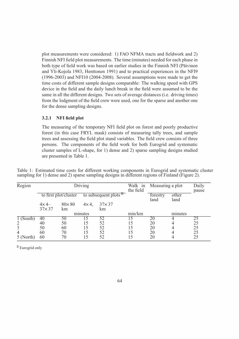
plot measurements were considered: 1) FAO NFMA tracts and eldwork and 2)

Finnish NFI eld plot measurements. The time (minutes) needed for each phase in

both type of eld work was based on earlier studies in the Finnish NFI (Päivinen

and Yli-Kojola 1983, Henttonen 1991) and to practical experiences in the NFI9

(1996-2003) and NFI10 (2004-2008). Several assumptions were made to get the

time costs of different sample designs comparable: The walking speed with GPS

device in the eld and the daily lunch break in the eld were assumed to be the

same in all the different designs. Two sets of average distances (i.e. driving times)

from the lodgment of the eld crew were used, one for the sparse and another one

for the dense sampling designs.

3.2.1 NFI eld plot

The measuring of the temporary NFI eld plot on forest and poorly productive

forest (in this case FRYL mask) consists of measuring tally trees, and sample

trees and assessing the eld plot stand variables. The eld crew consists of three

persons. The components of the eld work for both Eurogrid and systematic

cluster samples of L-shape, for 1) dense and 2) sparse sampling designs studied

are presented in Table 1.

Table 1: Estimated time costs for different working components in Eurogrid and systematic clustersampling for 1) dense and 2) sparse sampling designs in different regions of Finland (Figure 2).

Region Driving Walk inthe eld

Measuring a plot Dailypause

to rst plot/cluster to subsequent plots � forestryland

otherland

4× 4–37× 37

80× 80km

4× 4, 37× 37km

minutes min/km minutes1 (South) 40 50 15 52 15 20 4 252 40 50 15 52 15 20 4 253 50 60 15 52 15 20 4 254 60 70 15 52 15 20 4 255 (North) 60 70 15 52 15 20 4 25

� Eurogrid only

64

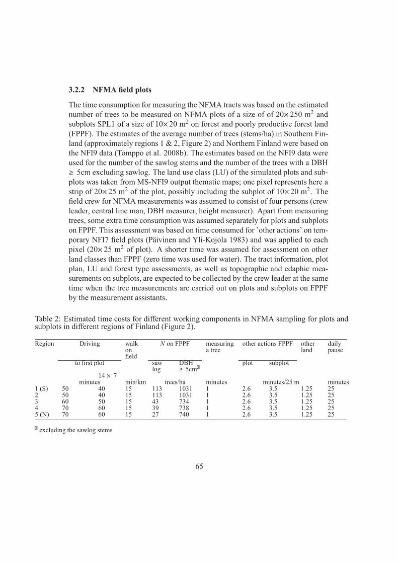
3.2.2 NFMA eld plots

The time consumption for measuring the NFMA tracts was based on the estimated

number of trees to be measured on NFMA plots of a size of of 20× 250 m2 and

subplots SPL1 of a size of 10× 20 m2 on forest and poorly productive forest land

(FPPF). The estimates of the average number of trees (stems/ha) in Southern Fin-

land (approximately regions 1 & 2, Figure 2) and Northern Finland were based on

the NFI9 data (Tomppo et al. 2008b). The estimates based on the NFI9 data were

used for the number of the sawlog stems and the number of the trees with a DBH

≥ 5cm excluding sawlog. The land use class (LU) of the simulated plots and sub-

plots was taken from MS-NFI9 output thematic maps; one pixel represents here a

strip of 20× 25 m2 of the plot, possibly including the subplot of 10× 20 m2. The

eld crew for NFMAmeasurements was assumed to consist of four persons (crew

leader, central line man, DBH measurer, height measurer). Apart from measuring

trees, some extra time consumption was assumed separately for plots and subplots

on FPPF. This assessment was based on time consumed for ’other actions’ on tem-

porary NFI7 eld plots (Päivinen and Yli-Kojola 1983) and was applied to each

pixel (20× 25 m2 of plot). A shorter time was assumed for assessment on other

land classes than FPPF (zero time was used for water). The tract information, plot

plan, LU and forest type assessments, as well as topographic and edaphic mea-

surements on subplots, are expected to be collected by the crew leader at the same

time when the tree measurements are carried out on plots and subplots on FPPF

by the measurement assistants.

Table 2: Estimated time costs for different working components in NFMA sampling for plots andsubplots in different regions of Finland (Figure 2).

Region Driving walkoneld

N on FPPF measuringa tree

other actions FPPF otherland

dailypause

to rst plot sawlog

DBH≥ 5cm�

plot subplot

14 × 7minutes min/km trees/ha minutes minutes/25 m minutes

1 (S) 50 40 15 113 1031 1 2.6 3.5 1.25 252 50 40 15 113 1031 1 2.6 3.5 1.25 253 60 50 15 43 734 1 2.6 3.5 1.25 254 70 60 15 39 738 1 2.6 3.5 1.25 255 (N) 70 60 15 27 740 1 2.6 3.5 1.25 25

� excluding the sawlog stems

65

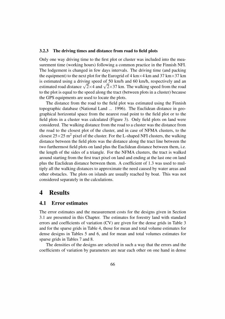
3.2.3 The driving times and distance from road to field plots

Only one way driving time to the first plot or cluster was included into the mea-

surement time (working hours) following a common practice in the Finnish NFI.

The lodgement is changed in few days intervals. The driving time (and packing

the equipment) to the next plot for the Eurogrid of 4 km×4 km and 37 km×37 km

is estimated using a driving speed of 50 km/h and 60 km/h, respectively and an

estimated road distance√

2×4 and√

2×37 km. The walking speed from the road

to the plot is equal to the speed along the tract (between plots in a cluster) because

the GPS equipments are used to locate the plots.

The distance from the road to the field plot was estimated using the Finnish

topographic database (National Land ... 1996). The Euclidean distance in geo-

graphical horizontal space from the nearest road point to the field plot or to the

field plots in a cluster was calculated (Figure 3). Only field plots on land were

considered. The walking distance from the road to a cluster was the distance from

the road to the closest plot of the cluster, and in case of NFMA clusters, to the

closest 25×25 m2 pixel of the cluster. For the L-shaped NFI clusters, the walking

distance between the field plots was the distance along the tract line between the

two furthermost field plots on land plus the Euclidean distance between them, i.e.

the length of the sides of a triangle. For the NFMA clusters, the tract is walked

around starting from the first tract pixel on land and ending at the last one on land

plus the Euclidean distance between them. A coefficient of 1.3 was used to mul-

tiply all the walking distances to approximate the need caused by water areas and

other obstacles. The plots on islands are usually reached by boat. This was not

considered separately in the calculations.

4 Results

4.1 Error estimates

The error estimates and the measurement costs for the designs given in Section

3.1 are presented in this Chapter. The estimates for forestry land with standard

errors and coefficients of variation (CV) are given for the dense grids in Table 3

and for the sparse grids in Table 4, those for mean and total volume estimates for

dense designs in Tables 5 and 6, and for mean and total volumes estimates for

sparse grids in Tables 7 and 8.

The densities of the designs are selected in such a way that the errors and the

coefficients of variation by parameters are near each other on one hand in dense

66

# # # # # #

#

#

#

#

#

#

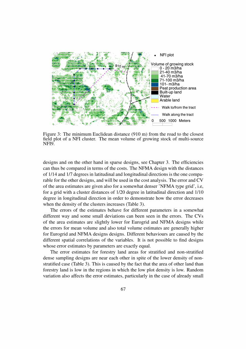
910 m Volume of growing stock0 - 20 m3/ha21-40 m3/ha 41-70 m3/ha71-100 m3/ha101- m3/haPeat production areaBuilt-up landWaterArable land

# NFI plot

Walk along the tract

Walk to/from the tract

0 500 1000 Meters

Figure 3: The minimum Euclidean distance (910 m) from the road to the closestfield plot of a NFI cluster. The mean volume of growing stock of multi-sourceNFI9.

designs and on the other hand in sparse designs, see Chapter 3. The efficiencies

can thus be compared in terms of the costs. The NFMA design with the distances

of 1/14 and 1/7 degrees in latitudinal and longitudinal directions is the one compa-

rable for the other designs, and will be used in the cost analysis. The error and CV

of the area estimates are given also for a somewhat denser ’NFMA type grid’, i.e,

for a grid with a cluster distances of 1/20 degree in latitudinal direction and 1/10

degree in longitudinal direction in order to demonstrate how the error decreases

when the density of the clusters increases (Table 3).

The errors of the estimates behave for different parameters in a somewhat

different way and some small deviations can been seen in the errors. The CVs

of the area estimates are slightly lower for Eurogrid and NFMA designs while

the errors for mean volume and also total volume estimates are generally higher

for Eurogrid and NFMA designs designs. Different behaviours are caused by the

different spatial correlations of the variables. It is not possible to find designs

whose error estimates by parameters are exactly equal.

The error estimates for forestry land areas for stratified and non-stratified

dense sampling designs are near each other in spite of the lower density of non-

stratified case (Table 3). This is caused by the fact that the area of other land than

forestry land is low in the regions in which the low plot density is low. Random

variation also affects the error estimates, particularly in the case of already small

67

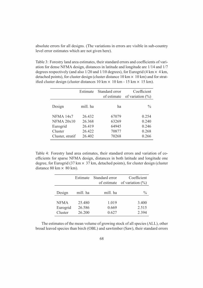
absolute errors for all designs. (The variations in errors are visible in sub-country

level error estimates which are not given here).

Table 3: Forestry land area estimates, their standard errors and coef cients of vari-

ation for dense NFMA design, distances in latitude and longitude are 1/14 and 1/7

degrees respectively (and also 1/20 and 1/10 degrees), for Eurogrid (4 km × 4 km,

detached points), for cluster design (cluster distance 10 km × 10 km) and for strat-

i ed cluster design (cluster distances 10 km × 10 km - 15 km × 15 km).

Estimate Standard error Coef cient

of estimate of variation (%)

Design mill. ha ha %

NFMA 14x7 26.432 67079 0.254

NFMA 20x10 26.368 63269 0.240

Eurogrid 26.419 64945 0.246

Cluster 26.422 70877 0.268

Cluster, stratif 26.402 70268 0.266

Table 4: Forestry land area estimates, their standard errors and variation of co-

ef cients for sparse NFMA design, distances in both latitude and longitude one

degree, for Eurogrid (37 km × 37 km, detached points), for cluster design (cluster

distance 80 km × 80 km).

Estimate Standard error Coef cient

of estimate of variation (%)

Design mill. ha mill. ha %

NFMA 25.480 1.019 3.400

Eurogrid 26.586 0.669 2.515

Cluster 26.200 0.627 2.394

The estimates of the mean volume of growing stock of all species (ALL), other

broad leaved species than birch (OBL) and sawtimber (Saw), their standard errors

68

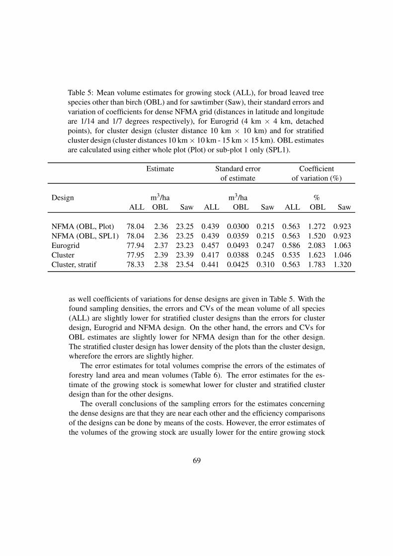
Table 5: Mean volume estimates for growing stock (ALL), for broad leaved tree

species other than birch (OBL) and for sawtimber (Saw), their standard errors and

variation of coefficients for dense NFMA grid (distances in latitude and longitude

are 1/14 and 1/7 degrees respectively), for Eurogrid (4 km × 4 km, detached

points), for cluster design (cluster distance 10 km × 10 km) and for stratified

cluster design (cluster distances 10 km × 10 km - 15 km × 15 km). OBL estimates

are calculated using either whole plot (Plot) or sub-plot 1 only (SPL1).

Estimate Standard error Coefficient

of estimate of variation (%)

Design m3/ha m3/ha %

ALL OBL Saw ALL OBL Saw ALL OBL Saw

NFMA (OBL, Plot) 78.04 2.36 23.25 0.439 0.0300 0.215 0.563 1.272 0.923

NFMA (OBL, SPL1) 78.04 2.36 23.25 0.439 0.0359 0.215 0.563 1.520 0.923

Eurogrid 77.94 2.37 23.23 0.457 0.0493 0.247 0.586 2.083 1.063

Cluster 77.95 2.39 23.39 0.417 0.0388 0.245 0.535 1.623 1.046

Cluster, stratif 78.33 2.38 23.54 0.441 0.0425 0.310 0.563 1.783 1.320

as well coefficients of variations for dense designs are given in Table 5. With the

found sampling densities, the errors and CVs of the mean volume of all species

(ALL) are slightly lower for stratified cluster designs than the errors for cluster

design, Eurogrid and NFMA design. On the other hand, the errors and CVs for

OBL estimates are slightly lower for NFMA design than for the other design.

The stratified cluster design has lower density of the plots than the cluster design,

wherefore the errors are slightly higher.

The error estimates for total volumes comprise the errors of the estimates of

forestry land area and mean volumes (Table 6). The error estimates for the es-

timate of the growing stock is somewhat lower for cluster and stratified cluster

design than for the other designs.

The overall conclusions of the sampling errors for the estimates concerning

the dense designs are that they are near each other and the efficiency comparisons

of the designs can be done by means of the costs. However, the error estimates of

the volumes of the growing stock are usually lower for the entire growing stock

69

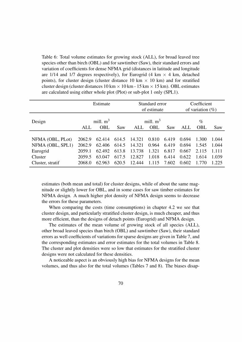
Table 6: Total volume estimates for growing stock (ALL), for broad leaved tree

species other than birch (OBL) and for sawtimber (Saw), their standard errors and

variation of coefficients for dense NFMA grid (distances in latitude and longitude

are 1/14 and 1/7 degrees respectively), for Eurogrid (4 km × 4 km, detached

points), for cluster design (cluster distance 10 km × 10 km) and for stratified

cluster design (cluster distances 10 km × 10 km - 15 km × 15 km). OBL estimates

are calculated using either whole plot (Plot) or sub-plot 1 only (SPL1).

Estimate Standard error Coefficient

of estimate of variation (%)

Design mill. m3 mill. m3 %

ALL OBL Saw ALL OBL Saw ALL OBL Saw

NFMA (OBL, PLot) 2062.9 62.414 614.5 14.321 0.810 6.419 0.694 1.300 1.044

NFMA (OBL, SPL1) 2062.9 62.406 614.5 14.321 0.964 6.419 0.694 1.545 1.044

Eurogrid 2059.1 62.492 613.8 13.738 1.321 6.817 0.667 2.115 1.111

Cluster 2059.5 63.047 617.5 12.827 1.018 6.414 0.622 1.614 1.039

Cluster, stratif 2068.0 62.963 620.5 12.444 1.115 7.602 0.602 1.770 1.225

estimates (both mean and total) for cluster designs, while of about the same mag-

nitude or slightly lower for OBL, and in some cases for saw timber estimates for

NFMA design. A much higher plot density of NFMA design seems to decrease

the errors for these parameters.

When comparing the costs (time consumptions) in chapter 4.2 we see that

cluster design, and particularly stratified cluster design, is much cheaper, and thus

more efficient, than the designs of detach points (Eurogrid) and NFMA design.

The estimates of the mean volume of growing stock of all species (ALL),

other broad leaved species than birch (OBL) and sawtimber (Saw), their standard

errors as well coefficients of variations for sparse designs are given in Table 7, and

the corresponding estimates and error estimates for the total volumes in Table 8.

The cluster and plot densities were so low that estimates for the stratified cluster

designs were not calculated for these densities.

A noticeable aspect is an obviously high bias for NFMA designs for the mean

volumes, and thus also for the total volumes (Tables 7 and 8). The biases disap-

70

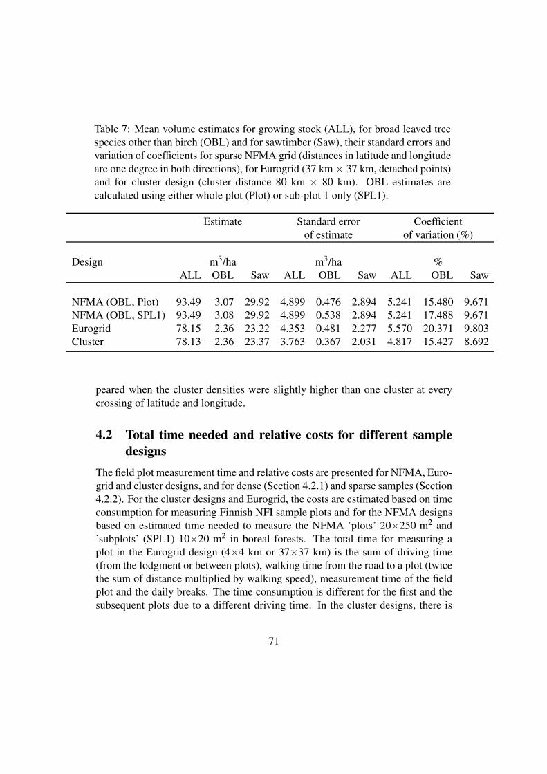
Table 7: Mean volume estimates for growing stock (ALL), for broad leaved tree

species other than birch (OBL) and for sawtimber (Saw), their standard errors and

variation of coefficients for sparse NFMA grid (distances in latitude and longitude

are one degree in both directions), for Eurogrid (37 km × 37 km, detached points)

and for cluster design (cluster distance 80 km × 80 km). OBL estimates are

calculated using either whole plot (Plot) or sub-plot 1 only (SPL1).

Estimate Standard error Coefficient

of estimate of variation (%)

Design m3/ha m3/ha %

ALL OBL Saw ALL OBL Saw ALL OBL Saw

NFMA (OBL, Plot) 93.49 3.07 29.92 4.899 0.476 2.894 5.241 15.480 9.671

NFMA (OBL, SPL1) 93.49 3.08 29.92 4.899 0.538 2.894 5.241 17.488 9.671

Eurogrid 78.15 2.36 23.22 4.353 0.481 2.277 5.570 20.371 9.803

Cluster 78.13 2.36 23.37 3.763 0.367 2.031 4.817 15.427 8.692

peared when the cluster densities were slightly higher than one cluster at every

crossing of latitude and longitude.

4.2 Total time needed and relative costs for different sample

designs

The field plot measurement time and relative costs are presented for NFMA, Euro-

grid and cluster designs, and for dense (Section 4.2.1) and sparse samples (Section

4.2.2). For the cluster designs and Eurogrid, the costs are estimated based on time

consumption for measuring Finnish NFI sample plots and for the NFMA designs

based on estimated time needed to measure the NFMA ’plots’ 20×250 m2 and

’subplots’ (SPL1) 10×20 m2 in boreal forests. The total time for measuring a

plot in the Eurogrid design (4×4 km or 37×37 km) is the sum of driving time

(from the lodgment or between plots), walking time from the road to a plot (twice

the sum of distance multiplied by walking speed), measurement time of the field

plot and the daily breaks. The time consumption is different for the first and the

subsequent plots due to a different driving time. In the cluster designs, there is

71

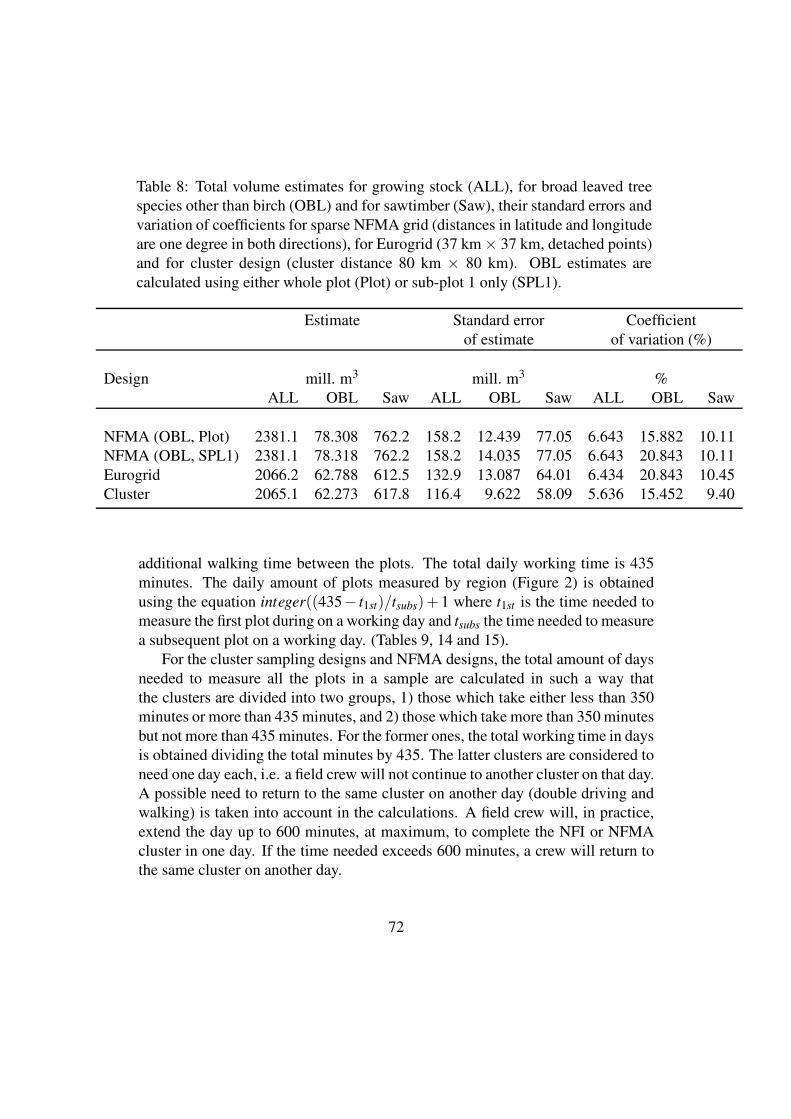
Table 8: Total volume estimates for growing stock (ALL), for broad leaved tree

species other than birch (OBL) and for sawtimber (Saw), their standard errors and

variation of coefficients for sparse NFMA grid (distances in latitude and longitude

are one degree in both directions), for Eurogrid (37 km × 37 km, detached points)

and for cluster design (cluster distance 80 km × 80 km). OBL estimates are

calculated using either whole plot (Plot) or sub-plot 1 only (SPL1).

Estimate Standard error Coefficient

of estimate of variation (%)

Design mill. m3 mill. m3 %

ALL OBL Saw ALL OBL Saw ALL OBL Saw

NFMA (OBL, Plot) 2381.1 78.308 762.2 158.2 12.439 77.05 6.643 15.882 10.11

NFMA (OBL, SPL1) 2381.1 78.318 762.2 158.2 14.035 77.05 6.643 20.843 10.11

Eurogrid 2066.2 62.788 612.5 132.9 13.087 64.01 6.434 20.843 10.45

Cluster 2065.1 62.273 617.8 116.4 9.622 58.09 5.636 15.452 9.40

additional walking time between the plots. The total daily working time is 435

minutes. The daily amount of plots measured by region (Figure 2) is obtained

using the equation integer((435− t1st)/tsubs)+1 where t1st is the time needed to

measure the first plot during on a working day and tsubs the time needed to measure

a subsequent plot on a working day. (Tables 9, 14 and 15).

For the cluster sampling designs and NFMA designs, the total amount of days

needed to measure all the plots in a sample are calculated in such a way that

the clusters are divided into two groups, 1) those which take either less than 350

minutes or more than 435 minutes, and 2) those which take more than 350 minutes

but not more than 435 minutes. For the former ones, the total working time in days

is obtained dividing the total minutes by 435. The latter clusters are considered to

need one day each, i.e. a field crew will not continue to another cluster on that day.

A possible need to return to the same cluster on another day (double driving and

walking) is taken into account in the calculations. A field crew will, in practice,

extend the day up to 600 minutes, at maximum, to complete the NFI or NFMA

cluster in one day. If the time needed exceeds 600 minutes, a crew will return to

the same cluster on another day.

72

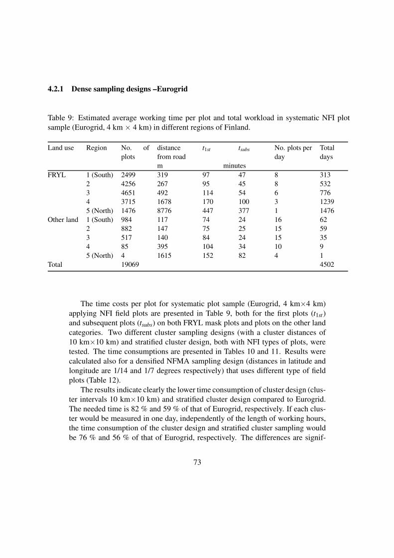
4.2.1 Dense sampling designs –Eurogrid

Table 9: Estimated average working time per plot and total workload in systematic NFI plot

sample (Eurogrid, 4 km × 4 km) in different regions of Finland.

Land use Region No. of

plots

distance

from road

t1st tsubs No. plots per

day

Total

days

m minutes

FRYL 1 (South) 2499 319 97 47 8 313

2 4256 267 95 45 8 532

3 4651 492 114 54 6 776

4 3715 1678 170 100 3 1239

5 (North) 1476 8776 447 377 1 1476

Other land 1 (South) 984 117 74 24 16 62

2 882 147 75 25 15 59

3 517 140 84 24 15 35

4 85 395 104 34 10 9

5 (North) 4 1615 152 82 4 1

Total 19069 4502

The time costs per plot for systematic plot sample (Eurogrid, 4 km×4 km)

applying NFI field plots are presented in Table 9, both for the first plots (t1st)

and subsequent plots (tsubs) on both FRYL mask plots and plots on the other land

categories. Two different cluster sampling designs (with a cluster distances of

10 km×10 km) and stratified cluster design, both with NFI types of plots, were

tested. The time consumptions are presented in Tables 10 and 11. Results were

calculated also for a densified NFMA sampling design (distances in latitude and

longitude are 1/14 and 1/7 degrees respectively) that uses different type of field

plots (Table 12).

The results indicate clearly the lower time consumption of cluster design (clus-

ter intervals 10 km×10 km) and stratified cluster design compared to Eurogrid.

The needed time is 82 % and 59 % of that of Eurogrid, respectively. If each clus-

ter would be measured in one day, independently of the length of working hours,

the time consumption of the cluster design and stratified cluster sampling would

be 76 % and 56 % of that of Eurogrid, respectively. The differences are signif-

73

Table 10: Estimated average working time (t) per cluster and total workload in systematic cluster sampling

of 10×10 km and 12 NFI plots per cluster in different regions of Finland.

Region No. of

clusters

No. of

plots

distance

from road

cluster Total days

t < 350 min. or

t > 435 min.

350 min. < t <

435 min.

All

m minutes

1 (South) 693 6693 374 338 256 316 572

2 969 9723 93 348 226 601 827

3 929 10133 123 394 456 418 864

4 629 7165 1095 496 564 161 725

5 (North) 277 2883 7928 1117 684 30 714

3497 36597 957 445 3712

icant, especially in Northern Finland (Lapland), regions 4 and 5, where the road

network is sparse.

A large number of NFMA clusters were needed (6228) to achieve the same

error level as the other designs. The relative time consumption was 171 % of that

of Eurogrid and 288 % of the stratified cluster design and 208 % of (unstratified)

cluster design. Relative costs of densified NFMA are even higher when we take

into account the assumed size of field crew 1+3 persons versus 1+2 for the other

designs. Approximating the increase in salaries and other costs by a coefficient of

1.29 for NFMA, the relative cost of NFMA would be 220 % of that of Eurogrid

and 372 % of the stratified cluster design.

The comparison is done based on the assumption that the country level stan-

dard errors of the estimates for variables of interest are approximately of the same

magnitude in all sample designs.

It should be noted that the optimal cluster size should be, in practice, smaller in

Northern Finland than in Southern Finland, because the average time cost clearly

exceeds the 435 minutes daily working time in the North due to long walking and

driving distances. The driving costs paid to the car owner in a field crew would

be higher in the Eurogrid design than in the other designs. On the other hand, it

is possible that a field crew has to change the lodging more often in the cluster

74

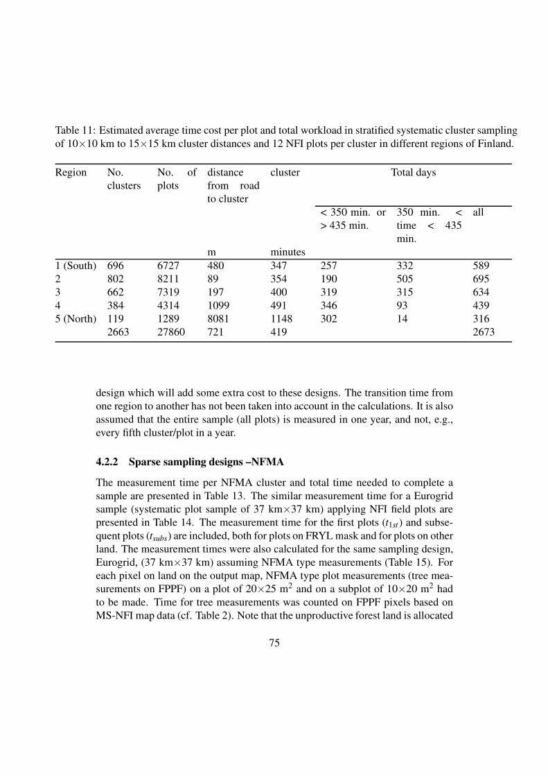
Table 11: Estimated average time cost per plot and total workload in stratified systematic cluster sampling

of 10×10 km to 15×15 km cluster distances and 12 NFI plots per cluster in different regions of Finland.

Region No.

clusters

No. of

plots

distance

from road

to cluster

cluster Total days

< 350 min. or

> 435 min.

350 min. <

time < 435

min.

all

m minutes

1 (South) 696 6727 480 347 257 332 589

2 802 8211 89 354 190 505 695

3 662 7319 197 400 319 315 634

4 384 4314 1099 491 346 93 439

5 (North) 119 1289 8081 1148 302 14 316

2663 27860 721 419 2673

design which will add some extra cost to these designs. The transition time from

one region to another has not been taken into account in the calculations. It is also

assumed that the entire sample (all plots) is measured in one year, and not, e.g.,

every fifth cluster/plot in a year.

4.2.2 Sparse sampling designs –NFMA

The measurement time per NFMA cluster and total time needed to complete a

sample are presented in Table 13. The similar measurement time for a Eurogrid

sample (systematic plot sample of 37 km×37 km) applying NFI field plots are

presented in Table 14. The measurement time for the first plots (t1st) and subse-

quent plots (tsubs) are included, both for plots on FRYL mask and for plots on other

land. The measurement times were also calculated for the same sampling design,

Eurogrid, (37 km×37 km) assuming NFMA type measurements (Table 15). For

each pixel on land on the output map, NFMA type plot measurements (tree mea-

surements on FPPF) on a plot of 20×25 m2 and on a subplot of 10×20 m2 had

to be made. Time for tree measurements was counted on FPPF pixels based on

MS-NFI map data (cf. Table 2). Note that the unproductive forest land is allocated

75

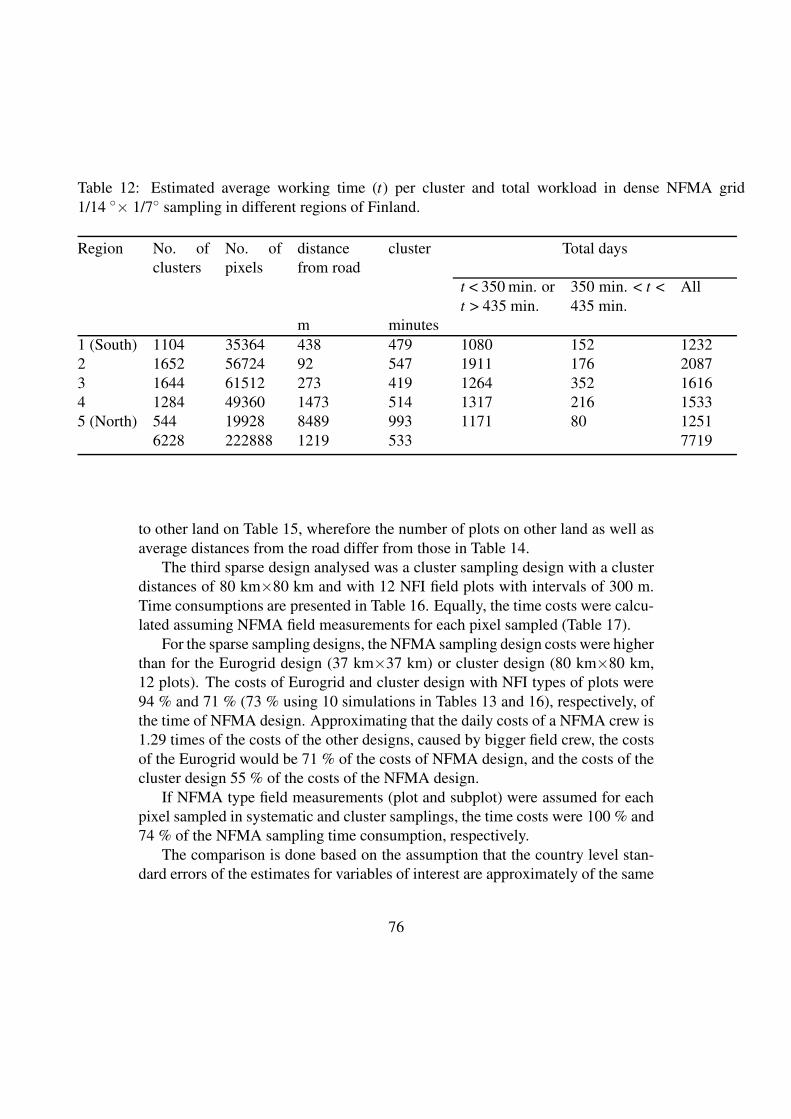
Table 12: Estimated average working time (t) per cluster and total workload in dense NFMA grid

1/14 ◦× 1/7◦ sampling in different regions of Finland.

Region No. of

clusters

No. of

pixels

distance

from road

cluster Total days

t < 350 min. or

t > 435 min.

350 min. < t <

435 min.

All

m minutes

1 (South) 1104 35364 438 479 1080 152 1232

2 1652 56724 92 547 1911 176 2087

3 1644 61512 273 419 1264 352 1616

4 1284 49360 1473 514 1317 216 1533

5 (North) 544 19928 8489 993 1171 80 1251

6228 222888 1219 533 7719

to other land on Table 15, wherefore the number of plots on other land as well as

average distances from the road differ from those in Table 14.

The third sparse design analysed was a cluster sampling design with a cluster

distances of 80 km×80 km and with 12 NFI field plots with intervals of 300 m.

Time consumptions are presented in Table 16. Equally, the time costs were calcu-

lated assuming NFMA field measurements for each pixel sampled (Table 17).

For the sparse sampling designs, the NFMA sampling design costs were higher

than for the Eurogrid design (37 km×37 km) or cluster design (80 km×80 km,

12 plots). The costs of Eurogrid and cluster design with NFI types of plots were

94 % and 71 % (73 % using 10 simulations in Tables 13 and 16), respectively, of

the time of NFMA design. Approximating that the daily costs of a NFMA crew is

1.29 times of the costs of the other designs, caused by bigger field crew, the costs

of the Eurogrid would be 71 % of the costs of NFMA design, and the costs of the

cluster design 55 % of the costs of the NFMA design.

If NFMA type field measurements (plot and subplot) were assumed for each

pixel sampled in systematic and cluster samplings, the time costs were 100 % and

74 % of the NFMA sampling time consumption, respectively.

The comparison is done based on the assumption that the country level stan-

dard errors of the estimates for variables of interest are approximately of the same

76

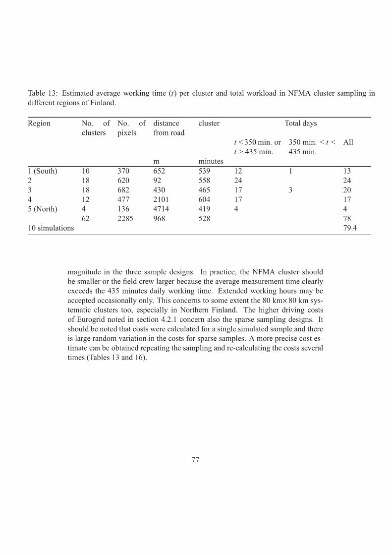
Table 13: Estimated average working time (t) per cluster and total workload in NFMA cluster sampling in

different regions of Finland.

Region No. of

clusters

No. of

pixels

distance

from road

cluster Total days

t < 350 min. or

t > 435 min.

350 min. < t <

435 min.

All

m minutes

1 (South) 10 370 652 539 12 1 13

2 18 620 92 558 24 24

3 18 682 430 465 17 3 20

4 12 477 2101 604 17 17

5 (North) 4 136 4714 419 4 4

62 2285 968 528 78

10 simulations 79.4

magnitude in the three sample designs. In practice, the NFMA cluster should

be smaller or the eld crew larger because the average measurement time clearly

exceeds the 435 minutes daily working time. Extended working hours may be

accepted occasionally only. This concerns to some extent the 80 km× 80 km sys-

tematic clusters too, especially in Northern Finland. The higher driving costs

of Eurogrid noted in section 4.2.1 concern also the sparse sampling designs. It

should be noted that costs were calculated for a single simulated sample and there

is large random variation in the costs for sparse samples. A more precise cost es-

timate can be obtained repeating the sampling and re-calculating the costs several

times (Tables 13 and 16).

77

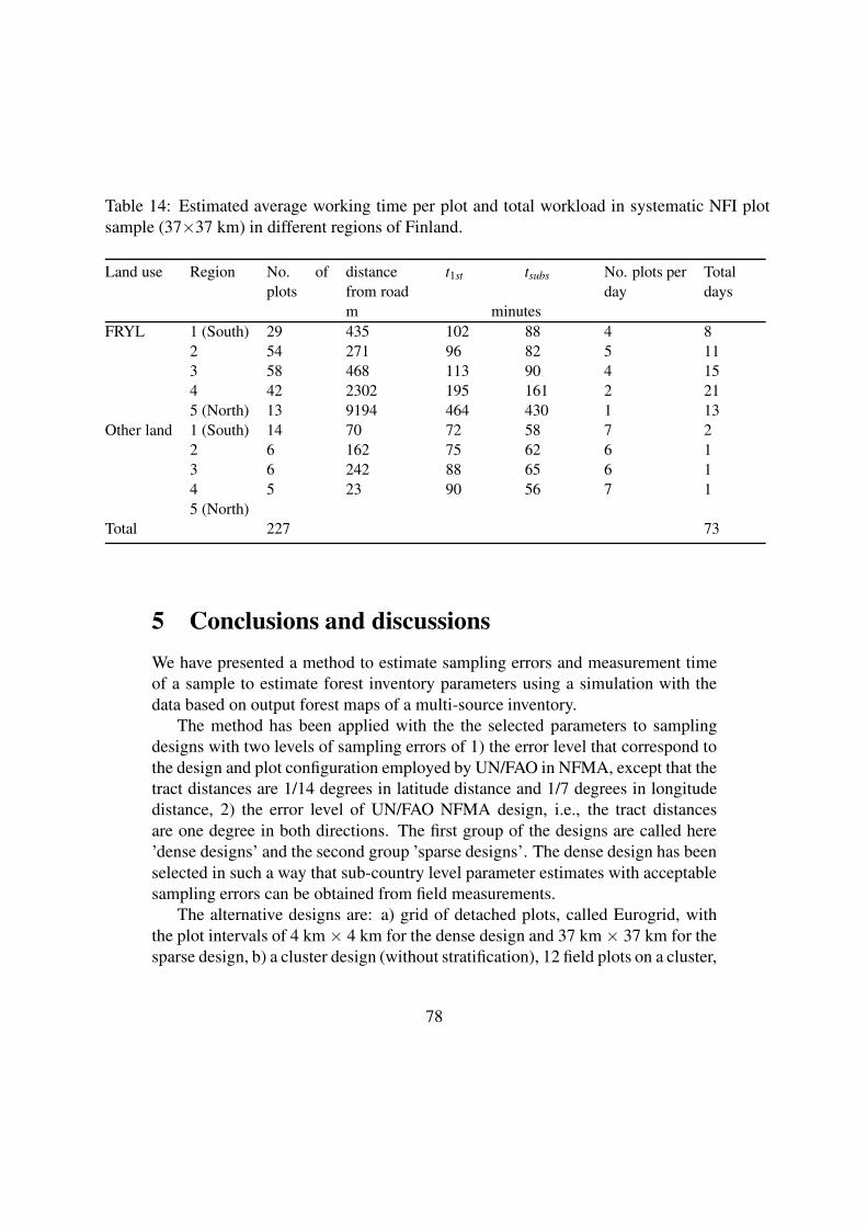
Table 14: Estimated average working time per plot and total workload in systematic NFI plot

sample (37×37 km) in different regions of Finland.

Land use Region No. of

plots

distance

from road

t1st tsubs No. plots per

day

Total

days

m minutes

FRYL 1 (South) 29 435 102 88 4 8

2 54 271 96 82 5 11

3 58 468 113 90 4 15

4 42 2302 195 161 2 21

5 (North) 13 9194 464 430 1 13

Other land 1 (South) 14 70 72 58 7 2

2 6 162 75 62 6 1

3 6 242 88 65 6 1

4 5 23 90 56 7 1

5 (North)

Total 227 73

5 Conclusions and discussions

We have presented a method to estimate sampling errors and measurement time

of a sample to estimate forest inventory parameters using a simulation with the

data based on output forest maps of a multi-source inventory.

The method has been applied with the the selected parameters to sampling

designs with two levels of sampling errors of 1) the error level that correspond to

the design and plot configuration employed by UN/FAO in NFMA, except that the

tract distances are 1/14 degrees in latitude distance and 1/7 degrees in longitude

distance, 2) the error level of UN/FAO NFMA design, i.e., the tract distances

are one degree in both directions. The first group of the designs are called here

’dense designs’ and the second group ’sparse designs’. The dense design has been

selected in such a way that sub-country level parameter estimates with acceptable

sampling errors can be obtained from field measurements.

The alternative designs are: a) grid of detached plots, called Eurogrid, with

the plot intervals of 4 km × 4 km for the dense design and 37 km × 37 km for the

sparse design, b) a cluster design (without stratification), 12 field plots on a cluster,

78

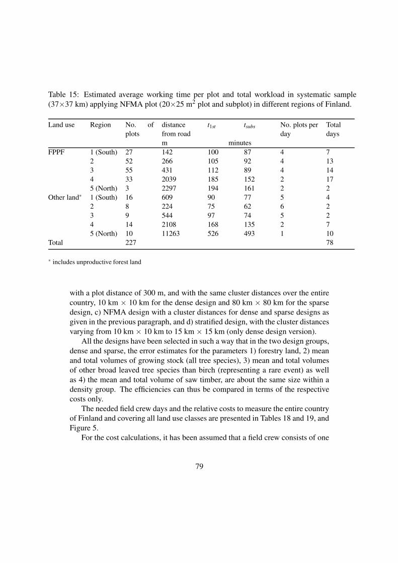
Table 15: Estimated average working time per plot and total workload in systematic sample

(37×37 km) applying NFMA plot (20×25 m2 plot and subplot) in different regions of Finland.

Land use Region No. of

plots

distance

from road

t1st tsubs No. plots per

day

Total

days

m minutes

FPPF 1 (South) 27 142 100 87 4 7

2 52 266 105 92 4 13

3 55 431 112 89 4 14

4 33 2039 185 152 2 17

5 (North) 3 2297 194 161 2 2

Other land∗ 1 (South) 16 609 90 77 5 4

2 8 224 75 62 6 2

3 9 544 97 74 5 2

4 14 2108 168 135 2 7

5 (North) 10 11263 526 493 1 10

Total 227 78

∗ includes unproductive forest land

with a plot distance of 300 m, and with the same cluster distances over the entire

country, 10 km × 10 km for the dense design and 80 km × 80 km for the sparse

design, c) NFMA design with a cluster distances for dense and sparse designs as

given in the previous paragraph, and d) stratified design, with the cluster distances

varying from 10 km × 10 km to 15 km × 15 km (only dense design version).

All the designs have been selected in such a way that in the two design groups,

dense and sparse, the error estimates for the parameters 1) forestry land, 2) mean

and total volumes of growing stock (all tree species), 3) mean and total volumes

of other broad leaved tree species than birch (representing a rare event) as well

as 4) the mean and total volume of saw timber, are about the same size within a

density group. The efficiencies can thus be compared in terms of the respective

costs only.

The needed field crew days and the relative costs to measure the entire country

of Finland and covering all land use classes are presented in Tables 18 and 19, and

Figure 5.

For the cost calculations, it has been assumed that a field crew consists of one

79

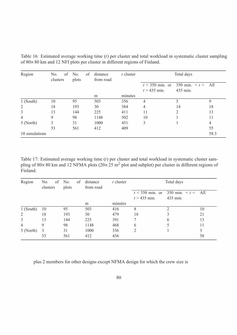
Table 16: Estimated average working time (t) per cluster and total workload in systematic cluster sampling

of 80× 80 km and 12 NFI plots per cluster in different regions of Finland.

Region No. of

clusters

No. of

plots

distance

from road

t cluster Total days

t < 350 min. or

t > 435 min.

350 min. < t <

435 min.

All

m minutes

1 (South) 10 95 503 356 4 5 9

2 18 193 30 384 4 14 18

3 13 144 225 411 11 2 13

4 9 98 1148 502 10 1 11

5 (North) 3 31 1000 451 3 1 4

53 561 412 409 55

10 simulations 58.3

Table 17: Estimated average working time (t) per cluster and total workload in systematic cluster sam-

pling of 80× 80 km and 12 NFMA plots (20× 25 m2 plot and subplot) per cluster in different regions of

Finland.

Region No. of

clusters

No. of

plots

distance

from road

t cluster Total days

t < 350 min. or

t > 435 min.

350 min. < t <

435 min.

All

m minutes

1 (South) 10 95 503 416 8 2 10

2 18 193 30 479 18 3 21

3 13 144 225 391 7 6 13

4 9 98 1148 468 6 5 11

5 (North) 3 31 1000 336 2 1 3

53 561 412 436 58

plus 2 members for other designs except NFMA design for which the crew size is

80

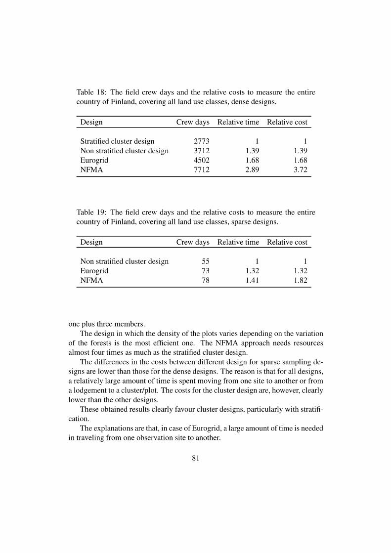
Table 18: The field crew days and the relative costs to measure the entire

country of Finland, covering all land use classes, dense designs.

Design Crew days Relative time Relative cost

Stratified cluster design 2773 1 1

Non stratified cluster design 3712 1.39 1.39

Eurogrid 4502 1.68 1.68

NFMA 7712 2.89 3.72

Table 19: The field crew days and the relative costs to measure the entire

country of Finland, covering all land use classes, sparse designs.

Design Crew days Relative time Relative cost

Non stratified cluster design 55 1 1

Eurogrid 73 1.32 1.32

NFMA 78 1.41 1.82

one plus three members.

The design in which the density of the plots varies depending on the variation

of the forests is the most efficient one. The NFMA approach needs resources

almost four times as much as the stratified cluster design.

The differences in the costs between different design for sparse sampling de-

signs are lower than those for the dense designs. The reason is that for all designs,

a relatively large amount of time is spent moving from one site to another or from

a lodgement to a cluster/plot. The costs for the cluster design are, however, clearly

lower than the other designs.

These obtained results clearly favour cluster designs, particularly with stratifi-

cation.

The explanations are that, in case of Eurogrid, a large amount of time is needed

in traveling from one observation site to another.

81

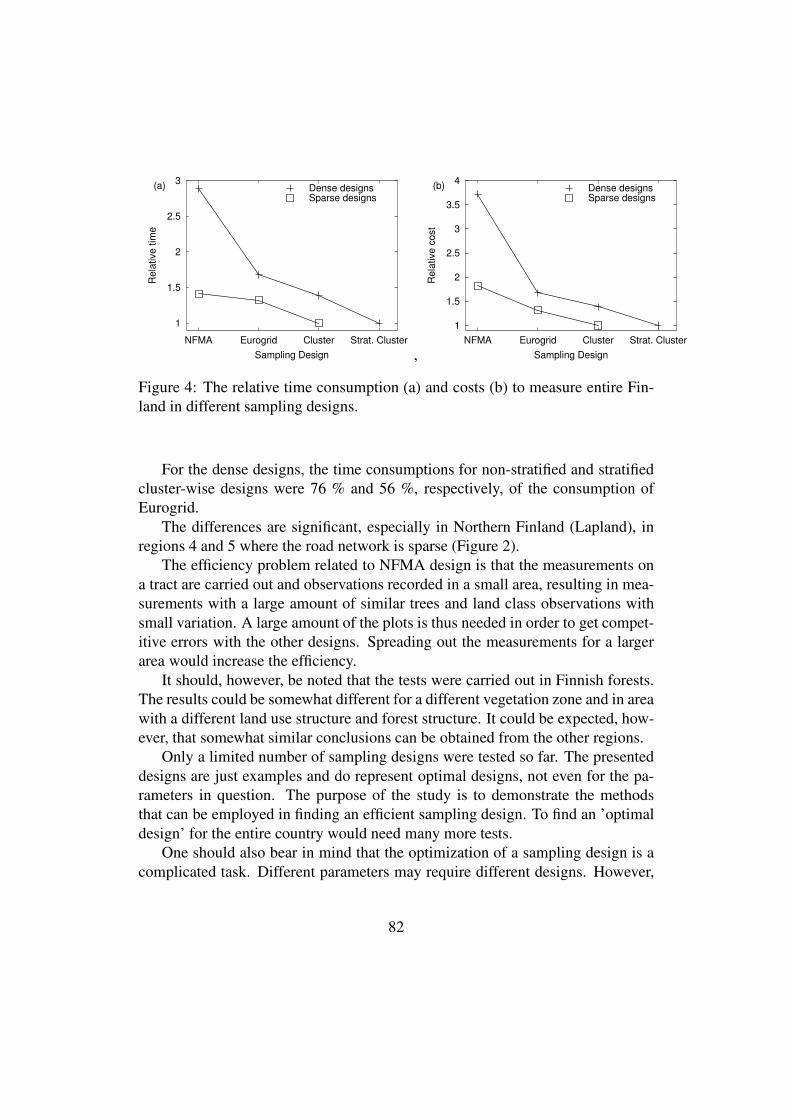
1

1.5

2

2.5

3

NFMA Eurogrid Cluster Strat. Cluster

Rela

tive tim

e

Sampling Design

(a) Dense designsSparse designs

,

1

1.5

2

2.5

3

3.5

4

NFMA Eurogrid Cluster Strat. Cluster

Rela

tive c

ost

Sampling Design

(b) Dense designsSparse designs

Figure 4: The relative time consumption (a) and costs (b) to measure entire Fin-

land in different sampling designs.

For the dense designs, the time consumptions for non-stratified and stratified

cluster-wise designs were 76 % and 56 %, respectively, of the consumption of

Eurogrid.

The differences are significant, especially in Northern Finland (Lapland), in

regions 4 and 5 where the road network is sparse (Figure 2).

The efficiency problem related to NFMA design is that the measurements on

a tract are carried out and observations recorded in a small area, resulting in mea-

surements with a large amount of similar trees and land class observations with

small variation. A large amount of the plots is thus needed in order to get compet-

itive errors with the other designs. Spreading out the measurements for a larger

area would increase the efficiency.

It should, however, be noted that the tests were carried out in Finnish forests.

The results could be somewhat different for a different vegetation zone and in area

with a different land use structure and forest structure. It could be expected, how-

ever, that somewhat similar conclusions can be obtained from the other regions.

Only a limited number of sampling designs were tested so far. The presented

designs are just examples and do represent optimal designs, not even for the pa-

rameters in question. The purpose of the study is to demonstrate the methods

that can be employed in finding an efficient sampling design. To find an ’optimal

design’ for the entire country would need many more tests.

One should also bear in mind that the optimization of a sampling design is a

complicated task. Different parameters may require different designs. However,

82

the tested basic parameters should give a good picture also for other parameters.

All the results should be considered as preliminary, and the work will be con-

tinued. However, we believe that a similar study can be extended outside of Fin-

land, and also using other type of forest, land use and land cover data presented in

a map form.

83

REFERENCES

Cressie (1991). Statistics for spatial data. Wiley, New York.

Diemer, C., Lucaschewski, I., Spelsberg, G., Tomppo, E., & Pekkarinen, A. (2000).

Integration of terrestrial forest sample plot data, map information and satellite

data. An operational multisource-inventory concept. In: Ranchin, T. & Wald,

L. (Eds.), Proceedings of the Third Conference "Fusion of Earth Data: Merg-

ing Point Measurements, Raster Maps and Remotely Sensed Images" January

26-28, 2000. Sophia Antipolis, France. SEE/URISCA, Nice (pp. 143-150).

FAO. 2004. National Forest Inventory Field Manual Template. Rome, August

2004. ftp://ftp.fao.org/docrep/fao/008/ae578e/ae578e00.pdf.

FAO. 2008. National Forest Monitoring and Assessment - NFMA.

http://www.fao.org/forestry/47655/en/

Gregoire, T. G. & Valentine, H.T. (2008). Sampling strategies for natural re-

sources and the environment. Chapman & Hall/CRC, Applied Environmental

Statistics. Boca Raton. 474 p. ISBN 978-1-58488-370-8.

Halme, M., & Tomppo, E. (2001). Improving the accuracy of multisource forest

inventory estimates by reducing plot location error - a multicriteria approach.

Remote Sensing of Environment, 78, 321-327.

Henttonen H. 1991. VMI8:n Pohjois-Suomen otanta-asetelmien vertailu satelliit-

tikuvatulkinnan avulla. (Comparisons of sampling designs for NFI8 in North

Finland.) Finnish Forest Research Institute, Manuscript, in Finnish.

Katila, M. & Tomppo, E. (2001). Selecting estimation parameters for the Finnish

multisource National Forest Inventory. Remote Sensing of Environment, 76,

16-32.

Katila, M. & Tomppo, E. (2006). Sampling simulation on multi-source output for-

est maps – an application for small areas. In: M. Caetano & M. Painho (ed.),

Proceedings of 7th International Symposium on Spatial Accuracy Assessment

in Natural Resources and Environmental Sciences, 5–7 July 2006, Lissabon,

Portugal. Instituto Geográfico Português, Lissabon. ISBN 972-8867-27-1, p.

614-623. http://spatial-accuracy.org/2006/PDF/Katila2006accuracy.pdf.

Matérn, B. (1960). Spatial variation. Meddelanden fran Statens Skogsforskn-

ingsinstitut, 49, 5.

McRoberts, R. E., Nelson, M. D., & Wendt, D. G. (2002). Stratified estimation of

forest area using satellite imagery, inventory data, and the k-Nearest Neigh-

bors technique. Remote Sensing of Environment, 82, 457-468.

84

National Land Survey of Finland. 1996. Maastotietojen kohdemalli, Feature cat-

alog of the topographic database. Maanmittauslaitoksen julkaisuja 71. Na-

tional Land Survey of Finland. (in Finnish).

Nieschulze, J., & Sabrowski, F. (2003). Regionalisation of Point Information: A

Comparison of Parameter Estimation Techniques for Universal Kriging.

http://cms1.gre.ac.uk/conferences/iufro/proceedings/Niesc hiszeSaborawski1.pdf.

In: K. Rennolls (Ed.): Proceedings of IUFRO 4.11 Conference: Forest Biom-

etry, Modelling and Information Science. University of Greenwich, June

2001.

http://cms1.gre.ac.uk/conferences/iufro/proceedings/

Nilsson, M. (1997). Estimation of forest variables using satellite image data and

airborne lidar. Ph.D. thesis, Swedish University of Agricultural Sciences, The

Department of Forest Resource Management and Geomatics. Acta Universi-

tatis Agriculturae Sueciae. Silvestria, 17.

Päivinen, R. and Yli-Kojola H. 1083. Valtakunnan metsien inventoinnin ajankäyttö.

(Time consumtion in different measuring phase in NFI.) Finnish Forest Re-

search Institute, Manuscript, in Finnish.

Stein, M. (1999), Interpolation of Spatial Data: Some Theory for Kriging, Springer.

Taskinen, I. and Heikkinen, J. (2004): A nonparametric Bayesian method for as-

sessing uncertainty in thematic maps of forest variables. Revision submitted

to Journal of Agricultural, Biological, and Environmental Statistics.

Tomppo, E. (2006a). The Finnish National Forest Inventory. In: Kangas, A. &

Maltamo, M. (eds.). Forest inventory. Methodology and applications. Man-

aging Forest Ecosystems. Vol 10. Springer, Dordrecht. p. 179-194.

Tomppo, E. (1996b). Multi-source National Forest Inventory of Finland. In: R.

Vanclay, J. Vanclay, & S. Miina (Eds.), New Thrusts in Forest Inventory. Pro-

ceedings of the Subject Group S4.02-00 ‘Forest Resource Inventory and Mon-

itoring’ and Subject Group S4.12-00 ‘Remote Sensing Technology’. vol. 1.

IUFRO XX World Congress 6-12 Aug. 1995, (pp. 27-41) Tampere, Finland.

EFI Proceedings, 7. European Forest Institute. Joensuu. Finland.

Tomppo E., Goulding C., & Katila M. (1999). Adapting Finnish multi-source

forest inventory techniques to the New Zealand preharvest inventory. Scandi-

navian Journal of Forest Research, 14, 182-192.

Tomppo, E., Korhonen, K.T., Heikkinen, J., & Yli-Kojola, H. (2001a). Multi-

source inventory of the forests of the Hebei Forestry Bureau, Heilongjiang,

China. Silva Fennica, 35, 309-328.

Tomppo, E. & Halme, M. (2004). Using coarse scale forest variables as ancil-

85

lary information and weighting of variables in k-NN estimation - a genetic

algorithm approach. Remote Sensing of Environment, 92, 1-20.

Tomppo, E., Haakana, M., Katila, M., & Peräsaari, J. (2008a). Multi-Source

National Forest Inventory Methods and Applications Series: Managing Forest

Ecosystems , Vol. 18. XIV, 374 p. 22 illus. in color., Hardcover. ISBN: 978-

1-4020-8712-7. Online version available

Tomppo, E., Heikkinen, J., Tuomainen, T., Ihalainen, A., Mäkelä, H. & Tonteri, T.

(2008b). The 9th National Forest Inventory of Finland. Methods and Results.

Finnish Forest Research Institute. Manuscript.

UN-ECE/FAO. (2000). Forest Resources of Europe,CIS, North America, Aus-

tralia, Japan and New Zealand. United Nations, New York and Geneva, 2000.

86