Proceedings: Building Simulation 2007

- 629 -

TECHNIQUE OF UNCERTAINTY AND SENSITIVITY ANALYSIS FOR SUSTAINABLE BUILDING ENERGY SYSTEMS PERFORMANCE

CALCULATIONS

Kotek Petr1.1, Jordán Filip1, Kabele Karel1, Hensen Jan2

1Department of Microenvironmental and Building Services Engineering, CTU Technical University in Prague, Czech Republic

2Building Physics & Systems, Technische Universiteit Eindhoven, Netherlands 1.1contact: kotek.petr@centrum.cz

ABSTRACT Sustainable buildings design process is typical for modeling and simulation usage. The main reason is because there is generally no experience with such buildings and there is lot of new approaches and technical solutions to be used. Computer simulation could be supporting tool in engineering design process and can bring the good way for reducing energy consumption together with optimalization algorithm. For the optimization process we have to know which most sensitive input parametr from many of them has to be investigate. Therefore at first is necessary to perform the sensitivity analysis and find out the “strongest” input parametrs which most affecting the results under observation. Also still the simulation tools are mainly using to predict energy consumption, boiler and chiller loads, indor air quality, etc. before the building is build. The information about the building envelope, schedule and HVAC components are unclear and can bring large uncertainty in results by setting this inputs to the simulation tools. Paper presents preview of uncertainty and sensitivity analysis. This techniques are shown on case study concretely BESTEST case600 with DRYCOLD climate conditions. Also systems VAV (variable volume of air) and water fan-coil system are compared. For this prototype the simulation tool IES <Virtual Environment> was chosen.

KEYWORDS uncertainty and sensitivity analysis, MonteCarlo, Latin Hypercube sampling, HVAC system VAV, FCU

INTRODUCTION Building performance simulation (BPS) tools have been significantly improved in quality and depth of analysis capability over the past 35 years. But still all simulation tools are dependent on user entry for significant data about building components, loads, and other typically scheduled inputs. Uncertainty and sensitivity analysis (UA&SA) is not a new subject in the building simulation. In 1999 Macdonald et al

assessed a risk in setup of building model in simulation tools and Lomas and Eppel, De Wit, Lam and Hui, and others realized UA&SA in BPS.

The paper shows also the possibility of ”randomization” of computationally intensive problems in the sense of the MonteCarlo (MCA) type simulation. Latin Hypercube sampling (LHS) is used, in order to keep the number of required simulations at an acceptable level.

We also present the comparison of two HVAC systems such as 4-pipe fan-coil system and variable volume of air (VAV system) and we will show the uncertainty and sensitivity for these both systems which we implemented in IEA BESTEST case600.

TECHNIQUE OF UNCERTAINTY ANALYSIS (UA) For simple cases described by easy equation (1) like Energy flux through building envelope

( )nxxxfy ,...,, 21= (1)

we can use Gauss low (Bartsch 2006) about how the uncertainty in input [xi±σxi (i=1,2,…,n)] influence the output (y±σy). Gauss derivative equation for normal distribution is:

⎥⎥⎦

⎤

⎢⎢⎣

⎡⎟⎟⎠

⎞⎜⎜⎝

⎛∂∂

±= ∑=

n

ixi

iy x

f1

22

σσ (2)

This kind of screening analysis is not commonly applied to complex models, because it can be very difficult to implement it and it often requires large amount of human and/or computer time.

For complex cases where are a lot of input parameters with difficult mutual addiction, different distribution in standard deviation and with difficult non-linear relationship inputs x output (logarithmic, polynomic) and where we have to use simulation tool there is important to use different method.

The MonteCarlo simulation technique is chosen.

Proceedings: Building Simulation 2007

- 630 -

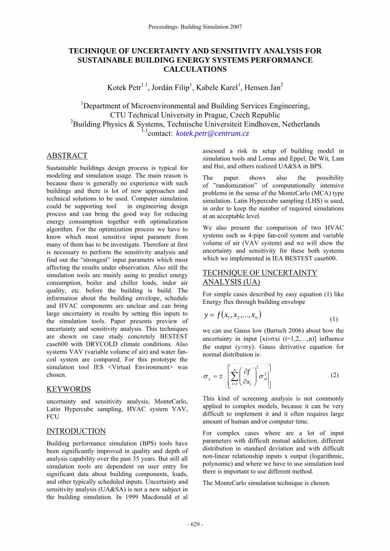
Figure 1 Diagrammatic analysis techniques of MCA

To analyze the uncertainty of building energy, given the uncertainty on the input parameters, MCA performs multiple evaluations with randomly selected model input parameters and involves the following steps:

To select ranges and distributions for each input parameter characterizing their uncertainty → generation of a sample for each input parameter from the selected distributions → evaluation of the model for each element of the sample → uncertainty analysis.

The pure MonteCarlo simulation cannot be applied for time-consuming problems, as it requires a large number of simulations. A small number of simulations can be used for the acceptable accuracy of statistical characteristics of response using the stratified sampling technique LHS (McKey, Conover 1979)

The LHS strategy has been used by many authors in different fields of engineering and with both simple and very complicated computational model (Novák et al. 1998).

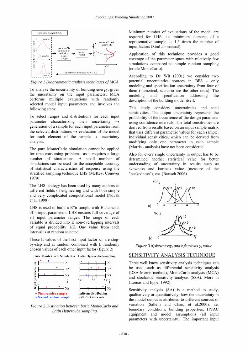
LHS is used to build a E*n sample with E elements of n input parameters. LHS ensures full coverage of all input parameter ranges. The range of each variable is divided into E non-overlapping intervals of equal probability 1/E. One value from each interval is at random selected.

These E values of the first input factor x1 are step-by-step and at random combined with E randomly chosen values of each other input factor (figure 2)

Figure 2 Distinction between basic MonteCarlo and

Latin Hypercube sampling

Minimum number of evaluations of the model are required for LHS, i.e. minimum elements of a representative sample, is 1,5 times the number of input factors (SimLab manual).

Application of this technique provides a good coverage of the parameter space with relatively few simulations compared to simple random sampling (crude MonteCarlo).

According to De Wit (2001) we consider two potential uncertainties sources in BPS - only modeling and specification uncertainty from four of them (numerical, scenario are the other ones). The modeling and specification addressing the description of the building model itself.

This study considers uncertainties and total sensitivities. The output uncertainty represents the probability of the occurrence of the design parameter using confidence intervals. The total sensitivities are derived from results based on an input sample matrix that uses different parametric values for each sample. Individual sensitivities, which can be derived from modifying only one parameter in each sample (Morris - analysis) have not been considered.

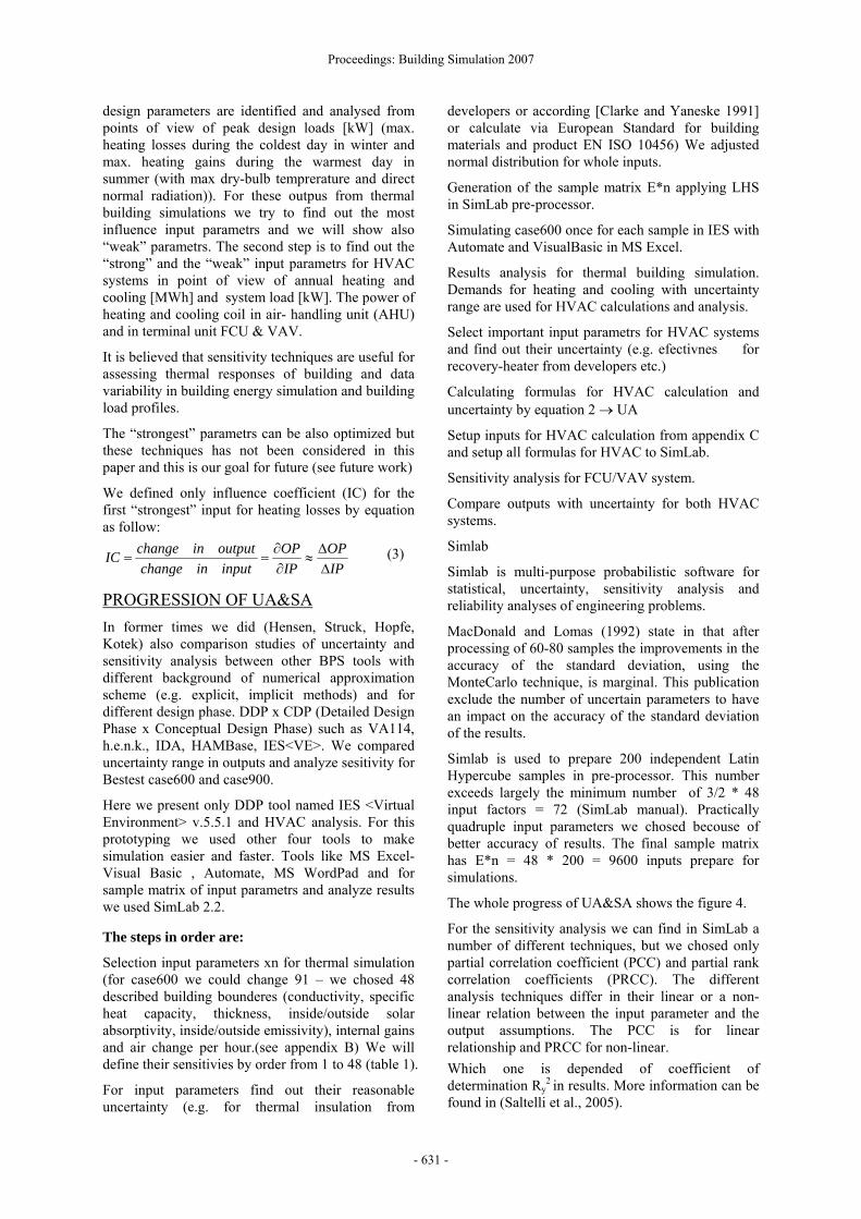
Also for every single uncertainty in output has to be determined another statistical value for better understading of uncertainty in results such as skewness and kurtosis value (measure of the "peakedness"), etc. (Bartsch 2006)

a)

b)

Figure 3 a)skewnessγ1 and b)kurtosis γ2 value

SENSITIVITY ANALYSIS TECHNIQUE Three well know sensitivity analysis techniques can be used such as differential sensitivity analysis (DSA-Morris method), MonteCarlo analysis (MCA) and stochastic sensitivity analysis (SSA). More in (Lomas and Eppel 1992).

Sensitivity analysis (SA) is a method to study, qualitatively or quantitatively, how the uncertainty in the model output is attributed to different sources of variation (Saltelli and Chan, et al.2000), i.e. boundary conditions, building properties, HVAC equipment and model assumptions (all input parameters with uncertainty). The important input

Proceedings: Building Simulation 2007

- 631 -

design parameters are identified and analysed from points of view of peak design loads [kW] (max. heating losses during the coldest day in winter and max. heating gains during the warmest day in summer (with max dry-bulb temprerature and direct normal radiation)). For these outpus from thermal building simulations we try to find out the most influence input parametrs and we will show also “weak” parametrs. The second step is to find out the “strong” and the “weak” input parametrs for HVAC systems in point of view of annual heating and cooling [MWh] and system load [kW]. The power of heating and cooling coil in air- handling unit (AHU) and in terminal unit FCU & VAV.

It is believed that sensitivity techniques are useful for assessing thermal responses of building and data variability in building energy simulation and building load profiles.

The “strongest” parametrs can be also optimized but these techniques has not been considered in this paper and this is our goal for future (see future work)

We defined only influence coefficient (IC) for the first “strongest” input for heating losses by equation as follow:

IPOP

IPOP

inputinchangeoutputinchangeIC

ΔΔ

≈∂∂

== (3)

PROGRESSION OF UA&SA In former times we did (Hensen, Struck, Hopfe, Kotek) also comparison studies of uncertainty and sensitivity analysis between other BPS tools with different background of numerical approximation scheme (e.g. explicit, implicit methods) and for different design phase. DDP x CDP (Detailed Design Phase x Conceptual Design Phase) such as VA114, h.e.n.k., IDA, HAMBase, IES<VE>. We compared uncertainty range in outputs and analyze sesitivity for Bestest case600 and case900.

Here we present only DDP tool named IES <Virtual Environment> v.5.5.1 and HVAC analysis. For this prototyping we used other four tools to make simulation easier and faster. Tools like MS Excel-Visual Basic , Automate, MS WordPad and for sample matrix of input parametrs and analyze results we used SimLab 2.2.

The steps in order are:

Selection input parameters xn for thermal simulation (for case600 we could change 91 – we chosed 48 described building bounderes (conductivity, specific heat capacity, thickness, inside/outside solar absorptivity, inside/outside emissivity), internal gains and air change per hour.(see appendix B) We will define their sensitivies by order from 1 to 48 (table 1).

For input parameters find out their reasonable uncertainty (e.g. for thermal insulation from

developers or according [Clarke and Yaneske 1991] or calculate via European Standard for building materials and product EN ISO 10456) We adjusted normal distribution for whole inputs.

Generation of the sample matrix E*n applying LHS in SimLab pre-processor.

Simulating case600 once for each sample in IES with Automate and VisualBasic in MS Excel.

Results analysis for thermal building simulation. Demands for heating and cooling with uncertainty range are used for HVAC calculations and analysis.

Select important input parametrs for HVAC systems and find out their uncertainty (e.g. efectivnes 　 for recovery-heater from developers etc.)

Calculating formulas for HVAC calculation and uncertainty by equation 2 → UA

Setup inputs for HVAC calculation from appendix C and setup all formulas for HVAC to SimLab.

Sensitivity analysis for FCU/VAV system.

Compare outputs with uncertainty for both HVAC systems.

Simlab

Simlab is multi-purpose probabilistic software for statistical, uncertainty, sensitivity analysis and reliability analyses of engineering problems.

MacDonald and Lomas (1992) state in that after processing of 60-80 samples the improvements in the accuracy of the standard deviation, using the MonteCarlo technique, is marginal. This publication exclude the number of uncertain parameters to have an impact on the accuracy of the standard deviation of the results.

Simlab is used to prepare 200 independent Latin Hypercube samples in pre-processor. This number exceeds largely the minimum number of 3/2 * 48 input factors = 72 (SimLab manual). Practically quadruple input parameters we chosed becouse of better accuracy of results. The final sample matrix has E*n = 48 * 200 = 9600 inputs prepare for simulations.

The whole progress of UA&SA shows the figure 4.

For the sensitivity analysis we can find in SimLab a number of different techniques, but we chosed only partial correlation coefficient (PCC) and partial rank correlation coefficients (PRCC). The different analysis techniques differ in their linear or a non-linear relation between the input parameter and the output assumptions. The PCC is for linear relationship and PRCC for non-linear. Which one is depended of coefficient of determination Ry

2 in results. More information can be found in (Saltelli et al., 2005).

Proceedings: Building Simulation 2007

- 632 -

Figure 4 Progress of uncertainty and sesitivity

analyses for thermal building model

CASE STUDIE - IEA BESTEST The Bestest procedure allows an inter-software performance evaluation for a many of predefined cases by defining performance limit. The building model for this paper was chosen:

CASE600 (Light weight construction) cca 90 kg/m2

Figure 5 Geometry of IEA bestest case

For this prototype we used IES <VE> which incorporates ApacheSim, a dynamic thermal simulation tool based on first-principles mathematical modeling of building heat transfer processes. It has been tested using ASHREA Standard 140 and qualifies as a Dynamic Model in the CIBSE system of model classification. (Crawley and Hand 2005). For the materials properties and other inputs with their uncertainty see appendix B.

We present here demand of heating losses and heating gains in extremes days and analyze uncertainty for these curves (figure 10,11). These demands are one of the inputs for HVAC calculation from the other ones. (see appendix C and figure 6,7 with marked input and output parameters).

In other words for the extreme days we calculate power for boiler and chiller and calculate UA&SA for them. Also for the whole year we calculated

annual heating and cooling and compared results for judged systems.

HVAC

For this prototype we decided to put some people and assumed, that case600 is a small single office.

We put inside 4 people (occupancy density 0,1 pers./m2) and ventilalation rates for no smoking people Ve,occ=10 l/s.occupant = 36m3/h.occ according to the CEN-CR 1752 with uncertainty 5 m3/h because some litterature or legislative say another little bit different value. Other potential sources of uncertainty in input parameters (figure 6,7) are extract in appendix C. The whole philosophy of both HVAC calculation is based on ASHREA: Fundamentals and ASHREA: Systems and Equipment what we presented in past (Kabele and Kotek 2006).

Uncertainties are calculated via function 2 and sensitiveness by setting equations from ASHREA-Fundamentals Chapter 5,6 for heating, cooling mass transfer, recuperation, mixing, etc to SimLab and analyze the results by post-processor.

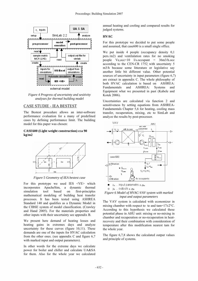
Figure 6 Model of HVAC-VAV system with marked

input and output parameters The VAV system is calculated with economizer in mixing chamber with respect to te and tam=17±2°C. According to this hypothesis we calculated these potential phase in AHU unit: mixing or no-mixing in chamber and recuperation or no-recuperation in heat-recovery and their combination with consideration of temperature after this modification nearest tam for the whole year.

The figure 6,7,8 shows the calculated output values and principle of systems.

Proceedings: Building Simulation 2007

- 633 -

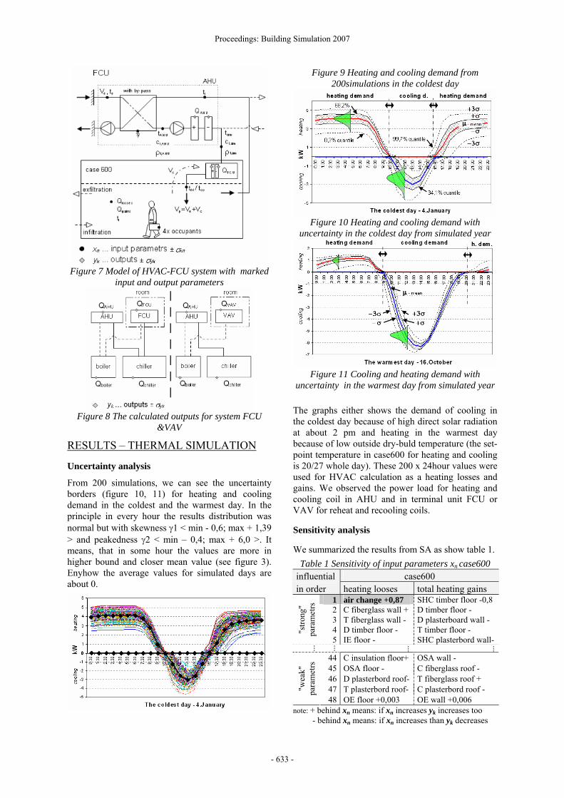
Figure 7 Model of HVAC-FCU system with marked

input and output parameters

Figure 8 The calculated outputs for system FCU

&VAV

RESULTS – THERMAL SIMULATION

Uncertainty analysis

From 200 simulations, we can see the uncertainty borders (figure 10, 11) for heating and cooling demand in the coldest and the warmest day. In the principle in every hour the results distribution was normal but with skewness γ1 < min - 0,6; max + 1,39 > and peakedness γ2 < min – 0,4; max + 6,0 >. It means, that in some hour the values are more in higher bound and closer mean value (see figure 3). Enyhow the average values for simulated days are about 0.

Figure 9 Heating and cooling demand from 200simulations in the coldest day

Figure 10 Heating and cooling demand with

uncertainty in the coldest day from simulated year

Figure 11 Cooling and heating demand with

uncertainty in the warmest day from simulated year The graphs either shows the demand of cooling in the coldest day because of high direct solar radiation at about 2 pm and heating in the warmest day because of low outside dry-buld temperature (the set-point temperature in case600 for heating and cooling is 20/27 whole day). These 200 x 24hour values were used for HVAC calculation as a heating losses and gains. We observed the power load for heating and cooling coil in AHU and in terminal unit FCU or VAV for reheat and recooling coils.

Sensitivity analysis

We summarized the results from SA as show table 1. Table 1 Sensitivity of input parameters xn case600

influential case600 in order heating looses total heating gains

1 air change +0,87 SHC timber floor -0,82 C fiberglass wall + D timber floor - 3 T fiberglass wall - D plasterboard wall - 4 D timber floor - T timber floor - "s

trong

" pa

ram

etrs

5 IE floor - SHC plasterbord wall-

...

...

...

...

44 C insulation floor+ OSA wall - 45 OSA floor - C fiberglass roof - 46 D plasterbord roof- T fiberglass roof + 47 T plasterbord roof- C plasterbord roof - "w

eak"

pa

ram

etrs

48 OE floor +0,003 OE wall +0,006 note: + behind xn means: if xn increases yk increases too - behind xn means: if xn increases than yk decreases

Proceedings: Building Simulation 2007

- 634 -

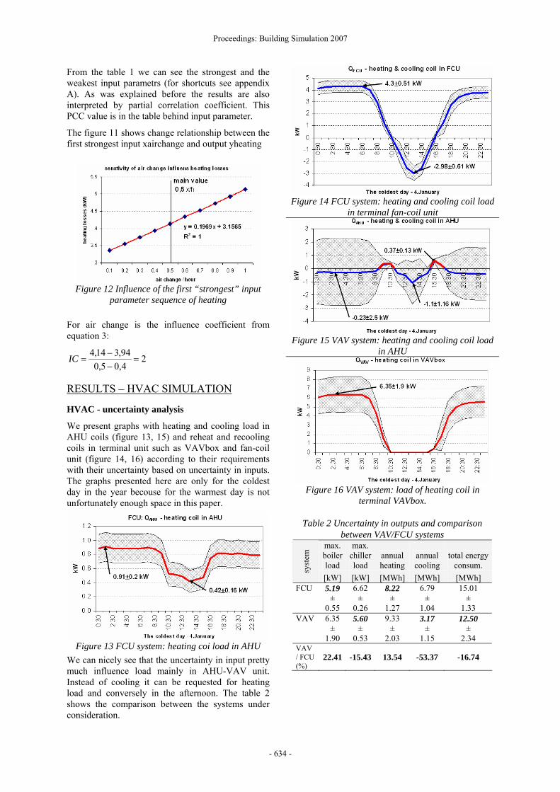
From the table 1 we can see the strongest and the weakest input parametrs (for shortcuts see appendix A). As was explained before the results are also interpreted by partial correlation coefficient. This PCC value is in the table behind input parameter.

The figure 11 shows change relationship between the first strongest input xairchange and output yheating

Figure 12 Influence of the first “strongest” input

parameter sequence of heating

For air change is the influence coefficient from equation 3:

24,05,094,314,4

=−−

=IC

RESULTS – HVAC SIMULATION

HVAC - uncertainty analysis

We present graphs with heating and cooling load in AHU coils (figure 13, 15) and reheat and recooling coils in terminal unit such as VAVbox and fan-coil unit (figure 14, 16) according to their requirements with their uncertainty based on uncertainty in inputs. The graphs presented here are only for the coldest day in the year becouse for the warmest day is not unfortunately enough space in this paper.

Figure 13 FCU system: heating coi load in AHU

We can nicely see that the uncertainty in input pretty much influence load mainly in AHU-VAV unit. Instead of cooling it can be requested for heating load and conversely in the afternoon. The table 2 shows the comparison between the systems under consideration.

Figure 14 FCU system: heating and cooling coil load in terminal fan-coil unit

Figure 15 VAV system: heating and cooling coil load in AHU

Figure 16 VAV system: load of heating coil in

terminal VAVbox.

Table 2 Uncertainty in outputs and comparison between VAV/FCU systems

max.boiler load

max.chiller load

annual heating

annual cooling

total energy consum. sy

stem

[kW] [kW] [MWh] [MWh] [MWh] FCU 5.19 6.62 8.22 6.79 15.01 ± ± ± ± ± 0.55 0.26 1.27 1.04 1.33 VAV 6.35 5.60 9.33 3.17 12.50 ± ± ± ± ± 1.90 0.53 2.03 1.15 2.34 VAV / FCU (%)

22.41 -15.43 13.54 -53.37 -16.74

Proceedings: Building Simulation 2007

- 635 -

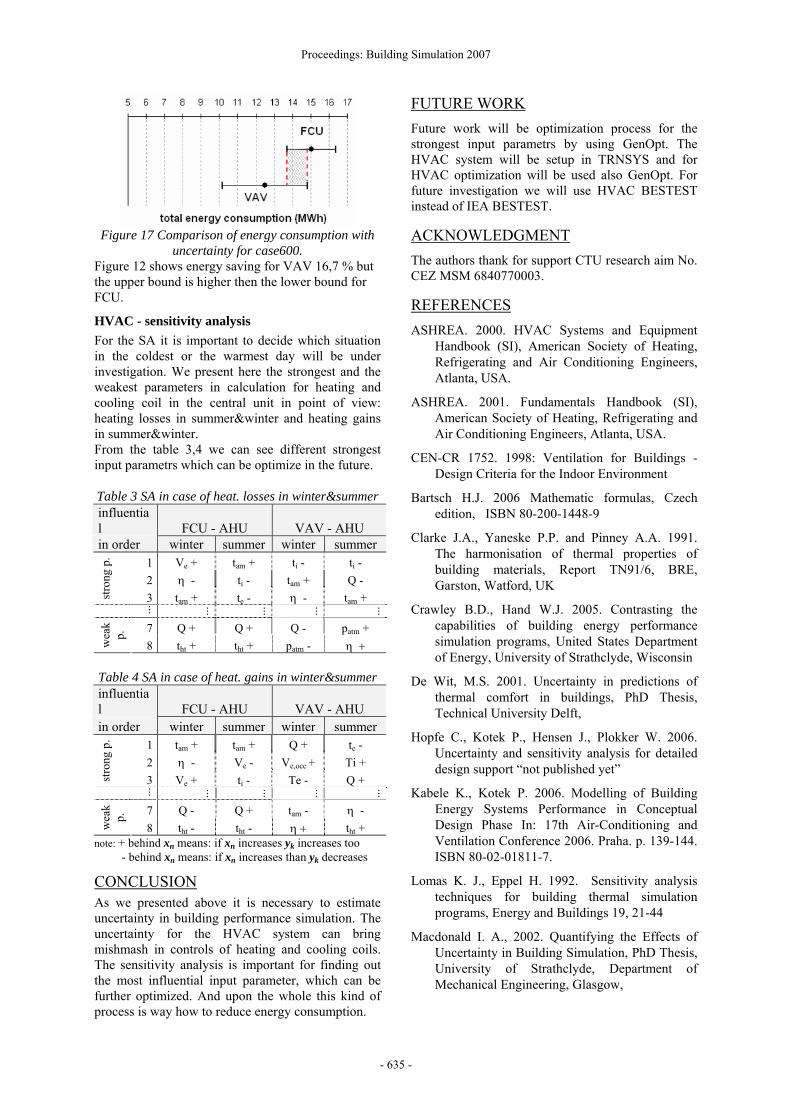
Figure 17 Comparison of energy consumption with

uncertainty for case600. Figure 12 shows energy saving for VAV 16,7 % but the upper bound is higher then the lower bound for FCU.

HVAC - sensitivity analysis For the SA it is important to decide which situation in the coldest or the warmest day will be under investigation. We present here the strongest and the weakest parameters in calculation for heating and cooling coil in the central unit in point of view: heating losses in summer&winter and heating gains in summer&winter. From the table 3,4 we can see different strongest input parametrs which can be optimize in the future. Table 3 SA in case of heat. losses in winter&summer influential FCU - AHU VAV - AHU in order winter summer winter summer

1 Ve + tam + ti - ti - 2 η - ti - tam + Q -

stro

ng p

.

3 tam + te - η - tam + ...

...

...

...

...

7 Q + Q + Q - patm +

wea

k p.

8 tht + tht + patm - η + Table 4 SA in case of heat. gains in winter&summer influential FCU - AHU VAV - AHU in order winter summer winter summer

1 tam + tam + Q + te - 2 η - Ve - Ve,occ + Ti +

stro

ng p

.

3 Ve + ti - Te - Q + ...

...

...

...

...

7 Q - Q + tam - η -

wea

k p.

8 tht - tht - η + tht + note: + behind xn means: if xn increases yk increases too - behind xn means: if xn increases than yk decreases

CONCLUSION As we presented above it is necessary to estimate uncertainty in building performance simulation. The uncertainty for the HVAC system can bring mishmash in controls of heating and cooling coils. The sensitivity analysis is important for finding out the most influential input parameter, which can be further optimized. And upon the whole this kind of process is way how to reduce energy consumption.

FUTURE WORK Future work will be optimization process for the strongest input parametrs by using GenOpt. The HVAC system will be setup in TRNSYS and for HVAC optimization will be used also GenOpt. For future investigation we will use HVAC BESTEST instead of IEA BESTEST.

ACKNOWLEDGMENT The authors thank for support CTU research aim No. CEZ MSM 6840770003.

REFERENCES ASHREA. 2000. HVAC Systems and Equipment

Handbook (SI), American Society of Heating, Refrigerating and Air Conditioning Engineers, Atlanta, USA.

ASHREA. 2001. Fundamentals Handbook (SI), American Society of Heating, Refrigerating and Air Conditioning Engineers, Atlanta, USA.

CEN-CR 1752. 1998: Ventilation for Buildings - Design Criteria for the Indoor Environment

Bartsch H.J. 2006 Mathematic formulas, Czech edition, ISBN 80-200-1448-9

Clarke J.A., Yaneske P.P. and Pinney A.A. 1991. The harmonisation of thermal properties of building materials, Report TN91/6, BRE, Garston, Watford, UK

Crawley B.D., Hand W.J. 2005. Contrasting the capabilities of building energy performance simulation programs, United States Department of Energy, University of Strathclyde, Wisconsin

De Wit, M.S. 2001. Uncertainty in predictions of thermal comfort in buildings, PhD Thesis, Technical University Delft,

Hopfe C., Kotek P., Hensen J., Plokker W. 2006. Uncertainty and sensitivity analysis for detailed design support “not published yet”

Kabele K., Kotek P. 2006. Modelling of Building Energy Systems Performance in Conceptual Design Phase In: 17th Air-Conditioning and Ventilation Conference 2006. Praha. p. 139-144. ISBN 80-02-01811-7.

Lomas K. J., Eppel H. 1992. Sensitivity analysis techniques for building thermal simulation programs, Energy and Buildings 19, 21-44

Macdonald I. A., 2002. Quantifying the Effects of Uncertainty in Building Simulation, PhD Thesis, University of Strathclyde, Department of Mechanical Engineering, Glasgow,

Proceedings: Building Simulation 2007

- 636 -

McKay M.D., Conover W.J. and Beckman R.J. 1979. A Comparison of Three Methods for Selecting Values of Input Variables in the Analysis of Output from a Computer Code. Technometrics Vol. 21: 239-245.

Novák D., Teplý B. and Keršner Z. 1998. The role of Latin Hypercube sampling method in reliability engineering. ICOSSAR-97; Proceedings 1998, Kyoto, Japan 1997: 403-409.

Saltelli A., Chan K., Scott E.M. 2000. Sensitivity Analysis, John Wiley and Sons, Chichester, UK,

Saltelli A., Tarantola S., Campolongo F., Ratto M., 2005. Sensitivity analysis in practice- a guide to assessing scientific models, Wiley

SIMLAB Version 2.2. 2004. Simulation Environment for uncertainty and sensitivity analysis, developed by the Joint Research Centre of the European commission. http://simlab.jrc.cec.eu.int

Struck C., Kotek P., Hensen J. 2006. On incorporating uncertainty analysis in abstract building performance simulation tools “not published yet”

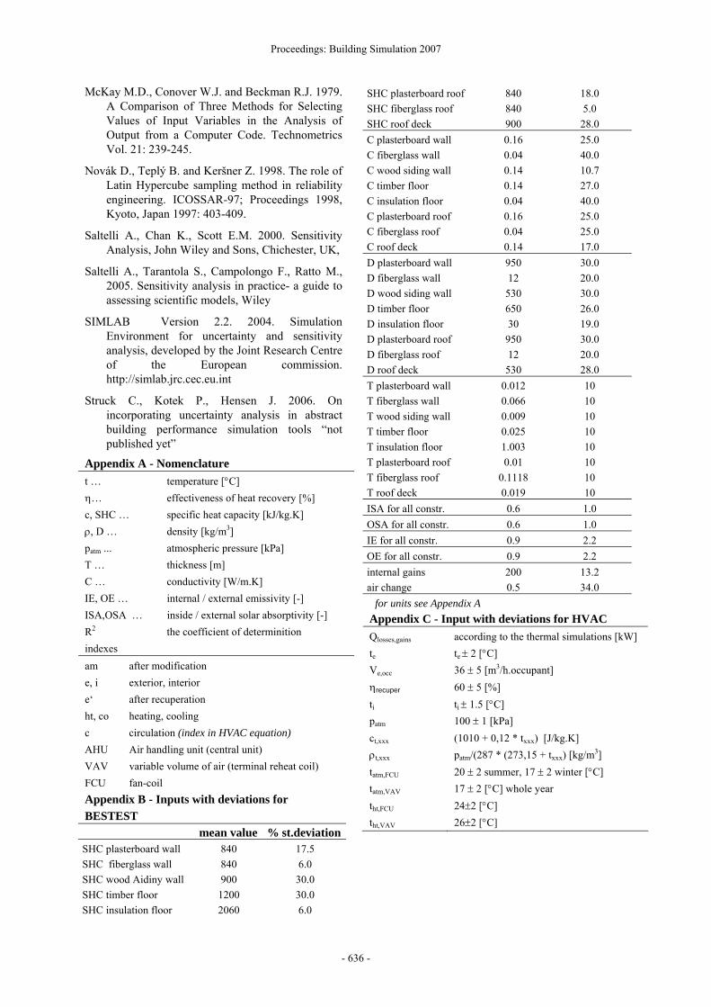
Appendix A - Nomenclature t … temperature [°C] η… effectiveness of heat recovery [%] c, SHC … specific heat capacity [kJ/kg.K] ρ, D … density [kg/m3] patm ... atmospheric pressure [kPa] T … thickness [m] C … conductivity [W/m.K] IE, OE … internal / external emissivity [-] ISA,OSA … inside / external solar absorptivity [-] R2 the coefficient of determinition indexes am after modification e, i exterior, interior e‘ after recuperation ht, co heating, cooling c circulation (index in HVAC equation) AHU Air handling unit (central unit) VAV variable volume of air (terminal reheat coil) FCU fan-coil Appendix B - Inputs with deviations for BESTEST mean value % st.deviationSHC plasterboard wall 840 17.5 SHC fiberglass wall 840 6.0 SHC wood Aidiny wall 900 30.0 SHC timber floor 1200 30.0 SHC insulation floor 2060 6.0

SHC plasterboard roof 840 18.0 SHC fiberglass roof 840 5.0 SHC roof deck 900 28.0 C plasterboard wall 0.16 25.0 C fiberglass wall 0.04 40.0 C wood siding wall 0.14 10.7 C timber floor 0.14 27.0 C insulation floor 0.04 40.0 C plasterboard roof 0.16 25.0 C fiberglass roof 0.04 25.0 C roof deck 0.14 17.0 D plasterboard wall 950 30.0 D fiberglass wall 12 20.0 D wood siding wall 530 30.0 D timber floor 650 26.0 D insulation floor 30 19.0 D plasterboard roof 950 30.0 D fiberglass roof 12 20.0 D roof deck 530 28.0 T plasterboard wall 0.012 10 T fiberglass wall 0.066 10 T wood siding wall 0.009 10 T timber floor 0.025 10 T insulation floor 1.003 10 T plasterboard roof 0.01 10 T fiberglass roof 0.1118 10 T roof deck 0.019 10 ISA for all constr. 0.6 1.0 OSA for all constr. 0.6 1.0 IE for all constr. 0.9 2.2 OE for all constr. 0.9 2.2 internal gains 200 13.2 air change 0.5 34.0 for units see Appendix A Appendix C - Input with deviations for HVAC Qlosses,gains according to the thermal simulations [kW] te te ± 2 [°C] Ve,occ 36 ± 5 [m3/h.occupant] ηrecuper 60 ± 5 [%] ti ti ± 1.5 [°C] patm 100 ± 1 [kPa] ct,xxx (1010 + 0,12 * txxx) [J/kg.K] ρt,xxx patm/(287 * (273,15 + txxx) [kg/m3] tatm,FCU 20 ± 2 summer, 17 ± 2 winter [°C] tatm,VAV 17 ± 2 [°C] whole year tht,FCU 24±2 [°C] tht,VAV 26±2 [°C]