TECHNIQUES IN COMBINATORICS { LECTURE NOTES Introduction · 2014-10-20 · TECHNIQUES IN COMBINATORICS { LECTURE NOTES W. T. GOWERS 1. Introduction The aim of this course is to equip

TECHNIQUES IN COMBINATORICS – LECTURE NOTES

W. T. GOWERS

1. Introduction

The aim of this course is to equip you with a set of tools that will help you solve certain

combinatorial problems much more easily than you would be able to if you did not have

these tools. So, as the title of the course suggests, the emphasis will be much more on the

methods used to prove theorems than on the theorems themselves: my main reason for

showing you proofs of theorems is to draw attention to and illustrate the methods.

I do not normally write lecture notes, but am prompted to do so by the fact that some

people at the first lecture were unable to take notes because there was not enough space

to sit down. I have not decided whether I will write notes for the whole course, but I’ll

make what I write available soon after writing it. One effect of this will be that the the

notes may well come to an abrupt end while I’m in the middle of discussing something.

2. The average lies between the minimum and the maximum

One of the simplest tools to describe – though it sometimes requires some ingenuity to

use – is the principle that a random variable cannot always be less than its mean and

cannot always be greater than its mean. More symbolically,

inf X < EX < supX.

By and large, we will be dealing with finite sample spaces, so the inf and sup are a min

and a max.

Perhaps the most famous example of a proof that uses this principle is Erdos’s lower

bound for the Ramsey number R(k, k).

Theorem 2.1. Let k, n ∈ N be such that k ≥ 2 and n ≤ 2(k−1)/2. Then there exists a

graph with n vertices that contains no clique or independent set of size k.

Proof. Let the edges of G be chosen randomly. That is, each edge is chosen with probability

1/2 and all choices are independent.1

2 W. T. GOWERS

For any k vertices x1, . . . , xk, the probability that they span a clique or independent

set is 2.2−(k2). Therefore, the expected number of cliques or independent sets of size k is

2(nk

)2−(k

2). (Note that we have just used linearity of expectation – the fact that this does

not require the random variables in question to be independent is often extremely helpful.)

By the basic principle above, there must exist a choice of edges such that the number of

cliques or independent sets of size k is at most 2(nk

)2−(k

2), so if we can ensure that this is

less than 1, then we will be done.

But(nk

)< nk/2, so 2

(nk

)2−(k

2) < nk2−k(k−1)/2. Therefore, if n ≤ 2(k−1)/2 we are done, as

claimed. �

The basic ideas of the proof above could be summarized as follows.

(1) Choose the graph randomly.

(2) Calculate the expected number of cliques/independent sets.

(3) Adjust n until the expected number falls below 1.

It is very important to learn to think of proofs in this sort of condensed way, trusting that

you can do the necessary calculations.

Here is a second example – also a theorem of Erdos. Call a set of integers sum free if it

contains no three elements a, b, c with a+ b = c.

Theorem 2.2. Let X be a set of n positive integers. Then X has a sum-free subset Y of

size at least n/3.

Before I give the proof, let me try to guess how Erdos thought of it. He might have

begun by thinking about ways of ensuring that sets are sum free. Perhaps he started with

the simple observation that the set of all odd numbers is sum free. Unfortunately, that

doesn’t help much because X might consist solely of even numbers. But we could try other

moduli.

What would the basic strategy be? What we’d like to do is find a large collection of

pretty dense sum-free sets that is in some sense evenly distributed, so that we can argue

that X must have a large intersection with one of them, and therefore have a large sum-free

subset. If we think about unions of residue classes mod p we soon spot that the interval

[p/3, 2p/3] is sum free, and having spotted that we realize that any non-zero multiple of

that interval (mod p) will have the same property. That gives us a collection of sets of

density 1/3 and each non-multiple of p is contained in the same number of sets (which is

what I meant by “in some sense evenly distributed”). That’s basically the proof, but here

are the details, expressed slightly differently.

TECHNIQUES IN COMBINATORICS – LECTURE NOTES 3

Proof. Let p > maxX and let a be chosen randomly from {1, 2, . . . , p− 1}. Let [p/3, 2p/3]

denote the set of integers mod p that lie in the real interval [p/3, 2p/3]. Thus, if p is of

the form 3m + 1, then [p/3, 2p/3] = {m + 1, . . . , 2m} and if p is of the form 3m + 2 then

[p/3, 2p/3] = {m+ 1, . . . , 2m+ 1}.In both cases, [p/3, 2p/3] contains at least a third of the non-zero residues mod p. There-

fore, for each x ∈ X, the probability that ax ∈ [p/3, 2p/3] is at least 1/3, so the expected

number of x ∈ X such that ax ∈ [p/3, 2p/3] is at least |X|/3.

Applying the basic principle, there must exist a such that for at least a third of the

elements x of X we have ax ∈ [p/3, 2p/3]. Let Y be the set of all such x. Then |Y | ≥ n/3.

But also Y is sum free, since if x, y, z ∈ Y and x+y = z, then we would have ax+ay ≡ az

mod p, which is impossible because the set [p/3, 2p/3] is sum free mod p. �

The difference between the way I presented the proof there and the way I described it in

advance is that in the proof above I kept the interval [p/3, 2p/3] fixed and multiplied X by

a random a mod p, whereas in the description before it I kept X fixed and took multiples

of the interval [p/3, 2p/3]. Thus, the two ideas are not different in any fundamental way.

Here is a summary of the above proof. Again, this is what you should remember rather

than the proof itself.

(1) The “middle third” of the integers mod p form a sum-free set mod p.

(2) If we multiply everything in X by some number and reduce mod p, then we preserve

all relationships of the form x+ y = z.

(3) But if p > maxX and we choose a randomly from non-zero integers mod p, then

on average a third of the elements of X end up in the middle third.

(4) Therefore, we are done, by the basic averaging principle.

The third example is a beautiful proof of a result about crossing numbers. The crossing

number of a graph G is the smallest possible number of pairs of edges that cross in any

drawing of G in the plane. We would like a lower bound for this number in terms of the

number of vertices and edges of G.

We begin with a well-known lemma that tells us when we are forced to have one crossing.

Lemma 2.3. Let G be a graph with n vertices and more than 3n − 6 edges. Then G is

not planar. (In other words, for every drawing of G in the plane there must be at least one

pair of edges that cross.)

4 W. T. GOWERS

Proof. Euler’s famous formula for drawings of planar graphs is that V −E+F = 2, where

V is the number of vertices, E the number of edges and F the number of faces (including

an external face that lies outside the entire graph).

Since each edge lies in two faces and each face has at least three edges on its boundary,

we must have (by counting pairs (e, f) where e is an edge on the boundary of face f) that

2E ≥ 3F , so that F ≤ 2E/3. It follows that V − E/3 ≥ 2, so E ≤ 3V − 6.

Therefore, if a graph with n vertices has more than 3n− 6 edges, then it is not planar,

as claimed. �

A famously non-planar graph is K5, the complete graph with five vertices. That has(52

)= 10 edges, and since 10 = 3× 5− 5, its non-planarity follows from the lemma above.

To avoid cumbersome sentences, I’m going to use the word “crossing” to mean “pair of

edges that cross” rather than “point where two edges cross”.

Corollary 2.4. Let G be a graph with n vertices and m edges. Then the number of

crossings is at least m− 3n.

Proof. Informally, we just keep removing edges that are involved in crossings until we get

down to 3n edges. More formally, the result is true when m = 3n + 1, by the previous

lemma. But if it is true for 3n + k, then for any graph with 3n + k + 1 edges there is at

least one edge that crosses another. Removing such an edge results in a graph with 3n+ k

edges and hence, by the inductive hypothesis, at least k crossings, which do not involve

the removed edge. So the number of crossings is at least k + 1 and we are done. �

That didn’t have much to do with averaging, but the averaging comes in at the next

stage.

The proof of the corollary above feels a bit wasteful, because each time we remove an

edge, we take account of only one crossing that involves that edge, when there could in

principle be many. We shall now try to “boost” the result to obtain a much better bound

when m is large.

Why might we expect that to be possible? The basic idea behind the next proof is

that if G has lots of edges and we choose a random induced subgraph of G, then it will

still have enough edges to force a crossing. The reason this helps is that (i) the random

induced subgraphs “cover G evenly” in the sense discussed earlier, and (ii) if we choose p

appropriately, then the previous corollary gives an efficient bound. So, roughly speaking,

we pass to a subgraph where the argument we have above is not wasteful, and then use the


evenness of the covering to argue that G must have had lots of crossings for the random

induced subgraph to have as many as it does.

Those remarks may seem a little cryptic: I recommend trying to understand them in

conjunction with reading the formal proof.

For a graph G I’ll use the notation v(G) for the number of vertices and e(G) for the

number of edges.

Theorem 2.5. Let G be a graph with n vertices and m ≥ 4n edges. Then G the crossing

number of G is at least m3/64n2.

Proof. Suppose we have a drawing of G with k crossings. We now choose a random induced

subgraph H of G by selecting the vertices independently with probability p = 4n/m. (The

reason for this choice of p will become clear later in the proof. For now we shall just call

it p. Note that once the vertices of H are specified, so are the edges, since it is an induced

subgraph.)

Then the expectation of v(H) is pn, since each vertex survives with probability p, the

expectation of e(H) is p2m, since each edge survives with probability p2, and the expecta-

tion of the number of crossings of H (in this particular drawing) is p4k, since each crossing

survives with probability k.

But we also know that the expected number of crossings is at least E(e(H) − 3v(H)),

by the previous corollary. We have chosen p such that e(H) − 3v(H) = p2m − 3pn =

4pn − 3pn = pn. Therefore, p4k ≥ pn, which implies that k ≥ p−3n = m3/64n2, as

stated. �

It might be worth explaining why we chose p to be 4n/m rather than, say, 3n/m. One

reason is that if you do the calculations with 3n/m, you get only six crossings in H (if

you are slightly more careful with the corollary) instead of pn crossings, and therefore the

answer you get out at the end is 6p−4, which is proportional to m4/n4. Except when m is

proportional to n2 (i.e., as big as it can be), this gives a strictly weaker bound.

But that is a slightly unsatisfactory answer, since it doesn’t explain why the bound is

weaker. The best reason I can come up with (but I think it could probably be improved)

is that Corollary 2.4 does not start to become wasteful until m is superlinear in n, since if

m is a multiple of n, then one normally expects an edge to be involved in only a bounded

number of crossings. Since increasing p from 3m/n to 4m/n doesn’t cost us much – it just

changes an absolute constant – we might as well give ourselves a number of edges that

grows linearly with v(H) rather than remaining bounded.

6 W. T. GOWERS

I think my summary of this proof would simply be, “Pick a random induced subgraph

with p just large enough for Corollary 2.4 to give a linear number of crossings, and use

averaging.”

The next result is another one where the basic idea is to find a family of sets that

uniformly covers the structure we are interested in, and then use an averaging argument to

allow ourselves to drop down to a member of that family. It is a famous result of Erdos, Ko

and Rado. Given a set X and a positive integer k, write X(k) for the set of all subsets of

X of size k. And given a family of sets A, say that it is intersecting if A∩B 6= ∅ whenever

A,B ∈ A.

Theorem 2.6. Let X be a set of size n, let k be such that 2k ≤ n, and let A ⊂ X(k) be

an intersecting family. Then |A| ≤(n−1k−1

).

Note that it is easy to see that this result is sharp, since we can take all sets of size k that

contain one particular element. Also, the condition that 2k ≤ n is obviously necessary,

since otherwise we can take the entire set X(k).

Proof. The following very nice proof is due to Katona. Let X = {x1, . . . , xk}, and define an

interval to be a set of the form {xj, xj+1, . . . , xj+k−1}, where addition of the indices is mod

n. There are n intervals, and if you want to form an intersecting family out of them, you

can pick at most k. To prove this, let {xj, . . . , xj+k−1} be one of the intervals in the family

and observe that for any other interval J in the family there must exist 1 ≤ h ≤ k−1 such

that exactly one of xj+h−1 and xj+h belongs to J , and for any h there can be at most one

such interval J .

The rest of the proof, if you are used to the basic method, is now obvious. We understand

families of intervals, so would like to cover X(k) evenly with them and see what we can

deduce from the fact that A cannot have too large an intersection with any one of them.

The obvious way of making this idea work is to choose a random ordering {x1, . . . , xn}of the elements of X and take the intervals with respect to that ordering. The expected

number of elements of A amongst these intervals is n|A|/(nk

), since each set in A has a

n/(nk

)chance of being an interval in this ordering (because there are n of them and

(nk

)sets

of size k, and by symmetry each set of size k has an equal probability of being an interval

in the ordering).

By the basic principle, there must therefore be an ordering such that at least n|A|/(nk

)sets in A are intervals. Since we also know that at most k intervals can all intersect each

other, we must have that n|A|/(nk

)≤ k, so |A| ≤ k

n

(nk

)=(n−1k−1

). �


If you like thinking about semi-philosophical questions, then you could try to find a good

explanation for why this argument gives the best possible bound.

Here is how I would remember the above proof.

(1) It is not too hard to show that amongst all the intervals of length k in a cyclic

ordering of the elements of X, at most k can intersect.

(2) Hence, by averaging over all cyclic orderings, the density of A in X(k) is at most

k/n.

Actually, that “it is not too hard to show” is slightly dishonest: I find that each time I

come back to this theorem I have forgotten the argument that proves this “obvious” fact.

But it is certainly a short argument and easy to understand.

For a final example, we shall give a proof of Sperner’s theorem, which concerns the

maximum possible size of an antichain: a collection of sets none of which is a proper

subset of another.

Theorem 2.7. Let X be a set of size n and let A be an antichain of subsets of X. Then

|A| ≤(

nbn/2c

).

Proof. Again we shall cover the structure we are interested in – the set of all subsets of X

– with a family of sets. An interesting twist here is that the covering is not even. But as

we shall see, this does not matter. In fact, it allows us to prove a stronger result than the

one stated.

The preliminary observation that gets the proof going is that for any collection of sets

of the form ∅, {x1}, {x1, x2}, . . . , {x1, x2, . . . , xn}, at most one of them can belong to A. So

our family will consist of sets of this kind, which are known as maximal chains.

Now we just do the obvious thing. Choose a random ordering x1, . . . , xn of the elements

of X and form the maximal chain ∅, {x1}, {x1, x2}, . . . , {x1, x2, . . . , xn}. If A ∈ A, then the

probability that it belongs to this chain is the probability that it equals the set {x1, . . . , xk},where k = |A|. This probability is

(nk

)−1. Therefore, the expected number of sets in A

that belong to the random maximal chain is∑

A∈A(

n|A|

)−1.

But it is also at most 1, since no maximal chain contains more than one set from A.

Since(

n|A|

)≤(

nbn/2c

)regardless of the size of A, it follows that |A| ≤

(nbn/2c

), as stated. �

I didn’t explicitly use the basic principle there, but I could have. I could have said that

by the principle there exists a maximal chain that contains at least∑

A∈A(

n|A|

)−1sets from

A. Then I would have concluded the proof from the fact that it also contains at most one

set from A.

8 W. T. GOWERS

This proof is another one with a very simple summary: pick a random maximal chain,

calculate the expected number of sets in A that it contains, and draw the obvious conclu-

sion.

I said that the proof gives a stronger result. What I meant by that can be stated as

follows. Suppose we assign a measure of(nk

)−1to each set of size k. Then the total measure

of A is, by the proof, at most 1. Since most sets have measure greater than(

nbn/2c

)−1, and

some have measure much greater than this, the result with this non-uniform measure is

significantly stronger.

3. Using mean and variance

So far we have seen that the inequality

inf X ≤ EX ≤ supX

is surprisingly useful. Now let’s do the same for a well-known identity that is not quite as

trivial, but is still very easy – so much so that it is again rather extraordinary how many

applications it has. This time I’ll give a proof.

Lemma 3.1. Let X be a random variable. Then varX = EX2 − (EX)2.

Proof. The variance varX is defined to be E(X − EX)2. But

E(X − EX)2 = EX2 − 2(EX)EX + (EX)2 = EX2 − (EX)2,

which gives us the identity. �

While we’re at it, here are a couple of useful inequalities. The first is Markov’s inequality.

Lemma 3.2. Let X be a random variable that takes non-negative real values. Then for

any non-negative real number, P[X ≥ a] ≤ a−1EX.

Proof. Let us bound the expectation from below by partitioning the sample space into the

set where X ≥ a and the set where X < a. Since X ≥ 0 on the second set, we get

EX ≥ aP[X ≥ a],

from which the inequality follows. �

The second is Chebyshev’s inequality.

Lemma 3.3. Let X be a random variable and let a ≥ 0. Then P[|X−EX| ≥ a] ≤ a−2varX.


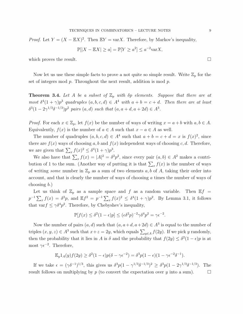
Proof. Let Y = (X − EX)2. Then EY = varX. Therefore, by Markov’s inequality,

P[|X − EX| ≥ a] = P[Y ≥ a2] ≤ a−2varX,

which proves the result. �

Now let us use these simple facts to prove a not quite so simple result. Write Zp for the

set of integers mod p. Throughout the next result, addition is mod p.

Theorem 3.4. Let A be a subset of Zp with δp elements. Suppose that there are at

most δ4(1 + γ)p3 quadruples (a, b, c, d) ∈ A4 with a + b = c + d. Then there are at least

δ3(1− 2γ1/3δ−1/3)p2 pairs (a, d) such that (a, a+ d, a+ 2d) ∈ A3.

Proof. For each x ∈ Zp, let f(x) be the number of ways of writing x = a+ b with a, b ∈ A.

Equivalently, f(x) is the number of a ∈ A such that x− a ∈ A as well.

The number of quadruples (a, b, c, d) ∈ A4 such that a + b = c + d = x is f(x)2, since

there are f(x) ways of choosing a, b and f(x) independent ways of choosing c, d. Therefore,

we are given that∑

x f(x)2 ≤ δ4(1 + γ)p3.

We also have that∑

x f(x) = |A|2 = δ2p2, since every pair (a, b) ∈ A2 makes a contri-

bution of 1 to the sum. (Another way of putting it is that∑

x f(x) is the number of ways

of writing some number in Zp as a sum of two elements a, b of A, taking their order into

account, and that is clearly the number of ways of choosing a times the number of ways of

choosing b.)

Let us think of Zp as a sample space and f as a random variable. Then Ef =

p−1∑

x f(x) = δ2p, and Ef 2 = p−1∑

x f(x)2 ≤ δ4(1 + γ)p2. By Lemma 3.1, it follows

that varf ≤ γδ4p2. Therefore, by Chebyshev’s inequality,

P[f(x) ≤ δ2(1− ε)p] ≤ (εδ2p)−2γδ4p2 = γε−2.

Now the number of pairs (a, d) such that (a, a+d, a+2d) ∈ A3 is equal to the number of

triples (x, y, z) ∈ A3 such that x+z = 2y, which equals∑

y∈A f(2y). If we pick y randomly,

then the probability that it lies in A is δ and the probability that f(2y) ≤ δ2(1− ε)p is at

most γε−2. Therefore,

Ey1A(y)f(2y) ≥ δ2(1− ε)p(δ − γε−2) = δ3p(1− ε)(1− γε−2δ−1).

If we take ε = (γδ−1)1/3, this gives us δ3p(1 − γ1/3δ−1/3)2 ≥ δ3p(1 − 2γ1/3δ−1/3). The

result follows on multiplying by p (to convert the expectation over y into a sum). �

10 W. T. GOWERS

It often happens in this area that one can do a slightly ugly argument using Markov’s

inequality or Chebyshev’s inequality, but with a bit more effort one can find a more elegant

argument that gives a better bound. Here we can do that by introducing the function

g(x) = f(x)− δ2p, which averages zero. We also know that∑

x g(x)2 ≤ γδ4p3, from which

it follows that∑

x∈A g(2x)2 ≤ γδ4p3, and therefore Ex∈Ag(2x)2 ≤ γδ3p2. Since the variance

of g is non-negative, it follows that (Ex∈Ag(2x))2 ≤ γδ3p2, so Ex∈Ag(2x) ≥ −γ1/2δ3/2p, and

therefore∑

x∈A g(2x) ≥ −γ1/2δ5/2p2.It follows that

∑x∈A f(2x) ≥ (δ3 − γ1/2δ5/2)p2 = δ3p2(1− γ1/2δ−1/2).

Once again I recommend not remembering the proof (or proofs) above, but a summary

such as this.

(1) The condition about the number of quadruples a+ b = c+ d can be interpreted as

an upper bound for the second moment of the function that tells you how many

ways you can write x as a+ b.

(2) The mean of this function is easy to determine, and it gives us that the variance is

small.

(3) But if the variance is small enough, then the function is close to its mean almost

everywhere, and in particular on most points of the form 2x for some x ∈ X.

We shall use second-moment methods quite a bit during this course. But to illustrate

that they can come up in a wide variety of contexts, we now give an application to analytic

number theory, namely a famous argument of Turan, which greatly simplified an earlier

proof of the same result that had been more number-theoretic in character.

We shall need the following estimate for the sum of the reciprocals of the primes up to

n. The proof will be left as an exercise (with hints) on an examples sheet. (It follows from

the prime number theorem, but can be proved much more easily.)

Lemma 3.5. There exists a positive integer C such that∑

p≤n p−1 ≤ log log n + C for

every n, where the sum is over primes p.

The theorem we shall now prove tells us that almost all numbers up to n have roughly

log log n prime factors.

Theorem 3.6. Let x be a randomly chosen integer between 1 and n. Let ν(x) be the

number of prime factors of x (without multiplicity). And let ω : N→ N be a function that

tends to infinity. Then

P[|ν(x)− log log n| > ω(n)√

log log n] = o(1).


Proof. To prove this, the rough idea is to show that the mean and variance of ν(x) are

both approximately log log n. Then the probability that |ν(x) − log log n| ≥ C√

log log n

will (if our approximation is good enough) be at most approximately C−2, by Chebyshev’s

inequality.

To estimate the mean and variance, we write ν(x) as a sum of random variables that

are easy to understand. For each prime p, let Xp be the random variable that takes the

value 1 if p|x and 0 otherwise. Then ν(x) =∑

pXp(x), where the sum is over all primes.

Let m = n1/2. The reason I wrote “the rough idea” above is that it turns out to be

convenient to estimate the mean and variance of ν1(x) =∑

p≤mXp(x) instead of those of ν.

Since x can have at most one prime factor greater than m, we have ν1(x) ≤ ν(x) ≤ ν1(x)+1

for every x. So the theorem for ν1 implies the theorem for ν.

The mean of Xp is n−1bn/pc, which lies between 1/p− 1/n and 1/p. Therefore,

(∑p≤m

1

p)− 1 ≤ Eν1 ≤

∑p≤m

1

p.

By Lemma 3.5, this is at most log log n+ C.

We want to work out the variance of ν1, so let us work out Eν21 and use Lemma 3.1. We

have

Eν21 = E(∑p≤m

Xp)2 =

∑p≤n

EXp +∑

p,q≤m, p6=q

EXpXq.

We also have

(Eν1)2 = (E∑p≤m

Xp)2 =

∑p≤m

(EXp)2 +

∑p,q≤m, p6=q

(EXp)(EXq).

It follows that

var ν1 ≤ log log n+ C +∑

p,q≤m, p6=q

(EXpXq − EXpEXq).

Let us now estimate EXpXq − EXpEXq, the covariance of Xp and Xq. It is at most

1

pq− (

1

p− 1

n)(

1

q− 1

n) ≤ 1

n(1

p+

1

q).

Adding these together for all p, q ≤ m gives us 2(m/n)∑

p≤n p−1, which is much smaller

than 1. Therefore, we find that varν1 ≤ log log n+ C + 1 and the theorem follows. �

A famous theorem of Erdos and Kac states that the distribution of ν(x) is roughly

normal with mean and variance log log n. Very roughly, the idea of the proof is to use

an argument like the one above to show that every moment of ν (or more precisely a

12 W. T. GOWERS

distribution where, as with ν1, one truncates the range of summation of the primes) is

roughly equal to the corresponding moment for the normal distribution, which is known

to imply that the distribution itself is roughly normal.

4. Using the Cauchy-Schwarz inequality

It is time to introduce some notation that has many virtues and has become standard

in additive combinatorics. If X is a set of size n and f is a function on X taking values in

R or C, then we write Ef or Exf(x) for n−1∑

x∈X f(x). For 1 ≤ p <∞ we define the Lp

norm of such a function f to be (Ex|f(x)|p)1/p, and write it as ‖f‖p. We also define the

L∞ norm ‖f‖∞ to be maxx |f(x)|.Typically, the Lp norm is useful when the function f is “flat”, in the sense that its values

mostly have the same order of magnitude. As we shall see later, we often like to set things

up so that we are considering functions where the values have typical order of magnitude 1.

However, sometimes we also encounter functions for which a few values have order of

magnitude 1, but most values are small. In this situation, it tends to be more convenient

to use the uniform counting measure on X rather than the uniform probability measure.

Accordingly, we define the `p norm of a function f defined on X to be (∑

x∈X |f(x)|p)1/p.We denote this by ‖f‖p as well, but if the meaning is unclear from the context, then we

can always write ‖f‖Lp and ‖f‖`p instead. Note that we also define the `∞ norm, but it is

equal to the L∞ norm. (That is because n1/p → 1 as p→∞, so the limit of the `p norms

equals the limit of the Lp norms.)

As with norms, we also define two inner products. Given two functions f, g : X → C,

these are given by the formulae Exf(x)g(x) and∑

x f(x)g(x). Both are denoted by 〈f, g〉,and again the context makes clear which is intended. We have the identity 〈f, f〉 = ‖f‖22,provided we either use expectations on both sides or sums on both sides.

Now let us have two lemmas. The first is the Cauchy-Schwarz inequality itself. Again,

the result has two interpretations, both of which are valid, provided one is consistent about

whether one is using sums or expectations.

Lemma 4.1. Let X be a finite set and let f and g be a function defined on X that takes

values in R or C. Then 〈f, g〉 ≤ ‖f‖2‖g‖2.

The sum version will be familiar to you already. If we use expectations instead, then

we have to divide the inner product by |X| and the square of each norm by |X|, so the

result still holds. The expectations version can also be thought of as an instance of the

probability version of the inequality, which states that for two random variables X and Y


we have EXY ≤ (E|X|2)1/2(E|Y |2)1/2. In this case, the random variables are obtained by

picking a random element of x and evaluating f and g. (Apologies for the overuse of the

letter X here.)

The second lemma is another surprisingly useful tool.

Lemma 4.2. Let X be a finite set and let f be a function from X to R or C. Then

|Exf(x)|2 ≤ Ex|f(x)|2.

Proof. If f is real valued, then Ex|f(x)|2 − |Exf(x)|2 is varf , by Lemma 3.1, and the

variance is non-negative by definition.

To prove the result in the complex case, we simply check that an appropriate general-

ization of Lemma 3.1 holds, which indeed it does, since

Ex|f(x)− Ef |2 = Ex

(|f(x)|2 − f(x)Ef − f(x)Ef + |Ef |2

)= Ex|f(x)|2 − |Ef |2.

This proves the lemma. �

A second proof is to apply the Cauchy-Schwarz inequality to the function f and the

constant function that takes the value 1 everywhere. That tells us that |Exf(x)| ≤ ‖f‖2,since the constant function has L2 norm 1, and squaring both sides gives the result. I myself

prefer the proof given above, because it is simpler, and because by focusing attention on

the variance it also makes another important fact very clear, which is that if |Exf(x)|2 is

almost as big as Ex|f(x)|2, then the variance of f is small, and therefore f is approximately

constant. (The “approximately” here means that the difference between f and a constant

function is small in the L2 norm.) This very simple principle is yet another one with legions

of applications. Indeed, we have already seen one: it was Theorem 3.4.

We have just encountered our first payoff for using expectations rather than sums. The

sums version of Lemma 4.2 is that |∑

x f(x)|2 ≤ |X|∑

x |f(x)|2. That is, we have to

introduce a normalizing factor |X| – the size of the set on which f takes its values. The

great advantage of the expectation notation is that for many arguments it allows one to

make all quantities one is interested in have order of magnitude 1, so we don’t need any

normalizing factors. This provides a very useful “checking of units” as our arguments

proceed.

Having stated these results, let us begin with a simple, but very typical, application.

Let us define a 4-cycle in a graph G to be an ordered quadruple (x, y, z, w) of vertices such

that all of xy, yz, zw, wx are edges. This is a non-standard definition because (i) we count

(x, y, z, w) as the same 4-cycle as, for instance, (z, y, x, w), and (ii) we do not insist that

14 W. T. GOWERS

x, y, z, w are distinct. However, the proofs run much more smoothly with this non-standard

definition, and from the results it is easy to deduce very similar results about 4-cycles as

they are usually defined.

Theorem 4.3. Let G be a graph with n vertices and αn2/2 edges. Then G contains at

least α4n4 4-cycles.

Proof. The average degree of G is αn. Therefore, by Lemma 4.2 the average square degree

is at least α2n2. So∑

x∈V (G) d(x)2 ≥ α2n3.

This sum is the number of triples (x, y, z) such that xy and xz are both edges. Let us

define the codegree d(y, z) to be the number of vertices x that are joined to both y and

z. Then the number of the triples (x, y, z) with xy, xz ∈ E(G) is equal to∑

y,z d(y, z).

Therefore, Ey,zd(y, z) ≥ α2n. By Lemma 4.2 again, Ey,zd(y, z)2 ≥ α4n2, so∑

y,z d(y, z)2 ≥α4n4.

But∑

y,z d(y, z)2 is the sum over all y, z of the number of pairs x, x′ such that yx, zx, yx′

and zx′ are all edges. In other words it is the number of 4-cycles (y, x, z, x′). �

It was slightly clumsy to pass from sums to expectations and back to sums again in

the above proof. But this clumsiness, rather than indicating that there is a problem with

expectation notation, actually indicates that we did not go far enough. We can get rid

of it by talking about the density of the graph, which is α, and proving that the 4-cycle

density (which I will define it later, but it should be clear what I am talking about) is at

least α4.

Our next application will use the full Cauchy-Schwarz inequality. As well as illustrating

an important basic technique, it will yield a result that will be important to us later on.

We begin by defining a norm on functions of two variables. We shall apply it to real-valued

functions, but we shall give the result for complex-valued functions, since they sometimes

come up in applications as well.

Let X and Y be finite sets and let f : X × Y → C. The 4-cycle norm ‖f‖� is defined

by the formula

‖f‖4 = Ex0,x1,y0,y1∈Xf(x0, y0)f(x0, y1)f(x1, y0)f(x1, y1).

The proof that this formula defines a norm is another application of the Cauchy-Schwarz

inequality and will be presented as an exercise on an examples sheet. Here we shall prove

an important inequality that tells us that functions with small 4-cycle norm have small

correlation with functions of rank 1. I shall include rather more chat in the proof than is


customary, since I want to convey not just the proof but the general method that can be

used to prove many similar results.

Theorem 4.4. Let X and Y be finite sets, let u : X → C, let v : Y → C and let

f : X → C. Then

|Ex,yf(x, y)u(x)v(y)| ≤ ‖f‖�‖u‖2‖v‖2.

Proof. With this sort of proof it is usually nicer to square both sides of the Cauchy-Schwarz

inequality, so let us look at the quantity |Ex,yf(x, y)u(x)v(y)|2.The basic technique, which is applied over and over again in additive combinatorics, is

to “pull out” a variable or variables, apply the Cauchy-Schwarz inequality, and expand out

any squared quantities. Here is the technique in action. We shall first pull out the variable

x, which means splitting the expectation into an expectation over x and an expectation

over y, with everything that depends just on x pulled outside the expectation over y. In

symbols,

Ex,yf(x, y)u(x)v(y) = Exu(x)Eyf(x, y)v(y).

Thus, the quantity we want to bound is |Exu(x)Eyf(x, y)v(y)|2.Note that Eyf(x, y)v(y) is a function of x. Therefore, by the (squared) Cauchy-Schwarz

inequality,

|Exu(x)Eyf(x, y)v(y)|2 ≤ ‖u‖22 Ex|Eyf(x, y)v(y)|2.

Now comes the third stage: expanding out the squared quantity. We have that

Ex|Eyf(x, y)v(y)|2 = ExEy0,y1f(x, y0)f(x, y1)v(y0)v(y1).

If you do not find that equality obvious, then you should introduce an intermediate step,

where the modulus squared is replaced by the product of the expectation over y with its

complex conjugate. But with a small amount of practice, these expansions become second

nature.

Now we shall repeat the whole process in order to find an upper bound for

|ExEy0,y1f(x, y0)f(x, y1)v(y0)v(y1)|.

Pulling out y0 and y1 gives

|ExEy0,y1f(x, y0)f(x, y1)v(y0)v(y1)| = |Ey0,y1v(y0)v(y1)Exf(x, y0)f(x, y1)|.

Then Cauchy-Schwarz gives

|Ey0,y1v(y0)v(y1)Exf(x, y0)f(x, y1)| ≤ (Ey0,y1|v(y0)v(y1)|2)(Ey0,y1|Exf(x, y0)f(x, y1)|2).

16 W. T. GOWERS

The first bracket on the right-hand side equals (Ey|v(y)|2)2 = ‖v‖42. Expanding the second

gives

Ey0,y1Ex0,x1f(x0, y0)f(x0, y1)f(x1, y0)f(x1, y1),

which equals ‖f‖4�.

Putting all this together gives us that

|Ex,yf(x, y)u(x)v(y)|4 ≤ ‖f‖4�‖u‖42‖v‖42,

which proves the result. �

5. A brief introduction to quasirandom graphs

A central concept in extremal combinatorics, and also in additive combinatorics, is that

of quasirandomness. We have already seen that randomly chosen objects have some nice

properties. In the late 1980s it was discovered that many of the properties exhibited by

random graphs are, in a loose sense, equivalent. That is, if you have a graph with one

“random-like” property, then it automatically has several other such properties. Graphs

with one, and hence all, of these properties came to be called quasirandom. A little later,

it was realized that the quasirandomness phenomenon (of several different randomness

properties being equivalent) applied to many other important combinatorial objects, and

also gave us an extremely useful conceptual tool for attacking combinatorial problems.

Perhaps the main reason quasirandomness is useful is the same as the reason that any

non-trivial equivalence is useful: we often want to apply one property, but a different,

equivalent, property is much easier to verify. I will discuss this in more detail when I have

actually presented some equivalences.

I would also like to draw attention to a device that I shall use in this section, which is

another very important part of the combinatorial armoury: analysing sets by looking at

their characteristic functions. Typically, one begins by wanting to prove a result about a

combinatorial object such as a bipartite graph, which can be thought of as a function from

a set X × Y to the set {0, 1}, and ends up proving a more general result about functions

from X × Y to the closed interval [0, 1], or even to the unit disc in C.

The characteristic function of a set A is often denoted by χA or 1A. My preference is

simply to denote it by A. That is, A(x) = 1 if x ∈ A and 0 otherwise, and similarly for

functions of more than one variable.


The next result is about functions, but it will soon be applied to prove facts about

graphs. We shall not need the complex version in this course, but we give it here since it

is only slightly harder than the real version.

Lemma 5.1. Let X and Y be finite sets, let f : X × Y → C, and let Ex,yf(x, y) = θ.

For each x, y, define g(x) to be Eyf(x, y) and f ′(x, y) to be f(x, y)− g(x), and for each x

define g′(x) to be g(x)− θ. Then

‖f‖4� ≥ ‖f ′‖4� + ‖g′‖42 + |θ|4.

Proof. Note first that

‖f‖4� = Ex,x′|Eyf(x, y)f(x′, y)|2

= Ex,x′|Ey(f′(x, y) + g(x))(f ′(x′, y) + g(x′))|2.

Since for each x we have Eyf′(x, y) = 0, this is equal to

Ex,x′|g(x)g(x′) + Eyf′(x, y)f ′(x′, y)|2.

When we expand the square, the off-diagonal term is

2<Ex,x′g(x)g(x′)Eyf ′(x, y)f ′(x′, y) = 2<Ey|Exg(x)f ′(x, y)|2 ≥ 0.

It follows that

‖f‖4� ≥ Ex,x′|g(x)|2|g(x′)|2 + Ex,x′|Eyf′(x, y)f ′(x′, y)|2 = ‖g‖42 + ‖f ′‖4�.

But ‖g‖22 = |θ|2 + ‖g′‖22, so ‖g‖42 ≥ |θ|4 + ‖g′‖42, so the result is proved. �

Given a bipartite graph G with finite vertex sets X and Y , define the density of G to

be e(G)/|X||Y | – that is, the number of edges in G divided by the number of edges in

the complete bipartite graph with vertex sets X and Y . Given that we want to focus on

quantities with order of magnitude 1, we shall prefer talking about densities of graphs to

talking about the number of edges they have.

For a similar reason, let us define the 4-cycle density of G to be the number of 4-cycles

in G divided by |X|2|Y |2. This is equal to

Ex,x′∈XEy,y′∈YG(x, y)G(x, y′)G(x′, y)G(x′, y′) = ‖G‖4�,

where I have used the letter G to denote the characteristic function of the graph G.

18 W. T. GOWERS

Corollary 5.2. Let X and Y be finite sets and let G be a bipartite graph with vertex sets

X and Y and density δ. Suppose that the 4-cycle density of G is at most δ4(1 + c4). Then

‖G− δ‖� ≤ 2cδ.

Proof. Applying Lemma 5.1 with f = G and θ = δ, we deduce that ‖f ′‖4� + ‖g′‖42 ≤ δ4c4,

where f ′(x, y) = G(x, y) − Ezf(x, z) and g′(x) = Ezf(x, z) − δ. This follows because the

4-cycle density assumption is equivalent to the statement that ‖G‖4� ≤ δ4(1 + c4).

If we regard g′ as a function of both x and y that happens not to depend on y, then we

find that

‖g′‖4� = Ex,x′g′(x)g′(x)g′(x′)g′(x′) = ‖g′‖42.

It follows that

‖G− δ‖� = ‖f ′ + g′‖� ≤ ‖f ′‖� + ‖g′‖� ≤ 2cδ,

as claimed. �

We now come to what is perhaps the most important (but certainly not the only im-

portant) fact about quasirandom graphs, which follows easily from what we have already

proved.

Given a bipartite graph G as above, and subsets A ⊂ X and B ⊂ Y , define the edge

weight η(A,B) to be the number of edges from A to B divided by |X||Y |. Although we

shall not need it immediately, it is worth also mentioning the edge density d(A,B), which

is the number of edges from A to B divided by |A||B|.

Theorem 5.3. Let X and Y be finite sets and let G be a bipartite graph with vertex sets

X and Y . Let the density of G be δ and suppose that the 4-cycle density of G is at most

δ4(1 + c4). Let A ⊂ X and B ⊂ Y be subsets of density α and β, respectively. Then

|η(A,B)− αβδ| ≤ 2cδ(αβ)1/2.

Proof. The edge weight η(A,B) is equal to Ex,yG(x, y)A(x)B(y). Therefore,

|η(A,B)− αβδ| = |Ex,y(G(x, y)− δ)A(x)B(y)|.

By Lemma 4.4, the right-hand side is at most ‖G− δ‖�‖A‖2‖B‖2. Corollary 5.2 gives us

that ‖G− δ‖� ≤ 2cδ, while ‖A‖2 and ‖B‖2 are equal to α1/2 and β1/2, respectively. This

proves the result. �

Now let us try to understand what the theorem above is saying. If you are not yet used

to densities rather than cardinalities, then you may prefer to reinterpret it in terms of the

latter. Then it is saying that the number of edges from A to B is, when c is small, close


to αβδ|X||Y | = δ|A||B|. Now if we had chosen our graph randomly with edge-probability

δ, then we would have expected the number of edges from A to B to be roughly δ|A||B|.So Theorem 5.3 is telling us that if a graph does not contain many 4-cycles (recall that

Theorem 4.3 states that the 4-cycle density must be at least δ4 and we are assuming that it

is not much more than that), then for any two sets A and B the number of edges between

A and B is roughly what you would expect. Let us say in this case that the graph has low

discrepancy.

An important remark here is that if we restate the result in terms of the density d(A,B)

then it says that |d(A,B) − δ| ≤ 2cδ(αβ)−1/2. Therefore, for fixed c the approximation

becomes steadily worse as the densities of A and B become smaller. This is a problem for

some applications, but often the sets A and B that we are interested in have a density that

is bounded below – that is, independent of the sizes of X and Y .

I like to think of Theorem 5.3 as a kind of local-to-global principle. We start with

a “local” condition – counting the number of 4-cycles – and deduce from it a “global”

principle – that the edges are spread about in such a way that there are approximately the

right number joining any two large sets A and B.

To explain that slightly differently, consider how one might try to verify the “global”

statement. If you try to verify it directly, you find yourself looking at exponentially many

pairs of sets (A,B), which is hopelessly inefficient. But it turns out that you can verify

it by counting 4-cycles, of which there are at most |X|2|Y |2, which is far smaller than

exponential. While this algorithmic consideration will not be our main concern, it is

another reflection of the fact that the implication is not just some trivial manipulation but

is actually telling us something interesting. And as it happens, there are contexts where

the algorithmic considerations are important too, though counting 4-cycles turns out not

to be the best algorithm for checking quasirandomness.

Before we go any further, let us prove an approximate converse to Theorem 5.3. For

simplicity, we shall prove it for regular graphs only and leave the general case as an exercise.

Theorem 5.4. Let X, Y and G be as in Theorem 5.3, let each vertex in X have degree

δ|Y |, let each vertex in Y have degree δ|X|, and suppose that the 4-cycle density of G is

at least δ4(1 + c). Then there exist sets A ⊂ X and B ⊂ Y of density α and β such that

η(A,B) ≥ αβδ(1 + c).

Proof. Our assumption about the 4-cycle density is that

Ex,x′∈X,y,y′∈YG(x, y)G(x, y′)G(x′, y)G(x′, y′) ≥ δ4(1 + c).

20 W. T. GOWERS

From this it follows that there exist vertices x′ ∈ X and y′ ∈ Y such that

Ex∈X,y∈YG(x, y)G(x, y′)G(x′, y) ≥ δ3(1 + c),

since if a random pair x′, y′ is chosen, the probability that G(x′, y′) is non-zero is δ. Let A

be the set of x such that G(x, y′) 6= 0 and let B be the set of y such that G(x′, y) 6= 0. In

other words, A and B are the neighbourhoods of y′ and x′, respectively. Then A and B

have density δ, by our regularity assumption, while

η(A,B) = Ex∈X,y∈YG(x, y)A(x)B(y) ≥ δ3(1 + c).

This proves the result. �

To adapt this argument to a proof for non-regular graphs, one first shows that unless

almost all degrees are approximately the same, there exist sets A and B for which η(A,B) is

significantly larger than αβδ. Then one shows that if almost all degrees are approximately

equal, then the argument above works, but with a small error introduced that slightly

weakens the final result.

In case it is not already clear, I call a bipartite graph of density δ quasirandom if its

4-cycle density is at most δ4(1 + c) for some small c, which is equivalent to saying that

η(A,B) is close to δαβ for all sets A ⊂ X and B ⊂ Y of density α and β, respectively.

If we want to talk about graphs, as opposed to bipartite graphs, we can simply take a

graph G with vertex set X, turn it into a bipartite graph by taking two copies of x and

joining x in one copy to y in the other if and only if xy is an edge of G, and use the

definitions and results from the bipartite case. In particular, the 4-cycle density of G is

simply |V (G)|−4 times the number of quadruples (x, y, z, w) such that xy, yz, zw and wx

are all edges of G, and G is quasirandom of density δ if the average degree is δ|V (G)| and

the 4-cycle density is δ4(1 + c) for some small c.

However, a slight difference between graphs and bipartite graphs is that we can talk

about the density of edges within a subset. That is, we define d(A) to be |A|−2 times the

number of pairs (x, y) ∈ A2 such that xy is an edge of G. We can also talk about the

weight η(A) of the edges in A, which I prefer to write analytically as

Ex,yA(x)A(y)G(x, y).

It is a straightforward exercise to prove that if η(A) is always close to δα2 (where α is

the density of A), then η(A,B) is always close to δαβ (where β is the density of B). The

converse is of course trivial.


In the exercises, you will also see that there is an equivalent formulation of quasirandom-

ness in terms of eigenvalues of the adjacency matrix of G. The natural matrix to associate

with a bipartite graph is not the adjacency matrix but the matrix G(x, y) where x ranges

over X and y ranges over Y . This matrix need not be symmetric, or even square, so we

don’t get an orthonormal basis of eigenvectors. Instead we need to use the singular value

decomposition. I do not plan to go into this in the course, though may perhaps set it as

an exercise.

One of the most striking facts about quasirandom graphs is that they contain the “right”

number of any small subgraph. I shall prove this for triangles in tripartite graphs and leave

the more general result as an exercise.

Given a graph G and two (not necessarily disjoint) sets A and B of its vertices, write

G(A,B) for the bipartite graph with vertex sets A and B where a ∈ A is joined to b ∈ Bif and only if ab is an edge of G.

Theorem 5.5. Let G be a tripartite graph with vertex sets X, Y, Z. Let the densities

of G(X, Y ), G(Y, Z) and G(X,Z) be α, β and γ, respectively. Suppose that the 4-cycle

densities of G(X, Y ), G(Y, Z) and G(X,Z) are at most α4(1+c4), β4(1+c4) and γ4(1+c4).

Then the triangle density differs from αβγ by at most 4c(αβγ)1/2.

Proof. The quantity we wish to estimate is

Ex,y,zG(x, y)G(y, z)G(x, z).

Let us write G(x, y) = f(x, y) + α, G(y, z) = g(y, z) + β and G(x, z) = h(x, z) + γ. Then

Ex.y.zG(x, y)G(y, z)G(x, z)− αβγ

can be expanded as

Ex,y,z(f(x, y)G(y, z)G(x, z) + αg(y, z)G(x, z) + αβh(x, z)).

By Corollary 5.2, ‖f‖� ≤ 2cα. Therefore, for each fixed z, we have

|Ex,yf(x, y)G(y, z)G(x, z)| ≤ 2cα(ExG(x, z))1/2(EyG(y, z))1/2,

22 W. T. GOWERS

by Theorem 4.4. Taking the expectation over z, we get that

||Ex,y,zf(x, y)G(y, z)G(x, z)| ≤ 2cαEz(ExG(x, z))1/2(EyG(y, z))1/2

≤ 2cα(EzExG(x, z))1/2(EzEyG(y, z))1/2

= 2cα(βγ)1/2,

where the second inequality was Cauchy-Schwarz.

Essentially the same argument shows that

|αEx.y.zg(y, z)G(x, z)| ≤ 2cαβγ1/2,

while the third term is zero. This gives us the bound stated (and in fact, a better bound,

but one that is uglier to state and not of obvious importance). �

I cannot stress strongly enough that it is the basic method of proof that matters above,

and not the precise details of its implementation. So let me highlight what I regard as the

basic method, and then indicate how it could have been implemented differently.

(1) A step that is useful all over additive combinatorics is to decompose a function F

that averages δ into two parts f + δ, so that we can deal with the constant function

δ, which we often regard as the main term, and the function f , which averages zero

and which in many contexts is a kind of “error”. (The word “error” is reasonable

only if the function is small in some sense. Here the sense in question is that of

having a small 4-cycle norm.)

(2) Having done that, one breaks up the original expression into terms, and attempts

to show that all terms that involve the error functions are small.

In the proof above, I chose a slightly non-obvious (but often quite useful) way of imple-

menting step 2. A more obvious way of doing it would simply have been to split the

expression

Ex,y,z(α + f(x, y)(β + g(y, z))(γ + h(x, z))

into eight terms. The main term would again be αβγ and the remaining seven terms (three

of which are zero) can be estimated using Theorem 4.4 as in the proof above.

A second remark I would like to make is that if we use the low-discrepancy property

of quasirandom graphs instead, we get an easy combinatorial argument that again shows

that the number of triangles is roughly as expected. Here is a quick sketch.


A preliminary observation, which we have already mentioned, is that if a graph has low

discrepancy, then almost all degrees are roughly the same. We now pick a random vertex

x ∈ X. Then with high probability its neighbourhoods in Y and Z have densities roughly α

and γ, respectively. When that happens, then by the low-discrepancy property in G(Y, Z),

the edge weight between these two neighbourhoods is approximately αβγ. This shows that

for almost all x ∈ X, the probability that a random triangle containing x belongs to the

graph is roughly αβγ, and from that the result follows.

Note that we did not use the low discrepancy of the graphs G(X, Y ) and G(X,Z) there,

but simply the fact that they are approximately regular. If you look at the proof of

Theorem 5.5 above, you will see that a similar remark applies: to bound the first term

we needed ‖f‖� to be small, but to bound the second, it would have been sufficient to

know that Eyg(y, z) was small for almost all z, which is the same as saying that for almost

all z the density of the neighbourhood of z in Y is roughly β|Y |. (One can therefore go

further – in both arguments – and say that what matters is a one-sided regularity. For

instance, in the discrepancy argument sketched above, we care about the densities of the

neighbourhoods in Y and Z of vertices in x, but we do not care about the densities in X

of the neighbourhoods of vertices in Y and Z.)

A third remark is that if we are dealing with a graph rather than a tripartite graph, we

can prove a similar result by making it tripartite in a similar way to the way we made it

bipartite earlier. That is, we take three copies of the vertex set and join vertices according

to whether the corresponding vertices are joined in the original graph.

As mentioned already, the above proofs work with obvious modifications to show that

quasirandom graphs contain the right number of copies of any fixed graph. I described the

result as striking: what is striking about it is that the converse implication is completely

trivial: if you have the right number of any fixed graph, then in particular you have the

right number of 4-cycles.

Finally, I should mention that there are close connections between the quasirandomness

of a graph and the sizes of the eigenvalues of its adjacency matrix. This is an important

topic, which will be covered (or at least introduced) in the examples sheets.

Documents

TECHNIQUES IN COMBINATORICS { LECTURE NOTES Introduction · 2014-10-20 · TECHNIQUES IN COMBINATORICS { LECTURE NOTES W. T. GOWERS 1. Introduction The aim of this course is to equip