Embed Size (px)
Citation preview
Technische Universitat Graz
Boundary integral formulations of eigenvalueproblems for elliptic differential operators with
singular interactions and their numericalapproximation by boundary element methods
M. Holzmann and G. Unger
Berichte aus demInstitut fur Angewandte Mathematik
Bericht 2019/5

Technische Universitat Graz
Boundary integral formulations of eigenvalueproblems for elliptic differential operators with
singular interactions and their numericalapproximation by boundary element methods
M. Holzmann and G. Unger
Berichte aus demInstitut fur Angewandte Mathematik
Bericht 2019/5

Technische Universitat GrazInstitut fur Angewandte MathematikSteyrergasse 30A 8010 Graz
WWW: http://www.applied.math.tugraz.at
c© Alle Rechte vorbehalten. Nachdruck nur mit Genehmigung des Autors.
BOUNDARY INTEGRAL FORMULATIONS OF EIGENVALUE
PROBLEMS FOR ELLIPTIC DIFFERENTIAL OPERATORS
WITH SINGULAR INTERACTIONS AND THEIR NUMERICAL
APPROXIMATION BY BOUNDARY ELEMENT METHODS
MARKUS HOLZMANN AND GERHARD UNGER
Abstract. In this paper the discrete eigenvalues of elliptic second order dif-
ferential operators in L2pRnq, n P N, with singular δ- and δ1-interactions are
studied. We show the self-adjointness of these operators and derive equivalentformulations for the eigenvalue problems involving boundary integral opera-
tors. These formulations are suitable for the numerical computations of thediscrete eigenvalues and the corresponding eigenfunctions by boundary element
methods. We provide convergence results and show numerical examples.
1. Introduction
Schrodinger operators with singular interactions supported on sets of measurezero play an important role in mathematical physics. The simplest example areSchrodinger operators with point interactions, which were already introduced in thebeginnings of quantum mechanics [27, 35]. The importance of these models comesfrom the fact that they reflect the physical reality still to a reasonable exactnessand that they are explicitly solvable. The point interactions are used as idealizedreplacements for regular potentials, which are strongly localized close to those pointssupporting the interactions, and the eigenvalues can be computed explicitly via analgebraic equation involving the values of the fundamental solution corresponding tothe unperturbed operator evaluated at the interaction support, cf. the monograph[1] and the references therein.
Inspired by this idea, Schrodinger operators with singular δ- and δ1-interactionssupported on hypersurfaces (i.e. manifolds of codimension one like curves in R2 orsurfaces in R3) where introduced. Such interactions are used as idealized replace-ments of regular potentials which are strongly localized in neighborhoods of thesehypersurfaces e.g. in the mathematical analysis of leaky quantum graphs, cf. thereview [15] and the references therein, and in the theory of photonic crystals [18].Note that in the case of δ-potentials this idealized replacement is rigorously justifiedby an approximation procedure [3]. The self-adjointness and qualitative spectralproperties of Schrodinger operators with δ- and δ1-interactions are well understood,see e.g. [6,7,11,15,16,29] and the references therein, and the discrete eigenvalues canbe characterized via an abstract version of the Birman Schwinger principle. How-ever, following the strategy from the point interaction model one arrives, instead of
Key words and phrases. elliptic differential operators, δ and δ1-interaction, discrete eigenvalues,integral operators, boundary element method.
1
arX
iv:1
907.
0428
2v1
[m
ath.
SP]
9 J
ul 2
019
2 M. HOLZMANN AND G. UNGER
an algebraic equation, at a boundary integral equation involving the fundamentalsolution for the unperturbed operator.
In this paper we suggest boundary element methods for the numerical approx-imations of these boundary integral equations. With this idea of computing theeigenvalues of the differential operators with singular interactions numerically, wegive a link of these models to the original explicitly solvable models with point in-teractions. As theoretical framework for the description of the eigenvalues in termsof boundary integral equations we use the theory of eigenvalue problems for holo-morphic and meromorphic Fredholm operator-valued functions [19,20,26]. For theapproximation of this kind of eigenvalue problems by the Galerkin method thereexists a complete convergence analysis in the case that the operator-valued functionis holomorphic [21,22,34]. This analysis provides error estimates for the eigenvaluesand eigenfunctions as well as results which guarantee that the approximation of theeigenvalue problems does not have so-called spurious eigenvalues, i. e., additionaleigenvalues which are not related to the original problem.
Other approaches for the numerical approximation of eigenvalues of differentialoperators with singular interactions are based on finite element methods, where Rnis replaced by a big ball, whose size can be estimated with the help of Agmon typeestimates. Moreover, in [12, 17, 30] it is shown in various settings in space dimen-sions n P t2, 3u that Schrodinger operators with δ-potentials supported on curves(for n “ 2) or surfaces (for n “ 3) can be approximated in the strong resolventsense by Hamiltonians with point interactions. An improvement of this approachis presented in [14]. This allows also to compute numerically the eigenvalues of thelimit operator.
Let us introduce our problem setting and give an overview of the main results.Consider a strongly elliptic and formally symmetric partial differential operator inRn, n P N, of the form
P :“ ´nÿ
j,k“1
BkajkBj `nÿ
j“1
`
ajBj ´ Bjaj˘
` a,
see Section 3 for details. Moreover, let Ωi be a bounded Lipschitz domain withboundary Σ :“ BΩi, let Ωe :“ RnzΩi, and let ν be the unit normal to Ωi. Eventually,let γ be the Dirichlet trace and Bν the conormal derivative at Σ (see (3.4) for thedefinition). We are interested in the eigenvalues of two kinds of perturbations of Pas self-adjoint operators in L2pRnq which are formally given by
Aα :“ P ` αδΣ and Bβ :“ P ` βxδ1Σ, ¨yδ1Σ,
where δΣ is the Dirac δ-distribution supported on Σ and the interaction strengthsα, β are real valued functions defined on Σ with α, β´1 P L8pΣq. For P “ ´∆ theseoperators have been intensively studied e.g. in [7, 11, 15, 16], for certain stronglyelliptic operators and smooth surfaces several properties of Aα and Bβ have beeninvestigated in [6,29]. For the realization of Aα as an operator in L2pRnq we remarkthat if the distribution Aαf is generated by an L2-function, then fi/e :“ f æ Ωi/e
has to fulfill
(1.1) γfi “ γfe and Bνfe ´ Bνfi “ αγf on Σ,
3
as then the singularities at Σ compensate, cf. [7]. In a similar manner, if thedistribution Bβf is generated by an L2-function, then f has to fulfill
(1.2) Bνfi “ Bνfe and γfe ´ γfi “ βBνf on Σ.
Hence, the relations (1.1) and (1.2) are necessary conditions for a function f tobelong to the domain of definition of Aα and Bβ , respectively. Our aims are toshow the self-adjointness of Aα and Bβ in L2pRnq and to fully characterize theirdiscrete spectra in terms of boundary integral operators. We pay particular atten-tion to establish formulations which fit in the framework of eigenvalue problems forholomorphic and meromorphic Fredholm operator-valued functions and which areaccessible for boundary element methods. This requires a thorough analysis of theinvolved boundary integral operators.
When using boundary element methods for the approximations of discrete eigen-values of Aα and Bβ it is convenient to consider the related transmission problems.A value λ belongs to the point spectrum of Aα if and only if there exists a nontrivialf P L2pRnq satisfying
pP ´ λqf “ 0 in RnzΣ,γfi “ γfe, on Σ,
Bνfe ´ Bνfi “ αγf on Σ.
(1.3)
Similarly, λ belongs to the point spectrum of Bβ if and only if there exists a non-trivial f P L2pRnq satisfying
pP ´ λqf “ 0 in RnzΣ,Bνfi “ Bνfe on Σ,
γfe ´ γfi “ βBνf on Σ.
(1.4)
This shows that the eigenvalue problems for Aα and Bβ are closely related totransmission problems for P ´λ, as they were treated in [24,25], and the strategiespresented there are useful for the numerical calculation of the eigenvalues of Aαand Bβ .
For the analysis of the spectra of Aα and Bβ a good understanding of the unper-turbed operator A0 being the self-adjoint realization of P with no jump conditionat Σ and some operators related to the fundamental solution of P´λ are necessary.Assume for λ P ρpA0q Y σdiscpA0q that Gpλ;x, yq is the integral kernel of a suitableparamatrix associated to P ´ λ which is explained in detail in Section 3; for λ inthe resolvent set ρpA0q it is in fact a fundamental solution for P ´ λ. We remarkthat the knowledge of Gpλ;x, yq or at least a good approximation of this function isessential for our numerical considerations. We introduce the single layer potentialSLpλq and the double layer potential DLpλq acting on sufficiently smooth functionsϕ : Σ Ñ C and x P RnzΣ as
SLpλqϕpxq :“
ż
Σ
Gpλ;x, yqϕpyqdσpyq
and
DLpλqϕpxq :“
ż
Σ
pBν,yGpλ;x, yqqϕpyqdσpyq.
As we will see, all solutions of pP ´ λqf “ 0 will be closely related to the ranges ofSLpλq and DLpλq. Moreover, the boundary integral operators which are formally
4 M. HOLZMANN AND G. UNGER
given by
Spλqϕ :“ γSLpλqϕ, T pλq1ϕ :“ BνpSLpλqϕqi ` BνpSLpλqϕqe,
and
T pλqϕ :“ γpDLpλqϕqi ` γpDLpλqϕqe, Rpλqϕ :“ ´BνDLpλqϕ,
will play an important role. While the properties of the above operators are well-known for many special cases, e.g. for P “ ´∆, the corresponding results are, tothe best of the authors’ knowledge, not easily accessible in the literature for generalP. Hence, for completeness we spend some efforts in Section 3.3 to provide thoseproperties of the above integral operators which are needed for our considerations.Eventually, following a strategy from [9], we show that the discrete eigenvaluesof A0 can be characterized as the poles of an operator-valued function which isbuilt up by the operators Spλq, T pλq, T pλq1, and Rpλq; see also [13] for relatedresults. Compared to [9] our formulation is particularly useful for the applicationof boundary element methods to compute the discrete eigenvalues of A0 numerically,as the appearing operators are easily accessible for numerical computations.
In order to introduce Aα and Bβ rigorously, consider the Sobolev spaces
H1PpΩq :“ tf P H1pΩq : Pf P L2pΩqu.
Inspired by (1.1) and (1.2) we define Aα as the partial differential operator inL2pRnq given by
Aαf :“ Pfi ‘ Pfe,
domAα :“
f “ fi ‘ fe P H1PpΩiq ‘H
1PpΩeq : γfi “ γfe, Bνfe ´ Bνfi “ αγf
(
,
(1.5)
and Bβ by
Bβf :“ Pfi ‘ Pfe,
domBβ :“
f “ fi ‘ fe P H1PpΩiq ‘H
1PpΩeq : Bνfi “ Bνfe, γfe ´ γfi “ βBνf
(
.
(1.6)
In Section 4 and 5 we show the self-adjointness of these operators in L2pRnq and viathe Weyl theorem that the essential spectra of Aα and Bβ coincide with the essentialspectrum of the unperturbed operator A0. Hence, to know the spectral profile ofAα and Bβ we have to understand the discrete eigenvalues of these operators. Thecharacterization of the discrete eigenvalues of Aα and Bβ in terms of boundaryintegral equations depends on the discrete spectrum of the unperturbed operatorA0 being empty or not. Let us consider the first case. It turns out that λ P ρpA0q
is a discrete eigenvalue of Aα if and only if there exists a nontrivial ϕ P L2pΣq suchthat
(1.7) pI ` αSpλqqϕ “ 0.
Similarly, the existence of a discrete eigenvalue λ P ρpA0q of Bβ is equivalent to the
existence of a corresponding nontrivial ψ P H12pΣq which satisfies
(1.8) pβ´1 `Rpλqqψ “ 0.
As shown in Sections 4 and 5 the boundary integral formulations in (1.7) and (1.8)are eigenvalue problems for holomorphic Fredholm operator-valued functions. Theseeigenvalue problems can be approximated by standard boundary element methods.
5
The convergence of the approximations follows from well-known abstract conver-gence results [21, 22, 34], which are summarized in Section 2. In the case thatσdiscpA0q is not empty, still all eigenvalues of Aα and Bβ in ρpA0q can be character-ized and computed using (1.7) and (1.8), respectively. For the possible eigenvaluesAα and Bβ which lie in σdiscpA0q also boundary integral formulations are providedwhich are accessible by boundary element methods and discussed in detail in Sec-tion 4 and 5.
Finally, let us note that our model also contains certain classes of magneticSchrodinger operators with singular interactions with rather strong limitations forthe magnetic field. Nevertheless, one could use our strategy and the Birman-Schwinger principle for magnetic Schrodinger operators with more general magneticfields provided in [4, 30] to compute the discrete eigenvalues of such Hamiltoniansnumerically. Also, an extension of our results to Dirac operators with δ-shell inter-actions [5] would be of interest, but this seems to be a rather challenging problem.
Let us shortly describe the structure of the paper. In Section 2 we recall somebasic facts on eigenvalue problems of holomorphic Fredholm operator-valued func-tions and on the approximation of this kind of eigenvalue problems by the Galerkinmethod. In Section 3 we introduce the elliptic differential operator P and the asso-ciated integral operators and investigate the properties of the unperturbed operatorA0. Sections 4 and 5 are devoted to the analysis of Aα and Bβ , respectively. Weintroduce these operators as partial differential operators in L2pRnq, show theirself-adjointness and derive boundary integral formulations to characterize their dis-crete eigenvalues. Moreover, we discuss how these boundary integral equations canbe solved numerically by boundary element methods, provide convergence results,and give some numerical examples.
Notations. Let X and Y be complex Hilbert spaces. The set of all anti-linearbounded functionals on X and Y are denoted by X˚ and Y ˚, respectively, and thesesquilinear duality product in X˚ ˆX, which is linear in the first and anti-linearin the second argument, is p¨, ¨q; the underlying spaces of the duality product willbe clear from the context. Next, the set of all bounded and everywhere definedlinear operators from X to Y is BpX,Y q; if X “ Y , then we simply write BpXq :“BpX,Xq. For A P BpX,Y q the adjoint A˚ P BpY ˚, X˚q is uniquely determined bythe relation pAx, yq “ px,A˚yq for all x P X and y P Y ˚.
If A is a self-adjoint operator in a Hilbert space, then its domain, range, andkernel are denoted by domA, ranA, and kerA. The resolvent set, spectrum, dis-crete, essential, and point spectrum are ρpAq, σpAq, σdiscpAq, σesspAq, and σppAq,respectively. Finally, if Λ is an open subset of C and A : Λ Ñ BpX,X˚q, then wesay that λ P Λ is an eigenvalue of Ap¨q, if kerApλq ‰ t0u.
Acknowledgements. We are specially grateful to O. Steinbach for encouragingus to work on this project. Moreover, we thank J. Behrndt and J. Rohleder forhelpful discussions and literature hints.
6 M. HOLZMANN AND G. UNGER
2. Galerkin approximation of eigenvalue problems for holomorphicFredholm operator-valued functions
In this section we present basic results of the theory of eigenvalue problemsfor holomorphic Fredholm operator-valued functions [19, 26] and summarize mainresults of the convergence analysis of the Galerkin approximation of such eigenvalueproblems [21, 22, 36]. These results build the abstract framework which we willutilize in order to show the convergence of the boundary element method for theapproximation of the discrete eigenvalues of Aα as well as of Bβ which lie in ρpA0q.Under specified conditions the convergence for discrete eigenvalues of Aα and Bβin σdiscpA0q is also guaranteed.
Let X be a Hilbert space and let Λ Ă C be an open and connected subsetof C. We consider an operator-valued function F : Λ Ñ BpX,X˚q which de-pends holomorphically on λ P Λ, i.e., for each λ0 P Λ the derivative F 1pλ0q :“limλÑλ0
1λ´λ0
Fpλq ´ Fpλ0qLpX,X˚q exists. Moreover, we assume that Fpλq is
a Fredholm operator of index zero for all λ P Λ and that it satisfies a so-calledGarding’s inequality, i. e., there exists a compact operator Cpλq : X Ñ X˚ and aconstant cpλq ą 0 for all λ P Λ such that
(2.1) | ppFpλq ` Cpλqqu, uq | ě cpλqu2X for all u P X.
We consider the nonlinear eigenvalue problem for the operator-valued func-tion Fp¨q of the form: find eigenvalues λ P Λ and corresponding eigenelementsu P Xzt0u such that
(2.2) Fpλqu “ 0.
In the following we assume that the set tλ P Λ : DFpλq´1 P BpX˚, Xqu is not empty.Then the set of eigenvalues in Λ has no accumulation points inside of Λ [19, Cor.XI 8.4]. The dimension of the null space kerFpλq of an eigenvalue λ is called thegeometric multiplicity of λ. An ordered collection of elements u0, u1, . . . , um´1 inX is called a Jordan chain of pλ, u0q, if it is an eigenpair and if
nÿ
j“0
1
j!F pjqpλqun´j “ 0 for all n “ 0, 1, . . . ,m´ 1
is satisfied, where F pjq denotes the jth derivative. The length of any Jordan chainof an eigenvalue is finite [26, Lem. A.8.3]. Elements of any Jordan chain of aneigenvalue λ are called generalized eigenelements of λ. The closed linear space ofall generalized eigenelements of an eigenvalue λ is called generalized eigenspace ofλ and is denoted by GpF , λq. The dimension of the generalized eigenspace GpF , λqis finite [26, Prop. A.8.4] and it is referred to as algebraic multiplicity of λ.
2.1. Galerkin approximation. For the approximation of the eigenvalue prob-lem (2.2) we consider a conforming Galerkin approximation. We assume thatpXN qNPN is a sequence of finite-dimensional subspaces of X such that the orthog-onal projection PN : X Ñ XN converges pointwise to the identity I : X Ñ X, i.e.,for all u P X we have
(2.3) PNu´ uX “ infvNPXN
vN ´ uX Ñ 0 as N Ñ8.
7
The Galerkin approximation of the eigenvalue problem reads as: find eigenpairspλN , uN q P ΛˆXNzt0u such that
(2.4) pFpλN quN , vN q “ 0 for all vn P XN .
For the formulation of the convergence results we need the definition of the gapδV pV1, V2q of two subspaces V1, V2 of a normed space V :
δV pV1, V2q :“ supv1PV1
v1V “1
infv2PV2
v1 ´ v2V .
Theorem 2.1. Let F : Λ Ñ BpX,X˚q be a holomorphic operator-valued functionand assume that for each λ P Λ there exist a compact operator Cpλq : X Ñ X˚
and a constant cpλq ą 0 such that inequality (2.1) is satisfied. Further, supposethat pXN qNPN is a sequence of finite-dimensional subspaces of X which fulfills theproperty (2.3). Then the following holds true:
(i) (Completeness of the spectrum of the Galerkin eigenvalue problem) For eacheigenvalue λ P Λ of the operator-valued function Fp¨q there exists a sequencepλN qN of eigenvalues of the Galerkin eigenvalue problem (2.4) such that
λN Ñ λ as N Ñ8.
(ii) (Non-pollution of the spectrum of the Galerkin eigenvalue problem) Let K Ă
Λ be a compact and connected set such that BK is a simple rectifiable curve.Suppose that there is no eigenvalue of Fp¨q in K. Then there exists anN0 P N such that for all N ě N0 the Galerkin eigenvalue problem (2.4) hasno eigenvalues in K.
(iii) Let D Ă Λ be a compact and connected set such that BD is a simple recti-
fiable curve. Suppose that λ P D is the only eigenvalue of F in D. Thenthere exist an N0 P N and a constant c ą 0 such that for all N ě N0 wehave:(a) For all eigenvalues λN of the Galerkin eigenvalue problem (2.4) in D
|λ´ λN | ď cδXpGpF , λq, XN q1`δXpGpF˚, λq, XN q
1`
holds, where F˚p¨q :“ pFp¨qq˚ is the adjoint function with respect tothe pairing p¨, ¨q for X˚ ˆX and ` is the maximal length of a Jordanchain corresponding to λ.
(b) If pλN , uN q is an eigenpair of (2.4) with λN P D and uN X “ 1, then
infuPkerpF,λq
u´ uN X ď c p|λN ´ λ| ` δXpkerpF , λq, XN qq .
Proof. The Galerkin method fulfills the required properties in order to apply theabstract convergence results in [21, 22, 36] to eigenvalue problems for holomorphicoperator-valued functions which satisfy inequality (2.1), see [34, Lem. 4.1]. We referto [21, Thm. 2] for assertion (i) and (ii), and to [22, Thm. 3] for (iii)a). The errorestimate in (iii)b) is a consequence of [36, Thm. 4.3.7].
3. Strongly elliptic differential operators and associated integraloperators
In this section we introduce the class of elliptic differential operators which willbe perturbed by the singular δ- and δ1-interactions supported on a hypersurface
8 M. HOLZMANN AND G. UNGER
Σ, and we introduce the integral operators Spλq, T pλq, T pλq1, and Rpλq in Sec-tion 3.3 in a mathematically rigorous way and recall their properties, which willbe of importance for our further studies. Eventually, in Section 3.4 we show howthe discrete eigenvalues of A0 can be characterized with the help of these boundaryintegral operators. But first, we introduce our notations for function spaces whichwe use in this paper.
3.1. Function spaces. For an open set Ω Ă Rn, n P N, and k P N0Yt8u we writeCkpΩq for the set of all k-times continuously differentiable functions and
C8b pΩq :“ tf P C8pΩq : f,∇f are boundedu.
Moreover, the Sobolev spaces of order s P R are denoted by HspΩq, see [28, Chap-ter 3] for their definition.
In the following we assume that Ω Ă Rn is a Lipschitz domain in the senseof [28, Definition 3.28]. We emphasize that Ω can be bounded or unbounded, butBΩ has to be compact. Note that in this case we can identify HspRnzBΩq withHspΩq ‘ HspRnzΩq. With the help of the integral on BΩ with respect to theHausdorff measure we get in a natural way the definition of L2pBΩq. In a similarflavor, we denote the Sobolev spaces on BΩ of order s P r0, 1s by HspBΩq, see [28]for details on their definition. For s P r´1, 0s we define HspBΩq :“ pH´spBΩqq˚ asthe anti-dual space of H´spBΩq.
Finally, we recall that the Dirichlet trace operator C8pΩq Q f ÞÑ f |BΩ can beextended for any s P p 1
2 ,32 q to a bounded and surjective operator
(3.1) γ : HspΩq Ñ Hs´12pBΩq;
cf. [28, Theorem 3.38].
3.2. Strongly elliptic differential operators. Let ajk, aj , a P C8b pRnq, n P N,
and j, k P t1, . . . , nu, and define the differential operator
(3.2) Pf :“ ´nÿ
j,k“1
BkpajkBjfq `nÿ
j“1
`
ajBjf ´ Bjpajfq˘
` af
in the sense of distributions. We assume that ajk “ akj and that a is real valued;then P is formally symmetric. Moreover, we assume that P is strongly elliptic, thatmeans there exists a constant C ą 0 independent of x such that
nÿ
j,k“1
ajkpxqξjξk ě C|ξ|2
holds for all x P Rn and all ξ P Cn.
Next, define for an open subset Ω Ă Rn the sesquilinear form ΦΩ : H1pΩqˆH1pΩqby
(3.3) ΦΩrf, gs :“
ż
Ω
«
nÿ
j,k“1
ajkBjfBkg `nÿ
j“1
`
ajpBjfqg ` fpajBjgq˘
` afg
ff
dx.
In the following assume that Ω Ă Rn is a Lipschitz set, let ν be the unit normalvector field at BΩ pointing outwards Ω, denote by γ the Dirichlet trace operator,
9
see (3.1), and introduce for f P H2pΩq the conormal derivative Bνf by
(3.4) Bνf :“nÿ
k“1
νk
nÿ
j“1
γpajkBjfq `nÿ
j“1
νjγpajfq.
Then one can show that
(3.5) pPf, gqL2pΩq “ ΦΩrf, gs ´ pBνf, γgqL2pBΩq, f P H2pΩq, g P H1pΩq,
holds. Next, we introduce the Sobolev space
(3.6) H1PpΩq :“
f P H1pΩq : Pf P L2pΩq(
,
where Pf is understood in the distributional sense. It is well known that theconormal derivative Bν has a bounded extension
(3.7) Bν : H1PpΩq Ñ H´12pBΩq,
such that (3.5) extends to
(3.8) pPf, gqL2pΩq “ ΦΩrf, gs ´ pBνf, γgq, f P H1PpΩq, g P H
1pΩq,
where the term on the boundary in (3.5) is replaced by the duality product inH´12pΣq and H12pΣq, see [28, Lemma 4.3]. We remark that this formula alsoholds for Ω “ Rn, then the term on the boundary is not present.
Our first goal is to construct the unperturbed self-adjoint operator A0 in L2pRnqassociated to P. With the help of [28, Theorem 4.7] it is not difficult to showthat the sesquilinear form ΦRn fulfills the assumptions of the first representationtheorem [23, Theorem VI 2.1], so we can define A0 as the self-adjoint operatorcorresponding to ΦRn . The following result is well-known, the simple proof is leftto the reader.
Lemma 3.1. Let P be given by (3.2) and let the form ΦRn be defined by (3.3).Then ΦRn is densely defined, symmetric, bounded from below, and closed. Theself-adjoint operator A0 in L2pRnq associated to ΦRn is
(3.9) A0f “ Pf, domA0 “ H2pRnq.
Assume that Ωi is a bounded Lipschitz domain in Rn with boundary Σ :“ BΩi,let ν be the unit normal to Ωi, and set Ωe :“ RnzΩi. Then it follows from [28,Theorem 4.20] that a function f “ fi ‘ fe P H
1PpΩiq ‘H
1PpΩeq fulfills
(3.10) f P domA0 “ H2pRnq ðñ γfi “ γfe and Bνfi “ Bνfe.
Next, we review some properties of the resolvent of A0 which are needed later.In the following, let λ P ρpA0q Y σdiscpA0q be fixed. Recall that a map G is called aparamatrix for P´λ in the sense of [28, Chapter 6], if there exist integral operatorsK1,K2 with C8-smooth integral kernels such that
GpP ´ λqu “ u´K1u and pP ´ λqGu “ u´K2u
holds for all u P E˚pRnq, where E˚pRnq is the set of all distributions with compactsupport, cf. [28]. A paramatrix is a fundamental solution for P ´ λ, if the aboveequation holds with K1 “ K2 “ 0.
Let us denote the orthogonal projection onto kerpA0 ´ λq by pPλ and set
(3.11) Pλ :“ I ´ pPλ.
10 M. HOLZMANN AND G. UNGER
Note that Pλ “ I for λ P ρpA0q and if te1, . . . eNu, N :“ dim kerpA0 ´ λq, is a basisof kerpA0 ´ λq for λ P σdiscpA0q, then
pPλf “Nÿ
k“1
pf, ekqL2pRnqek “
ż
Rn
Kp¨, yqfpyqdy, Kpx, yq :“Nÿ
k“1
ekpxqekpyq,
for all f P L2pRnq. We remark that the integral kernel K is a C8-function byelliptic regularity [28, Theorem 4.20]. By the spectral theorem we have that A0´λis boundedly invertible in PλpL
2pRnqq. Therefore, the map
(3.12) Gpλq :“ PλpA0 ´ λq´1Pλ
is bounded in L2pRnq, and it is a paramatrix for P ´ λ, as
(3.13) pP ´ λqPλpA0 ´ λq´1Pλf “ PλpA0 ´ λq
´1PλpP ´ λqf “ Pλf “ f ´ pPλf
holds for all f P C80 pRnq. Therefore, by [28, Theorem 6.3 and Corollary 6.5] thereexists an integral kernel Gpλ;x, yq such that for almost every x P Rn
(3.14) Gpλqfpxq “ż
Rn
Gpλ;x, yqfpyqdy, f P L2pRnq.
In the following proposition we show some additional mapping properties of Gpλqfor λ P ρpA0q Y σdiscpA0q; they are standard and well-known, but for completenesswe give the proof of this proposition.
Proposition 3.2. Let A0 be defined by (3.9), let λ P ρpA0qYσdiscpA0q, and let Gpλqbe given by (3.12). Then, for any s P r´2, 0s the mapping Gpλq can be extended toa bounded operator
(3.15) Gpλq : HspRnq Ñ Hs`2pRnq.
Moreover, the map
ρpA0q Q λ ÞÑ pA0 ´ λq´1
is holomorphic in BpHspRnq, Hs`2pRnqq.
Proof. Assume that λ P ρpA0q Y σdiscpA0q is fixed. First, we show that
(3.16) Gpλq : L2pRnq Ñ H2pRnq
is bounded. The operator in (3.16) is well-defined, as ranGpλq “ ranPλpA0 ´
λq´1Pλ “ Pλdom pA0 ´ λq Ă H2pRnq. Moreover, we claim that the operatorin (3.16) is closed, then it is also bounded by the closed graph theorem. Letpfnq Ă L2pRnq be a sequence and let f P L2pRnq and g P H2pRnq be such that
fn Ñ f in L2pRnq and Gpλqfn Ñ g in H2pRnq.
Since Gpλq is bounded in L2pRnq, we get Gpλqfn Ñ Gpλqf in L2pRnq. Moreover, asH2pRnq is continuously embedded in L2pRnq, we also have
Gpλqfn Ñ g in L2pRnq.
Hence, we conclude Gpλqf “ g, which shows that the operator in (3.16) is closedand thus, bounded.
Since the operator in (3.16) is bounded for any λ P ρpA0qYσdiscpA0q, we concludeby duality that also
Gpλq : H´2pRnq Ñ L2pRnq
11
is bounded. Therefore, interpolation yields that the mapping property (3.15) holdsalso for all s P p´2, 0q.
In order to show that λ ÞÑ pA0 ´ λq´1 is holomorphic in BpHspRnq, Hs`2pRnqq
for any s P r´2, 0s in a fixed point λ0 P ρpA0q, we note that the resolvent identityimplies
“
1´ pλ´ λ0qpA0 ´ λ0q´1
‰
pA0 ´ λq´1 “ pA0 ´ λ0q
´1.
If λ is close to λ0, we deduce from the Neumann formula that 1´pλ´λ0qpA0´λ0q´1
is boundedly invertible in Hs`2pRnq and hence,
pA0 ´ λq´1 “
“
1´ pλ´ λ0qpA0 ´ λ0q´1
‰´1pA0 ´ λ0q
´1.
In particular, pA0 ´ λq´1 is uniformly bounded in BpHspRnq, Hs`2pRnqq for λbelonging to a small neighborhood of λ0 and continuous in λ. Employing this andonce more the resolvent identity
pA0 ´ λq´1 ´ pA0 ´ λ0q
´1 “ pλ´ λ0qpA0 ´ λq´1pA0 ´ λ0q
´1,
we find that ρpA0q Q λ ÞÑ pA0 ´ λq´1 is holomorphic in BpHspRnq, Hs`2pRnqq.
3.3. Surface potentials associated to P. In this section we introduce severalfamilies of integral operators associated to the paramatrix Gpλq which will be ofimportance in the study of Aα and Bβ and for the numerical calculation of theireigenvalues. Remark that many of the properties shown below are well known forspecial realizations of P, for instance P “ ´∆, but for completeness we also providethe proofs for general P.
Throughout this section assume that Σ is the boundary of a bounded Lipschitzdomain Ωi, set Ωe :“ RnzΩi, and let ν be the unit normal to Ωi. If f is a functiondefined on Rn, then in the following we will often use the notations fi :“ f æ Ωi
and fe :“ f æ Ωe.
Recall that the Dirichlet trace operator γ : H1pRnq Ñ H12pΣq is boundedby (3.1). Hence, it has a bounded dual γ˚ : H´12pΣq Ñ H´1pRnq. This allows usto define for λ P ρpA0q Y σdiscpA0q the single layer potential
(3.17) SLpλq :“ Gpλqγ˚ : H´12pΣq Ñ H1pRnq.By the mapping properties of γ˚ and Proposition 3.2 the map SLpλq is well-definedand bounded. Moreover, we have ran SLpλq Ă ranPλ “ L2pRnq a kerpA0 ´ λq.With the help of (3.14) and duality, it is not difficult to show that SLpλq acts onfunctions ϕ P L2pΣq and almost every x P RnzΣ as
SLpλqϕpxq “
ż
Σ
Gpλ;x, yqϕpyqdσpyq.
Some further properties of SLpλq are collected in the following lemma. In particular,the map SLpλq plays an important role to construct eigenfunctions of the operatorAα defined in (1.5). For that, we prove in the lemma below the correspondence ofthe range of SLpλq with all solutions f P H1
PpRnzΣq of the equation
pP ´ λqf “ 0 in RnzΣ and γfi “ γfe.
For this purpose we define for λ P ρpA0q Y σdiscpA0q the set
(3.18) Mλ :“ tϕ P H´12pΣq : pϕ, γfq “ 0 @f P kerpA0 ´ λqu.
We remark that Mλ “ H´12pΣq for λ P ρpA0q.
12 M. HOLZMANN AND G. UNGER
Lemma 3.3. Let SLpλq, λ P ρpA0q Y σdiscpA0q, be defined by (3.17). Then thefollowing is true:
(i) We have ran SLpλq Ă H1PpRnzΣq and
(3.19) SLpλqpMλq ‘ kerpA0 ´ λq “
f P H1pRnq : pP ´ λqf “ 0 in RnzΣ(
.
(ii) Let Bν be the conormal derivative defined by (3.8). Then for any ϕ P
H´12pΣq the jump relations
γpSLpλqϕqi ´ γpSLpλqϕqe “ 0 and BνpSLpλqϕqi ´ BνpSLpλqϕqe “ ϕ
hold.(iii) The map
ρpA0q Q λ ÞÑ SLpλq
is holomorphic in BpH´12pΣq, H1PpRnzΣqq.
Proof. (i)–(ii) Let te1, . . . , eNu be a basis of kerpA0 ´ λq (we use the conventionthat this set is empty for λ P ρpA0q). Since Gpλq is a paramatrix for P ´ λ, theconsiderations in [28, equation (6.19)] and (3.13) imply for ϕ P H´12pΣq that
(3.20) pP ´ λqSLpλqϕ “ ´ pPλγ˚ϕ “ ´
Nÿ
j“1
pϕ, γejqej on RnzΣ.
This implies, in particular, that ran SLpλq Ă H1PpRnzΣq and hence, BνpSLpλqϕqie
is well-defined for ϕ P H´12pΣq by (3.7). The jump relations in item (ii) are shownin [28, Theorem 6.11]. Furthermore, (3.20) implies pP ´ λqSLpλqϕ “ 0 in RnzΣ forϕ PMλ and thus,
(3.21) SLpλqpMλq ‘ kerpA0 ´ λq Ă
f P H1pRnq : pP ´ λqf “ 0 in RnzΣ(
.
Next, we verify the second inclusion in (3.19). Let f P H1pRnq X H1PpRnzΣq
such that pP ´ λqf “ 0 in RnzΣ. Set ϕ :“ Bνfi ´ Bνfe P H´12pΣq. We claim
that ϕ P Mλ. For λ P ρpA0q this is clear by the definition of Mλ in (3.18). Forλ P σdiscpA0q Ă R we get with (3.8) applied in Ωi and Ωe (note that ν is pointingoutside Ωi and inside Ωe) for any g P kerpA0 ´ λq Ă H2pRnq
pϕ, γgq “ pBνfi ´ Bνfe, γgq ´ pγf,Bνgi ´ Bνgeq
“ pf,PgqL2pRnq ´ pPf, gqL2pRnq “ pf, λgqL2pRnq ´ pλf, gqL2pRnq “ 0,
which implies ϕ P Mλ. Next, consider the function h :“ f ´ SLpλqϕ. Thenh P H1pRnq and by (ii) we have
Bνhi ´ Bνhe “ Bνfi ´ Bνfe ´`
BνpSLpλqϕqi ´ BνpSLpλqϕqe˘
“ ϕ´ ϕ “ 0.
Hence, (3.10) yields h P domA0. Eventually, due to the properties of f and SLpλqϕfor ϕ PMλ we conclude
pA0 ´ λqh “ pP ´ λqhi ‘ pP ´ λqhe
“ pP ´ λqpfi ´ pSLpλqϕqiq ‘ pP ´ λqpfe ´ SLpλqϕqeq “ 0.
This gives h “ f ´ SLpλqϕ P kerpA0 ´ λq. Therefore, we have also verified
(3.22)
f P H1pRnq : pP ´ λqf “ 0 in RnzΣ(
Ă ran SLpλq ‘ kerpA0 ´ λq.
The inclusions in (3.21) and (3.22) imply finally (3.19).
13
(iii) By the definition of SLpλq and Proposition 3.2 we have that SLpλq is holomor-phic in BpH´12pΣq, H1pRnqq. Since PSLpλqϕ “ λSLpλqϕ in RnzΣ for λ P ρpA0q
by (i), we find that the H1-norm is equivalent to the norm in H1PpRnzΣq on
ran SLpλq. Therefore, SLpλq is also holomorphic in BpH´12pΣq, H1PpRnzΣqq.
Two important objects associated to SLpλq are the single layer boundary integraloperator Spλq, which is defined by
(3.23) Spλq : H´12pΣq Ñ H12pΣq, Spλqϕ “ γSLpλqϕ “ γGpλqγ˚ϕ,
and the mapping T pλq1, which is given by
(3.24) T pλq1 : H´12pΣq Ñ H´12pΣq, T pλq1ϕ “ BνpSLpλqϕqi ` BνpSLpλqϕqe.
The operators Spλq and T pλq1 have for a density ϕ P L2pΣq and almost all x P Σthe integral representations
Spλqϕpxq “ż
Σ
Gpλ;x, yqϕpyqdσpyq
and
T pλq1 ϕpxq “ 2 limεŒ0
ż
ΣzBpx,εq
Bν,xGpλ;x, yqϕpyqdσpyq.
Some further properties of Spλq and T pλq1 are stated in the following lemma:
Lemma 3.4. Let Spλq and T pλq1, λ P ρpA0q Y σdiscpA0q, be defined by (3.23)and (3.24), respectively. Then, the following is true:
(i) The restriction S0pλq :“ Spλq æ L2pΣq has the mapping property S0pλq :L2pΣq Ñ H1pΣq. In particular, S0pλq is compact in L2pΣq.
(ii) Spλq is a Fredholm operator with index zero and there exist a compact op-erator Cpλq : H´12pΣq Ñ H12pΣq and a constant cpλq ą 0 such that
Re pϕ, pSpλq ` Cpλqqϕq ě cpλqϕ2H´12pΣq
holds for all ϕ P H´12pΣq.(iii) The maps
ρpA0q Q λ ÞÑ Spλq and ρpA0q Q λ ÞÑ T pλq1
are holomorphic in BpH´12pΣq, H12pΣqq and BpH´12pΣqq, respectively.(iv) For any ϕ P H´12pΣq
BνpSLpλqϕqi “1
2pϕ` T pλq1ϕq and BνpSLpλqϕqe “
1
2p´ϕ` T pλq1ϕq
hold.
Proof. For the proof of the mapping property of S0pλq in (i) we refer to the discus-sion after [28, Theorem 6.12], the compactness of S0pλq follows then from the factthat H1pΣq is compactly embedded in L2pΣq. Statement (ii) is shown in [28, The-orem 7.6]. Item (iii) is a consequence of Lemma 3.3 (iii) and the mapping prop-erties of γ and Bν , respectively. Finally, statement (iv) follows immediately fromLemma 3.3 (ii) and the definition of T pλq1 in (3.24).
14 M. HOLZMANN AND G. UNGER
Next, we define the double layer potential associated to P ´ λ. For that werecall the definition of the conormal derivative Bν from (3.4) and note that Bν :H2pR2q Ñ L2pΣq is bounded. Hence, it admits a dual B˚ν P BpL2pΣq, H´2pRnqqand with the help of Proposition 3.2 (applied for s “ ´2) we can define the doublelayer potential as the bounded operator
(3.25) DLpλq :“ GpλqB˚ν : L2pΣq Ñ L2pRnq.
Since ranGpλq Ă L2pRnqakerpA0´λq, we have ran DLpλq Ă L2pRnqakerpA0´λq.Using (3.14) and duality it is not difficult to show that DLpλq acts on functionsϕ P L2pΣq and almost all x P RnzΣ as
DLpλqϕpxq “
ż
Σ
pBν,yGpλ;x, yqqϕpyqdσpyq.
Some further properties of DLpλq are collected in the following lemma. In par-ticular, the map DLpλq plays an important role to construct eigenfunctions of theoperator Bβ defined in (1.6). For that, we investigate the correspondence of therange of DLpλq with all solutions f P H1
PpRnzΣq of the equation
pP ´ λqf “ 0 in RnzΣ and Bνfi “ Bνfe.
For this purpose we define for λ P ρpA0q Y σdiscpA0q the set
(3.26) Nλ :“ tϕ P H12pΣq : pϕ,Bνfq “ 0 @f P kerpA0 ´ λqu.
We remark that Nλ “ H12pΣq for λ P ρpA0q. In analogy to Lemma 3.3 we havethe following properties of DLpλq.
Lemma 3.5. Let DLpλq, λ P ρpA0q Y σdiscpA0q, be defined by (3.25). Then thefollowing is true:
(i) The restriction of DLpλq onto H12pΣq gives rise to a bounded operator
DLpλq : H12pΣq Ñ H1PpRnzΣq
and
DLpλqpNλq ‘ kerpA0 ´ λq
“
f P H1PpRnzΣq : Bνfi “ Bνfe, pP ´ λqf “ 0 in RnzΣ
(
.(3.27)
(ii) Let Bν be the conormal derivative defined by (3.8). Then for any ϕ P
H12pΣq the jump relations
γpDLpλqϕqe ´ γpDLpλqϕqi “ ϕ and BνpDLpλqϕqi ´ BνpDLpλqϕqe “ 0
hold.(iii) The map
ρpA0q Q λ ÞÑ DLpλq
is holomorphic in BpH12pΣq, H1PpRnzΣqq.
Proof. The proofs of many statements of this lemma are analogous to the ones inLemma 3.3, so we point out only the main differences. Since Gpλq is a paramatrix forP ´ λ, the considerations in [28, equation (6.19)] and (3.13) imply for ϕ P H12pΣqthat
(3.28) pP ´ λqDLpλqϕ “ ´ pPλB˚νϕ on RnzΣ.
15
In particular, PpDLϕqie P L2pΩieq. Next, we show that DLpλq : H12pΣq Ñ
H1PpRnzΣq is bounded. Using the last observation and the closed graph theorem it
is enough to verify
(3.29) DLpλqϕ P H1pRnzΣq for ϕ P H12pΣq;
cf. the proof of (3.16) for a similar argument. To prove (3.29) choose R ą 0 suchthat Ωi is contained in the open ball Bp0, Rq of radius R centered at the originand a cutoff function χ P C8pRnq which is supported in Bp0, R ` 1q and satisfiesχ æ Bp0, Rq ” 1. Moreover, let ϕ P H12pΣq be fixed. Then χDLpλqϕ P H1pRnzΣqby [28, Theorem 6.11]. Furthermore, p1´χqDLpλqϕ belongs to L2pRnq and by theproduct rule we have
Pp1´ χqDLpλqϕ “ p1´ χqPDLpλqϕ
´
nÿ
j,k“1
“
ajkpBkp1´ χqqpBjDLpλqϕq `DLpλqϕBkpajkBjp1´ χqq
` ajkpBjp1´ χqqpBkDLpλqϕq‰
`DLpλqϕnÿ
j“1
rajBjp1´ χq ´ ajBjp1´ χqs.
Since supp∇p1´ χq “ supp∇χ Ă Bp0, R` 1q, we have again with the help of [28,Theorem 6.11] that pBkp1 ´ χqqpBjDLpλqϕq P L2pRnq and thus with PDLpλqϕ PL2pRnq and aj , ajk P C
8b pRnq we obtain Pp1 ´ χqDLpλqϕ P L2pR2q. Therefore,
we conclude from elliptic regularity that p1 ´ χqDLpλqϕ P H2pRnq. This implieseventually that
DLpλqϕ “ χDLpλqϕ` p1´ χqDLpλqϕ P H1pRnzΣq
and thus (3.29).
Next, item (ii) is shown in [28, Theorem 6.11]. Furthermore, the relation (3.27)can be shown in the same way as (3.19) using (3.28) instead of (3.20).
In order to prove statement (iii), let λ0, λ P ρpA0q. Using the resolvent identitywe have
DLpλq ´DLpλ0q “`
pA0 ´ λ0q´1 ´ pA0 ´ λq
´1˘
B˚ν“ pλ0 ´ λqpA0 ´ λ0q
´1pA0 ´ λq´1B˚ν .
(3.30)
Since pA0 ´ λ0q´1pA0 ´ λq´1 P BpH´2pRnq, H2pRnqq is continuous in λ in this
topology, see Proposition 3.2, we conclude that DLpλq : H12pΣq Ñ H1PpRnzΣq is
holomorphic.
Two important objects associated to DLpλq are the hypersingular boundary in-tegral operator Rpλq, which is defined by
(3.31) Rpλq : H12pΣq Ñ H´12pΣq, Rpλqϕ “ ´BνDLpλqϕ “ ´BνGpλqB˚νϕ,
and the operator
(3.32) T pλq : H12pΣq Ñ H12pΣq, T pλqϕ “ γpDLpλqϕqi ` γpDLpλqϕqe.
It follows from Lemma 3.5 (i) and (3.7) that Rpλq and T pλq are well-defined andbounded. While T pλq has for a continuous density ϕ P CpΣq and almost all x P Σ
16 M. HOLZMANN AND G. UNGER
a representation as a strongly singular integral operator,
T pλqϕpxq “ 2 limεŒ0
ż
ΣzBpx,εq
pBν,yGpλ;x, yqqϕpyqdσpyq,
the hypersingular operator Rpλq can be only written as finite part integral
Rpλqϕpxq “ ´f.p.εŒ0
ż
ΣzBpx,εq
Bν,xpBν,yGpλ;x, yqqϕpyqdσpyq,
see [28, Section 7] for details. However, for special realizations of P the dualityproduct pRpλqϕ,ψq can be computed in a more convenient way, cf. e.g. [28, The-orem 8.21]. Some further properties of Rpλq and T pλq are stated in the followinglemma:
Lemma 3.6. Let Rpλq and T pλq, λ P ρpA0q Y σdiscpA0q, be defined by (3.31)and (3.32), respectively. Then, the following is true:
(i) Rpλq is a Fredholm operator with index zero and there exist a compactoperator Cpλq : H12pΣq Ñ H´12pΣq and a constant cpλq ą 0 such that
Re pϕ, pRpλq ` Cpλqqϕq ě cpλqϕ2H12pΣq
holds for all ϕ P H12pΣq.(ii) The maps
ρpA0q Q λ ÞÑ Rpλq and ρpA0q Q λ ÞÑ T pλq
are holomorphic in BpH12pΣq, H´12pΣqq and BpH12pΣqq, respectively.(iii) For any ϕ P H12pΣq
γpDLpλqϕqi “1
2p´ϕ` T pλqϕq and γpDLpλqϕqe “
1
2pϕ` T pλqϕq
hold.(iv) For all λ, ν P ρpA0q the difference T pλq ´ T pνq is compact.(v) The relation
pϕ, T pλqψq “ pT pλq1ϕ,ψqholds for all ϕ P H´12pΣq and ψ P H12pΣq.
Proof. Item (i) follows immediately from [28, Theorem 7.8]. Assertion (ii) is aconsequence of Lemma 3.5 (iii) and the mapping properties of γ and Bν in (3.1)and (3.7). Next, the claim of item (iii) follows directly from Lemma 3.5 (ii) andthe definition of T pλq.
To show statement (iv) assume that λ ‰ ν P ρpA0q. As in (3.30) we see thatDLpλq´DLpνq : L2pΣq Ñ H2pRnq is bounded. Since H2pRnq is boundedly embed-ded in H1pRnq, we deduce with the mapping properties of γ from (3.1) that
T pλq ´ T pνq “ pν ´ λqγpA0 ´ νq´1pA0 ´ λq
´1B˚νis bounded from L2pΣq to H12pΣq. Since H12pΣq is compactly embedded in L2pΣq,we conclude eventually that T pλq ´ T pνq is compact in H12pΣq.
Finally, statement (v) is shown in [28, Chapter 7], since the operator T˚ in [28,Chapter 7] coincides with T pλq1.
17
3.4. Characterization of discrete eigenvalues of A0. In this section we showhow the discrete eigenvalues of A0 can be characterized with the help of the bound-ary integral operators Spλq, T pλq, T pλq1, and Rpλq. For that purpose we followclosely considerations from [9], but we adapt the arguments to obtain a formula-tion on more general hypersurfaces Σ which is also more convenient for numericalconsiderations.
We define for λ P ρpA0q the operator
Apλq : H´12pΣq ˆH12pΣq Ñ H12pΣq ˆH´12pΣq,
Apλqˆ
ϕψ
˙
“
ˆ
γ`
SLpλqϕ`DLpλqψ˘
i´Bν
`
SLpλqϕ`DLpλqψ˘
e
˙
.(3.33)
Due to the mapping properties of γ from (3.1) and Bν from (3.7) we get withLemma 3.3 (i) and Lemma 3.5 (i) that Apλq is well-defined and bounded. WithLemma 3.4 (iv) and Lemma 3.6 (iii) we see that Apλq can be written as the blockoperator matrix
(3.34) Apλq “ˆ
Spλq 12 p´I ` T pλqq
12 pI ´ T pλq1q Rpλq
˙
.
Some basic properties of Apλq are collected in the following lemma:
Lemma 3.7. Let Apλq, λ P ρpA0q, be defined by (3.33). Then the following is true:
(i) The map ρpA0q Q λ ÞÑ Apλq is holomorphic.(ii) There exists a compact operator Kpλq and a constant cpλq ą 0 such that
ˇ
ˇ
ˇ
ˇ
ˆ
pApλq `Kpλqqˆ
ϕψ
˙
,
ˆ
ϕψ
˙˙ˇ
ˇ
ˇ
ˇ
ě cpλq`
ϕ2H´12pΣq ` ψ2H12pΣq
˘
holds for all ϕ P H´12pΣq and ψ P H12pΣq, where the duality product isthe one for the pairing H12pΣq ˆH´12pΣq and H´12pΣq ˆH12pΣq.
Proof. Assertion (i) follows from Lemma 3.4 (iii) and Lemma 3.6 (ii), as Spλq, T pλq,T pλq1, and Rpλq are holomorphic. To prove item (ii) we compute
ˆ
Apλqˆ
ϕψ
˙
,
ˆ
ϕψ
˙˙
“
ˆˆ
Spλq 12 p´I ` T pλqq
12 pI ´ T pλq1q Rpλq
˙ˆ
ϕψ
˙
,
ˆ
ϕψ
˙˙
“ pSpλqϕ,ϕq ` pRpλqψ,ψq ` 1
2
`
pϕ,ψq ´ pψ,ϕq˘
`1
2
`
pT pλqψ,ϕq ´ pϕ, T pλqψq˘
`1
2
`
pϕ, T pλqψq ´ pT pλq1ϕ,ψq˘
.
With Lemma 3.6 (v) we have`
ϕ, T pλqψ˘
´`
T pλq1ϕ,ψ˘
“`
ϕ, pT pλq ´ T pλqqψ˘
and the operator T pλq ´ T pλq is compact by Lemma 3.6 (iv). Therefore, we getwith a compact operator Kpλq
Re
ˆ
Apλqˆ
ϕψ
˙
,
ˆ
ϕψ
˙˙
“ Re`
pSpλqϕ,ϕq ` pRpλqψ,ψq ``
ϕ, pT pλq ´ T pλqqψ˘˘
ě cpλq`
ϕ2H´12pΣq ` ψ2H12pΣq
˘
` Re
ˆ
Kpλqˆ
ϕψ
˙
,
ˆ
ϕψ
˙˙
,
which implies because of |z| ě Re z for z P C the claimed result.
18 M. HOLZMANN AND G. UNGER
In the following theorem we characterize the discrete eigenvalues of A0 withthe help of the operator-valued function A. For that we define for a number λ0 P
σdiscpA0qYρpA0q “ CzσesspA0q, for which there exists an ε ą 0 withBpλ0, εqztλ0u Ă
ρpA0q, the map
(3.35) RApλ0q :“ limλÑλ0
pλ´ λ0qApλq.
The proof of the following theorem follows closely ideas from [9, Theorem 3.2], butthe operator Apλq appearing in our formulation is easier accessible for numericalapplications as the mapMpλq in [9] since it consists of explicitly computable integraloperators.
Theorem 3.8. A number λ0 belongs to the discrete spectrum of A0 if and only ifλ0 is a pole of Apλq. Moreover,
(3.36) ranRApλ0q “
pγf,BνfqJ : f P kerpA0 ´ λ0q(
holds.
Proof. Let λ0 R σesspA0q. It suffices to show that (3.36) is true. Let µ P CzR be
fixed and let pPλ0 be the orthogonal projection in L2pRnq onto kerpA0 ´ λ0q. Weclaim first that
(3.37) kerpA0 ´ λ0q “
pPλ0rSLpµqϕ`DLpµqψs : ϕ P H´12pΣq, ψ P H12pΣqu.
To show this assume that f P kerpA0 ´ λ0q is such that
0 “`
f, pPλ0rSLpµqϕ`DLpµqψs
˘
L2pRnq“`
f, SLpµqϕ`DLpµqψ˘
L2pRnq
holds for all ϕ P H12pΣq and ψ P H´12pΣq. Since f P kerpA0 ´ λ0q, we havepA0 ´ µq
´1f “ pλ0 ´ µq´1f and thus, the definitions of SLpµq and DLpµq lead to
0 “`
f, pA0 ´ µq´1γ˚ϕ` pA0 ´ µq
´1B˚νψ˘
L2pRnq
“`
γpA0 ´ µq´1f, ϕ
˘
``
BνpA0 ´ µq´1f, ψ
˘
“1
λ0 ´ µ
“
pγf, ϕq ` pBνf, ψq‰
.
Since this is true for all ϕ P H12pΣq and ψ P H´12pΣq, we conclude that γf “Bνf “ 0. It follows from [8, Proposition 2.5] (this result and its proof are also truefor unbounded domains) that f “ 0. Since for λ0 R σesspA0q the set kerpA0´λ0q isfinite-dimensional, (3.37) is shown.
We are now prepared to prove (3.36). By the spectral theorem the resolvent ofA0 can be written in a small neighborhood of λ0 as
pA0 ´ µq´1 “
1
λ0 ´ µpPλ0
` Fpµq,
where Fpµq is a locally bounded and continuous operator in µ. Hence, we conclude
that RApλ0q can be a nontrivial operator, only if pPλ0is nontrivial, and that
ranRApλ0q Ă
pγf,BνfqJ : f P kerpA0 ´ λ0q(
.
To show the other inclusion in (3.36), let f P kerpA0´λ0q, fix µ P CzR, and choose
ϕ P H´12pΣq and ψ P H12pΣq such that f “ pPλ0rSLpµqϕ`DLpµqψs; such a choiceis always possible by (3.37). Note that according to the spectral theorem we have
19
pPλ0g “ limλÑλ0
pλ0 ´ λqpA0 ´ λq´1g, where the limit is the one in L2pRnq. Hence,
we findˆ
γfBνf
˙
“
ˆ
γBν
˙
pA0 ´ µq´1pA0 ´ µq pPλ0
rSLpµqϕ`DLpµqψs
“ pλ0 ´ µq
ˆ
γBν
˙
pA0 ´ µq´1
pPλ0rSLpµqϕ`DLpµqψs
“ pλ0 ´ µq
ˆ
γBν
˙
pA0 ´ µq´1 lim
λÑλ0
pλ0 ´ λqpA0 ´ λq´1rSLpµqϕ`DLpµqψs.
Note that the mappingˆ
γBν
˙
pA0 ´ µq´1 : L2pRnq Ñ H12pΣq ˆH´12pΣq
is continuous. Hence, we concludeˆ
γfBνf
˙
“ limλÑλ0
pλ0 ´ λqpλ0 ´ µq
ˆ
γBν
˙
pA0 ´ µq´1pA0 ´ λq
´1rSLpµqϕ`DLpµqψs
“ limλÑλ0
pλ0 ´ λqpλ0 ´ µq
ˆ
γBν
˙
pA0 ´ µq´1pA0 ´ λq
´1pA0 ´ µq´1rγ˚ϕ` B˚νψs.
Applying two times the resolvent identity, we find first for g P L2pRnq that
pA0 ´ µq´1pA0 ´ λq
´1pA0 ´ µq´1g “
1
µ´ λrpA0 ´ µq
´1 ´ pA0 ´ λq´1spA0 ´ µq
´1g
“1
µ´ λpA0 ´ µq
´2g ´1
pµ´ λq2rpA0 ´ µq
´1 ´ pA0 ´ λq´1sg.
With a continuity argument this extends to all g P H´2pRnq. Using this, we findfinallyˆ
γfBνf
˙
“ limλÑλ0
pλ0 ´ λqpλ0 ´ µq
ˆ
γBν
˙
pA0 ´ µq´1pA0 ´ λq
´1pA0 ´ µq´1rγ˚ϕ`B˚νψs
“ limλÑλ0
pλ0 ´ λqpλ0 ´ µq
pλ´ µq2
ˆ
γBν
˙
rpA0 ´ λq´1γ˚ϕ` pA0 ´ λq
´1B˚νψs
“ limλÑλ0
pλ0 ´ λqpλ0 ´ µq
pλ´ µq2Apλq
ˆ
ϕψ
˙
“1
λ0 ´ µRApλ0q
ˆ
ϕψ
˙
,
which shows that also the second inclusion in (3.36) is true. This finishes the proofof this theorem.
4. Elliptic differential operators with δ-potentials supported oncompact Lipschitz smooth surfaces
This section is devoted to the study of the spectral properties of the differentialoperator which is formally given by Aα :“ P `αδΣ. First, we introduce Aα in Sec-tion 4.1 as an operator in L2pRnq and show its self-adjointness; in this procedure wealso obtain in Proposition 4.2 the Birman-Schwinger principle to characterize thediscrete eigenvalues of Aα via boundary integral equations. Then, in Section 4.2 wediscuss how these boundary integral equations can be solved numerically by bound-ary element methods. Finally, in Section 4.3 we show some numerical examples.
20 M. HOLZMANN AND G. UNGER
4.1. Definition and self-adjointness of Aα. As usual, Ωi Ă Rn is a boundedLipschitz domain with boundary Σ :“ BΩi, Ωe :“ RnzΩi, and ν denotes the unitnormal to Ωi. Recall the definition of the elliptic partial differential expression Pfrom (3.2), the Sobolev spaceH1
PpΩieq from (3.6), and the weak conormal derivative
Bν from (3.4) and (3.7). For a real valued function α P L8pΣq we define in L2pRnqthe partial differential operator Aα by
Aαf :“ Pfi ‘ Pfe,
domAα :“
f “ fi ‘ fe P H1PpΩiq ‘H
1PpΩeq : γfi “ γfe, Bνfe ´ Bνfi “ αγf
(
.
(4.1)
With the help of (3.8) it is not difficult to show that Aα is symmetric in L2pRnq:
Lemma 4.1. Let α P L8pΣq be real valued. Then the operator Aα defined by (4.1)is symmetric in L2pRnq.
Proof. We show that pAαf, fqL2pRnq P R for all f P domAα. Let f P domAα befixed. Using (3.8) in Ωi and Ωe and that the normal ν is pointing outside of Ωi andinside of Ωe we get
pAαf, fqL2pRnq “ pPfi, fiqL2pΩiq ` pPfe, feqL2pΩeq
“ ΦΩirfi, fis ´ pBνfi, γfiq ` ΦΩerfe, fes ` pBνfe, γfeq.
Since f P domAα we have γfi “ γfe. This implies, in particular, f P H1pRnqand hence ΦΩi
rfi, fis ` ΦΩerfi, fes “ ΦRnrf, f s. With the help of the transmission
condition for f P domAα along Σ we conclude
pAαf, fqL2pRnq “ ΦRnrf, f s ` pBνfe ´ Bνfi, γfq “ ΦRnrf, f s ` pαγf, γfq.
Since the sesquilinear form ΦRn is symmetric and α is real valued, the latter numberis real and therefore, the claim is shown.
In the following proposition we show how the discrete eigenvalues of Aα canbe characterized with the help of boundary integral operators. First, we deter-mine the eigenfunctions in kerpAα ´ λq a kerpA0 ´ λq with the Birman-Schwingerprinciple for Aα, where the linear eigenvalue problem for the unbounded partialdifferential operator Aα is translated to the nonlinear eigenvalue problem for afamily of boundary integral operators which are related to the single layer bound-ary integral operator Spλq. The eigenfunctions of Aα in kerpAα ´ λq X kerpA0 ´ λqare characterized with the help of Theorem 3.8. To formulate the result belowrecall for λ P ρpA0q Y σdiscpA0q the definition of the single layer potential SLpλqfrom (3.17), the set Mλ from (3.18), the single layer boundary integral operatorSpλq from (3.23), S0pλq :“ Spλq æ L2pΣq, and RApλ0q from (3.35). The followingresult allows us later in Section 4.2 to apply boundary element methods to computeall discrete eigenvalues of Aα numerically.
Proposition 4.2. Let α P L8pΣq be real valued and let Aα be defined by (4.1).Then the following is true for any λ P ρpA0q Y σdiscpA0q:
(i) kerpAα ´ λq a kerpA0 ´ λq ‰ t0u if and only if there exists 0 ‰ ϕ PMλ X
L2pΣq such that pI ` αS0pλqqϕ “ 0. Moreover,
(4.2) kerpAα´λqakerpA0´λq “
SLpλqϕ : ϕ PMλXL2pΣq, pI`αS0pλqqϕ “ 0
(
.
(ii) If λ P ρpA0q, then λ P σppAαq if and only if ´1 P σppαS0pλqq.
21
(iii) kerpAα ´ λq X kerpA0 ´ λq ‰ t0u if and only if there exists pϕ,ψqJ P
ranRApλ0q such that αϕ “ 0.(iv) If λ R σppAαq Y σpA0q, then I ` αS0pλq admits a bounded and everywhere
defined inverse in L2pΣq.
Proof. (i) Assume first that kerpAα ´ λq a kerpA0 ´ λq ‰ t0u and let f P kerpAα ´λqakerpA0´λq. Then by Lemma 3.3 (i) there exists ϕ PMλ such that f “ SLpλqϕ.Since f P domAα one has with Lemma 3.3 (ii)
αγf “ Bνfe ´ Bνfi “ BνpSLpλqϕqe ´ BνpSLpλqϕqi “ ´ϕ.
In particular, we deduce ϕ P L2pΣq and with γf “ Spλqϕ “ S0pλqϕ this can berewritten as ´ϕ “ αS0pλqϕ. Moreover, the above considerations show
(4.3) kerpAα ´ λq a kerpA0 ´ λq Ă
SLpλqϕ : ϕ PMλ, pI ` αS0pλqqϕ “ 0(
.
Conversely, assume that there exists 0 ‰ ϕ P Mλ X L2pΣq such that pI `αS0pλqqϕ “ 0. Then f :“ SLpλqϕ P H1
PpRnzΣq X H1pRnq and it follows fromLemma 3.3 (ii) that f is nontrivial. Using the jump properties of SLpλqϕ fromLemma 3.3 (ii) we conclude further
Bνfe ´ Bνfi “ ´ϕ “ αS0pλqϕ “ αγf,
where it was used that ϕ belongs to the kernel of I ` αS0pλq. Hence, f P domAα.With Lemma 3.3 (i) we conclude, as ϕ PMλ, that
pAα ´ λqf “ pP ´ λqpSLpλqϕqi ‘ pP ´ λqpSLpλqϕqe “ 0,
which shows λ P σppAαq and
(4.4)
SLpλqϕ : ϕ PMλ, pI ` αS0pλqqϕ “ 0(
Ă kerpAα ´ λq.
Note that (4.3) and (4.4) give (4.2). Hence, all claims in item (i) are proved.
Assertion (ii) is a simple consequence of item (i), as for λ R σpA0q we havekerpA0 ´ λq “ t0u and Mλ “ H´12pΣq.
Statement (iii) follows from Theorem 3.8. Note that f P domAα X domA0 ifand only if f P H2pRnq and αγf “ Bνfe ´ Bνfi “ 0. With Theorem 3.8 it followsthat f P kerpAα´λqXkerpA0´λq if and only if there exists pϕ,ψqJ “ pγf,BνfqJ PranRApλq such that αϕ “ 0.
(iv) Since S0pλq is compact in L2pΣq by Lemma 3.4 (i), it follows from Fredholm’salternative that I ` αS0pλq is bijective in L2pΣq and admits a bounded inverse, if0 R σppI`αS0pλqq. According to item (ii) this is fulfilled, if λ R σppAαqYσpA0q.
Now we are prepared to show the self-adjointness of the operator Aα. In theproof of this result we show also a Krein type resolvent formula, which allows usto verify that the essential spectrum of Aα coincides with the essential spectrumof the unperturbed operator A0. We remark that the resolvent formula in (4.5) iswell defined, as I ` αS0pλq is boundedly invertible in L2pΣq for λ P ρpA0q X ρpAαqby Proposition 4.2 (iv).
Proposition 4.3. Let α P L8pΣq be real valued, let the operators A0, SLpλq,and Spλq, λ P ρpA0q, be given by (3.9), (3.17), and (3.23), respectively, and letS0pλq “ Spλq æ L2pΣq. Then the operator Aα defined by (4.1) is self-adjoint inL2pRnq and the following is true:
22 M. HOLZMANN AND G. UNGER
(i) For λ P ρpA0q X ρpAαq the resolvent of Aα is given by
(4.5) pAα ´ λq´1 “ pA0 ´ λq
´1 ´ SLpλq`
I ` αS0pλq˘´1
αγpA0 ´ λq´1.
(ii) σesspAαq “ σesspA0q.
Proof. In order to prove that Aα is self-adjoint, we show that ranpAα´λq “ L2pRnqfor λ P CzpσpA0q Y σppAαqq. Let f P L2pRnq be fixed and define
g :“ pA0 ´ λq´1f ´ SLpλq
`
I ` αS0pλq˘´1
αγpA0 ´ λq´1f.
Note that g is well defined, as I ` αS0pλq admits a bounded inverse in L2pΣq forλ R σpA0qYσppAαq by Proposition 4.2 (iv). We are going to show that g P domAαand pAα ´ λqg “ f . This shows then ranpAα ´ λq “ L2pRnq and also (4.5).
Since pA0 ´ λq´1f P H2pRnq by Proposition 3.2, we conclude γpA0 ´ λq´1f PL2pΣq and further from Proposition 4.2 (ii) and Lemma 3.3 that
SLpλq`
I ` αS0pλq˘´1
αγpA0 ´ λq´1f P H1
PpRnzΣq XH1pRnq.
Therefore, also g P H1PpRnzΣq XH1pRnq. Moreover, we have by Lemma 3.3 (ii)
Bνge ´ Bνgi ´ αγg “`
I ` αS0pλq˘´1
αγpA0 ´ λq´1f ´ αγpA0 ´ λq
´1f
` αS0pλq`
I ` αS0pλq˘´1
αγpA0 ´ λq´1f “ 0,
which shows g P domAα. Next, we have with ϕ :“ pI ` αS0pλqq´1αγpA0 ´ λq
´1f
pAα ´ λqg “ pP ´ λqpA0 ´ λq´1f ´ pP ´ λqpSLpλqϕqi ‘ pP ´ λqpSLpλqϕqe “ f,
where (3.19) for λ P ρpA0q was used in the last step. With the previous considera-tions we deduce now the self-adjointness of Aα and (4.5).
It remains to show assertion (ii). Let λ P CzR be fixed. First, due to the mappingproperties of the resolvent of A0 from Proposition 3.2 and the mapping propertiesof γ from (3.1) the operator
γpA0 ´ λq´1 : L2pRnq Ñ H32pΣq Ñ H12pΣq
is bounded. Since H12pΣq is compactly embedded in L2pΣq this and Proposi-tion 4.2 (iv) yield that
`
I ` αS0pλq˘´1
αγpA0 ´ λq´1 : L2pRnq Ñ L2pΣq
is compact. As L2pΣq is boundedly embedded in H´12pΣq and SLpλq : H´12pΣq ÑL2pRnq is bounded, we conclude that
pAα ´ λq´1 ´ pA0 ´ λq
´1 “ ´SLpλq`
I ` αS0pλq˘´1
αγpA0 ´ λq´1
is compact in L2pRnq. Therefore, with the Weyl theorem we get σesspAαq “σesspA0q.
By combining the results from Proposition 4.2 and Proposition 4.3 we can provenow the following proposition about the inverse of the Birman-Schwinger operatorI ` αS0pλq, which will be of great importance for the numerical calculation of thediscrete eigenvalues of Aα via boundary element methods.
23
Proposition 4.4. Let α P L8pΣq be real valued and let Aα be defined by (4.1).Then the map
ρpAαq X ρpA0q Q λ ÞÑ`
I ` αS0pλq˘´1
can be extended to a holomorphic operator-valued function, which is holomorphicin ρpAαq with respect to the toplogy in BpL2pΣqq. Moreover, for λ0 R σesspAαq “σesspA0q one has kerpAα ´ λ0q a kerpA0 ´ λ0q ‰ t0u if and only if pI ` αS0pλqq
´1
has a pole at λ0 and
(4.6) kerpAα´λ0qakerpA0´λ0q “
SLpλ0qϕ : limλÑλ0
pλ´λ0qpI`αS0pλqq´1ϕ ‰ 0
(
.
Proof. The proof is split into 4 steps.
Step 1: Define the map
rBνsΣ : H1PpRnzΣq Ñ H´12pΣq, rBνsΣf :“ Bνfi ´ Bνfe,
and let λ P ρpAαq X ρpA0q be fixed. We show that
(4.7)`
I ` αSpλq˘´1
“ rBνsΣpAα ´ λq´1γ˚.
Note that pI`αSpλqq´1 is well defined by the same reasons as in Proposition 4.2 (iv),as αSpλq P BpH´12pΣq, L2pΣqq is compact in H´12pΣq. In particular, this impliesthat rBνsΣpAα ´ λq´1γ˚ P BpH´12pΣqq. To show (4.7) we note first that (4.5)implies
γpAα ´ λq´1 “ γpA0 ´ λq
´1 ´ Spλq`
I ` αSpλq˘´1
γpA0 ´ λq´1,
which implies, after taking the dual,
pAα ´ λq´1γ˚ “ SLpλq ´ SLpλqα
`
I ` Spλqα˘´1Spλq.
Using
α`
I ` Spλqα˘´1
´`
I ` αSpλq˘´1
α
“`
I ` αSpλq˘´1“`
I ` αSpλq˘
α´ α`
I ` Spλqα˘‰`
I ` Spλqα˘´1
“ 0,
we can simplify the last expression to
pAα ´ λq´1γ˚ “ SLpλq ´ SLpλq
`
I ` αSpλq˘´1
αSpλq
“ SLpλq`
I ` αSpλq˘´1“`
I ` αSpλq˘
´ αSpλq‰
“ SLpλq`
I ` αSpλq˘´1
.
In particular, by Lemma 3.3 the right hand side belongs to BpH´12pΣq, H1PpRnzΣqq
and thus, the same must be true for pAα ´ λq´1γ˚. Therefore, we are allowed toapply rBνsΣ and the last formula shows, with the help of Lemma 3.3 (ii), therelation (4.7).
Step 2: We show that rBνsΣpAα´λq´1γ˚ P BpH´12pΣqq for any λ P ρpAαq andthat ρpAαq Q λ ÞÑ rBνsΣpAα ´ λq´1γ˚ is holomorphic in BpH´12pΣqq.
First, we note that domAα Ă H1pRnq XH1PpRnzΣq implies that
pAα ´ λq´1 P BpL2pRnq, H1pRnqq and pAα ´ λq
´1 P BpL2pRnq, H1PpRnzΣqq,
see (3.16) for a similar argument. Hence, by duality also
pAα ´ λq´1 P BpH´1pRnq, L2pRnqq.
24 M. HOLZMANN AND G. UNGER
With the resolvent identity this implies for any λ0 P ρpAαq and λ P ρpAαq X ρpA0q,in a similar way as in the proof of Proposition 3.2, first that
rBνsΣpAα ´ λ0q´1γ˚ ´ rBνsΣpAα ´ λq´1γ˚
“ pλ0 ´ λqrBνsΣpAα ´ λ0q´1pAα ´ λq
´1γ˚,
which yields first with (4.7) that rBνsΣpAα ´ λ0q´1γ˚ P BpH´12pΣqq and in a
second step, that rBνsΣpAα´λ0q´1γ˚ is holomorphic in BpH´12pΣqq, which shows
the claim of this step.
Step 3: With the help of (4.7) and the result from Step 2 we know that pI `αSpλqq´1 can be extended to a holomorphic map in BpH´12pΣqq for λ P ρpAαq. Byduality we deduce that pI `αSpλqq´1 is holomorphic in BpH12pΣqq for λ P ρpAαq.Finally, by interpolation we conclude that pI ` αSpλqq´1 is also holomorphic inBpL2pΣqq for λ P ρpAαq.
Step 4: Finally, it follows from Proposition 4.2 (i) that kerpAα ´ λ0q a kerpA0 ´
λ0q ‰ t0u if and only if there exists ϕ PMλ0such that pI ` αS0pλ0qqϕ “ 0, i.e. if
and only if λ ÞÑ pI`αS0pλqq´1 has a pole at λ0. This shows immediately (4.6).
4.2. Numerical approximation of discrete eigenvalues of Aα. For the nu-merical approximation of the discrete eigenvalues of Aα and the correspondingeigenfunctions we consider boundary element methods. These require the knowl-edge of an explicit integral representation of the paramatrix Gpλq of P ´ λ orat least a good approximation of the boundary integral operator S0pλq. This isfor example the case when P has constant coefficients. We restrict ourselves tothree-dimensional domains Ωi Ă R3 in order to keep the presentation simple. Thepresented procedure and the obtained convergence results can be straightforwardlytransfered to domains with general space dimensions. The discrete eigenvalues ofAα split into the eigenvalues of the nonlinear eigenvalue problem
(4.8) pI ` αS0pλqqϕ “ 0
in ρpA0q and into distinct discrete eigenvalues of A0, which can be characterizedon the one hand as poles of the operator-valued functions Ap¨q having the propertyspecified in Proposition 4.2 (iii) and on the other hand as poles of rI ` αS0p¨qs
´1
lying in σdiscpA0q.
In the following we will first consider the case that there are no discrete eigen-values of A0, that means that all discrete eigenvalues can be characterized as eigen-values of the nonlinear eigenvalue problem (4.8). This is for example the casewhen P has constant or periodic coefficients. Afterwards the general case will betreated. For both cases we will present convergence results of the boundary elementapproximations of the discrete eigenvalues of Aα. In the first situation a completenumerical analysis is provided, whereas in the general case for the approximation ofthe eigenvalues in σdiscpA0q the convergence theory of Section 2 can not be applied.In addition we will address the numerical solution of the discretized problems whichresults in the determination of the poles of matrix-valued functions. For that theso-called contour integral method is suggested [10] which is a reliable method forfinding all poles of a meromorphic matrix-valued function inside a given contour inthe complex plane.
25
4.2.1. Approximation of discrete eigenvalues of Aα for the case σdiscpA0q “ ∅. IfσdiscpA0q “ ∅, then, by Proposition 4.2 (ii), λ0 P CzσesspAαq is a discrete eigenvalueof Aα if and only if it is an eigenvalue of the nonlinear eigenvalue problem (4.8). Anyconforming Galerkin method for the approximation of the eigenvalue problem (4.8)is according to the abstract results in Section 2 a convergent method since ρpA0q Q
λ ÞÑ pI `αS0pλqq is by Lemma 3.4 (iii) holomorphic in BpL2pΣqq and pI `αS0pλqqsatisfies for λ P ρpA0q Garding’s inequality of the form (2.1) because αS0pλq :L2pΣq Ñ L2pΣq is compact, see Lemma 3.4 (i).
For the presentation of the boundary element method for the approximation ofthe discrete eigenvalues of Aα we want to consider first the case that Ωi Ă R3
is a bounded polyhedral Lipschitz domain. The general case is commented inRemark 4.6. Let pTN qNPN be a sequence of quasi-uniform triangulations of theboundary Σ of Ωi, see e. g. [31, Chapter 4] or [33, Chapter 10], such that
(4.9) TN “ tτN1 , . . . , τNnpNqu and Σ “
npNqď
j“1
τNj ,
where we assume that for the mesh-sizes hpNq of the triangulations TN the relationhpNq Ñ 0 holds as N Ñ 8. We choose the spaces of piecewise constant functionsS0pTN q with respect to the triangulations TN as spaces for the approximations ofeigenfunctions of the eigenvalue problem (4.8). For a finite-dimensional subspaceV Ă HspΣq, s P r0, 1s, we have the following approximation property of S0pTN qwith respect to ¨ L2pΣq [33, Thm. 10.1]:
(4.10) δL2pΣqpV, S0pTN qq “ supvPV
vL2pΣq“1
infϕNPS0pTN q
v ´ ϕN L2pΣq “ OphpNqsq.
The Galerkin approximation of the eigenvalue problem (4.8) reads as: find eigen-pairs pλN , ϕN q P Cˆ S0pTN qzt0u such that
(4.11) ppI ` αS0pλN qqϕN , ψN q “ 0 @ψN P S0pTN q.
All abstract convergence results from Theorem 2.1 can be applied to the approxi-mation of the eigenvalue problem (4.8) by the Galerkin eigenvalue problem (4.11).In the following theorem we only state the asymptotic convergence order of theapproximations of the eigenvalues and the corresponding eigenfunctions.
Theorem 4.5. Let D Ă ρpA0q be a compact and connected set in C such that BD
is a simple rectifiable curve. Suppose that λ P D is the only eigenvalue of I`αS0p¨q
in D and that kerpI ` αS0pλqq Ă HspΣq for some s P p0, 1s. Then there exist anN0 P N and a constant c ą 0 such that for all N ě N0 we have:
(i) For all eigenvalues λN of the Galerkin eigenvalue problem (4.11) in D
(4.12) |λ´ λN | ď cphpNqq1`s
holds.(ii) If pλN , uN q is an eigenpair of (4.11) with λN P D and ϕN L2pΣq “ 1, then
infϕPkerpI`αS0pλqq
ϕ´ ϕN L2pΣq ď c p|λN ´ λ| ` phpNqqsq .
Proof. The error estimates follow from the abstract convergence results in The-orem 2.1, the approximation property (4.10) of S0pTN q, and the fact, that the
26 M. HOLZMANN AND G. UNGER
eigenfunctions of the adjoint problem are more regular than those of pI ` αS0p¨qq.To see the last claim, we note that a solution of the adjoint eigenproblem
pI ` αS0pλqq˚ϕ “ pI ` S0pλqαqϕ “ 0
belongs by Lemma 3.4 (i) to H1pΣq and hence, by (4.10)
δL2pΣq
`
kerppI ` αS0pλqq˚, S0pTN q
˘
ď chpNq
holds.
Remark 4.6. If Ω is a bounded Lipschitz domain with a curved piecewise C2-boundary the approximation of the boundary by a triangulation with flat trianglesas described in [31, Chapter 8] still guarantees convergence of the approximationsof the eigenvalues and eigenfunctions with the same asymptotic convergence orderas in Theorem 4.5. This can be shown by using the results of the discretization ofboundary integral operators for approximated boundaries [31, Chapter 8] and theabstract results of eigenvalue problem approximations [21,22].
The Galerkin eigenvalue problem (4.11) results in a nonlinear matrix eigen-value problem of size npNq ˆ npNq, which can be solved by the contour integralmethod [10]. The contour integral method is a reliable method for the approxi-mation of all eigenvalues of a holomorphic matrix-valued function Mp¨q which lieinside of a given contour in the complex plane, and for the approximation of thecorresponding eigenvectors. The method is based on the contour integration of theinverse function Mp¨q´1 and utilizes that the eigenvalues of the eigenvalue prob-lem for Mp¨q are poles of Mp¨q´1. By contour integration of the inverse Mp¨q´1 areduction of the holomorphic eigenvalue problem for Mp¨q to an equivalent lineareigenvalue problem is possible such that the eigenvalues of the linear eigenvalueproblem coincide with the eigenvalues of the nonlinear eigenvalue problem insidethe contour. For details of the implementation of the method we refer to [10].
4.2.2. Approximation of discrete eigenvalues of Aα for the case σdiscpA0q ‰ ∅. IfσdiscpA0q ‰ ∅, then Proposition 4.2 and Proposition 4.4 show that the discreteeigenvalues of Aα are poles of rI ` αS0p¨qs
´1 or the poles of Ap¨q satisfying theproperty specified in Proposition 4.2 (iii). The boundary element approximation ofthe discrete eigenvalues of Aα are based on these characterizations.
First we want to consider the approximation of the poles of pI ` αS0p¨qq´1. For
those poles of pI `αS0p¨qq´1 which lie in ρpA0q the abstract convergence results of
Section 2 can be applied with the same reasoning as in the case σdiscpA0q “ ∅, sincepI`αS0p¨qq is holomorphic in ρpA0q and the poles of pI`αS0p¨qq
´1 in ρpA0q coincidewith the eigenvalues of the eigenvalue problem for pI ` αS0p¨qq in ρpA0q. If λ0 is apole of pI `αS0p¨qq
´1 which lies in σdiscpA0q, then pI `αS0p¨qq is not holomorphicin λ0 and therefore the convergence results of Section 2 are not applicable for theboundary element approximation of λ0. To the best of our knowledge a rigorousnumerical analysis of the Galerkin approximation of such kind of poles of Fredholmoperator-valued functions for which the inverse is not holomorphic at the poleshave not been considered so far in the literature. However, we expect similarconvergence results also of such kind of poles. If this holds, then this kind ofpoles of pI ` αS0pλqq
´1, which is holomorphic in ρpAαq by Proposition 4.4, areappropriately represented as poles of the discretized problem and will be identifiedby the contour integral method.
27
Finally, we want to discuss the approximation of the discrete eigenvalues ofAα which are not poles of rI ` αS0p¨qs
´1. If λ0 is such an eigenvalue, then, byProposition 4.2 (iii), it is a pole of Ap¨q such that a pair pϕ,ψq P ranRApλ0q definedby (3.35) exists with αϕ “ 0 or equivalently that pλ, ϕ, ψq, pϕ,ψq ‰ p0, 0q, satisfies
(4.13) Apλq´1
ˆ
ψϕ
˙
“
ˆ
00
˙
and αϕ “ 0.
The characterization in (4.13) can be used for the numerical approximation of thediscrete eigenvalues of Aα which are not poles of rI `αS0p¨qs
´1. For the boundaryelement approximation of the eigenvalue problem in (4.13) we need in additionto the space of piecewise constant functions S0pTN q the space of piecewise linearfunctions S1pTN q. Formally, the Galerkin eigenvalue problem
(4.14)
ˆ
Apλq´1
ˆ
ψNϕN
˙
,
ˆ
rψNrϕN
˙˙
“ 0 for all
ˆ
rψNrϕN
˙
P S1pTN q ˆ S0pTN q
is considered. However, if the contour integral method is used for the computationsof the eigenvalues of the Galerkin eigenvalue problem (4.14), then Ap¨q´1 has notto be computed, since the contour integral method operates on its inverse Ap¨q.The abstract convergence results of Section 2 can be applied to the approximationof those eigenvalues λ0 of the eigenvalue problem (4.13) for which Ap¨q´1 is holo-morphic. In general it is possible that λ0 is a pole of Ap¨q and of Ap¨q´1. In thiscase, as mentioned before, a rigorous analysis of the Galerkin approximation hasnot been provided so far.
4.3. Numerical examples. We present two numerical examples for P “ ´∆. Inthis case A0 is the free Laplace operator and σpA0q “ σesspA0q “ r0,8q, and the
fundamental solution for P ´λ is given by Gpλ;x, yq “ ei?λx´yp4πx´ yq´1 [28,
Chapter 9]. In particular, the operator A0 has no discrete eigenvalues and thereforethe eigenvalues of Aα coincide with the eigenvalues of the eigenvalue problem forI ` αS0p¨q. The Galerkin eigenvalue problem (4.11) is used for the computation ofapproximations of discrete eigenvalues of Aα and corresponding eigenfunctions. Inall numerical experiments the open-source library BEM++ [32] is employed for thecomputations of the boundary element matrices.
4.3.1. Unit ball. As first numerical example we consider as domain Ωi the unitball and a constant α. The eigenvalues of Aα for constant α have an analyticalrepresentation [2, Theorem 3.2] which are used to show that in the numerical ex-periments the predicted convergence order (4.12) is reflected. Let l P N0 be suchthat 2l ` 1 ă ´α. Then λplq is an eigenvalue of Aα of multiplicity 2l ` 1 if
1` αIl`12
`
a
´λplq˘
Kl`12
`
a
´λplq˘
“ 0,
where Il`12 and Kl`12 denote modified Bessel functions of order l ` 12. Con-versely, all eigenvalues of Aα are of the above form.
For the numerical experiments we choose α “ ´6. In Table 1 the errors ofthe approximation of the eigenvalues of Aα with α “ ´6 for three different meshsizes h are given. For multiple eigenvalues λplq, l “ 1, 2, we have used the mean
value of the approximations, denoted by pλplqh , for the computation of the error. The
experimental convergence order (eoc) reflects the predicted quadratic convergence
28 M. HOLZMANN AND G. UNGER
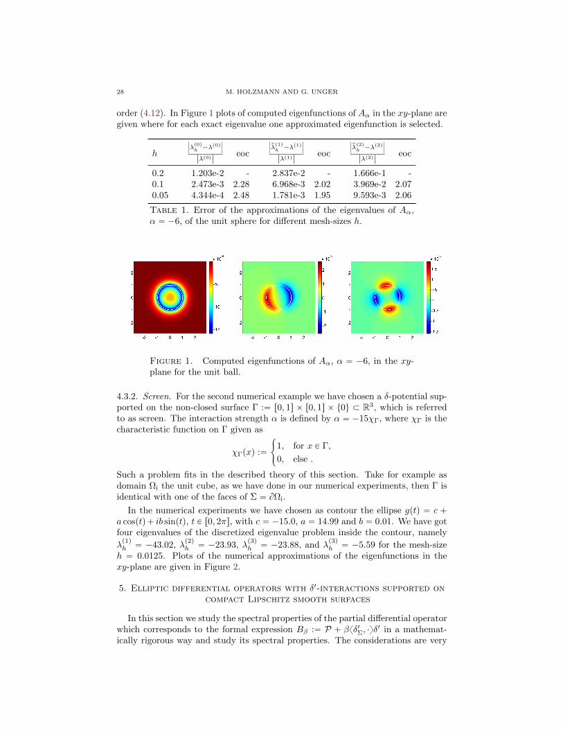
order (4.12). In Figure 1 plots of computed eigenfunctions of Aα in the xy-plane aregiven where for each exact eigenvalue one approximated eigenfunction is selected.
h
ˇ
ˇ
ˇλp0qh ´λp0q
ˇ
ˇ
ˇ
|λp0q|eoc
ˇ
ˇ
ˇ
pλp1qh ´λp1q
ˇ
ˇ
ˇ
|λp1q|eoc
ˇ
ˇ
ˇ
pλp2qh ´λp2q
ˇ
ˇ
ˇ
|λp2q|eoc
0.2 1.203e-2 - 2.837e-2 - 1.666e-1 -0.1 2.473e-3 2.28 6.968e-3 2.02 3.969e-2 2.070.05 4.344e-4 2.48 1.781e-3 1.95 9.593e-3 2.06
Table 1. Error of the approximations of the eigenvalues of Aα,α “ ´6, of the unit sphere for different mesh-sizes h.
Figure 1. Computed eigenfunctions of Aα, α “ ´6, in the xy-plane for the unit ball.
4.3.2. Screen. For the second numerical example we have chosen a δ-potential sup-ported on the non-closed surface Γ :“ r0, 1s ˆ r0, 1s ˆ t0u Ă R3, which is referredto as screen. The interaction strength α is defined by α “ ´15χΓ, where χΓ is thecharacteristic function on Γ given as
χΓpxq :“
#
1, for x P Γ,
0, else .
Such a problem fits in the described theory of this section. Take for example asdomain Ωi the unit cube, as we have done in our numerical experiments, then Γ isidentical with one of the faces of Σ “ BΩi.
In the numerical experiments we have chosen as contour the ellipse gptq “ c `a cosptq` ib sinptq, t P r0, 2πs, with c “ ´15.0, a “ 14.99 and b “ 0.01. We have gotfour eigenvalues of the discretized eigenvalue problem inside the contour, namely
λp1qh “ ´43.02, λ
p2qh “ ´23.93, λ
p3qh “ ´23.88, and λ
p3qh “ ´5.59 for the mesh-size
h “ 0.0125. Plots of the numerical approximations of the eigenfunctions in thexy-plane are given in Figure 2.
5. Elliptic differential operators with δ1-interactions supported oncompact Lipschitz smooth surfaces
In this section we study the spectral properties of the partial differential operatorwhich corresponds to the formal expression Bβ :“ P ` βxδ1Σ, ¨yδ
1 in a mathemat-ically rigorous way and study its spectral properties. The considerations are very
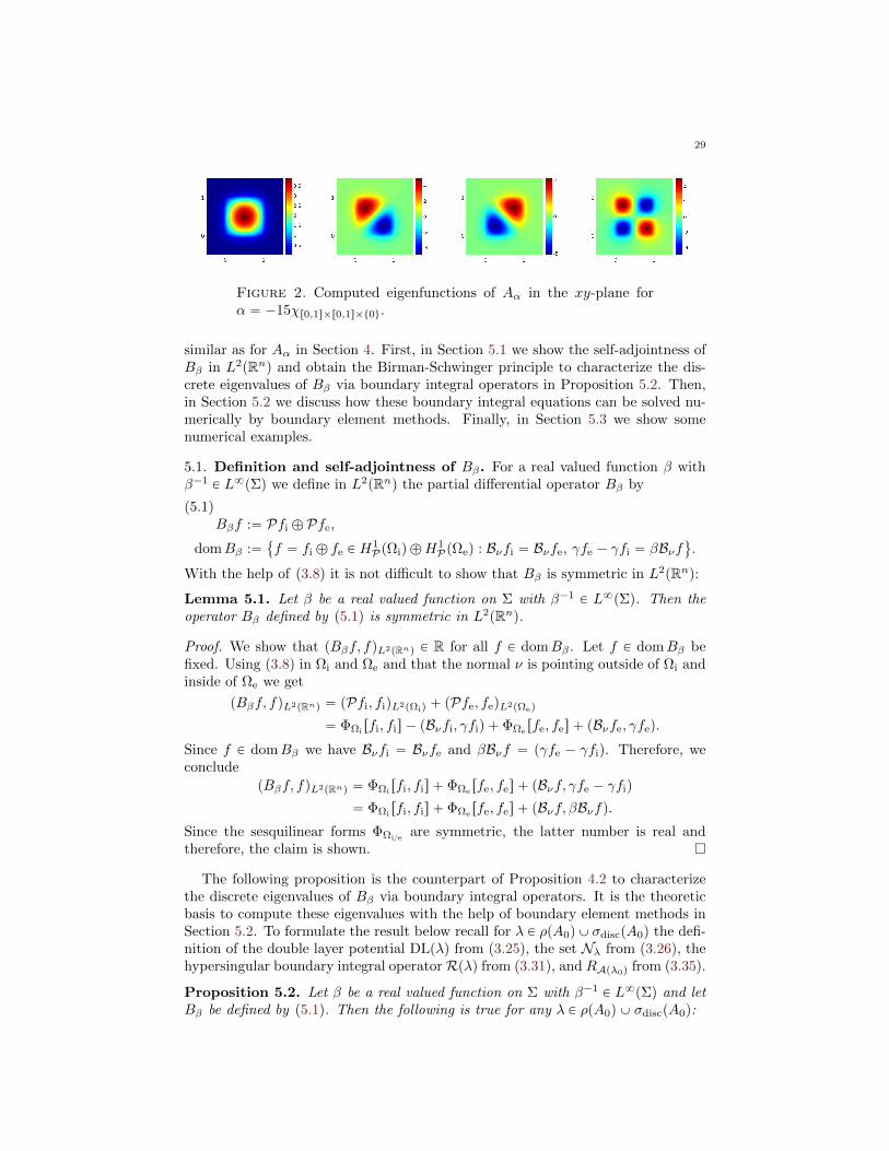
29
Figure 2. Computed eigenfunctions of Aα in the xy-plane forα “ ´15χr0,1sˆr0,1sˆt0u.
similar as for Aα in Section 4. First, in Section 5.1 we show the self-adjointness ofBβ in L2pRnq and obtain the Birman-Schwinger principle to characterize the dis-crete eigenvalues of Bβ via boundary integral operators in Proposition 5.2. Then,in Section 5.2 we discuss how these boundary integral equations can be solved nu-merically by boundary element methods. Finally, in Section 5.3 we show somenumerical examples.
5.1. Definition and self-adjointness of Bβ. For a real valued function β withβ´1 P L8pΣq we define in L2pRnq the partial differential operator Bβ by
Bβf :“ Pfi ‘ Pfe,
domBβ :“
f “ fi ‘ fe P H1PpΩiq ‘H
1PpΩeq : Bνfi “ Bνfe, γfe ´ γfi “ βBνf
(
.
(5.1)
With the help of (3.8) it is not difficult to show that Bβ is symmetric in L2pRnq:
Lemma 5.1. Let β be a real valued function on Σ with β´1 P L8pΣq. Then theoperator Bβ defined by (5.1) is symmetric in L2pRnq.
Proof. We show that pBβf, fqL2pRnq P R for all f P domBβ . Let f P domBβ befixed. Using (3.8) in Ωi and Ωe and that the normal ν is pointing outside of Ωi andinside of Ωe we get
pBβf, fqL2pRnq “ pPfi, fiqL2pΩiq ` pPfe, feqL2pΩeq
“ ΦΩirfi, fis ´ pBνfi, γfiq ` ΦΩe
rfe, fes ` pBνfe, γfeq.
Since f P domBβ we have Bνfi “ Bνfe and βBνf “ pγfe ´ γfiq. Therefore, weconclude
pBβf, fqL2pRnq “ ΦΩirfi, fis ` ΦΩe
rfe, fes ` pBνf, γfe ´ γfiq
“ ΦΩirfi, fis ` ΦΩe
rfe, fes ` pBνf, βBνfq.Since the sesquilinear forms ΦΩie
are symmetric, the latter number is real andtherefore, the claim is shown.
The following proposition is the counterpart of Proposition 4.2 to characterizethe discrete eigenvalues of Bβ via boundary integral operators. It is the theoreticbasis to compute these eigenvalues with the help of boundary element methods inSection 5.2. To formulate the result below recall for λ P ρpA0q Y σdiscpA0q the defi-nition of the double layer potential DLpλq from (3.25), the set Nλ from (3.26), thehypersingular boundary integral operator Rpλq from (3.31), and RApλ0q from (3.35).
Proposition 5.2. Let β be a real valued function on Σ with β´1 P L8pΣq and letBβ be defined by (5.1). Then the following is true for any λ P ρpA0q Y σdiscpA0q:
30 M. HOLZMANN AND G. UNGER
(i) kerpBβ ´λqa kerpA0´λq ‰ t0u if and only if there exists 0 ‰ ϕ P Nλ suchthat pβ´1 `Rpλqqϕ “ 0. Moreover,
(5.2) kerpBβ ´ λq a kerpA0 ´ λq “
DLpλqϕ : ϕ P Nλ, pβ´1 `Rpλqqϕ “ 0
(
.
(ii) If λ P ρpA0q, then λ P σppBβq if and only if 0 P σppβ´1 `Rpλqq.
(iii) kerpBβ ´ λq X kerpA0 ´ λq ‰ t0u if and only if there exists pϕ,ψqJ P
ranRApλ0q such that ψ “ 0.
(iv) If λ R σppBβq Y σpA0q, then β´1 `Rpλq : H12pΣq Ñ H´12pΣq admits abounded and everywhere defined inverse.
Proof. (i) Assume first that kerpBβ ´ λq a kerpA0 ´ λq ‰ t0u and let f P kerpBβ ´λqakerpA0´λq. Then by Lemma 3.5 (i) there exists ϕ P Nλ such that f “ DLpλqϕ.Since f P domBβ one has with Lemma 3.5 (ii)
βBνf “ γfe ´ γfi “ γpDLpλqϕqe ´ γpDLpλqϕqi “ ϕ.
With Bνf “ ´Rpλqϕ this can be rewritten as β´1ϕ “ ´Rpλqϕ. Hence, the aboveconsiderations show
(5.3) kerpBβ ´ λq a kerpA0 ´ λq Ă
DLpλqϕ : ϕ P Nλ, pβ´1 `Rpλqqϕ “ 0
(
.
Conversely, assume that there exists ϕ P Nλ such that pβ´1 ` Rpλqqϕ “ 0.Then f :“ DLpλqϕ P H1
PpRnzΣq is nontrivial by Lemma 3.5 (ii). Using the jumpproperties of DLpλqϕ from Lemma 3.5 (ii) we conclude further Bνfi “ Bνfe and
γfe ´ γfi “ γpDLpλqϕqe ´ γpDLpλqϕqi “ ϕ “ ´βRpλqϕ “ βBνf,
where β´1pI ` βRpλqqϕ “ 0 was used. Hence, f P domBβ . With Lemma 3.5 (i)we conclude with ϕ P Nλ eventually
pBβ ´ λqf “ pP ´ λqpDLpλqϕqi ‘ pP ´ λqpDLpλqϕqe “ 0,
which shows λ P σppBβq and
(5.4)
DLpλqϕ : ϕ P Nλ, pβ´1 `Rpλqqϕ “ 0
(
Ă kerpBβ ´ λq a kerpA0 ´ λq.
Note that (5.3) and (5.4) give (5.2). Hence, all claims in item (i) are proved.
Assertion (ii) is a simple consequence of item (i), as for λ R σpA0q we havekerpA0 ´ λq “ t0u and Nλ “ H12pΣq.
Statement (iii) follows from Theorem 3.8. Note that f P domBβXdomA0 if andonly if f P H2pRnq and Bνf “ β´1pγfe ´ γfiq “ 0. With Theorem 3.8 it followsthat f P kerpBβ´λqXkerpA0´λq if and only if there exists pϕ,ψqJ “ pγf,BνfqJ PranRApλ0q such that ψ “ 0.
(iv) First, we note that the multiplication with the function β´1 P L8pΣq givesrise to a bounded operator from H12pΣq to L2pΣq and as L2pΣq is compactly em-bedded in H´12pΣq, the operator β´1 : H12pΣq Ñ H´12pΣq is compact. There-fore, we deduce from [28, Theorem 2.26] that β´1 `Rpλq : H12pΣq Ñ H´12pΣqis a Fredholm operator with index zero, as Rpλq is a Fredholm operator with in-dex zero by Lemma 3.6 (ii). Since λ is not an eigenvalue of Bβ by assumption,we deduce from (ii) that β´1 ` Rpλq is injective and hence, this operator is alsosurjective. Therefore, it follows from the open mapping theorem that β´1 `Rpλqhas a bounded inverse from H´12pΣq to H12pΣq.
31
In the following proposition we show the self-adjointness of Bβ and a Krein typeresolvent formula for this operator. We remark that the resolvent formula in (5.5)is well defined, as β´1 ` Rpλq : H12pΣq Ñ H´12pΣq is boundedly invertible forλ P ρpA0q X ρpBβq by Proposition 5.2 (iv).
Proposition 5.3. Let β be a real valued function on Σ with β´1 P L8pΣq and letthe operators A0, DLpλq, and Rpλq, λ P ρpA0q, be given by (3.9), (3.25), and (3.31),respectively. Then the operator Bβ defined by (5.1) is self-adjoint in L2pRnq andthe following is true:
(i) For λ P ρpA0q X ρpBβq the resolvent of Bβ is given by
(5.5) pBβ ´ λq´1 “ pA0 ´ λq
´1 `DLpλq`
β´1 `Rpλq˘´1BνpA0 ´ λq
´1.
(ii) σesspBβq “ σesspA0q.
Proof. In order to show that Bβ is self-adjoint, we show that ranpBβ´λq “ L2pRnqfor λ P CzpσpA0q Y σppBβqq. Let f P L2pRnq be fixed and define
g :“ pA0 ´ λq´1f `DLpλq
`
β´1 `Rpλq˘´1BνpA0 ´ λq
´1f.
Note that g is well defined, as β´1`Rpλq : H12pΣq Ñ H´12pΣq admits a boundedinverse for λ R σpA0q Y σppBβq by Proposition 5.2 (iv). We are going to show thatg P domBβ and pBβ ´ λqg “ f . This shows then ranpBβ ´ λq “ L2pRnq andalso (5.5).
Since pA0´λq´1f P H2pRnq by Proposition 3.2 implies BνpA0´λq
´1f P L2pΣq ĂH´12pΣq, we conclude from Proposition 5.2 (iv) and Lemma 3.5 that
DLpλq`
β´1 `Rpλq˘´1BνpA0 ´ λq
´1f P H1PpRnzΣq.
Therefore, also g P H1PpRnzΣq. Moreover, we get with the help of Lemma 3.5 (ii)
that Bνge “ Bνgi. Applying once more Lemma 3.5 (ii) we conclude
β´1pγge ´ γgiq ´ Bνg “ β´1`
β´1 `Rpλq˘´1BνpA0 ´ λq
´1f ´ BνpA0 ´ λq´1f
`Rpλq`
β´1 `Rpλq˘´1BνpA0 ´ λq
´1f “ 0,
which shows g P domBβ . Next, we have with ϕ :“ pβ´1 `Rpλqq´1BνpA0 ´ λq´1f
pBβ ´ λqg “ pP ´ λqpA0 ´ λq´1f ` pP ´ λqpDLpλqϕqi ‘ pP ´ λqpDLpλqϕqe “ f,
where (3.27) was used in the last step. With the previous considerations we deducenow the self-adjointness of Bβ and (5.5).
It remains to show assertion (ii). Let λ P CzR be fixed. Due to the mappingproperties of the resolvent of A0 from Proposition 3.2 and the mapping propertiesof Bν from (3.7) the operator
BνpA0 ´ λq´1 : L2pRnq Ñ L2pΣq Ñ H´12pΣq
is bounded. Hence, Proposition 5.2 (iv) yields that`
β´1 `Rpλq˘´1BνpA0 ´ λq
´1 : L2pRnq Ñ H12pΣq
is bounded. As H12pΣq is compactly embedded in L2pΣq we conclude that thelatter operator is compact from L2pRnq to L2pΣq. Since DLpλq : L2pΣq Ñ L2pRnqis bounded by (3.25), we find eventually that
pBβ ´ λq´1 ´ pA0 ´ λq
´1 “ DLpλq`
β´1 `Rpλq˘´1BνpA0 ´ λq
´1
32 M. HOLZMANN AND G. UNGER
is compact in L2pRnq. Therefore, we get with the Weyl theorem σesspBβq “σesspA0q.
The following result is the counterpart of Proposition 4.4 on the inverse of theBirman-Schwinger operator β´1 ` Rpλq, which will be of great importance forthe numerical calculation of the discrete eigenvalues of Bβ via boundary elementmethods.
Proposition 5.4. Let β be a real valued function with β´1 P L8pΣq and let Bβ bedefined by (5.1). Then the map
ρpBβq X ρpA0q Q λ ÞÑ`
β´1 `Rpλq˘´1
can be extended to a holomorphic operator-valued function, which is holomorphicin ρpBβq with respect to the toplogy in BpH´12pΣq, H12pΣqq. Moreover, for λ0 R
σesspBβq “ σesspA0q one has kerpBβ ´ λ0q a kerpA0 ´ λ0q ‰ t0u if and only ifpβ´1 `Rpλqq´1 has a pole at λ0 and
(5.6) kerpBβ´λ0qakerpA0´λ0q “
DLpλ0qϕ : limλÑλ0
pλ´λ0qpβ´1`Rpλqq´1ϕ ‰ 0
(
.
Proof. The proof is similar as the proof of Proposition 4.4 and split into 3 steps.
Step 1: Define the map
rγsΣ : H1PpRnzΣq Ñ H12pΣq, rγsΣf :“ γfe ´ γfi.
Let λ P ρpBβq X ρpA0q be fixed. We show that
(5.7)`
β´1 `Rpλq˘´1
“ rγsΣpBβ ´ λq´1rγs˚Σ.
In particular, with Proposition 5.2 (iv) this implies that rγsΣpBβ´λq´1rγsΣ belongs
to BpH´12pΣq, H12pΣqq. To show (5.7) we note first that rγsΣf “ βBνf holds forf P domBβ and hence (5.5) implies
rγsΣpBβ ´ λq´1 “ βBνpBβ ´ λq´1
“ βBνpA0 ´ λq´1 ´ βRpλq
`
β´1 `Rpλq˘´1BνpA0 ´ λq
´1
“ β“`
β´1 `Rpλq˘
´Rpλq‰`
β´1 `Rpλq˘´1BνpA0 ´ λq
´1
“`
β´1 `Rpλq˘´1BνpA0 ´ λq
´1,
which implies, after taking the dual,
pBβ ´ λq´1rγs˚Σ “ DLpλq
`
β´1 `Rpλq˘´1
.
In particular, by Lemma 3.5 and Proposition 5.2 (iv) the right hand side belongsto BpH´12pΣq, H1
PpRnzΣqq and thus the same must be true for pBβ ´ λq´1rγs˚Σ.Therefore, we are allowed to apply rγsΣ and the last formula shows, with the helpof Lemma 3.5 (ii), the relation (5.7).
Step 2: We show that rγsΣpBβ ´ λq´1rγs˚Σ P BpH´12pΣq, H12pΣqq for anyλ P ρpBβq and that the mapping ρpBβq Q λ ÞÑ rγsΣpBβ ´ λq
´1rγs˚Σ is holomorphic
in BpH´12pΣq, H12pΣqq.
First, we note that domBβ Ă H1PpRnzΣq implies that
pBβ ´ λq´1 P BpL2pRnq, H1
PpRnzΣqq,
33
see (3.16) for a similar argument. Hence, by duality also
pBβ ´ λq´1 P BppH1
PpRnzΣqq˚, L2pRnqq.
With the resolvent identity this implies for any λ0 P ρpBβq and λ P ρpBβq X ρpA0q,in a similar way as in the proof of Proposition 3.2, that
rγsΣpBβ ´ λ0q´1rγs˚Σ ´ rγsΣpBβ ´ λq
´1rγs˚Σ
“ pλ0 ´ λqrγsΣpBβ ´ λ0q´1pBβ ´ λq
´1rγs˚Σ,
which shows first with (5.7) that rγsΣpBβ´λ0q´1rγs˚Σ P BpH´12pΣq, H12pΣqq and
in a second step, that rγsΣpBβ´λq´1rγs˚Σ is holomorphic in BpH´12pΣq, H12pΣqq,
which shows the claim of this step.
Step 3: Finally, it follows from Proposition 5.2 (i) that kerpBβ ´ λ0q a kerpA0 ´
λ0q ‰ t0u if and only if there exists ϕ P Nλ0such that pβ´1 `Rpλ0qqϕ “ 0, i.e. if
and only if λ ÞÑ pβ´1`Rpλqq´1 has a pole at λ0. This shows immediately (5.6).
5.2. Numerical approximation of discrete eigenvalues of Bβ. The approx-imation of the discrete eigenvalues of Bβ by boundary element methods is basedon the same principles as those for the discrete eigenvalues of Aα described in Sec-tion 4.2. In order to apply boundary element methods for the approximation of thediscrete eigenvalues of Bβ it is necessary to have an integral representation of theparamatrix Gpλq of P ´ λ or at least a good approximation of the boundary inte-gral operator Rpλq. We use the characterization of the discrete eigenvalues of Bβ interms of boundary integral operators given in Proposition 5.2 and Proposition 5.4.The discrete eigenvalues split into the eigenvalues of the nonlinear eigenvalue prob-lem
(5.8) pβ´1 `Rpλqqψ “ 0
in ρpA0q and into distinct discrete eigenvalues of A0 which are either the poles ofAp¨q satisfying the properties specified in Proposition 5.2 (iii) or poles of pβ´1 `
Rp¨qq´1 in σdiscpA0q.
In the following presentation of the boundary element method we want to con-sider first the case that σdiscpA0q “ ∅ and then the general case. If σdiscpA0q “ ∅,then the discrete eigenvalues of Bβ coincide with the eigenvalues of the nonlineareigenvalue problem (5.8) in ρpA0q as shown in Proposition 5.2 (ii). In this situationa complete convergence analysis is provided by the theory of Section 2. For thegeneral case the convergence of the approximations of the discrete eigenvalues ofBβ which lie in σdiscpA0q is an open issue.
The discretized problems for the approximation of the discrete eigenvalues of Bβwhich result from the approximations of the boundary integral operators by bound-ary element methods are problems for the determination of poles of meromorphicmatrix-valued functions. For this kind of problems we suggest the contour integralmethod [10], which was discussed in Section 4.2.1.
5.2.1. Approximation of discrete eigenvalues of Bα for the case σdiscpA0q “ ∅.For σdiscpA0q “ ∅ the discrete eigenvalues of Bβ coincide, according to Propo-sition 5.2 (ii), with the eigenvalues of the eigenvalue problem for pβ´1 ` Rp¨qq.Lemma 3.6 (iii) shows that the map ρpA0q Q λ ÞÑ pβ´1 ` Rpλqq is holomorphicin BpH12pΣq, H´12pΣqq. Moreover, by Lemma 3.6 (i) the operators β´1 `Rpλq
34 M. HOLZMANN AND G. UNGER
satisfy for λ P ρpA0q Garding’s inequality of the form (2.1). Hence, any conform-ing Galerkin method for the approximation of the eigenvalue problem (5.8) is aconvergent method, which follows from the theory in Section 2.
For the boundary element approximation of the eigenvalue problem (5.8) we firstassume that Ωi is a polyhedral Lipschitz domain. The case of general Lipschitz do-mains is addressed in Remark 5.6. Let pTN qNPN be a sequence of quasi-uniformtriangulations of Ωi with the properties specified in (4.9). As approximation spacefor the approximation of the eigenfunctions of the eigenvalue problem (5.8) wechoose the space S1pTN q of piecewise linear functions with respect to the triangu-lation TN . The approximation property of S1pTN q depends on the regularity of thefunctions which are approximated. In order to measure the regularity of functionsdefined on a piecewise smooth boundary Σ, partitioned by open sets Σ1, . . . ,ΣJsuch that
Σ “Jď
j“1
Σj , Σj X Σi “ ∅ for i ‰ j,
so-called piecewise Sobolev spaces of order s ą 1 defined by
HspwpΣq :“ tv P H1pΣq : v æ Σj P H
spΣjq for j “ 1, . . . , Ju
are used, see [31, Definition 4.1.48]. For s P r0, 1s the space HspwpΣq is defined by
HspwpΣq :“ HspΣq. If W is a finite dimensional subspace of H
12`spw pΣq for s P p0, 3
2 s,then
(5.9) δH12pΣqpW,S1pTN qq “ supwPW
wH12pΣq
“1
infψNPS1pTN q
w ´ ψN H12pΣq “ OphpNqsq
holds [31, Proposition 4.1.50].
The Galerkin approximation of the eigenvalue problem (5.8) reads as follows:find eigenvalues λN P C and corresponding eigenfunctions ψN P S1pTN qzt0u suchthat
(5.10)`
pβ´1 `RpλN qqψN , χN˘
“ 0 @χN P S1pTN q.
We can apply all convergence results from Theorem 2.1 to the Galerkin eigenvalueproblem (5.10). In the following theorem the asymptotic convergence order ofthe approximations of the eigenvalues and the corresponding eigenfunctions arespecified.
Theorem 5.5. Let D Ă ρpA0q be a compact and connected set in C such that BD is
a simple rectifiable curve. Suppose that λ P D is the only eigenvalue of pβ´1`Rp¨qqin D and that kerpβ´1 `Rpλqq Ă H
12`spw pΣq for some s P p0, 3
2 s. Then there existan N0 P N and a constant c ą 0 such that for all N ě N0 we have:
(i) For all eigenvalues λN of the Galerkin eigenvalue problem (5.10) in D
(5.11) |λ´ λN | ď cphpNqq2s
holds.(ii) If pλN , uN q is an eigenpair of (5.10) with λN P D and ψN H12pΣq “ 1,
then
(5.12) infψPkerpβ´1`Rpλqq
ψ ´ ψN H12pΣq ď c p|λN ´ λ| ` phpNqqsq .
35
Proof. We have shown in Lemma 3.6 (iii) that the map ρpA0q Q λ ÞÑ pβ´1`Rpλqq isholomorphic in BpH12pΣq, H´12pΣqq. Moreover, by Lemma 3.6 (i), the operatorsβ´1 ` Rpλq satisfy for λ P ρpA0q Garding’s inequality of the form (2.1). TheGalerkin approximation (5.10) of the eigenvalue problem for pβ´1 ` Rp¨qq is aconforming approximation since S1pTN q is a subspace of H12pΣq. Hence, we canuse Theorem 2.1. The error estimates follows from the approximation property (5.9)of S1pTN q and the fact, that the eigenfunction of the adjoint problem are as regularas for pβ´1 `Rp¨qq.
Remark 5.6. If Ω is a bounded Lipschitz domain with a curved piecewise C2-boundary the approximation of the boundary by a triangulation with flat trianglesas described in [31, Chapter 8] reduces the maximal possible convergence order sfor the error of the eigenvalues in (5.11) and for the error of the eigenfunctionsin (5.12) from s “ 3
2 to s “ 1. This follows from the results of the discretization ofboundary integral operators for approximated boundaries [31, Chapter 8] and fromthe abstract results of eigenvalue problem approximations [21,22].
5.2.2. Approximation of discrete eigenvalues of Bα for the case σdiscpA0q ‰ ∅. IfσdiscpA0q ‰ ∅, then Proposition 5.2 and Proposition 5.4 imply that the discreteeigenvalues of Bβ are poles of pβ´1`Rp¨qq´1 or poles of Ap¨q with the property givenin Proposition 5.2 (iii). These characterizations are used for the approximation ofthe discrete eigenvalues of Bβ . We will separately discuss both cases.
Let λ0 be a discrete eigenvalue of Bβ and in addition be a pole of pβ´1`Rp¨qq´1.Then pβ´1 `Rp¨qq is either holomorphic in λ0, which is the case for λ0 P ρpA0q, orλ0 is a pole of pβ´1`Rp¨qq. A pole λ0 P ρpA0q of pβ´1`Rp¨qq´1 can be consideredas an eigenvalue of the eigenvalue problem for the homomorphic Fredholm operator-valued function pβ´1`Rp¨qq in ρpA0q and the convergence results of Section 2 canbe applied with the same reasoning as in the case of σdiscpA0q “ ∅. If λ0 P σdiscpA0q
is a pole of pβ´1`Rp¨qq, then the convergence theory of Section 2 is not applicablefor λ0. We expect convergence of the approximations for this kind of poles ofpβ´1 `Rp¨qq´1, but a rigorous numerical analysis has not established so far.
The approximation of a discrete eigenvalue λ0 of Bβ which is not a pole ofpβ´1`Rp¨qq´1 is based on the following characterization from Proposition 5.2 (iii):λ0 is a pole of Ap¨q and there exists a pair p0, 0q ‰ pψ,ϕq P H12pΣq ˆ H´12pΣqsuch that
(5.13) Apλq´1
ˆ
ψϕ
˙
“
ˆ
00
˙
and ψ “ 0.
For the approximation of the eigenvalues of the nonlinear eigenvalue problem in (5.13)formally the Galerkin problem in S1pTN qˆS0pTN q as given in (4.14) is considered.If the contour integral method is used for the computations of the approximationsof the eigenvalues for Ap¨q´1, then Ap¨q´1 does not have not be computed, butinstead its inverse Ap¨q. The convergence theory of Section 2 can be applied tothe approximation of those eigenvalues of Ap¨q´1 for which Ap¨q´1 is holomorphic.If λ0 is a pole Ap¨q and of Ap¨q´1, we again expect convergence, but a numericalanalysis for such kind of poles has not been provided so far.
5.3. Numerical examples. For the numerical examples of the approximation ofdiscrete eigenvalues of Bβ we choose P “ ´∆. In this case σesspA0q “ r0,8q,
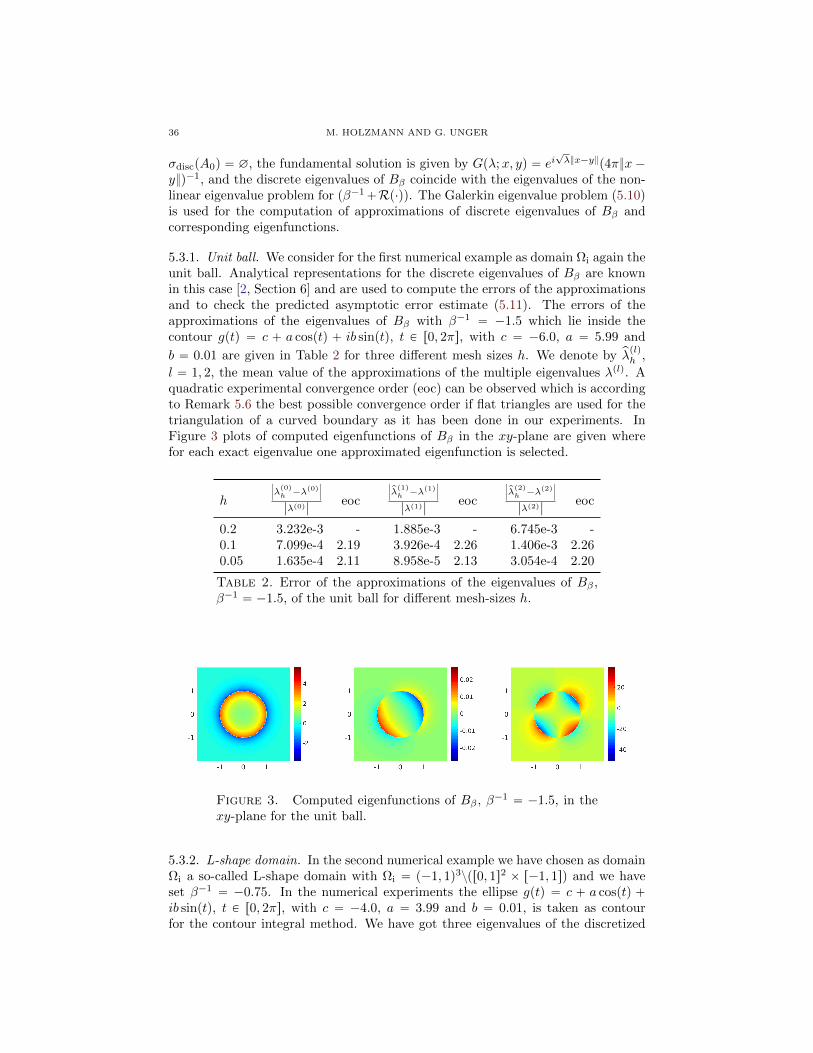
36 M. HOLZMANN AND G. UNGER
σdiscpA0q “ ∅, the fundamental solution is given by Gpλ;x, yq “ ei?λx´yp4πx´
yq´1, and the discrete eigenvalues of Bβ coincide with the eigenvalues of the non-linear eigenvalue problem for pβ´1`Rp¨qq. The Galerkin eigenvalue problem (5.10)is used for the computation of approximations of discrete eigenvalues of Bβ andcorresponding eigenfunctions.
5.3.1. Unit ball. We consider for the first numerical example as domain Ωi again theunit ball. Analytical representations for the discrete eigenvalues of Bβ are knownin this case [2, Section 6] and are used to compute the errors of the approximationsand to check the predicted asymptotic error estimate (5.11). The errors of theapproximations of the eigenvalues of Bβ with β´1 “ ´1.5 which lie inside thecontour gptq “ c ` a cosptq ` ib sinptq, t P r0, 2πs, with c “ ´6.0, a “ 5.99 and
b “ 0.01 are given in Table 2 for three different mesh sizes h. We denote by pλplqh ,
l “ 1, 2, the mean value of the approximations of the multiple eigenvalues λplq. Aquadratic experimental convergence order (eoc) can be observed which is accordingto Remark 5.6 the best possible convergence order if flat triangles are used for thetriangulation of a curved boundary as it has been done in our experiments. InFigure 3 plots of computed eigenfunctions of Bβ in the xy-plane are given wherefor each exact eigenvalue one approximated eigenfunction is selected.
h
ˇ
ˇ
ˇλp0qh ´λp0q
ˇ
ˇ
ˇ
|λp0q|eoc
ˇ
ˇ
ˇ
pλp1qh ´λp1q
ˇ
ˇ
ˇ
|λp1q|eoc
ˇ
ˇ
ˇ
pλp2qh ´λp2q
ˇ
ˇ
ˇ
|λp2q|eoc
0.2 3.232e-3 - 1.885e-3 - 6.745e-3 -0.1 7.099e-4 2.19 3.926e-4 2.26 1.406e-3 2.260.05 1.635e-4 2.11 8.958e-5 2.13 3.054e-4 2.20
Table 2. Error of the approximations of the eigenvalues of Bβ ,β´1 “ ´1.5, of the unit ball for different mesh-sizes h.
Figure 3. Computed eigenfunctions of Bβ , β´1 “ ´1.5, in thexy-plane for the unit ball.
5.3.2. L-shape domain. In the second numerical example we have chosen as domainΩi a so-called L-shape domain with Ωi “ p´1, 1q3zpr0, 1s2 ˆ r´1, 1sq and we haveset β´1 “ ´0.75. In the numerical experiments the ellipse gptq “ c ` a cosptq `ib sinptq, t P r0, 2πs, with c “ ´4.0, a “ 3.99 and b “ 0.01, is taken as contourfor the contour integral method. We have got three eigenvalues of the discretized
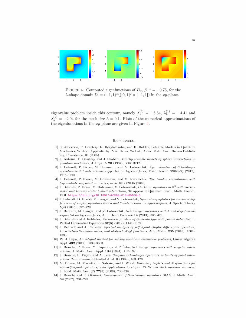
37
Figure 4. Computed eigenfunctions of Bβ , β´1 “ ´0.75, for theL-shape domain Ωi “ p´1, 1q3zpr0, 1s2 ˆ r´1, 1sq in the xy-plane.
eigenvalue problem inside this contour, namely λp0qh “ ´5.54, λ
p1qh “ ´4.41 and
λp2qh “ ´2.94 for the mesh-size h “ 0.1. Plots of the numerical approximations of
the eigenfunctions in the xy-plane are given in Figure 4.
References
[1] S. Albeverio, F. Gesztesy, R. Høegh-Krohn, and H. Holden, Solvable Models in Quantum
Mechanics. With an Appendix by Pavel Exner, 2nd ed., Amer. Math. Soc. Chelsea Publish-ing, Providence, RI (2005).
[2] J. Antoine, F. Gesztesy and J. Shabani, Exactly solvable models of sphere interactions in
quantum mechanics, J. Phys. A 20 (1987), 3687–3712.[3] J. Behrndt, P. Exner, M. Holzmann, and V. Lotoreichik, Approximation of Schrodinger
operators with δ-interactions supported on hypersurfaces, Math. Nachr. 290(8-9) (2017),
1215–1248.[4] J. Behrndt, P. Exner, M. Holzmann, and V. Lotoreichik, The Landau Hamiltonian with
δ-potentials supported on curves, arxiv:1812.09145 (2018).
[5] J. Behrndt, P. Exner, M. Holzmann, V. Lotoreichik, On Dirac operators in R3 with electro-static and Lorentz scalar δ-shell interactions, To appear in Quantum Stud.: Math. Found.,
DOI: https://doi.org/10.1007/s40509-019-00186-6.
[6] J. Behrndt, G. Grubb, M. Langer, and V. Lotoreichik, Spectral asymptotics for resolvent dif-ferences of elliptic operators with δ and δ1-interactions on hypersurfaces, J. Spectr. Theory5(4) (2015), 697–729.
[7] J. Behrndt, M. Langer, and V. Lotoreichik, Schrodinger operators with δ and δ1-potentials
supported on hypersurfaces, Ann. Henri Poincare 14 (2013), 385–423.
[8] J. Behrndt and J. Rohleder, An inverse problem of Calderon type with partial data, Comm.Partial Differential Equations 37(6) (2012), 1141–1159.
[9] J. Behrndt and J. Rohleder, Spectral analysis of selfadjoint elliptic differential operators,Dirichlet-to-Neumann maps, and abstract Weyl functions, Adv. Math. 285 (2015), 1301–1338.
[10] W. J. Beyn, An integral method for solving nonlinear eigenvalue problems, Linear Algebra
Appl. 432 (2012), 3839–3863.
[11] J. Brasche, P. Exner, Y. Kuperin, and P. Seba, Schrodinger operators with singular inter-
actions, J. Math. Anal. Appl. 184 (1994), 112–139.[12] J. Brasche, R. Figari, and A. Teta, Singular Schrodinger operators as limits of point inter-
action Hamiltonians, Potential Anal. 8 (1998), 163–178.
[13] M. Brown, M. Marletta, S. Naboko, and I. Wood, Boundary triplets and M-functions fornon-selfadjoint operators, with applications to elliptic PDEs and block operator matrices,
J. Lond. Math. Soc. (2) 77(3) (2008), 700–718.
[14] J. Brasche and K. Ozanova, Convergence of Schrodinger operators, SIAM J. Math. Anal.39 (2007), 281–297.
38 M. HOLZMANN AND G. UNGER
[15] P. Exner, Leaky quantum graphs: a review, in: Analysis on graphs and its applications.
Selected papers based on the Isaac Newton Institute for Mathematical Sciences programme,
Cambridge, UK, 2007. Proc. Symp. Pure Math. 77 (2008), 523–564.[16] P. Exner and H. Kovarık, Quantum Waveguides. Theoretical and Mathematical Physics,
Springer (2015).
[17] P. Exner and K. Nemcova, Leaky quantum graphs: approximations by point-interactionHamiltonians, J. Phys. A 36 (2003), 10173–10193.
[18] A. Figotin and P. Kuchment, Band-gap structure of spectra of periodic dielectric and acous-
tic media. II. Two-dimensional photonic crystals, SIAM J. Appl. Math. 56(6) (1996), 1561–1620.
[19] I. C. Gohberg, S. Goldberg, M. A. Kaashoek, Classes of Linear Operators. Vol. I. Birkhauser
Verlag, Basel (1990).[20] I. C. Gohberg and E. I. Sigal, An operator generalization of the logarithmic residue theorem
and Rouche’s theorem, Math. USSR-Sb. 13 (1971), 603–625.[21] O. Karma, Approximation in eigenvalue problems for holomorphic Fredholm operator func-
tions. I, Numer. Funct. Anal. Optim. 17 (1996), 365–387.
[22] O. Karma, Approximation in eigenvalue problems for holomorphic Fredholm operator func-tions. II. (Convergence rate) , Numer. Funct. Anal. Optim. 17 (1996), 389–408.
[23] T. Kato, Perturbation theory for linear operators. Springer-Verlag, Berlin, reprint of the
1980 edition (1995).[24] A. Kimeswenger, O. Steinbach, and G. Unger, Coupled finite and boundary element methods
for fluid-solid interaction eigenvalue problems, SIAM J. Numer. Anal. 52(5) (2014), 2400–
2414.[25] A. Kleefeld, A numerical method to compute interior transmission eigenvalues, Inverse
Problems 29(10) (2013), 104012, 20.
[26] V. Kozlov and V. Maz1ya, Differential Equations with Operator Coefficients with Applica-tions to Boundary Value Problems for Partial Differential Equations. Springer-Verlag, Berlin
(1999).[27] R. de L. Kronig and W. Penney, Quantum mechanics of electrons in crystal lattices, Proc.
Roy. Soc. Lond. 130 (1931), 499–513.
[28] W. McLean, Strongly Elliptic Systems and Boundary Integral Equations, Cambridge Uni-versity Press, Cambridge (2000).
[29] A. Mantile, A. Posilicano, and M. Sini, Self-adjoint elliptic operators with boundary condi-
tions on not closed hypersurfaces, J. Differential Equations 261(1) (2016), 1–55.[30] K. Ozanova, Approximation by point potentials in a magnetic field, J. Phys. A 39 (2006),
3071–3083.
[31] S. A. Sauter and C. Schwab, Boundary element methods. Springer-Verlag, Berlin (2011).
[32] W. Smigaj, S. Arridge, T. Betcke , J. Phillips, and J. Schweiger, Solving Boundary Integral
Problems with BEM++, ACM Trans. Math. Software 41(6) (2015), 1–40.[33] O. Steinbach, Numerical approximation methods for elliptic boundary value problems. Finite
and boundary elements. Springer, New York (2008).[34] 0. Steinbach and G. Unger, Convergence analysis of a Galerkin boundary element method
for the Dirichlet Laplacian eigenvalue problem, SIAM J. Numer. Anal. 50 (2012), 710–728.[35] L. H. Thomas, The interaction between a neutron and a proton and the structure of H3,
Phys. Rev., II. Ser. 47 (1935), 903–909.
[36] G. Unger, Analysis of Boundary Element Methods for Laplacian Eigenvalue Problems. PhD
thesis, Graz University of Technology, Graz, 2009.
Institut fur Angewandte Mathematik, Technische Universitat Graz, Steyrergasse 30,
8010 Graz, Austria, E-mail: [email protected]
Institut fur Angewandte Mathematik, Technische Universitat Graz, Steyrergasse 30,8010 Graz, Austria, E-mail: [email protected]
Erschienene Preprints ab Nummer 2015/1
2015/1 O. Steinbach: Space-time finite element methods for parabolic problems2015/2 O. Steinbach, G. Unger: Combined boundary integral equations for acoustic
scattering-resonance problems problems.2015/3 C. Erath, G. Of, F.–J. Sayas: A non-symmetric coupling of the finite volume method
and the boundary element method2015/4 U. Langer, M. Schanz, O. Steinbach, W.L. Wendland (eds.): 13th Workshop on Fast
Boundary Element Methods in Industrial Applications, Book of Abstracts2016/1 U. Langer, M. Schanz, O. Steinbach, W.L. Wendland (eds.): 14th Workshop on Fast
Boundary Element Methods in Industrial Applications, Book of Abstracts2016/2 O. Steinbach: Stability of the Laplace single layer boundary integral operator in
Sobolev spaces2017/1 O. Steinbach, H. Yang: An algebraic multigrid method for an adaptive space-time
finite element discretization2017/2 G. Unger: Convergence analysis of a Galerkin boundary element method for electro-
magnetic eigenvalue problems2017/3 J. Zapletal, G. Of, M. Merta: Parallel and vectorized implementation of analytic
evaluation of boundary integral operators2017/4 S. Dohr, O. Steinbach: Preconditioned space-time boundary element methods for the
one-dimensional heat equation2017/5 O. Steinbach, H. Yang: Comparison of algebraic multigrid methods for an adaptive
space–time finite element discretization of the heat equation in 3D and 4D2017/6 S. Dohr, K. Niino, O. Steinbach: Preconditioned space-time boundary element meth-
ods for the heat equation2017/7 O. Steinbach, M. Zank: Coercive space-time finite element methods for initial bound-
ary value problems2017/8 U. Langer, M. Schanz, O. Steinbach, W.L. Wendland (eds.): 15th Workshop on Fast
Boundary Element Methods in Industrial Applications, Book of Abstracts2018/1 U. Langer, M. Schanz, O. Steinbach, W.L. Wendland (eds.): 16th Workshop on Fast
Boundary Element Methods in Industrial Applications, Book of Abstracts2018/2 S. Dohr, J. Zapletal, G. Of, M. Merta, M. Kravcenko: A parallel space-time boundary
element method for the heat equation2018/3 S. Dohr, M. Merta, G. Of, O. Steinbach, J. Zapletal: A parallel solver for a precondi-
tioned space-time boundary element method for the heat equation2018/4 S. Amstutz, P. Gangl: Toplogical derivative for nonlinear magnetostatic problem2018/5 O. Steinbach, M. Zank: A Stabilized Space–Time Finite Element Method for the
Wave Equation2018/6 O. Steinbach, H. Yang: A Space-Time Finite Element Method for the Linear Bidomain
Equations2018/7 O. Steinbach, M. Zank: Coercive space-time finite element methods for initial bound-
ary value problems2018/8 S. Dohr, K. Niino, O. Steinbach: Space-time boundary element methods for the heat
equation2018/8 O. Steinbach, H. Yang: Space-time finite element methods for parabolic evolution
equations: Discretization, a posteriori error estimation, adaptivity and solution2019/1 O. Steinbach (eds.): 15th Austrian Numerical Analysis Day, Book of Abstracts
2019/2 P. Gangl, K. Sturm: A simplified derivation technique of topological derivatives forquasi-linear transmission problems
2019/3 M. Merkel, P. Gangl, S. Schöps: Shape Optimization of Rotating Electric Machinesusing Isogeometric Analysis and Harmonic Stator-Rotor Coupling
2019/4 P. Gangl and K. Sturm: Asymptotic analysis and topological derivative for 3D quasi-linear magnetostatics