Embed Size (px)
Citation preview
TECHNISCHE UNIVERSITAT MUNCHEN
Institut fur Informatik
Lehrstuhl fur Informatik XVIII
A Study ofResource Allocation Methods
in Virtualized Enterprise Data Centres
Dipl.-Inf. Univ. Alexander Stage
Vollstandiger Abdruck der von der Fakultat fur Informatik der Technischen
Universitat Munchen zur Erlangung des akademischen Grades eines
Doktors der Naturwissenschaften (Dr. rer. nat.)
genehmigten Dissertation.
Vorsitzender: Univ.-Prof. Dr. Florian Matthes
Prufer der Dissertation: 1. Univ.-Prof. Dr. Martin Bichler
2. Univ.-Prof. Dr. Arno Jacobsen
3. Univ.-Prof. Dr. Thomas Setzer,
Karlsruher Institut fur Technologie
Die Dissertation wurde am 14.05.2013 bei der Technischen Universitat
Munchen eingereicht und durch die Fakultat fur Informatik am 13.09.2013
angenommen.
Abstract
In the past, enterprise applications used to be hosted on dedicated physical
servers in data centres. The trend to rely on inexpensive, but computational
powerful commodity hardware has lead to operational inefficiencies caused
by resource demand patterns, non-stationary and high levels of volatility in-
duced by business working hours. To overcome these issues, shared infrastruc-
tures enabled by virtualization technologies have emerged. While a plethora
of approaches have been proposed for shared infrastructure management, a
performance comparison of the methods does not exist. The thesis at hand
provides insights on the competitiveness of static server consolidation and re-
source overbooking in comparison to reactive control for dynamic workload
management. By exercising a large set of experiments, we investigate on the
impact of control system parameters on operational efficiency and application
response times. Even though we are able to determine parameter settings
that lead to high levels of efficiency and to reduce costly virtual machine live
migrations substantially for all benchmark scenarios, static consolidation in
combination with overbooking is found to be preferable.
ii

Zusammenfassung
In der Vergangenheit wurden betriebliche Anwedungen in Rechenzentren auf
dedizierter Hardware betrieben. Durch den Trend zur Nutzung von gunstiger
und leistungsfahiger Hardware, die fur den Massenmarkt produziert wird,
wurde der Rechenzentrumsbetrieb ineffizient. Grund dafur sind nichtsta-
tionare Muster in der Ressourcennachfrage und hohe Grade an Volatilitat,
verursacht durch typische Geschafts- und Arbeitszeiten. Im Gegenzug wur-
den Infrastrukturen aufgebaut, die mit Hilfe von Virtualisierungstechnolo-
gie geteilt nutzbar sind. Obwohl eine Vielzahl von Verwaltungsmechansimen
fur diese Infrastrukturen existieren, ist es bis heute weitgehend unbekannt,
ob dynamische oder statische Ansatze Vorteile bieten. Die vorliegende Ar-
beit beschaftigt sich mit dieser Fragestellung anhand von Experimenten,
die in einem realen Rechenzentrum durchgefuhrt wurden. Unter zu Hilfe-
nahme einer betrachtlichen Menge von Experimenten werden die Auswirkun-
gen von Konrolsystemparameterauspragungen auf operationale Effizienz und
Anwendungsantwortzeiten studiert. Obwohl es moglich ist hohe Effizien-
grade zu erziehlen und kostspielige Live-Migrationen von virtuellen Maschinen
substantiell zu reduzieren, ist statische Konsolidierung in Kombination mit
Uberbuchung fur viele Testszenarien zu bevorzgen.
iii

Acknowledgments
Time rushes by rapidly when I am starting to think about the last years of my
life. Recalling the past struggles, I do see strong reason to focus on the future.
In this spirit I will try to keep the acknowledgments as short as possible. By
doing so, I do not explicitly exclude anybody who helped me on my woebegone
path to finishing this piece of work, but concentrate on the people who bestow
the power on me to overcome the difficulties and disappointments that lie
behind me. I do apologize for any omissions, the fault is completely mine.
First and foremost, I owe Mari, Emma and Ida my deepest, earnest and most
affectionate debt of gratitude. I will always love you for your support, your
indulgence and your willingness to sacrifice so much time, in particular time
you would have wanted to spend with me rather than sharing me with my quest
for consolidated scientific truth. Sometimes it seems to me inconceivable how
you could possibly follow me with tender and loving care without loosing faith.
Hence, I would like to ask you to take this piece of writing as a faithful promise.
From the day I finish this thesis, I will be the spouse and father you deserve
so much more than the humble, distracted and weary being I was, especially
during the last two and a half attritional years.
I am also thankful for the support and care my family accorded me. By now
I consider my family to include my mother Roswitha, my father Wolfgang,
my two twin sisters Annabell and Isabell as well as Mari’s mother Ioanna, her
sister Christine, her grandmother Anka and all other members of her family
iv

I was honored to get to know. Given your indulgence, I hope I am nothing
short of exceeding your expectations.
My most sincere expression of gratitude goes to Prof. Dr. Martin Bichler
and Prof. Dr. Thomas Setzer for their constant willingness to spend much of
their limited time with me discussing research issues and their encouragement
during times of trembling uncertainty and nagging doubt. These words of
appreciation are also directed to all of my colleagues and friends at the chair
for Decision Sciences & Systems. I would also like to sincerely thank Prof. Dr.
Arno Jacobsen for his review of the work at hand.
Finally I am writing in memoriam to Mari’s father Codrut Traian who passed
away so unendurably early in summer 2011 and his father Victor Bratu. If
I am to acquire only a small deal of your wisdom, prudence, strength and
paternal care, I will be the person I have been craving for the longest part of
my life. I do miss you more than I can possibly express in any way. However,
I find peace of mind when I look into Emma’s and Ida’s faces, as I realize that
you live on.
Exista viata vesnica printre stele si ın inima.
Munich, December 2011 - April 2013
Alexander Stage
v
Contents
Abstract . . . . . . . . . . . . . . . . . . . . . . . . . . . . . . . . . . i
Zusammenfassung . . . . . . . . . . . . . . . . . . . . . . . . . . . . . ii
Acknowledgements . . . . . . . . . . . . . . . . . . . . . . . . . . . . iii
List of Figures x
List of Tables xv
1 Introduction 1
1.1 Motivation . . . . . . . . . . . . . . . . . . . . . . . . . . . . . . 4
1.2 Contributions . . . . . . . . . . . . . . . . . . . . . . . . . . . . 7
1.3 Organization . . . . . . . . . . . . . . . . . . . . . . . . . . . . 11
2 Background and Related Work 13
2.1 Server Virtualization . . . . . . . . . . . . . . . . . . . . . . . . 13
2.1.1 Types of Server Virtualization . . . . . . . . . . . . . . . 15
2.1.2 Citrix Xen Virtualization Platform . . . . . . . . . . . . 16
2.1.3 Resource Allocation and Overbooking . . . . . . . . . . . 19
2.1.3.1 CPU Allocation . . . . . . . . . . . . . . . . . . 20
2.1.3.2 Main Memory Allocation . . . . . . . . . . . . 22
2.1.4 Virtual Machine Live Migration . . . . . . . . . . . . . . 25
vi
2.2 Resource Allocation on Multi-Core Chips . . . . . . . . . . . . . 29
2.3 Static Server Consolidation . . . . . . . . . . . . . . . . . . . . . 31
2.4 Dynamic Workload Management . . . . . . . . . . . . . . . . . 35
3 Problem and Model Definitions 41
3.1 Static Server Consolidation Problem . . . . . . . . . . . . . . . 43
3.2 Consolidation Overheads Extension . . . . . . . . . . . . . . . . 46
3.3 Assignment Transition Problem with Overheads . . . . . . . . . 48
4 Data Set Description 50
4.1 Seasonal Patterns and Self-Similarity . . . . . . . . . . . . . . . 52
4.1.1 Resource Demand Traces . . . . . . . . . . . . . . . . . . 52
4.1.2 Service Demand Traces . . . . . . . . . . . . . . . . . . . 56
4.1.3 Study Results . . . . . . . . . . . . . . . . . . . . . . . . 58
4.2 Statistical Analysis . . . . . . . . . . . . . . . . . . . . . . . . . 59
4.2.1 Resource Demand Traces . . . . . . . . . . . . . . . . . . 59
4.2.2 Service Demand Traces . . . . . . . . . . . . . . . . . . . 67
4.3 Important Distinctive Features . . . . . . . . . . . . . . . . . . . 68
5 Experimental Data Centre Testbed 71
5.1 Testbed Workflow and Components . . . . . . . . . . . . . . . . 72
5.2 Workload Generator Implementation . . . . . . . . . . . . . . . 74
5.3 System Under Test Applications . . . . . . . . . . . . . . . . . . 75
5.4 Physical Infrastructure Description . . . . . . . . . . . . . . . . 77
5.4.1 Physical Server Configuration . . . . . . . . . . . . . . . 78
5.4.2 Intel’s Hyper-Threading Technology . . . . . . . . . . . . 79
5.5 Benchmark Scenario Generation Method . . . . . . . . . . . . . 81
vii
5.6 Resources under Control . . . . . . . . . . . . . . . . . . . . . . 87
5.7 Virtual Machine Live Migration Overheads . . . . . . . . . . . . 89
5.7.1 Monolithic Application Configuration Migration Over-heads . . . . . . . . . . . . . . . . . . . . . . . . . . . . . 92
5.7.2 Application Server Migration Overheads . . . . . . . . . 95
5.7.3 Database Migration Overheads . . . . . . . . . . . . . . 96
5.7.4 Main Findings on Migration Overheads . . . . . . . . . . 97
5.8 Consolidation Overheads . . . . . . . . . . . . . . . . . . . . . . 99
5.8.1 Monolithic Application Configuration ConsolidationOverheads . . . . . . . . . . . . . . . . . . . . . . . . . . 100
5.8.2 Consolidation Overhead Function Definition . . . . . . . 105
5.8.3 Consolidation Overheads with Physical Cores . . . . . . 109
5.8.4 Estimating Consolidation Overheads . . . . . . . . . . . 111
5.9 Reactive Control for Autonomic Computing . . . . . . . . . . . 111
5.9.1 Resource Demand Monitoring Architecture . . . . . . . . 124
5.9.2 Online Resource Demand Estimation . . . . . . . . . . . 125
5.10 Expectation Baselines . . . . . . . . . . . . . . . . . . . . . . . 132
6 Evaluation Demand Prediction 133
6.1 Excluded Prediction Models . . . . . . . . . . . . . . . . . . . . 134
6.2 Accuracy Measures . . . . . . . . . . . . . . . . . . . . . . . . . 136
6.3 Runtime Evaluation . . . . . . . . . . . . . . . . . . . . . . . . . 138
6.4 Accuracy Results . . . . . . . . . . . . . . . . . . . . . . . . . . 139
6.4.1 Consolidation Run Data Results . . . . . . . . . . . . . . 139
6.4.2 Resource Demand Traces . . . . . . . . . . . . . . . . . . 146
6.5 Insights Gained . . . . . . . . . . . . . . . . . . . . . . . . . . . 153
viii
7 Reactive Control System Evaluation 158
7.1 Experimental Design . . . . . . . . . . . . . . . . . . . . . . . . 159
7.2 Benchmark scenarios . . . . . . . . . . . . . . . . . . . . . . . . 162
7.2.1 Overall Statistics . . . . . . . . . . . . . . . . . . . . . . 166
7.2.2 Placement Strategy: Worst Fit versus Best Fit . . . . . . 181
7.2.2.1 Low Detection Delay . . . . . . . . . . . . . . . 181
7.2.2.2 Optimal Detection Delay . . . . . . . . . . . . . 184
7.2.3 Impact of Lower Thresholds . . . . . . . . . . . . . . . . 186
7.2.3.1 Impact on Efficiency . . . . . . . . . . . . . . . 187
7.2.3.2 Mean Response Time Lower Thresholds . . . . 188
7.2.3.3 Migrations Lower Thresholds . . . . . . . . . . 189
7.2.4 Impact of Upper Thresholds . . . . . . . . . . . . . . . . 189
7.2.4.1 Efficiency Upper Thresholds . . . . . . . . . . . 190
7.2.4.2 Migrations Upper Thresholds . . . . . . . . . . 191
7.2.4.3 Response Time Upper Thresholds . . . . . . . . 192
7.2.4.4 Scenario Analysis of Upper Thresholds . . . . . 192
7.2.5 Detection Delay . . . . . . . . . . . . . . . . . . . . . . . 193
7.2.5.1 Efficiency Detection Delay . . . . . . . . . . . . 195
7.2.5.2 Migrations Detection Delay . . . . . . . . . . . 196
7.2.5.3 Response Times Detection Delay . . . . . . . . 198
7.2.6 Main Findings . . . . . . . . . . . . . . . . . . . . . . . . 200
7.3 Improvements by Proper Parameter Selection . . . . . . . . . . 201
7.3.1 Average Response Time Differences . . . . . . . . . . . . 202
7.3.2 Differences in Amount of Migrations . . . . . . . . . . . 204
7.3.3 Differences in Efficiency . . . . . . . . . . . . . . . . . . 204
7.3.4 Selection Tradeoffs . . . . . . . . . . . . . . . . . . . . . 205
ix
7.4 Virtual Machine Swaps . . . . . . . . . . . . . . . . . . . . . . . 207
7.4.1 Scenario 6 . . . . . . . . . . . . . . . . . . . . . . . . . . 207
7.4.2 Scenario 10 . . . . . . . . . . . . . . . . . . . . . . . . . 209
7.5 Causes for Excessive Amounts of Migrations . . . . . . . . . . . 210
7.6 Reactive Control versus Overbooking . . . . . . . . . . . . . . . 212
8 Conclusion 216
A Consolidation Overheads 219
B Consolation Overhead Estimation 222
B.1 Database Consolidation Overheads . . . . . . . . . . . . . . . . 222
B.2 Application Server Consolidation Overheads . . . . . . . . . . . 225
C Resource Demand Estimation 228
C.1 Consolidation Run Data Results . . . . . . . . . . . . . . . . . . 228
C.2 Resource Demand Traces . . . . . . . . . . . . . . . . . . . . . . 234
D Reactive Control versus Overbooking 241
D.1 Expected Case . . . . . . . . . . . . . . . . . . . . . . . . . . . 242
D.2 Minimum Case . . . . . . . . . . . . . . . . . . . . . . . . . . . 244
D.3 Maximum Case . . . . . . . . . . . . . . . . . . . . . . . . . . . 246
Bibliography 248
x
List of Figures
2.1 Hypervisor and hardware layers . . . . . . . . . . . . . . . . . . 14
2.2 Xen architecture . . . . . . . . . . . . . . . . . . . . . . . . . . 18
3.1 Example CPU demand profile . . . . . . . . . . . . . . . . . . . 43
4.1 Example CPU demand over a week . . . . . . . . . . . . . . . . 53
4.2 Example CPU autocorrelation function up to lag 300 . . . . . . 53
4.3 Example CPU autocorrelation function up to lag 2100 . . . . . 54
4.4 Average ACF for CPU resource demands . . . . . . . . . . . . . 55
4.5 CPU correlation coefficient distribution . . . . . . . . . . . . . . 55
4.6 Average ACF for service demands . . . . . . . . . . . . . . . . . 57
4.7 Average ACF for service demands . . . . . . . . . . . . . . . . . 57
4.8 Service demand correlation coefficient distribution . . . . . . . . 58
4.9 Mean versus standard deviation of CPU resource demands . . . 60
4.10 CPU demad distributions SpecJEnterprise2010 . . . . . . . . . . 64
4.11 Example for overall, time-independent CPU demand density es-timation . . . . . . . . . . . . . . . . . . . . . . . . . . . . . . . 65
4.12 Example for overall, time-independent CPU demand density es-timation . . . . . . . . . . . . . . . . . . . . . . . . . . . . . . . 66
4.13 Mean versus standard deviation of service demands . . . . . . . 68
xi
5.1 Testbed system overview . . . . . . . . . . . . . . . . . . . . . . 72
5.2 Testbed workflow overview . . . . . . . . . . . . . . . . . . . . . 72
5.3 Overview of load generation with Faban . . . . . . . . . . . . . 75
5.4 Monolithic application configuration . . . . . . . . . . . . . . . 76
5.5 Distributed application configuration . . . . . . . . . . . . . . . 77
5.6 Hardware setup, two hyper-threads, one CPU core . . . . . . . . 78
5.7 Hardware setup, two CPU cores . . . . . . . . . . . . . . . . . . 81
5.8 Workload definition: Per hour service demand distribution . . . 85
5.9 Generated service demand for twelve hours real time . . . . . . 86
5.10 CPU overheads for monolithic application configuration . . . . . 90
5.11 CPU overheads for application server . . . . . . . . . . . . . . . 91
5.12 CPU overheads for database server . . . . . . . . . . . . . . . . 92
5.13 Live migrations of 2.5 GB virtual machine . . . . . . . . . . . . 93
5.14 Live migrations of 3 GB virtual machine . . . . . . . . . . . . . 94
5.15 Live migrations of 4 GB virtual machine . . . . . . . . . . . . . 94
5.16 Live migrations of 2 GB virtual machine . . . . . . . . . . . . . 95
5.17 Live migrations of 2.5 GB virtual machine . . . . . . . . . . . . 96
5.18 Live migrations of 3 GB virtual machine . . . . . . . . . . . . . 96
5.19 Live migrations of 1 GB virtual machine . . . . . . . . . . . . . 97
5.20 Live migrations of 1.5 GB virtual machine . . . . . . . . . . . . 98
5.21 Monolithic application resource demands one virtual machine . . 100
5.22 Monolithic application consolidation overheads two virtual ma-chines, one virtual core . . . . . . . . . . . . . . . . . . . . . . . 101
5.23 Monolithic application consolidation overheads two virtual ma-chines, two virtual cores . . . . . . . . . . . . . . . . . . . . . . 102
5.24 Monolithic application consolidation overheads four virtual ma-chines, one virtual core . . . . . . . . . . . . . . . . . . . . . . . 102
xii
5.25 Monolithic application consolidation overheads four virtual ma-chines, two virtual cores . . . . . . . . . . . . . . . . . . . . . . 103
5.26 Monolithic application consolidation overheads eight virtualmachines, one virtual core . . . . . . . . . . . . . . . . . . . . . 104
5.27 Monolithic application consolidation overheads eight virtualmachines, two virtual cores . . . . . . . . . . . . . . . . . . . . . 104
5.28 Monolithic application consolidation overhead estimation func-tion, one virtual core . . . . . . . . . . . . . . . . . . . . . . . . 106
5.29 Monolithic application consolidation overhead estimation fortwo virtual machines, one virtual core . . . . . . . . . . . . . . . 107
5.30 Monolithic application consolidation overhead estimation forfour and eight virtual machines, one virtual core . . . . . . . . . 108
5.31 Monolithic application consolidation overhead estimation, onevirtual core . . . . . . . . . . . . . . . . . . . . . . . . . . . . . 108
5.32 Monolithic application configuration, two physical cores . . . . . 109
5.33 Monolithic application configuration, two physical cores, twovirtual machines . . . . . . . . . . . . . . . . . . . . . . . . . . . 110
5.34 Monolithic application configuration, two physical cores, fourvirtual machines . . . . . . . . . . . . . . . . . . . . . . . . . . . 110
5.35 Control system . . . . . . . . . . . . . . . . . . . . . . . . . . . 112
5.36 Example CPU demand for consolidation scenario . . . . . . . . 117
5.37 Detailed monitoring architecture . . . . . . . . . . . . . . . . . . 125
5.38 Baseline examples . . . . . . . . . . . . . . . . . . . . . . . . . . 132
6.1 Example EMA12 ex-post measurement . . . . . . . . . . . . . . 137
6.2 Runtime model fitting . . . . . . . . . . . . . . . . . . . . . . . 138
6.3 Resource demand predictor comparison, one step ahead forecast 140
6.4 Example AR(8) 256 ex-post measurement, one step ahead . . . 142
6.5 Resource demand predictor comparison, three steps ahead forecast143
xiii

6.6 Resource demand predictor comparison, twelve steps ahead fore-cast . . . . . . . . . . . . . . . . . . . . . . . . . . . . . . . . . 145
6.7 Resource demand predictor comparison, resource demandsmoothed series, one step . . . . . . . . . . . . . . . . . . . . . . 148
6.8 Resource demand predictor comparison, resource smoothed se-ries, three steps ahead forecast . . . . . . . . . . . . . . . . . . . 150
6.9 Resource demand predictor comparison, resource demandsmoothed series, 12 steps ahead forecast . . . . . . . . . . . . . 152
6.10 Example AR(8) 256 ex-post measurement, twelve steps aheadforecast . . . . . . . . . . . . . . . . . . . . . . . . . . . . . . . 155
6.11 Example EMA12 ex-post measurement, twelve steps ahead forecast156
6.12 Example EMA12 ex-post measurement, one step ahead forecast . 156
7.1 Mean CPU versus response times, experiment groups 1 to 11 . . 170
7.2 Mean CPU versus response times, experiment groups 1 to 7 . . 171
7.3 Mean CPU versus response times, experiment groups 1 and 2 . . 171
7.4 Distribution of relative efficiency, all experiment runs . . . . . . 172
7.5 Distribution of relative efficiency, selected scenarios . . . . . . . 172
7.6 Mean response time increase versus relative amount of migrations175
7.7 Relative amount of migrations . . . . . . . . . . . . . . . . . . . 177
7.8 Impact of lower thresholds . . . . . . . . . . . . . . . . . . . . . 187
7.9 Impact of upper thresholds . . . . . . . . . . . . . . . . . . . . . 190
7.10 Response time versus detection delay . . . . . . . . . . . . . . . 199
7.11 Overbooking versus mean case . . . . . . . . . . . . . . . . . . . 214
B.1 Database server CPU demands one virtual machine . . . . . . . 223
B.2 Database consolidation overhead estimation for two virtual ma-chines, one virtual core . . . . . . . . . . . . . . . . . . . . . . . 223
B.3 Database consolidation overhead estimation for four virtual ma-chines, one virtual core . . . . . . . . . . . . . . . . . . . . . . . 223
xiv
B.4 Database consolidation overhead estimation for eight virtualmachines, one virtual core . . . . . . . . . . . . . . . . . . . . . 224
B.5 Database server consolidation overhead estimation function, onevirtual core . . . . . . . . . . . . . . . . . . . . . . . . . . . . . 224
B.6 Application server CPU demands one virtual machine . . . . . . 225
B.7 Application server consolidation overhead estimation for twovirtual machines, one virtual core . . . . . . . . . . . . . . . . . 225
B.8 Application server consolidation overhead estimation for fourvirtual machines, one virtual core . . . . . . . . . . . . . . . . . 226
B.9 Application server consolidation overhead estimation for eightvirtual machines, one virtual core . . . . . . . . . . . . . . . . . 226
B.10 Application server consolidation overhead estimation function,one virtual core . . . . . . . . . . . . . . . . . . . . . . . . . . . 226
C.1 Resource Demand Predictor Comparison, 6 Steps Ahead Forecast229
C.2 Resource demand predictor comparison, smoothed series, 24steps ahead forecast . . . . . . . . . . . . . . . . . . . . . . . . . 231
C.3 Resource demand predictor comparison, 36 steps ahead forecast 233
C.4 Resource demand predictor comparison, resource demandsmoothed series, 6 steps . . . . . . . . . . . . . . . . . . . . . . 235
C.5 Resource demand predictor comparison, resource demandsmoothed series, 24 steps . . . . . . . . . . . . . . . . . . . . . . 237
C.6 Resource demand predictor comparison, resource demandsmoothed series, 36 steps . . . . . . . . . . . . . . . . . . . . . . 239
D.1 Overbooking versus expected case . . . . . . . . . . . . . . . . . 242
D.2 Overbooking versus minimum case . . . . . . . . . . . . . . . . 244
D.3 Overbooking versus maximum case . . . . . . . . . . . . . . . . 246
xv
List of Tables
4.1 Resource demand correlation for time intervals . . . . . . . . . . 61
4.2 Resource demand traces: overall utilization metrics . . . . . . . 62
4.3 Resource demand traces: correlation of statistical standard merics 62
4.4 Service demand metrics . . . . . . . . . . . . . . . . . . . . . . . 67
5.1 Normalized versus truncated demand distribution . . . . . . . . 86
5.2 Memory shortage with constant service demand of 180 parallelusers . . . . . . . . . . . . . . . . . . . . . . . . . . . . . . . . . 87
5.3 CPU shortage with increasing parallel users . . . . . . . . . . . 88
6.1 One step ahead forecast, summary table . . . . . . . . . . . . . 141
6.2 Three steps ahead forecast, summary table . . . . . . . . . . . . 144
6.3 Twelve Steps ahead forecast, summary table . . . . . . . . . . . 146
6.4 Resource demand traces: one step ahead forecast, summary table147
6.5 Resource demand traces: three steps ahead forecast, summarytable . . . . . . . . . . . . . . . . . . . . . . . . . . . . . . . . . 151
6.6 Resource demand traces: twelve steps ahead forecast, summarytable . . . . . . . . . . . . . . . . . . . . . . . . . . . . . . . . . 153
7.1 Experiment groups . . . . . . . . . . . . . . . . . . . . . . . . . 162
7.2 Benchmark scenarios with consolidation run demands . . . . . . 164
xvi
7.3 Benchmark scenario consolidation runs, CPU and network de-mands on physical servers . . . . . . . . . . . . . . . . . . . . . 165
7.4 Overall statistics for reactive control experiment runs . . . . . . 169
7.5 Scenario efficiency comparison . . . . . . . . . . . . . . . . . . . 173
7.6 Statistical significance of efficiency comparison . . . . . . . . . . 174
7.7 Scenario efficiency comparison . . . . . . . . . . . . . . . . . . . 174
7.8 Mean response time increase versus relative amount of migrations176
7.9 Scenario migration comparison . . . . . . . . . . . . . . . . . . . 177
7.10 Mean response time increase and realized efficiency correlationfor all scenarios . . . . . . . . . . . . . . . . . . . . . . . . . . . 178
7.11 Statistics for nine fully evaluated scenarios . . . . . . . . . . . . 180
7.12 Statistics for 4 partially evaluated scenarios . . . . . . . . . . . 180
7.13 Worst-fit versus best-fit, low delay comparison . . . . . . . . . . 183
7.14 Worst-fit versus best-fit, optimal delay comparison . . . . . . . . 185
7.15 Efficiency decrease lower thresholds . . . . . . . . . . . . . . . . 187
7.16 Mean response time increase lower thresholds . . . . . . . . . . 188
7.17 Relative amount of migrations decrease by lower thresholds . . . 189
7.18 Efficiency increase upper thresholds . . . . . . . . . . . . . . . . 190
7.19 Relative amount of migrations decrease by upper thresholds . . 191
7.20 Mean response time increase upper thresholds . . . . . . . . . . 192
7.21 Comparison upper threshold and detection delay (75/20 versus85/20) in % . . . . . . . . . . . . . . . . . . . . . . . . . . . . . 194
7.22 Detection delay impact on efficiency . . . . . . . . . . . . . . . . 195
7.23 Detection delay impact on group comparison . . . . . . . . . . . 195
7.24 Detection delay and realized efficiency correlation for all scenarios196
7.25 Detection delay and amount of migrations . . . . . . . . . . . . 196
7.26 Detection delay and amount of migrations: p-value distribution 197
xvii
7.27 Detection delay and amount of migrations correlation for allscenarios . . . . . . . . . . . . . . . . . . . . . . . . . . . . . . . 197
7.28 Detection delay and response times . . . . . . . . . . . . . . . . 198
7.29 Detection delay and response time correlation for all scenarios . 198
7.30 Detection delay and response time correlation for all scenarios . 199
7.31 Relative response time differences . . . . . . . . . . . . . . . . . 202
7.32 Absolute response time differences . . . . . . . . . . . . . . . . . 203
7.33 Relative differences in amount of migrations . . . . . . . . . . . 204
7.34 Absolute differences in amount of migrations . . . . . . . . . . . 205
7.35 Relative differences in efficiency . . . . . . . . . . . . . . . . . . 206
7.36 Absolute differences in efficiency . . . . . . . . . . . . . . . . . . 206
7.37 Scenario 6, detection delay 1 and 24 run metrics . . . . . . . . . 208
7.38 Scenario 6, detection delay 1 and 24 average metrics . . . . . . . 208
7.39 Scenario 6, detection delay 1 and 24 run metrics with swaps . . 208
7.40 Scenario 6, detection delay 1 and 24 average metrics with swaps 208
7.41 Scenario 10, detection delay 1, run metrics . . . . . . . . . . . . 209
7.42 Scenario 10, detection delay 1, average metrics . . . . . . . . . . 209
7.43 Scenario 10, detection delay 1, run metrics with swaps . . . . . 210
7.44 Scenario 10, detection delay 1, average metrics with swaps . . . 210
7.45 Overbooking versus mean case, summary statistics . . . . . . . . 214
A.1 Monolithic application consolidation overheads for asymmetricworkload distributions, one virtual core, two virtual machines . 220
A.2 Monolithic application consolidation overheads for asymmetricworkload distributions, one virtual core, four virtual machines . 221
C.1 6 Steps ahead forecast, summary table . . . . . . . . . . . . . . 230
C.2 24 Steps ahead forecast, summary table . . . . . . . . . . . . . . 232
xviii
C.3 36 Steps ahead forecast, summary table . . . . . . . . . . . . . . 234
C.4 Resource demand traces: 6 steps ahead forecast, summary table 236
C.5 Resource demand traces: 24 steps ahead forecast, summary table238
C.6 Resource demand traces: 36 steps ahead forecast, summary table240
D.1 Overbooking versus expected case, summary statistics . . . . . . 243
D.2 Overbooking versus minimum case, summary statistics . . . . . 245
D.3 Overbooking versus maximum case, summary statistics . . . . . 247
xix

xx
Chapter 1
Introduction
...in a nutshell, Isaac Newton led a fulfilling life and during his
85 years contributed vastly to human knowledge. Isaak Walton,
with 5 more years on earth, gave us a book about fishing...
by Dave Blackhurst (http://www.sabotagetimes.com)
Data centres have become important infrastructure building blocks for en-
terprises that more and more depend on the performance and availability of
information technology services. The continuous growth in demand for com-
putational resources, excited by web-based applications that have become in-
dispensable utilities for a broad spectrum of users has spurred the need for
multiplexing computational resources in data centres. Multiplexing, or shar-
ing hardware amongst several applications, needs to be carried out in ways
that balance application performance with economical objectives such as sav-
ing on energy and reducing investment costs. As of today, server virtualization
technology has found wide spread use in building up shared application host-
ing infrastructures that may be used to achieve an equilibrium between the
two oppositional goals. Despite the apparent practical relevance, currently
1
2 CHAPTER 1. INTRODUCTION
employed ad-hoc, reactive and dynamic resource provisioning techniques are
not well studied with respect to delivered operational efficiency.
In this thesis we will investigate on fundamental issues arising from resource
allocation mechanisms designed to minimize costs for powering and cooling
physical servers in virtualized data centres. Even though our excursion is lim-
ited in scale and scope, the combination of algorithms, estimation procedures
and the system design we apply are designed for managing large virtualized
data centres containing hundreds of physical servers and possibly thousands of
virtual machines. Especially the heavy demands that typical enterprise appli-
cations place on the storage infrastructure render the acquisition costs for the
required hardware expensive and imposes unique challenges on system admin-
istration and setup. Hence, we derive our insights from scaled down problems
that have been designed on the basis of real world data sets. We shed light
on decision problems with high practical relevance to data centre operators
aiming at energy efficient, yet service level agreement compliant operations.
The three main question we will answer, given a certain data centre workload,
are:
• Are reactive control systems suitable and able to provide operational ef-
ficiency?
• How should a reactive control system be parameterized to achieve the de-
sired equilibrium between operational efficiency and application response
times?
• Are reactive control systems for dynamic workload management in gen-
eral favorable over static server consolidation?
Because of the vast amount of details and problems that need to be addressed,
we will avoid treatments of well researched issues but focus on several key
problems inevitably arising in the problem domain. In particular, we will
3
address the following obstacles when searching for answers to the three key
research questions:
• The definition and generation of a data centre benchmark that allows us
to compare several infrastructure management approaches using differ-
ent workload scenarios representative for normal, real world data centre
operations.
• The estimation of consolidation overheads and their consideration dur-
ing the consolidation planning process. On contemporary commodity
hardware, resource demands of co-located virtual machines turn out to
be non-additive due to interference and contention for shared hardware
resources and other effects. As we are investigating on the performance
of static server consolidation and overbooking, we necessarily require
a way to estimate the non-additive resource demand effects. Without
consideration, static server consolidation is not feasible in our testbed
infrastructure as well as on other hardware platforms.
• The online estimation and prediction of resource demands of virtual ma-
chines and physical servers from volatile and noised monitoring data.
The performance and behavior of reactive control systems depends on
an accurate, yet smooth representation with sufficient predictive capabil-
ities to enable effective decision making, even under severe uncertainty.
• The influence of control parameters of reactive control systems with re-
spect to the characteristics of the data centre-wide workload. Depending
on the characteristics of the overall data centre workload, the control
parameters influence on the degree of consolidation aggressiveness, con-
trol action overheads and side effects incurred by dynamic infrastructure
management.
• A comparison of reactive control system and static consolidation with
overbooking of temporal resources with respect to operational efficiency
4 CHAPTER 1. INTRODUCTION
and service level compliance. It is, by no means, obvious that reactive
control systems are able to actualize potential energy savings and to
ensure application response times comparable to static consolidation.
Even though it would be beneficial, we will not immerse deeply into the intri-
cacies of hardware related problems or show how our results may be transfered
to different hardware or virtualization platforms. Our treatment of these issues
will be limited to an extend that allows us to estimate he impact of contention
effects for hardware resources. Whenever we feel necessary, we will evaluate
virtualization techniques such as virtual machine live migration by taking a
measurement based approach to underpin decisions related to our control sys-
tem and experimental design.
1.1 Motivation
Over the past decades, several ways for resource allocation in data centres,
ranging from dedicated to shared models were employed. In the early stages
of this development a small number of large mainframe systems were used to
host several disparate applications by rigidly partitioning the available hard-
ware resources. According to Williams (2007), both acquirement as well as
expansion of a mainframe systems was expensive, required prolonged lead and
setup times as well as careful long term capacity planning under demand un-
certainty. Investment decisions were affiliated with considerable financial risks.
In response, data centre operators favored the use of cheap, modestly capac-
itated commodity hardware that could be acquired with limited exposure to
experiencing unprofitable investments.
Rapid advances in computing technologies and falling hardware prices in com-
bination with the trend to distributed application design paradigms supported
the incremental acquisition of physical servers. Rather than sharing resources,
1.1. MOTIVATION 5
physical servers were operated in a dedicated manner as this hosting model
ensured high levels of application performance. On the downside, it required
conservative, peak demand oriented capacity planning. As resource demands
of enterprise applications are more often than not characterized by significant
fluctuations on short time scales such as minutes and hours in combination
with high peak to mean ratios on coarser time scales, dedicated application
hosting has lead to low average physical server utilization and resource short-
ages. In combination with the unbridled sprawl of physical servers, excessive
surplus costs have to be beard by data centre operators for server administra-
tion, facility space and most importantly energy costs for powering and cooling
physical servers. As energy is often estimated to account for about 50% of total
data centre expenses, a main potential for optimizing data centre operations
is the reduction of required physical servers through demand oriented resource
allocation methods.
As of today, data centres consist of steadily increasing numbers of physical
servers with low average resource utilization. In an empirical study of six
data centres, containing in total over 1000 physical servers, Andrzejak et al.
(2006) found that more than 80% of the physical servers used at most 30% of
their capacities during periods of peak demands. A recent survey by Sargeant
(2010) reveals that around twelfe million servers are currently operated in
data centres worldwide with average server utilization levels of 15 to 20%.
Kaplan et al. (2008) even claim that average server utilization rarely exceeds
6%. The Report to Congress on Server and Data Center Energy Efficiency,
published by Brown et al. (2008), estimates that data centres in the United
States consumed about 61 billion kilowatt-hours or roughly $4.5 billion in
energy costs in 2006. It was expected, assuming a continuing trend, that
energy consumption by data centres in the United States would reach nearly
100 billion kilowatt-hours by 2011, accounting for more than two percent of
the total energy consumption of the country. Extending these numbers to a
global scale and considering rising energy costs in combination with increasing
6 CHAPTER 1. INTRODUCTION
demand for computational resources, the impact of improved, energy efficient
data centre operations becomes more than evident.
To overcome the short comings of the dedicated application hosting model,
shared infrastructures have emerged that are often built using virtualized com-
modity hardware equipped with modest computational resource capacities in
comparison to mainframe systems. A shared hosting infrastructure runs vari-
ous applications, whereas the number of applications exceeds by far the num-
ber of physical servers. Virtualized infrastructures provide the required agility
and elasticity for resource provisioning that enables demand oriented resource
allocation, which in turn shall lead to higher resource utilization levels of phys-
ical servers and energy savings. While virtualization is not the only technol-
ogy for implementing shared infrastructures, it is a technology that achieves
strong isolation between disparate applications and does not, in contrast to
the work presented by Urgaonkar et al. (2009) require the adaptation of exist-
ing operating systems for save and fair resource allocation amongst competing
applications.
Server, network and storage virtualization is well established and accepted
amongst service providers and data centre operators. According to Barham
et al. (2003), these techniques provide the means for performance isolation
and secure co-location of multiple applications and enable flexible resource
allocation strategies by dissolving the strong linkage of enterprise applications
to physical servers at deployment and runtime.
Surprisingly, only simulation studies exist on reactive control systems and how
dynamic management can be improved to realize better levels of efficiency.
However, most management methods have not been studied under real world
conditions and not in a comparative way. Our study is the first to compare
static and dynamic workload management methods by analyzing an exten-
sive set of real world experiments. In this respect, the work at hand fills an
important gap in the literature on operational data centre management.
1.2. CONTRIBUTIONS 7
1.2 Contributions
Shared application hosting infrastructures are more and more used to host typ-
ical web-based, transaction processing, multi-tier enterprise applications that
are accessible to their users via standard Internet protocols. Application com-
ponents such as web, application or database servers are typically deployed
into virtual machines and communicate with each other when processing user
requests. Several authors, including Gmach et al. (2007) and Speitkamp and
Bichler (2010), state that hosting enterprise applications in shared infrastruc-
tures is a challenging task due to recurring resource demand patterns, high
peak to mean ratios as demonstrated by Casale et al. (2009), unpredictable,
non-persitent demand fluctuations addressed by Urgaonkar et al. (2008), Chen
and Heidemann (2005), Wang et al. (2009) and Urgaonkar and Shenoy (2005)
and trends induced by business cycles. Obviously, even if strong seasonal
demand patterns exist, uncertainty about future resource demands can be
considered the rule, not the exception. Even if coupled with sensitivity anal-
ysis, the insights and predictive power of long term forecasting models may
be limited. Intuitively, this observation is convincing by taking into account
the overall environment in which enterprise applications are used. According
to Burgess et al. (2002), enterprise applications are utilized by organizational
personnel, business partners, customers and even other applications via online
services. Consequently, applications are influenced by service demand from a
wide variety of sources. This exposes the underlying computing infrastructure
to a broad random source of external influence and makes it difficult to retrace
the measured resource demands and patterns, rendering long term planning a
potentially non-promising endeavor.
Despite that argument, Gmach et al. (2008) shows that long term trends and
seasonal patterns can be predicted quite well, but argues that predicting the
resource demand behavior of an enterprise application on short time scales is
difficult, unreliable and according to Gmach et al. (2009) and Andreolini et al.
8 CHAPTER 1. INTRODUCTION
(2008) often afflicted with poor forecasting accuracy. While the former insight
calls for static server consolidation, the latter argument provoked researchers
such as Kusic and Kandasamy (2007) and Chase et al. (2001) to design re-
active control systems that do not employ long term forecasting techniques,
but exploit agility and elasticity for resource allocation in a demand oriented
way. Agility and reactive control are envisioned to solve the problem of con-
tinued growth of data centres and complex demand behavior of virtual ma-
chines, as dynamically determining optimal virtual machine to physical server
assignments is challenging and often computational prohibitive. Therefore,
commercial products as well as research efforts try to tackle these problems
by exploiting agile resource provisioning approaches enabled through virtual
machine live migration. However, it is far from obvious how dynamic resource
allocation approaches perform in contrast to static server consolidation with
respect to operational efficiency and delivered application performance.
We mainly investigate on reactive control systems for virtualized infras-
tructures used for resource allocation to enterprise applications that expose
pronounced daily demand patterns. We compare their performance with static
consolidation and overbooking methods and investigate on how to efficiently
manage physical server resources despite volatile and fluctuating resource
demands. To answer this main question, we focus on the following obvious,
yet open key research challenges:
Effectiveness and efficiency of reactive control systems : Diao et al. (2005)
characterize control methods in terms of controllability, inertia of the con-
trolled system, efficiency and stability. As reactive control systems derive
ad-hoc virtual machine placement decisions in combination with simple, short
sighted resource demand estimation procedures, there are no guarantees for
system stability nor for the realization of potential efficiency gains of dynamic
workload management. Even though statements about energy reductions
are often found in the literature (Chase et al. (2001), Khanna et al. (2006),
1.2. CONTRIBUTIONS 9
Hermenier et al. (2009), Verma et al. (2008) and Gmach et al. (2009)),
it is not known whether dynamic workload management is able to realize
potential energy savings. We evaluate the influence of several parameters
of reactive control systems for their effectiveness with respect to stability,
realized operational efficiency and overheads for executing virtual machine
live migrations. We show that despite the ability of reactive control systems
to deliver high levels of operational efficiency compared to pre-computed
potential efficiency gains, their performance is affected by non-negligible
application performance degradation and intense overheads on the physical
network and server infrastructure. To gain these insights, we develop a
decision model hat pre-computes expectable control system performance for
data centre level benchmark scenarios.
Comparison of operational efficiency : It is intuitive to believe that reactive
control systems may lead to reductions in the amount of required physical
servers when demands of virtual machines follow daily patterns induced
by business and working hours and are positively correlated. However,
their performance in comparison to static server consolidation is not well
known. As reactive control systems are faced with high levels of demand
uncertainty and volatility, ad-hoc virtual machine placement decisions may
become quickly obsolete. We quantifying the possible gains in operational
efficiency by exercising a set of benchmark scenarios and show that static
server consolidation in combination with resource overbooking is competitive
with reactive control schemes when considering real world constraints such as
static main memory allocation. Our insights may be used to improve existing
control systems that combine pre-computed virtual machine to physical server
assignments with carefully designed anomaly detection and conditioning
strategies.
Our work is distinctive to previous explorations of dynamic workload manage-
10 CHAPTER 1. INTRODUCTION
ment and static server consolidation in several important aspects:
• We reduce the amount of assumptions on technical details such as consol-
idation overheads, migration overheads, application performance degra-
dation due to resource shortages and contention for hardware resources
as it is often done in simulation studies given by Gmach et al. (2009),
Khanna et al. (2006) or Bobroff et al. (2007).
• Our study is based on an extensive set of benchmark scenarios derived
from real world data. Several studies on dynamic workload management
exist, but are more often than not limited to very few demand scenar-
ios derived from replaying web server access traces, or artificial as well
as non-documented service demands. We exercise several workload in-
tensity levels and show that is its even possible to consolidate virtual
machines with high demand levels relative to the resource capacities of
physical servers. This sets us apart from Speitkamp and Bichler (2010),
where slightly utilized virtual machines are consolidated, as well as from
Wood et al. (2009a), who do not describe the workloads used to evaluate
their control system as well as simulation studies based on raw real world
demand traces that may be affected by anomalies.
• We present results relative to expectation baselines that allow for an
objective evaluation and judgment of the performance of our reactive
control system design.
• We measure quality of service metrics instead of assuming that resource
shortages may lead to performance degradation as done by Speitkamp
and Bichler (2010), Wood et al. (2009a) or Gmach et al. (2009). This al-
low us to judge in a proper way on the performance of dynamic workload
management in comparison to static server consolidation as a comparison
on operational efficiency only is not sufficient.
1.3. ORGANIZATION 11
• We measure and analyze several overheads in detail and provide jus-
tification for control system design decisions rather than assuming the
appropriateness of our algorithms and estimation procedures.
• We study resource allocation problems with real world constraints. In
contrast to systems implementing dynamic memory allocation as pro-
posed by Wood et al. (2009a), we show that dynamic memory allocation
is not recommendable in our context.
The results we obtain and discuss in subsequent chapters fill some major gaps
in the literature published so far, as we will show that reactive control is not
superior to static sever consolidation in combination with overbooking.
1.3 Organization
This work is devoted to real world experiments using a testbed consisting of
a data centre benchmark and a small scale virtualized data centre. To do so,
we proceed in the following way:
Chapter 2 will provide necessary background on virtualization techniques and
discusses related work in server consolidation and dynamic workload manage-
ment. We will also give details on how our work differs from existing studies,
how we build up on previous work and how our insights differ.
Chapter 3 introduces the problem definition and notation. We describe sev-
eral extensions of the basic server consolidation problem for dynamic workload
management and consolidation overheads.
In Chapter 4 we give a statistical analysis of the two data sets used in this
work. We have chosen to provide an in-depth exposition as our findings be-
come more accessible when understanding the volatile and stochastic nature
of service demands enterprise applications are exposed to.
12 CHAPTER 1. INTRODUCTION
In Chapter 5 the experimental testbed is presented that we use to exercise a
reactive control system under real world conditions. We describe a data center
benchmark consisting of a method for scenario generation and a workload gen-
eration system. We give details on the hardware setup and present results for
consolidation and migration overheads. We also describe the internal workings
and design of our reactive control system.
Chapter 6 provides an evaluation of several resource demand prediction tech-
niques that justifies our predictor selection. We evaluate existing time series
models and smoothing techniques for workload prediction that we use in our
control system and show that it is possible to predict future workload devel-
opments reasonably well for short prediction periods.
In Chapter 7 we present an extensive study of the reactive control system
and compare its performance in terms of operational efficiency and delivered
application performance to static server consolidation and overbooking.
Finally, Chapter 8 summaries the insights of the work and provides directions
for future work.
Chapter 2
Background and Related Work
Don’t get me wrong, I’ve nothing against fishing or wasting
time, I’m just pointing out that fishing is a waste of time. I know
because I’ve wasted precious time with a rod in my hand.
by Dave Blackhurst (http://www.sabotagetimes.com)
Server virtualization is an established technology to increase the resource uti-
lization of physical servers and to ease the management of large scale hosting
infrastructures. Data centre operators already capitalize economies of scale
to provide computational resources to enterprise applications in cost efficient
ways. In this chapter we will provide the required background on the basic
techniques, models and methods for infrastructure management our work is
based on. We will discuss related research efforts, highlight the differences to
our work and will draw upon open issues.
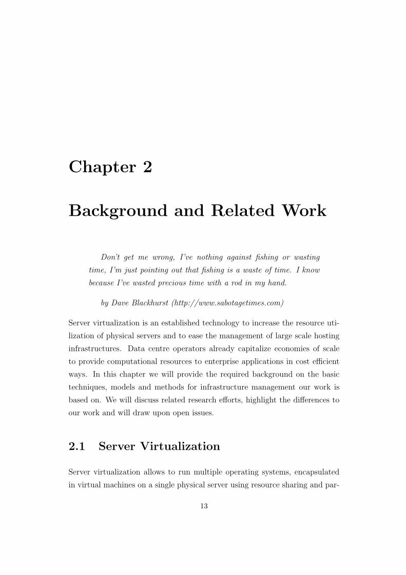
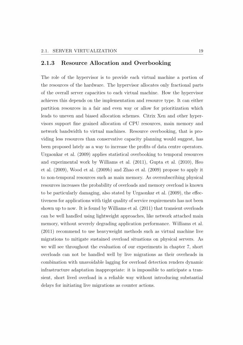
2.1 Server Virtualization
Server virtualization allows to run multiple operating systems, encapsulated
in virtual machines on a single physical server using resource sharing and par-
13
14 CHAPTER 2. BACKGROUND AND RELATED WORK
!""#$%&$'()*+,)$ -.$
CONTROL
STRATEGY
Server 1
SUT VM
SUT VM
MONITOR
ACTUATOR
SYSTEM
STATE
Hardware
SUT VM
SUT VM
Virtual Machine Monitor / Hypervisor
Virtual
Machine I
Virtual
Machine N
Management API
Virtual Hardware Interfaces
Memory Disk Network CPU
CPU Network DIsk Memory
!"!"!""
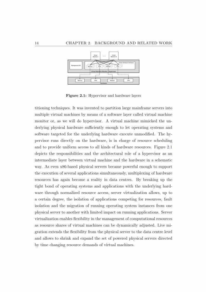
Figure 2.1: Hypervisor and hardware layers
titioning techniques. It was invented to partition large mainframe servers into
multiple virtual machines by means of a software layer called virtual machine
monitor or, as we will do hypervisor. A virtual machine mimicked the un-
derlying physical hardware sufficiently enough to let operating systems and
software targeted for the underlying hardware execute unmodified. The hy-
pervisor runs directly on the hardware, is in charge of resource scheduling
and to provide uniform access to all kinds of hardware resources. Figure 2.1
depicts the responsibilities and the architectural role of a hypervisor as an
intermediate layer between virtual machine and the hardware in a schematic
way. As even x86-based physical servers became powerful enough to support
the execution of several applications simultaneously, multiplexing of hardware
resources has again become a reality in data centres. By breaking up the
tight bond of operating systems and applications with the underlying hard-
ware through normalized resource access, server virtualization allows, up to
a certain degree, the isolation of applications competing for resources, fault
isolation and the migration of running operating system instances from one
physical server to another with limited impact on running applications. Server
virtualization enables flexibility in the management of computational resources
as resource shares of virtual machines can be dynamically adjusted. Live mi-
gration extends the flexibility from the physical server to the data centre level
and allows to shrink and expand the set of powered physical servers directed
by time changing resource demands of virtual machines.

2.1. SERVER VIRTUALIZATION 15
However, the extra layer of abstraction comes at the price of reduced appli-
cation performance as shown by Wood et al. (2008). The deviation from
native performance is often acceptable to practitioners. The overheads stem
from various tasks performed by the hypervisor such as code rewriting, trap-
ping memory access and I/O operation execution. The actual extent depends
on the type of virtualization platform and the characteristics of the hardware
architecture in use. Overheads are also incurred when executing virtual ma-
chine live migrations that depend on the employed algorithm and the memory
intensity of a virtual machine’s workload. On commodity systems, hardware
resources are heavily shared which leads to overheads caused by parallel and
shared access of virtual machines to hardware caches and memory controllers.
While overheads incurred by the virtualization layer have been studied ex-
tensively in the past, the latter issue has not received much attention in the
scientific community. We will review different types of virtualization platforms
before we discuss the mentioned overheads in more detail.
2.1.1 Types of Server Virtualization
A variety of different techniques for the implementation of virtual machines
(sometime referred to as guests) are available today. We give a short overview
of server virtualization platforms in general before we go into the details of
the Citrix Xen hypervisor developed by Citrix (2012), that we rely on in our
work. Contemporary hypervisor implementations can be classified by the way
they enable the execution of guest operating systems with and without direct
hardware access.
• Emulation and translation based platforms execute privileged guest in-
structions in software because the virtual machine’s operating system
and hardware architectures are incompatible. It allows for the execution
of unmodified operating systems but incurs the overhead of instruction
translation.
16 CHAPTER 2. BACKGROUND AND RELATED WORK
• Full virtualization platforms employ binary code translation to trap ac-
cess to non-virtualizable instructions. It allows the execution of unmodi-
fied guest operating system. VMware uses binary translation techniques
to achieve full virtualization of x86-based hardware. Hardware-assisted
virtualization enables efficient full virtualization using hardware capa-
bilities, primarily from the physical servers processors and was added
to x86 processors lately. Most modern x86-based processors support
hardware virtualization. Hardware extensions support a privilege level
beyond supervisor mode, used by the hypervisor to control the execution
of a virtual machine’s operating systems. In this way, the hypervisor can
efficiently virtualize the entire processor instruction set by handling sen-
sitive instructions using classic trap and emulate techniques implemented
in hardware.
• Paravirtualization allows the guest operating system to execute in user
mode, but provides a set of special function calls to the hypervisor, which
allows the guests to execute privileged instructions. It requires a modi-
fication of the guest operating systems to replace hardware instructions
with calls to the hypervisor.
2.1.2 Citrix Xen Virtualization Platform
Xen is an open source hypervisor for the x86 hardware platform and has been
commercialized, but is still available as an open source distribution main-
tained by Citrix. Xen introduced paravirtualization on the x86, using it to
support virtualization of modified guest operating systems without hardware
support or binary translation. Xen also allowed for full virtualization based on
hardware support and manages these hardware features using a common ab-
straction layer that enables unmodified guest operating systems to run within
Xen virtual machines. Hardware-assisted virtualization in Xen allows, through
2.1. SERVER VIRTUALIZATION 17
the addition of new instructions, paravirtualized guests to call the hypervisor
directly which allows the hypervisor to keep hardware access under control.
Above the Xen hypervisor, which runs on the highest privilege level, operate a
set of virtual machines, also called guest domains. The guests use hypervisor
services to manipulate virtual CPUs and to perform I/O operations. A special
virtual machine called domain0 owns management privileges and has direct
access to the hardware, serving as device driver domain. Domain0 can be
used to manage other virtual machines and allows them to access native device
drivers. Hardware supported virtual machines get I/O virtualization through
device emulation.
As the I/O devices are shared across all virtual machines, the hypervisor con-
trols access to them by implementing a delegation model for device access.
A split device driver design enables the execution of unmodified, native de-
vice driver in domain0. An emulated hardware interface, called the backend
driver, hides the native drivers from the guest domains. The backend driver
exposes a standardized set of hardware devices that all guest operating systems
interface with by using the front-end driver. The front-end driver communi-
cates with the backend driver via a shared-memory ring architecture and an
eventing mechanism implemented in the hypervisor. This I/O execution model
leads to additional CPU overheads in contrast to other I/O virtualization tech-
niques as it requires CPU time in domain0 and in the involved guest domain,
which requires the respective virtual CPUs to be scheduled on a physical CPU.
Liao et al. (2008) show that I/O performance depends on the employed CPU
scheduling strategy and propose modified scheduling algorithms to improve
I/O performance and to reduce CPU overhead. Cherkasova et al. (2007) pro-
vide an performance analysis of CPU scheduling in Xen. They show that both
the CPU scheduling algorithm and the scheduler parameters heavily impact
on the I/O performance.
As we will discuss in section 5.7, live migrations executed by the domain0
18 CHAPTER 2. BACKGROUND AND RELATED WORK
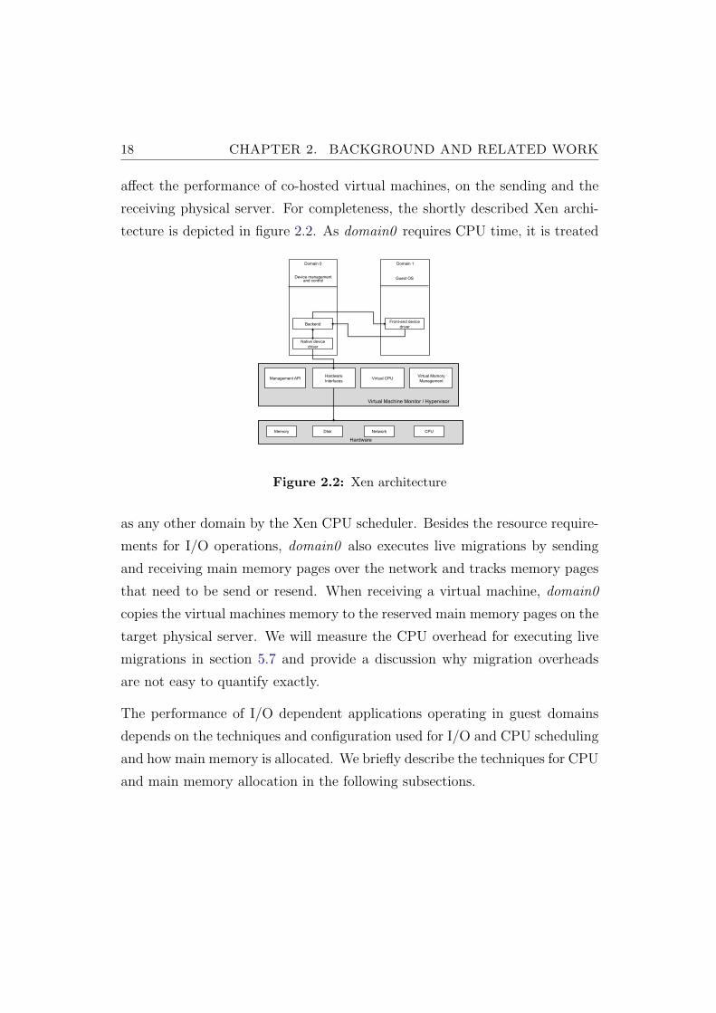
affect the performance of co-hosted virtual machines, on the sending and the
receiving physical server. For completeness, the shortly described Xen archi-
tecture is depicted in figure 2.2. As domain0 requires CPU time, it is treated
!""#$%&$'()*+,)$ -.$
Hardware
Virtual Machine Monitor / Hypervisor
Domain 0
Management API Hardware
Interfaces
Domain 1
Native device
driver
Front-end device
driver Backend
Virtual CPU Virtual Memory
Management
CPU Network DIsk Memory
Device management and control
Guest OS
Figure 2.2: Xen architecture
as any other domain by the Xen CPU scheduler. Besides the resource require-
ments for I/O operations, domain0 also executes live migrations by sending
and receiving main memory pages over the network and tracks memory pages
that need to be send or resend. When receiving a virtual machine, domain0
copies the virtual machines memory to the reserved main memory pages on the
target physical server. We will measure the CPU overhead for executing live
migrations in section 5.7 and provide a discussion why migration overheads
are not easy to quantify exactly.
The performance of I/O dependent applications operating in guest domains
depends on the techniques and configuration used for I/O and CPU scheduling
and how main memory is allocated. We briefly describe the techniques for CPU
and main memory allocation in the following subsections.
2.1. SERVER VIRTUALIZATION 19
2.1.3 Resource Allocation and Overbooking
The role of the hypervisor is to provide each virtual machine a portion of
the resources of the hardware. The hypervisor allocates only fractional parts
of the overall server capacities to each virtual machine. How the hypervisor
achieves this depends on the implementation and resource type. It can either
partition resources in a fair and even way or allow for prioritization which
leads to uneven and biased allocation schemes. Citrix Xen and other hyper-
visors support fine grained allocation of CPU resources, main memory and
network bandwidth to virtual machines. Resource overbooking, that is pro-
viding less resources than conservative capacity planning would suggest, has
been proposed lately as a way to increase the profits of data centre operators.
Urgaonkar et al. (2009) applies statistical overbooking to temporal resources
and experimental work by Williams et al. (2011), Gupta et al. (2010), Heo
et al. (2009), Wood et al. (2009b) and Zhao et al. (2009) propose to apply it
to non-temporal resources such as main memory. As oversubscribing physical
resources increases the probability of overloads and memory overload is known
to be particularly damaging, also stated by Urgaonkar et al. (2009), the effec-
tiveness for applications with tight quality of service requirements has not been
shown up to now. It is found by Williams et al. (2011) that transient overloads
can be well handled using lightweight approaches, like network attached main
memory, without severely degrading application performance. Williams et al.
(2011) recommend to use heavyweight methods such as virtual machine live
migrations to mitigate sustained overload situations on physical servers. As
we will see throughout the evaluation of our experiments in chapter 7, short
overloads can not be handled well by live migrations as their overheads in
combination with unavoidable lagging for overload detection renders dynamic
infrastructure adaptation inappropriate: it is impossible to anticipate a tran-
sient, short lived overload in a reliable way without introducing substantial
delays for initiating live migrations as counter actions.

20 CHAPTER 2. BACKGROUND AND RELATED WORK
2.1.3.1 CPU Allocation
The shared resource of main interest in the literature on workload management
in data centres is CPU time. It is allocated temporarily by a scheduler in a sim-
ilar way CPU time is scheduled to processes in modern multitasking operating
systems. There the CPU scheduler may preempt processes as required, ensures
fair allocation and aims at not wasting CPU cycles. The Xen CPU scheduler
is in charge of scheduling the virtual CPUs assigned to virtual machines on
physical CPUs. In contrast, a virtual machine’s operating system scheduler
manages operating system processes from the run queue and schedules them
on the available virtual CPUs. In Xen and other hypervisors a single virtual
machine may use one or more virtual CPUs. The scheduler is responsible to
determine which virtual CPU should be executed on which physical CPU. To
achieve the assignment task, the scheduler determines which virtual CPUs are
idle and which are busy. In a second step the scheduler selects a virtual CPU
from the busy set and assigns it to a physical CPU. A virtual CPU is idle if
no process is scheduled for execution by its operating system and is running
the idle task on a virtual CPU.
The credit based scheduler is the default algorithm in Xen. According to
Cherkasova et al. (2007), it delivers good performance for average workloads.
A cap can be used to control the CPU utilization of a virtual machine, limit-
ing it to fractions of the overall CPU capacity. A cap of zero corresponds to
the schedulers work conserving mode and allows a virtual machine to receive
spare CPU time on any physical CPU. A non-zero cap limits the amount of
CPU time a virtual machine may receive and corresponds to the non work-
conserving mode of the scheduler. The credit scheduler requires each domain
to have a weight assigned, the cap is optional. The weight indicates the rel-
ative CPU allocation a virtual machine may receive compared to co-located
virtual machines. It is a non-preemptive, fair share proportional scheduler and
supports work-conserving and non work-conserving modes using virtual ma-
2.1. SERVER VIRTUALIZATION 21
chine weights. The weights correspond to credits in a token bucket algorithm.
Credits are earned at a constant rate, saved up to a maximum, and consumed
while a virtual CPU runs on a physical CPU. Negative credits imply a priority
of over, positive balance implies a priority of under. Whenever a scheduling
decision is to be made for a physical CPU, the head of the physical CPUs run
queue is allocated to it. The run queue is sorted according to the virtual CPUs
priority. If there is no virtual CPU of priority under available in the run queue,
the queues of other physical CPUs are searched for virtual CPUs with prior-
ity under and if one is found it is scheduled. On symmetric multi-processor
hardware, system wide load balancing is achieved without explicit pinning of
virtual CPUs. Virtual machines are guaranteed to receive a fair share of CPU
time. However, Zhou et al. (2011) show how to break the guarantees and
how a virtual machine may steal CPU time from co-located virtual machines.
It is also ensured that physical CPUs only switch into the idle state if no
runnable virtual CPU are available. The basic scheduling scheme accurately
distributes resources between CPU-intensive workloads, but comes at the price
of reduced I/O performance, as shown by Liao et al. (2008). To achieve better
I/O latency, the scheduler attempts to prioritize I/O operations by boosting
priorities of virtual CPUs with left over credits waiting for I/O operations.
When a virtual CPU is awakened with remaining credits, it may exceptionally
preempt running or waiting virtual CPUs with lower priorities. That way, I/O
intensive workloads obtain low latency by requiring only occasionally small
amounts of CPU time, while the scheduler is still able to preserve a fair CPU
distribution. Knowledge of the credit scheduler is required to understand the
impact of virtual machine live migration on CPU demands on the target and
source physical server.
Several control theoretic approaches operating on very short time scales such as
seconds have been presented by Padala et al. (2007) and Padala et al. (2009),
that detect and mitigate CPU bottlenecks and provide service differentiation
by controlling CPU allocation using caps and weights. Similarly, Wood et al.
22 CHAPTER 2. BACKGROUND AND RELATED WORK
(2009a) adjusts the amount of virtual CPUs available to a virtual machine in
response to changes in demand. In contrast, we do rely on the credit based
scheduler to assign CPU time to virtual machines in a demand oriented way.
We do not control the CPU allocation as it requires knowledge of the appli-
cation running inside the virtual machine, an application may not even take
advantage of additional virtual CPUs, and we do not assume priorities for vir-
tual machines in an enterprise setting. Virtual machines are considered to be
non-discriminable in importance by the data centre control system.
2.1.3.2 Main Memory Allocation
In contrast to CPU time, main memory is often not amenable to multiplexing
or overbooking. This circumstance is often claimed to prevent higher degrees
of consolidation. Main memory is, in the parlance of Urgaonkar et al. (2009) a
non-temporal resource and requires more conservative capacity planning than
temporal resources such as CPU and network bandwidth. Even slight shortages
of main memory severely degrade application performance due to high memory
access latencies caused by page faults. The concept of overcommitting physical
memory is well studied in the context of operating systems, but much less
studied for server virtualization.
Xen allows the adaptation of main memory allocations of virtual machines, but
no automatic adjustment techniques are currently available. Virtual machines
are assigned a minimum and maximum amount of main memory that can be
adjusted using balloon drivers to temporarily remove memory from running
virtual machines. Under normal operations, every memory page of a virtual
machine is directly backed by a memory page on the physical server. The
balloon driver works by inflating or deflating a memory balloon, which is an
area of a virtual machine’s main memory address space. A balloon driver uses
an operating system specific technique to increases memory pressure within the
virtual machine. The operating system assumes that it can no longer use the
2.1. SERVER VIRTUALIZATION 23
requested memory. In response it swaps out not heavily used memory pages to
secondary storage. After acquiring memory pages, the balloon driver informs
the hypervisor that the physical memory pages that back the virtual machines
memory pages have been freed. The hypervisor in turn revokes the guest’s
access privilege to these physical memory pages, and makes them available
to other guests. When a guest’s memory allocation should be increased, the
hypervisor asks the balloon driver to deflate its memory balloon. In order
to do so, the balloon driver requests the hypervisor to remap ballooned-out
guest memory pages to physical memory pages. In case that there are no spare
physical memory pages available on the server, the hypervisor may refuse to
increase the memory allocation. After a successful increase, the swapped out
memory pages will be eventually swapped in on demand. Gupta et al. (2010)
state that as I/O operations are involved, especially in an infrastructure that
is based on network accessible storage, swapping main memory pages in and
out is an expensive operation.
Main memory overbooking has not been widely studied, except on the VMware
platform. Here, the aggregated memory allocation of all virtual machines may
exceed the memory capacity of a physical server. Waldspurger (2002) intro-
duces a technique called content-based page sharing for the VMware platform.
This technique improves the effective use of physical main memory by as much
as 33%, measured in production environments. Page sharing identifies virtual
machine memory pages with identical content and consolidates them into a
single shared page. This technique, implemented at the physical server level
applies only to virtual machine co-located on a single physical server. In a large
data centre, opportunities for content-based page sharing may only be realized
if virtual machines with similar memory contents are located on the same
physical server. Wood et al. (2009b) present a memory page sharing-aware
placement system for virtual machines. This system determines the sharing
potential among a set of virtual machines in a data centre, and computes
possibly more efficient placements. It uses live migrations to optimize virtual
24 CHAPTER 2. BACKGROUND AND RELATED WORK
machine placement in response to changes in resource demands. The evalua-
tion of the prototype, using a mix of enterprise applications, demonstrates an
increase of data center capacity by 17%, but imposes control overheads and is
specifically targeted towards the VMWare platform. The observed savings in
memory are due to fact, that applications use a limited writable working set;
a fact that is also exploited by live migration algorithms. However, it is not
stated how much of the savings are due to the fact that all virtual machines
used in the evaluation are installed using the same operating system and iden-
tical software version. Heterogeneity in deployed operating systems and appli-
cations may decrease the potential benefits noticeable. It is important to note
that changes in the degree of page sharing may lead to severe main memory
shortages on a physical server and consequently to performance degradation
for the applications running in the assigned virtual machines. These effects in
combination with volatile demands for temporal resources potentially lead to
complex interdependencies rendering the analysis of the delivered performance
of control systems difficult at best.
Amongst the few studies on dynamic memory allocation, Heo et al. (2009) use
feedback control for memory allocation in Xen. A control system prototype
for demand oriented memory allocation for virtual machines is used to show
how hosted applications achieve the desired performance in spite of their time-
varying CPU and memory demands. However, the system is evaluated in a
small scale environment without using virtual machine live migrations and
the impact on application performance to memory over-provisioning is not
shown. The applications we study in this work do not exhibit volatile memory
demand, on the contrary, their memory demands are rather stable. Memory
that is acquired once, is seldom released and instead used for enhancing caching
and buffering. Hence, in our setting, dynamic memory allocation may not lead
to substantial savings, but to rather intense levels of application performance
degradation.
Gupta et al. (2010) introduce memory sharing at finer, sub-page granularity
2.1. SERVER VIRTUALIZATION 25
that allows for higher savings of about 65%. Their technique detects duplicated
memory pages on a physical server and keeps only a single, shared copy of
that page. Milos et al. (2009) implement experimental support for memory
page sharing in Xen. However, the dynamic memory management policies in
VMWare come at substantial application performance overheads as shown by
Gupta et al. (2010). The availability of the memory balloon driver in Xen
makes it possible to dynamically repartition physical server memory among
multiple virtual machines. However, on a physical server with saturated main
memory capacity, it is only possible to increase the amount of main memory
of a single virtual machine by reclaiming the same amount of physical memory
of another virtual machine. Hence, it is only possible to run additional virtual
machines by reducing the amount of memory available to co-located virtual
machines.
Chen et al. (2010) introduce a lightweight solution to gracefully reduce the
performance degradation when memory pages need to be swapped on a phys-
ical server if page sharing and ballooning fail to revoke enough memory for
reallocation purposes. The proposed techniques prefetch pages from the phys-
ical server memory swap as long as good spatial locality in memory access
patterns persists so as to reduce disk transfers. The virtual machines are no-
tified when the hypervisor swaps out pages, which hides those pages from its
memory reclamation routines to eliminate unnecessary virtual machine swap-
ping and to prevent double paging. The experimental system shows that guest
performance can be improved substantially, but still suffers from substantial
application performance degradation.
2.1.4 Virtual Machine Live Migration
Virtual machine live migration is the process of moving a running operating
system with low impact on its availability and performance from one physi-
cal server to another. The main difficulty is to transfer the main memory and
26 CHAPTER 2. BACKGROUND AND RELATED WORK
processor state while it is constantly modified. We discuss virtual machine live
migrations in a local area network context, where physical servers are inter-
connected by high speed networks and storage systems are accessible over the
network through standard protocols like NFS or iSCSI. In a local area network,
a migrating virtual machine moves with its TCP/IP state and its IP address
by generating an unsolicited ARP request including an IP address mapping to
the MAC address of the target physical server. All receiving physical servers
and switches will update their mapping. This technique frequently reduces the
adoption time of the new MAC address to a few milliseconds. While a few
network packages in transit may be lost, very minimal impact can be expected,
especially for TCP connections. Wide area network live migrations have been
studied by Bradford et al. (2007) but also requires the migration of secondary
storage.
Currently, the live migration techniques of choice for commercial and open-
source virtualization platforms are pre-copy based approaches. In contrast,
post-copy live migration techniques have been developed but still suffer from
some severe limitations, application performance degradation ad extended pe-
riods of residual dependencies. Stop-and-copy migration (Sapuntzakis et al.,
2002) algorithms and on-demand (Zayas, 1987) migration techniques also de-
liver poor performance. The usage of the former leads to elongated service
downtimes, the latter to high total migration time, residual memory depen-
dencies and degraded application performance during the synchronization of
on-demand memory page transfers between participating physical servers.
While there has been some progress, especially for overcoming the shortcom-
ings of post-copy based algorithms (Hines et al., 2009), the currently prevailing
live migration algorithms used in Xen, Citrix or VMWare VMMotion belong
to the family of iterative pre-copy algorithms. By combining a bounded itera-
tive push phase with a final and typically short stop-and-copy phase of active
memory pages. The idea of this design relies on iterative convergence: by
iterating through multiple rounds of copying in which the virtual machines
2.1. SERVER VIRTUALIZATION 27
memory pages that have been manipulated during the previous copy phases
are resent to the destination on the assumption that at some point the num-
ber of modied pages will be small enough to stop the execution of the virtual
machines temporarily, copy the hopefully small number of remaining pages
and restart the virtual machine on the destination server. While this design
reduces both total migration time and downtime, rendering it suitable for
dynamic workload management, it incurs significant overheads on the source
and destination servers of a migration by requiring network bandwidth and
processor time.
Pre-copy based live migration algorithms aim at reducing the service down-
time a virtual machine may experience. The algorithms are based on the
key observation that only small parts, the so called writable working set of
the main memory an virtual machine is frequently modified. In pre-copy live
migration the memory allocated to a virtual machine is copied to the target
physical server in a first copy iteration. The hypervisor traps memory write
access using shadow page tables. When shadow tables are activated, the page
table of a virtual machine is replaced by an empty page table and all pages
are made read-only. The hypervisor propagates changes made to the shadow
table to the real page table forth and back. When a virtual machine modifies
its memory pages, modified pages are marked as dirty in a bitmap. The user
space migration daemon reads the bitmap to identify the memory pages that
have to be resend to the receiving physical server. After the bitmap is read,
it is cleared and all memory pages are marked as read-only again. After the
initial bulk memory transfer, a subset of the memory pages will be dirty, and
these are again send to the target physical server in a subsequent iteration.
The iterative copying goes on until the dirty memory set is sufficiently small.
Then the virtual machine is suspended at the source physical server, the re-
maining dirty memory pages are copied and the virtual machine is resumed
on the target server. Possible improvements include the exclusion of particu-
larly hot memory pages from being copied in any but the last iteration. This
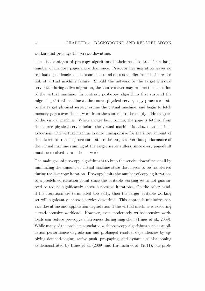
28 CHAPTER 2. BACKGROUND AND RELATED WORK
workaround prolongs the service downtime.
The disadvantages of pre-copy algorithms is their need to transfer a large
number of memory pages more than once. Pre-copy live migration leaves no
residual dependencies on the source host and does not suffer from the increased
risk of virtual machine failure. Should the network or the target physical
server fail during a live migration, the source server may resume the execution
of the virtual machine. In contrast, post-copy algorithms first suspend the
migrating virtual machine at the source physical server, copy processor state
to the target physical server, resume the virtual machine, and begin to fetch
memory pages over the network from the source into the empty address space
of the virtual machine. When a page fault occurs, the page is fetched from
the source physical server before the virtual machine is allowed to continue
execution. The virtual machine is only unresponsive for the short amount of
time taken to transfer processor state to the target server, but performance of
the virtual machine running at the target server suffers, since every page-fault
must be resolved across the network.
The main goal of pre-copy algorithms is to keep the service downtime small by
minimizing the amount of virtual machine state that needs to be transferred
during the last copy iteration. Pre-copy limits the number of copying iterations
to a predefined iteration count since the writable working set is not guaran-
teed to reduce significantly across successive iterations. On the other hand,
if the iterations are terminated too early, then the larger writable working
set will signicantly increase service downtime. This approach minimizes ser-
vice downtime and application degradation if the virtual machine is executing
a read-intensive workload. However, even moderately write-intensive work-
loads can reduce pre-copys effetiveness during migration (Hines et al., 2009).
While many of the problem associated with post-copy algorithms such as appli-
cation performance degradation and prolonged residual dependencies by ap-
plying demand-paging, active push, pre-paging, and dynamic self-ballooning
as demonstrated by Hines et al. (2009) and Hirofuchi et al. (2011), one prob-
2.2. RESOURCE ALLOCATION ON MULTI-CORE CHIPS 29
lem with post copy migration is that a failure of the network or the source
or destination host during migration, will result in irrecoverable failure of the
migrating virtual machine, because no physical server possesses a current and
complete version of the virtual machines execution state.
Xen uses a tailored pre-copy algorithm that is executed in domain0. The algo-
rithm requires the use of memory shadow page tables to keep track of dirtied
memory pages, which in turn requires the hypervisor to trap each main mem-
ory write access. The migration daemon needs to access the virtual machines
main memory and copies memory pages over the network interfaces at the
maximum bandwidth rate available, which saturates the network link for the
duration of a migration.
2.2 Resource Allocation on Multi-Core Chips
During the consolidation planning process, the additional resource require-
ments for virtualization and server consolidation need to be taken into con-
sideration. While modern multiprocessor servers provide abundant hardware
parallelism to achieve server consolidation, contention for available processing
cores, hardware caches and memory bandwidth may introduce performance
isolation concerns and additional resource demands. Hence, an estimate of the
effects of resource contention and virtualization overheads need to be included
into the consolidation planning method.
Despite advantages such as security and fault isolation, current virtualization
techniques do not provide effective performance isolation between virtual ma-
chines (Koh et al., 2007). Specifically, contention for physical resources impacts
performance to varying degrees in different workload configurations, causing
significant variance in observed system throughput and response times. The
contention effects will be even more prevalent on multi-core processors, as their
30 CHAPTER 2. BACKGROUND AND RELATED WORK
use has become prevalent in data centres and multi-core systems are very likely
to be equipped with even more cores per chip in the future.
For scheduling algorithms used on multi-core systems, the primary goal for
placing threads on cores is load balancing. Operating system schedulers try
to balance the runnable threads across the available cores to ensure fair dis-
tribution of CPU time and minimize the idling of cores. However, there is
a fundamental aw with this strategy which arises from the fact that a core
is not an independent processor but rather a part of a larger on-chip system
and hence shares resources with other cores. It has been documented by Tam
et al. (2009) that the execution time of a thread can vary greatly depending
on which threads run on the other cores of the same chip. This is especially
true if several cores share the same last-level cache or if several threads share
a single core thereby sharing the whole cache hierarchy.
There exists a certain body of work that explores the performance degrada-
tion applications incur when running in isolation on virtualized servers, or how
different virtual machines affect each other when running on a physical server
(Huber et al. (2011), Wood et al. (2008), Menon et al. (2005), Gupta et al.
(2006), Pu et al. (2010), Koh et al. (2007)). However, a limited amount of stud-
ies exist that address the issue of resource overheads incurred by contention
for shared hardware resources, that lead to non additive resource demands of
virtual machines. The main body of work on static server consolidation as-
sumes additivity for resource demands of multiple virtual machines running
simultaneously on a physical server. However, this assumption does not hold
true on commodity hardware. Operating multiple virtual machines hosting en-
terprise workloads simultaneously introduces contention for shared resources
on a physical server with non-dedicated hardware components as shown by
Iyer et al. (2009). By utilizing a measurement approach based on a bench-
mark for server consolidation it is shown how hardware metrics such as cycles
per instruction and cache misses per instruction increase through shared cache
space and memory bandwidth contention. It is found that contention for pro-
2.3. STATIC SERVER CONSOLIDATION 31
cessing cores reduces processor utilization while contention for shared cache
space increases the required cycles per instruction and consequently measured
CPU utilization. In their experiments, they show an increase of over 40% in
required cycles per instruction due to the consolidation of virtual machines on
a multi-core physical server. Their findings are derived using a consolidation
benchmark that employs typical enterprise applications. The main source for
increased CPU utilization is attributed to shared last level cache interference
effects. Cache sensitive applications are shown to cause CPU utilization to
increase even if only a small fraction of the last level cache is not exclusively
usable. While Blagodurov et al. (2010) also find that cache contention does
have an effect on performance degradation, it is not the only source for con-
tention. As the cache miss rate is highly correlated with contention for other
shared resources (e.g. if two threads share a cache which causes excessive cache
misses, the threads will also compete for resource on all memory hierarchy lev-
els between the shared cache and the main memory of the physical server) it is
found to be a well suited predictor for contention effects. This insights extends
up the path to first level caches if two threads run on a single core in parallel.
In contrast to several works on contention effects, the findings in Iyer et al.
(2009) are of most relevance to our work as the workloads employed resemble
the ones we are interested in. Most other works are based on micro-benchmark
suited to identify shortcomings in cache-sharing and access strategies, but do
not influence much on solving practical overhead estimation problems.
2.3 Static Server Consolidation
Static server consolidation is the process of allocating virtual machines to
physical servers with the aim to minimize the amount of required physical
servers. The task requires careful resource demand estimation even under
highly stochastic, time dependent resource demand behavior to ensure suffi-
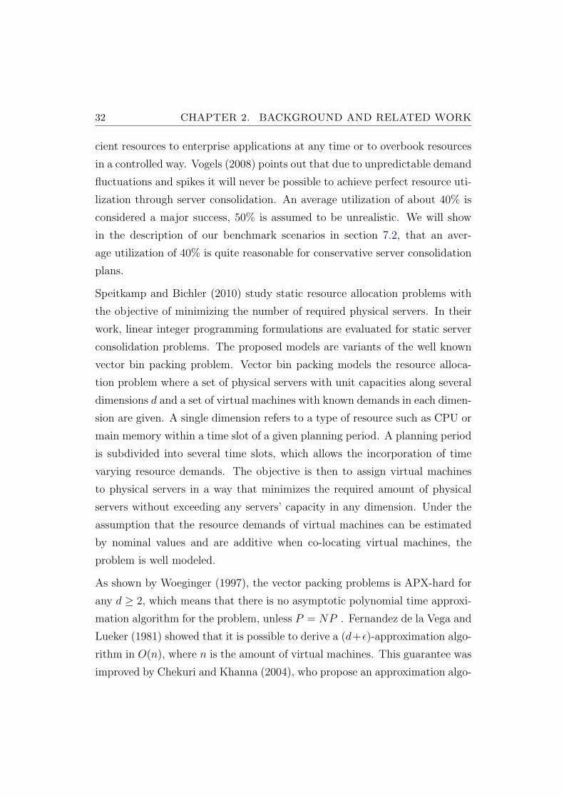
32 CHAPTER 2. BACKGROUND AND RELATED WORK
cient resources to enterprise applications at any time or to overbook resources
in a controlled way. Vogels (2008) points out that due to unpredictable demand
fluctuations and spikes it will never be possible to achieve perfect resource uti-
lization through server consolidation. An average utilization of about 40% is
considered a major success, 50% is assumed to be unrealistic. We will show
in the description of our benchmark scenarios in section 7.2, that an aver-
age utilization of 40% is quite reasonable for conservative server consolidation
plans.
Speitkamp and Bichler (2010) study static resource allocation problems with
the objective of minimizing the number of required physical servers. In their
work, linear integer programming formulations are evaluated for static server
consolidation problems. The proposed models are variants of the well known
vector bin packing problem. Vector bin packing models the resource alloca-
tion problem where a set of physical servers with unit capacities along several
dimensions d and a set of virtual machines with known demands in each dimen-
sion are given. A single dimension refers to a type of resource such as CPU or
main memory within a time slot of a given planning period. A planning period
is subdivided into several time slots, which allows the incorporation of time
varying resource demands. The objective is then to assign virtual machines
to physical servers in a way that minimizes the required amount of physical
servers without exceeding any servers’ capacity in any dimension. Under the
assumption that the resource demands of virtual machines can be estimated
by nominal values and are additive when co-locating virtual machines, the
problem is well modeled.
As shown by Woeginger (1997), the vector packing problems is APX-hard for
any d ≥ 2, which means that there is no asymptotic polynomial time approxi-
mation algorithm for the problem, unless P = NP . Fernandez de la Vega and
Lueker (1981) showed that it is possible to derive a (d+ε)-approximation algo-
rithm in O(n), where n is the amount of virtual machines. This guarantee was
improved by Chekuri and Khanna (2004), who propose an approximation algo-
2.3. STATIC SERVER CONSOLIDATION 33
rithm with a (1+dε+ ln(1ε)) worst case guarantee. More recently, Bansal et al.
(2009) gave a rather complex algorithm with a 1 + ln(d) guarantee. However,
both algorithms have exponential runtime requirements in d or even worse. For
large values of d, the guarantee is rather loose and given the runtime require-
ments of limited practical relevance. Yao (1980) showed that no algorithm
with running in time O(n log(n)) can give better than a d-approximation.
Despite the rather discouraging approximation results, Speitkamp and Bichler
(2010) show that theoretically hard problems can be solved for modest sized
real world instances and that simple approximation algorithms derived from
the well know any-fit family often produced highly competitive, if not opti-
mal solutions. Approximation algorithms belonging to the any-fit family for
the vector bin packing problem have already been studied decades ago in a
numeric way by Maruyama et al. (1977). Their worst-case behavior has been
studied by Kou and Markowsky (1977) and Csirik et al. (1990), their average
behavior over practical instances by Maruyama et al. (1977) and Roy et al.
(2008) in the context of distributed real-time embedded systems. The results
indicate that the existing performance guarantees are quite pessimistic for real
world problems. Approximation algorithms beyond the standard greedy ones
are proposed by Leinberger et al. (1999) and Maruyama et al. (1977).
In contrast, the classical bin packing problem, where each item is determined
by a single, nominal value, is very well studied and tight approximation guar-
antees for the first-fit decreasing algorithm have been given by Johnson and
Garey (1985) exist. Even though lately, Dosa (2007) improved the worst case
bound by giving a tight bound of the additive constant in the guarantee (the
constant was decreased from 1 to 69), the bin packing problem can be consid-
ered well studied and can be solved well with existing, simple approximation
algorithms.
As of today, even static consolidation approaches as introduced by Urgaonkar
et al. (2009) and Rolia et al. (2004) that employ stochastic workload models
rely on the efficiency of approximation algorithms. The low computational

34 CHAPTER 2. BACKGROUND AND RELATED WORK
complexity have already been utilized by dynamic workload management in
data centers due to real time requirements for making virtual machine place-
ment decisions. It is also known that commercial products for static consoli-
dation employ simple approximation algorithms as the size of typical problems
consisting of several hundreds or even thousands of virtual machines renders
exact algorithms impractical.
The stochastic packing problem, where resource demands are defined by ran-
dom variables rather than nominal point estimates, has been studied by Klein-
berg et al. (2000) in the context of network bandwidth allocation. The authors
study statistical multiplexing from the perspective of approximation algo-
rithms with a focus on on-off demand source that can be modeled as Bernoulli
trials. The authors derive performance bounds for polynomial time algorithms
for this type of stochastic demand and extend their investigation to distribu-
tions that specify the probability p of high demand values that are given as
a nominal value. It is shown that there exist a polynomial time algorithm
that has a O(log(p−1) log(n)) worst case deviation guarantee from the optimal
solution.
Stillwell et al. (2010) propose a new formulation of the multi-resource allocation
problem in shared hosting platforms for static server consolidation that aims
at application performance, fairness, and increased server utilization. Several
classes of resource allocation algorithms are proposed for the problem as well
as the classical vector bin packing problem, which are evaluated in numeric
simulations using artificial data. Their work identifies an approximation al-
gorithm that achieves average performance close to the optimal across many
experimental scenarios. Furthermore, the algorithm exposes moderate run-
time for large problem instances and thus is usable in practice. The scope of
their work is static consolidation where the number of virtual machines and
the resource demands of virtual machines do not change throughout time. It
is noted that in practice resource allocations for virtual machines need to be
adapted throughout time. The proposed algorithms can be used to recompute
2.4. DYNAMIC WORKLOAD MANAGEMENT 35
appropriate resource allocations periodically or based on particular events.
The authors state the need for a planning approach that is aware of over-
heads for virtual machine reassignments. Without including these overheads,
a newly computed allocation could be widely different from the previous one,
possibly leading to unnecessary and excessive migrations. One solution is to
compute resource allocations that are likely to delay the need for allocation
adaptation as much as possible, as proposed by Ali et al. (2008). Another,
complementary option is to adapt the resource allocation while minimize the
amount of change required as proposed by Karve et al. (2006). The mentioned
work strives dynamic workload management that, due to real time constraints,
requires the use of approximation algorithms developed in the context of static
server consolidation.
2.4 Dynamic Workload Management
Dynamic workload management and fine grained resource access control has
been mainly driven by application level performance objectives, as done by
Wang et al. (2009), Zhang et al. (2007) Appleby et al. (2001), Urgaonkar et al.
(2008) and Abdelzaher et al. (2002). In contrast, Verma et al. (2008) addresses
the problem of power and migration cost aware virtual machine placement in
heterogeneous server clusters. The work investigates on the viability of us-
ing CPU utilization based, application specific power consumption models to
develop virtual machine placement algorithms and validates the proposed sys-
tem using an experimental data centre infrastructure using a limited set of
experiments. Similar to this work, Kumar et al. (2010) propose a system that
also aims at minimizing virtual machine migrations that are often triggered
by largely fluctuating resource demands. The proposed method embraces un-
predictable short term fluctuations through stochastic demand modeling and
is able to reduce the amount of required virtual machine live migrations by
36 CHAPTER 2. BACKGROUND AND RELATED WORK
a factor of two in contrast to existing virtual machine placements methods.
However, again the evaluation is conducted on a very limited set of workload
traces and the influence of system control parameters such as thresholds is
not investigated upon. Their work shows that power consumption on a single
physical server can be reduced by about 10 % by optimally placing virtual
machines in response to changes in their CPU demands. It is not shown how
much energy can be saved by completely evacuating physical servers nor is an
estimate given how many live migrations might be needed by a clairvoyant,
optimal control strategy. Whether the achieved energy consumption reduc-
tions as well as the reduction in live migrations are significant or close to what
could be achieved is left unanswered.
A main motivation for our study of reactive control systems is the existence
of commercial systems that rely on reactive methods that derive ad-hoc live
migration and virtual machine placement decisions. For example, VMwares
Distributed Resource Scheduler (VMWare, 2012a) uses live migrations for au-
tomated load balancing in response to resource shortages or extended periods
of underutilization. It monitors virtual machine resource demands in a black-
box way, without taking application specific information into consideration as
done by Wood et al. (2009a).
One of the earliest work in the area of dynamic workload management that
does not rely on virtualization, but on using dedicated physical server is given
by Chase et al. (2001). The proposed resource management architecture is
designed to save energy. By operating an active set of servers at predefined
utilization thresholds and by sending lightly utilized servers servers to low
power consumption states, the system adapts to dynamically changing work-
loads. The system continuously monitors utilization levels and plans resource
assignments by estimating the effects on application performance. Experimen-
tal results from a prototype show that the system adapts to changes in the
applied workload and can reduce server energy usage by 29% or more for typ-
ical web application workloads in contrast to using a static pool of physical
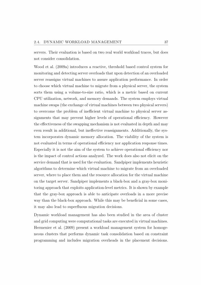
2.4. DYNAMIC WORKLOAD MANAGEMENT 37
servers. Their evaluation is based on two real world workload traces, but does
not consider consolidation.
Wood et al. (2009a) introduces a reactive, threshold based control system for
monitoring and detecting server overloads that upon detection of an overloaded
server reassigns virtual machines to assure application performance. In order
to choose which virtual machine to migrate from a physical server, the system
sorts them using a volume-to-size ratio, which is a metric based on current
CPU utilization, network, and memory demands. The system employs virtual
machine swaps (the exchange of virtual machines between two physical servers)
to overcome the problem of inefficient virtual machine to physical server as-
signments that may prevent higher levels of operational efficiency. However
the effectiveness of the swapping mechanism is not evaluated in depth and may
even result in additional, but ineffective reassignments. Additionally, the sys-
tem incorporates dynamic memory allocation. The viability of the system is
not evaluated in terms of operational efficiency nor application response times.
Especially it is not the aim of the system to achieve operational efficiency nor
is the impact of control actions analyzed. The work does also not elicit on the
service demand that is used for the evaluation. Sandpiper implements heuristic
algorithms to determine which virtual machine to migrate from an overloaded
server, where to place them and the resource allocation for the virtual machine
on the target server. Sandpiper implements a black-box and a gray-box moni-
toring approach that exploits application-level metrics. It is shown by example
that the gray-box approach is able to anticipate overloads in a more precise
way than the black-box approach. While this may be beneficial in some cases,
it may also lead to superfluous migration decisions.
Dynamic workload management has also been studied in the area of cluster
and grid computing were computational tasks are executed in virtual machines.
Hermenier et al. (2009) present a workload management system for homoge-
neous clusters that performs dynamic task consolidation based on constraint
programming and includes migration overheads in the placement decisions.
38 CHAPTER 2. BACKGROUND AND RELATED WORK
The use of constraint programming allows the system to determine near op-
timal virtual machine to physical server assignments and outperforms assign-
ments based on simple approximation algorithms. As migration overhead is
taken into account when deriving assignment decisions, migrations are chosen
that can be implemented efficiently, incurring a low performance overhead.
The authors notice that large migration overheads may nullify the benefits of
dynamic workload management.
Dhiman et al. (2010) introduce a system that manages power consumption in
consolidated infrastructures and reassigns virtual machine with the objective
to reduce the power consumption on all physical servers and aims at reducing
the overall active set of physical servers at any point in time. The system
estimates the relationship between the architectural characteristics of a vir-
tual machine, its performance and power consumption. Based on the learned
application performance and power profile of the hosted virtual machines, the
system aims at intelligently placing virtual machine on physical servers. The
system does not deal with time varying resource demands but characterizes
workloads based on steady state demands, exercising micro benchmark appli-
cations. Their system is able to reduce the overall energy consumption by
about 20% compared to existing virtual machine scheduling and placement
algorithms.
A large body of work that is close to ours is based on simulation studies.
Khanna et al. (2006) proposed a dynamic workload management algorithm,
which is triggered when a physical server becomes overloaded or under-loaded.
The main goals of their algorithm are to guarantee service level conformance,
to minimize live migration cost and the required number of physical servers
used at any point in time. Their approach is reactive and threshold based and
is shown to work well in simulations of real workload traces. A similar method
is proposed in Bobroff et al. (2007) that also considers service level agreements.
The main contribution is the evaluation of a dynamic workload management
algorithm to reduce the amount of required capacity and the amount of service
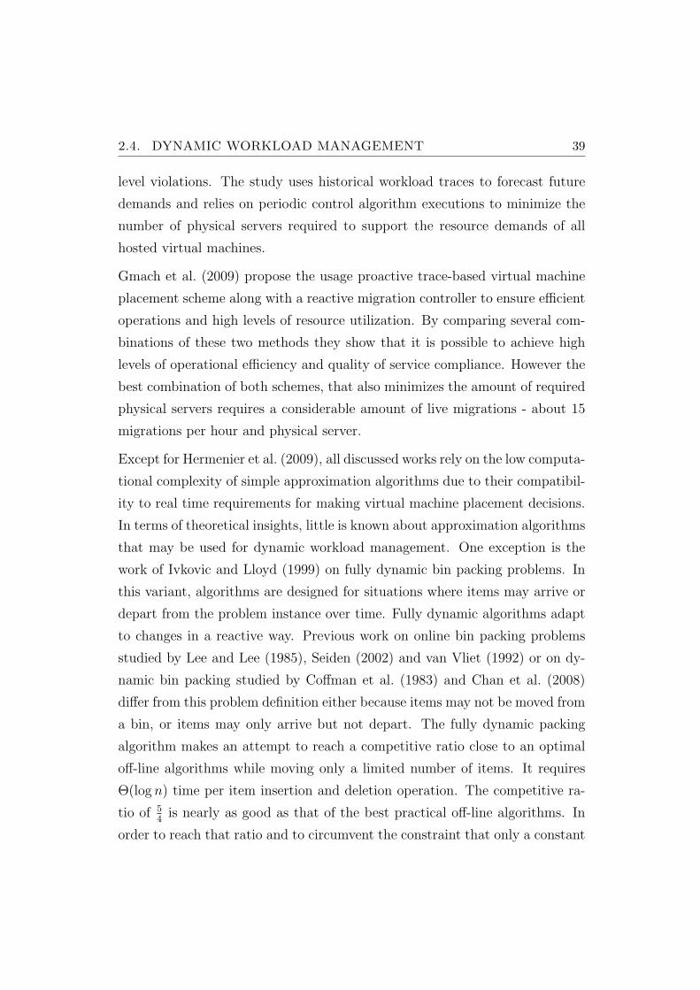
2.4. DYNAMIC WORKLOAD MANAGEMENT 39
level violations. The study uses historical workload traces to forecast future
demands and relies on periodic control algorithm executions to minimize the
number of physical servers required to support the resource demands of all
hosted virtual machines.
Gmach et al. (2009) propose the usage proactive trace-based virtual machine
placement scheme along with a reactive migration controller to ensure efficient
operations and high levels of resource utilization. By comparing several com-
binations of these two methods they show that it is possible to achieve high
levels of operational efficiency and quality of service compliance. However the
best combination of both schemes, that also minimizes the amount of required
physical servers requires a considerable amount of live migrations - about 15
migrations per hour and physical server.
Except for Hermenier et al. (2009), all discussed works rely on the low computa-
tional complexity of simple approximation algorithms due to their compatibil-
ity to real time requirements for making virtual machine placement decisions.
In terms of theoretical insights, little is known about approximation algorithms
that may be used for dynamic workload management. One exception is the
work of Ivkovic and Lloyd (1999) on fully dynamic bin packing problems. In
this variant, algorithms are designed for situations where items may arrive or
depart from the problem instance over time. Fully dynamic algorithms adapt
to changes in a reactive way. Previous work on online bin packing problems
studied by Lee and Lee (1985), Seiden (2002) and van Vliet (1992) or on dy-
namic bin packing studied by Coffman et al. (1983) and Chan et al. (2008)
differ from this problem definition either because items may not be moved from
a bin, or items may only arrive but not depart. The fully dynamic packing
algorithm makes an attempt to reach a competitive ratio close to an optimal
off-line algorithms while moving only a limited number of items. It requires
Θ(log n) time per item insertion and deletion operation. The competitive ra-
tio of 54
is nearly as good as that of the best practical off-line algorithms. In
order to reach that ratio and to circumvent the constraint that only a constant

40 CHAPTER 2. BACKGROUND AND RELATED WORK
number of items may be moved, the algorithm bundles very small items and
treats them as a single larger item. While the algorithm is designed to move
smaller items in favor of large items, it is not aiming at minimizing migration
overhead as required in a practical setting. Without bundling small items into
a single larger item when moves are required, it may even lead to an excessive
amount of single movements.
Chapter 3
Problem and Model Definitions
If I had an hour to solve a problem and my life depended on the
solution, I would spend the first 55 minutes determining the proper
question to ask, for once I know the proper question, I could solve
the problem in less than five minutes.
by Albert Einstein
In this chapter we introduce the basic resource allocation problem and intro-
duce some required notation and vocabulary. We assume the role of a data
centre operator hosting a set of virtual machines, J on a set of identical phys-
ical servers I. The virtual machines are managed by a hypervisor operating
on the physical servers. Each virtual machine j ∈ J is running an enterprise
application stack or a subset of the tiers of a multi-tiered application. We dis-
tinguish virtual machines by their type g(j). The type of a virtual machine is
determined by the application tier it is running. We restrict our study to three
types of virtual machines: (1) virtual machines running all tiers, subsequently
referred to as monolithic application configuration, (2) virtual machines run-
ning a web and application server and (3) virtual machines running a database
41
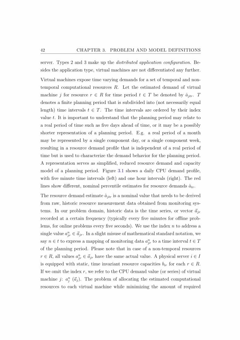
42 CHAPTER 3. PROBLEM AND MODEL DEFINITIONS
server. Types 2 and 3 make up the distributed application configuration. Be-
sides the application type, virtual machines are not differentiated any further.
Virtual machines expose time varying demands for a set of temporal and non-
temporal computational resources R. Let the estimated demand of virtual
machine j for resource r ∈ R for time period t ∈ T be denoted by ajtr. T
denotes a finite planning period that is subdivided into (not necessarily equal
length) time intervals t ∈ T . The time intervals are ordered by their index
value t. It is important to understand that the planning period may relate to
a real period of time such as five days ahead of time, or it may be a possibly
shorter representation of a planning period. E.g. a real period of a month
may be represented by a single component day, or a single component week,
resulting in a resource demand profile that is independent of a real period of
time but is used to characterize the demand behavior for the planning period.
A representation serves as simplified, reduced resource demand and capacity
model of a planning period. Figure 3.1 shows a daily CPU demand profile,
with five minute time intervals (left) and one hour intervals (right). The red
lines show different, nominal percentile estimates for resource demands atr.
The resource demand estimate ajtr is a nominal value that needs to be derived
from raw, historic resource measurement data obtained from monitoring sys-
tems. In our problem domain, historic data is the time series, or vector ~ajr
recorded at a certain frequency (typically every five minutes for offline prob-
lems, for online problems every five seconds). We use the index n to address a
single value anjr ∈ ~ajr. In a slight misuse of mathematical standard notation, we
say n ∈ t to express a mapping of monitoring data anjr to a time interval t ∈ Tof the planning period. Please note that in case of a non-temporal resources
r ∈ R, all values anjr ∈ ~ajr have the same actual value. A physical server i ∈ Iis equipped with static, time invariant resource capacities bir for each r ∈ R.
If we omit the index r, we refer to the CPU demand value (or series) of virtual
machine j: anj (~aj). The problem of allocating the estimated computational
resources to each virtual machine while minimizing the amount of required
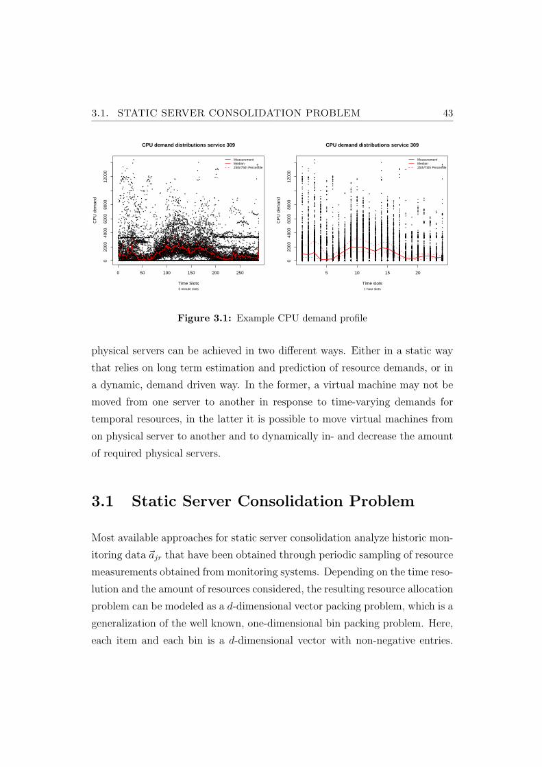
3.1. STATIC SERVER CONSOLIDATION PROBLEM 43
●●
●
●
●
●
●
●
●
●
●
●
●●
●
●
●●
●
●
●
●
●
●
●
●
●
●
●
●
●
●
●
●●
●
●
●
●●
●
●
●
●
●
●
●
●
●
●
●
●
●
●
●
●
●
●
●
●
●
●
●
●
●
●
●
●
●
●
●
●
●
●
●
●
●
●
●
●
●
●
●
●
●●●
●
●
●
●
●
●
●●
●
●
●
●
●
●
●
●
●
●
●
●
●●
●
●
●
●
●
●
●
●
●
●
●
●
●
●
●
●
●
●
●
●
●
●
●
●
●●
●
●
●
●●●
●●
●
●
●●●
●●●
●
●
●
●
●
●
●
●
●
●
●
●
●
●
●
●
●
●
●
●
●●
●
●
●
●
●
●
●
●
●
●
●
●
●
●
●
●
●●
●
●
●
●
●
●
●
●
●
●
●
●
●●
●
●
●
●
●
●
●
●
●
●
●
●
●
●
●
●
●
●
●
●
●
●
●
●
●
●
●
●
●●
●
●
●
●
●
●
●
●
●●●
●
●
●●
●
●
●
●
●
●
●
●
●●
●●
●
●
●
●
●
●
●
●
●
●
●
●
●
●
●
●
●
●
●
●
●
●
●
●
●
●●
●
●
●●
●
●
●
●
●
●
●
●
●
●
●●
●
●
●
●
●
●
●
●●●
●●
●
●
●
●
●●
●
●
●
●
●
●
●
●
●
●
●
●
●
●
●
●
●
●
●
●●
●
●●
●
●
●
●
●
●
●●
●
●
●
●●
●
●●
●●
●
●
●●●
●
●
●
●
●
●●
●
●
●
●
●
●
●
●
●
●
●
●
●●
●
●
●
●●
●
●
●
●
●●
●
●
●●
●
●
●
●
●
●
●
●
●
●
●
●
●
●
●
●
●●●●
●
●
●
●
●
●
●
●
●●
●
●
●
●
●
●
●
●●
●
●●
●
●
●
●
●
●
●
●●
●
●
●
●●
●
●
●
●
●
●
●
●●●
●
●
●●
●
●
●●●
●
●
●
●
●●
●
●
●
●
●
●
●
●
●
●
●
●
●●
●
●
●
●
●
●
●
●
●
●
●
●
●
●●
●
●
●
●
●
●●
●
●
●
●
●
●
●
●●
●
●●
●
●
●
●
●
●●
●
●
●
●
●
●
●
●
●
●
●
●
●
●
●
●●
●
●●
●
●
●
●
●
●
●●
●
●
●
●
●
●
●
●
●
●
●
●
●
●
●
●
●
●●●
●
●
●
●
●
●
●
●
●
●
●
●
●
●
●
●
●
●
●
●●●
●
●
●
●
●
●
●●
●
●
●
●
●
●●
●
●
●
●
●
●
●
●
●
●
●
●
●●
●
●
●●
●
●
●
●
●
●
●
●
●
●
●
●
●
●
●
●
●
●
●
●●●
●
●
●
●
●
●
●
●
●
●
●
●
●
●
●
●
●
●
●
●
●●
●
●
●
●●
●
●
●
●
●●
●
●
●
●
●
●
●
●
●
●
●
●
●
●
●
●
●
●
●
●
●
●●
●
●
●
●
●
●
●
●
●
●●
●●
●
●
●
●
●
●
●
●
●●
●
●
●
●●
●
●
●●
●
●
●
●
●
●●
●
●
●
●
●
●
●
●
●
●
●
●
●●
●●
●
●
●●●
●
●●
●
●
●
●●
●
●
●
●
●
●●
●
●●
●
●
●
●
●
●
●
●●
●
●
●
●
●
●
●
●
●
●
●
●
●
●
●
●
●
●
●
●
●
●
●
●
●
●
●●
●
●●
●
●
●
●●
●
●●
●●●
●
●
●
●
●
●
●
●
●●
●
●●●
●
●
●
●
●
●
●
●
●●
●
●
●
●
●
●
●
●
●●●
●
●
●
●
●●●●
●
●
●
●
●●
●●●●
●
●
●
●
●
●
●●
●●
●
●
●
●●●●
●
●
●
●
●
●
●
●●
●
●
●
●
●
●
●
●
●
●●
●
●
●
●
●
●
●
●
●
●
●
●
●
●
●
●
●
●●●●●
●
●●
●
●
●
●
●●
●●●●
●
●
●
●●●
●
●
●
●
●
●
●
●
●
●
●
●
●
●
●
●
●●
●●
●
●●
●
●
●
●
●
●
●
●
●●
●
●
●
●
●
●
●
●
●
●
●
●
●●●●
●
●
●
●
●
●
●
●
●
●
●
●
●
●
●
●
●
●
●●●
●
●
●●●
●
●●
●
●
●
●
●
●●
●
●
●
●
●
●
●
●
●
●
●
●
●
●
●
●●●●
●
●
●
●
●●
●
●
●
●●
●
●
●
●
●
●
●
●
●
●
●
●
●
●
●
●
●
●
●
●
●
●
●
●
●
●
●
●
●
●
●
●
●
●
●
●
●●
●
●
●●●●●
●
●
●●
●
●
●
●
●
●
●
●
●
●
●
●
●
●●
●
●
●
●
●
●
●
●
●
●
●
●
●
●
●
●●
●
●
●
●
●
●●
●
●
●
●
●
●
●
●●●●●
●
●
●
●
●
●
●
●
●
●
●
●
●
●
●
●
●
●●
●
●
●
●
●●
●
●
●
●●
●
●
●
●
●
●
●
●
●
●
●
●
●
●
●
●
●●
●
●
●●
●
●●
●
●
●
●
●
●
●
●●
●
●
●
●●
●●
●
●●●
●
●
●
●
●
●
●
●
●●
●
●
●
●
●
●
●
●
●●
●
●
●
●
●
●
●
●●●●●
●
●●
●
●
●●
●
●
●
●●
●
●
●
●
●
●
●
●
●
●
●
●
●
●
●
●
●
●
●
●
●●
●
●
●
●
●
●
●
●
●
●
●
●
●
●
●
●
●●●
●●●●●
●
●
●●
●
●
●
●
●
●
●
●
●
●
●
●
●
●
●
●
●
●
●
●
●
●●
●●
●
●
●
●
●
●
●
●
●
●
●
●
●
●
●
●
●
●
●
●●
●●●●
●
●
●
●●
●
●
●
●
●
●
●
●
●
●
●
●
●
●
●●
●
●
●
●
●
●●●
●
●
●
●
●
●
●
●
●
●
●●
●
●
●
●
●
●
●
●
●
●
●●
●
●
●
●
●
●
●
●
●
●
●
●
●
●
●
●
●
●
●
●
●
●
●
●
●
●
●
●
●
●
●●
●
●
●
●
●
●
●
●
●
●
●
●
●
●
●
●●
●
●
●●
●●
●
●
●
●
●
●●
●
●
●
●
●
●
●
●
●
●
●●
●
●
●
●
●
●
●
●
●
●
●
●
●
●
●
●
●
●
●
●
●
●
●
●
●
●
●
●
●
●
●●●●
●●●●
●
●
●
●●
●
●
●
●
●
●
●
●
●
●
●
●
●
●
●
●●
●
●
●
●
●
●
●●
●
●
●
●
●
●
●
●
●●
●
●
●
●
●
●
●
●
●
●●
●●●●●
●
●
●●
●
●
●
●
●
●
●
●
●
●
●
●
●
●
●
●●
●
●
●
●
●●
●
●
●
●
●
●
●
●
●●
●
●
●
●
●
●
●
●
●
●
●●●
●●●●●
●
●
●
●
●
●
●
●
●
●
●
●
●
●
●
●
●
●●
●
●
●
●
●
●
●
●
●
●
●
●
●
●
●
●
●
●
●
●●
●
●●
●
●
●
●
●●●●●●●●
●
●
●
●
●
●
●
●
●
●
●
●
●
●
●
●
●
●
●
●
●
●
●
●
●
●
●
●
●
●
●
●●
●
●
●
●●
●
●
●
●
●
●
●
●
●
●●●●●●●●
●
●
●
●
●
●
●
●
●
●
●
●
●
●
●
●
●
●
●●
●
●
●
●
●
●
●
●
●
●
●
●
●
●
●
●
●
●
●
●
●
●
●
●
●
●
●
●●●●●●●●
●
●
●
●
●
●
●
●
●●●
●
●
●
●
●
●
●
●
●●
●
●
●
●
●
●
●
●
●
●
●
●
●
●
●
●
●
●
●
●
●
●●
●
●
●
●●●●●●●●
●
●
●
●●
●
●
●
●●
●
●
●
●
●
●
●
●
●
●
●
●
●
●●
●
●
●
●
●
●
●
●
●
●
●
●
●
●
●
●
●
●●
●
●
●
●●●●●●●●
●
●
●
●
●
●
●●
●●
●●
●
●
●
●
●
●
●
●
●
●
●
●
●
●
●
●
●
●
●
●●
●
●
●
●
●
●
●
●
●●
●
●
●
●
●●●
●●●●●
●
●
●
●
●
●
●
●
●
●
●●
●
●
●
●
●
●
●
●
●
●
●
●
●
●
●
●●
●
●
●
●
●
●
●
●
●
●
●
●
●●
●
●
●
●
●
●●
●●●●●
●
●
●
●
●
●
●
●
●
●
●●
●
●●
●
●
●
●
●
●
●
●
●●
●
●
●
●
●
●
●●
●
●
●
●
●
●
●
●
●
●●
●
●
●●●●
●●●●●
●
●
●
●
●
●
●
●
●●●
●
●
●●
●
●●●
●
●
●
●
●●
●
●●
●●
●
●
●
●
●
●
●
●
●
●
●
●
●
●
●
●
●●●●
●●●●●
●
●
●
●
●
●
●
●
●●●●
●
●
●
●
●●●
●
●
●
●
●●
●
●
●●●
●
●
●
●
●
●
●
●
●
●
●
●
●
●●
●
●●●●
●●●●●
●
●
●
●
●
●
●
●
●●●
●
●
●
●
●
●●●
●
●
●
●
●●
●
●
●●●
●
●
●
●
●
●
●
●
●
●
●
●
●
●●
●
●●●●
●●●●●
●
●
●
●
●
●
●
●
●●●●
●
●
●
●
●●●●
●
●
●
●●
●
●●●●
●
●●
●
●
●
●
●●●
●
●
●●●
●
●●●●●●●●●
●
●
●
●
●
●
●
●
●●●●
●
●●
●
●●●●
●
●
●
●●
●
●●●●
●
●
●
●
●
●
●
●●
●
●
●
●●●
●
●●●
●●●●●●
●
●
●
●
●
●
●
●●●
●
●
●
●●
●
●
●
●●
●
●
●
●●
●
●●●●
●
●●
●
●
●
●●●
●
●
●
●●●
●
●●●●●●
●●
●
●
●
●
●
●
●
●●
●
●
●
●
●
●●
●
●
●
●
●
●
●
●
●●
●
●●●
●
●
●
●●
●
●
●●●●
●
●
●●●
●
●●●●●●●●●
●
●
●
●
●
●
●
●
●
●
●
●
●
●●
●
●
●
●●
●
●●●●
●
●●●●
●
●
●●
●
●
●●●●
●
●
●●●
●
●●●●●●●●●
●
●
●
●
●
●
●
●
●
●●●
●
●●
●
●●●
●
●
●●●●
●
●●●●
●
●
●
●
●
●
●●●
●
●
●
●●
●
●
●●●●●●●●●
●
●
●
●
●
●
●
●●
●
●●
●
●
●
●
●●●
●
●
●●●●
●
●●●
●
●
●
●
●
●
●
●●●●
●
●
●
●●
●
●
●●●
●●
●
●●
●
●
●
●
●
●
●
●
●
●
●●
●
●
●
●
●●●●
●
●●●●
●
●●●
●
●
●
●
●
●
●
●●
●
●
●
●●●●
●
●
●
●●
●●●●●
●
●
●
●
●
●
●
●
●
●●●
●
●●
●
●●●●
●
●●●●
●
●
●●●
●
●
●●
●
●
●●●●
●
●
●●●
●
●●●●●●●●●
●
●
●
●
●
●
●
●
●
●
●●
●●●
●
●
●●●
●
●●●
●
●
●
●
●●
●
●●
●
●
●
●●
●
●
●
●
●●●
●
●●●●
●●●●●
●
●
●
●
●
●
●
●
●
●
●●●
●●
●
●●●●
●
●●●●
●
●●●●
●
●●
●
●
●
●●●●
●
●
●●●
●
●●●●●●
●
●●
●
●
●
●
●
●
●
●
●
●
●●
●
●●
●
●●●●
●
●●●●
●
●●●●
●
●●
●
●
●
●●●●
●
●
●●●
●
●
●●●●●
●
●●
●
●
●
●
●
●
●
●
●
●
●●
●
●●
●
●●●●
●
●●●●
●
●●●●
●
●●
●
●
●
●●●●
●
●
●●●
●
●
●●●●●
●
●●
●●
●
●
●
●
●
●
●
●
●●
●
●●
●
●●●●
●
●
●
●●
●
●●●●
●
●●
●
●
●
●●●●
●
●
●●●
●
●●●●
●●
●
●●
●●
●
●
●
●
●●
●
●
●●
●
●●
●
●●●●
●
●●●●
●
●
●●●
●
●●
●
●
●
●●●●
●
●
●●●
●
●
●●●●●
●
●●
●●
●
●
●
●
●
●●
●
●●
●
●
●
●
●●●●
●
●●●●
●
●●●
●
●
●●
●
●
●
●●●●
●
●
●●●
●
●●●●●●
●
●●
●●
●
●
●
●
●
●
●
●●●
●
●●
●
●
●
●●
●
●●●●
●
●●●●
●
●●
●
●
●
●●●●
●
●●●●
●
●●●
●
●●
●
●●
●●
●
●
●
●
●
●
●
●●●
●
●●
●
●
●
●●●●●●●
●
●●●●
●
●●
●
●
●
●●●●
●
●●●●
●
●●●●●●
●
●●
●
●
●
●
●
●
●
●
●
●
●●
●●●
●
●
●
●●
●●●●●
●
●●●
●
●
●
●●
●
●
●●
●
●
●
●
●
●●
●
●●
●●
●●
●
●●
●
●
●
●
●
●
●●
●
●
●
●
●
●
●
●●●●●
●
●●●●
●
●●●●
●
●●●
●
●
●
●●
●
●
●
●●
●
●
●
●
●●
●●
●
●●
●●
●
●
●
●
●●
●
●
●
●
●
●●
●●
●
●●
●
●●●●
●
●●●●
●
●●●
●
●
●●●●●●●●●
●
●●●●
●●
●
●●
●
●
●
●
●
●
●
●
●
●
●
●●
●●
●
●
●
●●
●
●●
●●●●●
●●
●
●●●●
●
●●●●●
●
●●●
●
●●●
●
●●
●
●●●
●
●
●
●
●
●
●●
●
●
●●●●
●
●●●●
●
●●●●●●
●●●
●
●
●●
●
●
●●
●●●
●
●●●
●
●●●●●●
●
●●
●
●
●
●
●
●
●
●●
●
●
●
●
●●
●
●●
●●
●
●●●●●
●
●●●
●
●
●●●
●
●●●●●
●
●●●
●
●●●●●●
●
●●
●
●
●
●●
●
●●
●
●
●
●
●
●●
●
●●
●●●●●●●●●●●●
●
●●●●
●
●●
●●
●
●
●●●
●
●
●
●
●
●●
●●●
●
●
●
●
●
●
●
●
●
●
●
●
●
●●
●
●●●
●
●
●
●
●
●●●●●
●
●
●●
●
●
●●
●
●●
●
●●●●
●
●●●
●
●●
●
●
●
●●
●
●
●
●
●
●
●
●
●
●●●●
●
●●●
●●●●
●
●
●●
●●
●●
●●
●
●●
●
●
●●●●●●●
●●
●●
●
●●
●
●
●
●
●
●
●
●
●
●
●
●
●
●
●●●
●
●
●●
●
●●●
●
●●●
●●●
●
●
●
●
●
●
●
●
●
●
●●●●●●
●
●●
●●
●●
●
●●
●
●
●
●
●
●
●
●●
●
●
●
●
●
●
●
●
●
●
●
●
●
●
●●
●
●●●
●
●
●
●●●
●
●
●●●●
●
●●
●
●
●
●●●
●●
●
●●
●
●
●
●
●
●
●
●
●
●
●
●●
●
●
●
●
●●●
●
●
●
●
●
●
●
●
●
●
●
●
●
●
●
●
●●●
●
●
●
●●
●
●
●
●●●
●●
●
●
●
●
●●
●●
●
●
●
●
●
●
●
●
●
●
●
●●●
●
●
●
●
●●
●
●●
●●
●
●
●
●
●
●
●●●
●
●
●
●
●●
●
●
●
●●
●●
●●
●
●
●●
●
●
●
●
●
●
●
●
●
●
●
●
●
●●●●
●
●
●●●
●
●
●●
●
●
●
●
●
●
●
●
●
●
●
●
●●●
●
●
●●
●
●●●
●
●
●
●
●
●
●
●
●
●
●
●●
●
●●
●
●
●
●
●
●
●
●
●●●●
●
●
●
●
●●
●
●
●
●
●
●●●●
●
●
●
●●
●
●●
●●
●●
●
●
●
●
●
●
●
●
●
●●●
●
●
●
●
●
●●
●
●
●
●
●
●●●
●
●
●
●●
●
●
●
●
●
●
●
●
●
●
●
●
●
●
●
●
●
●
●
●
●
●●
●
●
●
●
●
●
●
●
●
●
●
●
●
●
●
●
●
●
●
●
●
●
●
●
●
●
●●
●
●
●●
●
●
●
●
●
●
●
●
●
●
●
●
●
●
●
●●
●●
●
●
●●
●
●
●
●
●
●
●
●
●
●
●
●
●
●
●
●
●
●
●
●
●
●
●
●
●
●
●
●
●
●
●
●
●
●
●
●
●
●
●
●
●
●
●
●
●
●
●
●
●
●
●
●
●
●●
●
●
●
●
●
●
●
●
●
●
●
●
●
●●
●
●
●
●
●
●
●
●
●
●
●
●
●
●
●
●
●
●
●
●
●
●
●
●
●
●
●
●
●
●
●●
●
●
●
●
●
●
●●
●
●●
●
●
●
●
●
●
●
●
●
●
●●
●
●
●
●
●
●
●
●
●
●
●
●
●
●
●
●
●
●
●
●
●
●
●
●
●
●
●●
●
●
●
●●
●
●
●
●
●
●●
●
●
●
●
●
●
●
●
●
●●
●
●
●
●●
●
●
●
●
●
●
●
●
●
●
●
●
●
●
●
●
●
●
●●
●
●
●
●
●
●
●
●
●
●●
●
●
●
●
●
●
●●
●
●
●
●
●
●
●
●
●
●
●
●
●
●●
●
●
●
●
●
●
●
●
●
●
●
●
●
●
●
●
●
●
●
●
●
●
●
●
●
●
●
●
●
●
●
●
●
●
●
●
●
●
●●
●
●
●
●
●
●
●
●
●
●●
●
●
●
●
●
●
●
●
●
●
●
●
●
●
●
●●
●
●
●
●
●●
●
●
●
●
●
●
●
●●
●
●
●
●
●
●
●
●●
●
●●
●
●
●
●
●
●
●
●
●
●●
●
●
●
●
●
●
●
●
●
●
●
●
●
●
●
●
●
●
●
●●
●●
●
●●
●●
●
●●
●
●
●
●●
●
●
●
●
●
●
●●
●
●
●
●
●
●
●
●
●
●
●
●
●
●
●
●
●
●
●
●
●
●
●
●
●●
●●
●
●
●
●
●
●
●
●
●
●
●
●
●
●
●
●
●
●
●
●
●
●
●●
●
●●
●
●
●
●
●
●
●
●
●
●
●
●
●
●
●
●
●
●
●
●
●
●
●
●
●
●
●●
●
●
●
●●
●
●
●
●
●●
●
●
●
●
●
●
●
●
●
●
●
●
●●
●●
●
●
●
●
●
●
●
●
●
●
●
●
●
●●
●●●
●
●●
●
●
●●
●
●
●
●
●●
●
●
●
●
●
●
●
●
●
●
●
●
●●
●
●
●
●
●●
●
●
●●
●
●
●
●
●
●
●
●
●
●
●
●
●
●
●
●
●●
●
●
●
●
●
●
●
●●
●
●
●
●
●
●
●
●
●
●
●
●
●
●
●
●
●●
●
●
●
●
●
●●
●
●●
●●
●
●
●
●
●
●
●
●
●
●
●
●
●
●
●
●
●
●
●
●
●
●●
●
●
●
●
●
●
●
●
●
●
●
●
●
●
●
●
●
●
●●
●●
●
●
●
●
●
●
●●
●
●
●
●
●
●
●
●
●
●
●
●
●
●
●
●●
●
●
●
●
●
●
●
●
●●
●
●
●
●
●
●
●
●
●
●
●
●
●
●
●
●
●
●
●
●
●
●
●
●
●
●
●●
●
●
●
●
●
●
●
●
●
●
●
●
●
●
●
●
●
●
●
●
●
●
●
●
●●
●
●
●●
●
●
●
●
●
●
●
●
●
●
●
●
●
●
●
●●
●
●
●
●
●
●
●●
●
●
●
●
●
●●
●
●
●
●
●
●
●
●
●
●
●
●
●
●
●
●
●
●
●
●
●
●
●
●
●●
●
●
●
●
●
●
●
●
●
●
●
●
●
●
●
●
●
●
●
●
●●
●●
●
●
●
●
●
●
●
●●
●
●
●
●
●
●
●
●
●●
●
●
●
●
●
●
●
●
●
●
●
●
●
●
●
●
●
●
●
●
●
●
●
●
●
●
●
●
●
●
●
●
●●
●
●
●
●
●
●
●
●
●
●
●
●
●
●
●
●
●●
●
●
●
●
●
●
●
●
●
●
●
●
●
●
●
●
●
●
●
●
●
●
●
●
●
●
●
●
●
●
●
●
●
●
●
●●
●
●
●
●
●
●
●
●
●
●
●
●
●
●
●
●
●
●
●●
●
●
●
●
●
●●
●
●
●●
●●●
●●
●
●
●●
●
●
●
●●
●
●
●
●
●
●
●
●
●●
●
●
●
●
●
●
●
●
●
●
●
●
●
●
●
●
●
●
●
●
●
●
●
●
●
●
●
●
●
●
●●
●
●
●
●
●
●
●
●
●
●
●
●
●
●
●
●
●
●●
●
●
●●
●
●
●
●
●
●
●
●
●
●
●
●
●●
●
●
●
●
●
●
●●
●
●
●
●
●
●
●
●
●
●
●
●
●
●
●
●
●
●
●
●
●
●
●
●
●
●
●
●
●
●
●
●●
●
●
●
●
●
●
●
●
●
●
●
●
●●
●
●
●
●
●
●
●
●
●
●
●
●
●
●
●
●●
●
●
●
●
●
●
●
●
●
●
●
●●
●
●
●
●
●
●
●
●
●
●●
●
●
●
●
●
●
●
●●
●
●
●
●
●
●
●
●
●
●
●
●
●
●●
●
●
●
●
●
●
●
●
●
●
●
●
●
●
●
●
●
●●
●●
●
●
●
●
●
●
●
●
●●
●
●
●
●
●
●●
●
●
●
●
●
●
●
●
●
●
●
●
●
●
●
●
●
●
●
●
●
●
●
●
●
●
●
●●
●
●
●
●
●
●
●
●●
●
●
●
●
●
●
●
●
●●
●
●
●
●
●
●
●
●
●
●
●
●
●
●
●
●
●
●
●
●●
●
●
●
●
●
●
●
●
●
●
●
●
●
●
●
●
●
●
●
●
●
●
●
●
●
●
●●
●
●
●
●
●●
●
●
●
●
●
●
●
●
●
●
●
●
●
●
●
●
●
●
●
●
●
●
●
●
●
●
●
●
●
●
●
●●
●
●
●
●
●
●
●
●
●
●
●
●●
●
●
●
●
●
●
●
●●
●
●
●
●
●
●
●●●
●
●
●
●
●
●
●
●
●●●
●
●●
●
●
●
●
●
●
●
●
●
●●
●
●
●
●
●
●●
●●
●
●
●
●
●
●
●
●
●
●
●●
●
●
●
●
●
●
●
●
●
●
●
●
●●
●
●
●
●
●●
●●
●
●
●
●
●
●
●
●
●
●
●
●
●
●
●
●
●
●
●
●
●
●
●
●
●
●
●
●
●
●
●
●●
●
●
●
●
●
●
●
●
●
●
●
●
●
●
●
●
●
●
●
●
●
●
●
●
●●
●
●
●
●●
●
●
●
●
●
●
●
●
●
●
●
●
●
●
●
●
●
●
●
●
●
●
●●
●
●
●
●
●
●
●
●
●
●
●
●
●
●
●
●
●
●
●
●
●
●●
●
●
●
●●●
●
●
●●
●
●
●
●
●
●
●
●
●
●
●
●
●
●
●
●
●
●
●
●
●●
●
●
●
●
●
●
●
●
●
●
●
●
●
●
●
●
●
●
●
●
●
●
●
●
●
●
●
●
●
●
●
●
●
●
●
●
●
●
●
●
●
●
●
●
●
●
●
●
●
●
●
●
●
●●
●
●
●
●
●
●
●
●
●
●
●
●
●
●
●
●
●
●
●
●
●
●●
●
●
●
●
●●
●
●
●
●
●
●
●
●
●
●
●
●
●
●
●
●
●
●
●
●
●
●
●
●
●●
●
●
●
●
●
●
●●
●
●
●
●
●
●
●
●
●
●
●
●
●
●●
●
●
●
●
●
●
●
●
●
●
●
●
●
●
●
●
●
●
●
●
●
●
●
●●●
●
●
●
●
●●
●
●
●
●
●
●
●●
●
●
●
●
●
●
●
●
●
●
●●●
●
●
●
●
●
●●
●
●
●
●
●
●
●
●
●●
●
●
●
●
●
●
●
●
●●
●
●
●
●
●
●●
●
●
●
●
●
●
●
●
●
●
●
●
●
●
●
●
●
●
●
●
●
●●
●●
●
●
●●
●
●●
●
●
●
●
●
●
●
●
●
●
●
●
●
●
●
●
●
●
●
●●
●●
●
●
●
●
●
●
●
●
●
●
●
●
●
●
●
●
●
●
●
●
●
●
●
●
●●
●
●●
●
●
●
●
●
●
●
●
●
●
●●
●
●
●
●
●
●
●
●
●
●
●
●
●●
●
●
●
●
●
●
●
●
●
●
●
●
●
●
●
●
●
●
●
●
●
●
●
●
●
●
●
●
●
●
●
●
●
●
●●
●
●●●
●
●
●
●
●
●
●
●
●
●
●
●
●
●●
●
●
●
●
●
●
●
●
●
●
●
●●
●
●
●
●
●
●
●
●
●
●
●
●
●
●
●
●
●
●
●●
●
●
●
●
●
●
●
●
●
●
●
●
●
●
●
●
●
●
●
●
●●
●
●
●
●
●●
●
●
●
●
●
●
●
●
●
●
●
●
●
●
●
●
●
●
●●
●
●
●
●
●
●
●
●●
●
●
●
●
●
●
●
●
●
●
●
●●
●
●
●
●
●
●●
●
●
●
●
●
●
●
●
●
●
●●
●
●
●
●
●
●
●
●
●
●
●
●
●
●
●
●
●
●
●
●
●
●
●
●
●●
●
●
●●
●
●
●
●
●
●
●
●
●
●
●
●●
●
●
●
●
●
●
●
●
●
●
●
●
●
●
●
●●
●
●
●
●
●
●
●
●●
●
●
●
●
●
●
●
●
●
●
●
●
●
●●
●
●
●
●
●
●
●●
●
●
●●
●●
●
●
●
●
●●
●
●
●
●
●
●
●
●
●
●
●
●
●
●
●
●
●
●
●
●
●
●
●
●
●
●
●
●
●
●
●
●
●
●
●
●
●
●
●
●
●
●
●
●
●
●
●
●●
●
●
●
●
●
●
●
●
●
●
●●
●
●
●
●
●●
●
●●●
●
●
●
●
●
●
●
●
●
●
●
●
●
●
●●
●
●
●
●
●
●
●
●
●
●
●
●
●
●
●
●●
●
●
●
●
●
●
●
●
●
●
●
●
●
●
●
●
●
●
●
●
●
●
●
●
●
●
●
●
●
●
●
●
●
●●
●
●
●●
●
●
●
●
●
●
●
●
●
●
●
●
●
●
●●
●
●
●
●
●
●
●
●
●
●
●
●
●
●
●
●
●
●
●
●
●
●
●
●
●
●
●
●●
●
●
●
●
●
●
●
●
●
●
●
●●
●
●
●
●
●
●●
●
●
●
●
●●
●
●
●
●
●
●
●
●
●
●
●
●
●
●
●
●
●
●
●
●
●
●
●
●
●
●
●
●
●
●
●
●●
●
●●
●
●
●
●
●
●●
●
●
●
●
●●
●
●
●
●
●●
●
●
●
●
●
●
●
●
●
●
●●
●
●
●
●
●●
●
●
●
●
●
●
●
●
●
●
●
●●
●
●
●
●
●
●
●
●
●
●
●●
●
●
●
●
●
●
●
●
●
●
●●
●
●
●
●
●
●
●
●
●
●
●
●
●
●
●
●
●
●
●
●●
●
●
●
●
●
●
●
●
●
●
●
●
●
●
●
●
●
●
●
●
●
●
●
●
●
●
●
●
●
●
●
●
●●
●
●●
●
●
●
●
●
●
●
●
●
●
●●
●
●
●
●
●
●
●
●
●●
●●
●
●
●
●
●
●
●
●
●
●
●
●
●
●
●
●
●
●
●
●
●
●
●
●
●
●
●●
●
●
●
●
●
●
●
●
●
●
●
●
●
●
●
●
●
●
●
●
●
●
●
●
●
●
●
●
●
●
●
●
●
●
●
●
●
●
●
●
●
●
●
●
●
●
●
●
●
●
●
●
●
●●
●
●
●
●
●
●
●●
●
●
●
●●
●
●
●
●
●
●
●
●
●
●
●
●
●
●
●
●
●
●
●
●
●
●
●
●
●
●
●
●
●
●
●
●
●
●
●
●
●
●
●
●
●●
●
●
●
●
●
●
●
●
●
●
●
●
●
●
●
●
●
●
●
●
●
●
●●
●
●
●
●
●
●
●
●
●
●
●●
●
●
●
●
●
●
●
●
●
●
●●
●
●
●
●
●
●●
●
●
●
●
●
●
●
●
●
●
●
●●
●
●
●
●
●
●
●
●
●
●
●
●
●
●
●
●
●
●
●
●
●
●
●
●
●
●
●
●
●
●
●
●
●
●
●
●
●
●
●
●
●●
●
●
●
●
●
●
●
●
●●
●
●
●
●
●
●
●
●
●●
●
●
●
●
●
●
●
●
●●
●
●
●
●●
●
●
●
●
●
●
●
●
●
●
●
●
●
●
●
●
●
●
●●
●
●
●
●
●
●
●●
●
●
●
●
●
●
●
●
●
●
●
●
●
●
●
●
●●
●
●●
●
●●
●
●
●
●
●●
●
●
●
●
●
●
●
●
●
●●
●
●
●
●
●●
●
●
●
●
●
●
●
●
●
●
●
●
●
●
●
●
●
●
●
●
●●
●
●
●
●
●
●
●
●●
●
●
●
●
●
●
●
●
●
●
●
●
●
●
●
●
●
●●
●
●
●
●●
●
●
●
●
●
●
●
●
●
●
●
●
●
●
●
●
●
●
●
●
●
●●
●
●
●
●
●
●
●●●
●
●
●
●
●
●
●
●
●
●
●
●
●
●
●
●
●
●
●●
●
●●
●
●
●
●
●
●
●
●
●
●
●
●
●
●
●
●
●
●
●
●
●
●
●
●
●
●
●
●
●
●
●
●
●
●
●
●
●
●●
●
●
●
●
●
●
●
●
●●
●●
●
●
●●
●
●
●
●
●
●
●
●
●
●
●
●
●
●
●
●
●
●
●
●
●
●
●
●
●
●
●
●
●
●
●
●
●●
●
●
●
●
●
●
●
●
●
●
●
●
●
●
●
●
●
●
●
●●
●
●
●
●
●
●
●
●
●
●
●
●
●
●
●
●
●
●
●
●
●
●
●
●
●
●
●
●●
●
●
●
●
●
●
●
●
●
●
●●
●
●
●
●
●
●
●
●
●
●
●
●
●●
●
●
●
●
●
●
●
●
●
●
●
●
●
●
●
●
●
●
●
●
●
●
●
●
●
●
●
●
●
●
●
●
●
●
●
●
●
●
●
●
●
●
●
●
●
●
●
●
●
●
●
●
●
●
●
●
●
●
●
●
●
●
●
●
●
●
●
●
●
●
●
●
●
●
●●
●
●
●
●●●
●
●●
●
●●
●
●
●
●
●
●
●
●
●
●
●
●
●
●●
●
●
●
●
●
●●
●
●
●
●
●
●
●
●
●
●
●
●
●
●
●
●
●
●
●
●●
●
●
●●
●
●
●
●●
●
●
●
●
●●
●
●
●
●
●
●
●
●
●
●
●
●
●
●
●
●
●
●●
●
●
●
●
●
●
●
●
●
●
●
●●
●
●
●
●
●
●
●
●●
●
●
●●
●
●
●
●
●
●
●
●
●
●
●
●
●
●
●
●
●
●
●
●
●
●
●●
●
●●
●
●
●
●
●
●
●
●
●
●
●
●
●
●
●
●
●
●
●
●
●
●
●
●
●
●
●
●
●
●
●
●
●
●
●●
●
●
●
●
●
●
●
●
●
●
●
●
●
●
●●
●
●●
●
●
●
●
●
●
●
●
●
●
●
●
●
●
●
●
●
●
●
●
●
●
●
●
●●
●
●
●
●
●
●
●
●
●
●
●
●
●
●
●
●
●
●
●
●
●
●
●
●
●●
●
●
●
●
●
●
●
●
●
●
●
●
●
●
●
●
●
●
●
●
●
●
●
●
●
●●
●
●
●
●
●
●
●
●
●
●
●
●
●
●
●
●
●
●
●
●
●
●
●
●
●
●
●
●●
●
●
●
●
●
●
●
●
●
●
●
●
●
●
●
●
●
●
●
●
●
●
●
●
●●
●
●
●
●
●
●●●
●
●
●
●
●●
●
●
●
●
●
●
●
●
●
●
●
●●
●
●
●
●
●
●
●
●
●
●
●
●●
●
●
●
●
●
●
●
●
●
●
●
●
●
●
●
●
●
●
●
●●
●
●
●
●
●
●●
●
●
●
●
●
●
●
●
●
●
●
●
●
●
●
●
●
●
●
●
●
●
●
●
●
●
●●
●
●
●
●
●
●
●
●
●
●
●
●
●
●
●
●
●
●
●
●
●
●
●
●
●
●
●
●
●●
●
●●
●
●
●
●
●●
●
●
●
●
●
●
●
●
●
●
●
●
●
●
●
●
●
●●
●
●
●
●
●
●
●
●
●●
●
●●
●
●●
●
●
●
●
●
●
●●
●
●
●
●
●
●
●
●
●
●
●
●
●
●
●
●
●
●
●
●
●
●
●
●
●
●
●
●
●
●
●●
●
●
●
●
●
●●
●
●
●
●
●●
●
●●●
●
●
●●
●
●
●
●
●
●
●
●
●
●
●
●●
●
●
●●●
●
●
●
●
●
●
●
●
●
●
●
●
●
●
●
●
●
●
●
●
●
●
●
●
●
●
●
●
●
●
●●●
●
●
●
●
●
●
●
●
●
●
●
●
●
●
●
●
●
●
●
●●
●
●
●
●
●
●
●
●
●
●
●
●
●
●
●
●●
●
●
●
●
●
●
●
●
●
●
●
●
●
●
●●
●
●
●
●
●
●
●●●
●
●
●
●
●
●
●
●
●
●●
●●
●
●
●
●
●
●
●
●
●
●
●
●
●
●
●
●
●
●
●
●
●
●
●
●
●
●●
●
●
●
●
●
●●●
●
●●
●
●
●
●
●
●●
●
●
●
●●
●
●
●
●
●●
●
●
●
●
●
●
●
●
●
●
●
●
●
●
●
●
●
●
●
●
●
●
●
●
●
●●
●●
●
●
●
●
●
●
●
●
●
●
●
●
●
●
●
●
●
●
●
●
●●●
●
●
●
●
●
●
●
●
●
●
●
●
●
●
●
●
●●
●
●
●
●
●
●
●
●
●
●●
●
●
●
●
●
●
●
●
●
●
●
●
●
●
●
●
●
●
●
●
●
●
●
●
●
●
●
●●
●
●
●
●
●
●
●
●
●●
●
●
●
●
●
●
●
●
●
●
●●
●
●
●
●
●
●
●
●
●
●
●
●
●
●
●
●
●
●
●
●
●
●
●
●
●
●
●
●
●●
●
●
●
●
●
●
●
●
●
●
●
●
●
●
●
●
●
●
●●
●
●
●
●●
●
●
●
●
●
●●
●
●
●●
●
●
●
●
●●
●
●
●
●
●●
●
●
●●
●
●
●
●
●
●
●
●
●
●●
●
●
●
●
●
●
●
●
●●●
●
●
●
●
●
●●
●
●●
●
●
●
●
●
●
●
●
●
●
●
●●
●
●
●
●
●
●
●
●
●
●
●
●
●
●●
●
●
●
●
●
●
●
●
●
●
●●
●
●
●
●
●
●
●
●
●●
●
●
●
●
●●
●
●
●
●
●
●
●
●
●●
●
●
●
●
●
●
●●
●
●
●
●
●
●
●
●
●
●
●
●
●
●
●
●
●
●
●
●
●
●
●
●●
●
●
●
●
●
●
●
●
●
●
●
●
●
●
●
●
●
●●
●
●
●
●
●
●
●
●
●
●
●
●
●
●
●
●
●
●
●
●
●
●
●
●
●
●
●●
●
●●
●
●
●
●
●
●
●
●
●
●
●
●
●
●
●
●
●
●
●
●
●
●
●
●
●
●
●
●
●
●
●
●
●
●
●●
●
●
●
●
●
●
●
●
●
●
●
●●
●
●
●
●
●
●
●
●
●
●
●
●
●
●
●
●
●
●
●
●
●
●
●
●
●
●
●
●
●
●
●
●
●
●
●
●
●●
●
●
●
●
●
●
●●
●
●●
●
●
●
●
●●
●
●
●
●
●
●
●
●
●
●
●
●
●
●
●
●
●
●
●
●
●
●
●
●
●
●
●
●
●
●
●
●
●
●●
●
●
●●
●
●
●
●
●
●
●
●●
●
●
●
●
●
●●
●
●
●
●
●
●
●
●
●
●●
●●
●
●
●
●
●
●●
●
●
●
●●
●
●
●
●
●
●
●
●●
●
●●
●
●
●
●
●
●
●
●
●
●
●
●
●
●
●
●
●●
●
●
●
●
●
●
●
●
●
●
●
●
●
●
●
●
●
●
●
●
●
●
●
●
●
●
●
●
●
●
●
●
●
●
●
●
●
●
●
●
●
●
●
●
●
●
●
●
●●
●
●
●
●●
●
●
●
●
●
●
●
●
●
●
●
●
●
●
●
●
●
●
●
●
●
●
●
●
●
●
●
●
●
●
●
●
●
●
●
●
●
●
●
●
●
●
●
●
●
●
●
●
●
●
●
●
●
●●
●
●
●
●
●
●
●
●
●
●
●
●
●
●
●
●
●
●
●●
●●●
●
●
●
●
●
●
●
●
●
●
●●
●
●
●
●
●●
●
●
●
●
●
●
●
●
●
●
●
●
●●
●
●
●
●
●
●
●
●
●
●●●
●
●
●
●
●
●
●
●
●
●
●
●
●
●
●
●
●
●
●
●
●
●
●
●
●
●●
●
●●
●
●
●
●
●
●
●
●
●
●
●
●●
●
●
●
●
●
●
●
●
●
●●
●
●
●
●
●
●
●
●
●
●
●
●
●
●
●
●
●
●
●
●
●●
●
●
●
●
●
●
●●●
●
●
●
●●
●
●
●
●
●
●
●●
●
●
●
●
●
●
●
●
●
●
●
●
●
●
●
●
●
●
●
●
●
●●
●
●
●
●
●
●
●
●
●
●
●
●
●
●●●●
●
●
●
●
●
●
●
●
●
●
●
●
●
●●
●
●
●
●
●
●
●
●
●
●
●
●
●
●
●
●
●
●
●
●
●
●
●
●
●
●
●
●
●
●
●
●
●
●
●
●
●
●
●
●
●
●
●
●
●
●
●
●
●
●
●
●
●
●●
●
●
●
●
●
●
●
●
●
●
●
●
●
●
●
●
●
●
●
●
●
●
●
●
●
●
●
●
●
●●
●
●
●
●
●
●
●
●
●
●
●
●
●
●
●
●
●
●●
●
●
●
●
●
●
●
●
●
●
●
●
●
●
●
●
●
●
●
●
●
●
●
●
●
●
●
●●
●●
●
●
●
●
●
●
●
●
●
●
●
●
●
●●
●
●
●
●
●
●
●
●
●
●
●
●
●●
●
●
●
●
●
●
●
●
●
●
●
●
●
●
●
●
●
●
●
●●
●
●
●
●●
●
●
●
●
●
●
●
●
●
●
●
●
●
●
●
●
●
●
●
●
●
●
●
●
●
●
●
●●
●
●
●
●
●
●
●
●
●
●
●
●
●
●
●
●
●
●
●
●●
●
●
●
●
●
●
●
●●
●
●
●
●●
●●
●
●
●
●
●
●
●
●
●●
●
●
●
●
●
●
●●
●
●
●
●
●
●
●
●
●
●
●
●
●
●
●
●
●
●
●
●
●
●
●
●
●
●
●
●
●
●
●
●
●
●
●
●
●
●
●
●
●●
●
●●
●
●
●
●
●
●
●
●
●●
●●
●
●
●
●
●
●
●
●
●
●
●
●
●
●
●
●
●
●●
●
●
●
●
●
●
●
●
●
●
●
●
●
●
●
●
●
●
●
●
●
●
●●
●
●
●
●
●
●
●
●
●●
●
●
●
●
●
●
●
●
●
●●
●
●
●
●
●
●
●
●
●
●
●
●
●
●
●
●
●
●
●
●
●●
●●
●
●
●
●
●
●●
●
●●
●
●
●
●
●
●
●
●
●●
●
●
●
●
●
●
●
●
●
●●
●
●
●
●
●
●
●
●
●
●
●
●
●
●
●
●
●
●
●
●
●
●
●
●
●
●
●
●
●
●
●
●●
●
●
●
●
●
●
●
●
●
●●
●
●
●●
●
●
●
●
●
●
●
●
●
●
●
●
●
●
●
●
●
●
●
●
●
●
●
●●
●
●
●
●
●
●
●
●
●
●
●
●
●
●
●
●
●
●
●●
●
●
●
●
●
●
●
●
●
●
●
●
●
●
●
●
●
●
●
●
●
●
●
●
●
●
●
●
●
●
●
●
●
●
●●
●
●
●
●
●
●
●
●
●
●
●
●
●●
●
●
●
●
●
●
●
●
●
●
●
●
●
●
●
●
●
●
●
●
●●
●
●
●
●
●
●
●
●
●
●
●
●
●
●
●
●
●
●●
●
●
●
●
●
●
●●
●
●
●
●
●
●
●
●
●
●
●
●
●
●
●
●
●
●
●
●
●
●
●
●
●
●
●
●
●
●
●
●
●
●
●
●●
●
●
●
●●
●
●
●
●
●
●
●●
●
●
●
●
●
●
●
●
●●
●
●
●
●
●
●
●
●
●
●
●
●
●
●
●
●
●
●
●
●
●
●
●
●
●
●
●
●
●
●
●
●
●
●
●
●
●
●
●
●
●
●
●
●
●
●
●
●
●●
●
●
●
●
●
●
●
●
●
●
●
●
●
●
●
●
●
●
●
●
●
●
●
●
●
●
●
●
●
●
●
●
●
●●
●
●●
●
●●
●
●
●
●
●
●
●●
●
●
●
●●
●
●
●●
●
●●
●
●
●
●
●
●
●
●
●
●
●
●
●
●
●
●
●
●
●
●
●
●
●
●
●
●
●
●
●
●
●
●
●
●
●●
●
●
●
●
●
●
●
●
●●
●
●
●
●
●
●●
●
●
●
●
●
●
●
●
●
●
●
●
●
●
●
●
●
●●
●
●
●
●●
●
●
●
●
●
●
●
●
●
●
●
●
●
●
●
●
●
●
●
●
●
●
●
●
●
●
●
●
●
●
●
●
●
●
●
●
●●●
●
●
●
●
●
●
●
●
●
●
●
●
●
●
●●
●
●
●
●
●
●●
●
●
●
●
●
●
●
●
●
●
●
●
●
●
●
●
●
●
●
●●
●
●
●
●
●
●
●
●
●●
●
●
●
●
●
●
●
●
●
●
●
●
●
●
●
●
●
●
●
●
●
●
●
●●
●
●
●
●
●
●
●
●●
●
●
●
●
●
●
●
●●
●
●
●
●
●
●
●
●
●
●
●
●
●
●
●
●
●
●
●
●
●●
●
●
●
●
●
●
●
●
●
●
●
●
●
●●
●
●
●
●
●
●
●
●●
●
●
●
●●
●
●
●
●
●
●
●
●
●
●
●
●
●
●
●
●
●
●
●
●
●
●
●
●
●●
●
●
●
●●
●
●
●
●
●
●
●
●
●●
●●
●
●
●
●
●
●
●
●
●
●
●●●
●
●
●
●
●
●●
●
●
●
●
●
●
●
●●
●
●
●
●
●
●
●
●●
●
●
●
●
●
●
●
●
●
●
●
●
●
●●
●
●
●
●●
●
●
●
●
●
●
●
●
●
●
●
●
●
●
●●
●●
●●
●●
●
●
●
●
●
●
●
●
●
●
●
●●
●
●●
●
●●
●
●
●
●
●
●
●
●
●
●●
●
●
●
●
●
●
●
●
●
●
●
●
●
●
●
●
●
●
●●
●
●●
●
●
●●
●
●
●
●
●
●
●
●
●
●●
●
●
●
●
●
●
●
●
●
●
●
●
●
●●●●
●
●
●
●
●
●
●
●
●
●
●
●
●
●
●
●
●
●
●
●
●
●
●
●
●
●●
●
●
●
●
●
●
●
●
●
●●
●
●
●
●
●
●
●
●
●
●
●
●
●
●
●●
●●●
●
●●
●
●
●
●
●
●
●
●
●
●
●
●
●
●
●
●
●●
●
●
●
●
●
●
●
●
●
●
●
●
●
●●
●●
●
●
●
●
●
●
●
●
●
●
●
●
●
●
●
●
●
●
●
●
●
●
●
●
●
●
●
●●
●●●
●
●
●
●
●●
●
●
●
●
●
●
●
●
●
●
●
●
●
●●
●
●
●
●●
●
●
●
●
●
●
●
●
●
●
●●
●
●
●●
●
●●
●
●
●
●
●
●
●
●
●●
●
●
●
●
●●
●
●
●
●
●●
●
●
●
●
●
●
●
●●
●
●
●
●
●
●
●
●
●
●
●●
●
●
●
●
●
●
●
●
●
●
●
●
●
●
●
●
●
●
●
●
●
●
●
●
●
●
●
●
●
●
●
●
●●
●
●
●
●
●
●
●
●
●
●
●
●
●
●
●
●
●●
●
●
●
●
●
●
●
●●
●
●
●
●
●
●
●●●
●●
●
●
●
●
●
●
●
●
●
●
●
●
●
●
●
●
●
●
●
●
●
●
●
●
●
●
●
●
●
●
●
●
●
●
●
●
●●
●
●●
●●
●
●
●
●●
●
●
●●
●
●●●●
●
●●
●
●
●
●
●
●
●
●
●
●
●●
●
●
●
●
●
●
●
●●
●
●
●●
●
●
●
●
●
●
●
●●●
●●
●
●
●
●
●
●
●
●
●●
●
●●●
●
●
●
●
●
●
●
●
●
●●
●
●
●
●
●
●
●
●
●
●
●
●
●
●
●
●
●
●
●
●
●
●
●
●
●
●
●
●
●
●
●
●
●
●
●
●
●
●
●●
●
●●●
●
●
●
●
●
●
●
●
●
●
●●
●
●
●
●
●
●
●
●
●
●
●
●●
●
●
●
●●
●
●
●
●
●
●
●
●
●
●
●
●
●
●
●
●
●
●●
●
●
●
●
●
●
●●●
●
●
●
●
●
●●
●
●
●
●
●
●
●
●
●
●
●
●
●
●●
●●
●
●
●
●
●
●
●
●
●
●
●
●
●
●
●
●
●
●
●
●●
●
●
●
●
●
●
●
●
●●
●
●
●
●
●
●
●●
●
●
●
●
●
●
●
●
●
●
●
●
●●
●
●
●
●
●
●
●
●
●
●
●
●
●
●
●●
●
●●
●
●●●●
●●
●
●
●●
●
●
●●
●
●
●
●
●
●
●
●
●●
●
●
●
●
●
●
●
●
●
●
●
●●
●
●
●
●
●
●
●
●
●●
●
●
●
●
●●
●●
●
●
●
●●●
●
●●●
●
●●●
●
●
●
●
●
●●
●
●
●
●
●
●
●
●
●
●
●
●
●
●
●●
●●●
●●
●●
●
●
●●
●
●
●●
●
●
●●●
●
●
●
●
●
●
●
●
●
●
●
●
●
●●
●
●●●
●
●
●
●●
●
●
●
●
●
●
●
●
●
●
●
●●
●
●
●
●
●
●
●
●●
●
●
●
●
●
●
●
●
●
●
●
●
●●
●
●
●
●●●
●
●
●
●
●
●
●
●
●
●
●
●
●
●
●
●
●
●
●
●
●
●
●
●
●
●
●
●
●
●●
●
●
●
●
●
●●
●
●●
●
●●
●
●
●
●●
●●
●
●
●
●●
●
●
●
●
●●●
●
●
●
●
●
●
●
●
●
●
●
●
●●
●
●
●
●
●
●
●
●
●
●
●
●
●●
●●
●●●
●
●●
●●
●
●
●
●●
●●
●
●
●
●
●●●
●
●●
●●
●
●
●
●
●
●
●
●
●
●
●●
●
●
●
●●
●
●
●
●
●
●●●
●●
●
●
●
●
●
●
●
●●
●
●
●●
●●
●
●
●
●
●
●
●
●
●●
●●
●
●
●
●
●
●
●
●
●
●
●
●●
●
●
●
●●
●
●
●
●
●
●
●●
●
●
●
●●
●
●●
●●●
●
●●●
●
●
●
●●
●
●
●
●
●●●●●
●
●●
●
●
●
●
●
●
●
●
●●
●
●
●
●
●
●
●
●
●
●
●●
●
●
●
●●
●
●
●
●
●
●●
●●
●●
●
●
●
●
●
●
●
●●
●●●
●
●●●
●
●
●
●●●
●
●
●
●
●
●
●
●
●●
●
●
●●
●
●●●
●
●●●●
●●
●●●
●
●
●
●
●
●
●
●
●●
●
●
●●
●
●●●●●●
●
●
●
●
●●
●
●
●
●
●
●
●
●
●●
●●
●
●
●
●
●
●
●
●●●●
●
●●●●●
●●
●
●●
●
●
●●
●
●
●●
●
●●●●
●
●
●
●
●
●
●
●
●
●
●
●
●
●
●
●
●●
●
●
●
●
●
●
●●●●●●●
●
●●
●
●
●
●●●
●●
●
●
●●
●●
●●
●●
●●
●
●
●●
●
●●
●●
●
●
●
●
●●
●
●
●
●
●●
●
●
●
●●
●●
●
●●●
●
●●●●●●●
●
●●●
●
●●
●
●
●●
●●
●
●●
●●●●●
●●
●
●
●
●
●
●
●
●●
●●
●●
●●
●●
●
●
●
●
●●
●●●
●●
●●●●
●
●●●
●
●●●
●
●
●●
●
●
●
●
●
●
●
●●
●●●
●
●
●
●
●●
●
●
●●
●
●
●
●
●●
●●
●●●●
●
●●
●
●●
●●●
●
●●●
●
●
●
●
●
●
●
●
●●
●
●●●
●
●●
●●
●
●
●
●
●
●●
●
●
●
●
●
●
●●
●
●
●
●
●
●
●●
●
●●
●
●
●●
●
●●
●
●
●
●
●
●●
●
●
●
●●
●
●
●●●●●
●●●
●
●
●
●
●
●●
●
●
●●
●
●
●
●
●●
●
●
●
●
●●
●
●●●●
●
●●●●●●●
●
●
●●
●
●
●
●●●●
●●
●
●●●●●●
●
●
●
●
●
●
●
●
●●
●
●
●
●
●●●
●
●
●●●
●
●●●●
●●●●
●
●●●
●
●●
●
●
●
●
●
●
●
●
●
●
●●●●●●●
●
●
●
●
●
●
●
●
●
●
●
●
●
●
●●
●●●●●●
●
●
●
●●
●●●
●
●●●●●
●
●●
●
●
●
●●
●
●
●●
●
●
●●●●●
●
●
●
●
●
●
●●
●●
●
●
●
●●
●
●●●●●●●
●
●
●●
●
●●●●●●●●
●
●●
●
●
●
●●
●
●
●
●
●
●
●●●●●
●
●
●
●
●●
●
●
●
●
●
●
●
●●
●●●●●●●●●●
●
●
●●●
●
●●●●●●●●
●
●
●
●
●●●
●
●
●
●
●
●●●●
●
●
●
●
●●
●
●
●●
●
●
●
●
●
●
●●●●●●●
●
●
●
●●●●
●
●●●●●●●●
●
●
●
●
●●●
●
●
●●
●●●●●
●
●
●
●
●●
●●
●●
●
●
●
●●
●
●●●
●
●
●●●●
●
●●●●
●
●●●●●●
●
●
●
●
●
●●●
●
●
●
●●
●●●●
●
●
●
●
●
●●
●
●
●
●
●
●
●
●●●
●
●●●●●●●●●●●●
●
●
●●●●●●
●●
●●
●
●●●
●
●
●●●●
●
●●
●
●
●
●
●
●
●
●●
●
●
●
●
●
●
●●
●●●●
●
●●●●●●●●●●●●●●●●●●
●
●
●
●●●
●
●●●●●
●
●●●
●
●
●
●
●
●
●●
●
●
●
●
●
●●●
●
●
●●
●
●●●●●●
●●●●
●●●●●●●●
●
●
●
●●●
●
●
●●●
●
●
●●●
●
●
●
●
●
●
●●
●
●
●●
●
●●●●
●
●
●
●
●
●●●●●
●●●
●
●
●●●
●●
●
●●
●
●
●●●
●
●●●●
●
●
●●
●
●
●
●
●
●
●
●
●
●
●
●
●●●
●●
●
●
●
●
●
●
●●●●●
●
●●●●●●●
●
●●●
●
●
●
●●●
●
●●●
●●●
●
●●
●
●
●
●
●
●
●●
●
●
●
●●●●
●
●
●
●●●
●
●●●
●
●●●●●
●
●●●●●●●
●
●
●
●●●
●
●
●
●●
●●
●
●
●
●
●
●
●
●
●
●●
●
●
●
●
●
●
●●
●●●
●
●●
●
●
●●●●●
●
●
●
●●●●●●●
●
●
●
●●●
●
●●●
●
●
●●●
●
●
●
●
●
●
●
●
●
●
●
●
●
●
●
●
●●●●●
●●
●
●●
●
●●●●
●●●
●●●
●
●●
●
●
●
●
●●
●
●●●
●
●
●
●●
●
●
●
●
●
●●
●
●
●
●
●●
●
●●●
●●
●
●●●
●
●●●●●●●●
●
●●●●●
●●
●
●
●
●
●●
●
●
●
●
●
●●●
●
●
●
●●
●
●●
●
●
●
●
●
●
●
●●
●
●
●
●
●●●
●●
●
●●
●
●
●●
●
●
●
●
●
●
●
●●
●
●
●
●●
●
●
●
●●
●●
●
●
●
●
●
●
●
●
●
●
●
●
●
●
●
●
●
●
●
●
●
●
●●
●●●
●
●
●
●
●
●
●
●●●●
●
●
●
●
●
●
●
●●
●
●
●
●●
●
●●●●
●
●
●●
●
●
●
●
●
●
●
●●
●
●
●
●
●
●
●●●●●●
●
●●●●●
●
●●
●
●
●●●
●
●
●
●
●●
●
●
●
●●
●●
●●●
●
●
●●
●
●●
●
●
●
●
●●
●
●●●
●
●●
●
●●●●
●
●●●●●
●
●
●
●
●
●●●
●
●●
●
●
●
●
●
●
●●
●
●
●
●●
●
●
●●
●
●●
●
●
●
●
●●
●
●
●●
●
●
●●
●
●●●
●●
●●●●
●
●
●
●●●●●
●
●
●
●
●
●
●
●
●
●●
●●●
●●
●
●
●●
●
●●●
●
●
●
●
●
●
●●●
●
●
●
●
●
●
●
●●●●●
●●●●●●●●●●
●●●
●
●●
●●
●
●●
●
●●●●
●
●
●●
●
●●
●
●
●
●
●●
●
●
●●●
●●
●
●●●●
●●
●
●
●
●
●
●●●
●
●
●
●
●
●●
●
●●●
●
●
●●
●
●
●
●●
●
●
●●
●
●●
●
●
●
●
●
●
●
●●
●
●
●
●
●
●●
●
●
●
●●
●
●
●
●●
●
●
●●
●
●
●
●
●
●
●
●●
●
●
●●
●
●
●
●●
●
●
●
●
●
●
●
●
●
●
●
●●
●
●●
●
●
●
●
●
●
●●
●●
●●●
●●
●●●●●●
●
●
●
●
●
●
●
●●
●
●
●●
●
●
●
●●●
●
●●
●
●●
●
●
●
●
●●
●
●●
●●
●
●
●●●●
●●
●
●
●
●●
●
●●●
●●
●
●●
●
●
●
●
●
●
●
●
●●
●
●●●●●
●
●●
●
●●
●
●
●
●
●●
●
●
●●
●
●
●
●
●
●●
●●
●
●●
●●
●
●●●●
●
●
●
●
●
●
●
●
●
●
●
●
●●
●
●●●●●
●
●●
●
●●
●
●
●
●
●●
●
●●●●
●
●●
●
●
●
●●
●
●●●●●●●●●●●●
●
●
●●
●
●
●
●
●
●●
●
●●●●●
●
●●
●
●●
●
●
●
●
●
●
●
●●
●
●
●
●●
●
●●
●
●
●
●●
●
●
●●
●●
●
●●●●
●
●●●
●
●
●
●
●●
●
●●●●●
●
●●
●
●●
●
●
●
●
●●
●
●●
●
●
●●
●
●
●●
●●
●
●●
●●
●
●
●●
●●
●
●
●
●●●
●
●
●
●
●
●●
●
●●●●●
●
●●
●
●●
●
●
●
●
●●
●
●
●●●
●●●
●
●●
●
●
●
●●●●●●●
●
●
●●
●
●
●
●●
●
●
●
●
●
●●
●
●●●●●
●
●●
●
●●
●
●
●
●
●●
●
●
●●●
●
●●●●
●
●●
●
●●
●●●●
●●
●
●
●
●
●
●
●
●
●●
●
●
●
●●
●
●●●●
●
●
●●
●
●●
●
●
●
●
●●
●
●
●●●
●
●●
●
●●●
●●
●●●●●
●
●
●
●
●
●●
●
●
●
●
●●
●
●
●
●●
●
●●●●
●
●
●●
●
●●
●
●
●
●
●
●
●
●
●●●
●
●●●●●
●
●
●●
●●●
●●
●
●
●●
●
●
●●●
●
●
●●
●
●
●
●
●
●●●●●
●
●●
●
●●
●
●
●
●
●
●
●
●
●
●
●
●●
●
●
●●●
●●●
●
●●
●
●
●
●
●
●
●●●●
●
●
●
●
●
●
●
●●●●
●●●
●
●
●
●
●
●●
●
●
●
●
●
●
●
●
●●●
●
●●
●●
●●
●
●
●
●
●●
●
●
●
●
●
●●●●●●●●
●●
●
●
●
●
●●●●●
●
●
●
●
●
●●
●
●
●
●
●
●
●
●●
●
●
●
●●
●
●●●
●
●●●●
●
●
●●
●●●
●
●
●
●●●●●
●
●
●
●●
●
●●●●●
●
●●
●
●●
●
●
●
●
●●
●
●
●●
●
●
●
●
●
●
●●
●
●
●●
●●●●
●●●
●
●
●
●
●
●
●
●
●●
●
●
●●
●
●●●●●
●
●●
●
●●
●
●
●
●
●
●
●
●
●
●
●●●●●●
●
●
●
●
●●
●●●
●
●
●
●
●●
●
●
●
●
●
●
●●
●
●
●●
●
●●●
●
●
●
●●
●
●●
●
●
●
●
●
●
●
●
●
●
●
●●●●●
●
●
●●
●
●●
●●
●
●
●
●●
●●
●
●
●●●●●
●
●
●●
●
●
●●
●
●
●
●●
●
●●
●
●
●
●
●●
●
●
●
●
●
●
●●
●●
●
●
●
●
●
●
●●
●●
●●
●
●
●●●
●
●
●
●●
●
●●
●●
●
●●●
●
●
●
●●
●
●●
●
●
●
●●
●
●
●
●
●●
●
●●●
●●
●
●
●●●
●●
●
●
●●
●●
●
●
●
●
●
●●
●
●
●
●
●●●
●●●
●
●
●
●●
●
●●
●
●
●
●
●●
●●●●
●
●
●●
●
●
●●●
●
●●●●●●
●
●
●●●
●
●
●
●
●
●●
●
●
●
●●●●
●
●
●
●
●
●●
●
●●
●
●
●
●
●
●
●●●●
●
●
●
●
●●
●
●
●●
●
●
●
●
●
●
●
●
●
●
●
●●
●
●
●
●
●
●
●
●
●●
●
●●●
●
●
●
●●
●
●
●
●
●
●
●
●●
●●●●
●
●
●
●
●
●
●
●
●
●
●
●
●●
●●
●
●●●
●
●
●
●●●●
●
●
●
●
●●
●
●●●
●
●
●
●●
●
●●
●
●
●
●
●
●
●●●
●●
●
●
●●
●
●
●
●
●
●
●
●
●●
●●●
●●
●
●●●
●
●
●●
●
●
●
●●
●
●●●
●
●
●
●●
●
●●
●
●
●
●●
●
●●●
●
●
●
●
●
●
●●
●
●●●
●●●●
●
●●●
●
●
●
●●●
●
●●
●
●
●
●
●
●
●●
●
●
●
●
●●
●
●●●
●
●
●
●●
●●●
●
●●
●
●
●●●●
●
●
●
●
●
●
●
●●
●
●
●
●●●
●
●
●
●●
●●●
●
●
●●
●●
●
●
●
●●
●
●
●
●
●
●
●●●●●
●
●
●
●
●
●
●●
●
●
●
●
●
●●●
●●
●
●
●
●●
●
●●
●
●
●●
●
●●
●
●
●
●●●
●
●
●
●●
●
●●●
●
●
●
●
●
●●●
●
●
●
●
●
●
●●
●
●
●
●
●●
●
●
●●●●●
●●
●
●
●
●
●●●
●
●
●●
●●
●●
●
●
●
●●
●
●●●
●
●
●
●●
●
●
●
●
●
●
●
●●●
●
●
●
●
●
●
●
●
●
●
●
●
●●
●
●
●
●
●●
●
●
●
●●
●●
●
●●
●
●
●
●
●●
●
●
●
●
●
●
●
●
●
●●●
●
●
●
●●
●●●
●
●
●●
●●
●
●●●●
●
●
●
●
●●●
●
●
●
●
●
●
●●
●
●●
●
●
●
●
●●
●
●●●
●
●
●●
●●●●
●
●
●
●●●●
●
●
●
●
●
●●
●●
●●●●
●
●
●
●
●
●●●●
●
●
●
●●
●
●●
●
●
●
●
●●
●
●
●
●
●
●
●
●●
●●
●
●
●
●
●
●
●
●
●
●
●
●
●
●
●
●●
●
●
●●
●
●
●
●
●
●
●
●
●●
●●
●
●●
●●
●
●
●●●
●●
●●●
●
●
●
●●●
●●
●
●
●
●●
●
●
●
●
●●●
●●
●
●
●
●●●
●
●●●●●●
●●
●
●
●
●
●●●●●
●
●●●
●●●●●
●
●
●●
●●●●
●
●
●
●●●●
●
●●
●●
●
●●
●
●
●
●
●
●
●
●
●
●●
●
●
●●
●
●
●
●●
●●
●
●
●●●●●●●●
●
●
●
●●●●
●
●
●
●
●●
●
●
●●●
●
●●
●
●
●
●●
●
●
●
●
●
●●●
●
●
●
●●
●
●
●
●
●●
●
●
●●●●●●●
●
●
●
●●
●●●●
●
●
●
●●
●
●
●
●
●●●
●●●
●●
●
●●
●
●
●
●
●
●
●●●●●●
●●
●
●●
●
●
●●●●
●
●●●
●
●
●●●●●●
●
●
●
●●●●
●
●
●
●●●●●●●
●
●
●●●
●●●
●
●●
●●
●●
●●
●
●●
●
●
●●●●●●●●
●
●
●
●
●●●●
●
●
●
●●
●
●●
●
●
●
●
●
●
●
●
●
●
●
●●●●
●
●
●●●
●●
●●
●●
●
●●●
●
●●●●●●●●
●
●
●
●
●
●●●
●
●
●
●
●
●
●●●
●●●
●
●
●
●●
●●
●●
●
●
●
●
●
●
●
●●
●
●
●●
●
●●●
●
●●●●●●●●
●
●
●
●
●
●●●
●
●
●
●●
●
●
●
●
●●
●●●●●
●●●
●
●
●●
●
●
●●●
●
●●
●
●●
●
●
●
●
●
●●●●●●
●
●
●
●
●●
●
●●●
●
●
●
●
●
●
●
●
●●
●●
●
●
●
●●
●
●
●
●
●
●
●
●
●●
●●●
●●
●●
●
●●●
●
●●●●●●
●
●
●
●
●●
●
●●●
●
●
●●
●●●
●
●
●
●●●
●
●●
●
●●●●
●
●●
●
●●●
●
●●
●
●●
●
●
●
●●●●●●●●
●
●
●
●
●
●
●
●
●
●
●
●●●
●
●
●●●●
●●
●
●
●●●
●
●●
●
●
●
●●●●
●
●
●
●●
●●
●
●●●●●●●●●●
●
●
●
●
●●
●
●
●
●
●
●
●
●
●
●●
●
●
●●●
●
●
●
●
●
●●
●
●●
●
●
●
●
●●●
●●
●●●
●
●●●
●
●●●●●●
●
●
●
●
●
●
●
●●●
●
●
●
●●●●
●
●
●●
●●
●●
●●●
●●
●
●
●
●
●●
●●
●
●●
●
●●
●
●●●
●
●●●●●●
●
●
●
●
●●
●
●●●
●
●
●●
●
●●
●●
●
●
●
●
●
●
●
●
●
●
●
●
●●
●●●
●●●
●●●
●●
●
●●●
●
●●●●●●
●
●
●
●
●●
●
●●
●
●
●
●●●
●
●●●
●
●●●
●●
●
●
●●●●●
●
●
●●
●
●●
●
●
●
●●
●
●●●
●
●●●●●●
●
●●●
●
●
●
●●
●
●
●●
●
●
●
●
●
●
●
●
●
●
●
●
●
●●
●
●
●
●
●●
●
●
●
●
●
●
●
●
●
●
●
●
●
●
●
●
●
●
●
●
●
●●
●
●
●
●
●
●
●
●
●
0 50 100 150 200 250
020
0040
0060
0080
0012
000
CPU demand distributions service 309
5 minute slots
Time Slots
CP
U d
eman
d
MeasurementMedian25th/75th Percentile
●
●
●
●
●
●
●
●
●
●
●
●
●●
●
●
●
●●●
●
●●●
●●
●
●
●
●●●
●
●
●●
●
●
●
●
●
●●
●
●
●
●●
●
●●
●
●
●
●
●
●
●
●
●
●
●
●●
●
●
●●
●●
●
●
●
●
●
●
●
●
●
●
●●
●●
●
●
●●
●
●
●
●
●
●
●
●
●
●●
●
●
●
●
●●●
●
●
●
●
●
●
●
●
●●
●
●
●
●
●
●
●
●
●
●
●
●
●
●
●
●
●
●
●
●
●
●
●
●●
●
●
●
●
●
●
●
●
●
●
●
●
●
●
●
●
●
●
●
●●●
●●●●
●
●
●
●
●
●
●●●●
●
●
●
●
●
●
●
●●
●●
●
●●
●
●
●
●
●
●
●
●●
●
●●
●
●
●
●
●
●●
●
●
●
●
●
●
●
●
●
●
●
●
●
●
●
●
●
●
●
●
●
●
●●
●●
●
●
●●
●
●
●
●
●
●
●
●●
●●
●
●●
●
●
●
●
●
●●
●
●
●
●●
●
●
●
●
●
●●
●
●
●
●●
●
●
●●●
●
●●●
●
●●
●
●
●
●●●
●
●
●
●
●●
●
●
●
●
●
●
●
●●
●
●●
●
●
●●●
●
●●
●●
●●
●
●
●
●
●●
●
●●●
●
●
●
●
●●●
●
●
●
●
●
●
●
●
●
●
●
●●
●
●
●●
●
●
●
●
●●
●
●●
●
●
●
●
●
●
●
●
●
●●
●
●
●
●
●
●
●●
●●●
●
●●●
●●
●●
●
●●●
●
●
●
●
●
●
●
●
●
●
●●●
●
●
●
●
●●
●
●
●
●●●
●
●●
●
●
●●
●
●
●●●
●●
●
●
●
●
●
●
●
●●●
●
●
●
●
●●●
●
●●●●●●●●●●●
●
●●●●●●●●
●
●
●
●
●●
●
●●
●
●
●
●
●
●
●
●
●●●
●
●
●
●
●
●
●
●
●
●
●
●
●
●
●
●
●
●●
●
●
●
●
●
●
●
●
●
●
●
●
●
●
●
●●●●●●
●
●
●
●
●
●
●●●●
●
●
●
●
●
●
●●●
●
●●
●
●
●
●
●
●
●
●
●
●
●
●
●
●
●
●●
●
●
●
●
●
●●
●●
●
●
●
●
●●●●●
●
●●
●
●
●
●
●
●●
●
●
●
●
●
●
●
●
●
●●
●●
●
●
●●
●
●
●
●
●●●
●
●
●
●
●
●
●
●
●
●
●
●●
●
●
●
●
●
●
●
●
●●●●
●
●
●●
●
●
●
●
●
●
●
●
●
●
●●
●
●
●
●
●
●
●
●●●●●
●
●
●
●
●
●
●
●
●
●●
●
●
●
●
●
●
●
●
●
●
●
●●
●
●●
●
●
●
●
●
●
●
●
●
●
●
●
●
●
●●
●
●●●
●
●
●
●
●
●●
●●
●●●
●
●
●
●●
●
●
●
●
●
●
●●
●
●
●
●
●
●
●
●
●
●
●
●
●
●
●
●
●●
●●
●●
●●
●
●●
●
●
●
●
●●
●●●●
●
●
●
●●●
●
●
●●
●
●
●●●
●
●
●
●
●
●
●
●
●
●
●
●
●
●
●
●
●
●
●
●
●
●●
●
●
●
●
●
●
●
●
●
●
●
●●
●
●●●
●
●
●
●
●
●●
●
●
●●
●
●
●
●
●
●
●
●
●●
●
●
●
●
●
●●
●
●
●
●
●
●
●
●
●
●
●
●
●
●
●●
●
●
●
●●
●
●●●
●
●●
●●
●●●
●
●
●
●
●
●
●
●
●●●
●
●
●
●
●
●
●
●
●●
●
●●
●
●
●
●
●
●
●
●
●
●
●●
●
●
●
●
●●
●
●●
●
●
●
●
●
●
●
●
●
●
●
●
●
●
●
●
●
●
●
●
●
●●
●
●
●
●●
●
●●
●
●
●●●●●●●
●
●
●
●
●
●●
●
●
●
●
●
●
●
●
●
●
●
●
●●
●
●
●
●●
●
●
●
●
●
●●
●
●
●
●
●
●
●
●
●
●●
●●
●
●
●
●
●
●
●
●
●
●
●
●
●
●
●
●
●
●●●
●
●
●
●
●
●●●
●
●
●
●
●
●
●
●
●
●●●●
●●●
●
●
●
●
●
●
●●
●
●
●
●●●
●
●
●
●
●
●
●
●
●
●
●
●
●
●
●
●●
●
●●●●●●●●●●●●●●●●●●●●●●●●
●
●
●
●●●●●●●
●●
●
●
●
●
●●●●●●●●
●
●
●
●
●
●
●
●
●●●●
●
●
●
●
●
●
●
●
●
●
●
●
●●●●●●●●●●●●
●
●
●●
●●●
●●
●
●
●
●●●
●
●
●
●
●
●
●●●
●
●
●
●
●
●
●
●
●
●
●
●
●●
●
●
●
●
●
●●●
●
●
●
●
●
●
●●
●
●
●
●
●
●
●
●
●
●
●
●
●
●
●
●
●●
●
●
●
●
●●
●
●
●
●
●●
●
●●
●●
●
●
●
●
●●
●
●
●
●
●
●
●●●●
●●
●
●
●
●
●
●
●
●
●
●
●
●
●
●
●
●
●
●
●
●
●
●●
●
●
●●
●
●
●
●
●
●●
●●●
●
●
●
●
●
●
●
●
●
●
●
●
●
●●
●
●
●
●
●
●
●
●
●
●
●
●
●
●
●●
●
●
●●●
●
●
●
●
●
●
●●
●
●
●
●
●
●
●●
●
●
●
●
●
●
●●
●
●
●
●
●
●●
●
●
●
●
●
●●●
●
●
●●●
●
●
●
●
●
●
●
●
●
●
●
●
●
●
●
●
●
●
●
●
●
●
●
●
●
●
●●●
●
●
●
●
●
●
●
●
●
●
●
●●
●
●
●
●
●
●
●
●
●
●●
●●
●
●
●●●
●●
●
●
●
●●
●
●
●
●
●
●
●
●
●
●
●
●
●
●●
●
●
●
●
●
●
●●
●●
●
●
●
●
●
●
●
●
●
●
●
●
●
●
●
●
●
●
●●
●
●
●
●
●
●
●●●●●●
●
●
●
●
●
●
●
●
●
●
●
●
●
●
●
●
●
●
●
●
●
●
●
●
●
●
●●
●
●
●
●
●●
●
●
●
●
●
●
●
●
●
●
●
●
●
●
●
●●
●
●
●
●●
●
●
●
●
●
●
●
●
●
●
●
●●
●
●
●
●
●
●
●
●
●
●
●
●
●
●
●
●
●
●
●
●
●●
●
●
●
●
●
●
●●
●
●
●
●
●
●
●
●
●
●
●
●
●
●
●●
●
●
●
●
●
●
●●●
●
●
●
●
●
●
●
●
●
●
●
●
●
●
●
●
●
●
●●
●
●
●
●
●
●●
●●
●●●
●
●
●
●
●
●●●●●●●
●●
●
●
●
●
●●●●●
●
●
●
●
●
●
●
●
●●●●●
●
●
●
●
●
●●●●●●●●●●
●
●
●●●●●●●●●●●
●
●●●●●●●●●●
●
●●●●●●●●●●●
●
●●●●●●●●●●
●
●
●●●●●●●●●●●
●
●●●●●●●●●
●
●
●
●
●●●●●●●
●
●
●
●
●
●
●
●
●
●
●
●
●●●
●
●●
●
●●●●●●●
●
●
●●
●
●●●●●
●●●
●
●●
●
●●
●●●
●
●
●
●
●
●
●
●
●
●
●
●
●
●
●
●
●●
●●
●
●
●
●
●
●
●
●
●
●●
●●
●●●
●
●
●
●
●
●
●
●
●
●
●
●
●●●
●
●
●●●●●
●
●
●
●
●
●
●
●
●
●
●
●
●
●●●●
●
●
●●●
●●●●
●
●●
●
●●
●
●
●●
●
●
●
●
●
●
●
●
●
●●
●
●
●
●
●●●●●●●●●●●
●
●●●●
●
●
●●●●●
●
●●
●●
●
●●●●●
●
●●●●●●●●●●●●
●
●
●
●●●●●
●
●
●
●
●
●●●
●●●●●●●●
●
●
●
●
●
●
●●●●
●
●
●●●●
●
●●●
●●●
●
●●
●
●
●
●
●
●●●●●
●●
●
●
●
●
●●●
●
●●
●
●
●●●●●●●●●●
●
●
●●●●●●●●●●
●
●●
●●●●●
●
●
●
●
●
●
●
●●●
●●●●●●
●●
●
●
●●●●●●●●
●●●
●●●●●●●●●
●
●●●●●●●●
●
●●
●
●
●●
●
●
●
●
●●
●●
●●●
●●
●
●●
●●●
●
●
●
●●
●
●
●
●
●●
●
●
●
●
●
●
●
●
●●●
●
●●
●
●
●
●
●●
●
●
●
●
●
●
●
●
●●
●
●
●
●
●●●
●
●●
●
●
●
●●
●
●●●●●●●●●●●●●●●●
●
●
●
●
●
●●●●●●●
●
●
●●●●●
●
●
●●
●
●
●
●
●
●●●●●●●
●
●●
●
●
●●
●
●
●
●●
●
●
●●
●
●●
●●●●●●
●
●
●
●
●●●●●●●●●●●●●●●●●●●
●
●
●●
●
●●●●●●●●
●●
●●●●●
●
●●●●●
●●●●●●●
●●●●●●
●●●●●●
●●●●●●●●●●●●●●●●
●●●●●●●●●●●●●●●●●●●●●●●●●●●●●●●●
●
●●●●●●●●●●●●
●●●●●●●●●●●●●●●
●
●
●
●
●
●●
●
●
●●
●
●●●●●
●
●●●●
●
●
●
●●
●
●
●
●
●●●●●
●●●●●
●
●
●●●●●
●
●
●●
●
●
●●
●
●
●
●
●
●●
●
●
●
●●
●●
●
●
●●●●●●
●
●
●●●●
●
●
●●
●
●
●●●
●
●
●
●
●
●●●●●●
●
●
●
●
●
●
●●●●●●●●●
●●
●●●●●●
●
●
●
●●
●
●
●
●●●●●●●●●
●
●
●
●●
●●●●●●
●
●●●
●
●●●●●●●●
●
●
●
●
●●●
●●
●
●●
●
●●
●
●●
●
●●
●●●
●
●●
●
●●●●●●●●●
●●
●
●●●●●●
●●
●●●
●
●●●●●●●●
●
●●
●
●●●●●●●●
●●●
●
●
●
●
●●●
●
●●
●●
●
●●●●●●●●●
●●
●
●●●●●●●●
●●●
●
●●●●●●●●●
●●
●
●
●●●●●●●
●●●
●
●●●●
●
●
●●
●
●●
●
●●●●●●●●
●
●●
●
●●●●
●
●●●●●●
●
●●●●●●●●
●●
●
●
●●●●●
●
●●
●
●
●
●
●●●●●●●●
●●●
●
●●●●●●●●
●
●●●
●●●●●●●●
●●
●
●
●●
●●●●●●
●
●
●
●
●
●
●
●
●
●
●
●
●
●
●
●
●●
●●
●●●
●
●●●
●
●●●●●●●●●●●
●
●●●●●●●●●
●
●
●
●●●●●●●●●●
●
●
●●●●●●●●
●
●
●
●
●
●
●●●●●
●
●
●
●●
●●●
●
●●
●●
●
●●
●
●●●●●●●●●●●
●
●●●●●●●●●●●
●
●●●●●●●●
●●●
●
●●●●
●
●●
●
●
●●
●
●●●●●●●●●
●
●
●
●●●●●●●●●●●
●
●●●●●●●●●●●
●
●●●●●●●
●●●●
●
●●●●●●●●●●●
●
●●●●●●●●
●
●●
●●
●●●●●●●
●●●
●
●●●●●●●●●●●
●
●●●●●●●●
●
●
●
●
●●●●
●●●
●
●●●
●
●●
●●●●●●
●●●
●
●●
●
●●●
●
●●
●
●
●
●
●●●●●●●
●●●
●
●
●
●
●
●●
●●
●
●●
●●●
●
●●●
●
●
●
●
●
●
●
●
●●
●
●●●●
●●
●
●●
●
●●
●●
●
●●
●
●
●
●●●
●●
●●
●●
●
●
●
●●
●
●
●●
●
●
●●
●
●●●●●
●●●
●
●●
●
●●●●●●●●
●
●●
●●●
●
●●●●●
●
●●●●●
●
●●●
●
●●
●
●●●●
●
●●●●
●
●
●
●
●
●●
●
●
●●
●●
●
●●●●●
●
●●●
●
●
●
●
●
●
●
●
●
●●●●●
●
●●●●●●●●
●
●
●
●
●●●●●●
●
●●
●
●
●
●
●
●
●
●
●●
●●
●
●
●
●●●●●●
●
●●●
●
●
●●●●●●●●●
●
●
●
●●●●●●
●
●
●●
●
●
●●●●●●●●●●●
●
●
●
●●●●●●●
●
●
●
●●●
●●
●●●●
●●
●
●●●●●●●●
●●
●●
●●●●●●●●●●
●
●
●●●●●●
●
●
●●
●
●
●
●
●
●
●
●●
●●
●
●
●
●●●●
●●●●
●
●
●●
●●●
●●
●●●●
●●
●
●●●●
●●
●●●●
●
●
●
●
●
●●
●
●
●
●
●
●
●
●
●
●●
●
●
●
●
●●●●
●●●●●●●●
●
●●
●●
●●●●●
●
●
●●
●
●●
●●●●
●
●●
●
●●
●
●
●●●●
●
●●●●
●●
●●●●●
●
●
●
●
●
●●●
●
●
●
●●
●●●
●●
●
●●●●●
●
●●●●●
●
●●●●●
●
●●●●●
●
●●●●●
●
●●●
●●
●
●
●
●●
●
●
●
●
●●
●●
●●●●●
●
●
●
●●
●
●
●
●●●●●●●
●●●
●
●●●
●●
●
●●●●●
●
●●●
●●
●
●
●
●●●
●●●●●●●●●●●●●●●●●●●●●●●●
●
●
●
●
●
●
●
●●
●●●
●●●●●●
●
●
●
●●●
●●●●●●
●
●
●
●
●
●
●
●
●
●
●●
●
●
●●●●
●
●
●
●
●
●
●
●●●
●
●
●
●●●●●
●
●●●●
●
●
●●●●
●
●
●●●●
●
●
●
●
●
●
●
●
●
●
●
●
●
●
●●
●
●
●
●
●
●
●
●
●
●
●
●●●●
●
●●
●
●
●
●
●●●●
●
●
●
●●
●
●
●
●
●
●
●●
●
●●
●●
●
●
●
●
●
●
●
●
●
●
●●●
●
●
●
●●
●
●
●
●
●
●
●●
●●
●
●●
●
●●
●
●●
●
●●
●●
●●●
●●●●
●
●
●
●●
●
●
●
●●
●
●
●
●
●
●
●●
●●
●
●●●
●
●
●
●
●
●
●
●
●
●
●●
●
●
●
●●
●
●
●●
●
●
●
●
●
●●
●
●
●
●●●
●
●
●●●●●
●
●
●
●
●●●
●
●
●
●
●●
●
●
●
●
●
●
●
●
●
●●
●
●
●
●
●
●
●●
●
●
●●
●
●
●
●
●●
●
●
●●
●
●
●
●
●
●
●
●
●
●●●
●
●
●
●
●●
●
●
●
●
●●
●
●
●
●
●●
●
●●
●
●
●
●
●●
●
●
●
●
●
●
●●
●
●
●
●
●●
●
●
●
●●
●
●●●●
●●●
●
●
●
●
●
●●
●●
●
●
●
●
●●
●●
●
●
●
●
●
●
●
●
●
●
●●
●
●●
●
●
●
●●
●
●
●
●●
●
●
●
●
●
●
●●
●
●
●●●
●
●
●
●●
●
●
●●
●
●
●
●
●
●
●
●
●●
●
●
●●
●
●
●
●
●
●
●
●
●
●
●
●
●
●
●
●
●
●
●●
●
●
●
●
●
●
●
●
●
●
●
●
●
●
●
●
●
●
●
●
●
●
●●●
●
●
●
●
●●●
●
●
●●
●
●
●
●
●
●
●
●
●
●
●
●
●
●
●
●
●
●
●
●
●●
●
●
●
●●
●
●
●
●
●
●
●
●
●
●
●
●
●
●
●●
●
●
●●
●
●
●
●●
●
●
●●●●
●
●
●
●
●
●
●
●
●●
●●●
●
●
●
●
●
●●
●
●
●
●
●
●
●
●●
●
●●
●
●
●
●
●
●●
●
●
●
●
●
●
●
●
●
●●
●
●●●
●
●
●●
●●
●
●
●
●
●●
●
●
●
●
●
●
●
●
●
●●●●●●●●●●●●●●●●●●●●●●●●
●
●
●●●●●●●
●●
●
●
●
●
●
●
●
●
●
●
●
●
●
●●
●
●
●
●
●
●
●●
●
●
●●●●●●●●●●●●
●
●
●
●
●
●●
●
●
●
●
●
●
●
●
●●
●
●
●
●
●
●
●
●●
●
●
●
●
●
●
●
●●
●
●
●
●●
●
●
●
●
●●
●
●
●●
●
●
●
●
●
●
●
●
●
●
●
●
●
●
●●●
●
●
●
●
●
●●●
●
●
●●
●
●●●
●
●
●
●●
●●
●
●●●
●●●●●●●
●
●
●
●
●
●
●
●
●
●
●
●
●
●
●
●
●
●
●●
●
●
●
●●●●
●
●●
●
●
●●
●
●
●
●
●
●
●
●●
●●
●
●●
●●●
●
●
●
●
●
●
●
●●
●
●
●
●
●
●
●
●
●
●
●
●
●
●
●
●
●
●
●
●
●
●●●
●
●
●
●
●
●
●
●●●
●●
●●
●
●●
●
●
●
●
●
●
●
●
●
●
●
●
●
●
●
●
●●
●●
●●
●
●●
●
●
●
●
●
●
●●
●
●
●
●
●
●
●
●
●
●●
●
●
●
●
●
●
●
●●
●
●
●
●
●
●
●
●●
●
●
●●
●
●●
●●
●
●
●
●
●
●
●
●
●●
●
●●●
●
●
●
●
●
●
●
●
●
●
●
●
●
●●
●
●●●●
●●
●
●
●
●
●
●
●
●
●
●●
●
●
●
●
●
●
●
●
●
●
●
●
●
●
●
●
●●
●●
●●
●●
●
●
●
●
●
●
●
●
●
●
●
●
●
●
●
●
●
●
●
●
●
●
●
●
●
●
●●
●
●
●
●
●
●
●
●
●
●
●
●
●
●
●
●
●
●
●
●
●
●
●
●
●●
●
●
●
●
●
●
●
●
●
●●
●●
●
●
●
●
●
●
●
●
●
●
●
●
●
●
●
●
●
●●
●
●
●
●
●
●
●
●
●
●
●
●
●
●
●
●
●
●
●
●
●
●
●●●
●
●
●
●
●
●
●
●
●●
●
●
●
●
●●
●
●
●
●
●●
●
●
●
●
●
●
●
●●
●
●
●●
●
●
●
●
●
●
●
●
●
●
●
●
●
●
●
●
●●
●
●
●
●
●●
●
●
●
●
●
●
●
●●●
●
●
●
●●
●
●
●●
●
●
●
●
●
●
●
●
●
●
●●●
●
●
●
●
●
●●
●
●
●
●
●
●
●
●
●
●
●●
●
●
●
●
●●
●
●●
●●
●
●
●
●
●
●
●
●
●
●
●
●
●●●●●●●●●●●●●●●●●●●●●●●●
●●
●
●
●
●
●
●
●
●●●
●
●
●
●
●
●
●
●
●
●
●
●●
●
●
●
●
●
●
●
●
●●
●
●●●●●●●●●●●●
●
●
●
●
●●
●●
●
●
●
●
●
●
●
●
●
●
●●
●
●
●
●
●
●
●
●
●
●
●
●
●
●
●
●
●
●
●
●
●
●●
●
●●
●
●
●
●●
●
●●
●
●
●
●
●
●
●
●
●
●
●
●
●
●
●
●
●
●
●●
●
●
●
●
●
●
●
●
●
●
●●●●
●●
●
●
●
●●●
●
●
●
●
●
●
●
●
●
●●
●
●
●
●●
●
●
●●
●
●
●
●
●●
●
●
●
●
●
●
●
●
●
●
●●●●●●
●●
●
●●
●
●
●
●
●
●
●
●
●
●
●●
●
●
●
●
●
●
●
●
●
●
●
●
●
●
●
●
●
●●
●
●
●
●
●
●
●
●
●
●●
●●●
●
●
●
●
●●●
●
●
●
●
●●
●
●
●
●
●●
●●
●
●
●
●
●
●
●
●
●●
●
●
●
●
●
●
●
●●
●
●
●
●
●
●
●
●
●
●
●
●
●
●
●
●
●
●
●
●
●
●
●
●
●●
●
●
●
●
●
●
●
●
●
●
●
●●●●
●●
●
●●
●●
●
●
●
●
●
●●●
●
●
●
●
●
●●
●
●
●
●
●
●
●
●
●
●
●●
●●●
●
●
●
●●●
●
●
●
●
●
●
●
●
●●
●
●
●
●
●
●●
●
●
●
●
●
●
●
●
●
●
●
●
●●
●
●
●●
●
●
●
●●
●
●
●
●
●
●
●●
●
●
●
●
●
●
●
●●
●
●●
●
●●
●
●
●
●
●
●
●
●●
●
●
●
●
●
●
●
●
●
●
●●
●
●
●●●
●
●
●●
●
●●
●
●
●
●
●
●
●
●
●
●
●
●
●
●
●
●
●
●
●
●
●
●
●
●
●
●
●
●
●
●
●
●
●
●
●
●
●
●
●
●●
●
●●●
●
●●
●
●
●
●
●
●
●●
●
●
●
●
●
●
●
●
●
●●
●
●
●
●
●
●
●
●
●●
●
●
●
●●
●●
●●
●●
●
●
●
●
●
●
●
●
●
●
●●
●
●
●
●
●
●●
●
●
●
●
●
●
●
●
●●
●
●
●
●●
●
●
●
●
●
●
●
●
●
●
●
●
●
●
●
●
●
●
●
●
●
●
●
●
●
●
●
●
●
●
●
●
●
●
●
●
●
●
●
●
●
●
●
●
●
●
●
●
●
●
●
●
●
●
●●●
●
●●●●●●●●●●●●●●●●●●●●●●●●
●
●
●
●
●
●
●
●
●
●
●●
●
●
●●
●
●●
●
●●
●
●
●●●●●
●
●●●●●
●
●●●●●●●●●●●●
●
●
●
●
●
●
●
●
●
●
●
●
●
●●
●
●
●
●
●
●
●
●
●
●
●
●
●
●
●
●
●
●
●
●
●
●
●
●
●
●
●●
●
●
●●
●
●
●
●
●
●
●
●
●
●
●
●
●
●
●
●
●
●
●
●
●
●
●
●
●
●
●
●
●
●
●
●
●
●
●
●
●●
●
●
●
●
●
●●●
●
●●
●
●
●
●
●
●
●
●
●
●
●
●
●
●
●
●
●
●
●
●
●●
●
●
●
●
●
●
●
●
●
●
●
●
●
●
●
●
●
●
●
●
●
●
●
●
●
●
●
●
●
●
●
●
●
●
●
●
●●
●●
●
●
●
●●
●
●
●
●
●
●
●
●
●
●●
●
●
●
●
●
●
●
●
●
●
●
●
●
●
●
●
●
●
●
●
●
●
●
●
●
●●●
●
●
●
●
●
●
●
●
●
●
●●
●●●
●
●
●
●●
●
●
●
●
●
●
●
●
●●
●
●●
●
●
●
●
●
●
●
●
●●●
●
●
●
●
●
●
●
●
●
●
●
●
●
●
●
●
●
●
●
●●
●
●
●
●
●
●
●
●
●●●
●
●
●
●
●
●
●
●
●
●
●
●●
●
●
●
●●
●
●
●
●
●
●
●
●
●
●
●
●
●
●
●
●
●
●
●
●
●
●
●
●
●
●
●
●
●
●●
●
●
●
●
●●●
●●
●
●
●
●
●
●
●
●
●
●
●
●
●
●
●
●
●
●
●
●
●
●●
●
●
●
●
●
●●
●
●
●●
●
●
●
●
●
●
●●●
●
●●
●
●
●
●●
●
●
●
●
●
●
●
●
●
●
●
●
●
●
●
●
●●
●
●
●
●
●
●
●
●●
●
●●
●
●
●
●
●●
●
●●
●
●
●
●
●
●●●
●
●
●
●●
●
●
●
●
●
●
●
●
●
●
●●
●
●
●
●
●
●
●
●
●
●
●
●
●
●●
●
●
●
●●
●
●●
●
●
●●●●●
●
●
●
●
●
●
●
●●
●
●
●
●
●
●
●
●●
●
●
●
●
●
●
●
●
●
●
●
●
●
●●
●
●
●
●
●
●
●
●
●
●●
●
●
●
●
●
●
●
●
●
●
●
●
●
●
●●●
●
●
●
●
●
●
●
●
●
●
●
●
●●
●
●
●●
●
●
●●
●
●●
●
●●
●
●
●●
●
●
●
●
●●
●
●
●
●
●
●
●
●
●●●●●●●●●●●●●●●●●●●●●●●●
●
●●
●
●
●
●
●
●
●
●●
●
●
●
●
●
●
●●
●
●
●
●
●
●
●
●
●
●
●
●
●●
●●
●●
●
●●●●●●●●●
●●
●
●
●
●
●
●
●
●
●
●
●
●
●
●
●
●●
●
●
●
●
●
●
●
●
●
●
●
●
●
●
●
●
●
●●
●
●●●
●
●●
●
●
●
●
●●
●●
●●●●
●
●
●
●
●
●●
●
●
●
●●
●
●●
●
●
●
●
●
●
●
●
●
●
●
●
●
●
●
●
●
●
●
●
●
●
●
●
●
●●
●
●
●
●
●
●
●
●
●
●
●
●
●
●
●
●
●
●
●
●
●
●
●
●
●
●
●
●
●●
●●
●
●
●●
●
●●●●●●●●
●
●
●
●
●
●
●●
●
●
●
●
●
●
●
●
●
●
●
●
●
●●
●
●
●
●
●
●
●
●
●
●
●
●
●
●
●
●
●
●●
●
●
●
●
●
●
●
●
●
●
●
●
●●
●
●●
●
●
●
●
●
●
●
●
●
●
●
●
●
●
●
●
●
●
●
●
●
●
●
●
●
●
●
●
●
●
●
●
●
●
●
●
●
●
●
●
●
●●
●
●
●
●●●
●●
●
●
●
●
●
●
●
●
●
●
●
●
●
●●
●●
●
●
●
●●
●
●
●
●
●●
●●
●
●
●●●●
●
●
●
●
●
●
●
●
●
●
●
●
●
●
●
●
●
●
●
●
●
●
●
●
●
●
●
●●
●
●
●
●
●
●
●
●
●●
●
●●
●
●
●
●
●
●
●●
●
●●
●
●
●
●
●
●
●
●●
●●
●
●●
●
●
●
●
●
●
●
●
●
●
●
●●
●
●
●
●●●
●
●
●
●
●
●
●
●
●
●
●
●
●●
●
●
●
●
●
●●●
●
●●
●●
●
●
●
●
●
●
●
●
●
●
●
●●
●
●
●
●
●●
●
●●●
●
●
●●●
●
●
●
●
●
●
●
●
●
●
●
●
●
●
●
●
●
●
●
●
●
●
●
●●
●
●
●
●
●
●
●●
●
●
●
●
●
●
●●
●
●
●●●
●
●
●
●
●
●
●
●
●
●●
●
●
●
●
●
●
●
●
●
●
●
●
●
●
●
●
●
●●
●
●
●
●
●
●●
●
●
●
●
●
●●
●
●
●
●
●
●
●
●
●
●
●
●
●●
●
●
●
●●
●
●
●
●
●
●●
●●●
●
●●
●●
●
●
●
●
●
●
●
●
●
●
●
●
●●
●
●
●●
●
●
●
●
●
●
●
●●●
●●
●
●●
●●●●●●●●●●●●●●●●●●●●●●●●
●
●
●
●●●
●●
●
●●●
●
●
●●
●
●
●
●●●
●
●
●
●
●●
●
●
●
●
●
●●●
●●●●●●●●●●●●
●
●
●
●
●
●
●●
●●
●
●
●
●●
●
●
●
●
●
●
●
●
●
●
●
●
●
●
●
●●
●
●
●
●
●
●●
●●●
●
●
●
●
●
●
●●
●
●
●
●
●
●
●
●
●
●
●●●
●
●
●
●
●
●
●
●●
●
●
●
●
●
●
●
●
●
●
●
●
●
●●
●
●
●
●
●
●
●
●
●
●
●
●
●
●
●
●
●
●
●
●
●
●
●
●
●
●
●
●
●
●
●
●●
●
●
●
●
●
●
●
●
●●
●
●
●
●
●
●●●
●●
●●●●
●●
●
●
●
●
●
●
●
●
●
●
●
●
●
●
●
●
●●
●
●
●
●
●
●
●
●
●
●
●
●●●
●
●●
●
●
●
●
●●
●
●
●
●
●
●
●
●
●
●
●●
●
●
●
●
●
●
●
●
●
●
●●
●
●
●
●
●
●
●
●
●●
●●●
●
●
●
●
●
●
●
●
●●
●●
●
●●
●
●
●
●
●
●
●
●
●
●
●
●
●
●
●
●
●
●
●
●
●
●
●
●
●
●
●
●
●
●
●●
●
●
●
●
●
●
●
●●
●
●
●
●
●
●●
●
●
●
●
●●
●
●●
●
●
●
●
●
●●●
●
●●
●●
●●
●
●
●●
●
●
●●
●
●
●●●
●
●
●
●
●
●
●
●
●
●
●
●
●
●
●●
●
●●
●
●
●
●
●
●
●●
●
●
●
●
●
●
●●
●
●●
●●
●
●
●
●
●
●
●
●
●
●
●
●●
●
●
●●
●
●
●
●
●
●
●
●
●
●
●
●
●
●●
●
●
●
●
●●
●
●
●
●
●
●
●
●
●
●
●
●
●
●
●
●
●
●
●●
●
●
●
●
●
●
●
●
●
●
●●
●●●
●●
●
●
●
●
●
●
●
●
●
●●
●
●
●
●
●
●
●
●
●
●
●
●
●
●
●
●
●
●
●●●●
●
●
●
●
●
●
●
●●
●
●
●
●
●
●
●
●
●
●
●
●
●●
●
●
●
●
●
●
●
●●
●
●
●
●
●
●
●
●
●
●
●
●
●
●●●
●
●
●
●
●
●
●●
●
●
●
●
●
●
●
●
●
●
●
●
●
●
●
●
●●
●●
●
●
●
●●
●
●
●
●
●
●
●
●
●
●●
●
●
●
●
●
●
●
●
●
●
●
●
●
●
●●
●
●
●
●
●●
●●
●●●●●●●●●●●●●●●●
●
●●
●●
●
●
●
●
●
●
●
●
●
●
●●
●
●
●
●
●
●
●
●
●
●●
●
●
●
●
●●
●
●●
●
●
●
●●
●
●
●●●●●●●●●●●●
●
●●
●
●
●
●
●
●●
●
●
●
●
●
●
●
●
●
●
●
●
●
●
●
●
●
●
●
●
●●
●
●
●
●
●
●
●
●
●●●●●
●
●
●
●●
●
●
●
●
●
●
●
●
●
●
●
●
●
●
●●
●●
●
●●
●
●
●
●
●
●
●●
●
●
●
●
●●
●
●
●
●
●
●
●
●
●
●●
●
●
●
●
●
●
●
●
●
●
●●
●
●
●
●●
●
●
●
●●
●
●
●
●
●
●●
●
●
●
●
●
●●
●
●
●●
●●
●
●●●●
●
●
●
●
●
●
●
●
●
●
●
●
●
●
●●
●
●
●●
●
●
●
●
●
●
●
●
●
●
●
●
●
●
●
●
●
●
●
●
●
●
●●
●
●
●
●
●
●
●
●
●●●
●●
●
●
●
●
●
●
●
●
●
●
●●
●
●
●●
●
●
●
●
●●
●
●
●●
●
●
●
●
●
●
●
●●●
●
●
●
●
●
●
●
●
●
●
●
●
●●
●●
●
●
●
●●
●
●
●
●
●●
●
●
●
●●●●
●
●
●
●●
●
●
●●
●●●●
●
●
●●
●
●
●
●
●●
●
●●●
●
●
●
●
●
●
●
●
●
●
●
●
●
●
●
●
●
●
●
●
●
●●
●●
●
●
●
●
●
●
●
●
●
●
●●●●
●
●
●
●●
●●
●●
●
●
●
●
●●
●
●
●
●
●
●
●
●
●●
●
●
●
●
●
●
●
●
●●
●
●
●
●
●
●
●
●●
●●
●
●
●
●
●
●
●
●
●●
●
●
●
●
●
●
●
●
●
●
●
●
●
●
●●
●
●
●
●
●
●
●
●
●
●
●
●
●
●
●
●
●
●
●●
●
●●
●
●
●
●●
●●
●
●
●
●
●
●
●
●
●●
●
●●
●
●
●
●
●
●
●
●
●
●
●
●
●
●
●●
●
●
●
●
●●●
●
●
●
●
●
●
●
●●
●●
●
●●
●
●
●
●
●
●
●
●
●
●
●●
●
●
●
●
●
●
●
●
●
●
●●
●
●●●
●
●●
●
●●●
●●
●
●
●
●
●
●
●
●
●
●
●
●
●
●
●
●
●
●
●
●
●●
●●
●
●
●
●
●
●
●
●
●
●
●
●
●
●
●
●●
●●
●
●
●
●
●
●
●
●●
●
●
●●●
●
●
●●●
●
●●●●●●●●●●●●
●
●
●●
●
●
●
●
●
●
●●
●
●
●
●
●
●●●
●
●
●
●
●
●●●
●
●
●
●
●
●
●●
●
●
●
●
●
●
●●
●
●
●
●
●●●●●●●●●●●●
●
●
●
●
●
●
●
●●●
●
●
●
●
●
●
●
●●
●
●
●
●
●
●
●●●
●
●
●
●●
●
●●
●
●
●
●
●●
●
●
●
●
●
●
●
●
●
●●●
●
●●●
●●
●●
●
●●●
●
●●●
●●
●
●●●
●●
●
●
●
●
●
●
●
●
●
●●
●
●
●
●
●●●
●
●
●
●
●
●
●
●●
●
●●
●
●
●●●●
●●●●
●
●
●
●
●
●
●●
●●
●
●
●
●
●
●
●
●
●
●●
●
●
●
●●
●
●●
●
●
●
●
●
●
●
●
●
●
●
●
●
●
●
●
●
●
●
●
●
●●
●
●
●
●
●
●
●
●
●
●
●●
●
●
●
●
●
●
●
●
●●●
●●●●●
●
●●
●
●●
●
●
●
●
●
●
●
●
●
●
●
●●
●
●
●
●
●●
●
●
●
●●
●
●
●●
●
●
●
●
●
●
●
●
●
●
●
●
●
●
●
●
●
●
●
●
●
●
●●
●
●
●●
●
●
●
●
●●
●
●
●
●●
●
●
●
●
●
●
●●
●●●●
●
●
●●
●
●
●●
●
●●
●
●
●
●●
●●●
●●
●●
●
●
●
●
●●●
●
●
●
●●
●
●
●
●
●
●
●●
●
●●●●●
●
●
●●
●
●
●
●
●
●
●
●
●
●
●
●
●
●
●
●
●
●
●●●
●
●
●●
●●
●
●
●●●●●
●
●
●
●
●
●●
●
●
●
●●
●
●
●
●
●
●
●
●
●
●
●
●
●
●
●●
●
●
●
●
●
●
●
●
●
●
●
●
●
●
●
●
●
●
●●
●
●●
●●
●
●
●
●
●
●
●
●
●●
●
●
●
●
●
●
●●
●●
●
●●
●
●
●
●
●
●
●
●●
●
●
●
●
●
●
●
●
●
●
●
●
●
●
●
●
●
●
●
●
●
●●
●●
●
●
●
●
●
●
●
●
●
●
●
●
●
●
●
●●
●
●
●
●
●
●
●
●
●
●
●
●
●●
●
●
●
●
●
●
●
●
●●
●
●
●
●
●●●
●
●
●
●
●●
●
●
●
●
●
●
●
●
●
●●
●
●
●
●
●
●●
●
●
●
●
●
●
●
●
●
●
●
●
●
●
●
●
●●
●
●
●
●●
●
●●
●●
●
●
●
●
●
●
●●
●●●●●●●●●●●●
●
●●●●●●●●●●●
●
●●
●
●
●
●
●
●●
●●
●
●
●
●
●
●
●●
●
●●●
●
●
●
●●
●
●●
●●
●
●
●●●●●●●●●●
●
●
●
●
●●
●
●
●
●
●
●
●●
●●
●
●
●
●
●
●
●
●
●
●
●
●
●●
●
●
●●●
●
●
●
●
●
●
●
●
●
●
●
●
●
●
●
●
●
●
●
●
●●
●
●
●
●
●
●
●
●
●
●
●
●
●●●
●
●
●●
●
●
●
●
●
●
●
●
●
●
●●
●
●
●
●
●●
●
●
●
●
●
●
●
●
●
●
●
●
●
●
●
●
●
●
●
●●
●
●●●
●●
●
●
●
●
●
●
●
●
●
●●
●
●
●
●
●●●●●●●●
●
●
●
●●
●
●
●
●
●
●
●
●
●
●
●
●
●
●
●
●
●
●
●●
●●
●
●●
●
●
●
●
●
●●
●
●
●
●
●
●●
●
●●
●●●
●●
●
●
●
●
●
●
●
●
●
●
●
●
●
●
●
●
●●●
●
●
●●●
●
●●●
●
●
●●
●●
●
●●●●
●
●
●
●
●
●●
●
●
●
●
●
●
●
●
●
●●●●
●
●
●
●●
●●
●
●
●
●
●
●
●
●
●
●
●
●
●
●
●●
●
●
●
●
●
●
●
●
●
●
●
●●●●●
●
●
●
●
●
●
●
●
●
●
●
●●●●●●●●
●
●
●●●●
●
●
●
●
●
●
●
●
●
●
●
●
●●
●
●●
●
●
●
●
●
●
●
●
●●
●
●
●
●
●
●
●
●
●
●
●
●●
●
●
●
●
●●●
●
●
●
●
●
●●
●
●
●
●
●
●
●
●
●
●
●
●●
●
●
●●
●
●
●
●
●
●
●●
●
●
●
●
●●
●
●
●
●
●
●
●
●
●●
●
●
●
●
●
●
●
●●
●
●
●
●
●
●●●
●
●
●
●
●●
●
●●
●
●●
●
●●
●
●
●
●●
●
●●
●●
●
●
●
●
●●
●
●
●●
●
●
●
●
●●
●
●●
●●
●
●
●
●
●
●
●
●
●
●
●●
●
●
●
●●
●●
●
●
●
●
●●
●
●
●
●
●
●
●
●
●
●
●
●
●
●
●●
●
●
●
●
●
●
●●
●
●●
●●●
●
●●
●
●
●
●
●
●●
●
●●
●
●
●
●
●
●●
●
●
●●
●
●
●
●
●
●
●
●
●
●
●
●
●●
●
●
●
●
●
●
●
●
●
●
●●
●
●
●●●
●
●
●
●●●●●●●●●●●●●●●●●●●●●
●●●
●
●
●
●
●
●
●
●
●
●●●
●
●
●●
●
●
●
●
●
●
●
●
●
●
●●
●
●●
●
●
●●
●
●●●●●●●●●●●●
●
●
●
●
●●
●
●
●
●
●
●
●●
●●●
●●
●
●
●
●
●
●
●
●
●
●
●
●
●
●
●●
●
●
●
●
●
●
●
●
●
●
●
●●
●
●
●
●
●
●
●
●
●
●
●
●
●
●
●
●●●●
●
●
●
●●
●●
●
●
●
●
●
●
●
●
●
●
●
●
●
●
●
●●
●
●
●●●
●
●
●
●
●●
●
●
●
●
●
●
●
●●
●
●
●
●
●
●
●●
●
●
●●
●
●
●●
●●●
●
●
●
●●●●
●●
●●
●●●
●
●
●●
●
●
●
●
●
●
●
●
●
●
●
●
●
●
●●●●
●●
●
●
●
●●
●
●●●
●●
●
●
●
●●
●
●
●
●●
●
●
●
●
●●
●
●
●
●●●
●
●●
●
●●
●
●
●
●
●
●
●
●
●
●●
●
●
●
●●●●
●
●●
●
●
●
●
●
●
●
●
●
●
●
●●●
●●
●●
●
●
●
●
●
●
●
●
●●
●
●
●
●
●
●
●
●
●
●
●
●
●
●
●●●
●
●●
●
●
●●
●
●
●●
●●
●
●
●
●
●
●
●
●
●
●
●
●
●
●
●
●
●
●
●
●
●●●
●●
●
●
●
●
●
●
●
●
●
●
●
●
●●
●
●
●
●●
●
●●
●●●
●
●
●
●
●
●
●●●
●
●
●
●
●●
●
●●●
●
●
●
●
●
●
●●
●
●
●
●
●
●
●
●
●●●
●
●
●●●
●
●●●
●
●●●
●
●●
●●●●
●
●
●
●
●
●
●
●
●
●
●
●
●
●
●
●
●
●
●
●
●
●
●
●●
●
●
●
●●
●●
●
●
●
●
●●
●
●
●
●
●
●●
●
●
●●
●
●
●
●●●
●
●
●
●
●
●
●
●
●
●
●●
●
●
●●
●●
●
●
●
●
●
●
●●●
●
●●
●
●
●
●●
●
●
●
●
●
●
●
●
●
●
●
●●
●
●
●●●●●
●●
●
●
●
●
●
●
●
●
●
●
●
●
●
●
●●
●
●
●
●●
●
●
●●
●
●●
●
●
●
●●
●
●
●
●
●
●
●
●
●●
●
●●
●
●
●
●
●
●
●
●●
●●
●●
●●
●
●
●
●
●
●
●
●
●
●
●
●
●
●●
●●
●
●
●
●
●●●●●●●●●●●●
●●●●●●
●
●●●●
●
●
●
●
●
●
●
●
●●●●●
●●
●
●
●
●
●
●
●
●●
●
●●●●●
●
●●●●●●●●●●●●●●●●●●
●●
●
●●●●
●
●
●
●
●
●
●
●
●
●
●
●
●
●
●●●
●●
●●●
●
●
●
●
●
●
●
●
●
●
●
●
●
●
●●●●
●
●
●
●
●
●
●●●
●
●
●
●
●
●
●
●●
●
●●
●
●
●
●
●
●
●
●●
●
●●
●●
●
●
●
●●●
●
●
●
●
●
●
●
●
●
●●
●
●
●●●●
●●●
●
●
●
●
●
●●
●
●●
●
●
●
●
●●
●●
●
●
●
●
●
●
●
●●●●●
●
●●●●●
●
●
●
●
●
●●
●
●
●
●●
●
●
●●●
●●
●●
●
●
●
●
●
●
●
●●
●
●
●
●
●
●
●
●
●
●
●●●
●●
●
●
●
●
●
●
●
●
●
●●●
●
●
●
●
●
●●
●
●
●
●
●●
●
●
●
●
●
●
●
●
●
●
●
●●
●
●
●
●
●●
●
●
●
●
●
●
●●
●●
●●
●
●●●●
●
●
●●●
●
●
●●●
●
●●
●
●
●
●●
●
●
●
●
●
●
●
●
●
●
●
●
●
●
●
●●
●
●●
●●
●
●
●
●●
●
●●
●
●
●
●
●●●
●●
●●
●
●
●
●
●
●
●
●
●
●●
●
●
●●
●
●
●
●
●
●
●
●
●
●
●
●
●
●
●
●
●
●●●
●●●
●
●
●
●
●
●
●●
●
●
●
●
●
●
●
●
●
●
●
●
●
●
●
●
●
●
●
●
●
●
●
●
●
●●●●
●
●
●
●
●
●
●
●
●●●
●
●
●●
●●●
●
●
●
●
●●
●
●
●
●
●●
●
●
●
●
●
●
●●
●
●●
●
●●●
●●●
●●●●
●
●●●
●
●
●●
●
●
●
●
●
●
●
●
●
●
●●
●●●●●
●
●
●
●
●
●
●
●●
●
●
●
●
●●
●
●
●●
●
●
●
●
●
●
●
●
●
●
●
●
●
●●
●
●
●●
●
●
●
●●●●
●
●
●
●
●
●
●
●●
●
●
●
●
●
●●
●
●
●
●
●●
●
●
●●
●●
●
●
●
●
●
●
●
●
●●
●●
●
●
●
●
●
●
●
●
●
●
●
●
●
●
●
●
●
●
●
●
●●
●
●
●
●
●
●
●
●
●
●●
●●●●●●●
●●
●●●●●●●●●●●●
●
●
●
●
●
●●
●
●
●●
●
●●●●●●
●
●
●●●
●
●●
●
●
●
●●
●●
●●●
●●●
●
●●●●●●●●
●●●●●●●●●●●●
●●●●●●●
●
●
●
●●
●
●
●
●
●●●●●
●●●●
●
●
●
●
●
●
●
●
●
●
●
●
●●●●
●
●
●
●
●●●
●
●
●
●
●●
●
●
●
●
●
●
●
●
●●
●●
●
●
●
●
●
●
●
●
●●
●●
●●●
●●●
●
●
●
●●
●
●●●
●●●
●
●
●
●
●●
●
●●●●
●
●●
●
●
●●●
●●●
●●
●
●●●●●●
●
●
●●
●
●
●●●●●●●●
●
●●
●●
●
●
●●
●●●●●
●●
●
●●●
●
●
●
●
●
●●
●●
●
●
●●●●●●●
●
●
●●
●
●
●●
●●●
●●
●●
●
●
●●
●●
●●●●●
●
●●●
●●
●●●●●
●●
●
●●
●
●
●
●●
●
●
●
●
●
●
●
●
●
●●●●●
●
●
●
●
●
●
●●
●●
●
●
●
●
●●
●
●
●
●●●●
●
●
●●●●●●●●
●
●●
●●
●
●●●●
●
●●●●
●
●
●
●●
●
●
●
●●●
●
●
●●
●●●
●
●
●
●●●
●
●●●●●●
●
●
●
●●●
●●●●●●●●●●●
●
●
●●
●
●
●●
●●●●
●
●
●
●
●
●
●●
●
●
●●
●
●
●
●
●●
●
●
●
●
●●
●●
●
●
●●
●●●●●●
●●●
●
●
●
●
●●●●●
●
●
●
●
●
●
●
●
●
●●
●
●
●
●
●
●
●
●
●
●
●
●●
●●●●
●
●●●●
●
●●●
●●●
●●
●●●●●●
●●
●
●
●
●●●●
●●
●●
●
●●●●●●●●●●
●●
●
●
●●●●●
●●●●
●●
●
●
●
●
●●●
●
●
●
●●
●●
●●●●
●
●
●
●
●●
●
●●●●
●●
●●
●
●
●
●●
●
●●●●●
●
●
●
●●●
●●
●
●
●●●
●
●
●
●
●●●●●
●
●●
●
●
●
●
●
●●
●
●●●●
●
●●●
●
●
●
●
●
●
●●
●●
●●●
●
●●●●●●●●●●●●●●●●●●
●●●
●●
●●●
●●●●
●
●●●●●●●●●●●
●
●
●●
●
●●●
●●●●
●
●
●●●●
●●
●
●●
●
●●●●●●●●●●●●
●
●
●●●
●●
●●
●
●
●
●
●●●
●
●
●●●●
●●
●●●
●
●●●●●
●
●●
●
●
●
●●●●●●
●●●
●
●
●●●●●●●●
●●
●
●
●
●
●
●
●●
●●●●●
●
●●
●●●
●
●
●●
●
●
●
●
●
●●
●
●●
●●●
●
●
●
●
●
●●
●
●
●
●●
●
●
●●
●●●●●●
●●
●
●●
●●●●
●
●
●●
●●
●●●●●●●●●●●●●
●
●
●●●●●●●
●●●
●
●
●●●●●●●●
●
●●●●●●●
●●●●
●●●●●●●●
●
●
●●
●●●●●●●●●●●●
●●●
●
●
●●●●
●●●●
●●●●●●
●
●●●
●●
●●●●●
●●●●●●
●●
●●●●
●●●
●●●
●
●●●●●●●●●●●
●
●●●●●●●●●●●
●●
●●●●●●●●●●●
●
●●●●●●●
●●●●●●●
●
●
●
●●
●
●●
●
●●
●
●●●●
●●●●●
●●●●●●●
●●●●●
●
●●●●●●●●●●●
●●●●●●●●●●●
●
●
●
●
●●●●●●●●
●●
●●
●
●
●●●●
●●
●
●
●
●
●●●●
●
●
●●●●●
●●●●●●●●●
●
●●
●
●●
●●
●
●
●
●
●●●
●●●
●●●
●●
●
●
●●
●●●●●
●●
●●
●
●●●●●
●
●
●●●●
●
●●
●
●●●●●●●●
●
●
●
●●
●
●●●●●●
●
●●●●●●●
●
●●
●
●●
●●
●
●
●
●
●
●
●
●
●●
●
●●
●
●
●
●●●●●●●●●●●●
●●●●
●
●●●●●●●
●●●●●●
●●●●
●
●●●●
●
●
●●●●●●●●
●
●
●
●●●●●●●●●●●●●●●●●●●●●●●●●●●●●●●●●●●●
●●●●●●●●●●●
●
●●●●●●●●●
●●●
●●●●●●●●●●●
●
●●●●●●●●●●
●●
●●●●●●●●●●●●●●
●
●
●
●●●●●●●
●●●
●●●
●
●●●●●●●
●●
●●●●
●
●●●
●●●
●
●●
●
●
●
●
●●
●
●●●●●
●
●
●
●
●
●
●
●●●●●
●
●
●
●
●●
●
●●
●
●●●●●●
●●
●
●●
●●●●●
●
●
●
●●●●
●
●●
●●●
●
●●
●
●●●
●
●●
●●
●●●
●
●●●●●
●
●
●●●●
●
●●●●●●●●●
●
●
●●
●
●●●
●
●
●
●
●
●
●●
●●●
●
●
●
●
●●
●●
●●
●
●●
●
●
●
●
●●●
●
●
●
●
●
●
●
●●
●
●
●●
●
●
●
●
●
●
●
●
●
●
●●●
●
●●●
●
●
●
●●
●●●
●
●●
●
●
●●
●
●●
●●●●●
●
●
●
●
●
●●
●
●
●
●
●
●
●
●
●●
●●
●●●●●
●●
●
●
●
●●
●
●●●●
●
●
●
●
●
●●●
●●●●
●●
●
●●
●●●
●
●
●●
●
●
●
●
●
●
●
●●●●●
●
●
●
●●
●●●
●
●●
●
●●
●●
●
●
●
●
●●
●
●
●
●
●
●
●
●
●
●●●●●
●
●
●
●
●
●●
●●●●●
●
●
●
●
●
●
●
●●●●●
●
●
●
●
●
●●
●●●
●●
●
●
●●
●
●●
●●●●●
●
●●●
●
●
●
●●
●●●
●
●
●
●
●
●
●
●●●●
●
●●●●
●
●
●●●●●●
●
●●
●
●
●
●
●
●●●●
●●
●
●
●
●
●●●●
●●
●●
●
●●
●
●
●●●●●
●
●
●●
●
●
●●●●●●
●
●
●
●
●
●●
●●●
●
●
●
●●●●
●
●●●●●●
●
●
●
●●
●●●
●
●●
●
●●●●
●
●●●●●●●
●
●●●
●
●
●●●
●●
●●
●
●
●
●
●
●●
●●●●●
●
●
●
●
●
●
●
●●
●
●●●●
●
●
●●●
●
●●●
●
●●●
●
●●●●●●
●
●●●●
●
●
●●●●●●●●●●●●
●●●
●●●
●●●●●●
●●●●●●
●
●●●
●
●
●●●●
●
●
●
●●●
●
●
●●●●●●●
●
●
●
●
●
●●●●●●●●●●
●
●
●●●●●●
●
●
●●
●
●
●●●●●●
●
●
●●
●
●
●
●●
●
●
●
●
●●
●
●
●
●
●
●
●
●
●
●●
●
●
●
●
●
●
●
●
●
●
●
●
●
●●
●
●
●
●
●●
●
●
●●●
●
●
●●●●
●●
●
●●●
●
●
●●
●
●●●
●
●●
●
●
●
●●
●
●
●●
●●
●
●●
●
●
●●●●●
●
●
●
●
●
●
●
●
●●●
●
●
●
●
●
●
● ●
●●●●●●●●●●●
●
●
●
●●
●
●
●
●
●
●
●●
●
●
●
●
●
●●
●●
●
●
●●
●●●●
●
●●●
●
●
●●
●●
●
●
●●
●
●●●
●●
●
●●
●
●
●●●
●
●
●
●
●
●●
●
●
●●
●●
●
●
●
●
●
●
●
●
●
●
●
●●
●
●●
●
●
●●
●
●●●
●
●
●●
●
●●
●
●
●
●
●●
●
●
●●
●●
●
●
●
●●
●
●
●
●
●●●
●
●●
●●●●
●
●
●
●●●
●
●●
●●
●
●
●
●
●
●
●●
●
●
●●●
●
●●
●●
●
●
●
●
●
●
●
●
●
●
●
●
●●
●
●●
●
●
●
●
●
●●●
●
●●
●●
●
●●
●
●●●
●
●
●
●
●●●
●●
●●
●
●
●
●●
●
●
●
●●
●
●●●
●
●
●
●
●
●●
●
●●●
●
●●●
●
●
●
●
●
●
●●●
●●
●
●
●
●●
●
●
●
●
●●
●●●●
●
●
●
●
●
●
●
●
●
●
●●
●
●●
●
●●●
●
●●
●
●
●
●●
●
●●●
●
●
●
●
●
●
●
●
●
●
●
●
●●
●
●
●
●
●
●
●
●
●
●●
●
●●●
●
●●
●
●
●
●
●
●●
●
●
●
●●
●
●
●
●
●
●
●●
●●
●
●
●
●
●●
●
●●
●
●
●
●●●●●●●●●●●
●
●●●●●●●●●●
●
●
●●●●●●●
●
●●●
●
●●●●●●●●●●
●
●
●
●●●●●●●●●●
●
●●●●●●●●●●●
●
●●●●●●●●●●●●●●●●●●●●●●
●●●●●●●
●●●●●
●
●●
●
●●●●●●●●
●●
●●●●●●●●●●
●
●●●●●●●●●●
●
●●●●●●●●●●●●●
●
●●●●●●●●●●
●
●
●●●●●●●●●
●
●●
●
●
●●●●●
●●●
●●
●●●
●●
●
●●●●
●●
●
●
●
●●
●●
●
●●
●
●
●
●
●
●
●●●●
●●●
●
●●●●●●●●●●
●●
●●●●●●●●●●
●
●
●
●
●●●
●
●
●●●●
●
●●●●●●●●●●
●
●
●●●
●
●●●●●
●
●●
●
●●
●
●
●●
●
●
●
●●
●
●
●●
●●
●
●●
●
●
●
●
●●●
●
●
●
●
●
●
●●
●
●
●●
●
●
●
●
●
●
●●
●
●
●
●
●●
●
●●●●
●
●
●
●●
●
●●●
●●
●●
●
●
●
●
●
●
●●●
●
●
●
●
●
●●
●●●
●
●
●
●
●
●
●●●●●
●●●
●
●●
●●
●
●
●●
●
●
●
●
●
●
●
●
●●
●●●
●●
●
●
●●
●
●
●
●
●●●
●
●●
●
●●
●
●
●●
●
●
●
●●
●
●
●●
●
●●
●
●
●
●
●
●
●●●
●
●●●
●
●
●●
●●
●
●
●
●
●●●
●
●
●
●
●
●
●
●●
●
●
●
●●
●
●
●●
●
●●
●●
●●
●●
●
●●
●
●
●●●
●
●●
●●
●
●
●
●
●
●
●
●
●
●
●
●
●
●●●
●
●●
●
●
●
●
●
●
●●
●●
●●
●
●
●●
●
●●
●
●
●
●
●●
●●●●●
●
●
●
●
●
●
●
●
●
●
●●●
●
●●
●●●●
●●
●●
●
●
●
●
●
●●
●●
●●
●
●
●●●
●●●
●
●
●
●●●
●
●
●
●
●
●
●
●
●
●●
●
●
●
●
●
●●
●
●
●
●●
●
●
●
●
●●●
●
●
●
●
●
●
●●
●
●
●●●●
●
●●●●●●●●●●●●
●●●●●●●●●●●
●●●
●●●●
●●
●●●
●●
●●●
●
●●●●●●
●●●●●●●●●●●●●●●●●●●●●
●●●●●●●
●
●
●
●●●●●
●●●●●●●●●●●●
●
●
●
●
●
●●
●●●●●
●
●
●●●●●●●●●●
●
●●●●●●●●●●●
●
●
●●●●●
●
●●●●
●
●●●●●●●●●●●
●
●●●●●●●●●●●
●
●●
●
●
●
●●●●●
●
●
●●●●●●●
●●
●
●
●
●●
●
●
●●●●
●●
●
●
●
●
●
●
●
●
●
●
●
●●●
●
●
●
●
●
●●●
●●
●
●
●
●
●●
●●●●●●
●
●
●
●
●
●●
●●●●●●
●
●
●
●
●
●
●
●●●●●
●●
●
●
●●●●●●●●
●
●
●
●
●
●
●
●●●
●
●
●
●●
●
●●
●
●●
●●
●
●
●
●
●
●
●
●
●
●
●
●●
●●
●
●
●
●
●
●
●
●
●●
●●●●●●
●
●
●
●
●●
●●●●
●●●●
●
●●
●
●
●
●
●
●●●
●
●
●
●●●
●●
●
●●
●
●
●
●
●●
●
●
●●
●
●
●
●
●
●
●
●
●
●●●●●●
●
●●
●
●
●●
●●
●●
●●●
●
●
●
●
●
●
●
●
●
●
●
●
●
●●
●●
●●
●
●
●
●
●
●●
●●
●●●●●
●
●
●●
●
●●
●
●
●
●
●
●
●
●
●
●
●●
●
●
●
●
●●●
●
●
●●
●
●
●
●
●
●●●
●
●
●●
●●●●
●
●●
●
●●●
●
●
●
●
●●●●
●
●●
●
●
●
●
●
●
●
●●
●
●
●●
●
●
●
●
●
●
●●
●
●
●
●
●
●
●
●●
●
●
●
●
●
●
●
●
●●
●
●
●●
●
●●
●
●
●●●●
●
●●●
●
●
●●
●
●
●●
●●
●
●●
●●
●●
●
●●
●
●
●●
●
●●
●
●
●
●
●
●●
●
●●
●●●
●●
●
●
●●
●●●
●
●●
●●
●
●
●
●
●
●
●●
●
●●
●●
●
●
●●
●
●
●●
●
●
●
●
●
●
●●●
●●●●
●●
●●●●
●
●●
●●●●
●●●
●●●●●●●
●●●●●●●●●
●
●
●
●●
●●●●●●●●●●●●
●
●
●
●
●●●●
●●●
●
●●●●●●●●●●●●●●●●
●●●
●
●
●
●
●
●
●●●●●●●●
●
●●
●●●
●●●●●●●●●
●●
●●
●●
●
●●●●●●●●●●●●●●●●●●●●●●●●
●
●●●●
●●●
●●●●
●
●●●
●
●●●●●●●●●●●●●
●
●●●●
●
●●●●●●●●●●●●●●●
●
●
●
●●
●
●●●●●●●●
●
●●●
●●
●
●●●●
●
●
●
●
●
●
●
●
●●●●●
●
●●
●
●●●●●
●●●
●
●
●●
●
●●●●●●
●●●●
●
●
●●●●●●●●●●
●
●
●●
●●
●
●●●
●
●●
●●●●●●●●
●
●
●●●
●
●
●
●
●
●
●
●●
●●
●
●
●
●●●●
●
●
●
●
●
●
●●
●
●
●
●
●
●
●
●
●
●
●●●
●
●
●
●
●
●●
●●
●
●●
●●●
●
●
●
●
●
●
●●
●
●
●●
●
●
●●
●
●
●
●●
●
●●
●
●
●
●●●
●
●●
●●
●
●
●●●
●
●
●●●
●
●
●
●
●
●
●●●
●
●●●
●●
●
●●
●●
●
●●
●●
●
●
●
●
●
●
●●
●●
●
●●
●
●
●●●●
●●
●
●●
●●
●
●●
●
●●●
●●●
●
●
●
●●
●
●
●
●
●●
●●
●
●
●
●●●
●●●
●
●●
●
●
●
●
●
●●
●
●●
●●
●
●
●
●●●
●
●●
●●
●
●
●
●●
●●
●
●
●
●
●●●
●
●●
●●
●●
●
●●
●
●
●
●●●
●
●●
●
●●
●
●
●
●●
●
●
●●
●●
●
●●●
●
●●●
●
●
●●
●●
●
●
●
●●
●
●●●
●
●
●
●
●
●
●
●
●
●●
●
●
●
●●
●
●●●
●
●
●●
●●
●●
●
●
●●●●
●●●
●
●●
●●
●
●
●
●●●
●●
●●
●●●
●
●●
●
●●
●●
●
●
●●
●●
●
●
●●
●●
●
●
●
●●●●●
●
●
●●
●
●
●●
●●
●
●●
●
●
●
●
●
●●●●●●●●●●●
●
●●●●●●●●●●●
●
●●●●●●●●●●
●
●
●●●●●●●●●●●
●
●●●
●●
●
●●●●●
●●
●●●●●●●●●●
●
●●●●
●
●●
●
●●●
●
●●●●●●●●●●●●●●●●●●●●●●●
●
●●●●●●●●●●●
●
●●●●●●●●●●●
●
●●●●●●●●●●●
●
●●●●●●●●●●●
●
●●●
●
●
●
●
●
●●
●
●
●●●●●●●●●●●
●
●
●●
●●
●●●●
●
●
●
●
●●
●●●●●●
●
●
●
●●●
●●●●
●
●●
●
●
●●●
●●●●●●●●
●
●
●
●●
●●●●●●●
●
●●
●●●●●●●●●
●
●●●●●
●●
●●●●
●
●●●●●●●●●
●
●
●
●●●●●●●●●●●
●
5 10 15 20
020
0040
0060
0080
0012
000
CPU demand distributions service 309
1 hour slots
Time slotsC
PU
dem
and
MeasurementMedian25th/75th Percentile
Figure 3.1: Example CPU demand profile
physical servers can be achieved in two different ways. Either in a static way
that relies on long term estimation and prediction of resource demands, or in
a dynamic, demand driven way. In the former, a virtual machine may not be
moved from one server to another in response to time-varying demands for
temporal resources, in the latter it is possible to move virtual machines from
on physical server to another and to dynamically in- and decrease the amount
of required physical servers.
3.1 Static Server Consolidation Problem
Most available approaches for static server consolidation analyze historic mon-
itoring data ~ajr that have been obtained through periodic sampling of resource
measurements obtained from monitoring systems. Depending on the time reso-
lution and the amount of resources considered, the resulting resource allocation
problem can be modeled as a d-dimensional vector packing problem, which is a
generalization of the well known, one-dimensional bin packing problem. Here,
each item and each bin is a d-dimensional vector with non-negative entries.
44 CHAPTER 3. PROBLEM AND MODEL DEFINITIONS
Given a set of item vectors with length d and bin capacity vectors, the goal is
to pack the items using the minimum number of bins in a way that for every
bin, the sum of the assigned item vectors is, for each vector component no
greater than the bins capacity vector. By normalizing the resource demand
vectors of the items to the uniform capacity of the servers, the capacity vectors
of the servers are unit vectors, the components of the item vectors are all in
the range of [0, 1].
The items can be though of as virtual machines with estimated resource re-
quirements ajtr for each of the independent resources and in each time interval.
The bins represent physical servers that have a certain amount of capacity for
each resource available. The resource demand vector of a virtual machine ajtr
has length d = |T | × |R|. The resource capacity of the physical servers can
simply be extended to include a time index, but remain fixed over time.
The length of time slot t can be arbitrarily chosen, but is typically one hour.
The goal is then to assign the virtual machines on the minimum number of
physical servers so that no server is overloaded and the resource demands of
each virtual machine are met in each time interval, for each resource. From
an algorithmic point of view, the packing problem becomes harder as d grows
(e.g. the length of the time intervals of t ∈ T decrease form hours to minutes
or more resources are considered). Judging on the impact of the length of
the time intervals is, at the current state of research, subject to estimation,
let alone to define an optimal length. Intuitively, resource demands can be
scanned better by decreasing the length of the time intervals. However, the
resource demand estimation procedure used to derive ajtr also influences on
the choice of the length and may superimpose the benefits of using short time
interval lengths. The choice of the length and amount of the intervals depends
on the problem instance and the demand estimation procedure. It has a direct
effect on the computational time required to solve a problem instance.
The following integer program (SSAPv) was used in Speitkamp and Bichler
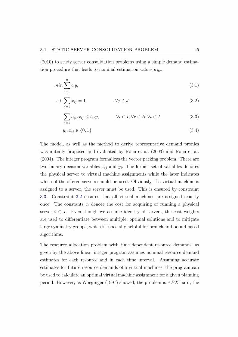
3.1. STATIC SERVER CONSOLIDATION PROBLEM 45
(2010) to study server consolidation problems using a simple demand estima-
tion procedure that leads to nominal estimation values ajtr.
min
n∑i=1
ciyi (3.1)
s.t.
m∑j=1
xij = 1 ,∀j ∈ J (3.2)
m∑j=1
ajtrxij ≤ biryi ,∀i ∈ I,∀r ∈ R, ∀t ∈ T (3.3)
yi, xij ∈ {0, 1} (3.4)
The model, as well as the method to derive representative demand profiles
was initially proposed and evaluated by Rolia et al. (2003) and Rolia et al.
(2004). The integer program formalizes the vector packing problem. There are
two binary decision variables xij and yi. The former set of variables denotes
the physical server to virtual machine assignments while the later indicates
which of the offered servers should be used. Obviously, if a virtual machine is
assigned to a server, the server must be used. This is ensured by constraint
3.3. Constraint 3.2 ensures that all virtual machines are assigned exactly
once. The constants ci denote the cost for acquiring or running a physical
server i ∈ I. Even though we assume identity of servers, the cost weights
are used to differentiate between multiple, optimal solutions and to mitigate
large symmetry groups, which is especially helpful for branch and bound based
algorithms.
The resource allocation problem with time dependent resource demands, as
given by the above linear integer program assumes nominal resource demand
estimates for each resource and in each time interval. Assuming accurate
estimates for future resource demands of a virtual machines, the program can
be used to calculate an optimal virtual machine assignment for a given planning
period. However, as Woeginger (1997) showed, the problem is APX-hard, the
46 CHAPTER 3. PROBLEM AND MODEL DEFINITIONS
1-dimensional bin packing problem is already NP -hard. Hence, we may not
expect the existence of computationally efficient, exact methods that scale
for large problem instances consisting of several hundreds of virtual machines
and require the use of relatively low capacitated physical servers that may host
only a small number of virtual machines - the problem becomes computational
harder with increasing |I|.
However, commercial as well as open-source solver packages can be used to
compute exact solutions for small scale problem instances. Even though
Speitkamp and Bichler (2010) solved moderate problem instances with up to
250 virtual machines using up to 288 time intervals within reasonable time
bounds, the physical servers sizes where chosen rather large: on average a
physical server was able to host more than 25 virtual machines. Despite the
computational complexity, we will use the basic model and some extensions
in this work to calculate consolidation plans and expectation baselines for dy-
namic workload management.
3.2 Consolidation Overheads Extension
One of the assumptions of the SSAPv model is the additivity of resource
demands when hosting virtual machines on shared hardware. While this as-
sumption may hold true for special hardware partitioning methods and for
some types of resources, it is not valid on commodity hardware for CPU de-
mands as shown by Iyer et al. (2009), Jerger et al. (2007), Govindan et al.
(2011), Nathuji et al. (2010) and Blagodurov et al. (2010). These works show
that application performance is severely affected by cache contention effects
that increase the amount of computing cycles required for the execution of an
instruction, which leads to increased CPU demands. Govindan et al. (2011)
proposes a measurement based approach to deal with application performance
degradation in server consolidation problems.
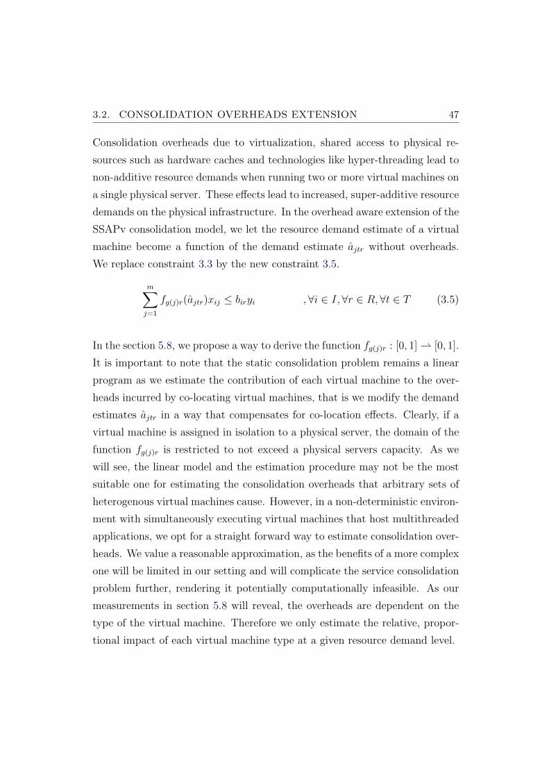
3.2. CONSOLIDATION OVERHEADS EXTENSION 47
Consolidation overheads due to virtualization, shared access to physical re-
sources such as hardware caches and technologies like hyper-threading lead to
non-additive resource demands when running two or more virtual machines on
a single physical server. These effects lead to increased, super-additive resource
demands on the physical infrastructure. In the overhead aware extension of the
SSAPv consolidation model, we let the resource demand estimate of a virtual
machine become a function of the demand estimate ajtr without overheads.
We replace constraint 3.3 by the new constraint 3.5.
m∑j=1
fg(j)r(ajtr)xij ≤ biryi ,∀i ∈ I,∀r ∈ R, ∀t ∈ T (3.5)
In the section 5.8, we propose a way to derive the function fg(j)r : [0, 1] ⇀ [0, 1].
It is important to note that the static consolidation problem remains a linear
program as we estimate the contribution of each virtual machine to the over-
heads incurred by co-locating virtual machines, that is we modify the demand
estimates ajtr in a way that compensates for co-location effects. Clearly, if a
virtual machine is assigned in isolation to a physical server, the domain of the
function fg(j)r is restricted to not exceed a physical servers capacity. As we
will see, the linear model and the estimation procedure may not be the most
suitable one for estimating the consolidation overheads that arbitrary sets of
heterogenous virtual machines cause. However, in a non-deterministic environ-
ment with simultaneously executing virtual machines that host multithreaded
applications, we opt for a straight forward way to estimate consolidation over-
heads. We value a reasonable approximation, as the benefits of a more complex
one will be limited in our setting and will complicate the service consolidation
problem further, rendering it potentially computationally infeasible. As our
measurements in section 5.8 will reveal, the overheads are dependent on the
type of the virtual machine. Therefore we only estimate the relative, propor-
tional impact of each virtual machine type at a given resource demand level.
48 CHAPTER 3. PROBLEM AND MODEL DEFINITIONS
3.3 Assignment Transition Problem with
Overheads
The SSAPv consolidation model, if applied to a single time interval t of a
multi-interval planning problem, say, the multi-interval problem has |T | = 24
time interval, gives a virtual machine to physical server assignment xtij that is
optimal for the single interval t. By solving the problem for each time interval
t ∈ T , we get the estimated amount of physical server required in each time
interval. However, the assignments xtij may differ largely from each other, that
is the virtual machines may be shuffled around on the physical servers if two
sequential time intervals t and t+1 are compared, which would lead to unneces-
sary virtual machine migrations. Therefore we propose a planning model that
can be used to minimize the required migrations necessary to transfer a data
centre from one optimal assignment xtij to the next optimal assignment xt+1ij .
The model can be used to define expectation baselines for dynamic workload
management methods. Due to changing resource demands of virtual machines,
assignments valid for a given time interval t may become infeasible which re-
quires the transition from one optimal assignment to the next. If we assume
to have available the estimates ajtr for time interval t and if we can defer from
the resource demand estimate the overhead for migrating a virtual machine at
the transition to t we can solve the assignment problem. Let mj denote the
estimated costs for migrating virtual machine j within the current transition
phase. Let wij denote the current assignments, where wij = 1 if virtual ma-
chine j is currently running on server i. Then the optimization problem, that
minimizes the amount of required servers by taking into account the resource
demand estimates of the future time intervals (t + 1, t + 2, ...) ∈ Tl is given
by replacing the objective function of the SSAPv model by the new objective
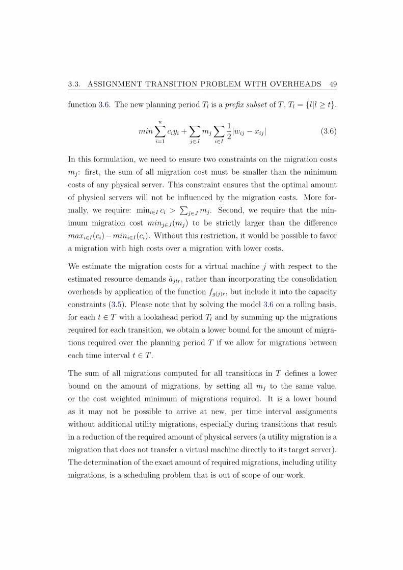
3.3. ASSIGNMENT TRANSITION PROBLEM WITH OVERHEADS 49
function 3.6. The new planning period Tl is a prefix subset of T , Tl = {l|l ≥ t}.
min
n∑i=1
ciyi +∑j∈J
mj
∑i∈I
1
2|wij − xij| (3.6)
In this formulation, we need to ensure two constraints on the migration costs
mj: first, the sum of all migration cost must be smaller than the minimum
costs of any physical server. This constraint ensures that the optimal amount
of physical servers will not be influenced by the migration costs. More for-
mally, we require: mini∈I ci >∑
j∈J mj. Second, we require that the min-
imum migration cost minj∈J(mj) to be strictly larger than the difference
maxi∈I(ci)−mini∈I(ci). Without this restriction, it would be possible to favor
a migration with high costs over a migration with lower costs.
We estimate the migration costs for a virtual machine j with respect to the
estimated resource demands ajtr, rather than incorporating the consolidation
overheads by application of the function fg(j)r, but include it into the capacity
constraints (3.5). Please note that by solving the model 3.6 on a rolling basis,
for each t ∈ T with a lookahead period Tl and by summing up the migrations
required for each transition, we obtain a lower bound for the amount of migra-
tions required over the planning period T if we allow for migrations between
each time interval t ∈ T .
The sum of all migrations computed for all transitions in T defines a lower
bound on the amount of migrations, by setting all mj to the same value,
or the cost weighted minimum of migrations required. It is a lower bound
as it may not be possible to arrive at new, per time interval assignments
without additional utility migrations, especially during transitions that result
in a reduction of the required amount of physical servers (a utility migration is a
migration that does not transfer a virtual machine directly to its target server).
The determination of the exact amount of required migrations, including utility
migrations, is a scheduling problem that is out of scope of our work.
Chapter 4
Data Set Description
As the United States Congress confronts budgeting challenges,
whether federal funding of scientific research is perceived as an
investment or a discretionary expense will have long-term conse-
quences.
”Budgeting for the long run”, Nature Materials Volume 10, Is-
sue 407, 2011
Our study relies on two distinct, real world data sets that we inspect to defer
typical data centre workload scenarios and to reason about resource alloca-
tion methods. Additionally, we use the first data set to gain insights into the
performance of short term demand prediction models. The second data set
serves us as a basis for deriving workload scenarios for a data centre bench-
mark. We will refer to the two data sets as resource demand traces and service
demand traces. As the data sets are fundamental to our work, we provide a
detailed analysis. The analysis will reveal the difficulties involved in forecast-
ing resource demands and will support our rational to investigate on average
demand conditions in our data centre benchmark which sets us apart from pre-
vious studies (Kumar et al. (2010), Chase et al. (2001), Gmach et al. (2009)
50
51
or Kusic and Kandasamy (2007)). The analysis of the first data set will be
important to understand why our benchmark scenarios contain demand level
dependent noise.
The resource demand traces are obtained from 259 standard SAP application
stacks. The traces contain data of about three months for CPU and main mem-
ory demands. Each trace is recorded at a frequency of five minutes, each entry
representing an average value over a five minute period. The set stems from a
diverse set of customers domiciled in different branches of industry. The second
set contains service demands for 50 core business processes that are executed
on distributed transaction processing systems of a large telecom provider. The
traces are recorded at a frequency of an hour, each record represents the aver-
age number of service requests for one of the business processes for an one hour
time interval. The traces also contain more than three months of data. The
telecom provider conducts business with private as well as business customers,
offering mobile telecom products as well as mobile data services. On weekdays,
the service demand is mainly issued by shop employees, customers, call center
agents and external sales partners using web-based application services. The
processes, triggered by a request for service, are related to the management
of retail customers including billing, customer data acquisition, phone number
management, tariff management, customer subscription and deactivation and
network provisioning. During night times, internal billing and customer rela-
tionship management systems operate in batch mode executing analytical jobs
that are also triggered by service requests. We consider the service demand
data set as representative for medium and large enterprises and base our data
centre benchmark on this set.
52 CHAPTER 4. DATA SET DESCRIPTION
4.1 Seasonal Patterns and Self-Similarity
Both data sets are comprised of time series that exhibit two seasonal compo-
nents: patterns of change that repeat themselves on a daily and weekly basis.
While the daily pattern correspond to business working days and hours, the
weekly pattern evolves from non-working hours during weekends.
To analyze seasonal patterns, auto-correlation functions are useful to deter-
mine the correlation for all pairs of observations which are separated by the
same lag. By means of the autocorrelation function, the degree of a linear
relationship between observations with the same time distance is measured
using the Pearson correlation coefficient. For instance, for time series contain-
ing observations of five-minute intervals, a lag of twelve measures the linear
relationship between the observations relative to the mean of the overall time
series between all pairs of observations which are one hour apart. For the
service demand data, a lag of twelve means measuring the correlation between
all pairs of observations which are twelve hours apart.
4.1.1 Resource Demand Traces
Figure 4.1 shows an example of a CPU demand trace over a single, extracted
week of the resource demand data set. Phases of high demands repeat on
a daily basis on the working days while the weekends are characterized by
constantly low demands. We also observe differences between the different
working days, e.g. demand peaks on Wednesday are much higher than those
on the following and preceding days. Peaks are rather sharp and occur seldom.
The example shows that although we may observe repeating patterns (the red
line is a smoothed version of the series, better showing the daily seasonalities),
the patterns are, to a certain extend, blurred by noise and large fluctuations
on short time scales. The different demand levels on neighboring days in
combination with sharp, sporadic demand spikes and the amount of noise may
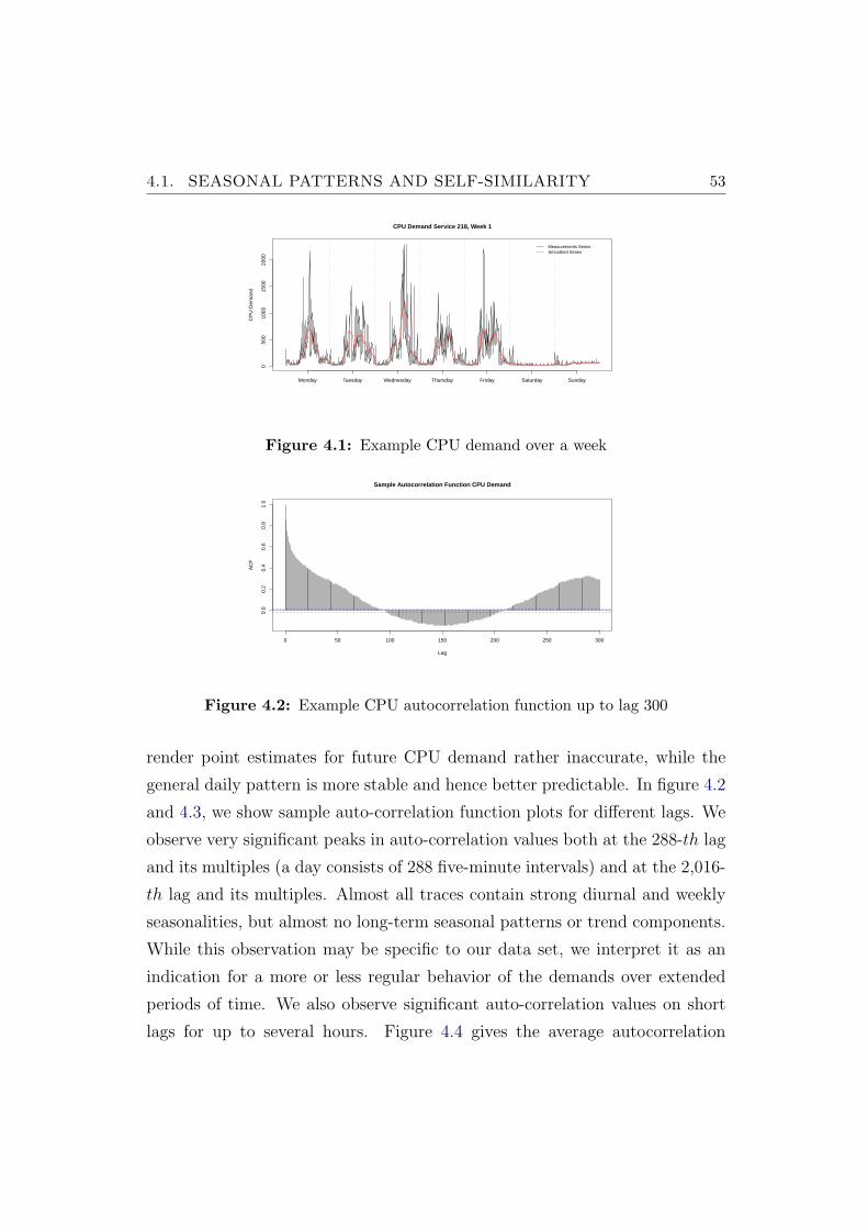
4.1. SEASONAL PATTERNS AND SELF-SIMILARITY 53
CPU Demand Service 218, Week 1
CP
U D
eman
d
050
010
0015
0020
00
Measurements SeriesSmoothed Series
Monday Tuesday Wednesday Thursday Friday Saturday Sunday
Figure 4.1: Example CPU demand over a week
0 50 100 150 200 250 300
0.0
0.2
0.4
0.6
0.8
1.0
Lag
AC
F
Sample Autocorrelation Function CPU Demand
Figure 4.2: Example CPU autocorrelation function up to lag 300
render point estimates for future CPU demand rather inaccurate, while the
general daily pattern is more stable and hence better predictable. In figure 4.2
and 4.3, we show sample auto-correlation function plots for different lags. We
observe very significant peaks in auto-correlation values both at the 288-th lag
and its multiples (a day consists of 288 five-minute intervals) and at the 2,016-
th lag and its multiples. Almost all traces contain strong diurnal and weekly
seasonalities, but almost no long-term seasonal patterns or trend components.
While this observation may be specific to our data set, we interpret it as an
indication for a more or less regular behavior of the demands over extended
periods of time. We also observe significant auto-correlation values on short
lags for up to several hours. Figure 4.4 gives the average autocorrelation
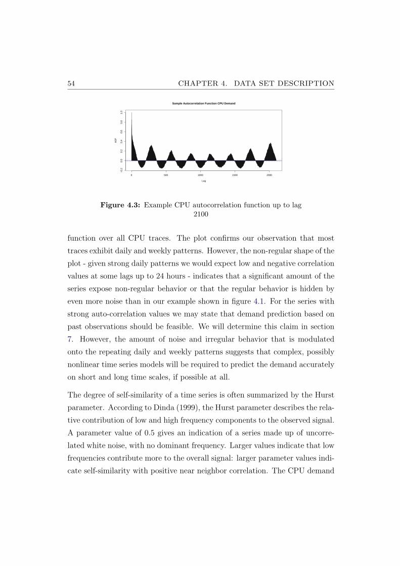
54 CHAPTER 4. DATA SET DESCRIPTION
0 500 1000 1500 2000
−0.
20.
00.
20.
40.
60.
81.
0
Lag
AC
F
Sample Autocorrelation Function CPU Demand
Figure 4.3: Example CPU autocorrelation function up to lag2100
function over all CPU traces. The plot confirms our observation that most
traces exhibit daily and weekly patterns. However, the non-regular shape of the
plot - given strong daily patterns we would expect low and negative correlation
values at some lags up to 24 hours - indicates that a significant amount of the
series expose non-regular behavior or that the regular behavior is hidden by
even more noise than in our example shown in figure 4.1. For the series with
strong auto-correlation values we may state that demand prediction based on
past observations should be feasible. We will determine this claim in section
7. However, the amount of noise and irregular behavior that is modulated
onto the repeating daily and weekly patterns suggests that complex, possibly
nonlinear time series models will be required to predict the demand accurately
on short and long time scales, if possible at all.
The degree of self-similarity of a time series is often summarized by the Hurst
parameter. According to Dinda (1999), the Hurst parameter describes the rela-
tive contribution of low and high frequency components to the observed signal.
A parameter value of 0.5 gives an indication of a series made up of uncorre-
lated white noise, with no dominant frequency. Larger values indicate that low
frequencies contribute more to the overall signal: larger parameter values indi-
cate self-similarity with positive near neighbor correlation. The CPU demand
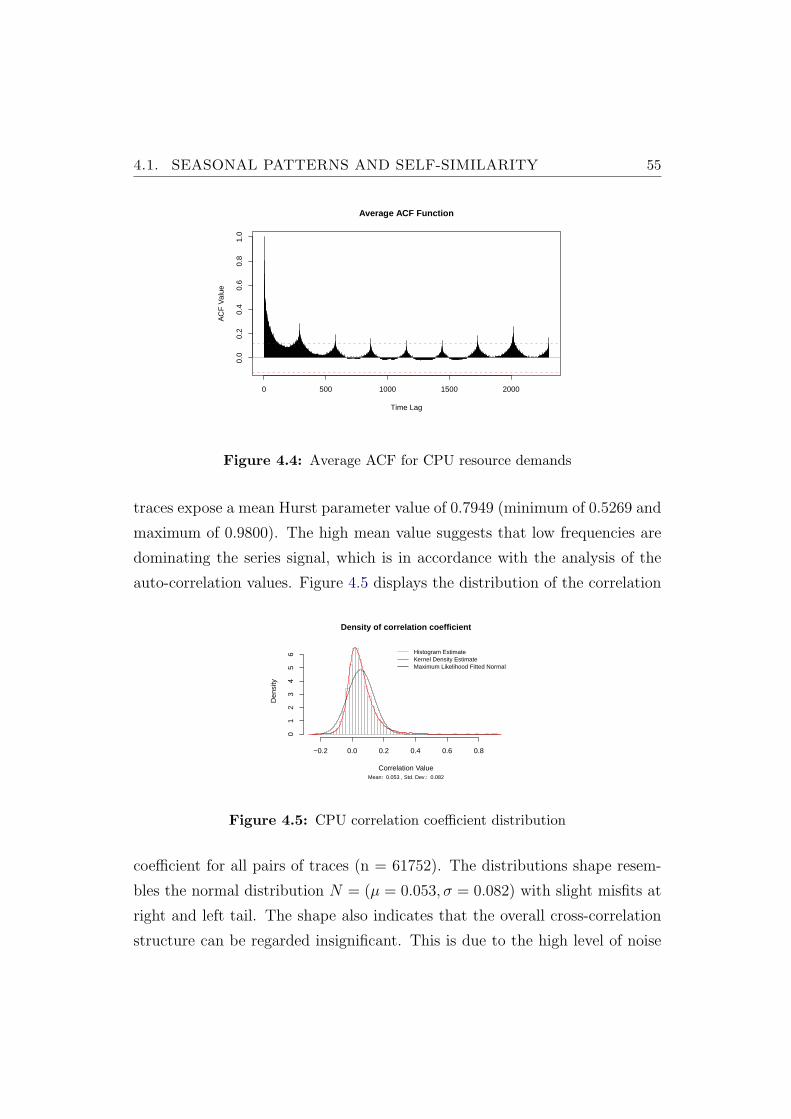
4.1. SEASONAL PATTERNS AND SELF-SIMILARITY 55
0 500 1000 1500 2000
0.0
0.2
0.4
0.6
0.8
1.0
Average ACF Function
Time Lag
AC
F V
alue
Figure 4.4: Average ACF for CPU resource demands
traces expose a mean Hurst parameter value of 0.7949 (minimum of 0.5269 and
maximum of 0.9800). The high mean value suggests that low frequencies are
dominating the series signal, which is in accordance with the analysis of the
auto-correlation values. Figure 4.5 displays the distribution of the correlation
Density of correlation coefficient
Mean: 0.053 , Std. Dev.: 0.082
Correlation Value
Den
sity
−0.2 0.0 0.2 0.4 0.6 0.8
01
23
45
6 Histogram EstimateKernel Density EstimateMaximum Likelihood Fitted Normal
Figure 4.5: CPU correlation coefficient distribution
coefficient for all pairs of traces (n = 61752). The distributions shape resem-
bles the normal distribution N = (µ = 0.053, σ = 0.082) with slight misfits at
right and left tail. The shape also indicates that the overall cross-correlation
structure can be regarded insignificant. This is due to the high level of noise
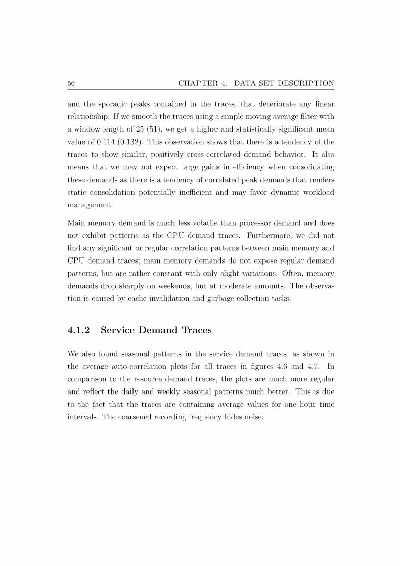
56 CHAPTER 4. DATA SET DESCRIPTION
and the sporadic peaks contained in the traces, that deteriorate any linear
relationship. If we smooth the traces using a simple moving average filter with
a window length of 25 (51), we get a higher and statistically significant mean
value of 0.114 (0.132). This observation shows that there is a tendency of the
traces to show similar, positively cross-correlated demand behavior. It also
means that we may not expect large gains in efficiency when consolidating
these demands as there is a tendency of correlated peak demands that renders
static consolidation potentially inefficient and may favor dynamic workload
management.
Main memory demand is much less volatile than processor demand and does
not exhibit patterns as the CPU demand traces. Furthermore, we did not
find any significant or regular correlation patterns between main memory and
CPU demand traces; main memory demands do not expose regular demand
patterns, but are rather constant with only slight variations. Often, memory
demands drop sharply on weekends, but at moderate amounts. The observa-
tion is caused by cache invalidation and garbage collection tasks.
4.1.2 Service Demand Traces
We also found seasonal patterns in the service demand traces, as shown in
the average auto-correlation plots for all traces in figures 4.6 and 4.7. In
comparison to the resource demand traces, the plots are much more regular
and reflect the daily and weekly seasonal patterns much better. This is due
to the fact that the traces are containing average values for one hour time
intervals. The coarsened recording frequency hides noise.
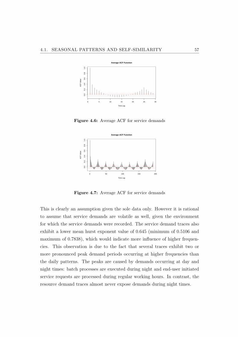
4.1. SEASONAL PATTERNS AND SELF-SIMILARITY 57
0 5 10 15 20 25 30
0.0
0.2
0.4
0.6
0.8
1.0
Average ACF Function
Time Lag
AC
F V
alue
Figure 4.6: Average ACF for service demands
0 50 100 150 200
0.0
0.2
0.4
0.6
0.8
1.0
Average ACF Function
Time Lag
AC
F V
alue
Figure 4.7: Average ACF for service demands
This is clearly an assumption given the sole data only. However it is rational
to assume that service demands are volatile as well, given the environment
for which the service demands were recorded. The service demand traces also
exhibit a lower mean hurst exponent value of 0.645 (minimum of 0.5106 and
maximum of 0.7838), which would indicate more influence of higher frequen-
cies. This observation is due to the fact that several traces exhibit two or
more pronounced peak demand periods occurring at higher frequencies than
the daily patterns. The peaks are caused by demands occurring at day and
night times: batch processes are executed during night and end-user initiated
service requests are processed during regular working hours. In contrast, the
resource demand traces almost never expose demands during night times.
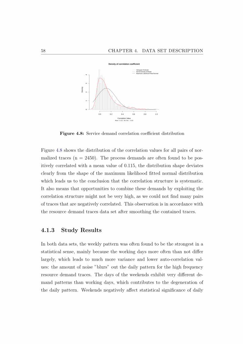
58 CHAPTER 4. DATA SET DESCRIPTION
Density of correlation coefficient
Mean: 0.115 , Std. Dev.: 0.163
Correlation Value
Den
sity
0.0 0.2 0.4 0.6 0.8 1.0
01
23
4
Histogram EstimateKernel Density EstimateMaximum Likelihood Fitted Normal
Figure 4.8: Service demand correlation coefficient distribution
Figure 4.8 shows the distribution of the correlation values for all pairs of nor-
malized traces (n = 2450). The process demands are often found to be pos-
itively correlated with a mean value of 0.115, the distribution shape deviates
clearly from the shape of the maximum likelihood fitted normal distribution
which leads us to the conclusion that the correlation structure is systematic.
It also means that opportunities to combine these demands by exploiting the
correlation structure might not be very high, as we could not find many pairs
of traces that are negatively correlated. This observation is in accordance with
the resource demand traces data set after smoothing the contained traces.
4.1.3 Study Results
In both data sets, the weekly pattern was often found to be the strongest in a
statistical sense, mainly because the working days more often than not differ
largely, which leads to much more variance and lower auto-correlation val-
ues: the amount of noise ”blurs” out the daily pattern for the high frequency
resource demand traces. The days of the weekends exhibit very different de-
mand patterns than working days, which contributes to the degeneration of
the daily pattern. Weekends negatively affect statistical significance of daily
4.2. STATISTICAL ANALYSIS 59
patterns which becomes evident when excluding them from the traces. There-
fore the daily pattern was also significant and is of more interest to us than
the low demand phases during the weekends. The low demand phases during
the weekends lead to statistically stronger weekly patterns as can be deferred
from power spectral density periodogram plots not shown here. As it is evident
that the periods of low demand on weekends do not contribute to our research
goals, we focus on working days and exclude weekends from our data sets in
the following sections and chapters.
4.2 Statistical Analysis
We have seen that there exist seasonal demand patterns in the two data sets.
In the following subsections, we will give descriptive statistics on the filtered
traces: we exclude weekends from the two sets.
4.2.1 Resource Demand Traces
The resource demand traces expose complex behavior over a wide range of
time scales: repeating patterns on longer time scales as induced by positive
auto-correlation values on long lags and heavily noised behavior on short time
scales. In summary, we observe self-similarity which induces variation across
long and short time scales and also induces that even high level of smoothing
does not decrease the observed variance as we still find high variance due to
long term, seasonal behavior. This observation may lead to the assumption
that non-stationary stochastic processes with long memory behavior may de-
scribe the series well as suggested by Dinda (1999). However, the demand
distributions show complex, long tailed behavior that renders the precondition
for linear time series models problematic, that the error terms are independent
identically-distributed random variables, sampled from a normal distribution.
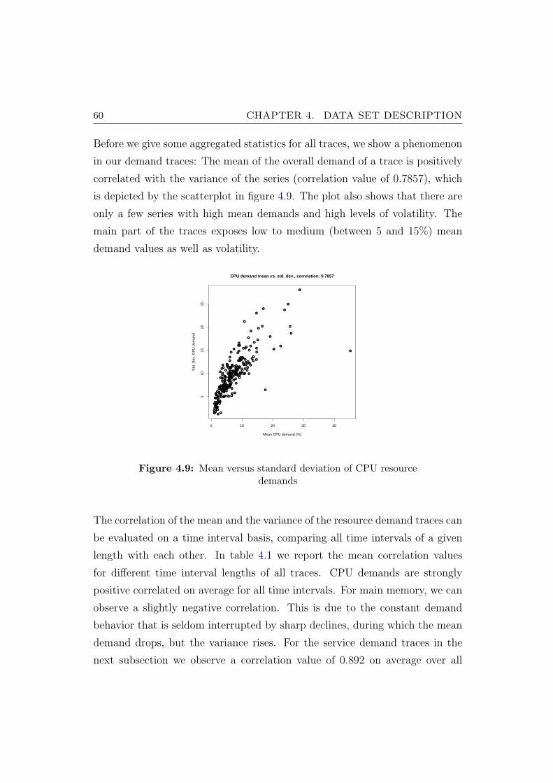
60 CHAPTER 4. DATA SET DESCRIPTION
Before we give some aggregated statistics for all traces, we show a phenomenon
in our demand traces: The mean of the overall demand of a trace is positively
correlated with the variance of the series (correlation value of 0.7857), which
is depicted by the scatterplot in figure 4.9. The plot also shows that there are
only a few series with high mean demands and high levels of volatility. The
main part of the traces exposes low to medium (between 5 and 15%) mean
demand values as well as volatility.
●
●
●
●
●
●
●
●
●
●
●●
●
●
●●
●
●
●
●
●
●
●
● ●●
●
●
●
●
●
●●
●
●
●
●
●
●
●
●
●
●
●
●
●
●
●
●●
●
●
●
●
●
●
●
●●
●
●
●
●
●
●
●
●
●
●
●
●
●
●
●●
●
● ●
●
●
●
●
●
●●
●
●
● ●
●
●
●
●
●
●●
●
●
●
●
●
●
●
●
●
●
●
●
●
●
●
●
●
●
●
●
●
●
●●
●
●
●
●
●
●
●
●●
●
●
●
●
●
●
●
●
●
●
●
●
●
●
●●
●
●
●
●●
●
●
●
●
●
●
●
●
●
●
●●●
●
●
●●
●
●
●
●
●
●
●
●
●
●
●
●
●
●●
●
●
●
●
●
●
●
●
●●
●
●
●
●●
●
●
●
●
●
●
●
●
●
●
●
●●
●●
●
●
●●
●
●
●●
●
●
●●
●●
●●
●
●
●
●
●
●
●
●
●
●●
●
●
●
●
●
●
●
●
●
●
●
●
●●
●
●
●
●
0 10 20 30 40
510
1520
25
CPU demand mean vs. std. dev., correlation: 0.7857
Mean CPU demand (%)
Std
. Dev
. CP
U d
eman
d
Figure 4.9: Mean versus standard deviation of CPU resourcedemands
The correlation of the mean and the variance of the resource demand traces can
be evaluated on a time interval basis, comparing all time intervals of a given
length with each other. In table 4.1 we report the mean correlation values
for different time interval lengths of all traces. CPU demands are strongly
positive correlated on average for all time intervals. For main memory, we can
observe a slightly negative correlation. This is due to the constant demand
behavior that is seldom interrupted by sharp declines, during which the mean
demand drops, but the variance rises. For the service demand traces in the
next subsection we observe a correlation value of 0.892 on average over all
4.2. STATISTICAL ANALYSIS 61
traces for one hour time intervals.
Type Resource Mean
5 Minute Interval CPU 0.799
5 Minute Interval RAM -0.38
1 Hour Interval CPU 0.817
1 Hour Interval RAM -0.016
3 Hours Interval CPU 0.809
3 Hours Periods RAM -0.074
Table 4.1: Resource demand correlation for time intervals
These correlation findings are in accordance with the observation presented in
Burgess et al. (2002). Figure 4.1 shows the time dependent volatility of the
CPU resource demand distribution for an example trace. We can easily see
from the chart that periods of high demand intensity are governed by larger
deviations. While our observations apply to a macroscopic view, Andreolini
et al. (2008) also found this behavior for various, heterogenous service demand
scenarios and changing service demand mixes at the microscopic level for a
monitoring frequency of seconds. We can also observe a phenomenon which
is referred to as volatility clustering in the field of econometrics. Volatility
clustering refers to the observation, that large variation in time series tend to be
followed by large variations, either positive or negative changes, and periods of
low volatility tend to be followed by low volatility. We may consequently expect
forecasts to be accurate during periods of low demand and rather inaccurate for
periods of high demands. We also find that demand peaks vary significantly in
aspects such as steepness, magnitude or level, duration, and temporal locality.
Table 4.2 summarizes the normalized traces, each trace is normalized to its
maximum value and expressed in percent, by giving averages for each metric.
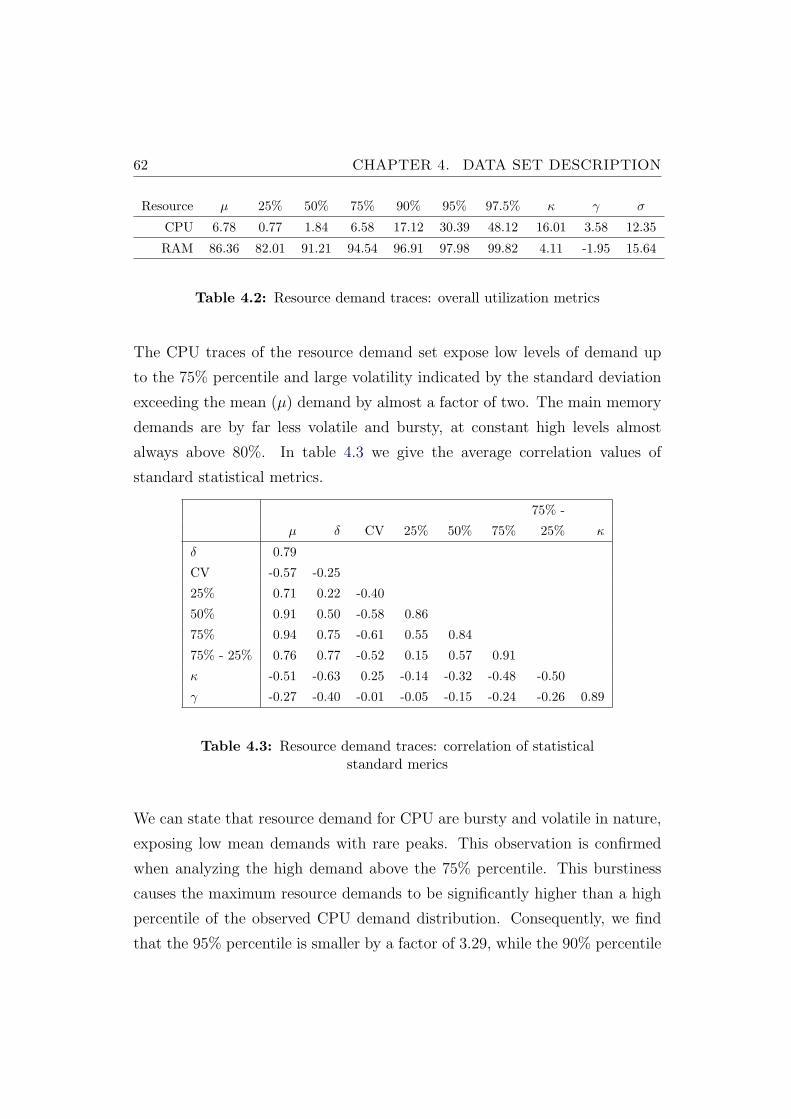
62 CHAPTER 4. DATA SET DESCRIPTION
Resource µ 25% 50% 75% 90% 95% 97.5% κ γ σ
CPU 6.78 0.77 1.84 6.58 17.12 30.39 48.12 16.01 3.58 12.35
RAM 86.36 82.01 91.21 94.54 96.91 97.98 99.82 4.11 -1.95 15.64
Table 4.2: Resource demand traces: overall utilization metrics
The CPU traces of the resource demand set expose low levels of demand up
to the 75% percentile and large volatility indicated by the standard deviation
exceeding the mean (µ) demand by almost a factor of two. The main memory
demands are by far less volatile and bursty, at constant high levels almost
always above 80%. In table 4.3 we give the average correlation values of
standard statistical metrics.
75% -
µ δ CV 25% 50% 75% 25% κ
δ 0.79
CV -0.57 -0.25
25% 0.71 0.22 -0.40
50% 0.91 0.50 -0.58 0.86
75% 0.94 0.75 -0.61 0.55 0.84
75% - 25% 0.76 0.77 -0.52 0.15 0.57 0.91
κ -0.51 -0.63 0.25 -0.14 -0.32 -0.48 -0.50
γ -0.27 -0.40 -0.01 -0.05 -0.15 -0.24 -0.26 0.89
Table 4.3: Resource demand traces: correlation of statisticalstandard merics
We can state that resource demand for CPU are bursty and volatile in nature,
exposing low mean demands with rare peaks. This observation is confirmed
when analyzing the high demand above the 75% percentile. This burstiness
causes the maximum resource demands to be significantly higher than a high
percentile of the observed CPU demand distribution. Consequently, we find
that the 95% percentile is smaller by a factor of 3.29, while the 90% percentile
4.2. STATISTICAL ANALYSIS 63
yields a reduction of a factor up to 5.84, the median even a factor of over 50.
An intuitive interpretation for a data centre operator is as follows: if CPU is
allocated according to the average 90% demand percentile, it would be pos-
sible to support almost six times more virtual machines on a single physical
server (assuming equal demand levels for all virtual machines) compared to a
resource allocation scheme that follows the maximum CPU demands. How-
ever, resource provisioning according to lower percentiles comes at the price
of possible overloads. These impressive overbooking ratios may not be realiz-
able but indicate a large potential for costs reductions, if resource shortages
are acceptable. The same motivation for resource overbooking is given by Ur-
gaonkar et al. (2009), who analyze steady-state CPU demands of several types
of applications. However, their analyses is only valid for very lightly utilized
applications as the following experiment we conducted demonstrates.
In figure 4.10 we depict the CPU demands of a monolithic application con-
figuration (please refer to subsection 5.3 for more details) of the SpecjEnter-
prise2010 benchmark system we use in our work. We exercised the application
with three different amounts of constant service demand. As we can see, the
long tails of the demand distribution diminish with increasing service demand
and CPU demands for constant service demand. Low service demand levels
expose more outlying and exceptional demand values. As depicted on the right
hand side of figure 4.10 also document the correlation of mean demands and
their variance.
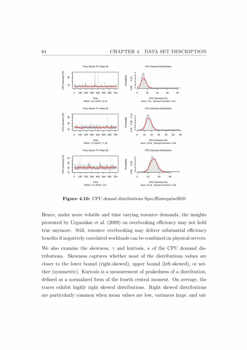
64 CHAPTER 4. DATA SET DESCRIPTION
Time
0 100 200 300 400 500 600 700
1030
Time Series TX−Rate 30
RMSE: 2.51 MAPE: 24.25
CP
U D
eman
d (%
)
Time
0 100 200 300 400 500 600 700
1030
50
Time Series TX−Rate 60
RMSE: 3.79 MAPE: 17.48
CP
U D
eman
d (%
)
Time
0 100 200 300 400 500 600 700
1030
5070
Time Series TX−Rate 90
RMSE: 6.41 MAPE: 16.2
CP
U D
eman
d (%
)
0 10 20 30 40
0.00
0.15
CPU Demand Distribution
Mean: 6.54 , Standard Deviation: 2.59CPU Demand (%)
Pro
babi
lity
0 10 20 30 40 50 60
0.00
0.06
0.12
CPU Demand Distribution
Mean: 16.06 , Standard Deviation: 3.86CPU Demand (%)
Pro
babi
lity
0 20 40 60
0.00
0.04
CPU Demand Distribution
Mean: 30.18 , Standard Deviation: 6.58CPU Demand (%)
Pro
babi
lity
Figure 4.10: CPU demad distributions SpecJEnterprise2010
Hence, under more volatile and time varying resource demands, the insights
presented by Urgaonkar et al. (2009) on overbooking efficiency may not hold
true anymore. Still, resource overbooking may deliver substantial efficiency
benefits if negatively correlated workloads can be combined on physical servers.
We also examine the skewness, γ and kurtosis, κ of the CPU demand dis-
tributions. Skewness captures whether most of the distributions values are
closer to the lower bound (right-skewed), upper bound (left-skewed), or nei-
ther (symmetric). Kurtosis is a measurement of peakedness of a distribution,
defined as a normalized form of the fourth central moment. On average, the
traces exhibit highly right skewed distributions. Right skewed distributions
are particularly common when mean values are low, variances large, and val-
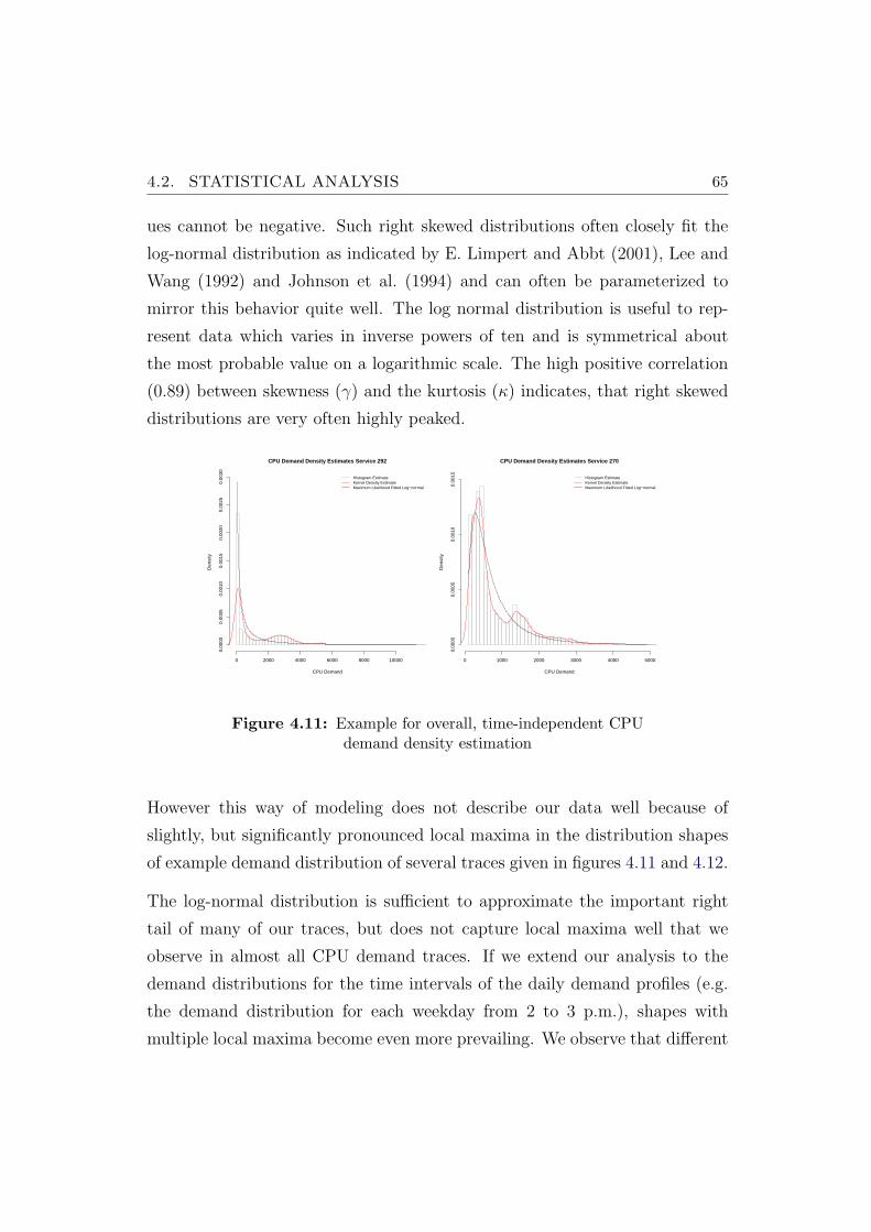
4.2. STATISTICAL ANALYSIS 65
ues cannot be negative. Such right skewed distributions often closely fit the
log-normal distribution as indicated by E. Limpert and Abbt (2001), Lee and
Wang (1992) and Johnson et al. (1994) and can often be parameterized to
mirror this behavior quite well. The log normal distribution is useful to rep-
resent data which varies in inverse powers of ten and is symmetrical about
the most probable value on a logarithmic scale. The high positive correlation
(0.89) between skewness (γ) and the kurtosis (κ) indicates, that right skewed
distributions are very often highly peaked.
CPU Demand Density Estimates Service 292
CPU Demand
Den
sity
0 2000 4000 6000 8000 10000
0.00
000.
0005
0.00
100.
0015
0.00
200.
0025
0.00
30
Histogram EstimateKernel Density EstimateMaximum Likelihood Fitted Log−normal
CPU Demand Density Estimates Service 270
CPU Demand
Den
sity
0 1000 2000 3000 4000 5000
0.00
000.
0005
0.00
100.
0015 Histogram Estimate
Kernel Density EstimateMaximum Likelihood Fitted Log−normal
Figure 4.11: Example for overall, time-independent CPUdemand density estimation
However this way of modeling does not describe our data well because of
slightly, but significantly pronounced local maxima in the distribution shapes
of example demand distribution of several traces given in figures 4.11 and 4.12.
The log-normal distribution is sufficient to approximate the important right
tail of many of our traces, but does not capture local maxima well that we
observe in almost all CPU demand traces. If we extend our analysis to the
demand distributions for the time intervals of the daily demand profiles (e.g.
the demand distribution for each weekday from 2 to 3 p.m.), shapes with
multiple local maxima become even more prevailing. We observe that different
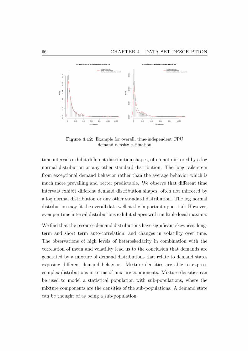
66 CHAPTER 4. DATA SET DESCRIPTION
CPU Demand Density Estimates Service 312
CPU Demand
Den
sity
0 2000 4000 6000 8000 10000 12000
0e+
002e
−04
4e−
046e
−04
8e−
041e
−03
Histogram EstimateKernel Density EstimateMaximum Likelihood Fitted Log−normal
CPU Demand Density Estimates Service 300
CPU DemandD
ensi
ty
0 2000 4000 6000 8000 10000
0.00
000.
0005
0.00
100.
0015
Histogram EstimateKernel Density EstimateMaximum Likelihood Fitted Log−normal
Figure 4.12: Example for overall, time-independent CPUdemand density estimation
time intervals exhibit different distribution shapes, often not mirrored by a log
normal distribution or any other standard distribution. The long tails stem
from exceptional demand behavior rather than the average behavior which is
much more prevailing and better predictable. We observe that different time
intervals exhibit different demand distribution shapes, often not mirrored by
a log normal distribution or any other standard distribution. The log normal
distribution may fit the overall data well at the important upper tail. However,
even per time interval distributions exhibit shapes with multiple local maxima.
We find that the resource demand distributions have significant skewness, long-
term and short term auto-correlation, and changes in volatility over time.
The observations of high levels of heteroskedacity in combination with the
correlation of mean and volatility lead us to the conclusion that demands are
generated by a mixture of demand distributions that relate to demand states
exposing different demand behavior. Mixture densities are able to express
complex distributions in terms of mixture components. Mixture densities can
be used to model a statistical population with sub-populations, where the
mixture components are the densities of the sub-populations. A demand state
can be thought of as being a sub-population.
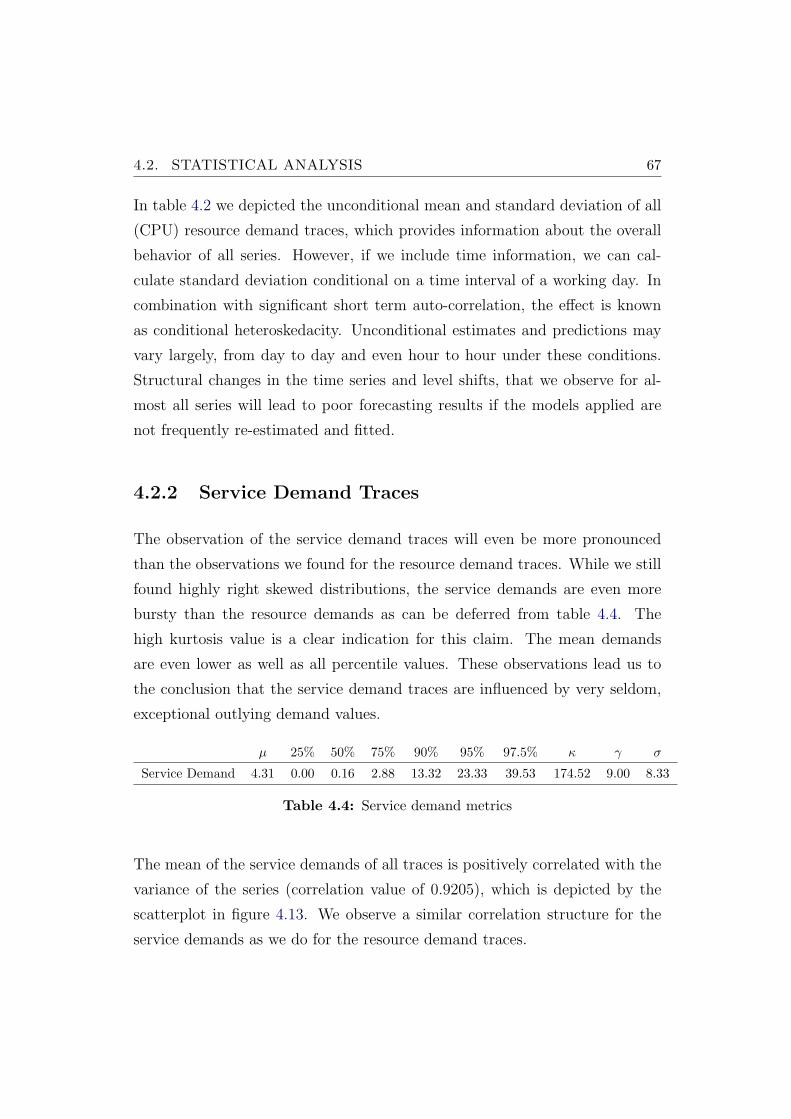
4.2. STATISTICAL ANALYSIS 67
In table 4.2 we depicted the unconditional mean and standard deviation of all
(CPU) resource demand traces, which provides information about the overall
behavior of all series. However, if we include time information, we can cal-
culate standard deviation conditional on a time interval of a working day. In
combination with significant short term auto-correlation, the effect is known
as conditional heteroskedacity. Unconditional estimates and predictions may
vary largely, from day to day and even hour to hour under these conditions.
Structural changes in the time series and level shifts, that we observe for al-
most all series will lead to poor forecasting results if the models applied are
not frequently re-estimated and fitted.
4.2.2 Service Demand Traces
The observation of the service demand traces will even be more pronounced
than the observations we found for the resource demand traces. While we still
found highly right skewed distributions, the service demands are even more
bursty than the resource demands as can be deferred from table 4.4. The
high kurtosis value is a clear indication for this claim. The mean demands
are even lower as well as all percentile values. These observations lead us to
the conclusion that the service demand traces are influenced by very seldom,
exceptional outlying demand values.
µ 25% 50% 75% 90% 95% 97.5% κ γ σ
Service Demand 4.31 0.00 0.16 2.88 13.32 23.33 39.53 174.52 9.00 8.33
Table 4.4: Service demand metrics
The mean of the service demands of all traces is positively correlated with the
variance of the series (correlation value of 0.9205), which is depicted by the
scatterplot in figure 4.13. We observe a similar correlation structure for the
service demands as we do for the resource demand traces.
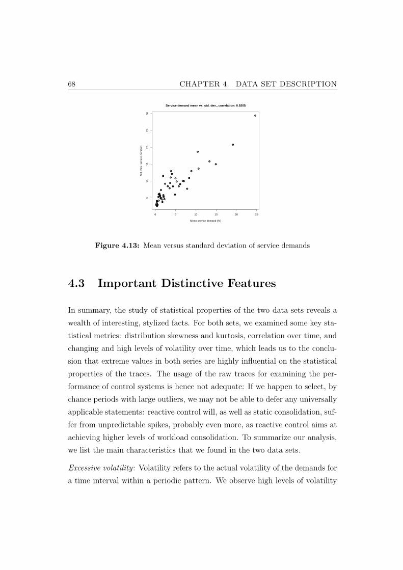
68 CHAPTER 4. DATA SET DESCRIPTION
●
●
●
●
●
●●
●
●
●
●
●
●
●
●
●
●
●
●
●
●
●
●
●
●●
●
●
●
●
●
●
●
●
●
●
●
●
●
●
●
●
●
●
●
●
●
●
●
●
0 5 10 15 20 25
510
1520
2530
Service demand mean vs. std. dev., correlation: 0.9205
Mean service demand (%)
Std
. Dev
. ser
vice
dem
and
Figure 4.13: Mean versus standard deviation of service demands
4.3 Important Distinctive Features
In summary, the study of statistical properties of the two data sets reveals a
wealth of interesting, stylized facts. For both sets, we examined some key sta-
tistical metrics: distribution skewness and kurtosis, correlation over time, and
changing and high levels of volatility over time, which leads us to the conclu-
sion that extreme values in both series are highly influential on the statistical
properties of the traces. The usage of the raw traces for examining the per-
formance of control systems is hence not adequate: If we happen to select, by
chance periods with large outliers, we may not be able to defer any universally
applicable statements: reactive control will, as well as static consolidation, suf-
fer from unpredictable spikes, probably even more, as reactive control aims at
achieving higher levels of workload consolidation. To summarize our analysis,
we list the main characteristics that we found in the two data sets.
Excessive volatility : Volatility refers to the actual volatility of the demands for
a time interval within a periodic pattern. We observe high levels of volatility
4.3. IMPORTANT DISTINCTIVE FEATURES 69
for one hour time intervals in both data sets: the mean is mostly much lower
than the standard deviation. The traces exhibit relatively low mean demand
but very high variability, measured by the standard deviation. The maximum
demands often exceed the mean demand by an order of magnitude and more,
depending on the time of the day and time of the week. The high volatility,
also observed by Dinda (1999) in a grid computing environment, indicates that
short term time series prediction algorithms may be used to predict workload
on short time scales. Long term forecasting models are very unlikely to predict
sporadic spikes and should not. Including outliers in the estimation procedure
will lead to biased predictions and overly pessimistic demand estimates.
Volatility and heteroskedacity : The demand level (mean demand in a time
interval) is strongly positively correlated with demand volatility. Moreover,
demand level and volatility show the same type of extended or long mem-
ory behavior. Measures of volatility, such as the standard deviation and the
inter quartile range, are strongly positive correlated with the mean demand
in time intervals. Consequently demands with a high mean will also tend to
have a large standard deviation and maximum. The correlation indicates het-
eroskedacity which defeats most classical time series models that are based
on regression techniques for parameter estimation. We may also state, that
up to a certain demand level, time series prediction methods may be more
efficient on traces with higher demand levels: the autocorrelation is more dis-
tinct, patterns are more explicit (the Hurst exponent and the mean demand
are positively correlated for the resource demand traces) than for traces with
low demand. Traces with very high demand levels lead expose rather extreme
volatility that will make short term forecasting methods unreliable.
Volatility clustering : as noted by Mandelbrot (1963), large changes tend to be
followed by large changes, of either sign, and small changes tend to be followed
by small changes.
Heavy tails : the unconditional distribution of resource demands displays a
70 CHAPTER 4. DATA SET DESCRIPTION
heavy tail with positive excess kurtosis. Excess kurtosis measures the fatness
of the tails of a distribution. Positive kurtosis is the degree of peakedness of
a distribution, defined as a normalized form of the fourth central moment.
Heavy tails induce that there is a higher than normal probability of large
demand values. That is, excess kurtosis indicates that the volatility of the
demands is itself highly volatile.
Long tails : very often, the probability of experiencing large demand levels
can not be described by heavy tailed distributions since there is often an ag-
glomeration of extremely large valued observations. Long tails are typically
found in exponential and Zipf-like type distributions as well as the log-normal
distribution. Exceptional demand values cause long tails.
Right-skewed distributions : Most of the distributions values are closer to the
lower bound, but exhibit complex distributions that are not well-fitted by
standard distributions. Under these conditions, the computation of confidence
intervals for demand levels may not be a reasonable operation.
Auto-correlation: Time series analysis of the traces shows that demands are
strongly autocorrelated over short and long time scales. The autocorrelation
function typically decays very slowly while the raw periodogram often shows
two dominating frequencies (weekly frequency is the strongest followed by a
daily frequency). However, the high auto-correlation values on short legs in-
duce complex frequency domain behavior that requires autoregressive predic-
tion models of high order.

Chapter 5
Experimental Data Centre
Testbed
”If today were the last day of my life, would I want to do what I
am about to do today ?” And whenever the answer has been ”No”
for too many days in a row, I know I need to change something.
by Steve Jobs, Address at Stanford University (2005)
In this chapter we describe the experimental testbed used to exercise a reactive
control system and static server consolidation under real world conditions. The
testbed consists of a method to generate data centre benchmark scenarios, a
virtualized infrastructure, a component that handles the execution life-cycle of
benchmark runs in a fully automated way based on a set of configuration files
and a control system in charge of taking virtual machine placement decisions
in real-time. Figure 5.1 depicts the testbed in a schematic way. We will give
more details on the testbed and its components in the following subsections.
71

72 CHAPTER 5. EXPERIMENTAL DATA CENTRE TESTBED
Storage
Server 2
Storage
Server 1
Control
Server 1
CONTROL
MASTER
BLASTER
SCENARIO
GENERATOR
!"#"$
%&'()*#(%+$
SUT
Server 1
SUT
SUT
SUT
Server 6
SUT
SUT
Load
Generator
Server 1
MASTER
DRIVER
Load
Generator
Server 4
MASTER
DRIVER
Layer 2 Switch
. . .
. . .
Figure 5.1: Testbed system overview
5.1 Testbed Workflow and Components
We describe the components of the testbed in a contextual way by depict-
ing the workflow used to execute experiment runs and measurements used in
this work. Figure 5.2 shows the workflow using an activity diagram. The
!""#$%&$'()*+,)$
-./0$!123,1$
4,),1/5,$
",132*,$!,6/)0$
7.88,*5$9:);6,$
"5/;<;*<$
9,*,23,$
7.)=>:1/;.)$
?28,<$",)0$9:);6,$
"5/;<;*<$"5.@$!,6/)0$
4,),1/;.)$
'/<5,1$A8/<5,1$
7.)51.8$"B<5,6$
-./0$'/<5,1$
CD$
!,@8.B$
7.)=>:1/;.)$
?28,<$
",5:@$
E)F1/G
<51:*5:1,$
"5/15$
A,)*+6/1H$
"*,)/12.$9:)$
"5/15$7.)51.8$
"B<5,6$
"5.@$7.)51.8$
"B<5,6$
7.88,*5$
'.)25.12)>$
!/5/$
IJ,*:5,$7.)51.8$
"51/5,>B$
A,)*+6/1H$"*,)/12.$4,),1/5.1$4,),1/5,$
A,)*+6/1H$
"*,)/12.$
K)/8B<,$
'.)25.12)>$!/5/$
'.)25.1$-./0$
4,),1/5.1<$
E)2;/82L,$
"*,)/12.$
9:)$
M/25$?.1$
"*,)/12.$
"5/15$
E)2;/5,$!,6/)0$
4,),1/;.)$
"5.@$
"*,)/12.$
9:)$
7.88,*5$
"*,)/12.$
"5/;<;*<$
9,*,23,$
7.)=>:1/;.)$
?28,<$
",)0$
'.)25.12)>$
!/5/$
",)0$
'.)25.12)>$
!/5/$
9,*,23,$
7.)=>:1/;.)$
?28,<$
Figure 5.2: Testbed workflow overview
benchmark scenario generator is a set of scripts that are used to define service
demand for each system under test (SUT). It can be parameterized to control
5.1. TESTBED WORKFLOW AND COMPONENTS 73
the amount of virtual machines in a scenario, their resource demands relative
to the capacities of a SUT physical server, the type of application configuration
of a single enterprise application (whether it will be deployed in a distributed
or monolithic way) and the volatility and shape of the service demands it will
serve. The generator prepares configuration files used by the Master Blaster
to control the execution of a benchmark run. The Master Blaster is a collec-
tion of Maven plugins that can be orchestrated for scenario run execution. A
benchmark run is the execution of a benchmark scenario with a specific set
of parameters for the control system. The execution workflow first checks the
scenario configuration for inconsistencies or errors as well as the availability
of all required virtual machines and physical servers. If the infrastructure is
found to be in conformance with the scenario configuration, all required vir-
tual machines on the SUT physical servers, as well as the virtual machines
required for service demand generation are assigned the configured resources
such as main memory, virtual CPU, CPU scheduler weights and caps as well
as network bandwidth allocation. According to the assignments computed
for the benchmark scenario, the virtual machines are started on the physical
servers. Once the setup process is complete for all virtual machines, the Master
Blaster distributes the required configuration files to the control system, the
load master, load drivers and the SUT applications, all running in dedicated
virtual machines. After the configuration files are distributed, the SUTs are
configured and populated with the required data to support a given amount of
virtual users. Application configuration information includes memory buffer
sizes, maximum allowed connections for the databases systems or minimum
and maximum heap space for the application servers, load drivers and load
masters. Each run is setup in this way, ensuring consistency across all runs
of a scenario. A run is started by activating all load masters according to a
predefined activation schedule which is necessary as a parallel warm up of all
SUTs would lead to severe overloads on the physical servers and a breakdown
of the storage servers. After the run initialization schedule is executed, the
74 CHAPTER 5. EXPERIMENTAL DATA CENTRE TESTBED
control system is started and the benchmark run starts. The control system
executes a configurable control strategy that is supplied with required con-
figuration parameters. During the run, the Master Blaster monitors all load
masters, checking the health of their execution status. A benchmark run is
aborted in case a load master reports misbehavior or can not be contacted
for a certain period of time. The same applies to the control system: if a
control action fails, or the control system is not able to monitor the physical
infrastructure anymore, the benchmark run is aborted.
Upon successful completion of a benchmark run, the Master Blaster shuts
down the control system and collects resource demand, virtual machine place-
ment, live migration log and response time monitoring traces from the control
system and the load masters for subsequent inspection.
5.2 Workload Generator Implementation
Most workload generators are not designed to support time varying workloads
or service request issued by virtual users. As an example, the well known tool
Httperf (Httperf, 2012) can be used to generate requests for web application
performance testing, but only at a fixed, constant rate. Therefore, we required
a flexible load testing framework that supports time varying amounts of virtual
users to emulate real world service demands. As the Faban framework (Faban,
2012) provides this capability and is already used to drive well accepted indus-
try benchmarks we decide to re-use the framework for our benchmark system.
Faban is a lightweight framework that is scalable across a large number of load
generation nodes and provides the required time synchronization between all
participating systems and automated application performance measurements
such as throughput and response times. All involved physical and virtual ma-
chines, their network addresses, access credentials, file and directory paths,
and application component settings are stored in the scenario configuration.
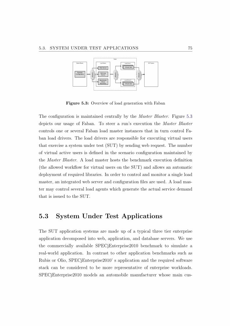
5.3. SYSTEM UNDER TEST APPLICATIONS 75
!""#$%&$'()*+,)$
Faban
-.$
Load Master
Web Server
SLA Log
Server
Benchmark
Driver
Repository
Load Driver !
Load Driver N
Virtual User Virtual User
Virtual User Virtual User
SUT System Master Blaster
Scenario
Configuration
/,01
234$
/,01
234$
/,01
234$
Figure 5.3: Overview of load generation with Faban
The configuration is maintained centrally by the Master Blaster. Figure 5.3
depicts our usage of Faban. To steer a run’s execution the Master Blaster
controls one or several Faban load master instances that in turn control Fa-
ban load drivers. The load drivers are responsible for executing virtual users
that exercise a system under test (SUT) by sending web request. The number
of virtual active users is defined in the scenario configuration maintained by
the Master Blaster. A load master hosts the benchmark execution definition
(the allowed workflow for virtual users on the SUT) and allows an automatic
deployment of required libraries. In order to control and monitor a single load
master, an integrated web server and configuration files are used. A load mas-
ter may control several load agents which generate the actual service demand
that is issued to the SUT.
5.3 System Under Test Applications
The SUT application systems are made up of a typical three tier enterprise
application decomposed into web, application, and database servers. We use
the commercially available SPECjEnterprise2010 benchmark to simulate a
real-world application. In contrast to other application benchmarks such as
Rubis or Olio, SPECjEnterprise2010’ s application and the required software
stack can be considered to be more representative of enterprise workloads.
SPECjEnterprise2010 models an automobile manufacturer whose main cus-
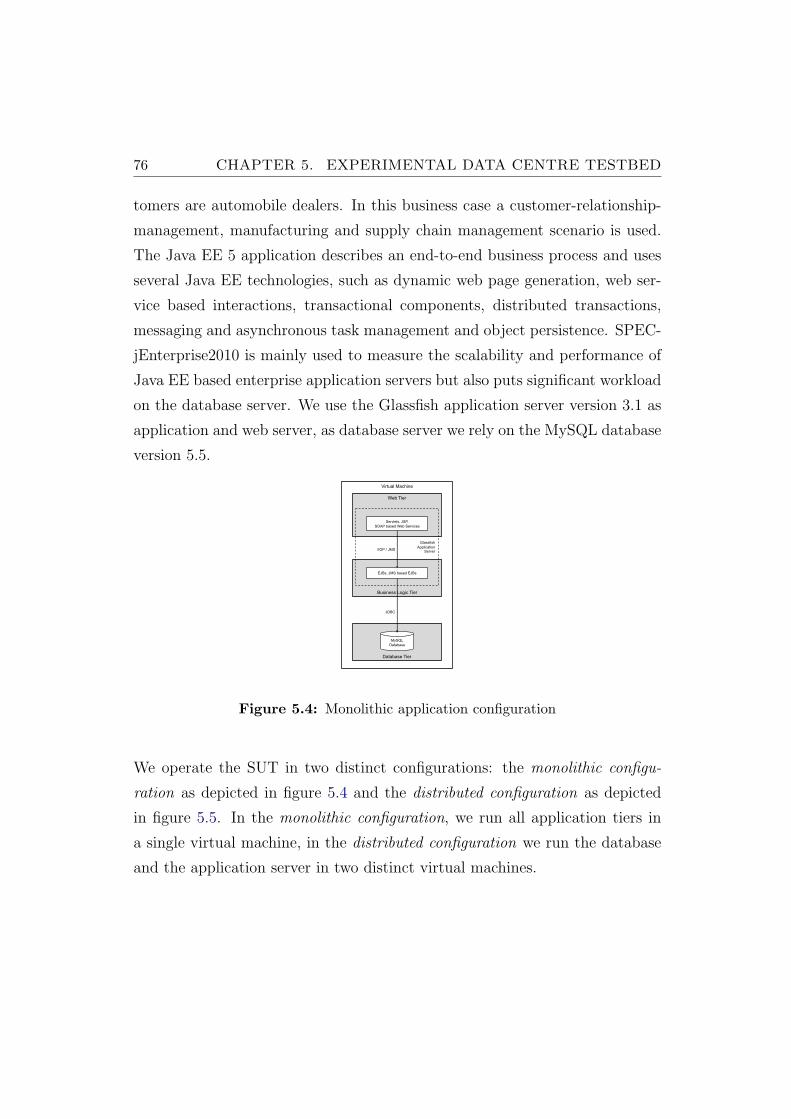
76 CHAPTER 5. EXPERIMENTAL DATA CENTRE TESTBED
tomers are automobile dealers. In this business case a customer-relationship-
management, manufacturing and supply chain management scenario is used.
The Java EE 5 application describes an end-to-end business process and uses
several Java EE technologies, such as dynamic web page generation, web ser-
vice based interactions, transactional components, distributed transactions,
messaging and asynchronous task management and object persistence. SPEC-
jEnterprise2010 is mainly used to measure the scalability and performance of
Java EE based enterprise application servers but also puts significant workload
on the database server. We use the Glassfish application server version 3.1 as
application and web server, as database server we rely on the MySQL database
version 5.5.
!""#$%&$'()*+,)$
Virtual Machine
Virtual Machine
-.$
Database Tier
Business Logic Tier
Web Tier
MySQL
Database
Glassfish
Application Server
EJBs, JMS based EJBs
Servlets, JSP,
SOAP based Web Services
JDBC
IIOP / JMS
Virtual Machine
Database Tier
Business Logic Tier
Web Tier
MySQL
Database
Glassfish
Application Server
EJBs, JMS based EJBs
Servlets, JSP,
SOAP based Web Services
JDBC
IIOP / JMS
Figure 5.4: Monolithic application configuration
We operate the SUT in two distinct configurations: the monolithic configu-
ration as depicted in figure 5.4 and the distributed configuration as depicted
in figure 5.5. In the monolithic configuration, we run all application tiers in
a single virtual machine, in the distributed configuration we run the database
and the application server in two distinct virtual machines.
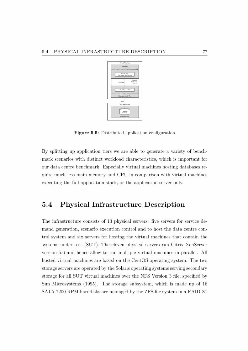
5.4. PHYSICAL INFRASTRUCTURE DESCRIPTION 77
!""#$%&$'()*+,)$
Virtual Machine
Virtual Machine
-.$
Database Tier
Business Logic Tier
Web Tier
MySQL
Database
Glassfish
Application Server
EJBs, JMS based EJBs
Servlets, JSP,
SOAP based Web Services
JDBC
IIOP / JMS
Virtual Machine
Database Tier
Business Logic Tier
Web Tier
MySQL
Database
Glassfish
Application Server
EJBs, JMS based EJBs
Servlets, JSP,
SOAP based Web Services
JDBC
IIOP / JMS
Figure 5.5: Distributed application configuration
By splitting up application tiers we are able to generate a variety of bench-
mark scenarios with distinct workload characteristics, which is important for
our data centre benchmark. Especially virtual machines hosting databases re-
quire much less main memory and CPU in comparison with virtual machines
executing the full application stack, or the application server only.
5.4 Physical Infrastructure Description
The infrastructure consists of 13 physical servers: five servers for service de-
mand generation, scenario execution control and to host the data centre con-
trol system and six servers for hosting the virtual machines that contain the
systems under test (SUT). The eleven physical servers run Citrix XenServer
version 5.6 and hence allow to run multiple virtual machines in parallel. All
hosted virtual machines are based on the CentOS operating system. The two
storage servers are operated by the Solaris operating systems serving secondary
storage for all SUT virtual machines over the NFS Version 3 file, specified by
Sun Microsystems (1995). The storage subsystem, which is made up of 16
SATA 7200 RPM harddisks are managed by the ZFS file system in a RAID-Z1

78 CHAPTER 5. EXPERIMENTAL DATA CENTRE TESTBED
assemblage. All NFS shares are network accessible over a channel bond of two
1 G/bit ethernet interfaces. The bond implements data striping to achieve
higher throughput by data aggregation over multiple network links simulta-
neously. The switch is configured for bonding assistance. The SUT physical
servers use a dedicated bond of two 1 G/bit ethernet interfaces for traffic tar-
geting at the storage servers. A single 1 G/bit ethernet interface is reserved for
virtual machine live migrations and resource monitoring and a fourth 1 G/bit
ethernet interface is dedicated for network traffic that is targeted to the SUT
systems. The three types of network traffic are well separated and sufficiently
capacitated to prevent any network bottlenecks.
5.4.1 Physical Server Configuration
The SUT physical servers are equipped with one Intel Nehalem Xeon E5520
CPU with 4 cores, 16 GB main memory and four 1 Gbit Ethernet network
interfaces. Each core owns a private L1 and L2 cache, the 8 MB L3-Cache is
shared amongst all cores. Each processor core features an integrated Quick-
Path Interconnect memory controller.
!""#$%&$'()*+,)$ -.$
Main Memory
Chip
Cache
Core 1 Core 2
Cache Cache
Main Memory
Chip
Cache
Core 1
Cache
Thread 1 Thread 2
Figure 5.6: Hardware setup, two hyper-threads, one CPU core
We operated the physical servers with only one core activated, but hyper-
threading activated, leading to two logical processors or hyper-threads on the
5.4. PHYSICAL INFRASTRUCTURE DESCRIPTION 79
active physical core. Each individual hyper-thread is abstracted by the hard-
ware as a logical processors and is presented to the hypervisor as a physical
processor. The two hyper-threads share the cache-hierachy of the physical
core. The configuration is depicted in figure 5.6. We will refer to this setup as
the hyper-threaded hardware setup.
5.4.2 Intel’s Hyper-Threading Technology
The Intel ”Hyper-Threading Technology” (Intel, 2012) is an implementation of
simultaneous multithreading. It allows multiple threads to execute in parallel,
that is, instructions from multiple application threads can be executed within a
single hardware cycle. In contrast to other multithreading models described by
Tullsen et al. (1998), all hardware contexts are simultaneously active, thereby
competing for all processor resources. The availability of a larger numbers of
instructions scheduled for execution potentially increases the per cycle as well
as overall utilization of the processor because of increased instruction-level
parallelism and interference effects. At the same time, as a single physical
processor or core is able to execute two or more threads at the same time,
hardware resources are fully shared, in particular hardware caches, which is a
cause for thread interference effects as shown by Tam et al. (2007), Chandra
et al. (2005) and Iyer (2004). Shared last level caches (L3) may lead to a
removal of parts or even the full memory working set of an operating system
thread, let alone a virtual machine. The result is performance degradation or
variability for threads or virtual machines. The level of variability then depends
on which other virtual machines and what type of workloads are concurrently
running on the other hyper-thread. For hyper-threads sharing not only the
last level but the full cache hierarchy, the performance variability may even
be higher in contrast to physical cores sharing the L3 cache only. According
to Nathuji et al. (2010), technologies like hyper-threading designed to increase
resource efficiency almost unavoidably lead to increases in interference and
80 CHAPTER 5. EXPERIMENTAL DATA CENTRE TESTBED
contention for hardware resources.
For operating systems, awareness of the processor hierarchy is desirable in
order to avoid circumstances such as a system with two physical cores hav-
ing two runnable threads scheduled on two hyper-threads of one core and
therefore sharing resources while the remaining physical core is idle. Current
operating systems have this kind of awareness built in. We are not aware
of any processor hierarchy awareness in the Xen CPU scheduler. In Xen, an
administrator may use the possibility to pin virtual CPUs to logical proces-
sors in a hierarchy-aware way. However, a statical assignment may lead to
asymmetric and unfair resource allocation as a core with all hyper-threads idle
provides more CPU resources than a core with only one idle hyper-thread and
all other hyper-threads busy. VMWare’s hypervisor (VMWare, 2012b) pre-
vents this issue as the CPU scheduler can be configured to control the way
hyper-threads are utilized by charging consumed CPU time only partially if a
virtual CPU is scheduled on a hyper-thread. For operating systems, Bulpin
and Pratt (2005) show that the CPU scheduler can improve application level
throughput by scheduling application threads in parallel on hyper-threads of
a core that deliver combined throughput better than other application level
thread combinations. To achieve throughput improvement, processor metrics
are used to inform the scheduler of the realized performance. Since hyper-
threads share a physical core, they run slower than they would do if they had
exclusive use of a core. However, in most cases the combined throughput of
the threads is higher than the throughput of either one of them running ex-
clusively, providing increased throughput at the expense of individual threads’
throughput. According to Tuck and Tullsen (2003) and Bulpin and Pratt
(2004), the overall system throughput can be expected to increase for about
20% using hyper-threading. Despite these findings, it is also known that there
exist combinations of workloads that reduce throughput or lead to a biased
per-thread throughput.
The possible increases in throughput and the possibility to co-schedule do-
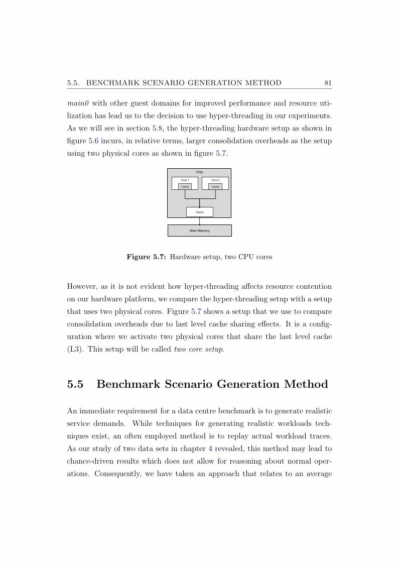
5.5. BENCHMARK SCENARIO GENERATION METHOD 81
main0 with other guest domains for improved performance and resource uti-
lization has lead us to the decision to use hyper-threading in our experiments.
As we will see in section 5.8, the hyper-threading hardware setup as shown in
figure 5.6 incurs, in relative terms, larger consolidation overheads as the setup
using two physical cores as shown in figure 5.7.
!""#$%&$'()*+,)$ -.$
Main Memory
Chip
Cache
Core 1 Core 2
Cache Cache
Main Memory
Chip
Cache
Core 1
Cache
Thread 1 Thread 2
Figure 5.7: Hardware setup, two CPU cores
However, as it is not evident how hyper-threading affects resource contention
on our hardware platform, we compare the hyper-threading setup with a setup
that uses two physical cores. Figure 5.7 shows a setup that we use to compare
consolidation overheads due to last level cache sharing effects. It is a config-
uration where we activate two physical cores that share the last level cache
(L3). This setup will be called two core setup.
5.5 Benchmark Scenario Generation Method
An immediate requirement for a data centre benchmark is to generate realistic
service demands. While techniques for generating realistic workloads tech-
niques exist, an often employed method is to replay actual workload traces.
As our study of two data sets in chapter 4 revealed, this method may lead to
chance-driven results which does not allow for reasoning about normal oper-
ations. Consequently, we have taken an approach that relates to an average
82 CHAPTER 5. EXPERIMENTAL DATA CENTRE TESTBED
analysis by generating workloads that replay typical workload patterns rather
than replaying random and possibly outlier afflicted instantiations of the pat-
terns. In this respect, our approach differs from others that have been pro-
posed for studying web based application performance, content distribution,
load balancing, caching or resource allocation. The work of Urgaonkar and
Shenoy (2008), Welsh and Culler (2003), Urgaonkar et al. (2008) or Chen and
Heidemann (2002) put a primary focus on how systems perform under steady
workload increases, sudden workload spikes or flash crowds, that present excep-
tional situations. While it is interesting how unforeseen service demand spikes
can be handled and according to Bodik et al. (2009) as stochastic service de-
mand for web based applications is much more the rule than the exception for
large, public web sites, our focus is on enterprise applications for which service
demand is much more stable and predictable. For enterprise environments, we
undertake the first attempt for the definition of a data centre benchmark.
The statistical analysis in subsection 4.1.2 revealed that service demand for the
processes in our data set exhibit regular daily and weekly demand patterns with
sharp outliers leading to large peak to mean ratios and rather extreme levels
of volatility. In our study, we are interested in exploring normal operations
rather than exceptional situations that are hard to predict and may require
admission control and load balancing to ensure application performance. We
focus on daily patterns that recur on working days and derive service demands
that represent demand profiles that do not exhibit exceptionally high service
demand levels. Due to time constraints for our study, a benchmark scenario
is executed in 12 hours real time, simulating 24 hours of operations.
A benchmark scenario consists of a set of virtual machines with resource de-
mand profiles that can be consolidated, using the overhead aware static server
consolidation model described in section 3.3 with 24 time intervals onto six
physical servers. We can control the amount, the type and the relative ca-
pacity of the virtual machines during the scenario generation process. The
resource requirements of the virtual machines are determined during the ser-
5.5. BENCHMARK SCENARIO GENERATION METHOD 83
vice demand generation process for each SUT. Each SUT’s service demand is
derived from a randomly drawn process of the service demand trace data set.
Duplicates are allowed, however as different demand levels are assigned to the
SUTs, the general demand pattern may be the same but the demand intensity
will be different.
Once a service demand trace is assigned to each virtual machine running a web
and application server in a scenario, the actual service demand is generated in
the following way:
1. Normalize each service trace using its maximum value: we are interested
in the general demand pattern, not the actual demand intensity. The
intensity is rather specific to our data set.
2. For each virtual machine j ∈ J , generate the service demand distribu-
tions Xstj for each hour of a day (t ∈ T , |T | = 24). The resulting, per
hour demand distribution for an example process is shown in figure 5.8.
3. Filter the distribution by removing all values above the 75 % percentile
and below the 25 % percentile of Xstj, leading to the truncated service
demand distribution Y stj = {x ∈ Xs
tj | x ≥ Q0.25(Xtj) ∨ x ≤ Q0.75(Xtj)}
4. The median of the truncated distribution is used to define the service
demand level series ~lsj at each time interval t ∈ T : lstj = Q0.50(Y sti). The
median is shown in figure 5.8 by the solid red line.
5. The 95 % percentile of the truncated distributions is used to define
the planned service demand level P sti at each time period t ∈ T :
P sti = Q0.95(Y s
ti). This demand level is used to estimate the CPU de-
mands in each time interval using a lookup table. The table stores CPU
demand estimates obtained in offline measurements: for each amount of
virtual users {10, 20, 30...200} the CPU demand level is given. The de-
mand level is the average of three measurement runs plus two times the
84 CHAPTER 5. EXPERIMENTAL DATA CENTRE TESTBED
standard deviation. We have chosen this simple estimation procedure
as it ensures sufficient resources and service level preserving application
response times.
6. Each entry lsti defines the demand level for period t ∈ T and is the equiv-
alent to the CPU demand estimate ajtr used for consolidation planning
in the server consolidation models presented in chapter 3. As it is unre-
alistic to assume a steady service demand level for the duration of half
an hour, we expand the series ~lsi by replacing each entry lsti with repeat-
ing it 30 times, leading to 720 entries in the time series ~lsi . Each entry
corresponds to the service demand level of a minute real time (or two
minutes simulated time). Padala et al. (2009) even change the amount
of virtual users every 10 seconds to generate a realistic service demand
that matches the characteristics of production traces.
7. ~lsi is a step function of time t ∈ T . As a series contains very sharp in- and
decreases in service demand values, we smooth the series using a simple
moving average filter with a sliding window length of 6 values. We will
denote the smoothed series with ~lsi .
8. The series ~lsi is very smooth and still far from generating resource de-
mands as volatile as we could observe in the resource demand data set.
We add noise to each value of ~lsi according to the variance we have found
in the truncated service demand distribution Y sti for the corresponding
hour of the day. For this purpose we define a random variable Zsti that
follows a normal distribution N(0, σ(Y sti)). Each value of ~lsi is replaced
by adding a randomly drawn value from N(0, σ(Y sti)). However, we do
not exceed the value Q0.75(Xtj) which avoids large outliers.
9. We normalize the series ~lsi again to its new maximum value. This allows
us to assign a maximum service demand to a series in a subsequent step
and to plan for the maximum resource demands of a virtual machine.
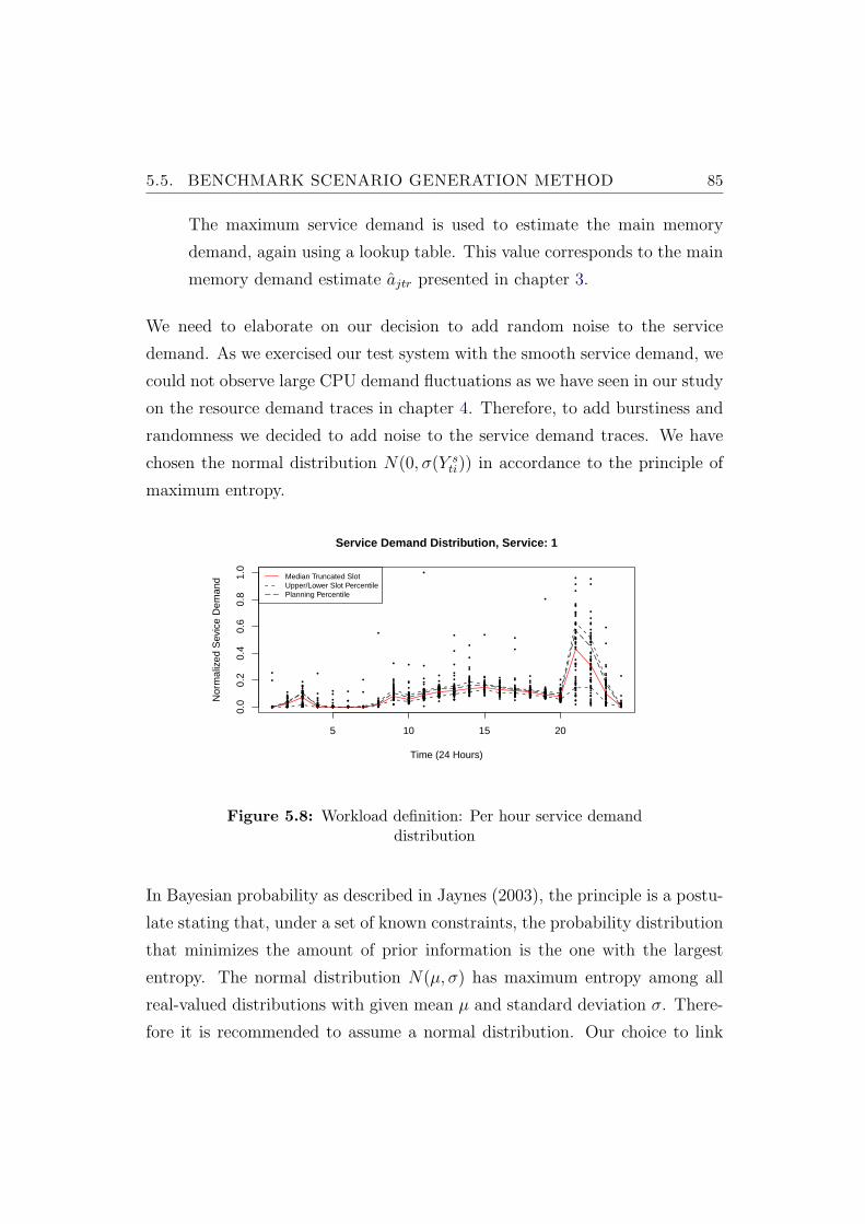
5.5. BENCHMARK SCENARIO GENERATION METHOD 85
The maximum service demand is used to estimate the main memory
demand, again using a lookup table. This value corresponds to the main
memory demand estimate ajtr presented in chapter 3.
We need to elaborate on our decision to add random noise to the service
demand. As we exercised our test system with the smooth service demand, we
could not observe large CPU demand fluctuations as we have seen in our study
on the resource demand traces in chapter 4. Therefore, to add burstiness and
randomness we decided to add noise to the service demand traces. We have
chosen the normal distribution N(0, σ(Y sti)) in accordance to the principle of
maximum entropy.
●●
●
●
●●●●●●●●●●●●●●●●●●●●●●●●●●●●●●●●●●●●●●●●●●●●●●●●●●●
●
●
●
●●
●
●
●
●●
●
●
●
●
●
●●●
●●
●
●
●
●●
●
●
●●
●
●
●
●
●
●
●●●●●
●
●
●
●●
●
●●
●●
●●
●
●
●
●
●
●
●
●
●
●
●
●
●
●●●
●
●
●
●
●
●
●
●
●●
●
●
●
●●
●●
●
●
●
●
●
●
●●
●●
●
●
●
●●
●
●●
●
●
●
●●
●
●
●
●
●
●
●●●
●
●●●●●
●
●
●●●●●●
●
●
●●●
●
●●●●
●●
●●●●●●●●●●●●●●●●●●
●
●
●
● ●●●●●●●●●●●●●
●
●●●●
●
●●●●
●
●●●●●●●●●●●●●●●●●
●
●●●●●●●●●●●
●
● ●●●●●●●●●●●●●●●●●●
●
●●●●●●●●●●●●●●●●●●●●●●
●
●●●●●●
●
●●●●●● ●●●●●●●●●●●●●●●●
●
●●●●●●●●●●●●●●●●●●●●●●●●
●
●●●●●●●●●●●●●●●●●●●●
●
●●●
●●
●●
●
●
●●●●
●●
●
●●
●
●●●
●
●●●
●●●●●●
●
●
●●
●
●●
●
●
●
●
●
●
●
●
●
●
●●●
●
●●●
●
●
●
●
●
●●
●●
●
●
●
●
●
●
●
●●
●
●
●
●
●
●
●
●
●●
●
●
●
●
●
●
●
●
●
●●
●
●
●
●
●
●
●
●
●
●
●
●●
●
●
●●
●
●
●
●
●
●
●
●
●
●
●
●●
●
●
●
●
●
●
●●●●●●
●
●
●
●●
●
●
●
●
●
●
●●●
●
●
●
●
●
●
●
●
●
●
●
●
●
●●
●●
●
●
●
●
●●
●
●●
●
●●
●
●
●
●
●●
●
●
●
●●●
●
●
●●
●●
●
●
●●
●
●●●
●
●
●●
●
●
●●
●
●
●
●
●
●
●
●
●
●
●
●
●
●●
●
●
●
●●
●●
●
●
●
●●
●●
●●
●
●
●
●
●
●
●
●
●
●
●
●
●
●●
●
●
●
●●●
●
●
●
●●
●●
●
●
●
●
●
●
●
●
●
●
●
●
●
●
●
●
●
●
●●
●
●
●
●
●
●
●
●●
●
●
●
●
●
●
●
●
●
●
●
●●
●●
●
●●●
●
●
●
●
●
●●
●
●
●
●
●
●
●
●
●
●
●
●
●
●
●
●
●
●
●
●
●●
●
●
●
●
●●
●
●
●
●●●●
●
●
●
●●
●
●
●●
●
●●
●
●●
●
●
●
●
●
●
●●●●
●
●
●●
●●
●
●
●
●
●
●
●
●
●
●●
●
●
●
●
●
●
●
●
●
●
●
●
●
●
●
●●
●●
●
●●
●
●
●
●
●
●
●
●
●
●
●
●
●
●
●
●
●
●
●
●●
●
●
●●
●
●
●
●
●●
●
●
●
●
●
●
●
●
●
●
●●●
●
●
●●
●
●
●
●
●
●
●
●●
●
●
●
●
●●●●●
●
●
●
●
●
●
●
●
●●●
●●●
●
●
●
●
●
●●
●●
●
●
●
●
●●●
●●
●
●
●
●
●
●
●
●
●
●●
●
●●
●
●
●
●
●
●
●
●
●
●
●
●●●
●
●●
●●
●
●
●
●
●
●
●
●
●●
●
●●
●
●
●
●●
●
●●●●●
●
●
●
●
●●
●
●
●
●
●
●●●
●
●
●
●
●
●●
●
●
●●
●
●
●
●
●
●●
●
●
●
●
●
●
●●
●
●●
●
●
●
●
●
●●●
●●●
●●
●
●
●
●
●
●●
●
●
●
●
●●
●
●
●
●
●●
●●
●
●
●●
●
●
●
●
●
●●●
●
●
●
●
●●
●
●
●
●
●
●
●●
●●
●
●
●
●●
●
●
●
●●●
●
●●
●●●
●
●
●
●
●
●
●
●
●
●
●
●
●
●
●
●
●
●
●
●
●
●
●
●
●
●
●
●
●
●
●
●
●
●
●
●
●
●
●
●
●
●
●
●
●
●
●
●
●
●
●
●
●
●
●
●
●
●
●
●
●
●
●
●
●
●
●
●
●
●
●
●
●
●
●
●
●
●
●
●
●
●
●
●
●
●
●
●
●
●
●
●
●
●
●
●
●
●
●
●
●
●
●
●
●
●
●
●
●
●
●
●
●
●
●●●
●
●
●
●●
●
●
●
●
●
●
●
●
●
●
●
●
●
●
●
●
●
●
●
●●
●
●
●
●
●
●
●
●
●
●●
●
●
●
●
●
●
●
●
●
●●
●
●●
●
●
●
●
●
●
●
●
●●●●●●●●
●●●
●
●
●●●●
●
●●●●●●●●●●●●●●●
●
●●
●●●●●●●●●●●
5 10 15 20
0.0
0.2
0.4
0.6
0.8
1.0
Service Demand Distribution, Service: 1
Time (24 Hours)
Nor
mal
ized
Sev
ice
Dem
and Median Truncated Slot
Upper/Lower Slot PercentilePlanning Percentile
Figure 5.8: Workload definition: Per hour service demanddistribution
In Bayesian probability as described in Jaynes (2003), the principle is a postu-
late stating that, under a set of known constraints, the probability distribution
that minimizes the amount of prior information is the one with the largest
entropy. The normal distribution N(µ, σ) has maximum entropy among all
real-valued distributions with given mean µ and standard deviation σ. There-
fore it is recommended to assume a normal distribution. Our choice to link
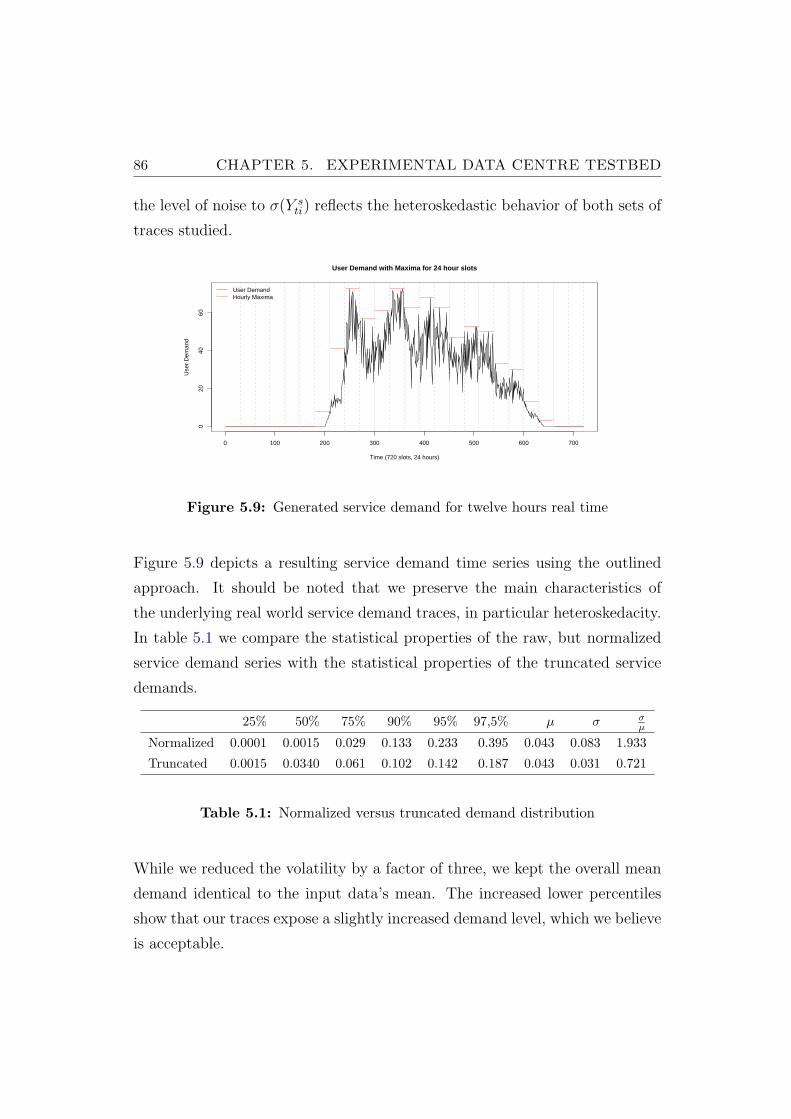
86 CHAPTER 5. EXPERIMENTAL DATA CENTRE TESTBED
the level of noise to σ(Y sti) reflects the heteroskedastic behavior of both sets of
traces studied.
User Demand with Maxima for 24 hour slots
Time (720 slots, 24 hours)
Use
r D
eman
d
0 100 200 300 400 500 600 700
020
4060
User DemandHourly Maxima
Figure 5.9: Generated service demand for twelve hours real time
Figure 5.9 depicts a resulting service demand time series using the outlined
approach. It should be noted that we preserve the main characteristics of
the underlying real world service demand traces, in particular heteroskedacity.
In table 5.1 we compare the statistical properties of the raw, but normalized
service demand series with the statistical properties of the truncated service
demands.
25% 50% 75% 90% 95% 97,5% µ σ σµ
Normalized 0.0001 0.0015 0.029 0.133 0.233 0.395 0.043 0.083 1.933
Truncated 0.0015 0.0340 0.061 0.102 0.142 0.187 0.043 0.031 0.721
Table 5.1: Normalized versus truncated demand distribution
While we reduced the volatility by a factor of three, we kept the overall mean
demand identical to the input data’s mean. The increased lower percentiles
show that our traces expose a slightly increased demand level, which we believe
is acceptable.
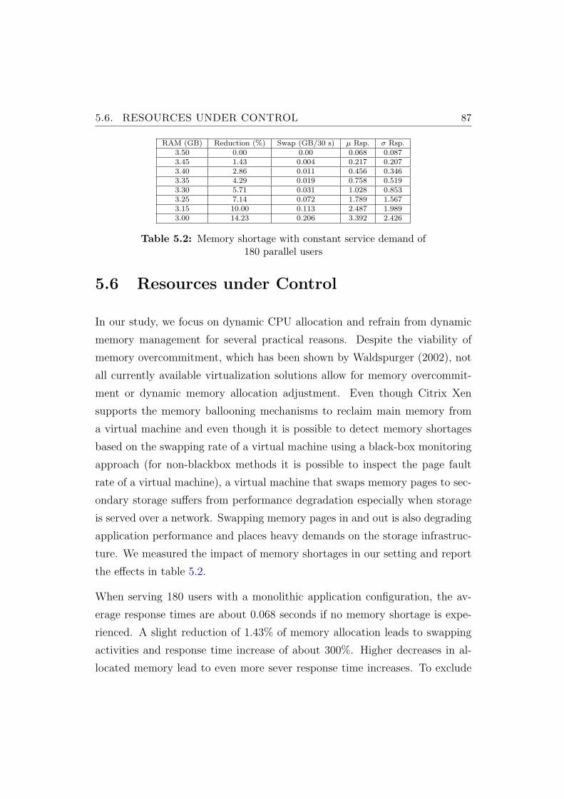
5.6. RESOURCES UNDER CONTROL 87
RAM (GB) Reduction (%) Swap (GB/30 s) µ Rsp. σ Rsp.3.50 0.00 0.00 0.068 0.0873.45 1.43 0.004 0.217 0.2073.40 2.86 0.011 0.456 0.3463.35 4.29 0.019 0.758 0.5193.30 5.71 0.031 1.028 0.8533.25 7.14 0.072 1.789 1.5673.15 10.00 0.113 2.487 1.9893.00 14.23 0.206 3.392 2.426
Table 5.2: Memory shortage with constant service demand of180 parallel users
5.6 Resources under Control
In our study, we focus on dynamic CPU allocation and refrain from dynamic
memory management for several practical reasons. Despite the viability of
memory overcommitment, which has been shown by Waldspurger (2002), not
all currently available virtualization solutions allow for memory overcommit-
ment or dynamic memory allocation adjustment. Even though Citrix Xen
supports the memory ballooning mechanisms to reclaim main memory from
a virtual machine and even though it is possible to detect memory shortages
based on the swapping rate of a virtual machine using a black-box monitoring
approach (for non-blackbox methods it is possible to inspect the page fault
rate of a virtual machine), a virtual machine that swaps memory pages to sec-
ondary storage suffers from performance degradation especially when storage
is served over a network. Swapping memory pages in and out is also degrading
application performance and places heavy demands on the storage infrastruc-
ture. We measured the impact of memory shortages in our setting and report
the effects in table 5.2.
When serving 180 users with a monolithic application configuration, the av-
erage response times are about 0.068 seconds if no memory shortage is expe-
rienced. A slight reduction of 1.43% of memory allocation leads to swapping
activities and response time increase of about 300%. Higher decreases in al-
located memory lead to even more sever response time increases. To exclude
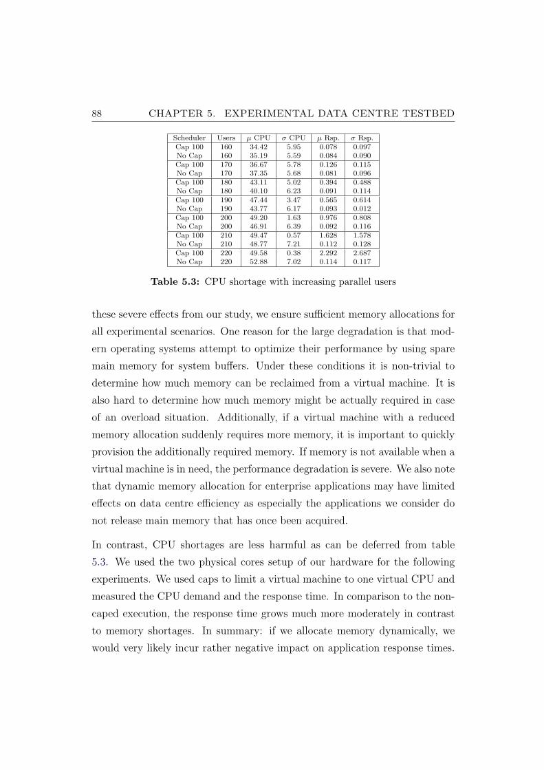
88 CHAPTER 5. EXPERIMENTAL DATA CENTRE TESTBED
Scheduler Users µ CPU σ CPU µ Rsp. σ Rsp.Cap 100 160 34.42 5.95 0.078 0.097No Cap 160 35.19 5.59 0.084 0.090Cap 100 170 36.67 5.78 0.126 0.115No Cap 170 37.35 5.68 0.081 0.096Cap 100 180 43.11 5.02 0.394 0.488No Cap 180 40.10 6.23 0.091 0.114Cap 100 190 47.44 3.47 0.565 0.614No Cap 190 43.77 6.17 0.093 0.012Cap 100 200 49.20 1.63 0.976 0.808No Cap 200 46.91 6.39 0.092 0.116Cap 100 210 49.47 0.57 1.628 1.578No Cap 210 48.77 7.21 0.112 0.128Cap 100 220 49.58 0.38 2.292 2.687No Cap 220 52.88 7.02 0.114 0.117
Table 5.3: CPU shortage with increasing parallel users
these severe effects from our study, we ensure sufficient memory allocations for
all experimental scenarios. One reason for the large degradation is that mod-
ern operating systems attempt to optimize their performance by using spare
main memory for system buffers. Under these conditions it is non-trivial to
determine how much memory can be reclaimed from a virtual machine. It is
also hard to determine how much memory might be actually required in case
of an overload situation. Additionally, if a virtual machine with a reduced
memory allocation suddenly requires more memory, it is important to quickly
provision the additionally required memory. If memory is not available when a
virtual machine is in need, the performance degradation is severe. We also note
that dynamic memory allocation for enterprise applications may have limited
effects on data centre efficiency as especially the applications we consider do
not release main memory that has once been acquired.
In contrast, CPU shortages are less harmful as can be deferred from table
5.3. We used the two physical cores setup of our hardware for the following
experiments. We used caps to limit a virtual machine to one virtual CPU and
measured the CPU demand and the response time. In comparison to the non-
caped execution, the response time grows much more moderately in contrast
to memory shortages. In summary: if we allocate memory dynamically, we
would very likely incur rather negative impact on application response times.
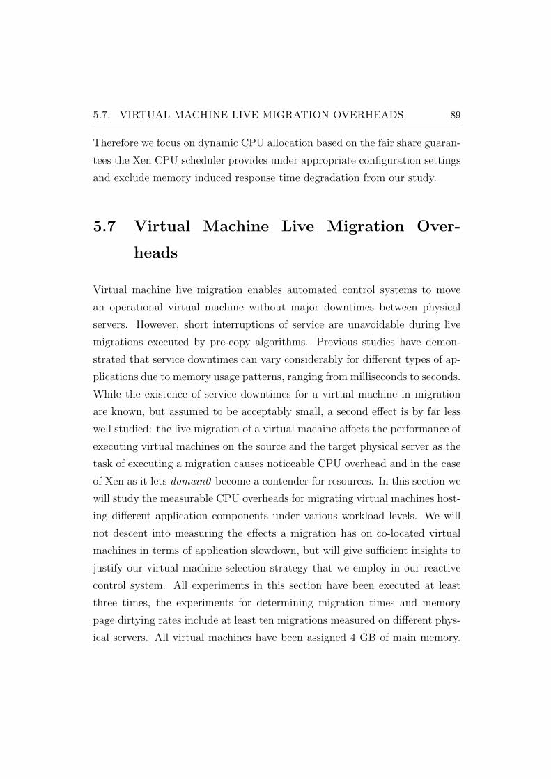
5.7. VIRTUAL MACHINE LIVE MIGRATION OVERHEADS 89
Therefore we focus on dynamic CPU allocation based on the fair share guaran-
tees the Xen CPU scheduler provides under appropriate configuration settings
and exclude memory induced response time degradation from our study.
5.7 Virtual Machine Live Migration Over-
heads
Virtual machine live migration enables automated control systems to move
an operational virtual machine without major downtimes between physical
servers. However, short interruptions of service are unavoidable during live
migrations executed by pre-copy algorithms. Previous studies have demon-
strated that service downtimes can vary considerably for different types of ap-
plications due to memory usage patterns, ranging from milliseconds to seconds.
While the existence of service downtimes for a virtual machine in migration
are known, but assumed to be acceptably small, a second effect is by far less
well studied: the live migration of a virtual machine affects the performance of
executing virtual machines on the source and the target physical server as the
task of executing a migration causes noticeable CPU overhead and in the case
of Xen as it lets domain0 become a contender for resources. In this section we
will study the measurable CPU overheads for migrating virtual machines host-
ing different application components under various workload levels. We will
not descent into measuring the effects a migration has on co-located virtual
machines in terms of application slowdown, but will give sufficient insights to
justify our virtual machine selection strategy that we employ in our reactive
control system. All experiments in this section have been executed at least
three times, the experiments for determining migration times and memory
page dirtying rates include at least ten migrations measured on different phys-
ical servers. All virtual machines have been assigned 4 GB of main memory.
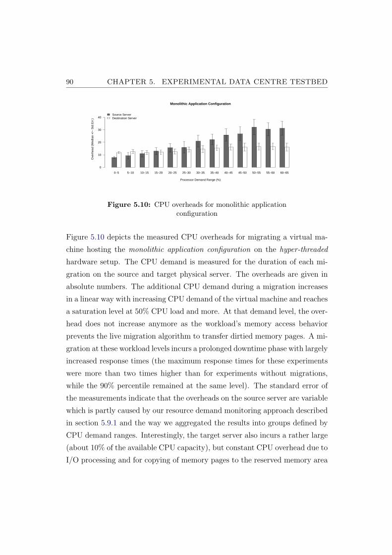
90 CHAPTER 5. EXPERIMENTAL DATA CENTRE TESTBED
0−5 5−10 10−15 15−20 20−25 25−30 30−35 35−40 40−45 45−50 50−55 55−60 60−65
Monolithic Application Configuration
Processor Demand Range (%)
Ove
rhea
d (M
edia
n +
/− S
td.E
rr.)
0
10
20
30
40Source ServerDestination Server
Figure 5.10: CPU overheads for monolithic applicationconfiguration
Figure 5.10 depicts the measured CPU overheads for migrating a virtual ma-
chine hosting the monolithic application configuration on the hyper-threaded
hardware setup. The CPU demand is measured for the duration of each mi-
gration on the source and target physical server. The overheads are given in
absolute numbers. The additional CPU demand during a migration increases
in a linear way with increasing CPU demand of the virtual machine and reaches
a saturation level at 50% CPU load and more. At that demand level, the over-
head does not increase anymore as the workload’s memory access behavior
prevents the live migration algorithm to transfer dirtied memory pages. A mi-
gration at these workload levels incurs a prolonged downtime phase with largely
increased response times (the maximum response times for these experiments
were more than two times higher than for experiments without migrations,
while the 90% percentile remained at the same level). The standard error of
the measurements indicate that the overheads on the source server are variable
which is partly caused by our resource demand monitoring approach described
in section 5.9.1 and the way we aggregated the results into groups defined by
CPU demand ranges. Interestingly, the target server also incurs a rather large
(about 10% of the available CPU capacity), but constant CPU overhead due to
I/O processing and for copying of memory pages to the reserved memory area
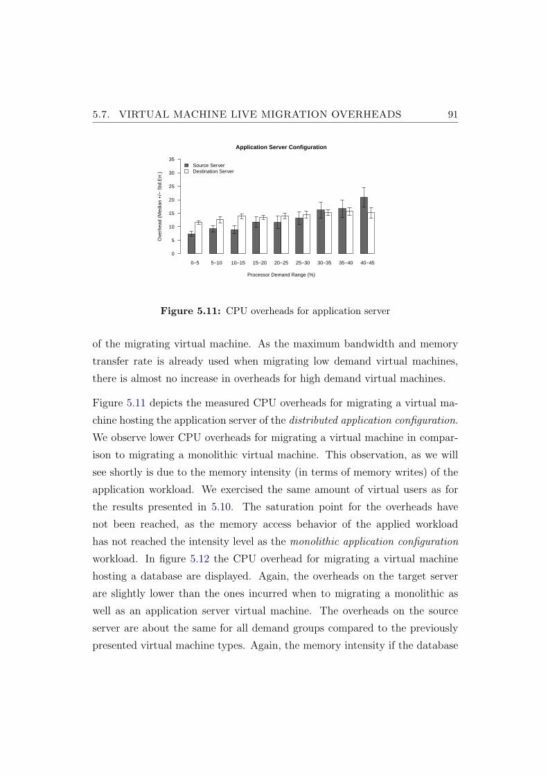
5.7. VIRTUAL MACHINE LIVE MIGRATION OVERHEADS 91
0−5 5−10 10−15 15−20 20−25 25−30 30−35 35−40 40−45
Application Server Configuration
Processor Demand Range (%)
Ove
rhea
d (M
edia
n +
/− S
td.E
rr.)
0
5
10
15
20
25
30
35Source ServerDestination Server
Figure 5.11: CPU overheads for application server
of the migrating virtual machine. As the maximum bandwidth and memory
transfer rate is already used when migrating low demand virtual machines,
there is almost no increase in overheads for high demand virtual machines.
Figure 5.11 depicts the measured CPU overheads for migrating a virtual ma-
chine hosting the application server of the distributed application configuration.
We observe lower CPU overheads for migrating a virtual machine in compar-
ison to migrating a monolithic virtual machine. This observation, as we will
see shortly is due to the memory intensity (in terms of memory writes) of the
application workload. We exercised the same amount of virtual users as for
the results presented in 5.10. The saturation point for the overheads have
not been reached, as the memory access behavior of the applied workload
has not reached the intensity level as the monolithic application configuration
workload. In figure 5.12 the CPU overhead for migrating a virtual machine
hosting a database are displayed. Again, the overheads on the target server
are slightly lower than the ones incurred when to migrating a monolithic as
well as an application server virtual machine. The overheads on the source
server are about the same for all demand groups compared to the previously
presented virtual machine types. Again, the memory intensity if the database
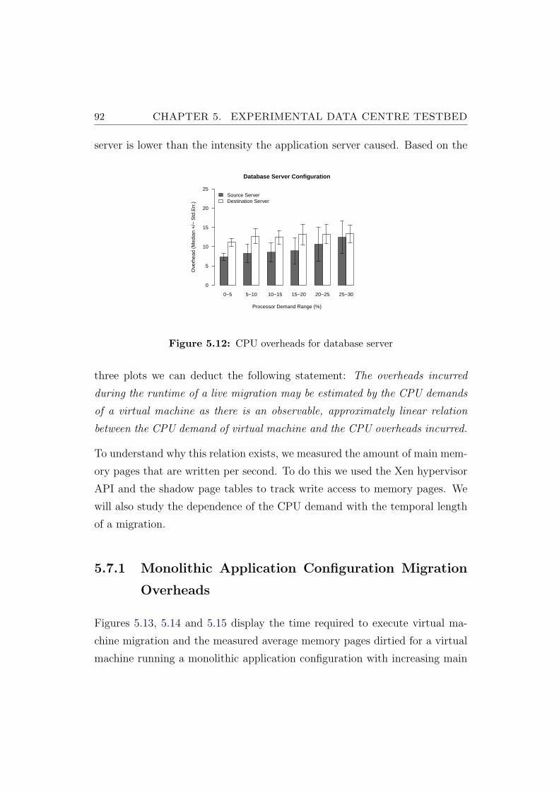
92 CHAPTER 5. EXPERIMENTAL DATA CENTRE TESTBED
server is lower than the intensity the application server caused. Based on the
0−5 5−10 10−15 15−20 20−25 25−30
Database Server Configuration
Processor Demand Range (%)
Ove
rhea
d (M
edia
n +
/− S
td.E
rr.)
0
5
10
15
20
25Source ServerDestination Server
Figure 5.12: CPU overheads for database server
three plots we can deduct the following statement: The overheads incurred
during the runtime of a live migration may be estimated by the CPU demands
of a virtual machine as there is an observable, approximately linear relation
between the CPU demand of virtual machine and the CPU overheads incurred.
To understand why this relation exists, we measured the amount of main mem-
ory pages that are written per second. To do this we used the Xen hypervisor
API and the shadow page tables to track write access to memory pages. We
will also study the dependence of the CPU demand with the temporal length
of a migration.
5.7.1 Monolithic Application Configuration Migration
Overheads
Figures 5.13, 5.14 and 5.15 display the time required to execute virtual ma-
chine migration and the measured average memory pages dirtied for a virtual
machine running a monolithic application configuration with increasing main
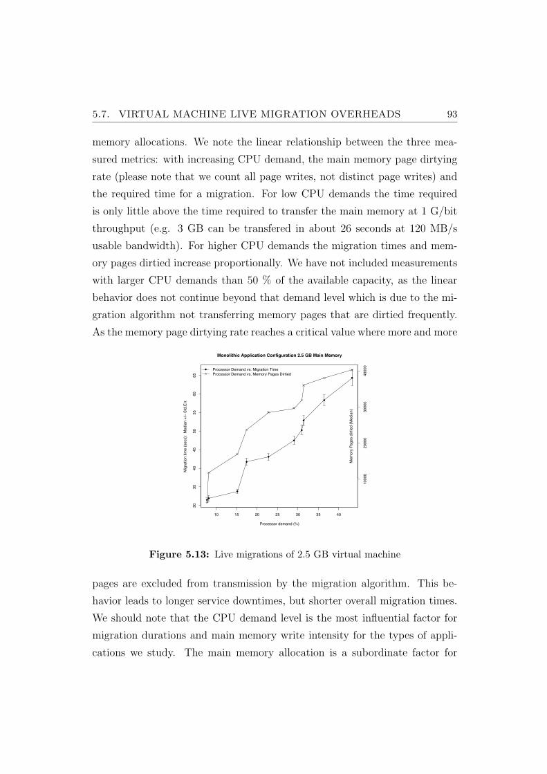
5.7. VIRTUAL MACHINE LIVE MIGRATION OVERHEADS 93
memory allocations. We note the linear relationship between the three mea-
sured metrics: with increasing CPU demand, the main memory page dirtying
rate (please note that we count all page writes, not distinct page writes) and
the required time for a migration. For low CPU demands the time required
is only little above the time required to transfer the main memory at 1 G/bit
throughput (e.g. 3 GB can be transfered in about 26 seconds at 120 MB/s
usable bandwidth). For higher CPU demands the migration times and mem-
ory pages dirtied increase proportionally. We have not included measurements
with larger CPU demands than 50 % of the available capacity, as the linear
behavior does not continue beyond that demand level which is due to the mi-
gration algorithm not transferring memory pages that are dirtied frequently.
As the memory page dirtying rate reaches a critical value where more and more
!!
!
!
!
!
!
!
!
!
10 15 20 25 30 35 40
30
35
40
45
50
55
60
65
Processor demand (%)
Mig
ratio
n t
ime
(se
cs):
M
ed
ian
+/!
Std
.Err
.
Monolithic Application Configuration 2.5 GB Main Memory
10
00
02
00
00
30
00
04
00
00
Me
mo
ry P
ag
es d
irtie
d (
Me
dia
n)
! Processor Demand vs. Migration Time
Processor Demand vs. Memory Pages Dirtied
Figure 5.13: Live migrations of 2.5 GB virtual machine
pages are excluded from transmission by the migration algorithm. This be-
havior leads to longer service downtimes, but shorter overall migration times.
We should note that the CPU demand level is the most influential factor for
migration durations and main memory write intensity for the types of appli-
cations we study. The main memory allocation is a subordinate factor for
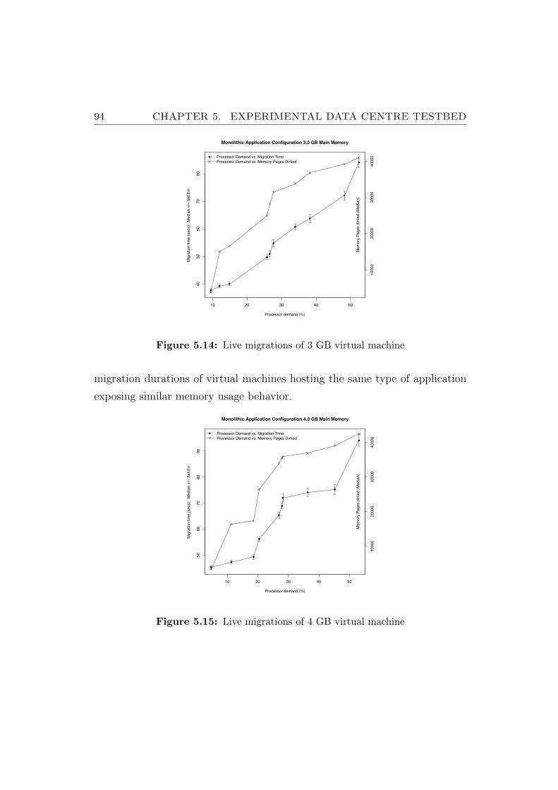
94 CHAPTER 5. EXPERIMENTAL DATA CENTRE TESTBED
!
!!
!
!
!
!
!
!
!
10 20 30 40 50
40
50
60
70
80
Processor demand (%)
Mig
ratio
n t
ime
(se
cs):
M
ed
ian
+/!
Std
.Err
.
Monolithic Application Configuration 3.0 GB Main Memory
10
00
02
00
00
30
00
04
00
00
Me
mo
ry P
ag
es d
irtie
d (
Me
dia
n)
! Processor Demand vs. Migration Time
Processor Demand vs. Memory Pages Dirtied
Figure 5.14: Live migrations of 3 GB virtual machine
migration durations of virtual machines hosting the same type of application
exposing similar memory usage behavior.
!
!
!
!
!
!
!
!
!
!
10 20 30 40 50
50
60
70
80
90
Processor demand (%)
Mig
ratio
n t
ime
(se
cs):
M
ed
ian
+/!
Std
.Err
.
Monolithic Application Configuration 4.0 GB Main Memory
10
00
02
00
00
30
00
04
00
00
Me
mo
ry P
ag
es d
irtie
d (
Me
dia
n)
! Processor Demand vs. Migration Time
Processor Demand vs. Memory Pages Dirtied
Figure 5.15: Live migrations of 4 GB virtual machine
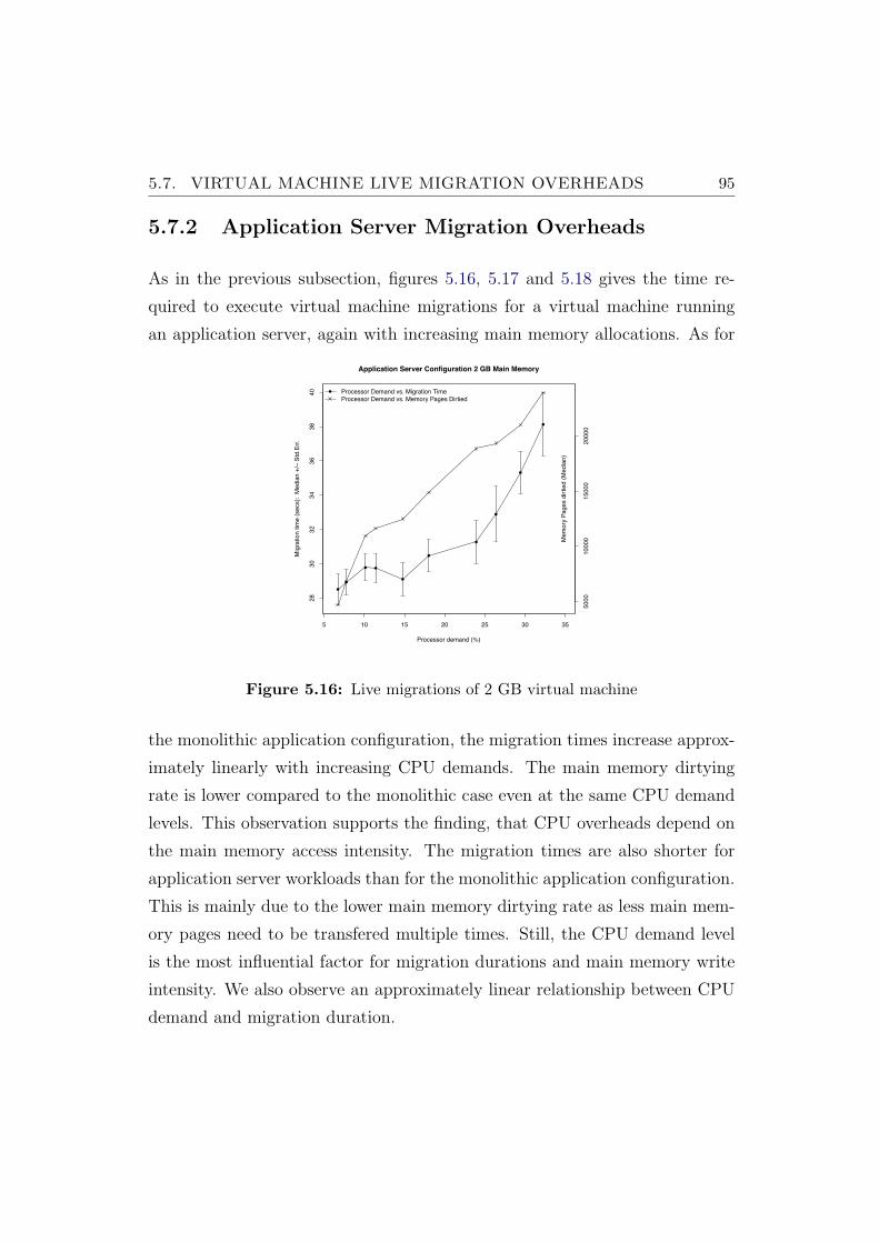
5.7. VIRTUAL MACHINE LIVE MIGRATION OVERHEADS 95
5.7.2 Application Server Migration Overheads
As in the previous subsection, figures 5.16, 5.17 and 5.18 gives the time re-
quired to execute virtual machine migrations for a virtual machine running
an application server, again with increasing main memory allocations. As for
!
!
! !
!
!
!
!
!
!
5 10 15 20 25 30 35
28
30
32
34
36
38
40
Processor demand (%)
Mig
ratio
n t
ime
(se
cs):
M
ed
ian
+/!
Std
.Err
.
Application Server Configuration 2 GB Main Memory
50
00
10
00
01
50
00
20
00
0
Me
mo
ry P
ag
es d
irtie
d (
Me
dia
n)
! Processor Demand vs. Migration Time
Processor Demand vs. Memory Pages Dirtied
Figure 5.16: Live migrations of 2 GB virtual machine
the monolithic application configuration, the migration times increase approx-
imately linearly with increasing CPU demands. The main memory dirtying
rate is lower compared to the monolithic case even at the same CPU demand
levels. This observation supports the finding, that CPU overheads depend on
the main memory access intensity. The migration times are also shorter for
application server workloads than for the monolithic application configuration.
This is mainly due to the lower main memory dirtying rate as less main mem-
ory pages need to be transfered multiple times. Still, the CPU demand level
is the most influential factor for migration durations and main memory write
intensity. We also observe an approximately linear relationship between CPU
demand and migration duration.
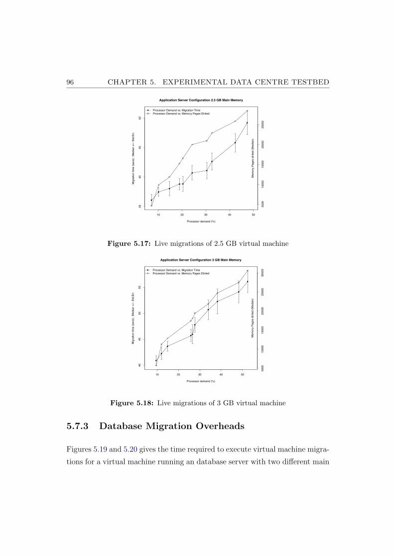
96 CHAPTER 5. EXPERIMENTAL DATA CENTRE TESTBED
!
!
!
! !
!
!
!
!
!
10 20 30 40 50
35
40
45
50
Processor demand (%)
Mig
ratio
n t
ime
(se
cs):
M
ed
ian
+/!
Std
.Err
.
Application Server Configuration 2.5 GB Main Memory
50
00
10
00
01
50
00
20
00
02
50
00
Me
mo
ry P
ag
es d
irtie
d (
Me
dia
n)
! Processor Demand vs. Migration Time
Processor Demand vs. Memory Pages Dirtied
Figure 5.17: Live migrations of 2.5 GB virtual machine
!
!
!
!!
!
!
!
!
!
10 20 30 40 50
40
45
50
55
Processor demand (%)
Mig
ratio
n t
ime
(se
cs):
M
ed
ian
+/!
Std
.Err
.
Application Server Configuration 3 GB Main Memory5
00
01
00
00
15
00
02
00
00
25
00
03
00
00
Me
mo
ry P
ag
es d
irtie
d (
Me
dia
n)
! Processor Demand vs. Migration Time
Processor Demand vs. Memory Pages Dirtied
Figure 5.18: Live migrations of 3 GB virtual machine
5.7.3 Database Migration Overheads
Figures 5.19 and 5.20 gives the time required to execute virtual machine migra-
tions for a virtual machine running an database server with two different main
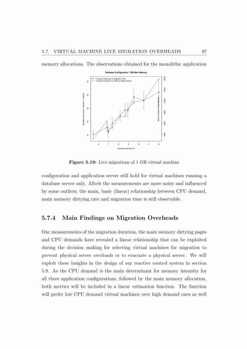
5.7. VIRTUAL MACHINE LIVE MIGRATION OVERHEADS 97
memory allocations. The observations obtained for the monolithic application
!
!
!
!
!
! !
!
!
!
6 7 8 9 10 11 12
16
18
20
22
24
Processor demand (%)
Mig
ratio
n t
ime
(se
cs):
M
ed
ian
+/!
Std
.Err
.
Database Configuration 1 GB Main Memory
40
00
60
00
80
00
10
00
01
20
00
14
00
0
Me
mo
ry P
ag
es d
irtie
d (
Me
dia
n)
! Processor Demand vs. Migration Time
Processor Demand vs. Memory Pages Dirtied
Figure 5.19: Live migrations of 1 GB virtual machine
configuration and application server still hold for virtual machines running a
database server only. Albeit the measurements are more noisy and influenced
by some outliers, the main, basic (linear) relationship between CPU demand,
main memory dirtying rate and migration time is still observable.
5.7.4 Main Findings on Migration Overheads
Our measurements of the migration duration, the main memory dirtying pages
and CPU demands have revealed a linear relationship that can be exploited
during the decision making for selecting virtual machines for migration to
prevent physical server overloads or to evacuate a physical server. We will
exploit these insights in the design of our reactive control system in section
5.9. As the CPU demand is the main determinant for memory intensity for
all three application configurations, followed by the main memory allocation,
both metrics will be included in a linear estimation function. The function
will prefer low CPU demand virtual machines over high demand ones as well
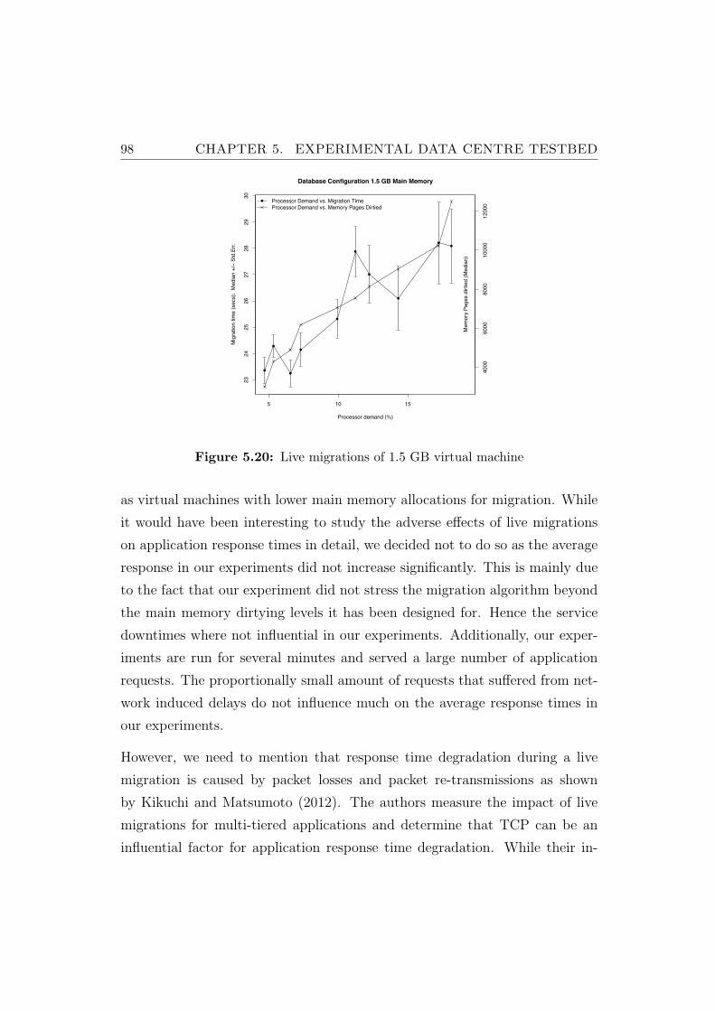
98 CHAPTER 5. EXPERIMENTAL DATA CENTRE TESTBED
!
!
!
!
!
!
!
!
!!
5 10 15
23
24
25
26
27
28
29
30
Processor demand (%)
Mig
ratio
n t
ime
(se
cs):
M
ed
ian +
/! S
td.E
rr.
Database Configuration 1.5 GB Main Memory
400
060
00
80
00
10
00
01
20
00
Me
mo
ry P
ag
es d
irtie
d (
Med
ian)
! Processor Demand vs. Migration Time
Processor Demand vs. Memory Pages Dirtied
Figure 5.20: Live migrations of 1.5 GB virtual machine
as virtual machines with lower main memory allocations for migration. While
it would have been interesting to study the adverse effects of live migrations
on application response times in detail, we decided not to do so as the average
response in our experiments did not increase significantly. This is mainly due
to the fact that our experiment did not stress the migration algorithm beyond
the main memory dirtying levels it has been designed for. Hence the service
downtimes where not influential in our experiments. Additionally, our exper-
iments are run for several minutes and served a large number of application
requests. The proportionally small amount of requests that suffered from net-
work induced delays do not influence much on the average response times in
our experiments.
However, we need to mention that response time degradation during a live
migration is caused by packet losses and packet re-transmissions as shown
by Kikuchi and Matsumoto (2012). The authors measure the impact of live
migrations for multi-tiered applications and determine that TCP can be an
influential factor for application response time degradation. While their in-
5.8. CONSOLIDATION OVERHEADS 99
vestigation is valid, their investigation is concerned with maximum response
times caused by service downtimes during a live migration. In contrast, we
focus on the migration process and show that not only the downtime, evoked
by the required ARP request, is a factor when studying migration overheads
in our experimental testbed.
5.8 Consolidation Overheads
The overheads for virtual machine live migrations influence on the design of dy-
namic workload management systems. Particularly static consolidation meth-
ods need to deal with the no-additive resource demands when co-locating vir-
tual machines on a single physical server. Each chart in this section has been
derived from five experiments lasting 30 minutes each. The median of each
measurement is taken and the median of the medians together with the stan-
dard deviation of the sample is depicted. All experiments are executed using
the hyper-thread setup which allows the assignment of one or two virtual cores
to a virtual machine. The main aim of this section is to introduce a consol-
idation overhead estimation function based on the CPU demands of a single
virtual machine hosting a given type of application. We will demonstrate that
overheads are dependent on the amount of virtual machines, the workload level
and type of virtual machine workload. While the interdependence of the three
factors is complex and can only be estimated accurately if the set of virtual
machines and their types is known in advance, we aim for a simple estimation
procedure that does not complicate the basic consolidation problem and can
be applied in a real world setting.
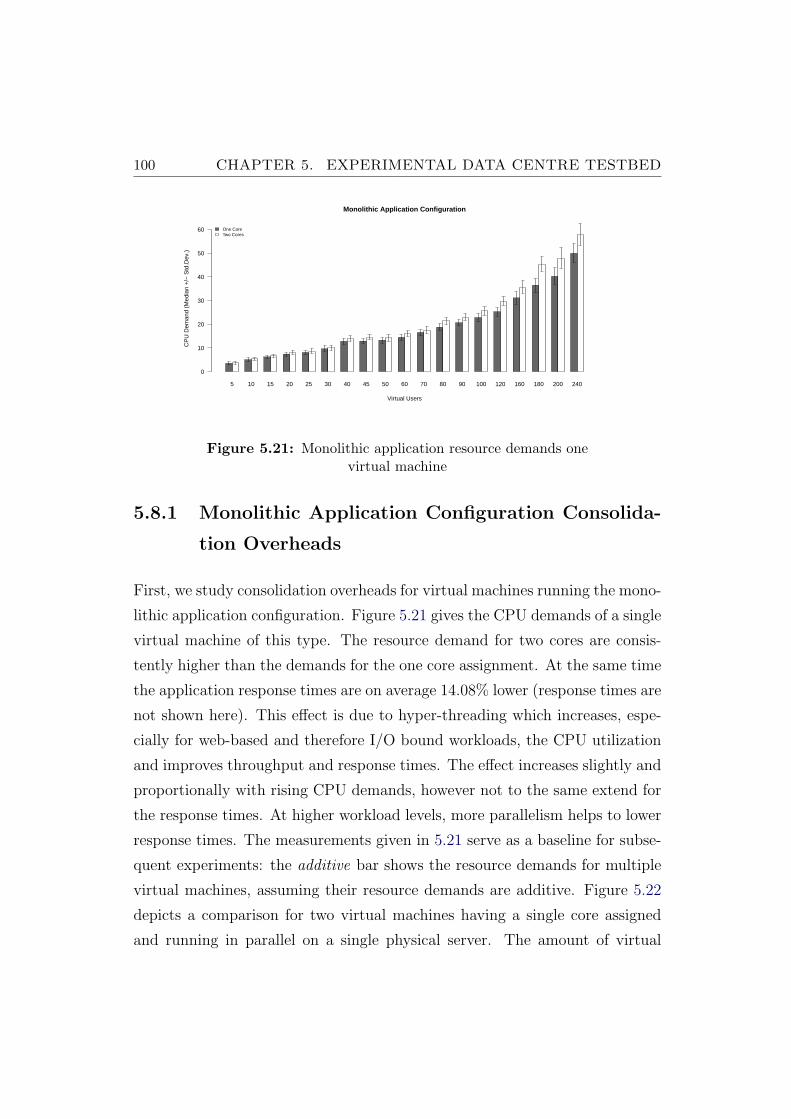
100 CHAPTER 5. EXPERIMENTAL DATA CENTRE TESTBED
5 10 15 20 25 30 40 45 50 60 70 80 90 100 120 160 180 200 240
Monolithic Application Configuration
Virtual Users
CP
U D
eman
d (M
edia
n +
/− S
td.D
ev.)
0
10
20
30
40
50
60 One CoreTwo Cores
Figure 5.21: Monolithic application resource demands onevirtual machine
5.8.1 Monolithic Application Configuration Consolida-
tion Overheads
First, we study consolidation overheads for virtual machines running the mono-
lithic application configuration. Figure 5.21 gives the CPU demands of a single
virtual machine of this type. The resource demand for two cores are consis-
tently higher than the demands for the one core assignment. At the same time
the application response times are on average 14.08% lower (response times are
not shown here). This effect is due to hyper-threading which increases, espe-
cially for web-based and therefore I/O bound workloads, the CPU utilization
and improves throughput and response times. The effect increases slightly and
proportionally with rising CPU demands, however not to the same extend for
the response times. At higher workload levels, more parallelism helps to lower
response times. The measurements given in 5.21 serve as a baseline for subse-
quent experiments: the additive bar shows the resource demands for multiple
virtual machines, assuming their resource demands are additive. Figure 5.22
depicts a comparison for two virtual machines having a single core assigned
and running in parallel on a single physical server. The amount of virtual
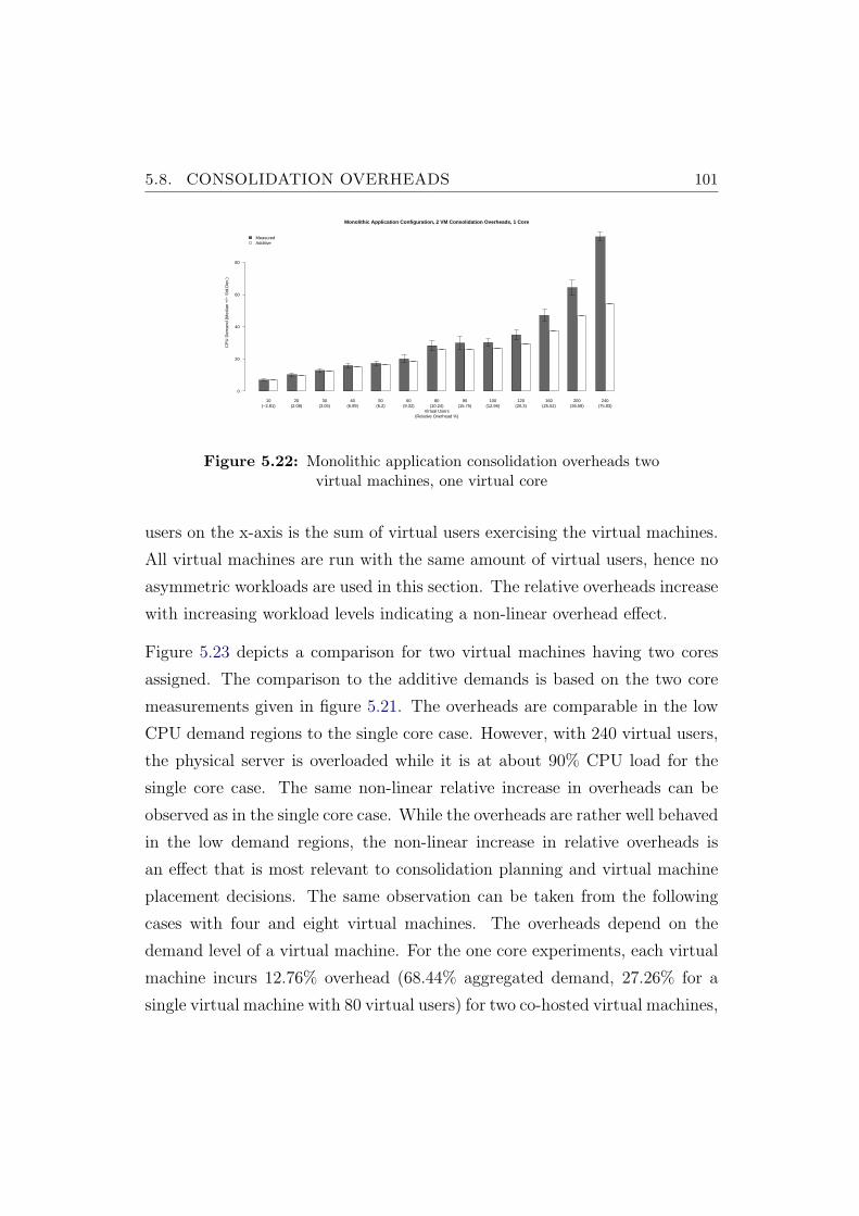
5.8. CONSOLIDATION OVERHEADS 101
10 20 30 40 50 60 80 90 100 120 160 200 240
Monolithic Application Configuration, 2 VM Consolidation Overheads, 1 Core
(Relative Overhead %)Virtual Users
CP
U D
eman
d (M
edia
n +
/− S
td.D
ev.)
0
20
40
60
80
MeasuredAdditive
(−2.81) (2.08) (3.05) (6.99) (6.2) (9.32) (10.24) (15.75) (12.96) (20.3) (25.52) (36.58) (75.83)
Figure 5.22: Monolithic application consolidation overheads twovirtual machines, one virtual core
users on the x-axis is the sum of virtual users exercising the virtual machines.
All virtual machines are run with the same amount of virtual users, hence no
asymmetric workloads are used in this section. The relative overheads increase
with increasing workload levels indicating a non-linear overhead effect.
Figure 5.23 depicts a comparison for two virtual machines having two cores
assigned. The comparison to the additive demands is based on the two core
measurements given in figure 5.21. The overheads are comparable in the low
CPU demand regions to the single core case. However, with 240 virtual users,
the physical server is overloaded while it is at about 90% CPU load for the
single core case. The same non-linear relative increase in overheads can be
observed as in the single core case. While the overheads are rather well behaved
in the low demand regions, the non-linear increase in relative overheads is
an effect that is most relevant to consolidation planning and virtual machine
placement decisions. The same observation can be taken from the following
cases with four and eight virtual machines. The overheads depend on the
demand level of a virtual machine. For the one core experiments, each virtual
machine incurs 12.76% overhead (68.44% aggregated demand, 27.26% for a
single virtual machine with 80 virtual users) for two co-hosted virtual machines,
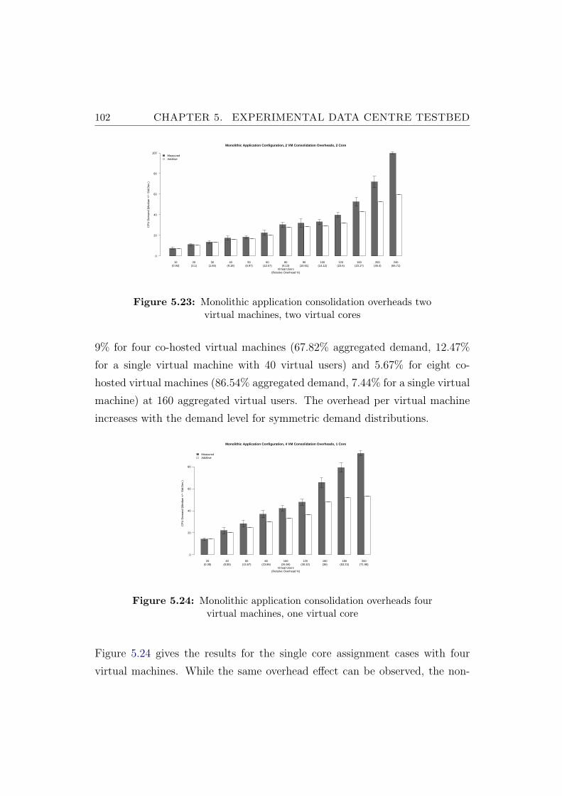
102 CHAPTER 5. EXPERIMENTAL DATA CENTRE TESTBED
10 20 30 40 50 60 80 90 100 120 160 200 240
Monolithic Application Configuration, 2 VM Consolidation Overheads, 2 Core
(Relative Overhead %)Virtual Users
CP
U D
eman
d (M
edia
n +
/− S
td.D
ev.)
0
20
40
60
80
100MeasuredAdditive
(0.94) (3.1) (1.65) (9.18) (6.97) (12.57) (8.13) (10.61) (14.12) (23.6) (23.17) (36.4) (66.71)
Figure 5.23: Monolithic application consolidation overheads twovirtual machines, two virtual cores
9% for four co-hosted virtual machines (67.82% aggregated demand, 12.47%
for a single virtual machine with 40 virtual users) and 5.67% for eight co-
hosted virtual machines (86.54% aggregated demand, 7.44% for a single virtual
machine) at 160 aggregated virtual users. The overhead per virtual machine
increases with the demand level for symmetric demand distributions.
20 40 60 80 100 120 160 180 200
Monolithic Application Configuration, 4 VM Consolidation Overheads, 1 Core
(Relative Overhead %)Virtual Users
CP
U D
eman
d (M
edia
n +
/− S
td.D
ev.)
0
20
40
60
80
MeasuredAdditive
(0.35) (8.55) (13.67) (23.86) (26.94) (30.32) (36) (53.23) (71.98)
Figure 5.24: Monolithic application consolidation overheads fourvirtual machines, one virtual core
Figure 5.24 gives the results for the single core assignment cases with four
virtual machines. While the same overhead effect can be observed, the non-
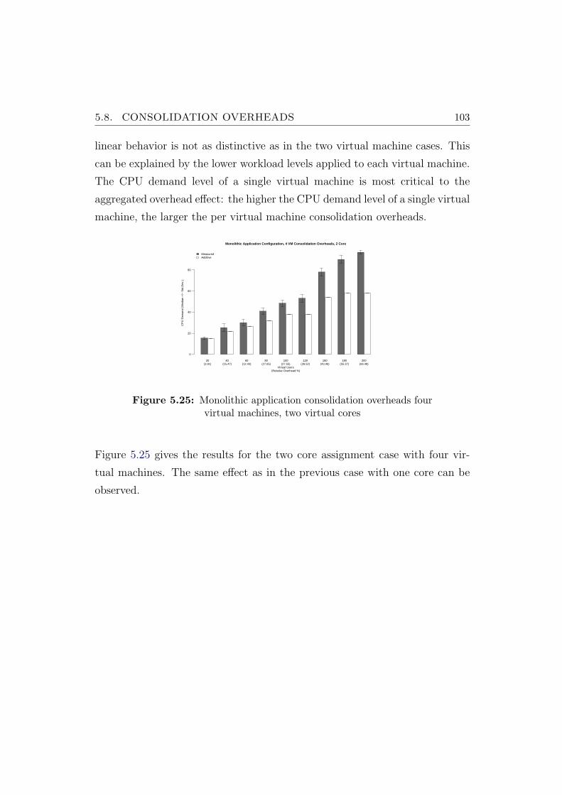
5.8. CONSOLIDATION OVERHEADS 103
linear behavior is not as distinctive as in the two virtual machine cases. This
can be explained by the lower workload levels applied to each virtual machine.
The CPU demand level of a single virtual machine is most critical to the
aggregated overhead effect: the higher the CPU demand level of a single virtual
machine, the larger the per virtual machine consolidation overheads.
20 40 60 80 100 120 160 180 200
Monolithic Application Configuration, 4 VM Consolidation Overheads, 2 Core
(Relative Overhead %)Virtual Users
CP
U D
eman
d (M
edia
n +
/− S
td.D
ev.)
0
20
40
60
80
MeasuredAdditive
(3.91) (15.47) (12.43) (27.65) (27.55) (39.52) (43.46) (55.37) (66.48)
Figure 5.25: Monolithic application consolidation overheads fourvirtual machines, two virtual cores
Figure 5.25 gives the results for the two core assignment case with four vir-
tual machines. The same effect as in the previous case with one core can be
observed.
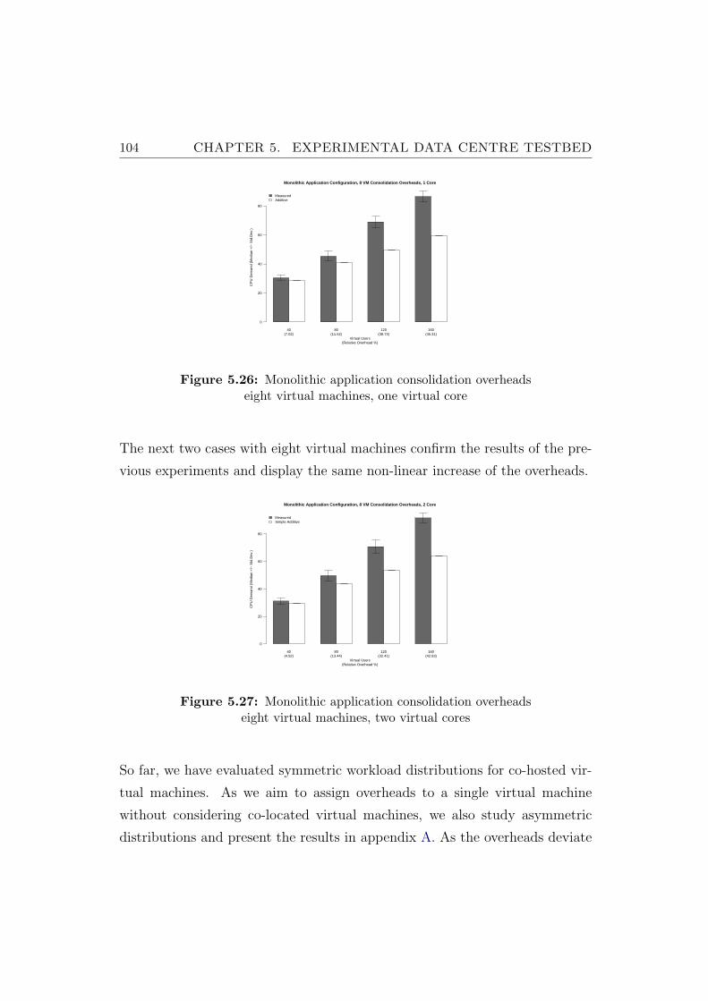
104 CHAPTER 5. EXPERIMENTAL DATA CENTRE TESTBED
40 80 120 160
Monolithic Application Configuration, 8 VM Consolidation Overheads, 1 Core
(Relative Overhead %)Virtual Users
CP
U D
eman
d (M
edia
n +
/− S
td.D
ev.)
0
20
40
60
80
MeasuredAdditive
(7.02) (11.52) (38.73) (45.31)
Figure 5.26: Monolithic application consolidation overheadseight virtual machines, one virtual core
The next two cases with eight virtual machines confirm the results of the pre-
vious experiments and display the same non-linear increase of the overheads.
40 80 120 160
Monolithic Application Configuration, 8 VM Consolidation Overheads, 2 Core
(Relative Overhead %)Virtual Users
CP
U D
eman
d (M
edia
n +
/− S
td.D
ev.)
0
20
40
60
80
MeasuredSimple Additive
(4.92) (13.44) (32.41) (42.93)
Figure 5.27: Monolithic application consolidation overheadseight virtual machines, two virtual cores
So far, we have evaluated symmetric workload distributions for co-hosted vir-
tual machines. As we aim to assign overheads to a single virtual machine
without considering co-located virtual machines, we also study asymmetric
distributions and present the results in appendix A. As the overheads deviate
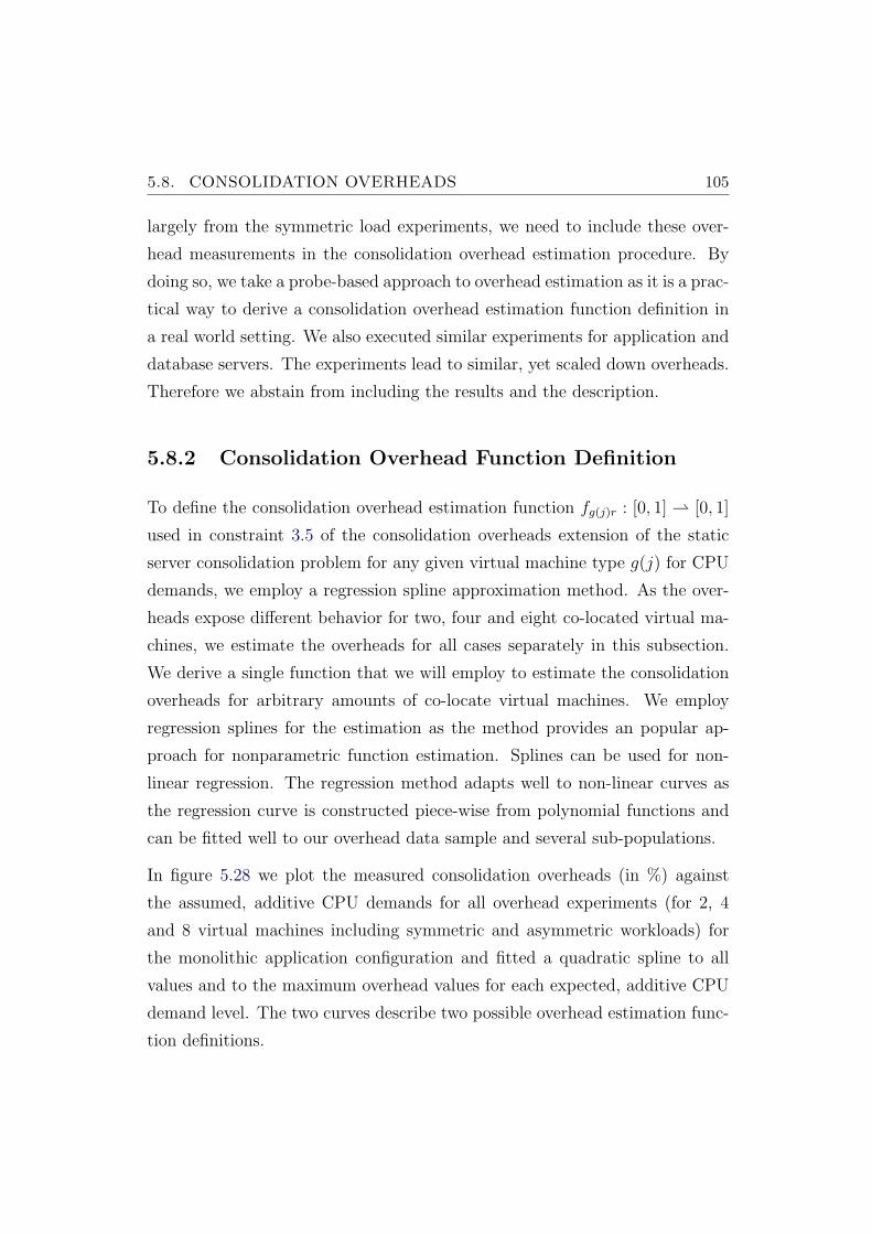
5.8. CONSOLIDATION OVERHEADS 105
largely from the symmetric load experiments, we need to include these over-
head measurements in the consolidation overhead estimation procedure. By
doing so, we take a probe-based approach to overhead estimation as it is a prac-
tical way to derive a consolidation overhead estimation function definition in
a real world setting. We also executed similar experiments for application and
database servers. The experiments lead to similar, yet scaled down overheads.
Therefore we abstain from including the results and the description.
5.8.2 Consolidation Overhead Function Definition
To define the consolidation overhead estimation function fg(j)r : [0, 1] ⇀ [0, 1]
used in constraint 3.5 of the consolidation overheads extension of the static
server consolidation problem for any given virtual machine type g(j) for CPU
demands, we employ a regression spline approximation method. As the over-
heads expose different behavior for two, four and eight co-located virtual ma-
chines, we estimate the overheads for all cases separately in this subsection.
We derive a single function that we will employ to estimate the consolidation
overheads for arbitrary amounts of co-locate virtual machines. We employ
regression splines for the estimation as the method provides an popular ap-
proach for nonparametric function estimation. Splines can be used for non-
linear regression. The regression method adapts well to non-linear curves as
the regression curve is constructed piece-wise from polynomial functions and
can be fitted well to our overhead data sample and several sub-populations.
In figure 5.28 we plot the measured consolidation overheads (in %) against
the assumed, additive CPU demands for all overhead experiments (for 2, 4
and 8 virtual machines including symmetric and asymmetric workloads) for
the monolithic application configuration and fitted a quadratic spline to all
values and to the maximum overhead values for each expected, additive CPU
demand level. The two curves describe two possible overhead estimation func-
tion definitions.
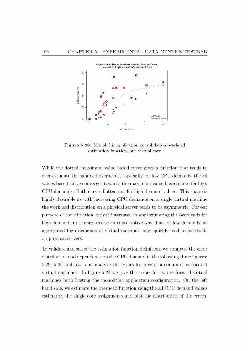
106 CHAPTER 5. EXPERIMENTAL DATA CENTRE TESTBED
● ●● ●
● ●
● ●
●
●
●
●
●
●
●
●
●
●
●
●
●
●
●
●
●
●
●
●
●
●
●
●
● ●
●
0 10 20 30 40
020
4060
80
Regression Spline Estimation Consolidation Overheads, Monolithic Application Configuration, 1 Core
CPU Demand (%)
CP
U O
verh
ead
(%)
●
●●
●
●
●●
●
●
●
● ●
●
●
●●
All ValuesMaximum Values
Figure 5.28: Monolithic application consolidation overheadestimation function, one virtual core
While the dotted, maximum value based curve gives a function that tends to
over-estimate the sampled overheads, especially for low CPU demands, the all
values based curve converges towards the maximum value based curve for high
CPU demands. Both curves flatten out for high demand values. This shape is
highly desirable as with increasing CPU demands on a single virtual machine
the workload distribution on a physical server tends to be asymmetric. For our
purpose of consolidation, we are interested in approximating the overheads for
high demands in a more precise an conservative way than for low demands, as
aggregated high demands of virtual machines may quickly lead to overloads
on physical servers.
To validate and select the estimation function definition, we compare the error
distribution and dependence on the CPU demand in the following three figures:
5.29, 5.30 and 5.31 and analyze the errors for several amounts of co-located
virtual machines. In figure 5.29 we give the errors for two co-located virtual
machines both hosting the monolithic application configuration. On the left
hand side, we estimate the overhead function using the all CPU demand values
estimator, the single core assignments and plot the distribution of the errors.
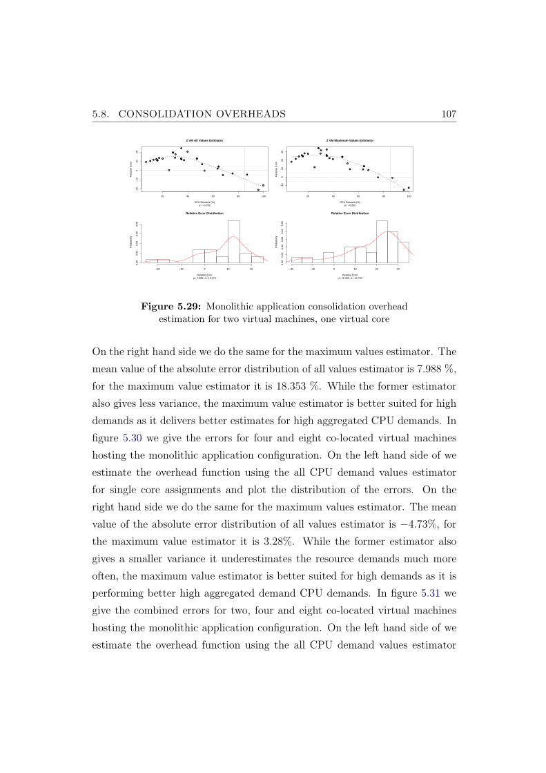
5.8. CONSOLIDATION OVERHEADS 107
●●
● ●
● ●
●
●
●
● ●
●
●
●●
●
●
●
●
●
●
●
●
●
●
●
●
●●
●
20 40 60 80 100
−20
−10
010
20
2 VM All Values Estimator
ρ= −0.769CPU Demand (%)
Rel
ativ
e E
rror ●
●
● ●
● ●
●
●
●
●●
●
●
●●
●
●●
●●
●
●
●
●
●●
●
● ●
●
20 40 60 80 100
−10
010
2030
2 VM Maximum Values Estimator
ρ= −0.835CPU Demand (%)
Rel
ativ
e E
rror
Relative Error Distribution
µ= 7.988, σ= 10.275Relative Error
Pro
babi
lity
−20 −10 0 10 20
0.00
0.02
0.04
0.06
0.08
Relative Error Distribution
µ= 18.353, σ= 12.792Relative Error
Pro
babi
lity
−20 −10 0 10 20 30
0.00
0.01
0.02
0.03
0.04
0.05
Figure 5.29: Monolithic application consolidation overheadestimation for two virtual machines, one virtual core
On the right hand side we do the same for the maximum values estimator. The
mean value of the absolute error distribution of all values estimator is 7.988 %,
for the maximum value estimator it is 18.353 %. While the former estimator
also gives less variance, the maximum value estimator is better suited for high
demands as it delivers better estimates for high aggregated CPU demands. In
figure 5.30 we give the errors for four and eight co-located virtual machines
hosting the monolithic application configuration. On the left hand side of we
estimate the overhead function using the all CPU demand values estimator
for single core assignments and plot the distribution of the errors. On the
right hand side we do the same for the maximum values estimator. The mean
value of the absolute error distribution of all values estimator is −4.73%, for
the maximum value estimator it is 3.28%. While the former estimator also
gives a smaller variance it underestimates the resource demands much more
often, the maximum value estimator is better suited for high demands as it is
performing better high aggregated demand CPU demands. In figure 5.31 we
give the combined errors for two, four and eight co-located virtual machines
hosting the monolithic application configuration. On the left hand side of we
estimate the overhead function using the all CPU demand values estimator
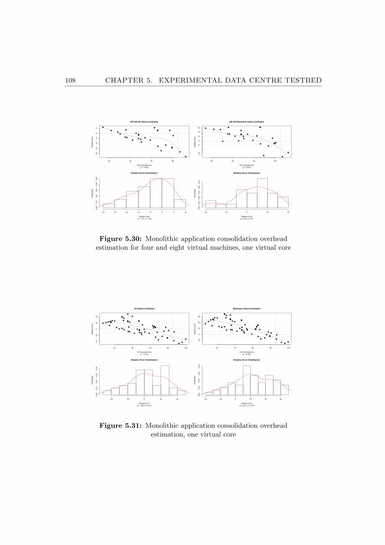
108 CHAPTER 5. EXPERIMENTAL DATA CENTRE TESTBED
●
●
●
●
●
●
●
●
●
●
●
●
●
●
●
●
●
●
●
●
●
●●
●●
●
●
●
20 40 60 80
−20
−15
−10
−5
05
4/8 VM All Values Estimator
ρ= −0.624CPU Demand (%)
Rel
ativ
e E
rror
●● ●
●
●
●
●
●
●
●
●
●
●
●
●
●
●
●
●
●
●
●●
●●
●
●
●
20 40 60 80
−15
−5
05
1015
4/8 VM Maximum Values Estimator
ρ= −0.674CPU Demand (%)
Rel
ativ
e E
rror
Relative Error Distribution
µ= −4.73, σ= 7.66Relative Error
Pro
babi
lity
−25 −20 −15 −10 −5 0 5 10
0.00
0.01
0.02
0.03
0.04
0.05
Relative Error Distribution
µ= 3.28, σ= 9.37Relative Error
Pro
babi
lity
−20 −10 0 10 20
0.00
0.01
0.02
0.03
0.04
0.05
Figure 5.30: Monolithic application consolidation overheadestimation for four and eight virtual machines, one virtual core
●●
● ●
● ●
●
●
●
● ●
●
●
●●
●
●
●
●
●
●
●
●
●
●
●
●
●●
●
●
●●
●
●●
●
●
●
●
●
●
●
●
●
●
●
●
●
●
●
● ●
●●
●
●
●
20 40 60 80 100
−20
−10
010
20
All Values Estimator
ρ= −0.723CPU Demand (%)
Rel
ativ
e E
rror ●
●
● ●
● ●
●
●
●
●●
●
●
●●
●
●●
●●
●
●
●
●
●●
●
● ●
●
●● ●
●
●●
●
●
●
●
●
●
●
●
●
●
●
●
●
●
●
●
●
● ●
●●
●
20 40 60 80 100
−10
010
2030
Maximum Values Estimator
ρ= −0.794CPU Demand (%)
Rel
ativ
e E
rror
Relative Error Distribution
µ= 1.85, σ= 11.07Relative Error
Pro
babi
lity
−20 −10 0 10 20
0.00
0.01
0.02
0.03
0.04
Relative Error Distribution
µ= 11.87, σ= 12.61Relative Error
Pro
babi
lity
−20 −10 0 10 20 30
0.00
0.01
0.02
0.03
0.04
Figure 5.31: Monolithic application consolidation overheadestimation, one virtual core
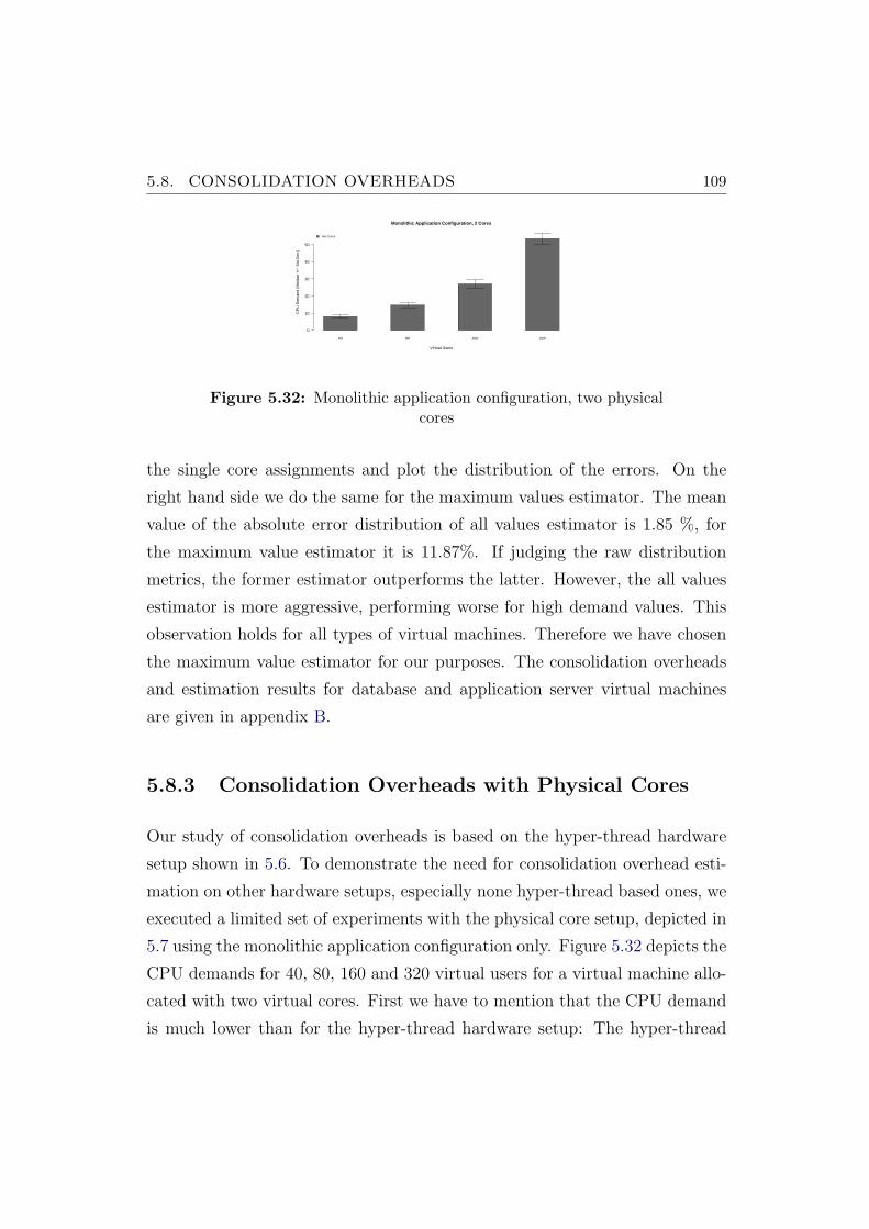
5.8. CONSOLIDATION OVERHEADS 109
40 80 160 320
Monolithic Application Configuration, 2 Cores
Virtual Users
CP
U D
eman
d (M
edia
n +
/− S
td.D
ev.)
0
10
20
30
40
50
Two Cores
Figure 5.32: Monolithic application configuration, two physicalcores
the single core assignments and plot the distribution of the errors. On the
right hand side we do the same for the maximum values estimator. The mean
value of the absolute error distribution of all values estimator is 1.85 %, for
the maximum value estimator it is 11.87%. If judging the raw distribution
metrics, the former estimator outperforms the latter. However, the all values
estimator is more aggressive, performing worse for high demand values. This
observation holds for all types of virtual machines. Therefore we have chosen
the maximum value estimator for our purposes. The consolidation overheads
and estimation results for database and application server virtual machines
are given in appendix B.
5.8.3 Consolidation Overheads with Physical Cores
Our study of consolidation overheads is based on the hyper-thread hardware
setup shown in 5.6. To demonstrate the need for consolidation overhead esti-
mation on other hardware setups, especially none hyper-thread based ones, we
executed a limited set of experiments with the physical core setup, depicted in
5.7 using the monolithic application configuration only. Figure 5.32 depicts the
CPU demands for 40, 80, 160 and 320 virtual users for a virtual machine allo-
cated with two virtual cores. First we have to mention that the CPU demand
is much lower than for the hyper-thread hardware setup: The hyper-thread
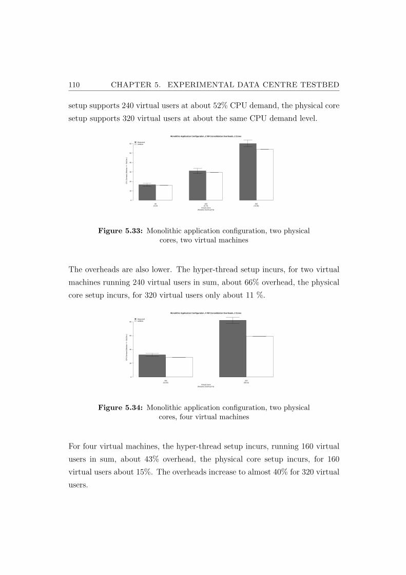
110 CHAPTER 5. EXPERIMENTAL DATA CENTRE TESTBED
setup supports 240 virtual users at about 52% CPU demand, the physical core
setup supports 320 virtual users at about the same CPU demand level.
80 160 320
Monolithic Application Configuration, 2 VM Consolidation Overheads, 2 Cores
(Relative Overhead %)Virtual Users
CP
U D
eman
d (M
edia
n +
/− S
td.D
ev.)
0
10
20
30
40
50
60MeasuredAdditive
(3.04) (5.73) (10.86)
Figure 5.33: Monolithic application configuration, two physicalcores, two virtual machines
The overheads are also lower. The hyper-thread setup incurs, for two virtual
machines running 240 virtual users in sum, about 66% overhead, the physical
core setup incurs, for 320 virtual users only about 11 %.
160 320
Monolithic Application Configuration, 4 VM Consolidation Overheads, 2 Cores
(Relative Overhead %)Virtual Users
CP
U D
eman
d (M
edia
n +
/− S
td.D
ev.)
0
20
40
60
80
MeasuredAdditive
(14.63) (39.54)
Figure 5.34: Monolithic application configuration, two physicalcores, four virtual machines
For four virtual machines, the hyper-thread setup incurs, running 160 virtual
users in sum, about 43% overhead, the physical core setup incurs, for 160
virtual users about 15%. The overheads increase to almost 40% for 320 virtual
users.
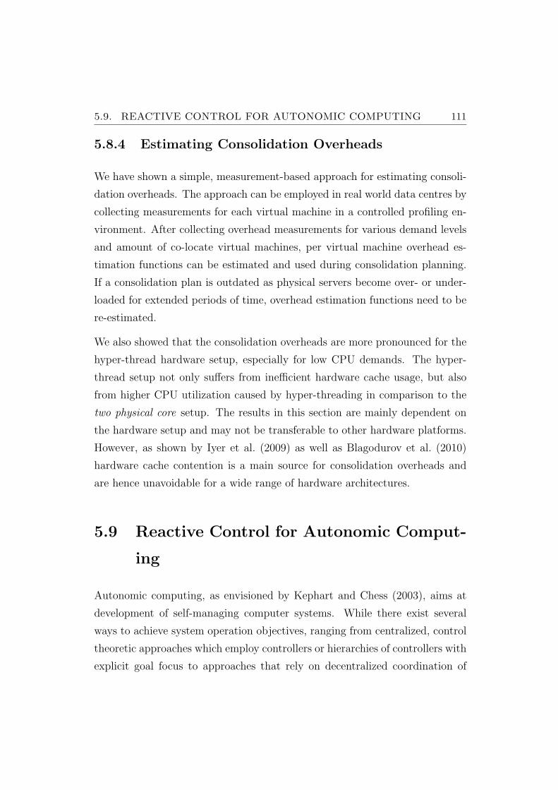
5.9. REACTIVE CONTROL FOR AUTONOMIC COMPUTING 111
5.8.4 Estimating Consolidation Overheads
We have shown a simple, measurement-based approach for estimating consoli-
dation overheads. The approach can be employed in real world data centres by
collecting measurements for each virtual machine in a controlled profiling en-
vironment. After collecting overhead measurements for various demand levels
and amount of co-locate virtual machines, per virtual machine overhead es-
timation functions can be estimated and used during consolidation planning.
If a consolidation plan is outdated as physical servers become over- or under-
loaded for extended periods of time, overhead estimation functions need to be
re-estimated.
We also showed that the consolidation overheads are more pronounced for the
hyper-thread hardware setup, especially for low CPU demands. The hyper-
thread setup not only suffers from inefficient hardware cache usage, but also
from higher CPU utilization caused by hyper-threading in comparison to the
two physical core setup. The results in this section are mainly dependent on
the hardware setup and may not be transferable to other hardware platforms.
However, as shown by Iyer et al. (2009) as well as Blagodurov et al. (2010)
hardware cache contention is a main source for consolidation overheads and
are hence unavoidable for a wide range of hardware architectures.
5.9 Reactive Control for Autonomic Comput-
ing
Autonomic computing, as envisioned by Kephart and Chess (2003), aims at
development of self-managing computer systems. While there exist several
ways to achieve system operation objectives, ranging from centralized, control
theoretic approaches which employ controllers or hierarchies of controllers with
explicit goal focus to approaches that rely on decentralized coordination of
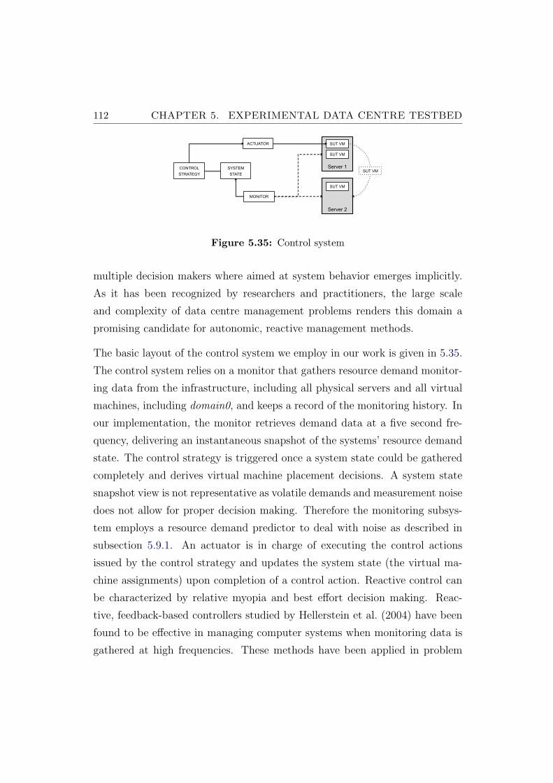
112 CHAPTER 5. EXPERIMENTAL DATA CENTRE TESTBED
!""#$%&$'()*+,)$
!!-,./01*,$0234562/)$4.$7,6.01,8$,9,1:$;$.,*/)8.$</1$633$4)<16.=10*=01,$,)22,.$
!!&>>,1$6)8$3/?,1$=+1,.+/38.$</1$1,./01*,$0234562/)$8,@),$>+:.4*63$.,19,1.$3/68$.=6=,.$
!!&)8,102345,8$
!!A/1763$
!!B9,13/68,8$
!!C/68$.=6=,$=16*D4)E$</1$941=063$76*+4),.$6)8$>+:.4*63$.,19,1.$=+1/0E+$,F>/),)263$
.7//=+4)E$?4=+$.3484)E$?4)8/?$/<$3,)E=+$GH$IJ$G$74)0=,K$
!"#$%"&'()*+%$(,-.$+/01$-2&34#&'-5-
GL$
CONTROL
STRATEGY
Server 1
SUT VM
SUT VM
MONITOR
ACTUATOR
SYSTEM
STATE
Server 2
SUT VM
SUT VM
Figure 5.35: Control system
multiple decision makers where aimed at system behavior emerges implicitly.
As it has been recognized by researchers and practitioners, the large scale
and complexity of data centre management problems renders this domain a
promising candidate for autonomic, reactive management methods.
The basic layout of the control system we employ in our work is given in 5.35.
The control system relies on a monitor that gathers resource demand monitor-
ing data from the infrastructure, including all physical servers and all virtual
machines, including domain0, and keeps a record of the monitoring history. In
our implementation, the monitor retrieves demand data at a five second fre-
quency, delivering an instantaneous snapshot of the systems’ resource demand
state. The control strategy is triggered once a system state could be gathered
completely and derives virtual machine placement decisions. A system state
snapshot view is not representative as volatile demands and measurement noise
does not allow for proper decision making. Therefore the monitoring subsys-
tem employs a resource demand predictor to deal with noise as described in
subsection 5.9.1. An actuator is in charge of executing the control actions
issued by the control strategy and updates the system state (the virtual ma-
chine assignments) upon completion of a control action. Reactive control can
be characterized by relative myopia and best effort decision making. Reac-
tive, feedback-based controllers studied by Hellerstein et al. (2004) have been
found to be effective in managing computer systems when monitoring data is
gathered at high frequencies. These methods have been applied in problem
5.9. REACTIVE CONTROL FOR AUTONOMIC COMPUTING 113
domains requiring real time behavior for control decision making and execu-
tion. Reactive control systems employ short term system state extrapolation
and prediction models. An obvious reason for this design decision is the gen-
eral uncertainty associated with the environments these systems operate in and
the limited availability of computational resources. Economical feasibility may
also constrain the use of computational demanding, potentially more accurate
methods for demand state prediction and assignment planning.
In order to provide system stability and to enable reliable, durable virtual ma-
chine placement decisions, the resource demands of virtual machines need to be
estimated in a way that ensures a representative estimate of the actual, highly
noised resource demand measurement data: estimates need to be as predictive
as possible,indicative for a trend and smooth. Decision algorithms used for real
time virtual machine placement typically make fast decisions on the basis of
the resource demands of the managed virtual machines. The workloads char-
acterizing most web-based enterprise applications makes it extremely difficult
to deduce a representative view of a resource demand from collected measures
that show large variability even at different time scales. Hence, any decision
based on instantaneous or average views of the resource demands may lead to
useless or even wrong virtual machine placement decisions.
In order to realize the potential gains in infrastructure efficiency, dynamic
resource allocation systems require robust and prudent runtime decisions for
deciding when a physical server should offload virtual machines and where the
offloaded machines should be placed. Since workload levels have been found to
change rapidly for enterprise applications as we have shown in chapter 4, but
has also been reported by Gmach et al. (2009), Cherkasova et al. (2009) and
Arlitt and Williamson (1997), control systems have to adapt to such variations
and provision resources over short time scales, usually on the order of minutes.
In order to reach decisions in a timely manner, control systems employ real time
decision making algorithms that scale for large problem instances as well. At
the same time, there is a need to take into account the cost of control, i.e., the
114 CHAPTER 5. EXPERIMENTAL DATA CENTRE TESTBED
switching costs associated with migrating virtual machines from one physical
server to another. Our measurements of the migration overheads in section 5.7
give an indication that excessive use of live migrations, that may occur in an
uncertain operating environment where resource demands are highly volatile,
may be harmful. As each migration decision is risky, control systems should
employ as much care as possible when deriving these decisions. Hence,real
time controllers should aim at system stability. The notion of stability is, ac-
cording to Nikolaou (2001), central in the study of dynamical systems. Infor-
mally speaking, stability is a systems property related to well-defined long-run
behavior. In our context, stability by itself may not necessarily guarantee sat-
isfactory performance, it is not conceivable that a control system may perform
well without delivering system stability if large, hard to estimate control action
overheads can be incurred that adversely affect application performance.
Intuitively, reactive control can be expected to require more control actions
than necessary, considering their myopic nature and the fact that limited
amounts of historic monitoring data do not provide much information about
the future resource demand behavior of virtual machines in volatile environ-
ments. Long term resource demand patterns are not taken into consideration
by reactive control and even though large control action overheads exist, agility
is the key feature that reactive methods are based upon. The determinants
that mostly influence on stability in our problem domain are
• resource demand estimation, prediction, overload and under-load detec-
tion,
• virtual machine migration candidate selection in response to under- or
overload detection and
• decisions concerning virtual machine reassignments.
As we will see in chapter 7, the three sub-problems and their interplay influ-
ence largely the stability of the virtual machine assignments and the control
5.9. REACTIVE CONTROL FOR AUTONOMIC COMPUTING 115
systems ability to meet the quality of service requirements for applications.
These sub-problems are particular to control chart based management meth-
ods. Threshold based event detection requires the definition of thresholds of
resource utilization on physical servers. A threshold violation (exceedance of
an upper threshold or shortfall of a lower threshold) potentially triggers an
immediate virtual machine migration. We use resource utilization thresholds
to define physical server demand states. A threshold is a tuple consisting of
an upper and lower utilization percentage. If the given state condition is met,
a server is said to be in a resource utilization state as defined by the respective
thresholds:
1. The under-loaded state is entered as the resource utilization is detected
to be below the lower threshold.
2. The normal state is entered as the resource utilization is detected to be
below the upper and above the lower threshold.
3. The over-loaded state is entered as the resource utilization is detected to
be above the upper threshold.
The problem of detecting substantial, non-transient overload or under-loads
on physical servers hosting virtual machines is crucial to the performance of
reactive control. Threshold based detection schemes are widely used to detect
deviations from normal, or average operations and have found acceptance in
industrial process control as well as performance management in computer
systems (Breitgand et al., 2011). The ability of a control system to detect and
to properly respond to these changes is critical to control system operations, as
predicting false-positive and false-negative alarms leads to unnecessary control
actions. While the detection and prediction are already non-trivial under real
time constraints, the proper definition of values for the thresholds is at least
as difficult as it heavily depends on the resource demand characteristics of the
hosted virtual machines.
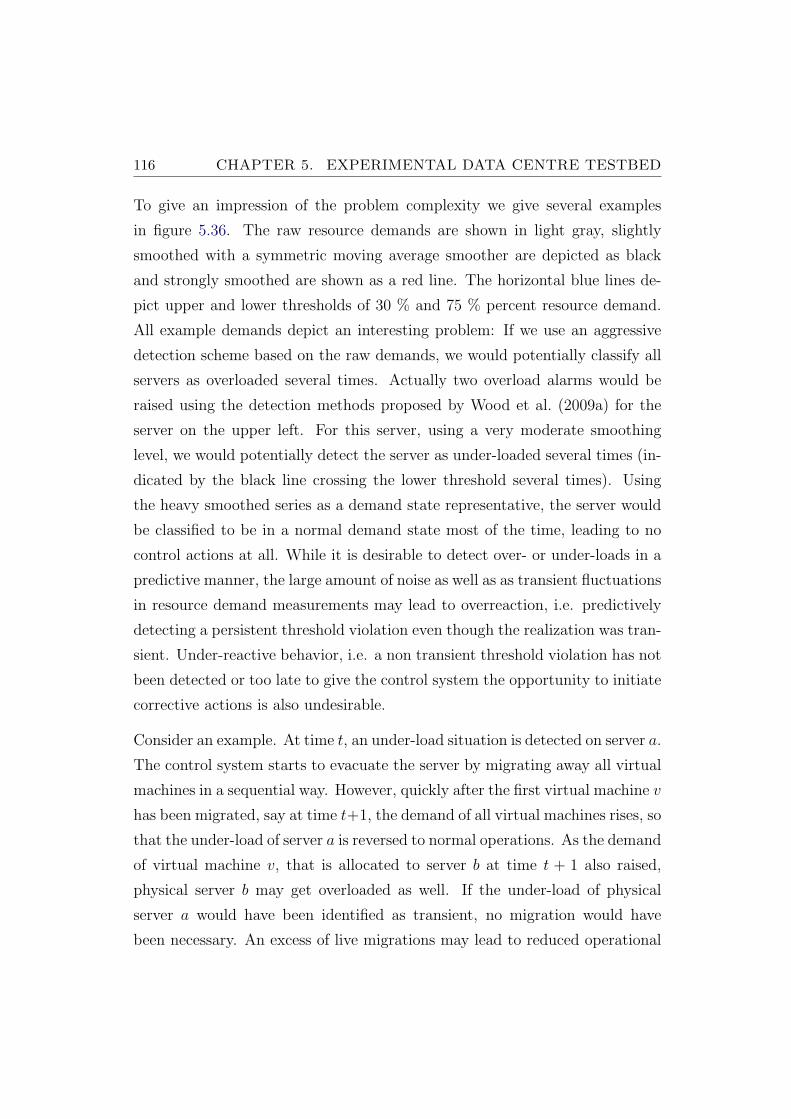
116 CHAPTER 5. EXPERIMENTAL DATA CENTRE TESTBED
To give an impression of the problem complexity we give several examples
in figure 5.36. The raw resource demands are shown in light gray, slightly
smoothed with a symmetric moving average smoother are depicted as black
and strongly smoothed are shown as a red line. The horizontal blue lines de-
pict upper and lower thresholds of 30 % and 75 % percent resource demand.
All example demands depict an interesting problem: If we use an aggressive
detection scheme based on the raw demands, we would potentially classify all
servers as overloaded several times. Actually two overload alarms would be
raised using the detection methods proposed by Wood et al. (2009a) for the
server on the upper left. For this server, using a very moderate smoothing
level, we would potentially detect the server as under-loaded several times (in-
dicated by the black line crossing the lower threshold several times). Using
the heavy smoothed series as a demand state representative, the server would
be classified to be in a normal demand state most of the time, leading to no
control actions at all. While it is desirable to detect over- or under-loads in a
predictive manner, the large amount of noise as well as as transient fluctuations
in resource demand measurements may lead to overreaction, i.e. predictively
detecting a persistent threshold violation even though the realization was tran-
sient. Under-reactive behavior, i.e. a non transient threshold violation has not
been detected or too late to give the control system the opportunity to initiate
corrective actions is also undesirable.
Consider an example. At time t, an under-load situation is detected on server a.
The control system starts to evacuate the server by migrating away all virtual
machines in a sequential way. However, quickly after the first virtual machine v
has been migrated, say at time t+1, the demand of all virtual machines rises, so
that the under-load of server a is reversed to normal operations. As the demand
of virtual machine v, that is allocated to server b at time t + 1 also raised,
physical server b may get overloaded as well. If the under-load of physical
server a would have been identified as transient, no migration would have
been necessary. An excess of live migrations may lead to reduced operational
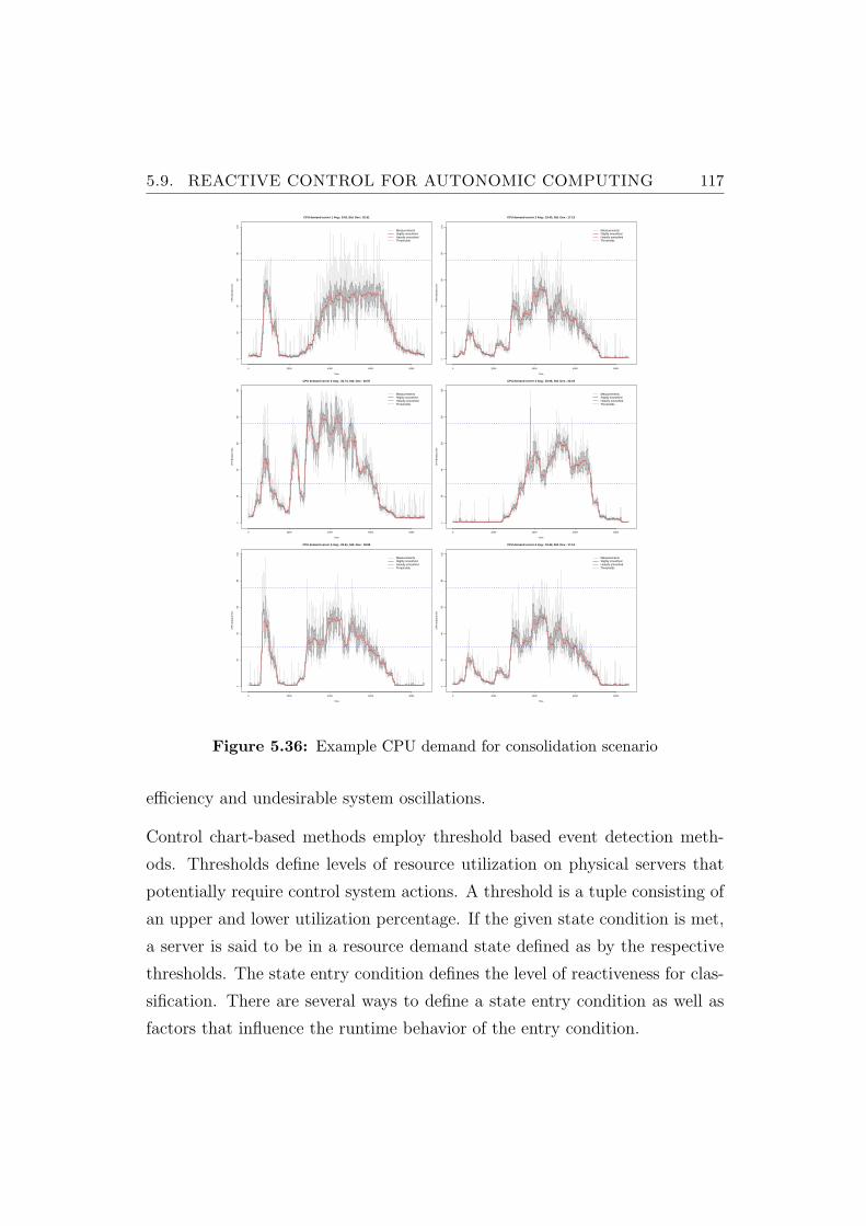
5.9. REACTIVE CONTROL FOR AUTONOMIC COMPUTING 117
CPU demand server 1 Avg.: 24.8, Std. Dev.: 20.51
Time
CP
U d
eman
d (%
)
0 2000 4000 6000 8000
020
4060
8010
0
MeasurementsSlighly smoothedHeavily smoothedThresholds
CPU demand server 2 Avg.: 19.43, Std. Dev.: 17.13
Time
CP
U d
eman
d (%
)
0 2000 4000 6000 8000
020
4060
8010
0
MeasurementsSlighly smoothedHeavily smoothedThresholds
CPU demand server 3 Avg.: 33.74, Std. Dev.: 26.97
Time
CP
U d
eman
d (%
)
0 2000 4000 6000 8000
020
4060
8010
0
MeasurementsSlighly smoothedHeavily smoothedThresholds
CPU demand server 4 Avg.: 20.96, Std. Dev.: 22.19
Time
CP
U d
eman
d (%
)
0 2000 4000 6000 8000
020
4060
8010
0
MeasurementsSlighly smoothedHeavily smoothedThresholds
CPU demand server 5 Avg.: 20.41, Std. Dev.: 18.89
Time
CP
U d
eman
d (%
)
0 2000 4000 6000 8000
020
4060
8010
0
MeasurementsSlighly smoothedHeavily smoothedThresholds
CPU demand server 6 Avg.: 19.43, Std. Dev.: 17.13
Time
CP
U d
eman
d (%
)
0 2000 4000 6000 8000
020
4060
8010
0
MeasurementsSlighly smoothedHeavily smoothedThresholds
Figure 5.36: Example CPU demand for consolidation scenario
efficiency and undesirable system oscillations.
Control chart-based methods employ threshold based event detection meth-
ods. Thresholds define levels of resource utilization on physical servers that
potentially require control system actions. A threshold is a tuple consisting of
an upper and lower utilization percentage. If the given state condition is met,
a server is said to be in a resource demand state defined as by the respective
thresholds. The state entry condition defines the level of reactiveness for clas-
sification. There are several ways to define a state entry condition as well as
factors that influence the runtime behavior of the entry condition.
118 CHAPTER 5. EXPERIMENTAL DATA CENTRE TESTBED
The results presented in the evaluation will show, that proper parameter tuning
is dependent on the overall workload characteristics and that it is possible to
tune parameters in a way that leads to sensible virtual machine placement
decisions.
As enterprise applications must meet performance-oriented quality of service
objectives an overload of a physical machine should be anticipated to allow
the control system to take remedial actions. It is thus necessary to derive
predictions for the estimated resource utilization. Such predictions allow an
automated data center control system to deal with anticipated resource uti-
lization in a proactive way by initiating migrations ahead of time, before a
resource shortage occurs.
The state entry condition defines the level of reactiveness for demand state
classification. In our work we employ a simple definition of an entry condition.
If the resource demand estimate is k-consecutive control cycles above or below
a threshold, the entry condition is met. If no entry condition is met, a server is
in the normal state. We refer to this entry condition definition as a sustained
decision that gives two desirable properties if the resource demand estimation
is appropriate (not over-reactive but accurate and representative):
1. The detection of transient demand state changes is reduced, reducing the
amount of triggered migrations.
2. Effective migration decisions can be derived as a non-transient overload
leads to a higher overload intensity, which in turn leads to a more effective
selection of migration candidates (overload is mitigated by migrating
virtual machines with higher demands).
There exist several ways to define a state entry condition. Both the state
entry condition and the demand estimation technique characteristics have to
be adjusted and tuned as we will discuss in chapter 7.
5.9. REACTIVE CONTROL FOR AUTONOMIC COMPUTING 119
The applied control loop algorithm is given in listing 1. The system state is
represented by the set I, the physical servers, J the set of virtual machines, the
set of historic control actions H and a function a : I ⇀ K ⊆ J), that returns
the set of all assigned virtual machines for a given physical server. The control
parameters are the triple P , where T is the set of upper and lower thresholds,
the demand predictor p, the detection delay d. We shortly describe the
necessary subroutines:
• filter-in-action: The subroutine filters out all physical servers that are
currently participating in a migration or have been participating a mi-
gration with the last minute. It uses the control action history H.
• state-classify : The subroutine assigns load states to all servers using the
demand predictor, threshold definitions and and detection delay param-
eters. It returns the disjunctive sets Io (over-loaded servers), In (normal
servers), Iu (under-loaded servers). The sets are ordered:
– Io is decreasingly ordered by the intensity of the overload, that is
the difference between the load state and the upper threshold for
CPU load. Higher overloaded servers should be evacuated first.
– In is decreasingly ordered by the sum of the normalized resource
demands for CPU and main memory.
– Iu is increasingly ordered by the sum of the normalized resource
demands for CPU and main memory.
• try-migrate: The subroutine tries to place a virtual machine on an under-
loaded or normally loaded server. According to the placement strategy,
it sorts the available target servers. Using the best-fit strategy, it first
sorts the normal load state servers in decreasing order according to the
sum of the normalized resource demands for CPU and main memory
and appends them to the set of under-loaded servers that are also sorted
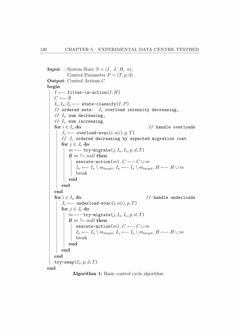
120 CHAPTER 5. EXPERIMENTAL DATA CENTRE TESTBED
Input : System State S = (I, J, H, a),Control Parameter P = (T, p, d)
Output: Control Actions Cbegin
I ←− filter-in-action(I,H)
C ←− ∅Io, In, Iu ←− state-classify(I, P)// ordered sets: Io overload intensity decreasing,
// In sum decreasing,
// Iu sum increasing
for i ∈ Io do // handle overloads
Je ←− overload-evac(i, a(i), p, T)// Je ordered decreasing by expected migration cost
for j ∈ Je dom←− try-migrate(j, In, Iu, p, d, T)if m != null then
execute-action(m), C ←− C ∪mIn ←− In \mtarget, Iu ←− Iu \mtarget, H ←− H ∪mbreak
end
end
endfor i ∈ Iu do // handle underloads
Je ←− underload-evac(i, a(i), p, T)for j ∈ Je do
m←− try-migrate(j, In, Iu, p, d, T)if m != null then
execute-action(m), C ←− C ∪mIn ←− In \mtarget, Iu ←− Iu \mtarget, H ←− H ∪mbreak
end
end
endtry-swap(In, p, d, T)
endAlgorithm 1: Basic control cycle algorithm
5.9. REACTIVE CONTROL FOR AUTONOMIC COMPUTING 121
in decreasing order. In contrast, using the worst-fit placement strategy,
it sorts the normal state servers in increasing order. It then identifies
the first server that can support the additional resource demands of the
virtual machine (the resource demands of the virtual machine have been
adopted by assigning the overheads of the domain0 proportionally to the
demands of the virtual machine) without exceeding the upper thresholds
for all resources. If no physical server can be found, no migration m is
proposed (and executed by the actuator), otherwise the selected server
is used as the target server mtarget for migration m.
• overload-evac: The subroutine first identifies all virtual machines, now
referred to as set O, that mitigate the overload on the physical server a
virtual machine is assigned to currently. A virtual machine qualifies for
this set if the server load state switches to normal (under the assumption
of additive CPU demands) if the virtual machine is moved from the
server. If no virtual machine qualified itself for O, O is set to a(i). O is
then sorted in increasing order according to the expected migration cost.
The cost is estimated using the following formula: (1+mcpu/100)×mram,
where mcpu is the current CPU load state of the virtual machine to be
migrated and mram the main memory allocation of the virtual machine.
In section 5.7 we have given a justification for the usage of the proposed
estimation procedure. In case of an overload, we want to migrate a virtual
machine that causes a minimum amount of overhead and mitigates the
overload sufficiently.
• underload-evac: The subroutine sorts the given virtual machines accord-
ing to the expected migration costs in decreasing order. In case of an
under-load, we first try to execute expensive migrations as we have suf-
ficient resources available to do so and second, if we can place virtual
machines with larger demands, we may be able to place virtual ma-
chines with less demands on the available servers without overloading
122 CHAPTER 5. EXPERIMENTAL DATA CENTRE TESTBED
them as we do not take consolidation overheads into consideration dur-
ing placement decisions. Lower demand virtual machines cause lower
consolidation overheads, as we have shown in section 5.8.
• try-swap: If an overload can not be mitigated because normal or under-
loaded servers can not be used for placing any virtual machine assigned
to the overloaded server, we try to exchange virtual machines on normal
or under-loaded servers in order to free capacity for the virtual machines
of the overloaded servers. A swap is executed in following way, similar
to how Wood et al. (2009a) proposed the implementation of swaps:
1. If a overloaded server exists, the assigned virtual machines are
sorted as done in overload-evac. Then, for each virtual machine
j ∈ Je possible target servers (non-overloaded ones) are selected
beginning with the highest loaded one.
2. We then check if it is possible to move a virtual machine from the
target server e to another, less loaded server (g) without violating
the upper thresholds. If it is possible, we then loop over all virtual
machines g ∈ Jg (sorted in increasing order of their normalized
resource demands for CPU and main memory) and check if we can
move a virtual machine to the server e without violating the upper
thresholds if j and g are moved to this server. If it is possible, we
issue the migration of g and j in a sequential order (by queuing up
the control actions, so they are executed in this order).
3. If no swaps are found to be feasible, no migrations are triggered.
We only enabled swaps for a very limited set of experiments, as swaps are a
not well known and evaluated way to increase operational efficiency.
Once an over- or under-load has been detected, the control system needs to
select virtual machines to migrate from a server to a target server. The deci-
sion which virtual machine to migrate depends on the resource demand states
5.9. REACTIVE CONTROL FOR AUTONOMIC COMPUTING 123
the other servers are in (a virtual machine might not have a potential receiver
under its current resource demands), the intensity of the current over-load and
the expected migration overheads. Generally speaking, a control system will
aim at taking effective, corrective actions afflicted at the lowest possible over-
heads. Wood et al. (2009a) introduces the concept of virtual machine swaps to
reduce wasted capacity and improved load balancing. A swap is an exchange
of two virtual machines hosted on different servers potential requiring a third
physical server to temporarily host a virtual machine, which then requires three
migrations to implement a swap instead of two in case of a directly executable
swap. Swaps may lead to even increased numbers of live migrations and select
high demand virtual machines which will lead to additional overheads. It is
not known whether swaps improve the efficiency of data centre operations and
do not contribute to system stability. We will show that swaps do not lead
to improvements, but lead to higher overheads and application performance
degradation.
Citrix Xen ships with a monitoring application that allows to monitor the
CPU, network and I/O demands of all virtual machines and physical servers.
On multi-core hardware, a virtual machine may be restricted to have access to
a limited amount of physical cores which can be controlled and configured in
a dynamic way. The CPU demand data for a virtual machine do not include
the CPU overhead caused in domain0 for processing I/O request on behalf
of other domains. As domain0 incurs non-neglibile CPU demand for I/O
intensive virtual machines, we account for the CPU demand by allotting to
virtual machines proportional to their current share of I/O demand on the
physical server. Similar to Wood et al. (2009a), each virtual machine is charged
a fraction of domain0 s CPU usage based on the proportion of the total I/O
requests made by that virtual machine.
As we employ a black-box approach that does not allow us to inspect a virtual
machine and to get memory demand measurements (the memory utilization is
only known to the guest operating system), it is not easy to collect memory
124 CHAPTER 5. EXPERIMENTAL DATA CENTRE TESTBED
demand measurements. While it is possible to observe memory accesses of vir-
tual machines through the use of shadow page tables, trapping each memory
access results in a signicant application slowdown as well as CPU overhead,w
e do not monitor main memory usage statistics. Thus, memory usage statis-
tics are not directly available and would have to be inferred from externally
observable swapping activity. Since substantial swapping activity is indicative
of memory shortage, this monitoring approach is not advisable, as swapping
significantly affects application performance. We assign memory in a static
way as it allows us to reason about CPU shortages.
5.9.1 Resource Demand Monitoring Architecture
Our reactive control system includes a monitoring subsystem for collecting
resource demands of virtual machines and physical servers that is depicted in
figure 5.37. For each physical server, the monitoring system runs a monitoring
thread that retrieves every five seconds resource demand measurements from
each physical server via HTTPS using the Citrix Xen monitoring API.
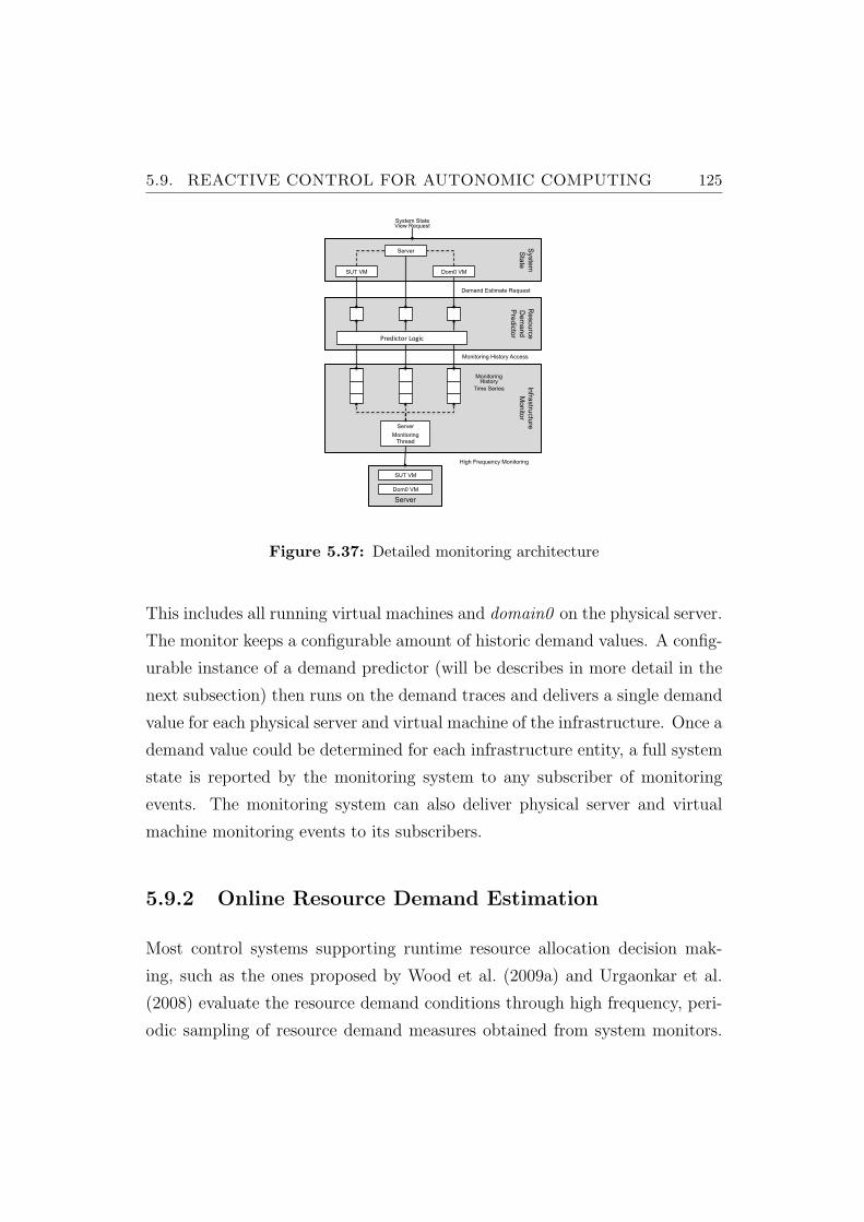
5.9. REACTIVE CONTROL FOR AUTONOMIC COMPUTING 125
!""#$%&$'()*+,)$ -.$
Infra
stru
ctu
re
Mo
nito
r
Server
Dom0 VM
SUT VM
Syste
m
Sta
te
Re
so
urc
e
De
ma
nd
Pre
dic
tor
Monitoring!!History
Time Series
/0,12*340$5462*$
High Frequency Monitoring
Server
Monitoring Thread
SUT VM Dom0 VM
Server
Demand Estimate Request
Monitoring History Access
System State View Request
Figure 5.37: Detailed monitoring architecture
This includes all running virtual machines and domain0 on the physical server.
The monitor keeps a configurable amount of historic demand values. A config-
urable instance of a demand predictor (will be describes in more detail in the
next subsection) then runs on the demand traces and delivers a single demand
value for each physical server and virtual machine of the infrastructure. Once a
demand value could be determined for each infrastructure entity, a full system
state is reported by the monitoring system to any subscriber of monitoring
events. The monitoring system can also deliver physical server and virtual
machine monitoring events to its subscribers.
5.9.2 Online Resource Demand Estimation
Most control systems supporting runtime resource allocation decision mak-
ing, such as the ones proposed by Wood et al. (2009a) and Urgaonkar et al.
(2008) evaluate the resource demand conditions through high frequency, peri-
odic sampling of resource demand measures obtained from system monitors.
126 CHAPTER 5. EXPERIMENTAL DATA CENTRE TESTBED
In the contexts of performance management of web server systems as pre-
sented by Abdelzaher et al. (2002) and Chen and Heidemann (2002), these
measurements are sufficient to make decisions about present and future work-
load behavior; that is to decide whether the demand condition on a physical
server is in an overloaded or stable state and whether it is necessary to trigger
control actions. On the other hand, these measurements are of little value for
the systems and workloads caused by modern enterprise applications that we
deal with. We can confirm that the resource measures obtained from resource
demand monitors are very volatile even at different time scales and tend to
become quickly obsolete as indicated by Dahlin (2000).
Figure 5.36 provides an example of the resource demands on a physical server
in one of our consolidation scenarios for all six physical servers. We display
the raw monitoring data as well as two smoothed versions. As we can see, the
smoothing factor determines the amount of threshold alarms, not smoothing
the monitoring data would lead to several false alarms. Consequently, the
selection of the resource demand estimation and prediction model for virtual
machines as well as the demand representation of a physical server directly
influences on the performance of a control strategy.
From our study of the main body of literature on resource demand estimation
and prediction in highly volatile environments, we conclude that the selec-
tion of an appropriate method depends on several factors and hence requires
a problem specific study. Albeit valuable contributions given by Andreolini
et al. (2008), Dinda and O’Hallaron (2000), Wolski (1998), Krishnamurthy
et al. (2003) exist, it is far from obvious which technique delivers good results
in our problem setting. Amongst the very few studies for predictive resource
allocation is the work of Xu et al. (2006). The work shows that CPU resource
allocation shares on a single physical server can be controlled in a proactive
way using autoregressive time series models to predict the resource demands
of virtual machines. It is however noted that the performance of a predictive
controller depends on the accuracy of the estimation and that the estimation
5.9. REACTIVE CONTROL FOR AUTONOMIC COMPUTING 127
values are often influenced by a high level of volatility. Based on an exten-
sive literature review, we identified several potential techniques for short term
prediction:
• Andreolini et al. (2008), Wolski (1998), Krishnamurthy et al. (2003) and
Cherkasova and Phaal (2002) propose simple smoothing techniques to
address the high level of noise and volatility in resource demand mea-
surements. Although smoothing does not directly relate to time series
forecasting, it can still be advantageous to smooth the raw measurement
stream in order to reduce out of scale values and to use the resulting se-
ries as a trend indicator as proposed by Lilja (2000). Wolski (1998) and
Krishnamurthy et al. (2003) use smoothing for forecasting purposes. One
of the advantages of smoothing methods is that they are lightweight and
can be implemented efficiently. We evaluate several smoothing methods
that have already been proposed by Andreolini et al. (2008) and Wolski
(1998) for resource demand state estimation and prediction. While the
performance of smoothing methods for one step ahead forecast based
on resource demand measurements has been evaluated in Wolski (1998),
their performance for k step ahead forecasts and trend extrapolation is
not well studied.
• More advanced, linear time series techniques have been studied by Dinda
and O’Hallaron (2000) and, to a limited extent by Andreolini et al.
(2008). The work of the former introduced autoregressive (AR), moving
average (MA), autoregressive moving average (ARMA), autoregressive
integrated moving average (ARIMA) and autoregressive fractional inte-
grated moving average (ARFIMA) models. Especially auto-regressive
models have been found to predict resource demands consistently to a
useful degree and to be compatible with runtime requirements in large
scale data centre control problems. However, according to Tran and Reed
(2004), Casolari and Colajanni (2009) and Baryshnikov et al. (2005), it
128 CHAPTER 5. EXPERIMENTAL DATA CENTRE TESTBED
is difficult or even impossible to retrieve an accurate prediction if the
auto-correlation of the measured data is low. Gmach et al. (2009) argues
that linear models are appropriate for short term prediction.
• The presented prediction models generate a single point forecast. How-
ever, the prediction quality is not constant, but varies depending on the
underlying series as well as the forecast horizon. Thus, a metric that
measures the estimated accuracy of the prediction is needed. Processes
that require forecast can then use the point forecast in combination with
the estimated accuracy to decide on further actions. As point estimates
for resource demands can only be expected to predict central tendencies
in face of large demand fluctuations, prediction methods for volatility are
usefully to amend point forecasts with a measurement of uncertainty. As
we have already seen in chapter 4, resource demands often exhibit time-
variation in the conditional volatility. Conditional heteroskedasticity in
time series has been studied in the literature on financial engineering and
econometrics, starting with the ARCH model of Engle (1982). Due to
time restrictions we do not present our results on volatility forecasts, as
we found that existing models are hard to select and to tune. We do not
use volatility forecasts in our control system design.
The fact that no method has found wide-spread acceptance or has been shown
to deliver good results on average in combination with the comments of Wood
et al. (2009a) on possible improvements reactive control may realize due to
optimal resource demand prediction, leads us to a detailed study of the pre-
diction and estimation problem. In particular, we will study the performance
of several methods and evaluate possible improvements.
In the following, we introduce the resource demand predictors that we use in
our study to obtain a representative view from high frequency resource demand
measurements. As indicated by Andreolini et al. (2008), a resource demand
5.9. REACTIVE CONTROL FOR AUTONOMIC COMPUTING 129
predictor should not simply filter and smooth noise but should deliver an esti-
mate of the actual resource demands that can be used subsequently by a control
system to detect over and under-load situations or to select virtual machines
that should be migrated. Hence we seek for the right compromise between
accuracy and responsiveness of a predictor. As predictors we will consider
simple moving average (SMA), exponential moving average (EMA), median
alpha trimmed mean (ATM), two sided quartile-weighted median(QWM) and
autoregressive (AR) time series models. The notation SMAn, will denote the
amount of historic measurements (window of length n) that the predictor is
applied to. For smoothing techniques, this is simply the window the smoother
is applied to, for time series models it is the time series that is used to fit a
model. We exclude several linear time series models from our study due to
their runtime requirements for model fitting as will be shown in section 6.3.
Simple Moving Average: The most basic one of the considered smooth-
ing filters is the simple moving average (SMA) technique. It computes the
unweighted mean of the last n resource measures. That is,
SMAn(~ajr) =1
n
n∑i=1
aijr (5.1)
As stated before, SMA is a very lightweight smoothing filter. But as all mea-
sures are weighted equally, the filter tends to introduce a delay with respect
to the raw time series. The delay increases with subject to the window size n.
Hence we may expect bad accuracy and reactiveness results for SMA.
Exponential Moving Average: In order to mitigate the delay effect in SMA
and in order to give more recent measures a higher relevance, Exponential
Moving Average (EMA) weights more recent measures higher than the older
130 CHAPTER 5. EXPERIMENTAL DATA CENTRE TESTBED
ones. These weights fall off exponentially, that is,
EMAn(~ajr) = α ∗ anjr + (1− α) ∗ EMAn−1(a1jr, a
2jr, . . . , a
n−1jr ) (5.2)
EMA1(~ajr) = a1jr (5.3)
with α = 2/(n+ 1).
Median: In some cases, the median smoothing filter can be useful, partic-
ularly if the measurement sequence contains randomly occurring asymmetric
outliers as stated by Wolski (1998). For the calculation of the median, the
measurements in the time series must be sorted by its value first. In the fol-
lowing, ~x denotes the time series ordered ascending by its values. That is,
~x = {ajr|aijr ≤ ai+1jr , 1 ≤ i < n}. Then the median filter is
Median(~x) =
~xn+12
if n is odd
12
(~xn
2+ ~xn
2+1
)if n is even
(5.4)
according to Haddad and Parsons (1991), the median filter rejects extreme
outliers, but tends to produce a considerable amount of jitter.
Alpha Trimmed Mean: One combination of mean based approach with the
class of median filters is the alpha trimmed mean (ATM). First, a window of
the central n − 2 ∗ α ∗ n values of ~ajr is taken. With k being the number of
values to be trimmed on each side, i.e. k = bα ∗ nc, and 0 < α < 0.5, the
definition of the ATM is
ATMn(~ajr) =1
n− 2r
n−r∑i=r+1
aijr (5.5)
Two Sided Quartile-Weighted Median: Another Median based approach
is the Two Sided Quartile-Weighted Median. It is considered to be a robust
statistic that is independent of any assumption on the distribution of the re-
5.9. REACTIVE CONTROL FOR AUTONOMIC COMPUTING 131
source measures Duffield and Lo Presti (2002). With Qp denoting the p %
percentile, the two sided quartile-weighted median is defined as
QWMn(~ajr) =Q.75(a1
jr, . . . , anjr) + 2 ∗Q.5(a1
jr, . . . , anjr) +Q.25(a1
jr, . . . , anjr)
4(5.6)
Autoregressive Time Series Model: The series ~ajr is an autoregressive
time series process of order p if
atjr = φ1a1jr + φ2a
2jr + · · ·+ φpa
pjr + wt (5.7)
where φ1, . . . , φp are the autoregressive coefficients of the model with φp 6= 0
for an order p process. The order p of the filter is generally very much less
than the length of the series. wt represents the noise term or residue and is
almost always assumed to be white noise. The AR(p) process shown in 5.7 can
be written in short as
atjr =
p∑i=1
φiaijr + wt (5.8)
~ajr is already known as it is the measured resource utilization. Thus, the main
task in AR is to find the best values for φ1, . . . , φp for a given time series
~ajr.There are two main categories for computing the AR coefficients: the least
squares and the Burg method. For both methods, several variants are known.
The most common least squares method, for example, is based upon the Yule-
Walker equations. By multiplying 5.8 by adjr, taking the expectation values
and normalizing, a set of linear equations can be derived Box et al. (2008).
These linear equations are called the Yule-Walker equations and can be solved
efficiently.

132 CHAPTER 5. EXPERIMENTAL DATA CENTRE TESTBED
Detection Delay 36, Worst Fit, 75/30 Thresholds
Realized Efficiency: 19.28 %, Expected: 23.61 %Time (5 Seconds Frequency)
Req
uire
d S
erve
rs
0 2000 4000 6000 8000
4.0
4.5
5.0
5.5
6.0
Required ServersExpected Servers
Detection Delay 1, Best Fit, 75/30 Thresholds
Realized Efficiency: 19.77 %, Expected: 23.61 %Time (5 Seconds Frequency)
Req
uire
d S
erve
rs
0 2000 4000 6000 80004.
04.
55.
05.
56.
0
Required ServersExpected Servers
Figure 5.38: Baseline examples
5.10 Expectation Baselines
For our study, we require a point of reference, comparable to lower or upper
bounds for optimization problems. We would like to know what performance a
reasonable reactive control system may deliver in terms of delivered operational
efficiency and the amount of virtual machine live migrations required for any
workload scenario. Without a reference, we would not know what performance
levels can be reasonably expected. As we pre-compute the workload scenarios
and are able to defer the resource demands for all virtual machines at any
point in time (figure 5.9 shows the service demand for a virtual machines), we
use the assignment transition problem with overheads presented in section 3.3
to compute the amount of expected efficiency and amount of migrations on
an hourly basis. Figure 5.38 gives an example for a pre-computed efficiency
baseline and the realized efficiency for two reactive control experiment runs.
The red, dashed line depicts the amount of physical servers required for each
hour time slot of the 24 hour period of the scenario’s consolidation problem.
The grey solid line depicts the amount of servers actually required by the
reactive controls system during one experiment run.
Chapter 6
Evaluation Demand Prediction
Forecasting is like driving a car blindfolded with help from some-
one looking out of the rear window.
by Brian G. Long, Ph.D.
Dynamic management of virtualized data centres requires methods to identify
and estimate current as well as future resource demands of virtual machines
and physical servers. In this chapter, we analyze prediction techniques for
CPU demands of physical servers and virtual machines. The dedication of a
whole chapter may seem excessive, however the behavior of a reactive control
depends crucially on the applied predictor. As the characteristics of resource
demands generated by web-based enterprise applications make it difficult to
deduce a representative view from collected measurements that exhibit large
volatility at different time scales, techniques are required that mitigate prob-
lems with instantaneous views that may lead to ineffective control actions.
Virtual machine placement decisions and consequently the stability of virtual
machine assignments critically depend on the performance and characteristics
of the employed estimation technique. We evaluate resource demand predictors
133
134 CHAPTER 6. EVALUATION DEMAND PREDICTION
in terms of quality (accuracy and predictive power, responsiveness, stability)
and feasibility (runtime requirements). Especially accuracy and responsive-
ness are in conflicting with stability, as an estimator should not deliver highly
volatile values. A predictor giving optimal results for the three properties may
not exist. Hence, an acceptable trade-off needs to determined for the partic-
ular domain of application. Therefore an evaluation of possible predictors is
mandatory when designing a reactive control system. According to Andreolini
et al. (2008), a control system that is to take immediate actions may prefer
a reactive predictor that delivers high accuracy, while a control system that
has to apply care when triggering control actions may prefer a less accurate
and less responsive predictor. We show that the exponential moving average
is a preferable predictor in our domain and that it is not very likely to find a
better predictor.
Our evaluation is based on two data sets: the resource demand data set studied
in chapter 4 and a data set that we generated using our data centre benchmark.
It consists of six runs of static consolidation, containing CPU demand traces
of 36 physical servers and altogether 56 virtual machine traces recorded at a
frequency of five seconds for a time period of twelve hours. We use the two data
sets, as the traces in the first expose pronounced patterns, while the second
data set does not.
6.1 Excluded Prediction Models
We evaluated several prediction models that we did not include in our study
as the models did not deliver promising results.
Smoothing based Auto-regressive Time Series Model: As indicated by
Andreolini et al. (2008), Casolari and Colajanni (2009) and Baryshnikov et al.
(2005), auto-regressive time series models unfold their strength especially for
time series with recurring patterns and high, significant auto-correlation values.
6.1. EXCLUDED PREDICTION MODELS 135
Noised measurements may lead worse prediction results as the auto-correlation
values are negatively influenced by random fluctuations and large levels of noise
(as we have depicted in figure 4.4 for our resource demand data set). If a series
exposes significant positive auto-correlation values for a given lag, a resource
measurements may be used to predict the demand value about that lag into the
future. However, according to Tran and Reed (2004), Casolari and Colajanni
(2009) and Baryshnikov et al. (2005), it is difficult or even impossible to retrieve
an accurate prediction if the auto-correlation of the measured data is low. A
way to improve the forecast accuracy of autoregressive models is to change the
prediction basis from the raw measurements to a smoothed equivalent, if the
smoothed series exposes higher auto-correlation values than the raw series. As
a smoothed series better describes the central tendencies of a series, we may
expect better forecast for the tendencies. We evaluated the smoothing based
autoregressive time series model, that uses an exponential moving average
with window size of twelve for the prediction of the raw series. Our results
did not indicate an improvement, neither for accuracy nor for reactiveness.
While the smoothed series improved auto-correlation values, the forecasts did
not improve, as the smoothed series introduced forecasting errors that were
not compensated by the improved performance of the forecasting model. An
ex-post smoothed series did introduce non-compensable lagging of the forecast.
Linear Regression Extrapolation: Baryshnikov et al. (2005) proposes a
simple model that uses linear regression to forecast the central tendency of a
series. While this model delivered results similar to the average performance of
the smoothing techniques for one step ahead forecasts, its accuracy decreased
substantially for 3, 6 and 12 steps ahead and did not deliver useful results for
24 and 36 steps.
Smoothing based Linear Extrapolation: Inspired by Baryshnikov et al.
(2005), Andreolini et al. (2008) propose an extrapolation approach based on
a smoothed series. Rather estimating the trend based on the raw series the
smoothed series is taken. However, the model suffered from the same problems
136 CHAPTER 6. EVALUATION DEMAND PREDICTION
as the linear regression extrapolation model.
6.2 Accuracy Measures
There exist several measures of forecast accuracy defined for the difference of
forecast to actual time series values. Hyndman and Koehler (2006) give an
exhaustive survey over such measures. For highly volatile time series, these
measurements do no reflect a predictor’s ability to predict central tendencies:
whether a time series is following an upward or downward trend or whether
it is stabilizing. As outliers are not predictable and large levels of non-normal
noise would distort standard accuracy measurements, we opt for a comparison
of the predicted values with the ex-post smoothed time series. That is a
time series derived using a symmetric moving average filter with an odd sized
smoothing window. In this way the same amount of past as well as future
values are included into he smoothing process that leads to a less noisy, yet
representative version of the raw series. In figure 6.1 we show an example of
the smoothed version as the black line, the grey line is the raw series, the red
line is the series given by an EMA12 predictor for one step ahead forecasts.
The error series in figure 6.1, first given for the raw series then for the ex-post
smoothed series reveals that the error statistics are influenced by short, one
value demand spikes that can not be predicted well. Therefore, as a reference
for judging on the quality of a predictor, we use the ex-post smoothed time
series atjr.
As no single best accuracy measurement exists, several authors such as Bow-
erman et al. (2004) and Box et al. (2008) recommend different measurement
metrics; we voted for scale-dependent measurements as these are useful when
different methods are compared on the same set of data. When data sets
with different scalings are being compared, then these measurements should
be avoided. The mean square error (MSE) is generally more sensitive to out-
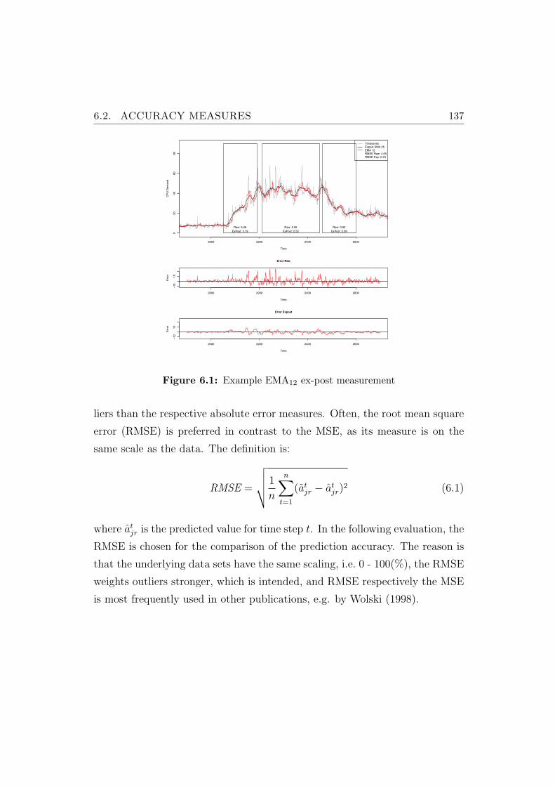
6.2. ACCURACY MEASURES 137Lookahead 1
Time
CP
U D
em
and
2000 2200 2400 2600
020
40
60
80
Timeseries
Expost SMA 25
EMA 12
RMSE Raw: 4.65
RMSE Exp: 2.24
Raw: 5.06
ExPost: 3.19
Raw: 5.95
ExPost: 2.52
Raw: 3.92
ExPost: 2.09
Error Raw
Time
Err
or
2000 2200 2400 2600
!10
10
Error Expost
Time
Err
or
2000 2200 2400 2600
!10
10
Figure 6.1: Example EMA12 ex-post measurement
liers than the respective absolute error measures. Often, the root mean square
error (RMSE) is preferred in contrast to the MSE, as its measure is on the
same scale as the data. The definition is:
RMSE =
√√√√ 1
n
n∑t=1
(atjr − atjr)2 (6.1)
where atjr is the predicted value for time step t. In the following evaluation, the
RMSE is chosen for the comparison of the prediction accuracy. The reason is
that the underlying data sets have the same scaling, i.e. 0 - 100(%), the RMSE
weights outliers stronger, which is intended, and RMSE respectively the MSE
is most frequently used in other publications, e.g. by Wolski (1998).
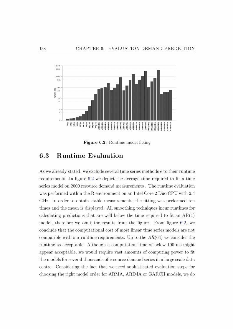
138 CHAPTER 6. EVALUATION DEMAND PREDICTION
AR
(1)
AR
(2)
AR
(4)
AR
(8)
AR
(16)
AR
(32)
AR
(64)
AR
(128
)
AR
(256
)
AR
(512
)
AR
MA
(1,1
)
AR
MA
(1,2
)
AR
MA
(1,4
)
AR
MA
(1,8
)
AR
MA
(2,1
)
AR
MA
(2,2
)
AR
MA
(2,4
)
AR
MA
(2,8
)
AR
MA
(4,1
)
AR
MA
(4,2
)
AR
MA
(4,4
)
AR
MA
(4,8
)
AR
MA
(8,1
)
AR
MA
(8,2
)
AR
MA
(8,4
)
AR
MA
(8,8
)
AR
IMA
(1,1
,1)
AR
IMA
(2,1
,2)
AR
IMA
(4,1
,4)
AR
IMA
(8,1
,8)
GA
RC
H(1
,1)
GA
RC
H(1
,2)
GA
RC
H(2
,1)
GA
RC
H(2
,2)
Run
time
[ms]
1
5
10
50
100
500
1000
5000
10000
50000
1e+05A
R(1
)
AR
(2)
AR
(4)
AR
(8)
AR
(16)
AR
(32)
AR
(64)
AR
(128
)
AR
(256
)
AR
(512
)
AR
MA
(1,1
)
AR
MA
(1,2
)
AR
MA
(1,4
)
AR
MA
(1,8
)
AR
MA
(2,1
)
AR
MA
(2,2
)
AR
MA
(2,4
)
AR
MA
(2,8
)
AR
MA
(4,1
)
AR
MA
(4,2
)
AR
MA
(4,4
)
AR
MA
(4,8
)
AR
MA
(8,1
)
AR
MA
(8,2
)
AR
MA
(8,4
)
AR
MA
(8,8
)
AR
IMA
(1,1
,1)
AR
IMA
(2,1
,2)
AR
IMA
(4,1
,4)
AR
IMA
(8,1
,8)
GA
RC
H(1
,1)
GA
RC
H(1
,2)
GA
RC
H(2
,1)
GA
RC
H(2
,2)
Run
time
[ms]
Figure 6.2: Runtime model fitting
6.3 Runtime Evaluation
As we already stated, we exclude several time series methods e to their runtime
requirements. In figure 6.2 we depict the average time required to fit a time
series model on 2000 resource demand measurements . The runtime evaluation
was performed within the R environment on an Intel Core 2 Duo CPU with 2.4
GHz. In order to obtain stable measurements, the fitting was performed ten
times and the mean is displayed. All smoothing techniques incur runtimes for
calculating predictions that are well below the time required to fit an AR(1)
model, therefore we omit the results from the figure. From figure 6.2, we
conclude that the computational cost of most linear time series models are not
compatible with our runtime requirements. Up to the AR(64) we consider the
runtime as acceptable. Although a computation time of below 100 ms might
appear acceptable, we would require vast amounts of computing power to fit
the models for several thousands of resource demand series in a large scale data
centre. Considering the fact that we need sophisticated evaluation steps for
choosing the right model order for ARMA, ARIMA or GARCH models, we do
6.4. ACCURACY RESULTS 139
not include these models in our study. To avoid model re-fitting, adaptation
logic is required to track the deterioration of the prediction accuracy in order to
decide when a model needs to be re-fitted. Therefore we do not study complex
time series model such as ARMA, ARIMA or GARCH that require complex
parameterization procedures.
6.4 Accuracy Results
We evaluate the smoothing and AR-based forecasting techniques for two CPU
demand data sets: the demand resource traces presented in chapter 4 and
our experimental data sets and evaluate their responsiveness and current load
state estimation (one step ahead forecasts) and predictiveness (3, 6, 12, 24
and 36 steps ahead forecasts). We do so by comparing the RMSE for different
smoothing window sizes and training data window sizes for model fitting. We
compare all prediction models with the last value of the time series and with
a clairvoyant, optimal prediction method that chooses, at each prediction step
the best predictor available by choosing the predictor value that cases the
smallest the forecast error. The following data sets are obtained by applying
all predictors to all time series. The RMSE values for all time series are
collected and the mean and standard deviation are calculated. In the following
subsections we display the results as bar charts: on the y-axis the predictors
are listed in a sorted way, on the x-axis the RMSE is displayed. Each bar gives
the mean RMSE for a predictor, the standard deviation is given by the error
bars.
6.4.1 Consolidation Run Data Results
We present the prediction results for our traces generated during the baseline
consolidation runs of our experiments that we will evaluate in chapter 7. In
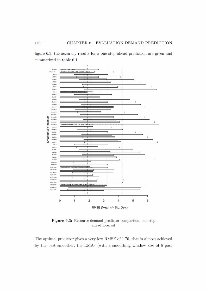
140 CHAPTER 6. EVALUATION DEMAND PREDICTION
figure 6.3, the accuracy results for a one step ahead prediction are given and
summarized in table 6.1.
AR(64) 1024
AR(64) 512
AR(64) 256
AR(32) 1024
AR(32) 512
AR(32) 256
AR(16) 1024
AR(16) 512
AR(16) 256
AR(8) 1024
AR(8) 512
AR(8) 256
SMA 72
SMA 60
SMA 48
SMA 36
SMA 24
SMA 12
SMA 6
QWM 72
QWM 60
QWM 48
QWM 36
QWM 24
QWM 12
QWM 6
Median 72
Median 60
Median 48
Median 36
Median 24
Median 12
Median 6
EMA 72
EMA 60
EMA 48
EMA 36
EMA 24
EMA 12
EMA 6
ATM 72
ATM 60
ATM 48
ATM 36
ATM 24
ATM 12
ATM 6
LAST_VALUE 1
Optimal
Optimal Forecaster vs. Smoother/Forecaster for Lookahead 1
RMSE (Mean +/! Std. Dev.)
Sm
ooth
er/
Fore
caste
r
0 1 2 3 4 5 6
Optimal: 1.7043 ! 100 %
Last Value abs: 2.3538 ! dif to opt: 0.65 ! 138.11 %
Best Smoother abs: 1.8741 ! dif to opt: 0.17 ! 109.96 %
Worst Smoother abs: 4.2575 ! dif to opt: 2.55 ! 249.81 %
Best Forecaster abs: 2.0689 ! dif to opt: 0.36 ! 121.39 %
Worst Forecaster abs: 3.2295 ! dif to opt: 1.53 ! 189.49 %
Figure 6.3: Resource demand predictor comparison, one stepahead forecast
The optimal predictor gives a very low RMSE of 1.70, that is almost achieved
by the best smoother, the EMA6 (with a smoothing window size of 6 past
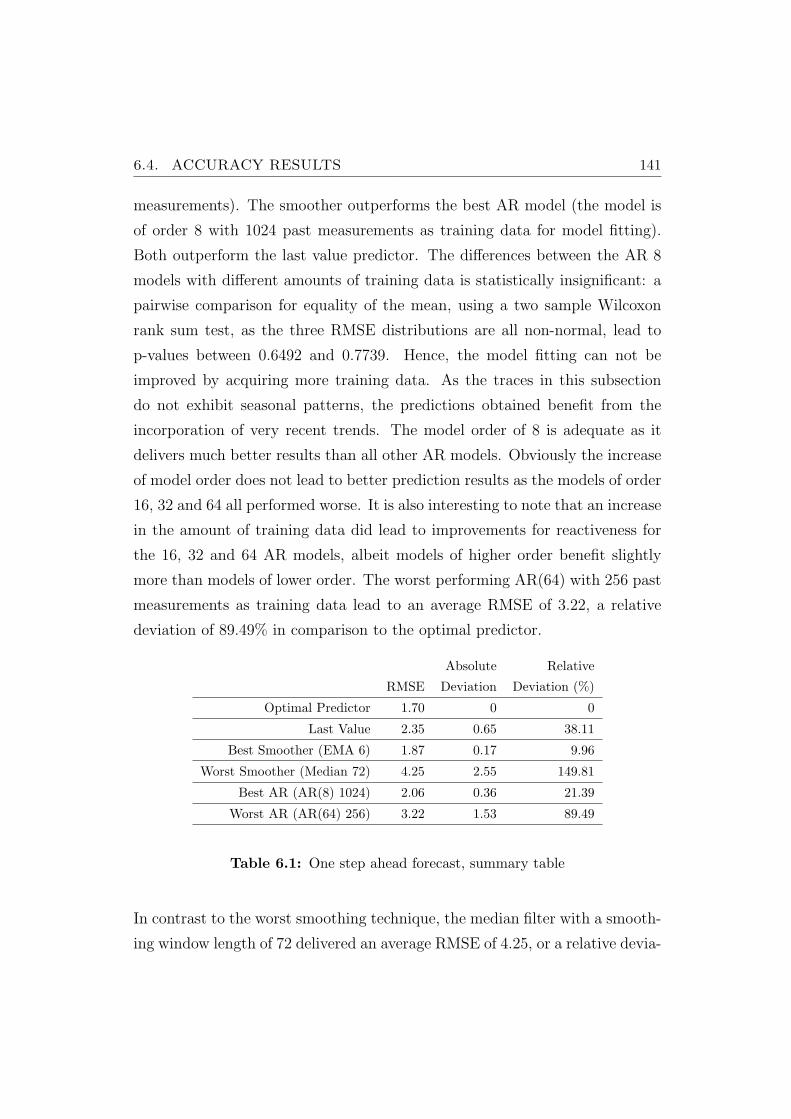
6.4. ACCURACY RESULTS 141
measurements). The smoother outperforms the best AR model (the model is
of order 8 with 1024 past measurements as training data for model fitting).
Both outperform the last value predictor. The differences between the AR 8
models with different amounts of training data is statistically insignificant: a
pairwise comparison for equality of the mean, using a two sample Wilcoxon
rank sum test, as the three RMSE distributions are all non-normal, lead to
p-values between 0.6492 and 0.7739. Hence, the model fitting can not be
improved by acquiring more training data. As the traces in this subsection
do not exhibit seasonal patterns, the predictions obtained benefit from the
incorporation of very recent trends. The model order of 8 is adequate as it
delivers much better results than all other AR models. Obviously the increase
of model order does not lead to better prediction results as the models of order
16, 32 and 64 all performed worse. It is also interesting to note that an increase
in the amount of training data did lead to improvements for reactiveness for
the 16, 32 and 64 AR models, albeit models of higher order benefit slightly
more than models of lower order. The worst performing AR(64) with 256 past
measurements as training data lead to an average RMSE of 3.22, a relative
deviation of 89.49% in comparison to the optimal predictor.
Absolute Relative
RMSE Deviation Deviation (%)
Optimal Predictor 1.70 0 0
Last Value 2.35 0.65 38.11
Best Smoother (EMA 6) 1.87 0.17 9.96
Worst Smoother (Median 72) 4.25 2.55 149.81
Best AR (AR(8) 1024) 2.06 0.36 21.39
Worst AR (AR(64) 256) 3.22 1.53 89.49
Table 6.1: One step ahead forecast, summary table
In contrast to the worst smoothing technique, the median filter with a smooth-
ing window length of 72 delivered an average RMSE of 4.25, or a relative devia-
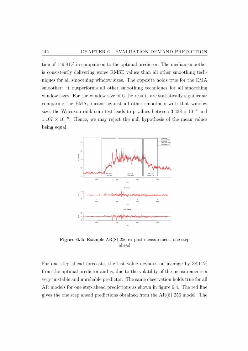
142 CHAPTER 6. EVALUATION DEMAND PREDICTION
tion of 149.81% in comparison to the optimal predictor. The median smoother
is consistently delivering worse RMSE values than all other smoothing tech-
niques for all smoothing window sizes. The opposite holds true for the EMA
smoother: it outperforms all other smoothing techniques for all smoothing
window sizes. For the window size of 6 the results are statistically significant:
comparing the EMA6 means against all other smoothers with that window
size, the Wilcoxon rank sum test leads to p-values between 3.438 × 10⁻⁴ and
1.107 × 10⁻⁹. Hence, we may reject the null hypothesis of the mean values
being equal.Lookahead 1
Time
CP
U D
em
an
d
2000 2200 2400 2600
02
04
06
08
0
Timeseries
Expost SMA 25
AR(8) 256
RMSE Raw: 3.54
RMSE Exp: 3.77
Raw: 3.37
ExPost: 4.2
Raw: 4.66
ExPost: 4.88
Raw: 3.31
ExPost: 3.18
Error Raw
Time
Err
or
2000 2200 2400 2600
!2
00
20
Error Expost
Time
Err
or
2000 2200 2400 2600
!2
00
20
Figure 6.4: Example AR(8) 256 ex-post measurement, one stepahead
For one step ahead forecasts, the last value deviates on average by 38.11%
from the optimal predictor and is, due to the volatility of the measurements a
very unstable and unreliable predictor. The same observation holds true for all
AR models for one step ahead predictions as shown in figure 6.4. The red line
gives the one step ahead predictions obtained from the AR(8) 256 model. The
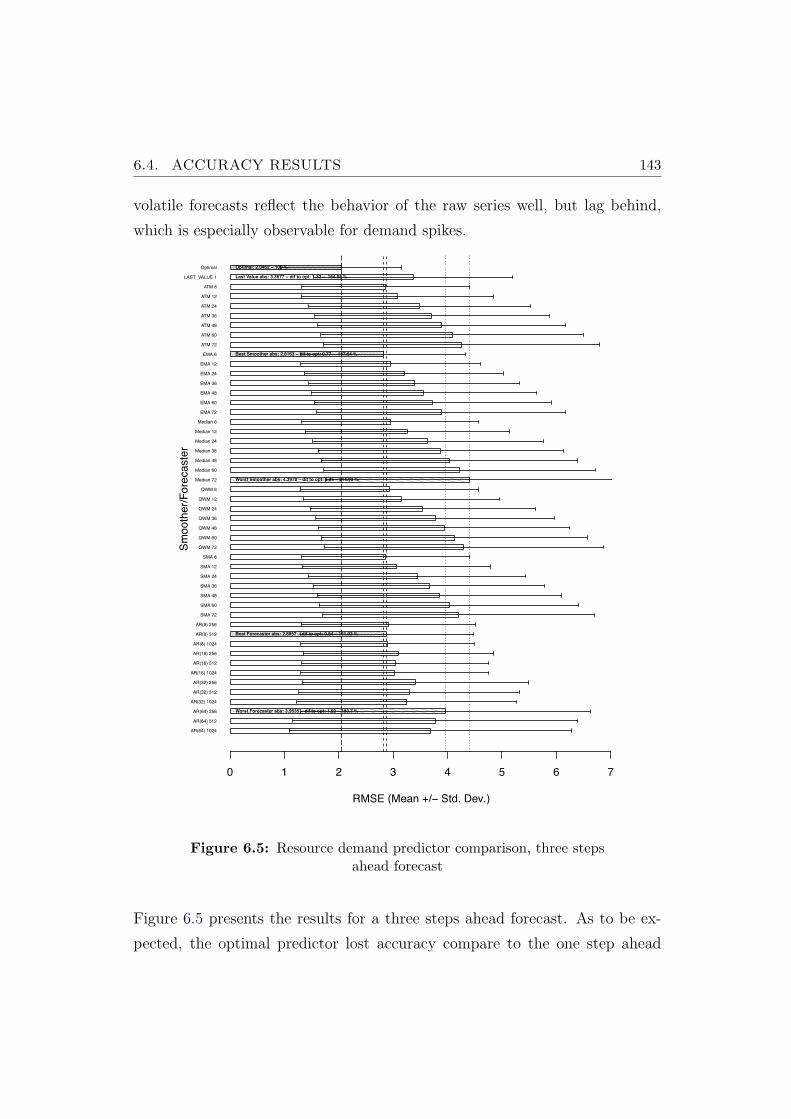
6.4. ACCURACY RESULTS 143
volatile forecasts reflect the behavior of the raw series well, but lag behind,
which is especially observable for demand spikes.
AR(64) 1024
AR(64) 512
AR(64) 256
AR(32) 1024
AR(32) 512
AR(32) 256
AR(16) 1024
AR(16) 512
AR(16) 256
AR(8) 1024
AR(8) 512
AR(8) 256
SMA 72
SMA 60
SMA 48
SMA 36
SMA 24
SMA 12
SMA 6
QWM 72
QWM 60
QWM 48
QWM 36
QWM 24
QWM 12
QWM 6
Median 72
Median 60
Median 48
Median 36
Median 24
Median 12
Median 6
EMA 72
EMA 60
EMA 48
EMA 36
EMA 24
EMA 12
EMA 6
ATM 72
ATM 60
ATM 48
ATM 36
ATM 24
ATM 12
ATM 6
LAST_VALUE 1
Optimal
Optimal Forecaster vs. Smoother/Forecaster for Lookahead 3
RMSE (Mean +/! Std. Dev.)
Sm
ooth
er/
Fore
caste
r
0 1 2 3 4 5 6 7
Optimal: 2.0462 ! 100 %
Last Value abs: 3.3677 ! dif to opt: 1.32 ! 164.58 %
Best Smoother abs: 2.8163 ! dif to opt: 0.77 ! 137.64 %
Worst Smoother abs: 4.3978 ! dif to opt: 2.35 ! 214.93 %
Best Forecaster abs: 2.8857 ! dif to opt: 0.84 ! 141.03 %
Worst Forecaster abs: 3.9635 ! dif to opt: 1.92 ! 193.7 %
Figure 6.5: Resource demand predictor comparison, three stepsahead forecast
Figure 6.5 presents the results for a three steps ahead forecast. As to be ex-
pected, the optimal predictor lost accuracy compare to the one step ahead
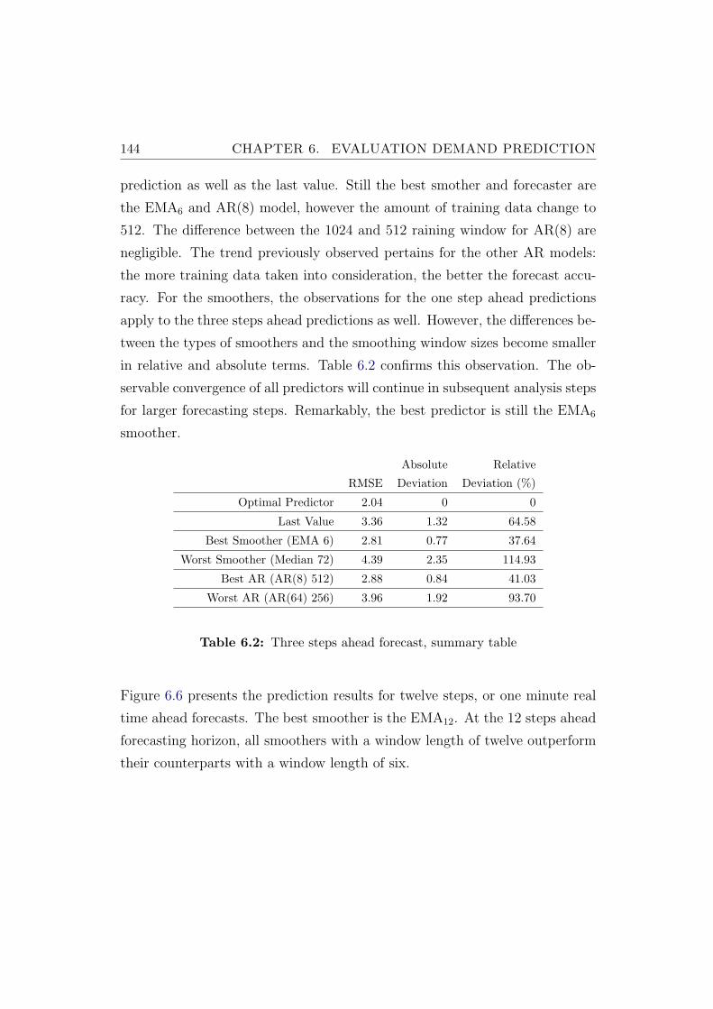
144 CHAPTER 6. EVALUATION DEMAND PREDICTION
prediction as well as the last value. Still the best smother and forecaster are
the EMA6 and AR(8) model, however the amount of training data change to
512. The difference between the 1024 and 512 raining window for AR(8) are
negligible. The trend previously observed pertains for the other AR models:
the more training data taken into consideration, the better the forecast accu-
racy. For the smoothers, the observations for the one step ahead predictions
apply to the three steps ahead predictions as well. However, the differences be-
tween the types of smoothers and the smoothing window sizes become smaller
in relative and absolute terms. Table 6.2 confirms this observation. The ob-
servable convergence of all predictors will continue in subsequent analysis steps
for larger forecasting steps. Remarkably, the best predictor is still the EMA6
smoother.
Absolute Relative
RMSE Deviation Deviation (%)
Optimal Predictor 2.04 0 0
Last Value 3.36 1.32 64.58
Best Smoother (EMA 6) 2.81 0.77 37.64
Worst Smoother (Median 72) 4.39 2.35 114.93
Best AR (AR(8) 512) 2.88 0.84 41.03
Worst AR (AR(64) 256) 3.96 1.92 93.70
Table 6.2: Three steps ahead forecast, summary table
Figure 6.6 presents the prediction results for twelve steps, or one minute real
time ahead forecasts. The best smoother is the EMA12. At the 12 steps ahead
forecasting horizon, all smoothers with a window length of twelve outperform
their counterparts with a window length of six.
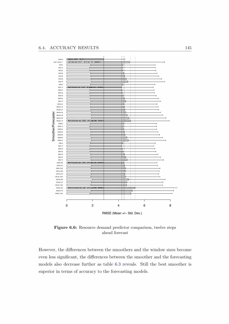
6.4. ACCURACY RESULTS 145
AR(64) 1024
AR(64) 512
AR(64) 256
AR(32) 1024
AR(32) 512
AR(32) 256
AR(16) 1024
AR(16) 512
AR(16) 256
AR(8) 1024
AR(8) 512
AR(8) 256
SMA 72
SMA 60
SMA 48
SMA 36
SMA 24
SMA 12
SMA 6
QWM 72
QWM 60
QWM 48
QWM 36
QWM 24
QWM 12
QWM 6
Median 72
Median 60
Median 48
Median 36
Median 24
Median 12
Median 6
EMA 72
EMA 60
EMA 48
EMA 36
EMA 24
EMA 12
EMA 6
ATM 72
ATM 60
ATM 48
ATM 36
ATM 24
ATM 12
ATM 6
LAST_VALUE 1
Optimal
Optimal Forecaster vs. Smoother/Forecaster for Lookahead 12
RMSE (Mean +/! Std. Dev.)
Sm
ooth
er/
Fore
caste
r
0 2 4 6 8
Optimal: 2.8674 ! 100 %
Last Value abs: 4.8571 ! dif to opt: 1.99 ! 169.39 %
Best Smoother abs: 4.2394 ! dif to opt: 1.37 ! 147.85 %
Worst Smoother abs: 4.9322 ! dif to opt: 2.06 ! 172.01 %
Best Forecaster abs: 4.4375 ! dif to opt: 1.57 ! 154.76 %
Worst Forecaster abs: 5.287 ! dif to opt: 2.42 ! 184.38 %
Figure 6.6: Resource demand predictor comparison, twelve stepsahead forecast
However, the differences between the smoothers and the window sizes become
even less significant, the differences between the smoother and the forecasting
models also decrease further as table 6.3 reveals. Still the best smoother is
superior in terms of accuracy to the forecasting models.
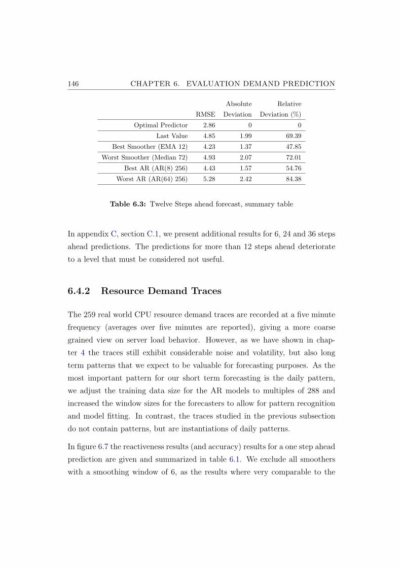
146 CHAPTER 6. EVALUATION DEMAND PREDICTION
Absolute Relative
RMSE Deviation Deviation (%)
Optimal Predictor 2.86 0 0
Last Value 4.85 1.99 69.39
Best Smoother (EMA 12) 4.23 1.37 47.85
Worst Smoother (Median 72) 4.93 2.07 72.01
Best AR (AR(8) 256) 4.43 1.57 54.76
Worst AR (AR(64) 256) 5.28 2.42 84.38
Table 6.3: Twelve Steps ahead forecast, summary table
In appendix C, section C.1, we present additional results for 6, 24 and 36 steps
ahead predictions. The predictions for more than 12 steps ahead deteriorate
to a level that must be considered not useful.
6.4.2 Resource Demand Traces
The 259 real world CPU resource demand traces are recorded at a five minute
frequency (averages over five minutes are reported), giving a more coarse
grained view on server load behavior. However, as we have shown in chap-
ter 4 the traces still exhibit considerable noise and volatility, but also long
term patterns that we expect to be valuable for forecasting purposes. As the
most important pattern for our short term forecasting is the daily pattern,
we adjust the training data size for the AR models to multiples of 288 and
increased the window sizes for the forecasters to allow for pattern recognition
and model fitting. In contrast, the traces studied in the previous subsection
do not contain patterns, but are instantiations of daily patterns.
In figure 6.7 the reactiveness results (and accuracy) results for a one step ahead
prediction are given and summarized in table 6.1. We exclude all smoothers
with a smoothing window of 6, as the results where very comparable to the
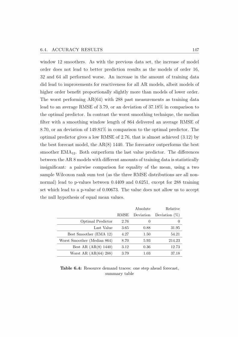
6.4. ACCURACY RESULTS 147
window 12 smoothers. As with the previous data set, the increase of model
order does not lead to better prediction results as the models of order 16,
32 and 64 all performed worse. An increase in the amount of training data
did lead to improvements for reactiveness for all AR models, albeit models of
higher order benefit proportionally slightly more than models of lower order.
The worst performing AR(64) with 288 past measurements as training data
lead to an average RMSE of 3.79, or an deviation of 37.18% in comparison to
the optimal predictor. In contrast the worst smoothing technique, the median
filter with a smoothing window length of 864 delivered an average RMSE of
8.70, or an deviation of 149.81% in comparison to the optimal predictor. The
optimal predictor gives a low RMSE of 2.76, that is almost achieved (3.12) by
the best forecast model, the AR(8) 1440. The forecaster outperforms the best
smoother EMA12. Both outperform the last value predictor. The differences
between the AR 8 models with different amounts of training data is statistically
insignificant: a pairwise comparison for equality of the mean, using a two
sample Wilcoxon rank sum test (as the three RMSE distributions are all non-
normal) lead to p-values between 0.4409 and 0.6251, except for 288 training
set which lead to a p-value of 0.00673. The value does not allow us to accept
the null hypothesis of equal mean values.
Absolute Relative
RMSE Deviation Deviation (%)
Optimal Predictor 2.76 0 0
Last Value 3.65 0.88 31.95
Best Smoother (EMA 12) 4.27 1.50 54.21
Worst Smoother (Median 864) 8.70 5.93 214.23
Best AR (AR(8) 1440) 3.12 0.36 12.73
Worst AR (AR(64) 288) 3.79 1.03 37.18
Table 6.4: Resource demand traces: one step ahead forecast,summary table
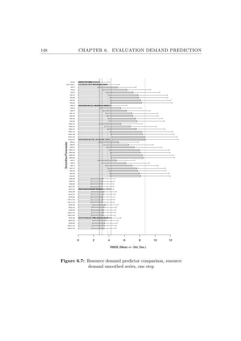
148 CHAPTER 6. EVALUATION DEMAND PREDICTION
AR(64) 1440
AR(64) 1152
AR(64) 864
AR(64) 576
AR(64) 288
AR(32) 1440
AR(32) 1152
AR(32) 864
AR(32) 576
AR(32) 288
AR(16) 1440
AR(16) 1152
AR(16) 864
AR(16) 576
AR(16) 288
AR(8) 1440
AR(8) 1152
AR(8) 864
AR(8) 576
AR(8) 288
SMA 864
SMA 576
SMA 288
SMA 144
SMA 72
SMA 36
SMA 12
QWM 864
QWM 576
QWM 288
QWM 144
QWM 72
QWM 36
QWM 12
Median 864
Median 576
Median 288
Median 144
Median 72
Median 36
Median 12
EMA 864
EMA 576
EMA 288
EMA 144
EMA 72
EMA 36
EMA 12
ATM 864
ATM 576
ATM 288
ATM 144
ATM 72
ATM 36
ATM 12
LAST_VALUE 1
Optimal
Optimal Forecaster vs. Smoother/Forecaster for Lookahead 1
RMSE (Mean +/! Std. Dev.)
Sm
oo
the
r/F
ore
ca
ste
r
0 2 4 6 8 10 12
Optimal: 2.769 ! 100 %
Last Value abs: 3.6539 ! dif to opt: 0.88 ! 131.96 %
Best Smoother abs: 4.27 ! dif to opt: 1.5 ! 154.21 %
Worst Smoother abs: 8.701 ! dif to opt: 5.93 ! 314.23 %
Best Forecaster abs: 3.1216 ! dif to opt: 0.35 ! 112.73 %
Worst Forecaster abs: 3.7986 ! dif to opt: 1.03 ! 137.18 %
Figure 6.7: Resource demand predictor comparison, resourcedemand smoothed series, one step
6.4. ACCURACY RESULTS 149
Again, the median smoother is consistently delivering worse RMSE values
than all other smoothing techniques for all smoothing window sizes. The
opposite holds true for the EMA smoother. It outperforms all other smoothing
techniques for all smoothing window sizes. For the window size of six, the
results are statistically significant. Comparing the EMA12 means against all
other smoothers with that window size, the Wilcoxon rank sum test leads to
p-values between 1.855×10⁻¹⁶ and 2.054×10⁻¹⁸. We reject the null hypothesis
of the mean values being equal. In contrast to the findings for the previous
data set, the forecaster are more reactive than the smoothers, hat is, they
adapt quicker to changes in the demands.
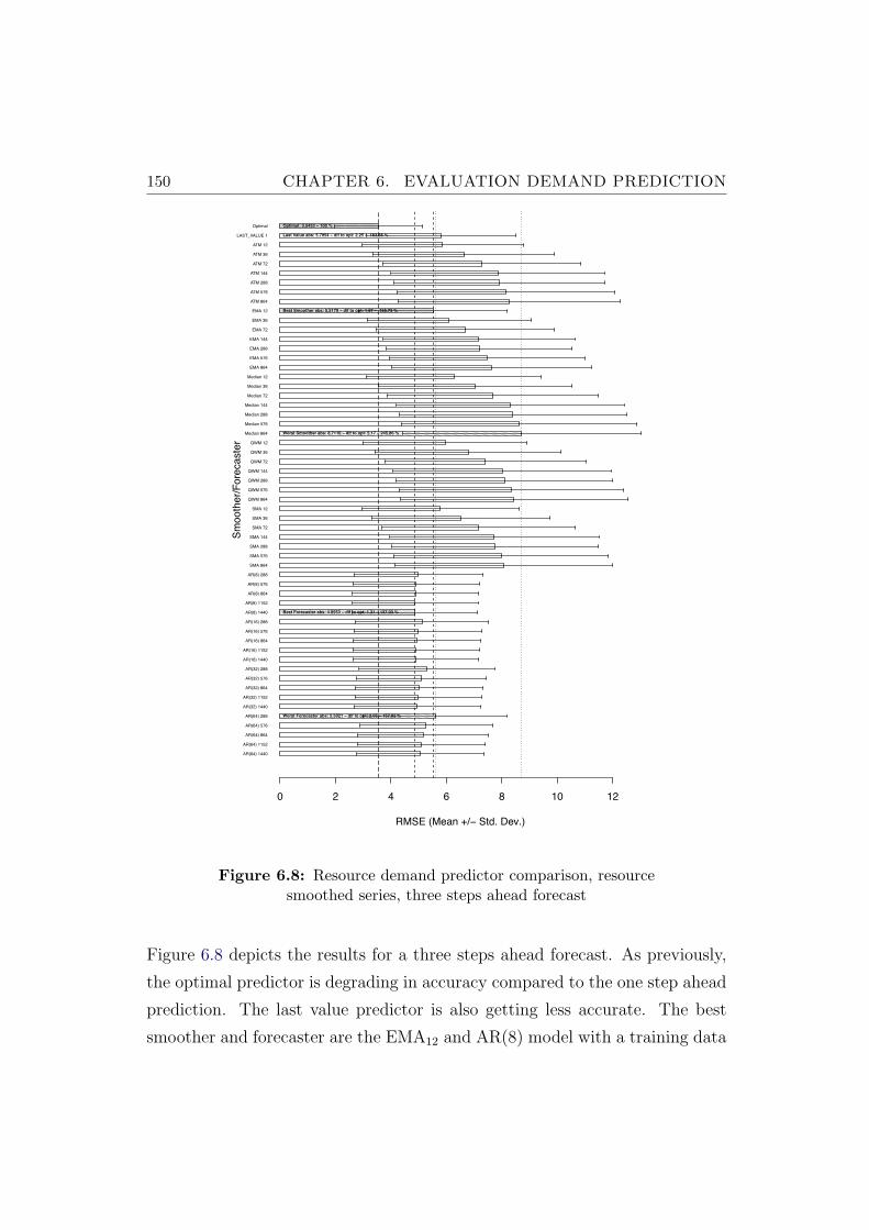
150 CHAPTER 6. EVALUATION DEMAND PREDICTION
AR(64) 1440
AR(64) 1152
AR(64) 864
AR(64) 576
AR(64) 288
AR(32) 1440
AR(32) 1152
AR(32) 864
AR(32) 576
AR(32) 288
AR(16) 1440
AR(16) 1152
AR(16) 864
AR(16) 576
AR(16) 288
AR(8) 1440
AR(8) 1152
AR(8) 864
AR(8) 576
AR(8) 288
SMA 864
SMA 576
SMA 288
SMA 144
SMA 72
SMA 36
SMA 12
QWM 864
QWM 576
QWM 288
QWM 144
QWM 72
QWM 36
QWM 12
Median 864
Median 576
Median 288
Median 144
Median 72
Median 36
Median 12
EMA 864
EMA 576
EMA 288
EMA 144
EMA 72
EMA 36
EMA 12
ATM 864
ATM 576
ATM 288
ATM 144
ATM 72
ATM 36
ATM 12
LAST_VALUE 1
Optimal
Optimal Forecaster vs. Smoother/Forecaster for Lookahead 3
RMSE (Mean +/! Std. Dev.)
Sm
oo
the
r/F
ore
ca
ste
r
0 2 4 6 8 10 12
Optimal: 3.5433 ! 100 %
Last Value abs: 5.7954 ! dif to opt: 2.25 ! 163.56 %
Best Smoother abs: 5.5179 ! dif to opt: 1.97 ! 155.73 %
Worst Smoother abs: 8.7116 ! dif to opt: 5.17 ! 245.86 %
Best Forecaster abs: 4.8553 ! dif to opt: 1.31 ! 137.03 %
Worst Forecaster abs: 5.5921 ! dif to opt: 2.05 ! 157.82 %
Figure 6.8: Resource demand predictor comparison, resourcesmoothed series, three steps ahead forecast
Figure 6.8 depicts the results for a three steps ahead forecast. As previously,
the optimal predictor is degrading in accuracy compared to the one step ahead
prediction. The last value predictor is also getting less accurate. The best
smoother and forecaster are the EMA12 and AR(8) model with a training data
6.4. ACCURACY RESULTS 151
size of 1440. For three steps ahead, the predictiveness of all forecasters suf-
fered proportionally. However in comparison to the smoothers, the forecasters
degraded much more. The best smoother outperforms the worst forecaster.
For the other AR models the trend previously observed pertains: the more
training data taken into consideration, the better the forecast accuracy. For
the smoothers, the observations for the one step ahead predictions apply to
the three steps ahead predictions as well. However, the differences between the
types of smoothers and the smoothing window sizes become smaller in relative
and absolute terms. Table 6.5 confirms this observation. The observable con-
vergence of all predictors will continue in subsequent analysis steps for larger
forecasting steps. The convergence will be even more pronounced than for the
first data set. Remarkably, the best predictor is the EMA12 smoother.
Absolute Relative
RMSE Deviation Deviation (%)
Optimal Predictor 3.54 0 0
Last Value 5.79 2.25 63.56
Best Smoother (EMA 12) 5.51 1.97 55.73
Worst Smoother (Median 864) 8.71 5.17 145.86
Best AR (AR(8) 1440) 4.85 1.31 37.03
Worst AR (AR(64) 288) 5.59 2.05 57.82
Table 6.5: Resource demand traces: three steps ahead forecast,summary table
Figure 6.9 presents the prediction results for 12 steps ahead. The best
smoothers still are the EMA, ATM, SMA and QMA filters with a smooth-
ing window size of 12.
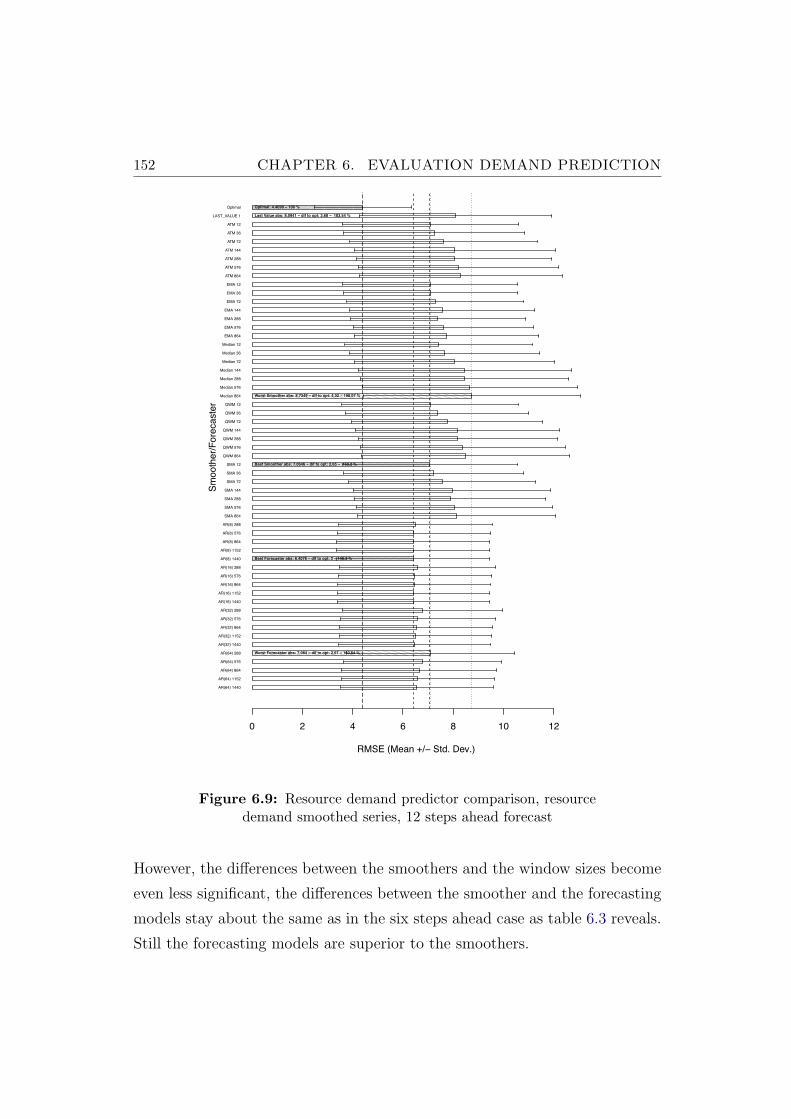
152 CHAPTER 6. EVALUATION DEMAND PREDICTION
AR(64) 1440
AR(64) 1152
AR(64) 864
AR(64) 576
AR(64) 288
AR(32) 1440
AR(32) 1152
AR(32) 864
AR(32) 576
AR(32) 288
AR(16) 1440
AR(16) 1152
AR(16) 864
AR(16) 576
AR(16) 288
AR(8) 1440
AR(8) 1152
AR(8) 864
AR(8) 576
AR(8) 288
SMA 864
SMA 576
SMA 288
SMA 144
SMA 72
SMA 36
SMA 12
QWM 864
QWM 576
QWM 288
QWM 144
QWM 72
QWM 36
QWM 12
Median 864
Median 576
Median 288
Median 144
Median 72
Median 36
Median 12
EMA 864
EMA 576
EMA 288
EMA 144
EMA 72
EMA 36
EMA 12
ATM 864
ATM 576
ATM 288
ATM 144
ATM 72
ATM 36
ATM 12
LAST_VALUE 1
Optimal
Optimal Forecaster vs. Smoother/Forecaster for Lookahead 9
RMSE (Mean +/! Std. Dev.)
Sm
oo
the
r/F
ore
ca
ste
r
0 2 4 6 8 10 12
Optimal: 4.4099 ! 100 %
Last Value abs: 8.0941 ! dif to opt: 3.68 ! 183.54 %
Best Smoother abs: 7.0646 ! dif to opt: 2.65 ! 160.2 %
Worst Smoother abs: 8.7349 ! dif to opt: 4.32 ! 198.07 %
Best Forecaster abs: 6.4076 ! dif to opt: 2 ! 145.3 %
Worst Forecaster abs: 7.084 ! dif to opt: 2.67 ! 160.64 %
Figure 6.9: Resource demand predictor comparison, resourcedemand smoothed series, 12 steps ahead forecast
However, the differences between the smoothers and the window sizes become
even less significant, the differences between the smoother and the forecasting
models stay about the same as in the six steps ahead case as table 6.3 reveals.
Still the forecasting models are superior to the smoothers.
6.5. INSIGHTS GAINED 153
Absolute Relative
RMSE Deviation Deviation (%)
Optimal Predictor 4.40 0 0
Last Value 8.09 3.68 83.54
Best Smoother (SMA 12) 7.06 2.65 60.20
Worst Smoother (Median 864) 8.73 4.32 98.07
Best AR (AR(8) 1440) 6.40 2.00 45.30
Worst AR (AR(64) 288) 7.08 2.67 60.54
Table 6.6: Resource demand traces: twelve steps ahead forecast,summary table
In appendix C, section C.2, we present additional results for 6, 24 and 36 steps
ahead predictions. The predictions for more than 12 steps ahead deteriorate
to a level that can be considered not useful anymore. For longer prediction
windows, the accuracy of all predictors becomes unreliably and chance-driven.
6.5 Insights Gained
We evaluated short term resource demand estimation techniques that have
been proposed in the literature for two distinct data sets. We found that it
is possible to predict the resource demands for typical enterprise applications
up to twelve steps ahead of time for both data sets with acceptable prediction
accuracy. Predicting high frequency time series that expose highly volatile
behavior is feasible for short forecasting horizons by applying the selected
techniques and methods. Forecasts for longer horizons are difficult even if
strong, recurring patterns exist. While we can not preclude the existence of
better techniques, we have shown that it may be hard to improve upon the best
currently known estimation techniques given the highly volatile and uncertain
environment. The convergence process observed for all predictors and data
sets indicates that it is not possible to adjust the prediction methods.
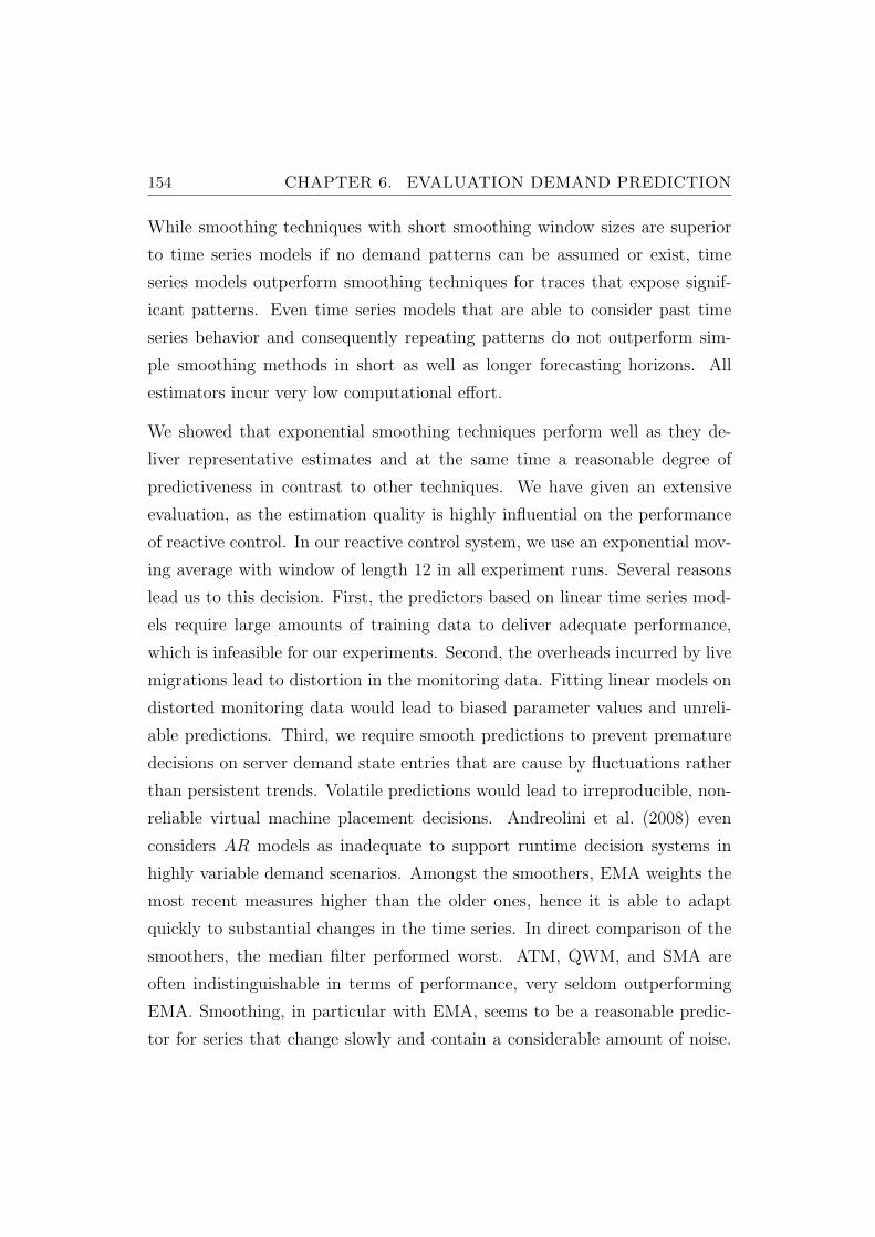
154 CHAPTER 6. EVALUATION DEMAND PREDICTION
While smoothing techniques with short smoothing window sizes are superior
to time series models if no demand patterns can be assumed or exist, time
series models outperform smoothing techniques for traces that expose signif-
icant patterns. Even time series models that are able to consider past time
series behavior and consequently repeating patterns do not outperform sim-
ple smoothing methods in short as well as longer forecasting horizons. All
estimators incur very low computational effort.
We showed that exponential smoothing techniques perform well as they de-
liver representative estimates and at the same time a reasonable degree of
predictiveness in contrast to other techniques. We have given an extensive
evaluation, as the estimation quality is highly influential on the performance
of reactive control. In our reactive control system, we use an exponential mov-
ing average with window of length 12 in all experiment runs. Several reasons
lead us to this decision. First, the predictors based on linear time series mod-
els require large amounts of training data to deliver adequate performance,
which is infeasible for our experiments. Second, the overheads incurred by live
migrations lead to distortion in the monitoring data. Fitting linear models on
distorted monitoring data would lead to biased parameter values and unreli-
able predictions. Third, we require smooth predictions to prevent premature
decisions on server demand state entries that are cause by fluctuations rather
than persistent trends. Volatile predictions would lead to irreproducible, non-
reliable virtual machine placement decisions. Andreolini et al. (2008) even
considers AR models as inadequate to support runtime decision systems in
highly variable demand scenarios. Amongst the smoothers, EMA weights the
most recent measures higher than the older ones, hence it is able to adapt
quickly to substantial changes in the time series. In direct comparison of the
smoothers, the median filter performed worst. ATM, QWM, and SMA are
often indistinguishable in terms of performance, very seldom outperforming
EMA. Smoothing, in particular with EMA, seems to be a reasonable predic-
tor for series that change slowly and contain a considerable amount of noise.
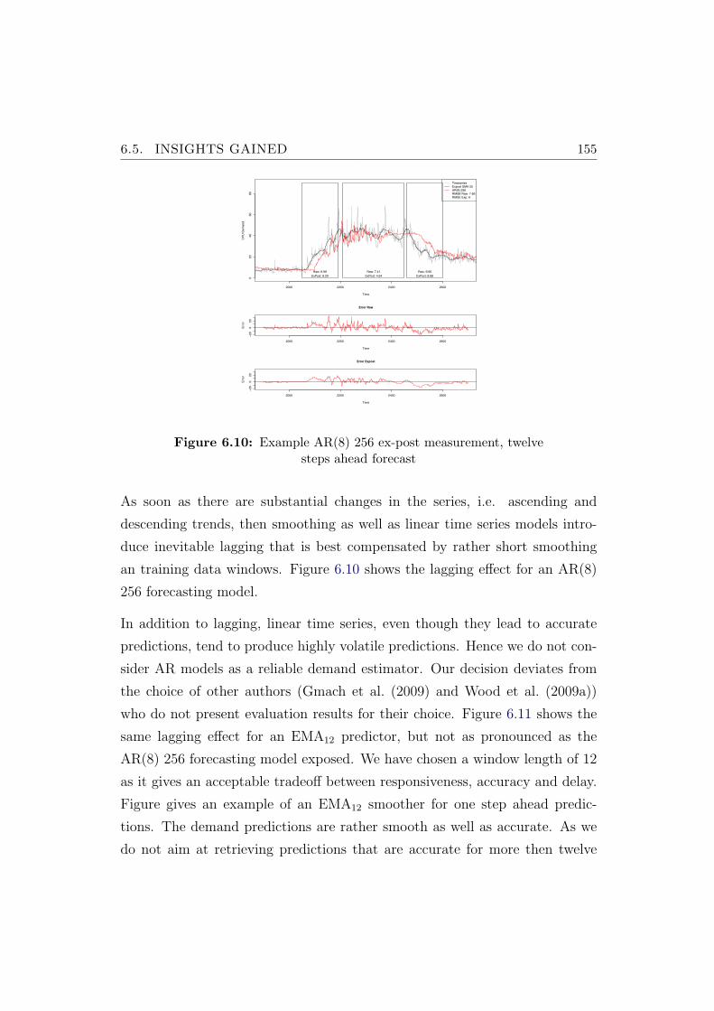
6.5. INSIGHTS GAINED 155Lookahead 12
Time
CP
U D
em
and
2000 2200 2400 2600
020
40
60
80
Timeseries
Expost SMA 25
AR(8) 256
RMSE Raw: 7.66
RMSE Exp: 6
Raw: 9.99
ExPost: 8.29
Raw: 7.41
ExPost: 4.64
Raw: 9.66
ExPost: 8.88
Error Raw
Time
Err
or
2000 2200 2400 2600
!20
020
Error Expost
Time
Err
or
2000 2200 2400 2600
!20
020
Figure 6.10: Example AR(8) 256 ex-post measurement, twelvesteps ahead forecast
As soon as there are substantial changes in the series, i.e. ascending and
descending trends, then smoothing as well as linear time series models intro-
duce inevitable lagging that is best compensated by rather short smoothing
an training data windows. Figure 6.10 shows the lagging effect for an AR(8)
256 forecasting model.
In addition to lagging, linear time series, even though they lead to accurate
predictions, tend to produce highly volatile predictions. Hence we do not con-
sider AR models as a reliable demand estimator. Our decision deviates from
the choice of other authors (Gmach et al. (2009) and Wood et al. (2009a))
who do not present evaluation results for their choice. Figure 6.11 shows the
same lagging effect for an EMA12 predictor, but not as pronounced as the
AR(8) 256 forecasting model exposed. We have chosen a window length of 12
as it gives an acceptable tradeoff between responsiveness, accuracy and delay.
Figure gives an example of an EMA12 smoother for one step ahead predic-
tions. The demand predictions are rather smooth as well as accurate. As we
do not aim at retrieving predictions that are accurate for more then twelve
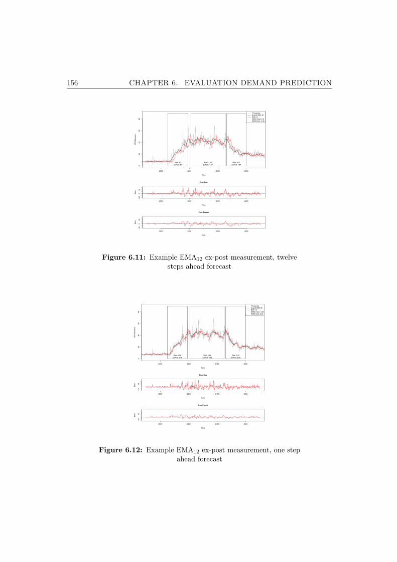
156 CHAPTER 6. EVALUATION DEMAND PREDICTION
Lookahead 12
Time
CP
U D
em
and
2000 2200 2400 2600
020
40
60
80
Timeseries
Expost SMA 25
EMA 12
RMSE Raw: 6.6
RMSE Exp: 4.46
Raw: 8.2
ExPost: 5.9
Raw: 7.33
ExPost: 4.48
Raw: 6.12
ExPost: 4.84
Error Raw
Time
Err
or
2000 2200 2400 2600
!20
020
Error Expost
Time
Err
or
2000 2200 2400 2600
!20
020
Figure 6.11: Example EMA12 ex-post measurement, twelvesteps ahead forecast
Lookahead 1
Time
CP
U D
em
and
2000 2200 2400 2600
020
40
60
80
Timeseries
Expost SMA 25
EMA 12
RMSE Raw: 4.65
RMSE Exp: 2.24
Raw: 5.06
ExPost: 3.19
Raw: 5.95
ExPost: 2.52
Raw: 3.92
ExPost: 2.09
Error Raw
Time
Err
or
2000 2200 2400 2600
!10
10
Error Expost
Time
Err
or
2000 2200 2400 2600
!10
10
Figure 6.12: Example EMA12 ex-post measurement, one stepahead forecast
6.5. INSIGHTS GAINED 157
steps ahead of time, the EMA is the best choice for our purposes. Linear time
series models are often adopted for workload representation and estimation.
Our findings are in accordance with Cherkasova and Phaal (2002) who show
that the exponential moving average of the CPU demand can be used as a
valid predictor for web server workloads, as well as Andreolini et al. (2008).
The authors evaluate various smoothing techniques and auto-regressive time
series models to obtain a representative, instantaneous view of the resource
utilization trends from high frequency monitoring data and apply this repre-
sentation to support runtime decision systems such as admission control and
load balancing. Their study shows that even simple smoothing methods like
exponential moving averages have a computational cost that is compatible
with runtime constraints and that one step ahead predictions can be done us-
ing the smoothing techniques. Their findings deliver empirical evidence that
EMA techniques are feasible even on small window sizes and deliver an ac-
ceptable trade-off between responsiveness and accuracy. In contrast, Dinda
and O’Hallaron (2000) propose linear models on CPU demand traces gath-
ered from productive physical servers operating in a grid environment. Their
results show that the simple auto-regressive model exposes good predictive
power. However these methods, as shown in Andreolini et al. (2008) are not
well suited for highly volatile resource demands and result in rather noised
predictions which reduce the predictive power of auto-regressive models and
may lead to wrong control decisions in threshold based control strategies.
In summary, we have shown that very simple smoothing methods are rea-
sonable for predicting the resource utilization in highly volatile environments.
Our work on resource demand prediction is closest to Andreolini et al. (2008),
however we use different and real world data sets to evaluate the predictive
power of simple time series methods and focus on techniques that can be used
in large enterprise data centres. An issue with simple prediction techniques,
even for highly reactive ones, is latency and responsiveness of the predictions.
Chapter 7
Reactive Control System
Evaluation
Better to be alone than in bad company
by George Washington
Our main interest is the analysis of the performance of our reactive control
system and the impact of different control system parameters using a set of
generated benchmark scenarios that vary in the amount of virtual machines
deployed into the infrastructure, their resource demands relative to the ca-
pacity of the physical servers and the time-varying service demands. We first
describe the experimental set-up before we present an analysis of the obtained
results, give a discussion on the insights gained and provide a short conclusion.
Due to the sometimes limited amount of data, we will rely on statistical tests
to underpin our findings with statistical significance.
All our experiments for reactive control are run using the EMA12 filter as it
gives an acceptable tradeoff between responsiveness and accuracy. All experi-
ments have been executed with the same resource allocation for domain0 : It
158

7.1. EXPERIMENTAL DESIGN 159
has 512 MB of main memory allocated and a single virtual CPU. This allo-
cation has proven to be reasonable and never lead to memory shortages for
domain0.
To clarify on our nomenclature, we introduce several terms we will use fre-
quently in subsequent subsections:
• A scenario is a set of virtual machines with time dependent service de-
mands and a conservative, baseline consolidation plan that utilizes all
six SUT physical servers.
• An experiment is a scenario in combination with a control system pa-
rameter configuration. To uniquely identify a control parameter config-
uration, we introduce the notation: (Placement Strategy/Lower Thresh-
old/Upper Threshold/Detection Delay); E.g. an experiment with an up-
per threshold of 75, lower threshold of 20, a detection delay of 12 control
cycles and a best fit placement strategy is denoted as (BF/20/75/12).
• An experiment run is the execution of an experiment. An experiment
may be executed several times. The execution of a baseline consolidation
plan is called baseline consolidation run.
• In the subsection 7.6 on overbooking we reduce the number of servers
available for a base consolidation plan. These plans will be denoted
by x% overbooked consolidation plans, where x is the amount to the
reduction of available servers in %.
7.1 Experimental Design
Overall, we include 215 experiment runs with 13 different benchmark scenarios
into our analysis. For 9 scenarios we executed a full set of treatments, while
4 scenarios served us for initial testing purposes and to determine relevant
160 CHAPTER 7. REACTIVE CONTROL SYSTEM EVALUATION
treatments to study. We therefore include only valid experiment runs for these
3 scenarios. For each experiment we executed two experiment runs.
The treatments we test are:
• Upper CPU thresholds ∈ {75, 85}
• Lower CPU thresholds ∈ {20, 30}
• Detection delay ∈ {1, 6, 12, 24, 36}
• Virtual machine placement strategy ∈ {BF,WF}
As a full coverage of all treatments would have required 960 experiments, each
requiring about 16 hours on average, including infrastructure setup, initial-
ization and tear down and post processing time, which would have resulted
in 640 days experimental time, we reduced the treatment combinations. The
experiment groups are listed in table 7.1.
For each scenario we executed experiments with lower and upper thresholds of
30 and 75% respectively and detection delay of 1 for both placement strategies.
This requires 4 experiment runs for each scenario. We executed these two
experiments for all scenarios leading to 13 = 52 experiment runs (experiment
groups 1 and 2).
We then executed experiments with the worst fit placement strategy for all
remaining detection delays (6, 12, 24, 36) for the same threshold values which
required another 8 runs per scenario, which required 9 × 8 = 72 experiment
runs (experiment groups 3 to 6). We excluded four scenarios that exhibited
very similar behavior to other scenarios due to time constraints.
Experiment groups 7 was setup to provide a fair comparison of the worst fit
with the best fit placement strategy using the detection delay that provided
the best results for each scenario in terms of average response time (detection
7.1. EXPERIMENTAL DESIGN 161
delay OPT ). This required another 9×2 = 18 experiment runs for experiment
group 7, employing the best fit placement strategy for 9 scenarios.
We then executed, with a detection delay of one, an experiment with lower
and upper threshold of 20 and 75% and the worst fit placement strategy as
well as an experiment with the best detection delay for the 9 scenarios, which
required another 9× 4 = 36 experiment runs (experiment groups 8 and 9).
To test the influence of the upper threshold we executed an experiment with
detection delay one and an experiment with the best detection delay on seven,
respectively six hand-picked scenarios resulting in 14 + 12 = 26 experiment
runs (experiment groups 10 and 11).
The remaining experiments were used to test the influence of virtual machine
swaps and to test a tentative controller. We hand-picked two scenarios, and
executed experiments with the worst fit placement strategy, upper and lower
thresholds of 30/75 and different detection delays requiring seven experiment
runs (experiment groups 12 and 13) in sum. For the tentative controller tests
we executed four experiment runs for two hand-selected scenarios (experiment
group 14). We will refer to the experiment groups in the following sections to
point out which experiment runs were used in the statistical analyses.
Overall, we executed 215 experiment runs with the control systems enabled and
36 as static consolidation runs without the control system. The time required
was more than seven months. Even though we executed the experiments in
a fully automated way, we were not able to execute more experiments, as we
had to discard several runs due to hardware defects, network outages and most
often failed live migrations caused by errors in the hypervisor layer.
For all consolidation runs we set the usable resource capacities to 98.5% for
main memory and 85% for CPU. We consider 15% CPU capacity to be a
reasonable buffer. We used the same settings to calculate the expectation
baselines for the scenarios. All reactive control experiments were started with
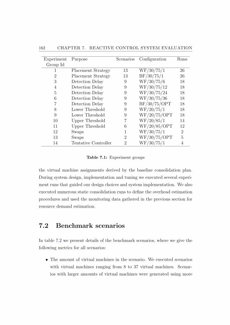
162 CHAPTER 7. REACTIVE CONTROL SYSTEM EVALUATION
Experiment Purpose Scenarios Configuration RunsGroup Id
1 Placement Strategy 13 WF/30/75/1 262 Placement Strategy 13 BF/30/75/1 263 Detection Delay 9 WF/30/75/6 184 Detection Delay 9 WF/30/75/12 185 Detection Delay 9 WF/30/75/24 186 Detection Delay 9 WF/30/75/36 187 Detection Delay 9 BF/30/75/OPT 188 Lower Threshold 9 WF/20/75/1 189 Lower Threshold 9 WF/20/75/OPT 1810 Upper Threshold 7 WF/20/85/1 1411 Upper Threshold 6 WF/20/85/OPT 1212 Swaps 1 WF/30/75/1 213 Swaps 2 WF/30/75/OPT 514 Tentative Controller 2 WF/30/75/1 4
Table 7.1: Experiment groups
the virtual machine assignments derived by the baseline consolidation plan.
During system design, implementation and tuning we executed several experi-
ment runs that guided our design choices and system implementation. We also
executed numerous static consolidation runs to define the overhead estimation
procedures and used the monitoring data gathered in the previous section for
resource demand estimation.
7.2 Benchmark scenarios
In table 7.2 we present details of the benchmark scenarios, where we give the
following metrics for all scenarios:
• The amount of virtual machines in the scenario. We executed scenarios
with virtual machines ranging from 8 to 37 virtual machines. Scenar-
ios with larger amounts of virtual machines were generated using more
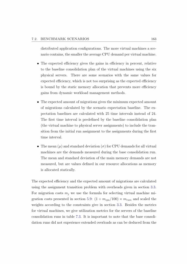
7.2. BENCHMARK SCENARIOS 163
distributed application configurations. The more virtual machines a sce-
nario contains, the smaller the average CPU demand per virtual machine.
• The expected efficiency gives the gains in efficiency in percent, relative
to the baseline consolidation plan of the virtual machines using the six
physical servers. There are some scenarios with the same values for
expected efficiency, which is not too surprising as the expected efficiency
is bound by the static memory allocation that prevents more efficiency
gains from dynamic workload management methods.
• The expected amount of migrations gives the minimum expected amount
of migrations calculated by the scenario expectation baseline. The ex-
pectation baselines are calculated with 25 time intervals instead of 24.
The first time interval is predefined by the baseline consolidation plan
(the virtual machine to physical server assignments) to include the tran-
sition from the initial run assignment to the assignments during the first
time interval.
• The mean (µ) and standard deviation (σ) for CPU demands for all virtual
machines are the demands measured during the base consolidation run.
The mean and standard deviation of the main memory demands are not
measured, but are values defined in our resource allocations as memory
is allocated statically.
The expected efficiency and the expected amount of migrations are calculated
using the assignment transition problem with overheads given in section 3.3.
For migration costs mj we use the formula for selecting virtual machine mi-
gration costs presented in section 5.9: (1 + mcpu/100) ×mram and scaled the
weights according to the constraints give in section 3.3. Besides the metrics
for virtual machines, we give utilization metrics for the servers of the baseline
consolidation runs in table 7.3. It is important to note that the base consoli-
dation runs did not experience extended overloads as can be deduced from the
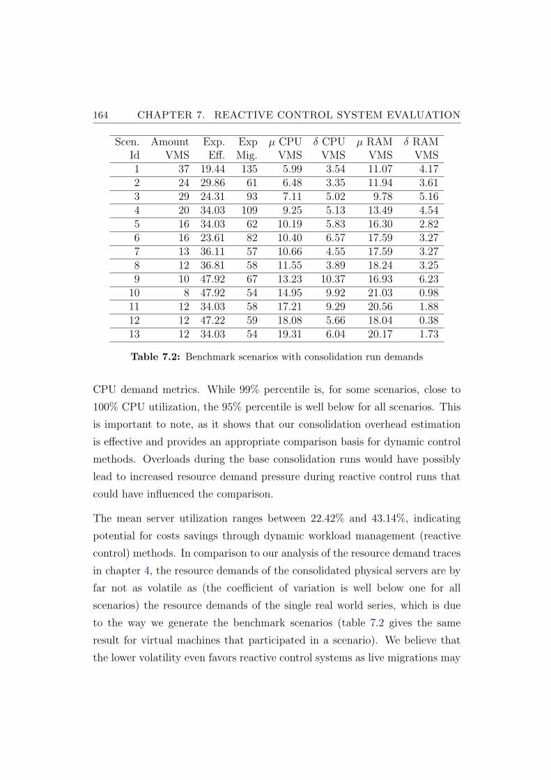
164 CHAPTER 7. REACTIVE CONTROL SYSTEM EVALUATION
Scen. Amount Exp. Exp µ CPU δ CPU µ RAM δ RAMId VMS Eff. Mig. VMS VMS VMS VMS1 37 19.44 135 5.99 3.54 11.07 4.172 24 29.86 61 6.48 3.35 11.94 3.613 29 24.31 93 7.11 5.02 9.78 5.164 20 34.03 109 9.25 5.13 13.49 4.545 16 34.03 62 10.19 5.83 16.30 2.826 16 23.61 82 10.40 6.57 17.59 3.277 13 36.11 57 10.66 4.55 17.59 3.278 12 36.81 58 11.55 3.89 18.24 3.259 10 47.92 67 13.23 10.37 16.93 6.23
10 8 47.92 54 14.95 9.92 21.03 0.9811 12 34.03 58 17.21 9.29 20.56 1.8812 12 47.22 59 18.08 5.66 18.04 0.3813 12 34.03 54 19.31 6.04 20.17 1.73
Table 7.2: Benchmark scenarios with consolidation run demands
CPU demand metrics. While 99% percentile is, for some scenarios, close to
100% CPU utilization, the 95% percentile is well below for all scenarios. This
is important to note, as it shows that our consolidation overhead estimation
is effective and provides an appropriate comparison basis for dynamic control
methods. Overloads during the base consolidation runs would have possibly
lead to increased resource demand pressure during reactive control runs that
could have influenced the comparison.
The mean server utilization ranges between 22.42% and 43.14%, indicating
potential for costs savings through dynamic workload management (reactive
control) methods. In comparison to our analysis of the resource demand traces
in chapter 4, the resource demands of the consolidated physical servers are by
far not as volatile as (the coefficient of variation is well below one for all
scenarios) the resource demands of the single real world series, which is due
to the way we generate the benchmark scenarios (table 7.2 gives the same
result for virtual machines that participated in a scenario). We believe that
the lower volatility even favors reactive control systems as live migrations may
7.2. BENCHMARK SCENARIOS 165
Scen. 25% 50% 75% 95% 99% µ σ GbyteId Server Server Server Server Server Server Server Sum1 16.86 40.85 66.76 91.20 99.38 43.14 28.48 171.802 16.04 29.08 40.81 65.35 76.95 30.02 18.11 150.513 6.86 25.78 60.10 87.87 94.41 34.59 29.64 120.854 5.37 21.20 53.88 85.13 95.24 31.21 28.78 125.945 4.86 19.54 49.15 74.74 89.36 27.97 25.61 124.916 4.41 25.03 51.41 82.15 98.13 30.75 27.38 128.177 4.49 18.54 40.94 62.28 93.84 24.42 22.13 105.908 6.0 23.62 40.49 67.32 85.10 26.19 21.44 114.449 4.92 19.84 39.32 72.30 84.63 25.62 23.46 107.69
10 4.12 17.08 34.01 64.92 79.01 22.42 20.88 106.2711 5.34 28.35 57.07 87.93 99.38 35.10 31.55 142.9412 12.25 33.86 62.16 84.21 96.20 39.09 29.27 162.3913 7.83 37.00 69.34 88.20 99.95 40.70 32.43 168.33
Table 7.3: Benchmark scenario consolidation runs, CPU andnetwork demands on physical servers
not be well suited for handling hard to predict, transient and sharp demand
spikes. Additionally, the mean utilization is about 2 to 3 times smaller than
the 99% percentile, which also indicates that the periods of high utilization
are rather short-lived. This observation supports the feasibility of resource
overbooking and more aggressive levels of consolidation that we will present in
section 7.6. We also give the aggregated network bandwidth consumed by the
clients for sending requests and receiving responses as well as the bandwidth for
communication between the application components (required by distributed
application configuration) during our consolidation runs. The numbers are
interesting as we will see that live migrations require a significant amount of
additional network bandwidth.
166 CHAPTER 7. REACTIVE CONTROL SYSTEM EVALUATION
7.2.1 Overall Statistics
In table 7.4 we give an overview of the metrics we elevated from the log data
collected during all experiment runs. We will see during the evaluation that
tuning reactive control system is a highwire act that has to balance reactivity
and control action overhead with application quality of service. Several factors
influence on the performance of reactive control that need to be in balance
to achieve high levels of operational efficiency. While it is rather simple to
implement a control system, its tuning is far from being easy, which is a main
reason why a study like ours does not exist up to now. To support our main
study goals we have chosen the following metrics.
1. µ Response time is the average response time of all operations of the
benchmark applications executed in a benchmark run.
2. σ Response time is the standard deviation of the response times of all
operations of the benchmark applications executing in a benchmark run.
3. 90% Response time is the 90% percentile of the response times of all
operations of the benchmark applications executed in a benchmark run.
The 90% percentile is used to set an acceptable level for quality of service
requirements. For our application this value is set to 2 seconds.
4. 99% Response time is the 99% percentile of the response times of all
operations of the benchmark applications executed in a benchmark run.
5. µ VM residence time is an indicator for system stability. It gives the
average time a virtual machine was executing on a physical server. The
longer the average resident time, the more stable we consider a system.
It is given in minutes.
6. µ Server down time is also an indicator for system stability. It gives the
average time a physical server was in an idle state, not executing any

7.2. BENCHMARK SCENARIOS 167
virtual machines. The longer the average down time, the more stable is
a system. It is given in minutes.
7. Realized efficiency gives the savings reactive control delivered in percent,
relative to the baseline consolidation run.
8. CPU overhead is the amount of additional CPU required for reactive
control. The overhead is due to the CPU demand for migrations on the
source and target server. However, consolidation overheads influence on
the measurements. The overhead is given in percent relative to the CPU
demands of the base consolidation run.
9. NET overhead is the amount of additional network bandwidth required
for reactive control. The overhead is due to the bandwidth demand for
migrations. The overhead is given in percent relative to the bandwidth
demands of the base consolidation run.
10. µ Migration duration specifies the mean duration of a migration in sec-
onds over all migrations in an experiment run.
11. Relative efficiency specifies the relative distance to the pre-computed
expected efficiency of a clairvoyant dynamic workload management
method. A negative values indicates a worse than expected efficiency,
a positive value indicates better than expected performance.
12. Relative amount migrations specifies the relative amount of migrations
triggered by the reactive control system in comparison to the pre-
computed minimum amount of expected migrations if resources are pro-
visioned as requested (including consolidation overhead estimation) by
a clairvoyant dynamic workload management method. Negative values
indicate that less migrations than the minimum amount of expected mi-
grations have been triggered and executed, positive values indicate that
more migrations were required.
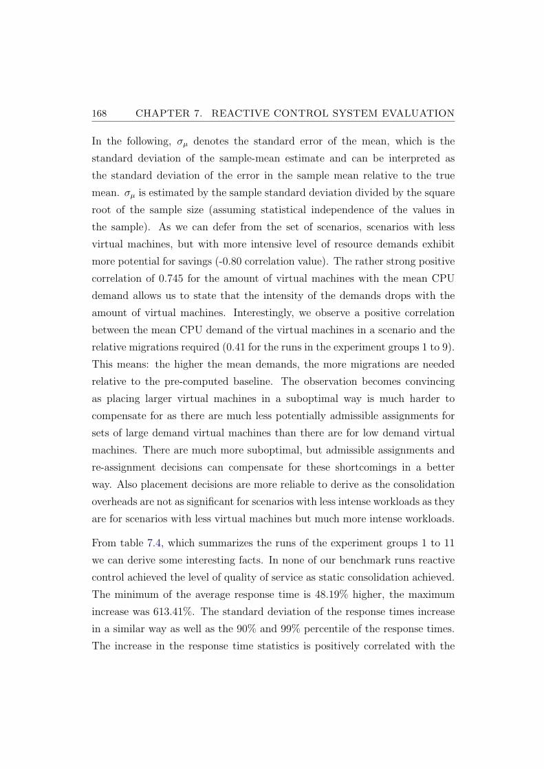
168 CHAPTER 7. REACTIVE CONTROL SYSTEM EVALUATION
In the following, σµ denotes the standard error of the mean, which is the
standard deviation of the sample-mean estimate and can be interpreted as
the standard deviation of the error in the sample mean relative to the true
mean. σµ is estimated by the sample standard deviation divided by the square
root of the sample size (assuming statistical independence of the values in
the sample). As we can defer from the set of scenarios, scenarios with less
virtual machines, but with more intensive level of resource demands exhibit
more potential for savings (-0.80 correlation value). The rather strong positive
correlation of 0.745 for the amount of virtual machines with the mean CPU
demand allows us to state that the intensity of the demands drops with the
amount of virtual machines. Interestingly, we observe a positive correlation
between the mean CPU demand of the virtual machines in a scenario and the
relative migrations required (0.41 for the runs in the experiment groups 1 to 9).
This means: the higher the mean demands, the more migrations are needed
relative to the pre-computed baseline. The observation becomes convincing
as placing larger virtual machines in a suboptimal way is much harder to
compensate for as there are much less potentially admissible assignments for
sets of large demand virtual machines than there are for low demand virtual
machines. There are much more suboptimal, but admissible assignments and
re-assignment decisions can compensate for these shortcomings in a better
way. Also placement decisions are more reliable to derive as the consolidation
overheads are not as significant for scenarios with less intense workloads as they
are for scenarios with less virtual machines but much more intense workloads.
From table 7.4, which summarizes the runs of the experiment groups 1 to 11
we can derive some interesting facts. In none of our benchmark runs reactive
control achieved the level of quality of service as static consolidation achieved.
The minimum of the average response time is 48.19% higher, the maximum
increase was 613.41%. The standard deviation of the response times increase
in a similar way as well as the 90% and 99% percentile of the response times.
The increase in the response time statistics is positively correlated with the
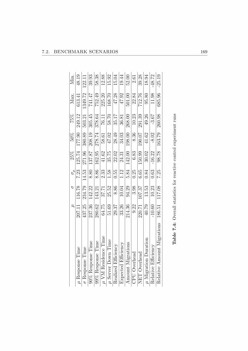
7.2. BENCHMARK SCENARIOS 169
µσ
σµ
25%
50%
75%
Max
.M
in.
µR
esp
onse
Tim
e20
7.11
116.
787.
2312
5.74
177.
9024
9.12
613.
4148
.19
σR
esp
onse
Tim
e43
7.25
234.
7914
.53
271.
9638
0.89
503.
2113
49.7
212
2.11
90%
Res
pon
seT
ime
237.
3614
2.22
8.80
137.
8720
8.19
305.
4574
1.47
39.9
399
%R
esp
onse
Tim
e28
0.62
143.
218.
8616
2.95
278.
7437
8.64
752.
4958
.38
µV
MR
esid
ence
Tim
e64
.75
37.7
12.
3341
.62
58.6
176
.11
225.
2012
.88
µSer
ver
Dow
nT
ime
51.6
925
.52
1.58
35.7
547
.02
58.7
016
8.70
15.9
2R
ealize
dE
ffici
ency
29.3
78.
860.
5522
.02
28.4
935
.17
47.2
815
.04
Exp
ecte
dE
ffici
ency
33.2
610
.04
1.12
24.3
134
.03
36.8
147
.92
19.4
4A
mou
nt
Mig
rati
ons
214.
3694
.29
5.84
142.
0019
8.00
268.
0050
1.00
52.0
0C
PU
Ove
rhea
d9.
223.
980.
256.
838.
3610
.23
22.8
42.
61N
ET
Ove
rhea
d22
0.71
107.
376.
6515
0.99
190.
0729
1.39
712.
7639
.28
µM
igra
tion
Dura
tion
40.7
913
.53
0.84
30.0
241
.62
49.2
695
.80
18.9
4R
elat
ive
Effi
cien
cy-1
0.60
10.2
30.
63-1
6.22
-8.0
2-3
.67
11.9
8-4
8.72
Rel
ativ
eA
mou
nt
Mig
rati
ons
186.
5111
7.08
7.25
98.7
816
3.79
260.
9868
5.96
-25.
19
Tab
le7.
4:O
vera
llst
atis
tics
for
reac
tive
cont
rol
expe
rim
ent
runs

170 CHAPTER 7. REACTIVE CONTROL SYSTEM EVALUATION
●
●●
●●●●●●●●●●●●●●
●●●
●●
●●●●
●●●●●
●
●
●●
●
●●●
●
●
●
●●●●●●●●●●
●●●
●
●●●
●
●
●
●●●
●●
●
●
●●
●
●
●●
●
●
●
●
●
●
●
●
●
●●
●●
●●●●
●●
●●
●●●●
●●●
●●●●
●
●
●●
●
●
●●
●
●
●
●
●
●
●
●
●
●
●
●
●
●
●
●
●
●
●
●
●●
●●●
●
●●
●●
●●●
●●●●
●●
●
●
●
●●●●●
●
●
●
●●●
●
●●
●
●
●
●
●●
●●●
●●
●●
●
●
●●
●●
●
●●
●
●●●
●
●
●●●●●
●
●●
●●
●
●
●●
●●●●●
●
●●●●●●●●●●●●
●●●●
●●●●●
●●●●●●●
●●
●●●●●●
●●●●
●●
6 8 10 12 14 16 18
100
200
300
400
500
600
Mean VM CPU Demand vs. Mean Rsp. Time Inc. (Cor.: 0.639 )
Mean VM CPU Demand
Mea
n R
sp. I
nc. (
%)
●●
●
●●●
●
●
●
●●●●●●●●
●●●●●
●●●●●●●●●●●●●
●
●
●
●
●
●
●●
●●●
●
●●
●●●
●●●●●●●●●●●
●●
●●
●
●
●●
●●
●●
●
●
●●
●●
●●
●●●
●●●●●●
●●
●●
●●●
●●
●●
●●●●
●
●
●●
●
●●●
●
●●
●●●
●
●
●
●
●
●
●
●●
●
●
●
●
●
●
●
●
●
●
●
●●●●●●
●●●●●
●●
●●●
●●●●●●
●●
●●
●
●
●
●●
●●●
●
●
●
●
●
●
●●
●
●
●
●●
●●
●
●
●
●
●●●
●●●●●
●●
●
●●
●●
●●●
●
●●
●
●●
●
●●●●●
●
●●●●●●●●●●●●
●●
●●
●
●●●●●●
●●●
●●●●
●
●
●●
●●
6 8 10 12 14 16 18
200
400
600
800
1200
Mean VM CPU Demand vs. Std. Deviation Rsp. Time Inc. (Cor.: 0.267 )
Mean VM CPU Demand
Std
. Dev
. Rsp
. Inc
. (%
)●●●
●
●●●
●●●●●●●●●●
●●●
●●
●●●●●
●
●
●
●
●●
●●
●
●
●●
●●
●●●●●
●●●
●●●●
●
●
●●●●
●●
●●●●
●●
●
●
●●
●
●
●●●
●
●●
●●
●●
●●●
●●
●●●●
●
●
●
●●●
●
●
●
●●●
●●●
●
●
●
●●
●
●●
●
●
●●
●
●
●●●
●●
●●
●●
●
●
●
●
●
●
●
●●
●
●
●●●●
●●●
●●●
●
●●
●●
●
●●●●
●
●
●●
●●●
●
●●●
●●
●
●
●●
●●
●
●
●●
●
●
●●
●●
●
●●
●
●●
●●●●●●●●
●
●
●
●●
●
●
●●
●●●●●●
●●●●●●●
●●●●●●●●●●●
●●●●●●●●●●
●●
●●
●●●●●●●●●●
6 8 10 12 14 16 18
100
300
500
700
Mean VM CPU Demand vs. 90th Percentile Rsp. Time Inc. (Cor.: 0.702 )
Mean VM CPU Demand
90th
Per
cent
ile R
sp. I
nc. (
%)
●
●●
●
●●
●●●
●●
●
●
●●●
●
●
●
●●
●
●●●●●
●
●
●
●●
●
●
●●
●
●
●
●
●
●
●
●●●
●●●●●●●●
●
●
●●●
●●
●
●●●
●●
●●
●
●
●
●
●●
●
●
●
●
●●
●●●
●
●
●
●●
●
●●
●
●
●●
●
●
●
●
●
●
●
●
●
●
●●
●
●
●●●
●●
●
●
●
●
●
●
●●
●
●●
●●
●
●
●
●
●●
●
●
●
●●
●
●
●●
●●●
●●●●●●●●
●
●
●
●●●●
●
●
●
●
●
●
●
●
●●●
●●
●
●●
●
●
●
●
●
●
●
●
●
●●
●●
●
●
●
●
●●●●
●
●●
●
●
●
●
●●
●●
●●
●
●
●●●●●●●●●●●●●●●●
●●
●●●●●●
●●●●●●●●●
●●●●●●●●●
●●
●●●●
6 8 10 12 14 16 18
100
300
500
700
Mean VM CPU Demand vs. 99th Percentile Rsp. Time Inc. (Cor.: 0.627 )
Mean VM CPU Demand
99th
Per
cent
ile R
sp. I
nc. (
%)
Figure 7.1: Mean CPU versus response times, experimentgroups 1 to 11
workload intensity (mean CPU demand per virtual machine) as shown in figure
7.1 for experiment groups 1 to 11, in figure 7.2 for experiment groups 1 to 7 and
in figure 7.3 for experiment groups 1 to 2. On average, reactive control comes
close to the baseline efficiency. The average of −10.60% for relative efficiency,
meaning the expected efficiency was not achieved, indicates an absolute loss
in operational efficiency of about 4%. The difference is significant: we tested
the null hypotheses that the true mean is zero (%) using a one-sample, two-
tailed Wilcoxon signed rank test as the distribution of the relative efficiency
values is non-normal as shown the quantile-quantile plot in figure 7.4, even
after filtering the tails. The obtained p-value of < 2.2e−16 leads us to the re-
jection of the null-hypthesis. The 95 % confidence interval is −11.84,−9.35%.
This indicates to us that while reactive control is able to deliver even better
performance than the expectation baseline, the minimum efficiency is 11.98%,
that is some runs achieved better efficiency than the expected efficiency, given
the right control parameter configuration for a scenario. The quantile-quantile
plot in figure 7.4 and the distribution of the relative efficiencies of the runs of
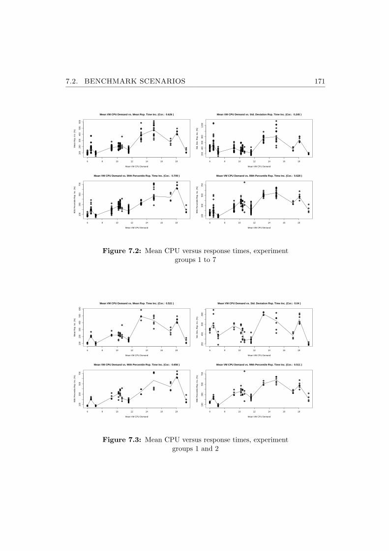
7.2. BENCHMARK SCENARIOS 171
●
●●
●●●●●●●●●●●●●●
●●
●●●●
●
●
●●
●●●●●●●●●
●●●
●
●●●
●
●
●
●
●
●
●
●●
●
●
●
●
●
●
●
●
●
●●
●●
●●●
●●●●
●
●
●●
●
●
●
●
●
●
●
●
●
●
●
●
●
●
●
●
●
●
●
●
●●
●●●
●
●●
●●
●●●
●●●●
●●
●
●
●
●
●
●●●
●
●●
●
●
●
●
●●
●●
●
●●
●
●●
●
●●●
●
●
●●●●●
●
●●
●●●●●
●
●●●●●●●●
●●●●
●●●●●
●
●●
●●
●●●●
●●
6 8 10 12 14 16 18
100
200
300
400
500
600
Mean VM CPU Demand vs. Mean Rsp. Time Inc. (Cor.: 0.626 )
Mean VM CPU Demand
Mea
n R
sp. I
nc. (
%)
●●
●
●●●
●
●
●
●●●●●●●●
●●
●●●●●●●●
●●●
●
●●
●●●
●●●●●●●●●●
●
●
●●
●●
●
●
●●
●●
●●
●●●
●
●●
●●
●●●●
●
●
●●
●
●●
●●●
●
●
●
●
●
●
●
●●
●
●
●
●
●
●
●
●
●
●
●
●●●●●●
●●●●●
●●
●●●
●●
●●
●
●
●
●●
●●●
●
●●
●
●
●●
●
●
●
●
●●●
●●●●●
●●
●
●●
●●
●
●●
●
●●●●●
●
●●●●●●●●
●●
●●
●
●●●●
●
●●
●●
6 8 10 12 14 16 18
200
400
600
800
1200
Mean VM CPU Demand vs. Std. Deviation Rsp. Time Inc. (Cor.: 0.245 )
Mean VM CPU Demand
Std
. Dev
. Rsp
. Inc
. (%
)
●●●
●
●●●
●●●●●●●●●●
●●
●
●
●
●
●●
●●
●●●
●●●
●●●●
●
●
●●●●
●●
●
●
●
●
●
●●●
●
●●
●●
●●
●●●
●
●
●
●●●
●●●
●
●
●
●
●
●
●●
●
●
●●●
●●
●●
●●
●
●
●
●
●
●
●
●●
●
●
●●●●
●●●
●●●
●
●●
●●
●
●●
●●●
●
●●●
●●
●●
●
●●
●
●●
●
●●
●
●●
●●●●●●●●
●
●
●
●●●●●●
●●●●●●●●●●●●●●
●●●●
●●
●●●●●●●●
6 8 10 12 14 16 18
100
300
500
700
Mean VM CPU Demand vs. 90th Percentile Rsp. Time Inc. (Cor.: 0.709 )
Mean VM CPU Demand
90th
Per
cent
ile R
sp. I
nc. (
%)
●
●●
●
●●
●●●
●●
●
●
●●●
●
●
●
●
●
●
●●
●
●
●
●●●
●●●●●●●●
●
●
●●●
●●
●
●●
●
●
●●
●
●
●
●
●●
●●●
●
●
●
●
●
●
●
●
●
●
●●
●
●
●
●
●
●
●
●
●
●●
●
●●
●●
●
●
●
●
●●
●
●
●
●●
●
●
●●
●●●
●●●●●●●●
●
●
●
●
●
●
●
●
●
●●●
●●
●
●
●
●
●
●
●●
●
●
●
●
●●●●
●
●●
●
●
●
●
●●
●●
●●●●●●●●●●
●●
●●●●●●
●●●●●●●●
●●
●●●●
6 8 10 12 14 16 18
100
300
500
700
Mean VM CPU Demand vs. 99th Percentile Rsp. Time Inc. (Cor.: 0.628 )
Mean VM CPU Demand
99th
Per
cent
ile R
sp. I
nc. (
%)
Figure 7.2: Mean CPU versus response times, experimentgroups 1 to 7
●
●●
●
●●●●
●●●●●●
●
●
●●
●
●
●
●
●
●
●
●
●
●●
●●
●
●
●
●
●
●
●
●
●
●
●
●
●
●●●
●
●
●
●
●
●●
●
●●
●●●●●
●●●●●
6 8 10 12 14 16 18
100
200
300
400
500
600
Mean VM CPU Demand vs. Mean Rsp. Time Inc. (Cor.: 0.521 )
Mean VM CPU Demand
Mea
n R
sp. I
nc. (
%)
●
●
●
●
●
●
●
●
●●●
●
●
●
●●
●●
●
●
●
●
●●
●●
●●●
●
●●
●
●
●
●
●●
●
●
●
●
●
●●
●
●
●
●
●●
●
●
●
●
●
●
●●
●
●
●
●
●
●
●
●
6 8 10 12 14 16 18
200
400
600
800
Mean VM CPU Demand vs. Std. Deviation Rsp. Time Inc. (Cor.: 0.04 )
Mean VM CPU Demand
Std
. Dev
. Rsp
. Inc
. (%
)
●●●
●
●●●
●
●●●
●●●
●
●
●●●
●
●●
●●
●●
●●●
●
●
●
●
●
●●
●
●
●●●
●●
●
●●
●
●●
●●
●
●●
●
●●
●●●●●●●●
●●
6 8 10 12 14 16 18
100
300
500
700
Mean VM CPU Demand vs. 90th Percentile Rsp. Time Inc. (Cor.: 0.656 )
Mean VM CPU Demand
90th
Per
cent
ile R
sp. I
nc. (
%)
●
●●
●
●●
●●
●●●
●●●
●
●
●●
●
●
●
●
●●
●●●
●
●
●
●
●
●
●
●
●
●
●
●●
●
●●
●
●●
●
●
●
●●
●
●
●
●
●●
●●
●●●●
●●●●
6 8 10 12 14 16 18
100
300
500
700
Mean VM CPU Demand vs. 99th Percentile Rsp. Time Inc. (Cor.: 0.511 )
Mean VM CPU Demand
99th
Per
cent
ile R
sp. I
nc. (
%)
Figure 7.3: Mean CPU versus response times, experimentgroups 1 and 2

172 CHAPTER 7. REACTIVE CONTROL SYSTEM EVALUATION
●
●
●●
●●
●●●
●
●
●
●
●
●
●
●
●●
●
●
●
●
●
●●
●
●
●●
●●
●●
●
●
●●
●●
●
●
●
●
●
●
●
●
●
●●
●
●
●
●
●
●●
●
●●●
●
●
●
●
●
●
●
●
●
●
●
●
●
●
●
●
●
●
●●
●
●
●
●
●
●
●
●
●
●
●●
●
●
●
●
●
●
●
●●
●
●
●●
●
●●
●
●
●
●
●
●
●
●
●
●
●
●
●●
●
●●
●●
●
●
●
●
●
●●●
●
●
●
●
●
●
●
●
● ●
●
●
●
●
●
●●
●●
●
●
●●
●●
●
●●
●●●
●
●
●
●
●●
●
●
●●
●
●
●●
●
●
●
●●●
●
●
●
●
●
●
●
●
●
●
●
●●●
●●
●
●
●
●
●●
●
●
●
●
●
●
●
●●
●
●
●
●
●
●
●
●
●
●
●
●
●
●
●
●●●
●
●
●
●
●
●
●
●
●
●
●
●
●●
●
●
●●
●
●
●
●●
●
−3 −2 −1 0 1 2 3
−50
−40
−30
−20
−10
010
Relative Efficiency, All Experiments, QQ−Plot
Mean Efficiency: −10.596 %Theoretical Quantiles
Rel
ativ
e E
ffici
ency
Distribution of Relative Efficiency, All Experiments
Relative Efficiency (%)
Den
sity
−50 −40 −30 −20 −10 0 10
0.00
0.01
0.02
0.03
0.04
0.05
Figure 7.4: Distribution of relative efficiency, all experiment runs
−40 −20 0 20
0.00
0.02
0.04
0.06
0.08
0.10
Relative Efficiency Density Estimates
Relative Efficiency (%)
Den
sity
Scenarios 1 − 6, 8−10Scenarios 1,2,3,4,5,8,9Scenario 6Scenario 10
Figure 7.5: Distribution of relative efficiency, selected scenarios
the experiment groups 1 - 11 indicate that the population mean is influenced
by the large left tail, reaching out to almost 50% of efficiency losses. The left
tail can be explained by considerable differences in the achieved level of relative
efficiency for some scenarios. As can be deferred from table 7.11, two scenarios
(6 and 10) expose much lower efficiency in contrast to the remaining scenarios.
In figure 7.5 and table 7.6, which gives detailed summary statistics, we provide
more details on the relative efficiency distribution of the two scenarios as well
as on the distribution of all scenarios and all remaining scenarios. The dif-
ferences are attributed to the main memory demands of the virtual machines
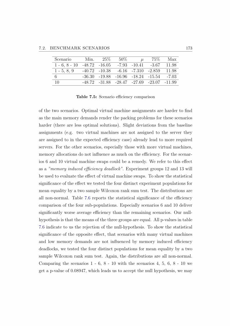
7.2. BENCHMARK SCENARIOS 173
Scenario Min. 25% 50% µ 75% Max1 - 6, 8 - 10 -48.72 -16.05 -7.93 -10.41 -3.67 11.981 - 5, 8, 9 -40.72 -10.38 -6.16 -7.310 -2.859 11.986 -36.30 -19.88 -16.96 -18.24 -15.54 -7.0310 -48.72 -31.88 -28.47 -27.69 -23.07 -11.99
Table 7.5: Scenario efficiency comparison
of the two scenarios. Optimal virtual machine assignments are harder to find
as the main memory demands render the packing problems for these scenarios
harder (there are less optimal solutions). Slight deviations from the baseline
assignments (e.g. two virtual machines are not assigned to the server they
are assigned to in the expected efficiency case) already lead to more required
servers. For the other scenarios, especially those with more virtual machines,
memory allocations do not influence as much on the efficiency. For the scenar-
ios 6 and 10 virtual machine swaps could be a remedy. We refer to this effect
as a ”memory induced efficiency deadlock”. Experiment groups 12 and 13 will
be used to evaluate the effect of virtual machine swaps. To show the statistical
significance of the effect we tested the four distinct experiment populations for
mean equality by a two sample Wilcoxon rank sum test. The distributions are
all non-normal. Table 7.6 reports the statistical significance of the efficiency
comparison of the four sub-populations. Especially scenarios 6 and 10 deliver
significantly worse average efficiency than the remaining scenarios. Our null-
hypothesis is that the means of the three groups are equal. All p-values in table
7.6 indicate to us the rejection of the null-hypothesis. To show the statistical
significance of the opposite effect, that scenarios with many virtual machines
and low memory demands are not influenced by memory induced efficiency
deadlocks, we tested the four distinct populations for mean equality by a two
sample Wilcoxon rank sum test. Again, the distributions are all non-normal.
Comparing the scenarios 1 - 6, 8 - 10 with the scenarios 4, 5, 6, 8 - 10 we
get a p-value of 0.08947, which leads us to accept the null hypothesis, we may
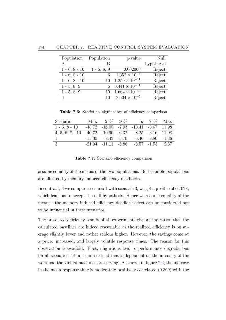
174 CHAPTER 7. REACTIVE CONTROL SYSTEM EVALUATION
Population Population p-value NullA B hypothesis1 - 6, 8 - 10 1 - 5, 8, 9 0.002006 Reject1 - 6, 8 - 10 6 1.352× 10⁻⁶ Reject1 - 6, 8 - 10 10 1.259× 10⁻¹¹ Reject1 - 5, 8, 9 6 3.441× 10⁻¹¹ Reject1 - 5, 8, 9 10 1.664× 10⁻¹⁴ Reject6 10 2.504× 10⁻⁵ Reject
Table 7.6: Statistical significance of efficiency comparison
Scenario Min. 25% 50% µ 75% Max1 - 6, 8 - 10 -48.72 -16.05 -7.93 -10.41 -3.67 11.984, 5, 6, 8 - 10 -40.72 -10.90 -6.32 -8.25 -3.16 11.981 -15.30 -8.43 -5.70 -6.46 -3.80 -1.363 -21.04 -11.11 -5.86 -6.57 -1.53 2.37
Table 7.7: Scenario efficiency comparison
assume equality of the means of the two populations. Both sample populations
are affected by memory induced efficiency deadlocks.
In contrast, if we compare scenario 1 with scenario 3, we get a p-value of 0.7028,
which leads us to accept the null hypothesis. Hence we assume equality of the
means - the memory induced efficiency deadlock effect can be considered not
to be influential in these scenarios.
The presented efficiency results of all experiments give an indication that the
calculated baselines are indeed reasonable as the realized efficiency is on av-
erage slightly lower and rather seldom higher. However, the savings come at
a price: increased, and largely volatile response times. The reason for this
observation is two-fold. First, migrations lead to performance degradations
for all scenarios. To a certain extend that is dependent on the intensity of the
workload the virtual machines are serving. As shown in figure 7.6, the increase
in the mean response time is moderately positively correlated (0.369) with the
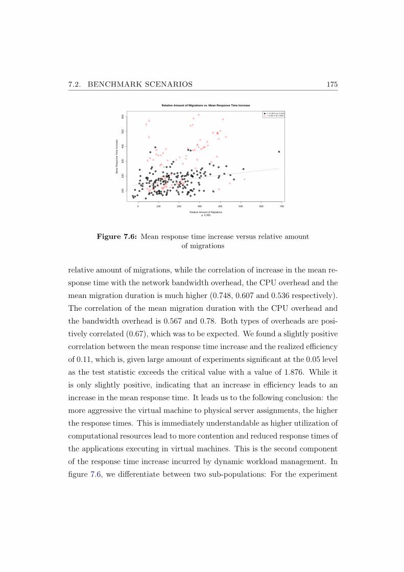
7.2. BENCHMARK SCENARIOS 175
●
● ●●
●
●
●●●
●●
●●
●
●
● ●●
●
●
●
●●●
●
●
●
●
●
●
●
●
●
●
●
●
●
●●
●
● ●
●
●
●
●●
●
● ●
●
●
●
●
●●
●
●
●
●
●
●
●
●
●
●
●●
●
●
●●
●●
●
●●
●
●
●
●
●●
●
●
●
●
●
●●
●
●
●
●
●
●
●
●
●●
●
●●
●
●●
●
●
●
●
● ●
●
●
●
● ●
●●
●
●
●
●
●●
●
●
●
●
●
●
●● ●
●
●
●●●
●●
●●
●
●
●
●●
●●●●
● ●●
●
●
●
●
●
●
●●
●●
●
●
●●
●●
0 100 200 300 400 500 600 700
100
200
300
400
500
600
Relative Amount of Migrations vs. Mean Response Time Increase
ρ: 0.369Relative Amount of Migrations
Mea
n R
espo
nse
Tim
e In
crea
se● <= 11.88 % (ρ: 0.424)
> 11.88 % (ρ: 0.556)
Figure 7.6: Mean response time increase versus relative amountof migrations
relative amount of migrations, while the correlation of increase in the mean re-
sponse time with the network bandwidth overhead, the CPU overhead and the
mean migration duration is much higher (0.748, 0.607 and 0.536 respectively).
The correlation of the mean migration duration with the CPU overhead and
the bandwidth overhead is 0.567 and 0.78. Both types of overheads are posi-
tively correlated (0.67), which was to be expected. We found a slightly positive
correlation between the mean response time increase and the realized efficiency
of 0.11, which is, given large amount of experiments significant at the 0.05 level
as the test statistic exceeds the critical value with a value of 1.876. While it
is only slightly positive, indicating that an increase in efficiency leads to an
increase in the mean response time. It leads us to the following conclusion: the
more aggressive the virtual machine to physical server assignments, the higher
the response times. This is immediately understandable as higher utilization of
computational resources lead to more contention and reduced response times of
the applications executing in virtual machines. This is the second component
of the response time increase incurred by dynamic workload management. In
figure 7.6, we differentiate between two sub-populations: For the experiment
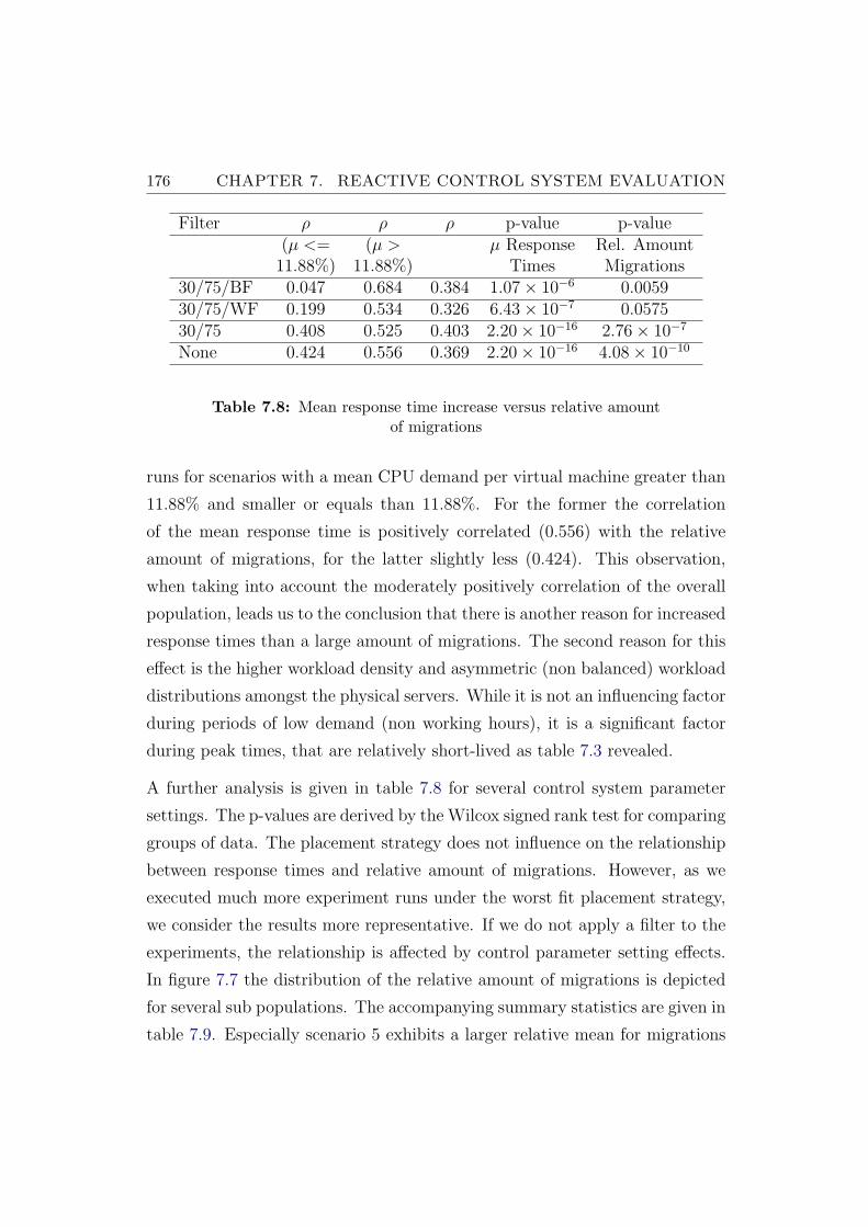
176 CHAPTER 7. REACTIVE CONTROL SYSTEM EVALUATION
Filter ρ ρ ρ p-value p-value(µ <= (µ > µ Response Rel. Amount
11.88%) 11.88%) Times Migrations30/75/BF 0.047 0.684 0.384 1.07× 10⁻⁶ 0.005930/75/WF 0.199 0.534 0.326 6.43× 10⁻⁷ 0.057530/75 0.408 0.525 0.403 2.20× 10⁻¹⁶ 2.76× 10⁻⁷
None 0.424 0.556 0.369 2.20× 10⁻¹⁶ 4.08× 10⁻¹⁰
Table 7.8: Mean response time increase versus relative amountof migrations
runs for scenarios with a mean CPU demand per virtual machine greater than
11.88% and smaller or equals than 11.88%. For the former the correlation
of the mean response time is positively correlated (0.556) with the relative
amount of migrations, for the latter slightly less (0.424). This observation,
when taking into account the moderately positively correlation of the overall
population, leads us to the conclusion that there is another reason for increased
response times than a large amount of migrations. The second reason for this
effect is the higher workload density and asymmetric (non balanced) workload
distributions amongst the physical servers. While it is not an influencing factor
during periods of low demand (non working hours), it is a significant factor
during peak times, that are relatively short-lived as table 7.3 revealed.
A further analysis is given in table 7.8 for several control system parameter
settings. The p-values are derived by the Wilcox signed rank test for comparing
groups of data. The placement strategy does not influence on the relationship
between response times and relative amount of migrations. However, as we
executed much more experiment runs under the worst fit placement strategy,
we consider the results more representative. If we do not apply a filter to the
experiments, the relationship is affected by control parameter setting effects.
In figure 7.7 the distribution of the relative amount of migrations is depicted
for several sub populations. The accompanying summary statistics are given in
table 7.9. Especially scenario 5 exhibits a larger relative mean for migrations
7.2. BENCHMARK SCENARIOS 177
−100 0 100 200 300 400 500 600
0.00
00.
001
0.00
20.
003
0.00
40.
005
Relative Migrations Density Estimates
Relative Migrations (%)
Den
sity
Scenarios 1−6,8−10Scenarios 1−4,6,8Scenario 5
Figure 7.7: Relative amount of migrations
Scenario Min. 25% 50% µ 75% Max1 - 6, 8 - 10 -25.19 92.79 150.00 172.90 243.50 512.901 - 4, 6, 8 -10 -25.19 80.68 134.20 151.20 216.30 449.205 59.68 139.90 216.90 219.30 296.00 512.90
Table 7.9: Scenario migration comparison
than all other scenarios. However no statistical significance can be observed
by comparing the three sub-populations using a Wilcoxon rank sum test. The
obtained p-values range between 0.0435 (comparing 1 - 6, 8 - 10 and 1 - 4, 6, 8
-10 ), 0.01453 (comparing 1 - 6, 8 - 10 and 5) and 0.0004525 (comparing 1 - 4,
6, 8 -10 and 5). These values do not allow us to reject the null hypothesis of
equal means. As we can also give no rational for the result, we believe that the
difference is obtained by chance rather than a systematic deviation induced
by scenario specifics. Analyzing the relative amount of migrations we notice
that on average 186.51% more migrations were required than calculated by he
expectation baseline. However, we also executed experiment runs that required
substantially less migrations, as the minimum is 25.19% less migrations than
the expectation baseline. Especially high values for detection delays lead to
this observation. If the detection delay is set too high, transient overloads or
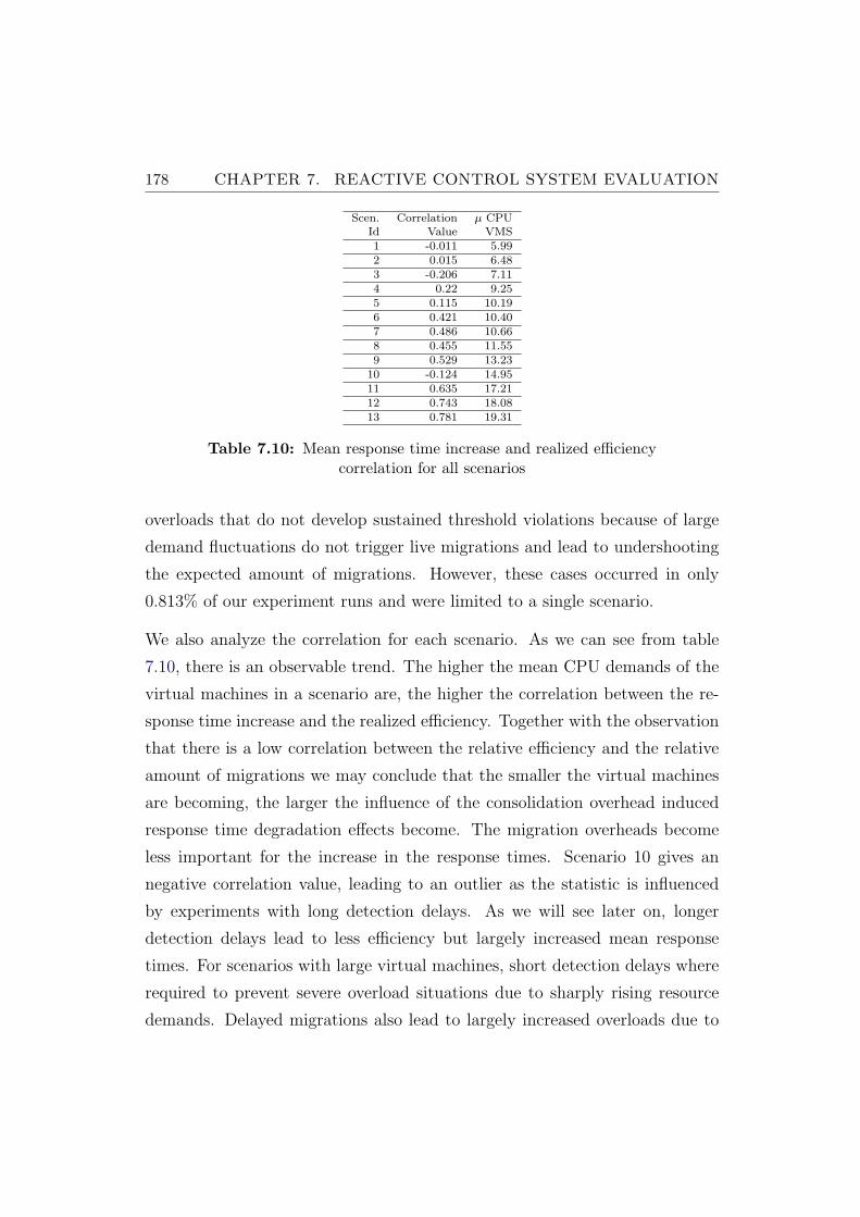
178 CHAPTER 7. REACTIVE CONTROL SYSTEM EVALUATION
Scen. Correlation µ CPUId Value VMS1 -0.011 5.992 0.015 6.483 -0.206 7.114 0.22 9.255 0.115 10.196 0.421 10.407 0.486 10.668 0.455 11.559 0.529 13.23
10 -0.124 14.9511 0.635 17.2112 0.743 18.0813 0.781 19.31
Table 7.10: Mean response time increase and realized efficiencycorrelation for all scenarios
overloads that do not develop sustained threshold violations because of large
demand fluctuations do not trigger live migrations and lead to undershooting
the expected amount of migrations. However, these cases occurred in only
0.813% of our experiment runs and were limited to a single scenario.
We also analyze the correlation for each scenario. As we can see from table
7.10, there is an observable trend. The higher the mean CPU demands of the
virtual machines in a scenario are, the higher the correlation between the re-
sponse time increase and the realized efficiency. Together with the observation
that there is a low correlation between the relative efficiency and the relative
amount of migrations we may conclude that the smaller the virtual machines
are becoming, the larger the influence of the consolidation overhead induced
response time degradation effects become. The migration overheads become
less important for the increase in the response times. Scenario 10 gives an
negative correlation value, leading to an outlier as the statistic is influenced
by experiments with long detection delays. As we will see later on, longer
detection delays lead to less efficiency but largely increased mean response
times. For scenarios with large virtual machines, short detection delays where
required to prevent severe overload situations due to sharply rising resource
demands. Delayed migrations also lead to largely increased overloads due to
7.2. BENCHMARK SCENARIOS 179
high migration overheads. The runs with 85% upper thresholds lead to im-
proved efficiency but largely increased response times because the higher upper
threshold often lead to severe overload situations. However, we removed these
experiments for the correlation calculation. The two tables 7.11 and 7.12 give
summary statistics for each scenario. We may observe that the three metrics,
average migration time, CPU overhead and bandwidth overhead in combina-
tion are a measurement for the potential impact a migration has on application
performance: the more time it takes and the more overhead it generates, the
more a migration impacts on application performance. The correlation with
CPU overhead is not as distinctive as the correlation with bandwidth over-
head, which is due to the fact that the measured CPU overhead is influenced
by the consolidation overheads: Different combinations of virtual machines,
with different demand levels cause different levels of CPU utilization. The
bandwidth overhead is consequently a better indicator for workload intensity
and performance impact.
Also, a large amount of migrations is not a guarantee for efficiency: the relative
efficiency is only slightly positively correlated (0.0363) with the relative amount
of migrations. Our claim that system stability is something to aim at, is
supported by the negative correlation of -0.4587607 between the mean response
time increase and the mean virtual machine residence time. We use the two
metrics, mean server down time and mean virtual machine residence time
to characterize a systems stability. One would expect that the two are almost
perfectly correlated. However a correlation factor of 0.675 gives rise to assume a
weaker relationship and indicates that large amounts of migrations and control
system reactivity do not necessarily lead to energy savings. The increase in
the mean response time is moderately negatively correlated (-0.459) with the
mean residence time, the relative amount of migrations is stronger correlated
with the mean residence time (-0.686).
Reactive control initiates virtual machines migrations during times of peak
demands to prevent overloads rather than to turn down servers. However,
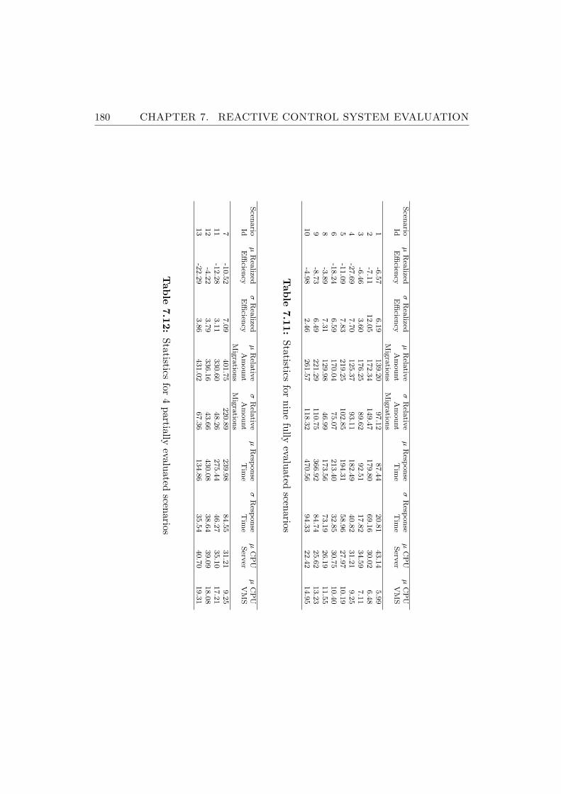
180 CHAPTER 7. REACTIVE CONTROL SYSTEM EVALUATION
Scen
ario
µR
ealized
σR
ealized
µR
elativ
eσ
Rela
tive
µR
espon
seσ
Resp
on
seµ
CP
Uµ
CP
UId
Effi
ciency
Effi
ciency
Am
ou
nt
Am
ou
nt
Tim
eT
ime
Serv
erV
MS
Mig
ratio
ns
Mig
ratio
ns
1-6
.57
6.1
9139.2
097.1
287.4
420.8
143.1
45.9
92
-7.1
112.0
5172.3
4149.4
7179.8
069.1
630.0
26.4
83
-6.4
63.6
0176.2
589.6
292.5
117.8
234.5
97.1
14
-27.6
97.7
0125.3
793.1
1182.4
940.8
231.2
19.2
55
-11.0
97.8
3219.2
5102.8
5194.3
158.9
627.9
710.1
96
-18.2
46.5
9170.0
475.0
7213.4
032.8
530.7
510.4
08
-3.8
97.3
1129.9
846.9
9173.5
673.1
926.1
911.5
59
-8.7
36.4
9221.2
9110.7
5366.9
284.7
425.6
213.2
310
-4.9
82.4
6261.5
7118.3
2470.5
694.3
322.4
214.9
5
Tab
le7.11:
Statisticsfor
ninefully
evaluatedscenarios
Scen
ario
µR
ealized
σR
ealized
µR
elativ
eσ
Rela
tive
µR
espon
seσ
Resp
on
seµ
CP
Uµ
CP
UId
Effi
ciency
Effi
ciency
Am
ou
nt
Am
ou
nt
Tim
eT
ime
Serv
erV
MS
Mig
ratio
ns
Mig
ratio
ns
7-1
0.5
27.0
9401.7
5220.8
9239.9
884.5
531.2
19.2
511
-12.2
83.1
1330.6
048.2
6275.4
446.2
735.1
017.2
112
-4.2
23.7
9336.1
643.6
6430.0
838.6
439.0
918.0
813
-22.2
93.8
6431.0
267.3
6134.8
635.5
440.7
019.3
1
Tab
le7.12:
Statisticsfor
4partially
evaluatedscenarios
7.2. BENCHMARK SCENARIOS 181
during peak times placement decisions become much more risk affected as
projected resource demands become much more inaccurate, leading to system
oscillations.
7.2.2 Placement Strategy: Worst Fit versus Best Fit
We used two virtual machine placement decisions in our experiments, namely
the worst-fit (WF) and best-fit (BF) placement rules. In case a migration
is triggered, WF selects as the target server the one that has the most free
capacity after the virtual machine is migrated, the BF rule places the virtual
machine on the server with the least capacity available after the migration.
We expected the more aggressive BF strategy to perform better in terms of
realized efficiency. As we use the t-test in the following to account for statistical
significance, we test all data samples using the Anderson-Darling and Shapiro-
Wilk test. The two tests reject the hypothesis of normality when the calculated
p-value is ≤ 0.05. Failing the normality tests allows us to state that with 95%
confidence, the data does not fit the normal distribution. However, passing the
normality test allows us to state no significant departure from normality was
found. This is a sufficient precondition to employ the t-test. We use the two
tests, as it is well known that the Anderson-Darling is often found to lead to
problematic results when applied to real world data containing ties. To ensure
the correctness of the statistical test procedures we hence employed a second
test, namely the Shapiro-Wilk test to underpin our findings.
7.2.2.1 Low Detection Delay
The following comparison is based on all experiments (experiment groups 1 -
11) with detection delay 1, and 30/75 thresholds. We present the results of our
comparison in table 7.13. We show the differences in percent, with BF being
the point of reference. A negative value means worse, a positive better then
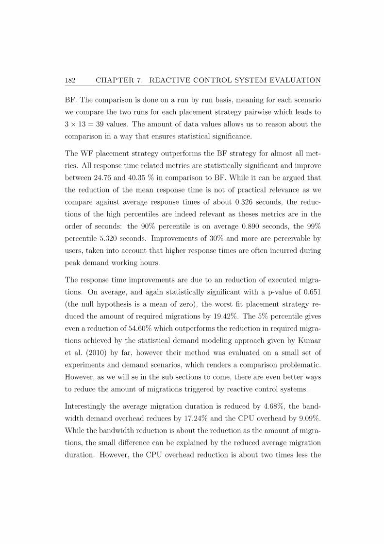
182 CHAPTER 7. REACTIVE CONTROL SYSTEM EVALUATION
BF. The comparison is done on a run by run basis, meaning for each scenario
we compare the two runs for each placement strategy pairwise which leads to
3× 13 = 39 values. The amount of data values allows us to reason about the
comparison in a way that ensures statistical significance.
The WF placement strategy outperforms the BF strategy for almost all met-
rics. All response time related metrics are statistically significant and improve
between 24.76 and 40.35 % in comparison to BF. While it can be argued that
the reduction of the mean response time is not of practical relevance as we
compare against average response times of about 0.326 seconds, the reduc-
tions of the high percentiles are indeed relevant as theses metrics are in the
order of seconds: the 90% percentile is on average 0.890 seconds, the 99%
percentile 5.320 seconds. Improvements of 30% and more are perceivable by
users, taken into account that higher response times are often incurred during
peak demand working hours.
The response time improvements are due to an reduction of executed migra-
tions. On average, and again statistically significant with a p-value of 0.651
(the null hypothesis is a mean of zero), the worst fit placement strategy re-
duced the amount of required migrations by 19.42%. The 5% percentile gives
even a reduction of 54.60% which outperforms the reduction in required migra-
tions achieved by the statistical demand modeling approach given by Kumar
et al. (2010) by far, however their method was evaluated on a small set of
experiments and demand scenarios, which renders a comparison problematic.
However, as we will se in the sub sections to come, there are even better ways
to reduce the amount of migrations triggered by reactive control systems.
Interestingly the average migration duration is reduced by 4.68%, the band-
width demand overhead reduces by 17.24% and the CPU overhead by 9.09%.
While the bandwidth reduction is about the reduction as the amount of migra-
tions, the small difference can be explained by the reduced average migration
duration. However, the CPU overhead reduction is about two times less the
7.2. BENCHMARK SCENARIOS 183
Metric 5% 50% µ 95% σRelative Amount Migrations -54.60 -14.81 -19.42 2.64 24.34µ Response Time -65.91 -21.32 -24.76 3.52 22.08σ Response Time -101.91 -34.12 -40.35 4.82 35.4190% Response Time -85.10 -27.54 -30.26 11.09 30.1899% Response Time -68.79 -23.36 -26.15 6.16 26.24Realized Efficiency -9.10 0.00 -0.10 11.60 6.03µ VM Residence Time -13.43 11.91 13.98 54.76 19.23µ Server Down Time -50.82 8.69 5.07 63.73 41.65CPU Overhead -87.11 2.74 -9.09 18.57 37.77NET Overhead -58.44 -8.81 -17.24 4.74 30.67µ Migration Duration -23.91 0.18 -4.68 11.58 22.52
Table 7.13: Worst-fit versus best-fit, low delay comparison
reductions of the migrations. This is an effect of the varying consolidation
overheads and the reduced time required for the migrations. We have to note
that the reduction of the migration duration is statistically not significant, but
occurred by chance. The Anderson-Darling test for normality gave a p-value
= 0.724, the Shapiro-Wilk of 0.492. Hence the assumption of normality can be
supported. We carried out a two sided, one-sample t-test testing with the null
hypothesis that the mean is zero. A p-value of 0.682 lead us to accept the null
hypothesis. We also calculate the correlation factors for the data that were
used in this comparison for validating the results with the results obtained on
the overall data (experiment groups 1 - 11). We found that the correlation be-
tween the relative amount of migrations and the mean response times increase
on the subset is 0.399, compared to 0.74 on the overall data set. The reduction
was to be expected as the highly reactive setup with a detection delay of one
leads to an excessive amount of migrations and the reductions obtained by the
WF placement strategy are only one way to reduce the amount of migrations,
as we will see later on.
Most important, we could not observe a significant reduction in operational
184 CHAPTER 7. REACTIVE CONTROL SYSTEM EVALUATION
efficiency for the WF placement strategy. First, the Anderson Darling and
Shapiro-Wilk test resulted in p-values of 0.3244 and 0.1335. The low p-values
where caused by outliers: when we filtered out the values above and below
the 95% percentile and 5% percentile the test resulted in p-values of 0.809
and 0.531. The two-sided t-test resulted in p-values of 0.5441 and 0.8763
respectively that allowed us to accept the null hypothesis of the mean being
equal to zero, the 95% confidence interval is given by {−1.37, 1.17}.
7.2.2.2 Optimal Detection Delay
The following comparison is based on the experiments (experiment groups
5 - 9) with the optimal detection delay with respect to the mean increase in
response time, and 30/75 thresholds. We present the results of our comparison
in table 7.14. We show the differences in percent, again BF being the point
of reference, that is a negative value means less, a positive more then BF.
The comparison is done on a run by run basis, meaning for each scenario we
compare the two runs for each placement strategy pairwise which leads to 3×11 = 33 values. The WF placement strategy still outperforms the BF strategy
for almost all metrics. All response time related are statistically significant and
improve between 31.75 and 39.56%. While it can be argued that the reduction
of the mean response time is not impressive as we compare against average
response times of about 0.326 seconds, the reductions in the high percentiles
are indeed relevant as theses metrics are in the order of seconds: the 90%
percentile is on average 0.780 seconds, the 99% percentile 6.010 seconds.
The response time improvements are again mainly due to a reduction of ex-
ecuted migrations, however compared to the low detection delay comparison
the mean reduction was lower. A two sample t-test lead to a p-value of 0.0206
when comparing the means of the two samples under the null hypothesis that
the two means are equal. The low p-value requires us to reject the null hypoth-
esis, leading us to the conclusion that the detection delay has a major influence
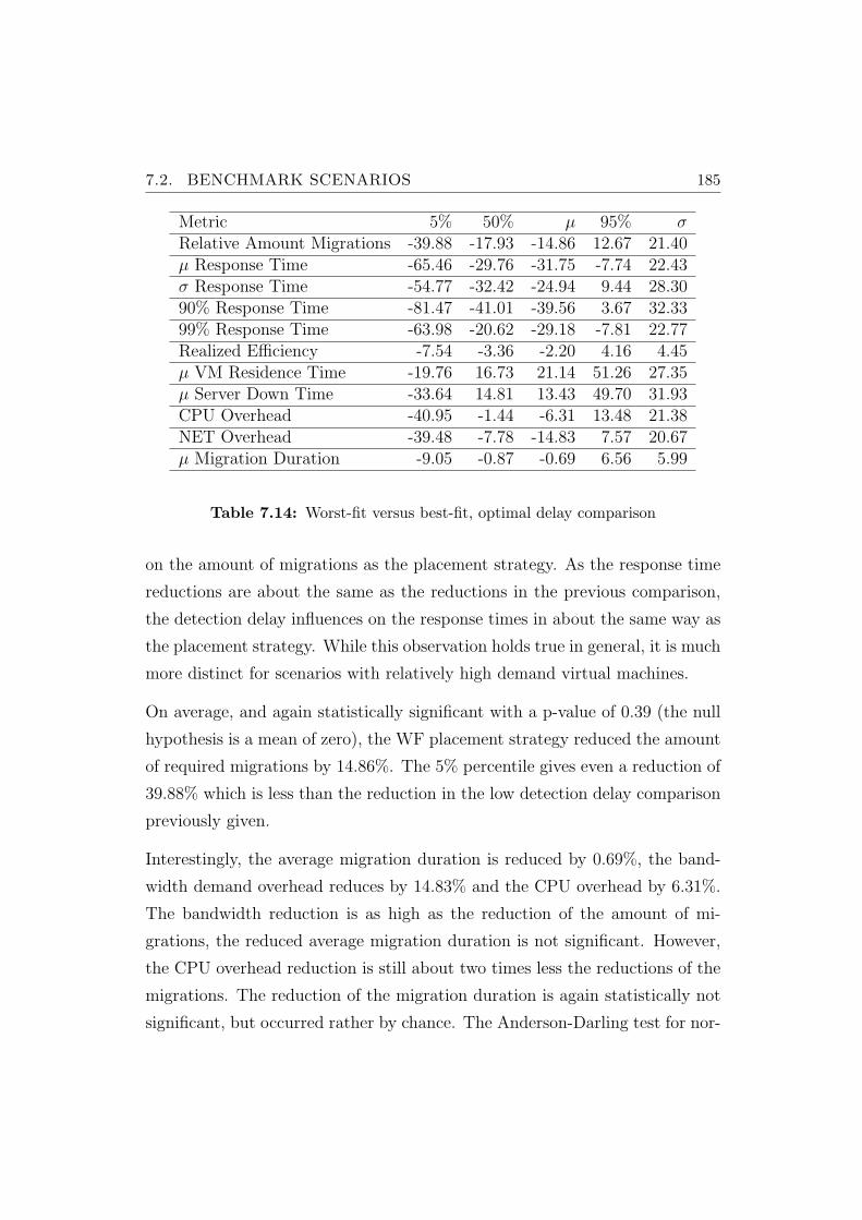
7.2. BENCHMARK SCENARIOS 185
Metric 5% 50% µ 95% σRelative Amount Migrations -39.88 -17.93 -14.86 12.67 21.40µ Response Time -65.46 -29.76 -31.75 -7.74 22.43σ Response Time -54.77 -32.42 -24.94 9.44 28.3090% Response Time -81.47 -41.01 -39.56 3.67 32.3399% Response Time -63.98 -20.62 -29.18 -7.81 22.77Realized Efficiency -7.54 -3.36 -2.20 4.16 4.45µ VM Residence Time -19.76 16.73 21.14 51.26 27.35µ Server Down Time -33.64 14.81 13.43 49.70 31.93CPU Overhead -40.95 -1.44 -6.31 13.48 21.38NET Overhead -39.48 -7.78 -14.83 7.57 20.67µ Migration Duration -9.05 -0.87 -0.69 6.56 5.99
Table 7.14: Worst-fit versus best-fit, optimal delay comparison
on the amount of migrations as the placement strategy. As the response time
reductions are about the same as the reductions in the previous comparison,
the detection delay influences on the response times in about the same way as
the placement strategy. While this observation holds true in general, it is much
more distinct for scenarios with relatively high demand virtual machines.
On average, and again statistically significant with a p-value of 0.39 (the null
hypothesis is a mean of zero), the WF placement strategy reduced the amount
of required migrations by 14.86%. The 5% percentile gives even a reduction of
39.88% which is less than the reduction in the low detection delay comparison
previously given.
Interestingly, the average migration duration is reduced by 0.69%, the band-
width demand overhead reduces by 14.83% and the CPU overhead by 6.31%.
The bandwidth reduction is as high as the reduction of the amount of mi-
grations, the reduced average migration duration is not significant. However,
the CPU overhead reduction is still about two times less the reductions of the
migrations. The reduction of the migration duration is again statistically not
significant, but occurred rather by chance. The Anderson-Darling test for nor-
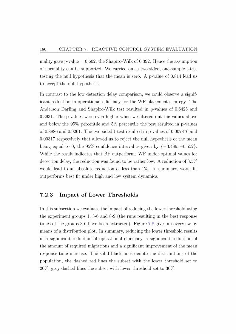
186 CHAPTER 7. REACTIVE CONTROL SYSTEM EVALUATION
mality gave p-value = 0.602, the Shapiro-Wilk of 0.392. Hence the assumption
of normality can be supported. We carried out a two sided, one-sample t-test
testing the null hypothesis that the mean is zero. A p-value of 0.814 lead us
to accept the null hypothesis.
In contrast to the low detection delay comparison, we could observe a signif-
icant reduction in operational efficiency for the WF placement strategy. The
Anderson Darling and Shapiro-Wilk test resulted in p-values of 0.6425 and
0.3931. The p-values were even higher when we filtered out the values above
and below the 95% percentile and 5% percentile the test resulted in p-values
of 0.8886 and 0.9261. The two-sided t-test resulted in p-values of 0.007876 and
0.00317 respectively that allowed us to reject the null hypothesis of the mean
being equal to 0, the 95% confidence interval is given by {−3.489,−0.552}.While the result indicates that BF outperforms WF under optimal values for
detection delay, the reduction was found to be rather low. A reduction of 3.5%
would lead to an absolute reduction of less than 1%. In summary, worst fit
outperforms best fit under high and low system dynamics.
7.2.3 Impact of Lower Thresholds
In this subsection we evaluate the impact of reducing the lower threshold using
the experiment groups 1, 3-6 and 8-9 (the runs resulting in the best response
times of the groups 3-6 have been extracted). Figure 7.8 gives an overview by
means of a distribution plot. In summary, reducing the lower threshold results
in a significant reduction of operational efficiency, a significant reduction of
the amount of required migrations and a significant improvement of the mean
response time increase. The solid black lines denote the distributions of the
population, the dashed red lines the subset with the lower threshold set to
20%, grey dashed lines the subset with lower threshold set to 30%.
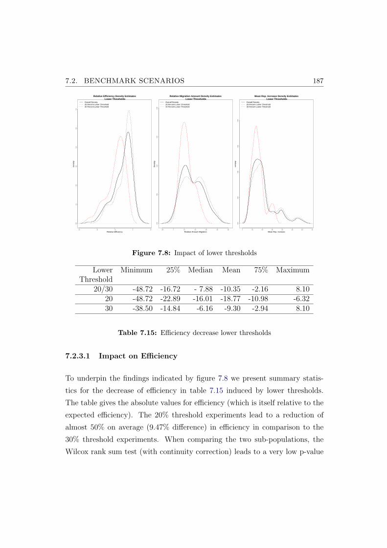
7.2. BENCHMARK SCENARIOS 187
−60 −40 −20 0 20
0.00
0.01
0.02
0.03
0.04
0.05
0.06
Relative Efficiency Density Estimates Lower Thresholds
Relative Efficiency
Den
sity
Overall Density20 Percent Lower Threshold30 Percent Lower Threshold
−100 0 100 200 300 400 500
0.00
00.
002
0.00
40.
006
0.00
8
Relative Migration Amount Density Estimates Lower Thresholds
Relative Amount Migration
Den
sity
Overall Density20 Percent Lower Threshold30 Percent Lower Threshold
0 100 200 300 400 500 600 700
0.00
00.
002
0.00
40.
006
0.00
8
Mean Rsp. Increase Density Estimates Lower Thresholds
Mean Rsp. Increase
Den
sity
Overall Density20 Percent Lower Threshold30 Percent Lower Threshold
Figure 7.8: Impact of lower thresholds
Lower Minimum 25% Median Mean 75% MaximumThreshold
20/30 -48.72 -16.72 - 7.88 -10.35 -2.16 8.1020 -48.72 -22.89 -16.01 -18.77 -10.98 -6.3230 -38.50 -14.84 -6.16 -9.30 -2.94 8.10
Table 7.15: Efficiency decrease lower thresholds
7.2.3.1 Impact on Efficiency
To underpin the findings indicated by figure 7.8 we present summary statis-
tics for the decrease of efficiency in table 7.15 induced by lower thresholds.
The table gives the absolute values for efficiency (which is itself relative to the
expected efficiency). The 20% threshold experiments lead to a reduction of
almost 50% on average (9.47% difference) in efficiency in comparison to the
30% threshold experiments. When comparing the two sub-populations, the
Wilcox rank sum test (with continuity correction) leads to a very low p-value
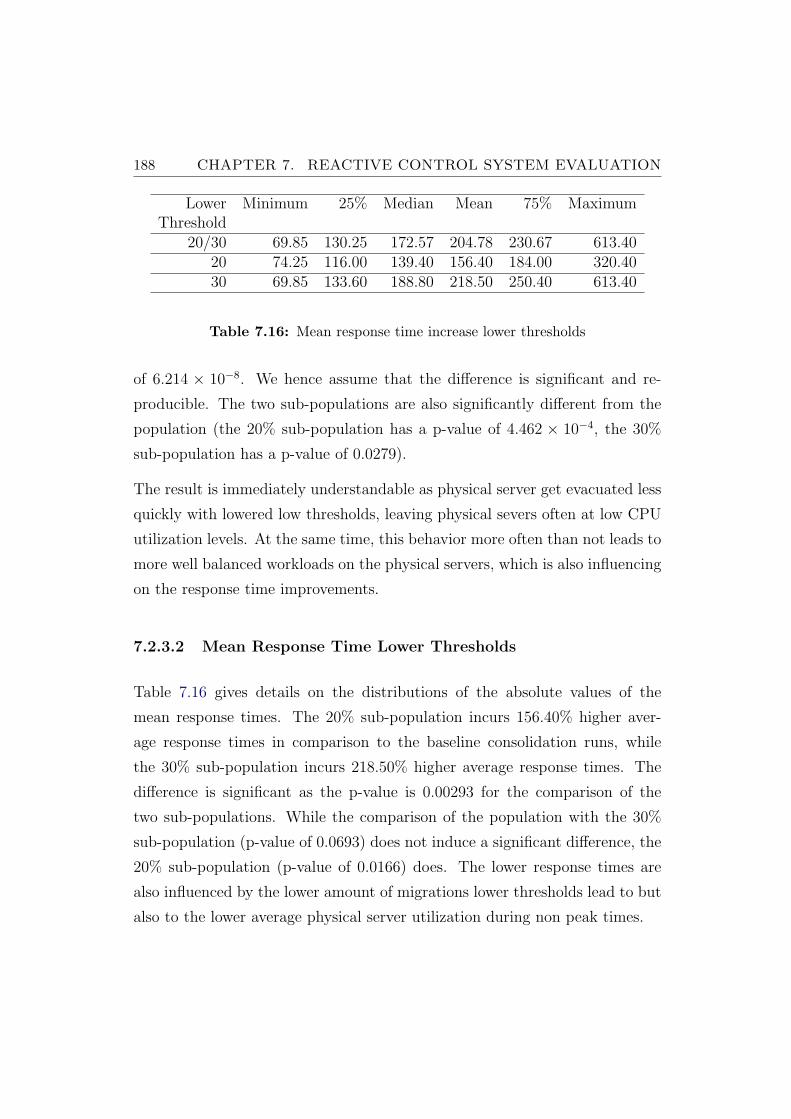
188 CHAPTER 7. REACTIVE CONTROL SYSTEM EVALUATION
Lower Minimum 25% Median Mean 75% MaximumThreshold
20/30 69.85 130.25 172.57 204.78 230.67 613.4020 74.25 116.00 139.40 156.40 184.00 320.4030 69.85 133.60 188.80 218.50 250.40 613.40
Table 7.16: Mean response time increase lower thresholds
of 6.214 × 10⁻⁸. We hence assume that the difference is significant and re-
producible. The two sub-populations are also significantly different from the
population (the 20% sub-population has a p-value of 4.462 × 10⁻⁴, the 30%
sub-population has a p-value of 0.0279).
The result is immediately understandable as physical server get evacuated less
quickly with lowered low thresholds, leaving physical severs often at low CPU
utilization levels. At the same time, this behavior more often than not leads to
more well balanced workloads on the physical servers, which is also influencing
on the response time improvements.
7.2.3.2 Mean Response Time Lower Thresholds
Table 7.16 gives details on the distributions of the absolute values of the
mean response times. The 20% sub-population incurs 156.40% higher aver-
age response times in comparison to the baseline consolidation runs, while
the 30% sub-population incurs 218.50% higher average response times. The
difference is significant as the p-value is 0.00293 for the comparison of the
two sub-populations. While the comparison of the population with the 30%
sub-population (p-value of 0.0693) does not induce a significant difference, the
20% sub-population (p-value of 0.0166) does. The lower response times are
also influenced by the lower amount of migrations lower thresholds lead to but
also to the lower average physical server utilization during non peak times.
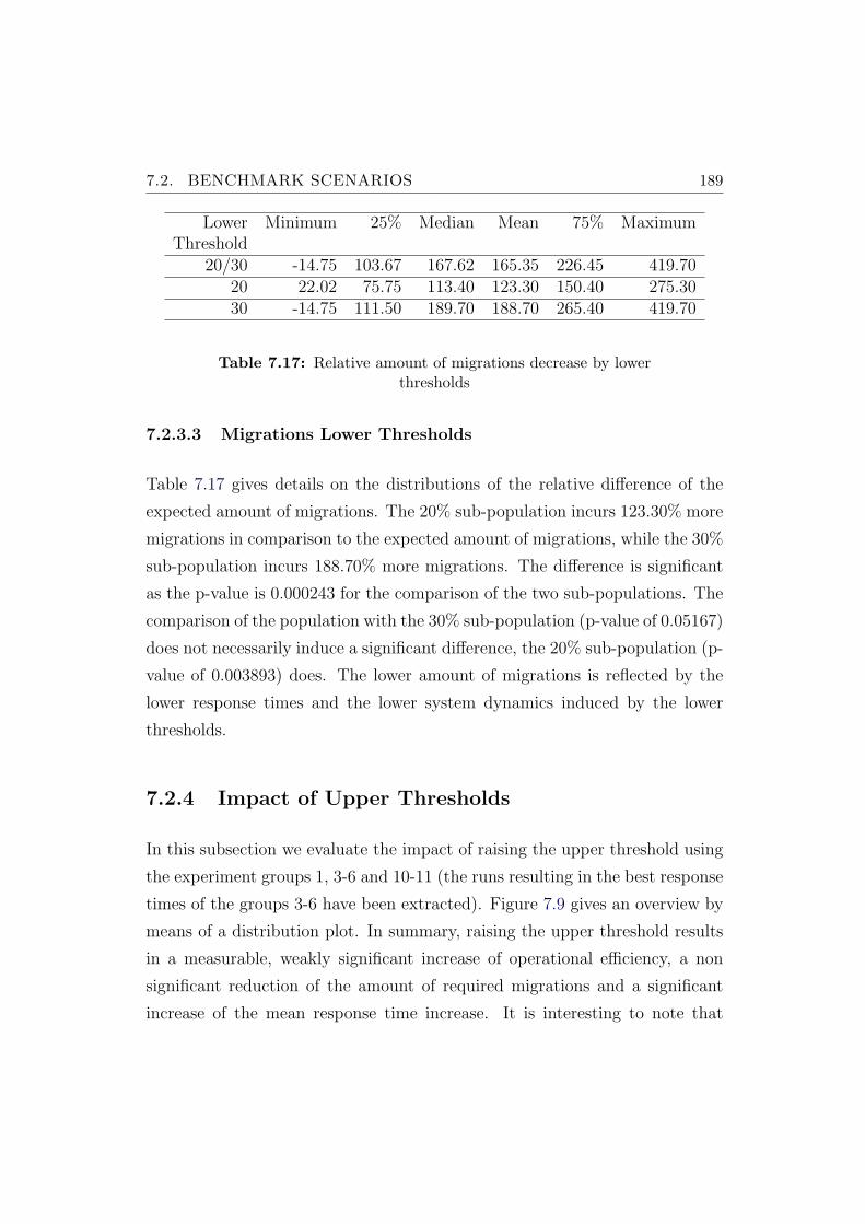
7.2. BENCHMARK SCENARIOS 189
Lower Minimum 25% Median Mean 75% MaximumThreshold
20/30 -14.75 103.67 167.62 165.35 226.45 419.7020 22.02 75.75 113.40 123.30 150.40 275.3030 -14.75 111.50 189.70 188.70 265.40 419.70
Table 7.17: Relative amount of migrations decrease by lowerthresholds
7.2.3.3 Migrations Lower Thresholds
Table 7.17 gives details on the distributions of the relative difference of the
expected amount of migrations. The 20% sub-population incurs 123.30% more
migrations in comparison to the expected amount of migrations, while the 30%
sub-population incurs 188.70% more migrations. The difference is significant
as the p-value is 0.000243 for the comparison of the two sub-populations. The
comparison of the population with the 30% sub-population (p-value of 0.05167)
does not necessarily induce a significant difference, the 20% sub-population (p-
value of 0.003893) does. The lower amount of migrations is reflected by the
lower response times and the lower system dynamics induced by the lower
thresholds.
7.2.4 Impact of Upper Thresholds
In this subsection we evaluate the impact of raising the upper threshold using
the experiment groups 1, 3-6 and 10-11 (the runs resulting in the best response
times of the groups 3-6 have been extracted). Figure 7.9 gives an overview by
means of a distribution plot. In summary, raising the upper threshold results
in a measurable, weakly significant increase of operational efficiency, a non
significant reduction of the amount of required migrations and a significant
increase of the mean response time increase. It is interesting to note that
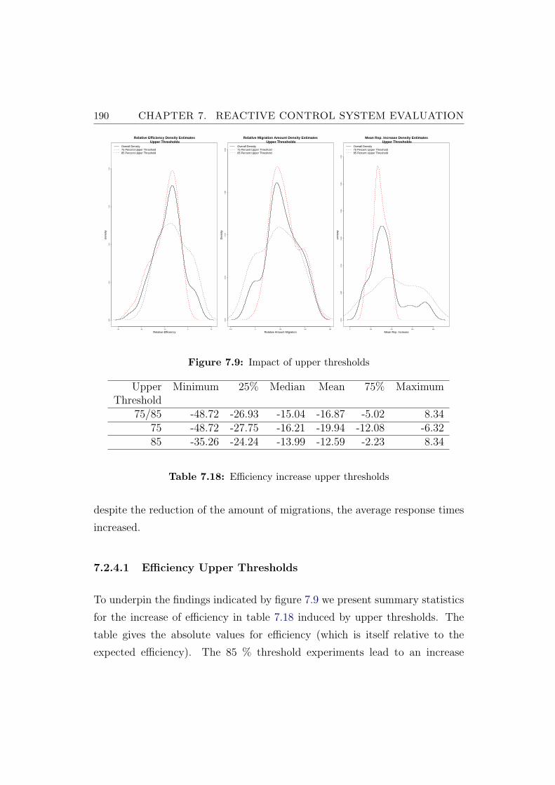
190 CHAPTER 7. REACTIVE CONTROL SYSTEM EVALUATION
−60 −40 −20 0 20
0.00
0.01
0.02
0.03
0.04
Relative Efficiency Density Estimates Upper Thresholds
Relative Efficiency
Den
sity
Overall Density75 Percent Upper Threshold85 Percent Upper Threshold
−100 0 100 200 300
0.00
00.
002
0.00
40.
006
0.00
8
Relative Migration Amount Density Estimates Upper Thresholds
Relative Amount Migration
Den
sity
Overall Density75 Percent Upper Threshold85 Percent Upper Threshold
0 100 200 300 400
0.00
00.
002
0.00
40.
006
0.00
80.
010
0.01
2
Mean Rsp. Increase Density Estimates Upper Thresholds
Mean Rsp. Increase
Den
sity
Overall Density75 Percent Upper Threshold85 Percent Upper Threshold
Figure 7.9: Impact of upper thresholds
Upper Minimum 25% Median Mean 75% MaximumThreshold
75/85 -48.72 -26.93 -15.04 -16.87 -5.02 8.3475 -48.72 -27.75 -16.21 -19.94 -12.08 -6.3285 -35.26 -24.24 -13.99 -12.59 -2.23 8.34
Table 7.18: Efficiency increase upper thresholds
despite the reduction of the amount of migrations, the average response times
increased.
7.2.4.1 Efficiency Upper Thresholds
To underpin the findings indicated by figure 7.9 we present summary statistics
for the increase of efficiency in table 7.18 induced by upper thresholds. The
table gives the absolute values for efficiency (which is itself relative to the
expected efficiency). The 85 % threshold experiments lead to an increase
7.2. BENCHMARK SCENARIOS 191
Upper Minimum 25% Median Mean 75% MaximumThreshold
75/85 -25.19 39.62 102.24 107.52 141.24 226.8075 22.02 75.64 109.80 119.70 150.90 226.8085 -25.19 23.53 86.76 90.84 158.00 225.80
Table 7.19: Relative amount of migrations decrease by upperthresholds
of almost 37% on average (7.35% difference) in efficiency in comparison to
the 75% threshold experiments. When comparing the two sub-populations,
the Wilcox rank sum test (with continuity correction) leads to a p-value of
0.07525. The p-value is rather low and does not allow us to speak about
significance. However, as an analysis of the different scenarios reveals, scenarios
with low average CPU utilization of the virtual machines benefit much more
than scenarios with larger mean CPU demands per virtual machine. When
we spilt the scenarios up into subgroups A (containing scenarios 1 - 6) and B
(containing scenarios 8 - 10) the difference becomes significant with a p-value
of 0.3273. We hence assume that the difference is significant and reproducible
for different types of workload scenarios.
7.2.4.2 Migrations Upper Thresholds
Table 7.19 gives details on the distributions of the relative difference of the
expected amount of migrations. The 85% sub-population incurs 90.84% more
migrations in comparison to the expected amount of migrations (derived with
85% maximum capacity), while the 75% sub-population incurs 119.70% more
migrations. The difference is statistically significant as the p-value is 0.1937
for the comparison of the two sub-populations. When we spilt the scenarios up
into subgroups A (containing scenarios 1 - 6) and B (containing scenarios 8 -
10) the difference becomes even more significant with a p-value of 0.2749. We
hence assume that the difference is significant and reproducible for different
192 CHAPTER 7. REACTIVE CONTROL SYSTEM EVALUATION
types of workload scenarios. Subgroup A scenarios again benefit more than
subgroup B scenarios.
7.2.4.3 Response Time Upper Thresholds
Table 7.20 gives details on the distributions of the absolute values of the mean
response times. The 75% sub-population incurs 143.40% higher average re-
sponse times in comparison to the baseline consolidation runs, while the 85%
sub-population incurs 221.20% higher average response times. The difference
is not significant as the p-value is 0.002814 for the comparison of the two sub-
populations. The higher response times are mainly influenced by the higher
Upper Minimum 25% Median Mean 75% MaximumThreshold
75/85 53.16 149.25 174.26 200.40 230.57 393.5075 77.52 125.80 139.20 143.40 167.20 201.8085 53.16 158.90 200.60 221.20 305.20 393.50
Table 7.20: Mean response time increase upper thresholds
workload density and the well known, non-linear response time increase effect
at high physical server utilization levels. When we spilt the scenarios up into
subgroups A (containing scenarios 1 - 6) and B (containing scenarios 8 - 10)
the difference becomes significant with a p-value of 0.3806. We hence assume
that the difference is significant and reproducible for different types of work-
load scenarios. Subgroup A scenarios again benefit more than subgroup B
scenarios.
7.2.4.4 Scenario Analysis of Upper Thresholds
In table 7.21 we give an analysis of the impact of increasing the upper threshold
from 75 to 85% for all seven scenarios. The comparison given in the table is
7.2. BENCHMARK SCENARIOS 193
a relative comparison of the averages values of the experiment runs in the
experiment groups 8, 9, 10 and 11 with 75 and 85% upper thresholds, 20%
lower threshold, with a detection delay of one and the optimal detection delay
for each scenario (with respect to the mean response time). All entries in table
7.21 are percent values.
While increasing the upper thresholds leads to a decrease of required migra-
tions for almost all scenarios and detection delays (between 193.90 and 5.18%),
all response time related metrics increase except for scenario 1 that is made
up of the smallest virtual machines with respect to the average CPU demand
of the virtual machines. The result shows that the 75% threshold is a reason-
able setting for scenarios with large capacitated virtual machines, the 85% is
well suited for scenarios with low capacitated virtual machines. The increase
in response times is due to high resource utilization on the physical servers
and intense overloads caused by insufficient spare CPU time for executing live
migrations. The adverse effect of live migrations is becoming more significant
in these scenarios.
Except for scenario 5 the realized efficiency increased with a tendency for
higher gains for scenarios with higher average resource demands, however, the
relative improvements range between 4.03 and 22.72% and can be considered
marginal in absolute numbers.
7.2.5 Detection Delay
In this subsection we analyze the impact of the detection delay on the migra-
tions, response time and efficiency metrics. For our comparison we use the
runs of the experiment groups 1, 3-6 for the 9 complete scenarios with the
(30/75/WF) experiment configuration.
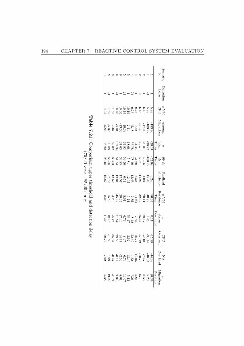
194 CHAPTER 7. REACTIVE CONTROL SYSTEM EVALUATION
Scen
ario
Detectio
nµ
VM
Am
ount
µ99
%R
ealized
µV
Mµ
CP
UN
etµ
IdD
elay
CP
UM
igra
tion
sR
sp.
Rsp
.E
fficien
cyR
esiden
ceS
erver
Overh
ead
Overh
ead
Mig
ratio
nT
imes
Tim
esT
ime
Dow
ntim
eD
ura
tion
11
5.9
9-1
93.9
0-2
8.3
7-5
2.6
86.2
456.0
40.1
1-1
5.9
8-4
4.0
920.3
41
24
5.9
9-1
09.2
2-3
8.7
4-1
00.7
915.4
440.9
91.4
5-3
3.1
4-4
6.8
45.2
32
16.4
8-1
7.9
020.0
746.5
64.0
320.1
138.1
7-2
.10
-7.4
78.5
62
36
6.4
8-5
1.4
942.5
153.7
111.2
432.5
235.4
4-5
0.1
9-1
0.7
515.7
04
19.2
50.5
231.4
431.6
06.5
2-1
1.6
4-7
.65
18.7
712.0
65.8
44
24
9.2
5-5
.18
56.7
878.1
013.4
5-2
.85
-18.1
222.4
94.8
27.2
15
110.1
92.4
118.0
85.8
1-1
2.9
5-6
.24
-53.1
73.6
2-1
3.4
6-5
.13
524
10.1
9-1
0.3
364.9
359.5
0-6
.51
8.0
76.7
6-8
.67
-6.7
3-1
3.0
76
110.4
0-1
3.3
331.6
334.2
517.5
728.3
537.4
414.1
1-2
.50
8.6
16
24
10.4
0-5
.81
102.3
451.5
413.8
145.8
931.5
729.5
6-0
.14
9.0
48
111.5
52.4
662.0
260.0
313.5
24.2
0-6
.77
35.6
7-0
.47
-7.3
98
24
11.5
5-5
.32
90.8
866.5
822.7
215.8
918.4
651.8
98.9
819.2
210
114.9
5-6
.86
98.2
293.4
816.8
78.0
411.3
529.7
27.9
25.3
8
Tab
le7.21:
Com
parisonupper
thresholdand
detectiondelay
(75/20versus
85/20)in
%
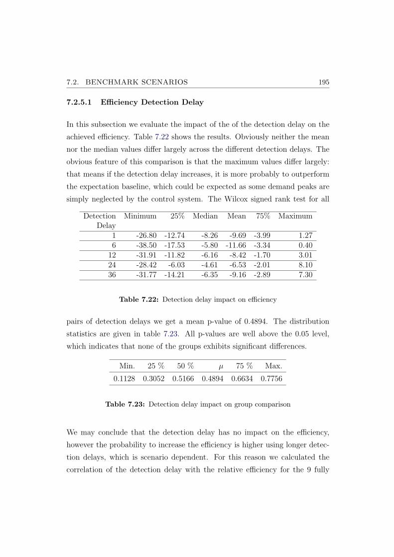
7.2. BENCHMARK SCENARIOS 195
7.2.5.1 Efficiency Detection Delay
In this subsection we evaluate the impact of the of the detection delay on the
achieved efficiency. Table 7.22 shows the results. Obviously neither the mean
nor the median values differ largely across the different detection delays. The
obvious feature of this comparison is that the maximum values differ largely:
that means if the detection delay increases, it is more probably to outperform
the expectation baseline, which could be expected as some demand peaks are
simply neglected by the control system. The Wilcox signed rank test for all
Detection Minimum 25% Median Mean 75% MaximumDelay
1 -26.80 -12.74 -8.26 -9.69 -3.99 1.276 -38.50 -17.53 -5.80 -11.66 -3.34 0.40
12 -31.91 -11.82 -6.16 -8.42 -1.70 3.0124 -28.42 -6.03 -4.61 -6.53 -2.01 8.1036 -31.77 -14.21 -6.35 -9.16 -2.89 7.30
Table 7.22: Detection delay impact on efficiency
pairs of detection delays we get a mean p-value of 0.4894. The distribution
statistics are given in table 7.23. All p-values are well above the 0.05 level,
which indicates that none of the groups exhibits significant differences.
Min. 25 % 50 % µ 75 % Max.
0.1128 0.3052 0.5166 0.4894 0.6634 0.7756
Table 7.23: Detection delay impact on group comparison
We may conclude that the detection delay has no impact on the efficiency,
however the probability to increase the efficiency is higher using longer detec-
tion delays, which is scenario dependent. For this reason we calculated the
correlation of the detection delay with the relative efficiency for the 9 fully
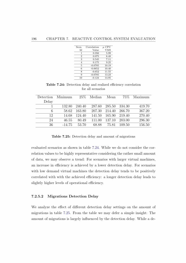
196 CHAPTER 7. REACTIVE CONTROL SYSTEM EVALUATION
Scen. Correlation µ CPUId Value VMS1 0.356 5.992 0.075 6.483 0.545 7.114 0.175 9.255 -0.0785 10.196 -0.0652 10.408 -0.652 11.559 -0.0785 13.23
10 -0.124 14.95
Table 7.24: Detection delay and realized efficiency correlationfor all scenarios
Detection Minimum 25% Median Mean 75% MaximumDelay
1 132.80 240.40 287.60 285.50 334.30 419.706 58.62 163.80 207.30 214.40 266.70 367.20
12 14.68 124.40 141.50 165.90 219.40 270.4024 46.55 80.49 111.00 137.10 203.00 296.3036 -14.75 53.70 68.88 75.81 109.50 156.50
Table 7.25: Detection delay and amount of migrations
evaluated scenarios as shown in table 7.24. While we do not consider the cor-
relation values to be highly representative considering the rather small amount
of data, we may observe a trend: For scenarios with larger virtual machines,
an increase in efficiency is achieved by a lower detection delay. For scenarios
with low demand virtual machines the detection delay tends to be positively
correlated with with the achieved efficiency: a longer detection delay leads to
slightly higher levels of operational efficiency.
7.2.5.2 Migrations Detection Delay
We analyze the effect of different detection delay settings on the amount of
migrations in table 7.25. From the table we may defer a simple insight: The
amount of migrations is largely influenced by the detection delay. While a de-
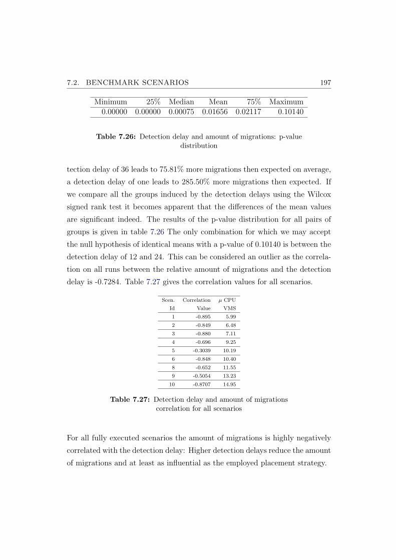
7.2. BENCHMARK SCENARIOS 197
Minimum 25% Median Mean 75% Maximum0.00000 0.00000 0.00075 0.01656 0.02117 0.10140
Table 7.26: Detection delay and amount of migrations: p-valuedistribution
tection delay of 36 leads to 75.81% more migrations then expected on average,
a detection delay of one leads to 285.50% more migrations then expected. If
we compare all the groups induced by the detection delays using the Wilcox
signed rank test it becomes apparent that the differences of the mean values
are significant indeed. The results of the p-value distribution for all pairs of
groups is given in table 7.26 The only combination for which we may accept
the null hypothesis of identical means with a p-value of 0.10140 is between the
detection delay of 12 and 24. This can be considered an outlier as the correla-
tion on all runs between the relative amount of migrations and the detection
delay is -0.7284. Table 7.27 gives the correlation values for all scenarios.
Scen. Correlation µ CPU
Id Value VMS
1 -0.895 5.99
2 -0.849 6.48
3 -0.880 7.11
4 -0.696 9.25
5 -0.3039 10.19
6 -0.848 10.40
8 -0.652 11.55
9 -0.5054 13.23
10 -0.8707 14.95
Table 7.27: Detection delay and amount of migrationscorrelation for all scenarios
For all fully executed scenarios the amount of migrations is highly negatively
correlated with the detection delay: Higher detection delays reduce the amount
of migrations and at least as influential as the employed placement strategy.
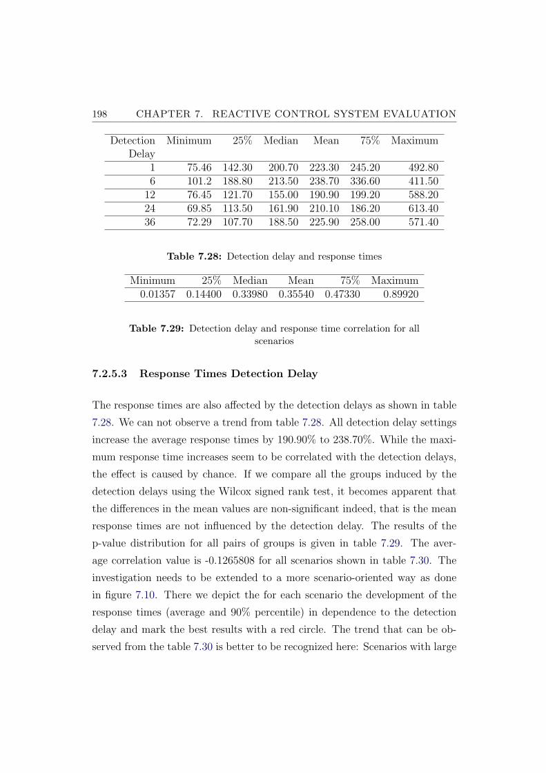
198 CHAPTER 7. REACTIVE CONTROL SYSTEM EVALUATION
Detection Minimum 25% Median Mean 75% MaximumDelay
1 75.46 142.30 200.70 223.30 245.20 492.806 101.2 188.80 213.50 238.70 336.60 411.50
12 76.45 121.70 155.00 190.90 199.20 588.2024 69.85 113.50 161.90 210.10 186.20 613.4036 72.29 107.70 188.50 225.90 258.00 571.40
Table 7.28: Detection delay and response times
Minimum 25% Median Mean 75% Maximum0.01357 0.14400 0.33980 0.35540 0.47330 0.89920
Table 7.29: Detection delay and response time correlation for allscenarios
7.2.5.3 Response Times Detection Delay
The response times are also affected by the detection delays as shown in table
7.28. We can not observe a trend from table 7.28. All detection delay settings
increase the average response times by 190.90% to 238.70%. While the maxi-
mum response time increases seem to be correlated with the detection delays,
the effect is caused by chance. If we compare all the groups induced by the
detection delays using the Wilcox signed rank test, it becomes apparent that
the differences in the mean values are non-significant indeed, that is the mean
response times are not influenced by the detection delay. The results of the
p-value distribution for all pairs of groups is given in table 7.29. The aver-
age correlation value is -0.1265808 for all scenarios shown in table 7.30. The
investigation needs to be extended to a more scenario-oriented way as done
in figure 7.10. There we depict the for each scenario the development of the
response times (average and 90% percentile) in dependence to the detection
delay and mark the best results with a red circle. The trend that can be ob-
served from the table 7.30 is better to be recognized here: Scenarios with large

7.2. BENCHMARK SCENARIOS 199
Scen. Correlation µ CPUId Value VMS1 -0.4044 5.992 -0.319 6.483 -0.567 7.114 -0.34 9.255 0.315 10.196 -0.238 10.408 -0.0393 11.559 0.039 13.23
10 0.591 14.95
Table 7.30: Detection delay and response time correlation for allscenarios
6070
8090
100
Scenario Mean VM CPU Demand: 5.99
Detection Delay
Mea
n R
sp. T
ime
Incr
ease
1 6 12 24 36
●
●
Mean Rsp.90−Perc. Rsp.
100
150
200
250
300
Scenario Mean VM CPU Demand: 6.48
Detection Delay
Mea
n R
sp. T
ime
Incr
ease
1 6 12 24 36
●
●
Mean Rsp.90−Perc. Rsp.
7080
9010
012
0
Scenario Mean VM CPU Demand: 7.11
Detection Delay
Mea
n R
sp. T
ime
Incr
ease
1 6 12 24 36
●●
Mean Rsp.90−Perc. Rsp.
120
160
200
Scenario Mean VM CPU Demand: 9.25
Detection Delay
Mea
n R
sp. T
ime
Incr
ease
1 6 12 24 36
●
●
Mean Rsp.90−Perc. Rsp.
150
200
250
300
Scenario Mean VM CPU Demand: 10.19
Detection Delay
Mea
n R
sp. T
ime
Incr
ease
1 6 12 24 36
●
●
Mean Rsp.90−Perc. Rsp.
200
250
300
350
Scenario Mean VM CPU Demand: 10.4
Detection Delay
Mea
n R
sp. T
ime
Incr
ease
1 6 12 24 36
●
●
Mean Rsp.90−Perc. Rsp.
100
150
200
250
300
Scenario Mean VM CPU Demand: 11.55
Detection Delay
Mea
n R
sp. T
ime
Incr
ease
1 6 12 24 36
●
●
Mean Rsp.90−Perc. Rsp.
300
350
400
450
500
Scenario Mean VM CPU Demand: 13.23
Detection Delay
Mea
n R
sp. T
ime
Incr
ease
1 6 12 24 36
● ●
Mean Rsp.90−Perc. Rsp.
400
500
600
Scenario Mean VM CPU Demand: 14.95
Detection Delay
Mea
n R
sp. T
ime
Incr
ease
1 6 12 24 36
●●
Mean Rsp.90−Perc. Rsp.
Figure 7.10: Response time versus detection delay
200 CHAPTER 7. REACTIVE CONTROL SYSTEM EVALUATION
relative virtual machine resource demands benefit from rather short detection
delays. While migrations are more costly for these scenarios, it is better to
initiate migrations in a highly reactive way as overload situations are much
more problematic for these scenarios, leading to response time degradation.
7.2.6 Main Findings
We have shown that reactive control is about to deliver expectable operational
efficiency but incurs response time penalties compared to less efficient static
consolidation. As we did not treat main memory as a dynamically assignable
or sharable resource, some of our scenarios suffered from main memory induced
efficiency deadlocks that caused negative deviations from these efficiency re-
sults.
Besides the negative effects live migration have on the application performance
of hosted applications, higher levels of sever utilization and consolidation ef-
fects increase the response times for dynamic workload management. The
effects of live migrations diminish as more low demand virtual machines are
managed. Scenarios with high demand virtual machines are affected much
more by these effects.
Reactive control initiates on average about 170% more live migrations than re-
quired to achieve the expected efficiency, which is caused by system oscillations
and overly reactive control system settings. While the detection delay has no
impact on operational efficiency from a statistical point of view for all exper-
iments, the probability to increase the efficiency is, for some scenarios higher
using higher detection delays. This would indicate that longer detection delays
are preferable over shorter ones as longer ones also reduced the amount of live
migrations significantly. However, short detection delays deliver best results
for scenarios with virtual machines with relatively large resource demands.
We also found hat the worst fit virtual machine placement strategy outper-
7.3. IMPROVEMENTS BY PROPER PARAMETER SELECTION 201
forms the best fit strategy for almost all metrics of interest. All response time
related metrics improve between 24.76 and 40.35%, a reduction in operational
efficiency for the worst fit placement strategy could not be observed and on
average, and statistically significant, the worst t placement strategy reduced
the amount of required migrations by 19.42%.
Reducing the lower threshold results in a reduction of operational efficiency,
a significant reduction of the amount of required migrations and a signifi-
cant improvement of the mean response time increase, while raising the upper
threshold results in a measurable increase of operational efficiency, a non sig-
nificant reduction of the amount of required migrations and an increase of the
mean response time increase.
These general statements are important to tune reactive control systems. In
the next section we will show that bad parameter selection leads to adverse
control system performance in terms of system stability and application per-
formance. However, efficiency is not affected in the same way as the amount
of migrations and application response times.
7.3 Improvements by Proper Parameter Se-
lection
We have discussed the effects of the various control parameters on some per-
formance metrics and have seen that the performance of reactive control varies
significantly for different parameter configurations and their combinations. In
the following subsections we will show the actual differences on a per sce-
nario basis. To highlight the importance of proper control system parameter
selection we compare the average of the experiment runs of an experiment con-
figuration that delivered best and worst results with respect to a given metric
(average response time, amount of migrations and efficiency). Results will be
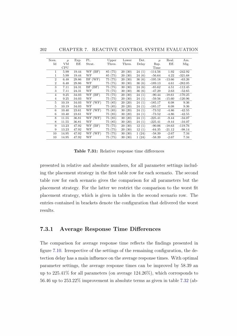
202 CHAPTER 7. REACTIVE CONTROL SYSTEM EVALUATION
Scen. µ Exp. Pl.. Upper Lower Det. µ Real. Am.Id VM Eff. Strat. Thres. Thres. Delay Rsp. Eff. Mig.
CPU Time1 5.99 19.44 WF (BF) 85 (75) 20 (30) 24 (1) -114.56 1.92 -242.921 5.99 19.44 WF 85 (75) 20 (30) 24 (6) -56.64 4.22 -321.682 6.48 29.86 BF (WF) 75 (75) 20 (30) 36 (6) -195.18 -13.66 -63.262 6.48 29.86 WF 75 (75) 30 (30) 36 (6) -189.13 4.61 -282.053 7.11 24.31 BF (BF) 75 (75) 30 (30) 24 (6) -85.62 4.51 -112.453 7.11 24.31 WF 75 (75) 30 (30) 36 (6) -47.29 2.63 -52.654 9.25 34.03 WF (BF) 75 (75) 20 (30) 24 (1) -90.44 -18.61 -170.254 9.25 34.03 WF 75 (75) 20 (30) 24 (1) -59.56 -15.60 -120.965 10.19 34.03 WF (WF) 75 (85) 20 (20) 24 (1) -185.17 6.08 9.365 10.19 34.03 WF 75 (85) 20 (20) 24 (1) -185.17 6.08 9.366 10.40 23.61 WF (WF) 75 (85) 30 (20) 24 (1) -73.52 -4.86 -42.556 10.40 23.61 WF 75 (85) 30 (20) 24 (1) -73.52 -4.86 -42.558 11.55 36.81 WF (WF) 75 (85) 30 (20) 24 (1) -225.41 -9.44 -34.078 11.55 36.81 WF 75 (85) 30 (20) 24 (1) -225.41 -9.44 -34.079 13.23 47.92 WF (BF) 75 (75) 20 (30) 12 (1) -90.06 -18.63 -119.769 13.23 47.92 WF 75 (75) 20 (30) 12 (1) -64.35 -21.12 -98.14
10 14.95 47.92 WF (WF) 75 (75) 30 (30) 1 (24) -58.39 -2.67 7.3410 14.95 47.92 WF 75 (75) 30 (30) 1 (24) -58.39 -2.67 7.34
Table 7.31: Relative response time differences
presented in relative and absolute numbers, for all parameter settings includ-
ing the placement strategy in the first table row for each scenario. The second
table row for each scenario gives the comparison for all parameters but the
placement strategy. For the latter we restrict the comparison to the worst fit
placement strategy, which is given in tables in the second scenario row. The
entries contained in brackets denote the configuration that delivered the worst
results.
7.3.1 Average Response Time Differences
The comparison for average response time reflects the findings presented in
figure 7.10. Irrespective of the settings of the remaining configuration, the de-
tection delay has a main influence on the average response times. With optimal
parameter settings, the average response times can be improved by 58.39 an
up to 225.41% for all parameters (on average 124.26%), which corresponds to
56.46 up to 253.22% improvement in absolute terms as given in table 7.32 (ab-
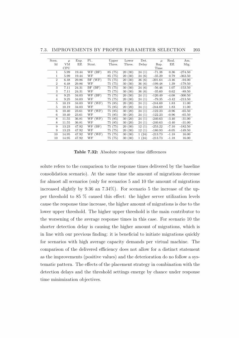
7.3. IMPROVEMENTS BY PROPER PARAMETER SELECTION 203
Scen. µ Exp. Pl.. Upper Lower Det. µ Real. Am.Id VM Eff. Strat. Thres. Thres. Delay Rsp. Eff. Mig.
CPU Time1 5.99 19.44 WF (BF) 85 (75) 20 (30) 24 (1) -71.38 0.36 -274.501 5.99 19.44 WF 85 (75) 20 (30) 24 (6) -35.29 0.79 -363.502 6.48 29.86 BF (WF) 75 (75) 20 (30) 36 (6) -201.64 -3.46 -94.002 6.48 29.86 WF 75 (75) 30 (30) 36 (6) -199.48 1.39 -179.503 7.11 24.31 BF (BF) 75 (75) 30 (30) 24 (6) -56.46 1.07 -153.503 7.11 24.31 WF 75 (75) 30 (30) 36 (6) -35.60 0.62 -89.504 9.25 34.03 WF (BF) 75 (75) 20 (30) 24 (1) -120.49 -4.08 -300.504 9.25 34.03 WF 75 (75) 20 (30) 24 (1) -79.35 -3.42 -213.505 10.19 34.03 WF (WF) 75 (85) 20 (20) 24 (1) -244.69 1.83 11.005 10.19 34.03 WF 75 (85) 20 (20) 24 (1) -244.69 1.83 11.006 10.40 23.61 WF (WF) 75 (85) 30 (20) 24 (1) -122.23 -0.96 -65.506 10.40 23.61 WF 75 (85) 30 (20) 24 (1) -122.23 -0.96 -65.508 11.55 36.81 WF (WF) 75 (85) 30 (20) 24 (1) -240.63 -3.40 -31.008 11.55 36.81 WF 75 (85) 30 (20) 24 (1) -240.63 -3.40 -31.009 13.23 47.92 WF (BF) 75 (75) 20 (30) 12 (1) -253.22 -7.10 -182.509 13.23 47.92 WF 75 (75) 20 (30) 12 (1) -180.93 -8.05 -149.50
10 14.95 47.92 WF (WF) 75 (75) 30 (30) 1 (24) -213.73 -1.18 16.0010 14.95 47.92 WF 75 (75) 30 (30) 1 (24) -213.73 -1.18 16.00
Table 7.32: Absolute response time differences
solute refers to the comparison to the response times delivered by the baseline
consolidation scenario). At the same time the amount of migrations decrease
for almost all scenarios (only for scenarios 5 and 10 the amount of migrations
increased slightly by 9.36 an 7.34%). For scenario 5 the increase of the up-
per threshold to 85 % caused this effect: the higher server utilization levels
cause the response time increase, the higher amount of migrations is due to the
lower upper threshold. The higher upper threshold is the main contributor to
the worsening of the average response times in this case. For scenario 10 the
shorter detection delay is causing the higher amount of migrations, which is
in line with our previous finding: it is beneficial to initiate migrations quickly
for scenarios with high average capacity demands per virtual machine. The
comparison of the delivered efficiency does not allow for a distinct statement
as the improvements (positive values) and the deterioration do no follow a sys-
tematic pattern. The effects of the placement strategy in combination with the
detection delays and the threshold settings emerge by chance under response
time minimization objectives.
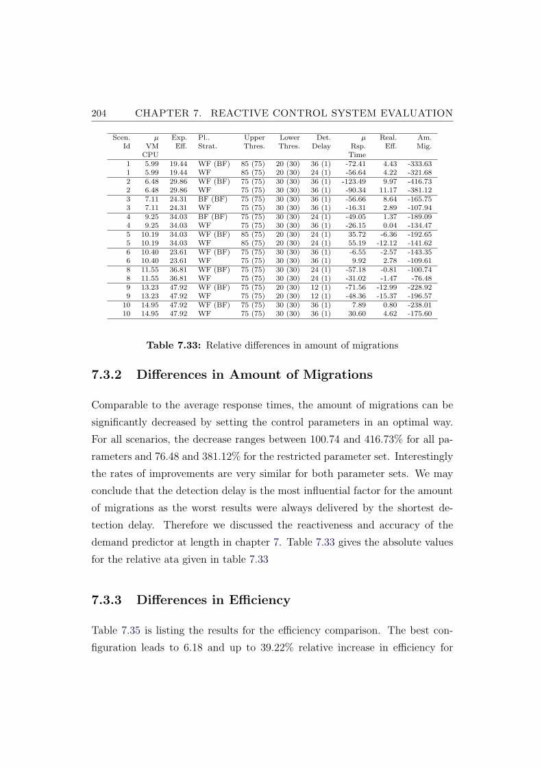
204 CHAPTER 7. REACTIVE CONTROL SYSTEM EVALUATION
Scen. µ Exp. Pl.. Upper Lower Det. µ Real. Am.Id VM Eff. Strat. Thres. Thres. Delay Rsp. Eff. Mig.
CPU Time1 5.99 19.44 WF (BF) 85 (75) 20 (30) 36 (1) -72.41 4.43 -333.631 5.99 19.44 WF 85 (75) 20 (30) 24 (1) -56.64 4.22 -321.682 6.48 29.86 WF (BF) 75 (75) 30 (30) 36 (1) -123.49 9.97 -416.732 6.48 29.86 WF 75 (75) 30 (30) 36 (1) -90.34 11.17 -381.123 7.11 24.31 BF (BF) 75 (75) 30 (30) 36 (1) -56.66 8.64 -165.753 7.11 24.31 WF 75 (75) 30 (30) 36 (1) -16.31 2.89 -107.944 9.25 34.03 BF (BF) 75 (75) 30 (30) 24 (1) -49.05 1.37 -189.094 9.25 34.03 WF 75 (75) 30 (30) 36 (1) -26.15 0.04 -134.475 10.19 34.03 WF (BF) 85 (75) 20 (30) 24 (1) 35.72 -6.36 -192.655 10.19 34.03 WF 85 (75) 20 (30) 24 (1) 55.19 -12.12 -141.626 10.40 23.61 WF (BF) 75 (75) 30 (30) 36 (1) -6.55 -2.57 -143.356 10.40 23.61 WF 75 (75) 30 (30) 36 (1) 9.92 2.78 -109.618 11.55 36.81 WF (BF) 75 (75) 30 (30) 24 (1) -57.18 -0.81 -100.748 11.55 36.81 WF 75 (75) 30 (30) 24 (1) -31.02 -1.47 -76.489 13.23 47.92 WF (BF) 75 (75) 20 (30) 12 (1) -71.56 -12.99 -228.929 13.23 47.92 WF 75 (75) 20 (30) 12 (1) -48.36 -15.37 -196.57
10 14.95 47.92 WF (BF) 75 (75) 30 (30) 36 (1) 7.89 0.80 -238.0110 14.95 47.92 WF 75 (75) 30 (30) 36 (1) 30.60 4.62 -175.60
Table 7.33: Relative differences in amount of migrations
7.3.2 Differences in Amount of Migrations
Comparable to the average response times, the amount of migrations can be
significantly decreased by setting the control parameters in an optimal way.
For all scenarios, the decrease ranges between 100.74 and 416.73% for all pa-
rameters and 76.48 and 381.12% for the restricted parameter set. Interestingly
the rates of improvements are very similar for both parameter sets. We may
conclude that the detection delay is the most influential factor for the amount
of migrations as the worst results were always delivered by the shortest de-
tection delay. Therefore we discussed the reactiveness and accuracy of the
demand predictor at length in chapter 7. Table 7.33 gives the absolute values
for the relative ata given in table 7.33
7.3.3 Differences in Efficiency
Table 7.35 is listing the results for the efficiency comparison. The best con-
figuration leads to 6.18 and up to 39.22% relative increase in efficiency for
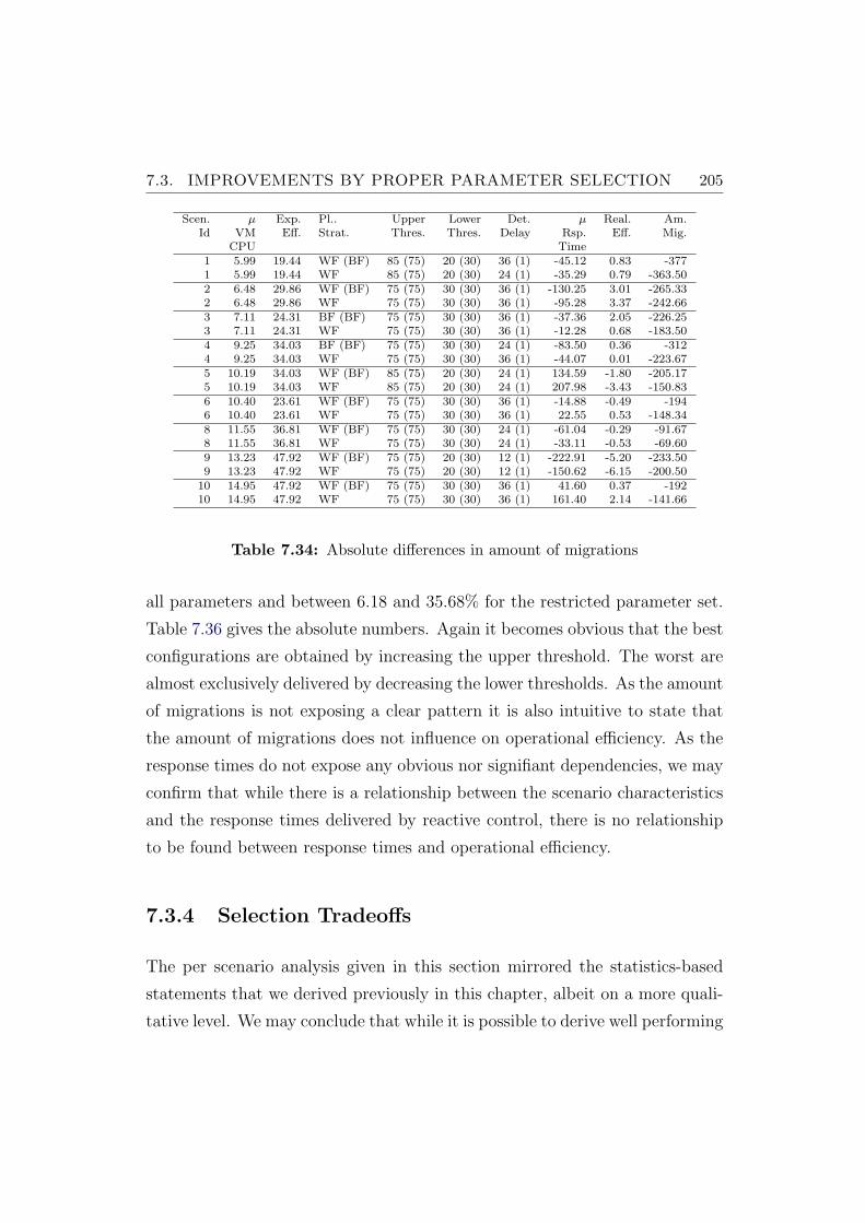
7.3. IMPROVEMENTS BY PROPER PARAMETER SELECTION 205
Scen. µ Exp. Pl.. Upper Lower Det. µ Real. Am.Id VM Eff. Strat. Thres. Thres. Delay Rsp. Eff. Mig.
CPU Time1 5.99 19.44 WF (BF) 85 (75) 20 (30) 36 (1) -45.12 0.83 -3771 5.99 19.44 WF 85 (75) 20 (30) 24 (1) -35.29 0.79 -363.502 6.48 29.86 WF (BF) 75 (75) 30 (30) 36 (1) -130.25 3.01 -265.332 6.48 29.86 WF 75 (75) 30 (30) 36 (1) -95.28 3.37 -242.663 7.11 24.31 BF (BF) 75 (75) 30 (30) 36 (1) -37.36 2.05 -226.253 7.11 24.31 WF 75 (75) 30 (30) 36 (1) -12.28 0.68 -183.504 9.25 34.03 BF (BF) 75 (75) 30 (30) 24 (1) -83.50 0.36 -3124 9.25 34.03 WF 75 (75) 30 (30) 36 (1) -44.07 0.01 -223.675 10.19 34.03 WF (BF) 85 (75) 20 (30) 24 (1) 134.59 -1.80 -205.175 10.19 34.03 WF 85 (75) 20 (30) 24 (1) 207.98 -3.43 -150.836 10.40 23.61 WF (BF) 75 (75) 30 (30) 36 (1) -14.88 -0.49 -1946 10.40 23.61 WF 75 (75) 30 (30) 36 (1) 22.55 0.53 -148.348 11.55 36.81 WF (BF) 75 (75) 30 (30) 24 (1) -61.04 -0.29 -91.678 11.55 36.81 WF 75 (75) 30 (30) 24 (1) -33.11 -0.53 -69.609 13.23 47.92 WF (BF) 75 (75) 20 (30) 12 (1) -222.91 -5.20 -233.509 13.23 47.92 WF 75 (75) 20 (30) 12 (1) -150.62 -6.15 -200.50
10 14.95 47.92 WF (BF) 75 (75) 30 (30) 36 (1) 41.60 0.37 -19210 14.95 47.92 WF 75 (75) 30 (30) 36 (1) 161.40 2.14 -141.66
Table 7.34: Absolute differences in amount of migrations
all parameters and between 6.18 and 35.68% for the restricted parameter set.
Table 7.36 gives the absolute numbers. Again it becomes obvious that the best
configurations are obtained by increasing the upper threshold. The worst are
almost exclusively delivered by decreasing the lower thresholds. As the amount
of migrations is not exposing a clear pattern it is also intuitive to state that
the amount of migrations does not influence on operational efficiency. As the
response times do not expose any obvious nor signifiant dependencies, we may
confirm that while there is a relationship between the scenario characteristics
and the response times delivered by reactive control, there is no relationship
to be found between response times and operational efficiency.
7.3.4 Selection Tradeoffs
The per scenario analysis given in this section mirrored the statistics-based
statements that we derived previously in this chapter, albeit on a more quali-
tative level. We may conclude that while it is possible to derive well performing
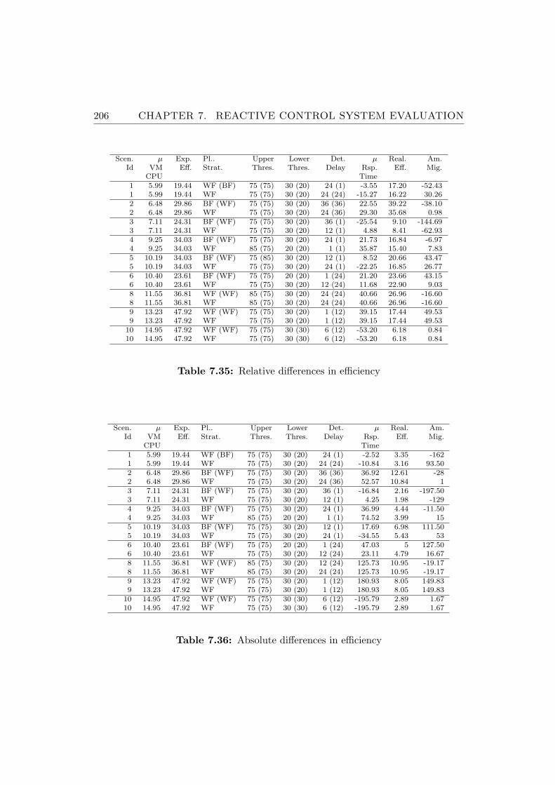
206 CHAPTER 7. REACTIVE CONTROL SYSTEM EVALUATION
Scen. µ Exp. Pl.. Upper Lower Det. µ Real. Am.Id VM Eff. Strat. Thres. Thres. Delay Rsp. Eff. Mig.
CPU Time1 5.99 19.44 WF (BF) 75 (75) 30 (20) 24 (1) -3.55 17.20 -52.431 5.99 19.44 WF 75 (75) 30 (20) 24 (24) -15.27 16.22 30.262 6.48 29.86 BF (WF) 75 (75) 30 (20) 36 (36) 22.55 39.22 -38.102 6.48 29.86 WF 75 (75) 30 (20) 24 (36) 29.30 35.68 0.983 7.11 24.31 BF (WF) 75 (75) 30 (20) 36 (1) -25.54 9.10 -144.693 7.11 24.31 WF 75 (75) 30 (20) 12 (1) 4.88 8.41 -62.934 9.25 34.03 BF (WF) 75 (75) 30 (20) 24 (1) 21.73 16.84 -6.974 9.25 34.03 WF 85 (75) 20 (20) 1 (1) 35.87 15.40 7.835 10.19 34.03 BF (WF) 75 (85) 30 (20) 12 (1) 8.52 20.66 43.475 10.19 34.03 WF 75 (75) 30 (20) 24 (1) -22.25 16.85 26.776 10.40 23.61 BF (WF) 75 (75) 20 (20) 1 (24) 21.20 23.66 43.156 10.40 23.61 WF 75 (75) 30 (20) 12 (24) 11.68 22.90 9.038 11.55 36.81 WF (WF) 85 (75) 30 (20) 24 (24) 40.66 26.96 -16.608 11.55 36.81 WF 85 (75) 30 (20) 24 (24) 40.66 26.96 -16.609 13.23 47.92 WF (WF) 75 (75) 30 (20) 1 (12) 39.15 17.44 49.539 13.23 47.92 WF 75 (75) 30 (20) 1 (12) 39.15 17.44 49.53
10 14.95 47.92 WF (WF) 75 (75) 30 (30) 6 (12) -53.20 6.18 0.8410 14.95 47.92 WF 75 (75) 30 (30) 6 (12) -53.20 6.18 0.84
Table 7.35: Relative differences in efficiency
Scen. µ Exp. Pl.. Upper Lower Det. µ Real. Am.Id VM Eff. Strat. Thres. Thres. Delay Rsp. Eff. Mig.
CPU Time1 5.99 19.44 WF (BF) 75 (75) 30 (20) 24 (1) -2.52 3.35 -1621 5.99 19.44 WF 75 (75) 30 (20) 24 (24) -10.84 3.16 93.502 6.48 29.86 BF (WF) 75 (75) 30 (20) 36 (36) 36.92 12.61 -282 6.48 29.86 WF 75 (75) 30 (20) 24 (36) 52.57 10.84 13 7.11 24.31 BF (WF) 75 (75) 30 (20) 36 (1) -16.84 2.16 -197.503 7.11 24.31 WF 75 (75) 30 (20) 12 (1) 4.25 1.98 -1294 9.25 34.03 BF (WF) 75 (75) 30 (20) 24 (1) 36.99 4.44 -11.504 9.25 34.03 WF 85 (75) 20 (20) 1 (1) 74.52 3.99 155 10.19 34.03 BF (WF) 75 (75) 30 (20) 12 (1) 17.69 6.98 111.505 10.19 34.03 WF 75 (75) 30 (20) 24 (1) -34.55 5.43 536 10.40 23.61 BF (WF) 75 (75) 20 (20) 1 (24) 47.03 5 127.506 10.40 23.61 WF 75 (75) 30 (20) 12 (24) 23.11 4.79 16.678 11.55 36.81 WF (WF) 85 (75) 30 (20) 12 (24) 125.73 10.95 -19.178 11.55 36.81 WF 85 (75) 30 (20) 24 (24) 125.73 10.95 -19.179 13.23 47.92 WF (WF) 75 (75) 30 (20) 1 (12) 180.93 8.05 149.839 13.23 47.92 WF 75 (75) 30 (20) 1 (12) 180.93 8.05 149.83
10 14.95 47.92 WF (WF) 75 (75) 30 (30) 6 (12) -195.79 2.89 1.6710 14.95 47.92 WF 75 (75) 30 (30) 6 (12) -195.79 2.89 1.67
Table 7.36: Absolute differences in efficiency
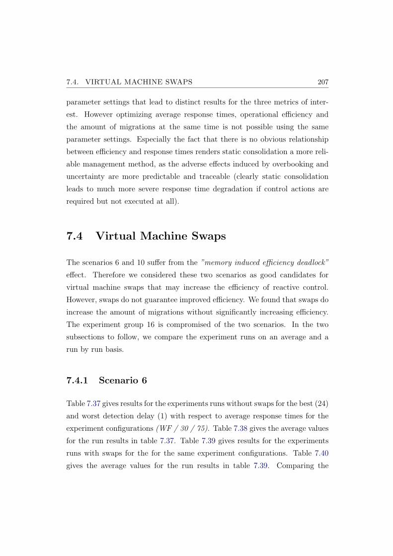
7.4. VIRTUAL MACHINE SWAPS 207
parameter settings that lead to distinct results for the three metrics of inter-
est. However optimizing average response times, operational efficiency and
the amount of migrations at the same time is not possible using the same
parameter settings. Especially the fact that there is no obvious relationship
between efficiency and response times renders static consolidation a more reli-
able management method, as the adverse effects induced by overbooking and
uncertainty are more predictable and traceable (clearly static consolidation
leads to much more severe response time degradation if control actions are
required but not executed at all).
7.4 Virtual Machine Swaps
The scenarios 6 and 10 suffer from the ”memory induced efficiency deadlock”
effect. Therefore we considered these two scenarios as good candidates for
virtual machine swaps that may increase the efficiency of reactive control.
However, swaps do not guarantee improved efficiency. We found that swaps do
increase the amount of migrations without significantly increasing efficiency.
The experiment group 16 is compromised of the two scenarios. In the two
subsections to follow, we compare the experiment runs on an average and a
run by run basis.
7.4.1 Scenario 6
Table 7.37 gives results for the experiments runs without swaps for the best (24)
and worst detection delay (1) with respect to average response times for the
experiment configurations (WF / 30 / 75). Table 7.38 gives the average values
for the run results in table 7.37. Table 7.39 gives results for the experiments
runs with swaps for the for the same experiment configurations. Table 7.40
gives the average values for the run results in table 7.39. Comparing the
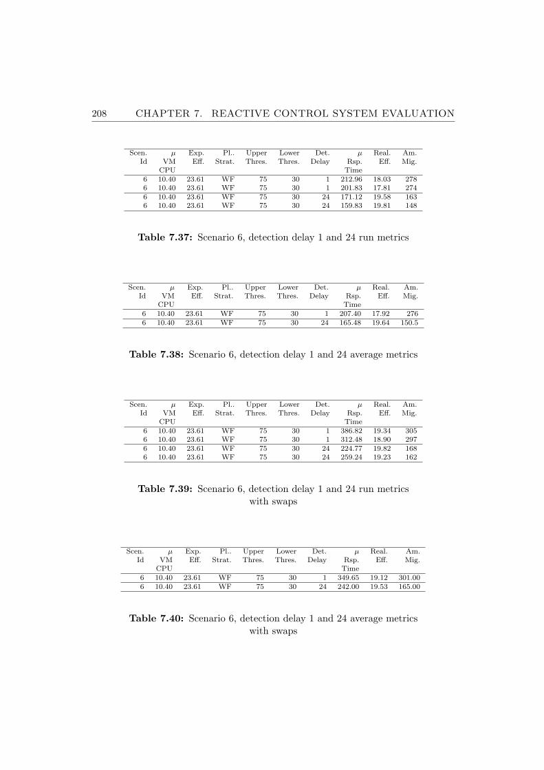
208 CHAPTER 7. REACTIVE CONTROL SYSTEM EVALUATION
Scen. µ Exp. Pl.. Upper Lower Det. µ Real. Am.Id VM Eff. Strat. Thres. Thres. Delay Rsp. Eff. Mig.
CPU Time6 10.40 23.61 WF 75 30 1 212.96 18.03 2786 10.40 23.61 WF 75 30 1 201.83 17.81 2746 10.40 23.61 WF 75 30 24 171.12 19.58 1636 10.40 23.61 WF 75 30 24 159.83 19.81 148
Table 7.37: Scenario 6, detection delay 1 and 24 run metrics
Scen. µ Exp. Pl.. Upper Lower Det. µ Real. Am.Id VM Eff. Strat. Thres. Thres. Delay Rsp. Eff. Mig.
CPU Time6 10.40 23.61 WF 75 30 1 207.40 17.92 2766 10.40 23.61 WF 75 30 24 165.48 19.64 150.5
Table 7.38: Scenario 6, detection delay 1 and 24 average metrics
Scen. µ Exp. Pl.. Upper Lower Det. µ Real. Am.Id VM Eff. Strat. Thres. Thres. Delay Rsp. Eff. Mig.
CPU Time6 10.40 23.61 WF 75 30 1 386.82 19.34 3056 10.40 23.61 WF 75 30 1 312.48 18.90 2976 10.40 23.61 WF 75 30 24 224.77 19.82 1686 10.40 23.61 WF 75 30 24 259.24 19.23 162
Table 7.39: Scenario 6, detection delay 1 and 24 run metricswith swaps
Scen. µ Exp. Pl.. Upper Lower Det. µ Real. Am.Id VM Eff. Strat. Thres. Thres. Delay Rsp. Eff. Mig.
CPU Time6 10.40 23.61 WF 75 30 1 349.65 19.12 301.006 10.40 23.61 WF 75 30 24 242.00 19.53 165.00
Table 7.40: Scenario 6, detection delay 1 and 24 average metricswith swaps
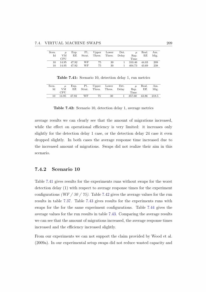
7.4. VIRTUAL MACHINE SWAPS 209
Scen. µ Exp. Pl.. Upper Lower Det. µ Real. Am.Id VM Eff. Strat. Thres. Thres. Delay Rsp. Eff. Mig.
CPU Time10 14.95 47.92 WF 75 30 1 310.46 44.03 20910 14.95 47.92 WF 75 30 1 404.73 43.69 238
Table 7.41: Scenario 10, detection delay 1, run metrics
Scen. µ Exp. Pl.. Upper Lower Det. µ Real. Am.Id VM Eff. Strat. Thres. Thres. Delay Rsp. Eff. Mig.
CPU Time10 14.95 47.92 WF 75 30 1 357.60 43.86 218.5
Table 7.42: Scenario 10, detection delay 1, average metrics
average results we can clearly see that the amount of migrations increased,
while the effect on operational efficiency is very limited: it increases only
slightly for the detection delay 1 case, or the detection delay 24 case it even
dropped slightly. In both cases the average response time increased due to
the increased amount of migrations. Swaps did not realize their aim in this
scenario.
7.4.2 Scenario 10
Table 7.41 gives results for the experiments runs without swaps for the worst
detection delay (1) with respect to average response times for the experiment
configurations (WF / 30 / 75). Table 7.42 gives the average values for the run
results in table 7.37. Table 7.43 gives results for the experiments runs with
swaps for the for the same experiment configurations. Table 7.44 gives the
average values for the run results in table 7.43. Comparing the average results
we can see that the amount of migrations increased, the average response times
increased and the efficiency increased slightly.
From our experiments we can not support the claim provided by Wood et al.
(2009a). In our experimental setup swaps did not reduce wasted capacity and
210 CHAPTER 7. REACTIVE CONTROL SYSTEM EVALUATION
Scen. µ Exp. Pl.. Upper Lower Det. µ Real. Am.Id VM Eff. Strat. Thres. Thres. Delay Rsp. Eff. Mig.
CPU Time10 14.95 47.92 WF 75 30 1 485.38 45.19 25610 14.95 47.92 WF 75 30 1 410.82 44.68 230
Table 7.43: Scenario 10, detection delay 1, run metrics withswaps
Scen. µ Exp. Pl.. Upper Lower Det. µ Real. Am.Id VM Eff. Strat. Thres. Thres. Delay Rsp. Eff. Mig.
CPU Time10 14.95 47.92 WF 75 30 1 448.10 44.94 238
Table 7.44: Scenario 10, detection delay 1, average metrics withswaps
improved load balancing to a significant extend. On the contrary, swaps lead
to increased numbers of live migrations which leads to higher overheads and
application performance degradation. As the selected test scenarios exposed
allocation problems that we expected to be solved by swaps, we did not extend
our study to other scenarios. Our insights do not justify the usage of swaps.
7.5 Causes for Excessive Amounts of Migra-
tions
As we have shown in the preceding sections, the amount of migrations executed
by the reactive control system is often found to be much higher than the
expected amount of migrations. This behavior is due to several reasons:
• Aggressiveness of threshold values: If the operational corridor, induced
by the upper and lower thresholds is too narrow, the control system
is operating in a too aggressive mode. However, choosing the corridor
too widely either leads to lost efficiency or to application performance

7.5. CAUSES FOR EXCESSIVE AMOUNTS OF MIGRATIONS 211
degradation: too high upper thresholds lead to severe overloads during
migration execution, too low high values require much more physical
servers. Too low lower threshold values lead to lost efficiency, too high
lower threshold values lead to oscillations as we move high demand vir-
tual machines first, then smaller ones.
• Non effectiveness migrations: It is unknown to the controller whether the
evacuation of a server can be realized or not. The controller does do con-
sider the current system state to estimate whether the virtual machines
of one or several under-loaded servers can be consolidated on the re-
maining physical servers? If it is not possible to fully evacuate a physical
server, no migrations should be triggered at all. We have tested a tenta-
tive version of the controller that uses a randomized first fit placement
algorithm to determine whether the amount of required physical servers
can be reduced. In case it is possible an evacuation enabled, if not, no
migration is issued from under-loaded physical servers. We executed 4
experiment runs, which lead to a reduction of migrations of about 3.28%
on average. During times of high resource demands almost no reduction
could be observed as well as no impact on response times. The tentative
controller prevented unnecessary migrations during times of declining
demands, delaying the shrinkage of the set of required physical servers.
Therefore almost no impact on response times could be observed. The
tentative controller could not deliver substantial improvements.
• Consolidation overheads: Non-additive resource demands, especially for
virtual machines with memory intensive workloads lead to bad placement
decisions. Therefore the worst fit placement strategy performs better
as it allows for more headroom for uncertainty and compensates bad
demand estimations.
• Placement decisions: Ad-hoc placement decisions can not be expected to
find an optimal allocation and may not even realize them as (multiway)
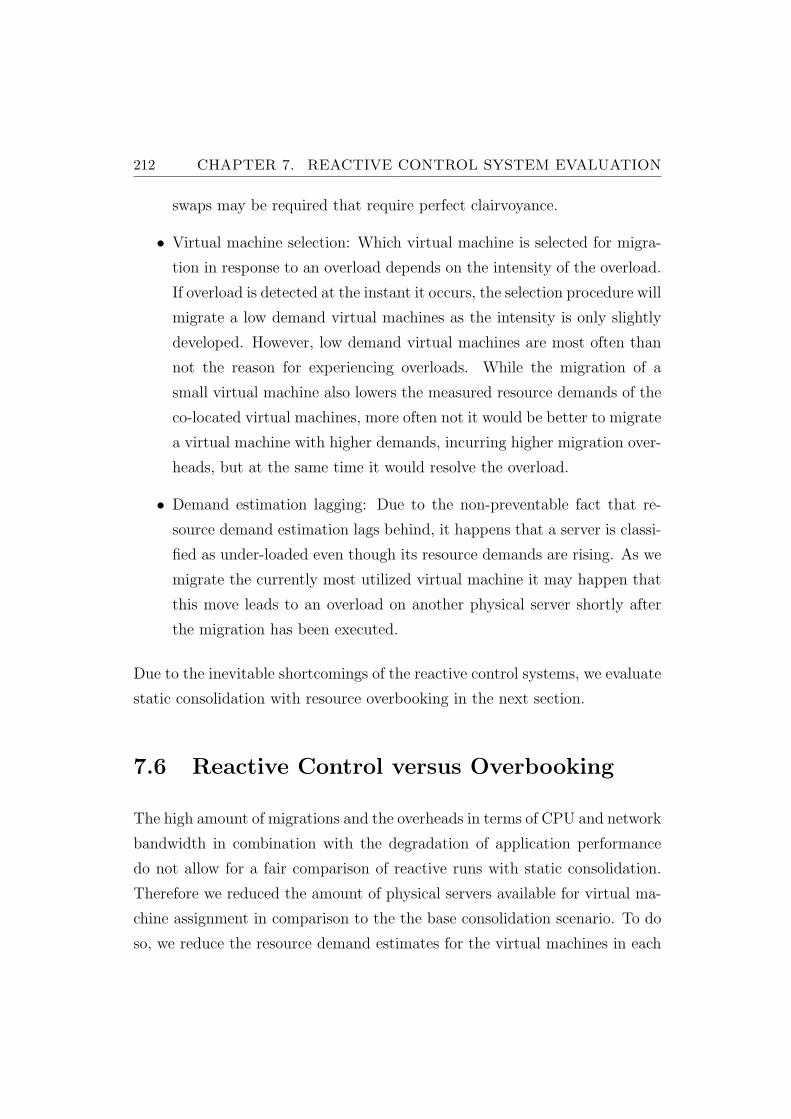
212 CHAPTER 7. REACTIVE CONTROL SYSTEM EVALUATION
swaps may be required that require perfect clairvoyance.
• Virtual machine selection: Which virtual machine is selected for migra-
tion in response to an overload depends on the intensity of the overload.
If overload is detected at the instant it occurs, the selection procedure will
migrate a low demand virtual machines as the intensity is only slightly
developed. However, low demand virtual machines are most often than
not the reason for experiencing overloads. While the migration of a
small virtual machine also lowers the measured resource demands of the
co-located virtual machines, more often not it would be better to migrate
a virtual machine with higher demands, incurring higher migration over-
heads, but at the same time it would resolve the overload.
• Demand estimation lagging: Due to the non-preventable fact that re-
source demand estimation lags behind, it happens that a server is classi-
fied as under-loaded even though its resource demands are rising. As we
migrate the currently most utilized virtual machine it may happen that
this move leads to an overload on another physical server shortly after
the migration has been executed.
Due to the inevitable shortcomings of the reactive control systems, we evaluate
static consolidation with resource overbooking in the next section.
7.6 Reactive Control versus Overbooking
The high amount of migrations and the overheads in terms of CPU and network
bandwidth in combination with the degradation of application performance
do not allow for a fair comparison of reactive runs with static consolidation.
Therefore we reduced the amount of physical servers available for virtual ma-
chine assignment in comparison to the the base consolidation scenario. To do
so, we reduce the resource demand estimates for the virtual machines in each
7.6. REACTIVE CONTROL VERSUS OVERBOOKING 213
time interval iteratively by 0.5% and calculated a new assignment until we were
able to reduced the number or required physical servers by one. This leads to a
systematic underestimation of the resource demands of virtual machines and a
reduction in required physical servers, which is often referred to as overbooking
(Urgaonkar et al., 2009). In the following we give an average comparison on
the response times and efficiency achieved by overbooking resources as finding
the right control parameters for a reactive control system is dependent on the
overall workload characteristics and other factors. Therefore we assume an
average case by calculating the mean response time and mean efficiency over
all reactive control runs executed in the experiment groups 1 - 11 and compare,
on a scenario basis, the delivered efficiency and response times with the same
metrics achieved by overbooking by a given percentage. We compare, on a
scenario basis, the delivered efficiency and response times with the efficiency
achieved by overbooking by 16.66, 33.33 and 50.00% which relates to reducing
the amount of physical servers from 6 to 5, 4 and 3. Please note that we do
not reduce the amount of servers to 3 for all scenarios as this would not have
been possible for scenarios with relatively large amounts of virtual machines:
The minimum number of servers is restricted by main memory demands.
As it is hard to determine the best control system parameters for any given
workload scenario, the mean case, that is the average of the mean response
times and efficiency over all reactive control runs is the fairest comparison ba-
sis for overbooking. As can be seen in figure 7.11 and table 7.45, overbooking
is even more competitive, especially for scenarios with large virtual machine
capacities. Overbooking by 33.33% outperforms or comes close to dynamic
workload management in terms of operational efficiency. For scenarios with
large virtual machines, the response times are even better, while for the re-
maining scenarios, the degradations are moderate. Overbooking by 50.00%
might be acceptable, as the response time penalty for very large scenarios is
about 300%, but delivers almost 5% better operational efficiency.
According to the average case comparison, resource overbooking is a viable
214 CHAPTER 7. REACTIVE CONTROL SYSTEM EVALUATION
6 8 10 12 14
−10
00−
500
050
0
Mean Case
Res
pons
e T
ime
(%)
●
●
●
● ● ●
●
●
●
●
16.66 %33.33 %50.00 %
6 8 10 12 14
−20
020
40
Mean VM CPU Demand
Effi
cien
cy (
%)
●
●
●●
●
●
●
●●
●
16.66 %33.33 %50.00 %
Figure 7.11: Overbooking versus mean case
Scenario 1 2 3 4 5 6 8 9 1016.66 % µ Rsp. -31.11 130.24 -72.64 124.75 112.18 136.83 134.05 242.19 308.8616.66 % Eff. 1.50 11.08 6.08 7.95 13.60 2.64 18.72 27.08 28.8733.33 % µ Rsp. -471.46 57.90 -323.00 -80.97 -84.84 -83.11 65.42 132.07 46.4733.33 % Eff. -15.17 -5.59 -10.59 -8.72 -3.07 -14.03 2.05 10.41 12.2050.00 % µ Rsp. 0.00 0.00 0.00 0.00 -682.75 -788.31 -574.75 -293.29 -332.0750.00 % Eff. -30.70 -22.26 -27.26 -31.84 -25.39 -19.74 -14.62 -6.26 -4.47µ CPU VM 5.99 6.48 7.11 9.25 10.19 10.40 11.55 13.23 14.95
Table 7.45: Overbooking versus mean case, summary statistics
7.6. REACTIVE CONTROL VERSUS OVERBOOKING 215
alternative to dynamic workload management as it is afflicted with overheads
and response time degradation. In appendix D, we provide an analysis of
the expected, minimum and maximum cases. The mean case reveals that
overbooking of a percentage between 16.66% and 33.33% is balancing out the
response time penalties with operational efficiency. In a real world consoli-
dation scenario, we are give much more servers. There, it is perceivable to
find an overbooking level that renders overbooking as efficient as reactive con-
trol and delivers about the same average response times. Even the minimum
case suggests that moderate overbooking of about 16.66% is advisable for data
center operators for all types of scenarios. Our results indicate that resource
overbooking in combination with very careful, damped reactive control system
design is a very promising combination to balance out response time service
levels with operational efficiency.
Chapter 8
Conclusion
The main scientific contribution of the presented work is the experimental
evaluation of a reactive control system for virtualized data centres and a com-
parison with static server consolidation and resource overbooking for enterprise
application. We explicitly aimed at studying typical instantiations of normal
resource demand behavior of virtual machines to gain unbiased and represen-
tative insights. The comparison revealed that dynamic management is su-
perior to conservative server consolidation when assuming CPU as the main
bottleneck resource. However, more aggressive server consolidation plans incur
only short periods of overloads with acceptable shortage intensities and come
close to reactive control methods in terms of operational efficiency and deliv-
ered application performance. Due to the real-time requirements for reactive
control systems and high levels of uncertainty for future resource demands,
more often than not ad-hoc virtual machine placement decisions lead to much
more virtual machine live migrations than required. Migrations have a sig-
nificant impact on application response times even for benchmark scenarios
with moderate average workload levels. We compared the results of more
aggressive consolidation planning and showed that it is feasible to overbook
CPU resources in a way that renders static server consolidation preferable
216
217
over dynamic workload management. Reactive control is indeed able to real-
ize potential efficiency gains in comparison to static consolidation but is not
able to deliver comparable levels of application response times. However, the
optimal parameterization of reactive control systems is heavily dependent on
the characteristics of the data centre wide workload and parameter settings
are often hard to tune towards the desired operational goal metric. An equi-
librium between delivered response times and operational efficiency is only
achievable by incurring significant overheads on the infrastructure. Therefore,
static consolidation and resource overbooking turn out to be preferable over
dynamic workload management as the combination of unavoidable prediction
and detection delays renders heavy weight control actions more often than not
ineffective.
We have to mention that our results are, to a certain extend, bound to the sys-
tem configuration of our testbed. Several realization choices and the hardware
setup influence these results, especially the effect of migration and consolida-
tion overheads can be expected to be less severe for higher quality hardware
equipment used in today’s enterprise data centres. It is also perceivable that
reactive control can be improved upon by incorporating online consolidation
overhead estimation procedures. Nevertheless, we believe that our main claim
holds for other setups as well: Aggressive, static sever consolidation is com-
petitive with any dynamic control approach, even if dynamic control unfolds
its efficiency potential to the fullest extend.
Our insights may be used to improve existing control systems that combine
pre-computed virtual machine to physical server assignments with carefully
designed anomaly detection and conditioning strategies. By combining aggres-
sive overbooking methods with reactive anomaly handling and predetermined
consolidation schedules, better results may be obtained for dynamic workload
management. Furthermore, adjusting the detection delay and threshold set-
tings according to the relative workload intensity may allow for less migrations
overheads.
218 CHAPTER 8. CONCLUSION
As we have given the first extensive study on reactive control systems in a real
world testbed, we have brought up several issues that have not been addressed
by other scientific studies. Partially, our results are in contradiction and cast a
different light on the results existing studies have drawn out. This is due to the
fact that most existing studies are based on computer simulations and assump-
tions about migration overheads that do not hold true in real infrastructures.
In contrast to studies that have been executed in real testbeds, we provide a
more rigorous and transparent evaluation of strengths and weaknesses of reac-
tive control systems and give in depth results that support design choices and
system implementation rationales.
Appendix A
Consolidation Overheads
In table A.1 we provide results for experiments executed with two virtual ma-
chines serving non-equal amounts of virtual users. Each row in the table is
marked with a type. Type 1 marks the measured resource demands and gives
the consolidation overhead in percent compared type 2, which gives the re-
source demand expected under additivity. The overheads deviate from the
symmetric case. For 40 virtual users, the overheads are slightly less, but we
have to note that for most other cases, the asymmetric overheads are higher.
One reason for this observation is that high demand levels for a single vir-
tual machine lead to a strong dependence on the effectiveness of hardware
caches. The displacement of memory pages in the caches, caused by low de-
mand co-located virtual machines leads to higher cache miss rates for all vir-
tual machines, requiring more cycles per instruction, and hence leads to higher
processor utilization.
Table A.2 lists the results for experiments executed with four virtual machines
serving non-equal amounts of virtual users. For four virtual machines, sim-
ilar observations can be derived as for the two virtual machine asymmetric
workload experiments. If there are highly loaded virtual machines competing
for hardware resources with lightly loaded virtual machines, the highly loaded
219
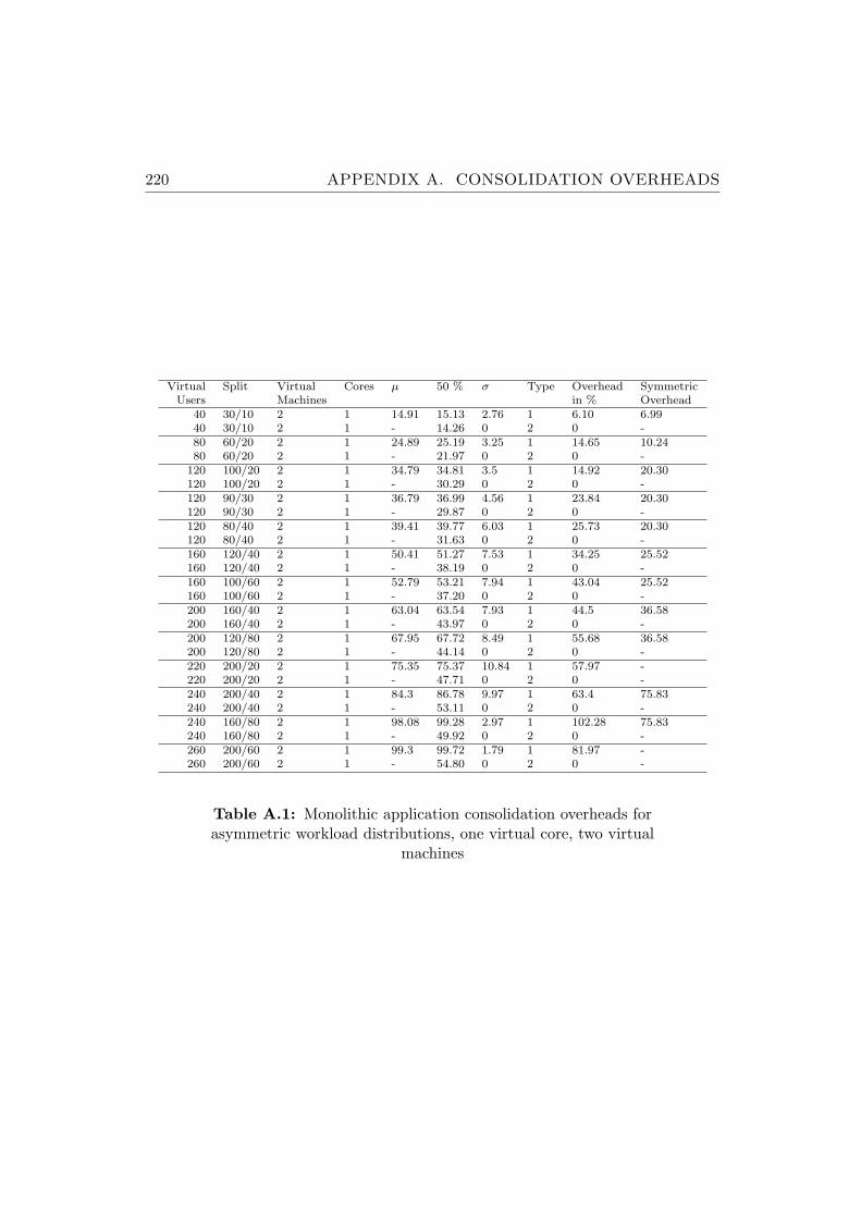
220 APPENDIX A. CONSOLIDATION OVERHEADS
Virtual Split Virtual Cores µ 50 % σ Type Overhead SymmetricUsers Machines in % Overhead
40 30/10 2 1 14.91 15.13 2.76 1 6.10 6.9940 30/10 2 1 - 14.26 0 2 0 -80 60/20 2 1 24.89 25.19 3.25 1 14.65 10.2480 60/20 2 1 - 21.97 0 2 0 -
120 100/20 2 1 34.79 34.81 3.5 1 14.92 20.30120 100/20 2 1 - 30.29 0 2 0 -120 90/30 2 1 36.79 36.99 4.56 1 23.84 20.30120 90/30 2 1 - 29.87 0 2 0 -120 80/40 2 1 39.41 39.77 6.03 1 25.73 20.30120 80/40 2 1 - 31.63 0 2 0 -160 120/40 2 1 50.41 51.27 7.53 1 34.25 25.52160 120/40 2 1 - 38.19 0 2 0 -160 100/60 2 1 52.79 53.21 7.94 1 43.04 25.52160 100/60 2 1 - 37.20 0 2 0 -200 160/40 2 1 63.04 63.54 7.93 1 44.5 36.58200 160/40 2 1 - 43.97 0 2 0 -200 120/80 2 1 67.95 67.72 8.49 1 55.68 36.58200 120/80 2 1 - 44.14 0 2 0 -220 200/20 2 1 75.35 75.37 10.84 1 57.97 -220 200/20 2 1 - 47.71 0 2 0 -240 200/40 2 1 84.3 86.78 9.97 1 63.4 75.83240 200/40 2 1 - 53.11 0 2 0 -240 160/80 2 1 98.08 99.28 2.97 1 102.28 75.83240 160/80 2 1 - 49.92 0 2 0 -260 200/60 2 1 99.3 99.72 1.79 1 81.97 -260 200/60 2 1 - 54.80 0 2 0 -
Table A.1: Monolithic application consolidation overheads forasymmetric workload distributions, one virtual core, two virtual
machines
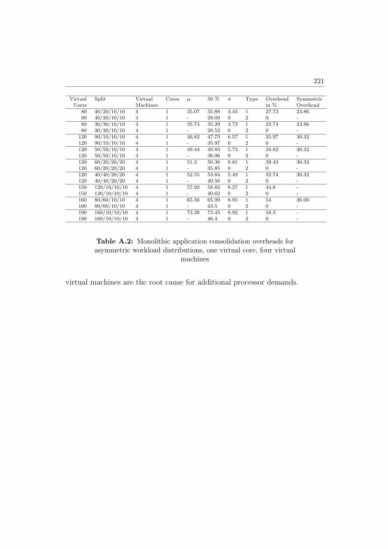
221
Virtual Split Virtual Cores µ 50 % σ Type Overhead SymmetricUsers Machines in % Overhead
80 40/20/10/10 4 1 35.07 35.88 4.43 1 27.73 23.8680 40/20/10/10 4 1 - 28.09 0 2 0 -80 30/30/10/10 4 1 35.74 35.29 4.73 1 23.74 23.8680 30/30/10/10 4 1 - 28.52 0 2 0 -
120 90/10/10/10 4 1 46.82 47.73 6.57 1 35.97 30.32120 90/10/10/10 4 1 - 35.97 0 2 0 -120 50/50/10/10 4 1 49.44 49.83 5.73 1 34.82 30.32120 50/50/10/10 4 1 - 36.96 0 2 0 -120 60/20/20/20 4 1 51.2 50.38 9.81 1 39.43 30.32120 60/20/20/20 4 1 - 35.85 0 2 0 -120 40/40/20/20 4 1 52.55 53.84 5.49 1 32.74 30.32120 40/40/20/20 4 1 - 40.56 0 2 0 -150 120/10/10/10 4 1 57.92 58.82 8.27 1 44.8 -150 120/10/10/10 4 1 - 40.62 0 2 0 -160 80/60/10/10 4 1 65.56 65.99 8.85 1 54 36.00160 80/60/10/10 4 1 - 43.5 0 2 0 -190 160/10/10/10 4 1 73.39 73.45 8.92 1 58.3 -190 160/10/10/10 4 1 - 46.4 0 2 0 -
Table A.2: Monolithic application consolidation overheads forasymmetric workload distributions, one virtual core, four virtual
machines
virtual machines are the root cause for additional processor demands.
Appendix B
Consolation Overhead
Estimation
B.1 Database Consolidation Overheads
As the consolidation overheads can be accounted to the main memory access
behavior of the applications running in a virtual machine, we conducted the
consolidation overhead experiments for databases as well. Figure B.1 gives
the CPU demands for a single database virtual machine running in isolation
on a physical server. Figure B.2 visualizes the consolidation overheads for two
database servers. As we expected, the relative overheads (for comparable CPU
demand levels) are by far smaller than those measured for the monolithic appli-
cation configuration. The same observation applies to four virtual machines
(figure B.3) and eight virtual machines (figure B.4). The effect is due to the
less main memory requirements for database servers than for the monolithic
application configuration and much less dependence on cache performance.
I/O performance is more influential for this type of workload. Figure B.5 gives
the overhead estimation function for database virtual machines. Its shape is
similar to the shape of the monolithic application configuration function.
222
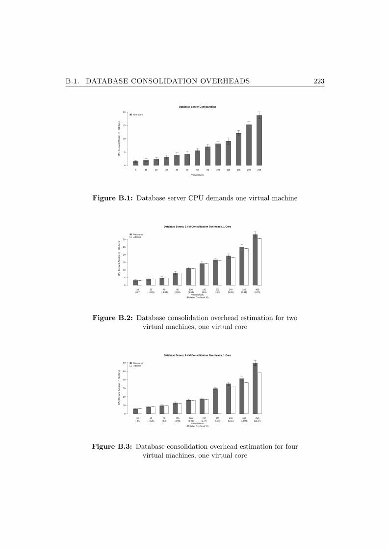
B.1. DATABASE CONSOLIDATION OVERHEADS 223
5 10 20 30 40 50 60 80 100 120 160 200 240
Database Server Configuration
Virtual Users
CP
U D
eman
d (M
edia
n +
/− S
td.D
ev.)
0
5
10
15
20One Core
Figure B.1: Database server CPU demands one virtual machine
10 20 40 80 120 160 200 240 320 400
Database Server, 2 VM Consolidation Overheads, 1 Core
(Relative Overhead %)Virtual Users
CP
U D
eman
d (M
edia
n +
/− S
td.D
ev.)
0
5
10
15
20
25
30
MeasuredAdditive
(4.67) (−0.25) (−3.83) (0.51) (1.64) (1.5) (1.73) (5.06) (4.31) (8.79)
Figure B.2: Database consolidation overhead estimation for twovirtual machines, one virtual core
20 40 80 120 160 200 320 400 480 640
Database Server, 4 VM Consolidation Overheads, 1 Core
(Relative Overhead %)Virtual Users
CP
U D
eman
d (M
edia
n +
/− S
td.D
ev.)
0
10
20
30
40
50
60 MeasuredAdditive
(−2.5) (−0.25) (3.3) (2.02) (2.42) (3.74) (6.33) (8.55) (13.83) (23.67)
Figure B.3: Database consolidation overhead estimation for fourvirtual machines, one virtual core
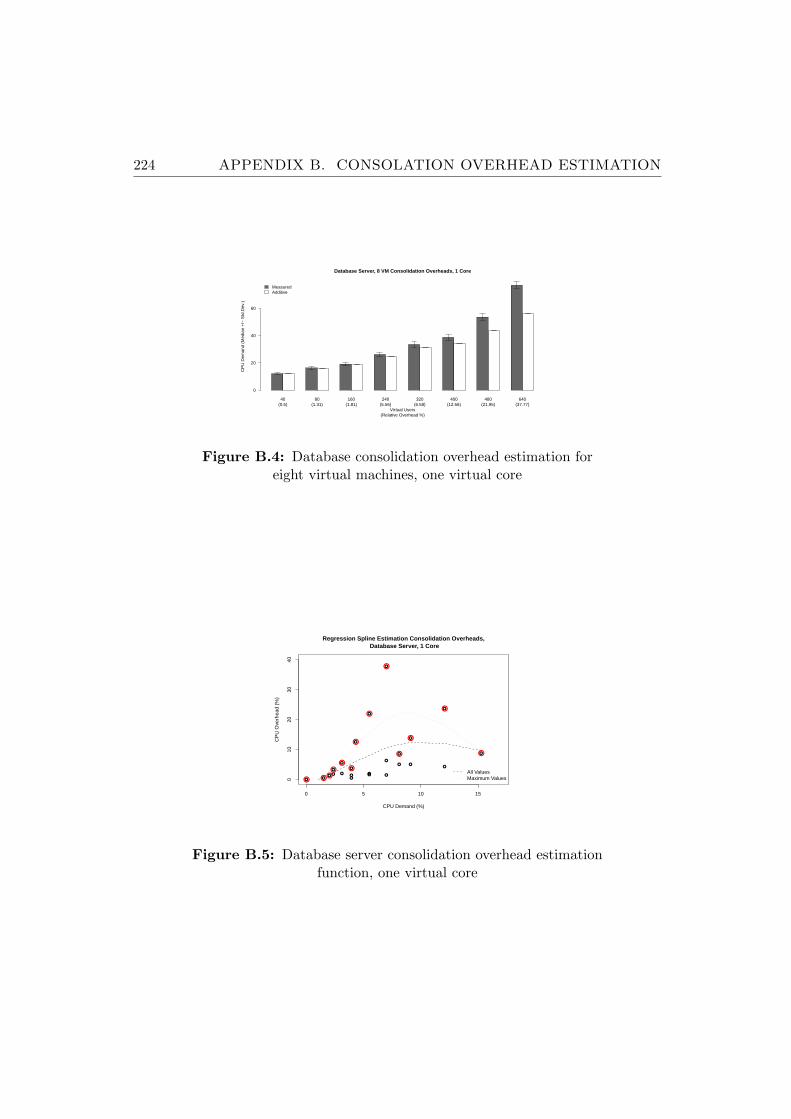
224 APPENDIX B. CONSOLATION OVERHEAD ESTIMATION
40 80 160 240 320 400 480 640
Database Server, 8 VM Consolidation Overheads, 1 Core
(Relative Overhead %)Virtual Users
CP
U D
eman
d (M
edia
n +
/− S
td.D
ev.)
0
20
40
60
MeasuredAdditive
(0.5) (1.31) (1.81) (5.56) (6.58) (12.56) (21.95) (37.77)
Figure B.4: Database consolidation overhead estimation foreight virtual machines, one virtual core
● ●● ●
● ●●
●
●●
●
●
●
●
●
●● ●
●
●
●
●
●●
0 5 10 15
010
2030
40
Regression Spline Estimation Consolidation Overheads, Database Server, 1 Core
CPU Demand (%)
CP
U O
verh
ead
(%)
● ●●●
●●
●
●
●
●
●
●
●
All ValuesMaximum Values
Figure B.5: Database server consolidation overhead estimationfunction, one virtual core
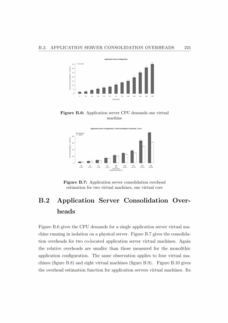
B.2. APPLICATION SERVER CONSOLIDATION OVERHEADS 225
5 10 20 30 40 50 60 80 100 120 160 200 240
Application Server Configuration
Virtual Users
Pro
cess
or D
eman
d (M
edia
n +
/− S
td.D
ev.)
0
5
10
15
20
25
30
35 One Core
Figure B.6: Application server CPU demands one virtualmachine
10 20 40 80 120 160 200 320 400
Application Server Configuration, 2 VM Consolidation Overheads, 1 Core
(Relative Overhead %)Virtual Users
CP
U D
eman
d (M
edia
n +
/− S
td.D
ev.)
0
20
40
60
80
MeasuredAdditive
(1.06) (1.97) (1.31) (5.33) (8.4) (12.36) (22.16) (32.72) (46.66)
Figure B.7: Application server consolidation overheadestimation for two virtual machines, one virtual core
B.2 Application Server Consolidation Over-
heads
Figure B.6 gives the CPU demands for a single application server virtual ma-
chine running in isolation on a physical server. Figure B.7 gives the consolida-
tion overheads for two co-located application server virtual machines. Again
the relative overheads are smaller than those measured for the monolithic
application configuration. The same observation applies to four virtual ma-
chines (figure B.8) and eight virtual machines (figure B.9). Figure B.10 gives
the overhead estimation function for application servers virtual machines. Its
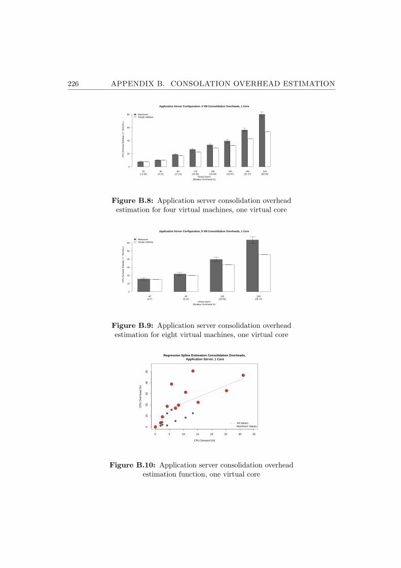
226 APPENDIX B. CONSOLATION OVERHEAD ESTIMATION
20 40 80 120 160 200 240 320
Application Server Configuration, 4 VM Consolidation Overheads, 1 Core
(Relative Overhead %)Virtual Users
CP
U D
eman
d (M
edia
n +
/− S
td.D
ev.)
0
20
40
60
80 MeasuredSimple Additive
(−0.65) (4.22) (12.23) (15.45) (16.94) (19.67) (31.27) (50.56)
Figure B.8: Application server consolidation overheadestimation for four virtual machines, one virtual core
40 80 160 240
Application Server Configuration, 8 VM Consolidation Overheads, 1 Core
(Relative Overhead %)Virtual Users
CP
U D
eman
d (M
edia
n +
/− S
td.D
ev.)
0
10
20
30
40
50
60
MeasuredSimple Additive
(3.7) (9.14) (18.59) (38.72)
Figure B.9: Application server consolidation overheadestimation for eight virtual machines, one virtual core
●●
● ●
●
●
●
●
●
●
●
●
●●
●
●
●
●
●
●
●
0 5 10 15 20 25 30 35
010
2030
4050
Regression Spline Estimation Consolidation Overheads, Application Server, 1 Core
CPU Demand (%)
CP
U O
verh
ead
(%)
●
●
●
●
●
●●
●
●
●
●
●
All ValuesMaximum Values
Figure B.10: Application server consolidation overheadestimation function, one virtual core

B.2. APPLICATION SERVER CONSOLIDATION OVERHEADS 227
shape is similar to the shape of the monolithic application configuration and
the database server function. However, the overheads are more pronounced for
application server than for database server virtual machines. The observation
can again be explained by higher dependencies of main memory access and
usage patterns of the application server workload.
Appendix C
Resource Demand Estimation
C.1 Consolidation Run Data Results
Figure C.1 presents the prediction results for six steps ahead forecasts (30
seconds real time). The best smoothers are the SMA6 an ATM6, but are
only slightly better than the EMA6 smoother. As the differences between the
smoothers become less significant, the differences between the smoother and
the forecasting models also decrease further as table C.1 reveals.
228
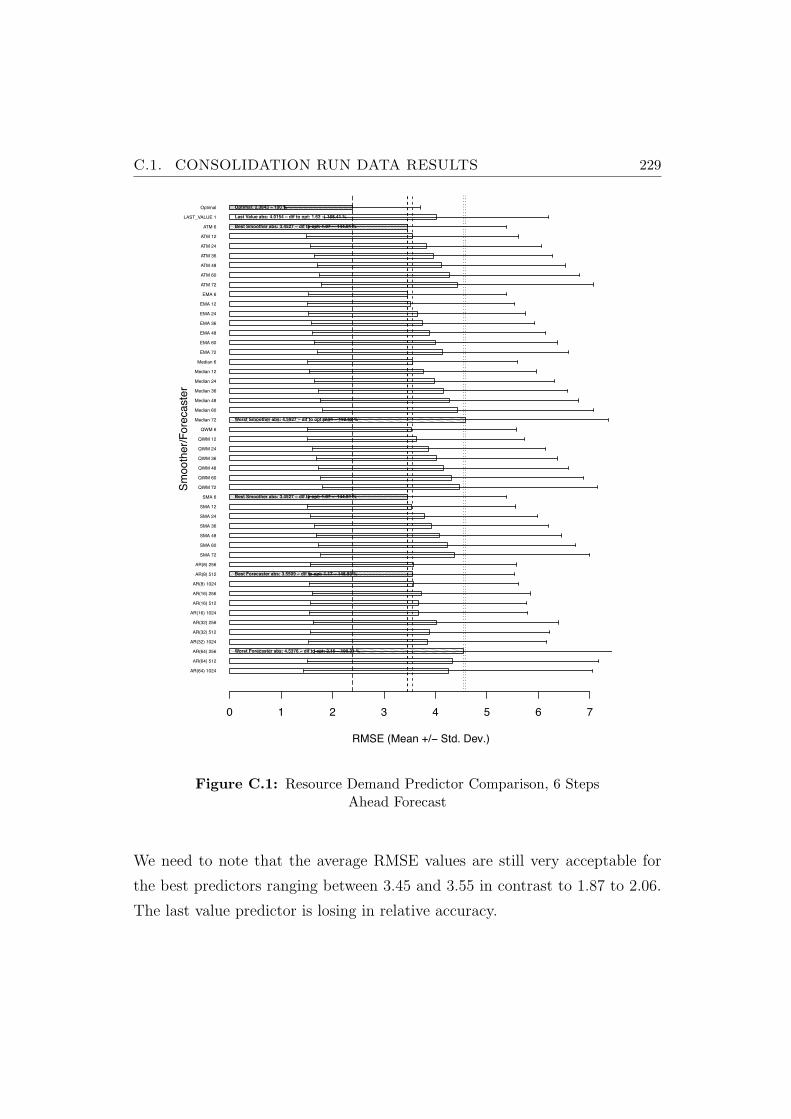
C.1. CONSOLIDATION RUN DATA RESULTS 229
AR(64) 1024
AR(64) 512
AR(64) 256
AR(32) 1024
AR(32) 512
AR(32) 256
AR(16) 1024
AR(16) 512
AR(16) 256
AR(8) 1024
AR(8) 512
AR(8) 256
SMA 72
SMA 60
SMA 48
SMA 36
SMA 24
SMA 12
SMA 6
QWM 72
QWM 60
QWM 48
QWM 36
QWM 24
QWM 12
QWM 6
Median 72
Median 60
Median 48
Median 36
Median 24
Median 12
Median 6
EMA 72
EMA 60
EMA 48
EMA 36
EMA 24
EMA 12
EMA 6
ATM 72
ATM 60
ATM 48
ATM 36
ATM 24
ATM 12
ATM 6
LAST_VALUE 1
Optimal
Optimal Forecaster vs. Smoother/Forecaster for Lookahead 6
RMSE (Mean +/! Std. Dev.)
Sm
ooth
er/
Fore
caste
r
0 1 2 3 4 5 6 7
Optimal: 2.3843 ! 100 %
Last Value abs: 4.0154 ! dif to opt: 1.63 ! 168.41 %
Best Smoother abs: 3.4527 ! dif to opt: 1.07 ! 144.81 %
Best Smoother abs: 3.4527 ! dif to opt: 1.07 ! 144.81 %
Worst Smoother abs: 4.5927 ! dif to opt: 2.21 ! 192.62 %
Best Forecaster abs: 3.5509 ! dif to opt: 1.17 ! 148.93 %
Worst Forecaster abs: 4.5376 ! dif to opt: 2.15 ! 190.31 %
Figure C.1: Resource Demand Predictor Comparison, 6 StepsAhead Forecast
We need to note that the average RMSE values are still very acceptable for
the best predictors ranging between 3.45 and 3.55 in contrast to 1.87 to 2.06.
The last value predictor is losing in relative accuracy.
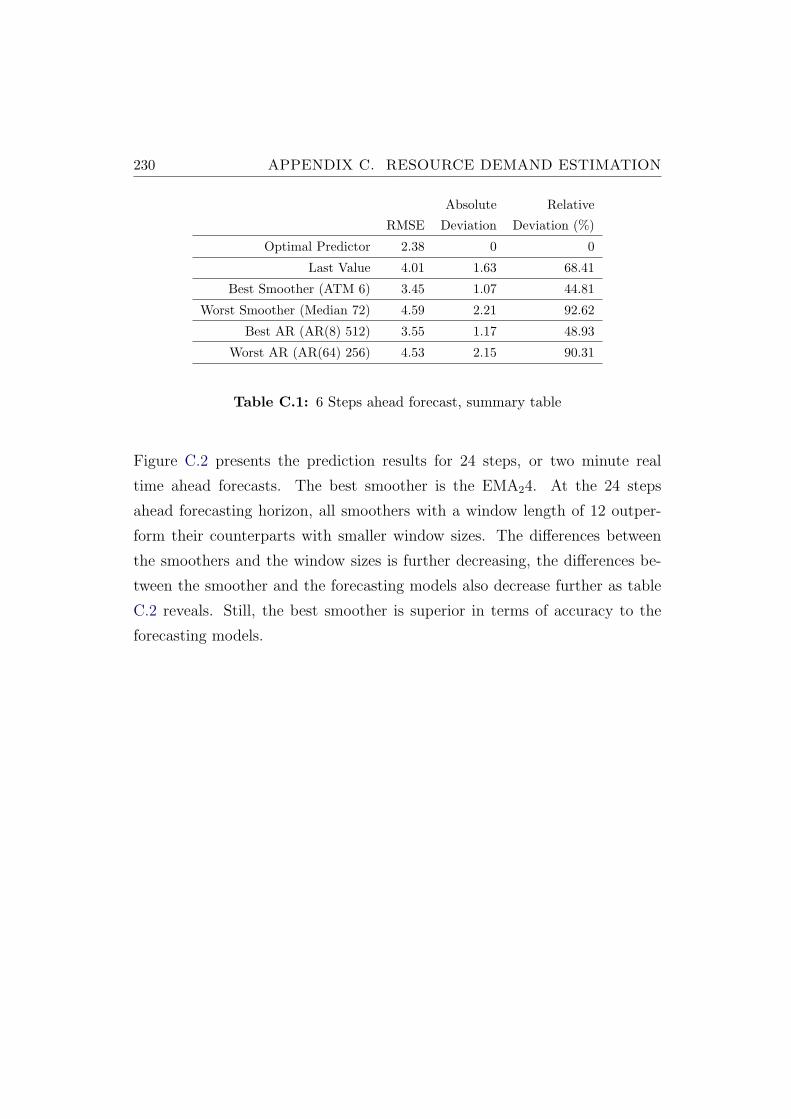
230 APPENDIX C. RESOURCE DEMAND ESTIMATION
Absolute Relative
RMSE Deviation Deviation (%)
Optimal Predictor 2.38 0 0
Last Value 4.01 1.63 68.41
Best Smoother (ATM 6) 3.45 1.07 44.81
Worst Smoother (Median 72) 4.59 2.21 92.62
Best AR (AR(8) 512) 3.55 1.17 48.93
Worst AR (AR(64) 256) 4.53 2.15 90.31
Table C.1: 6 Steps ahead forecast, summary table
Figure C.2 presents the prediction results for 24 steps, or two minute real
time ahead forecasts. The best smoother is the EMA24. At the 24 steps
ahead forecasting horizon, all smoothers with a window length of 12 outper-
form their counterparts with smaller window sizes. The differences between
the smoothers and the window sizes is further decreasing, the differences be-
tween the smoother and the forecasting models also decrease further as table
C.2 reveals. Still, the best smoother is superior in terms of accuracy to the
forecasting models.
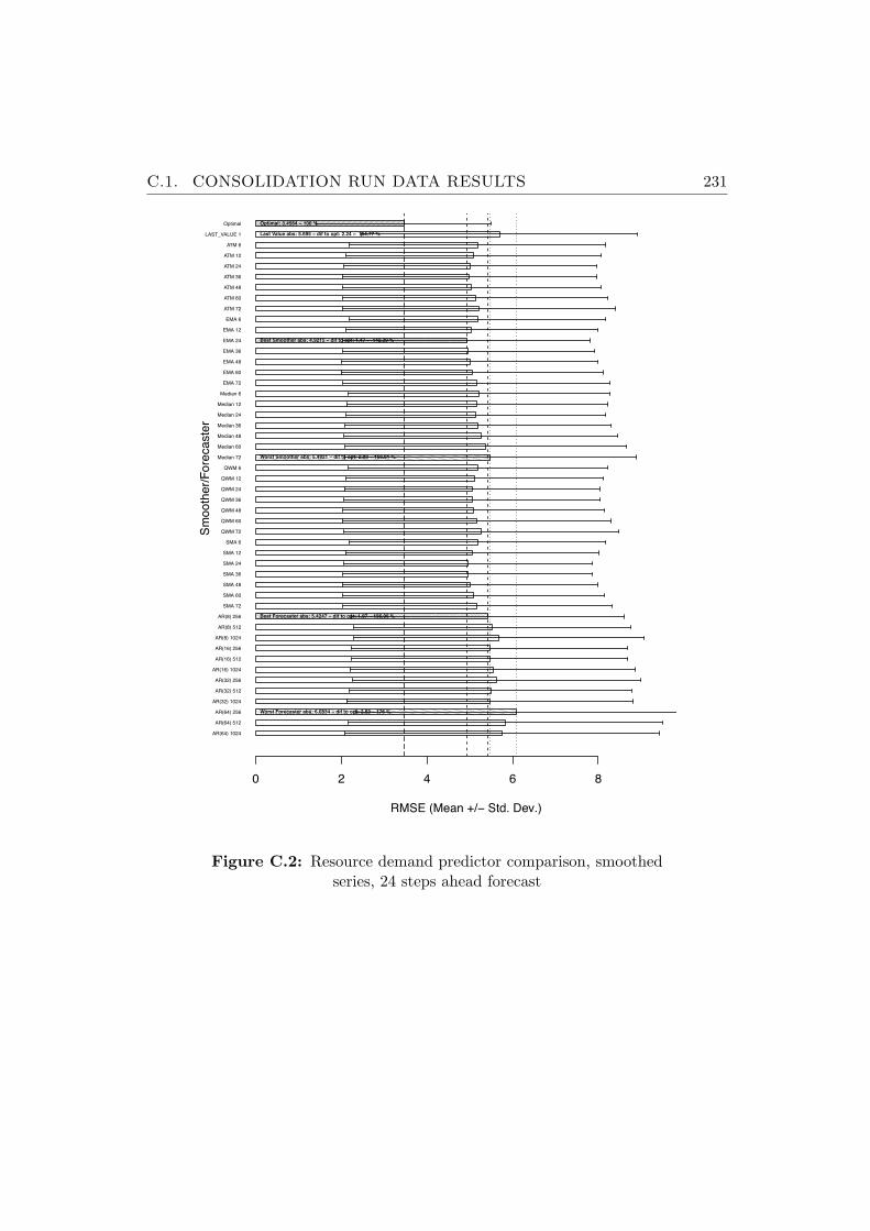
C.1. CONSOLIDATION RUN DATA RESULTS 231
AR(64) 1024
AR(64) 512
AR(64) 256
AR(32) 1024
AR(32) 512
AR(32) 256
AR(16) 1024
AR(16) 512
AR(16) 256
AR(8) 1024
AR(8) 512
AR(8) 256
SMA 72
SMA 60
SMA 48
SMA 36
SMA 24
SMA 12
SMA 6
QWM 72
QWM 60
QWM 48
QWM 36
QWM 24
QWM 12
QWM 6
Median 72
Median 60
Median 48
Median 36
Median 24
Median 12
Median 6
EMA 72
EMA 60
EMA 48
EMA 36
EMA 24
EMA 12
EMA 6
ATM 72
ATM 60
ATM 48
ATM 36
ATM 24
ATM 12
ATM 6
LAST_VALUE 1
Optimal
Optimal Forecaster vs. Smoother/Forecaster for Lookahead 24
RMSE (Mean +/! Std. Dev.)
Sm
ooth
er/
Fore
caste
r
0 2 4 6 8
Optimal: 3.4564 ! 100 %
Last Value abs: 5.695 ! dif to opt: 2.24 ! 164.77 %
Best Smoother abs: 4.9215 ! dif to opt: 1.47 ! 142.39 %
Worst Smoother abs: 5.4821 ! dif to opt: 2.03 ! 158.61 %
Best Forecaster abs: 5.4247 ! dif to opt: 1.97 ! 156.95 %
Worst Forecaster abs: 6.0834 ! dif to opt: 2.63 ! 176 %
Figure C.2: Resource demand predictor comparison, smoothedseries, 24 steps ahead forecast
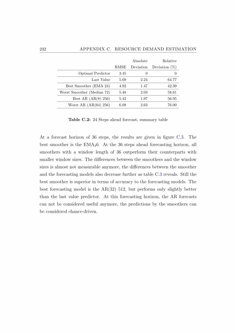
232 APPENDIX C. RESOURCE DEMAND ESTIMATION
Absolute Relative
RMSE Deviation Deviation (%)
Optimal Predictor 3.45 0 0
Last Value 5.69 2.24 64.77
Best Smoother (EMA 24) 4.92 1.47 42.39
Worst Smoother (Median 72) 5.48 2.03 58.61
Best AR (AR(8) 256) 5.42 1.97 56.95
Worst AR (AR(64) 256) 6.08 2.63 76.00
Table C.2: 24 Steps ahead forecast, summary table
At a forecast horizon of 36 steps, the results are given in figure C.3. The
best smoother is the EMA36. At the 36 steps ahead forecasting horizon, all
smoothers with a window length of 36 outperform their counterparts with
smaller window sizes. The differences between the smoothers and the window
sizes is almost not measurable anymore, the differences between the smoother
and the forecasting models also decrease further as table C.3 reveals. Still the
best smoother is superior in terms of accuracy to the forecasting models. The
best forecasting model is the AR(32) 512, but performs only slightly better
than the last value predictor. At this forecasting horizon, the AR forecasts
can not be considered useful anymore, the predictions by the smoothers can
be considered chance-driven.
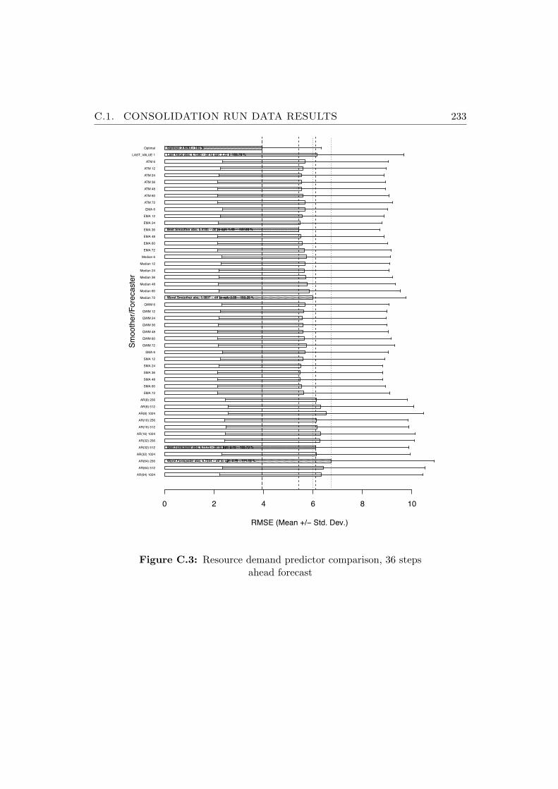
C.1. CONSOLIDATION RUN DATA RESULTS 233
AR(64) 1024
AR(64) 512
AR(64) 256
AR(32) 1024
AR(32) 512
AR(32) 256
AR(16) 1024
AR(16) 512
AR(16) 256
AR(8) 1024
AR(8) 512
AR(8) 256
SMA 72
SMA 60
SMA 48
SMA 36
SMA 24
SMA 12
SMA 6
QWM 72
QWM 60
QWM 48
QWM 36
QWM 24
QWM 12
QWM 6
Median 72
Median 60
Median 48
Median 36
Median 24
Median 12
Median 6
EMA 72
EMA 60
EMA 48
EMA 36
EMA 24
EMA 12
EMA 6
ATM 72
ATM 60
ATM 48
ATM 36
ATM 24
ATM 12
ATM 6
LAST_VALUE 1
Optimal
Optimal Forecaster vs. Smoother/Forecaster for Lookahead 36
RMSE (Mean +/! Std. Dev.)
Sm
ooth
er/
Fore
caste
r
0 2 4 6 8 10
Optimal: 3.9283 ! 100 %
Last Value abs: 6.1588 ! dif to opt: 2.23 ! 156.78 %
Best Smoother abs: 5.4185 ! dif to opt: 1.49 ! 137.93 %
Worst Smoother abs: 5.9807 ! dif to opt: 2.05 ! 152.25 %
Best Forecaster abs: 6.1175 ! dif to opt: 2.19 ! 155.73 %
Worst Forecaster abs: 6.7224 ! dif to opt: 2.79 ! 171.13 %
Figure C.3: Resource demand predictor comparison, 36 stepsahead forecast
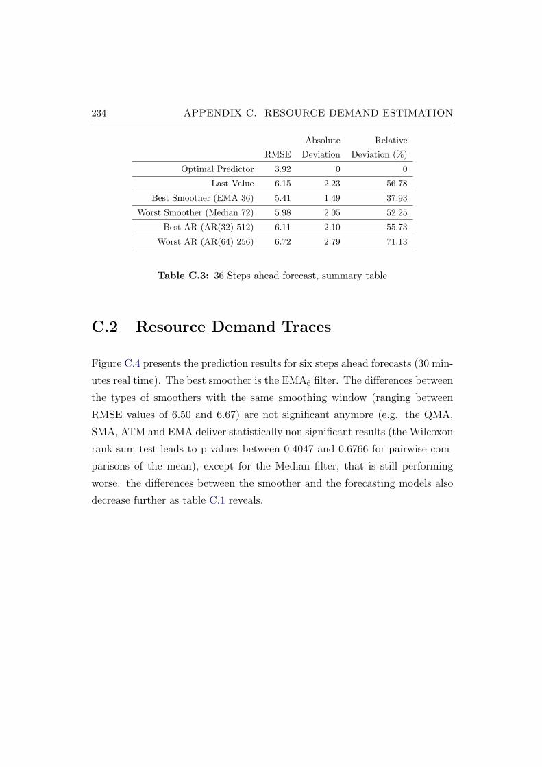
234 APPENDIX C. RESOURCE DEMAND ESTIMATION
Absolute Relative
RMSE Deviation Deviation (%)
Optimal Predictor 3.92 0 0
Last Value 6.15 2.23 56.78
Best Smoother (EMA 36) 5.41 1.49 37.93
Worst Smoother (Median 72) 5.98 2.05 52.25
Best AR (AR(32) 512) 6.11 2.10 55.73
Worst AR (AR(64) 256) 6.72 2.79 71.13
Table C.3: 36 Steps ahead forecast, summary table
C.2 Resource Demand Traces
Figure C.4 presents the prediction results for six steps ahead forecasts (30 min-
utes real time). The best smoother is the EMA6 filter. The differences between
the types of smoothers with the same smoothing window (ranging between
RMSE values of 6.50 and 6.67) are not significant anymore (e.g. the QMA,
SMA, ATM and EMA deliver statistically non significant results (the Wilcoxon
rank sum test leads to p-values between 0.4047 and 0.6766 for pairwise com-
parisons of the mean), except for the Median filter, that is still performing
worse. the differences between the smoother and the forecasting models also
decrease further as table C.1 reveals.
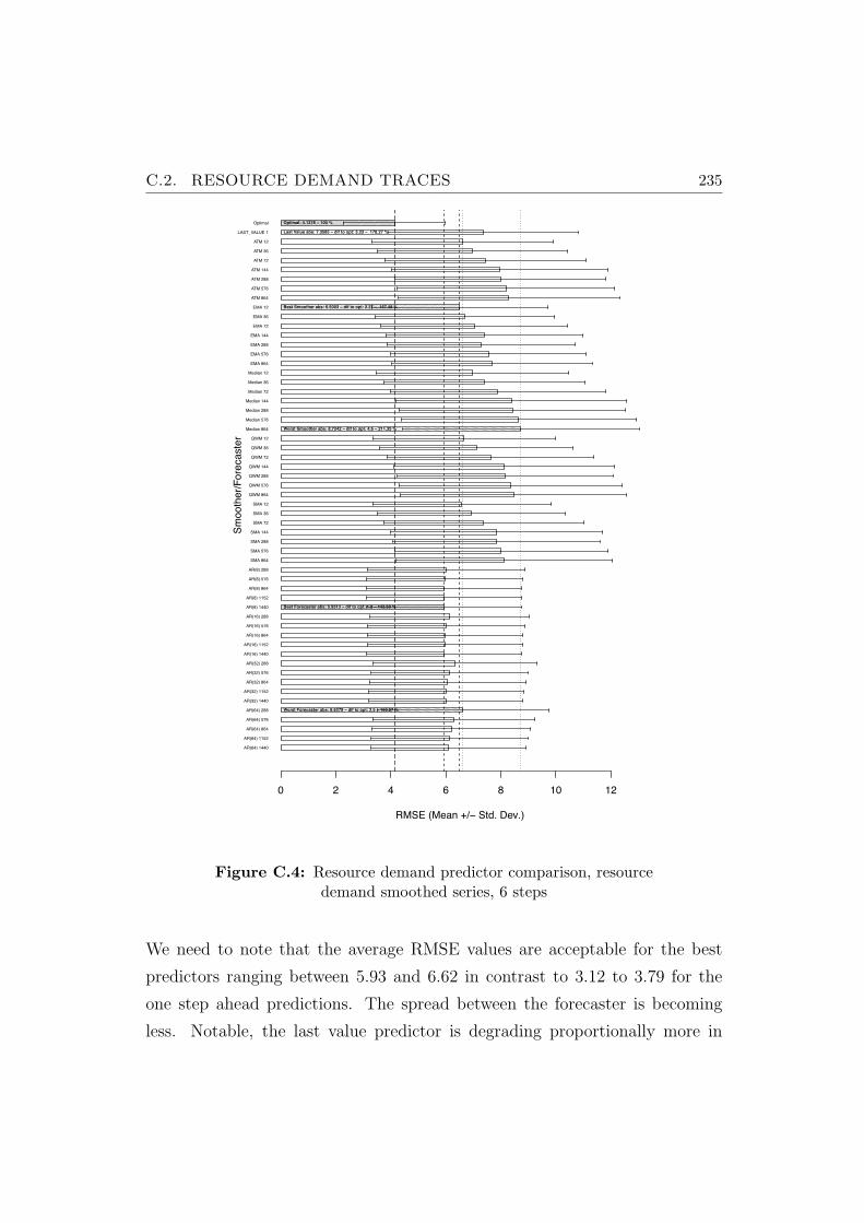
C.2. RESOURCE DEMAND TRACES 235
AR(64) 1440
AR(64) 1152
AR(64) 864
AR(64) 576
AR(64) 288
AR(32) 1440
AR(32) 1152
AR(32) 864
AR(32) 576
AR(32) 288
AR(16) 1440
AR(16) 1152
AR(16) 864
AR(16) 576
AR(16) 288
AR(8) 1440
AR(8) 1152
AR(8) 864
AR(8) 576
AR(8) 288
SMA 864
SMA 576
SMA 288
SMA 144
SMA 72
SMA 36
SMA 12
QWM 864
QWM 576
QWM 288
QWM 144
QWM 72
QWM 36
QWM 12
Median 864
Median 576
Median 288
Median 144
Median 72
Median 36
Median 12
EMA 864
EMA 576
EMA 288
EMA 144
EMA 72
EMA 36
EMA 12
ATM 864
ATM 576
ATM 288
ATM 144
ATM 72
ATM 36
ATM 12
LAST_VALUE 1
Optimal
Optimal Forecaster vs. Smoother/Forecaster for Lookahead 6
RMSE (Mean +/! Std. Dev.)
Sm
oo
the
r/F
ore
ca
ste
r
0 2 4 6 8 10 12
Optimal: 4.1278 ! 100 %
Last Value abs: 7.3585 ! dif to opt: 3.23 ! 178.27 %
Best Smoother abs: 6.5003 ! dif to opt: 2.37 ! 157.48 %
Worst Smoother abs: 8.7242 ! dif to opt: 4.6 ! 211.35 %
Best Forecaster abs: 5.9313 ! dif to opt: 1.8 ! 143.69 %
Worst Forecaster abs: 6.6279 ! dif to opt: 2.5 ! 160.57 %
Figure C.4: Resource demand predictor comparison, resourcedemand smoothed series, 6 steps
We need to note that the average RMSE values are acceptable for the best
predictors ranging between 5.93 and 6.62 in contrast to 3.12 to 3.79 for the
one step ahead predictions. The spread between the forecaster is becoming
less. Notable, the last value predictor is degrading proportionally more in
236 APPENDIX C. RESOURCE DEMAND ESTIMATION
accuracy then all other predictors.
Absolute Relative
RMSE Deviation Deviation (%)
Optimal Predictor 4.12 0 0
Last Value 7.35 3.23 78.27
Best Smoother (EMA 12) 6.50 2.38 57.40
Worst Smoother (Median 864) 8.72 4.60 111.35
Best AR (AR(8) 1440) 5.93 1.81 43.69
Worst AR (AR(64) 288) 6.62 2.50 60.57
Table C.4: Resource demand traces: 6 steps ahead forecast,summary table
Figure C.5 presents the prediction results for 24 steps, or two hours of real
time ahead forecasts. The best smoother is the EMA288. At the 24 steps
ahead forecasting horizon, all smoothers with a window length of 288 outper-
form their counterparts with smaller window sizes. This effect is due to the
daily demand patterns. The last value predictor is the worst predictor of all,
even outperformed by the worst smoother so far (Median864). The differences
between the best and the worst smoothers is further decreasing, the differences
between forecasting models also decrease further as table C.2 reveals. The best
forecasting is superior in terms of accuracy to the bets smoother. However the
large RMSE values indicate that the forecasts are not reliable anymore.

C.2. RESOURCE DEMAND TRACES 237
AR(64) 1440
AR(64) 1152
AR(64) 864
AR(64) 576
AR(64) 288
AR(32) 1440
AR(32) 1152
AR(32) 864
AR(32) 576
AR(32) 288
AR(16) 1440
AR(16) 1152
AR(16) 864
AR(16) 576
AR(16) 288
AR(8) 1440
AR(8) 1152
AR(8) 864
AR(8) 576
AR(8) 288
SMA 864
SMA 576
SMA 288
SMA 144
SMA 72
SMA 36
SMA 12
QWM 864
QWM 576
QWM 288
QWM 144
QWM 72
QWM 36
QWM 12
Median 864
Median 576
Median 288
Median 144
Median 72
Median 36
Median 12
EMA 864
EMA 576
EMA 288
EMA 144
EMA 72
EMA 36
EMA 12
ATM 864
ATM 576
ATM 288
ATM 144
ATM 72
ATM 36
ATM 12
LAST_VALUE 1
Optimal
Optimal Forecaster vs. Smoother/Forecaster for Lookahead 24
RMSE (Mean +/! Std. Dev.)
Sm
oo
the
r/F
ore
ca
ste
r
0 2 4 6 8 10 12 14
Optimal: 5.1166 ! 100 %
Last Value abs: 9.6381 ! dif to opt: 4.52 ! 188.37 %
Best Smoother abs: 7.7051 ! dif to opt: 2.59 ! 150.59 %
Worst Smoother abs: 8.7779 ! dif to opt: 3.66 ! 171.56 %
Best Forecaster abs: 7.3752 ! dif to opt: 2.26 ! 144.14 %
Worst Forecaster abs: 7.9973 ! dif to opt: 2.88 ! 156.3 %
Figure C.5: Resource demand predictor comparison, resourcedemand smoothed series, 24 steps
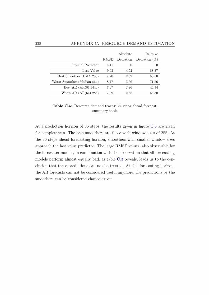
238 APPENDIX C. RESOURCE DEMAND ESTIMATION
Absolute Relative
RMSE Deviation Deviation (%)
Optimal Predictor 5.11 0 0
Last Value 9.63 4.52 88.37
Best Smoother (EMA 288) 7.70 2.59 50.50
Worst Smoother (Median 864) 8.77 3.66 71.56
Best AR (AR(8) 1440) 7.37 2.26 44.14
Worst AR (AR(64) 288) 7.99 2.88 56.30
Table C.5: Resource demand traces: 24 steps ahead forecast,summary table
At a prediction horizon of 36 steps, the results given in figure C.6 are given
for completeness. The best smoothers are those with window sizes of 288. At
the 36 steps ahead forecasting horizon, smoothers with smaller window sizes
approach the last value predictor. The large RMSE values, also observable for
the forecaster models, in combination with the observation that all forecasting
models perform almost equally bad, as table C.3 reveals, leads us to the con-
clusion that these predictions can not be trusted. At this forecasting horizon,
the AR forecasts can not be considered useful anymore, the predictions by the
smoothers can be considered chance driven.
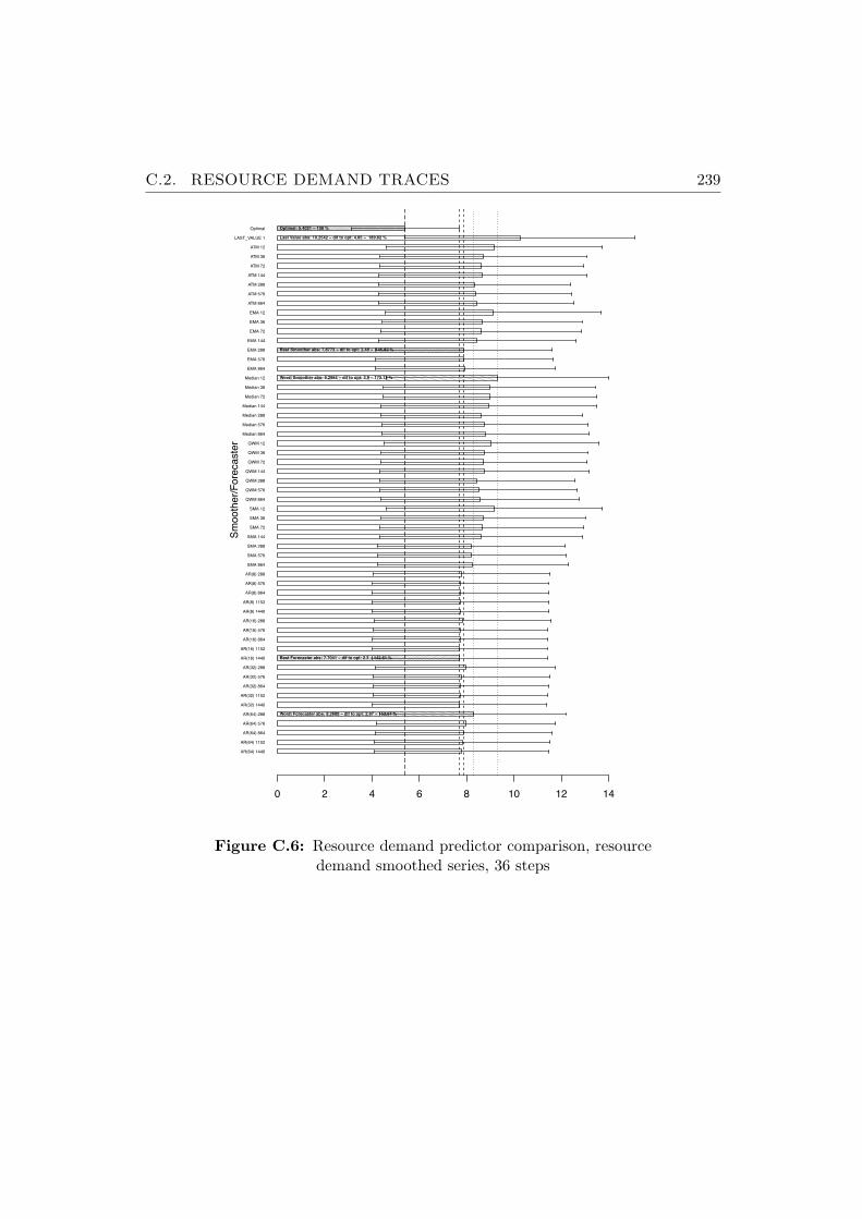
C.2. RESOURCE DEMAND TRACES 239
AR(64) 1440
AR(64) 1152
AR(64) 864
AR(64) 576
AR(64) 288
AR(32) 1440
AR(32) 1152
AR(32) 864
AR(32) 576
AR(32) 288
AR(16) 1440
AR(16) 1152
AR(16) 864
AR(16) 576
AR(16) 288
AR(8) 1440
AR(8) 1152
AR(8) 864
AR(8) 576
AR(8) 288
SMA 864
SMA 576
SMA 288
SMA 144
SMA 72
SMA 36
SMA 12
QWM 864
QWM 576
QWM 288
QWM 144
QWM 72
QWM 36
QWM 12
Median 864
Median 576
Median 288
Median 144
Median 72
Median 36
Median 12
EMA 864
EMA 576
EMA 288
EMA 144
EMA 72
EMA 36
EMA 12
ATM 864
ATM 576
ATM 288
ATM 144
ATM 72
ATM 36
ATM 12
LAST_VALUE 1
Optimal
Optimal Forecaster vs. Smoother/Forecaster for Lookahead 36
RMSE (Mean +/! Std. Dev.)
Sm
oo
the
r/F
ore
ca
ste
r
0 2 4 6 8 10 12 14
Optimal: 5.4021 ! 100 %
Last Value abs: 10.2542 ! dif to opt: 4.85 ! 189.82 %
Best Smoother abs: 7.8773 ! dif to opt: 2.48 ! 145.82 %
Worst Smoother abs: 9.2984 ! dif to opt: 3.9 ! 172.13 %
Best Forecaster abs: 7.7041 ! dif to opt: 2.3 ! 142.61 %
Worst Forecaster abs: 8.2688 ! dif to opt: 2.87 ! 153.07 %
Figure C.6: Resource demand predictor comparison, resourcedemand smoothed series, 36 steps
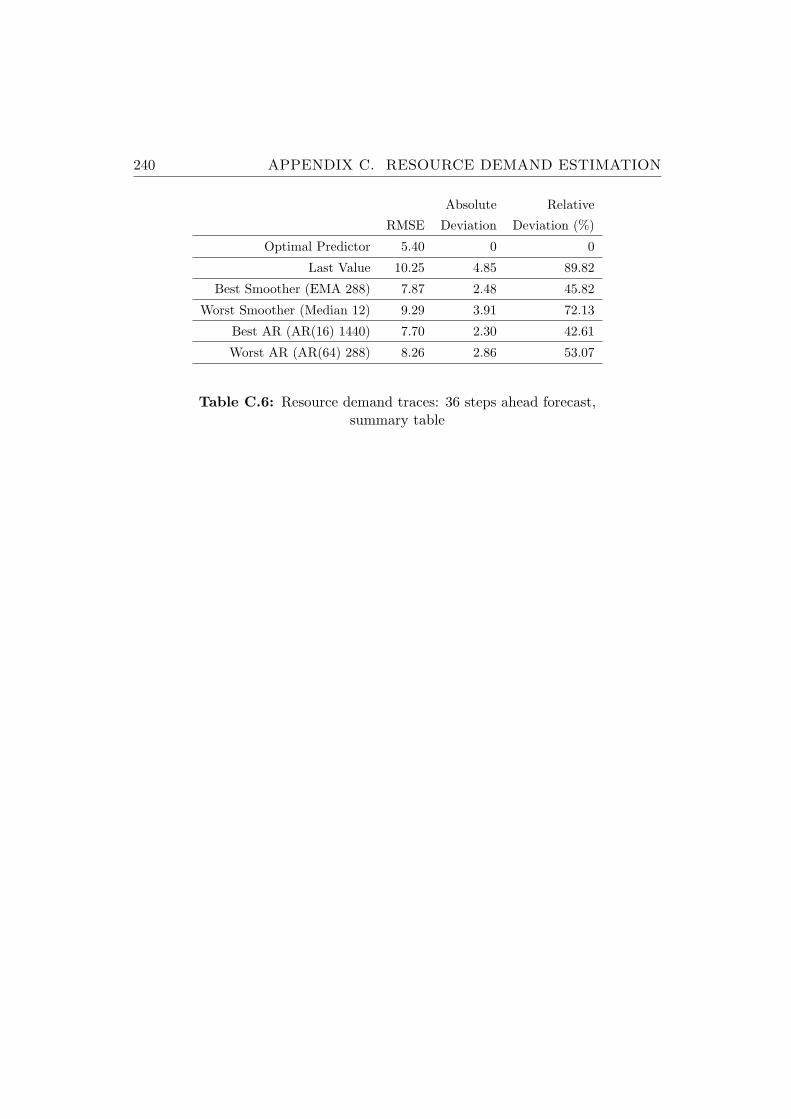
240 APPENDIX C. RESOURCE DEMAND ESTIMATION
Absolute Relative
RMSE Deviation Deviation (%)
Optimal Predictor 5.40 0 0
Last Value 10.25 4.85 89.82
Best Smoother (EMA 288) 7.87 2.48 45.82
Worst Smoother (Median 12) 9.29 3.91 72.13
Best AR (AR(16) 1440) 7.70 2.30 42.61
Worst AR (AR(64) 288) 8.26 2.86 53.07
Table C.6: Resource demand traces: 36 steps ahead forecast,summary table
Appendix D
Reactive Control versus
Overbooking
In the following sections we will give a comparison on the response times and
efficiency achieved by overbooking resources in contrast to:
The expected case: Finding the right control parameters for a reactive control
system is dependent on the overall workload characteristics and other factors.
However, if we assume a clairvoyant control strategy that requires a minimum
of migrations the impact on the quality of service metrics of an application may
be much lower than what we achieved in our runs. Hence, in the expected case
we compare the efficiency of overbooking against the baseline consolidation
efficiency and response times. We assume no increase in response times that
would be incurred by control actions.
The minimum case: We select the reactive run from all runs executed in the
experiment groups 1 - 11 that delivered the best average response time and
compare, on a scenario basis, the delivered efficiency and response times with
the same metrics achieved by overbooking by a given percentage.
The maximum case: We select the reactive run from all runs executed in the
241
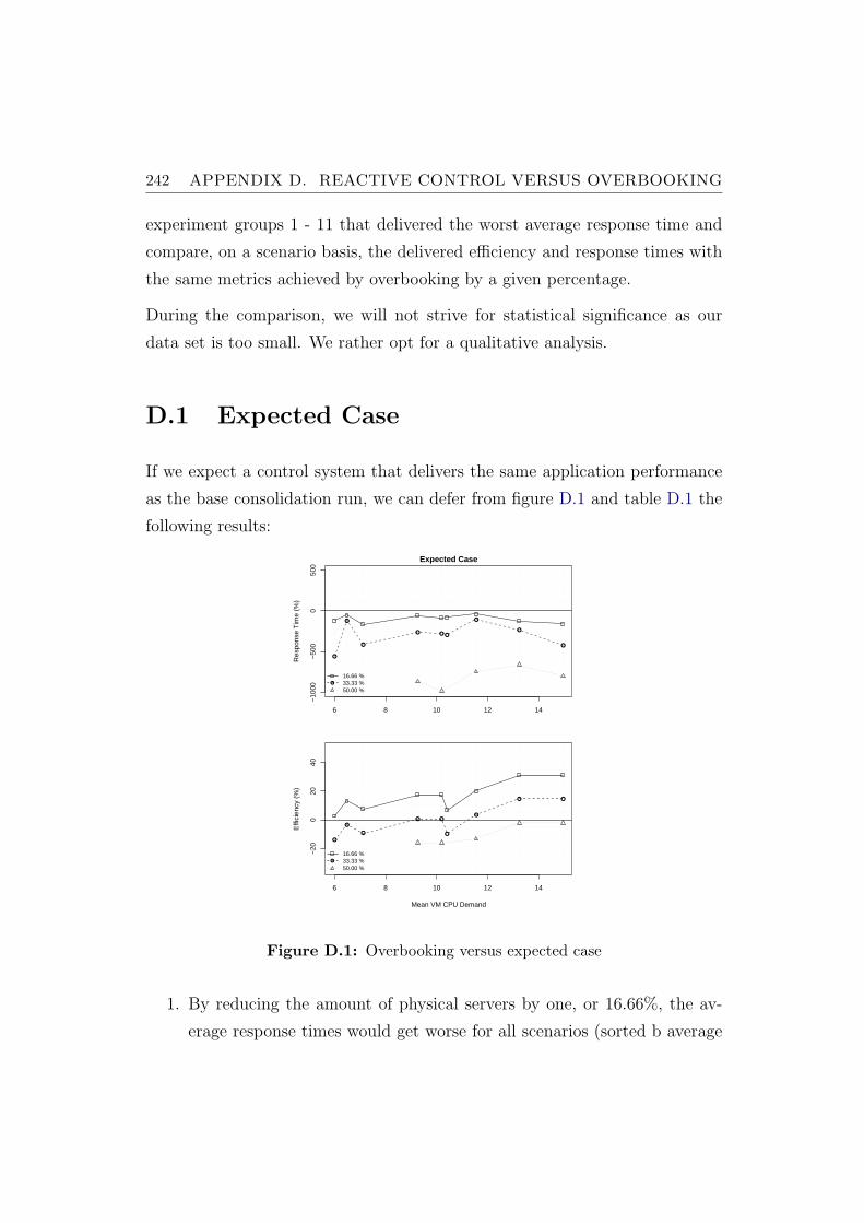
242 APPENDIX D. REACTIVE CONTROL VERSUS OVERBOOKING
experiment groups 1 - 11 that delivered the worst average response time and
compare, on a scenario basis, the delivered efficiency and response times with
the same metrics achieved by overbooking by a given percentage.
During the comparison, we will not strive for statistical significance as our
data set is too small. We rather opt for a qualitative analysis.
D.1 Expected Case
If we expect a control system that delivers the same application performance
as the base consolidation run, we can defer from figure D.1 and table D.1 the
following results:
6 8 10 12 14
−10
00−
500
050
0
Expected Case
Res
pons
e T
ime
(%)
●
●
●
● ● ●
●
●
●
●
16.66 %33.33 %50.00 %
6 8 10 12 14
−20
020
40
Mean VM CPU Demand
Effi
cien
cy (
%)
●
●
●
● ●
●
●
● ●
●
16.66 %33.33 %50.00 %
Figure D.1: Overbooking versus expected case
1. By reducing the amount of physical servers by one, or 16.66%, the av-
erage response times would get worse for all scenarios (sorted b average
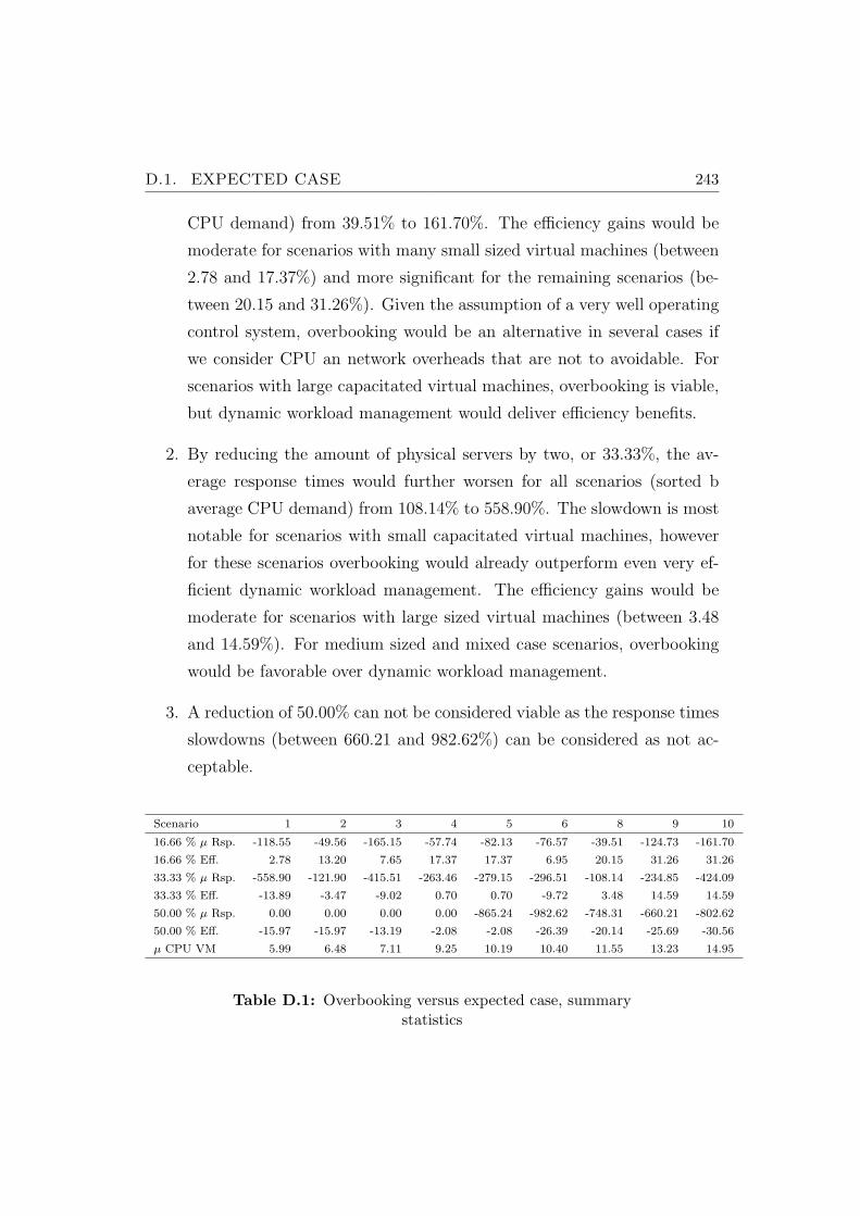
D.1. EXPECTED CASE 243
CPU demand) from 39.51% to 161.70%. The efficiency gains would be
moderate for scenarios with many small sized virtual machines (between
2.78 and 17.37%) and more significant for the remaining scenarios (be-
tween 20.15 and 31.26%). Given the assumption of a very well operating
control system, overbooking would be an alternative in several cases if
we consider CPU an network overheads that are not to avoidable. For
scenarios with large capacitated virtual machines, overbooking is viable,
but dynamic workload management would deliver efficiency benefits.
2. By reducing the amount of physical servers by two, or 33.33%, the av-
erage response times would further worsen for all scenarios (sorted b
average CPU demand) from 108.14% to 558.90%. The slowdown is most
notable for scenarios with small capacitated virtual machines, however
for these scenarios overbooking would already outperform even very ef-
ficient dynamic workload management. The efficiency gains would be
moderate for scenarios with large sized virtual machines (between 3.48
and 14.59%). For medium sized and mixed case scenarios, overbooking
would be favorable over dynamic workload management.
3. A reduction of 50.00% can not be considered viable as the response times
slowdowns (between 660.21 and 982.62%) can be considered as not ac-
ceptable.
Scenario 1 2 3 4 5 6 8 9 10
16.66 % µ Rsp. -118.55 -49.56 -165.15 -57.74 -82.13 -76.57 -39.51 -124.73 -161.70
16.66 % Eff. 2.78 13.20 7.65 17.37 17.37 6.95 20.15 31.26 31.26
33.33 % µ Rsp. -558.90 -121.90 -415.51 -263.46 -279.15 -296.51 -108.14 -234.85 -424.09
33.33 % Eff. -13.89 -3.47 -9.02 0.70 0.70 -9.72 3.48 14.59 14.59
50.00 % µ Rsp. 0.00 0.00 0.00 0.00 -865.24 -982.62 -748.31 -660.21 -802.62
50.00 % Eff. -15.97 -15.97 -13.19 -2.08 -2.08 -26.39 -20.14 -25.69 -30.56
µ CPU VM 5.99 6.48 7.11 9.25 10.19 10.40 11.55 13.23 14.95
Table D.1: Overbooking versus expected case, summarystatistics
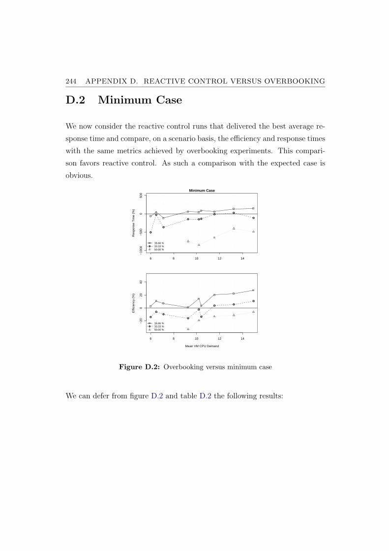
244 APPENDIX D. REACTIVE CONTROL VERSUS OVERBOOKING
D.2 Minimum Case
We now consider the reactive control runs that delivered the best average re-
sponse time and compare, on a scenario basis, the efficiency and response times
with the same metrics achieved by overbooking experiments. This compari-
son favors reactive control. As such a comparison with the expected case is
obvious.
6 8 10 12 14
−10
00−
500
050
0
Minimum Case
Res
pons
e T
ime
(%)
●
●
●
● ● ●
●●
●
●
16.66 %33.33 %50.00 %
6 8 10 12 14
−20
020
40
Mean VM CPU Demand
Effi
cien
cy (
%)
●
●
●
●
●
●
●●
●
●
16.66 %33.33 %50.00 %
Figure D.2: Overbooking versus minimum case
We can defer from figure D.2 and table D.2 the following results:
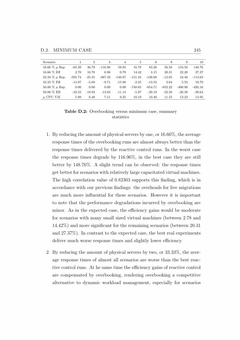
D.2. MINIMUM CASE 245
Scenario 1 2 3 4 5 6 8 9 10
16.66 % µ Rsp. -65.39 46.79 -116.96 58.85 45.78 83.26 56.58 134.58 148.76
16.66 % Eff. 2.70 10.78 6.96 0.79 14.42 3.15 20.31 22.20 27.37
33.33 % µ Rsp. -505.74 -25.55 -367.32 -146.87 -151.24 -136.68 -12.05 24.46 -113.63
33.33 % Eff. -13.97 -5.89 -9.71 -15.88 -2.25 -13.52 3.64 5.53 10.70
50.00 % µ Rsp. 0.00 0.00 0.00 0.00 -748.65 -854.71 -652.22 -400.90 -492.16
50.00 % Eff. -32.55 -18.92 -13.03 -11.14 -5.97 -30.19 -22.56 -26.38 -30.64
µ CPU VM 5.99 6.48 7.11 9.25 10.19 10.40 11.55 13.23 14.95
Table D.2: Overbooking versus minimum case, summarystatistics
1. By reducing the amount of physical servers by one, or 16.66%, the average
response times of the overbooking runs are almost always better than the
response times delivered by the reactive control runs. In the worst case
the response times degrade by 116.96%, in the best case they are still
better by 148.76%. A slight trend can be observed: the response times
get better for scenarios with relatively large capacitated virtual machines.
The high correlation value of 0.82303 supports this finding, which is in
accordance with our previous findings: the overheads for live migrations
are much more influential for these scenarios. However it is important
to note that the performance degradations incurred by overbooking are
minor. As in the expected case, the efficiency gains would be moderate
for scenarios with many small sized virtual machines (between 2.78 and
14.42%) and more significant for the remaining scenarios (between 20.31
and 27.37%). In contrast to the expected case, the best real experiments
deliver much worse response times and slightly lower efficiency.
2. By reducing the amount of physical servers by two, or 33.33%, the aver-
age response times of almost all scenarios are worse than the best reac-
tive control runs. At he same time the efficiency gains of reactive control
are compensated by overbooking, rendering overbooking a competitive
alternative to dynamic workload management, especially for scenarios
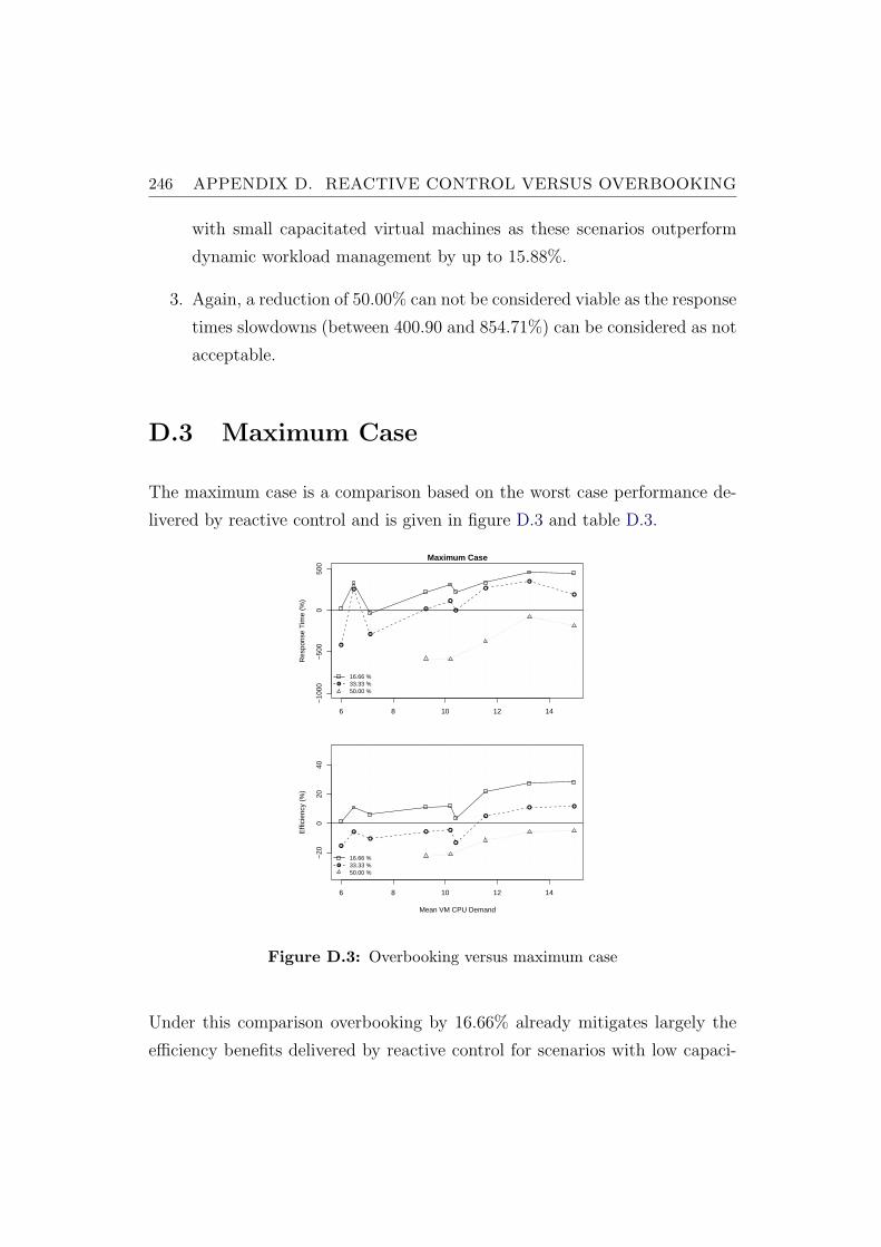
246 APPENDIX D. REACTIVE CONTROL VERSUS OVERBOOKING
with small capacitated virtual machines as these scenarios outperform
dynamic workload management by up to 15.88%.
3. Again, a reduction of 50.00% can not be considered viable as the response
times slowdowns (between 400.90 and 854.71%) can be considered as not
acceptable.
D.3 Maximum Case
The maximum case is a comparison based on the worst case performance de-
livered by reactive control and is given in figure D.3 and table D.3.
6 8 10 12 14
−10
00−
500
050
0
Maximum Case
Res
pons
e T
ime
(%)
●
●
●
●
●
●
●
●
●
●
16.66 %33.33 %50.00 %
6 8 10 12 14
−20
020
40
Mean VM CPU Demand
Effi
cien
cy (
%)
●
●
●
● ●
●
●
● ●
●
16.66 %33.33 %50.00 %
Figure D.3: Overbooking versus maximum case
Under this comparison overbooking by 16.66% already mitigates largely the
efficiency benefits delivered by reactive control for scenarios with low capaci-
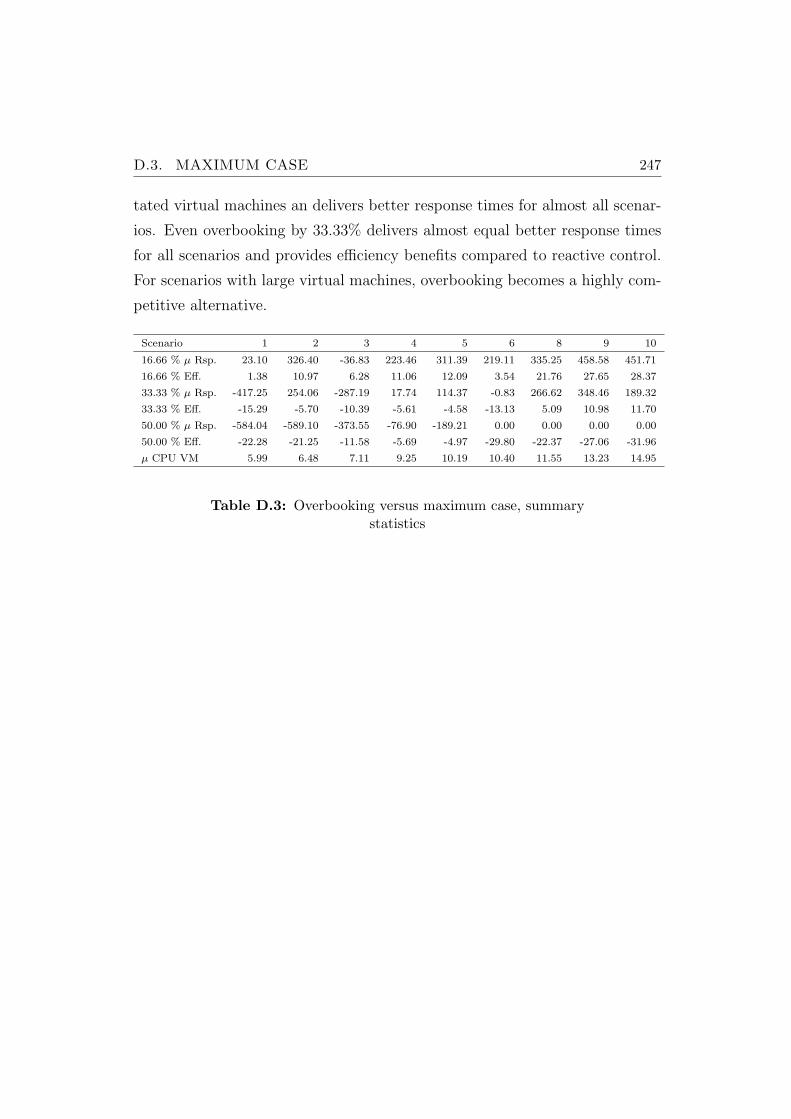
D.3. MAXIMUM CASE 247
tated virtual machines an delivers better response times for almost all scenar-
ios. Even overbooking by 33.33% delivers almost equal better response times
for all scenarios and provides efficiency benefits compared to reactive control.
For scenarios with large virtual machines, overbooking becomes a highly com-
petitive alternative.
Scenario 1 2 3 4 5 6 8 9 10
16.66 % µ Rsp. 23.10 326.40 -36.83 223.46 311.39 219.11 335.25 458.58 451.71
16.66 % Eff. 1.38 10.97 6.28 11.06 12.09 3.54 21.76 27.65 28.37
33.33 % µ Rsp. -417.25 254.06 -287.19 17.74 114.37 -0.83 266.62 348.46 189.32
33.33 % Eff. -15.29 -5.70 -10.39 -5.61 -4.58 -13.13 5.09 10.98 11.70
50.00 % µ Rsp. -584.04 -589.10 -373.55 -76.90 -189.21 0.00 0.00 0.00 0.00
50.00 % Eff. -22.28 -21.25 -11.58 -5.69 -4.97 -29.80 -22.37 -27.06 -31.96
µ CPU VM 5.99 6.48 7.11 9.25 10.19 10.40 11.55 13.23 14.95
Table D.3: Overbooking versus maximum case, summarystatistics
Bibliography
Abdelzaher, Tarek F., Kang G. Shin, Nina Bhatti. 2002. Performance guar-
antees for web server end-systems: A control-theoretical approach. IEEE
Transactions on Parallel and Distributed Systems 13 2002.
Ali, Shoukat, Jong-Kook Kim, Howard Jay Siegel, Anthony A. Maciejewski.
2008. Static heuristics for robust resource allocation of continuously execut-
ing applications. Journal on Parallel Distributed Computing 68 1070–1080.
Andreolini, Mauro, Sara Casolari, Michele Colajanni. 2008. Models and frame-
work for supporting runtime decisions in web-based systems. ACM Trans-
actions on the Web 2(3) 1 – 43.
Andrzejak, Artur, Sven Graupner, Stefan Plantikow. 2006. Predicting resource
demand in dynamic utility computing environments. Proceedings of the
International Conference on Autonomic and Autonomous Systems . ICAS
’06, IEEE Computer Society, Washington, DC, USA, 6–18. doi:10.1109/
ICAS.2006.44.
Appleby, K., S. Fakhouri, L. Fong, G. Goldszmidt, M. Kalantar, S. Krish-
nakumar, D.P. Pazel, J. Pershing, B. Rochwerger. 2001. Oceano-SLA based
management of a computing utility. IEEE/IFIP International Symposium
on Integrated Network Management . 855 – 868.
Arlitt, Martin F., Carey L. Williamson. 1997. Internet web servers: work-
248
BIBLIOGRAPHY 249
load characterization and performance implications. IEEE Transaction on
Networks 5(5) 631–645.
Bansal, Nikhil, Alberto Caprara, Maxim Sviridenko. 2009. A new approxima-
tion method for set covering problems, with applications to multidimensional
bin packing. SIAM Journal on Computing 39(4) 1256–1278.
Barham, Paul, Boris Dragovic, Keir Fraser, Steven Hand, Tim Harris, Alex
Ho, Rolf Neugebauer, Ian Pratt, Andrew Warfield. 2003. Xen and the art
of virtualization. SOSP ’03: Proceedings of the nineteenth ACM symposium
on Operating systems principles . ACM, New York, NY, USA, 164–177.
Baryshnikov, Yuliy, Ed Coffman, Guillaume Pierre, Dan Rubenstein, Mark
Squillante, Teddy Yimwadsana. 2005. Predictability of web-server traffic
congestion. Proceedings of the 10th International Workshop on Web Content
Caching and Distribution. IEEE Computer Society, Washington, DC, USA,
97–103.
Blagodurov, Sergey, Sergey Zhuravlev, Alexandra Fedorova. 2010. Contention-
aware scheduling on multicore systems. ACM Transactions on Computer
Systems 28(4) 1– 45.
Bobroff, Norman, Andrzej Kochut, Kirk Beaty. 2007. Dynamic placement of
virtual machines for managing sla violations. Integrated Network Manage-
ment . IEEE, 119–128.
Bodik, Peter, Rean Griffith, Charles Sutton, Armando Fox, Michael I. Jordan,
David A. Patterson. 2009. Automatic exploration of datacenter performance
regimes. Proceedings of the 1st workshop on Automated control for datacen-
ters and clouds . ACDC ’09, New York, NY, USA, 1–6.
Bowerman, Bruce L., Richard O’Connell, Anne Koehler. 2004. Forecasting,
Time Series, and Regression: An Applied Approach. South-Western College
Pub.
250 BIBLIOGRAPHY
Box, George E. P., Gwilym M. Jenkins, Gregory C. Reinsel. 2008. Time Series
Analysis: Forecasting and Control . John Wiley & Sons.
Bradford, Robert, Evangelos Kotsovinos, Anja Feldmann, Harald Schioberg.
2007. Live wide-area migration of virtual machines including local persistent
state. Proceedings of the 3rd international conference on Virtual execution
environments . VEE ’07, ACM, New York, NY, USA, 169–179.
Breitgand, D., M. Goldstein, E.H. Shehory. 2011. Efficient control of false
negative and false positive errors with separate adaptive thresholds. IEEE
Transactions on Network and Service Management 8(2) 128 –140.
Brown, Richard, Alliance to Save Energy, ICF Incorporated, ERG Incorpo-
rated, U.S. Environmental Protection Agency. 2008. Report to congress on
server and data center energy efficiency: Public law 109-431.
Bulpin, James R., Ian A. Pratt. 2004. Multiprogramming performance of the
pentium 4 with hyper-threading. Third Annual Workshop on Duplicating,
Deconstruction and Debunking (at ISCA’04). 53–62.
Bulpin, James R., Ian A. Pratt. 2005. Hyper-threading aware process schedul-
ing heuristics. Proceedings of the annual conference on USENIX Annual
Technical Conference. ATEC ’05, USENIX Association, Berkeley, CA, USA,
27–32.
Burgess, Mark, Harek Haugerud, Sigmund Straumsnes, Trond Reitan. 2002.
Measuring system normality. ACM Transactions on Computer Systems
20(2) 125–160.
Casale, Giuliano, Amir Kalbasi, Diwakar Krishnamurthy, Jerry Rolia. 2009.
Automatically generating bursty benchmarks for multitier systems. SIG-
METRICS Performance Evaluation Review 37(3) 32–37.
BIBLIOGRAPHY 251
Casolari, Sara, Michele Colajanni. 2009. Short-term prediction models for
server management in internet-based contexts. Decision Support Systems
48 212–223.
Chan, Joseph Wun-Tat, Tak-Wah Lam, Prudence W. H. Wong. 2008. Dynamic
bin packing of unit fractions items. Theoretical Computer Science 409 521–
529.
Chandra, Dhruba, Fei Guo, Seongbeom Kim, Yan Solihin. 2005. Predicting
inter-thread cache contention on a chip multi-processor architecture. Pro-
ceedings of the 11th International Symposium on High-Performance Com-
puter Architecture. IEEE Computer Society, Washington, DC, USA, 340–
351.
Chase, Jeffrey S., Darrell C. Anderson, Prachi N. Thakar, Amin M. Vahdat,
Ronald P. Doyle. 2001. Managing energy and server resources in hosting cen-
ters. SOSP ’01: Proceedings of the eighteenth ACM symposium on Operating
systems principles . ACM, New York, NY, USA, 103–116.
Chekuri, Chandra, Sanjeev Khanna. 2004. On multidimensional packing prob-
lems. SIAM Journal of Computing 33 837–851.
Chen, Wenzhi, Huijun Chen, Wei Huang, Xiaoqin Chen, Dapeng Huang. 2010.
Improving host swapping using adaptive prefetching and paging notifier.
Proceedings of the 19th ACM International Symposium on High Performance
Distributed Computing . HPDC ’10, New York, NY, USA, 300–303.
Chen, X., J. Heidemann. 2005. Flash crowd mitigation via adaptive admis-
sion control based on application-level observation. ACM Transactions on
Internet Technology 5(3) 532–562.
Chen, Xuan, John Heidemann. 2002. Flash crowd mitigation via an adaptive
admission control based on application-level measurement. Tech. Rep. ISI-
TR-557, USC/Information Sciences Institute.
252 BIBLIOGRAPHY
Cherkasova, Ludmila, Diwaker Gupta, Amin Vahdat. 2007. Comparison of the
three cpu schedulers in xen. SIGMETRICS Performance Evaluation Review
35 42–51.
Cherkasova, Ludmila, Kivanc Ozonat, Ningfang Mi, Julie Symons, Evgenia
Smirni. 2009. Automated anomaly detection and performance modeling of
enterprise applications. ACM Transactions on Computer Systems 27 1– 32.
Cherkasova, Ludmila, Peter Phaal. 2002. Session-based admission control:
A mechanism for peak load management of commercial web sites. IEEE
Transactions on Computers 51 669 – 685.
Citrix. 2012. Citrix xenserver. URL http://www.citrix.de/produkte/
xenserver/.
Coffman, Edward G., Jr. Jnos, Csirik Lajos Rnyai, Ambrus Zsbn. 1983. Dy-
namic bin packing. SIAM Journal of Computing 12 227–258.
Csirik, Jnos, J. B. G. Frenk, Martine Labb, Shuzhong Zhang. 1990. On the
multidimensional vector bin packing. Acta Cyberntica 361–369.
Dahlin, Michael. 2000. Interpreting stale load information. IEEE Transactions
on Parallel Distributed Systems 11 1033–1047.
Dhiman, Gaurav, Giacomo Marchetti, Tajana Rosing. 2010. vGreen: A System
for Energy-Efficient Management of Virtual Machines. ACM Transactions
on Design Automation of Electronic Systems 16 6:1–6:27.
Diao, Yixin, Joseph L. Hellerstein, Sujay Parekh, Rean Griffith, Gail Kaiser,
Dan Phung. 2005. Self-managing systems: A control theory foundation.
Proceedings of the 12th IEEE International Conference on Engineering of
Computer-Based Systems . IEEE Computer Society, Washington, DC, USA,
441–448.

BIBLIOGRAPHY 253
Dinda, Peter A. 1999. The statistical properties of host load. Scientific Pro-
gramming 7 211–229.
Dinda, Peter A., David R. O’Hallaron. 2000. Host load prediction using linear
models. Cluster Computing 3(4) 265–280.
Dosa, Gyorgy. 2007. The tight bound of first fit decreasing bin-packing al-
gorithm is ffd(i)=(11/9)opt(i)+6/9. Bo Chen, Mike Paterson, Guochuan
Zhang, eds., Combinatorics, Algorithms, Probabilistic and Experimental
Methodologies , Lecture Notes in Computer Science, vol. 4614. Springer
Berlin / Heidelberg, 1–11.
Duffield, N.G., F. Lo Presti. 2002. Multicast inference of packet delay vari-
ance at interior network links. Proceedings of the 19th IEEE International
Conference on Compute Communications , vol. 3. 1351–1360.
E. Limpert, W.A. Stahel, M. Abbt. 2001. Lognormal distributions across the
sciences: keys and clues. Bioscience 51(5) 341–352.
Engle, Robert F. 1982. Autoregressive conditional heteroscedasticity with es-
timates of the variance of united kingdom inflation. Econometrica 50(4)
987–1007.
Faban. 2012. URL http://java.net/projects/faban/.
Fernandez de la Vega, W., G. Lueker. 1981. Bin packing can be solved within
1 + e in linear time. Combinatorica 1 349–355.
Gmach, D., S. Krompass, A. Scholz, M. Wimmer, A. Kemper. 2008. Adaptive
quality of service management for enterprise services. ACM Transactions
on the Web 2(1) 1– 46.
Gmach, Daniel, Jerry Rolia, Ludmila Cherkasova, Alfons Kemper. 2007. Work-
load analysis and demand prediction of enterprise data center applications.
IISWC ’07: Proceedings of the 2007 IEEE 10th International Symposium
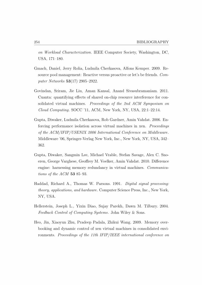
254 BIBLIOGRAPHY
on Workload Characterization. IEEE Computer Society, Washington, DC,
USA, 171–180.
Gmach, Daniel, Jerry Rolia, Ludmila Cherkasova, Alfons Kemper. 2009. Re-
source pool management: Reactive versus proactive or let’s be friends. Com-
puter Networks 53(17) 2905–2922.
Govindan, Sriram, Jie Liu, Aman Kansal, Anand Sivasubramaniam. 2011.
Cuanta: quantifying effects of shared on-chip resource interference for con-
solidated virtual machines. Proceedings of the 2nd ACM Symposium on
Cloud Computing . SOCC ’11, ACM, New York, NY, USA, 22:1–22:14.
Gupta, Diwaker, Ludmila Cherkasova, Rob Gardner, Amin Vahdat. 2006. En-
forcing performance isolation across virtual machines in xen. Proceedings
of the ACM/IFIP/USENIX 2006 International Conference on Middleware.
Middleware ’06, Springer-Verlag New York, Inc., New York, NY, USA, 342–
362.
Gupta, Diwaker, Sangmin Lee, Michael Vrable, Stefan Savage, Alex C. Sno-
eren, George Varghese, Geoffrey M. Voelker, Amin Vahdat. 2010. Difference
engine: harnessing memory redundancy in virtual machines. Communica-
tions of the ACM 53 85–93.
Haddad, Richard A., Thomas W. Parsons. 1991. Digital signal processing:
theory, applications, and hardware. Computer Science Press, Inc., New York,
NY, USA.
Hellerstein, Joseph L., Yixin Diao, Sujay Parekh, Dawn M. Tilbury. 2004.
Feedback Control of Computing Systems . John Wiley & Sons.
Heo, Jin, Xiaoyun Zhu, Pradeep Padala, Zhikui Wang. 2009. Memory over-
booking and dynamic control of xen virtual machines in consolidated envi-
ronments. Proceedings of the 11th IFIP/IEEE international conference on
BIBLIOGRAPHY 255
Symposium on Integrated Network Management . IM’09, IEEE Press, Piscat-
away, NJ, USA, 630–637.
Hermenier, Fabien, Xavier Lorca, Jean-Marc Menaud, Gilles Muller, Julia
Lawall. 2009. Entropy: a consolidation manager for clusters. Proceedings
of the 2009 ACM SIGPLAN/SIGOPS international conference on Virtual
execution environments . VEE ’09, New York, NY, USA, 41–50.
Hines, Michael R., Umesh Deshpande, Kartik Gopalan. 2009. Post-copy live
migration of virtual machines. SIGOPS Operating System Review 43 14–26.
Hirofuchi, Takahiro, Hidemoto Nakada, Satoshi Itoh, Satoshi Sekiguchi. 2011.
Reactive consolidation of virtual machines enabled by postcopy live migra-
tion. Proceedings of the 5th international workshop on Virtualization tech-
nologies in distributed computing . VTDC ’11, New York, NY, USA, 11–18.
Httperf. 2012. URL http://sourceforge.net/projects/httperf/.
Huber, Nikolaus, Marcel von Quast, Michael Hauck, Samuel Kounev. 2011.
Evaluating and Modeling Virtualization Performance Overhead for Cloud
Environments. International Conference on Cloud Computing and Service
Science (CLOSER 2011). 563 – 573.
Hyndman, Rob J., Anne B. Koehler. 2006. Another look at measures of forecast
accuracy. International Journal of Forecasting 22(4) 679–688.
Intel. 2012. Intel hyperthreading technology. URL http://www.intel.com/
content/www/us/en/architecture-and-technology/hyper-threading/
hyper-threading-technology.html.
Ivkovic, Zoran, Errol L. Lloyd. 1999. Fully dynamic algorithms for bin packing:
Being (mostly) myopic helps. SIAM Journal on Computing 28 574–611.
256 BIBLIOGRAPHY
Iyer, Ravi. 2004. CQoS: a framework for enabling QoS in shared caches of
CMP platforms. Proceedings of the 18th annual international conference on
Supercomputing . ICS ’04, 257–266.
Iyer, Ravi, Ramesh Illikkal, Omesh Tickoo, Li Zhao, Padma Apparao, Don
Newell. 2009. VM3: Measuring, modeling and managing VM shared re-
sources. Computer Networks 53 2873–2887.
Jaynes, E. T. 2003. Probability Theory: The Logic of Science (Volume 1).
Cambridge University Press.
Jerger, Natalie Enright, Dana Vantrease, Mikko Lipasti. 2007. An evaluation
of server consolidation workloads for multi-core designs. Proceedings of the
2007 IEEE 10th International Symposium on Workload Characterization.
IISWC ’07, IEEE Computer Society, Washington, DC, USA, 47–56.
Johnson, David S, Michael R Garey. 1985. A 71/60 theorem for bin packing.
Journal of Complexity 1(1) 65 – 106.
Johnson, N.L., S. Kotz, N. Balakrishnan. 1994. Continuous univariate distri-
butions . John Wiley and Sons, New York.
Kaplan, James M., William Forrest, Noah Kindler. 2008. Revolutionizing data
center energy efficiency.
Karve, A., T. Kimbrel, G. Pacifici, M. Spreitzer, M. Steinder, M. Sviridenko,
A. Tantawi. 2006. Dynamic placement for clustered web applications. Pro-
ceedings of the 15th international conference on World Wide Web. WWW
’06, ACM, New York, NY, USA, 595–604.
Kephart, Jeffrey O., David M. Chess. 2003. The vision of autonomic comput-
ing. Computer 36 41–50.
Khanna, G., K. Beaty, G. Kar, A. Kochut. 2006. Application performance
management in virtualized server environments. 10th IEEE/IFIP Network
BIBLIOGRAPHY 257
Operations and Management Symposium (NOMS). IEEE Computer Society,
Vancouver, BC, Ca, 373 – 381.
Kikuchi, Shinji, Yasuhide Matsumoto. 2012. Impact of live migration on multi-
tier application performance in clouds. IEEE 5th International Conference
on Cloud Computing (CLOUD). IEEE, 261 – 269.
Kleinberg, Jon, Yuval Rabani, Eva Tardos. 2000. Allocating bandwidth for
bursty connections. SIAM Journal of Computing 30 191–217.
Koh, Younggyun, Rob Knauerhase, Paul Brett, Mic Bowman, Zhihua Wen,
Calton Pu. 2007. An Analysis of Performance Interference Effects in Virtual
Environments. IEEE International Symposium on Performance Analysis of
Systems & Software, 2007 . 200–209.
Kou, L. T., G. Markowsky. 1977. Multidimensional bin packing algorithms.
IBM Journal of Research and Development 21 443–448.
Krishnamurthy, Balachander, Subhabrata Sen, Yin Zhang, Yan Chen. 2003.
Sketch-based change detection: methods, evaluation, and applications. Pro-
ceedings of the 3rd ACM SIGCOMM conference on Internet measurement .
IMC ’03, ACM, New York, NY, USA, 234–247.
Kumar, Sanjay, Vanish Talwar, Vibhore Kumar, Parthasarathy Ranganathan,
Karsten Schwan. 2010. Loosely coupled coordinated management in virtu-
alized data centers. Cluster Computing 14 259–274.
Kusic, Dara, Nagarajan Kandasamy. 2007. Risk-aware limited lookahead con-
trol for dynamic resource provisioning in enterprise computing systems.
Cluster Computing 10(4) 395–408.
Lee, C. C., D. T. Lee. 1985. A simple on-line bin-packing algorithm. Journal
of the ACM 32 562–572.
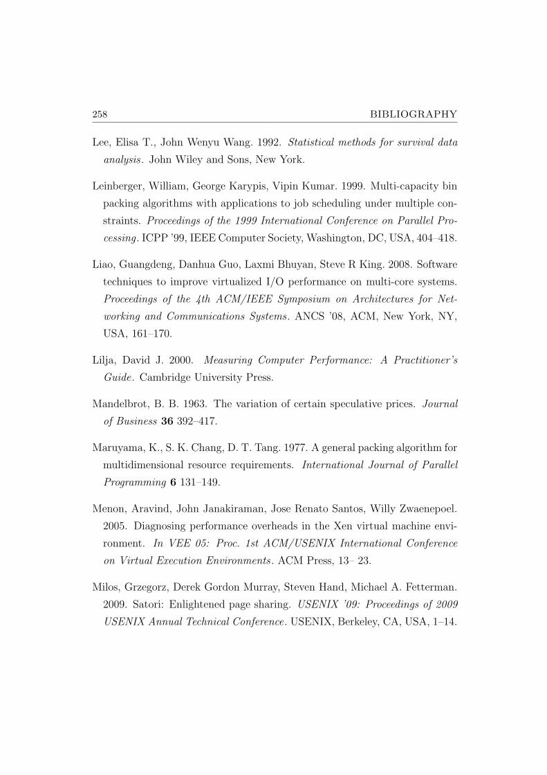
258 BIBLIOGRAPHY
Lee, Elisa T., John Wenyu Wang. 1992. Statistical methods for survival data
analysis . John Wiley and Sons, New York.
Leinberger, William, George Karypis, Vipin Kumar. 1999. Multi-capacity bin
packing algorithms with applications to job scheduling under multiple con-
straints. Proceedings of the 1999 International Conference on Parallel Pro-
cessing . ICPP ’99, IEEE Computer Society, Washington, DC, USA, 404–418.
Liao, Guangdeng, Danhua Guo, Laxmi Bhuyan, Steve R King. 2008. Software
techniques to improve virtualized I/O performance on multi-core systems.
Proceedings of the 4th ACM/IEEE Symposium on Architectures for Net-
working and Communications Systems . ANCS ’08, ACM, New York, NY,
USA, 161–170.
Lilja, David J. 2000. Measuring Computer Performance: A Practitioner’s
Guide. Cambridge University Press.
Mandelbrot, B. B. 1963. The variation of certain speculative prices. Journal
of Business 36 392–417.
Maruyama, K., S. K. Chang, D. T. Tang. 1977. A general packing algorithm for
multidimensional resource requirements. International Journal of Parallel
Programming 6 131–149.
Menon, Aravind, John Janakiraman, Jose Renato Santos, Willy Zwaenepoel.
2005. Diagnosing performance overheads in the Xen virtual machine envi-
ronment. In VEE 05: Proc. 1st ACM/USENIX International Conference
on Virtual Execution Environments . ACM Press, 13– 23.
Milos, Grzegorz, Derek Gordon Murray, Steven Hand, Michael A. Fetterman.
2009. Satori: Enlightened page sharing. USENIX ’09: Proceedings of 2009
USENIX Annual Technical Conference. USENIX, Berkeley, CA, USA, 1–14.
BIBLIOGRAPHY 259
Nathuji, Ripal, Aman Kansal, Alireza Ghaffarkhah. 2010. Q-clouds: managing
performance interference effects for qos-aware clouds. Proceedings of the 5th
European conference on Computer systems . EuroSys ’10, ACM, New York,
NY, USA, 237–250.
Nikolaou, Michael. 2001. Model predictive controllers: A critical synthesis of
theory and industrial needs. Advances in Chemical Engineering , vol. 26.
Academic Press, 131 – 204.
Padala, Pradeep, Kai-Yuan Hou, Kang G. Shin, Xiaoyun Zhu, Mustafa Uysal,
Zhikui Wang, Sharad Singhal, Arif Merchant. 2009. Automated control
of multiple virtualized resources. Proceedings of the 4th ACM European
conference on Computer systems . EuroSys ’09, ACM, New York, NY, USA,
13–26.
Padala, Pradeep, Kang G. Shin, Xiaoyun Zhu, Mustafa Uysal, Zhikui Wang,
Sharad Singhal, Arif Merchant, Kenneth Salem. 2007. Adaptive control of
virtualized resources in utility computing environments. SIGOPS Operating
System Review 41 289–302.
Pu, Xing, Ling Liu, Yiduo Mei, Sankaran Sivathanu, Younggyun Koh, Cal-
ton Pu. 2010. Understanding Performance Interference of I/O Workload in
Virtualized Cloud Environments. IEEE International Conference on Cloud
Computing 51–58.
Rolia, Jerry, Artur Andrzejak, Martin Arlitt. 2003. Automating Enterprise
Application Placement in Resource Utilities. 14th˜IFIP/IEEE˜Workshop on
Distributed Systems:˜Operations and Management (DSOM˜2003), (Work-
shop Theme: ”Self-Managing˜Systems”). Heidelberg, 118–129.
Rolia, Jerry, Xiaoyun Zhu, Martin Arlitt, Artur Andrzejak. 2004. Statistical
service assurances for applications in utility grid environments. Performance
Evaluation 58(2+3) 319–339.
260 BIBLIOGRAPHY
Roy, Nilabja, John S. Kinnebrew, Nishanth Shankaran, Gautam Biswas, Dou-
glas C. Schmidt. 2008. Toward effective multi-capacity resource allocation
in distributed real-time and embedded systems. Proceedings of the 2008
11th IEEE Symposium on Object Oriented Real-Time Distributed Comput-
ing . IEEE Computer Society, Washington, DC, USA, 124–128.
Sapuntzakis, Constantine P., Ramesh Chandra, Ben Pfaff, Jim Chow, Mon-
ica S. Lam, Mendel Rosenblum. 2002. Optimizing the migration of virtual
computers. SIGOPS Operating System Review 36 377–390.
Sargeant, Phil. 2010. Data centre transformation: How mature is your it?
Seiden, Steven S. 2002. On the online bin packing problem. Journal of the
ACM 49 640–671.
Speitkamp, Benjamin, Martin Bichler. 2010. A mathematical programming
approach for server consolidation problems in virtualized data centers. IEEE
Transactions on Services Computing 99(PrePrints).
Stillwell, Mark, David Schanzenbach, Frederic Vivien, Henri Casanova. 2010.
Resource allocation algorithms for virtualized service hosting platforms.
Journal on Parallel Distributed Computing 70 962–974.
Sun Microsystems, Inc. 1995. Nfs version 3 protocol specification. URL http:
//tools.ietf.org/html/rfc1813.
Tam, David, Reza Azimi, Michael Stumm. 2007. Thread clustering: sharing-
aware scheduling on smp-cmp-smt multiprocessors. SIGOPS Operating Sys-
tem Review 41 47–58.
Tam, David K., Reza Azimi, Livio B. Soares, Michael Stumm. 2009. Rapidmrc:
approximating l2 miss rate curves on commodity systems for online opti-
mizations. SIGPLAN Not. 44 121–132.
BIBLIOGRAPHY 261
Tran, Nancy, Daniel A. Reed. 2004. Automatic arima time series modeling for
adaptive i/o prefetching. IEEE Transactions on Parallel Distributed Systems
15 362–377.
Tuck, Nathan, Dean M. Tullsen. 2003. Initial observations of the simultaneous
multithreading pentium 4 processor. Proceedings of the 12th International
Conference on Parallel Architectures and Compilation Techniques . PACT
’03, IEEE Computer Society, Washington, DC, USA, 26–34.
Tullsen, Dean M., Susan J. Eggers, Henry M. Levy. 1998. Simultaneous mul-
tithreading: maximizing on-chip parallelism. 25 years of the international
symposia on Computer architecture (selected papers). ISCA ’98, 533–544.
Urgaonkar, Bhuvan, Prashant Shenoy. 2005. Cataclysm: policing extreme over-
loads in internet applications. Proceedings of the 14th international confer-
ence on World Wide Web. WWW ’05, ACM, New York, NY, USA, 740–749.
doi:10.1145/1060745.1060852.
Urgaonkar, Bhuvan, Prashant Shenoy. 2008. Cataclysm: Scalable overload
policing for internet applications. Journal of Network and Computer Appli-
cations (JNCA) 31 891 – 920.
Urgaonkar, Bhuvan, Prashant Shenoy, Abhishek Chandra, Pawan Goyal, Tim-
othy Wood. 2008. Agile dynamic provisioning of multi-tier internet applica-
tions. ACM Transactions on Autonomic Adaptive Systems 3(1) 1–39.
Urgaonkar, Bhuvan, Prashant Shenoy, Timothy Roscoe. 2009. Resource over-
booking and application profiling in a shared internet hosting platform.
ACM Transactions on Internet Technologies 9(1) 1–45.
van Vliet, Andre. 1992. An improved lower bound for on-line bin packing
algorithms. Information Processing Letters 43 277–284.
262 BIBLIOGRAPHY
Verma, Akshat, Puneet Ahuja, Anindya Neogi. 2008. pmapper: power and
migration cost aware application placement in virtualized systems. Proceed-
ings of the 9th ACM/IFIP/USENIX International Conference on Middle-
ware. Middleware ’08, Springer-Verlag New York, Inc., New York, NY, USA,
243–264.
VMWare. 2012a. Vmware distributed resource scheduler (drs). URL http:
//www.vmware.com/products/drs/overview.html.
VMWare. 2012b. Vmware esxi hypervisor. URL http://www.vmware.com/
products/vsphere/esxi-and-esx/overview.html.
Vogels, Werner. 2008. Beyond server consolidation. ACM Queue 6 20–26.
Waldspurger, Carl A. 2002. Memory resource management in vmware esx
server. SIGOPS Operating System Review 36 181–194.
Wang, Zhikui, Yuan Chen, Daniel Gmach, Sharad Singhal, Brian Watson,
Wilson Rivera, Xiaoyuan Zhu, Chris Hyser. 2009. Appraise: Application-
level performance management in virtualized server environment. IEEE
Transactions on Network and Service Management 6(4) 240 – 254.
Welsh, Matt, David Culler. 2003. Adaptive overload control for busy internet
servers. Proceedings of the 4th conference on USENIX Symposium on Inter-
net Technologies and Systems - Volume 4 . USITS’03, USENIX Association,
Berkeley, CA, USA, 4–14.
Williams, Dan, Hani Jamjoom, Yew-Huey Liu, Hakim Weatherspoon. 2011.
Overdriver: handling memory overload in an oversubscribed cloud. Pro-
ceedings of the 7th ACM SIGPLAN/SIGOPS international conference on
Virtual execution environments . VEE ’11, New York, NY, USA, 205–216.
Williams, David E. 2007. Virtualization with Xen: including XenEnterprise,
XenServer, and XenExpress . Syngress.
BIBLIOGRAPHY 263
Woeginger, Gerhard J. 1997. There is no asymptotic ptas for two-dimensional
vector packing. Information Processing Letters 64(6) 293 – 297.
Wolski, Rich. 1998. Dynamically forecasting network performance using the
network weather service. Cluster Computing 1 119–132.
Wood, Timothy, Ludmila Cherkasova, Kivanc Ozonat, Prashant Shenoy. 2008.
Profiling and modeling resource usage of virtualized applications. Proceed-
ings of the 9th ACM/IFIP/USENIX International Conference on Middle-
ware. Middleware ’08, Springer-Verlag New York, Inc., New York, NY, USA,
366 – 387.
Wood, Timothy, Prashant Shenoy, Arun Venkataramani, Mazin Yousif. 2009a.
Sandpiper: Black-box and gray-box resource management for virtual ma-
chines. Computer Networks 53(17) 2923–2938.
Wood, Timothy, Gabriel Tarasuk-Levin, Prashant Shenoy, Peter Desnoyers,
Emmanuel Cecchet, Mark D. Corner. 2009b. Memory buddies: exploiting
page sharing for smart colocation in virtualized data centers. Proceedings
of the 2009 ACM SIGPLAN/SIGOPS international conference on Virtual
execution environments . VEE ’09, New York, NY, USA, 31–40.
Xu, Wei, Xiaoyun Zhu, S. Singhal, Zhikui Wang. 2006. Predictive control for
dynamic resource allocation in enterprise data centers. Network Operations
and Management Symposium, 2006. NOMS 2006. 10th IEEE/IFIP . 115 –
126.
Yao, Andrew Chi-Chih. 1980. New algorithms for bin packing. Journal of the
ACM 27 207–227.
Zayas, E. 1987. Attacking the process migration bottleneck. SIGOPS Operat-
ing System Review 21 13–24.
264 BIBLIOGRAPHY
Zhang, Qi, Ludmila Cherkasova, Guy Mathews, Wayne Greene, Evgenia
Smirni. 2007. R-capriccio: A capacity planning and anomaly detection tool
for enterprise services with live workloads. Lecture Notes in Computer Sci-
ence, Middleware 2007 4834.
Zhao, Weiming, Zhenlin Wang, Yingwei Luo. 2009. Dynamic memory balanc-
ing for virtual machines. SIGOPS Operating System Review 43 37–47.
Zhou, Fangfei, Manish Goel, Peter Desnoyers, Ravi Sundaram. 2011. Scheduler
vulnerabilities and coordinated attacks in cloud computing. Proceedings of
the 2011 IEEE 10th International Symposium on Network Computing and
Applications . NCA ’11, IEEE Computer Society, Washington, DC, USA,
123–130. doi:10.1109/NCA.2011.24.