Neutrino Oscillation Physics

at

Neutrino Factories and Beta Beams

Mark Benjamin Rolinec

Dissertation

June 2007

Technische Universitat Munchen

Physik-DepartmentInstitut fur Theoretische Physik T30d

Univ.-Prof. Dr. Manfred Lindner

Neutrino Oscillation Physics

at

Neutrino Factories and Beta Beams

Dipl.-Phys. Univ. Mark Benjamin Rolinec

Vollstandiger Abdruck der von der Fakultat fur Physik der Technischen Universitat Munchenzur Erlangung des akademischen Grades eines

Doktors der Naturwissenschaften (Dr. rer. nat.)

genehmigten Dissertation.

Vorsitzender: Univ.-Prof. Dr. Lothar Oberauer

Prufer der Dissertation: 1. Univ.-Prof. Dr. Manfred Lindner

2. Univ.-Prof. Dr. Andrzej J. Buras

Die Dissertation wurde am 13. Juni 2007 bei der Technischen Universitat Munchen eingereichtund durch die Fakultat fur Physik am 23. Juli 2007 angenommen.

Wenn wir jetzt Schinken hatten, konnten wir Ruhrei mitSchinken machen, wenn wir Eier hatten.

Kathrin PassigSie befinden sich hier

I

Contents

1 Introduction 1

2 The Standard Model 5

3 Neutrino Masses and Mixing 9

3.1 Neutrino Mass Terms . . . . . . . . . . . . . . . . . . . . . . . . . . . . . . . . 9

3.2 Neutrino Mixing . . . . . . . . . . . . . . . . . . . . . . . . . . . . . . . . . . . 10

3.3 See-Saw Mechanism . . . . . . . . . . . . . . . . . . . . . . . . . . . . . . . . . 12

3.4 Implications . . . . . . . . . . . . . . . . . . . . . . . . . . . . . . . . . . . . . . 14

4 Neutrino Oscillations 21

4.1 Two Flavor Oscillations . . . . . . . . . . . . . . . . . . . . . . . . . . . . . . . 21

4.2 Matter Effects . . . . . . . . . . . . . . . . . . . . . . . . . . . . . . . . . . . . . 23

4.3 Three Flavor Oscillations . . . . . . . . . . . . . . . . . . . . . . . . . . . . . . 29

4.4 Phenomenology of Peµ and Pee . . . . . . . . . . . . . . . . . . . . . . . . . . . 31

5 Neutrino Data 37

5.1 Number of Flavors . . . . . . . . . . . . . . . . . . . . . . . . . . . . . . . . . . 37

5.2 Absolute Mass Scale . . . . . . . . . . . . . . . . . . . . . . . . . . . . . . . . . 38

5.3 Oscillation Data . . . . . . . . . . . . . . . . . . . . . . . . . . . . . . . . . . . 42

6 Long Baseline Experiment Scenarios 49

6.1 Conventional Beam Experiments . . . . . . . . . . . . . . . . . . . . . . . . . . 50

6.2 Superbeams . . . . . . . . . . . . . . . . . . . . . . . . . . . . . . . . . . . . . . 51

6.3 Reactor Experiments . . . . . . . . . . . . . . . . . . . . . . . . . . . . . . . . . 52

6.4 Electron Capture Beams . . . . . . . . . . . . . . . . . . . . . . . . . . . . . . . 53

6.5 Beta Beams . . . . . . . . . . . . . . . . . . . . . . . . . . . . . . . . . . . . . . 54

6.6 Neutrino Factories . . . . . . . . . . . . . . . . . . . . . . . . . . . . . . . . . . 58

7 Beta Beam Performance 63

7.1 Beta Beam Simulation . . . . . . . . . . . . . . . . . . . . . . . . . . . . . . . . 63

7.2 Beta Beam Optimization . . . . . . . . . . . . . . . . . . . . . . . . . . . . . . . 68

7.3 Neutrino and Anti-Neutrino Runtime Fraction . . . . . . . . . . . . . . . . . . 81

7.4 Addition of T2K Disappearance Data . . . . . . . . . . . . . . . . . . . . . . . . 82

7.5 γ-Scaling of the Isotope Decays . . . . . . . . . . . . . . . . . . . . . . . . . . . 84

7.6 Performance of the β-Beam Reference Scenarios . . . . . . . . . . . . . . . . . . 86

II CONTENTS

8 Neutrino Factory Performance 898.1 Neutrino Factory Simulation . . . . . . . . . . . . . . . . . . . . . . . . . . . . 898.2 Neutrino Factory Optimization . . . . . . . . . . . . . . . . . . . . . . . . . . . 948.3 Neutrino and Anti-Neutrino Runtime Fraction . . . . . . . . . . . . . . . . . . 1008.4 Matter Density Uncertainty . . . . . . . . . . . . . . . . . . . . . . . . . . . . . 1028.5 Inclusion of Different Channels . . . . . . . . . . . . . . . . . . . . . . . . . . . 1038.6 Performance of the Neutrino Factory Reference Scenarios . . . . . . . . . . . . . 108

9 The Global Picture 1139.1 The Road Map of Neutrino Oscillation Experiments . . . . . . . . . . . . . . . 1139.2 Promising Future Experiments . . . . . . . . . . . . . . . . . . . . . . . . . . . 115

10 Summary and Conclusions 121

A The General Long Baseline Experiment Simulator 125

B Performance Indicators 127

Acknowledgments 129

Bibliography 132

III

List of Figures

3.1 Diagramatic illustration of the generation of mL through the See-Saw mechanism. 14

3.2 Mass spectrum of the three neutrino mass eigenstates ν1, ν2, and ν3 for normaland inverted hierarchy. . . . . . . . . . . . . . . . . . . . . . . . . . . . . . . . . 16

3.3 The diagram of the simplest process leading to neutrino-less double beta decay. 17

3.4 The diagram, leading to an effective Majorana mass in case of a black boxprocess for neutrino-less double beta decay. . . . . . . . . . . . . . . . . . . . . 18

3.5 The effective neutrino mass parameter 〈mee〉 relevant for neutrino-less doublebeta decay as a function of the lightest neutrino mass. . . . . . . . . . . . . . . 19

3.6 The tree level and one-loop level Feynman diagrams for the decay of heavyright-handed neutrinos Ni into the Higgs doublet and the lepton doublet, rel-evant for Leptogenesis. . . . . . . . . . . . . . . . . . . . . . . . . . . . . . . . . 20

4.1 Neutrino oscillation probability in the two-flavor scenario as a function of thebaseline and the neutrino energy. . . . . . . . . . . . . . . . . . . . . . . . . . . 22

4.2 The Feynman diagrams for coherent forward scattering of neutrinos in matter . 23

4.3 The Neutrino mixing angle in matter for neutrinos involving the Mikheyev-Smirnov-Wolfenstein resonance and for anti-neutrinos as a function of the mat-ter potential parameter A′. . . . . . . . . . . . . . . . . . . . . . . . . . . . . . 27

4.4 The effective energy eigenvalues in matter and the mass eigenstate compositionof the flavor eigenstate |να〉 as functions of the matter potential parameter A′. . 29

5.1 Possible neutrino mass spectra with a fourth sterile neutrino and an additionalmass-squared difference ∆m2

LSND. . . . . . . . . . . . . . . . . . . . . . . . . . . 47

6.1 Schematic illustration of neutrino source, oscillation channels, and detectionprinciples at conventional beam experiments and at Superbeam experiments. . 51

6.2 Schematic illustration of neutrino source, oscillation channels, and detectionprinciples at a neutrino reactor experiment. . . . . . . . . . . . . . . . . . . . . 53

6.3 Schematic illustration of neutrino source, oscillation channels, and detectionprinciples at a β-Beam experiment. . . . . . . . . . . . . . . . . . . . . . . . . . 56

6.4 The energy spectrum of the neutrino flux at a β-Beam experiment. . . . . . . . 57

6.5 Schematic illustration of neutrino source, oscillation channels, and detectionprinciples at a Neutrino Factory experiment. . . . . . . . . . . . . . . . . . . . 59

6.6 The energy spectrum of the neutrino flux at a Neutrino Factory experiment. . . 60

7.1 The sensitivity limit to sin2 2θ13 at a β-Beam (WC) as a function of the baselineL at fixed γ = 150 and γ = 350. . . . . . . . . . . . . . . . . . . . . . . . . . . . 69

IV LIST OF FIGURES

7.2 The sensitivity limit to sin2 2θ13 at a β-Beam (TASD) as a function of thebaseline L at fixed γ = 500 and γ = 1000. . . . . . . . . . . . . . . . . . . . . . 70

7.3 The sensitivity limit to sin2 2θ13 at a β-Beam (WC) as a function of γ at thefixed baselines L = 130 km and L = 730 km. . . . . . . . . . . . . . . . . . . . 71

7.4 The sensitivity limit to sin2 2θ13 at a β-Beam (TASD) as a function of γ at thefixed baselines L = 730 km and L = 1500 km. . . . . . . . . . . . . . . . . . . . 73

7.5 The sensitivity to maximal CP violation at a β-Beam as a function of thebaseline L at fixed a γ. . . . . . . . . . . . . . . . . . . . . . . . . . . . . . . . . 74

7.6 The sensitivity to maximal CP violation at a β-Beam as a function of γ at afixed baseline L. . . . . . . . . . . . . . . . . . . . . . . . . . . . . . . . . . . . 75

7.7 The sensitivity to mass hierarchy at a β-Beam as a function of the baseline Lat fixed γ. . . . . . . . . . . . . . . . . . . . . . . . . . . . . . . . . . . . . . . . 77

7.8 The sensitivity to mass hierarchy at a β-Beam as a function of γ at a fixedbaseline L. . . . . . . . . . . . . . . . . . . . . . . . . . . . . . . . . . . . . . . . 79

7.9 The impact of the ratio of neutrino (18Ne stored) and anti-neutrino (6Hestored) runtime at a β-Beam on the sensitivity limit to sin2 2θ13, the sensitivityto maximal CP violation, and sensitivity to the mass hierarchy. . . . . . . . . . 81

7.10 The impact of the addition of T2K disappearance data to the β-Beam data onthe sin2 2θ13 discovery reach, the sensitivity to any CP violation, and sensitivityto the mass hierarchy. . . . . . . . . . . . . . . . . . . . . . . . . . . . . . . . . 83

7.11 The impact of the γ-scaling of the number of isotope decays per year at a β-Beam on the sin2 2θ13 discovery reach, the sensitivity to any CP violation, andsensitivity to the mass hierarchy. . . . . . . . . . . . . . . . . . . . . . . . . . . 85

7.12 The comparison of the performance of all β-Beam reference scenarios for theperformance indicators sin2 2θ13 discovery reach, sensitivity to any CP viola-tion, and sensitivity to the mass hierarchy. . . . . . . . . . . . . . . . . . . . . . 87

8.1 The sensitivity limit to sin2 2θ13 at a Neutrino Factory as a function of thebaseline L for a fixed parent muon energy of Eµ = 25 GeV and Eµ = 50 GeV. . 95

8.2 The sensitivity limit to sin2 2θ13 at a Neutrino Factory as a function of theparent muon energy for a fixed baseline of L = 4000 km and L = 7500 km. . 96

8.3 The sensitivity to maximal CP violation at a Neutrino Factory as a function ofthe baseline L for a fixed parent muon energies of Eµ = 25 GeV and Eµ = 50 GeV. 97

8.4 The sensitivity to mass hierarchy at a Neutrino Factory as a function of thebaseline L for a fixed parent muon energies of Eµ = 25 GeV and Eµ = 50 GeV. 98

8.5 The impact of the ratio of neutrino and anti-neutrino runtime at a NeutrinoFactory on the sensitivity limit to sin2 2θ13, the sensitivity to maximal CPviolation, and sensitivity to the mass hierarchy. . . . . . . . . . . . . . . . . . . 101

8.6 The impact of the matter density uncertainty at a Neutrino Factory on thesin2 2θ13 discovery reach, the sensitivity to any CP violation, and sensitivity tothe mass hierarchy. . . . . . . . . . . . . . . . . . . . . . . . . . . . . . . . . . . 103

8.7 The sensitivity gap coverage for a combination of golden and silver channel asa function of the silver channel detector . . . . . . . . . . . . . . . . . . . . . . 105

8.8 The impact of the upper platinum CID threshold to the CP violation sensitivityfor small, intermediate, and large sin2 2θ13. . . . . . . . . . . . . . . . . . . . . 106

LIST OF FIGURES V

8.9 The comparison of the improvement of the standard and optimistic silver andplatinum channel scenarios considering CP violation and mass hierarchy sensi-tivity for large and intermediate sin2 2θ13. . . . . . . . . . . . . . . . . . . . . . 108

8.10 The comparison of the performance of all Neutrino Factory reference scenariosfor the performance indicators sin2 2θ13 discovery reach, sensitivity to any CPviolation, and sensitivity to the mass hierarchy. . . . . . . . . . . . . . . . . . . 110

9.1 Possible global evolution of the sin2 2θ13 discovery reach as a function of time. . 1149.2 Summary of the performances of all β-Beam and Neutrino Factory reference

scenarios for the performance indicators sin2 2θ13 discovery, sensitivity to anyCP violation, and sensitivity to the mass hierarchy at the true value sin2 2θ13 =10−1. . . . . . . . . . . . . . . . . . . . . . . . . . . . . . . . . . . . . . . . . . . 116

9.3 Summary of the performances of all β-Beam and Neutrino Factory referencescenarios for the performance indicators sin2 2θ13 discovery, sensitivity to anyCP violation, and sensitivity to the mass hierarchy at the true value sin2 2θ13 =10−3. . . . . . . . . . . . . . . . . . . . . . . . . . . . . . . . . . . . . . . . . . . 118

9.4 Summary of the performances of all β-Beam and Neutrino Factory reference sce-narios for the sin2 2θ13 reach of the performance indicators sin2 2θ13 discovery,sensitivity to any CP violation, and sensitivity to the mass hierarchy. . . . . . . 119

VI LIST OF FIGURES

VII

List of Tables

2.1 The fermion particle content of the Standard Model. . . . . . . . . . . . . . . . 62.2 The Higgs scalar field of the Standard Model . . . . . . . . . . . . . . . . . . . 7

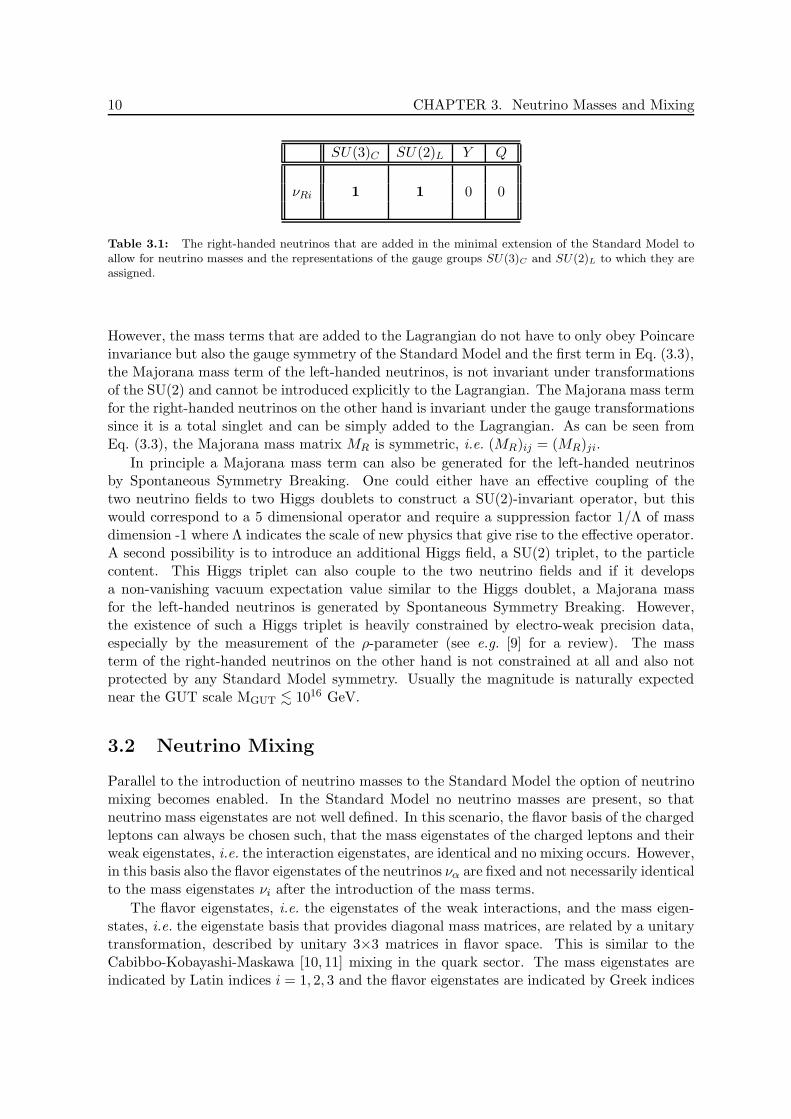
3.1 The right-handed neutrinos that are added in the minimal extension of theStandard Model to allow for neutrino masses. . . . . . . . . . . . . . . . . . . . 10

7.1 The signal efficiencies and background rejection factors and systematical errorsin our description of the Water Cherenkov detector β-Beams. . . . . . . . . . . 66

7.2 The signal efficiencies and background rejection factors and systematical errorsin our description of the Totally Active Scintillator detector β-Beams. . . . . . 67

7.3 The listing of all defined β-Beam reference scenarios. . . . . . . . . . . . . . . . 80

8.1 The signal efficiencies and background rejection factors and systematical errorsin our description of the standard golden channel at a Neutrino Factory. . . . . 90

8.2 The signal efficiencies and background rejection factors and systematical errorsin our description of the standard silver channel at a Neutrino Factory. . . . . . 91

8.3 The signal efficiencies and background rejection factors and systematical errorsin our description of the standard platinum channel at a Neutrino Factory. . . . 92

8.4 The listing of all defined Neutrino Factory reference scenarios. . . . . . . . . . . 100

VIII LIST OF TABLES

1

Chapter 1

Introduction

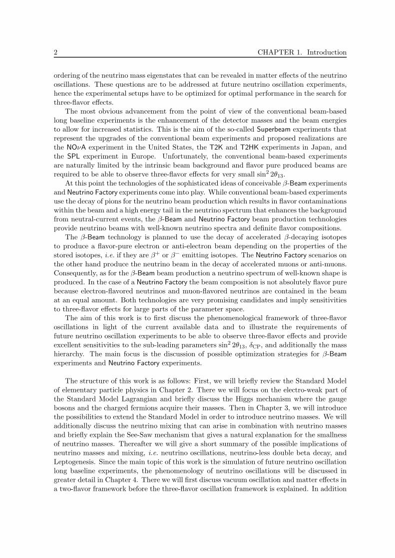
Neutrino oscillation physics has clearly entered the era of beam-based long baseline experi-ments. Already a few years ago in 2002, the first experiment, the K2K in Japan, that usesa collimated νµ neutrino beam to search for oscillations at the atmospheric frequency, hasconfirmed the oscillations that have been observed in data coming from atmospheric neutri-nos. At this time the succeeding conventional beam-based neutrinos oscillation long baselineexperiments were in the stage of preparation, the MINOS experiment in the United states andthe CNGS experiments in Europe.

In 2006 the MINOS collaboration published their highly anticipated results of the first yearof operation which was in perfect agreement with the data from atmospheric neutrinos andK2K. Additionally, the MINOS results could already significantly improve the precision in themeasurement of the atmospheric parameter |∆m2

31|. This amazing development followed theextraordinary example of the KamLAND experiment in Japan, where in 2003 the data froma totally earth-based experiment could confirm and even improve the measurements fromnaturally produced neutrinos, i.e. in case of KamLAND the data from solar neutrinos.

Recently, also the CNGS beam delivered the first neutrinos which then could be detectedin the Gran Sasso underground laboratories in Italy at the OPERA detector after travelingalong the 732 km baseline from their production at CERN in Switzerland. Now, all threebeam-based neutrino oscillation long baseline experiment setups are in operation.

However, the first generation of conventional beam-based neutrino oscillation long baselineexperiments will mainly contribute to the precision measurements of the leading atmosphericparameters since the experiments do not provide good sensitivities to three-flavor effectsbecause of the relatively small detector dimensions and the relatively small beam powerscompared to planned future experiment scenarios. The reason is that three-flavor effects,which would manifest in the appearance of electron neutrinos from the muon neutrino beamsat the conventional beam-based oscillation experiments, are suppressed due to the small thirdmixing angle sin2 2θ13 and the hierarchy of the oscillation frequencies ∆m2

21/∆m231, resulting

in an effective decoupling of the atmospheric and solar neutrino oscillations that are so farwell explained in an effective two-flavor picture.

It is the goal of future neutrino oscillation experiments to discover three-flavor effectsbeyond the pure precision measurements of the leading oscillation parameters and variouslong baseline scenarios have been proposed to shed light on the puzzles of three-flavor oscil-lations, i.e. the question of the actual size of the small mixing angle sin2 2θ13, the questionof the presence of CP violation in the neutrino sector, and the question of the actual mass

2 CHAPTER 1. Introduction

ordering of the neutrino mass eigenstates that can be revealed in matter effects of the neutrinooscillations. These questions are to be addressed at future neutrino oscillation experiments,hence the experimental setups have to be optimized for optimal performance in the search forthree-flavor effects.

The most obvious advancement from the point of view of the conventional beam-basedlong baseline experiments is the enhancement of the detector masses and the beam energiesto allow for increased statistics. This is the aim of the so-called Superbeam experiments thatrepresent the upgrades of the conventional beam experiments and proposed realizations arethe NOνA experiment in the United States, the T2K and T2HK experiments in Japan, andthe SPL experiment in Europe. Unfortunately, the conventional beam-based experimentsare naturally limited by the intrinsic beam background and flavor pure produced beams arerequired to be able to observe three-flavor effects for very small sin2 2θ13.

At this point the technologies of the sophisticated ideas of conceivable β-Beam experimentsand Neutrino Factory experiments come into play. While conventional beam-based experimentsuse the decay of pions for the neutrino beam production which results in flavor contaminationswithin the beam and a high energy tail in the neutrino spectrum that enhances the backgroundfrom neutral-current events, the β-Beam and Neutrino Factory beam production technologiesprovide neutrino beams with well-known neutrino spectra and definite flavor compositions.

The β-Beam technology is planned to use the decay of accelerated β-decaying isotopesto produce a flavor-pure electron or anti-electron beam depending on the properties of thestored isotopes, i.e. if they are β+ or β− emitting isotopes. The Neutrino Factory scenarios onthe other hand produce the neutrino beam in the decay of accelerated muons or anti-muons.Consequently, as for the β-Beam beam production a neutrino spectrum of well-known shape isproduced. In the case of a Neutrino Factory the beam composition is not absolutely flavor purebecause electron-flavored neutrinos and muon-flavored neutrinos are contained in the beamat an equal amount. Both technologies are very promising candidates and imply sensitivitiesto three-flavor effects for large parts of the parameter space.

The aim of this work is to first discuss the phenomenological framework of three-flavoroscillations in light of the current available data and to illustrate the requirements offuture neutrino oscillation experiments to be able to observe three-flavor effects and provideexcellent sensitivities to the sub-leading parameters sin2 2θ13, δCP, and additionally the masshierarchy. The main focus is the discussion of possible optimization strategies for β-Beamexperiments and Neutrino Factory experiments.

The structure of this work is as follows: First, we will briefly review the Standard Modelof elementary particle physics in Chapter 2. There we will focus on the electro-weak part ofthe Standard Model Lagrangian and briefly discuss the Higgs mechanism where the gaugebosons and the charged fermions acquire their masses. Then in Chapter 3, we will introducethe possibilities to extend the Standard Model in order to introduce neutrino masses. We willadditionally discuss the neutrino mixing that can arise in combination with neutrino massesand briefly explain the See-Saw mechanism that gives a natural explanation for the smallnessof neutrino masses. Thereafter we will give a short summary of the possible implications ofneutrino masses and mixing, i.e. neutrino oscillations, neutrino-less double beta decay, andLeptogenesis. Since the main topic of this work is the simulation of future neutrino oscillationlong baseline experiments, the phenomenology of neutrino oscillations will be discussed ingreater detail in Chapter 4. There we will first discuss vacuum oscillation and matter effects ina two-flavor framework before the three-flavor oscillation framework is explained. In addition

CHAPTER 1. Introduction 3

we will discuss expansions of the three-flavor oscillation probabilities of the relevant channelsthat are later discussed for the respective experiments. This discussion will set an analyticalbasis that allows to understand the numeric results that are discussed in later chapters.

In Chapter 5 the current available neutrino data and the current knowledge about neutrinoproperties will be presented. This involves a discussion of data that allows a conclusion aboutthe number of neutrino flavors, data that allows constraining the absolute mass scale ofneutrinos, and finally the available oscillation data. The latter will be discussed in regard tothe data from solar neutrinos, atmospheric neutrinos, and artificially produced neutrinos inreactor cores or in pion decays for the first generation of conventional beam-based experiments.There we will also briefly discuss the results from the neutrino experiment LSND that do notagree with the global data in the three-flavor framework. The next Chapter will give a detaileddescription of the technologies of proposed or conceivable future neutrino oscillation longbaseline experiments, i.e. the conventional accelerator beam-based experiments, their possibleupgrades, the so-called Superbeam scenarios, reactor experiments, neutrino experiments witha neutrino beam from electron capture, and of course the experiment technologies that willbe simulated in the chapters where the main results are presented: β-Beam experiments andNeutrino Factory experiments.

In Chapter 7 we will give a detailed discussion of the performance of β-Beam experimentswhere we focus on different detector technologies, Water Cherenkov and Totally Active Scin-tillator, and the three basic categories of β-Beam experiments: low γ, medium γ, and highγ. First the details of the simulation techniques are presented before we give an extensivediscussion of the β-Beam optimization in terms of the baseline L and the acceleration factor γof the stored isotopes. Thereafter, we will concentrate on single technical considerations suchas the impact of the ratio of the neutrino and anti-neutrino runtime fractions, the impact ofexternal disappearance data to handle parameter correlations with the leading atmosphericoscillation parameters, and the impact of a possible γ-scaling of the number of isotope decaysthat affects the potential of medium and high γ scenarios. Finally, we will compare the per-formances of optimized β-Beam reference scenarios for both detector technologies in terms ofthe performance indicators: discovery reach in sin2 2θ13, sensitivity to any CP violation, andsensitivity to the mass hierarchy.

Thereafter in Chapter 8 the main focus will lie on the performance of Neutrino Factoryscenarios at very large baselines. Again, we will first introduce the simulation techniques forthe Neutrino Factory simulations. Then, as for the β-Beams in the previous chapter a detaileddiscussion considering the optimization of a golden channel Neutrino Factory experiment interms of the baseline L and the energy of the stored parent muons Eµ will be presented.Also for the Neutrino Factory experiments we will examine technical considerations such asthe impact of the ratio of the runtime fractions in the µ+-stored and the µ−-stored phase,the impact of the matter density uncertainty along the baseline, and the impact of additionalchannels: the silver channel νe → ντ and the platinum channel νµ → νe. Finally, we willcompare the performances of optimized Neutrino Factory reference scenarios including theadditional channel scenarios, multiple detector scenarios, and an optimized golden channelscenario with a lower threshold and better energy resolution in terms of the performanceindicators: discovery reach in sin2 2θ13, sensitivity to any CP violation, and sensitivity to themass hierarchy.

The performance of the optimized reference scenarios, the different β-Beam scenarios fromChapter 7 and the different Neutrino Factory scenarios from Chapter 8 will be compared inChapter 9 for different regions of true sin2 2θ13. The aim is to find the optimal technology

4 CHAPTER 1. Introduction

in the respective regimes of sin2 2θ13 and to discuss the advantages and disadvantages of thedifferent setups. In this Chapter we will also give a discussion of the future road map of futureneutrino oscillation experiments of various technologies and expenses in order to classify theβ-Beam and Neutrino Factory performances before we give the summary and conclusions.

5

Chapter 2

The Standard Model

The Standard Model of elementary particle physics describes the interactions of all knownelementary particles very successfully up to the high energies at the electroweak scale. Theformulation of the electro-weak interactions within the Standard Model goes back to the1960’s [1–3] and the extension including the strong interactions went on to the 1970’s [4]. Themodel has been tested to very accurate precisions and no deviations have been found at theexperiments of the collider facilities LEP or Tevatron. Three of the four known fundamentalinteractions are combined into one theory, the strong interactions of the quarks, the weakinteractions of leptons and quarks, and the electromagnetic interactions of charged particles.Only the gravitational force is not included to the Standard Model, but the gravitationalinteractions are the weakest of the four fundamental forces at the observable energies andthus negligible. However, it is expected that at very high energies, i.e. the Planck ScaleMP l ∼ 1019GeV, the gravitational forces become similarly significant. This is the firstindication that, despite the extreme success of the Standard Model, it can only be seenas an effective theory at the observable energies and physics at higher energies has to beexpected. Further reasons to believe in new physics beyond the Standard Model are theHierarchy Problem, i.e. the question of stabilization of the Higgs mass against quadraticdivergencies, or the puzzles of the origin of Dark Matter and Dark Energy. The evidencefor neutrino masses that has been established with the observation of neutrino oscillations isalso considered as a hint for physics beyond the Standard Model.

The Standard Model is a local gauge theory with the underlying local gauge symmetry of thegroup

GSM = SU(3)C × SU(2)L × U(1)Y , (2.1)

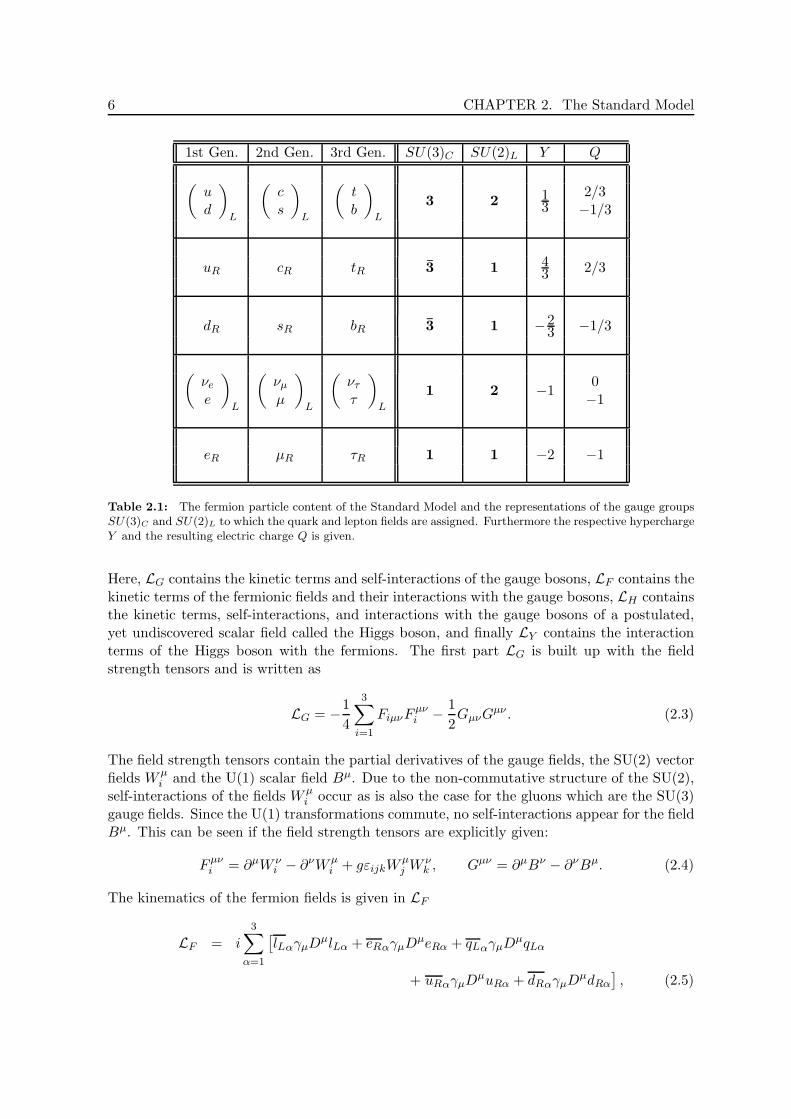
where the strong interactions are associated with the local SU(3) symmetry. The unifiedelectro-weak interactions are governed by the SU(2)×U(1) and only the left-handed compo-nents of the fermion fields transform under the SU(2) group, hence the right-handed com-ponents do not participate in the weak interactions. The particle content of the StandardModel and the associated representations of the Standard Model gauge group are summarizedin Table 2.1. We will here only focus on the electro-weak part of the Standard Model sincethe strong interactions are not relevant for the considerations of this work. The electro-weakinteractions are described in the electro-weak part of the Standard Model Lagrangian

LSU(2)L×U(1)Y= LG + LF + LH + LY . (2.2)

6 CHAPTER 2. The Standard Model

1st Gen. 2nd Gen. 3rd Gen. SU(3)C SU(2)L Y Q

(ud

)

L

(cs

)

L

(tb

)

L

3 2 13

2/3−1/3

uR cR tR 3 1 43 2/3

dR sR bR 3 1 −23 −1/3

(νe

e

)

L

(νµ

µ

)

L

(ντ

τ

)

L

1 2 −10−1

eR µR τR 1 1 −2 −1

Table 2.1: The fermion particle content of the Standard Model and the representations of the gauge groupsSU(3)C and SU(2)L to which the quark and lepton fields are assigned. Furthermore the respective hyperchargeY and the resulting electric charge Q is given.

Here, LG contains the kinetic terms and self-interactions of the gauge bosons, LF contains thekinetic terms of the fermionic fields and their interactions with the gauge bosons, LH containsthe kinetic terms, self-interactions, and interactions with the gauge bosons of a postulated,yet undiscovered scalar field called the Higgs boson, and finally LY contains the interactionterms of the Higgs boson with the fermions. The first part LG is built up with the fieldstrength tensors and is written as

LG = −1

4

3∑

i=1

FiµνFµνi − 1

2GµνGµν . (2.3)

The field strength tensors contain the partial derivatives of the gauge fields, the SU(2) vectorfields W µ

i and the U(1) scalar field Bµ. Due to the non-commutative structure of the SU(2),self-interactions of the fields W µ

i occur as is also the case for the gluons which are the SU(3)gauge fields. Since the U(1) transformations commute, no self-interactions appear for the fieldBµ. This can be seen if the field strength tensors are explicitly given:

Fµνi = ∂µW ν

i − ∂νW µi + gεijkW

µj W ν

k , Gµν = ∂µBν − ∂νBµ. (2.4)

The kinematics of the fermion fields is given in LF

LF = i3∑

α=1

[lLαγµDµlLα + eRαγµDµeRα + qLαγµDµqLα

+ uRαγµDµuRα + dRαγµDµdRα

], (2.5)

CHAPTER 2. The Standard Model 7

Higgs SU(3)C SU(2)L Y Q

φ =

(φ+

φ0

)

1 2 110

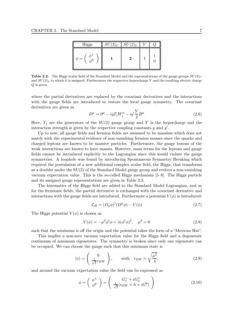
Table 2.2: The Higgs scalar field of the Standard Model and the representations of the gauge groups SU(3)C

and SU(2)L to which it is assigned. Furthermore the respective hypercharge Y and the resulting electric chargeQ is given.

where the partial derivatives are replaced by the covariant derivatives and the interactionswith the gauge fields are introduced to restore the local gauge symmetry. The covariantderivatives are given as

Dµ = ∂µ − igTjWµj − ig′

Y

2Bµ (2.6)

Here, Tj are the generators of the SU(2) gauge group and Y is the hypercharge and theinteraction strength is given by the respective coupling constants g and g′.

Up to now, all gauge fields and fermion fields are assumed to be massless which does notmatch with the experimental evidence of non-vanishing fermion masses since the quarks andcharged leptons are known to be massive particles. Furthermore, the gauge bosons of theweak interactions are known to have masses. However, mass terms for the leptons and gaugefields cannot be introduced explicitly to the Lagrangian since this would violate the gaugesymmetries. A loophole was found by introducing Spontaneous Symmetry Breaking whichrequired the postulation of a new additional complex scalar field, the Higgs, that transformsas a doublet under the SU(2) of the Standard Model gauge group and evolves a non-vanishingvacuum expectation value. This is the so-called Higgs mechanism [5–8]. The Higgs particleand its assigned gauge representations are given in Table 2.2.

The kinematics of the Higgs field are added to the Standard Model Lagrangian, and asfor the fermionic fields, the partial derivative is exchanged with the covariant derivative andinteractions with the gauge fields are introduced. Furthermore a potential V (φ) is introduced:

LH = (Dµφ)†(Dµφ) − V (φ) (2.7)

The Higgs potential V (φ) is chosen as

V (φ) = −µ2φ†φ + λ(φ†φ)2, µ2 > 0 (2.8)

such that the minimum is off the origin and the potential takes the form of a “Mexican Hat”.This implies a non-zero vacuum expectation value for the Higgs field and a degenerate

continuum of minimum eigenstates. The symmetry is broken since only one eigenstate canbe occupied. We can choose the gauge such that this minimum state is

〈φ〉 =

(

01√2vEW

)

, with vEW =

√

µ2

λ. (2.9)

and around the vacuum expectation value the field can be expressed as

φ =

(φ+

φ0

)

=

(

G+1 + iG+

21√2(vEW + h + iG0)

)

(2.10)

8 CHAPTER 2. The Standard Model

where the Goldstone bosons G+1 , G+

2 , and G0 get “eaten” by inserting this into the Lagrangianand introducing the following linear combinations of the gauge fields:

W±µ =

1√2(W 1

µ ∓ W 2µ)

Zµ = cos(θW )W 3µ − sin(θW )Bµ

Aµ = cos(θW )Bµ + sin(θW )W 3µ . (2.11)

Here, we already introduced the Weinberg angle θW that is defined as

cos(θW ) =g

√

g2 + g′2, sin(θW ) =

g′√

g2 + g′2. (2.12)

Furthermore, the gauge bosons aquire masses due to the non-vanishing vacuum expectationvalue vEW because the Higgs part LH of the Lagrangian contains the following terms afterSpontaneous Symmetry Breaking that can be interpreted as mass terms

LH ⊃ 1

8v2EW (g2 + g′2)ZµZµ +

1

4v2EW g2W−

µ W+µ =1

2m2

ZZµZµ + m2W W−

µ W+µ (2.13)

and as can be seen, the masses of the W and the Z bosons are related by the Weinberg angle.The Higgs mechanism additionally allows to introduce masses for the fermions by adding

the so-called Yukawa interactions of the Higgs field with the quark and charged lepton fieldsto the Lagrangian:

LY = −3∑

α,β=1

[(Yl)αβ lLαφeRβ + (Yd)αβqLαφdRβ + (Yu)αβqLα(iσ2φ

∗)uRβ

]+ h.c. (2.14)

Here, the Yukawa couplings Yl, Yd, and Yu are 3×3 matrices in flavor space. If one now con-siders Spontaneous Symmetry Breaking, the fermions aquire masses due to the non-vanishingvacuum expectation value similar to the gauge bosons:

LYSSB−→ −

3∑

α,β=1

[(Ml)αβeLαeRβ + (Md)αβdLαdRβ + (Mu)αβuLαuRβ

]+ h.c. (2.15)

where the mass matrices are given by

Mu =1√2vEW Yu, Md =

1√2vEW Yd, Ml =

1√2vEW Yl. (2.16)

Note, that the neutrinos cannot acquire masses in the Standard Model since right-handedneutrinos νR are not contained in the Standard Model particle content. These right-handedneutrinos would carry no charge or hypercharge and be singlets under SU(2) and SU(3), hencethey would be absolute singlets under the Standard Model gauge transformations and do notinteract with any of the Standard Model particles. So, they have not been introduced andneutrinos were believed to be massless particles.

However, the observations of the last decade have established flavor transitions in theneutrino sector and neutrinos have been observed to be massive. So, the Standard Model ofelementary particle physics has to be extended in order to allow for neutrino masses.

9

Chapter 3

Neutrino Masses and Mixing

Within the last Chapter, we briefly discussed the electro-weak part of the Standard Modeland the Higgs mechanism where the gauge bosons of the weak interactions and the fermionsacquire a mass. It was stated that no masses have been assigned to the neutrinos in thismechanism since no right-handed neutrinos have been introduced to the particle content ofthe Standard Model. However, the experimental evidence of neutrino oscillations indicatesthat neutrinos indeed have masses. This requires an extension of the Standard Model andneutrino masses have to be introduced.

3.1 Neutrino Mass Terms

The simplest extension of the Standard Model to incorporate neutrino masses is to introduceright-handed neutrinos to the particle content. These are singlets under the SU(3) and theSU(2). Furthermore neutrinos do not carry electric charge and hence also no Hypercharge asis summarized in Table 3.1. So, the right-handed neutrinos do not contribute to the electro-weak interactions but similar to the other fermions one can introduce Yukawa couplings to theHiggs field that lead to an additional fermionic Dirac mass term after Spontaneous SymmetryBreaking, now for the neutrinos:

LDiracν = −

∑

α,i

(Yν)αilLα(iσ2φ∗)νRi + h.c.

SSB−→ −∑

α,i

(mD)αiνLανRi + h.c. (3.1)

Again, the Yukawa coupling Yν is a 3×3 matrix in flavor space and the neutrino Dirac massmatrix is given by the Yukawa coupling and the vacuum expectation value of the Higgs field:

mD =1√2vEW Yν (3.2)

Especially for neutrinos, since they do not carry electric charge, there exists a second way tointroduce a Poincare invariant neutrino mass term besides a Dirac type mass term that canbe added to the Lagrangian, a so-called Majorana mass term:

LMajoranaν = −1

2

∑

α,β

(mL)αβνLα(νL)Cβ

︸ ︷︷ ︸

not SU(2)L invariant

−1

2

3∑

i,j=1

(MR)ij(νR)Ci νRj + h.c. (3.3)

10 CHAPTER 3. Neutrino Masses and Mixing

SU(3)C SU(2)L Y Q

νRi 1 1 0 0

Table 3.1: The right-handed neutrinos that are added in the minimal extension of the Standard Model toallow for neutrino masses and the representations of the gauge groups SU(3)C and SU(2)L to which they areassigned.

However, the mass terms that are added to the Lagrangian do not have to only obey Poincareinvariance but also the gauge symmetry of the Standard Model and the first term in Eq. (3.3),the Majorana mass term of the left-handed neutrinos, is not invariant under transformationsof the SU(2) and cannot be introduced explicitly to the Lagrangian. The Majorana mass termfor the right-handed neutrinos on the other hand is invariant under the gauge transformationssince it is a total singlet and can be simply added to the Lagrangian. As can be seen fromEq. (3.3), the Majorana mass matrix MR is symmetric, i.e. (MR)ij = (MR)ji.

In principle a Majorana mass term can also be generated for the left-handed neutrinosby Spontaneous Symmetry Breaking. One could either have an effective coupling of thetwo neutrino fields to two Higgs doublets to construct a SU(2)-invariant operator, but thiswould correspond to a 5 dimensional operator and require a suppression factor 1/Λ of massdimension -1 where Λ indicates the scale of new physics that give rise to the effective operator.A second possibility is to introduce an additional Higgs field, a SU(2) triplet, to the particlecontent. This Higgs triplet can also couple to the two neutrino fields and if it developsa non-vanishing vacuum expectation value similar to the Higgs doublet, a Majorana massfor the left-handed neutrinos is generated by Spontaneous Symmetry Breaking. However,the existence of such a Higgs triplet is heavily constrained by electro-weak precision data,especially by the measurement of the ρ-parameter (see e.g. [9] for a review). The massterm of the right-handed neutrinos on the other hand is not constrained at all and also notprotected by any Standard Model symmetry. Usually the magnitude is naturally expectednear the GUT scale MGUT . 1016 GeV.

3.2 Neutrino Mixing

Parallel to the introduction of neutrino masses to the Standard Model the option of neutrinomixing becomes enabled. In the Standard Model no neutrino masses are present, so thatneutrino mass eigenstates are not well defined. In this scenario, the flavor basis of the chargedleptons can always be chosen such, that the mass eigenstates of the charged leptons and theirweak eigenstates, i.e. the interaction eigenstates, are identical and no mixing occurs. However,in this basis also the flavor eigenstates of the neutrinos να are fixed and not necessarily identicalto the mass eigenstates νi after the introduction of the mass terms.

The flavor eigenstates, i.e. the eigenstates of the weak interactions, and the mass eigen-states, i.e. the eigenstate basis that provides diagonal mass matrices, are related by a unitarytransformation, described by unitary 3×3 matrices in flavor space. This is similar to theCabibbo-Kobayashi-Maskawa [10, 11] mixing in the quark sector. The mass eigenstates areindicated by Latin indices i = 1, 2, 3 and the flavor eigenstates are indicated by Greek indices

3.2 Neutrino Mixing 11

α = e, µ, τ :

eLα =∑

i

(U eL)αi eLi eRα =

∑

i

(U eR)αi eRi

νLα =∑

i

(UνL)αi νLi νRα =

∑

i

(UνR)αi νRi (3.4)

These so defined unitary matrices diagonalize the mass matrices in flavor space, which readsfor the charged leptons as

(U eL)∗αi(Ml)αβ(U e

R)βj = mliδij . (3.5)

For the neutrinos, one has to discriminate between the two possible underlying mass terms,how to diagonalize the mass matrices:

Dirac Neutrino Case : (UνL)∗αi(mD)αβ(Uν

R)βj = mνiδij

Majorana Neutrino Case : (UνL)αi(mL)αβ(Uν

L)βj = mνiδij (3.6)

Now, we will focus on the weak interactions of the neutrinos and see how the lepton mixingaffects the interactions of neutrinos. The relevant part of the Lagrangian is:

LνW = −

∑

α

[g√2eLαγµνLαW−

µ +g

4 cos θνLαγµνLαZ0

µ

]

+ h.c.

= −∑

i,j

[g√2eLi(U

eL)∗αiγ

µ(UνL)αjνLjW

−µ +

g

4 cos θνLi(U

νL)∗αiγ

µ(UνL)αjνLjZ

0µ

]

+ h.c.

= −∑

i,j

[g√2eLiγ

µ(U e†L Uν

L)ijνLjW−µ +

g

4 cos θνLiγ

µνLiZ0µ

]

+ h.c. (3.7)

As can be seen, the unitary matrices cancel out in case of neutral current interaction ofthe neutrinos due to the unitarity condition. The charged current interactions however aresensitive to leptonic mixing, since the mixing matrices do not cancel. In general, one considersa flavor basis, where the charged lepton eigenstates do correspond to their mass eigenstatesand leptonic mixing is shifted to the neutrino sector. In this case only one unitary matrix Umerges the mixing of the leptonic sector:

U = U e†L Uν

L (3.8)

The unitary matrix U is the mixing matrix of neutrinos, sometimes referred to as thePontecorvo-Maki-Nakagawa-Sakata mixing matrix [12]. Similar to the standard parameter-ization of the Cabibbo-Kobayashi-Maskawa matrix in the quark sector, the matrix can beparameterized by three Euler angles θ12, θ13, and θ23. Furthermore, U can generally be acomplex matrix and six phases remain as free parameters in the parameterization after thenine unitarity constraints are considered. However, three of these phases are unphysical be-cause they can be canceled out by a re-definition of the charged lepton fields, i.e. these phasesare absorbed. The remaining phases are referred to as the Dirac phase δCP and the Majoranaphases φ1 and φ2. The parameterization has to be defined by the ordering of the three Euler

12 CHAPTER 3. Neutrino Masses and Mixing

rotations matrices U12, U13, and U23:

U23 =

1 0 00 c23 s23

0 −s23 c23

, U13

c13 0 s13e−iδCP

0 1 0−s13e

iδCP 0 c13

U12 =

c12 s12 0−s12 c12 0

0 0 1

, PM =

eiφ1/2 0 0

0 eiφ2/2 00 0 1

(3.9)

Here, the notation is chosen such that cij ≡ cos θij and sij ≡ sin θij. The Majorana phasesare contained in the diagonal matrix PM . In the Dirac case also the Majorana phases areunphysical because they can be canceled out by a re-definition of the right-handed neutrinofields. In this case only one complex phase, the Dirac phase δCP, remains in the parameteri-zation of U . Depending on the nature of the neutrino mass term, the neutrino mixing matrixU is given as:

DiracNeutrinoCase : U = U23U13U12

MajoranaNeutrinoCase : U = U23U13U12PM (3.10)

In the Dirac case the neutrino mixing matrix takes the form

U23U13U12 =

c12c13 s12c13 s13e−iδCP

−s12c23 − c12s23s13eiδCP c12c23 − s12s23s13e

iδCP s23c13

s12s23 − c12c23s13eiδCP −c12s23 − s12c23s13e

iδCP c23c13

, (3.11)

that is similar to the standard parameterization of the Cabbibo-Kobayashi-Maskawa matrixof the quark sector. The mixing matrix U relates the weak flavor eigenstates νe, νµ, and ντ

to the neutrino mass eigenstates ν1, ν2, and ν3:

|να〉 =∑

i

U∗αi|νi〉 (3.12)

Note that, different than can be naively expected from the last line in Eq. (3.7), the complexconjugate U∗

αi enters in the relation between flavor and mass eigenstates. The reason is, thatEq. (3.7) contains fields and here we consider one-particle states that have to be generatedout of the vacuum state |0〉 by applying the conjugate of the field [13].

3.3 See-Saw Mechanism

The observation of neutrino oscillations has given the evidence for massive neutrinos. The ab-solute scale of the neutrino masses however is not definitively determined yet. But, constraintsfrom Tritium endpoint experiments and cosmology imply an upper bound with mν . 1 eV1.In case of Dirac neutrinos where only a Dirac mass term is present, the smallness of neutrinomasses is commonly addressed as unnatural. Naively, one would expect the Yukawa couplingsof all fermions to be of the same magnitude which would lead to similar masses of all fermions.This expectation is already violated by the charged fermions since the masses, i.e. the Yukawacouplings of the lightest charged fermion, the electron, and the heaviest charged fermion, the

1The details of the measurements and the exact bounds will be given in Chapter 5

3.3 See-Saw Mechanism 13

top quark, are divided by six orders of magnitude. The smallness of neutrino masses in theDirac case would have to be achieved by the introduction of even smaller Yukawa couplings,five orders of magnitude smaller than the Yukawa coupling of the electron. The big differenceis that the charged fermions follow a strong hierarchy of masses between the generations, butare within one or two orders of magnitude within one generation. The neutrinos on the otherhand would additionally introduce a strong hierarchy within the generations.

The so-called See-Saw mechanism is the most popular scenario to provide an explanationfor the smallness of neutrino masses. However, the See-Saw mechanism requires the existenceof a Dirac and a Majorana mass term simultaneously. The neutrino mass terms in theLagrangian from Eq. (3.1) and Eq. (3.3) can be merged to a compactified notation:

LMassν =

(

νL (νR)C)( mL mD

mTD MR

)

︸ ︷︷ ︸

M

((νL)C

νR

)

+ h.c. (3.13)

The neutrino mass eigenstates are found by diagonalization of the mass matrix M. Thesingle contributions within M are supposed to follow a hierarchy mL ≪ mD ≪ MR. Westated earlier that mL is constrained since it arises either from a five dimensional operatoror through the vacuum expectation value of a Higgs triplet, constrained by electro-weakprecision measurements, and commonly is taken to be mL = 0. The Dirac mass is generatedby Spontaneous Symmetry Breaking and expected to be of the order of the electro-weakscale ΛEW ∼ 102 GeV or lower while the Majorana mass of the right-handed neutrinos isnot constrained by any Standard Model symmetry and is allowed to be as large as the GUTscale MGUT ∼ 1016 GeV.

The diagonalization of M

MDiag = V TMV =

(mL 0

0 MR

)

(3.14)

can be achieved by approximate block-diagonalization with the matrix

V ≃(

1 m∗DM∗

R−1

−MR−1mT

D 1

)

(3.15)

which is close to the identity matrix and hence we get

νL ≃ νL, νR ≃ νR. (3.16)

The block-diagonal matrix MDiag only connects left-handed neutrinos with their conjugatesand right-handed neutrinos with their conjugates and the mass eigenstates are pure Majorananeutrinos after the diagonalization process. The block-entries are given by the famous See-Sawrelation:

mL ≃ mL − mDM−1R mT

D = mL − v2EW

2YνM

−1R Y T

ν , MR ≃ MR (3.17)

Here, the right-handed neutrino masses are still at the GUT scale but the left-handed neutrinomasses are suppressed by the GUT scale through M−1

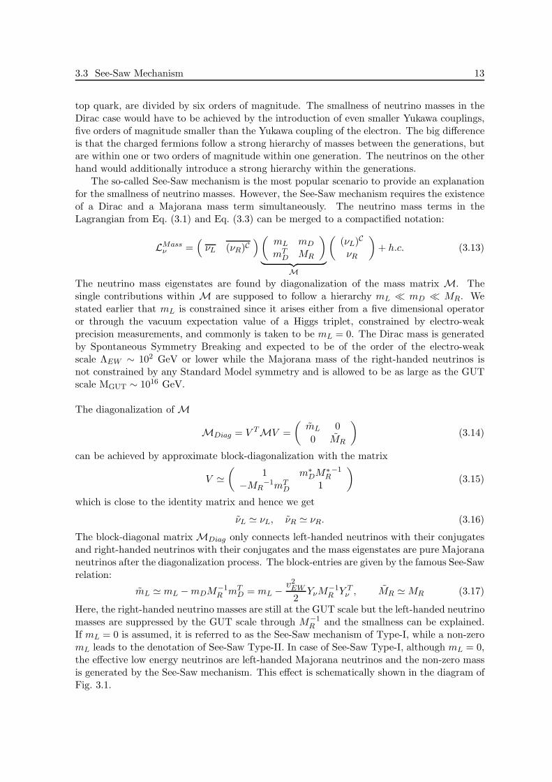
R and the smallness can be explained.If mL = 0 is assumed, it is referred to as the See-Saw mechanism of Type-I, while a non-zeromL leads to the denotation of See-Saw Type-II. In case of See-Saw Type-I, although mL = 0,the effective low energy neutrinos are left-handed Majorana neutrinos and the non-zero massis generated by the See-Saw mechanism. This effect is schematically shown in the diagram ofFig. 3.1.

14 CHAPTER 3. Neutrino Masses and Mixing

νL νLνR

φ0

νR

φ0

mD MRmD

vEW vEW

Figure 3.1: Diagramatic illustration of the generation of an effective left-handed majorana mass operatormL of light neutrinos through the See-Saw mechanism involving the Dirac mass term and the Majorana massterm of the heavy right-handed neutrinos νR.

3.4 Implications

The presence of neutrino masses and neutrino mixing implies additional phenomenologicalconsequences compared to the Standard Model. We will review in this section the threemost interesting possible implications of neutrino masses. Neutrino oscillations have alreadybeen established and confirm that neutrinos indeed do have a mass and there is mixingbetween the neutrino flavor eigenstates. For the oscillation mechanism to work, the natureof neutrino masses, i.e. if they are Majorana or Dirac particles, is not relevant and hencethis cannot be observed in neutrino oscillations. The further discussed possible implicationsof masses and mixing are the famous neutrino-less double beta decay, in abbreviation 0νββ,and Leptogenesis, i.e. the mechanism to explain the baryon asymmetry of our universe by thedecay of heavy right-handed neutrinos in the early universe.

Neutrino Oscillations

Here, we will only briefly discuss the framework of neutrino oscillations as they are implicationsof non-zero neutrino masses and neutrino mixing. Since neutrino oscillations are the topicof this work, a more detailed introduction to the framework is given in the next chapter.Neutrino oscillations can be understood in a complete quantum mechanical framework. Thefirst description of neutrino oscillations was given in [14] but for ν ↔ ν, whereas the firstdiscussion of neutrino oscillations between the flavor eigenstates was given in [15, 16]. Thestarting point is the neutrino mixing described by the unitary mixing matrix as introducedin Eq. (3.12):

|να〉 =∑

i

U∗αi|νi〉

The time evolution of the neutrino states is described by the Schrodinger equation, hereformulated for neutrino mass eigenstates in the rest frame of the neutrinos:

i∂

∂τi|νi〉 = H|νi〉 = mi|νi〉 (3.18)

Thus, the time evolution of the neutrino mass eigenstates is described by a time dependentcomplex phase factor:

|νi(τi)〉 = e−imiτi |νi(0)〉. (3.19)

However, the time evolution is required to be described in the laboratory frame where themeasurements take place. We will only consider relativistic neutrinos since the neutrino mass

3.4 Implications 15

is very small and all considered neutrino energies throughout this work will satisfy the con-dition Eν ≫ mν . The phase exponent in the time evolution of the neutrino mass eigenstatesin the laboratory system is expressed in terms of neutrino energy Ei and momentum pi as

miτi = Eit − pix = Eit −√

E2i − m2

i x

≃ Et − Ex +m2

i

2Ex

≃ m2i

2Ex =

m2i

2EL (3.20)

where we have used the expansion of the square root and the relativistic approximation x ≈ t.Furthermore, we have introduced the baseline L, i.e. the distance between the location ofneutrino production and detection. It can be seen that the phase factor can be approximatedand expressed in terms of squared neutrino masses2.

Now, the relevant aspect leading to neutrino oscillations is that neutrinos can only beproduced or detected in charged current weak interaction processes where only neutrino fla-vor eigenstates participate. Between production and detection the neutrinos propagate assuperposition of neutrino mass eigenstates with different evolutions of the phase factors andflavor transitions become possible, i.e. the detection of a neutrino of different flavor as theflavor of the initially produced neutrino. The probability Pαβ of such a flavor transition fromflavor α to flavor β is again calculated in the simple quantum mechanical picture:

|ν(t = 0)〉 = |να〉 =∑

k

U∗αk|νk〉 (3.21)

Pαβ = |〈νβ|ν(t)〉|2 =

∣∣∣∣∣

∑

k

U∗αke

−im2

k2E

L〈νβ |νk〉∣∣∣∣∣

2

=

∣∣∣∣∣∣

∑

k,j

UβjU∗αke

−im2

k2E

L〈νj |νk〉

∣∣∣∣∣∣

2

=

∣∣∣∣∣

∑

k

UβkU∗αke

−im2

k2E

L

∣∣∣∣∣

2

=∑

k,j

UβkU∗αkU

∗βjUαje

−im2

k−m2j

2EL (3.22)

It arises that the transition probability has indeed an oscillatory behavior since it is 2π-periodic in the parameter L/E, i.e. for a fixed neutrino energy the probability oscillates withthe distance from the location of neutrino production. Besides, it is obvious that a non-zerotransition probability between the different flavors α 6= β can only be obtained if neutrinomixing and non-zero neutrino masses are present simultaneously. If only one is present, i.e.either neutrino mixing of massless neutrinos or no mixing of massive neutrinos, no neutrinooscillations can occur:

2Note, that this is similar to the equal energy approximation (all mass eigenstates have equal energiesEi = E) which is in principle not the correct assumption but gives the right result as does the opposed equalmomenta approximation (all mass eigenstates have equal momenta pi = p). In general, the kinematics of theprocess where the neutrino is produced has to be taken accurately into account. See [17] or the review [18] fordetails of the discussion.

16 CHAPTER 3. Neutrino Masses and Mixing

Ν1

Ν2

Ν3

Ν1

Ν2

Ν3

Normal Hierarchy Inverted Hierarchy

Νe ΝΜ ΝΤ

Atm

ospheric

Solar

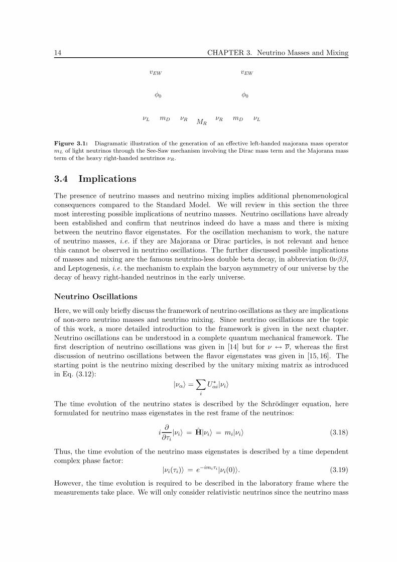
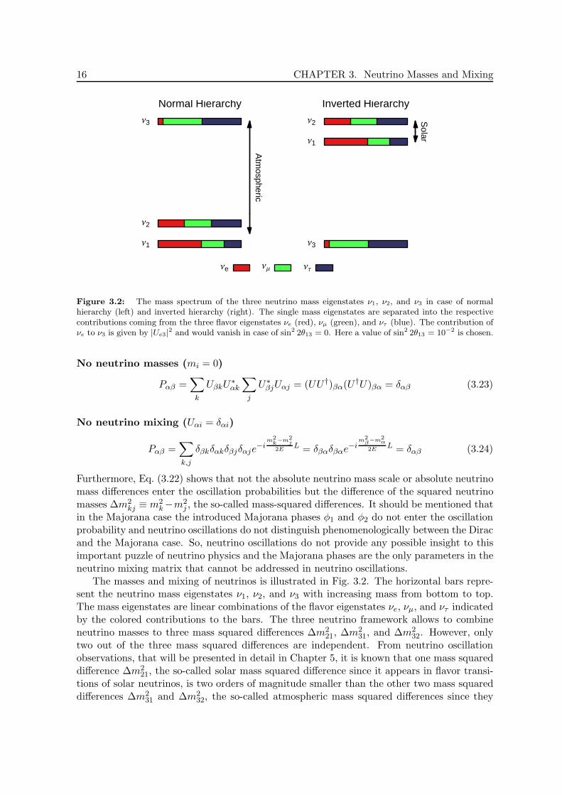
Figure 3.2: The mass spectrum of the three neutrino mass eigenstates ν1, ν2, and ν3 in case of normalhierarchy (left) and inverted hierarchy (right). The single mass eigenstates are separated into the respectivecontributions coming from the three flavor eigenstates νe (red), νµ (green), and ντ (blue). The contribution ofνe to ν3 is given by |Ue3|

2 and would vanish in case of sin2 2θ13 = 0. Here a value of sin2 2θ13 = 10−2 is chosen.

No neutrino masses (mi = 0)

Pαβ =∑

k

UβkU∗αk

∑

j

U∗βjUαj = (UU †)βα(U †U)βα = δαβ (3.23)

No neutrino mixing (Uαi = δαi)

Pαβ =∑

k,j

δβkδαkδβjδαje−i

m2k−m2

j2E

L = δβαδβαe−im2

β−m2α

2EL = δαβ (3.24)

Furthermore, Eq. (3.22) shows that not the absolute neutrino mass scale or absolute neutrinomass differences enter the oscillation probabilities but the difference of the squared neutrinomasses ∆m2

kj ≡ m2k−m2

j , the so-called mass-squared differences. It should be mentioned thatin the Majorana case the introduced Majorana phases φ1 and φ2 do not enter the oscillationprobability and neutrino oscillations do not distinguish phenomenologically between the Diracand the Majorana case. So, neutrino oscillations do not provide any possible insight to thisimportant puzzle of neutrino physics and the Majorana phases are the only parameters in theneutrino mixing matrix that cannot be addressed in neutrino oscillations.

The masses and mixing of neutrinos is illustrated in Fig. 3.2. The horizontal bars repre-sent the neutrino mass eigenstates ν1, ν2, and ν3 with increasing mass from bottom to top.The mass eigenstates are linear combinations of the flavor eigenstates νe, νµ, and ντ indicatedby the colored contributions to the bars. The three neutrino framework allows to combineneutrino masses to three mass squared differences ∆m2

21, ∆m231, and ∆m2

32. However, onlytwo out of the three mass squared differences are independent. From neutrino oscillationobservations, that will be presented in detail in Chapter 5, it is known that one mass squareddifference ∆m2

21, the so-called solar mass squared difference since it appears in flavor transi-tions of solar neutrinos, is two orders of magnitude smaller than the other two mass squareddifferences ∆m2

31 and ∆m232, the so-called atmospheric mass squared differences since they

3.4 Implications 17

du

W

e−

νe νe

W

e− u

dmee

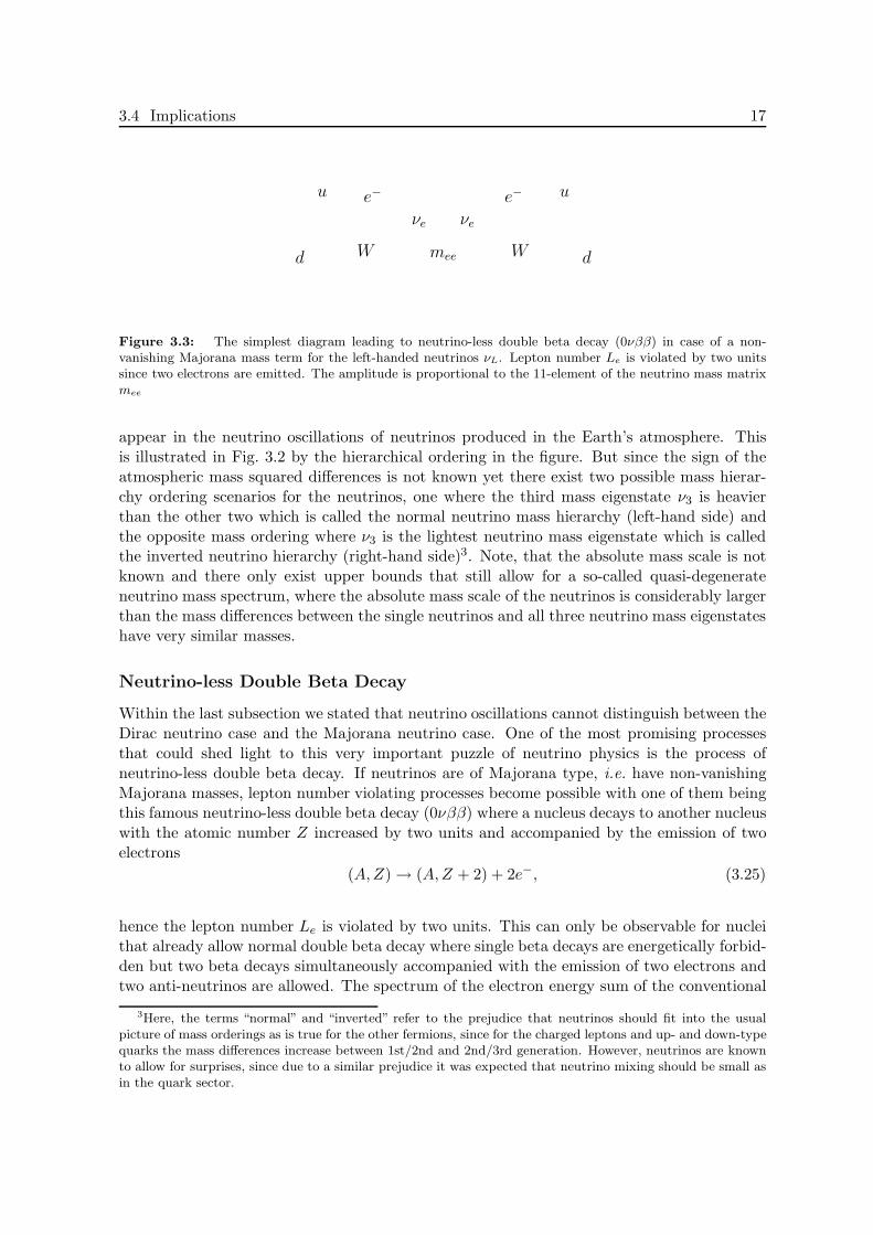
Figure 3.3: The simplest diagram leading to neutrino-less double beta decay (0νββ) in case of a non-vanishing Majorana mass term for the left-handed neutrinos νL. Lepton number Le is violated by two unitssince two electrons are emitted. The amplitude is proportional to the 11-element of the neutrino mass matrixmee

appear in the neutrino oscillations of neutrinos produced in the Earth’s atmosphere. Thisis illustrated in Fig. 3.2 by the hierarchical ordering in the figure. But since the sign of theatmospheric mass squared differences is not known yet there exist two possible mass hierar-chy ordering scenarios for the neutrinos, one where the third mass eigenstate ν3 is heavierthan the other two which is called the normal neutrino mass hierarchy (left-hand side) andthe opposite mass ordering where ν3 is the lightest neutrino mass eigenstate which is calledthe inverted neutrino hierarchy (right-hand side)3. Note, that the absolute mass scale is notknown and there only exist upper bounds that still allow for a so-called quasi-degenerateneutrino mass spectrum, where the absolute mass scale of the neutrinos is considerably largerthan the mass differences between the single neutrinos and all three neutrino mass eigenstateshave very similar masses.

Neutrino-less Double Beta Decay

Within the last subsection we stated that neutrino oscillations cannot distinguish between theDirac neutrino case and the Majorana neutrino case. One of the most promising processesthat could shed light to this very important puzzle of neutrino physics is the process ofneutrino-less double beta decay. If neutrinos are of Majorana type, i.e. have non-vanishingMajorana masses, lepton number violating processes become possible with one of them beingthis famous neutrino-less double beta decay (0νββ) where a nucleus decays to another nucleuswith the atomic number Z increased by two units and accompanied by the emission of twoelectrons

(A,Z) → (A,Z + 2) + 2e−, (3.25)

hence the lepton number Le is violated by two units. This can only be observable for nucleithat already allow normal double beta decay where single beta decays are energetically forbid-den but two beta decays simultaneously accompanied with the emission of two electrons andtwo anti-neutrinos are allowed. The spectrum of the electron energy sum of the conventional

3Here, the terms “normal” and “inverted” refer to the prejudice that neutrinos should fit into the usualpicture of mass orderings as is true for the other fermions, since for the charged leptons and up- and down-typequarks the mass differences increase between 1st/2nd and 2nd/3rd generation. However, neutrinos are knownto allow for surprises, since due to a similar prejudice it was expected that neutrino mixing should be small asin the quark sector.

18 CHAPTER 3. Neutrino Masses and Mixing

e−

u

e−

u

νe νe

Wd

Wd

0νββ

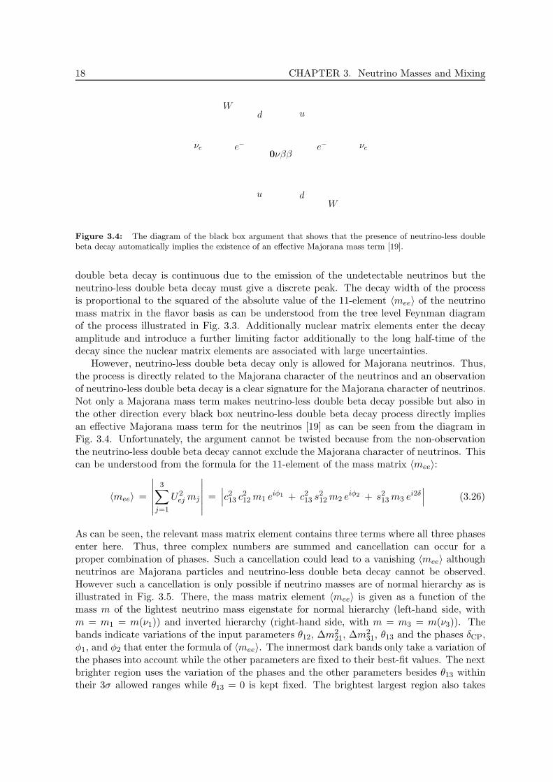
Figure 3.4: The diagram of the black box argument that shows that the presence of neutrino-less doublebeta decay automatically implies the existence of an effective Majorana mass term [19].

double beta decay is continuous due to the emission of the undetectable neutrinos but theneutrino-less double beta decay must give a discrete peak. The decay width of the processis proportional to the squared of the absolute value of the 11-element 〈mee〉 of the neutrinomass matrix in the flavor basis as can be understood from the tree level Feynman diagramof the process illustrated in Fig. 3.3. Additionally nuclear matrix elements enter the decayamplitude and introduce a further limiting factor additionally to the long half-time of thedecay since the nuclear matrix elements are associated with large uncertainties.

However, neutrino-less double beta decay only is allowed for Majorana neutrinos. Thus,the process is directly related to the Majorana character of the neutrinos and an observationof neutrino-less double beta decay is a clear signature for the Majorana character of neutrinos.Not only a Majorana mass term makes neutrino-less double beta decay possible but also inthe other direction every black box neutrino-less double beta decay process directly impliesan effective Majorana mass term for the neutrinos [19] as can be seen from the diagram inFig. 3.4. Unfortunately, the argument cannot be twisted because from the non-observationthe neutrino-less double beta decay cannot exclude the Majorana character of neutrinos. Thiscan be understood from the formula for the 11-element of the mass matrix 〈mee〉:

〈mee〉 =

∣∣∣∣∣∣

3∑

j=1

U2ej mj

∣∣∣∣∣∣

=∣∣∣c2

13 c212 m1 eiφ1 + c2

13 s212 m2 eiφ2 + s2

13 m3 ei2δ∣∣∣ (3.26)

As can be seen, the relevant mass matrix element contains three terms where all three phasesenter here. Thus, three complex numbers are summed and cancellation can occur for aproper combination of phases. Such a cancellation could lead to a vanishing 〈mee〉 althoughneutrinos are Majorana particles and neutrino-less double beta decay cannot be observed.However such a cancellation is only possible if neutrino masses are of normal hierarchy as isillustrated in Fig. 3.5. There, the mass matrix element 〈mee〉 is given as a function of themass m of the lightest neutrino mass eigenstate for normal hierarchy (left-hand side, withm = m1 = m(ν1)) and inverted hierarchy (right-hand side, with m = m3 = m(ν3)). Thebands indicate variations of the input parameters θ12, ∆m2

21, ∆m231, θ13 and the phases δCP,

φ1, and φ2 that enter the formula of 〈mee〉. The innermost dark bands only take a variation ofthe phases into account while the other parameters are fixed to their best-fit values. The nextbrighter region uses the variation of the phases and the other parameters besides θ13 withintheir 3σ allowed ranges while θ13 = 0 is kept fixed. The brightest largest region also takes

3.4 Implications 19

10-4 10-3 10-2 10-1 1

m @eVD

10-4

10-3

10-2

10-1

1

Xmee\@e

VD

Normal HierarchyDisfavored by 0ΝΒΒ Data

Disfavored

byC

osmologicalD

ata

10-4 10-3 10-2 10-1 1

m @eVD

10-4

10-3

10-2

10-1

1

Xmee\@e

VD

Normal Hierarchy

10-4 10-3 10-2 10-1 1

m @eVD

10-4

10-3

10-2

10-1

1

Xmee\@e

VD

Inverted HierarchyDisfavored by 0ΝΒΒ Data

Disfavored

byC

osmologicalD

ata

10-4 10-3 10-2 10-1 1

m @eVD

10-4

10-3

10-2

10-1

1

Xmee\@e

VD

Inverted Hierarchy

Figure 3.5: The possible values of the effective neutrino mass 〈mee〉 relevant in 0νββ decay as a functionof the lightest neutrino mass m for the normal mass hierarchy m = m1 < m2 < m3 (left) and the invertedmass hierarchy m = m3 < m1 < m2 (right). The inner (darkest) regions are obtained with the best-fit valuesof the oscillation parameters and only the CP phases φ1, φ1, and δ are kept free. The next brighter regionis obtained by the variation of the phases and the oscillation parameters θ12, ∆m2

21, and ∆m231 within the

allowed 3σ ranges while θ13 is fixed to be zero. The outmost brightest region is obtained by a variation of allrelevant parameters in 〈mee〉 within their allowed 3σ ranges.

into account a variation of θ13 within the allowed 3σ range. In case of normal hierarchy weobserve that for intermediate neutrino masses 10−2 eV < m < 10−3 eV indeed a cancellationof 〈mee〉 is possible while for inverted hierarchy this is never the case and 〈mee〉 & 10−2 eVholds independent of the magnitude of neutrino masses. Thus, neutrino-less double beta decaycould provide a possibility for the discrimination between normal and inverted hierarchy ofneutrinos.

Leptogenesis

Extensions of the Standard Model that include neutrino masses additionally offer a promisingexplanation for the baryon asymmetry of our universe. The amount of the observed presentbaryon asymmetry is generally described with the quantity

nb − nb

nγ= 6.15 ± 0.25 · 10−10 (3.27)

that relates the difference in the number density of baryons and anti-baryons to the presentnumber density of photons in the universe. This number is obtained from observations ofthe fluctuations in the Cosmic Microwave Background at WMAP [20] and shows that onlya tiny asymmetry, i.e. a tiny excess of matter over anti-matter, is required at the time thephotons decouple to explain the very large asymmetry we observe today. It was found thatany mechanism that can provide an explanation for the baryon asymmetry of the universemust fulfill the three Sakharov conditions [21] that are baryon number violation, C and CPviolation, and a deviation from thermal equilibrium. In principle these conditions can befulfilled in the Standard Model but it is still not able to explain the observed asymmetry.

20 CHAPTER 3. Neutrino Masses and Mixing

Ni

lα

φ

(Yν)αiNi

lα

φ

φ

lβ

Nj

(Yν)∗βi

(Yν)αj

(Yν)βj

Ni

lα

φ

Nj

lβ

φ

(Yν)αj

(Yν)∗βi (Yν)βj

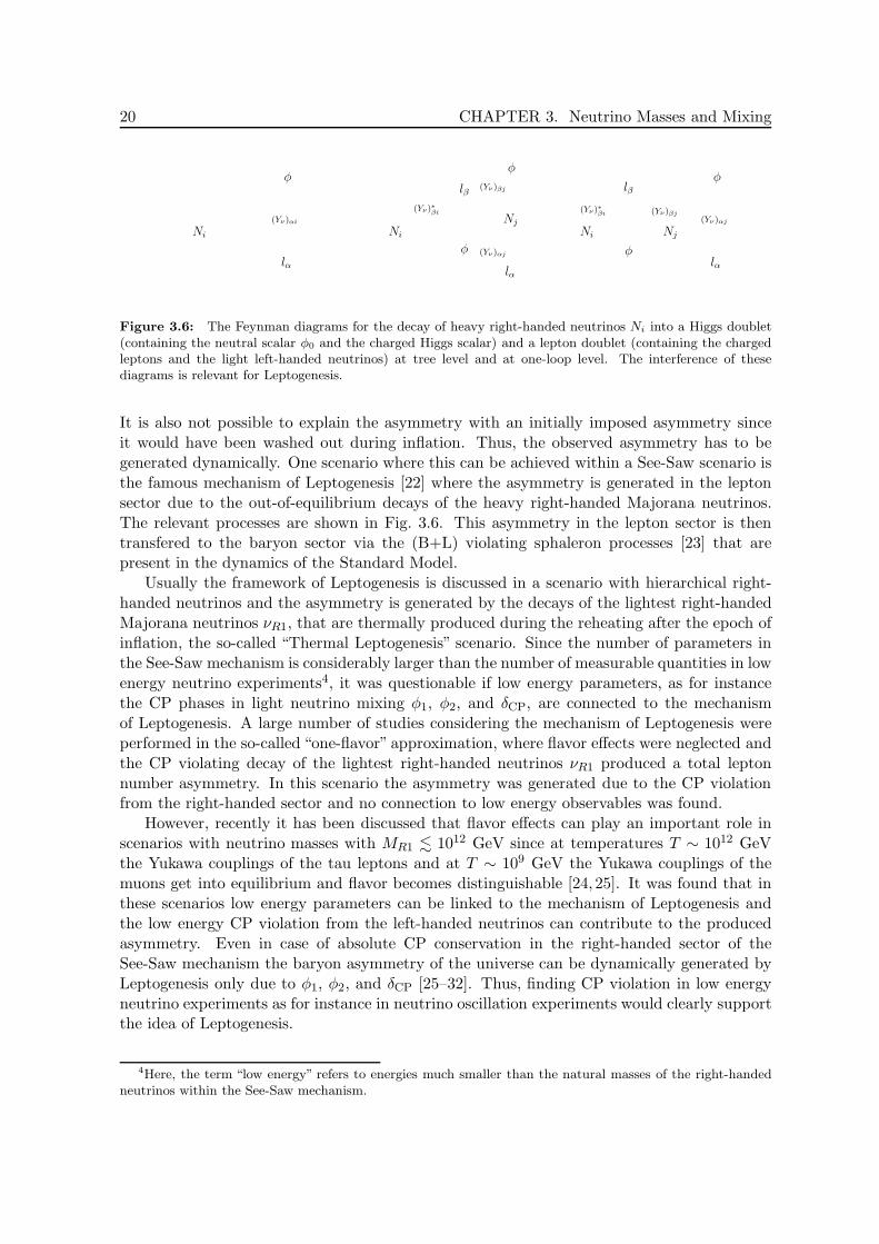
Figure 3.6: The Feynman diagrams for the decay of heavy right-handed neutrinos Ni into a Higgs doublet(containing the neutral scalar φ0 and the charged Higgs scalar) and a lepton doublet (containing the chargedleptons and the light left-handed neutrinos) at tree level and at one-loop level. The interference of thesediagrams is relevant for Leptogenesis.

It is also not possible to explain the asymmetry with an initially imposed asymmetry sinceit would have been washed out during inflation. Thus, the observed asymmetry has to begenerated dynamically. One scenario where this can be achieved within a See-Saw scenario isthe famous mechanism of Leptogenesis [22] where the asymmetry is generated in the leptonsector due to the out-of-equilibrium decays of the heavy right-handed Majorana neutrinos.The relevant processes are shown in Fig. 3.6. This asymmetry in the lepton sector is thentransfered to the baryon sector via the (B+L) violating sphaleron processes [23] that arepresent in the dynamics of the Standard Model.

Usually the framework of Leptogenesis is discussed in a scenario with hierarchical right-handed neutrinos and the asymmetry is generated by the decays of the lightest right-handedMajorana neutrinos νR1, that are thermally produced during the reheating after the epoch ofinflation, the so-called “Thermal Leptogenesis” scenario. Since the number of parameters inthe See-Saw mechanism is considerably larger than the number of measurable quantities in lowenergy neutrino experiments4, it was questionable if low energy parameters, as for instancethe CP phases in light neutrino mixing φ1, φ2, and δCP, are connected to the mechanismof Leptogenesis. A large number of studies considering the mechanism of Leptogenesis wereperformed in the so-called “one-flavor” approximation, where flavor effects were neglected andthe CP violating decay of the lightest right-handed neutrinos νR1 produced a total leptonnumber asymmetry. In this scenario the asymmetry was generated due to the CP violationfrom the right-handed sector and no connection to low energy observables was found.

However, recently it has been discussed that flavor effects can play an important role inscenarios with neutrino masses with MR1 . 1012 GeV since at temperatures T ∼ 1012 GeVthe Yukawa couplings of the tau leptons and at T ∼ 109 GeV the Yukawa couplings of themuons get into equilibrium and flavor becomes distinguishable [24, 25]. It was found that inthese scenarios low energy parameters can be linked to the mechanism of Leptogenesis andthe low energy CP violation from the left-handed neutrinos can contribute to the producedasymmetry. Even in case of absolute CP conservation in the right-handed sector of theSee-Saw mechanism the baryon asymmetry of the universe can be dynamically generated byLeptogenesis only due to φ1, φ2, and δCP [25–32]. Thus, finding CP violation in low energyneutrino experiments as for instance in neutrino oscillation experiments would clearly supportthe idea of Leptogenesis.

4Here, the term “low energy” refers to energies much smaller than the natural masses of the right-handedneutrinos within the See-Saw mechanism.

21

Chapter 4

Neutrino Oscillations

In the last chapter, we already introduced neutrino oscillations alongside the implicationsof neutrino masses and neutrino mixing. There it has been shown that both, masses andmixing, is required to allow the oscillatory flavor transitions between the neutrinos. In thischapter, we will review the phenomenology of neutrino oscillations in greater detail sincewe will focus on neutrino oscillation experiments in later chapters. First, we will address thesimple framework of two flavor oscillations because the framework is most comprehensible andfurther phenomenological consequences such as the matter effect can already be discussed in atwo flavor scenario. After that, we will switch to the three flavor framework and the additionalthree flavor effects compared to the two flavor framework will become apparent.

4.1 Two Flavor Oscillations

In the two flavor framework we will work in a two dimensional flavor space. i.e. there are twoflavor eigenstates |να〉 and |νβ〉 and two mass eigenstates |ν1〉 and |ν2〉. These states are againrelated by the neutrino mixing matrix, now called U :

|να〉 =

2∑

i=1

U∗αi |νi〉 (4.1)

This neutrino mixing matrix is now a unitary 2×2 matrix and in this case only one mixingangle is sufficient for the parameterization of the matrix:

(|να〉|νβ〉

)

=

(cos θ sin θ− sin θ cos θ

)(|ν1〉|ν2〉

)

(4.2)

We will now address the calculation of the disappearance probability for a neutrino that isproduced as a flavor eigenstate |να〉 and after propagation over the distance of the baseline L itis detected as a neutrino flavor eigenstate |νβ〉, i.e. a flavor transition has been occurred. Thepropagation is described by the Schrodinger equation with a Hamiltonian that is diagonalin the basis of mass eigenstates |ν1〉 and |ν2〉 and the propagation of mass eigenstates canbe described by a complex phase factor as given in Chapter 3.4, but the initial neutrino isproduced as a flavor eigenstate |ν(t = 0)〉 = |να〉. The oscillation probability is calculated by

22 CHAPTER 4. Neutrino Oscillations

Baseline L

Osc

illat

ion

Pro

babi

lity

PΑΑ

PΑΒ

sin2

2Θ

8 Π EΝ

Dm2

Baseline L

Osc

illat

ion

Pro

babi

lity

Energy EΝ

Osc

illat

ion

Pro

babi

lity

sin2

2Θ

Dm2 L

2 Π

PΑΑ

PΑΒ

Energy EΝ

Osc

illat

ion

Pro

babi

lity

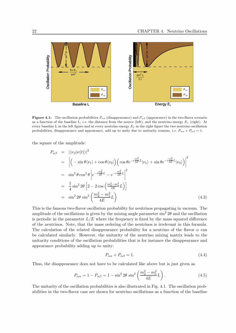
Figure 4.1: The oscillation probabilities Pαα (disappearance) and Pαβ (appearance) in the two-flavor scenarioas a function of the baseline L, i.e. the distance from the source (left), and the neutrino energy Eν (right). Atevery baseline L in the left figure and at every neutrino energy Eν in the right figure the two neutrino oscillationprobabilities, disappearance and appearance, add up to unity due to unitarity reasons, i.e. Pαα + Pαβ = 1.

the square of the amplitude:

Pαβ = |〈νβ|ν(t)〉|2

=

∣∣∣∣

(

− sin θ〈ν1| + cos θ〈ν2|)(

cos θe−im2

12E

L|ν1〉 + sin θe−im2

22E

L|ν2〉)∣∣∣∣

2

= sin2 θ cos2 θ

∣∣∣∣e−i

m22

2EL − e−i

m21

2EL

∣∣∣∣

2

=1

4sin2 2θ

[

2 − 2 cos(

m22−m2

1

2E L)]

= sin2 2θ sin2

(m2

2 − m21

4EL

)

(4.3)

This is the famous two-flavor oscillation probability for neutrinos propagating in vacuum. Theamplitude of the oscillations is given by the mixing angle parameter sin2 2θ and the oscillationis periodic in the parameter L/E where the frequency is fixed by the mass squared differenceof the neutrinos. Note, that the mass ordering of the neutrinos is irrelevant in this formula.The calculation of the related disappearance probability for a neutrino of the flavor α canbe calculated similarly. However, the unitarity of the neutrino mixing matrix leads to theunitarity conditions of the oscillation probabilities that is for instance the disappearance andappearance probability adding up to unity:

Pαα + Pαβ = 1. (4.4)

Thus, the disappearance does not have to be calculated like above but is just given as

Pαα = 1 − Pαβ = 1 − sin2 2θ sin2

(m2

2 − m21

4EL

)

. (4.5)

The unitarity of the oscillation probabilities is also illustrated in Fig. 4.1. The oscillation prob-abilities in the two-flavor case are shown for neutrino oscillations as a function of the baseline

4.2 Matter Effects 23

νe/νµ/ντ p/n/e−

νe/νµ/ντ

Z

p/n/e−

νe e−

e−

W

νe

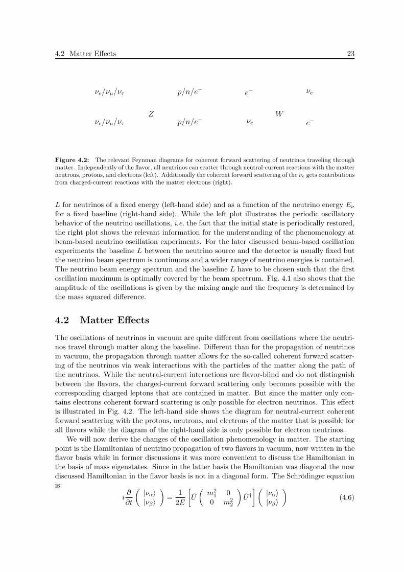
Figure 4.2: The relevant Feynman diagrams for coherent forward scattering of neutrinos traveling throughmatter. Independently of the flavor, all neutrinos can scatter through neutral-current reactions with the matterneutrons, protons, and electrons (left). Additionally the coherent forward scattering of the νe gets contributionsfrom charged-current reactions with the matter electrons (right).

L for neutrinos of a fixed energy (left-hand side) and as a function of the neutrino energy Eν

for a fixed baseline (right-hand side). While the left plot illustrates the periodic oscillatorybehavior of the neutrino oscillations, i.e. the fact that the initial state is periodically restored,the right plot shows the relevant information for the understanding of the phenomenology atbeam-based neutrino oscillation experiments. For the later discussed beam-based oscillationexperiments the baseline L between the neutrino source and the detector is usually fixed butthe neutrino beam spectrum is continuous and a wider range of neutrino energies is contained.The neutrino beam energy spectrum and the baseline L have to be chosen such that the firstoscillation maximum is optimally covered by the beam spectrum. Fig. 4.1 also shows that theamplitude of the oscillations is given by the mixing angle and the frequency is determined bythe mass squared difference.

4.2 Matter Effects

The oscillations of neutrinos in vacuum are quite different from oscillations where the neutri-nos travel through matter along the baseline. Different than for the propagation of neutrinosin vacuum, the propagation through matter allows for the so-called coherent forward scatter-ing of the neutrinos via weak interactions with the particles of the matter along the path ofthe neutrinos. While the neutral-current interactions are flavor-blind and do not distinguishbetween the flavors, the charged-current forward scattering only becomes possible with thecorresponding charged leptons that are contained in matter. But since the matter only con-tains electrons coherent forward scattering is only possible for electron neutrinos. This effectis illustrated in Fig. 4.2. The left-hand side shows the diagram for neutral-current coherentforward scattering with the protons, neutrons, and electrons of the matter that is possible forall flavors while the diagram of the right-hand side is only possible for electron neutrinos.

We will now derive the changes of the oscillation phenomenology in matter. The startingpoint is the Hamiltonian of neutrino propagation of two flavors in vacuum, now written in theflavor basis while in former discussions it was more convenient to discuss the Hamiltonian inthe basis of mass eigenstates. Since in the latter basis the Hamiltonian was diagonal the nowdiscussed Hamiltonian in the flavor basis is not in a diagonal form. The Schrodinger equationis:

i∂

∂t

(|να〉|νβ〉

)

=1

2E

[

U

(m2

1 00 m2

2

)

U †](

|να〉|νβ〉

)

(4.6)

24 CHAPTER 4. Neutrino Oscillations

and the Hamiltonian is a 2×2 matrix that also contains the mixing matrix:

HVAC =1

2E

[

U

(m2

1 00 m2

2

)

U †]

(4.7)

For the discussion of matter effects it is convenient to rewrite the Hamiltonian. Subtracting oradding contributions that are proportional to the identity matrix 12×2 do shift the eigenvaluesof the Hamiltonian but the dynamics of oscillations between the flavors are not affected by sucha transformation since this is only leading to an overall phase shift while neutrino oscillationsare the outcome of phase differences1. By making use of this effect the derivation of mattereffects becomes more convenient.

First, the Hamiltonian of vacuum oscillations is written explicitely in the flavor basis andsome trigonometric identities are used. Here, we already have subtracted a matrix propor-tional to the identity matrix to extract all dimensional quantities out of the matrix. Themodified Hamiltonian in Vacuum becomes:

HVAC =∆m2

21

2E

[

U

(0 00 1

)

U †]

=∆m2

21

4E

(1 − cos 2θ sin 2θ

sin 2θ 1 + cos 2θ

)

(4.8)

Furthermore, we can again safely subtract all contributions that are proportional to theidentity matrix and end up with the further modified Hamiltonian in vacuum in the flavorbasis of the two neutrino states:

HVAC =∆m2

21

4E

(− cos 2θ sin 2θsin 2θ + cos 2θ

)

(4.9)

Again, the eigenvalues have been shifted by the values that have been subtracted from thediagonal elements but the dynamics is still the same oscillation phenomenology that hasbeen derived in the last section. Now, if a propagation through matter is considered, thementioned coherent forward scattering adds contributions to the Hamiltonian that are theso-called effective matter potentials. We will here identify the flavor |να〉 with the electronneutrino and the flavor |νβ〉 with the muon neutrino or the tau neutrino. As could be readoff from Fig. 4.2, the neutrinos of flavor α can undergo neutral-current and charged-currentcoherent forward scattering while the neutrinos of flavor β are only sensitive to neutral-currentcoherent forward scattering. The relevant effective matter potential can be derived from theweak interaction part of the Lagrangian and are found to be:

ACC = ACC(t) =√

2GF NE(t), ANC = ANC(t) =1√2GF Nn(t) (4.10)

The effective matter potential for charged current scattering ACC is proportional to the elec-tron number density Ne and the effective coupling constant of the weak interactions, the Fermiconstant GF . The effective matter potentials for the neutral-current coherent forward scat-tering ANC is also proportional to the Fermi constant and additionally to the number densityof the neutrons2. These effective matter potential are now inserted to the Hamiltonian in

1Note, that this argument is independent of the basis and the subtractions can be performed in the flavorbasis and in the mass eigenstate basis.

2The scattering involves the protons, neutrons, and electrons of the matter but the contributions of protonsand electrons cancel out [33].

4.2 Matter Effects 25

the flavor basis on the respective diagonal elements since no flavor transitions are governeddirectly by the forward scattering and one ends up with the Hamiltonian in matter:

HMAT =∆m2

21

4E

(− cos 2θ sin 2θsin 2θ + cos 2θ

)

+

(ACC + ANC 0

0 ANC

)

(4.11)

Again, the contributions proportional to the identity matrix can be split off

HMAT =∆m2

21

4E

(−(cos 2θ − A′) sin 2θ

sin 2θ cos 2θ − A′

)

+

( ACC2 + ANC 0

0 ACC2 + ANC

)

(4.12)

and only the first term is relevant for the dynamics of neutrino oscillations. The only remainingcontribution from the matter through coherent forward scattering is coming from charged-current interactions of the neutrinos of flavor α. The effective matter potential ACC is hiddenin the dimensionless variable A′:

A′ ≡ 2E

∆m221

ACC (4.13)

Now, the new eigenvalues of the Hamiltonian in matter can be easily calculated:

λ1/2 = ∓∆m221

4E

√

sin2 2θ + (cos 2θ − A′)2 (4.14)

With an educated guess and this eigenvalues in mind one can rewrite the Hamiltonian inmatter as

HMAT =∆m2

21

√

sin2 2θ + (cos 2θ − A′)2

4E

− (cos 2θ−A′)√sin2 2θ+(cos 2θ−A′)2

sin 2θ√sin2 2θ+(cos 2θ−A′)2

sin 2θ√sin2 2θ+(cos 2θ−A′)2

cos 2θ−A′√sin2 2θ+(cos 2θ−A′)2

=∆m2

M

4E

(− cos 2θM sin 2θM

sin 2θM + cos 2θM

)

(4.15)

which after introducing the new parameters ∆m2M, sin 2θM, and cos 2θM takes again the form

of the vacuum Hamiltonian of Eq. (4.9). Thus the derived Hamiltonian in matter shows thesame phenomenology of neutrino oscillations as the Hamiltonian in vacuum but the vacuumparameters are modified by the matter potential parameter A′:

∆m2M = ∆m2

21

√

sin2 2θ + (cos 2θ − A′)2

sin 2θM =sin 2θ

√

sin2 2θ + (cos 2θ − A′)2

cos 2θM =cos 2θ − A′

√

sin2 2θ + (cos 2θ − A′)2(4.16)

In the case of anti-neutrinos traveling through the matter the sign of the effective matter po-tential has to be reversed and the oscillation parameters for anti-neutrinos in matter become:

∆m2M = ∆m2

21

√

sin2 2θ + (cos 2θ + A′)2

sin 2θM =sin 2θ

√

sin2 2θ + (cos 2θ + A′)2

cos 2θM =cos 2θ + A′

√

sin2 2θ + (cos 2θ + A′)2(4.17)

26 CHAPTER 4. Neutrino Oscillations

Constant Matter Density Profile

If the neutrinos travel through matter with constant matter density along the baseline, i.e.the effective matter potential parameter A′ stays constant and the oscillation parameters stayconstant along the baseline the new neutrino oscillation probabilities can be easily determined.Since the Hamiltonian is of the same form as the Hamiltonian in vacuum, the formulas forthe oscillation probabilities stay the same as derived in the vacuum case. However, theoscillation frequency and the oscillation amplitude are modified due to the presence of thematter potential. Without further calculation we can use the formulas from the last sectionand find for the oscillation probabilities for neutrinos traveling along a baseline of constantmatter density profile:

Pαα = 1 − sin2 2θM sin2

(∆m2

M

4EL

)

Pαβ = sin2 2θM sin2

(∆m2

M

4EL

)

Pαα = 1 − sin2 2θM sin2

(∆m2

M

4EL

)

Pαβ = sin2 2θM sin2

(∆m2

M

4EL

)

(4.18)

We find that different than in vacuum two-flavor oscillations the probabilities for neutrinosand anti-neutrinos differ since the effect of the matter potential is reversed for neutrinos andanti-neutrinos. Thus, a form of CP violation is introduced with the matter along the baseline.This has to be carefully distinguished from intrinsic CP violation that is introduced on anelementary basis since here the CP violation, i.e. different probabilities for neutrinos and anti-neutrinos is a consequence of the composition of the matter that is only containing matter andno anti-matter. This externally introduced CP violation is sometimes referred to as extrinsicCP violation. Intrinsic CP violation is, as we will see in the case of three-flavor oscillations,a possible consequence of a complex mixing matrix however in the two-flavor scenario themixing matrix is always real.

Mikheyev-Smirnov-Wolfenstein Resonance

A further important consequence of the matter potential is the so-called Mikheyev-Smirnov-Wolfenstein resonance. The oscillation parameters in matter differ from the original oscilla-tion parameters in vacuum as described in Eq. (4.16) for neutrinos and Eq. (4.17) for anti-neutrinos. There can occur a resonant enhancement of the mixing angle in matter dependingon the value of the dimensionless matter potential parameter A′. For special choices of A′

maximal mixing, i.e. a mixing angle of sin2 2θM = 1, can occur even for very small mixing invacuum, i.e. a small vacuum mixing angle sin2 2θ. The conditions are

cos 2θ − A′ = 0 → sin2 2θM = 1 (4.19)

for neutrinos and

cos 2θ + A′ = 0 → sin2 2θM = 1 (4.20)

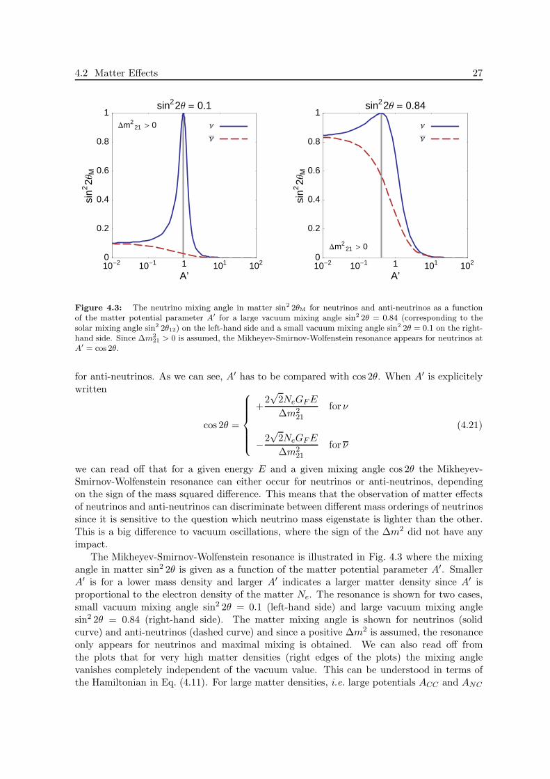
4.2 Matter Effects 27

10-2 10-1 1 101 102

A’

0

0.2

0.4

0.6

0.8

1

sin2

2ΘM

sin22Θ = 0.1

Dm221 > 0 Ν

Ν

10-2 10-1 1 101 102

A’

0

0.2

0.4

0.6

0.8

1

sin2

2ΘM

sin22Θ = 0.84

Dm221 > 0

Ν

Ν

Figure 4.3: The neutrino mixing angle in matter sin2 2θM for neutrinos and anti-neutrinos as a functionof the matter potential parameter A′ for a large vacuum mixing angle sin2 2θ = 0.84 (corresponding to thesolar mixing angle sin2 2θ12) on the left-hand side and a small vacuum mixing angle sin2 2θ = 0.1 on the right-hand side. Since ∆m2

21 > 0 is assumed, the Mikheyev-Smirnov-Wolfenstein resonance appears for neutrinos atA′ = cos 2θ.

for anti-neutrinos. As we can see, A′ has to be compared with cos 2θ. When A′ is explicitelywritten

cos 2θ =

+2√

2NeGF E

∆m221

for ν

−2√

2NeGF E

∆m221

for ν

(4.21)

we can read off that for a given energy E and a given mixing angle cos 2θ the Mikheyev-Smirnov-Wolfenstein resonance can either occur for neutrinos or anti-neutrinos, dependingon the sign of the mass squared difference. This means that the observation of matter effectsof neutrinos and anti-neutrinos can discriminate between different mass orderings of neutrinossince it is sensitive to the question which neutrino mass eigenstate is lighter than the other.This is a big difference to vacuum oscillations, where the sign of the ∆m2 did not have anyimpact.

The Mikheyev-Smirnov-Wolfenstein resonance is illustrated in Fig. 4.3 where the mixingangle in matter sin2 2θ is given as a function of the matter potential parameter A′. SmallerA′ is for a lower mass density and larger A′ indicates a larger matter density since A′ isproportional to the electron density of the matter Ne. The resonance is shown for two cases,small vacuum mixing angle sin2 2θ = 0.1 (left-hand side) and large vacuum mixing anglesin2 2θ = 0.84 (right-hand side). The matter mixing angle is shown for neutrinos (solidcurve) and anti-neutrinos (dashed curve) and since a positive ∆m2 is assumed, the resonanceonly appears for neutrinos and maximal mixing is obtained. We can also read off fromthe plots that for very high matter densities (right edges of the plots) the mixing anglevanishes completely independent of the vacuum value. This can be understood in terms ofthe Hamiltonian in Eq. (4.11). For large matter densities, i.e. large potentials ACC and ANC

28 CHAPTER 4. Neutrino Oscillations

the first part of the Hamiltonian can be neglected and only the second matrix forms theHamiltonian but this matrix is diagonal in the flavor-basis. Thus, the basis that provides adiagonal Hamiltonian, i.e. the basis of mass eigenstates, is already given in the flavor basis.So, for very high matter densities flavor and mass eigenstates are identical and no mixingoccurs. This effect is of importance for the understanding of the solar neutrino puzzle sincesolar neutrinos are produced in the interior of the sun at very high densities of ρ ∼ 150 g/cm3.This will be described in the next chapter in the context of the phenomenology of an adiabaticmatter density profile.

Adiabatic Matter Density Profile

Up to now we have only discussed neutrino propagation through constant matter denitiy pro-files. However some scenarios like the propagation of solar neutrinos cannot be approximatedwith a constant matter density profile. Solar neutrinos are produced in the middle of the sunat very high matter densities ρ ∼ 150 g/cm3 and then propagate outwards until they leave thesun. From the middle of the sun to the outer regions the matter density decreases continouslyuntil zero matter density, i.e. vacuum is reached. This can be approximated by the so-calledadiabatic matter density profile, where the matter density ρ, and thus also the matter densityparameter A′, changes adiabatically. Adiabatically here means that the change of matterdensity is very slow and the system can adjust adequately during the propagation. For aneutrino that is produced as a mass eigenstate at very high densities above the resonance thisimplies that the neutrino remains the same mass eigenstate during propagation through theadiabatically decreasing matter density and transitions between the mass eigenstates is sup-pressed. The eigenvalues of the Hamiltonian changes as a function of the matter density, i.e.the matter density parameter A′. The eigenvalues are

E1/2 =∆m2

21

4E

[

A′ ∓√

sin2 2θ + (cos 2θ − A′)2]

(4.22)

and the evolution as a function of A′ is given in the left-hand side of Fig. 4.4. Note, that theseeigenvalues are not the eigenvalues λ1/2 of the first term in the Hamiltonian in Eq. (4.12) butshifted with ACC/2 that is the diagonal part of the charged current matter potential that wasneglected for the calculation of λ1/2. But since we here are interested in the eigenvalues thispart is not neglected and E1/2 describe the full effect of the charged current coherent forwardscattering. The dashed lines in Fig. 4.4 appear for a vanishing mixing angle sin2 2θ = 0 andcross at the resonance, but if even a small mixing is introduced the curves avoid crossing.However, if the neutrino is produced at higher densities as a mass eigenstate and remainsthat state during the propagation through the adiabatically decreasing matter density, theflavor composition of this mass eigenstate changes due to the matter effect and an adiabaticconversion of flavors happens. This effect has to be distinguished from neutrino oscillations.The flavor conversion is illustrated in the right-hand side of Fig. 4.4. At the right edge theneutrino is produced as a να identical with the mass eigenstate ν2 at high matter densities.The neutrino state ν2 propagates to smaller matter densities and passes the resonance condi-tion (maximal mixing thus |〈ν2|να〉|2 = |〈ν2|νβ〉|2=0.5). For even smaller matter densities thecontribution of the flavor νβ even increases. Since the flavor composition of να in the propa-gating mass eigenstate ν2 in vacuum is given by the vacuum mixing |〈ν2|να〉|2 = sin2 θ for verysmall mixing angles the mass eigenstate ν2 can even be completely conversed adiabaticallyfrom flavor να to flavor νβ.

4.3 Three Flavor Oscillations 29

10-2 10-1 1 101 102

A’

Effe

ctiv

een

ergy

eige

nval

ues

E2

E1

10-2 10-1 1 101 102

A’

0

0.2

0.4

0.6

0.8

1

Mas

sei

gens

tate

com

posi

tion

ofΝ

Α

È<Ν2 ÈΝΒ >È2

È<Ν2 ÈΝΑ >È2

10-2 10-1 1 101 102

A’

0

0.2

0.4

0.6

0.8

1

Mas

sei

gens

tate

com

posi

tion

ofΝ

ΑFigure 4.4: The effective energy eigenvalues E1/2 in matter (left, logarithmic scaling) and the mass eigenstatecompositions |〈ν2|νβ〉|

2 = cos2 θM and |〈ν2|να〉|2 = sin2 θM of the flavor eigenstate |να〉 (right) as functions of

the matter potential parameter A′. The dashed lines in the left-hand side plot illustrate the behavior of theenergy eigenvalues in the case of no mixing. The horizontal grey dashed line corresponds to the value of thelarger vacuum energy eigenvalue E2(A

′ ≪ 0) = ∆m221/2E whereas the diagonal grey dashed line corresponds

to the larger energy eigenvalue in the limit of very high matter densities E2(A′ ≫ 0) = ∆m2

21A′/2E.

4.3 Three Flavor Oscillations

The framework of neutrino oscillations with three flavors is slightly more complicated com-pared to the two-flavor framework. The unitary mixing matrix contains four instead of onlyone parameter, that is three mixing angles θ12, θ13, θ23, and the phase δCP. The parame-terization of the mixing matrix was given in Chapter 3.23. However the basic principles arethe same. We begin with calculating the oscillation probabilities, now in the three-flavorframework.

Oscillation Probabilities

The starting point is Eq. (3.22) from the last chapter where an expression for the oscillationprobability was found independent of the number of flavors. Here, we assume a summationover the three indices of the three-dimensional flavor space (Latin indices sum over 1,2,3 andindicate mass eigenstates, Greek indices sum over the three flavors of the flavor eigenstatese, µ, τ).

Pαβ =∑

k,l

UβkU∗αkU

∗βlUαle

−im2

k−m2l

2EL

=∑

k

UβkU∗αkU

∗βkUαk + 2

∑

k>l

Re

[

UβkU∗αkU

∗βlUαl e

−im2

k−m2l

2EL

]

3We will now neglect the Majorana phases φ1 and φ2 because neutrino oscillations are not sensitive to theseparameters and the Majorana neutrino case cannot be distinguished from the Dirac neutrino case.

30 CHAPTER 4. Neutrino Oscillations

= δαβ −∑

i,j

UβiU∗αiU

∗βjUαj +

∑

k

UβkU∗αkU

∗βkUαk

+2∑

k>l

[

Re[UβkU

∗αkU

∗βlUαl

]cos(2∆kl) − Im

[UβkU

∗αkU

∗βlUαl

]sin(2∆kl)

]

= δαβ − 4∑

k>l

Re[UβkU

∗αkU

∗βlUαl

]sin2(∆kl)

−2∑

k>l

Im[UβkU

∗αkU

∗βlUαl

]sin(2∆kl) (4.23)

This is the famous general formula of neutrino oscillations. We have used the abbreviation∆2

kl ≡ ∆m2klL/2E. This expression holds for neutrinos and if anti-neutrinos are considered

the conjugated elements of the mixing matrix have to be taken. This transformation doesnot affect the first two terms of the expression however the third term switches the sign.So, if three-flavor oscillations are considered, a complex mixing matrix introduces differencesin the oscillation probabilities for neutrinos and anti-neutrinos, hence CP violation becomespossible. Since a complex phase was absent in the two-flavor scenario, CP violation could notarise for two flavors and intrinsic CP violation is a genuine effect for oscillations with morethan two flavors.

CP Violation

Intrinsic CP violation in vacuum oscillations arises not until three flavors are consideredand thus is called a genuine tree-flavor effect. Note that in the discussion of the mattereffect in the two-flavor scenario a difference in the oscillation probabilities of neutrinos andanti-neutrinos was obtained but this effect was due to the CP asymmetric composition ofthe matter along the baseline that is only containing matter and no anti-matter. This CPviolation is called extrinsic CP violation while the genuine CP violation that can arise evenfor vacuum oscillations in the three-flavor framework is referred to as intrinsic. CP violationin three-flavor vacuum oscillations is given in the case of differing oscillation probabilities:

P (να → νβ) 6= P (να → νβ). (4.24)

In Eq. (4.23) the CP violation arises due to the third term with the imaginary part of theproduct of neutrino mixing matrix entries. So, CP violation can only arise if the phase δCP

is not realized at one of the CP conserving values, i.e.:

δCP 6= 0, and δCP 6= π. (4.25)

If δCP deviates from these values the mixing matrix becomes complex and neutrino and anti-neutrino oscillation probabilities deviate. It can be derived that all CP violating quantitiescan be expressed with a parameter JCP that is similar to the Jarlskog parameter in the quarksector [34–36]. JCP is given as

JCP =1

8sin δCP cos θ13 sin 2θ12 sin 2θ13 sin 2θ23 (4.26)

In the parameterization of the mixing matrix the CP phase δCP is closely connected to themixing angle sin θ13 and in case of sin θ13 = 0 the parameter δCP is unphysical and CP violationis not possible. While this might appear to be a artificial preference of sin θ13 over the other

4.4 Phenomenology of Peµ and Pee 31

mixing parameters, the parameter JCP shows that this is not the case since every CP violatingquantity is proportional to JCP and thus vanishes for either of the three mixing angles equalto zero. So, three non-vanishing mixing angles are the requirement for CP violation to bepossible.

Furthermore, CP violation can only be observed in appearance channels. The disappear-ance channels cannot show CP violating effects because of the CPT theorem:

PααCP→ Pαα

T→ Pαα (4.27)

So, the relevant oscillation channels at future neutrino oscillation experiments for the searchof CP violation will be the appearance channels like for instance the golden channel at aNeutrino Factory, the oscillation channel νe → νµ.

Matter Effects in Three Flavors

Matter effects occur in the three flavor framework as well. The electron neutrinos can undergocharged current and neutral current coherent forward scattering while the other flavors νµ andντ only can scatter via neutral currents. As already in the two-flavor framework, the mattereffect can be described by adding an additional effective matter potential to the ee-elementin the Hamiltonian in the flavor basis. This corresponds to the framework with two flavors.The non-diagonal Hamiltonian is given as:

i∂

∂t

|νe〉|νµ〉|ντ 〉

=∆m2

31

2E

U

0 0 00 α 00 0 1

U † +

A 0 00 0 00 0 0

|νe〉|νµ〉|ντ 〉

. (4.28)

As in the two-flavor scenario the contributions from the neutral current coherent forwardscattering has been neglected since terms proportional to the identity matrix 13×3 do notcontribute to the oscillation phenomenology but only shift the eigenvalues. Additionally, alldimensional parameters have been extracted from the matrix by introducing the parameters

A ≡ 2E

∆m231

ACC , and α ≡ ∆m221

∆m231

. (4.29)

The oscillation parameters in matter can now be obtained by a re-diagonalization of the newHamiltonian and the original form of the vacuum Hamiltonian can be restored by switchingto new parameters, the mixing parameters in matter ∆m2

21,M, ∆m231,M, sin θ12,M, sin θ13,M,

sin θ23,M, and δCP,M. Different to the two-flavor framework not only one Mikheyev-Smirnov-Wolfenstein resonance is present since two frequencies ∆m2

21 and ∆m231 are introduced. The

explicit full formulas of the neutrino oscillation probabilities in matter have been derived andcan be found in [37,38]

4.4 Phenomenology of Peµ and Pee

The explicit full expressions for the neutrino oscillation probabilities in the three-flavor frame-work are quite extended and do not provide enough analytical insight to understand therelevant phenomenology. Thus, if one wants to understand the phenomenology of the perfor-mance of future and present beam based neutrino long baseline experiments, it has turned

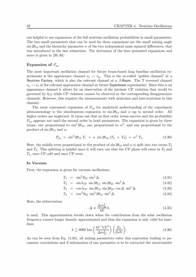
32 CHAPTER 4. Neutrino Oscillations

out helpful to use expansions of the full neutrino oscillation probabilities in small parameters.The two small parameters that can be used for these expansions are the small mixing anglesin 2θ13 and the hierarchy parameter α of the two independent mass squared differences, thatwas introduced in the last subsection. The derivation of the here presented expansions andmore is given in [39,40].

Expansion of Peµ

The most important oscillation channel for future beam-based long baseline oscillation ex-periments is the appearance channel νe → νµ. This is the so-called “golden channel” at aNeutrino Factory, which is also the relevant channel at a β-Beam. The T reversed channelνµ → νe is the relevant appearance channel at future Superbeam experiments. Since this is anappearance channel it allows for an observation of the intrinsic CP violation that would begoverned by δCP while CP violation cannot be observed at the corresponding disappearancechannels. However, this requires the measurements with neutrinos and anti-neutrinos in thischannel.

The most convenient expansion of Peµ for analytical understanding of the experimentphenomenology is the simultaneous expansion in sin 2θ13 and α up to second order. Allhigher orders are neglected. It turns out that no first order terms survive and the probabilityPeµ appears not until the second order in both parameters. The expansion is given by threeterms, one proportional to sin2 2θ13, one proportional to α2, and one proportional to theproduct of sin 2θ13 and α:

Peµ ≃ sin2 2θ13 T1 + α sin 2θ13 (T2 + T3) + α2 T4. (4.30)

Here, the middle term proportional to the product of sin 2θ13 and α is split into two terms T2

and T3. This splitting is helpful since it will turn out that the CP phase will enter in T2 andT3, once CP odd and once CP even.

In Vacuum

First, the expression is given for vacuum oscillations:

T1 = sin2 θ23 sin2 ∆ (4.31)

T2 = sin δCP sin 2θ12 sin 2θ23 sin3 ∆ (4.32)

T3 = cos δCP sin 2θ12 sin 2θ23 cos ∆ sin2 ∆ (4.33)

T4 = cos2 θ23 sin2 2θ12 sin2 ∆ (4.34)

Here, the abbreviation

∆ ≡ ∆m231

4EL (4.35)

is used. This approximation breaks down when the contribution from the solar oscillationfrequency cannot longer linearly approximated and thus the expansion is only valid for base-lines

L . 8000 km

(10−4eV2

∆m221

)(Eν

GeV

)

. (4.36)

As can be seen from Eq. (4.34), all mixing parameters enter this expression leading to pa-rameter correlations and if information of one parameter is to be extracted the uncertainties

4.4 Phenomenology of Peµ and Pee 33

on all other parameters come into play. For large sin2 2θ13 the first term containing T1 is thedominating term. For intermediate sin2 2θ13 however all four terms contribute with similarmagnitudes. Only for small or vanishing sin2 2θ13 the last term T4 dominates. It is apparentthat even for vanishing sin2 2θ13 the oscillation probability Peµ does not vanish because ofT4 6= 0.

However, the parameter correlations are not the only limiting factor if information onsingle parameters is to be extracted from oscillation data of this channel. It was observedthat the oscillation probability Peµ is invariant under a certain set of three independenttransformations leading to the so-called “eight-fold degeneracy” [41]. This set of degeneraciesis given by the following transformations:

• Intrinsic (θ13,δCP) degeneracy with (θ13,δCP) → (θ′13,δ′CP) [42]

• Sign-degeneracy with ∆m231 → −∆m2

31 [43]

• Octant-degeneracy with θ23 → π/2 − θ23 [44]

All of these parameter transformation and all combinations of these parameter transforma-tions lead to a degenerate solution in parameter space. In total there are eight combina-tions of parameter transformations thus the name of the eight-fold degeneracy. The intrinsic(θ13,δCP)-degeneracy is of continuous character. Given a true set of parameters with a truevalue of δCP the identical value for the oscillation probability can be obtained by any valuefor δCP by adjusting the value of sin 2θ13 appropriately. The sign-degeneracy appears forthe opposite sign of the atmospheric mass squared difference ∆m2

31, i.e. ∆ → −∆. Note,that only the sign of the second term T2 is changed by this transformation and this can beexactly compensated by a simultaneous sign change of the phase δCP → −δCP. The octantdegeneracy is given by the transformation of the atmospheric mixing angle θ23 → π/2 − θ23.This transformation corresponds to sin 2θ23 → sin 2θ23 and cos 2θ23 → − cos 2θ23 thus leavingthe oscillation probability Peµ invariant.

In Matter

The expression of the oscillation probability Peµ in matter has the similar structure than theexpression in vacuum but now the dimensionless parameter A that describes the effectivematter potential because of the coherent forward scattering is additionally introduced:

T1 = sin2 θ23sin2[(1 − A)∆]

(1 − A)2(4.37)

T2 = sin δCP sin 2θ12 sin 2θ23 sin∆sin(A∆)

A

sin[(1 − A)∆]

(1 − A)(4.38)

T3 = cos δCP sin 2θ12 sin 2θ23 cos ∆sin(A∆)

A

sin[(1 − A)∆]

(1 − A)(4.39)

T4 = cos2 θ23 sin2 2θ12sin2(A∆)

A2(4.40)

The validity of this expansion depends on the baseline and is given as in Eq. (4.36) butsince the solar resonance is not covered by the expansion further restrictions for the neutrino

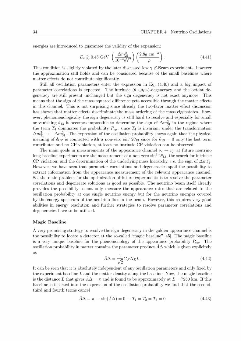
34 CHAPTER 4. Neutrino Oscillations

energies are introduced to guarantee the validity of the expansion:

Eν & 0.45 GeV

(∆m2

21

10−4eV2

)(2.8g cm−3

ρ

)

. (4.41)

This condition is slightly violated by the later discussed low γ β-Beam experiments, howeverthe approximation still holds and can be considered because of the small baselines wherematter effects do not contribute significantly.

Still all oscillation parameters enter the expression in Eq. (4.40) and a big impact ofparameter correlations is expected. The intrinsic (θ13,δCP)-degeneracy and the octant de-generacy are still present unchanged but the sign degeneracy is not exact anymore. Thismeans that the sign of the mass squared difference gets accessible through the matter effectsin this channel. This is not surprising since already the two-favor matter effect discussionhas shown that matter effects discriminate the mass ordering of the mass eigenstates. How-ever, phenomenologically the sign degeneracy is still hard to resolve and especially for smallor vanishing θ13 it becomes impossible to determine the sign of ∆m2

31 in the regime wherethe term T4 dominates the probability Peµ, since T4 is invariant under the transformation∆m2

31 → −∆m231. The expression of the oscillation probability shows again that the physical

meaning of δCP is connected with a non-zero sin2 2θ13 since for θ13 = 0 only the last termcontributes and no CP violation, at least no intrinsic CP violation can be observed.

The main goals in measurements of the appearance channel νe → νµ at future neutrinolong baseline experiments are the measurement of a non-zero sin2 2θ13, the search for intrinsicCP violation, and the determination of the underlying mass hierarchy, i.e. the sign of ∆m2

31.However, we have seen that parameter correlations and degeneracies spoil the possibility toextract information from the appearance measurement of the relevant appearance channel.So, the main problem for the optimization of future experiments is to resolve the parametercorrelations and degenerate solutions as good as possible. The neutrino beam itself alreadyprovides the possibility to not only measure the appearance rates that are related to theoscillation probability at one single neutrino energy but for the neutrino energies coveredby the energy spectrum of the neutrino flux in the beam. However, this requires very goodabilities in energy resolution and further strategies to resolve parameter correlations anddegeneracies have to be utilized.

Magic Baseline

A very promising strategy to resolve the sign-degeneracy in the golden appearance channel isthe possibility to locate a detector at the so-called “magic baseline” [45]. The magic baselineis a very unique baseline for the phenomenology of the appearance probability Peµ. Theoscillation probability in matter contains the parameter product A∆ which is given explicitelyas

A∆ =1√2GF NEL. (4.42)

It can be seen that it is absolutely independent of any oscillation parameters and only fixed bythe experiment baseline L and the matter density along the baseline. Now, the magic baselineis the distance L that gives A∆ = π and is found to be approximately at L = 7250 km. If thisbaseline is inserted into the expression of the oscillation probability we find that the second,third and fourth terms cancel

A∆ ≡ π → sin(A∆) = 0 → T1 = T2 = T3 = 0 (4.43)

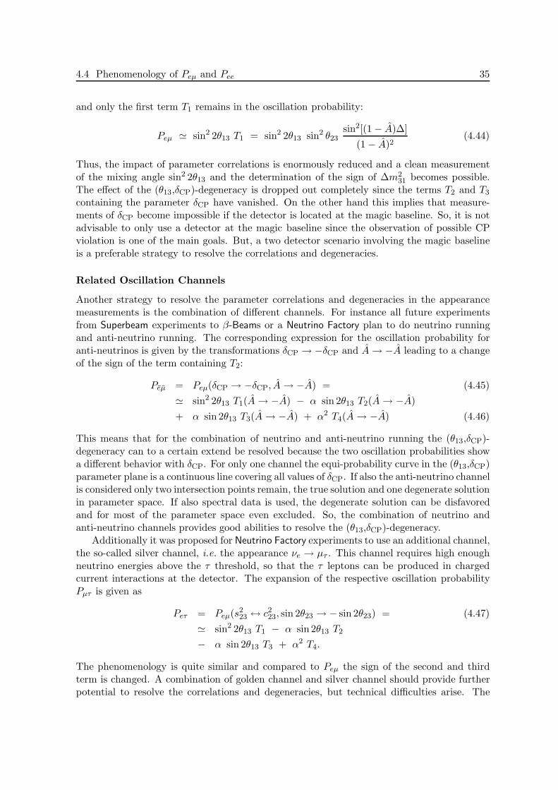
4.4 Phenomenology of Peµ and Pee 35

and only the first term T1 remains in the oscillation probability:

Peµ ≃ sin2 2θ13 T1 = sin2 2θ13 sin2 θ23sin2[(1 − A)∆]

(1 − A)2(4.44)

Thus, the impact of parameter correlations is enormously reduced and a clean measurementof the mixing angle sin2 2θ13 and the determination of the sign of ∆m2

31 becomes possible.The effect of the (θ13,δCP)-degeneracy is dropped out completely since the terms T2 and T3

containing the parameter δCP have vanished. On the other hand this implies that measure-ments of δCP become impossible if the detector is located at the magic baseline. So, it is notadvisable to only use a detector at the magic baseline since the observation of possible CPviolation is one of the main goals. But, a two detector scenario involving the magic baselineis a preferable strategy to resolve the correlations and degeneracies.

Related Oscillation Channels

Another strategy to resolve the parameter correlations and degeneracies in the appearancemeasurements is the combination of different channels. For instance all future experimentsfrom Superbeam experiments to β-Beams or a Neutrino Factory plan to do neutrino runningand anti-neutrino running. The corresponding expression for the oscillation probability foranti-neutrinos is given by the transformations δCP → −δCP and A → −A leading to a changeof the sign of the term containing T2:

Peµ = Peµ(δCP → −δCP, A → −A) = (4.45)

≃ sin2 2θ13 T1(A → −A) − α sin 2θ13 T2(A → −A)

+ α sin 2θ13 T3(A → −A) + α2 T4(A → −A) (4.46)

This means that for the combination of neutrino and anti-neutrino running the (θ13,δCP)-degeneracy can to a certain extend be resolved because the two oscillation probabilities showa different behavior with δCP. For only one channel the equi-probability curve in the (θ13,δCP)parameter plane is a continuous line covering all values of δCP. If also the anti-neutrino channelis considered only two intersection points remain, the true solution and one degenerate solutionin parameter space. If also spectral data is used, the degenerate solution can be disfavoredand for most of the parameter space even excluded. So, the combination of neutrino andanti-neutrino channels provides good abilities to resolve the (θ13,δCP)-degeneracy.

Additionally it was proposed for Neutrino Factory experiments to use an additional channel,the so-called silver channel, i.e. the appearance νe → µτ . This channel requires high enoughneutrino energies above the τ threshold, so that the τ leptons can be produced in chargedcurrent interactions at the detector. The expansion of the respective oscillation probabilityPµτ is given as

Peτ = Peµ(s223 ↔ c2

23, sin 2θ23 → − sin 2θ23) = (4.47)

≃ sin2 2θ13 T1 − α sin 2θ13 T2

− α sin 2θ13 T3 + α2 T4.

The phenomenology is quite similar and compared to Peµ the sign of the second and thirdterm is changed. A combination of golden channel and silver channel should provide furtherpotential to resolve the correlations and degeneracies, but technical difficulties arise. The

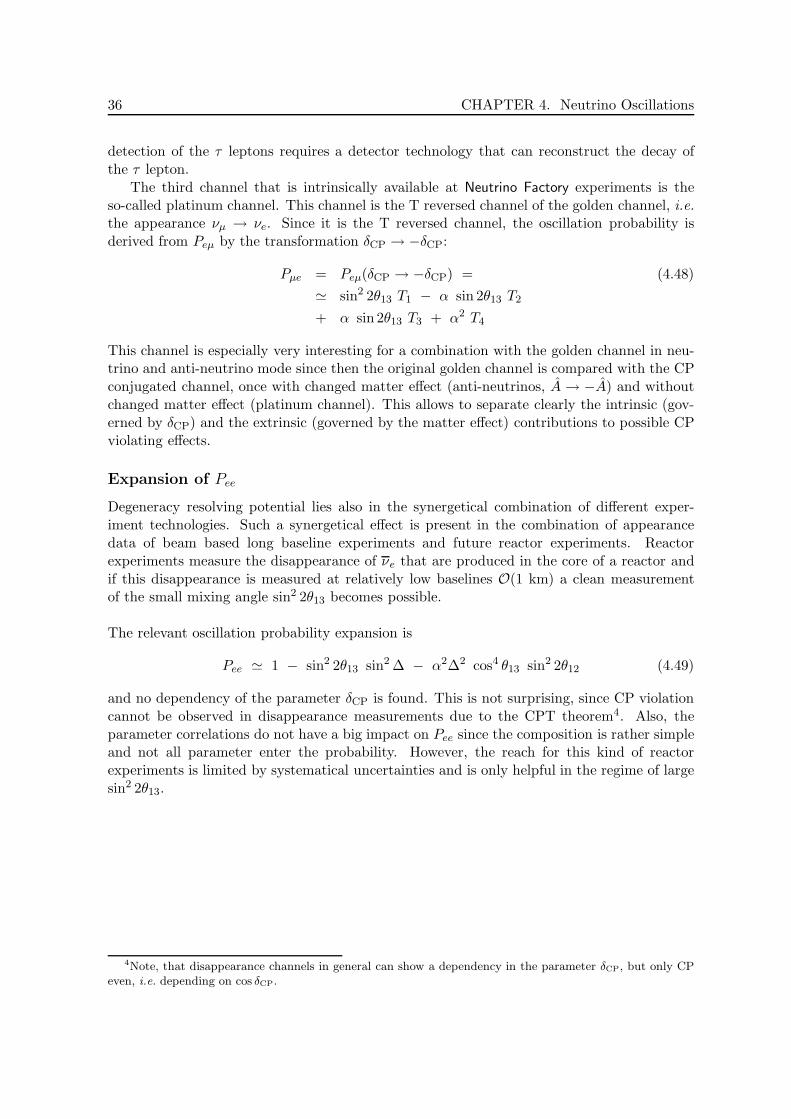
36 CHAPTER 4. Neutrino Oscillations

detection of the τ leptons requires a detector technology that can reconstruct the decay ofthe τ lepton.

The third channel that is intrinsically available at Neutrino Factory experiments is theso-called platinum channel. This channel is the T reversed channel of the golden channel, i.e.the appearance νµ → νe. Since it is the T reversed channel, the oscillation probability isderived from Peµ by the transformation δCP → −δCP:

Pµe = Peµ(δCP → −δCP) = (4.48)

≃ sin2 2θ13 T1 − α sin 2θ13 T2

+ α sin 2θ13 T3 + α2 T4

This channel is especially very interesting for a combination with the golden channel in neu-trino and anti-neutrino mode since then the original golden channel is compared with the CPconjugated channel, once with changed matter effect (anti-neutrinos, A → −A) and withoutchanged matter effect (platinum channel). This allows to separate clearly the intrinsic (gov-erned by δCP) and the extrinsic (governed by the matter effect) contributions to possible CPviolating effects.

Expansion of Pee

Degeneracy resolving potential lies also in the synergetical combination of different exper-iment technologies. Such a synergetical effect is present in the combination of appearancedata of beam based long baseline experiments and future reactor experiments. Reactorexperiments measure the disappearance of νe that are produced in the core of a reactor andif this disappearance is measured at relatively low baselines O(1 km) a clean measurementof the small mixing angle sin2 2θ13 becomes possible.

The relevant oscillation probability expansion is

Pee ≃ 1 − sin2 2θ13 sin2 ∆ − α2∆2 cos4 θ13 sin2 2θ12 (4.49)

and no dependency of the parameter δCP is found. This is not surprising, since CP violationcannot be observed in disappearance measurements due to the CPT theorem4. Also, theparameter correlations do not have a big impact on Pee since the composition is rather simpleand not all parameter enter the probability. However, the reach for this kind of reactorexperiments is limited by systematical uncertainties and is only helpful in the regime of largesin2 2θ13.

4Note, that disappearance channels in general can show a dependency in the parameter δCP, but only CPeven, i.e. depending on cos δCP.

37

Chapter 5

Neutrino Data

In this chapter we will review the current data that exists for the properties of neutrinos. Themain focus is on the confirmation of neutrino oscillations and the status of measurements ofthe neutrino oscillation parameters. But before this is discussed also different experimentalresults of measurements of neutrino properties are briefly discussed.

5.1 Number of Flavors

The LEP collider experiment has provided various precision measurements of weak interactionprocesses. One of the famous measurements involved the decay width of the Z0 boson. Themeasurement of electron positron collisions with a center of mass energy a at the resonance ofthe Z0 did not only allow for a determination of the Z0 mass but also a measurement of thenumber of neutrino flavors that are active in the weak interactions and couple to the Z0. Themeasured total decay width Γtot was compared to the partial width of the Z0 decay into thecharged leptons and quarks, the so-called visible width Γvis. The missing part of the decaywidth that was invisible to the detector Γinv = Γtot−Γvis = 498±4.2 MeV could be comparedwith the expected Standard Model decay width of the decay into neutrinos Z0 → νανα andthe number of light neutrino flavors α that participate at the weak couplings to the Z0 bosoncould be estimated in a global fit of the data of all four LEP experiments [46]:

Nν = 2.994 ± 0.012. (5.1)

There exist further data from the LEP experiments from studies of the single γ decayse+ + e− → γ + ν + ν where the above result for the number of light neutrino flavors could beconfirmed [47–50].

There also exist indirect estimates of the number of light neutrino species from cosmologi-cal considerations. The mechanism of Big Bang Nucleosynthesis is closely related with thenumber of light neutrino species that would have been relativistic at the time of Big BangNucleosynthesis. Different than the considerations from above this number would include so-called sterile neutrinos, i.e. SU(2) singlets that do not participate with the weak interactions.The comparison of Big Bang Nucleosynthesis predictions and measurements of the abun-dances of primordial light elements constrains the number of neutrino species. The newest

38 CHAPTER 5. Neutrino Data

estimates at the 2σ confidence level are Nν < 3.3 [51] and Nν < 4.4 [52]1. Due to the largeuncertainties in measurements of the primordial light elements these numbers are less reliableand as can be seen from the last number, the existence of sterile neutrinos cannot be excluded.

5.2 Absolute Mass Scale

As was pointed out in the last chapter, neutrino oscillation experiments are only sensitive tomass squared differences ∆m2 of neutrino mass eigenstates. So, although non-zero neutrinomasses are established by the observation of neutrino oscillation, no insight is gained in thequestion of the absolute mass scale of neutrinos. However, different experimental techniqueshave addressed the absolute mass scale and provided upper mass bounds while neutrinooscillation measurements allow for lower bounds on the mass of the heaviest neutrino masseigenstate via the relation mν ≥

√∆m2. In this section we summarize the efforts to constrain

the absolute mass scale of neutrinos.

Tritium Decay

The most sensitive technique for a direct search of the effective electron based neutrino mass2

is the measurement of the electron spectrum of the electrons produced in the beta decayof Tritium near the endpoint of the decay. In the case of a non-vanishing neutrino mass thewell-known beta spectrum is distorted and the statistically most significant distortion appearsvery close to the endpoint. However, collecting enough statistics near the endpoint is verydifficult since only a tiny fraction of all beta decays happens close to the endpoint. The choiceof Tritium as the source is connected to the fact that Tritium is the isotope with the secondlowest endpoint energy E0 of all known unstable beta decaying isotopes with E0 = 18.6 keVand the fraction of beta decays close to the endpoint is proportional to 1/E3

0 , so low E0 ispreferable. The relevant process is

3H → 3He+ e− + νe (5.2)

and the effective electron based neutrino mass is given as

m2νe

=∑

k

|Uek|2m2k. (5.3)

From this formula it can be read off that the effective electron based neutrino mass is inde-pendent of the question whether neutrinos are Dirac or Majorana particles.

The first measurements in the early 1990’s observed an enhancement of beta decays nearthe endpoint rather than the expected reduction due to a non-zero neutrino mass and themeasurement provided unphysical results with m2

νe< 0. However, this problem is almost

disappeared at newer experiments due to a better understanding of the systematical uncer-tainties and improved experimental setups, mainly by an improvement of the spectrometry.

1The latter number is based on a reanalysis of the data of the measurements of the abundance of primordial4He that indicate a higher statistical uncertainty and a shift of the best-fit value [53].

2Note, that the here discussed mass bounds have been obtained in the kinematics of interactions of theneutrino flavor eigenstates and flavor eigenstates do not have distinct masses because the mass eigenstatesdo. Although it is often used in a loose terminology, it is in principle not meaningful to discuss an “electronneutrino mass” since neutrino mixing turned out to be large.

5.2 Absolute Mass Scale 39

The current best bounds are provided by the MAINZ [54] and TROITSK [55] experiments.These still get negative m2

νeas best-fit values but the uncertainty of the measurement is well

in agreement with physical values but no hint for a non-zero mνe could be found. The currentbounds are

MAINZ: mνe < 2.2 eV at the 95% confidence level

TROITSK: mνe < 2.5 eV at the 95% confidence level

An improvement of this bound can be expected from the KATRIN [56] experiment that isplanned to gain one order of magnitude in sensitivity to mνe , which is even two orders ofmagnitude improvement in the actual observable m2

νe. This increase in sensitivity is accom-

plished by an enhancement of the luminosity of the Tritium source and an improved resolutionof the spectrometer.

Kinematical Test

The effective muon and tau based neutrino masses have been investigated directly in thekinematics of weak decays where all charged decay products have been observed and measured.The effective masses are given as

m2νµ

=∑

k

|Uµk|2m2k

m2ντ

=∑

k

|Uτk|2m2k. (5.4)

The best bound for the effective muon based neutrino mass was obtained by the measurementsof pion decays at rest π+ → µ+νµ at PSI [57]

mνµ < 190 keV at the 90% confidence level (5.5)

and the best bound for the effective tau based neutrino mass is coming from the observationof tau decays into pions τ− → 2π−π+ντ and τ− → 3π−2π+ντ at the ALEPH detector of theLEP collider experiment [58]. The obtained bound is:

mντ < 18.2 MeV at the 95% confidence level. (5.6)

Cosmology

In the early universe at temperatures T & 1 MeV the neutrinos were in thermal equilibriumwith the baryon-photon plasma via the weak interactions. When the temperature droppedbelow this value, the weak interaction froze out and the neutrinos decoupled from the plasma.While the temperature of the early universe was decreasing further, it shortly after thatdropped below the electron mass me = 0.511 MeV and the electrons and positrons annihilatedtransferring their entropy to the photon gas. Thus the temperature of the photons is increasedcompared to the temperature of the neutrinos. The relation between the neutrino and photontemperatures is given by [59]3:

Tγ

Tν=

(11

4

)1

3

≈ 1.40 (5.7)

3Note added in proof: This relation is only true in the limit of vanishing neutrino masses.

40 CHAPTER 5. Neutrino Data

The photons that were produced at that time represent the famous Cosmic Microwave Back-ground that has been discovered in 1965 [60, 61]. The present spectrum of the relic photonshas been measured in the observation of the Cosmic Microwave Background by COBE [62]and has been found to be a perfect black body spectrum with a mean temperature ofTCMB = 2.725±0.002 K [63]. Thus, the present temperature of the relic neutrinos is known tobe Tν = 1.96 K, i.e. approximately 2 · 10−4 eV, and at least one neutrino species is extremelynon-relativistic4 at present. The contribution of the neutrinos to the present day matterdensity of the universe can be expressed by the sum of the masses of light neutrino species5

Ωνh2 =

∑

i mi

94 eV(5.8)

and in order not to over close the universe the so-called Cowsik-McClelland bound [64, 65]was obtained: ∑

i

mi . 94 eV h2 (5.9)

with h = 0.72 ± 0.08 at the 68% confidence level [66].

In this case neutrinos were considered to be a good candidate for dark matter. They wouldcontribute to the so-called Hot Dark Matter since they were still relativistic at decoupling,while heavy weakly massive particles (WIMPs) that would be non-relativistic at freeze outof the thermal equilibrium are referred to as candidates for the so-called Cold Dark Matter.However, neutrinos as a dominant contribution to the dark matter content of the universewould highly affect the structure formation of the universe. The reason is the large freestreaming length of the relativistic neutrinos that would suppress the amplitudes and washout matter fluctuations at small scales while Cold Dark Matter does not suppress the smallscale fluctuations at early stages. The matter fluctuations at the relevant scales were measuredin the anisotropies of the Cosmic Microwave Background at small angles, i.e. high multipolemoments, at the Wilkinson Microwave Anisotropy Probe WMAP [67]. The presence of thefluctuations at the small scales and the amplitudes ruled out the Hot Dark Matter to form themain contribution of Dark Matter and instead the so-called ΛCDM6 model was establishedand the neutrino mass was constrained [68]. The structure amplitudes at similar physicalscales but from a very different epoch of the universe can be analyzed in the Large ScaleStructure surveys. The 2dF Galaxy Redshift Survey collected the spectra and measured theredshift of about 150 000 galaxies to analyze structure formation [69] and the neutrino massescould be constrained [70]. Especially the combination of WMAP and 2dfGRS data is a powerfultool to break parameter degeneracies associated with the Cosmic Microwave Background andespecially the sum of light neutrino masses is impressively constrained [71] to:

∑

i

mi < 1.0 eV at the 95% confidence level. (5.10)

4Due to the knowledge of the atmospheric mass squared difference, at least one neutrino mass eigenstatehas a mass m &

p

|∆m231| ≈ 0.05 eV.

5The term “light neutrinos” in this context means, that they are relativistic at decoupling.6The ΛCDM model is characterized by a flat universe with Ω = 1 where about 70% of the overall energy

density comes from a Cosmological Constant Λ and the rest comes from matter energy density, approximately25% Cold Dark Matter and 5% baryonic matter.

5.2 Absolute Mass Scale 41

There exist even stronger limits that are obtained by additionally including the Lyman-α forestdata. But since the interpretation of the data is still controversial [72], the above given limitis conservative and can be regarded as robust. Note, that the above given limit still allowsfor a quasi-degenerate mass ordering of neutrino mass eigenstates if the data from neutrinooscillations, that is discussed in the next section, is considered. It should be mentioned,that there exists an estimate of a possible future detection for

∑

i mi & 0.05 eV at the 95%confidence level in the combination of future CMB data and Large Scale Structure surveys atlow and high redshift [73].

Neutrino-less Double Beta Decay

The mechanism of neutrino-less double beta decay has been briefly discussed in Chapter3. There has been large effort to observe 0νββ processes in the last two decades usingthe high-purity sources with enriched parent isotopes as for instance 100Mo, 116Cd, 130Te,or 136Xe. The best sensitivities however could be achieved in experiments that used thegermanium isotope 76Ge as a source. The source serves simultaneously as the detector andhas to be shielded against possible background sources like for instance unidentified external γradiation. The search for 0νββ decay results in practice in the search for the decay spectrum,a sharp peak at the known Q value of the used isotope that is in the case of 76Ge a valueof Q = 2039 keV. The sensitivity of the experiment is given by the size of the source, itspurity and the level of background suppression. The best lower limit for the half-life of 0νββis currently provided from the data of the Heidelberg-Moscow experiment that used a 11 kggermanium source with an enrichment of 86% 76Ge (the natural abundance is 7.8%). Thedata taking took place in the Gran Sasso laboratories in the years 1990-2003 leading to anexposure of 53.9 kg yrs and no positive signal at the expected peak position could be foundand an upper limit for the half-life was obtained [74,75]:

T1/2 > 1.9 · 1025 yrs at the 90% confidence level. (5.11)

This can be translated into an upper bound on the effective neutrino mass matrix entry 〈mee〉by the use of the nuclear matrix elements from [76] to

〈mee〉 < 0.35 eV at the 90% confidence level (5.12)

where the uncertainties associated with the nuclear matrix elements have been taken intoaccount. A similar limit was obtained at the 76Ge experiment IGEX [77].

There exists a claim of parts of the Heidelberg-Moscow collaboration that neutrino-lessdouble beta decay could be observed in the expanded data set of 71.7 kg yrs. It is pretendedthat a peak has been found at the expected Q value with a 4.2σ significance [78] and theobtained life-time is

T1/2 = 1.19+2.99−0.50 · 1025 yrs (5.13)

which implies the evidence of neutrino-less double beta decay with the effective neutrino mass

〈mee〉 = 0.44+0.14−0.20 eV (5.14)

In this case neutrinos are Majorana particles and as can be seen from Fig. 3.5 the neutrinomass ordering would be quasi-degenerate. Not only does this claim of evidence dissent former

42 CHAPTER 5. Neutrino Data

results of Heidelberg-Moscow and IGEX but additionally the possible parameter space for thesmallest neutrino mass in the claimed region for 〈mee〉 is strongly constrained from the massbound coming from cosmology as can be read off Fig. 3.5. The claim of the evidence is verycontroversially discussed [79–84]. There exist various proposals for future 0νββ experimentswith source strengths of ∼ 100 kg that will be able to test the claim with different isotopesused as for instance CUORE (130Te) [85], GERDA (76Ge) [86,87], and MAJORANA (76Ge) [88].A good review of the topic, including a discussion of the claim of evidence and details of futureexperiments can be found in [89].

5.3 Oscillation Data

There has been a huge progress in our knowledge of neutrino properties in the last years comingfrom observations of neutrino oscillations from neutrinos coming from natural sources as thesun and the earth’s atmosphere and also from artificially produced neutrinos in completelyearth-based experiments. In this section we will briefly review the status of the neutrino datathat has been obtained from neutrino oscillation data.

Solar Data

Nuclear fusion reactions in the interior of the sun are the driving processes of the thermalenergy of the sun. The main process is the fusion of Hydrogen to Helium with a net reaction

4p+ + 2e− → 4He + 2νe. (5.15)

This net reaction is driven by various single reactions that form a reaction chain. The dom-inating reaction chain with a contribution of ∼ 98% to the sun’s energy is the so-called ppcycle. In the chain of the pp cycle five single reactions produce electron neutrinos νe of dif-ferent energies, the pp, pep, hep, 7Be and 8B neutrinos. Since all reactions in the sun arefusion reaction no anti-neutrinos are produced and additionally no muon or tau neutrinosappear in the reactions, so that the sun is a pure νe source. The neutrino energies in theneutrino spectrum of the sun are relatively small and do not exceed 11 MeV. The pep and7Be neutrinos have discrete energies whereas the other neutrinos form continuous spectra.The pp neutrinos give the main contribution to the neutrino spectrum of the sun and appearat very low energies Eν . 0.4 MeV. The theoretical predictions of the solar neutrino fluxes isgiven in the so-called Standard Model of the sun SSM [90, 91] and the theoretical spectrumof the solar neutrino flux can be found amongst further details in [92].

The first experiment that measured the neutrino flux from the sun was the Homestake [93]chlorine experiment and the neutrinos were detected in the reaction

νe + 37Cl →37 Ar + e−. (5.16)

However, the detection was not direct but after data taking the amount of produced 37Arwas estimated by radiochemical methods. The threshold of the process is 0.814 MeV andonly the 7Be, pep, and 8B neutrinos could be measured where the latter gave the maincontribution. The pp neutrinos could be detected at different radiochemical experimentsSAGE [94], GALLEX [95], and GNO [96] using 71Ga in the reaction

νe + 71Ga →71 Ge + e−. (5.17)

5.3 Oscillation Data 43

The reaction has a threshold of 0.234 MeV and is thus also sensitive to the low energypp neutrinos. Due to the small cross sections the observed neutrino rates were so smallthat a new unit had been introduced to describe the low rates, the Solar Neutrino UnitSNU≡ 10−36 ν captures per target atom and second. The Homestake experiments reported adetection of 2.56 ± 0.16 ± 0.16 SNUs [97, 98] and the later gallium experiments could collectmore statistics, i.e. 66.9+3.9+3.6

−3.8−3.2 SNUs at SAGE [94,99] and 66.9+3.9+3.6−3.8−3.2 SNUs at GALLEX/GNO

[95,96,100].

Direct measurements of solar neutrinos could be achieved at the Water Cherenkov de-tectors Kamiokande and later Super-Kamiokande [101] using the neutrino electron scatteringreaction

να + e− → να + e− (5.18)

with no physical threshold. The Water Cherenkov experiments require an energy cut Eν &

5 MeV so that they are only sensitive to the 8B neutrinos of the solar neutrino flux. The nicefeature of the Water Cherenkov technology was the possibility of directional information and itwas found that the measured neutrinos indeed are coming from the direction of the sun, whilethe radiochemical experiments could not confirm the initial source. The data sets indicateda neutrino flux deficit compared to the predictions of the solar flux from the SSM which wasreferred to as the Solar Neutrino Problem. However, the obtained ratio of detected to expectedneutrino rates was different at the different experiments and hinted to an energy dependentreduction of the νe flux because the experiments were sensitive to different energy ranges ofthe solar flux. Besides the discussion about the reliability of the theoretical predictions ofthe SSM the possible flavor transitions of the νe neutrinos was a popular attempt to explainthe Solar Neutrino Problem and the most natural mechanism was neutrino oscillations. Thepredictions of the SSM could be confirmed at the detector of the Sudbury Neutrino ObservatorySNO where not only charged-current or quasi-elastic neutrino reactions, but also the neutral-current reactions could be detected [102–104]. Since the observed amount of neutral currentreactions is sensitive to the total flux of all flavors φνe+φνµ+φντ the SNO results could confirmthe flux prediction of the SSM in the total flux of all flavors. So, flavor transitions of νe to νµ

or ντ were established as the cause of the Solar Neutrino Problem and furthermore, the flavortransition into a sterile neutrino in solar neutrino transitions could be heavily constrained.But still, the fit to the global solar data allowed for different separated allowed regions in thesin2 2θ-∆m2 parameter plane including vacuum oscillations and matter enhanced solutionswith MSW effect. It was the later described KamLAND data [105,106] that selected the truesolution, the so-called MSW Large Mixing Angle (LMA) solution and resolved the ambiguity.The best-fit values of the solar parameters from the combination of all available solar neutrinodata in a two-flavor framework are [107]:

sin2 2θsol = 0.83 ∆m2sol = 6.0 · 10−5 eV2. (5.19)

Atmospheric Data

A second natural source of neutrinos are the atmospheric neutrinos that are produced in theupper atmosphere of the earth due to scattering of cosmic rays (mainly protons). Pions areproduced in the interactions with the cosmic rays and in the decay chain of these pions the

44 CHAPTER 5. Neutrino Data

atmospheric neutrinos are produced:

π− → µ− + νµ

µ− → e− + νµ + νe

π+ → µ+ + νµ

µ+ → e+ + νµ + νe. (5.20)

Atmospheric neutrinos have been studied at the Water Cherenkov detector of Super-Kamiokande. The Water Cherenkov technology cannot distinguish neutrinos from anti-neutrinos but neutrino flavored neutrinos can be discriminated from muon neutrinos with quitegood accuracy. The flavor identification is performed by a shape analysis of the Cherenkovring of the charged current produced charged lepton, electron or muon. Since the lighterelectrons are affected more by scattering with the detector medium, the Cherenkov ring ofelectrons appears more fuzzy than the Cherenkov ring of a muon. On the other hand is itnot possible to distinguish neutrinos from anti-neutrinos at a Water Cherenkov detector. Ascan be seen from the reaction chain above, the atmospheric neutrinos should obey a distinctratio of 2:1 muon neutrino events to electron events in case of a no oscillation hypothesis. TheWater Cherenkov detector allows for a direction measurement of the incoming neutrinos andthe zenith angle dependence of the atmospheric neutrino flux was measured. The electron-likeevents showed the expected behavior and upward going and downward going neutrino fluxwas observed to be similar. The muon-like events however showed a different behavior andwhile the downward going neutrino flux was in agreement with the expectations a significantdeficit was observed in the upward going neutrino flux. This can be explained by flavor transi-tions νµ → ντ that occur while the neutrinos are traveling through the earth until observed inthe detector and tau neutrinos cannot be detected. This resulted in the famous evidence foratmospheric neutrino oscillations in 1998 by the Super-Kamiokande experiment [108] that canalso be confirmed by the Soudan [109] and MACRO [110, 111] experiments. In a newer anal-ysis the L/E dependence was analyzed carefully and a oscillatory dip was found which gavea clear signature for neutrino oscillations and other explanations of the flavor transitions likescenarios involving decoherence or neutrino decay were disfavored [112]. The atmosphericneutrino oscillations can be explained in a two-flavor framework and the obtained best-fitvalues in a fit to the Super-Kamiokande atmospheric data are [107]:

sin2 2θatm = 1.0 ∆m2atm = 2.0 · 10−3 eV2. (5.21)

KamLAND

The solar data alone could not solve the ambiguities and various separated alternative allowedregions in the parameter space survived. These regions involved pure vacuum oscillations,matter enhanced neutrino oscillations with a small or a large mixing angle. The true solutioncould be established at the reactor neutrino experiment KamLAND in Japan. The KamLANDdetector, a 1 kt Liquid scintillator detector is located at the Kamiokande site and measuresthe neutrino flux of 53 surrounding nuclear power plants at distances between 80 and 350 km,which sums up to an average baseline of about 180 km. Thus, the νe disappearance of thereactor neutrinos is measured at a baseline where the LMA solution of the fit to the solarneutrino data can be probed in a vacuum oscillation framework. In case of no oscillationsan event number of 356.2 ± 23.7 would have been expected in the data taking period from

5.3 Oscillation Data 45

March 2002 to January 2004 and a total of 258 events has been actually observed which is invery good agreement with two-flavor neutrino oscillations due to the solar LMA parameters[105, 106]. Furthermore, a spectral distortion could be found that indicates oscillatory L/Edependence [106]. The position of the KamLAND detector is not optimal since it is located at atoo large baseline, slightly of the oscillation maximum and hence it is not very sensitive to theoscillation amplitude and the precision for sin2 2θsol could not be increased compared to theprecision from solar data. The precision on ∆m2

sol on the other hand could be significantlyimproved. The KamLAND contribution to the Solar Neutrino Problem is very importantbecause before KamLAND the alternative allowed regions for the solar oscillation parameterscould not be ruled out. The best-fit values for the oscillation parameters in a two-flavor fit tothe KamLAND data are given as [107]:

sin2 2θsol = 0.83 ∆m2sol = 8.1 · 10−5 eV2. (5.22)

CHOOZ

The third mixing angle sin2 2θ13 has been addressed in the measurements of the CHOOZreactor experiment [113]. The 5 t Liquid Scintillator detector was placed at a distance ofL=1 km to the reactor cores of the Chooz reactor site. The reactor cores provide a large fluxof νe and only the disappearance channel of the electron anti-neutrinos could be performedsince the energies of reactor neutrinos are to small to produce the heavy muon or tau leptonsin charged-current reactions. However, in the data taking phase between April 1997 andJuly 1997 no hints for any neutrino oscillations could be found and an upper limit for theparameter sin2 2θ13 was published [114]. The obtained limit is strongly dependent on thechosen value of the atmospheric ∆m2

atm and for ∆m2atm < 10−3 eV2 no limit can be obtained

at all. The authors [115] of performed a global fit of the CHOOZ data with the atmosphericdata to include the constraints on ∆m2

atm into the CHOOZ limit and the obtained upper limitfor sin2 2θ13 is [107]:

sin2 2θ13 < 0.11 (0.25) at the 90% (3σ) confidence level. (5.23)

The period of data taking might seem very low and one might wonder if a longer period couldnot have improved the limit by an increased statistics. But, as will be pointed out later inChapter 6.3 reactor experiments are mainly limited by systematical uncertainties and not thecollected statistics.

K2K and MINOS

The first confirmation of the atmospheric neutrino oscillation in an earth-based experimentwas provided by the K2K [116] experiment in Japan. At K2K a conventionally produced νµ

beam was produced at the accelerator complex of KEK and lead to the Super-KamiokandeWater Cherenkov detector at a baseline of L=250 km. The mean energy of the neutrinos inthe beam was 1.3 GeV and oscillation due to the atmospheric parameters should evolve. Themechanism of conventional beam production will be discussed in Chapter 6.1. The full datasample was taken in the period from June 1999 to November 2004 and 112 νµ events have beenobserved whereas in case of no oscillations 158+9.2

−8.6 events would have been expected [117,118].The fit in a two-flavor framework implied an allowed region for sin2 2θatm and ∆m2

atm that wasvery well in agreement with the atmospheric neutrino data however no significant improvementin the precision could be achieved.

46 CHAPTER 5. Neutrino Data

In 2006 the MINOS experiment [119] in the United States published the first year results ofthe measurement of νµ neutrinos [120–123]. The experiment uses a conventionally producedνµ beam at a mean energy of 3 GeV that is produced at the FermiLab accelerator complexand directed towards the 5.4 kt Magnetized Iron Calorimeter MINOS detector located in theSoudan mine 735 km north of FermiLab. The MINOS experiment is still ongoing and a five yearrun is planned [124]. The first observed event sample contains 122 νµ events whereas in caseof no oscillations 239±17 events would have been expected. The MINOS experiment providesthe slightly better statistical significance and better energy reconstruction capabilities thanK2K and thus the precision on ∆m2

atm has slightly improved by the inclusion of the MINOSdata. Furthermore the best-fit value has shifted to slightly higher values as will be seen inthe next subsection where a global fit to all available data will be presented.

Global Fit

In the last subsections we have discussed the available data on neutrino oscillation parametersfrom measurements of the solar neutrino flux, the atmospheric neutrino flux, the measurementof reactor neutrinos at various baselines, and finally the most recent data from the firstgeneration of conventional neutrino beam experiments. Up to now, all single data sets canbe interpreted in a two-flavor framework with only two parameters, one oscillation amplitudesin2 2θ and a corresponding oscillation frequency ∆m2. The reason why no three-flavor effectshave been observed so far is the smallness of two quantities, sin2 2θ13 and the hierarchy ofthe solar and atmospheric mass squared differences α = ∆m2

sol/∆m2atm. Nevertheless there

have been various studies that try to fit all available data sets simultaneously in a global fitin the complete three-flavor framework of neutrino oscillations [107, 125–127]. Note, that byswitching from the two-flavor frameworks to the three-flavor framework the correspondencesare:

sin2 2θsol = sin2 2θ12 ∆m2sol = ∆m2

21

sin2 2θatm = sin2 2θ23 ∆m2atm = |∆m2

31|.(5.24)

The global fit studies are updated when new data sets get available and so represent the globalknowledge of neutrino oscillation parameters. Here, we will only make use of the global fitfrom [107] and the global fit best-ft values and the allowed 3σ regions are given as:

sin2 2θ12 = 0.84+0.12−0.11 ∆m2

21 = 7.9+1.0−0.8 · 10−5 eV2

sin2 2θ23 = 1.00+0.00−0.13 |∆m2

31| = 2.6+0.6−0.6 · 10−3 eV2

sin2 2θ13 = 0.000+0.154−0.000 δCP = 0+π

−π

(5.25)

If not stated otherwise, we will adopt the best-fit values of Eq. (5.25) as the true input valuesfor the oscillation parameters used in the experiment simulations in later chapters of thiswork.

LSND

A controversial result that has not been considered in the global fit given above is the data[128] of the LSND [129] experiment being the first experiment to report the observation ofneutrino oscillation appearance. In the neutrinos coming from pion decays at rest and a Liquid

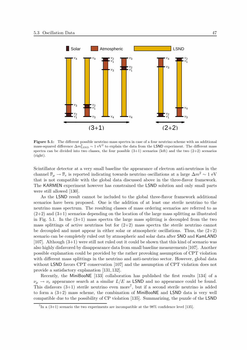
5.3 Oscillation Data 47

H3+1L H2+2L

Solar Atmospheric LSND

Ν1Ν2

Ν3

Ν4

Ν1Ν2

Ν3

Ν4Ν1Ν2

Ν3

Ν4

Ν1Ν2

Ν3

Ν4 Ν1Ν2

Ν3

Ν4Ν1Ν2

Ν3

Ν4

Figure 5.1: The different possible neutrino mass spectra in case of a four neutrino scheme with an additionalmass-squared difference ∆m2

LSND ∼ 1 eV2 to explain the data from the LSND experiment. The different massspectra can be divided into two classes, the four possible (3+1) scenarios (left) and the two (2+2) scenarios(right).

Scintillator detector at a very small baseline the appearance of electron anti-neutrinos in thechannel νµ → νe is reported indicating towards neutrino oscillations at a large ∆m2 ∼ 1 eVthat is not compatible with the global data discussed above in the three-flavor framework.The KARMEN experiment however has constrained the LSND solution and only small partswere still allowed [130].

As the LSND result cannot be included to the global three-flavor framework additionalscenarios have been proposed. One is the addition of at least one sterile neutrino to theneutrino mass spectrum. The resulting classes of mass ordering scenarios are referred to as(2+2) and (3+1) scenarios depending on the location of the large mass splitting as illustratedin Fig. 5.1. In the (3+1) mass spectra the large mass splitting is decoupled from the twomass splittings of active neutrinos but for (2+2) mass spectra the sterile neutrino cannotbe decoupled and must appear in either solar or atmospheric oscillations. Thus, the (2+2)scenario can be completely ruled out by atmospheric and solar data after SNO and KamLAND[107]. Although (3+1) were still not ruled out it could be shown that this kind of scenario wasalso highly disfavored by disappearance data from small baseline measurements [107]. Anotherpossible explanation could be provided by the rather provoking assumption of CPT violationwith different mass splittings in the neutrino and anti-neutrino sector. However, global datawithout LSND favors CPT conservation [107] and the assumption of CPT violation does notprovide a satisfactory explanation [131,132].

Recently, the MiniBooNE [133] collaboration has published the first results [134] of aνµ → νe appearance search at a similar L/E as LSND and no appearance could be found.This disfavors (3+1) sterile neutrino even more7, but if a second sterile neutrino is addedto form a (3+2) mass scheme, the combination of MiniBooNE and LSND data is very wellcompatible due to the possibility of CP violation [135]. Summarizing, the puzzle of the LSND

7In a (3+1) scenario the two experiments are incompatible at the 98% confidence level [135].

48 CHAPTER 5. Neutrino Data

result is not resolved by the recent MiniBooNE data and the νµ → νe data of MiniBooNE isrequired for the final conclusion. The LSND result will not be considered for the simulationsthroughout this work and we will only operate in a three-flavor framework with the assumptionof CPT conservation.

49

Chapter 6

Long Baseline Experiment

Scenarios

The first cognitions in neutrino oscillation physics came from the detection of neutrinos fromnatural neutrino sources like neutrinos produced in the fusion reactions in the sun’s inte-rior or neutrinos produced in the earth’s upper atmosphere. This resulted in pinning downthe leading oscillation parameters. However, observing three-flavor effects in oscillations ofneutrinos from these natural sources is hardly achievable1. So, the future of neutrino oscil-lation physics will be dominated by artificially produced “man-made” neutrinos in presentand future experiments. The era of neutrino oscillation long baseline experiments has alreadybeen initiated with the first generation of conventional neutrino beam experiments that arecurrently ongoing or finished data taking. However, these experiments were mainly plannedto measure and confirm the former measurements of the leading oscillation parameters. Al-though, it was shown that already the conventional beam experiments have some potentialto discover three flavor effects such as the observation of a non-zero sin2 2θ13 if it is justaround the corner slightly below the Chooz bound [136–141], the conventional beam exper-iments cannot constrain the parameter space of the CP phase or determine the underlyingneutrino mass hierarchy. So, new classes of experiments have been proposed to address theseissues in the future, going from Superbeam experiments that are upgrades of the conventionaltechnology to even more dedicated technologies such as β-Beam or Neutrino Factory experi-ments. In this chapter we will introduce the possible different configurations of technologies,beginning with the concept of the conventional beam based experiments and their possibleupgrade scenarios, the Superbeam experiments. The most sophisticated scenarios of β-Beamexperiments and Neutrino Factory experiments will be described in greater detail since theirperformance and optimization issues are the main topic of the following chapters where wepresent the main results. Furthermore the basic principles of reactor oscillation experimentsare reviewed because reactor experiments can play an important role, when the global pictureof future neutrino oscillation physics is discussed in Chapter 9. Additionally we will give abrief description of the rather novel idea of neutrino beam experiments with monochromaticneutrinos from electron capture processes since the technology is related to the principles ofβ-Beam experiments.

1However, there is some potential to extract information on sin2 2θ13 from atmospheric neutrino data [17].

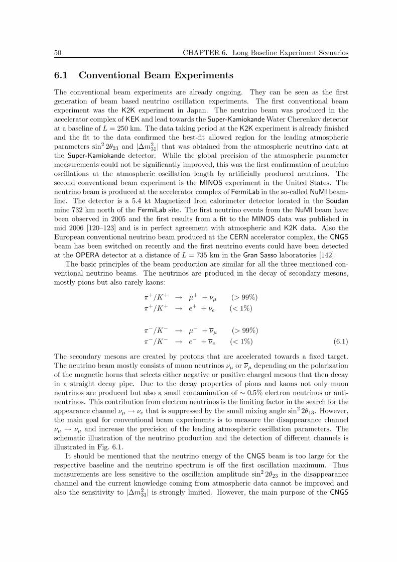
50 CHAPTER 6. Long Baseline Experiment Scenarios

6.1 Conventional Beam Experiments

The conventional beam experiments are already ongoing. They can be seen as the firstgeneration of beam based neutrino oscillation experiments. The first conventional beamexperiment was the K2K experiment in Japan. The neutrino beam was produced in theaccelerator complex of KEK and lead towards the Super-Kamiokande Water Cherenkov detectorat a baseline of L = 250 km. The data taking period at the K2K experiment is already finishedand the fit to the data confirmed the best-fit allowed region for the leading atmosphericparameters sin2 2θ23 and |∆m2

31| that was obtained from the atmospheric neutrino data atthe Super-Kamiokande detector. While the global precision of the atmospheric parametermeasurements could not be significantly improved, this was the first confirmation of neutrinooscillations at the atmospheric oscillation length by artificially produced neutrinos. Thesecond conventional beam experiment is the MINOS experiment in the United States. Theneutrino beam is produced at the accelerator complex of FermiLab in the so-called NuMI beam-line. The detector is a 5.4 kt Magnetized Iron calorimeter detector located in the Soudanmine 732 km north of the FermiLab site. The first neutrino events from the NuMI beam havebeen observed in 2005 and the first results from a fit to the MINOS data was published inmid 2006 [120–123] and is in perfect agreement with atmospheric and K2K data. Also theEuropean conventional neutrino beam produced at the CERN accelerator complex, the CNGSbeam has been switched on recently and the first neutrino events could have been detectedat the OPERA detector at a distance of L = 735 km in the Gran Sasso laboratories [142].

The basic principles of the beam production are similar for all the three mentioned con-ventional neutrino beams. The neutrinos are produced in the decay of secondary mesons,mostly pions but also rarely kaons:

π+/K+ → µ+ + νµ (> 99%)

π+/K+ → e+ + νe (< 1%)

π−/K− → µ− + νµ (> 99%)

π−/K− → e− + νe (< 1%) (6.1)

The secondary mesons are created by protons that are accelerated towards a fixed target.The neutrino beam mostly consists of muon neutrinos νµ or νµ depending on the polarizationof the magnetic horns that selects either negative or positive charged mesons that then decayin a straight decay pipe. Due to the decay properties of pions and kaons not only muonneutrinos are produced but also a small contamination of ∼ 0.5% electron neutrinos or anti-neutrinos. This contribution from electron neutrinos is the limiting factor in the search for theappearance channel νµ → νe that is suppressed by the small mixing angle sin2 2θ13. However,the main goal for conventional beam experiments is to measure the disappearance channelνµ → νµ and increase the precision of the leading atmospheric oscillation parameters. Theschematic illustration of the neutrino production and the detection of different channels isillustrated in Fig. 6.1.

It should be mentioned that the neutrino energy of the CNGS beam is too large for therespective baseline and the neutrino spectrum is off the first oscillation maximum. Thusmeasurements are less sensitive to the oscillation amplitude sin2 2θ23 in the disappearancechannel and the current knowledge coming from atmospheric data cannot be improved andalso the sensitivity to |∆m2

31| is strongly limited. However, the main purpose of the CNGS

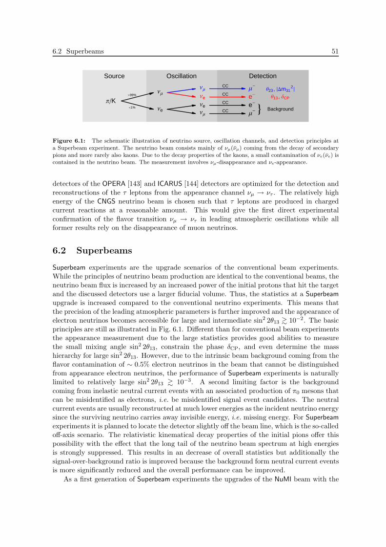
6.2 Superbeams 51

Source Oscillation Detection

ΝΜ

ΠKΝe

ΝΜ

Νe

ΝeΝΜ

Μ-

e-

e-

Μ-

CC

CC

CC

CC < Background

Θ23 , ÈDm312È

Θ13 , ∆CP>99%

<1%

Figure 6.1: The schematic illustration of neutrino source, oscillation channels, and detection principles ata Superbeam experiment. The neutrino beam consists mainly of νµ(νµ) coming from the decay of secondarypions and more rarely also kaons. Due to the decay properties of the kaons, a small contamination of νe(νe) iscontained in the neutrino beam. The measurement involves νµ-disappearance and νe-appearance.

detectors of the OPERA [143] and ICARUS [144] detectors are optimized for the detection andreconstructions of the τ leptons from the appearance channel νµ → ντ . The relatively highenergy of the CNGS neutrino beam is chosen such that τ leptons are produced in chargedcurrent reactions at a reasonable amount. This would give the first direct experimentalconfirmation of the flavor transition νµ → ντ in leading atmospheric oscillations while allformer results rely on the disappearance of muon neutrinos.

6.2 Superbeams

Superbeam experiments are the upgrade scenarios of the conventional beam experiments.While the principles of neutrino beam production are identical to the conventional beams, theneutrino beam flux is increased by an increased power of the initial protons that hit the targetand the discussed detectors use a larger fiducial volume. Thus, the statistics at a Superbeamupgrade is increased compared to the conventional neutrino experiments. This means thatthe precision of the leading atmospheric parameters is further improved and the appearance ofelectron neutrinos becomes accessible for large and intermediate sin2 2θ13 & 10−2. The basicprinciples are still as illustrated in Fig. 6.1. Different than for conventional beam experimentsthe appearance measurement due to the large statistics provides good abilities to measurethe small mixing angle sin2 2θ13, constrain the phase δCP, and even determine the masshierarchy for large sin2 2θ13. However, due to the intrinsic beam background coming from theflavor contamination of ∼ 0.5% electron neutrinos in the beam that cannot be distinguishedfrom appearance electron neutrinos, the performance of Superbeam experiments is naturallylimited to relatively large sin2 2θ13 & 10−3. A second limiting factor is the backgroundcoming from inelastic neutral current events with an associated production of π0 mesons thatcan be misidentified as electrons, i.e. be misidentified signal event candidates. The neutralcurrent events are usually reconstructed at much lower energies as the incident neutrino energysince the surviving neutrino carries away invisible energy, i.e. missing energy. For Superbeamexperiments it is planned to locate the detector slightly off the beam line, which is the so-calledoff-axis scenario. The relativistic kinematical decay properties of the initial pions offer thispossibility with the effect that the long tail of the neutrino beam spectrum at high energiesis strongly suppressed. This results in an decrease of overall statistics but additionally thesignal-over-background ratio is improved because the background form neutral current eventsis more significantly reduced and the overall performance can be improved.

As a first generation of Superbeam experiments the upgrades of the NuMI beam with the

52 CHAPTER 6. Long Baseline Experiment Scenarios

Superbeam experiment NOνA [145] in the United States and the T2K [146] experiment inJapan are proposed. The second generation of Superbeam experiments is planned to evenincrease the performance of Superbeams by further increasing statistics and neutrino energies.So, it is proposed to use a megaton Water Cherenkov detector such as the possible to be builtHyper-Kamiokande detector [146] in Japan or MEMPHYS [147] in Europe. The respectiveSuperbeam experiments are the T2HK experiments and the SPL Superbeam [148]. Also at theFermiLab it is proposed to upgrade the first generation Superbeam experiment NOνA with anupgraded proton driver [149].

6.3 Reactor Experiments

It was already mentioned that the observation of νe disappearance in the neutrino flux pro-duced in fission reactions (mainly 235U fission processes) in the core of a reactor provides theopportunity to examine neutrino oscillation properties. The neutrinos are detected in theinverse beta decay

νe + p → e+ + n (6.2)

with a threshold of approximately 1.8 MeV and a significant signal signature that allows toreconstruct the incident neutrino energy due to the coincidence of three photons, the twoprompt photons from the incident annihilation of the positron and the a delayed photon fromthe capture of the neutron.

The first observation of neutrino events was performed at a early reactor experiment in1956 and was followed by neutrino oscillation experiments at very low baseline L . 100 mthat did not find any hints for νe disappearance at this distances. The most important werethe experiments at Gosgen [150], Bugey [151], Palo Verde [152], and CHOOZ [113].

If the detector is located at a distance L ∼ 100 km the measurement is sensitive to theleading solar parameters sin2 2θ12 and ∆m2

21. The ongoing KamLAND experiment in Japanmeasures the νe disappearance at a 1 kt Liquid Scintillator detector that are coming from53 surrounding power plants at an average distance of L∼ 180 km. Although this distance isslightly of the solar oscillation maximum, the KamLAND data [105, 106] established a disap-pearance that was consistent with the LMA-MSW solution of the solar neutrino data. Due tothe inefficient location of the detector, KamLAND is less sensitive to the oscillation amplitudesin2 2θ23 but could provide a good measurement of ∆m2

21. For precision measurements ofboth parameters it has been proposed to use a very large Liquid Scintillator detector like forinstance the LENA [153,154] detector (50 kt) at a baseline of L ∼ 60 km to perform precisionmeasurements of the solar parameters at the percent level.

The Liquid Scintillator can also be located at the first atmospheric oscillation maximumL ∼ 1.3 km to search for νe disappearance in oscillations at the atmospheric frequency. Thisoscillation channel is driven by the small mixing angle sin2 2θ13 at this baselines and a cleanmeasurement of sin2 2θ13 becomes possible because only few parameter correlations spoil thisoscillation channel compared to the appearance channels at beam based experiments. Thelimiting factor at sin2 2θ13 reactor experiments is the issue of systematical uncertainties [155].In this close distance from the reactor core statistics is not that kind of a problem because theneutrino flux is extremely high. But systematical uncertainties such as the uncertainties incross sections, the uncertainty of the normalization of the neutrino flux, and the uncertaintyof the fiducial mass of the detector can easily destroy the sensitivity to sin2 2θ13. It is crucialto keep the overall systematical uncertainties below the level of 1% which can be achieved by a

6.4 Electron Capture Beams 53

Source Oscillation Detection

235U Ν

e Ν

e 8e+

® ΓAnnihilation

n ® ΓCapture

CC Θ13

Figure 6.2: The schematic illustration of neutrino source, oscillation channels, and detection principles at aneutrino reactor experiment. The νe are produced in the fission reactions of nuclei (mainly 235U) in a reactorcore. The disappearance of the νe is measured.

combined measurement at a near and a far detector so that associated uncertainties cancel out.The schematic illustration of this kind of neutrino oscillation experiment is shown in Fig. 6.2.

Still, the CHOOZ bound gives the current upper limit (slightly improved by solar data) forsin2 2θ13 but no hint for disappearance could be observed. However, the CHOOZ experimentonly used a far detector and was highly limited by the systematical uncertainties. All futureplanned reactor experiments are proposed as multi-detector setups to increase the sin2 2θ13

sensitivities to smaller values of sin2 2θ13. The first of the new generation of sin2 2θ13 reactorexperiments is DoubleCHOOZ [156] with two detectors at the same Chooz reactor complex asthe initial CHOOZ experiment. The total exposure of a reactor experiment is proportional toand can be described by the product of the runtime, the detector mass, and the thermal powerof the reactor core, i.e. the so-called integrated luminosity. The exposure of the DoubleCHOOZexperiment is planned as 5 yrs × 10.16 t × 8.4 GW ∼ 430 GW t yrs. However, to evenimprove the sensitivity to sin2 2θ13 even larger reactor experiments have been proposed withan integrated Luminosity of the order of 104 GW t yrs [157]. For such experiments at thishigh exposure the handling of bin-to-bin uncorrelated systematical uncertainties have to becarefully addressed to further improve the sensitivity to sin2 2θ13. This is discussed for atypical scenario in [155] there called Reactor-II scenario. Possible realizations are the proposedreactor experiments Daya Bay [158] in China, RENO [159] in Korea, KASKA-II [160] in Japan,or even an upgrade at the Chooz site TripleCHOOZ [161].

6.4 Electron Capture Beams

Recently, another idea has been proposed, which makes use of a neutrino beam with neutrinoscoming from electron capture processes [162–168]. The electron neutrinos that are emittedfrom such electron capture processes would have a definite monochromatic energy Q in the restframe of the mother nuclei. Therefore by accelerating the mother nuclei to a Lorentz factor γthe neutrino energy Eν can be completely controlled, since the energy of the neutrinos thatare boosted exactly towards the direction of the detector is Eν = 2γQ. The challenge from atechnological point of view is that simultaneously a beam of electrons has to be acceleratedat the same γ and coincide in the decay ring at one point with the accelerated nuclei so thatboth are in the same rest frame and the electron capture process can occur.

In such a scenario, the γ factor and the baseline length L have to be chosen respectivelyto the Q value of the electron capture process, the location of the oscillation maximum,and the minimal energy observable at the detector, e.g. above the Cherenkov threshold of

54 CHAPTER 6. Long Baseline Experiment Scenarios

muons at a Water Cherenkov detector. For example, if Q is relatively large (O(1 MeV)),γ can be chosen to be of the order O(100). In this case the neutrino beam can be viewedas exactly monoenergetic in the detector [162–169]. On the contrary, if Q is relatively small(O(100 keV)) the γ must be chosen quite high (O(1000)), but the necessary choice of thebaseline leads to the effect that the neutrinos now have a wider energy range at the detector.While the maximal energy of Eν = 2γQ is reached by the neutrinos in the beam axis, theenergy of the neutrinos becomes smaller off the axis and the minimal energy of the neutrinosdepends on the detector size and the baseline.

Eν(R) =Q

γ

[

1 − β√

1 + (R/L)2

]−1

≈ 2γQ

1 + (γR/L)2. (6.3)

In this scenario, the neutrino energy can be reconstructed from the measurement of the verticalposition R relatively to the beam axis within the detector and a superb energy resolution canbe achieved [162, 163, 170]2. This case seems interesting since only with one accelerationfactor γ a wide range of neutrino energy can be covered simultaneously with a very accurateneutrino energy determination. On the other hand only neutrino running is available andno comparison with the anti-neutrino channel is possible, hence parameter correlations andespecially the eight-fold degeneracy is hard to be resolved. The lack of the anti-neutrinochannel has to be compensated by the extraordinary energy resolution available and enoughstatistics has to be collected, i.e. a very large fiducial mass such as at a megaton WaterCherenkov detector is preferable. The performance of such high γ electron capture beamexperiments was analyzed in [170] and the requirements for being competitive to a standardNeutrino Factory experiment was estimated. The considered electron capture process was

11050 Sn + e− → 110

49 In + νe. (6.4)

with a rest frame neutrino energy of Q = 267 keV at a lifetime of 4.11 h. It was foundthat in principle the very good energy resolution abilities can provide the potential to resolvethe eight-fold degeneracy and measurements of sin2 2θ13 and δCP in a very large part of theparameter space can be possible. Even a competitiveness to a Neutrino Factory or β-Beamscould be given however the requirements turned out to be extreme. The acceleration factor isrequired to be γ & 2000 which would need a very powerful accelerator complex of the size ofthe LHC and the high statistics to gain from the superb energy resolution capabilities wouldrequire a very high number of electron capture decays per year ∼ 1018 which is hardly feasibleconsidered that the lifetime is 4.11 h in the rest frame of the process3.

6.5 Beta Beams

The idea of producing a flavor pure electron neutrino beam in the beta decay of acceleratedmother nuclei was first proposed in [175]. In the last years this idea has gained a reasonablepopularity and is discussed as the neutrino source of a possible future neutrino oscillationexperiment, the so-called β-Beam. Various papers have been published discussing different

2The position reconstruction of the initial vertex at a Water Cherenkov detector is possible at least at aresolution of 30 cm [171]

3The rate of electron capture processes clearly requires enhancement which could be achieved by a laserirradiation as discussed in [172–174].

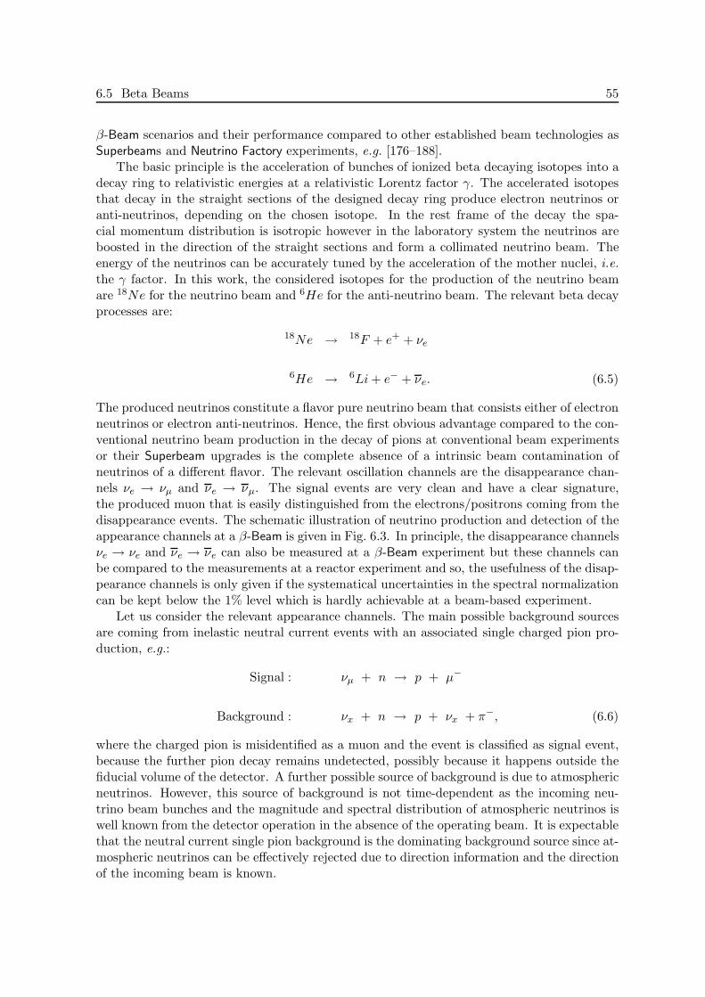
6.5 Beta Beams 55

β-Beam scenarios and their performance compared to other established beam technologies asSuperbeams and Neutrino Factory experiments, e.g. [176–188].

The basic principle is the acceleration of bunches of ionized beta decaying isotopes into adecay ring to relativistic energies at a relativistic Lorentz factor γ. The accelerated isotopesthat decay in the straight sections of the designed decay ring produce electron neutrinos oranti-neutrinos, depending on the chosen isotope. In the rest frame of the decay the spa-cial momentum distribution is isotropic however in the laboratory system the neutrinos areboosted in the direction of the straight sections and form a collimated neutrino beam. Theenergy of the neutrinos can be accurately tuned by the acceleration of the mother nuclei, i.e.the γ factor. In this work, the considered isotopes for the production of the neutrino beamare 18Ne for the neutrino beam and 6He for the anti-neutrino beam. The relevant beta decayprocesses are:

18Ne → 18F + e+ + νe

6He → 6Li + e− + νe. (6.5)

The produced neutrinos constitute a flavor pure neutrino beam that consists either of electronneutrinos or electron anti-neutrinos. Hence, the first obvious advantage compared to the con-ventional neutrino beam production in the decay of pions at conventional beam experimentsor their Superbeam upgrades is the complete absence of a intrinsic beam contamination ofneutrinos of a different flavor. The relevant oscillation channels are the disappearance chan-nels νe → νµ and νe → νµ. The signal events are very clean and have a clear signature,the produced muon that is easily distinguished from the electrons/positrons coming from thedisappearance events. The schematic illustration of neutrino production and detection of theappearance channels at a β-Beam is given in Fig. 6.3. In principle, the disappearance channelsνe → νe and νe → νe can also be measured at a β-Beam experiment but these channels canbe compared to the measurements at a reactor experiment and so, the usefulness of the disap-pearance channels is only given if the systematical uncertainties in the spectral normalizationcan be kept below the 1% level which is hardly achievable at a beam-based experiment.

Let us consider the relevant appearance channels. The main possible background sourcesare coming from inelastic neutral current events with an associated single charged pion pro-duction, e.g.:

Signal : νµ + n → p + µ−

Background : νx + n → p + νx + π−, (6.6)

where the charged pion is misidentified as a muon and the event is classified as signal event,because the further pion decay remains undetected, possibly because it happens outside thefiducial volume of the detector. A further possible source of background is due to atmosphericneutrinos. However, this source of background is not time-dependent as the incoming neu-trino beam bunches and the magnitude and spectral distribution of atmospheric neutrinos iswell known from the detector operation in the absence of the operating beam. It is expectablethat the neutral current single pion background is the dominating background source since at-mospheric neutrinos can be effectively rejected due to direction information and the directionof the incoming beam is known.

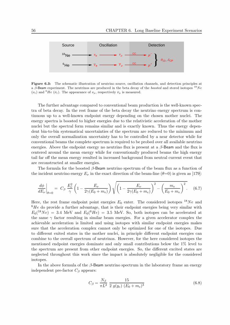
56 CHAPTER 6. Long Baseline Experiment Scenarios

Source Oscillation Detection

Νe18Ne

6He Ν

e

ΝΜ

Ν

Μ

Μ-

Μ+

CC

CC < Θ13, ∆CP

Figure 6.3: The schematic illustration of neutrino source, oscillation channels, and detection principles ata β-Beam experiment. The neutrinos are produced in the beta decay of the boosted and stored isotopes 18Ne(νe) and 6He (νe). The appearance of νµ, respectively νµ is measured.

The further advantage compared to conventional beam production is the well-known spec-tra of beta decay. In the rest frame of the beta decay the neutrino energy spectrum is con-tinuous up to a well-known endpoint energy depending on the chosen mother nuclei. Theenergy spectra is boosted to higher energies due to the relativistic acceleration of the mothernuclei but the spectral form remains similar and is exactly known. Thus the energy depen-dent bin-to-bin systematical uncertainties of the spectrum are reduced to the minimum andonly the overall normalization uncertainty has to be controlled by a near detector while forconventional beams the complete spectrum is required to be probed over all available neutrinoenergies. Above the endpoint energy no neutrino flux is present at a β-Beam and the flux iscentered around the mean energy while for conventionally produced beams the high energytail far off the mean energy resulted in increased background from neutral current event thatare reconstructed at smaller energies.

The formula for the boosted β-Beam neutrino spectrum of the beam flux as a function ofthe incident neutrino energy Eν in the exact direction of the beam-line (θ=0) is given as [179]:

dφ

dEν

∣∣∣∣θ=0

= CβE2

ν

γ

(

1 − Eν

2γ(E0 + me)

)√(

1 − Eν

2γ(E0 + me)

)2

−(

me

E0 + me

)2

. (6.7)

Here, the rest frame endpoint point energies E0 enter. The considered isotopes 18Ne and6He do provide a further advantage, that is their endpoint energies being very similar withE0(

18Ne) = 3.4 MeV and E0(6He) = 3.5 MeV. So, both isotopes can be accelerated at

the same γ factor resulting in similar beam energies. For a given accelerator complex theachievable acceleration is limited and using isotopes with similar endpoint energies makessure that the acceleration complex cannot only be optimized for one of the isotopes. Dueto different exited states in the mother nuclei, in principle different endpoint energies cancombine to the overall spectrum of neutrinos. However, for the here considered isotopes thementioned endpoint energies dominate and only small contributions below the 1% level tothe spectrum are present from other endpoint energies. So, the different excited states areneglected throughout this work since the impact is absolutely negligible for the consideredisotopes.

In the above formula of the β-Beam neutrino spectrum in the laboratory frame an energyindependent pre-factor Cβ appears:

Cβ =Nβ

πL2

15

2 g(ye) (E0 + me)3(6.8)

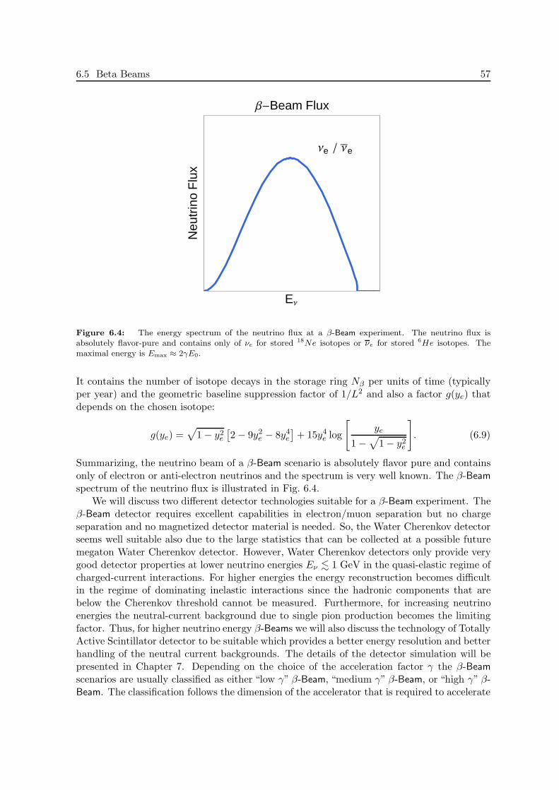
6.5 Beta Beams 57

EΝ

Neu

trin

oF

lux

Β-Beam Flux

Νe Ν

e

Figure 6.4: The energy spectrum of the neutrino flux at a β-Beam experiment. The neutrino flux isabsolutely flavor-pure and contains only of νe for stored 18Ne isotopes or νe for stored 6He isotopes. Themaximal energy is Emax ≈ 2γE0.

It contains the number of isotope decays in the storage ring Nβ per units of time (typicallyper year) and the geometric baseline suppression factor of 1/L2 and also a factor g(ye) thatdepends on the chosen isotope:

g(ye) =√

1 − y2e

[2 − 9y2

e − 8y4e

]+ 15y4

e log

[

ye

1 −√

1 − y2e

]

. (6.9)

Summarizing, the neutrino beam of a β-Beam scenario is absolutely flavor pure and containsonly of electron or anti-electron neutrinos and the spectrum is very well known. The β-Beamspectrum of the neutrino flux is illustrated in Fig. 6.4.

We will discuss two different detector technologies suitable for a β-Beam experiment. Theβ-Beam detector requires excellent capabilities in electron/muon separation but no chargeseparation and no magnetized detector material is needed. So, the Water Cherenkov detectorseems well suitable also due to the large statistics that can be collected at a possible futuremegaton Water Cherenkov detector. However, Water Cherenkov detectors only provide verygood detector properties at lower neutrino energies Eν . 1 GeV in the quasi-elastic regime ofcharged-current interactions. For higher energies the energy reconstruction becomes difficultin the regime of dominating inelastic interactions since the hadronic components that arebelow the Cherenkov threshold cannot be measured. Furthermore, for increasing neutrinoenergies the neutral-current background due to single pion production becomes the limitingfactor. Thus, for higher neutrino energy β-Beams we will also discuss the technology of TotallyActive Scintillator detector to be suitable which provides a better energy resolution and betterhandling of the neutral current backgrounds. The details of the detector simulation will bepresented in Chapter 7. Depending on the choice of the acceleration factor γ the β-Beamscenarios are usually classified as either “low γ” β-Beam, “medium γ” β-Beam, or “high γ” β-Beam. The classification follows the dimension of the accelerator that is required to accelerate

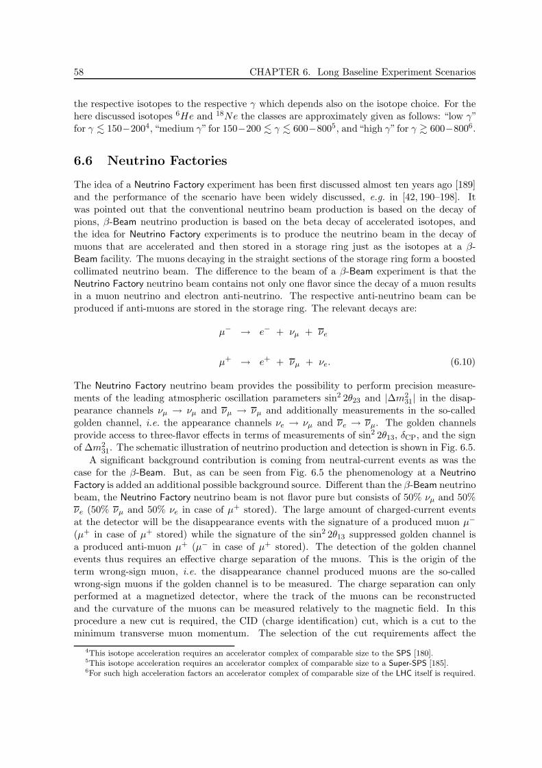
58 CHAPTER 6. Long Baseline Experiment Scenarios

the respective isotopes to the respective γ which depends also on the isotope choice. For thehere discussed isotopes 6He and 18Ne the classes are approximately given as follows: “low γ”for γ . 150−2004, “medium γ” for 150−200 . γ . 600−8005, and“high γ”for γ & 600−8006.

6.6 Neutrino Factories

The idea of a Neutrino Factory experiment has been first discussed almost ten years ago [189]and the performance of the scenario have been widely discussed, e.g. in [42, 190–198]. Itwas pointed out that the conventional neutrino beam production is based on the decay ofpions, β-Beam neutrino production is based on the beta decay of accelerated isotopes, andthe idea for Neutrino Factory experiments is to produce the neutrino beam in the decay ofmuons that are accelerated and then stored in a storage ring just as the isotopes at a β-Beam facility. The muons decaying in the straight sections of the storage ring form a boostedcollimated neutrino beam. The difference to the beam of a β-Beam experiment is that theNeutrino Factory neutrino beam contains not only one flavor since the decay of a muon resultsin a muon neutrino and electron anti-neutrino. The respective anti-neutrino beam can beproduced if anti-muons are stored in the storage ring. The relevant decays are:

µ− → e− + νµ + νe

µ+ → e+ + νµ + νe. (6.10)

The Neutrino Factory neutrino beam provides the possibility to perform precision measure-ments of the leading atmospheric oscillation parameters sin2 2θ23 and |∆m2

31| in the disap-pearance channels νµ → νµ and νµ → νµ and additionally measurements in the so-calledgolden channel, i.e. the appearance channels νe → νµ and νe → νµ. The golden channelsprovide access to three-flavor effects in terms of measurements of sin2 2θ13, δCP, and the signof ∆m2

31. The schematic illustration of neutrino production and detection is shown in Fig. 6.5.

A significant background contribution is coming from neutral-current events as was thecase for the β-Beam. But, as can be seen from Fig. 6.5 the phenomenology at a NeutrinoFactory is added an additional possible background source. Different than the β-Beam neutrinobeam, the Neutrino Factory neutrino beam is not flavor pure but consists of 50% νµ and 50%νe (50% νµ and 50% νe in case of µ+ stored). The large amount of charged-current eventsat the detector will be the disappearance events with the signature of a produced muon µ−

(µ+ in case of µ+ stored) while the signature of the sin2 2θ13 suppressed golden channel isa produced anti-muon µ+ (µ− in case of µ+ stored). The detection of the golden channelevents thus requires an effective charge separation of the muons. This is the origin of theterm wrong-sign muon, i.e. the disappearance channel produced muons are the so-calledwrong-sign muons if the golden channel is to be measured. The charge separation can onlyperformed at a magnetized detector, where the track of the muons can be reconstructedand the curvature of the muons can be measured relatively to the magnetic field. In thisprocedure a new cut is required, the CID (charge identification) cut, which is a cut to theminimum transverse muon momentum. The selection of the cut requirements affect the

4This isotope acceleration requires an accelerator complex of comparable size to the SPS [180].5This isotope acceleration requires an accelerator complex of comparable size to a Super-SPS [185].6For such high acceleration factors an accelerator complex of comparable size of the LHC itself is required.

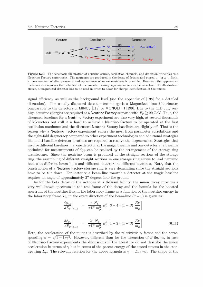
6.6 Neutrino Factories 59

Source Oscillation Detection

ΠK

ΝΜ

Μ-

Ν

e

ΝΜ

Νe

Ν

eΝ

Μ

Μ-

e-

e+

Μ+

CC

CC

CC

CC

Θ23 , ÈDm312È

Θ13 , ∆CP

50%

50%

99%

Figure 6.5: The schematic illustration of neutrino source, oscillation channels, and detection principles at aNeutrino Factory experiment. The neutrinos are produced in the decay of boosted and stored µ− or µ+. Both,a measurement of disappearance and appearance of muon neutrinos is possible. However, the appearancemeasurement involves the detection of the so-called wrong sign muons as can be seen from the illustration.Hence, a magnetized detector has to be used in order to allow for charge identification of the muons.

signal efficiency as well as the background level (see the appendix of [198] for a detaileddiscussion). The usually discussed detector technology is a Magnetized Iron Calorimetercomparable to the detectors of MINOS [119] or MONOLITH [199]. Due to the CID cut, veryhigh neutrino energies are required at a Neutrino Factory scenario with Eν & 20 GeV. Thus, thediscussed baselines for a Neutrino Factory experiment are also very high, at several thousandsof kilometers but still it is hard to achieve a Neutrino Factory to be operated at the firstoscillation maximum and the discussed Neutrino Factory baselines are slightly off. That is thereason why a Neutrino Factory experiment suffers the most from parameter correlations andthe eight-fold degeneracy compared to other experiment technologies and additional strategieslike multi-baseline detector locations are required to resolve the degeneracies. Strategies thatinvolve different baselines, i.e. one detector at the magic baseline and one detector at a baselineoptimized for measurements of δCP can be realized by the arrangement of the storage ringarchitecture. Since the neutrino beam is produced at the straight sections of the storagering, the assembling of different straight sections in one storage ring allows to lead neutrinobeams to different beam lines and different detectors at different baselines. Note, that theconstruction of a Neutrino Factory storage ring is very demanding since the straight sectionshave to be tilt down. For instance a beam-line towards a detector at the magic baselinerequires an angle of approximately 37 degrees into the ground.

As for the beta decay of the isotopes at a β-Beam facility, the muon decay provides avery well-known spectrum in the rest frame of the decay and the formula for the boostedspectrum of the neutrino flux in the laboratory frame as a function of the neutrino energy inthe laboratory frame Eν in the exact direction of the beam-line (θ = 0) is given as:

dφνµ

dEν

∣∣∣∣θ=0

=4 Nµ

πL2 m3µ

E2ν

[

3 − 4 γ(1 − β)Eν

mµ

]

dφνe

dEν

∣∣∣∣θ=0

=24 Nµ

πL2 m3µ

E2ν

[

1 − 2 γ(1 − β)Eν

mµ

]

(6.11)

Here, the acceleration of the muons is described by the relativistic γ factor and the corre-sponding β =

√

1 − 1/γ2. However, different than for the discussion of β-Beams, in caseof Neutrino Factory experiments the discussions in the literature do not describe the muonacceleration in terms of γ but in terms of the parent energy of the stored muons in the stor-age ring Eµ. The relevant relation for the above formula is γ = Eµ/mµ. The shape of the

60 CHAPTER 6. Long Baseline Experiment Scenarios

EΝ

Neu

trin

oF

lux

Neutrino Factory Flux

Νe Ν

e

Ν

Μ ΝΜ

Figure 6.6: The energy spectrum of the neutrino flux at a Neutrino Factory experiment. The neutrino fluxconsists either of νµ and νe for stored µ− or νµ and νe for stored µ+. The maximal energy is Emax = Eµ, theenergy of the parent muons in the storage ring.

neutrino flux at a Neutrino Factory is illustrated in Fig. 6.6. The electron neutrino and muonneutrino contributions follow different behaviors and the maximal flux for electron neutrinosis obtained at neutrino energies smaller than Eµ while the maximal muon neutrino flux isobtained at the highest possible energy, the initial energy of the stored parent muon Eµ.

The technology of conventional beam production and beam production at a NeutrinoFactory is not as disconnected as it may seem, because the muons for the decay in the storagerings are to be produced in the decay of pions just as the neutrinos in conventional beamproduction. The storage selection of either muons or anti-muons is performed by the selectionof the π+ or π− at the target by the polarization of the magnetized horns. The main challengefor the further handling of the produced muons in the decays of the pions is the issue of muoncooling. The initially produced muons have a wide distribution in momentum space but arerequired to be cooled down to allow for a further clean acceleration [193,200–204]. The mostpromising technology for the required muon cooling is the so-called ionization cooling [205,206]since all existing cooling technologies do not work for muons. The feasibility of this technologyis to be proved at the MICE experiment [207–209]. It should be mentioned that a successfultechnology for the muon cooling is not only required for neutrino oscillation physics at aNeutrino Factory but is also a very important issue for the feasibility of a possible future muoncollider experiment [210,211].

It should be noted, that a Neutrino Factory experiment is not only a very good tool forstandard three-flavor oscillations but is also sensitive to possible deviations from the“standardphysics”and “new physics”would be observable, as for instance the possibility of the so-callednon-standard interactions of neutrinos that mediate additional flavor transition contributionsand interfere with the oscillation. These have been addressed in [212–219]. Since we willnot implement non-standard interactions to the simulations in this work, it should be keptin mind that the optimization arguments discussed in this work do not correspond to the

6.6 Neutrino Factories 61

optimization with respect to all physical motivations but only to the standard three-flavoroscillation.

62 CHAPTER 6. Long Baseline Experiment Scenarios

63

Chapter 7

Beta Beam Performance

The aim for this Chapter is to estimate and optimize the performance of a possible β-Beamexperiment for measurements of sin2 2θ13, the phase δCP, and the sign of ∆m2

31. First, weintroduce the simulation methods that have been used to analyze the physics potential ofthe β-Beam. Next, the possible optimization in terms of neutrino energy, i.e. the isotopeacceleration factor γ, and the experiment baseline L are addressed. Thereafter single technicalaspects and possible impacts on the physics potential are discussed, before optimized referencescenarios with different ambitious detector effort and technology are defined and the potentialis compared. Furthermore, the performance of these reference setups is related to optimizedNeutrino Factory reference scenarios in Chapter 9.

7.1 Beta Beam Simulation

All β-Beam simulations throughout this work are performed with the GLoBES software [220,221] that is briefly introduced in the appendix. For all discussed β-Beam scenarios we assumea total runtime of 8 years data taking. The endpoint of the spectrum of the neutrino fluxis determined by the tuned γ acceleration factor and the endpoint energy E0 of the usedisotopes, here 18Ne (νe-beam) and 6He with endpoint energies E0 = 3.4 MeV for 18Ne andE0 = 3.5 MeV for 6He. The endpoint energies of the two nuclei are very similar and weassume the same acceleration factors for both, i.e. γ(18Ne) = γ(6He), so that the neutrinoenergies in the anti-neutrino and neutrino modes are very similar. In principle, the γ’s can bechosen differently, however there is no obvious gain in increasing one with respect to the other(cf., Ref. [180]). We neglect the fact that there exist different excited states in the daughternuclei of the decay, which additionally lead to negligible small contributions to the spectrawith different endpoint energies. We assume 2.9 · 10−18 6He and 1.1 · 10−18 18Ne isotopedecays per year in the storage rings. This assumes a concurrent neutrino and anti-neutrinoruntime with both isotopes operated over the absolute runtime of 8 years and correspondsto the standard assumption for β-Beams in the literature [176–187] . The same statistics canalso be obtained by a consecutive neutrino and anti-neutrino runtime of 4 years each withthe double numbers of the decays per year. However, these numbers are based on estimatesfor low γ with the acceleration factors γ(18Ne) = 100 and γ(6He) = 60 and it has not beendemonstrated that the numbers of decays can be maintained for medium or high γ. Basically,we assume that this is the case but the impact of a γ-scaling of the isotope decays is addressedin Section 7.5 since the assumption might not be justified for technical considerations.

64 CHAPTER 7. Beta Beam Performance

An important difference of a β-Beam experiment to Superbeams or Neutrino Factory ex-periments is the missing information on the leading atmospheric oscillation parameters inthe disappearance data. In principle ∆m2

31 is accessible while sin2 2θ23 is not, however thiswould require systematical uncertainties below the 1% level which is hardly achievable. So, aβ-Beam experiment itself cannot measure the leading parameters and is not able to contributeto the desirable precision measurements of the atmospheric parameters as would be the casefor Superbeams or a Neutrino Factory. Here, we are mainly interested in the performance ofthe appearance measurements to determine sin2 2θ13, δCP, and the neutrino mass hierarchy.But as was pointed out earlier, the leading parameters also affect this performance via param-eter correlations. So, we add the simulated disappearance data of the Superbeam experimentT2K1 (8 years assumed) to minimize the parameter correlations with the leading atmosphericoscillation parameters. At the time a β-Beam starts operation this data will be available toconstrain the parameters. However, we do not include the T2K appearance data in order toanalyze the performance of the β-Beam appearance measurements alone. The impact of theinclusion of the T2K disappearance data is addressed in Section 7.4. We will apply the sametechnique in the simulations of the Neutrino Factory experiments and for the simulation ofT2HK since these experiments will have the ability to measure the atmospheric parametersby far best from their own disappearance data that is included to the simulation.

The solar oscillation parameters are constrained with a precision of 5% for each indepen-dently to the best-fit values by GLoBES internal priors with pull terms in the χ2 calculation.Eventually, we assume a constant matter density profile with a 5 % uncertainty on the valueof the baseline-averaged matter density, where the uncertainty takes into account matterdensity uncertainties as well as matter density profile effects [224–226]. If the baseline ofan experiment is changed, we also re-compute and use the average matter density for thisbaseline.

Detector technologies

A general requirement for any β-Beam detector is to have good muon-electron separationcapabilities and to have an efficient neutral-current rejection. At the same time, the technologymust be available and cost effective to allow in time a scaling to large detectors. For lowervalues of γ, certainly Water Cherenkov detectors fulfill these criteria [175, 176, 179, 180, 182,183]. However, at higher γ values, the lack of background discrimination in Water Cherenkovdetectors becomes a huge problem and other detector types, such as calorimeters or TPCs(Time Projection Chambers) are more suitable [179, 227]. The precise value of γ where thisturnover happens seems to be an unresolved question and different views can be found in theliterature [176,179]. Our choice for large values of γ is the so-called Totally Active Scintillatordetector for reasons which will be discussed below. The two detector technologies used in thisstudy, namely Water Cherenkov and Totally Active Scintillator, are described in more detailin the following subsections.

Water Cherenkov Detector

Water Cherenkov detectors are well suited to distinguish muon neutrinos from electron neutri-nos by analyzing the topology of the detected Cherenkov ring. However, background rejection

1See Refs. [198,222,223] for details of the T2K description within GLoBES. The corresponding experimentdescribing file is provided with the GLoBES 3.0 software. The here used file is a modified version of T2K.glb.

7.1 Beta Beam Simulation 65

can be a problem in using a Water Cherenkov detector in combination with a β-Beam. Themain source of background to the muon neutrino appearance search will be the flavor-blindneutral-current events which are mistaken for muon neutrino charged-current events. Themost critical neutral-current events are those where one or several energetic pions are in-volved, which implies that there is basically no background below the pion production thresh-old around 200MeV. Therefore, one solution would be to tune γ to a low value where most ofthe neutrinos in the beam are below this threshold [176]. In that case there would be no en-ergy information, since the Fermi-motion of the nucleons would induce an energy smearing ofabout 100MeV. This would reduce the β-Beam to a mere counting experiment, which wouldhave only a very limited physics reach [179]. Above the pion threshold, the feasibility of usinga Water Cherenkov detector depends on the ability to correctly identify pions and to rejectneutral-current events. The pion identification works, in principle, by identifying its decayprocess and it seems to be possible up to some level. There are very different statements inthe literature how well this can be done [176,179]. The different results can to a large extentbe attributed to the different level of detail used in the detector simulation.

In order to describe the energy response of the detector in our study, we divide thesignal events into samples of quasi-elastic events (QE) and inelastic events (IE). Only forthe QE sample, it is possible to accurately reconstruct the neutrino energy from the chargedlepton. For IE events, the reconstructed energy will always lie below the true (incident)neutrino energy because the hadronic component of the interaction cannot be seen by aWater Cherenkov detector. Since the separation of those two event samples is fraud with alarge error, we will use the same technique as described in Ref. [198]. This means that thetotal rates number of all IE + QE events is taken into account and in addition the spectrumof the QE event sample is used to obtain spectral information. In order to avoid doublecounting of events, the QE event sample is taken only with a free normalization. In thisapproach, no particular assumption about the event by event separation has to be made,because this approach is purely statistical. In fact, the real experiment might even performbetter since there actually could be some event by event separation. For the spectral analysis,we assume that the Fermi-motion is the main component of the resulting energy resolutionfunction. Therefore, a constant width of 85MeV [146] in a Gaußian energy resolution functionis taken, in order to describe the energy reconstruction of the QE sample. For the backgrounddistribution, we make the assumption that every neutrino which interacts via neutral-currentsis reconstructed with an energy distribution which is flat from zero up to the true neutrinoenergy. In this way we obtain a background which is peaked at low energies. We do not takeinto account any other background source, since in Ref. [180] it was shown that atmosphericneutrinos only give a very small contribution.

In order to be able to use γ values in the range from 50 to 500, the energy range is chosenas 0.2−3.0GeV and is divided into bins of 100MeV width, such that the total number of binsis 28. All efficiencies are constant with exception of the first bin where they are only 1/2 ofthe value given in the signal/background table to account for threshold effects. The numbersfor the disappearance channel could be quite different (in fact, the efficiencies might be muchhigher), but we checked that the final results do not depend on this assumption. Therefore,because of simplicity, we take the same numbers as for the appearance channels. We also in-clude systematic uncertainties on the normalization of signal and background events as givenin Table 7.1, where all errors are assumed to be fully uncorrelated. This is a conservativeapproximation and does not affect the result from the appearance measurement. The disap-pearance measurement, on the other hand, would require a total absolute error of less than

66 CHAPTER 7. Beta Beam Performance

Disappearance – 18Ne stored σnorm σcal

Signal 0.55 ⊗ (νe → νe)QE 0.025 10−4

Background 0.003 ⊗ (νe → νx)NC 0.05 10−4

Appearance – 18Ne stored – Spectrum

Signal 0.55 ⊗ (νe → νµ)QE 10.0 10−4

Background 0.003 ⊗ (νe → νx)NC 0.05 10−4

Appearance – 18Ne stored – Total Rates

Signal 0.55 ⊗ (νe → νµ)CC 0.025 10−4

Background 0.003 ⊗ (νe → νx)NC 0.05 10−4

Disappearance – 6He stored

Signal 0.75 ⊗ (νe → νe)QE 0.025 10−4

Background 0.0025 ⊗ (νe → νx)NC 0.05 10−4

Appearance – 6He stored – Spectrum

Signal 0.75 ⊗ (νe → νµ)QE 10.0 10−4

Background 0.0025 ⊗ (νe → νx)NC 0.05 10−4

Appearance – 6He stored – Total Rates

Signal 0.75 ⊗ (νe → νµ)CC 0.025 10−4

Background 0.0025 ⊗ (νe → νx)NC 0.05 10−4

Table 7.1: The signal efficiencies and background rejection factors together with the associated systematicalerrors for the various signals and backgrounds used in our description of the performance of a Water Cherenkovdetector β-Beam. The normalization errors are the normalization error σnorm and the energy calibration errorσcal. This corresponds to the BBvar_WC.glb file that is provided with GLOBES 3.0.

1% to yield any information on θ13 [155,228,229]. This number, however, seems very difficultto be reached, if at all, for any experiment which involves neutrino-nucleus cross-sections atlow energies. Our parameterization has been calibrated against low γ scenarios from earlierliterature (γ = 150, [180]). Therefore using different values of γ involves some extrapolation.Our parameterization should nevertheless be reliable from γ 100 up to 350, and it shouldadditionally reproduce the qualitative features of the γ-scaling within a range from 50 to 500.The experiment description is similar to the one from [186] and is provided with the newestversion of GLoBES 3.0 [220,221].

Totally Active Scintillator Detector

For even larger values of γ, a detector which can also measures the hadronic energy depositionis required. The reason is that the fraction of inelastic events in the whole event sampleincreases with increasing γ, because the neutrino spectra are extended to higher energies.The techniques which have traditionally been used for that purpose are tracking calorimetersand TPCs (such as a large liquid Argon TPC as described in Ref. [227]). The latter technologyhas certainly a great potential in neutrino physics, but given the fact that background issuesare not the primary concern, we will discuss the more traditional and better understood optionof a tracking calorimeter. Basically, there exist three different approaches:

• magnetized iron plates, interleaved with scintillator bars

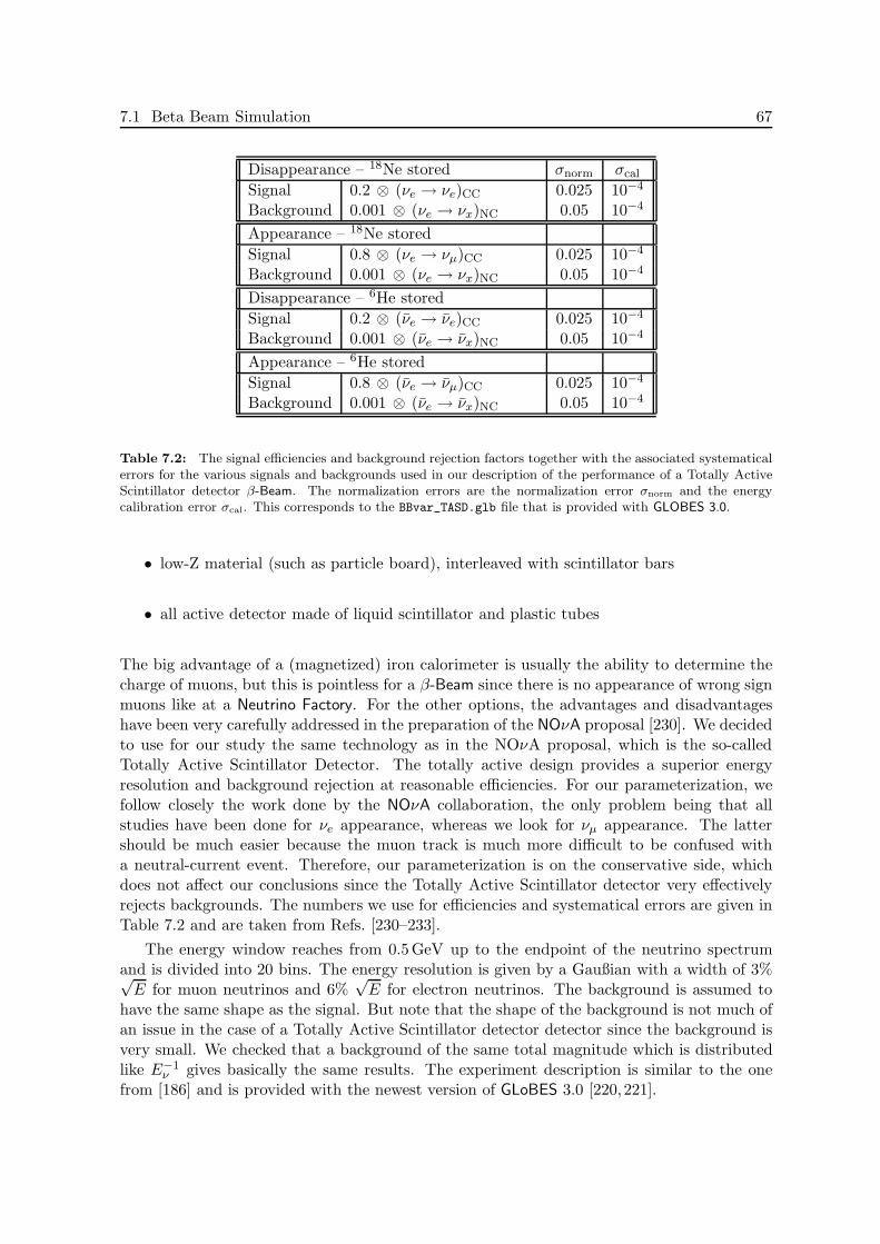
7.1 Beta Beam Simulation 67

Disappearance – 18Ne stored σnorm σcal

Signal 0.2 ⊗ (νe → νe)CC 0.025 10−4

Background 0.001 ⊗ (νe → νx)NC 0.05 10−4

Appearance – 18Ne stored

Signal 0.8 ⊗ (νe → νµ)CC 0.025 10−4

Background 0.001 ⊗ (νe → νx)NC 0.05 10−4

Disappearance – 6He stored

Signal 0.2 ⊗ (νe → νe)CC 0.025 10−4

Background 0.001 ⊗ (νe → νx)NC 0.05 10−4

Appearance – 6He stored

Signal 0.8 ⊗ (νe → νµ)CC 0.025 10−4

Background 0.001 ⊗ (νe → νx)NC 0.05 10−4

Table 7.2: The signal efficiencies and background rejection factors together with the associated systematicalerrors for the various signals and backgrounds used in our description of the performance of a Totally ActiveScintillator detector β-Beam. The normalization errors are the normalization error σnorm and the energycalibration error σcal. This corresponds to the BBvar_TASD.glb file that is provided with GLOBES 3.0.

• low-Z material (such as particle board), interleaved with scintillator bars

• all active detector made of liquid scintillator and plastic tubes

The big advantage of a (magnetized) iron calorimeter is usually the ability to determine thecharge of muons, but this is pointless for a β-Beam since there is no appearance of wrong signmuons like at a Neutrino Factory. For the other options, the advantages and disadvantageshave been very carefully addressed in the preparation of the NOνA proposal [230]. We decidedto use for our study the same technology as in the NOνA proposal, which is the so-calledTotally Active Scintillator Detector. The totally active design provides a superior energyresolution and background rejection at reasonable efficiencies. For our parameterization, wefollow closely the work done by the NOνA collaboration, the only problem being that allstudies have been done for νe appearance, whereas we look for νµ appearance. The lattershould be much easier because the muon track is much more difficult to be confused witha neutral-current event. Therefore, our parameterization is on the conservative side, whichdoes not affect our conclusions since the Totally Active Scintillator detector very effectivelyrejects backgrounds. The numbers we use for efficiencies and systematical errors are given inTable 7.2 and are taken from Refs. [230–233].

The energy window reaches from 0.5GeV up to the endpoint of the neutrino spectrumand is divided into 20 bins. The energy resolution is given by a Gaußian with a width of 3%√

E for muon neutrinos and 6%√

E for electron neutrinos. The background is assumed tohave the same shape as the signal. But note that the shape of the background is not much ofan issue in the case of a Totally Active Scintillator detector detector since the background isvery small. We checked that a background of the same total magnitude which is distributedlike E−1

ν gives basically the same results. The experiment description is similar to the onefrom [186] and is provided with the newest version of GLoBES 3.0 [220,221].

68 CHAPTER 7. Beta Beam Performance

7.2 Beta Beam Optimization

In this section, we will focus on the optimization of a β-Beam experiment in terms of opti-mizing the baseline L or the neutrino energy Eν by tuning the isotope acceleration γ. Suchan optimization attempt was already performed in [186] for a slightly different set of trueoscillation parameter values. There, the optimization process involved a tuning of γ by fixingthe ratio L/γ so that higher γ also implies a larger baseline. As outcome for both scenarios,Water Cherenkov and Totally Active Scintillator, the simple rule “the larger γ, the better”was found, however slightly more effective for the latter. We will not repeat this discussionand focus on the single optimization of either baseline L for a selected fixed γ or the isotopeacceleration γ for a selected fixed baseline L. We will discuss the optimization for the threeperformance indicators: sensitivity limit to sin2 2θ13, sensitivity to maximal CP violation, andsensitivity to mass hierarchy. These performance indicators will be shortly described whenfirst discussed, however a list of all performance indicators together with the exact definitionand further useful comments is given in the appendix. The performance indicators will beintroduced to describe the abilities of the considered experiment scenarios in measurementsof sin2 2θ13, δCP, and the mass hierarchy2.

For the discussion of the optimization issues concerning the baseline L we discuss a low γβ-Beam with a Water Cherenkov (γ = 150), two medium γ β-Beams, one Water Cherenkov(γ = 350) and one Totally Active Scintillator detector scenario (γ = 500), and finally ahigh γ scenario with a Totally Active Scintillator detector (γ = 1000). For the discussion ofthe optimization issues concerning the isotope acceleration factor γ we try to stick to realisticbaselines. For that reason a Water Cherenkov β-Beam is discussed at the CERN-Frejus baselineof L=130 km. So, the CERN-MEMPHYS baseline scenario is included [187, 234]. A secondbaseline is discussed for a Water Cherenkov detector at a distance of L=730 km. This baselinecan be associated with the distance between the CERN and the Gran Sasso undergroundlaboratories in Italy or to the baseline between the FermiLab and the Soudan mine, i.e. theactual MINOS baseline. This baseline is large enough for β-Beam energies where already aTotally Active Scintillator detector can be installed so we will also discuss this possibility andadditionally also a Totally Active Scintillator detector scenario at an even larger baseline ofL=1500 km.

Sensitivity to θ13

The sensitivity limit to sin2 2θ13 describes the ability of an experiment to set a lower boundto sin2 2θ13 in the worst-case scenario3 of a vanishing true value sin2 2θ13 = 0. It is given bythe largest fit value of sin2 2θ13 that can be excluded at the chosen confidence level, that ishere and throughout this work 3σ, under the simulation assumption sin2 2θtrue

13 = 0.First, we concentrate on the optimization of the baseline for a low γ = 150 and a medium

γ = 350 β-Beam with a megaton Water Cherenkov detector. The respective sensitivity limitsto sin2 2θ13 as a function of the baseline L are shown in Fig. 7.1. In order to allow comparisonof the results with results from the corresponding discussion in [186] the upper x-axis is labeled

2For reasons of intuitive lucidity a color coding has been introduced to the screen version and selected printversions in the chapters where the main results are presented, that is each parameter corresponds to its owncolor. All performance indicators involving sin2 2θ13 are indicated with blue colors, the ones involving δCP areshown in red colors, and the sensitivity to mass hierarchy is always associated with green colors.

3Here, the term worst-case scenario is used from a view point of the experiment, since sin2 2θ13 = 0 wouldeffect in a non-observation of three-flavor effects at the experiment.

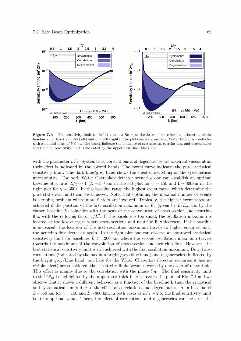
7.2 Beta Beam Optimization 69

100 200 300 400 500 600L @kmD

10-4

10-3

10-2

10-1

Sen

sitiv

itylim

itto

sin2

2Θ13

0.5 1 1.5 2 2.5 3 3.5 4LΓ

BB - Γ=150 - WC

3Σ

GLoBES 3.0 H2007L

Systematics

Correlations

Degeneracies

100 200 300 400 500 600L @kmD

10-4

10-3

10-2

10-1

Sen

sitiv

itylim

itto

sin2

2Θ13

0.5 1 1.5 2 2.5 3 3.5 4LΓ

250 500 750 1000 1250 1500L @kmD

10-4

10-3

10-2

10-1

Sen

sitiv

itylim

itto

sin2

2Θ13

0.5 1 1.5 2 2.5 3 3.5 4LΓ

BB - Γ=350 - WC

3Σ

GLoBES 3.0 H2007L

Systematics

Correlations

Degeneracies

250 500 750 1000 1250 1500L @kmD

10-4

10-3

10-2

10-1

Sen

sitiv

itylim

itto

sin2

2Θ13

0.5 1 1.5 2 2.5 3 3.5 4LΓ

Figure 7.1: The sensitivity limit to sin2 2θ13 at a β-Beam at the 3σ confidence level as a function of thebaseline L for fixed γ = 150 (left) and γ = 350 (right). The plots are for a megaton Water Cherenkov detectorwith a fiducial mass of 500 kt. The bands indicate the influence of systematics, correlations, and degeneraciesand the final sensitivity limit is indicated by the uppermost thick black line.

with the parameter L/γ. Systematics, correlations and degeneracies are taken into account antheir effect is indicated by the colored bands. The lowest curve indicates the pure statisticalsensitivity limit. The dark blue/grey band shows the effect of switching on the systematicaluncertainties. For both Water Cherenkov detector scenarios one can establish an optimalbaseline at a ratio L/γ ∼ 1 (L ∼150 km in the left plot for γ = 150 and L∼ 300km in theright plot for γ = 350). In this baseline range the highest event rates (which determine thepure statistical limit) can be achieved. Note, that obtaining the maximal number of eventsis a tuning problem where more factors are involved. Typically, the highest event rates areachieved if the position of the first oscillation maximum in Eν (given by L/Eν , i.e. by thechosen baseline L) coincides with the peak of the convolution of cross section and neutrinoflux with the reducing factor 1/L2. If the baseline is too small, the oscillation maximum islocated at too low energies where cross sections and neutrino flux decrease. If the baselineis increased, the location of the first oscillation maximum travels to higher energies, untilthe neutrino flux decreases again. In the right plot one can observe an improved statisticalsensitivity limit for baselines L > 1200 km where the second oscillation maximum travelstowards the maximum of the convolution of cross section and neutrino flux. However, thebest statistical sensitivity limit is still achieved with the first oscillation maximum. But, if alsocorrelations (indicated by the medium bright grey/blue band) and degeneracies (indicated bythe bright grey/blue band, but here for the Water Cherenkov detector scenarios it has novisible effect) are considered, the sensitivity limit becomes worse by one order of magnitude.This effect is mainly due to the correlation with the phase δCP. The final sensitivity limitto sin2 2θ13 is highlighted by the uppermost thick black curve in the plots of Fig. 7.1 and weobserve that it shows a different behavior as a function of the baseline L than the statisticaland systematical limits due to the effect of correlations and degeneracies. At a baseline ofL ∼350 km for γ = 150 and L ∼800 km, in both cases at L/γ ∼ 2.5, the final sensitivity limitis at its optimal value. There, the effect of correlations and degeneracies vanishes, i.e. the

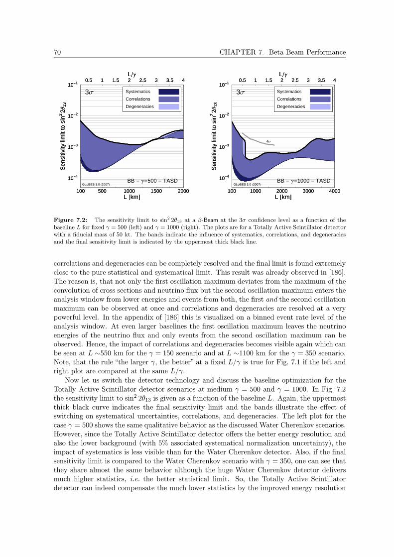
70 CHAPTER 7. Beta Beam Performance

100 500 1000 1500 2000L @kmD

10-4

10-3

10-2

10-1

Sen

sitiv

itylim

itto

sin2

2Θ13

0.5 1 1.5 2 2.5 3 3.5 4LΓ

BB - Γ=500 - TASD

3Σ

GLoBES 3.0 H2007L

Systematics

Correlations

Degeneracies

100 500 1000 1500 2000L @kmD

10-4

10-3

10-2

10-1

Sen

sitiv

itylim

itto

sin2

2Θ13

0.5 1 1.5 2 2.5 3 3.5 4LΓ

100 1000 2000 3000 4000L @kmD

10-4

10-3

10-2

10-1

Sen

sitiv

itylim

itto

sin2

2Θ13

0.5 1 1.5 2 2.5 3 3.5 4LΓ

BB - Γ=1000 - TASD

3Σ

GLoBES 3.0 H2007L

Systematics

Correlations

Degeneracies

4Σ

100 1000 2000 3000 4000L @kmD

10-4

10-3

10-2

10-1

Sen

sitiv

itylim

itto

sin2

2Θ13

0.5 1 1.5 2 2.5 3 3.5 4LΓ

Figure 7.2: The sensitivity limit to sin2 2θ13 at a β-Beam at the 3σ confidence level as a function of thebaseline L for fixed γ = 500 (left) and γ = 1000 (right). The plots are for a Totally Active Scintillator detectorwith a fiducial mass of 50 kt. The bands indicate the influence of systematics, correlations, and degeneraciesand the final sensitivity limit is indicated by the uppermost thick black line.

correlations and degeneracies can be completely resolved and the final limit is found extremelyclose to the pure statistical and systematical limit. This result was already observed in [186].The reason is, that not only the first oscillation maximum deviates from the maximum of theconvolution of cross sections and neutrino flux but the second oscillation maximum enters theanalysis window from lower energies and events from both, the first and the second oscillationmaximum can be observed at once and correlations and degeneracies are resolved at a verypowerful level. In the appendix of [186] this is visualized on a binned event rate level of theanalysis window. At even larger baselines the first oscillation maximum leaves the neutrinoenergies of the neutrino flux and only events from the second oscillation maximum can beobserved. Hence, the impact of correlations and degeneracies becomes visible again which canbe seen at L ∼550 km for the γ = 150 scenario and at L ∼1100 km for the γ = 350 scenario.Note, that the rule “the larger γ, the better” at a fixed L/γ is true for Fig. 7.1 if the left andright plot are compared at the same L/γ.

Now let us switch the detector technology and discuss the baseline optimization for theTotally Active Scintillator detector scenarios at medium γ = 500 and γ = 1000. In Fig. 7.2the sensitivity limit to sin2 2θ13 is given as a function of the baseline L. Again, the uppermostthick black curve indicates the final sensitivity limit and the bands illustrate the effect ofswitching on systematical uncertainties, correlations, and degeneracies. The left plot for thecase γ = 500 shows the same qualitative behavior as the discussed Water Cherenkov scenarios.However, since the Totally Active Scintillator detector offers the better energy resolution andalso the lower background (with 5% associated systematical normalization uncertainty), theimpact of systematics is less visible than for the Water Cherenkov detector. Also, if the finalsensitivity limit is compared to the Water Cherenkov scenario with γ = 350, one can see thatthey share almost the same behavior although the huge Water Cherenkov detector deliversmuch higher statistics, i.e. the better statistical limit. So, the Totally Active Scintillatordetector can indeed compensate the much lower statistics by the improved energy resolution

7.2 Beta Beam Optimization 71

100 200 300 400 500Γ

10-4

10-3

10-2

10-1

Sen

sitiv

itylim

itto

sin2

2Θ13

2 1 0.5 0.3LΓ

BB - L=130km - WC

3Σ

GLoBES 3.0 H2007L

Systematics

Correlations

Degeneracies

100 200 300 400 500Γ

10-4

10-3

10-2

10-1

Sen

sitiv

itylim

itto

sin2

2Θ13

2 1 0.5 0.3LΓ

200 300 400 500Γ

10-4

10-3

10-2

10-1

Sen

sitiv

itylim

itto

sin2

2Θ13

4 3 2.5 2 1.5LΓ

BB - L=730km - WC

3Σ

GLoBES 3.0 H2007L

Systematics

Correlations

Degeneracies

200 300 400 500Γ

10-4

10-3

10-2

10-1

Sen

sitiv

itylim

itto

sin2

2Θ13

4 3 2.5 2 1.5LΓ

Figure 7.3: The sensitivity limit to sin2 2θ13 at a β-Beam at the 3σ confidence level as a function of γ forthe fixed baselines L = 130 km (left) and L = 730 km (right). The plots are for a Water Cerenkov detectorwith a fiducial mass of 500 kt. The bands indicate the influence of systematics, correlations, and degeneraciesand the final sensitivity limit is indicated by the uppermost thick black line.

and signal/background ratio when it comes to resolving the correlations and degeneracies.

By regarding the right plot of Fig. 7.2, a slightly different behavior of the sensitivitylimit can be observed. First, the correlations and degeneracies have a remaining effect atbaselines, where events from both, the first and second oscillation maximum can be observed.However, still the effect is much smaller than for other baselines and the combination offirst and second oscillation maximum helps in resolving the correlations and degeneracies.The second visual difference is the behavior at the first oscillation maximum at L ∼800 kmwhere now the optimal final sensitivity limit can be obtained due to a jump by half an orderof magnitude at L ∼600 km. This behavior is well known from the simulation of NeutrinoFactory experiments and will also occur in the next chapter when these are discussed. Theeffect arises from the phenomenology of the (θ13, δCP-degeneracy) that appears at larger fitvalues of sin2 2θ13 as a local minimum in the χ2-distribution while the global minimum islocated at the true value sin2 2θ13 = 0. For two example scenarios, this local degenerateminimum in the χ2-distribution can be nearly identical but once slightly above and onceslightly below the chosen confidence level, i.e. it can or cannot be excluded at that confidencelevel. Consequently the two example scenarios, although almost identical in the performance,would be attributed with quite different sin2 2θ13 sensitivity limits separated by half ormore of an order of magnitude. Thus, the visible jump at L ∼600 km in the right plotof Fig. 7.2 has to be treated very carefully when it comes to interpretation. In order toillustrate this effect, the sensitivity limit at the 4σ confidence level is also indicated in theplot by the thick grey line between 500 km. L .2000 km. It is obvious, that the hugeimprovement of the final limit at the 3σ level is not robust and vanishes already at 4σ.Hence, the interpretation has to be, that the true performance of the γ = 1000 scenario doesindeed not change so dramatically in that range as could be naively deduced from the 3σ curve.

As already mentioned, not only the baseline can be optimized at a β-Beam experiment but

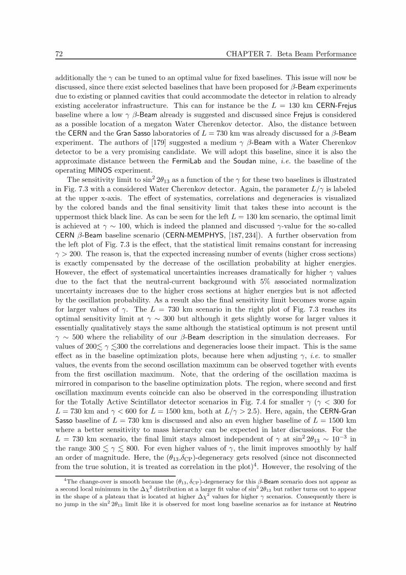
72 CHAPTER 7. Beta Beam Performance

additionally the γ can be tuned to an optimal value for fixed baselines. This issue will now bediscussed, since there exist selected baselines that have been proposed for β-Beam experimentsdue to existing or planned cavities that could accommodate the detector in relation to alreadyexisting accelerator infrastructure. This can for instance be the L = 130 km CERN-Frejusbaseline where a low γ β-Beam already is suggested and discussed since Frejus is consideredas a possible location of a megaton Water Cherenkov detector. Also, the distance betweenthe CERN and the Gran Sasso laboratories of L = 730 km was already discussed for a β-Beamexperiment. The authors of [179] suggested a medium γ β-Beam with a Water Cherenkovdetector to be a very promising candidate. We will adopt this baseline, since it is also theapproximate distance between the FermiLab and the Soudan mine, i.e. the baseline of theoperating MINOS experiment.

The sensitivity limit to sin2 2θ13 as a function of the γ for these two baselines is illustratedin Fig. 7.3 with a considered Water Cherenkov detector. Again, the parameter L/γ is labeledat the upper x-axis. The effect of systematics, correlations and degeneracies is visualizedby the colored bands and the final sensitivity limit that takes these into account is theuppermost thick black line. As can be seen for the left L = 130 km scenario, the optimal limitis achieved at γ ∼ 100, which is indeed the planned and discussed γ-value for the so-calledCERN β-Beam baseline scenario (CERN-MEMPHYS, [187, 234]). A further observation fromthe left plot of Fig. 7.3 is the effect, that the statistical limit remains constant for increasingγ > 200. The reason is, that the expected increasing number of events (higher cross sections)is exactly compensated by the decrease of the oscillation probability at higher energies.However, the effect of systematical uncertainties increases dramatically for higher γ valuesdue to the fact that the neutral-current background with 5% associated normalizationuncertainty increases due to the higher cross sections at higher energies but is not affectedby the oscillation probability. As a result also the final sensitivity limit becomes worse againfor larger values of γ. The L = 730 km scenario in the right plot of Fig. 7.3 reaches itsoptimal sensitivity limit at γ ∼ 300 but although it gets slightly worse for larger values itessentially qualitatively stays the same although the statistical optimum is not present untilγ ∼ 500 where the reliability of our β-Beam description in the simulation decreases. Forvalues of 200. γ .300 the correlations and degeneracies loose their impact. This is the sameeffect as in the baseline optimization plots, because here when adjusting γ, i.e. to smallervalues, the events from the second oscillation maximum can be observed together with eventsfrom the first oscillation maximum. Note, that the ordering of the oscillation maxima ismirrored in comparison to the baseline optimization plots. The region, where second and firstoscillation maximum events coincide can also be observed in the corresponding illustrationfor the Totally Active Scintillator detector scenarios in Fig. 7.4 for smaller γ (γ < 300 forL = 730 km and γ < 600 for L = 1500 km, both at L/γ > 2.5). Here, again, the CERN-GranSasso baseline of L = 730 km is discussed and also an even higher baseline of L = 1500 kmwhere a better sensitivity to mass hierarchy can be expected in later discussions. For theL = 730 km scenario, the final limit stays almost independent of γ at sin2 2θ13 ∼ 10−3 inthe range 300 . γ . 800. For even higher values of γ, the limit improves smoothly by halfan order of magnitude. Here, the (θ13,δCP)-degeneracy gets resolved (since not disconnectedfrom the true solution, it is treated as correlation in the plot)4. However, the resolving of the

4The change-over is smooth because the (θ13, δCP)-degeneracy for this β-Beam scenario does not appear asa second local minimum in the ∆χ2 distribution at a larger fit value of sin2 2θ13 but rather turns out to appearin the shape of a plateau that is located at higher ∆χ2 values for higher γ scenarios. Consequently there isno jump in the sin2 2θ13 limit like it is observed for most long baseline scenarios as for instance at Neutrino

7.2 Beta Beam Optimization 73

200 400 600 800 1000Γ

10-4

10-3

10-2

10-1

Sen

sitiv

itylim

itto

sin2

2Θ13

3 2 1.5 1 0.8LΓ

BB - L=730km - TASD

3Σ

GLoBES 3.0 H2007L

Systematics

Correlations

Degeneracies

4Σ

200 400 600 800 1000Γ

10-4

10-3

10-2

10-1

Sen

sitiv

itylim

itto

sin2

2Θ13

3 2 1.5 1 0.8LΓ

400 500 600 700 800 900 1000Γ

10-4

10-3

10-2

10-1

Sen

sitiv

itylim

itto

sin2

2Θ13

3 2.5 2 1.5LΓ

BB - L=1500km - TASD

3Σ

GLoBES 3.0 H2007L

Systematics

Correlations

Degeneracies

400 500 600 700 800 900 1000Γ

10-4

10-3

10-2

10-1

Sen

sitiv

itylim

itto

sin2

2Θ13

3 2.5 2 1.5LΓ

Figure 7.4: The sensitivity limit to sin2 2θ13 at a β-Beam at the 3σ confidence level as a function of γ forthe fixed baselines L = 730 km (left) and L = 1500 km (right). The plots are for a Totally Active Scintillatordetector with a fiducial mass of 50 kt. The bands indicate the influence of systematics, correlations, anddegeneracies and the final sensitivity limit is indicated by the uppermost thick black line.

(θ13,δCP)-degeneracy is not very robust as was already the case for the right plot of Fig. 7.2.If one considers the 4σ confidence level the effect vanishes and the final limit does not changesignificantly for increasing γ up to γ = 1000. This can be seen from the thick grey line inthe left plot of Fig. 7.4 in the range 700 < γ < 1000 which indicates the sensitivity limit tosin2 2θ13 at the 4σ confidence level.

The discussion of the optimization of the sensitivity limit to sin2 2θ13 resulted in the insightthat usually the best performance is gained at a ratio of 1.5 . L/γ . 2.5. There the finalsensitivity stays nearly the same, so that for the optimization in terms of θ13 the exact valueof L/γ seems not to be enormously crucial. Only for very high γ scenarios there exists thepossibility to achieve better performances at lower L/γ ∼ 1 since the (θ13, δCP)-degeneracycan partially be resolved. However, this effect is not very robust in terms of the confidencelevel and vanishes at the 4σ confidence level. We observed that the low γ regime with a WaterCherenkov detector at baselines L ∼ 100 − 300 km seems most suitable to reach sensitivitylimits at sin2 2θ13 ∼ (1 − 2.5) · 10−3, while the medium γ scenarios could achieve robustsensitivity limits down to sin2 2θ13 ∼ 10−3 independent of the used detector technology. TheTotally Active Liquid Scintillator detector could compensate the disadvantage of considerableless statistics by the better background rejection and energy resolution. In order to push thesensitivity limit below sin2 2θ13 ∼ 10−3 a high γ scenario is required.

Sensitivity to CP violation

The discovery of CP violation in the lepton sector is widely considered as one of the mostimportant goals to be achieved at future neutrino oscillation experiments. Hence, optimizingin terms of best sensitivity to CP violation, i.e. the phase δCP, is a very important issue.

Factory experiments.

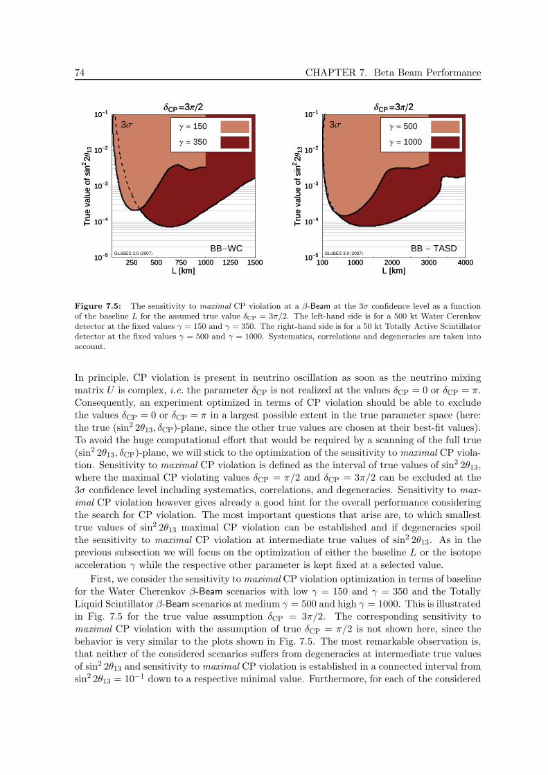
74 CHAPTER 7. Beta Beam Performance

250 500 750 1000 1250 1500L @kmD

10-5

10-4

10-3

10-2

10-1

Tru

eva

lue

ofsi

n22Θ

13

∆CP =3Π2

BB-WCGLoBES 3.0 H2007L

Γ = 150

Γ = 350

3Σ

250 500 750 1000 1250 1500L @kmD

10-5

10-4

10-3

10-2

10-1

Tru

eva

lue

ofsi

n22Θ

13

∆CP =3Π2

100 1000 2000 3000 4000L @kmD

10-5

10-4

10-3

10-2

10-1

Tru

eva

lue

ofsi

n22Θ

13

∆CP =3Π2

BB - TASDGLoBES 3.0 H2007L

Γ = 500

Γ = 1000

3Σ

100 1000 2000 3000 4000L @kmD

10-5

10-4

10-3

10-2

10-1

Tru

eva

lue

ofsi

n22Θ

13

∆CP =3Π2

Figure 7.5: The sensitivity to maximal CP violation at a β-Beam at the 3σ confidence level as a functionof the baseline L for the assumed true value δCP = 3π/2. The left-hand side is for a 500 kt Water Cerenkovdetector at the fixed values γ = 150 and γ = 350. The right-hand side is for a 50 kt Totally Active Scintillatordetector at the fixed values γ = 500 and γ = 1000. Systematics, correlations and degeneracies are taken intoaccount.

In principle, CP violation is present in neutrino oscillation as soon as the neutrino mixingmatrix U is complex, i.e. the parameter δCP is not realized at the values δCP = 0 or δCP = π.Consequently, an experiment optimized in terms of CP violation should be able to excludethe values δCP = 0 or δCP = π in a largest possible extent in the true parameter space (here:the true (sin2 2θ13, δCP)-plane, since the other true values are chosen at their best-fit values).To avoid the huge computational effort that would be required by a scanning of the full true(sin2 2θ13, δCP)-plane, we will stick to the optimization of the sensitivity to maximal CP viola-tion. Sensitivity to maximal CP violation is defined as the interval of true values of sin2 2θ13,where the maximal CP violating values δCP = π/2 and δCP = 3π/2 can be excluded at the3σ confidence level including systematics, correlations, and degeneracies. Sensitivity to max-imal CP violation however gives already a good hint for the overall performance consideringthe search for CP violation. The most important questions that arise are, to which smallesttrue values of sin2 2θ13 maximal CP violation can be established and if degeneracies spoilthe sensitivity to maximal CP violation at intermediate true values of sin2 2θ13. As in theprevious subsection we will focus on the optimization of either the baseline L or the isotopeacceleration γ while the respective other parameter is kept fixed at a selected value.

First, we consider the sensitivity to maximal CP violation optimization in terms of baselinefor the Water Cherenkov β-Beam scenarios with low γ = 150 and γ = 350 and the TotallyLiquid Scintillator β-Beam scenarios at medium γ = 500 and high γ = 1000. This is illustratedin Fig. 7.5 for the true value assumption δCP = 3π/2. The corresponding sensitivity tomaximal CP violation with the assumption of true δCP = π/2 is not shown here, since thebehavior is very similar to the plots shown in Fig. 7.5. The most remarkable observation is,that neither of the considered scenarios suffers from degeneracies at intermediate true valuesof sin2 2θ13 and sensitivity to maximal CP violation is established in a connected interval fromsin2 2θ13 = 10−1 down to a respective minimal value. Furthermore, for each of the considered

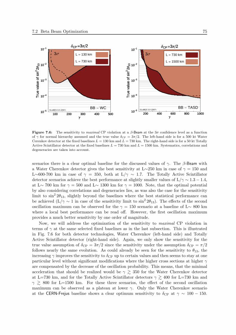
7.2 Beta Beam Optimization 75

100 200 300 400 500Γ

10-5

10-4

10-3

10-2

10-1

Tru

eva

lue

ofsi

n22Θ

13

∆CP =3Π2

BB - WCGLoBES 3.0 H2007L

L = 130 km

L = 730 km

3Σ

100 200 300 400 500Γ

10-5

10-4

10-3

10-2

10-1

Tru

eva

lue

ofsi

n22Θ

13

∆CP =3Π2

200 400 600 800 1000Γ

10-5

10-4

10-3

10-2

10-1

Tru

eva

lue

ofsi

n22Θ

13

∆CP =3Π2

BB - TASDGLoBES 3.0 H2007L

L = 730 km

L = 1500 km

3Σ

200 400 600 800 1000Γ

10-5

10-4

10-3

10-2

10-1

Tru

eva

lue

ofsi

n22Θ

13

∆CP =3Π2

Figure 7.6: The sensitivity to maximal CP violation at a β-Beam at the 3σ confidence level as a functionof γ for normal hierarchy assumed and the true value δCP = 3π/2. The left-hand side is for a 500 kt WaterCerenkov detector at the fixed baselines L = 130 km and L = 730 km. The right-hand side is for a 50 kt TotallyActive Scintillator detector at the fixed baselines L = 730 km and L = 1500 km. Systematics, correlations anddegeneracies are taken into account.

scenarios there is a clear optimal baseline for the discussed values of γ. The β-Beam witha Water Cherenkov detector gives the best sensitivity at L∼250 km in case of γ = 150 andL∼600-700 km in case of γ = 350, both at L/γ ∼ 1.7. The Totally Active Scintillatordetector scenarios achieve the best performance at slightly smaller values of L/γ ∼ 1.3 − 1.4,at L∼ 700 km for γ = 500 and L∼ 1300 km for γ = 1000. Note, that the optimal potentialby also considering correlations and degeneracies lies, as was also the case for the sensitivitylimit to sin2 2θ13, slightly beyond the baselines where the best statistical performance canbe achieved (L/γ ∼ 1 in case of the sensitivity limit to sin2 2θ13). The effects of the secondoscillation maximum can be observed for the γ = 150 scenario at a baseline of L∼ 800 kmwhere a local best performance can be read off. However, the first oscillation maximumprovides a much better sensitivity by one order of magnitude.

Now, we will address the optimization of the sensitivity to maximal CP violation interms of γ at the same selected fixed baselines as in the last subsection. This is illustratedin Fig. 7.6 for both detector technologies, Water Cherenkov (left-hand side) and TotallyActive Scintillator detector (right-hand side). Again, we only show the sensitivity for thetrue value assumption of δCP = 3π/2 since the sensitivity under the assumption δCP = π/2follows nearly the same evolution. As could already be seen for the sensitivity to θ13, theincreasing γ improves the sensitivity to δCP up to certain values and then seems to stay at oneparticular level without significant modifications where the higher cross sections at higher γare compensated by the decrease of the oscillation probability. This means, that the minimalacceleration that should be realized would be γ & 350 for the Water Cherenkov detectorat L=730 km, and for the Totally Active Scintillator detectors γ & 400 for L=730 km andγ & 800 for L=1500 km. For these three scenarios, the effect of the second oscillationmaximum can be observed as a plateau at lower γ. Only the Water Cherenkov scenarioat the CERN-Frejus baseline shows a clear optimum sensitivity to δCP at γ ∼ 100 − 150.

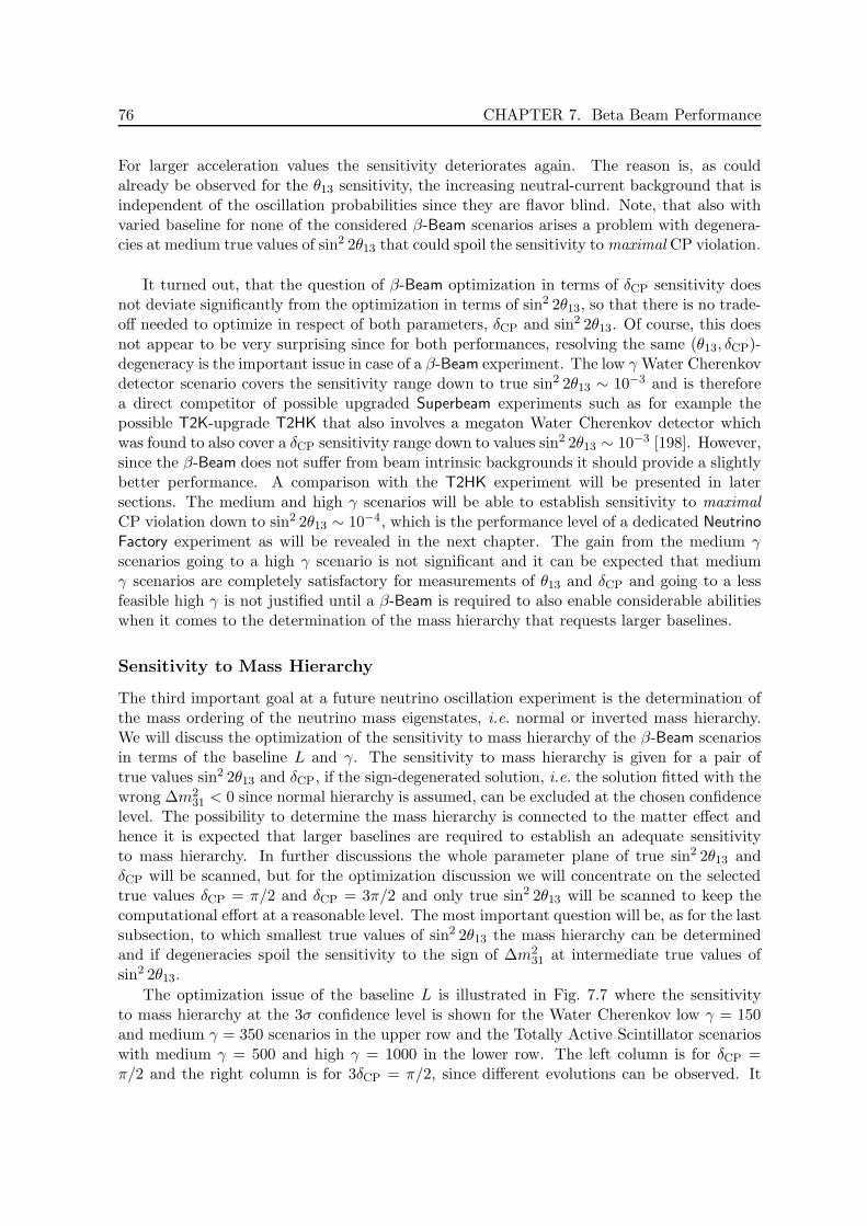
76 CHAPTER 7. Beta Beam Performance

For larger acceleration values the sensitivity deteriorates again. The reason is, as couldalready be observed for the θ13 sensitivity, the increasing neutral-current background that isindependent of the oscillation probabilities since they are flavor blind. Note, that also withvaried baseline for none of the considered β-Beam scenarios arises a problem with degenera-cies at medium true values of sin2 2θ13 that could spoil the sensitivity to maximal CP violation.

It turned out, that the question of β-Beam optimization in terms of δCP sensitivity doesnot deviate significantly from the optimization in terms of sin2 2θ13, so that there is no trade-off needed to optimize in respect of both parameters, δCP and sin2 2θ13. Of course, this doesnot appear to be very surprising since for both performances, resolving the same (θ13, δCP)-degeneracy is the important issue in case of a β-Beam experiment. The low γ Water Cherenkovdetector scenario covers the sensitivity range down to true sin2 2θ13 ∼ 10−3 and is thereforea direct competitor of possible upgraded Superbeam experiments such as for example thepossible T2K-upgrade T2HK that also involves a megaton Water Cherenkov detector whichwas found to also cover a δCP sensitivity range down to values sin2 2θ13 ∼ 10−3 [198]. However,since the β-Beam does not suffer from beam intrinsic backgrounds it should provide a slightlybetter performance. A comparison with the T2HK experiment will be presented in latersections. The medium and high γ scenarios will be able to establish sensitivity to maximalCP violation down to sin2 2θ13 ∼ 10−4, which is the performance level of a dedicated NeutrinoFactory experiment as will be revealed in the next chapter. The gain from the medium γscenarios going to a high γ scenario is not significant and it can be expected that mediumγ scenarios are completely satisfactory for measurements of θ13 and δCP and going to a lessfeasible high γ is not justified until a β-Beam is required to also enable considerable abilitieswhen it comes to the determination of the mass hierarchy that requests larger baselines.

Sensitivity to Mass Hierarchy

The third important goal at a future neutrino oscillation experiment is the determination ofthe mass ordering of the neutrino mass eigenstates, i.e. normal or inverted mass hierarchy.We will discuss the optimization of the sensitivity to mass hierarchy of the β-Beam scenariosin terms of the baseline L and γ. The sensitivity to mass hierarchy is given for a pair oftrue values sin2 2θ13 and δCP, if the sign-degenerated solution, i.e. the solution fitted with thewrong ∆m2

31 < 0 since normal hierarchy is assumed, can be excluded at the chosen confidencelevel. The possibility to determine the mass hierarchy is connected to the matter effect andhence it is expected that larger baselines are required to establish an adequate sensitivityto mass hierarchy. In further discussions the whole parameter plane of true sin2 2θ13 andδCP will be scanned, but for the optimization discussion we will concentrate on the selectedtrue values δCP = π/2 and δCP = 3π/2 and only true sin2 2θ13 will be scanned to keep thecomputational effort at a reasonable level. The most important question will be, as for the lastsubsection, to which smallest true values of sin2 2θ13 the mass hierarchy can be determinedand if degeneracies spoil the sensitivity to the sign of ∆m2

31 at intermediate true values ofsin2 2θ13.

The optimization issue of the baseline L is illustrated in Fig. 7.7 where the sensitivityto mass hierarchy at the 3σ confidence level is shown for the Water Cherenkov low γ = 150and medium γ = 350 scenarios in the upper row and the Totally Active Scintillator scenarioswith medium γ = 500 and high γ = 1000 in the lower row. The left column is for δCP =π/2 and the right column is for 3δCP = π/2, since different evolutions can be observed. It

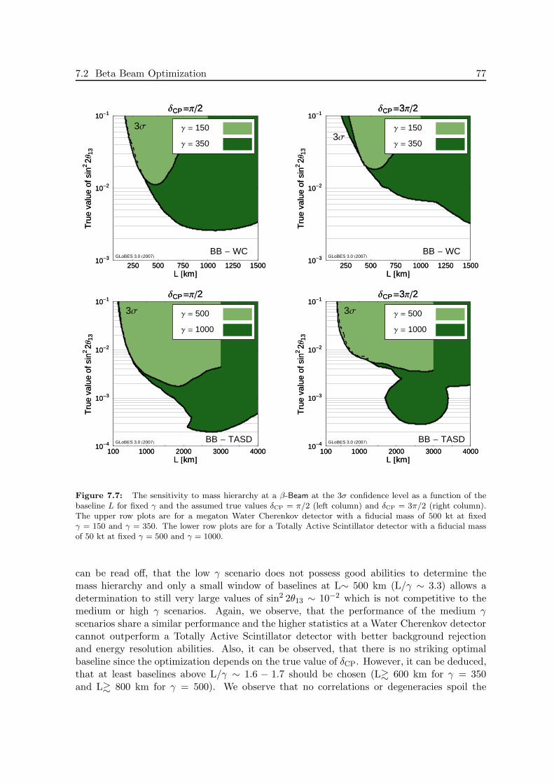
7.2 Beta Beam Optimization 77

250 500 750 1000 1250 1500L @kmD

10-3

10-2

10-1

Tru

eva

lue

ofsi

n22Θ

13

∆CP =Π2

BB - WCGLoBES 3.0 H2007L

Γ = 150

Γ = 350

3Σ

250 500 750 1000 1250 1500L @kmD

10-3

10-2

10-1

Tru

eva

lue

ofsi

n22Θ

13

∆CP =Π2

250 500 750 1000 1250 1500L @kmD

10-3

10-2

10-1

Tru

eva

lue

ofsi

n22Θ

13

∆CP =3Π2

BB - WCGLoBES 3.0 H2007L

Γ = 150

Γ = 3503Σ

250 500 750 1000 1250 1500L @kmD

10-3

10-2

10-1

Tru

eva

lue

ofsi

n22Θ

13

∆CP =3Π2

100 1000 2000 3000 4000L @kmD

10-4

10-3

10-2

10-1

Tru

eva

lue

ofsi

n22Θ

13

∆CP =Π2

BB - TASDGLoBES 3.0 H2007L

Γ = 500

Γ = 1000

3Σ

100 1000 2000 3000 4000L @kmD

10-4

10-3

10-2

10-1

Tru

eva

lue

ofsi

n22Θ

13

∆CP =Π2

100 1000 2000 3000 4000L @kmD

10-4

10-3

10-2

10-1T

rue

valu

eof

sin2

2Θ13

∆CP =3Π2

BB - TASDGLoBES 3.0 H2007L

Γ = 500

Γ = 1000

3Σ

100 1000 2000 3000 4000L @kmD

10-4

10-3

10-2

10-1T

rue

valu

eof

sin2

2Θ13

∆CP =3Π2

Figure 7.7: The sensitivity to mass hierarchy at a β-Beam at the 3σ confidence level as a function of thebaseline L for fixed γ and the assumed true values δCP = π/2 (left column) and δCP = 3π/2 (right column).The upper row plots are for a megaton Water Cherenkov detector with a fiducial mass of 500 kt at fixedγ = 150 and γ = 350. The lower row plots are for a Totally Active Scintillator detector with a fiducial massof 50 kt at fixed γ = 500 and γ = 1000.

can be read off, that the low γ scenario does not possess good abilities to determine themass hierarchy and only a small window of baselines at L∼ 500 km (L/γ ∼ 3.3) allows adetermination to still very large values of sin2 2θ13 ∼ 10−2 which is not competitive to themedium or high γ scenarios. Again, we observe, that the performance of the medium γscenarios share a similar performance and the higher statistics at a Water Cherenkov detectorcannot outperform a Totally Active Scintillator detector with better background rejectionand energy resolution abilities. Also, it can be observed, that there is no striking optimalbaseline since the optimization depends on the true value of δCP. However, it can be deduced,that at least baselines above L/γ ∼ 1.6 − 1.7 should be chosen (L& 600 km for γ = 350and L& 800 km for γ = 500). We observe that no correlations or degeneracies spoil the

78 CHAPTER 7. Beta Beam Performance

sensitivity to mass hierarchy at intermediate true values sin2 2θ13. This picture changes ifthe high γ scenario is investigated. Here only a smaller window of baselines is favored:2500 km . L . 3500 km. The evolution as a function of γ is not smooth anymore and thereappear regions, where sensitivity is lost due to correlations and degeneracies. It appears, thatin the range 1000 km . L . 2000 km the sensitivity is lost in small parts of the sin2 2θ13

parameter space. At baselines L∼2000km the sensitivity to mass hierarchy acquires a gap ofsensitivity loss for intermediate sin2 2θ13 ∼ 2 · 10−3 whereas it is restored again for smallervalues of sin2 2θ13 in the case of δCP = 3π/2 (lower right plot in Fig. 7.7). For this choiceof δCP the sensitivity gets lost again for baselines L& 3500 km for the smallest true valuesof sin2 2θ13. However, in the favored baseline window 2500 km . L . 3500 km this scenariocan establish sensitivity to mass hierarchy down to sin2 2θ13 ∼ (2 − 3) · 10−4. This windowtranslates to 2.5 . L/γ . 1.5 which is unfortunately far off the optimal baseline range formeasurements of δCP. Hence, in order to have optimal abilities in both, search for δCP andthe mass hierarchy, a two detector scenario with Totally Active Scintillator detectors at twodifferent baselines should turn out as the optimal scenario. Scenarios with only one detectorcannot be able to optimize performance for both performance aspects.

Finally, we will address the γ optimization for the sensitivity to mass hierarchy in Fig. 7.8.Now, the dependency of the sensitivity to the sign of ∆m2

31 on the isotope acceleration factorγ is illustrated for selected baselines. The upper row shows the performance of the WaterCherenkov detector scenarios at L = 130 km and L = 730 km while the Totally ActiveScintillator detector scenarios at L = 730 km and L = 1500 km are considered in the lowerrow. The L = 130 km scenario suffers from a total lack of sensitivity to the mass hierarchyat any chosen value of γ, so this scenario is only able to provide information on sin2 2θ13 andδCP. Hence, it can be optimized just with respect to these two parameters. Furthermore,if the upper and lower row plots are compared, the medium baseline scenarios share a verysimilar performance independent of the detector technology as turned out to be true alreadyfor the performances if considering θ13 and δCP. The higher baseline of L = 1500 km onlyprovides a small increase in the performance which is not surprising, because it was observedin Fig. 7.7 that only in the window of 2500 km . L . 3500 km very good sensitivities to themass hierarchy can be achieved.

When it comes to a comparison of the performance of β-Beam scenarios with NeutrinoFactory experiments, the sensitivity to mass hierarchy will be crucial point for the mostdedicated5 β-Beam scenarios to compete with the Neutrino Factory that provides for verygood abilities in determining the mass hierarchy due to the very high baselines of severalthousands of kilometers. It is clear, that low γ β-Beam scenarios cannot compete at allwith a Neutrino Factory on this issue and have to be seen as very powerful alternatives toupgraded Superbeams such as T2HK in the search for sin2 2θ13 and δCP. While mediumγ scenarios provide at least some moderate capabilities in determining the mass hierarchy,the ultimate β-Beam optimization in that respect involves a detector at very large baselines2500 km . L . 3500 km which collides for the realistic range of γ with the optimization withrespect to δCP, so a two detector scenario is preferable to assure optimal performance in bothaspects.

5in terms of cost intensiveness

7.2 Beta Beam Optimization 79

100 200 300 400 500Γ

10-3

10-2

10-1

Tru

eva

lue

ofsi

n22Θ

13

∆CP =Π2

BB - WCGLoBES 3.0 H2007L

L=130km

L=730km

3Σ

100 200 300 400 500Γ

10-3

10-2

10-1

Tru

eva

lue

ofsi

n22Θ

13

∆CP =Π2

100 200 300 400 500Γ

10-3

10-2

10-1

Tru

eva

lue

ofsi

n22Θ

13

∆CP =3Π2

BB - WCGLoBES 3.0 H2007L

L=130km

L=730km

3Σ

100 200 300 400 500Γ

10-3

10-2

10-1

Tru

eva

lue

ofsi

n22Θ

13

∆CP =3Π2

200 400 600 800 1000Γ

10-3

10-2

10-1

Tru

eva

lue

ofsi

n22Θ

13

∆CP =Π2

BB - TASDGLoBES 3.0 H2007L

L=730km

L=1500km

3Σ

200 400 600 800 1000Γ

10-3

10-2

10-1

Tru

eva

lue

ofsi

n22Θ

13

∆CP =Π2

200 400 600 800 1000Γ

10-3

10-2

10-1T

rue

valu

eof

sin2

2Θ13

∆CP =3Π2

BB - TASDGLoBES 3.0 H2007L

L=730km

L=1500km

3Σ

200 400 600 800 1000Γ

10-3

10-2

10-1T

rue

valu

eof

sin2

2Θ13

∆CP =3Π2

Figure 7.8: The sensitivity to mass hierarchy at a β-Beam at the 3σ confidence level as a function of γ for afixed baseline L and the assumed true values δCP = π/2 (left column) and δCP = 3π/2 (right column). NormalHierarchy is assumed. The upper plots are for a megaton Water Cherenkov detector with a fiducial mass of500 kt at fixed L = 130 km and L = 730 km. The lower row plots are for a Totally Active Scintillatordetector with a fiducial mass of 50 kt at fixed L = 730 km and L = 1500 km.

β-Beam Reference Scenarios

The last subsections focused on the independent optimization of different β-Beam scenariosin terms of baseline L and γ. We will now assign defined reference setups that follow thesuggestions from the optimization discussions and provide the possibility to study the prop-erties and performances in a greater detail. Furthermore, these defined reference setups andtheir abilities can be comfortably compared to reference setups of different technologies, e.g.Neutrino Factory setups or the Superbeam upgrade T2HK. These reference setups shall coverall three ranges of γ, low, medium and high, and the two discussed detector technologies inthe compatible γ range. The definition of the reference setups is based slightly more uponthe discussion of γ-optimization since the selected baselines that were discussed there are

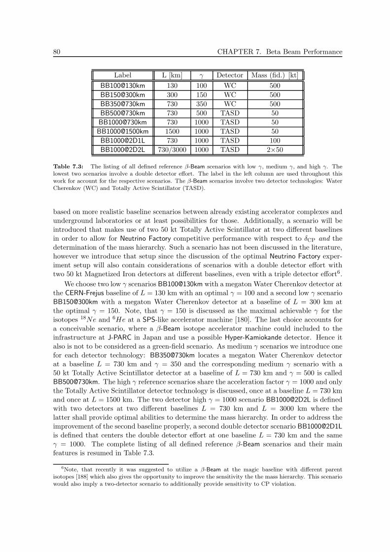
80 CHAPTER 7. Beta Beam Performance

Label L [km] γ Detector Mass (fid.) [kt]

BB100@130km 130 100 WC 500

BB150@300km 300 150 WC 500

BB350@730km 730 350 WC 500

BB500@730km 730 500 TASD 50

BB1000@730km 730 1000 TASD 50

BB1000@1500km 1500 1000 TASD 50

BB1000@2D1L 730 1000 TASD 100

BB1000@2D2L 730/3000 1000 TASD 2×50

Table 7.3: The listing of all defined reference β-Beam scenarios with low γ, medium γ, and high γ. Thelowest two scenarios involve a double detector effort. The label in the left column are used throughout thiswork for account for the respective scenarios. The β-Beam scenarios involve two detector technologies: WaterCherenkov (WC) and Totally Active Scintillator (TASD).

based on more realistic baseline scenarios between already existing accelerator complexes andunderground laboratories or at least possibilities for those. Additionally, a scenario will beintroduced that makes use of two 50 kt Totally Active Scintillator at two different baselinesin order to allow for Neutrino Factory competitive performance with respect to δCP and thedetermination of the mass hierarchy. Such a scenario has not been discussed in the literature,however we introduce that setup since the discussion of the optimal Neutrino Factory exper-iment setup will also contain considerations of scenarios with a double detector effort withtwo 50 kt Magnetized Iron detectors at different baselines, even with a triple detector effort6.

We choose two low γ scenarios BB100@130km with a megaton Water Cherenkov detector atthe CERN-Frejus baseline of L = 130 km with an optimal γ = 100 and a second low γ scenarioBB150@300km with a megaton Water Cherenkov detector at a baseline of L = 300 km atthe optimal γ = 150. Note, that γ = 150 is discussed as the maximal achievable γ for theisotopes 18Ne and 6He at a SPS-like accelerator machine [180]. The last choice accounts fora conceivable scenario, where a β-Beam isotope accelerator machine could included to theinfrastructure at J-PARC in Japan and use a possible Hyper-Kamiokande detector. Hence italso is not to be considered as a green-field scenario. As medium γ scenarios we introduce onefor each detector technology: BB350@730km locates a megaton Water Cherenkov detectorat a baseline L = 730 km and γ = 350 and the corresponding medium γ scenario with a50 kt Totally Active Scintillator detector at a baseline of L = 730 km and γ = 500 is calledBB500@730km. The high γ reference scenarios share the acceleration factor γ = 1000 and onlythe Totally Active Scintillator detector technology is discussed, once at a baseline L = 730 kmand once at L = 1500 km. The two detector high γ = 1000 scenario BB1000@2D2L is definedwith two detectors at two different baselines L = 730 km and L = 3000 km where thelatter shall provide optimal abilities to determine the mass hierarchy. In order to address theimprovement of the second baseline properly, a second double detector scenario BB1000@2D1Lis defined that centers the double detector effort at one baseline L = 730 km and the sameγ = 1000. The complete listing of all defined reference β-Beam scenarios and their mainfeatures is resumed in Table 7.3.

6Note, that recently it was suggested to utilize a β-Beam at the magic baseline with different parentisotopes [188] which also gives the opportunity to improve the sensitivity the the mass hierarchy. This scenariowould also imply a two-detector scenario to additionally provide sensitivity to CP violation.

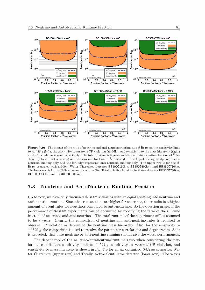
7.3 Neutrino and Anti-Neutrino Runtime Fraction 81

0 0.2 0.4 0.6 0.8 1

Runtime fraction -18Ne stored

10-5

10-4

10-3

10-2

10-1

Rea

chin

sin2

2Θ13

BB100130km - WC

3ΣGLoBES 3.0 H2007L

Mass hierarchy

CP violation

sin2 2Θ13 limit

0 0.2 0.4 0.6 0.8 1

Runtime fraction -18Ne stored

10-5

10-4

10-3

10-2

10-1

Rea

chin

sin2

2Θ13

BB100130km - WC

0 0.2 0.4 0.6 0.8 1

Runtime fraction -18Ne stored

10-5

10-4

10-3

10-2

10-1

Rea

chin

sin2

2Θ13

BB150300km - WC

3ΣGLoBES 3.0 H2007L

Mass hierarchy

CP violation

sin2 2Θ13 limit

0 0.2 0.4 0.6 0.8 1

Runtime fraction -18Ne stored

10-5

10-4

10-3

10-2

10-1

Rea

chin

sin2

2Θ13

BB150300km - WC

0 0.2 0.4 0.6 0.8 1

Runtime fraction -18Ne stored

10-5

10-4

10-3

10-2

10-1

Rea

chin

sin2

2Θ13

BB350730km - WC

3ΣGLoBES 3.0 H2007L

sin2 2Θ13 limit

CP violation

Mass hierarchy

0 0.2 0.4 0.6 0.8 1

Runtime fraction -18Ne stored

10-5

10-4

10-3

10-2

10-1

Rea

chin

sin2

2Θ13

BB350730km - WC

0 0.2 0.4 0.6 0.8 1

Runtime fraction -18Ne stored

10-5

10-4

10-3

10-2

10-1

Rea

chin

sin2

2Θ13

BB500730km - TASD

3ΣGLoBES 3.0 H2007L

sin2 2Θ13 limit

CP violation

Mass hierarchy

0 0.2 0.4 0.6 0.8 1

Runtime fraction -18Ne stored

10-5

10-4

10-3

10-2

10-1

Rea

chin

sin2

2Θ13

BB500730km - TASD

0 0.2 0.4 0.6 0.8 1

Runtime fraction -18Ne stored

10-5

10-4

10-3

10-2

10-1

Rea

chin

sin2

2Θ13

BB1000730km - TASD

3ΣGLoBES 3.0 H2007L

sin2 2Θ13 limit

CP violation

Mass hierarchy

0 0.2 0.4 0.6 0.8 1

Runtime fraction -18Ne stored

10-5

10-4

10-3

10-2

10-1

Rea

chin

sin2

2Θ13

BB1000730km - TASD

0 0.2 0.4 0.6 0.8 1

Runtime fraction -18Ne stored

10-5

10-4

10-3

10-2

10-1

Rea

chin

sin2

2Θ13

BB10001500km - TASD

3ΣGLoBES 3.0 H2007L

sin2 2Θ13 limit

CP violation

Mass hierarchy

0 0.2 0.4 0.6 0.8 1

Runtime fraction -18Ne stored

10-5

10-4

10-3

10-2

10-1

Rea

chin

sin2

2Θ13

BB10001500km - TASD

Figure 7.9: The impact of the ratio of neutrino and anti-neutrino runtime at a β-Beam on the sensitivity limitto sin2 2θ13 (left), the sensitivity to maximal CP violation (middle), and sensitivity to the mass hierarchy (right)at the 3σ confidence level respectively. The total runtime is 8 years and divided into a runtime fraction of 18Nestored (labeled on the x-axis) and the runtime fraction of 6He stored. In each plot the right edge representsneutrino running only and the left edge represents anti-neutrino running only. The upper row is for the β-

Beam scenarios with a 500kt Water Cherenkov detector BB100@130km, BB150@300km, and BB350@730km.The lower row is for the β-Beam scenarios with a 50kt Totally Active Liquid scintillator detector BB500@730km,BB1000@730km, and BB1000@1500km.

7.3 Neutrino and Anti-Neutrino Runtime Fraction

Up to now, we have only discussed β-Beam scenarios with an equal splitting into neutrino andanti-neutrino runtime. Since the cross sections are higher for neutrinos, this results in a higheramount of event rates for neutrinos compared to anti-neutrinos. So the question arises, if theperformance of β-Beam experiments can be optimized by modifying the ratio of the runtimefraction of neutrinos and anti-neutrinos. The total runtime of the experiment still is assumedto be 8 years. Clearly, the comparison of neutrino and anti-neutrino rates is required toobserve CP violation or determine the neutrino mass hierarchy. Also, for the sensitivity tosin2 2θ13 the comparison is used to resolve the parameter correlations and degeneracies. So itis expected, that pure neutrino or anti-neutrino running should give the worst performances.

The dependence of the neutrino/anti-neutrino runtime ratio when considering the per-formance indicators sensitivity limit to sin2 2θ13, sensitivity to maximal CP violation, andsensitivity to mass hierarchy is shown in Fig. 7.9 for all six optimized β-Beam scenarios, Wa-ter Cherenkov (upper row) and Totally Active Scintillator detector (lower row). The x-axis

82 CHAPTER 7. Beta Beam Performance

indicates the neutrino runtime fraction f(18Ne), i.e. the fraction of the phase with 18Neisotopes stored in the storage rings compared to the total runtime of the experiment. Theanti-neutrino runtime fraction f(6He), i.e. the phase with 6He isotopes stored in the storagering is the given by f(6He) = 1−f(18Ne). Thus, the left edge of the respective plots describesthe performance with anti-neutrino running only and the right edge describes the performancewith pure neutrino running. The middle position of each plot with f(18Ne) = f(6He) = 0.5corresponds to the scenarios discussed up to now with an equal amount of runtime for neu-trinos and anti-neutrinos. As expected the performance drops visibly to the outer regions ofthe respective plots. However, for neutrino runtime fraction 0.2 . f(18Ne) . 0.8 the perfor-mances for all three discussed performance indicators are approximately independent of theactual ratio between neutrino and anti-neutrino runtime. There could be a slight individualoptimization for the scenarios, but it turns out that appointing an equal runtime of neutrinosand anti-neutrinos is on average the best choice and has not to be modified. Consequently,throughout the rest of this work we will stick to the assumption of f(18Ne) = f(6He) = 0.5and keep the equal runtimes for neutrinos and anti-neutrinos.

The results from Fig. 7.9 can also interpreted in such a way, that the performance of theβ-Beam does not depend so crucially on the requirement that the number of isotope decaysper year has to be achieved as planned. If, for some reason, for one of the isotopes the plannednumber of decays per year can not be technically feasible and a lower number turns out tobe realistic, this could be compensated by an increase of the number of decays of the otherisotope (see [235] for issues of feasibility).

7.4 Addition of T2K Disappearance Data

It was mentioned before, that the leading atmospheric parameters sin2 2θ23 and ∆m231 cannot

be measured at a β-Beam experiment itself. This clearly distinguishes a β-Beam experimentfrom a Neutrino Factory or even Superbeams where information on the leading atmosphericparameters can be obtained by the observation of the νµ-disappearance, whereas at a β-Beamexperiment only the disappearance of νe could be measured in addition to the appearancedata. Since the corresponding disappearance is driven by the parameters sin2 2θ13 and ∆m2

31

there cannot be extracted any information on sin2 2θ23. Furthermore, since the amplitude issin2 2θ13, which is known to be small, the usefulness of the νe-disappearance data dependscrucially on the systematical uncertainties. This effect is known very well from reactor experi-ments where νe-disappearance is observed and the achievable sensitivity to sin2 2θ13 is limitedby the systematical uncertainties concerning for instance the reactor flux normalization, thecross sections, the fiducial volumes of the detector or even bin-to-bin errors like uncertaintiesin the reactor flux spectrum. It is well known, that these uncertainties have to be kept at theorder of 1% or below to improve the current limits on sin2 2θ13 [155]. However, at beam exper-iments like at a β-Beam it is hardly achievable to arrive at such low systematical uncertainties.In fact, the assumption of 2.5% uncertainty on the number of signal events has already to beviewed as slightly optimistic. Consequently, it is not to be expected that the performance of aβ-Beam is affected by the inclusion of the disappearance data. Although this is not explicitlyshown in this work, we checked that indeed all later discussed β-Beam scenarios arrive atthe same sin2 2θ13, δCP, and mass hierarchy sensitivities, whether the disappearance data isincluded or not.

Thus, neither sin2 2θ23 nor ∆m231 can be measured at a β-Beam experiment. It was previ-

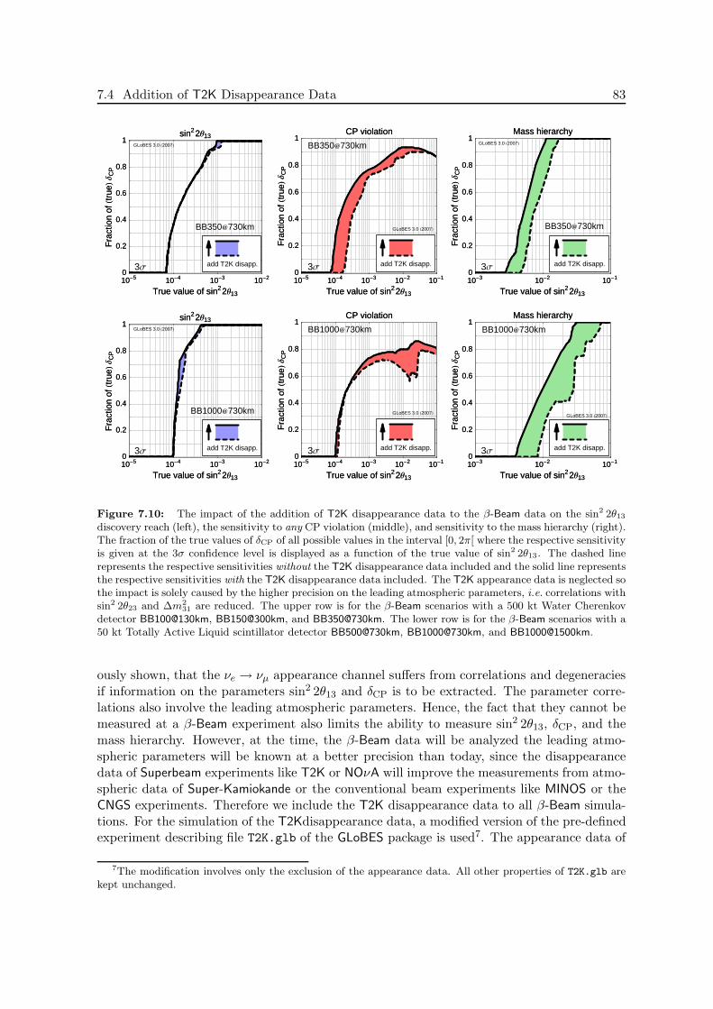
7.4 Addition of T2K Disappearance Data 83

10-210-310-410-5

True value of sin22Θ13

0

0.2

0.4

0.6

0.8

1

Fra

ctio

nofHt

rueL

∆C

P

sin22Θ13

add T2K disapp.

GLoBES 3.0 H2007L

3Σ

BB350730km

10-210-310-410-5

True value of sin22Θ13

0

0.2

0.4

0.6

0.8

1

Fra

ctio

nofHt

rueL

∆C

P

sin22Θ13

10-110-210-310-410-5

True value of sin22Θ13

0

0.2

0.4

0.6

0.8

1

Fra

ctio

nofHt

rueL

∆C

P

CP violation

add T2K disapp.

GLoBES 3.0 H2007L

3Σ

BB350730km

10-110-210-310-410-5

True value of sin22Θ13

0

0.2

0.4

0.6

0.8

1

Fra

ctio

nofHt

rueL

∆C

P

CP violation

10-110-210-3

True value of sin22Θ13

0

0.2

0.4

0.6

0.8

1

Fra

ctio

nofHt

rueL

∆C

P

Mass hierarchy

add T2K disapp.

GLoBES 3.0 H2007L

3Σ

BB350730km

10-110-210-3

True value of sin22Θ13

0

0.2

0.4

0.6

0.8

1

Fra

ctio

nofHt

rueL

∆C

P

Mass hierarchy

10-210-310-410-5

True value of sin22Θ13

0

0.2

0.4

0.6

0.8

1

Fra

ctio

nofHt

rueL

∆C

P

sin22Θ13

add T2K disapp.

GLoBES 3.0 H2007L

3Σ

BB1000730km

10-210-310-410-5

True value of sin22Θ13

0

0.2

0.4

0.6

0.8

1

Fra

ctio

nofHt

rueL

∆C

P

sin22Θ13

10-110-210-310-410-5

True value of sin22Θ13

0

0.2

0.4

0.6

0.8

1

Fra

ctio

nofHt

rueL

∆C

P

CP violation

add T2K disapp.

GLoBES 3.0 H2007L

3Σ

BB1000730km

10-110-210-310-410-5

True value of sin22Θ13

0

0.2

0.4

0.6

0.8

1

Fra

ctio

nofHt

rueL

∆C

P

CP violation

10-110-210-3

True value of sin22Θ13

0

0.2

0.4

0.6

0.8

1

Fra

ctio

nofHt

rueL

∆C

P

Mass hierarchy

add T2K disapp.

GLoBES 3.0 H2007L

3Σ

BB1000730km

10-110-210-3

True value of sin22Θ13

0

0.2

0.4

0.6

0.8

1

Fra

ctio

nofHt

rueL

∆C

P

Mass hierarchy

Figure 7.10: The impact of the addition of T2K disappearance data to the β-Beam data on the sin2 2θ13

discovery reach (left), the sensitivity to any CP violation (middle), and sensitivity to the mass hierarchy (right).The fraction of the true values of δCP of all possible values in the interval [0, 2π[ where the respective sensitivityis given at the 3σ confidence level is displayed as a function of the true value of sin2 2θ13. The dashed linerepresents the respective sensitivities without the T2K disappearance data included and the solid line representsthe respective sensitivities with the T2K disappearance data included. The T2K appearance data is neglected sothe impact is solely caused by the higher precision on the leading atmospheric parameters, i.e. correlations withsin2 2θ23 and ∆m2

31 are reduced. The upper row is for the β-Beam scenarios with a 500 kt Water Cherenkovdetector BB100@130km, BB150@300km, and BB350@730km. The lower row is for the β-Beam scenarios with a50 kt Totally Active Liquid scintillator detector BB500@730km, BB1000@730km, and BB1000@1500km.

ously shown, that the νe → νµ appearance channel suffers from correlations and degeneraciesif information on the parameters sin2 2θ13 and δCP is to be extracted. The parameter corre-lations also involve the leading atmospheric parameters. Hence, the fact that they cannot bemeasured at a β-Beam experiment also limits the ability to measure sin2 2θ13, δCP, and themass hierarchy. However, at the time, the β-Beam data will be analyzed the leading atmo-spheric parameters will be known at a better precision than today, since the disappearancedata of Superbeam experiments like T2K or NOνA will improve the measurements from atmo-spheric data of Super-Kamiokande or the conventional beam experiments like MINOS or theCNGS experiments. Therefore we include the T2K disappearance data to all β-Beam simula-tions. For the simulation of the T2Kdisappearance data, a modified version of the pre-definedexperiment describing file T2K.glb of the GLoBES package is used7. The appearance data of

7The modification involves only the exclusion of the appearance data. All other properties of T2K.glb arekept unchanged.

84 CHAPTER 7. Beta Beam Performance

T2K is excluded so that all sensitivities to sin2 2θ13, δCP, and the mass hierarchy are solelyobtained from the β-Beam appearance data. The same technique has already been used inthe β-Beam simulations in ( [186,236]).

The impact of the inclusion of the T2K disappearance data is exemplary shown in Fig. 7.10for the discovery reach in sin2 2θ13 (left plot), sensitivity to any CP violation (middle plot),and sensitivity to mass hierarchy (right plot) for the a selected β-Beam scenario with a WaterCherenkov detector in the upper row (BB350@730km) and one with a Totally Active Scin-tillator detector in the lower row (BB1000@730km). In each plot, the dashed line depictsthe performance for the β-Beam scenarios alone without the T2K disappearance data. Theimprovement of the inclusion of the T2K disappearance data is indicated by the grey shadedarea up to the solid line that indicates the performance of the β-Beam scenarios if the T2Kdisappearance data is included to the analysis. The discovery reach in sin2 2θ13 turns outto be quite robust for both the considered β-Beam scenarios, but the sensitivities to anyCP violation and mass hierarchy are indeed strongly improved by the inclusion of the T2Kdisappearance data.

7.5 γ-Scaling of the Isotope Decays

We have already mentioned that the number of decays per year is most likely not constantin γ. In order to include this effect, we use the following power law parameterization, whichshould be justified for a certain γ-range, to describe this scaling with γ (i = 1 for 18Ne:neutrinos, i = 2 for 6He: anti-neutrinos):

N i = N i0 ·(

γi0

γ

)n

(7.1)

Here N i0 is determined by our reference point at γ1

0 = 100, γ20 = 60. We can now discuss

different cases for n, which leads to different optimization strategies:

• n = 0: The number of decays per year is fixed. This implies that the accelerator andstorage ring has to scale appropriately with γ in a non-trivial manner.

• 0 < n < 1: This seems to be the most likely range of realistic cases. The number ofdecays per year becomes constrained with increasing γ by the geometry of the acceleratorand decay ring and γ increased lifetime of the isotopes in the laboratory system.

• n ∼ 1: This case corresponds to a fixed setup constraining the performance. A realisticconstraint for the SPS would be, for example, n ∼ 1 from the number of merges in thedecay ring and the number of ions per bunch [235].

• n > 1: In this case, it clearly does not make sense to go to higher γ’s, since the eventrate decreases with γ if we stay in the oscillation maximum

• n < 0: The number of decays per year increases with γ. This hypothetical (buttechnologically unlikely) possibility requires that the accelerator and decay ring over-proportionally scale with γ.

We further on consider the range 0 . n . 1 to be realistic. However, it is conceivable that,for a given setup, the performance will scale with n ≃ 0 in the beginning, and change into an

7.5 γ-Scaling of the Isotope Decays 85

10-110-210-310-410-5

True value of sin22Θ13

0

0.2

0.4

0.6

0.8

1

Fra

ctio

nofHt

rueL

∆C

P

sin22Θ13

n=0n=0.5n=1

GLoBES 3.0 H2007L

3Σ

BB350730km

10-110-210-310-410-5

True value of sin22Θ13

0

0.2

0.4

0.6

0.8

1

Fra

ctio

nofHt

rueL

∆C

P

sin22Θ13

10-110-210-310-410-5

True value of sin22Θ13

0

0.2

0.4

0.6

0.8

1

Fra

ctio

nofHt

rueL

∆C

P

CP violation

n=0n=0.5n=1

GLoBES 3.0 H2007L

3Σ

BB350730km

10-110-210-310-410-5

True value of sin22Θ13

0

0.2

0.4

0.6

0.8

1

Fra

ctio

nofHt

rueL

∆C

P

CP violation

10-110-210-3

True value of sin22Θ13

0

0.2

0.4

0.6

0.8

1

Fra

ctio

nofHt

rueL

∆C

P

Mass hierarchy

n=0n=0.5n=1

GLoBES 3.0 H2007L3Σ

BB350730km

10-110-210-3

True value of sin22Θ13

0

0.2

0.4

0.6

0.8

1

Fra

ctio

nofHt

rueL

∆C

P

Mass hierarchy

10-110-210-310-410-5

True value of sin22Θ13

0

0.2

0.4

0.6

0.8

1

Fra

ctio

nofHt

rueL

∆C

P

sin22Θ13

n=0n=0.5n=1

GLoBES 3.0 H2007L

3Σ

BB1000730km

10-110-210-310-410-5

True value of sin22Θ13

0

0.2

0.4

0.6

0.8

1

Fra

ctio

nofHt

rueL

∆C

P

sin22Θ13

10-110-210-310-410-5

True value of sin22Θ13

0

0.2

0.4

0.6

0.8

1

Fra

ctio

nofHt

rueL

∆C

P

CP violation

n=0n=0.5n=1

GLoBES 3.0 H2007L

3Σ

BB1000730km

10-110-210-310-410-5

True value of sin22Θ13

0

0.2

0.4

0.6

0.8

1

Fra

ctio

nofHt

rueL

∆C

P

CP violation

10-110-210-3

True value of sin22Θ13

0

0.2

0.4

0.6

0.8

1

Fra

ctio

nofHt

rueL

∆C

P

Mass hierarchy

n=0n=0.5n=1

GLoBES 3.0

3Σ

BB1000730km

10-110-210-3

True value of sin22Θ13

0

0.2

0.4

0.6

0.8

1

Fra

ctio

nofHt

rueL

∆C

P

Mass hierarchy

Figure 7.11: The impact of the γ-scaling of the number of isotope decays per year at a β-Beam on thesin2 2θ13 discovery reach (left), the sensitivity to any CP violation (middle), and sensitivity to the masshierarchy (right). The fraction of the true values of δCP of all possible values in the interval [0, 2π[ where therespective sensitivity is given at the 3σ confidence level is displayed as a function of the true value of sin2 2θ13.The number of isotope decays per year is not treated as constant but as a function of γ. It is effectivelydescribed by an exponent n so that the number of isotope decays scales with (1/γ)n (see text for details). Theband indicates the impact of the γ-scaling where the exponent n is varied from n = 0 (solid line, standardassumption) over n = 0.5 (short-dashed line) to n = 1 (long-dashed line). The upper row is for the β-Beam

scenarios with a 500 kt Water Cherenkov detector BB100@130km, BB150@300km, and BB350@730km. Thelower row is for the β-Beam scenarios with a 50 kt Totally Active Liquid scintillator detector BB500@730km,BB1000@730km, and BB1000@1500km.

n ≃ 1 scaling in the saturation regime. In case of n ∼ 1 the γ-scaling would counteract theeffect of higher statistics due to higher cross sections at higher energies. The cross sectionsincrease linearly with the neutrino energies that are proportional to γ but the number ofisotope decays would exactly compensate the effect by the scaling with 1/γ. In this case onlylow γ β-Beams are conceivable since medium and high γ β-Beams additionally require largerbaselines to cover the oscillation maximum and introduce an effective loss in statistics due tothe additional baseline scaling of the events with 1/L2.

We show in Fig. 7.11 the γ-scaling of the performance indicators discovery reach in sin2 2θ13

(left), sensitivity to any CP violation (middle), and sensitivity to the mass hierarchy (right) forthe medium γ Water Cherenkov β-Beam BB350@730km (upper row) and the high γ TotallyActive Scintillator β-Beam BB1000@730km (lower row). The bands indicate the impact ofthe γ-scaling describing parameter 0 ≤ n ≤ 1. The solid upper curves are for n = 0 whichcorresponds to the assumption throughout the rest of this work, while the dashed lines imply

86 CHAPTER 7. Beta Beam Performance

a γ scaling with n = 0.5 (short-dashed curves) and n = 1 (long-dashed curves). The low γβ-Beams are not shown here, because it can be expected that the γ-scaling has no big impactsince the discussed values of γ are close to the reference values γi

0. The effect that the impactof a possible γ-scaling increases with γ can also be observed in Fig. 7.11 by comparing theupper and lower rows. Clearly, the high γ scenario BB1000@730km suffers more severe fromthe γ-scaling than the medium γ scenario BB350@730km. However, also the performanceof BB350@730km is strongly limited if the number of isotope decays cannot be guaranteedby either injecting a larger number of parent isotopes into the storage ring or adjust thearchitecture of the storing ring.

7.6 Performance of the β-Beam Reference Scenarios

The aim of this section is to compare the performance of the optimized reference β-Beamscenarios that have been introduced in Section 7.2. We will focus on the respective abilitiesto discover a non-zero θ13, CP violation, and determine the mass hierarchy in the range fromlarge sin2 2θ13 to very small sin2 2θ13. The goal is to compare the abilities of the possibleβ-Beam scenarios that involve low, medium, and high γ acceleration of the stored isotopesand different detector technologies. The performances of the reference setups are shown inFig. 7.12. The left column represents the discovery reach in sin2 2θ13, the middle columnrepresents the sensitivity to any CP violation, and the right column represents the sensitivityto mass hierarchy, each at the 3σ confidence level. The rows correspond to different detectorefforts. The first row involves a megaton Water Cherenkov detector and the optimized low andmedium γ scenarios. The second row involves a 50 kt Totally Active Scintillator detector thatallows for higher neutrino energies and compares the optimized meed medium and high γ sce-narios. The lowest row represents β-Beam scenarios that involve a double detector effort, i.e.two 50 kt Totally Active Scintillator detectors. The performance is furthermore comparedwith the performance of an upgraded Superbeam experiment T2HK∗8 that is indicated by thegrey area in the plots. Note, that the comparison with T2HK∗ is most interesting for theWater Cherenkov β-Beam scenarios in the first row, since the detector effort is the same sincealso T2HK∗ involves a megaton Water Cherenkov detector, in case of BB150@300km actuallyat a similar baseline.

So, let us first discuss the Water Cherenkov β-Beam scenarios in the first row of Fig. 7.12.It can be observed that the scenarios BB100@130km and BB150@300km do not have signifi-cant abilities to determine the neutrino mass hierarchy due to the relatively small baselines.Also T2HK∗ does not show better sensitivity to the sign of ∆m2

31. The medium γ scenarioBB350@730km on the other hand is able to determine the mass hierarchy in the large regimeof sin2 2θ13 > 10−2 for 100% of all possible values of δCP. If one considers the sensitivity toCP violation the performance of the β-Beams increases with γ and the medium γ scenarioBB350@730km shows excellent sensitivity. For sin2 2θ13 ∼ 10−2 this scenario can establish CPviolation already for more than 90% of all possible values of δCP. Note, that 100% cannotbe reached since CP violation cannot be excluded for values near the CP conserving valuesδCP = 0 and δCP = π. So, BB350@730km is able to perform δCP measurements at very

8The simulation is performed with the GLoBES experiment file T2HK.glb provided with the GLoBES 3.0

package [220] but the fiducial volume is modified to 500 kt instead of 440 kt to be comparable at a fair with theβ-Beam scenarios that involve a Water Cherenkov detector. The modification is indicated by the star followingthe notation from [186] since this is the same scenario that was used there. Further details of the experimentdescription are given in the GLoBES manual [223].

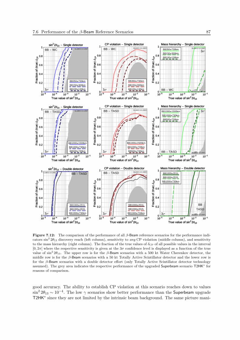
7.6 Performance of the β-Beam Reference Scenarios 87

10-110-210-310-410-5

True value of sin22Θ13

0

0.2

0.4

0.6

0.8

1

Fra

ctio

nofHt

rueL

∆C

P

sin22Θ13 - Single detector

BB100130km

BB150300km

BB350730km

GLoBES 3.0 H2007L

3Σ

BB - WC

10-110-210-310-410-5

True value of sin22Θ13

0

0.2

0.4

0.6

0.8

1

Fra

ctio

nofHt

rueL

∆C

P

sin22Θ13 - Single detector

10-110-210-310-410-5

True value of sin22Θ13

0

0.2

0.4

0.6

0.8

1

Fra

ctio

nofHt

rueL

∆C

P

CP violation - Single detector

BB100130km

BB150300km

BB350730km

GLoBES 3.0 H2007L

3Σ

BB - WC

10-110-210-310-410-5

True value of sin22Θ13

0

0.2

0.4

0.6

0.8

1

Fra

ctio

nofHt

rueL

∆C

P

CP violation - Single detector

10-110-210-310-410-5

True value of sin22Θ13

0

0.2

0.4

0.6

0.8

1

Fra

ctio

nofHt

rueL

∆C

P

Mass hierarchy - Single detector

BB100130km

BB150300km

BB350730km GLoBES 3.0 H2007L

3Σ

BB - WC

10-110-210-310-410-5

True value of sin22Θ13

0

0.2

0.4

0.6

0.8

1

Fra

ctio

nofHt

rueL

∆C

P

Mass hierarchy - Single detector

10-110-210-310-410-5

True value of sin22Θ13

0

0.2

0.4

0.6

0.8

1

Fra

ctio

nofHt

rueL

∆C

P

sin22Θ13 - Single detector

BB500730km

BB1000730km

BB10001500km

GLoBES 3.0 H2007L

3Σ

BB - TASD

10-110-210-310-410-5

True value of sin22Θ13

0

0.2

0.4

0.6

0.8

1

Fra

ctio

nofHt

rueL

∆C

P

sin22Θ13 - Single detector

10-110-210-310-410-5

True value of sin22Θ13

0

0.2

0.4

0.6

0.8

1

Fra

ctio

nofHt

rueL

∆C

P

CP violation - Single detector

BB500730km

BB1000730km

BB10001500km

GLoBES 3.0 H2007L

3Σ

BB - TASD

10-110-210-310-410-5

True value of sin22Θ13

0

0.2

0.4

0.6

0.8

1

Fra

ctio

nofHt

rueL

∆C

P

CP violation - Single detector

10-110-210-310-410-5

True value of sin22Θ13

0

0.2

0.4

0.6

0.8

1

Fra

ctio

nofHt

rueL

∆C

P

Mass hierarchy - Single detector

BB500730km

BB1000730km

BB10001500km

GLoBES 3.0 H2007L

3Σ

BB - TASD

10-110-210-310-410-5

True value of sin22Θ13

0

0.2

0.4

0.6

0.8

1

Fra

ctio

nofHt

rueL

∆C

P

Mass hierarchy - Single detector

10-110-210-310-410-5

True value of sin22Θ13

0

0.2

0.4

0.6

0.8

1

Fra

ctio

nofHt

rueL

∆C

P

sin22Θ13 - Double detector

BB10002D1L

BB10002D2L

BB1000730km

GLoBES 3.0 H2007L

3Σ

BB - TASD

10-110-210-310-410-5

True value of sin22Θ13

0

0.2

0.4

0.6

0.8

1

Fra

ctio

nofHt

rueL

∆C

P

sin22Θ13 - Double detector

10-110-210-310-410-5

True value of sin22Θ13

0

0.2

0.4

0.6

0.8

1

Fra

ctio

nofHt

rueL

∆C

P

CP violation - Double detector

BB10002D1L

BB10002D2L

BB1000730km

GLoBES 3.0 H2007L

3Σ

BB - TASD

10-110-210-310-410-5

True value of sin22Θ13

0

0.2

0.4

0.6

0.8

1

Fra

ctio

nofHt

rueL

∆C

P

CP violation - Double detector

10-110-210-310-410-5

True value of sin22Θ13

0

0.2

0.4

0.6

0.8

1

Fra

ctio

nofHt

rueL

∆C

P

Mass hierarchy - Double detector

BB10002D1L

BB10002D2L

BB1000730km

GLoBES 3.0 H2007L3Σ

BB

TASD

10-110-210-310-410-5

True value of sin22Θ13

0

0.2

0.4

0.6

0.8

1

Fra

ctio

nofHt

rueL

∆C

P

Mass hierarchy - Double detector

Figure 7.12: The comparison of the performance of all β-Beam reference scenarios for the performance indi-cators sin2 2θ13 discovery reach (left column), sensitivity to any CP violation (middle column), and sensitivityto the mass hierarchy (right column). The fraction of the true values of δCP of all possible values in the interval[0, 2π[ where the respective sensitivity is given at the 3σ confidence level is displayed as a function of the truevalue of sin2 2θ13. The upper row is for the β-Beam scenarios with a 500 kt Water Cherenkov detector, themiddle row is for the β-Beam scenarios with a 50 kt Totally Active Scintillator detector and the lower row isfor the β-Beam scenarios with a double detector effort (only Totally Active Scintillator detector technologyassumed). The grey area indicates the respective performance of the upgraded Superbeam scenario T2HK∗ forreasons of comparison.

good accuracy. The ability to establish CP violation at this scenario reaches down to valuessin2 2θ13 ∼ 10−4. The low γ scenarios show better performance than the Superbeam upgradeT2HK∗ since they are not limited by the intrinsic beam background. The same picture mani-

88 CHAPTER 7. Beta Beam Performance

fests for the discovery reach in sin2 2θ13. Also here, the performance apparently improves forincreasing γ and all scenarios outperform the upgraded Superbeam. The outcome is, that al-ready the low γ β-Beams show better performances than an upgraded Superbeam like T2HK∗

although they utilize the exact same detector effort. Also, we can conclude that a low γβ-Beam that involves a megaton Water Cherenkov detector is more justified to be placed ata baseline at about L=300 km, since the same detector is used and going from γ = 100 toγ = 150 is no huge leap and can already be achieved at an accelerator machine of the size ofthe SPS.

The second row of Fig. 7.12 deals with the performance of medium and high γ β-Beamsand a Totally Active Scintillator detector. The main difference to the first row is that theTotally Active Scintillator lacks a lot of statistics compared to the Water Cherenkov detector,but with better energy resolution and background rejection. If one considers the discoverreach in sin2 2θ13 going from medium to high γ does only slightly improve the performanceand the different baselines of BB500@730km and BB1000@730km do not change the picturesignificantly. Also for the sensitivity to CP violation the three Totally Active Scintillatordetector scenarios do not differ to great extend. Only around sin2 2θ13 ∼ 10−2 BB1000@730kmcovers approximately 10% more of the δCP parameter space. A very important observationis that the high γ scenario does not perform better in CP violation measurements than themedium γ scenario BB350@730km in the first row. Hence, the optimization of a β-Beam interms of δCP sensitivity does not necessarily require a high γ scenario and a medium γ β-Beamcan already achieve the very similar performance. Only the mass hierarchy determinationrequires the high γ scenarios at large baseline. However, the L=1500 km still does not providethe performance for a determination for sin2 2θ13 < 10−3.

As was found in Section 7.2, excellent abilities in determining the mass hierarchy requirea baseline L∼3000 km which on the other hand is not optimal for δCP measurements. So, aβ-Beam scenario that is optimized in both aspects involves two baselines. This is shown inthe lower row of Fig. 7.12. There the performance of the high γ scenario BB1000@2D2L withtwo 50 kt Totally Active Scintillator detectors at L=1500 and L=3000 km is illustrated. Tohighlight the synergetical effects, in addition a double detector scenario BB1000@2D1L hasbeen introduced that involves the double detector effort at the same baseline L=1500 km andthe improvement in the performance is only due to doubled statistics. Thus, wherever thescenario BB1000@2D2L performs better, true synergetical effects are observed that cannot beattributed to the higher statistics of the double detector effort. The thin black line showsthe corresponding single detector scenario BB1000@730km in order to show the improvementby adding a second detector. It turns out that for the discovery reach in sin2 2θ13 and thesensitivity to CP violation, the improvement of the second baseline allows for no synergies andthe effect is very similar to just a doubled statistics at the same baseline. But the sensitivityto mass hierarchy is significantly pushed. BB1000@2D2L allows for a determination of thesign of ∆m2

31 in 100% of the δCP parameter space down to sin2 2θ13 ∼ 2 · 10−4. So, thisβ-Beam scenario is optimized for excellent abilities in measurements of δCP and the masshierarchy, while the single detector scenarios have to undergo a trade-off. The performance ofBB1000@2D2L will be competitive in terms of mass hierarchy determination to the NeutrinoFactory scenarios that will be discussed in the next chapter.

89

Chapter 8

Neutrino Factory Performance

The goal for this Chapter is to estimate and optimize the performance of a possible NeutrinoFactory experiment for measurements of sin2 2θ13, the phase δCP, and the sign of ∆m2

31.First, we will introduce the simulation methods that have been used to analyze the physicspotential of the Neutrino Factory. Next, the possible optimization in terms of neutrino energyand the experiment baseline L are addressed. Thereafter single technical aspects and possibleimpacts on the physics potential are discussed, before optimized reference scenarios withdifferent ambitious detector effort are defined and the potential is compared. Furthermore,the performance of these reference setups is compared to optimized β-Beam reference scenariosin Chapter 9. Note, that we do not discuss the abilities of a Neutrino Factory experiment tofind deviations from maximal atmospheric mixing sin2 2θ23 = 1. A detailed study on thistopic can be found in [237].

8.1 Neutrino Factory Simulation

All Neutrino Factory simulations throughout this work are performed with the GLoBES soft-ware [220] that is briefly introduced in the appendix.

Standard Golden Channel

As our “standard neutrino factory”, we use the definition NuFact-II from Ref. [198] with somemodifications that we will discuss below. This setup uses 1.06 · 1021 useful muon decays peryear and a total running time of four years in each polarity (corresponding to 5.3 · 1020 usefulmuon decays per year and polarity for a simultaneous operation with both polarities). Thedetector is a Magnetized Iron detector with a fiducial mass of 50 kt located in a distance Lfrom the source. We allow the baseline L and the muon energy Eµ to vary within a reasonablerange. In the standard setup, we only include the νµ appearance and disappearance channels(for neutrinos and anti-neutrinos), where we assume that the best information on the leadingatmospheric parameters is determined from the experiment’s own disappearance channels.

Compared to the NuFact-II setup from Ref. [198], we split the raw dataset into two sam-ples: One with charge identification (CID), the other without, where the dataset with chargeidentification is used for the appearance channel and modeled according to Ref. [198]. Itturns out to be useful not to use the CID information for the disappearance channels (cf.,Ref. [238]). This allows to use also the low energy bins with full efficiency, which maximizes

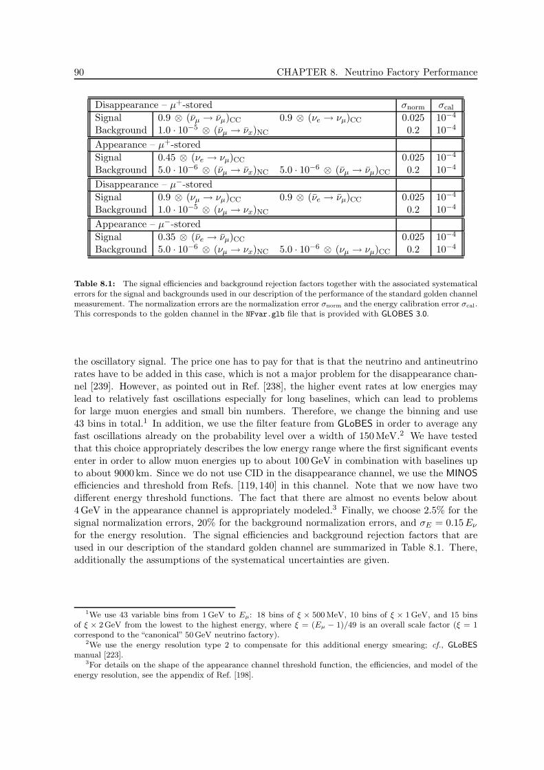
90 CHAPTER 8. Neutrino Factory Performance

Disappearance – µ+-stored σnorm σcal

Signal 0.9 ⊗ (νµ → νµ)CC 0.9 ⊗ (νe → νµ)CC 0.025 10−4

Background 1.0 · 10−5 ⊗ (νµ → νx)NC 0.2 10−4

Appearance – µ+-stored

Signal 0.45 ⊗ (νe → νµ)CC 0.025 10−4

Background 5.0 · 10−6 ⊗ (νµ → νx)NC 5.0 · 10−6 ⊗ (νµ → νµ)CC 0.2 10−4

Disappearance – µ−-stored

Signal 0.9 ⊗ (νµ → νµ)CC 0.9 ⊗ (νe → νµ)CC 0.025 10−4

Background 1.0 · 10−5 ⊗ (νµ → νx)NC 0.2 10−4

Appearance – µ−-stored

Signal 0.35 ⊗ (νe → νµ)CC 0.025 10−4

Background 5.0 · 10−6 ⊗ (νµ → νx)NC 5.0 · 10−6 ⊗ (νµ → νµ)CC 0.2 10−4

Table 8.1: The signal efficiencies and background rejection factors together with the associated systematicalerrors for the signal and backgrounds used in our description of the performance of the standard golden channelmeasurement. The normalization errors are the normalization error σnorm and the energy calibration error σcal.This corresponds to the golden channel in the NFvar.glb file that is provided with GLOBES 3.0.

the oscillatory signal. The price one has to pay for that is that the neutrino and antineutrinorates have to be added in this case, which is not a major problem for the disappearance chan-nel [239]. However, as pointed out in Ref. [238], the higher event rates at low energies maylead to relatively fast oscillations especially for long baselines, which can lead to problemsfor large muon energies and small bin numbers. Therefore, we change the binning and use43 bins in total.1 In addition, we use the filter feature from GLoBES in order to average anyfast oscillations already on the probability level over a width of 150MeV.2 We have testedthat this choice appropriately describes the low energy range where the first significant eventsenter in order to allow muon energies up to about 100GeV in combination with baselines upto about 9000 km. Since we do not use CID in the disappearance channel, we use the MINOSefficiencies and threshold from Refs. [119, 140] in this channel. Note that we now have twodifferent energy threshold functions. The fact that there are almost no events below about4GeV in the appearance channel is appropriately modeled.3 Finally, we choose 2.5% for thesignal normalization errors, 20% for the background normalization errors, and σE = 0.15Eν

for the energy resolution. The signal efficiencies and background rejection factors that areused in our description of the standard golden channel are summarized in Table 8.1. There,additionally the assumptions of the systematical uncertainties are given.

1We use 43 variable bins from 1GeV to Eµ: 18 bins of ξ × 500 MeV, 10 bins of ξ × 1GeV, and 15 binsof ξ × 2GeV from the lowest to the highest energy, where ξ = (Eµ − 1)/49 is an overall scale factor (ξ = 1correspond to the “canonical” 50GeV neutrino factory).

2We use the energy resolution type 2 to compensate for this additional energy smearing; cf., GLoBES

manual [223].3For details on the shape of the appearance channel threshold function, the efficiencies, and model of the

energy resolution, see the appendix of Ref. [198].

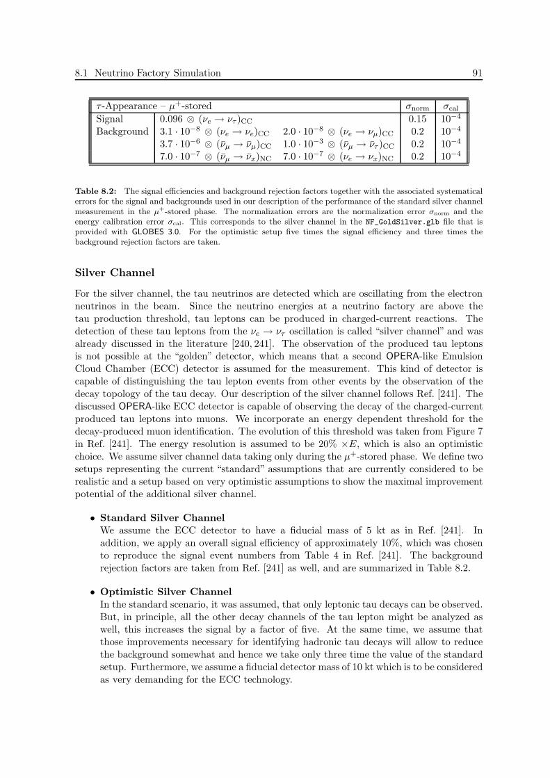
8.1 Neutrino Factory Simulation 91

τ -Appearance – µ+-stored σnorm σcal

Signal 0.096 ⊗ (νe → ντ )CC 0.15 10−4

Background 3.1 · 10−8 ⊗ (νe → νe)CC 2.0 · 10−8 ⊗ (νe → νµ)CC 0.2 10−4

3.7 · 10−6 ⊗ (νµ → νµ)CC 1.0 · 10−3 ⊗ (νµ → ντ )CC 0.2 10−4

7.0 · 10−7 ⊗ (νµ → νx)NC 7.0 · 10−7 ⊗ (νe → νx)NC 0.2 10−4

Table 8.2: The signal efficiencies and background rejection factors together with the associated systematicalerrors for the signal and backgrounds used in our description of the performance of the standard silver channelmeasurement in the µ+-stored phase. The normalization errors are the normalization error σnorm and theenergy calibration error σcal. This corresponds to the silver channel in the NF_GoldSilver.glb file that isprovided with GLOBES 3.0. For the optimistic setup five times the signal efficiency and three times thebackground rejection factors are taken.

Silver Channel

For the silver channel, the tau neutrinos are detected which are oscillating from the electronneutrinos in the beam. Since the neutrino energies at a neutrino factory are above thetau production threshold, tau leptons can be produced in charged-current reactions. Thedetection of these tau leptons from the νe → ντ oscillation is called “silver channel” and wasalready discussed in the literature [240, 241]. The observation of the produced tau leptonsis not possible at the “golden” detector, which means that a second OPERA-like EmulsionCloud Chamber (ECC) detector is assumed for the measurement. This kind of detector iscapable of distinguishing the tau lepton events from other events by the observation of thedecay topology of the tau decay. Our description of the silver channel follows Ref. [241]. Thediscussed OPERA-like ECC detector is capable of observing the decay of the charged-currentproduced tau leptons into muons. We incorporate an energy dependent threshold for thedecay-produced muon identification. The evolution of this threshold was taken from Figure 7in Ref. [241]. The energy resolution is assumed to be 20% ×E, which is also an optimisticchoice. We assume silver channel data taking only during the µ+-stored phase. We define twosetups representing the current “standard” assumptions that are currently considered to berealistic and a setup based on very optimistic assumptions to show the maximal improvementpotential of the additional silver channel.

• Standard Silver ChannelWe assume the ECC detector to have a fiducial mass of 5 kt as in Ref. [241]. Inaddition, we apply an overall signal efficiency of approximately 10%, which was chosento reproduce the signal event numbers from Table 4 in Ref. [241]. The backgroundrejection factors are taken from Ref. [241] as well, and are summarized in Table 8.2.

• Optimistic Silver ChannelIn the standard scenario, it was assumed, that only leptonic tau decays can be observed.But, in principle, all the other decay channels of the tau lepton might be analyzed aswell, this increases the signal by a factor of five. At the same time, we assume thatthose improvements necessary for identifying hadronic tau decays will allow to reducethe background somewhat and hence we take only three time the value of the standardsetup. Furthermore, we assume a fiducial detector mass of 10 kt which is to be consideredas very demanding for the ECC technology.

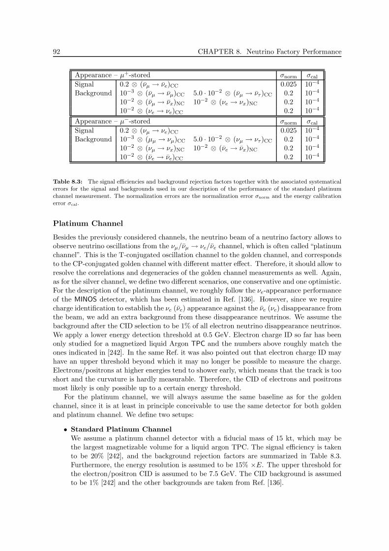
92 CHAPTER 8. Neutrino Factory Performance

Appearance – µ+-stored σnorm σcal

Signal 0.2 ⊗ (νµ → νe)CC 0.025 10−4

Background 10−3 ⊗ (νµ → νµ)CC 5.0 · 10−2 ⊗ (νµ → ντ )CC 0.2 10−4

10−2 ⊗ (νµ → νx)NC 10−2 ⊗ (νe → νx)NC 0.2 10−4

10−2 ⊗ (νe → νe)CC 0.2 10−4

Appearance – µ−-stored σnorm σcal

Signal 0.2 ⊗ (νµ → νe)CC 0.025 10−4

Background 10−3 ⊗ (µµ → νµ)CC 5.0 · 10−2 ⊗ (νµ → ντ )CC 0.2 10−4

10−2 ⊗ (νµ → νx)NC 10−2 ⊗ (νe → νx)NC 0.2 10−4

10−2 ⊗ (νe → νe)CC 0.2 10−4

Table 8.3: The signal efficiencies and background rejection factors together with the associated systematicalerrors for the signal and backgrounds used in our description of the performance of the standard platinumchannel measurement. The normalization errors are the normalization error σnorm and the energy calibrationerror σcal.

Platinum Channel

Besides the previously considered channels, the neutrino beam of a neutrino factory allows toobserve neutrino oscillations from the νµ/νµ → νe/νe channel, which is often called “platinumchannel”. This is the T-conjugated oscillation channel to the golden channel, and correspondsto the CP-conjugated golden channel with different matter effect. Therefore, it should allow toresolve the correlations and degeneracies of the golden channel measurements as well. Again,as for the silver channel, we define two different scenarios, one conservative and one optimistic.For the description of the platinum channel, we roughly follow the νe-appearance performanceof the MINOS detector, which has been estimated in Ref. [136]. However, since we requirecharge identification to establish the νe (νe) appearance against the νe (νe) disappearance fromthe beam, we add an extra background from these disappearance neutrinos. We assume thebackground after the CID selection to be 1% of all electron neutrino disappearance neutrinos.We apply a lower energy detection threshold at 0.5 GeV. Electron charge ID so far has beenonly studied for a magnetized liquid Argon TPC and the numbers above roughly match theones indicated in [242]. In the same Ref. it was also pointed out that electron charge ID mayhave an upper threshold beyond which it may no longer be possible to measure the charge.Electrons/positrons at higher energies tend to shower early, which means that the track is tooshort and the curvature is hardly measurable. Therefore, the CID of electrons and positronsmost likely is only possible up to a certain energy threshold.

For the platinum channel, we will always assume the same baseline as for the goldenchannel, since it is at least in principle conceivable to use the same detector for both goldenand platinum channel. We define two setups:

• Standard Platinum ChannelWe assume a platinum channel detector with a fiducial mass of 15 kt, which may bethe largest magnetizable volume for a liquid argon TPC. The signal efficiency is takento be 20% [242], and the background rejection factors are summarized in Table 8.3.Furthermore, the energy resolution is assumed to be 15% ×E. The upper threshold forthe electron/positron CID is assumed to be 7.5 GeV. The CID background is assumedto be 1% [242] and the other backgrounds are taken from Ref. [136].

8.1 Neutrino Factory Simulation 93

• Optimistic Platinum ChannelWe assume a platinum channel detector with a fiducial mass of 50 kt. This choice isinspired by the possibility (at least in principle) to use the same, improved detectorthan for the golden channel. The signal efficiency is 40%. The background rejectionfactors of Ref. [136] are extrapolated to higher energies. The CID background is thesame than for the standard setup. Electron/positron CID is assumed to be possible tothe highest energies and no upper threshold is imposed.

Hybrid Detector for the Optimized Golden Channel

The main limitation of a neutrino factory compared to other advanced neutrino facilities comesfrom the fact the standard detector has a relatively high neutrino energy threshold (necessaryfor charge identification), which makes the first oscillation maximum basically inaccessible(cf., Ref. [243]). All measurements have therefore to be performed in the high energy tail ofthe oscillation probability off the oscillation maximum. In different words, a neutrino factoryis optimized for high statistics in the appearance channel, not for operation at the oscillationmaximum. This is the reason why it seems to be the experiment most affected by the eightfolddegeneracy [41,198]. A number of solutions to this degeneracies problem has been proposed,amongst them it has been studied what a better detector in terms of a better neutrino energythreshold could achieve [198]. We will pick up this starting point and discuss improvementsin the detection threshold and energy resolution in this section.

The high neutrino energy threshold in Ref. [243] is the result from optimizing for the purestpossible sample of wrong sign muons, which clearly puts the emphasis on events with a highenergy muon. The lower the muon energy is, the higher the likelihood to misidentify the muoncharge or the nature of the event (CC vs NC) becomes. Thus the background increases withdecreasing neutrino energy, since the average muon energy will decrease with the neutrinoenergy. The background fraction scales with the neutrino energy such as a power law with aspectral index around −2. Our background model assumes that whatever happens with thethreshold will only affect events below the threshold, but not events above, i.e., there is onlydown-feeding of background but no up-feeding. The reason behind this assumption is that amis-identified NC event always should have a reconstructed energy which is lower than thetrue energy, since there is missing energy in every NC event. In order to roughly match thetotal background obtained in Ref. [243], we use a background fraction βE−2

ν with β = 10−3.Integrating this background fraction from 4GeV to 50GeV yields an average backgroundfraction of 5 · 10−6. We assume this background fraction separately for the background fromneutral currents and wrong sign muons.

Achieving a lower threshold probably requires a finer granularity of the detector, i.e., ahigher sampling density in the calorimeter. This should at the same time improve the energyresolution of the detector. We use a parameterization σE [GeV] = σ

√

Eν [GeV] + 0.085GeVwith σ = 0.15 for the energy resolution (as compared to σE = 0.15Eν before, corresponding toσ ≃ 0.5), where the constant part models a lower limit from Fermi motion.4 For definiteness,we take the neutrino energy threshold to be 1GeV, and the efficiency to be constant 0.5 forall appearance neutrino events above threshold. Similar numbers are quoted for the NOνAdetector [145], which is a totally active calorimeter5.

4For the neutrino factory, this lower limit turns out to be of secondary importance because there arepractically no events in the relevant energy range.

5Using an air coil system similar to the one in ATLAS, it should be possible to magnetize a detector like

94 CHAPTER 8. Neutrino Factory Performance

8.2 Neutrino Factory Optimization

After discussing the optimization of β-Beam experiments in greater detail in the last chapterwe will here present the corresponding discussion considering Neutrino Factory experiments.The main properties that can be arranged are the baseline L between neutrino source anddetector and secondly the associated neutrino energy that is set by the parent energy Eµ ofthe stored muons in the storage ring. The optimal settings are to be explored, such that thesensitivity limit to sin2 2θ13, the sensitivity to maximal CP violation, and the sensitivity to themass hierarchy are most effectively optimized. Such an optimization was already performedin [236] for slightly different assumptions for the set of neutrino oscillation parameters. Themain focus of this section will however lie on the baseline optimization, since the analysisin [236] showed that tuning the neutrino energy by Eµ does not lead to significant improvementof the respective sensitivities beyond parent muon energies Eµ & 20 − 30 GeV. The widelydiscussed standard value is Eµ = 50 GeV, however a lower parent muon energy could be aneffective tool to reduce the costs of the complete project and hence is also very worthwhile tobe discussed. For the optimization of the Neutrino Factory setup we only consider the standardgolden channel.

Sensitivity to θ13

The first performance indicator that will be discussed is the sensitivity limit to sin2 2θ13 asa function of the baseline. The range of the baseline is modified between L = 500 km andL = 10000 km, so that also the magic baseline at L ∼7500 km is covered. Note, that even thelargest discussed baseline of L = 10000 km still does not strike the outer core of the earth thatstarts approximately in a depth of 3000 km and so the neutrinos still only travel through theearth’s mantle. The final sensitivity is strongly affected by systematical uncertainties and evenmore by the parameter correlations and degeneracies as can be seen from Fig. 8.1. As in thecorresponding discussion for the β-Beam in the last chapter, these effects are indicated by thebands. The dark grey/blue band displays the impact of the systematical uncertainties to thepure statistical limit that is given by the lowermost curve. Effects of correlations are indicatedby the medium grey/blue band and finally if also the degeneracies are considered, the brightgrey/blue band gives the modification to the final sensitivity limit that is given by the thickblack curve. The left plot of Fig. 8.1 is for a low energy Neutrino Factory scenario with a parentmuon energy Eµ = 25 GeV and the right plot is for a standard scenario with Eµ = 50 GeV.It was checked, that an even higher energy Neutrino Factory scenario with Eµ = 80 GeV givesa very similar evolution of the final sensitivity limit compared to the Eµ = 50 GeV scenario.The best statistical sensitivity to θ13 is achieved for smaller baselines at L ∼ 2000 km forEµ = 25 GeV and L ∼ 3000 − 4000 km for the Eµ = 50 GeV scenario. A further outcomeis, that the effect of the systematical uncertainties is small compared to the effect of theparameter correlations and the degeneracies. These can spoil the final sensitivity limit bymore than two orders of magnitude in sin2 2θ13 compared to the systematics only limit. Forboth considered parent muon energies the magic baseline and its effect is clearly visible atL ∼7500 km where the final limit can be pushed almost down to sin2 2θ13 ∼ 10−4. The lowenergy scenario achieves the unambiguously best sensitivity to θ13 at the magic baseline. Forthe higher energy scenario with Eµ = 50 GeV there exists a second baseline range, where aclearly better sensitivity can be obtained at L ∼ 4000 km. In this small energy range the

this.

8.2 Neutrino Factory Optimization 95

2000 4000 6000 8000 10000L @kmD

10-6

10-5

10-4

10-3

10-2

10-1

Sen

sitiv

itylim

itto

sin2

2Θ13

NF - EΜ =25GeV

3Σ

GLoBES 3.0 H2007L

Systematics

Correlations

Degeneracies

2000 4000 6000 8000 10000L @kmD

10-6

10-5

10-4

10-3

10-2

10-1

Sen

sitiv

itylim

itto

sin2

2Θ13

2000 4000 6000 8000 10000L @kmD

10-6

10-5

10-4

10-3

10-2

10-1

Sen

sitiv

itylim

itto

sin2

2Θ13

NF - EΜ =50GeV

3Σ

GLoBES 3.0 H2007L

Systematics

Correlations

Degeneracies

4Σ

2000 4000 6000 8000 10000L @kmD

10-6

10-5

10-4

10-3

10-2

10-1

Sen

sitiv

itylim

itto

sin2

2Θ13

Figure 8.1: The sensitivity limit to sin2 2θ13 at a Neutrino Factory at the 3σ confidence level as a functionof the baseline L for a fixed parent muon energy Eµ = 25 GeV (left) and Eµ = 50 GeV (right). The bandsindicate the influence of systematics, correlations, and degeneracies and the final sensitivity limit is indicatedby the uppermost thick black line. In the right plot the degeneracies can be resolved around a baseline of4000 km at 3σ and the sensitivity limit to sin2 2θ13 improves by one order of magnitude. However, already atthe 4σ confidence level the degeneracies cannot be resolved anymore as indicated by the grey line.

degeneracies can be resolved. This can be understood as the following. In the baseline range1000 km . L . 6000 km the effect of the correlations drops by one order of magnitude becausein this range the local minimum in the ∆χ2 distribution at higher fit values of sin2 2θ13 dueto the (sin2 2θ13, δCP)-degeneracy gets disconnected from the true solution (global minimumat a fit value of sin2 2θ13 = 0 as there the true value is set) at the considered confidence levelof 3σ. For baselines L ∼ 4000 km and Eµ = 50 GeV this local minimum is shifted above∆χ2 = 9 and hence can be excluded. However this exclusion is not very robust and alreadyat a chosen confidence level of 4σ the resolution of the (sin2 2θ13, δCP)-degeneracy disappearsas is indicated by the thick grey line in the right plot of Fig. 8.1 that indicates the evolutionof the final sensitivity limit at 4σ. So, it is obvious that the L ∼ 4000 km Neutrino Factory isnot as extremely unique as could be concluded from the evolution of the sensitivity at 3σ. Itis worthwhile to mention that the huge impact of switching on the parameter degeneracies atthese baselines is almost only due to the (sin2 2θ13, δCP)-degeneracy while the small impact ofparameter degeneracies at the magic baseline is solely caused by the sign-degeneracy as theparameter δCP does not enter the appearance probability at this baseline.

In Fig. 8.2 the parent muon energy dependency of the sensitivity limit to sin2 2θ13 isillustrated for the fixed baselines L = 4000 km (left plot) and L = 7500 km (right plot)that were the two most promising baselines in the previous discussion. It was mentionedbefore, that lower parent muon energies could be a very interesting option since directlyconnected to the cost effort that has to be expended. We observe that the ability to excludethe (sin2 2θ13, δCP)-degeneracy at the 3σ confidence level that was already found in case ofEµ = 50 GeV is already present for parent muon energies Eµ > 30 GeV and for even higherenergies there cannot be deduced any significant improvement in the final sensitivity limit tosin2 2θ13 although the statistical limit still sees some kind of improvement due to the higher

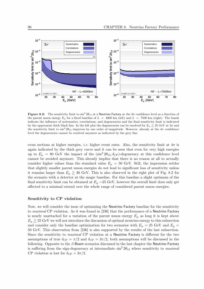
96 CHAPTER 8. Neutrino Factory Performance

20 30 40 50 60 70 80EΜ @GeVD

10-6

10-5

10-4

10-3

10-2

10-1

Sen

sitiv

itylim

itto

sin2

2Θ13

NF - L=4000km

3Σ

GLoBES 3.0 H2007L

Systematics

Correlations

Degeneracies

4Σ

20 30 40 50 60 70 80EΜ @GeVD

10-6

10-5

10-4

10-3

10-2

10-1

Sen

sitiv

itylim

itto

sin2

2Θ13

20 30 40 50 60 70 80EΜ @GeVD

10-6

10-5

10-4

10-3

10-2

10-1

Sen

sitiv

itylim

itto

sin2

2Θ13

NF - L=7500km

3Σ

GLoBES 3.0 H2007L

Systematics

Correlations

Degeneracies

20 30 40 50 60 70 80EΜ @GeVD

10-6

10-5

10-4

10-3

10-2

10-1

Sen

sitiv

itylim

itto

sin2

2Θ13

Figure 8.2: The sensitivity limit to sin2 2θ13 at a Neutrino Factory at the 3σ confidence level as a function ofthe parent muon energy Eµ for a fixed baseline of L = 4000 km (left) and L = 7500 km (right). The bandsindicate the influence of systematics, correlations, and degeneracies and the final sensitivity limit is indicatedby the uppermost thick black line. In the left plot the degeneracies can be resolved for Eµ & 25 GeV at 3σ andthe sensitivity limit to sin2 2θ13 improves by one order of magnitude. However, already at the 4σ confidencelevel the degeneracies cannot be resolved anymore as indicated by the grey line.

cross sections at higher energies, i.e. higher event rates. Also, the sensitivity limit at 4σ isagain indicated by the thick grey curve and it can be seen that even for very high energiesup to Eµ = 80 GeV the impact of the (sin2 2θ13, δCP)-degeneracy at this confidence levelcannot be avoided anymore. This already implies that there is no reason at all to actuallyconsider higher values than the standard value Eµ = 50 GeV. Still, the impression settlesthat slightly smaller parent muon energies do not lead to significant loss of sensitivity unlessit remains larger than Eµ & 30 GeV. This is also observed in the right plot of Fig. 8.2 forthe scenario with a detector at the magic baseline. For this baseline a slight optimum of thefinal sensitivity limit can be obtained at Eµ ∼25 GeV, however the overall limit does only getaffected to a minimal extend over the whole range of considered parent muon energies.

Sensitivity to CP violation

Now, we will consider the issue of optimizing the Neutrino Factory baseline for the sensitivityto maximal CP violation. As it was found in [236] that the performance of a Neutrino Factoryis nearly unattached for a variation of the parent muon energy Eµ as long it is kept aboveEµ & 25 GeV we will not introduce the discussion of optimal neutrino energy to this subsectionand consider only the baseline optimization for two scenarios with Eµ = 25 GeV and Eµ =50 GeV. This observation from [236] is also supported by the results of the last subsection.Since the sensitivity to maximal CP violation at a Neutrino Factory is different for the twoassumptions of true δCP = π/2 and δCP = 3π/2, both assumptions will be discussed in thefollowing. Opposite to the β-Beam scenarios discussed in the last chapter the Neutrino Factoryis suffering from the sign-degeneracy at intermediate sin2 2θ13 where sensitivity to maximalCP violation is lost for δCP = 3π/2.

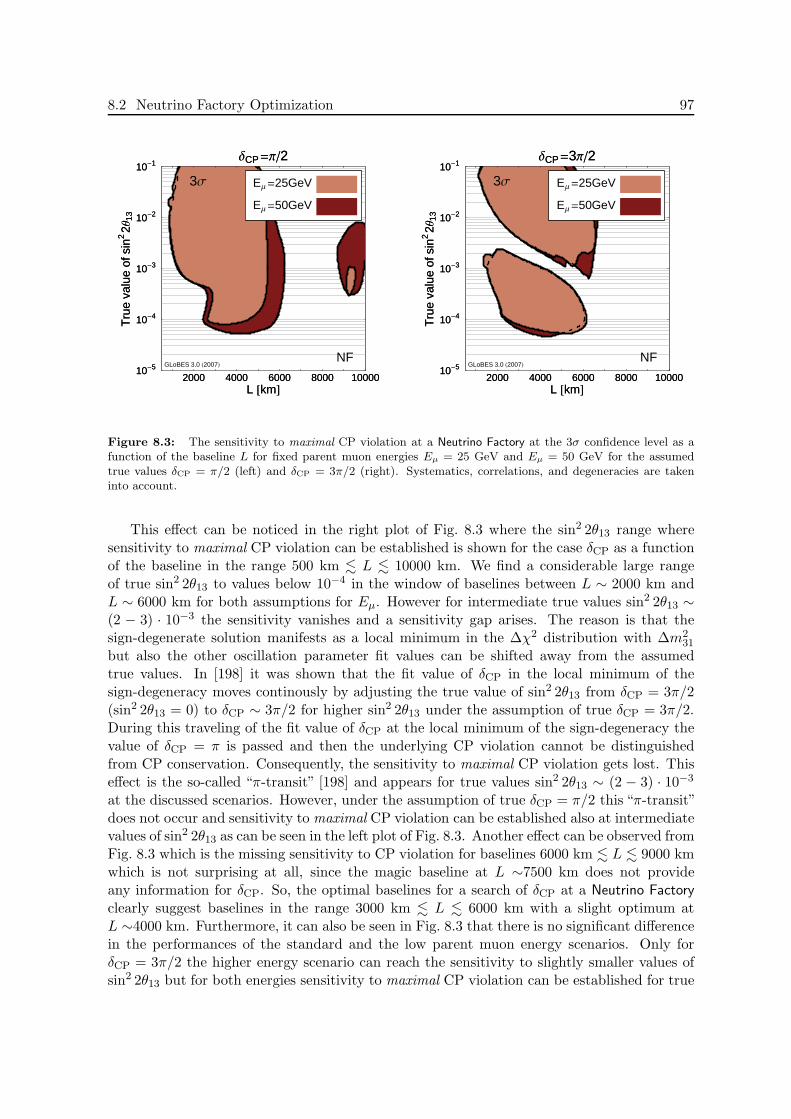
8.2 Neutrino Factory Optimization 97

2000 4000 6000 8000 10000L @kmD

10-5

10-4

10-3

10-2

10-1

Tru

eva

lue

ofsi

n22Θ

13

∆CP =Π2

NFGLoBES 3.0 H2007L

EΜ =25GeV

EΜ =50GeV

3Σ

2000 4000 6000 8000 10000L @kmD

10-5

10-4

10-3

10-2

10-1

Tru

eva

lue

ofsi

n22Θ

13

∆CP =Π2

2000 4000 6000 8000 10000L @kmD

10-5

10-4

10-3

10-2

10-1

Tru

eva

lue

ofsi

n22Θ

13

∆CP =3Π2

NFGLoBES 3.0 H2007L

EΜ =25GeV

EΜ =50GeV

3Σ

2000 4000 6000 8000 10000L @kmD

10-5

10-4

10-3

10-2

10-1

Tru

eva

lue

ofsi

n22Θ

13

∆CP =3Π2

Figure 8.3: The sensitivity to maximal CP violation at a Neutrino Factory at the 3σ confidence level as afunction of the baseline L for fixed parent muon energies Eµ = 25 GeV and Eµ = 50 GeV for the assumedtrue values δCP = π/2 (left) and δCP = 3π/2 (right). Systematics, correlations, and degeneracies are takeninto account.

This effect can be noticed in the right plot of Fig. 8.3 where the sin2 2θ13 range wheresensitivity to maximal CP violation can be established is shown for the case δCP as a functionof the baseline in the range 500 km . L . 10000 km. We find a considerable large rangeof true sin2 2θ13 to values below 10−4 in the window of baselines between L ∼ 2000 km andL ∼ 6000 km for both assumptions for Eµ. However for intermediate true values sin2 2θ13 ∼(2 − 3) · 10−3 the sensitivity vanishes and a sensitivity gap arises. The reason is that thesign-degenerate solution manifests as a local minimum in the ∆χ2 distribution with ∆m2

31

but also the other oscillation parameter fit values can be shifted away from the assumedtrue values. In [198] it was shown that the fit value of δCP in the local minimum of thesign-degeneracy moves continously by adjusting the true value of sin2 2θ13 from δCP = 3π/2(sin2 2θ13 = 0) to δCP ∼ 3π/2 for higher sin2 2θ13 under the assumption of true δCP = 3π/2.During this traveling of the fit value of δCP at the local minimum of the sign-degeneracy thevalue of δCP = π is passed and then the underlying CP violation cannot be distinguishedfrom CP conservation. Consequently, the sensitivity to maximal CP violation gets lost. Thiseffect is the so-called “π-transit” [198] and appears for true values sin2 2θ13 ∼ (2 − 3) · 10−3

at the discussed scenarios. However, under the assumption of true δCP = π/2 this “π-transit”does not occur and sensitivity to maximal CP violation can be established also at intermediatevalues of sin2 2θ13 as can be seen in the left plot of Fig. 8.3. Another effect can be observed fromFig. 8.3 which is the missing sensitivity to CP violation for baselines 6000 km . L . 9000 kmwhich is not surprising at all, since the magic baseline at L ∼7500 km does not provideany information for δCP. So, the optimal baselines for a search of δCP at a Neutrino Factoryclearly suggest baselines in the range 3000 km . L . 6000 km with a slight optimum atL ∼4000 km. Furthermore, it can also be seen in Fig. 8.3 that there is no significant differencein the performances of the standard and the low parent muon energy scenarios. Only forδCP = 3π/2 the higher energy scenario can reach the sensitivity to slightly smaller values ofsin2 2θ13 but for both energies sensitivity to maximal CP violation can be established for true

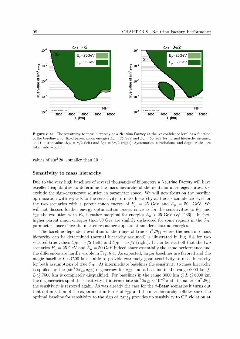
98 CHAPTER 8. Neutrino Factory Performance

2000 4000 6000 8000 10000L @kmD

10-5

10-4

10-3

10-2

10-1

Tru

eva

lue

ofsi

n22Θ

13

∆CP =Π2

NFGLoBES 3.0 H2007L

EΜ =25GeV

EΜ =50GeV

3Σ

2000 4000 6000 8000 10000L @kmD

10-5

10-4

10-3

10-2

10-1

Tru

eva

lue

ofsi

n22Θ

13

∆CP =Π2

2000 4000 6000 8000 10000L @kmD

10-5

10-4

10-3

10-2

10-1

Tru

eva

lue

ofsi

n22Θ

13

∆CP =3Π2

NFGLoBES 3.0 H2007L

EΜ =25GeV

EΜ =50GeV3Σ

2000 4000 6000 8000 10000L @kmD

10-5

10-4

10-3

10-2

10-1

Tru

eva

lue

ofsi

n22Θ

13

∆CP =3Π2

Figure 8.4: The sensitivity to mass hierarchy at a Neutrino Factory at the 3σ confidence level as a functionof the baseline L for fixed parent muon energies Eµ = 25 GeV and Eµ = 50 GeV for normal hierarchy assumedand the true values δCP = π/2 (left) and δCP = 3π/2 (right). Systematics, correlations, and degeneracies aretaken into account.

values of sin2 2θ13 smaller than 10−4.

Sensitivity to mass hierarchy

Due to the very high baselines of several thousands of kilometers a Neutrino Factory will haveexcellent capabilities to determine the mass hierarchy of the neutrino mass eigenstates, i.e.exclude the sign-degenerate solution in parameter space. We will now focus on the baselineoptimization with regards to the sensitivity to mass hierarchy at the 3σ confidence level forthe two scenarios with a parent muon energy of Eµ = 25 GeV and Eµ = 50 GeV. Wewill not discuss further energy optimization issues, since as for the sensitivities to θ13 andδCP the evolution with Eµ is rather marginal for energies Eµ > 25 GeV (cf. [236]). In fact,higher parent muon energies than 50 Gev are slightly disfavored for some regions in the δCP

parameter space since the matter resonance appears at smaller neutrino energies.

The baseline dependent evolution of the range of true sin2 2θ13 where the neutrino masshierarchy can be determined (normal hierarchy assumed) is illustrated in Fig. 8.4 for twoselected true values δCP = π/2 (left) and δCP = 3π/2 (right). It can be read off that the twoscenarios Eµ = 25 GeV and Eµ = 50 GeV indeed share essentially the same performance andthe differences are hardly visible in Fig. 8.4. As expected, larger baselines are favored and themagic baseline L ∼7500 km is able to provide extremely good sensitivity to mass hierarchyfor both assumptions of true δCP. At intermediate baselines the sensitivity to mass hierarchyis spoiled by the (sin2 2θ13, δCP)-degeneracy for δCP and a baseline in the range 6000 km .

L . 7500 km is completely disqualified. For baselines in the range 3000 km . L . 6000 kmthe degeneracies spoil the sensitivity at intermediate sin2 2θ13 ∼ 10−3 and at smaller sin2 2θ13

the sensitivity is restored again. As was already the case for the β-Beam scenarios it turns outthat optimization of the experiment in terms of δCP and the mass hierarchy collides since theoptimal baseline for sensitivity to the sign of ∆m2

31 provides no sensitivity to CP violation at

8.2 Neutrino Factory Optimization 99

all. However a baseline of L ∼4000 km seems to offer a good compromise however the resolvingof the degeneracies at intermediate sin2 2θ13 is the challenge that has to be addressed. Forthat reason we will in the following also discuss performances of Neutrino Factory scenarioswith more than one detector involved.

Neutrino Factory Reference Scenarios

The last subsections focused on the independent optimization of different Neutrino Factoryscenarios in terms of baseline L and the energy of the parent muons in the storage ringEµ. We will now assign defined reference setups, as was already done in the last chapterfor β-Beams. These follow the suggestions from the optimization discussions and provide thepossibility to study the properties and performances in a greater detail. Furthermore, thesedefined reference setups and their abilities can be comfortably compared to the performanceof the β-Beam reference setups and to each other. The definition of the reference setups isbased slightly more upon the discussion of the baseline optimization since the dependence ofthe performance on the variation of the energy turned out to be of secondary importance.So, we will stick to the standard choice Eµ = 50 GeV and only introduce one low energyscenario with Eµ = 30 GeV to further investigate if a lower energy Neutrino Factory can bejustified. Additionally, we will also introduce scenarios that involve two or even three detectorspartially located at different baselines to cover optimal performances in all three performanceindicators: discovery reach of sin2 2θ13, sensitivity to any CP violation, and sensitivity tomass hierarchy.

The standard Neutrino Factory scenario with Eµ = 50 GeV at a baseline of L = 4000 kmwill be labeled NF50@4000km. It makes use of a 50 kt Magnetized Iron detector to allow for thecharge identification of the detected muons to separate the wrong-sign muons. NF30@4000kmis basically the same setup as NF50@4000km however run at a lower energy Eµ = 30 GeVof the stored parent muons. The single detector scenario at Eµ = 50 GeV with the 50 ktMagnetized Iron detector located at L = 7500 km, i.e. approximately at the magic baseline isintroduced as NF50@7500km. Furthermore, we introduce double detector scenarios to allowfor an improved potential in degeneracy resolving. Since we are interested in the improve-ment of these double detector scenarios that is not only governed by the increased statisticsdue to the second detector, we additionally introduce a scenario that involves just a simpledoubled detector. This scenario is essentially identically to NF50@4000km with an increaseddetector volume of 100 kt and it is labeled NF50@2D1L. The next simplest double detectorscenario involves two 50 kt Magnetized Iron detectors, one located at L = 4000 km and theother at the magic baseline L = 7500 km. Since the problems of degeneracy resolving ata Neutrino Factory result from the high energy threshold due to the muon momentum cutwe also introduce a hybrid detector scenario NF50@2DlT that shows the same high energybehavior than the usually discussed detector, but with a lower energy threshold and a higherenergy resolution. The lower threshold should make the first oscillation maximum accessibleand allow for better handling of the parameter degeneracies6. Another possibility to improvethe abilities of resolving the degeneracies could be provided by the inclusion of additionalchannels that require different detector technologies. The silver channel is included for thescenario NF50@2DGS by the addition of a 10 kt Emulsion Cloud Chamber detector of theOPERA type at the same baseline L = 4000 km as the Magnetized Iron detector that allows

6In [236] it was found that the better performance of this scenario is mainly caused by the lower energythreshold and only on a secondary basis by the higher energy resolution.

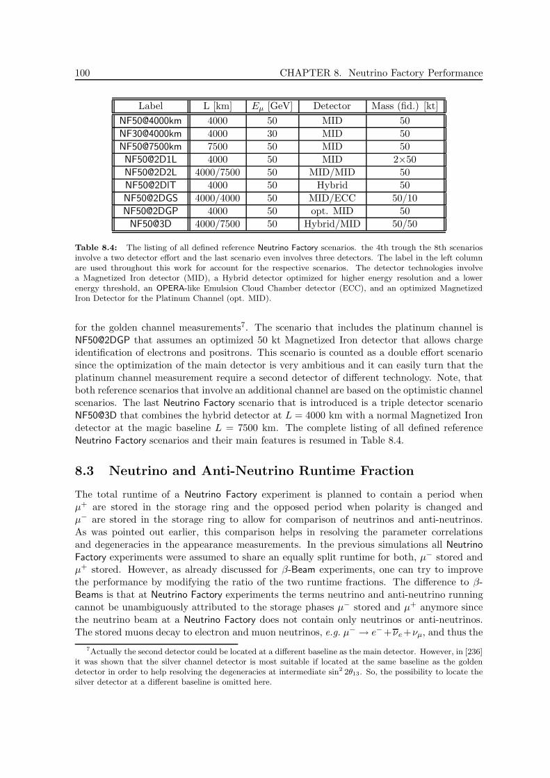
100 CHAPTER 8. Neutrino Factory Performance

Label L [km] Eµ [GeV] Detector Mass (fid.) [kt]

NF50@4000km 4000 50 MID 50

NF30@4000km 4000 30 MID 50

NF50@7500km 7500 50 MID 50

NF50@2D1L 4000 50 MID 2×50

NF50@2D2L 4000/7500 50 MID/MID 50

NF50@2DlT 4000 50 Hybrid 50

NF50@2DGS 4000/4000 50 MID/ECC 50/10

NF50@2DGP 4000 50 opt. MID 50

NF50@3D 4000/7500 50 Hybrid/MID 50/50

Table 8.4: The listing of all defined reference Neutrino Factory scenarios. the 4th trough the 8th scenariosinvolve a two detector effort and the last scenario even involves three detectors. The label in the left columnare used throughout this work for account for the respective scenarios. The detector technologies involvea Magnetized Iron detector (MID), a Hybrid detector optimized for higher energy resolution and a lowerenergy threshold, an OPERA-like Emulsion Cloud Chamber detector (ECC), and an optimized MagnetizedIron Detector for the Platinum Channel (opt. MID).

for the golden channel measurements7. The scenario that includes the platinum channel isNF50@2DGP that assumes an optimized 50 kt Magnetized Iron detector that allows chargeidentification of electrons and positrons. This scenario is counted as a double effort scenariosince the optimization of the main detector is very ambitious and it can easily turn that theplatinum channel measurement require a second detector of different technology. Note, thatboth reference scenarios that involve an additional channel are based on the optimistic channelscenarios. The last Neutrino Factory scenario that is introduced is a triple detector scenarioNF50@3D that combines the hybrid detector at L = 4000 km with a normal Magnetized Irondetector at the magic baseline L = 7500 km. The complete listing of all defined referenceNeutrino Factory scenarios and their main features is resumed in Table 8.4.

8.3 Neutrino and Anti-Neutrino Runtime Fraction

The total runtime of a Neutrino Factory experiment is planned to contain a period whenµ+ are stored in the storage ring and the opposed period when polarity is changed andµ− are stored in the storage ring to allow for comparison of neutrinos and anti-neutrinos.As was pointed out earlier, this comparison helps in resolving the parameter correlationsand degeneracies in the appearance measurements. In the previous simulations all NeutrinoFactory experiments were assumed to share an equally split runtime for both, µ− stored andµ+ stored. However, as already discussed for β-Beam experiments, one can try to improvethe performance by modifying the ratio of the two runtime fractions. The difference to β-Beams is that at Neutrino Factory experiments the terms neutrino and anti-neutrino runningcannot be unambiguously attributed to the storage phases µ− stored and µ+ anymore sincethe neutrino beam at a Neutrino Factory does not contain only neutrinos or anti-neutrinos.The stored muons decay to electron and muon neutrinos, e.g. µ− → e−+νe +νµ, and thus the

7Actually the second detector could be located at a different baseline as the main detector. However, in [236]it was shown that the silver channel detector is most suitable if located at the same baseline as the goldendetector in order to help resolving the degeneracies at intermediate sin2 2θ13. So, the possibility to locate thesilver detector at a different baseline is omitted here.

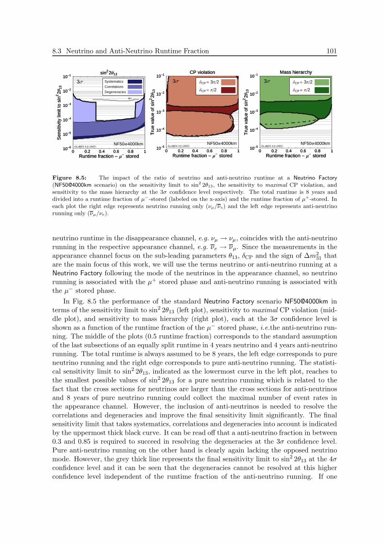
8.3 Neutrino and Anti-Neutrino Runtime Fraction 101

0 0.2 0.4 0.6 0.8 1Runtime fraction - Μ

- stored

10-6

10-5

10-4

10-3

10-2

10-1

Sen

sitiv

itylim

itto

sin2

2Θ13

sin22Θ13

NF504000km

3Σ

GLoBES 3.0 H2007L

Systematics

Correlations

Degeneracies

4Σ

0 0.2 0.4 0.6 0.8 1Runtime fraction - Μ

- stored

10-6

10-5

10-4

10-3

10-2

10-1

Sen

sitiv

itylim

itto

sin2

2Θ13

sin22Θ13

0 0.2 0.4 0.6 0.8 1Runtime fraction - Μ

- stored

10-5

10-4

10-3

10-2

10-1

Tru

eva

lue

ofsi

n22Θ

13

CP violation

NF504000kmGLoBES 3.0 H2007L

∆CP = 3Π2

∆CP = Π2

3Σ

0 0.2 0.4 0.6 0.8 1Runtime fraction - Μ

- stored

10-5

10-4

10-3

10-2

10-1

Tru

eva

lue

ofsi

n22Θ

13

CP violation

0 0.2 0.4 0.6 0.8 1Runtime fraction - Μ

- stored

10-5

10-4

10-3

10-2

10-1

Tru

eva

lue

ofsi

n22Θ

13

Mass hierarchy

NF504000kmGLoBES 3.0 H2007L

∆CP = 3Π2

∆CP = Π2

3Σ

0 0.2 0.4 0.6 0.8 1Runtime fraction - Μ

- stored

10-5

10-4

10-3

10-2

10-1

Tru

eva

lue

ofsi

n22Θ

13

Mass hierarchy

Figure 8.5: The impact of the ratio of neutrino and anti-neutrino runtime at a Neutrino Factory

(NF50@4000km scenario) on the sensitivity limit to sin2 2θ13, the sensitivity to maximal CP violation, andsensitivity to the mass hierarchy at the 3σ confidence level respectively. The total runtime is 8 years anddivided into a runtime fraction of µ−-stored (labeled on the x-axis) and the runtime fraction of µ+-stored. Ineach plot the right edge represents neutrino running only (νµ/νe) and the left edge represents anti-neutrinorunning only (νµ/νe).

neutrino runtime in the disappearance channel, e.g. νµ → νµ, coincides with the anti-neutrinorunning in the respective appearance channel, e.g. νe → νµ. Since the measurements in theappearance channel focus on the sub-leading parameters θ13, δCP and the sign of ∆m2

31 thatare the main focus of this work, we will use the terms neutrino or anti-neutrino running at aNeutrino Factory following the mode of the neutrinos in the appearance channel, so neutrinorunning is associated with the µ+ stored phase and anti-neutrino running is associated withthe µ− stored phase.

In Fig. 8.5 the performance of the standard Neutrino Factory scenario NF50@4000km interms of the sensitivity limit to sin2 2θ13 (left plot), sensitivity to maximal CP violation (mid-dle plot), and sensitivity to mass hierarchy (right plot), each at the 3σ confidence level isshown as a function of the runtime fraction of the µ− stored phase, i.e.the anti-neutrino run-ning. The middle of the plots (0.5 runtime fraction) corresponds to the standard assumptionof the last subsections of an equally split runtime in 4 years neutrino and 4 years anti-neutrinorunning. The total runtime is always assumed to be 8 years, the left edge corresponds to pureneutrino running and the right edge corresponds to pure anti-neutrino running. The statisti-cal sensitivity limit to sin2 2θ13, indicated as the lowermost curve in the left plot, reaches tothe smallest possible values of sin2 2θ13 for a pure neutrino running which is related to thefact that the cross sections for neutrinos are larger than the cross sections for anti-neutrinosand 8 years of pure neutrino running could collect the maximal number of event rates inthe appearance channel. However, the inclusion of anti-neutrinos is needed to resolve thecorrelations and degeneracies and improve the final sensitivity limit significantly. The finalsensitivity limit that takes systematics, correlations and degeneracies into account is indicatedby the uppermost thick black curve. It can be read off that a anti-neutrino fraction in between0.3 and 0.85 is required to succeed in resolving the degeneracies at the 3σ confidence level.Pure anti-neutrino running on the other hand is clearly again lacking the opposed neutrinomode. However, the grey thick line represents the final sensitivity limit to sin2 2θ13 at the 4σconfidence level and it can be seen that the degeneracies cannot be resolved at this higherconfidence level independent of the runtime fraction of the anti-neutrino running. If one

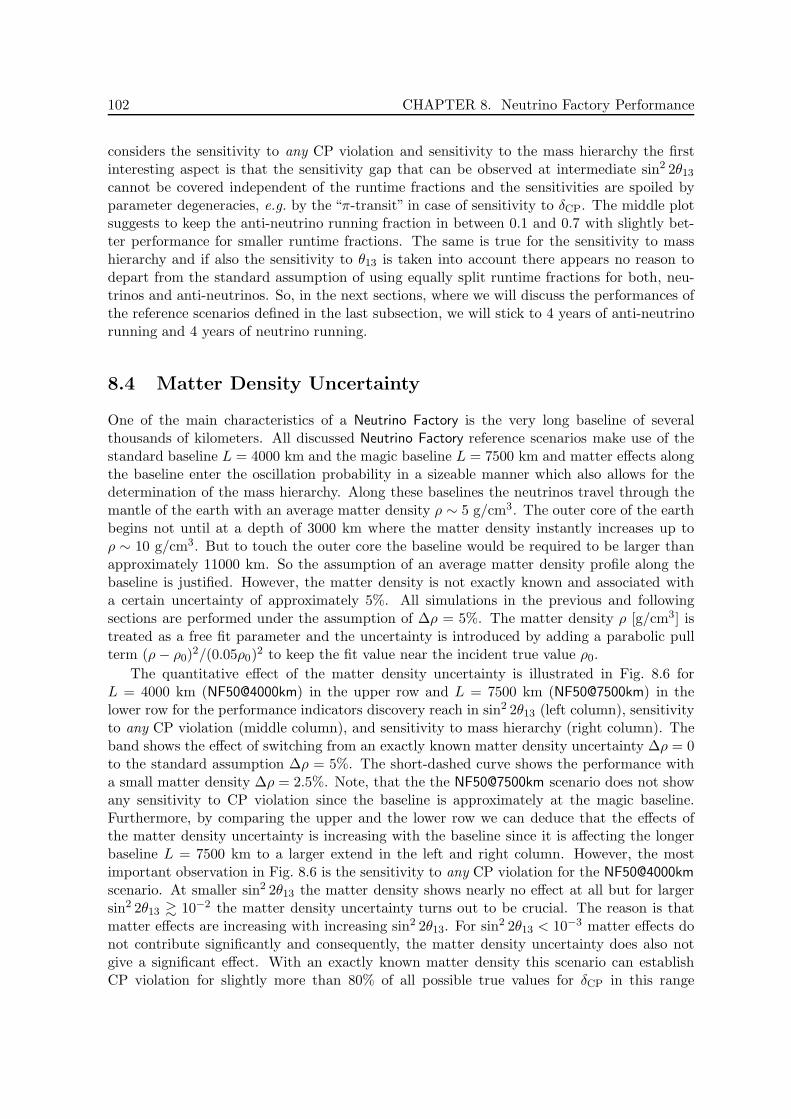
102 CHAPTER 8. Neutrino Factory Performance

considers the sensitivity to any CP violation and sensitivity to the mass hierarchy the firstinteresting aspect is that the sensitivity gap that can be observed at intermediate sin2 2θ13

cannot be covered independent of the runtime fractions and the sensitivities are spoiled byparameter degeneracies, e.g. by the “π-transit” in case of sensitivity to δCP. The middle plotsuggests to keep the anti-neutrino running fraction in between 0.1 and 0.7 with slightly bet-ter performance for smaller runtime fractions. The same is true for the sensitivity to masshierarchy and if also the sensitivity to θ13 is taken into account there appears no reason todepart from the standard assumption of using equally split runtime fractions for both, neu-trinos and anti-neutrinos. So, in the next sections, where we will discuss the performances ofthe reference scenarios defined in the last subsection, we will stick to 4 years of anti-neutrinorunning and 4 years of neutrino running.

8.4 Matter Density Uncertainty

One of the main characteristics of a Neutrino Factory is the very long baseline of severalthousands of kilometers. All discussed Neutrino Factory reference scenarios make use of thestandard baseline L = 4000 km and the magic baseline L = 7500 km and matter effects alongthe baseline enter the oscillation probability in a sizeable manner which also allows for thedetermination of the mass hierarchy. Along these baselines the neutrinos travel through themantle of the earth with an average matter density ρ ∼ 5 g/cm3. The outer core of the earthbegins not until at a depth of 3000 km where the matter density instantly increases up toρ ∼ 10 g/cm3. But to touch the outer core the baseline would be required to be larger thanapproximately 11000 km. So the assumption of an average matter density profile along thebaseline is justified. However, the matter density is not exactly known and associated witha certain uncertainty of approximately 5%. All simulations in the previous and followingsections are performed under the assumption of ∆ρ = 5%. The matter density ρ [g/cm3] istreated as a free fit parameter and the uncertainty is introduced by adding a parabolic pullterm (ρ − ρ0)

2/(0.05ρ0)2 to keep the fit value near the incident true value ρ0.

The quantitative effect of the matter density uncertainty is illustrated in Fig. 8.6 forL = 4000 km (NF50@4000km) in the upper row and L = 7500 km (NF50@7500km) in thelower row for the performance indicators discovery reach in sin2 2θ13 (left column), sensitivityto any CP violation (middle column), and sensitivity to mass hierarchy (right column). Theband shows the effect of switching from an exactly known matter density uncertainty ∆ρ = 0to the standard assumption ∆ρ = 5%. The short-dashed curve shows the performance witha small matter density ∆ρ = 2.5%. Note, that the the NF50@7500km scenario does not showany sensitivity to CP violation since the baseline is approximately at the magic baseline.Furthermore, by comparing the upper and the lower row we can deduce that the effects ofthe matter density uncertainty is increasing with the baseline since it is affecting the longerbaseline L = 7500 km to a larger extend in the left and right column. However, the mostimportant observation in Fig. 8.6 is the sensitivity to any CP violation for the NF50@4000kmscenario. At smaller sin2 2θ13 the matter density shows nearly no effect at all but for largersin2 2θ13 & 10−2 the matter density uncertainty turns out to be crucial. The reason is thatmatter effects are increasing with increasing sin2 2θ13. For sin2 2θ13 < 10−3 matter effects donot contribute significantly and consequently, the matter density uncertainty does also notgive a significant effect. With an exactly known matter density this scenario can establishCP violation for slightly more than 80% of all possible true values for δCP in this range

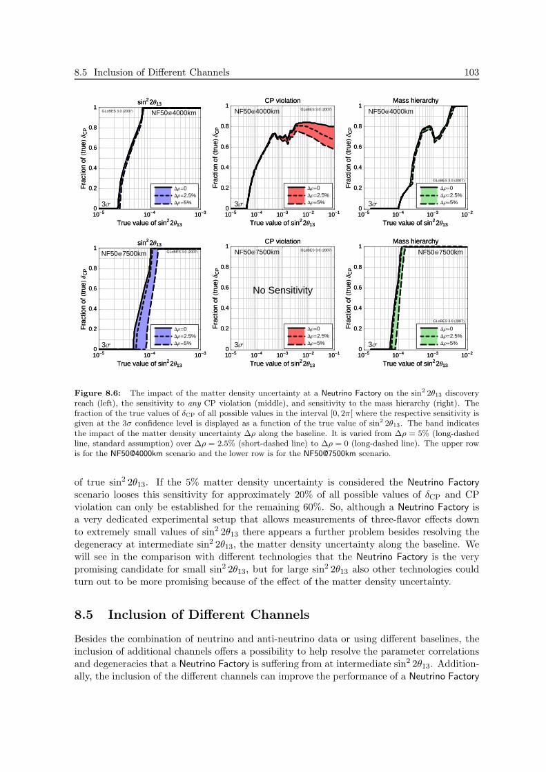
8.5 Inclusion of Different Channels 103

10-310-410-5

True value of sin22Θ13

0

0.2

0.4

0.6

0.8

1

Fra

ctio

nofHt

rueL

∆C

P

sin22Θ13

DΡ=0DΡ=2.5%DΡ=5%

GLoBES 3.0 H2007L

3Σ

NF504000km

10-310-410-5

True value of sin22Θ13

0

0.2

0.4

0.6

0.8

1

Fra

ctio

nofHt

rueL

∆C

P

sin22Θ13

10-110-210-310-410-5

True value of sin22Θ13

0

0.2

0.4

0.6

0.8

1

Fra

ctio

nofHt

rueL

∆C

P

CP violation

DΡ=0DΡ=2.5%DΡ=5%

GLoBES 3.0 H2007L

3Σ

NF504000km

10-110-210-310-410-5

True value of sin22Θ13

0

0.2

0.4

0.6

0.8

1

Fra

ctio

nofHt

rueL

∆C

P

CP violation

10-210-310-410-5

True value of sin22Θ13

0

0.2

0.4

0.6

0.8

1

Fra

ctio

nofHt

rueL

∆C

P

Mass hierarchy

DΡ=0DΡ=2.5%DΡ=5%

GLoBES 3.0 H2007L

3Σ

NF504000km

10-210-310-410-5

True value of sin22Θ13

0

0.2

0.4

0.6

0.8

1

Fra

ctio

nofHt

rueL

∆C

P

Mass hierarchy

10-310-410-5

True value of sin22Θ13

0

0.2

0.4

0.6

0.8

1

Fra

ctio

nofHt

rueL

∆C

P

sin22Θ13

DΡ=0DΡ=2.5%DΡ=5%

GLoBES 3.0 H2007L

3Σ

NF507500km

10-310-410-5

True value of sin22Θ13

0

0.2

0.4

0.6

0.8

1

Fra

ctio

nofHt

rueL

∆C

P

sin22Θ13

10-110-210-310-410-5

True value of sin22Θ13

0

0.2

0.4

0.6

0.8

1

Fra

ctio

nofHt

rueL

∆C

P

CP violation

DΡ=0DΡ=2.5%DΡ=5%

GLoBES 3.0 H2007L

3Σ

No Sensitivity

NF507500km

10-110-210-310-410-5

True value of sin22Θ13

0

0.2

0.4

0.6

0.8

1

Fra

ctio

nofHt

rueL

∆C

P

CP violation

10-210-310-410-5

True value of sin22Θ13

0

0.2

0.4

0.6

0.8

1

Fra

ctio

nofHt

rueL

∆C

P

Mass hierarchy

DΡ=0DΡ=2.5%DΡ=5%

GLoBES 3.0 H2007L

3Σ

NF507500km

10-210-310-410-5

True value of sin22Θ13

0

0.2

0.4

0.6

0.8

1

Fra

ctio

nofHt

rueL

∆C

P

Mass hierarchy

Figure 8.6: The impact of the matter density uncertainty at a Neutrino Factory on the sin2 2θ13 discoveryreach (left), the sensitivity to any CP violation (middle), and sensitivity to the mass hierarchy (right). Thefraction of the true values of δCP of all possible values in the interval [0, 2π[ where the respective sensitivity isgiven at the 3σ confidence level is displayed as a function of the true value of sin2 2θ13. The band indicatesthe impact of the matter density uncertainty ∆ρ along the baseline. It is varied from ∆ρ = 5% (long-dashedline, standard assumption) over ∆ρ = 2.5% (short-dashed line) to ∆ρ = 0 (long-dashed line). The upper rowis for the NF50@4000km scenario and the lower row is for the NF50@7500km scenario.

of true sin2 2θ13. If the 5% matter density uncertainty is considered the Neutrino Factoryscenario looses this sensitivity for approximately 20% of all possible values of δCP and CPviolation can only be established for the remaining 60%. So, although a Neutrino Factory isa very dedicated experimental setup that allows measurements of three-flavor effects downto extremely small values of sin2 2θ13 there appears a further problem besides resolving thedegeneracy at intermediate sin2 2θ13, the matter density uncertainty along the baseline. Wewill see in the comparison with different technologies that the Neutrino Factory is the verypromising candidate for small sin2 2θ13, but for large sin2 2θ13 also other technologies couldturn out to be more promising because of the effect of the matter density uncertainty.

8.5 Inclusion of Different Channels

Besides the combination of neutrino and anti-neutrino data or using different baselines, theinclusion of additional channels offers a possibility to help resolve the parameter correlationsand degeneracies that a Neutrino Factory is suffering from at intermediate sin2 2θ13. Addition-ally, the inclusion of the different channels can improve the performance of a Neutrino Factory

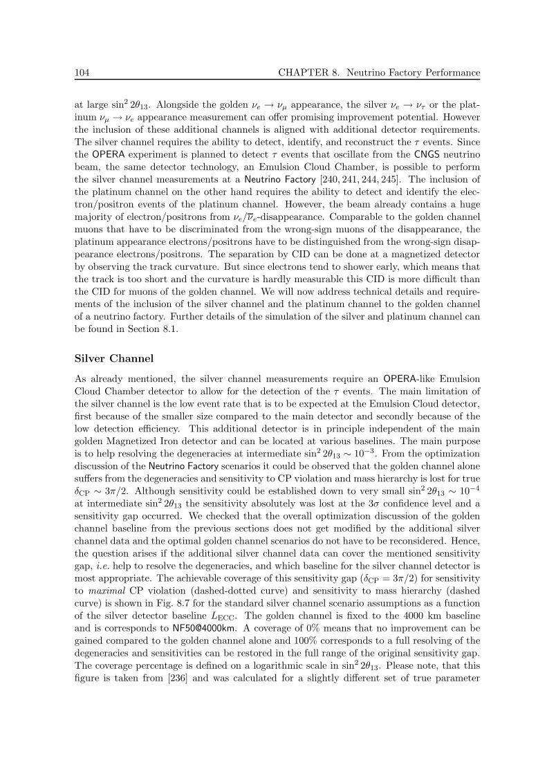
104 CHAPTER 8. Neutrino Factory Performance

at large sin2 2θ13. Alongside the golden νe → νµ appearance, the silver νe → ντ or the plat-inum νµ → νe appearance measurement can offer promising improvement potential. Howeverthe inclusion of these additional channels is aligned with additional detector requirements.The silver channel requires the ability to detect, identify, and reconstruct the τ events. Sincethe OPERA experiment is planned to detect τ events that oscillate from the CNGS neutrinobeam, the same detector technology, an Emulsion Cloud Chamber, is possible to performthe silver channel measurements at a Neutrino Factory [240, 241, 244, 245]. The inclusion ofthe platinum channel on the other hand requires the ability to detect and identify the elec-tron/positron events of the platinum channel. However, the beam already contains a hugemajority of electron/positrons from νe/νe-disappearance. Comparable to the golden channelmuons that have to be discriminated from the wrong-sign muons of the disappearance, theplatinum appearance electrons/positrons have to be distinguished from the wrong-sign disap-pearance electrons/positrons. The separation by CID can be done at a magnetized detectorby observing the track curvature. But since electrons tend to shower early, which means thatthe track is too short and the curvature is hardly measurable this CID is more difficult thanthe CID for muons of the golden channel. We will now address technical details and require-ments of the inclusion of the silver channel and the platinum channel to the golden channelof a neutrino factory. Further details of the simulation of the silver and platinum channel canbe found in Section 8.1.

Silver Channel

As already mentioned, the silver channel measurements require an OPERA-like EmulsionCloud Chamber detector to allow for the detection of the τ events. The main limitation ofthe silver channel is the low event rate that is to be expected at the Emulsion Cloud detector,first because of the smaller size compared to the main detector and secondly because of thelow detection efficiency. This additional detector is in principle independent of the maingolden Magnetized Iron detector and can be located at various baselines. The main purposeis to help resolving the degeneracies at intermediate sin2 2θ13 ∼ 10−3. From the optimizationdiscussion of the Neutrino Factory scenarios it could be observed that the golden channel alonesuffers from the degeneracies and sensitivity to CP violation and mass hierarchy is lost for trueδCP ∼ 3π/2. Although sensitivity could be established down to very small sin2 2θ13 ∼ 10−4

at intermediate sin2 2θ13 the sensitivity absolutely was lost at the 3σ confidence level and asensitivity gap occurred. We checked that the overall optimization discussion of the goldenchannel baseline from the previous sections does not get modified by the additional silverchannel data and the optimal golden channel scenarios do not have to be reconsidered. Hence,the question arises if the additional silver channel data can cover the mentioned sensitivitygap, i.e. help to resolve the degeneracies, and which baseline for the silver channel detector ismost appropriate. The achievable coverage of this sensitivity gap (δCP = 3π/2) for sensitivityto maximal CP violation (dashed-dotted curve) and sensitivity to mass hierarchy (dashedcurve) is shown in Fig. 8.7 for the standard silver channel scenario assumptions as a functionof the silver detector baseline LECC. The golden channel is fixed to the 4000 km baselineand is corresponds to NF50@4000km. A coverage of 0% means that no improvement can begained compared to the golden channel alone and 100% corresponds to a full resolving of thedegeneracies and sensitivities can be restored in the full range of the original sensitivity gap.The coverage percentage is defined on a logarithmic scale in sin2 2θ13. Please note, that thisfigure is taken from [236] and was calculated for a slightly different set of true parameter

8.5 Inclusion of Different Channels 105

2000 4000 6000 8000LECC @kmD

0

10

20

30

40

50

60

Cov

erag

eof

dege

nera

cyga

pat

3Σ@%D

Gold H50 GeV4000km fixedL + Silver

mass hierarchy

CP violation

Figure 8.7: The improvement of the degeneracy resolution potential at intermediate sin2 2θ13 by includingthe standard silver channel to the golden channel as a function of the silver channel baseline LECC. Theparent muon energy is 50 GeV and the golden channel detector is located at LMID = 4000 km. The curvesshow the coverage of the sensitivity gap at intermediate true sin2 2θ13 ∼ 10−3 for sensitivity to maximal CPviolation (dashed-dotted curve) and sensitivity to mass hierarchy (dashed curve) at the 3σ confidence level(true δCP = 3π/2 assumed). A coverage of 0% corresponds to the width of the sensitivity gap for goldenchannel only and 100% would correspond to a complete restoration of sensitivity for intermediate sin2 2θ13.The figure is taken from [236] and produced with the true parameter assumption of ∆m2

31 = 2.2 · 10−3 eV2.

values including a ∆m231 = 2.2 · 10−3 eV2. As can be read off from Fig. 8.7 the standard

silver scenario cannot resolve the degeneracies completely independent of the silver baselineand a sensitivity gap still remains for the combination of golden and silver channel data atintermediate sin2 2θ13. However, in the silver baseline range from 2000 km to 5000 km thebest performance can be observed where almost 50% of the original (golden channel only)sensitivity gap in CP violation measurements and almost 20% of the original sensitivity gapin mass hierarchy measurements can be covered by the inclusion of the silver channel data.The optimal silver baseline is approximately found at 3000 km however at 4000 km, whichis the assumed baseline of the golden detector, the performance is very similar, so we will inthe following only consider a silver detector at the same baseline as the main golden detector,since this is more cost effective because no further cavities at different baselines are required.It should be mentioned that the optimistic silver channel scenario with a doubled detectorsize and an improved signal detection can in principle cover 100% of the sensitivity gaps forboth, CP violation and mass hierarchy measurements for δCP = 3π/2. The performance ofthe optimistic silver channel will be compared to the standard scenario in the next-to-nextsubsection.

Platinum Channel

The measurement of the platinum channel is very promising since an adequately high eventrate as in the golden channel is in principle obtainable. Furthermore, this channel is the

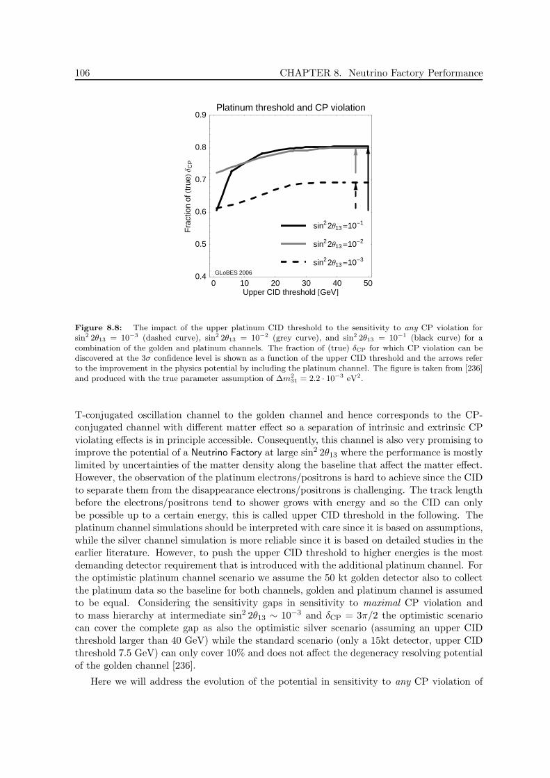
106 CHAPTER 8. Neutrino Factory Performance

0 10 20 30 40 50Upper CID threshold @GeVD

0.4

0.5

0.6

0.7

0.8

0.9

Fra

ctio

nofHt

rueL

∆C

P

Platinum threshold and CP violation

GLoBES 2006

sin22Θ13 =10-3

sin22Θ13 =10-2

sin22Θ13 =10-1

Figure 8.8: The impact of the upper platinum CID threshold to the sensitivity to any CP violation forsin2 2θ13 = 10−3 (dashed curve), sin2 2θ13 = 10−2 (grey curve), and sin2 2θ13 = 10−1 (black curve) for acombination of the golden and platinum channels. The fraction of (true) δCP for which CP violation can bediscovered at the 3σ confidence level is shown as a function of the upper CID threshold and the arrows referto the improvement in the physics potential by including the platinum channel. The figure is taken from [236]and produced with the true parameter assumption of ∆m2

31 = 2.2 · 10−3 eV2.

T-conjugated oscillation channel to the golden channel and hence corresponds to the CP-conjugated channel with different matter effect so a separation of intrinsic and extrinsic CPviolating effects is in principle accessible. Consequently, this channel is also very promising toimprove the potential of a Neutrino Factory at large sin2 2θ13 where the performance is mostlylimited by uncertainties of the matter density along the baseline that affect the matter effect.However, the observation of the platinum electrons/positrons is hard to achieve since the CIDto separate them from the disappearance electrons/positrons is challenging. The track lengthbefore the electrons/positrons tend to shower grows with energy and so the CID can onlybe possible up to a certain energy, this is called upper CID threshold in the following. Theplatinum channel simulations should be interpreted with care since it is based on assumptions,while the silver channel simulation is more reliable since it is based on detailed studies in theearlier literature. However, to push the upper CID threshold to higher energies is the mostdemanding detector requirement that is introduced with the additional platinum channel. Forthe optimistic platinum channel scenario we assume the 50 kt golden detector also to collectthe platinum data so the baseline for both channels, golden and platinum channel is assumedto be equal. Considering the sensitivity gaps in sensitivity to maximal CP violation andto mass hierarchy at intermediate sin2 2θ13 ∼ 10−3 and δCP = 3π/2 the optimistic scenariocan cover the complete gap as also the optimistic silver scenario (assuming an upper CIDthreshold larger than 40 GeV) while the standard scenario (only a 15kt detector, upper CIDthreshold 7.5 GeV) can only cover 10% and does not affect the degeneracy resolving potentialof the golden channel [236].

Here we will address the evolution of the potential in sensitivity to any CP violation of

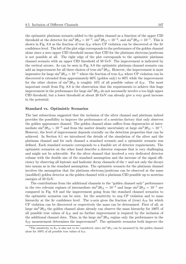
8.5 Inclusion of Different Channels 107

the optimistic platinum scenario added to the golden channel as a function of the upper CIDthreshold at the detector for sin2 2θ13 = 10−3, sin2 2θ13 = 10−2, and sin2 2θ13 = 10−1. This isshown in Fig. 8.8 as the fraction of true δCP where CP violation can be discovered at the 3σconfidence level. The left of the plot edge corresponds to the performance of the golden channelalone since a zero upper CID threshold means that CID for the platinum electrons/positronsis not possible at all. The right edge of the plot corresponds to the optimistic platinumchannel scenario with an upper CID threshold of 50 GeV. The improvement is indicated bythe vertical arrows. As can be seen in Fig. 8.8 the optimistic platinum channel scenario canadd an improvement for all three choices of true sin2 2θ13. However, the improvement is mostimpressive for large sin2 2θ13 = 10−1 where the fraction of true δCP where CP violation can bediscovered is extended from approximately 60% (golden only) to 80% while the improvementfor the other choices of sin2 2θ13 is roughly 10% of all possible values of δCP. The mostimportant result from Fig. 8.8 is the observation that the requirements to achieve this hugeimprovement in the performance for large sin2 2θ13 do not necessarily involve a too high upperCID threshold, but a lower threshold at about 20 GeV can already give a very good increasein the potential.

Standard vs. Optimistic Scenarios

The last subsections suggested that the inclusion of the silver channel and platinum indeedprovides the possibility to improve the performance of a neutrino factory that only observesthe golden appearance channel. The golden channel alone suffers from degeneracies at inter-mediate sin2 2θ13 ∼ 10−3 and from the matter density uncertainty at large sin2 2θ13 ∼ 10−1.However, the level of improvement depends crucially on the detection properties that can beachieved. In Section 8.1 we introduced the details of the simulation of the silver and theplatinum channel and for each channel a standard scenario and a optimistic scenario wasdefined. Each standard scenario corresponds to a feasible set of detector requirements. Theoptimistic scenarios on the other hand describe a detector response that is very challengingand might not be achievable. For the silver channel that involved a very dedicated detectorvolume with the double size of the standard assumption and the increase of the signal effi-ciency by observing all leptonic and hadronic decay channels of the τ and not only the decaysinto muons as in the standard assumption. The optimistic scenario for the platinum channelinvolves the assumption that the platinum electrons/positrons can be observed at the same(modified) golden detector as the golden channel with a platinum CID possible up to neutrinoenergies of 50 GeV.

The contributions from the additional channels to the “golden channel only” performancein the two relevant regimes of intermediate sin2 2θ13 = 10−3 and large sin2 2θ13 = 10−1 arecompared in Fig. 8.9 and the improvement going from the standard channel scenarios tothe optimistic scenarios can be seen. for the sensitivity to any CP violation and to masshierarchy at the 3σ confidence level. The x-axis gives the fraction of (true) δCP for whichCP violation can be discovered or respectively the mass can be determined. First of all, atlarge sin2 2θ13 the golden channel alone already can observe the mass hierarchy for 100% ofall possible true values of δCP and no further improvement is required by the inclusion ofthe additional channel data. Thus, in the large sin2 2θ13 regime only the performance in theδCP measurement determines the improvement8. The optimistic scenarios both improve the

8The sensitivity to θ13 is also not to be considered, since sin2 2θ13 can be measured by the golden channelalone for 100% of all possible true values of δCP.

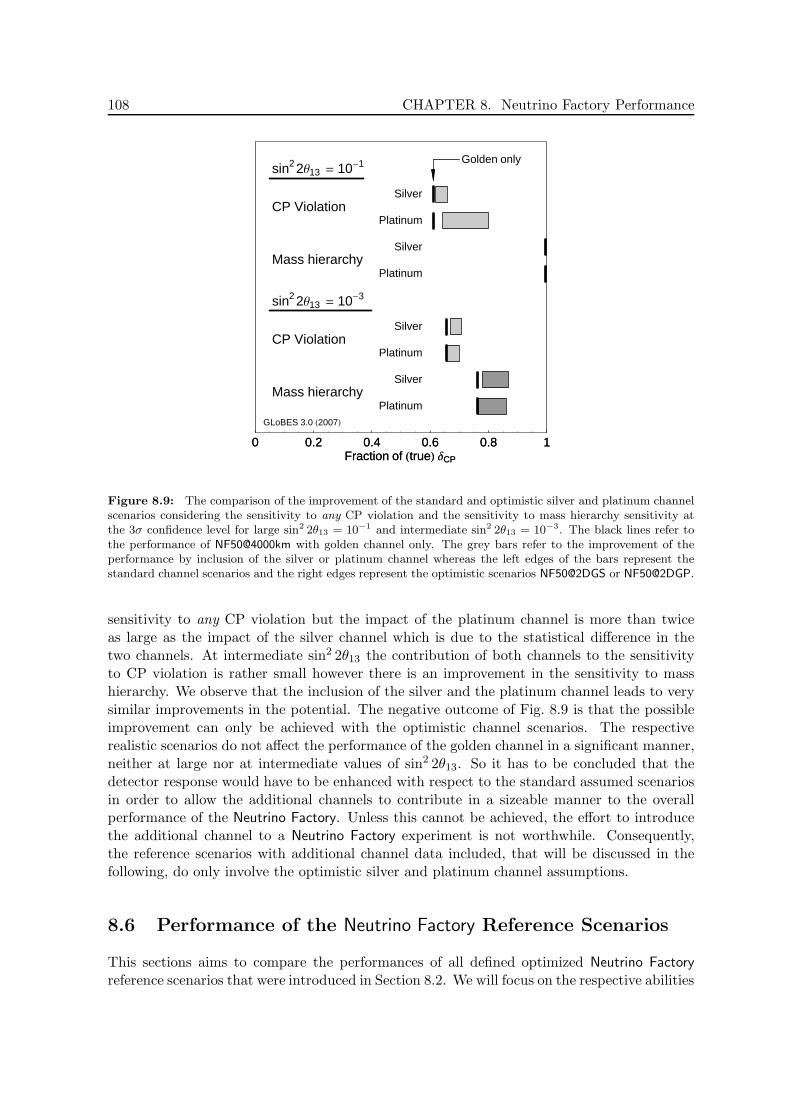
108 CHAPTER 8. Neutrino Factory Performance

0 0.2 0.4 0.6 0.8 1Fraction of HtrueL ∆CP

Silver

Silver

Silver

Silver

Platinum

Platinum

Platinum

PlatinumCP Violation

CP Violation

Mass hierarchy

Mass hierarchy

sin2 2Θ13 = 10-1

sin2 2Θ13 = 10-3

GLoBES 3.0 H2007L

Golden only

0 0.2 0.4 0.6 0.8 1Fraction of HtrueL ∆CP

Figure 8.9: The comparison of the improvement of the standard and optimistic silver and platinum channelscenarios considering the sensitivity to any CP violation and the sensitivity to mass hierarchy sensitivity atthe 3σ confidence level for large sin2 2θ13 = 10−1 and intermediate sin2 2θ13 = 10−3. The black lines refer tothe performance of NF50@4000km with golden channel only. The grey bars refer to the improvement of theperformance by inclusion of the silver or platinum channel whereas the left edges of the bars represent thestandard channel scenarios and the right edges represent the optimistic scenarios NF50@2DGS or NF50@2DGP.

sensitivity to any CP violation but the impact of the platinum channel is more than twiceas large as the impact of the silver channel which is due to the statistical difference in thetwo channels. At intermediate sin2 2θ13 the contribution of both channels to the sensitivityto CP violation is rather small however there is an improvement in the sensitivity to masshierarchy. We observe that the inclusion of the silver and the platinum channel leads to verysimilar improvements in the potential. The negative outcome of Fig. 8.9 is that the possibleimprovement can only be achieved with the optimistic channel scenarios. The respectiverealistic scenarios do not affect the performance of the golden channel in a significant manner,neither at large nor at intermediate values of sin2 2θ13. So it has to be concluded that thedetector response would have to be enhanced with respect to the standard assumed scenariosin order to allow the additional channels to contribute in a sizeable manner to the overallperformance of the Neutrino Factory. Unless this cannot be achieved, the effort to introducethe additional channel to a Neutrino Factory experiment is not worthwhile. Consequently,the reference scenarios with additional channel data included, that will be discussed in thefollowing, do only involve the optimistic silver and platinum channel assumptions.

8.6 Performance of the Neutrino Factory Reference Scenarios

This sections aims to compare the performances of all defined optimized Neutrino Factoryreference scenarios that were introduced in Section 8.2. We will focus on the respective abilities

8.6 Performance of the Neutrino Factory Reference Scenarios 109

to discover a non-zero θ13, CP violation, and determine the mass hierarchy in the range fromlarge sin2 2θ13 to very small sin2 2θ13. The goal is to find an optimized Neutrino Factoryexperiment. The different approaches to improve the performance of the Neutrino Factory,like data taking at different baselines, inclusion of different channels, or improving the detectorresponse of the main detector with a lower threshold, are compared to find the most promisingapproach. The performances of the reference setups are shown in Fig. 8.10. The left columnrepresents the discovery reach in sin2 2θ13, the middle column represents the sensitivity toany CP violation, and the right column represents the sensitivity to mass hierarchy, each atthe 3σ confidence level. The rows indicate the detector effort by showing the single detectorscenarios in the first row, the double detector scenarios in the middle row, and finally thetriple detector scenario in the lowest row. The performance is furthermore compared withthe performance of an upgraded Superbeam experiment T2HK∗9 that is indicated by the greyarea in the plots.

First, we address the first row of Fig. 8.10 and the single detector scenarios NF50@4000km,NF30@4000km, and NF50@7500km. The standard scenario NF50@4000km has been optimizedfor δCP. All three single detector scenarios have the ability to discover sin2 2θ13 down to valuesof sin2 2θ13 ∼ 10−4 for 100% of all possible values of δCP. The scenario NF50@7500km at themagic baseline looses the discovery potential for smaller values of sin2 2θ13 almost immedi-ately, whereas the fraction of (true) δCP where a non-zero θ13 could be discovered decreasesslightly slower for NF50@4000km and NF30@4000km, which is due to the correlation withδCP. So, whether a non-zero 3 · 10−5 . sin2 2θ13 . 10−4 can be discovered at NF50@4000kmor NF30@4000km depends on the true value of δCP. The effect that the discovery reach forsin2 2θ13 at the scenario NF50@7500km does not drop as a vertical line is due to the fact thatthe 7500 km baseline is close, but not exactly located at the magic baseline at approximately7250 km. When it comes to the sensitivity to any CP violation NF50@7500km shows nosensitivity at all. So clearly this scenario is not suitable as a single detector experiment andthe magic baseline can only be considered for at least a double detector scenario. However,NF50@4000km and the lower energy scenario NF30@4000km share nearly the same sensitivityto any CP violation over the whole range from small to large sin2 2θ13. The reach to smallsin2 2θ13 is rather impressive and at sin2 2θ13 ∼ 10−4 CP violation can already be discoveredfor approximately 40% of all possible values of δCP. As already addressed in former sectionsthe golden channel only suffers from parameter degeneracies at intermediate sin2 2θ13 ∼ 10−3

which can be seen in the plot. The curve does not follow a smooth evolution since sensitivityto CP violation gets lost in some areas of parameter space because of the formerly discussed“π-transit” of the sign-degenerate solution. Additionally, it can be read off how the fractionof (true) δCP where CP violation can be established decreases again for increasing sin2 2θ13

towards 10−1 which is due to the matter density uncertainty. Because of these problems thesingle detector Neutrino Factory scenarios cannot establish CP violation in more than 75%of all possible values of δCP independent of sin2 2θ13. For large sin2 2θ13 the fraction evendecreases down to approximately 60%. For large sin2 2θ13 also the impact of the correlationwith the leading atmospheric parameters becomes more important. If the muon CID cut wasalso used for the disappearance data (as was done in older studies, cf. e.g. [246]), the fraction

9The simulation is performed with the GLoBES experiment file T2HK.glb provided with the GLoBES 3.0

package [220, 221] but the fiducial volume is modified to 500 kt instead of 440 kt to be comparable at a fairwith the β-Beam scenarios that involve a Water Cherenkov detector. The modification is indicated by the starfollowing the notation from [186] since this is the same scenario that was used there. Further details of theexperiment description are given in the GLoBES manual [223].

110 CHAPTER 8. Neutrino Factory Performance

10-310-410-5

True value of sin22Θ13

0

0.2

0.4

0.6

0.8

1

Fra

ctio

nofHt

rueL

∆C

P

sin22Θ13 - Single detector

NF507500km

NF304000km

NF504000km

GLoBES 3.0 H2007L

3Σ

NF

10-310-410-5

True value of sin22Θ13

0

0.2

0.4

0.6

0.8

1

Fra

ctio

nofHt

rueL

∆C

P

sin22Θ13 - Single detector

10-110-210-310-410-5

True value of sin22Θ13

0

0.2

0.4

0.6

0.8

1

Fra

ctio

nofHt

rueL

∆C

P

CP violation - Single detector

NF507500km

NF304000km

NF504000km

GLoBES 3.0 H2007L

3Σ

NF

10-110-210-310-410-5

True value of sin22Θ13

0

0.2

0.4

0.6

0.8

1

Fra

ctio

nofHt

rueL

∆C

P

CP violation - Single detector

10-110-210-310-410-5

True value of sin22Θ13

0

0.2

0.4

0.6

0.8

1

Fra

ctio

nofHt

rueL

∆C

P

Mass hierarchy - Single detector

NF504000km

NF304000km

NF507500km

GLoBES 3.0 H2007L

3Σ

NF

10-110-210-310-410-5

True value of sin22Θ13

0

0.2

0.4

0.6

0.8

1

Fra

ctio

nofHt

rueL

∆C

P

Mass hierarchy - Single detector

10-310-410-5

True value of sin22Θ13

0

0.2

0.4

0.6

0.8

1

Fra

ctio

nofHt

rueL

∆C

P

sin22Θ13 - Double detector

NF504000km

NF502DGP

NF502DGS

NF502D1L

NF502D2L

NF502DlT

GLoBES 3.0 H2007L

3Σ

NF

10-310-410-5

True value of sin22Θ13

0

0.2

0.4

0.6

0.8

1

Fra

ctio

nofHt

rueL

∆C

P

sin22Θ13 - Double detector

10-110-210-310-410-5

True value of sin22Θ13

0

0.2

0.4

0.6

0.8

1

Fra

ctio

nofHt

rueL

∆C

P

CP violation - Double detector

NF504000km

NF502DGP

NF502DGS

NF502D1L

NF502D2L

NF502DlT

GLoBES 3.0 H2007L

3Σ

NF

10-110-210-310-410-5

True value of sin22Θ13

0

0.2

0.4

0.6

0.8

1

Fra

ctio

nofHt

rueL

∆C

P

CP violation - Double detector

10-110-210-310-410-5

True value of sin22Θ13

0

0.2

0.4

0.6

0.8

1

Fra

ctio

nofHt

rueL

∆C

P

Mass hierachy - Double detector

NF504000km

NF502DGP

NF502DGS

NF502D1L

NF502D2L

NF502DlT

GLoBES 3.0 H2007L

3Σ

NF

10-110-210-310-410-5

True value of sin22Θ13

0

0.2

0.4

0.6

0.8

1

Fra

ctio

nofHt

rueL

∆C

P

Mass hierachy - Double detector

10-310-410-5

True value of sin22Θ13

0

0.2

0.4

0.6

0.8

1

Fra

ctio

nofHt

rueL

∆C

P

sin22Θ13 - Triple detector

NF502DlT

NF503D

GLoBES 3.0 H2007L

3Σ

NF

10-310-410-5

True value of sin22Θ13

0

0.2

0.4

0.6

0.8

1

Fra

ctio

nofHt

rueL

∆C

P

sin22Θ13 - Triple detector

10-110-210-310-410-5

True value of sin22Θ13

0

0.2

0.4

0.6

0.8

1

Fra

ctio

nofHt

rueL

∆C

P

CP violation - Triple detector

NF502DlT

NF503D

GLoBES 3.0 H2007L

3Σ

NF

10-110-210-310-410-5

True value of sin22Θ13

0

0.2

0.4

0.6

0.8

1

Fra

ctio

nofHt

rueL

∆C

P

CP violation - Triple detector

10-110-210-310-410-5

True value of sin22Θ13

0

0.2

0.4

0.6

0.8

1

Fra

ctio

nofHt

rueL

∆C

P

Mass hierarchy - Triple detector

NF502DlT

NF503D

GLoBES 3.0 H2007L

3Σ

NF

10-110-210-310-410-5

True value of sin22Θ13

0

0.2

0.4

0.6

0.8

1

Fra

ctio

nofHt

rueL

∆C

P

Mass hierarchy - Triple detector

Figure 8.10: The comparison of the performance of all Neutrino Factory reference scenarios for the perfor-mance indicators sin2 2θ13 discovery reach (left column), sensitivity to any CP violation (middle column), andsensitivity to the mass hierarchy (right column). The fraction of the true values of δCP of all possible values inthe interval [0, 2π[ where the respective sensitivity is given at the 3σ confidence level is displayed as a functionof the true value of sin2 2θ13. The upper row is for the Neutrino Factory scenarios with a 50 kt Magnetized Irondetector, the middle row is for the Neutrino Factory scenarios with a double detector effort the lowest row isfor the Neutrino Factory scenario with a triple detector effort: NF50@3D. The grey area indicates the respectiveperformance of the upgraded Superbeam scenario T2HK∗ for reasons of comparison.

of (true) δCP where CP violation can be established at sin2 2θ13 = 10−1 decreases below 50%.All three considered single detector scenarios can determine normal mass hierarchy for 100%of all possible values of true δCP down to an intermediate sin2 2θ13 ∼ 5 · 10−3 but only thescenario at the magic baseline has excellent abilities to determine the mass hierarchy to very

8.6 Performance of the Neutrino Factory Reference Scenarios 111

small sin2 2θ13 ∼ 10−4. The L = 4000 km scenarios suffer from the (θ13, δCP)-degeneracyat intermediate sin2 2θ13 and the baseline is too low to compete with the L = 7500 km sce-nario for smaller sin2 2θ13. A very important observation in the first row of Fig. 8.10 is thatthe low parent muon energy scenario NF30@4000km shows a very similar performance as theEµ = 50 GeV scenario and going to a lower parent muon energy seems well justified.

The second row of Fig. 8.10 increases in detector effort compared to the first row. Allscenarios assume the combination of two detectors, either at the same baseline or a secondbaseline as the main golden detector. The scenario NF50@2D1L is only introduced to indicatethe performance of a scenario for that the whole double detector effort is only put into a dou-bled statistics. So, wherever the double detector scenarios perform better than NF50@2D1L,the second detector adds complementary data, i.e. leads to a truly synergetical effect and isnot only due to the increased statistics that is implied by the double detector effort. Fur-thermore the thin black line again shows the performance of NF50@4000km from the first rowfor reasons of comparison. First, we will consider the scenarios that include the silver andplatinum channels, NF50@2DGS and NF50@2DGP. For small sin2 2θ13 the performance of theNeutrino Factory is not significantly improved by the additional channels. The θ13 discoverypotential is not affected at all. For intermediate sin2 2θ13 we observe that the channels canhelp to partially resolve the degeneracies and improve the sensitivities to any CP violationand mass hierarchy but in case of sensitivity to δCP this improvement is smaller than the im-provement by just doubling the statistics. In the case of mass hierarchy sensitivity the silverchannel can contribute in a sizeable manner and resolve the degenarcies at sin2 2θ13 ∼ 10−3.There, the fraction of (true) δCP where the mass hierarchy can be detected is increased fromapproximately 70% to about 100%. The platinum channel also helps to resolve the degen-eracies in that regime but not as successful as the silver channel. The biggest improvementpotential of the platinum channel lies at large sin2 2θ13 ∼ 10−1 where CP violation can beestablished for 20% more of all possible values of δCP than is possible with the golden channelonly while the silver channel improvement is only 10% that also could be achieved with adoubled statistics in the golden channel. The addition of the magic baseline also provides avery good tool to counteract the matter density uncertainty at large sin2 2θ13 and NF50@2D2Lprovides the same improvement potential at large sin2 2θ13 than the platinum channel in CPviolation sensitivity. Furthermore, the magic baseline improves the potential to determinethe mass hierarchy. Degeneracies are completely resolved at intermediate sin2 2θ13 and alsothe sensitivity reach in the small sin2 2θ13 regime is improved. So, the combination of thegolden channel data from L = 4000 km (CP optimized) and the magic baseline (mass hier-archy optimized) already provide excellent potential for all three parameters sin2 2θ13, δCP,and the sign of ∆m2

31. The last double detector scenario to be discussed is NF50@2DlT thatshould also provide an improved potential since the first oscillation maximum is directly ac-cessible due to the lower energy threshold at the hybrid detector. The discovery potential forsin2 2θ13 is excellent down to extremely small values sin2 2θ13 ∼ 2 · 10−5 and thus all otherdouble detector scenarios are outperformed. Also the reach in sensitivity to mass hierarchyis excellent but for intermediate sin2 2θ13 still some of the degenarcies remain to spoil thesensitivity for approximately 10% of all possible values of δCP at sin2 2θ13 ∼ 2 · 10−3 and alsoat small sin2 2θ13 ∼ 2 · 10−4. Also the sensitivity to CP violation is best of all double detectorscenarios with the hybrid detector at small and intermediate sin2 2θ13. Only for large sin2 2θ13

the matter density uncertainty still remains as a problem and the addition of the platinumchannel or the magic baseline provides the better improvement potential.

Consequently, if the overall improvement should be optimized by going to a triple de-

112 CHAPTER 8. Neutrino Factory Performance

tector effort, the optimal combination should be a hybrid detector with a lower thresholdat L = 4000 km combined with a detector at the magic baseline. So, the excellent abil-ities of the hybrid detector are synergetically combined with the degeneracy resolving po-tential at intermediate sin2 2θ13 at the magic baseline and the impact of the matter densityuncertainty at large sin2 2θ13 is to be decreased. The performance of this triple detectorcombination NF50@3D is s given in the lowest row of Fig. 8.10. The thin black line in-dicates the performance of NF50@2DlT from the middle row and the improvement by theaddition of the magic baseline can be read off. This scenario is providing excellent capabili-ties in all regimes of sin2 2θ13. A non-zero sin2 2θ13 can be discovered for 100% of all possiblevalues of δCP for sin2 2θ13 > 2 · 10−5 and likewise, mass hierarchy can be determined forsin2 2θ13 > 4 · 10−5. CP violation can be established for more than 80% of all possible valuesof δCP for sin2 2θ13 > 2 · 10−4. This scenario can only undergo a slight improvement for largesin2 2θ13 of a few percent if additionally the platinum channel could be utilized (see [236]).But since this would correspond to a quadruple detector effort, we do not discuss it here.

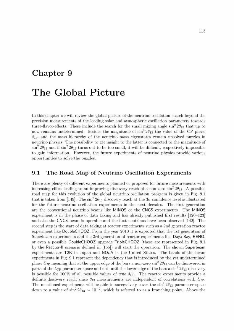
113

Chapter 9

The Global Picture

In this chapter we will review the global picture of the neutrino oscillation search beyond theprecision measurements of the leading solar and atmospheric oscillation parameters towardsthree-flavor-effects. These include the search for the small mixing angle sin2 2θ13 that up tonow remains undetermined. Besides the magnitude of sin2 2θ13 the value of the CP phaseδCP and the mass hierarchy of the neutrino mass eigenstates remain unsolved puzzles inneutrino physics. The possibility to get insight to the latter is connected to the magnitude ofsin2 2θ13 and if sin2 2θ13 turns out to be too small, it will be difficult, respectively impossibleto gain information. However, the future experiments of neutrino physics provide variousopportunities to solve the puzzles.

9.1 The Road Map of Neutrino Oscillation Experiments

There are plenty of different experiments planned or proposed for future measurements withincreasing effort leading to an improving discovery reach of a non-zero sin2 2θ13. A possibleroad map for this evolution of the global neutrino oscillation program is given in Fig. 9.1that is taken from [149]. The sin2 2θ13 discovery reach at the 3σ confidence level is illustratedfor the future neutrino oscillation experiments in the next decades. The first generationare the conventional neutrino beams like MINOS or the CNGS experiments. The MINOSexperiment is in the phase of data taking and has already published first results [120–123]and also the CNGS beam is operable and the first neutrinos have been observed [142]. Thesecond step is the start of data taking at reactor experiments such as a 2nd generation reactorexperiment like DoubleCHOOZ. From the year 2010 it is expected that the 1st generation ofSuperbeam experiments and the 3rd generation of reactor experiments like Daya Bay, RENO,or even a possible DoubleCHOOZ upgrade TripleCHOOZ (these are represented in Fig. 9.1by the Reactor-II scenario defined in [155]) will start the operation. The shown Superbeamexperiments are T2K in Japan and NOνA in the United States. The bands of the beamexperiments in Fig. 9.1 represent the dependency that is introduced by the yet undeterminedphase δCP meaning that at the upper edge of the bars a non-zero sin2 2θ13 can be discovered inparts of the δCP parameter space and not until the lower edge of the bars a sin2 2θ13 discoveryis possible for 100% of all possible values of true δCP. The reactor experiments provide adefinite discovery reach since θ13 measurements are independent of correlations with δCP.The mentioned experiments will be able to successively cover the sin2 2θ13 parameter spacedown to a value of sin2 2θ13 ∼ 10−2, which is referred to as a branching point. Above the

114 CHAPTER 9. The Global Picture

2005 2010 2015 2020 2025 2030Year

10-5

10-4

10-3

10-2

10-1

100

sin2

2Θ13

disc

over

yre

achH3

ΣL

CHOOZ+Solar excluded

Branching pointConv. beams

Superbeams+Reactor exps

Superbeam upgrades

Ν-factories

MINOSCNGSD-CHOOZT2KNOîAReactor-IINOîA+FPD2ndGenPDExpNuFact

Figure 9.1: The possible global evolution of the sin2 2θ13 discovery reach at the 3σ confidence level as afunction of time. The bands indicate the region where a non-zero true value of sin2 2θ13 could be established atthe 3σ confidence level, i.e. sin2 2θ13 = 0 can be excluded, depending on the actual true value of the phase δCP.Below the lower edge of the bands a non-zero true value of sin2 2θ13 could be established independent for 100%of the δCP parameter space. The assumed true values for the other oscillation parameters are sin2 2θ12 = 0.83,∆m2

21 = 8.2 · 10−5 eV2, sin2 2θ23 = 1, and ∆m231 = +2.5 · 10−3 eV2 (normal hierarchy assumed) very close

to the true parameters assumed throughout the previous chapters of this work. Systematics, correlations anddegeneracies are taken into account. This figure is taken from [149].

branching point the measurements are mainly affected by systematical uncertainties and thematter density uncertainty, while for values below the branching point reactor experimentsget highly limited by the systematical uncertainties and the intrinsic beam background atSuperbeam experiments starts to limit the potential. So, to reach for values of sin2 2θ13

below the branching point, upgrades of the Superbeam experiments with higher statistics oreven better β-Beams or a Neutrino Factory are required. Additionally, the branching pointapproximately indicates the theoretical branching point, that separates the large sin2 2θ13

regime, where sin2 2θ13 still can be accidentally small compared to the other mixing angles, andthe small sin2 2θ13 regime, where the smallness of sin2 2θ13 implies an underlying symmetrythat suppresses sin2 2θ13. As can be read off from Fig. 9.1, this branching point should bereached within the next ten years. Beyond the year 2015 more dedicated experiments arerequired and the first step can be provided by an upgrade of the Superbeam experiments.Note, that Fig. 9.1 is taken from [149], a report for the Proton Driver at the FermiLab, so onlyUS strategies are shown here. Note, that also the upgrade T2HK of the T2K Superbeam inJapan and the SPL Superbeam at CERN are planned to operate at the comparable magnitudeof intermediate sin2 2θ13. These upgraded Superbeam experiments provide discovery potential

9.2 Promising Future Experiments 115

below the branching point and even cover the parameter space partially down to sin2 2θ13 ∼10−3. Further candidates for this regime are low γ β-Beams. However, for even smallersin2 2θ13 < 10−3 flavor pure neutrino beam experiments as a medium to high γ β-Beam ora Neutrino Factory are required Here, only a standard Neutrino Factory is shown but we havedemonstrated that also β-Beam are able to cover this regime in Chapter 7 and we will addressthis point in the next Sections. The intended time schedule as indicated in Fig. 9.1 for thiskind of experiments is beyond 2025. The rapid increase of the Neutrino Factory discovery reachat mid time of data taking is due to the switching of beam polarities, i.e. between neutrinoand anti-neutrino running which provides degeneracy resolving potential and thus improvesthe discovery reach immediately by one order of magnitude.

9.2 Promising Future Experiments

It should be kept in mind that the time-line evolution discussed in the last subsection assumesthat no signal has been observed in between. Of course, the reactor experiments or 1st gen-eration of Superbeams are possible to discover a large non-zero sin2 2θ13 during their runtime.This certainly would change the picture and one should aim for a precise measurement ofsin2 2θ13 and also δCP. This is the reason why we will now discuss the performance of possiblepromising next generation future experiments in the regime of large sin2 2θ13 ∼ 10−1. Afterthat we will discuss different options for intermediate sin2 2θ13 where the resolving of thedegeneracies has to be focused and finally we will address the reach in small sin2 2θ13.

Large sin2 2θ13

We will now focus on the scenario of large sin2 2θ13 = 10−1. Such a large value will be dis-covered at the 1st and 2nd generation of future reactor experiments and at the 1st generationof Superbeam experiments. The reactor experiments will provide a clean measurement ofsin2 2θ13 without parameter correlations with δCP. The measurement at the 1st generationof Superbeam experiments will be correlated with the phase δCP but it is very unlikely thatone can gain information on δCP due to the (sin2 2θ13, δCP)-degeneracy. Still, the whole pa-rameter space of δCP will be contained in the allowed region. However, the combination ofthe complementary data sets of reactor experiments and Superbeams start to disfavor someregions of the δCP parameter space to some extend. Still this effect will be also spoiled bythe sign-degeneracy and it will not be possible to distinguish CP violation from CP conser-vation [140, 141]. So, also in this large sin2 2θ13 scenario more dedicated experiments likeupgraded Superbeam experiments, β-Beams, or a Neutrino Factory will be required to shedlight to the puzzle of δCP and the mass hierarchy of the neutrinos.

The performance of the defined β-Beam and Neutrino Factory scenarios and a representativeof the upgraded Superbeam experiments T2HK∗ in terms of discovery potential of sin2 2θ13

(dark/blue bars), CP violation (red/medium grey bars), and the mass hierarchy (green/brightgrey bars) is summarized in Fig. 9.2 for true sin2 2θ13 = 10−1. The bars indicate the fraction of(true) δCP where the respective parameter can be discovered at the 3σ confidence level. Fromtop to bottom the detector effort is quantitatively increased from single detector scenarios totriple detector scenarios. As expected all experiment scenarios can discover the large sin2 2θ13

independent of δCP. Also, since sin2 2θ13 is large, most of the scenarios can determine themass hierarchy in 100% of the δCP parameter space. Only the shorter baseline experimentsare not able to observe matter effects and distinguish normal from inverted hierarchy in large

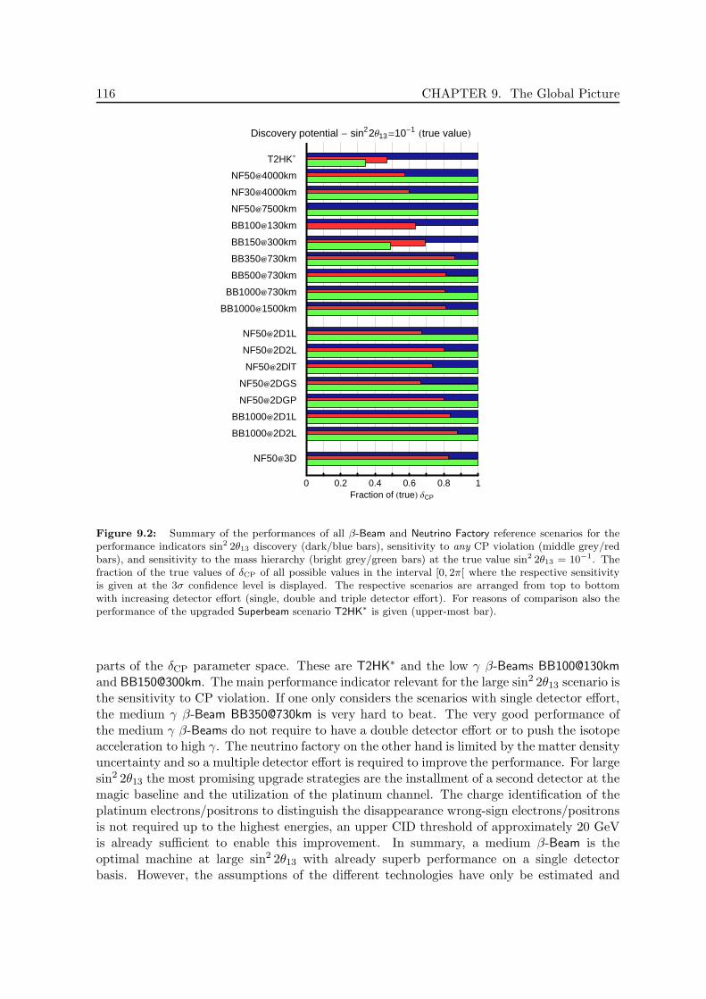
116 CHAPTER 9. The Global Picture

Discovery potential - sin22Θ13=10-1Htrue valueL

T2HK*

NF504000km

NF304000km

NF507500km

BB100130km

BB150300km

BB350730km

BB500730km

BB1000730km

BB10001500km

NF502D1L

NF502D2L

NF502DlT

NF502DGS

NF502DGP

BB10002D1L

BB10002D2L

NF503D

0 0.2 0.4 0.6 0.8 1Fraction of HtrueL ∆CP

Figure 9.2: Summary of the performances of all β-Beam and Neutrino Factory reference scenarios for theperformance indicators sin2 2θ13 discovery (dark/blue bars), sensitivity to any CP violation (middle grey/redbars), and sensitivity to the mass hierarchy (bright grey/green bars) at the true value sin2 2θ13 = 10−1. Thefraction of the true values of δCP of all possible values in the interval [0, 2π[ where the respective sensitivityis given at the 3σ confidence level is displayed. The respective scenarios are arranged from top to bottomwith increasing detector effort (single, double and triple detector effort). For reasons of comparison also theperformance of the upgraded Superbeam scenario T2HK∗ is given (upper-most bar).

parts of the δCP parameter space. These are T2HK∗ and the low γ β-Beams BB100@130kmand BB150@300km. The main performance indicator relevant for the large sin2 2θ13 scenario isthe sensitivity to CP violation. If one only considers the scenarios with single detector effort,the medium γ β-Beam BB350@730km is very hard to beat. The very good performance ofthe medium γ β-Beams do not require to have a double detector effort or to push the isotopeacceleration to high γ. The neutrino factory on the other hand is limited by the matter densityuncertainty and so a multiple detector effort is required to improve the performance. For largesin2 2θ13 the most promising upgrade strategies are the installment of a second detector at themagic baseline and the utilization of the platinum channel. The charge identification of theplatinum electrons/positrons to distinguish the disappearance wrong-sign electrons/positronsis not required up to the highest energies, an upper CID threshold of approximately 20 GeVis already sufficient to enable this improvement. In summary, a medium β-Beam is theoptimal machine at large sin2 2θ13 with already superb performance on a single detectorbasis. However, the assumptions of the different technologies have only be estimated and

9.2 Promising Future Experiments 117

considerable R&D is required before the final technology discussion can be made. Beforea dedicated experiment like a Neutrino Factory or a medium γ β-Beam is to be installedthe Superbeam experiments with possible upgrades are very likely to already constrain theδCP parameter space quite efficiently. Also low γ β-Beam scenarios such as the CERN-Frejusγ = 100 baseline scenario (similar to BB100@130km) are very promising candidates. TheL=130 km baseline was also proposed to combine two experiment technologies, the SPLSuperbeam and the γ = 100 β-Beam with the same megaton Water Cherenkov detector [247].Then the CP and the T conjugate channels could be measured at one site and furthermoresystematical uncertainties can be reduced since the β-Beam signal event type correspondsto the background at the Superbeam and vice versa. The potential of such a scenario wasinvestigated in [187]. It was realized that the combination of T and CP conjugated channelsat such a facility improve quite significantly the sensitivity to the mass hierarchy even at thevery small baselines [248]. Another possibility with even more promising potential is impliedby the combination of the T2HK Superbeam with a low γ β-Beam similar to BB150@300km.

Intermediate sin2 2θ13

If sin2 2θ13 is not discovered at the reactor experiments and first generation of Superbeam ex-periments the large sin2 2θ13 regime will be excluded and a new lower limit can be establishedwith sin2 2θ13 . 10−2. Following the time schedule of Fig. 9.1 this could be the case approxi-mately in the year 2015 (depending on the actual individual startup of the single experiments).Beyond this point more sophisticated experiments are required to take over. Superbeam up-grades, low γ β-Beam experiments or even combinations of these are thinkable to be candidatesto start exploiting the next smaller regime of intermediate 10−3 < sin2 2θ13 < 10−2, howevernot the complete parameter space can be covered and especially the determination of the masshierarchy is difficult. Although the δCP parameter space can be well covered by a medium γβ-Beam sufficient potential to measure the sign of ∆m2

31 is also difficult for such a scenariodue to the still relative small baseline. Therefore, a Neutrino Factory experiment is mostpromising to provide excellent discovery potential for all three puzzles, sin2 2θ13, δCP, and themass hierarchy, but the problems due to parameter correlations and the eight-fold degeneracyhave to be addressed. This means that multiple detector scenarios have to be considered.

The performance of the defined β-Beam and Neutrino Factory scenarios and a representativeof the upgraded Superbeam experiments T2HK∗ in terms of discovery potential of sin2 2θ13

(dark/blue bars), CP violation (red/medium grey bars), and the mass hierarchy (green/brightgrey bars) is summarized in Fig. 9.3 for true sin2 2θ13 = 10−3. The bars indicate the fraction of(true) δCP where the respective parameter can be discovered at the 3σ confidence level. Fromtop to bottom the detector effort is quantitatively increased from single detector scenarios totriple detector scenarios. The discovery of θ13 is only a problem for the Superbeam and thelow γ β-Beam scenarios. Already medium γ β-Beams with a Water Cherenkov detector, highγ β-Beams and a Neutrino Factory can discover a non-zero sin2 2θ13 = 10−3 independent ofthe true δCP. However, already for intermediate sin2 2θ13 the performance of the β-Beamsgets disadvantageous compared to the Neutrino Factory scenarios because the mass hierarchydetermination potential is limited. This can only be restored by a high γ β-Beam with adouble detector effort and a second baseline L∼3000 km as BB1000@2D2L. The δCP discoverypotential of the β-Beams and the Neutrino Factory scenarios is very similar with slight leadfor the medium and high γ β-Beams. The degeneracy resolving at the Neutrino Factory canbe facilitated by double detector effort and at intermediate sin2 2θ13 a second detector at

118 CHAPTER 9. The Global Picture

Discovery potential - sin22Θ13=10-3Htrue valueL

T2HK*

NF504000km

NF304000km

NF507500km

BB100130km

BB150300km

BB350730km

BB500730km

BB1000730km

BB10001500km

NF502D1L

NF502D2L

NF502DlT

NF502DGS

NF502DGP

BB10002D1L

BB10002D2L

NF503D

0 0.2 0.4 0.6 0.8 1Fraction of HtrueL ∆CP

Figure 9.3: Summary of the performances of all β-Beam and Neutrino Factory reference scenarios for theperformance indicators sin2 2θ13 discovery (dark/blue bars), sensitivity to any CP violation (middle grey/redbars), and sensitivity to the mass hierarchy (bright grey/green bars) at the true value sin2 2θ13 = 10−3. Thefraction of the true values of δCP of all possible values in the interval [0, 2π[ where the respective sensitivityis given at the 3σ confidence level is displayed. The respective scenarios are arranged from top to bottomwith increasing detector effort (single, double and triple detector effort). For reasons of comparison also theperformance of the upgraded Superbeam scenario T2HK∗ is given (upper-most bar).

the magic baseline or a lower energy threshold at a Hybrid detector are the most promisingscenarios. The inclusion of the additional channels, silver or platinum, only helps to someextend to resolve the degeneracies and if the assumptions of the optimistic scenarios cannot beachieved, the improvement cannot justify the detector effort that is involved with the inclusion.The combination of magic baseline and a Hybrid detector at L=4000 km is the ultimateoptimized scenario at intermediate sin2 2θ13 and provides excellent discovery potential.

Small sin2 2θ13

From an experimental point of view, the worst case scenario is a very small sin2 2θ13 sinceadditionally to the parameter correlations and degeneracies, the decreasing statistics in theappearance channel become a limiting factor. So, the reach of the experiment scenarios getsimportant, i.e. to which small values of sin2 2θ13 < 10−3 a reasonable discovery potential canbe maintained.

The performance of the defined β-Beam and Neutrino Factory scenarios and a representative

9.2 Promising Future Experiments 119

Discovery potential - 50% fraction of HtrueL ∆CP

T2HK*

NF504000km

NF304000km

NF507500km

BB100130km

BB150300km

BB350730km

BB500730km

BB1000730km

BB10001500km

NF502D1L

NF502D2L

NF502DlT

NF502DGS

NF502DGP

BB10002D1L

BB10002D2L

NF503D

10-5 10-4 10-3 10-2 10-1

True value of sin22Θ13

Figure 9.4: Summary of the performances of all β-Beam and Neutrino Factory reference scenarios forthe sin2 2θ13 reach of the performance indicators sin2 2θ13 discovery (dark/blue bars), sensitivity to any CPviolation (middle grey/red bars), and sensitivity to the mass hierarchy (bright grey/green bars). The barsindicate for which true values of sin2 2θ13 the respective sensitivities are given for at least 50% of all possibletrue values of δCP in the interval [0, 2π[at the 3σ confidence level. The respective scenarios are arrangedfrom top to bottom with increasing detector effort (single, double and triple detector effort). For reasons ofcomparison also the performance of the upgraded Superbeam scenario T2HK∗ is given (upper-most bar).

of the upgraded Superbeam experiments T2HK∗ in terms of discovery potential of sin2 2θ13

(dark/blue bars), CP violation (red/medium grey bars), and the mass hierarchy (green/brightgrey bars) is summarized in Fig. 9.4 considering the discovery reach to small sin2 2θ13. Thebars indicate the sin2 2θ13 parameter space, where the respective parameters can be discoveredfor at least 50% of the δCP parameter space at the 3σ confidence level. Here, the main interestlies on those scenarios from Fig. 9.4 with a discovery potential that reaches to values of smallsin2 2θ13 < 10−3. The most promising scenario is a Neutrino Factory since only the NeutrinoFactory scenarios provide a θ13 discovery potential for values sin2 2θ13 < 10−4 already for thesingle detector effort setups. Additionally, at a Neutrino Factory the discovery potential todetermine the neutrino mass hierarchy can be maintained to smallest sin2 2θ13 ∼ 10−4. Thebest optimizing strategy to increase the discovery reach of a standard NF50@4000km turnsout to be the Hybrid detector scenario with the lower threshold or even a combination withthe magic baseline with a triple detector effort. The only optimizing strategy for β-Beams toremain competitive for small sin2 2θ13 in terms of all three performance indicators requires a

120 CHAPTER 9. The Global Picture

high γ scenario with two Totally Active Scintillator detectors at two different baselines. Oneof these baselines at L∼3000 km to improve the discovery reach for the determination of themass hierarchy to sin2 2θ13 ∼ 10−4. However, we summarize that the optimal technology forsmall sin2 2θ13 turns out to be a Neutrino Factory with a second detector at the magic baselineand possibly improved detector performance, i.e. a lower energy threshold.

121

Chapter 10

Summary and Conclusions

In this work, we have discussed the performance of the sophisticated neutrino oscillationlong baseline scenarios of β-Beam experiments and Neutrino Factory experiments. The mainfocus was set on the investigation of the features of the possible optimization strategies andtechnical considerations of the respective experiment characteristics in the search for three-flavor effects in the observable appearance channels at the respective experiments and theimplied sensitivities to the small mixing angle sin2 2θ13, the Dirac phase δCP, and the masshierarchy of the neutrino mass eigenstates.

The optimization of the experiment scenarios was discussed in terms of the baseline Land the neutrino energy Eν for single detector scenarios. In the simulations of the β-Beamexperiments, two different detector technologies were considered, a Water Cherenkov detectorand a Totally Active Scintillator detector. The Water Cherenkov detector is suitable for lowand medium γ β-Beams, but for high γ scenarios a different detector technology is requiredbecause the Water Cherenkov detector is limited by the background from single pion pro-duction in neutral-current reactions and the pions can be misidentified as muons. Hence, forthe high γ scenarios only the Totally Active Scintillator detector technology was considered,that provides excellent background rejection even at higher energies and additionally betterenergy resolution. The Totally Active Scintillator detector was also considered for mediumγ scenarios to allow for a comparison of the detector technologies at intermediate neutrinoenergies. Similarly, the discussion of the optimization of a Neutrino Factory experiment in-volved the choice of the baseline L and the neutrino energy, controlled by the energy of thestored parent muons Eµ. This optimization was first performed for a single detector scenariofocusing on the measurement of the so-called golden channel νe → νµ that can be measuredat a Magnetized Iron detector which allows for a separation of the so-called wrong sign muonscoming from the dominating disappearance channel.

For both, the β-Beam and the Neutrino Factory scenarios, we found that the optimizationin terms of sensitivity to sin2 2θ13 and sensitivity to CP violation is very similar since foroptimal performance in both sensitivities, the (sin2 2θ13, δCP)-degeneracy has to be resolved.Consequently, there has to be no trade-off for the optimization. However, if also a good abilityto resolve the sign-degeneracy and determine the existing mass hierarchy of the neutrino masseigenstates is requested, the situation becomes more complicated because optimal performancefor sensitivity to CP violation and sensitivity to the mass hierarchy cannot be optimizedsimultaneously and multi-detector scenarios are required for an overall optimized performance.For the neutrino factory, this implies one detector at L ∼ 4000 km for optimal CP sensitivity

122 CHAPTER 10. Summary and Conclusions

and one detector at the magic baseline L ∼ 7500 km for excellent sign-degeneracy resolvingpotential. The β-Beam on the other hand is mainly a very powerful tool for measurementsof sin2 2θ13 and δCP and is less sensitive to the mass hierarchy because the baselines aresmaller than Neutrino Factory baselines and matter effects do not play such an importantrole. However, the discussed high γ scenarios at relatively large baselines provided reasonablesensitivities to the mass hierarchy and also two-detector scenarios turned out to increase thepotential enormously.

Beyond the elementary optimization strategies in terms of experiment baselines and neu-trino energies, also different technical considerations of the β-Beam and Neutrino Factory sce-narios were discussed. For both kinds of experiments we have shown that the actual ratio theneutrino and anti-neutrino runtime fractions does not play a very significant role and splittingthe runtime in two equal phases of neutrino and anti-neutrino running is well justified.

Since the β-Beam experiments do not provide the possibility to measure the leading at-mospheric parameters in the dominating disappearance channel, as is the case at a NeutrinoFactory, it was expected that parameter correlations with the atmospheric parameters wouldheavily affect the sensitivities to sin2 2θ13, δCP, and the mass hierarchy at a the β-Beam sce-narios. We have presented the impact of the inclusion of external disappearance data from thefirst generation Superbeam experiment T2K and it could be seen that the external informa-tion on the leading atmospheric parameters indeed gives a large impact in the performance.Hence, the disadvantage of a β-Beam compared to a Neutrino Factory is the dependency onexternal informations, whereas the Neutrino Factory is capable of measuring the leading at-mospheric parameters in the disappearance channel. Note, that a β-Beam cannot participatein the search for deviations from maximal mixing sin2 2θ23 due the missing information onthe leading atmospheric parameters.

Furthermore, we discussed the impact of a possible γ-scaling of the number of isotopedecays at a β-Beam if higher γ accelerations are considered, since the usually discussed numberof decays is treated constant for low, medium, and high γ scenarios. This of course requestsan appropriate scaling of the storage ring and the sufficient injection of accelerated isotopes.It was observed that a possible γ-scaling can indeed destroy the excellent sensitivities that canbe achieved at medium and high γ β-Beams and going to higher γ scenarios is only reasonableif the γ scaling of the number of isotope decays can be kept at a minimum.

For the optimization of the Neutrino Factory scenarios we have additionally discussed thepossibility of an inclusion of secondary channels, the silver channel νe → ντ and the plat-inum channel νµ → νe, to help resolving the degeneracies at intermediate sin2 2θ13 since theperformance of the golden channel is to some extend limited due to the (sin2 2θ13, δCP)- andsign-degeneracies. This effect is mainly observed at Neutrino Factory experiments since a Neu-trino Factory is not operated at the oscillation maximum due to the CID cut that is requiredto identify the wrong-sign muons coming from the dominating disappearance channel. Atβ-Beam experiments the effects of the degeneracies are not as large as for Neutrino Factoryexperiments since the β-Beam beam neutrino spectrum perfectly covers the first oscillationmaximum. It was shown that the standard assumptions about the included silver and plat-inum channels at a Neutrino Factory are not sufficient to significantly improve the resolving ofthe degeneracies and more optimistic assumptions have to be realized that are hardly feasible.For the silver channel a dedicated increase in the detector mass of the silver channel detector,an Emulsion Cloud Chamber detector, is required and also the detection of the τ decay inall decay channels and not only the leptonic decays as was assumed for the standard silverchannel. The optimistic assumptions for the platinum channel involved the detector mass of

CHAPTER 10. Summary and Conclusions 123

50 kt and the extremely optimistic assumption of a possible electron/positron discriminationup to the highest energies. Hence, we have to conclude that the usefulness of the additionalchannels for helping to resolve the degeneracies at intermediate sin2 2θ13 is questionable.

We have nevertheless observed that the platinum channel is very promising in the regimeof large sin2 2θ13 where the main limiting factor at a Neutrino Factory is the matter densityuncertainty along the baseline. This is due to the fact that the platinum channel is the Treversed channel of the golden channel, whereas switching from neutrino to anti-neutrinorunning compares the CP conjugated golden channels. In vacuum oscillations the T reversedand CP conjugated channels carry the same information and only statistics could be increased,however in oscillations in matter the platinum channel does not involve the reversed mattereffect as the CP conjugated golden channel and the inclusion of the platinum channel givesthe possibility to distinguish the intrinsic and extrinsic contributions to CP violation. So,the sensitivity to CP violation is significantly improved. We found that this effect does notrequire the very optimistic assumptions for the platinum channel detection and in this caseit is sufficient to achieve an upper electron/positron CID threshold of about 15-20 GeV.However, this is still a demanding requirement since electrons tend to shower early in thedetector and the observation of the track curvature is difficult. The CID is required toreduce the background in the platinum channel coming from the electrons/positrons from thedisappearance channel νe → νe comparable to the requirement of the muon CID in the goldenchannel.

A very interesting observation for the Neutrino Factory scenarios was given when we dis-cussed the performance potential of a Neutrino Factory scenario at L ∼ 4000 km with alower stored parent muons energy Eµ = 30 GeV compared to the standard assumption ofEµ = 50 GeV. We found that the lower neutrino energy Neutrino Factory scenario providesthe very similar performance for all three performance indicators and it may not be necessaryto accelerate the muons to the highest energies. This gives the interesting opportunity toeconomize the effort in the construction of the acceleration complex.

Furthermore, we have discussed an optimized golden channel detection with a lower energythreshold and better energy resolution. This could be achieved with an Hybrid detector, i.e. acombined detector technology for higher and lower energies. Due to the lower energy thresholdthe oscillation maximum at lower energies would become accessible and the potential to resolvethe degeneracies is significantly improved. Such a scenario gives the best Neutrino Factoryoptimizing potential at intermediate and small sin2 2θ13 and can only be beaten for largesin2 2θ13 by the inclusion of an optimized platinum channel or a double detector scenariowith a golden channel measurement at L ∼ 4000 km combined with the golden channelmeasurement at the magic baseline.

We have analyzed the potential of a low γ β-Beam scenario comparable to the γ = 100CERN-Frejus baseline scenario and it was shown that a low γ β-Beam cannot compete withhigher γ β-Beams or Neutrino Factory experiments mainly due to the lack of sensitivity to themass hierarchy even in the regime of large sin2 2θ13. However, it became apparent that lowγ β-Beams can compete and even slightly outperform the second generation of Superbeamscenarios, in our discussions represented by the T2HK experiment. We proposed a low γ β-Beam at the baseline of L ∼ 300 km and γ = 150 which is accessible at an accelerator complexof the size of the SPS that provides a considerably better performance as the γ = 100 β-Beamat the similar technical effort. Note, that the baseline of L ∼ 300 km matches the baseline ofthe baseline between the J-PARC accelerator complex in Japan and the designated location ofthe Hyper-Kamiokande megaton Water Cherenkov detector. Just as the CERN-Frejus baseline,

124 CHAPTER 10. Summary and Conclusions

this baseline would also allow for a combination of a Superbeam and a β-Beam at the samebaseline to improve the sensitivity to the mass hierarchy.

The discussion of the medium β-Beam scenarios indicated that in principle it is not re-quired to aim for high γ scenarios since the sensitivity to CP violation is already excellentat medium γ β-Beams and the sensitivity to the mass hierarchy is only slightly improved.High γ scenarios are only interesting if two-detector scenarios are considered to impressivelyimprove the sin2 2θ13 reach in the sensitivity to the mass hierarchy.

To summarize, in the regime of large 10−2 . sin2 2θ13 . 10−1 the medium γ β-Beamscenarios give the best performance since mainly the sensitivity to CP violation discriminatesthe best experiment technology because θ13 and mass hierarchy discovery potential is excellentat Neutrino Factory experiments and higher γ β-Beam experiments. However, the combinationof the data of upgraded Superbeam experiments, reactor experiments and possibly also low γβ-Beams already will give very good performances and higher γ β-Beams or Neutrino Factoryscenarios are not necessarily required.

In the regime of intermediate 10−3 . sin2 2θ13 . 10−2 the most promising candidates aremedium γ β-Beams for measurements of sin2 2θ13 and δCP. Unfortunately, medium γ β-Beamsloose the sensitivity to the mass hierarchy in this regime of sin2 2θ13 and high γ β-Beams andNeutrino Factory experiments at large baselines become preferable. However, the NeutrinoFactory requires optimization of the golden channel, i.e. a detector at the magic baseline inorder to successfully resolve the parameter degeneracies at intermediate sin2 2θ13. The aimfor a lower threshold due to a Hybrid detector scenario is extremely promising to give furtheroptimization of the Neutrino Factory performance.

Finally, if the regime of small sin2 2θ13 . 10−3 is considered, clearly the Neutrino Fac-tory scenario is the ultimate machine because the discovery potential reaches to very smallsin2 2θ13 . 10−4 for all three performance indicators sensitivity to sin2 2θ13, CP violation,and the sensitivity to the mass hierarchy. The best performance can be achieved if a lowerthreshold at a Hybrid detector scenario can be achieved and the sensitivity reach to themass hierarchy is impressively improved with additional measurements at the magic baseline.The combination of the Hybrid detector at L ∼ 4000 km and the magic baseline measure-ments give the ultimate optimized Neutrino Factory in the regime of small sin2 2θ13. β-Beamscenarios cannot compete with Neutrino Factory experiments in the regime of small sin2 2θ13,because even an ultimate two-detector high γ β-Beam cannot establish as good mass hierarchysensitivities as a Neutrino Factory.

125

Appendix A

The General Long Baseline

Experiment Simulator

The General Long Baseline Experiment Simulator GLoBES [220, 221, 249] is a softwarepackage that allows to simulate future neutrino oscillation long baseline experiments andanalyze their potential to measure neutrino oscillation parameters. Within GLoBES theexperiments are described in an Abstract Experiment Definition Language, so-called AEDL,that allows to simulate a variety of different detector technologies combined with point-likeneutrino sources. Thus, besides beam-based experiments as conventional beam experiments,Superbeams, β-Beams or Neutrino Factory experiments also neutrino reactor experimentscan be simulated. Additionally, very different kinds of systematical uncertainties, as e.g.normalization and energy calibration errors can be included to the simulation and the matterprofile along the baseline can be treated accurately including uncertainties. GLoBES providesthe calculation of the exact three-flavor oscillation probabilities, in vacuum and in matter andthe calculation of event rates as well as simple Poisson χ2 calculation. More sophisticatedGLoBES functions allow to treat the full multi-parameter correlations and degeneracies bythe ∆χ2-projection of the six-dimensional parameter space to planes or axes in the parameterspace.

The GLoBES software is available from the web and can be found at

http://www.mpi-hd.mpg.de/lin/globes/

in the newest version GLoBES 3.0. Together with the software, pre-defined experiment de-scribing AEDL files are distributed, and some have been used in modified versions in thesimulations throughout this work. The β-Beam simulations can be reproduced with the filesBBvar_WC.glb that describes a variable β-Beam with a Water Cherenkov detector and BB-

var_TASD.glb that describes a variable β-Beam with a Totally Active scintillator detector.The β-Beam fluxes are provided as built-in functions and only the γ,the endpoint energiesof the considered isotopes, and the number of isotope decays per year have to be set. TheNeutrino Factory simulations can be partially reproduced with the files NFvar.glb that de-scribes a variable golden channel Neutrino Factory with a 50 kt Magnetized Iron detector,NF_GoldSilver.glb that describes the same golden channel as above in combination withthe standard silver channel scenario, and the file NF_hR_lT.glb that describes an optimizedgolden channel with better energy resolution and lower energy threshold (in this work labeled

126 CHAPTER A. The General Long Baseline Experiment Simulator

as hybrid detector scenario). The description for the platinum channel and the optimisticsilver channel are not distributed with GLoBES. The Neutrino Factory fluxes are provided asbuilt-in functions and only the parent energy of the stored muons and the number of storedmuons have to be set. Furthermore, the results for the Superbeam T2HK can be reproducedwith the file T2HK.glb.

For performing simulations, the flux is mapped into an energy-binned event rate vectorfor different channels, signals and backgrounds. This mapping takes into account the oscilla-tion probabilities (matter effects included accordingly to the respective baseline and neutrinoenergy), neutrino cross sections for the selected channels, and the AEDL described detectorresponse that includes the fiducial detector mass, signal efficiencies, background rejection fac-tors, energy dependent threshold functions, and the energy resolution of the detector. At thebeginning of all simulations the event rate vector for an assumed set of so-called true oscillationparameter values is calculated. If not explicitely stated otherwise, the true parameter valuesfor the leading oscillation parameters sin2 2θ12, ∆m2

21, sin2 2θ23, ∆m231 used in the simulations

throughout this work are the best-fit parameters given in Eq. (5.25). The true parameters ofsin2 2θ13 and δCP depend on the considered performance indicators. This event rate vectoris then treated as the simulated data of the simulated experiments. The GLoBES functionsare then used to fit the simulated data with fit values by using the same mapping functionto calculate simulated expected rate vectors as described above and calculate the respectivePoisson χ2 value. Additionally the defined χ2 function includes the systematical uncertaintieslike normalization errors, energy calibration errors, or the matter density uncertainty. Theparameter space of fit values is effectively scanned by using the marginalization features ofGLoBES by projecting the ∆χ2 to the respective axes of the parameter space by includingall possible degenerate solutions in the six-dimensional parameter space. Throughout thiswork only projections to the sin2 2θ13 and δCP axis are required for the simulations while thesensitivities to mass hierarchy are calculated by marginalizing over all parameters to find thelocal minimum of the sign-degenerate solution in the six-dimensional parameters space.

Further details of simulations with the GLoBES software together with the detailed de-scription of the event rate calculation, the implementation of systematical uncertainties, andthe χ2 calculation within GLoBES can be found in the GLoBES manual [223].

127

Appendix B

Performance Indicators

Throughout this work, we have made use of the so-called performance indicators to describethe physics potential of neutrino oscillation long baseline experiments, such as a β-Beam ora Neutrino Factory. The performance indicators were used to optimize different experimentscenarios in terms of baseline and neutrino energy, to describe the impact of different effectsto the overall performance or to compare the performance of the different experiment anddetector technologies. The performance indicators shall describe the potential of the consid-ered experiments to make discoveries of three-flavor effects, i.e. measure a non-zero sin2 2θ13

or establish CP violation or the mass hierarchy of the neutrinos. In the following, all differentdiscussed performance indicators are listed and a detailed definition is given.

Sensitivity limit to sin2 2θ13

The sensitivity limit to sin2 2θ13 is the largest fit value sin2 2θfit13 that still fits an assumed

true value sin2 2θtrue13 = 0 at the chosen confidence level after marginalization over all other

oscillation parameters δCP, sin2 2θ12, ∆m221, sin2 2θ23, and ∆m2

31 where both degenerate fitsolutions are considered: ∆m2

31 > 0 and ∆m231 < 0. Systematics are taken into account

and the marginalization process also includes the matter density ρ to account for the matterdensity uncertainty ∆ρ (constrained by a pull term). For the set of assumed true parametersa normal mass hierarchy with (∆m2

31)true > 0 is chosen only, since the assumption of inverted

hierarchy gives essentially the same sin2 2θ13 sensitivity limit. This was demonstrated in theappendix of [140] where further details of the computation of the sin2 2θ13 sensitivity limithave been visualized. The sensitivity limit to sin2 2θ13 can be interpreted as the achievablelower bound on sin2 2θ13 at the considered experiment in case of a non-observation.

Discovery reach for sin2 2θ13

The discovery reach for sin2 2θ13 is the smallest true value sin2 2θtrue13 for that the fit value

sin2 2θfit13 = 0 could still be excluded at the chosen confidence level, i.e. a non-zero sin2 2θ13

could still be discovered. The discovery reach for sin2 2θ13 depends strongly on the true valueof the phase δCP. As for the sensitivity limit, a marginalization over all other oscillationparameters δCP, sin2 2θ12, ∆m2

21, sin2 2θ23, and ∆m231 is performed. Systematics are taken

into account and the marginalization process also includes the matter density ρ to accountfor the matter density uncertainty ∆ρ (constrained by a pull term).

128 CHAPTER B. Performance Indicators

Sensitivity to maximal CP violation

Sensitivity to maximal CP violation is given at the chosen confidence level for a true valueof sin2 2θtrue

13 in case of maximal CP violation (either δtrueCP = π/2 or δtrue

CP = 3π/2), if theCP conserving fit values δfit

CP = 0 and δfitCP = π can be excluded at this confidence level

after marginalization over all other oscillation parameters sin2 2θ13, sin2 2θ12, ∆m221, sin2 2θ23,

and ∆m231 where both degenerate fit solutions are considered: ∆m2

31 > 0 and ∆m231 < 0.

Systematics are taken into account and the marginalization process also includes the matterdensity ρ to account for the matter density uncertainty ∆ρ (constrained by a pull term).

Sensitivity to any CP violation

Sensitivity to any CP violation is given at the chosen confidence level for a pair of true valuessin2 2θtrue

13 and δtrueCP , if the CP conserving fit values δfit

CP = 0 and δfitCP = π can be excluded

at this confidence level after marginalization over all other oscillation parameters sin2 2θ13,sin2 2θ12, ∆m2

21, sin2 2θ23, and ∆m231 where both degenerate fit solutions are considered:

∆m231 > 0 and ∆m2

31 < 0. Systematics are taken into account and the marginalizationprocess also includes the matter density ρ to account for the matter density uncertainty∆ρ (constrained by a pull term). Note that a sensitivity to any CP violation can never beestablished for fit values of δCP close to the CP conserving values because of systematical andstatistical uncertainties, i.e. sensitivity to any CP violation is not achievable for a fraction of100% of all possible true values δtrue

CP in the intervals ]0, π[ and ]π, 2π[.

Sensitivity to mass hierarchy

Sensitivity to mass hierarchy is given at the chosen confidence level for a pair of true valuessin2 2θtrue

13 and δtrueCP and the assumption of (∆m2

31)true > 0 (normal hierarchy), if the degener-

ate solution with (∆m231)

fit < 0 (inverted hierarchy) can be excluded at this confidence levelafter marginalization over all oscillation parameters sin2 2θ13, δCP, sin2 2θ12, ∆m2

21, sin2 2θ23,and ∆m2

31. Systematics are taken into account and the marginalization process also includesthe matter density ρ to account for the matter density uncertainty ∆ρ (constrained by a pullterm).

Acknowledgments

First of all I want to express my sincere thanks to my supervisor Prof. Dr. Manfred Lindnerwho introduced me to the very interesting field of neutrino physics and increased my interestin astro-particle physics already during my studies. He gave me the opportunity to travel toconferences and summer schools and experience interesting topics and interesting places allover Europe including Stockholm, Paris, Krakow, and last but not least Heidelberg. I amespecially grateful that he further supported my work after going to Heidelberg and hencemaking it possible that I could finish my thesis in Munich.

I want to thank my long-time collaborators Patrick Huber and Walter Winter who pro-vided me with this nice powerful simulation tool and gave me the opportunity to be a partof the GLoBES team. Especially Patrick required some intense patience since he also sharedthe office with me in the early days and had to listen to all my lazy questions. Why look inthe manual, when the guy who knows it all, sits right besides you? Walter kept motivatingme with the deadlines he commonly brought up in collaborations and showed me in earlystages how to organize team work. Furthermore, he always gave me insight to his simulationtechniques in the days I had to get used to GLoBES.

Also my collaborator Thomas Schwetz deserves my thanks since it was always a pleasureto listen to his thoughts and further comments like “Ja, des is’ muhsam!”.

Of course it was also a great pleasure to collaborate with young guys who I could sharesome knowledge with. So, I really thank Joachim“F.”Kopp and Alex Merle for the discussionswe shared before they left for Heidelberg.

Finally, I want to thank Prof. Dr. Joe Sato from Japan who was a guest in our group andintroduced me to the phenomenologically very nice idea of “high γ” monobeam experimentsand provided me with the demanding task to implement the idea into GLoBES. EspeciallyI am grateful for his patience and very nice personality. “Hats off!” for the one and onlyprofessor who ever joined us in a Kart-Race.

Most of all, I wish to express great thanks to my Mom. She supported me like no one elseover the last, well almost thirty years. Without her motivations I could never have come sofar. Also, I want to thank my Dad who, like my Mom, supported my studies in Munich fromthe beginning and I still benefit from his support because if I look out of the window, thenthere doesn’t seem to be any subway going to Munich anymore.

Lots of incredible thanks to the computer administrators who always kept the computersgoing and provided immediate help if something went wrong: Herbert Muller, Markus MichealMuller, and Stefan Recksiegel.

Furthermore, I want to thank our secretary Karin Ramm for keeping everything going andthe very helpful discussions about the office furniture and the hints regarding the choice of thecolor of the carpet. Yet, I am still very glad that Mato and I did not follow your suggestionsregarding the color of the walls.

Special thanks go out to Prof. Dr. Michael Ratz for providing a nice atmosphere inMunich over the last year and giving me the opportunity to stay in my old office, involvingthe whole “Pimp my Office” thing.

By any means I would like to thank any former members of our group or guests thatcontributed to the very nice atmosphere at T30d: Evgeny Akhmedov, Mathias Anderson,Stefan Antusch, Florian Bauer, Alexander Blum, Marc-Thomas Eisele, Mathias Garny,Srubabati Goswami, Naoyuki Haba, Claudia Hagedorn, Andreas Hohenegger, Patrick Huber,Jorn Kersten, Joachim Kopp, Alexander Merle, Markus Michael Muller, Tommy Ohlsson,Toshihiko Ota, Florian Plentiger, Karin Ramm, Michael Ratz, Werner Rodejohann, JoeSato, Yoshio Sato, Michael Schmidt, Thomas Schwetz, Gerhart Seidl, Alexei Smirnov, andWalter Winter. And of course I also want to thank lots of members of the groups of Prof.Dr. Andrzej Buras and Prof. Dr. Wolfram Weise for contributing to the nice atmosphere.

And now to something completely different. Thanks go out to ...

• .... well, first of all, to all guys and the some girls who joined for having Kart-Races,gambling Poker, going to the cinema, playing Billiard, or going to the “Biergarten”. Itwas a pleasure! You are too many and I am too lazy to give all the names. You knowwho you are.

• .... Jorn, for somehow convincing me to watch movies in the original versions which hada huge impact in the following years.

• .... Tommy, for introducing me to the City of Stockholm and all the nice restaurants.

• .... Werner, for being a cool dude, sharing the passion about Lost with me, and givingaway the hint with “House, M.D.”. See yah in anothah life, brotha!

• .... MMM, for organizing the Kart-Races including the nice web page and all the enjoy-able discussions about comedians and cabaret artists.

• .... the Sneak-Crew Felix, Tobi, and Florian. ... and of course the Ladies.

• .... the whole Crew of the Office 1142 over all those years. Thanks for the patience andplease don’t tell away all the secrets!

• .... Mathias Anderson, for sharing some of the same passions with me: Poker, watchingSnooker, Wong Kar-Wai movies, and the Gilmore Girls.

• .... Damon Lindelof and Carlton Cuse!!!! Furthermore to Tim Kring, Gregory ThomasGarcia and David Shore.

• .... Felix, for listening to my strange theories and being the only guy, one can talk towithout explaining all the mentioned names along the conversation. Come on, there arepeople out there, who refer to Giovanni Ribisi and Jon Favreau as some guys who wereonce guest-starring in “Friends”.

• .... Claudia, for some of the most enjoyable discussions I ever had with a woman andfor reminding me to spend a cake and coffee.

• .... Anton, for nice breaks in our office and the lessons in History and Economics. Bythe way, I was never actually present when you indeed said something critical.

• .... Mato, for well everything, for being the cool office mate, for the discussions aboutPoker, movies, and all the other stuff, for the challenge of confronting me with views Iwould not ever think about, for having stopped tickling me, ...

• .... Elmar, for the“cigarette move”, for the art of unsubstantial conversations, for callingin from time to time, and for the incredible stories you have to tell.

• .... Konstancja, for the very nice days in Krakow and the smilies in the subsequente-mails.

• .... Desideria, for the support of my superstitious mind with the regular placing of theirregular TGiF content.

• .... Felix, Tobi, and Jana for having been there.

133

Bibliography

[1] S. L. Glashow, Partial symmetries of weak interactions, Nucl. Phys. 22 (1961), 579–588.

[2] A. Salam and J. C. Ward, Electromagnetic and weak interactions, Phys. Lett. 13 (1964), 168–171.

[3] S. Weinberg, A model of leptons, Phys. Rev. Lett. 19 (1967), 1264–1266.

[4] S. L. Glashow, J. Iliopoulos, and L. Maiani, Weak interactions with lepton-hadron symmetry,Phys. Rev. D2 (1970), 1285–1292.

[5] P. W. Higgs, Broken symmetries, massless particles and gauge fields, Phys. Lett. 12 (1964),132–133.

[6] P. W. Higgs, Broken symmetries and the masses of gauge bosons, Phys. Rev. Lett. 13 (1964),508–509.

[7] P. W. Higgs, Spontaneous symmetry breakdown without massless bosons, Phys. Rev. 145 (1966),1156–1163.

[8] F. Englert and R. Brout, Broken symmetry and the mass of gauge vector mesons, Phys. Rev.Lett. 13 (1964), 321–322.

[9] J. Erler and P. Langacker, Electroweak model and constraints on new physics, (2004),hep-ph/0407097.

[10] N. Cabibbo, Unitary symmetry and leptonic decays, Phys. Rev. Lett. 10 (1963), 531–532.

[11] M. Kobayashi and T. Maskawa, CP violation in the renormalizable theory of weak interaction,Prog. Theor. Phys. 49 (1973), 652–657.

[12] Z. Maki, M. Nakagawa, and S. Sakata, Remarks on the unified model of elementary particles,Prog. Theor. Phys. 28 (1962), 870.

[13] E. K. Akhmedov, private communications.

[14] B. Pontecorvo, Inverse beta processes and nonconservation of lepton charge, Sov. Phys. JETP 7(1958), 172–173.

[15] B. Pontecorvo, Neutrino experiments and the question of leptonic-charge conservation, Sov. Phys.JETP 26 (1968), 984–988.

[16] V. N. Gribov and B. Pontecorvo, Neutrino astronomy and lepton charge, Phys. Lett. B28 (1969),493.

[17] J. F. Kopp, Phenomenology of three-flavour neutrino oscillations, Diploma Thesis, TUM (2006).

[18] M. Beuthe, Oscillations of neutrinos and mesons in quantum field theory, Phys. Rept. 375(2003), 105–218, hep-ph/0109119.

[19] J. Schechter and J. W. F. Valle, Neutrinoless double-beta decay in SU(2)×U(1) theories, Phys.Rev. D25 (1982), 2951.

134 BIBLIOGRAPHY

[20] WMAP, D. N. Spergel et al., Wilkinson Microwave Anisotropy Probe (WMAP) three year results:Implications for cosmology, (2006), astro-ph/0603449.

[21] A. D. Sakharov, Violation of CP invariance, C asymmetry, and baryon asymmetry of the uni-verse, Pisma Zh. Eksp. Teor. Fiz. 5 (1967), 32–35.

[22] M. Fukugita and T. Yanagida, Baryogenesis without grand unification, Phys. Lett. B174 (1986),45.

[23] V. A. Kuzmin, V. A. Rubakov, and M. E. Shaposhnikov, On the anomalous electroweak baryonnumber nonconservation in the early universe, Phys. Lett. B155 (1985), 36.

[24] A. Abada, S. Davidson, F.-X. Josse-Michaux, M. Losada, and A. Riotto, Flavour issues inleptogenesis, JCAP 0604 (2006), 004, hep-ph/0601083.

[25] E. Nardi, Y. Nir, E. Roulet, and J. Racker, The importance of flavor in leptogenesis, JHEP 01(2006), 164, hep-ph/0601084.

[26] A. Abada et al., Flavour matters in leptogenesis, JHEP 09 (2006), 010, hep-ph/0605281.

[27] S. Blanchet and P. Di Bari, Flavor effects on leptogenesis predictions, JCAP 0703 (2007), 018,hep-ph/0607330.

[28] S. Pascoli, S. T. Petcov, and A. Riotto, Connecting low energy leptonic CP-violation to leptoge-nesis, Phys. Rev. D75 (2007), 083511, hep-ph/0609125.

[29] G. C. Branco, R. Gonzalez Felipe, and F. R. Joaquim, A new bridge between leptonic CP violationand leptogenesis, Phys. Lett. B645 (2007), 432–436, hep-ph/0609297.

[30] S. Antusch and A. M. Teixeira, Towards constraints on the SUSY seesaw from flavour-dependentleptogenesis, JCAP 0702 (2007), 024, hep-ph/0611232.

[31] S. Pascoli, S. T. Petcov, and A. Riotto, Leptogenesis and low energy CP violation in neutrinophysics, (2006), hep-ph/0611338.

[32] S. Blanchet and P. Di Bari, Flavor effects in thermal leptogenesis, (2007), hep-ph/0702089.

[33] E. K. Akhmedov, Neutrino physics, (1999), hep-ph/0001264.

[34] L.-L. Chau and W.-Y. Keung, Comments on the parametrization of the Kobayashi-Maskawamatrix, Phys. Rev. Lett. 53 (1984), 1802.

[35] C. Jarlskog, A basis independent formulation of the connection between quark mass matrices,CP violation and experiment, Z. Phys. C29 (1985), 491–497.

[36] C. Jarlskog, Matrix representation of symmetries in flavor space, invariant functions of massmatrices and applications, Phys. Rev. D35 (1987), 1685.

[37] V. D. Barger, K. Whisnant, S. Pakvasa, and R. J. N. Phillips, Matter effects on three-neutrinooscillations, Phys. Rev. D22 (1980), 2718.

[38] T. Ohlsson and H. Snellman, Three flavor neutrino oscillations in matter, J. Math. Phys. 41(2000), 2768–2788, hep-ph/9910546.

[39] M. Freund, Analytic approximations for three neutrino oscillation parameters and probabilitiesin matter, Phys. Rev. D64 (2001), 053003, hep-ph/0103300.

[40] E. K. Akhmedov, R. Johansson, M. Lindner, T. Ohlsson, and T. Schwetz, Series expansions forthree-flavor neutrino oscillation probabilities in matter, JHEP 04 (2004), 078, hep-ph/0402175.

[41] V. Barger, D. Marfatia, and K. Whisnant, Breaking eight-fold degeneracies in neutrino CPviolation, mixing, and mass hierarchy, Phys. Rev. D65 (2002), 073023, hep-ph/0112119.

[42] J. Burguet-Castell, M. B. Gavela, J. J. Gomez-Cadenas, P. Hernandez, and O. Mena, On themeasurement of leptonic CP violation, Nucl. Phys. B608 (2001), 301–318, hep-ph/0103258.

BIBLIOGRAPHY 135

[43] H. Minakata and H. Nunokawa, Exploring neutrino mixing with low energy Superbeams, JHEP10 (2001), 001, hep-ph/0108085.

[44] G. L. Fogli and E. Lisi, Tests of three-flavor mixing in long-baseline neutrino oscillation experi-ments, Phys. Rev. D54 (1996), 3667–3670, hep-ph/9604415.

[45] P. Huber and W. Winter, Neutrino Factories and the ’magic’ baseline, Phys. Rev. D68 (2003),037301, hep-ph/0301257.

[46] Particle Data Group, W. M. Yao et al., Review of particle physics, J. Phys. G33 (2006), 1–1232.

[47] DELPHI, P. Abreu et al., Photon events with missing energy at√

s = 183 to 189 GeV, Eur.Phys. J. C17 (2000), 53–65, hep-ex/0103044.

[48] OPAL, G. Abbiendi et al., Photonic events with missing energy in e+ e− collisions at√

s = 189GeV, Eur. Phys. J. C18 (2000), 253–272, hep-ex/0005002.

[49] ALEPH, A. Heister et al., Single- and multi-photon production in e+ e− collisions at√

s up to209 GeV, Eur. Phys. J. C28 (2003), 1–13.

[50] L3, P. Achard et al., Single- and multi-photon events with missing energy in e+ e− collisions atLEP, Phys. Lett. B587 (2004), 16–32, hep-ex/0402002.

[51] V. Barger, J. P. Kneller, H.-S. Lee, D. Marfatia, and G. Steigman, Effective number of neutrinosand baryon asymmetry from BBN and WMAP, Phys. Lett. B566 (2003), 8–18, hep-ph/0305075.

[52] R. H. Cyburt, B. D. Fields, K. A. Olive, and E. Skillman, New BBN limits on physics beyondthe standard model from 4He, Astropart. Phys. 23 (2005), 313–323, astro-ph/0408033.

[53] K. A. Olive and E. D. Skillman, A realistic determination of the error on the primordial Heliumabundance: Steps toward non-parametric nebular helium abundances, Astrophys. J. 617 (2004),29, astro-ph/0405588.

[54] C. Kraus et al., Final results from phase II of the MAINZ neutrino mass search in tritium betadecay, Eur. Phys. J. C40 (2005), 447–468, hep-ex/0412056.

[55] V. M. Lobashev et al., Direct search for mass of neutrino and anomaly in the tritium beta-spectrum, Phys. Lett. B460 (1999), 227–235.

[56] KATRIN, A. Osipowicz et al., KATRIN: A next generation tritium beta decay experiment withsub-eV sensitivity for the electron neutrino mass, (2001), hep-ex/0109033.

[57] K. Assamagan et al., Upper limit of the muon-neutrino mass and charged pion mass from mo-mentum analysis of a surface muon beam, Phys. Rev. D53 (1996), 6065–6077.

[58] ALEPH, R. Barate et al., An upper limit on the tau neutrino mass from three- and five-prongtau decays, Eur. Phys. J. C2 (1998), 395–406.

[59] E. W. Kolb and M. S. Turner, The early universe, Front. Phys. 69 (1990), 1–547.

[60] A. A. Penzias and R. W. Wilson, A measurement of excess antenna temperature at 4080-mc/s,Astrophys. J. 142 (1965), 419–421.

[61] R. Dicke, P. Peebles, P. Roll, and D. Wilkinson, Cosmic black-body radiation, Astrophys. J. 142(1965), 414–419.

[62] G. F. Smoot et al., Structure in the COBE differential microwave radiometer first year maps,Astrophys. J. 396 (1992), L1–L5.

[63] J. C. Mather, D. J. Fixsen, R. A. Shafer, C. Mosier, and D. T. Wilkinson, Calibrator design forthe COBE far infrared absolute spectrophotometer (firas), Astrophys. J. 512 (1999), 511–520,astro-ph/9810373.

136 BIBLIOGRAPHY

[64] S. S. Gershtein and Y. B. Zeldovich, Rest mass of muonic neutrino and cosmology, JETP Lett.4 (1966), 120–122.

[65] R. Cowsik and J. McClelland, An upper limit on the neutrino rest mass, Phys. Rev. Lett. 29(1972), 669–670.

[66] W. L. Freedman et al., Final results from the Hubble Space Telescope Key project to measure thehubble constant, Astrophys. J. 553 (2001), 47–72, astro-ph/0012376.

[67] WMAP, C. L. Bennett et al., First year wilkinson microwave anisotropy probe (WMAP) obser-vations: Preliminary maps and basic results, Astrophys. J. Suppl. 148 (2003), 1,astro-ph/0302207.

[68] WMAP, D. N. Spergel et al., First year wilkinson microwave anisotropy probe (WMAP) ob-servations: Determination of cosmological parameters, Astrophys. J. Suppl. 148 (2003), 175,astro-ph/0302209.

[69] J. A. Peacock et al., A measurement of the cosmological mass density from clustering in the 2dFGalaxy Redshift Survey, Nature 410 (2001), 169–173, astro-ph/0103143.

[70] O. Elgaroy et al., A new limit on the total neutrino mass from the 2dF Galaxy Redshift Survey,Phys. Rev. Lett. 89 (2002), 061301, astro-ph/0204152.

[71] S. Hannestad, Neutrino masses and the number of neutrino species from WMAP and 2DfGRS,JCAP 0305 (2003), 004, astro-ph/0303076.

[72] U. Seljak, P. McDonald, and A. Makarov, Cosmological constraints from the CMB and Ly-alphaforest revisited, Mon. Not. Roy. Astron. Soc. 342 (2003), L79, astro-ph/0302571.

[73] S. Hannestad and Y. Y. Y. Wong, Neutrino mass from future high redshift galaxy surveys:Sensitivity and detection threshold, (2007), astro-ph/0703031.

[74] L. Baudis et al., Limits on the majorana neutrino mass in the 0.1-eV range, Phys. Rev. Lett.83 (1999), 41–44, hep-ex/9902014.

[75] H. V. Klapdor-Kleingrothaus et al., Latest results from the Heidelberg-Moscow double-beta-decayexperiment, Eur. Phys. J. A12 (2001), 147–154, hep-ph/0103062.

[76] A. Staudt, K. Muto, and H. V. Klapdor-Kleingrothaus, Calculation of 2ν and 0ν double-betadecay rates, Europhys. Lett. 13 (1990), 31–36.

[77] IGEX, C. E. Aalseth et al., The IGEX Ge-76 neutrinoless double-beta decay experiment:Prospects for next generation experiments, Phys. Rev. D65 (2002), 092007, hep-ex/0202026.

[78] H. V. Klapdor-Kleingrothaus, I. V. Krivosheina, A. Dietz, and O. Chkvorets, Search for neutri-noless double beta decay with enriched 76Ge in Gran Sasso 1990-2003, Phys. Lett. B586 (2004),198–212, hep-ph/0404088.

[79] H. V. Klapdor-Kleingrothaus, A. Dietz, H. L. Harney, and I. V. Krivosheina, Evidence forneutrinoless double beta decay, Mod. Phys. Lett. A16 (2001), 2409–2420, hep-ph/0201231.

[80] F. Feruglio, A. Strumia, and F. Vissani, Neutrino oscillations and signals in beta and 0νββexperiments, Nucl. Phys. B637 (2002), 345–377, hep-ph/0201291.

[81] C. E. Aalseth et al., Comment on ’Evidence for neutrinoless double beta decay’, Mod. Phys. Lett.A17 (2002), 1475–1478, hep-ex/0202018.

[82] H. V. Klapdor-Kleingrothaus, Reply to a comment of article ’Evidence for neutrinoless doublebeta decay’, (2002), hep-ph/0205228.

[83] H. L. Harney, Reply to the comment on ’Evidence for neutrinoless double beta decay’. (mod.phys. lett. a16(2001) 2409), (2001), hep-ph/0205293.

BIBLIOGRAPHY 137

[84] Y. G. Zdesenko, F. A. Danevich, and V. I. Tretyak, Has neutrinoless double beta decay of 76Gebeen really observed?, Phys. Lett. B546 (2002), 206–215.

[85] CUORE, C. Arnaboldi et al., Cuore: A cryogenic underground observatory for rare events, Nucl.Instrum. Meth. A518 (2004), 775–798, hep-ex/0212053.

[86] I. Abt et al., A new 76Ge double beta decay experiment at LNGS, (2004), hep-ex/0404039.

[87] GERDA, S. Schonert et al., The Germanium detector array (GERDA) for the search of neutri-noless beta beta decays of 76Ge at LNGS, Nucl. Phys. Proc. Suppl. 145 (2005), 242–245.

[88] Majorana, R. Gaitskell et al., White paper on the majorana zero-neutrino double-beta decayexperiment, (2003), nucl-ex/0311013.

[89] S. R. Elliott and J. Engel, Double beta decay, J. Phys. G30 (2004), R183, hep-ph/0405078.

[90] J. N. Bahcall, M. H. Pinsonneault, and S. Basu, Solar models: Current epoch and time de-pendences, neutrinos, and helioseismological properties, Astrophys. J. 555 (2001), 990–1012,astro-ph/0010346.

[91] J. N. Bahcall and M. H. Pinsonneault, What do we (not) know theoretically about solar neutrinofluxes?, Phys. Rev. Lett. 92 (2004), 121301, astro-ph/0402114.

[92] J. N. Bahcall, Web page, http://www.sns.ias.edu/∼jnb/.[93] J. Davis, Raymond, D. S. Harmer, and K. C. Hoffman, Search for neutrinos from the sun, Phys.

Rev. Lett. 20 (1968), 1205–1209.

[94] SAGE, J. N. Abdurashitov et al., Measurement of the solar neutrino capture rate with Galliummetal, Phys. Rev. C60 (1999), 055801, astro-ph/9907113.

[95] GALLEX, W. Hampel et al., GALLEX solar neutrino observations: Results for gallex iv, Phys.Lett. B447 (1999), 127–133.

[96] GNO, M. Altmann et al., GNO solar neutrino observations: Results for GNO I, Phys. Lett.B490 (2000), 16–26, hep-ex/0006034.

[97] R. Davis, A review of the Homestake solar neutrino experiment, Prog. Part. Nucl. Phys. 32(1994), 13–32.

[98] B. T. Cleveland et al., Measurement of the solar electron neutrino flux with the HomestakeChlorine detector, Astrophys. J. 496 (1998), 505–526.

[99] SAGE, J. N. Abdurashitov et al., Measurement of the solar neutrino capture rate by the russian-american Gallium solar neutrino experiment during one half of the 22-year cycle of solar activity,J. Exp. Theor. Phys. 95 (2002), 181–193, astro-ph/0204245.

[100] GNO, C. M. Cattadori, Update of solar neutrino interaction rate measurements from GNO atLNGS, Nucl. Phys. Proc. Suppl. 110 (2002), 311–314.

[101] Super-Kamiokande, S. Fukuda et al., Determination of solar neutrino oscillation parameters us-ing 1496 days of Super-Kamiokande-I data, Phys. Lett. B539 (2002), 179–187, hep-ex/0205075.

[102] SNO, Q. R. Ahmad et al., Direct evidence for neutrino flavor transformation from neutral-current interactions in the Sudbury Neutrino Observatory, Phys. Rev. Lett. 89 (2002), 011301,nucl-ex/0204008.

[103] SNO, Q. R. Ahmad et al., Measurement of day and night neutrino energy spectra at sno and con-straints on neutrino mixing parameters, Phys. Rev. Lett. 89 (2002), 011302, nucl-ex/0204009.

[104] SNO, S. N. Ahmed et al., Measurement of the total active 8B solar neutrino flux at the SudburyNeutrino Observatory with enhanced neutral current sensitivity, Phys. Rev. Lett. 92 (2004),181301, nucl-ex/0309004.

138 BIBLIOGRAPHY

[105] KamLAND, K. Eguchi et al., First results from KamLAND: Evidence for reactor anti-neutrinodisappearance, Phys. Rev. Lett. 90 (2003), 021802, hep-ex/0212021.

[106] KamLAND, T. Araki et al., Measurement of neutrino oscillation with KamLAND: Evidence ofspectral distortion, Phys. Rev. Lett. 94 (2005), 081801, hep-ex/0406035.

[107] M. Maltoni, T. Schwetz, M. A. Tortola, and J. W. F. Valle, Status of global fits to neutrinooscillations, New J. Phys. 6 (2004), 122, hep-ph/0405172.

[108] Super-Kamiokande, Y. Fukuda et al., Evidence for oscillation of atmospheric neutrinos, Phys.Rev. Lett. 81 (1998), 1562–1567, hep-ex/9807003.

[109] Soudan 2, M. C. Sanchez et al., Observation of atmospheric neutrino oscillations in Soudan 2,Phys. Rev. D68 (2003), 113004, hep-ex/0307069.

[110] MACRO, F. Ronga et al., Atmospheric neutrino induced muons in the MACRO detector, Nucl.Phys. Proc. Suppl. 77 (1999), 117–122, hep-ex/9810008.

[111] MACRO, G. Giacomelli and A. Margiotta, New MACRO results on atmospheric neutrino oscil-lations, Phys. Atom. Nucl. 67 (2004), 1139–1146, hep-ex/0407023.

[112] Super-Kamiokande, Y. Ashie et al., Evidence for an oscillatory signature in atmospheric neutrinooscillation, Phys. Rev. Lett. 93 (2004), 101801, hep-ex/0404034.

[113] CHOOZ, M. Apollonio et al., Search for neutrino oscillations on a long base-line at the CHOOZnuclear power station, Eur. Phys. J. C27 (2003), 331–374, hep-ex/0301017.

[114] CHOOZ, M. Apollonio et al., Limits on neutrino oscillations from the CHOOZ experiment, Phys.Lett. B466 (1999), 415–430, hep-ex/9907037.

[115] M. Maltoni, T. Schwetz, M. A. Tortola, and J. W. F. Valle, Status of three-neutrino oscillationsafter the SNO-salt data, Phys. Rev. D68 (2003), 113010, hep-ph/0309130.

[116] K2K, M. H. Ahn et al., Indications of neutrino oscillation in a 250-km long- baseline experiment,Phys. Rev. Lett. 90 (2003), 041801, hep-ex/0212007.

[117] Y. Oyama, Results from K2K and status of T2K, (2005), hep-ex/0512041.

[118] K2K, M. H. Ahn et al., Measurement of neutrino oscillation by the K2K experiment, Phys. Rev.D74 (2006), 072003, hep-ex/0606032.

[119] MINOS, E. Ables et al., P-875: A long baseline neutrino oscillation experiment at Fermilab,FERMILAB-PROPOSAL-P-875.

[120] MINOS, D. G. Michael et al., Observation of muon neutrino disappearance with the MINOSdetectors and the NuMI neutrino beam, Phys. Rev. Lett. 97 (2006), 191801, hep-ex/0607088.

[121] MINOS, F. Yumiceva, Recent results from the MINOS experiment, AIP Conf. Proc. 870 (2006),540–543.

[122] MINOS, D. E. Jaffe, Latest results from MINOS, In the Proceedings of International Conferenceon Heavy Quarks and Leptons (HQL 06), Munich, Germany, 16-20 Oct 2006.

[123] MINOS, B. J. Rebel, First MINOS results with the NuMI beam, (2007), hep-ex/0701049.

[124] MINOS, Proposal for a five year run plan for MINOS, NuMI-930.

[125] G. L. Fogli, E. Lisi, A. Marrone, and D. Montanino, Status of atmospheric νµ → ν τ os-cillations and decoherence after the first K2K spectral data, Phys. Rev. D67 (2003), 093006,hep-ph/0303064.

[126] J. N. Bahcall, M. C. Gonzalez-Garcia, and C. Pena-Garay, Solar neutrinos before and afterNeutrino 2004, JHEP 08 (2004), 016, hep-ph/0406294.

BIBLIOGRAPHY 139

[127] A. Bandyopadhyay, S. Choubey, S. Goswami, S. T. Petcov, and D. P. Roy, Update of the solarneutrino oscillation analysis with the 766-ty KamLAND spectrum, (2004), hep-ph/0406328.

[128] LSND, A. Aguilar et al., Evidence for neutrino oscillations from the observation of νe appearancein a νµ beam, Phys. Rev. D64 (2001), 112007, hep-ex/0104049.

[129] LSND, C. Athanassopoulos et al., The Liquid Scintillator Neutrino Detector and LAMPF neu-trino source, Nucl. Instrum. Meth. A388 (1997), 149–172, nucl-ex/9605002.

[130] KARMEN, B. Armbruster et al., Upper limits for neutrino oscillations νµ → νe from muondecay at rest, Phys. Rev. D65 (2002), 112001, hep-ex/0203021.

[131] H. Murayama and T. Yanagida, LSND, SN1987a, and CPT violation, Phys. Lett. B520 (2001),263–268, hep-ph/0010178.

[132] G. Barenboim, L. Borissov, and J. D. Lykken, CPT violating neutrinos in the light of KamLAND,(2002), hep-ph/0212116.

[133] BooNE, E. D. Zimmerman, BooNE has begun, eConf C0209101 (2002), TH05, hep-ex/0211039.

[134] The MiniBooNE, A. A. Aguilar-Arevalo et al., A search for electron neutrino appearance at the∆m2 ∼ 1eV 2 scale, (2007), arXiv:0704.1500 [hep-ex].

[135] M. Maltoni and T. Schwetz, Sterile neutrino oscillations after first MiniBooNE results, (2007),arXiv:0705.0107 [hep-ph].

[136] MINOS, M. Diwan et al., A study of νµ → νe sensitivity in MINOS, Tech. Report NuMI-L-714,2001.

[137] V. D. Barger et al., Neutrino oscillation parameters from MINOS, ICARUS and OPERA com-bined, Phys. Rev. D65 (2002), 053016, hep-ph/0110393.

[138] M. Komatsu, P. Migliozzi, and F. Terranova, Sensitivity to θ13 of the CERN to Gran Sassoneutrino beam, J. Phys. G29 (2003), 443, hep-ph/0210043.

[139] P. Migliozzi and F. Terranova, Next generation long baseline experiments on the path to leptonicCP violation, Phys. Lett. B563 (2003), 73–82, hep-ph/0302274.

[140] P. Huber, M. Lindner, M. Rolinec, T. Schwetz, and W. Winter, Prospects of accelerator and re-actor neutrino oscillation experiments for the coming ten years, Phys. Rev. D70 (2004), 073014,hep-ph/0403068.

[141] P. Huber, M. Lindner, M. Rolinec, T. Schwetz, and W. Winter, Combined potential of fu-ture long-baseline and reactor experiments, Nucl. Phys. Proc. Suppl. 145 (2005), 190–193, hep-ph/0412133.

[142] OPERA, R. Acquafredda et al., First events from the CNGS neutrino beam detected in theOPERA experiment, New J. Phys. 8 (2006), 303, hep-ex/0611023.

[143] OPERA, D. Duchesneau, The CERN-Gran Sasso neutrino program, eConf C0209101 (2002),TH09, hep-ex/0209082.

[144] ICARUS, P. Aprili et al., The ICARUS experiment: A second-generation proton decay experimentand neutrino observatory at the Gran Sasso laboratory. Cloning of T600 modules to reach thedesign sensitive mass. (addendum), CERN-SPSC-2002-027.

[145] NOvA, I. Ambats et al., NOvA: Proposal to build an off-axis detector to study νµ → νe oscilla-tions in the NuMI beamline, FERMILAB-PROPOSAL-0929.

[146] Y. Itow et al., The JHF-Kamioka neutrino project, Nucl. Phys. Proc. Suppl. 111 (2001), 146–151,hep-ex/0106019.

[147] A. de Bellefon et al., MEMPHYS: A large scale Water Cerenkov detector at frejus, (2006),hep-ex/0607026.

140 BIBLIOGRAPHY

[148] J. E. Campagne and A. Cazes, The θ13 and δCP sensitivities of the SPL-Frejus project revisited,Eur. Phys. J. C45 (2006), 643–657, hep-ex/0411062.

[149] M. Albrow et al., Physics at a Fermilab Proton Driver, (2005), hep-ex/0509019.

[150] CALTECH-SIN-TUM, G. Zacek et al., Neutrino oscillation experiments at the Gosgen nuclearpower reactor, Phys. Rev. D34 (1986), 2621–2636.

[151] Y. Declais et al., Search for neutrino oscillations at 15-meters, 40-meters, and 95-meters froma nuclear power reactor at Bugey, Nucl. Phys. B434 (1995), 503–534.

[152] F. Boehm et al., Final results from the Palo Verde neutrino oscillation experiment, Phys. Rev.D64 (2001), 112001, hep-ex/0107009.

[153] L. Oberauer, F. von Feilitzsch, and W. Potzel, A large liquid scintillator detector for low-energyneutrino astronomy, Nucl. Phys. Proc. Suppl. 138 (2005), 108–111.

[154] T. M. Undagoitia et al., Search for the proton decay p → π+ν in the large liquid scintillator lowenergy neutrino astronomy detector LENA, Phys. Rev. D72 (2005), 075014, hep-ph/0511230.

[155] P. Huber, M. Lindner, T. Schwetz, and W. Winter, Reactor neutrino experiments compared toSuperbeams, Nucl. Phys. B665 (2003), 487–519, hep-ph/0303232.

[156] Double Chooz, M. . Ardellier et al., DoubleCHOOZ: A search for the neutrino mixing angle θ13,(2006), hep-ex/0606025.

[157] M. Anderson et al., White paper report on using nuclear reactors to search for a value of θ13,(2004), hep-ex/0402041.

[158] Daya Bay, X. Guo et al., A precision measurement of the neutrino mixing angle θ13 using reactorantineutrinos at Daya Bay, (2007), hep-ex/0701029.

[159] RENO, Web page, http://neutrino.snu.ac.kr/RENO/.

[160] M. Aoki et al., Letter of Intent for Kaska: High accuracy neutrino oscillation measurements withνe’s from Kashiwazaki-Kariwa nuclear power station, (2006), hep-ex/0607013.

[161] P. Huber, J. Kopp, M. Lindner, M. Rolinec, and W. Winter, From Double Chooz to Triple Chooz:Neutrino physics at the Chooz reactor complex, JHEP 05 (2006), 072, hep-ph/0601266.

[162] J. Sato, Monoenergetic neutrino beam for long baseline experiments, Phys. Rev. Lett. 95 (2005),131804, hep-ph/0503144.

[163] J. Sato, Monoenergetic neutrino beam for long baseline experiments, Nucl. Phys. Proc. Suppl.155 (2006), 180–181.

[164] J. Bernabeu, J. Burguet-Castell, C. Espinoza, and M. Lindroos, Monochromatic neutrino beams,JHEP 12 (2005), 014, hep-ph/0505054.

[165] M. Lindroos, J. Bernabeu, J. Burguet-Castell, and C. Espinoza, A monochromatic electronneutrino beam, PoS HEP2005 (2006), 365.

[166] J. Bernabeu, J. Burguet-Castell, C. Espinoza, and M. Lindroos, Perspectives in neutrino physics:Monochromatic neutrino beams, (2005), hep-ph/0512299.

[167] J. Bernabeu, J. Burguet-Castell, and C. Espinoza, Physics reach with a monochromatic neutrinobeam from electron capture, Pos HEP2005 (2006), 182, hep-ph/0512297.

[168] J. Bernabeu, J. Burguet-Castell, C. Espinoza, and M. Lindroos, Physics reach of electron-captureneutrino beams, Nucl. Phys. Proc. Suppl. 155 (2006), 222–224, hep-ph/0510278.

[169] C. Volpe, Topical review on ’Beta-Beams’, J. Phys. G34 (2007), R1–R44, hep-ph/0605033.

[170] M. Rolinec and J. Sato, Neutrino beams from electron capture at high gamma, to be publishedin JHEP (2006), hep-ph/0612148.

BIBLIOGRAPHY 141

[171] Super-Kamiokande, Y. Ashie et al., A measurement of atmospheric neutrino oscillation param-eters by Super-Kamiokande I, Phys. Rev. D71 (2005), 112005, hep-ex/0501064.

[172] M. Ikeda, I. Nakano, M. Sakuda, R. Tanaka, and M. Yoshimura, New method of enhancing leptonnumber nonconservation, (2005), hep-ph/0506062.

[173] M. Yoshimura, Photon irradiated compression as a tool of investigating fundamental physicsbeyond standard model, (2005), hep-ph/0507248.

[174] T. Nomura, J. Sato, and T. Shimomura, Laser irradiated enhancement of atomic electron capturerate for new physics search, (2006), hep-ph/0605031.

[175] P. Zucchelli, A novel concept for a νe/νe neutrino factory: The Beta Beam, Phys. Lett. B532(2002), 166–172.

[176] M. Mezzetto, Physics reach of the Beta Beam, J. Phys. G29 (2003), 1771–1776, hep-ex/0302007.

[177] J. Bouchez, M. Lindroos, and M. Mezzetto, Beta Beams: Present design and expected perfor-mances, AIP Conf. Proc. 721 (2004), 37–47, hep-ex/0310059.

[178] M. Mezzetto, Beta Beams, Nucl. Phys. Proc. Suppl. 143 (2005), 309–316,hep-ex/0410083.

[179] J. Burguet-Castell, D. Casper, J. J. Gomez-Cadenas, P. Hernandez, and F. Sanchez, Neutrinooscillation physics with a higher gamma Beta-Beam, Nucl. Phys. B695 (2004), 217–240,hep-ph/0312068.

[180] J. Burguet-Castell, D. Casper, E. Couce, J. J. Gomez-Cadenas, and P. Hernandez, OptimalBeta-Beam at the CERN-SPS, Nucl. Phys. B725 (2005), 306–326, hep-ph/0503021.

[181] F. Terranova, A. Marotta, P. Migliozzi, and M. Spinetti, High energy Beta Beams without massivedetectors, Eur. Phys. J. C38 (2004), 69–77, hep-ph/0405081.

[182] A. Donini, E. Fernandez-Martinez, P. Migliozzi, S. Rigolin, and L. Scotto Lavina, Study of theeightfold degeneracy with a standard Beta-Beam and a Superbeam facility, Nucl. Phys. B710(2005), 402–424, hep-ph/0406132.

[183] A. Donini, E. Fernandez-Martinez, and S. Rigolin, Appearance and disappearance signals at aBeta-Beam and a Superbeam facility, Phys. Lett. B621 (2005), 276–287, hep-ph/0411402.

[184] A. Donini and E. Fernandez-Martinez, Alternating ions in a Beta-Beam to solve degeneracies,Phys. Lett. B641 (2006), 432–439, hep-ph/0603261.

[185] A. Donini et al., A Beta Beam complex based on the machine upgrades of the LHC, (2006),hep-ph/0604229.

[186] P. Huber, M. Lindner, M. Rolinec, and W. Winter, Physics and optimization of Beta-Beams:From low to very high gamma, Phys. Rev. D73 (2006), 053002, hep-ph/0506237.

[187] J. E. Campagne, M. Maltoni, M. Mezzetto, and T. Schwetz, Physics potential of the CERN-MEMPHYS neutrino oscillation project, JHEP 04 (2007), 003, hep-ph/0603172.

[188] S. K. Agarwalla, S. Choubey, and A. Raychaudhuri, Neutrino mass hierarchy and θ13 with amagic baseline Beta-Beam experiment, Nucl. Phys. B771 (2007), 1–27, hep-ph/0610333.

[189] S. Geer, Neutrino beams from muon storage rings: Characteristics and physics potential, Phys.Rev. D57 (1998), 6989–6997, hep-ph/9712290.

[190] S. Geer, Neutrino beams from muon storage rings: Characteristics and physics potential, Phys.Rev. D57 (1998), 6989–6997, hep-ph/9712290.

[191] A. De Rujula, M. B. Gavela, and P. Hernandez, Neutrino oscillation physics with a NeutrinoFactory, Nucl. Phys. B547 (1999), 21–38, hep-ph/9811390.

142 BIBLIOGRAPHY

[192] C. Albright et al., Physics at a Neutrino Factory, Nucl. Phys. B547 (2000), 21–38,hep-ex/0008064.

[193] M. Apollonio et al., Oscillation physics with a Neutrino Factory., (2002),hep-ph/0210192.

[194] V. Barger, S. Geer, and K. Whisnant, Long baseline neutrino physics with a muon storage ringneutrino source, Phys. Rev. D61 (2000), 053004,hep-ph/9906487.

[195] A. Cervera et al., Golden measurements at a Neutrino Factory, Nucl. Phys. B579 (2000), 17–55,hep-ph/0002108.

[196] M. Freund, P. Huber, and M. Lindner, Systematic exploration of the Neutrino Factory parameterspace including errors and correlations, Nucl. Phys. B615 (2001), 331–357, hep-ph/0105071.

[197] A. Blondel et al., The Neutrino Factory: beam and experiments, Nucl. Instrum. Meth. A451(2000), 102–122.

[198] P. Huber, M. Lindner, and W. Winter, Superbeams versus Neutrino Factories, Nucl. Phys. B645(2002), 3–48, hep-ph/0204352.

[199] MONOLITH Collab., N. Y. Agafonova et al., MONOLITH: A massive magnetized iron detectorfor neutrino oscillation studies, LNGS-P26-2000.

[200] N. Holtkamp and S. Geer, Feasibility study of neutrino source based on muon storage ring, ICFABeam Dyn. Newslett. 21 (2000), 37–51.

[201] S. Ozaki et al., Feasibility Study II of a muon-based neutrino source, BNL-52623.

[202] Muon Collider/Neutrino Factory, M. M. Alsharoa et al., Recent progress in Neutrino Factory andMuon Collider research within the muon collaboration, Phys. Rev. ST Accel. Beams 6 (2003),081001, hep-ex/0207031.

[203] P. Gruber et al., The study of a European Neutrino Factory Complex, CERN-PS-2002-080-PP.

[204] A. Blondel et al., ECFA/CERN studies of a European Neutrino Factory Complex, CERN-2004-002.

[205] P. Gruber, Ionisation cooling for a Neutrino Factory, CERN-THESIS-2001-029.

[206] H. Schonauer, Ionisation cooling in FFAG Neutrino Factories, Nucl. Instrum. Meth. A503(2003), 318–321.

[207] R. Edgecock, The MICE experiment, ICFA Beam Dyn. Newslett. 29 (2002), 43–57.

[208] R. Edgecock, The MICE experiment, J. Phys. G29 (2003), 1601–1611.

[209] E. Radicioni, MICE: the international muon ionization cooling experiment, Eur. Phys. J. C33(2004), s1056–s1058.

[210] S. Dawson, Precision measurements at a Muon Collider, AIP Conf. Proc. 372 (1996), 285–292,hep-ph/9512260.

[211] J. F. Gunion, Physics motivations for a Muon Collider, (1996), hep-ph/9605396.

[212] M. C. Gonzalez-Garcia, Y. Grossman, A. Gusso, and Y. Nir, New CP violation in neutrinooscillations, Phys. Rev. D64 (2001), 096006, hep-ph/0105159.

[213] A. M. Gago, M. M. Guzzo, H. Nunokawa, W. J. C. Teves, and R. Zukanovich Funchal, Probingflavor changing neutrino interactions using neutrino beams from a muon storage ring, Phys.Rev. D64 (2001), 073003, hep-ph/0105196.

[214] P. Huber and J. W. F. Valle, Non-standard interactions: Atmospheric versus Neutrino Factoryexperiments, Phys. Lett. B523 (2001), 151–160, hep-ph/0108193.

BIBLIOGRAPHY 143

[215] T. Ota, J. Sato, and N.-a. Yamashita, Oscillation enhanced search for new interaction withneutrinos, Phys. Rev. D65 (2002), 093015, hep-ph/0112329.

[216] P. Huber, T. Schwetz, and J. W. F. Valle, Confusing non-standard neutrino interactions withoscillations at a Neutrino Factory, Phys. Rev. D66 (2002), 013006, hep-ph/0202048.

[217] M. Campanelli and A. Romanino, Effects of new physics in neutrino oscillations in matter, Phys.Rev. D66 (2002), 113001, hep-ph/0207350.

[218] M. Blennow, T. Ohlsson, and W. Winter, Non-standard hamiltonian effects on neutrino oscilla-tions, Eur. Phys. J. C49 (2007), 1023–1039, hep-ph/0508175.

[219] J. Kopp, M. Lindner, and T. Ota, Discovery reach for non-standard interactions in a NeutrinoFactory, (2007), hep-ph/0702269.

[220] P. Huber, M. Lindner, and W. Winter, Simulation of long-baseline neutrino oscillation experi-ments with GLoBES, Comput. Phys. Commun. 167 (2005), 195, hep-ph/0407333.

[221] P. Huber, J. Kopp, M. Lindner, M. Rolinec, and W. Winter, New features in the simulation ofneutrino oscillation experiments with GLoBES 3.0, (2007), hep-ph/0701187.

[222] P. Huber, M. Lindner, and W. Winter, Synergies between the first-generation JHF-SK and NuMISuperbeam experiments, Nucl. Phys. B654 (2003), 3–29, hep-ph/0211300.

[223] GLoBES 3.0, Globes manual, manual (2004, 2007), http://www.mpi-hd.mpg.de/lin/globes/.

[224] R. J. Geller and T. Hara, Geophysical aspects of very long baseline neutrino experiments, Phys.Rev. Lett. 49 (2001), 98–101, hep-ph/0111342.

[225] T. Ohlsson and W. Winter, The role of matter density uncertainties in the analysis of futureNeutrino Factory experiments, Phys. Rev. D68 (2003), 073007, hep-ph/0307178.

[226] S. V. Panasyuk, REM (Reference Earth Model) web page ,http://cfauvcs5.harvard.edu/lana/rem/index.htm, 2000.

[227] A. Ereditato and A. Rubbia, Ideas for future Liquid Argon detectors, Nucl. Phys. Proc. Suppl.139 (2005), 301–310, hep-ph/0409143.

[228] Y. Kozlov, L. Mikaelyan, and V. Sinev, Two detector reactor neutrino oscillation experimentKR2DET at Krasnoyarsk: Status report, Phys. Atom. Nucl. 66 (2003), 469–471,hep-ph/0109277.

[229] H. Minakata, H. Sugiyama, O. Yasuda, K. Inoue, and F. Suekane, Reactor measurement of θ13

and its complementarity to long-baseline experiments, Phys. Rev. D68 (2003), 033017,hep-ph/0211111.

[230] NOvA, D. S. Ayres et al., NOvA proposal to build a 30-kiloton off-axis detector to study neutrinooscillations in the fermilab numi beamline, (2004), hep-ex/0503053.

[231] P. Litchfield and L. Mualem, Results of simulations of the Liquid Scintillator detector, Tech.Report Nova-NOTE-SIM-42, NOvA, June 2004.

[232] P. Litchfield and L. Mualem, Comparison of the energy resolution of the standard and TotallyActive Scintillator detectors, Tech. Report Nova-NOTE-SIM-48, NOvA, August 2004.

[233] P. Litchfield, private communication.

[234] T. Schwetz, Comparison of the CERN-MEMPHYS and T2HK neutrino oscillation experiments,(2006), hep-ph/0611261.

[235] M. Lindroos, Flux at a Beta Beam facility, (2005), Talk given at the joint ECFA/BENE meeting,March 16, 2005, CERN, http://nuspp.in2p3.fr/Bene/BENEWeekMarch05/.

144 BIBLIOGRAPHY

[236] P. Huber, M. Lindner, M. Rolinec, and W. Winter, Optimization of a Neutrino Factory oscilla-tion experiment, Phys. Rev. D74 (2006), 073003, hep-ph/0606119.

[237] S. Antusch, P. Huber, J. Kersten, T. Schwetz, and W. Winter, Is there maximal mixing in thelepton sector?, Phys. Rev. D70 (2004), 097302, hep-ph/0404268.

[238] A. de Gouvea and W. Winter, What would it take to determine the neutrino mass hierarchy ifθ13 were too small?, Phys. Rev. D73 (2006), 033003, hep-ph/0509359.

[239] M. Freund, P. Huber, and M. Lindner, Extracting matter effects, masses and mixings at aNeutrino Factory, Nucl. Phys. B585 (2000), 105–123, hep-ph/0004085.

[240] A. Donini, D. Meloni, and P. Migliozzi, The Silver Channel at the Neutrino Factory, Nucl. Phys.B646 (2002), 321–349, hep-ph/0206034.

[241] D. Autiero et al., The synergy of the Golden and Silver Channels at the Neutrino Factory, Eur.Phys. J. C33 (2004), 243–260, hep-ph/0305185.

[242] A. Rubbia, Neutrino Factories: Detector concepts for studies of CP and T violation effects inneutrino oscillations, (2001), hep-ph/0106088.

[243] A. Cervera, F. Dydak, and J. Gomez Cadenas, A large magnetic detector for the NeutrinoFactory, Nucl. Instrum. Meth. A451 (2000), 123–130.

[244] A. Donini, Using νe → ντ : Golden and Silver Channels at the Neutrino Factory, (2003),hep-ph/0305247.

[245] P. Migliozzi, The synergy of the Golden and Silver Channels at the Neutrino Factory, AIP Conf.Proc. 721 (2004), 223–226.

[246] P. Huber, M. Lindner, and W. Winter, From parameter space constraints to the precision deter-mination of the leptonic dirac CP phase, JHEP 05 (2005), 020, hep-ph/0412199.

[247] M. Mezzetto, SPL and Beta Beams to the Frejus, Nucl. Phys. Proc. Suppl. 149 (2005), 179–181.

[248] T. Schwetz, Determination of the neutrino mass hierarchy in the regime of small matter effect,(2007), hep-ph/0703279.

[249] M. Rolinec, GLoBES and its application to neutrino physics, Acta Phys. Polon. B37 (2006),2049–2057.