Embed Size (px)
Citation preview

TECHNISCHE UNIVERSITÄT MÜNCHEN
Fakultät für Elektrotechnik und Informationstechnik
Lehrstuhl für Biologische Bildgebung
Sparsity-based reconstruction methods for optoacoustic tomography
Yiyong Han
Vollständiger Abdruck der von der Fakultät für Elektrotechnik und Informationstechnik der
Technischen Universität München zur Erlangung des akademischen Grades eines
Doktors der Naturwissenschaften (Dr. rer. nat.)
genehmigten Dissertation.
Vorsitzende(r): Univ.-Prof. Dr. Gerhard Rigoll
Prüfer der Dissertation:
1. Univ.-Prof. Dr. Vasilis Ntziachristos
2. Univ.-Prof. Dr. Bjoern Menze
3. Univ.-Prof. Dr. Klaus Diepold
Die Dissertation wurde am 31.05.2017 bei der Technischen Universität München eingereicht und
durch die Fakultät für Elektrotechnik und Informationstechnik am 03.07.2018 angenommen.


In memory of my beloved mother

I
Abstract
Optoacoustic tomography can generate high-resolution optical images of biological samples in
vivo at depths of several millimeters to centimeters. The technique is based on illuminating the
sample with nanosecond laser pulses, detecting the resulting acoustic signals and converting
these signals into an image using reconstruction algorithms. A good reconstruction algorithm can
allow accurate visualization of complex anatomical features, and also facilitate further
multispectral analysis. This dissertation describes various model-based reconstruction algorithms
for optoacoustic tomography.
Model-based reconstruction is generally more accurate than reconstruction based on analytical
inversion, but it requires more computational and memory resources. Here, a much faster
optoacoustic reconstruction method is proposed, in which the model matrix and the optoacoustic
signal are transformed into the wavelet domain. Pseudoinverse of model matrices can be
calculated on a much smaller scale, and then multiplied with the corresponding signals to form
the final optoacoustic image. Using this methodology over an order of magnitude reduction in
inversion time is demonstrated for simulated and experimental data.
Second, sparsity-based reconstruction is developed for a two-dimensional optoacoustic imaging
system. Specifically, a cost function is used that includes the L1 norm of the image in sparse
representation along with a total variation term. The minimization process is implemented using
gradient descent with backtracking line search. This algorithm was evaluated with simulated and
experimental datasets, and found that proposed scheme leads to sharper reconstructed images
with weaker streak artifacts than both conventional L2-norm regularized reconstruction and
back-projection reconstruction.
Next, the sparsity-based reconstruction is adapted to three-dimensional geometries, thereby
exploiting more of the potential of tomography because the ultrasound waves generated after
Abstract
II
sample illumination propagate in all directions. To accelerate the reconstruction, Barzilai-
Borwein line search is used to analytically determine the step size during gradient descent
optimization. The proposed method offers 4-fold faster reconstruction than the previously
reported L1-norm regularized reconstruction based on gradient descent with backtracking line
search. The new algorithm also provides higher-quality images with fewer artifacts than L2-
norm regularized reconstruction or back-projection reconstruction.
Finally, this dissertation develops frequency domain methods for reconstructing optoacoustic
images when the sample is illuminated with an amplitude-modulated continuous-wave laser.
Formulas are found to guide the minimum demand of the projections and frequencies. The
numerical method can be used to guide the design of experimental set-ups for optoacoustic
tomography in the frequency domain, as well as the selection of measurement parameters.
The methods developed in this dissertation enable robust processing and inversion during
optoacoustic reconstructions, which may enhance the performance of optoacoustic imaging and
tomography in preclinical and clinical environments, as well as open up avenues for further
theoretical and experimental developments.
III
Acknowledgments
This dissertation would not have been possible without the guidance and support of several
individuals who accompanied me during the last years and in one way or another contributed
their valuable assistance in the preparation and completion of this research.
First and foremost I would like to thank my advisor Professor Vasilis Ntziachristos who accepted
me as his PhD student and always gave me enough freedom and encouragement to carry out new
approaches. In particular, I’d like to thank him for many helpful discussions about research, for
continually encouraging me to improve my work, and for giving me the opportunities to share
my work with the scientific community.
I would like to express my deepest appreciation to my previous group leader Dr. Amir Rosenthal.
It was his persistence in the optoacoustic imaging work that influenced me as a researcher. The
discussions with him deepened my understanding and motivated me to find new solutions.
Working with him opened up new perspectives and insights on optoacoustic reconstruction
algorithms for me. I am also indebted to my current group leader, Dr. Jaya Prakash. He has
provided wise advice and encouragement through the second half of these years, and discussing
with him has been both enlightening and stimulating. His knowledge and intuition on the
subjects related to the present work have very positively influenced its outcome. I really
appreciate his scientific and personal advice for me.
I wish to thank all the people at the IBMI who contributed in valuable discussions, technical
support, theoretical feedback and scientific advice for this dissertation. I would like to thank prof
Daniel Razansky for his advice on optoacoustic imaging, Dr. Xose Luis Dean Ben for his
continuous help in optoacoustic theory and reconstruction, Lu Ding for her collaboration on the
3D reconstruction project and for sharing her GPU reconstruction code, Dr. Daniel Queiros for
discussions on wavelet packet reconstruction, Dr. Stratis Tzoumas for his expertise in MSOT
Acknowledgments
IV
animal experiments and later saturation analysis, Ludwig Prade for helpful discussions on
frequency domain optoacoustic tomography, Dr. Antonio Nunes for his participation in MSOT
imaging, Dr. Juan Salichs for his suggestion to perform optoacoustic imaging with a single-
element transducer, Dr. Miguel Angel Araque Caballero for sharing his impulse response
correction algorithm, Ali Özbek for sharing his 3D back projection GPU code, Dr. Juan Aguirre
for discussions on model-based reconstruction with raster scanning geometry, and Dr. Andreas B
ühler for discussions on general optoacoustic imaging questions.
I would like to acknowledge Dr. Korbinian Paul-Yuan, Ivan Olefir, Yuan Gao, Dr. Andre Stiel,
Dr. Evangelos Liapis, Hong Yang, Marwan Muhammad, Dr Gael Diot, Qutaiba Mustafa and the
rest of the biology group for their suggestions and feedback to help create and refine the MSOT
analysis GUI. I am grateful to Dr. Jiao Li, Dr. Andrei Chekkoury, Paul Vetschera, Benno
Koberstein-Schwarz, Dr. Ara Ghazaryan and Amy Lin for their assistance when I initially started
with multispectral optoacoustic mesoscopy imaging. Furthermore, I would like to thank Dr.
Tobias Wiedemann for his inputs on adrenal and pituitary tumor optoacoustic imaging, Dr.
Christoph Hinzen, Dr. Josefine Reber, Dr. Annette Feuchtinger, Maximilian Koch and Ben
McLarney for their inputs on ex-vivo rat heart imaging project with Boehringer Ingelheim.
Further thanks and acknowledgements go to Georg Wissmeyer and Roman Shnaiderman for
being my roommates over three years and sharing a lot of joyous time inside and out of the office,
to Panagiotis Symvoulidis for being my roommate when I first joined IBMI, to Dr. Chapin
Rodriguez for his help on editing and improving my writing work, and to all of them for giving
me useful advice. Dr. Andriy Chmyrov, Dr. Zhenyue Chen, Dr. Xiaopeng Ma, Dr. Yuanyuan
Jiang, Hailong He, Yuanhui Huang, Subhamoy Mandal, Dmitry Bozhko, Andrei Berezhnoi,
Bingwen Wang, Jingye Zhang and the rest of IBMI colleges, with whom I shared a discussion, a
chat, a lunch, a beer or a bus ride, have to be thanked for their easy-going, hospitable nature. All
of them influenced me in one way or another and enriched me as a person.
My special thanks go to Susanne Stern, Dr. Andreas Brandstaetter, Martina Riedl, Zsuzsanna
Oszi, Silvia Weinzierl, Prof. Dr. Karl-Hans Englmeier, Dr. Roland Boha, Dr. Julia Thomas, Dr.
Barbara Schroeder, Dr. Doris Bengel and Ines Baumgartner in various aspects of administration
and organization. As well I would like to thank Sarah Glasl, Uwe Klemm and Florian Jurgeleit
who assisted me in optoacoustic experiments whenever mice were involved.

Acknowledgments
V
I would also like to thank the Chinese Scholarship Council (CSC) to fund my work in the
dissertation.
Finally, I would like to express my deep thanks to my parents, my wife, my daughter and my
friends who have encouraged and supported me throughout all my academic years. Thank you all
for your never-ending patience, support and love.

Acknowledgments
VI
VII
Contents
Abstract ........................................................................................................................................... I
Acknowledgments ....................................................................................................................... III
Contents ..................................................................................................................................... VII
List of Figures .............................................................................................................................. XI
List of Tables .............................................................................................................................. XV
List of abbreviations .............................................................................................................. XVII
1 Introduction ........................................................................................................................... 1
1.1 Optoacoustic imaging .......................................................................................................... 1
1.2 Reconstructions in optoacoustic imaging ............................................................................ 2
1.3 Goals and objectives ............................................................................................................ 3
1.4 Outline of the Thesis ............................................................................................................ 3
2 Theoretical Background........................................................................................................ 5
2.1 Optoacoustic principles ........................................................................................................ 5
2.2 Time domain optoacoustic imaging ..................................................................................... 6
2.2.1 Optoacoustic signal generation and wave equation in time domain ......................... 6
2.2.2 Forward solution of optoacoustic wave equation in time domain ............................ 8
2.2.3 Time domain 2D forward modeling ......................................................................... 9
2.2.4 Time domain 3D forward modeling ....................................................................... 11
2.2.5 Finite-aperture detector modeling/Spatial impulse response .................................. 13
2.3 Frequency domain optoacoustic imaging .......................................................................... 15
2.3.1 Optoacoustic signal generation and wave equation in frequency domain .............. 15
2.3.2 Forward solution of optoacoustic wave equation in frequency domain ................. 15
2.3.3 Frequency domain 2D forward modeling ............................................................... 16
Contents
VIII
2.4 Traditional inversion methods ........................................................................................... 17
2.4.1 Least-squares inversion ........................................................................................... 17
2.4.2 L2-norm/Tikhonov regularized least-squares inversion ......................................... 18
2.4.3 Moore-Penrose pseudo-inversion with truncated singular value decomposition ... 19
2.4.4 L-curve method for selection of the regularization parameter ................................ 20
3 System analysis and fast reconstruction for finite-aperture detectors with wavelet
packet ........................................................................................................................................... 21
3.1 Introduction ........................................................................................................................ 22
3.2 2D optoacoustic imaging system with single element transducer ..................................... 24
3.3 Problem statement .............................................................................................................. 25
3.4 2D Wavelet packet ............................................................................................................. 26
3.5 Methods.............................................................................................................................. 28
3.6 Simulation results............................................................................................................... 31
3.6.1 Analysis of image reconstruction stability .............................................................. 31
3.6.2 Image reconstruction for simulated data ................................................................. 37
3.7 Experimental results........................................................................................................... 39
3.7.1 Microsphere phantom experiment .......................................................................... 39
3.7.2 Mouse brain experiment ......................................................................................... 42
3.8 Discussion .......................................................................................................................... 44
4 Sparsity-based acoustic inversion in cross-sectional multi-scale optoacoustic imaging 49
4.1 Introduction ........................................................................................................................ 50
4.2 2D optoacoustic imaging system with curved focused array ............................................. 51
4.3 Theoretical background ..................................................................................................... 52
4.3.1 Tikhonov regularization with Laplacian operation ................................................. 53
4.3.2 L1 regularization ..................................................................................................... 53
4.3.3 TV regularization .................................................................................................... 54
4.4 Combined TV-L1 sparsity-based reconstruction ............................................................... 54
4.5 Simulations ........................................................................................................................ 55
4.6 Experiments ....................................................................................................................... 56
4.7 Evaluation .......................................................................................................................... 60
4.8 Discussion and conclusion ................................................................................................. 63

Contents
IX
5 Three-dimensional optoacoustic reconstruction using fast sparse representation ........ 65
5.1 Motivation .......................................................................................................................... 66
5.2 3D optoacoustic imaging system with spherical focused array ......................................... 67
5.3 Method ............................................................................................................................... 68
5.4 Simulation .......................................................................................................................... 70
5.5 Experiments ....................................................................................................................... 74
5.6 Discussion and conclusion ................................................................................................. 74
6 Data optimization in frequency domain optoacoustic tomography ................................ 77
6.1 Motivation .......................................................................................................................... 77
6.2 Method ............................................................................................................................... 78
6.3 Total number of projections needed to avoid aliasing artifacts ......................................... 79
6.4 Validation of total number of projections needed at a modulation frequency ................... 81
6.5 Total number of modulation frequencies needed for even sampling ................................. 83
6.6 Condition number analysis on insufficient measurements ................................................ 83
6.7 Discussion and conclusion ................................................................................................. 84
7 Conclusion and outlook ....................................................................................................... 87
7.1 Conclusive remarks ............................................................................................................ 87
7.2 Outlook and future directions ............................................................................................ 88
Publications list ........................................................................................................................... 91
Bibliography ................................................................................................................................ 93

Contents
X
XI
List of Figures
Figure 2.1 A sketch of an optoacoustic imaging geometry. ........................................................... 5
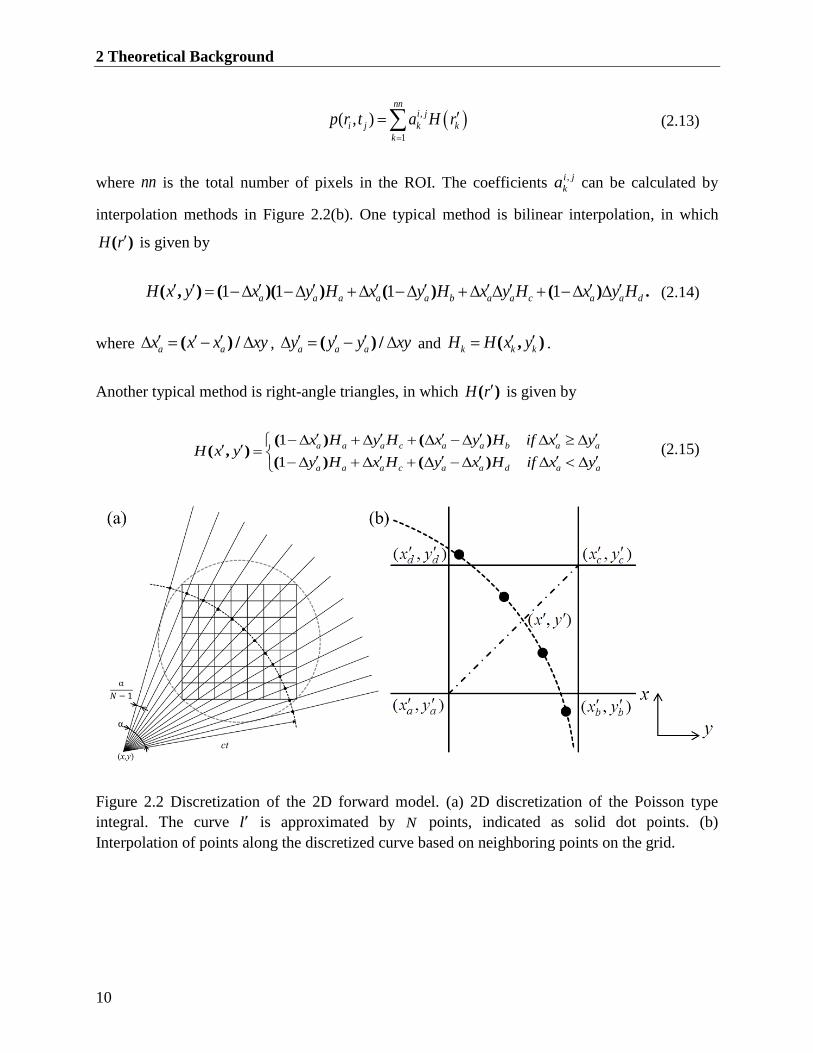
Figure 2.2 Discretization of the 2D forward model. (a) 2D discretization of the Poisson type
integral. The curve l is approximated by N points, indicated as solid dot points. (b)
Interpolation of points along the discretized curve based on neighboring points on the
grid. ................................................................................................................................... 10
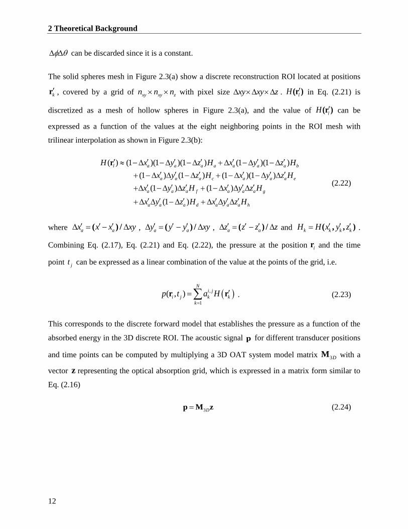
Figure 2.3 Discretization of the 3D forward model. (a) 3D discretization of the Poisson type
integral. The ROI mesh is shown as solid spheres; the discretized integral mesh, as
hollow spheres. (b) Trilinear interpolation with the eight neighboring points. ................ 13
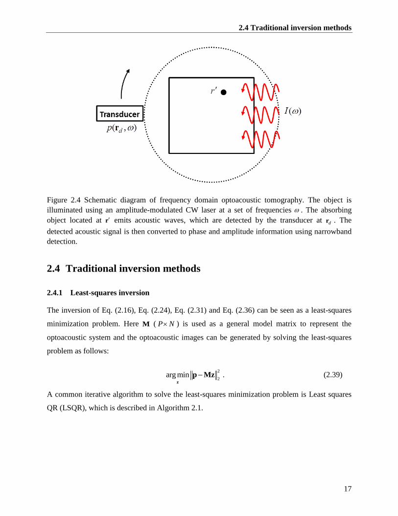
Figure 2.4 Schematic diagram of frequency domain optoacoustic tomography. The object is
illuminated using an amplitude-modulated CW laser at a set of frequencies . The
absorbing object located at r emits acoustic waves, which are detected by the transducer
at dr . The detected acoustic signal is then converted to phase and amplitude information
using narrowband detection. ............................................................................................. 17
Figure 3.1 Diagram of the optoacoustic tomography setup (a) Diagram of the optoacoustic
tomography setup. (b) Photograph of a single element transducer. .................................. 24
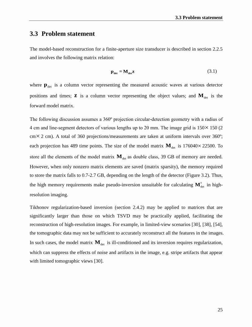
Figure 3.2 Amount of memory required to store the model matrix described in Sec. 2.2.5 when
sparsity is exploited (only non-zero entries are saved). The longer the detector is, the
more memory is required. Without sparsity, the matrix occupies 39 GB of memory.
(taken from [26]) ............................................................................................................... 26
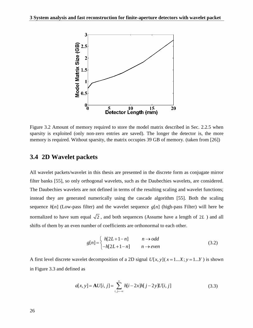
Figure 3.3 First level of 2D wavelet packet decomposition with scaling sequence and wavelet
sequence. ........................................................................................................................... 27
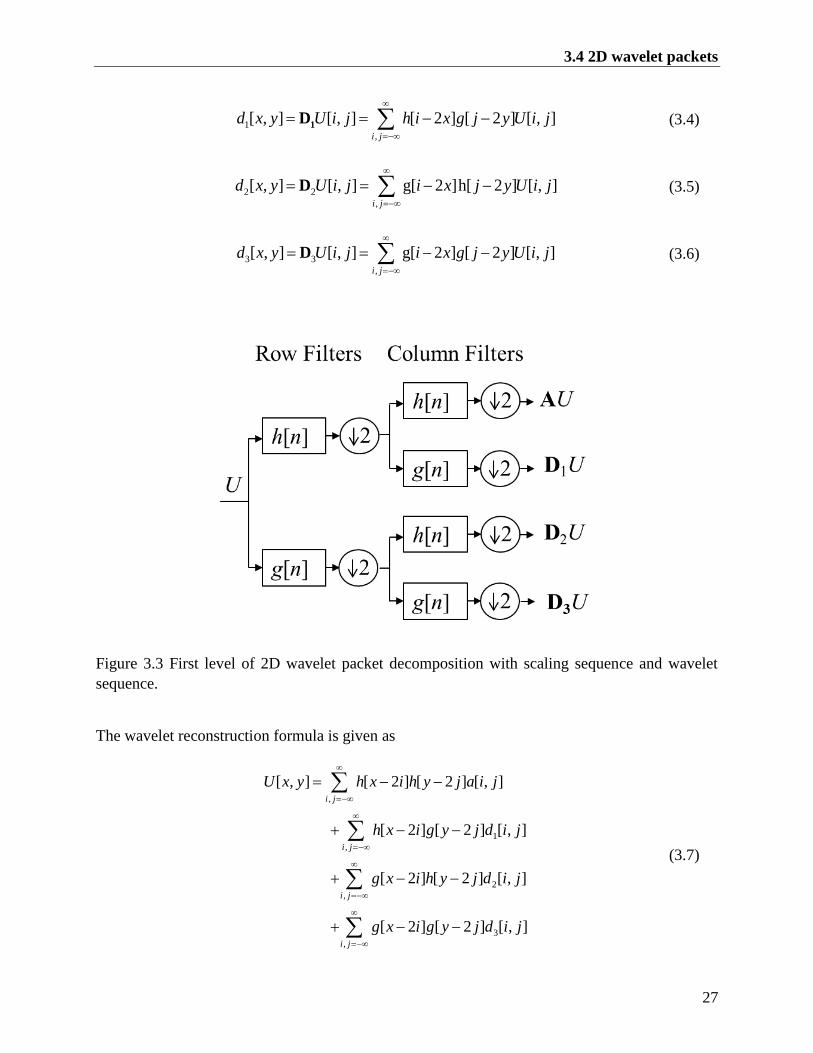
Figure 3.4 Full-tree 2D wavelet packet decomposition of level 2. ............................................... 28
Figure 3.5 Condition Number of the Model Matrix. (a) Map of decomposition components with
two-level wavelet packets. (b-d) Condition number map of the decomposed model matrix
List of Figures
XII
for a point detector, line detector 6 mm long, and line detector 13 mm long. (e) Maximum
condition number of all decomposition matrices with different detector lengths. (f)
Condition number of the model matrix with different detector lengths. (taken from [26])
........................................................................................................................................... 32
Figure 3.6 Optoacoustic signals detected from the sphere by detectors of various lengths. (a) The
image generated by the row in iV , which corresponds to the minimum singular value in
all the matrices i
wM calculated with a detector length of 6 mm. The result corresponds to
the image for which reconstruction is expected to show the greatest instability. (b) An
illustration of a spherical source with a radius of 200 µm positioned at the location
identified in panel (a). (c) The signals detected from the sphere by detectors of various
lengths and (d) their corresponding frequency content. (taken from [26]) ....................... 33
Figure 3.7 Evaluation of the reconstructions for numerical spheres phantoms in Table 3.1. (a)
Schematic illustration of a random object function. (b) Mean SSIM of random objects
with different detector lengths and regularization parameters. (c) Mean RMSD of random
objects with different detector lengths and regularization parameters. (d) Bias-variance
curve of the reconstructions for a point detector and for flat detectors with lengths of 1, 2,
3, 4, 5, 6, 8, 13, and 20 mm. Three values of α were considered (0, 0.05, and 0.1). For all
detector lengths, bias and variance were higher at α = 0 (no regularization) than at the
other α values. The worst bias and variance were obtained with a flat detector 4 mm long.
(taken from [26]) ............................................................................................................... 35
Figure 3.8 The numerical phantom used in the simulations. (taken from [26]) ........................... 37
Figure 3.9 Reconstructions of the numerical mouse phantom for the case of full-view, noisy data
using (a) BP, (b) IMMI, (c) IMMI-FAD, (d) GWP-IMMI-FAD. (e) Profiles of absorbed
energy density along the yellow dashed line in panel (c) for the original image and for
reconstructions prepared using IMMI-FAD or GWP-IMMI-FAD. (taken from [26]) ..... 40
Figure 3.10 Reconstructions of the numerical mouse phantom for the case of noisy, limited-view
data (projections spanning 180º on the left plane only) using (a) BP, (b) IMMI, (c) IMMI-
FAD, (d) GWP-IMMI-FAD and (e) WP-IMMI-FAD. (f) Profiles of absorbed energy
density along the yellow dashed line in panel (c) for the original image and for
reconstructions using IMMI-FAD or GWP-IMMI-FAD. (taken from [26]) .................... 41
List of Figures
XIII
Figure 3.11 Optoacoustic reconstructions of microspheres from experimental data using (a) BP,
(b) IMMI, (c) IMMI-FAD and (d) GWP-IMMI-FAD. (taken from [26]) ........................ 42
Figure 3.12 Optoacoustic reconstructions of a mouse brain from experimental data using (a) BP,
(b) IMMI, (c) IMMI-FAD and (d) GWP-IMMI-FAD. (taken from [26]) ........................ 43
Figure 3.13 Optoacoustic reconstructions of a mouse brain from limited-view (180º)
experimental data using (a) BP, (b) IMMI, (c) IMMI-FAD and (d) GWP-IMMI-FAD.
(taken from [26]) ............................................................................................................... 44
Figure 4.1 2D optoacoustic imaging system setup. (a) The schematic of the optoacoustic imaging
system setup. (b) Illumination and detection geometry in the imaging chamber. The
transducer can be translated along the z-axis in order to acquire multiple transverse cross
sections in the x–y plane. (taken from [64]) ..................................................................... 52
Figure 4.2 Detection geometries in the simulation and experiment in (a) nearly full-view and (b)
limited-view. (taken from [64]) ........................................................................................ 56
Figure 4.3 Simulation reconstructions in nearly full-view performed using (a) Tik-Lap, (b) TV,
(c) L1 and (d) TV-L1. (taken from [64]) .......................................................................... 57
Figure 4.4 Simulation reconstructions in limited-view performed using (a) Tik-Lap, (b) TV, (c)
L1 and (d) TV-L1. (taken from [64]) ................................................................................ 58
Figure 4.5 Reconstructed cross-sectional mouse images obtained from nearly full-view
projection data using (a) Tik-Lap, (b) TV, (c) L1 and (d) TV-L1. Yellow regions in
panels (a)-(d) are shown as zoomed images in panels (e)-(h). The FWHM values of the
vessel along the dashed line in panels (e)-(h) are compared in panel (i). (taken from [64])
........................................................................................................................................... 59
Figure 4.6 Reconstructed cross-sectional mouse images obtained from limited-view projection
data using (a) Tik-Lap, (b) TV, (c) L1 and (d) TV-L1. (taken from [64]) ....................... 60
Figure 5.1 Layout and color photograph of the hand-held MSOT probe for 3D imaging. (taken
from [78]) .......................................................................................................................... 67
Figure 5.2 Simulation results of the 3D optoacoustic imaging system. (a) 3D optoacoustic
tomography geometry tested in simulations and experiments. (b) Sketch of five spherical
absorbers with truncated parabolic absorption. (c) MIP results from the original data, and
reconstructions using BP, L2-LSQR, L1-GDBT or L1-GDBB at a noise level of 0 dB.
Reconstructions are shown in the x-y and y-z planes. (taken from [83]) ......................... 71
List of Figures
XIV
Figure 5.3 Comparison of convergence performance of simulated reconstructions at a noise level
of 0 dB using L2-LSQR, L1-GDBT or L1-GDBB. Variations in RMSD and objective
function are depicted as a function of (a-b) iteration number and (c-d) CPU time. (taken
from [83]) .......................................................................................................................... 72
Figure 5.4 Single slices of original data and reconstructions generated using BP, L2-LSQR, L1-
GDBT or L1-GDBB at a noise level of 0 dB. (a) z=0 plane (top row) and y=0 plane
(bottom row). (b) Line profiles of the original data and four reconstructions along Line 1
in (a). (taken from [83]) .................................................................................................... 73
Figure 5.5 Reconstructions of experimental data using BP, L2-LSQR, L1-GDBT and L1-GDBB.
(a-b) MIP results (side and top views) of reconstructions of experimental data using BP,
L2-LSQR, L1-GDBT and L1-GDBB. (c) Zoomed-in images of the top-view MIP region
enclosed in the dot-dashed box in (b). The corresponding region for each reconstruction
is shown, even though the box is drawn only for BP. The regions labeled “T” and “B”
served as target and background regions, respectively, for calculating SNR and CNR.
(taken from [83]) ............................................................................................................... 75
Figure 6.1 Projection parameters that influence FD-OAT reconstruction. (a) Detection geometry.
(b) One full phase cycle is needed to uniquely differentiate each pixel. .......................... 79
Figure 6.2. FD-OAT geometry in the frequency domain. maxk is the largest angular spacing
between two neighboring projections, rk is the radial sampling interval,
maxf is the
maximum frequency and c is the speed of sound. ........................................................... 80
Figure 6.3 Validation of the predicted minimum number of projections needed to avoid aliasing
artifacts during FD-OAT reconstruction. (a) Original image. (b-d) Reconstructions with
projection numbers equal to 20%, 50% or 100% of the required projections at the
modulation frequency of 2.6 MHz and reconstruction dimension of 12 mm. (e) Criterion
as a function of projection number. (f) Maximum intensity of the reconstruction as a
function of projection number. ......................................................................................... 82
Figure 6.4 (a) Map of the logarithm of condition number (CN) as a function of different numbers
of projections and modulation frequencies. (b) Map of the ratio of total measurements to
total pixels as a function of different numbers of projections and modulation frequencies.
........................................................................................................................................... 84
XV
List of Tables
Table 3.1 Parameters of 9 spheres to generate 100 random numerical phantoms. (taken from [26])
....................................................................................................................................................... 34
Table 4.1 Regularization parameters used during reconstructions. (taken from [64]) ................. 61
Table 4.2 Iteration number and processing time for reconstructions. (taken from [64]) .............. 61
Table 4.3 Quantitative evaluation of reconstructions. (taken from [64]) ..................................... 62

List of Tables
XVI
XVII
List of abbreviations
CW
OAT
2D
3D
TSVD
MSOT
ROI
SIR
LSQR
SVD
BP
IMMI
WP
WP-IMMI
FAD
IMMI-FAD
GWP-IMMI-FAD
RAM
STD
Continuous-wave
Optoacoustic tomography
Two-dimensional
Three-dimensional
Transacted singular value decomposition
Multispectral optoacoustic tomography
Region of interest
Spatial impulse response
Least squares QR
Singular value decomposition
Back-projection
Interpolated-model-matrix-inversion
Wavelet-packet
Wavelet-packet domain based interpolated-model-matrix-inversion
Finite-aperture detectors
Interpolated-model-matrix-inversion with finite-aperture detectors
Generalized wavelet-packet based interpolated-model-matrix-inversion
Random access memory
Standard deviation
List of Abbreviations
XVIII
RMSD
SSIM
TV
TV-L1
Tik-Lap
OPO
SNR
CNR
L1-GDBB
L1-GDBT
L2-LSQR
UTA
GPU
FD-OAT
TD-OAT
ES
Tik
Root-mean-square-deviation
Structural similarity
Total variation
Total variation and L1 norm based inversion
Tikhonov regularization with a Laplacian penalty
Optical parametric oscillator
Signal-to-noise ratio
Contrast-to-noise ratio
Sparsity-based inversion using gradient descent & Barzilai-Borwein line search
Sparsity-based inversion using gradient descent & backtracking line search
LSQR algorithm with L2-norm regularization
Ultrasound transducer array
Graphics processing unit
Frequency domain optoacoustic tomography
Time domain optoacoustic tomography
Even sampling
Tikhonov
1
1 Introduction
1.1 Optoacoustic imaging
Optoacoustic imaging, also termed photoacoustic imaging, is a noninvasive imaging technique
that holds great promise for clinical or preclinical applications [1]–[5]. Optoacoustic imaging is a
hybrid imaging modality that is capable of visualizing optical contrast at imaging depths and
resolutions often found in medical ultrasonography [6]. Optoacoustic imaging can be regarded as
an ultrasound modality that exploits optical-absorption image contrast, which can give deeper
information than pure optical imaging [1]. With this advantage, numerous fundamental studies of
optoacoustic imaging on theory, instruments and applications have been investigated in recent
years [1]–[5].
A typical optoacoustic imaging system employs a laser to illuminate the object, and the acoustic
signals generated by the optoacoustic effect then propagate from the inside of the object and can
be measured by ultrasonic transducers outside of the object [7]–[9]. The optoacoustic image of
the object corresponds to the optical energy deposition (light absorption) in the object [10].
Optoacoustic imaging can also be classified into two categories: optoacoustic
microscopy/mesoscopy [11], [12] and optoacoustic tomography [13], [14]. Optoacoustic
microscopy usually employs mechanical raster scanning of a high-frequency focused transducer
(in the case of acoustic resolution optoacoustic microscopy) or a focused laser beam (in the case
of optical resolution optoacoustic microscopy) in order to acquire the acoustic signals. In these
cases, the optoacoustic image is obtained from the set of A-lines and requires no reconstruction
algorithms. Optoacoustic mesoscopic imaging also is performed in similar lines, just that the
ultrasound will be operating at frequency range of tens of MHz. Optoacoustic tomography, in
contrast, generally illuminates the object over a broad range, and the acoustic signals are
1 Introduction
2
acquired by mechanically scanning with a low-frequency transducer or an array of detectors.
Then this acoustic data is provided to a reconstruction algorithm to generate the optoacoustic
image. There are three commonly used detection geometries in optoacoustic tomography:
spherical, cylindrical and planar. The cylindrical and spherical detection geometries require
collecting all the measurements around the target, while the planar detection geometry allows
more flexibility about where measurements can be acquired.
Optoacoustic imaging can be presented using the time domain methodology [15] or frequency
domain methodology [16], [17] depending on the laser employed. The classic time domain
optoacoustic imaging methodology employs a short-pulse (nanosecond range), high peak-power
laser for illumination, while frequency domain optoacoustic imaging uses a periodic, intensity-
modulated, continuous-wave (CW) laser.
1.2 Reconstructions in optoacoustic imaging
Most optoacoustic tomography reconstruction algorithms are based only on the acoustic wave
equation, modeling the propagation of optoacoustically generated acoustic waves [10], [18]. The
“forward problem” in optoacoustic tomography refers to the process in which light energy
deposited at optical absorbers is converted to ultrasonic pressure waves. Image reconstruction in
optoacoustic tomography can then be considered the “inverse” of the forward problem:
calculating the optoacoustic images from the recorded pressure signals [19]–[25].
For an optoacoustic tomography system with specific transducer and detection trajectory, image
reconstruction can be performed either analytically or numerically. Various analytic optoacoustic
tomography reconstruction algorithms such as back-projection methods and time reversal
methods have been developed for optoacoustic tomography under the assumption of point-like
ultrasound transducers [19]–[21], [23]. This may lead to reconstruction inaccuracies and artifacts,
e.g. in systems with large-area acoustic detectors [26]–[29]. In addition, analytic optoacoustic
tomography reconstruction algorithms have a closed-form solution and are numerically stable
only when the measurement aperture encloses the entire object, which is not feasible in many
clinical or pre-clinical optoacoustic tomography applications with limited-view geometries [30],
[31]. Numerical model-based optoacoustic tomography reconstruction algorithms represent a
1.3 Goals and objectives
3
potent alternative to the analytic approaches because they can more generally account for
system- and geometry-related parameters [20], [24], [26] , [29]–[35]. Optoacoustic tomography
reconstructions based on models in the time domain [24], [27], [32]–[35] or frequency domain
[36], [37] can model any additional physical effects, such as acoustic heterogeneities and
attenuation, light propagation or geometric detector properties. Despite the accurate performance
achieved by model-based reconstructions algorithms, one of the main disadvantages is their
computational complexity and need for computer memory, especially in the case of finite-size
detectors or with more pixels [26]. Normally a more complex model leads to a more accurate
reconstruction, but a large optoacoustic tomography model matrix will lead to excessive
reconstruction times.
1.3 Goals and objectives
The goals of this dissertation are to develop and implement various fast and accurate model-
based reconstruction methods for different optoacoustic tomography (OAT) systems: a 2D OAT
system with a finite-size single element transducer; a 2D OAT system with cylindrically focused
curved arrays; and a 3D OAT system with spherically focused, curved arrays. Accurate image
reconstruction improves not only the visualization of anatomical results, but it also facilitates
subsequent multispectral analysis for oxygen saturation, molecular targeting, and other
applications. A key consideration in developing these reconstruction methods is the way to build
the optoacoustic forward model matrix, and the manner to achieve fast and accurate results with
acoustic inversion. This dissertation also examines the relationship among spatial resolution,
frequency and projection number in order to guide the set-up of a frequency domain OAT; this
approach can also be applied to time domain OAT.
1.4 Outline of the Thesis
The dissertation is structured as follows. Chapter 2 provides the reader with theoretical
background on optoacoustic imaging in the time and frequency domains; key concepts include
optoacoustic signal generation, the optoacoustic wave equation, the forward solution of the
optoacoustic wave equation and the forward matrix. Common inversion methods such as
transacted singular value decomposition and Tikhonov regularization are also introduced. In
1 Introduction
4
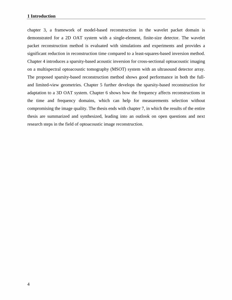
chapter 3, a framework of model-based reconstruction in the wavelet packet domain is
demonstrated for a 2D OAT system with a single-element, finite-size detector. The wavelet
packet reconstruction method is evaluated with simulations and experiments and provides a
significant reduction in reconstruction time compared to a least-squares-based inversion method.
Chapter 4 introduces a sparsity-based acoustic inversion for cross-sectional optoacoustic imaging
on a multispectral optoacoustic tomography (MSOT) system with an ultrasound detector array.
The proposed sparsity-based reconstruction method shows good performance in both the full-
and limited-view geometries. Chapter 5 further develops the sparsity-based reconstruction for
adaptation to a 3D OAT system. Chapter 6 shows how the frequency affects reconstructions in
the time and frequency domains, which can help for measurements selection without
compromising the image quality. The thesis ends with chapter 7, in which the results of the entire
thesis are summarized and synthesized, leading into an outlook on open questions and next
research steps in the field of optoacoustic image reconstruction.
5
2 Theoretical Background
This chapter first presents a short introduction to the fundamental principles of optoacoustic
imaging. Furthermore, key concepts about optoacoustic signal generation, the forward solution
and modeling the optoacoustic effect are given in the time domain (section 2.2) and frequency
domain (section 2.3). The concepts in this chapter provide a theoretical background for
understanding the technical details, simulations, experiments and discussions in subsequent
chapters.
2.1 Optoacoustic principles
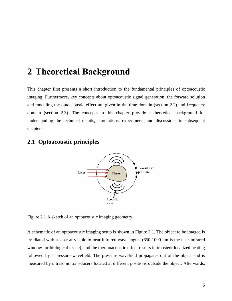
Figure 2.1 A sketch of an optoacoustic imaging geometry.
A schematic of an optoacoustic imaging setup is shown in Figure 2.1. The object to be imaged is
irradiated with a laser at visible to near-infrared wavelengths (650-1000 nm is the near-infrared
window for biological tissue), and the thermoacoustic effect results in transient localized heating
followed by a pressure wavefield. The pressure wavefield propagates out of the object and is
measured by ultrasonic transducers located at different positions outside the object. Afterwards,
2 Theoretical Background
6
image reconstruction algorithms can recover the initial distribution of optical energy deposited
within the object, which is dependent on the illumination and the optical properties of the object.
Two types of laser illumination can be used to generate optoacoustic signals: short (nanosecond)
optical pulses with high peak power, or modulated CW lasers with relatively low mean power
and high modulation frequency. These two categories will be described in detail in the next two
sections.
2.2 Time domain optoacoustic imaging
2.2.1 Optoacoustic signal generation and wave equation in time domain
In order to achieve good spatial resolution for time domain optoacoustic imaging, two
confinements should be fulfilled [3], [5]. One confinement is thermal confinement, which means
the laser pulse width p needs to be much shorter than thermal confinement th in order to avoid
thermal diffusion:
2
4
cp th
T
d
D , (2.1)
where cd is the characteristic dimension (targeted spatial resolution) and T
D is the thermal
diffusivity (a typical value for most soft tissues is 5 21.4 10 /mm s ) [39]. With a 10-
nanosecond pulse laser, the best spatial resolution guided by thermal confinement is ~0.06 m ,
which is much less than the spatial resolution of optoacoustic imaging. Another confinement is
acoustic stress confinement, which means that optoacoustic propagation of the absorber during
laser illumination is negligible:
cp s
d
c , (2.2)
where c is the speed of sound. With a 10-nanosecond pulse laser and c of 1500 /m s (typical
for biological tissue) [40], the best spatial resolution guided by acoustic stress confinement is
~15 m .
2.2 Time domain optoacoustic imaging
7
Under these two confinements, the initially induced in optoacoustic wave pressure 0p r within
the tissue is [5]
2
0 p ap c C H r / r r r (2.3)
where is the thermal expansion coefficient ( 1K ), pC is the heat capacity ( / (kg K)J • ),r is
the position, a r is the optical absorption coefficient (
1cm), r is the optical fluence
(2/J cm ), is the Grueneisen parameter, which equals 2
pc C / and represents the amount of
temperature converted to optoacoustic pressure and H r is the absorbed optical energy, which
equals a r r .
Optoacoustic wave generation and propagation in an acoustically homogeneous medium is
described by the following optoacoustic equation [41]
2
2 2
2
( , ) ( , )- ( , )
p t H tc p t
t t
r rr (2.4)
where t is time, r is the position in 3D space, ( , )p tr is the generated pressure, is the
Grueneisen parameter, and ( , )H tr is the amount of energy absorbed in the tissue per unit
volume and per unit time. If ( , )H tr can be separated into spatial and temporal components, then
Eq. (2.4) can be simplified as:
22 2
2
( )( , )- ( , ) ( ) t
r
H tp tc p t H
t t
rr r (2.5)
where ( )rH r and ( )tH t are, respectively, the energy per unit volume and energy per unit time.
When the laser pulse is short enough to satisfy the acoustic stress confinement, ( )tH t can be
approximated by a delta function.
2 Theoretical Background
8
2.2.2 Forward solution of optoacoustic wave equation in time domain
The optoacoustic equation in Eq. (2.5) can be solved using Green’s function [42], which
describes the profile of generated optoacoustic signal, when spatial and temporal impulse source
is used:
2
2
2 2
1G t t t t
c t
r, ;r , r r , (2.6)
where r is the source location and t is the time. Green’s function can be solved as
4
t t cG t t
r r /r, ;r ,
r r. (2.7)
With the Green’s function in Eq. (2.7) and the optoacoustic wave equation in Eq. (2.4), we can
obtain the pressure due to an arbitrary source in an infinite medium:
/2
( )( , ) ( )
4
rt t c
Hp t H t d
c t
r r
rr r
r r (2.8)
A widely used optoacoustic time domain inversion formula is the universal back-projection (BP)
algorithm [19], which has been analytically inverted from Eq. (2.8) for different detection
geometries. The approximate analytical solution is given by [19]
2 2r t c
p tH r p t t dr
t
'
'
' '
r r /
r ,r , (2.9)
The back-projection algorithm is successful in detecting the position and shape of absorbing
objects, even though Eq. (2.9) is not the exact solution [24]. However, this algorithm has several
drawbacks. First, t p t t p t ' 'r , / r , exists in most cases (far-field acoustic detection) and
the derivative part implies a ramp filter, which will enhance the boundaries and impair the low-
frequency information in back-projection reconstruction. Second, negative values without
physical meaning often appear in the reconstruction. Third, the algorithm cannot take detector
2.2 Time domain optoacoustic imaging
9
response into account. This highlights the need for model-based reconstructions for quantitative
image reconstruction, which will be discussed in the following sections.
2.2.3 Time domain 2D forward modeling
The 2D time domain forward modeling used in this dissertation is based on discretization of Eq.
(2.8) as described previously [35]. First, Eq. (2.8) is approximated as
2
I t t I t tp t
t
r, (2.10)
where
r
t cl
HI t dl
r r' /
(r )
r r (2.11)
Eq. (2.11) is discretized by approximating the curve at a distance of l ct from the transducer’s
position and with N straight lines (Figure 2.2(a)). This set of straight lines covers an angle of
2arcsin 2 1 / 2n xy R , where n is the pixel number in the x and y directions,
xy is the pixel size and R is the distance from the transducer to the center of the region of
interest (ROI).
The integral I t is then calculated from N discrete points of the curve l with positions lr
(solid dots in Figure 2.2(a)) as
1, , 1
1
( )1( )
2
Nl
l l l l
l l
HI t d d
r
r r (2.12)
where 0,1 , 1 0N Nd d . ( )lH r is estimated by interpolating ( )H r at pixel positions in the ROI.
Combining Eq. (2.10) and Eq. (2.12), the pressure ( , )i jp tr measured at position ir and time jt
can be expressed as a linear combination of the absorbed energy at pixel position kr in the ROI:
2 Theoretical Background
10
,
1
( , )nn
i j
i j k k
k
p r t a H r
(2.13)
where nn is the total number of pixels in the ROI. The coefficients ,i j
ka can be calculated by
interpolation methods in Figure 2.2(b). One typical method is bilinear interpolation, in which
H r( ) is given by
1 1 1 1a a a a a b a a c a a d
H x y x y H x y H x y H x y H ( , ) ( )( ) ( ) ( ) . (2.14)
where a ax x x xy ( ) / , a a a
y y y xy ( ) / and k k kH H x y ( , ) .
Another typical method is right-angle triangles, in which H r( ) is given by
1
1
a a a c a a b a a
a a a c a a d a a
x H y H x y H if x yH x y
y H x H y x H if x y
( ) ( )( , )
( ) ( ) (2.15)
Figure 2.2 Discretization of the 2D forward model. (a) 2D discretization of the Poisson type
integral. The curve l is approximated by N points, indicated as solid dot points. (b)
Interpolation of points along the discretized curve based on neighboring points on the grid.
2.2 Time domain optoacoustic imaging
11
When the pressure in Eq. (2.13) is computed for P transducer positions and for I time points, a
linear equation can be formulated to express the transform from the image z (optical absorption)
to the acoustic signals p by a model matrix 2DM , which represents a 2D OAT system
2Dp M z (2.16)
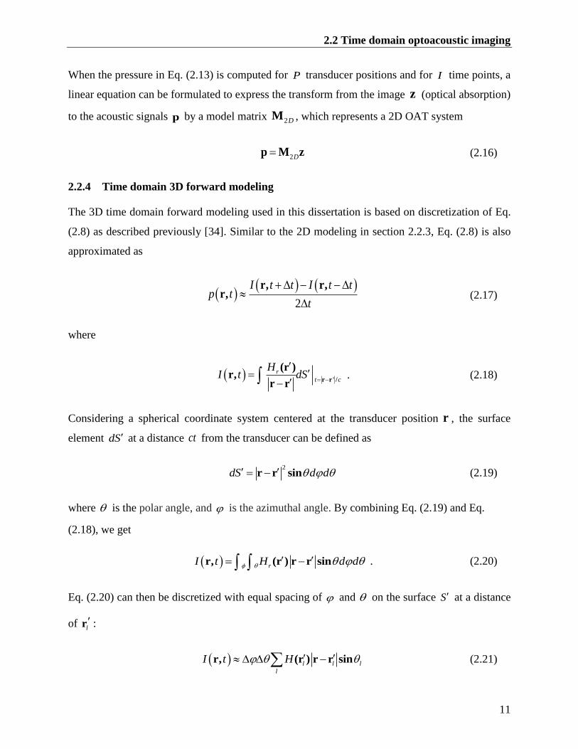
2.2.4 Time domain 3D forward modeling
The 3D time domain forward modeling used in this dissertation is based on discretization of Eq.
(2.8) as described previously [34]. Similar to the 2D modeling in section 2.2.3, Eq. (2.8) is also
approximated as
2
I t t I t tp t
t
r, r,r, (2.17)
where
r
t c
HI t dS
r r' /
(r )r,
r r . (2.18)
Considering a spherical coordinate system centered at the transducer position r , the surface
element dS at a distance ct from the transducer can be defined as
2
dS d d r r sin (2.19)
where is the polar angle, and is the azimuthal angle. By combining Eq. (2.19) and Eq.
(2.18), we get
rI t H d d r, (r ) r r sin . (2.20)
Eq. (2.20) can then be discretized with equal spacing of and on the surface S at a distance
of lr :
l l l
l
I t H r, (r ) r r sin (2.21)
2 Theoretical Background
12
can be discarded since it is a constant.
The solid spheres mesh in Figure 2.3(a) show a discrete reconstruction ROI located at positions
kr , covered by a grid of xy xy zn n n with pixel size xy xy z . l
H (r ) in Eq. (2.21) is
discretized as a mesh of hollow spheres in Figure 2.3(a), and the value of lH (r ) can be
expressed as a function of the values at the eight neighboring points in the ROI mesh with
trilinear interpolation as shown in Figure 2.3(b):
( ) (1 )(1 )(1 ) (1 )(1 )
(1 ) (1 ) (1 )(1 )
(1 ) (1 )
(1 )
l a a a a a a a b
a a a c a a a e
a a a f a a a g
a a a d a a a h
H x y z H x y z H
x y z H x y z H
x y z H x y z H
x y z H x y z H
r
(2.22)
where a ax x x xy ( ) / , a a
y y y xy ( ) / , a az z z z ( ) / and k k k k
H H x y z ( , , ) .
Combining Eq. (2.17), Eq. (2.21) and Eq. (2.22), the pressure at the position ir and the time
point jt can be expressed as a linear combination of the value at the points of the grid, i.e.
,
1
( , )N
i j
i j k k
k
p t a H
r r . (2.23)
This corresponds to the discrete forward model that establishes the pressure as a function of the
absorbed energy in the 3D discrete ROI. The acoustic signal p for different transducer positions
and time points can be computed by multiplying a 3D OAT system model matrix 3DM with a
vector z representing the optical absorption grid, which is expressed in a matrix form similar to
Eq. (2.16)
3Dp M z (2.24)
2.2 Time domain optoacoustic imaging
13
Figure 2.3 Discretization of the 3D forward model. (a) 3D discretization of the Poisson type
integral. The ROI mesh is shown as solid spheres; the discretized integral mesh, as hollow
spheres. (b) Trilinear interpolation with the eight neighboring points.
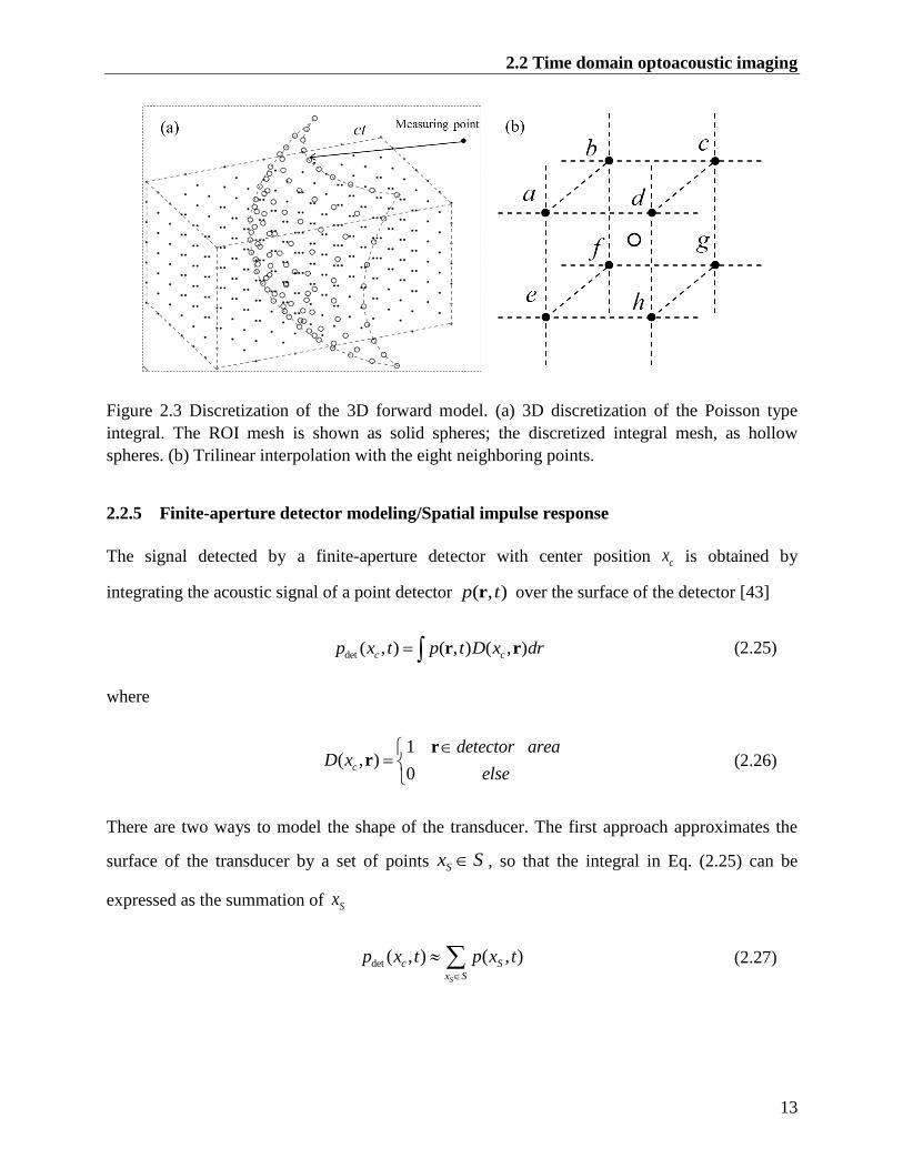
2.2.5 Finite-aperture detector modeling/Spatial impulse response
The signal detected by a finite-aperture detector with center position cx is obtained by
integrating the acoustic signal of a point detector ( , )p tr over the surface of the detector [43]
det ( , ) ( , ) ( , )c cp x t p t D x dr r r (2.25)
where
1
( , )0
c
detector areaD x
else
rr (2.26)
There are two ways to model the shape of the transducer. The first approach approximates the
surface of the transducer by a set of points Sx S , so that the integral in Eq. (2.25) can be
expressed as the summation of Sx
det ( , ) ( , )S
c S
x S
p x t p x t
(2.27)
2 Theoretical Background
14
The pressure ( , )Sp x t for a point detector has been studied in Eq. (2.16), and assuming linearity,
the model matrix sumM , which takes into account the effects of the finite-size transducer, can
also be summed with the model matrices of individual points Sx S :
S
S
sum x
x S
M M (2.28)
such that the signal acquired by the transducer for a set of time points and transducer locations
can be expressed as
det sump M z (2.29)
The accuracy of this procedure depends on the number of points used to discretize the detector
shape, and this method has the flexibility to model any detector shape. Its only drawback is that
it is slow for large detectors.
An alternative way to calculate det ( , )cp x t is the convolution the spatial impulse response (SIR)
of a finite length line transducer with the optoacoustic wave ( , )p tr in Eq. (2.8) [27]:
det /2
( , ) ( )( , )
4
c rc t c
D x Hp x t dr
c t
r r
r r
r r (2.30)
where c is the speed of sound in the medium, is the Grueneisen parameter, ( )rH r is the
amount of energy absorbed in the tissue per unit volume, and * denotes the spatial convolution
operator. The discretization of Eq. (2.30) can be expressed as the following linear relation:
det detp M z (2.31)
In the case of a long line transducer where a lot of points would be needed to approximate the
line for calculating the sumM , then model matrix detM is preferable since it can be calculated
much quicker.
2.3 Frequency domain optoacoustic imaging
15
2.3 Frequency domain optoacoustic imaging
2.3.1 Optoacoustic signal generation and wave equation in frequency domain
Analogous to the situation in time domain optoacoustic imaging, thermal and acoustic stress
confinement in frequency domain optoacoustic imaging are governed by two characteristic
frequencies, th and s , which are the inverses of the corresponding characteristic times th and
s in Eqs. (2.1) and (2.2):
2
41 Tt
th c
D
d
(2.32)
1
ss c
c
d
(2.33)
where cd is the characteristic dimension (targeted spatial resolution) and T
D is the thermal
diffusivity and c is the speed of sound.
Under conditions of heat and acoustic stress confinement, the generation and propagation of
frequency domain acoustic waves can be described by the following Helmholtz equation [37]
2 2
p
ip k p H
C
r, r, r, (2.34)
where r is the position, is the angular frequency, p r, is the Fourier transform of the
acoustic pressure wave, /k c is the acoustic wave number, 1i , is the thermal
expansion coefficient, pC is the specific heat capacity, and H r, is the Fourier transform of
the absorbing source.
2.3.2 Forward solution of optoacoustic wave equation in frequency domain
Green’s function for a source in an unbounded medium has the solution [16]
4
ik
p
i ep H dr
C
r r
r, r ,r r
(2.35)
2 Theoretical Background
16
where r is the source location.
2.3.3 Frequency domain 2D forward modeling
A schematic of frequency domain optoacoustic tomography is shown in Figure 2.4. The
transducer scans 360° around the sample with P projections located at dr . The sample area is
discretized as a square grid with pixel size d and N pixel nodes. Assuming an infinite and
homogeneous medium, the pressure wave located at position r is given by the Green’s function
solution in Eq. (2.35). Accordingly, the pressure ( , )dp r at position dr and modulation
frequency can be given by the linear expression
( ) ( ) p M z (2.36)
where ( )p is a complex column vector denoting the measured complex signals (amplitude and
phase of the pressure wave) at P projection positions, and z is a real vector representing the
unknown absorption. ( )M is a complex matrix of dimensions P N :
11 1
1
( ) a
n
i
P PN
m m
iAe
m m
M (2.37)
where
( ( ( ) ( ) / ))
( ) ( )
di n p c
pn
d
em
n p
r r
r r (2.38)
and where ( )d pr denotes the p th detector position, ( )nr is the position of voxel n and A is a
constant.
2.4 Traditional inversion methods
17
Figure 2.4 Schematic diagram of frequency domain optoacoustic tomography. The object is
illuminated using an amplitude-modulated CW laser at a set of frequencies . The absorbing
object located at r emits acoustic waves, which are detected by the transducer at dr . The
detected acoustic signal is then converted to phase and amplitude information using narrowband
detection.
2.4 Traditional inversion methods
2.4.1 Least-squares inversion
The inversion of Eq. (2.16), Eq. (2.24), Eq. (2.31) and Eq. (2.36) can be seen as a least-squares
minimization problem. Here M ( P N ) is used as a general model matrix to represent the
optoacoustic system and the optoacoustic images can be generated by solving the least-squares
problem as follows:
2
2arg min
z
p Mz . (2.39)
A common iterative algorithm to solve the least-squares minimization problem is Least squares
QR (LSQR), which is described in Algorithm 2.1.
2 Theoretical Background
18
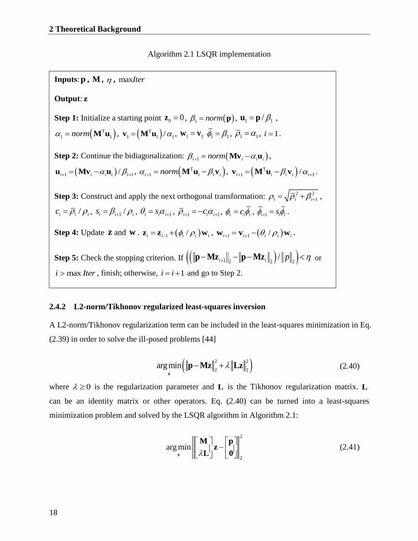
Algorithm 2.1 LSQR implementation
2.4.2 L2-norm/Tikhonov regularized least-squares inversion
A L2-norm/Tikhonov regularization term can be included in the least-squares minimization in Eq.
(2.39) in order to solve the ill-posed problems [44]
2 2
2 2arg min
z
p Mz Lz (2.40)
where 0 is the regularization parameter and L is the Tikhonov regularization matrix. L
can be an identity matrix or other operators. Eq. (2.40) can be turned into a least-squares
minimization problem and solved by the LSQR algorithm in Algorithm 2.1:
2
2
arg min
z
M pz
L 0 (2.41)
Inputs:p , M , , maxIter
Output: z
Step 1: Initialize a starting point 0 0z , 1 norm p , 1 1/ u p ,
T
1 1norm M u , T
1 1 1/v M u , 1 1w v 1 1 , 1 1 , 1i .
Step 2: Continue the bidiagonalization: 1i i i inorm Mv u ,
1 1/i i i i i u Mv u , T
1i i i inorm M u v , T
1 1/i i i i i v M u v .
Step 3: Construct and apply the next orthogonal transformation: 2 2
1i i i ,
/i i ic , 1 /i i is , 1i i is , 1 1i i ic , i i ic , 1i i is .
Step 4: Update z and w . 1 /i i i i i z z w , 1 1 /i i i i i w v w .
Step 5: Check the stopping criterion. If 1 2 2 2/i i p p Mz p Mz or
maxi Iter , finish; otherwise, 1i i and go to Step 2.

2.4 Traditional inversion methods
19
2.4.3 Moore-Penrose pseudo-inversion with truncated singular value decomposition
Singular value decomposition (SVD) is a factorization of a real or complex matrix. SVD of a
matrix M can be formed as
T
M = UΣV (2.42)
where U is a m m unitary matrix, is a diagonal m n matrix with non-negative real
numbers on the diagonal representing singular values, T denotes the transpose operation, and
TV is an n n unitary matrix.
1 2( , ,..., )ndiag (2.43)
where 1 2 1... ... 0r r n and ( )r rank M .
The goal of truncated singular value decomposition (TSVD) and Tikhonov regularization is to
dampen the contributions from errors in measurement p (noise). TSVD is achieved by
neglecting the components of the solution corresponding to the partial smallest singular values,
since these are likely to contribute heavily to the solution. Thus, the TSVD of M is defined as
the rank- k matrix.
T T
11
, ,..., ,0,...,0k
m n
k k i i i k ki
u v diag R
M UΣ V Σ (2.44)
where k r , iu and iv are the columns of the matrices U and V , respectively. When k is
chosen properly, the condition number of kM ( 1 / k ) will be small. The TSVD solution to Eq.
(2.39) is defined by:
k
z M p . (2.45)
The pseudo-inverse matrix k
M is:
T 1 1
1, ,..., ,0,...,0 n m
k k k kdiag R M VΣ U Σ . (2.46)
The advantage of this approach is that the pseudo-inverse matrix may be pre-calculated for a
given system and then simply reapplied to each new dataset, thus reducing the image
reconstruction problem to a matrix-vector multiplication operation. The drawback of this
approach is that it is impartial to apply SVD decomposition when the matrix is too big.
2 Theoretical Background
20
2.4.4 L-curve method for selection of the regularization parameter
The L-curve is a log-log plot of the norm of a regularized component versus the norm of the
corresponding residual norm, since the regularization parameter varies [44]. The L-curve can
give insight into the regularizing properties of the underlying regularization method, and it is an
aid to choose an appropriate regularization parameter for the given data and regularization
method.
If too much regularization is imposed on the solution, it will not fit the given data p properly
and the residual norm 2 Mz p will be too large (where z is the regularized solution with
regularization parameter ). On the other hand, if too little regularization is imposed, then
2 Mz p will be good but the regularization part will be too large. Here we use Tikhonov
regularization as an example to explain the L-curve.
The ‘best’ regularization parameter λ lies in a more or less distinct corner of the L-curve
2 2log , log Mz p Lz . This corner separates the flat part of the curve where regularization
errors dominate, from the vertical part of the curve where noise dominates. At this corner the
curvature of the L-curve is maximal.
21
3 System analysis and fast reconstruction for
finite-aperture detectors with wavelet
packet
Optoacoustic tomography employs relatively large detectors to achieve high detection sensitivity.
Spatial-averaging effects over large detector areas may lead to attenuation of high acoustic
frequencies and, subsequently, loss of fine features in the reconstructed image. Model-based
reconstruction algorithms improve image resolution in such cases by correcting for the effect of
the detector’s aperture on the detected signals. However, the incorporation of the detector’s
geometry in the optoacoustic model significantly increases the amount of memory needed for
model matrix, which hinders the application of inversion and analysis tools such as singular
value decomposition. In this chapter we demonstrate the use of the wavelet-packet framework
for optoacoustic systems with finite-aperture detectors. The decomposition of the model matrix
in the wavelet-packet domain leads to model matrices sufficiently small to apply SVD. This
methodology is demonstrated to reduce inversion time more than 10-fold for simulated and
experimental data. In addition, the proposed framework for assessing inversion stability is
demonstrated, which reveals a non-monotonic dependency of the system condition number on
detector size, which has not been reported before. Thus, the proposed framework may assist in
choosing the optimal detector size in future optoacoustic systems.
Some of the material in this chapter has been presented in the following publication in a very
similar or identical form to the text in this chapter:
3 System analysis and fast reconstruction for finite-aperture detectors with wavelet packet
22
“Optoacoustic imaging reconstruction and system analysis method for finite-aperture detectors
under the wavelet-packet framework” by Yiyong Han, Vasilis Ntziachristos and Amir Rosenthal,
Journal of Biomedical Optics, 21(1), 016002, 2016.
3.1 Introduction
One of the commonly used classes of algorithms for optoacoustic image formation is the back-
projection (BP) reconstruction [19]. Despite their ubiquity, BP algorithms reflect an ideal
representation of the optoacoustic problem and are exact only in a few imaging geometries that
involve point-like detectors, which will generate reconstruction inaccuracies and artifacts in
systems with finite-aperture detectors. Model-based reconstruction algorithms represent a potent
alternative to the BP approaches owing to their generality in accounting for system- and
geometry-related parameters [24], [29], [45]–[47]. For instance, model-based algorithms have
succeeded in accounting for the effects of a detectors’ aperture and limited projection geometry
[27], [30], [38]. In the model-based approach implemented in this dissertation, termed
interpolated-model-matrix-inversion (IMMI), the model matrix that describes the optoacoustic
imaging system can be pre-calculated in advance for analysis and can easily undergo algebraic
inversion to accelerate the reconstruction [27], [46].
The main disadvantage of model-based reconstruction algorithms is their high computational
cost in terms of complexity and memory; this cost scales nonlinearly with the number of
reconstructed image pixels. The use of computationally expensive inversion algorithms such as
SVD therefore often limits the reconstruction grid to low resolution. Although IMMI is now
commonly employed in 2D OAT inversions [48], [49], the lengthy computational times have
restricted the widespread use of model-based approaches and make them unsuitable, for example,
in real-time MSOT applications [50] or 3D problems [38], [51].
Recently, a wavelet-packet (WP) framework was introduced to reduce the computational
demands of model-based reconstruction algorithms [52]. The use of wavelet packets enables the
decomposition of the model matrix into significantly smaller matrices, each corresponding to a
different spatial frequency band in the image. Inversion is thus performed on a set of reduced
matrices rather than on a single large matrix. This approach (WP-IMMI) substantially reduces
3.1 Introduction
23
the memory requirement for image reconstruction. However, WP-IMMI assumes ideal point
detectors and so does not consider the distortion in detected signal in the case of finite-aperture
detectors. Currently, the WP framework has been validated only for optoacoustic designs that
employ point detectors.
In this chapter we adapt the WP framework for imaging scenarios in which finite-aperture
detectors are used, namely detectors that are flat along one of their lateral axes and that can be
modeled in 2D using line segments. The proposed generalized WP-IMMI for finite-aperture
detectors (GWP-IMMI-FAD) method is demonstrated as a tool for both image reconstruction
and analysis of how detector characteristics influence reconstruction quality. For example, we
analyze the reconstruction stability of the different spatial frequency bands for several detector
lengths using SVD. This analysis allows comparison of reconstructions characteristics obtained
with detectors of varying lengths, and it identifies which patterns in the image are most difficult
to reconstruct. Image reconstruction by GWP-IMMI-FAD involves inversion of the reduced
model matrices using TSVD with global thresholding, which contrasts with the local
thresholding used elsewhere [52]. Global thresholding means that the algorithm can be applied
even in cases where some spatial frequency bands in the imaged object are impossible to
reconstruct.
In the examples presented below, we demonstrate GWP-IMMI-FAD for image reconstruction for
a detector length of 13 mm for simulated and experimental data in both full- and limited-view
imaging scenarios. We discuss the potential of GWP-IMMI-FAD as a design tool for
optoacoustic systems and as an acceleration that can complete reconstructions faster than IMMI
with finite-aperture detector (IMMI-FAD) and generate higher-quality images than BP
approaches.
The rest of the chapter is organized as follows. In section 3.2, we introduce 2D optoacoustic
imaging system with single element transducer used for this chapter. In section 3.3, we state the
motivation of the work. Section 3.4 presents 2D wavelet packet decomposition framework.
Section 3.5 describes the details of the proposed GWP-IMMI-FAD method. The results of
simulations and experiments are presented in section 3.6 and 3.7, and the discussion and
conclusions are given in section 3.8.
3 System analysis and fast reconstruction for finite-aperture detectors with wavelet packet
24
3.2 2D optoacoustic imaging system with single element transducer
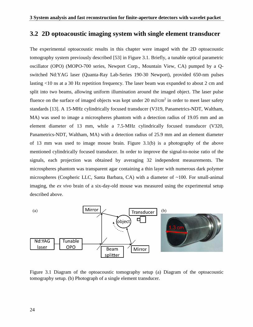
The experimental optoacoustic results in this chapter were imaged with the 2D optoacoustic
tomography system previously described [53] in Figure 3.1. Briefly, a tunable optical parametric
oscillator (OPO) (MOPO-700 series, Newport Corp., Mountain View, CA) pumped by a Q-
switched Nd:YAG laser (Quanta-Ray Lab-Series 190-30 Newport), provided 650-nm pulses
lasting <10 ns at a 30 Hz repetition frequency. The laser beam was expanded to about 2 cm and
split into two beams, allowing uniform illumination around the imaged object. The laser pulse
fluence on the surface of imaged objects was kept under 20 mJ/cm2 in order to meet laser safety
standards [13]. A 15-MHz cylindrically focused transducer (V319, Panametrics-NDT, Waltham,
MA) was used to image a microspheres phantom with a detection radius of 19.05 mm and an
element diameter of 13 mm, while a 7.5-MHz cylindrically focused transducer (V320,
Panametrics-NDT, Waltham, MA) with a detection radius of 25.9 mm and an element diameter
of 13 mm was used to image mouse brain. Figure 3.1(b) is a photography of the above
mentioned cylindrically focused transducer. In order to improve the signal-to-noise ratio of the
signals, each projection was obtained by averaging 32 independent measurements. The
microspheres phantom was transparent agar containing a thin layer with numerous dark polymer
microspheres (Cospheric LLC, Santa Barbara, CA) with a diameter of ~100. For small-animal
imaging, the ex vivo brain of a six-day-old mouse was measured using the experimental setup
described above.
Figure 3.1 Diagram of the optoacoustic tomography setup (a) Diagram of the optoacoustic
tomography setup. (b) Photograph of a single element transducer.
3.3 Problem statement
25
3.3 Problem statement
The model-based reconstruction for a finite-aperture size transducer is described in section 2.2.5
and involves the following matrix relation:
det det
p = M z (3.1)
where detp is a column vector representing the measured acoustic waves at various detector
positions and times; z is a column vector representing the object values; and detM is the
forward model matrix.
The following discussion assumes a 360º projection circular-detection geometry with a radius of
4 cm and line-segment detectors of various lengths up to 20 mm. The image grid is 150 150 (2
cm 2 cm). A total of 360 projections/measurements are taken at uniform intervals over 360º;
each projection has 489 time points. The size of the model matrix detM is 17604022500. To
store all the elements of the model matrix detM as double class, 39 GB of memory are needed.
However, when only nonzero matrix elements are saved (matrix sparsity), the memory required
to store the matrix falls to 0.7-2.7 GB, depending on the length of the detector (Figure 3.2). Thus,
the high memory requirements make pseudo-inversion unsuitable for calculating †
detM in high-
resolution imaging.
Tikhonov regularization-based inversion (section 2.4.2) may be applied to matrices that are
significantly larger than those on which TSVD may be practically applied, facilitating the
reconstruction of high-resolution images. For example, in limited-view scenarios [30], [38], [54],
the tomographic data may not be sufficient to accurately reconstruct all the features in the images.
In such cases, the model matrix detM is ill-conditioned and its inversion requires regularization,
which can suppress the effects of noise and artifacts in the image, e.g. stripe artifacts that appear
with limited tomographic views [30].
3 System analysis and fast reconstruction for finite-aperture detectors with wavelet packet
26
Figure 3.2 Amount of memory required to store the model matrix described in Sec. 2.2.5 when
sparsity is exploited (only non-zero entries are saved). The longer the detector is, the more
memory is required. Without sparsity, the matrix occupies 39 GB of memory. (taken from [26])
3.4 2D Wavelet packets
All wavelet packets/wavelet in this thesis are presented in the discrete form as conjugate mirror
filter banks [55], so only orthogonal wavelets, such as the Daubechies wavelets, are considered.
The Daubechies wavelets are not defined in terms of the resulting scaling and wavelet functions;
instead they are generated numerically using the cascade algorithm [55]. Both the scaling
sequence [ ]h n (Low-pass filter) and the wavelet sequence [ ]g n (high-pass Filter) will here be
normalized to have sum equal 2 , and both sequences (Assume have a length of 2L ) and all
shifts of them by an even number of coefficients are orthonormal to each other.
[2 1 ]
[ ][2 1 ]
h L n n oddg n
h L n n even
(3.2)
A first level discrete wavelet decomposition of a 2D signal [ , ]U x y ( 1... ; 1...x X y Y ) is shown
in Figure 3.3 and defined as
,
[ , ] [ , ] [ 2 ] [ 2 ] [ , ]i j
a x y U i j h i x h j y U i j
A (3.3)
3.4 2D wavelet packets
27
1
,
[ , ] [ , ] [ 2 ] [ 2 ] [ , ]i j
d x y U i j h i x g j y U i j
1D (3.4)
2 2
,
[ , ] [ , ] g[ 2 ]h[ 2 ] [ , ]i j
d x y U i j i x j y U i j
D (3.5)
3 3
,
[ , ] [ , ] g[ 2 ] [ 2 ] [ , ]i j
d x y U i j i x g j y U i j
D (3.6)
Figure 3.3 First level of 2D wavelet packet decomposition with scaling sequence and wavelet
sequence.
The wavelet reconstruction formula is given as
,
1
,
2
,
3
,
[ , ] [ 2 ] [ 2 ] [ , ]
[ 2 ] [ 2 ] [ , ]
[ 2 ] [ 2 ] [ , ]
[ 2 ] [ 2 ] [ , ]
i j
i j
i j
i j
U x y h x i h y j a i j
h x i g y j d i j
g x i h y j d i j
g x i g y j d i j
(3.7)
3 System analysis and fast reconstruction for finite-aperture detectors with wavelet packet
28
A represents the low-passing operation to get the approximation coefficients [ , ]a x y , whereas
1D , 2D and 3D represent high-passing operation to get the three detail coefficients 1[ , ]d x y ,
2[ , ]d x y ,and 3[ , ]d x y over horizontal, vertical and diagonal axes [55]. Only the approximation
coefficients are further decomposed in wavelet decomposition, whereas both approximation and
detail coefficients will be further decomposed wavelet-packet decomposition. A full-tree
decomposition of level/depth I is defined as decomposition where all coefficients were
decomposed I time. A schematic description of a decomposition of level 2 is shown in Figure
3.4. Each leaf corresponds to a distinct spectral band, where all the spectral bands have
approximately the same bandwidth.
Figure 3.4 Full-tree 2D wavelet packet decomposition of level 2.
3.5 Methods
The proposed reconstruction method, GWP-IMMI-FAD, is described as follows. First, we define
wz as the WP-coefficient vector of the object, where the reconstruction of z from wz is given
by
wz = Rz (3.8)
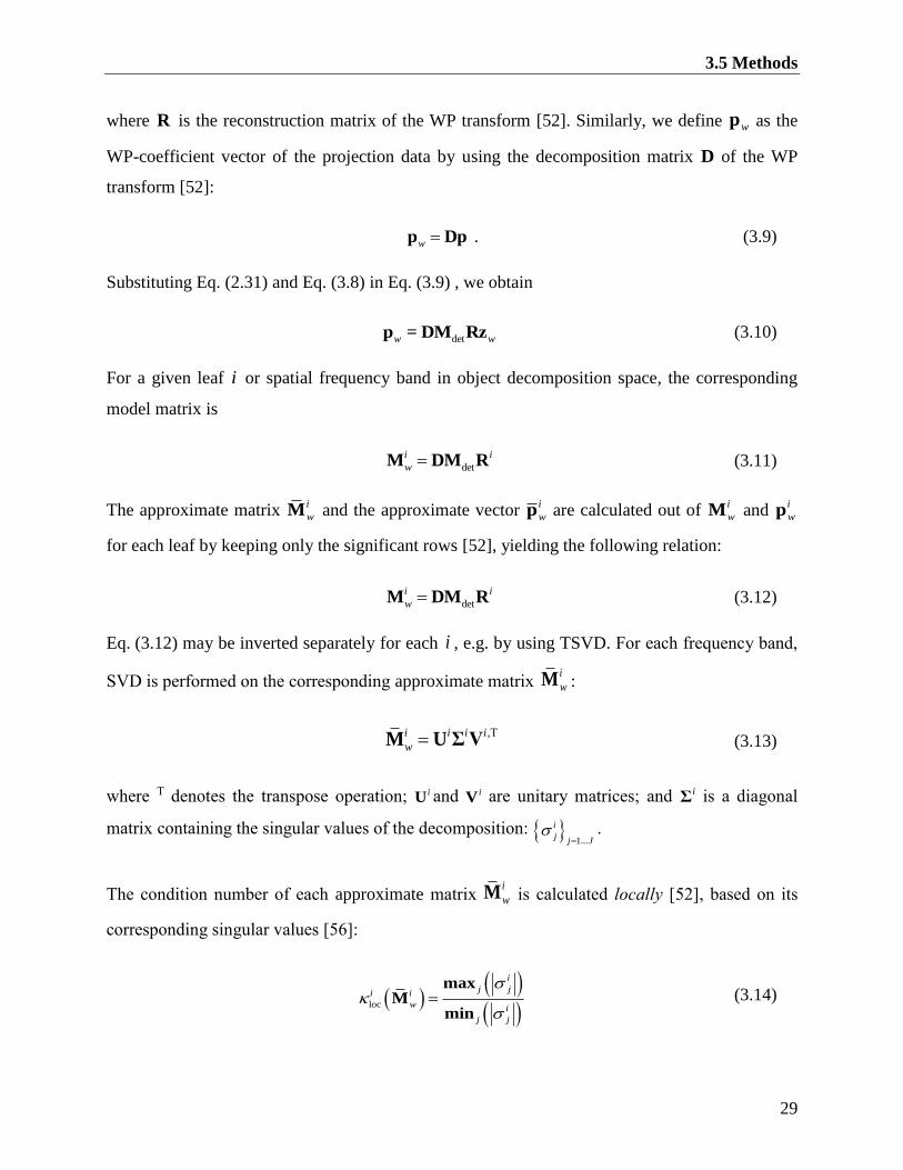
3.5 Methods
29
where R is the reconstruction matrix of the WP transform [52]. Similarly, we define wp as the
WP-coefficient vector of the projection data by using the decomposition matrix D of the WP
transform [52]:
w p Dp . (3.9)
Substituting Eq. (2.31) and Eq. (3.8) in Eq. (3.9) , we obtain
detw wp = DM Rz (3.10)
For a given leaf i or spatial frequency band in object decomposition space, the corresponding
model matrix is
det
i i
w M DM R (3.11)
The approximate matrix i
wM and the approximate vector i
wp are calculated out of i
wM and i
wp
for each leaf by keeping only the significant rows [52], yielding the following relation:
det
i i
w M DM R (3.12)
Eq. (3.12) may be inverted separately for each i , e.g. by using TSVD. For each frequency band,
SVD is performed on the corresponding approximate matrix i
wM :
,T
M U Σ Vi i i i
w (3.13)
where T denotes the transpose operation; iU and i
V are unitary matrices; and Σi is a diagonal
matrix containing the singular values of the decomposition: 1...
i
jj J
.
The condition number of each approximate matrix i
wM is calculated locally [52], based on its
corresponding singular values [56]:
loc
i
j ji i
w i
j j
maxM
min
(3.14)
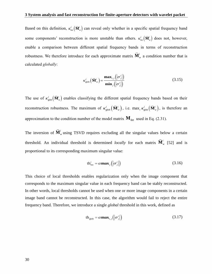
3 System analysis and fast reconstruction for finite-aperture detectors with wavelet packet
30
Based on this definition, loc
i i
w M can reveal only whether in a specific spatial frequency band
some components’ reconstruction is more unstable than others. loc
i i
w M does not, however,
enable a comparison between different spatial frequency bands in terms of reconstruction
robustness. We therefore introduce for each approximate matrix i
wM a condition number that is
calculated globally:
,
glob
i
i j ji i
w i
j j
maxM
min
(3.15)
The use of glob
i i
w M enables classifying the different spatial frequency bands based on their
reconstruction robustness. The maximum of glob
i i
w M , i.e. globmax i i
i w M , is therefore an
approximation to the condition number of the model matrix detM used in Eq. (2.31).
The inversion of i
wM using TSVD requires excluding all the singular values below a certain
threshold. An individual threshold is determined locally for each matrix i
wM [52] and is
proportional to its corresponding maximum singular value:
locth maxi i
j j (3.16)
This choice of local thresholds enables regularization only when the image component that
corresponds to the maximum singular value in each frequency band can be stably reconstructed.
In other words, local thresholds cannot be used when one or more image components in a certain
image band cannot be reconstructed. In this case, the algorithm would fail to reject the entire
frequency band. Therefore, we introduce a single global threshold in this work, defined as
glob ,th maxi
i j j (3.17)
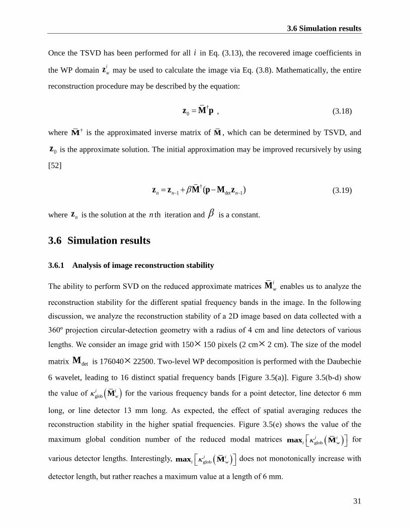
3.6 Simulation results
31
Once the TSVD has been performed for all i in Eq. (3.13), the recovered image coefficients in
the WP domain i
wz may be used to calculate the image via Eq. (3.8). Mathematically, the entire
reconstruction procedure may be described by the equation:
†
0 z M p , (3.18)
where †M is the approximated inverse matrix of M , which can be determined by TSVD, and
0z is the approximate solution. The initial approximation may be improved recursively by using
[52]
†
1 det 1( )n n n z z M p M z (3.19)
where nz is the solution at the thn iteration and is a constant.
3.6 Simulation results
3.6.1 Analysis of image reconstruction stability
The ability to perform SVD on the reduced approximate matrices i
wM enables us to analyze the
reconstruction stability for the different spatial frequency bands in the image. In the following
discussion, we analyze the reconstruction stability of a 2D image based on data collected with a
360º projection circular-detection geometry with a radius of 4 cm and line detectors of various
lengths. We consider an image grid with 150 150 pixels (2 cm 2 cm). The size of the model
matrix detM is 176040 22500. Two-level WP decomposition is performed with the Daubechie
6 wavelet, leading to 16 distinct spatial frequency bands [Figure 3.5(a)]. Figure 3.5(b-d) show
the value of glob
i i
w M for the various frequency bands for a point detector, line detector 6 mm
long, or line detector 13 mm long. As expected, the effect of spatial averaging reduces the
reconstruction stability in the higher spatial frequencies. Figure 3.5(e) shows the value of the
maximum global condition number of the reduced modal matrices globmax Mi i
i w
for
various detector lengths. Interestingly, globmax Mi i
i w
does not monotonically increase with
detector length, but rather reaches a maximum value at a length of 6 mm.
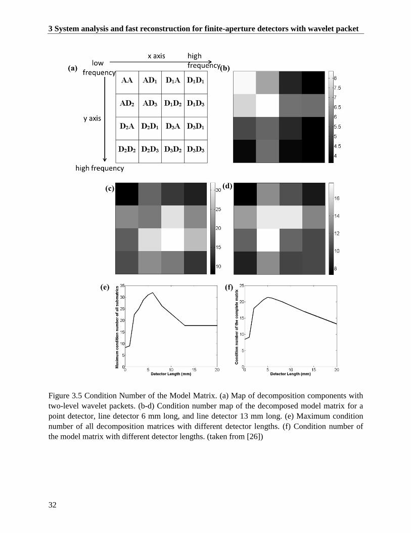
3 System analysis and fast reconstruction for finite-aperture detectors with wavelet packet
32
Figure 3.5 Condition Number of the Model Matrix. (a) Map of decomposition components with
two-level wavelet packets. (b-d) Condition number map of the decomposed model matrix for a
point detector, line detector 6 mm long, and line detector 13 mm long. (e) Maximum condition
number of all decomposition matrices with different detector lengths. (f) Condition number of
the model matrix with different detector lengths. (taken from [26])
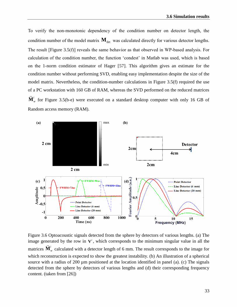
3.6 Simulation results
33
To verify the non-monotonic dependency of the condition number on detector length, the
condition number of the model matrix detM was calculated directly for various detector lengths.
The result [Figure 3.5(f)] reveals the same behavior as that observed in WP-based analysis. For
calculation of the condition number, the function ‘condest’ in Matlab was used, which is based
on the 1-norm condition estimator of Hager [57]. This algorithm gives an estimate for the
condition number without performing SVD, enabling easy implementation despite the size of the
model matrix. Nevertheless, the condition-number calculations in Figure 3.5(f) required the use
of a PC workstation with 160 GB of RAM, whereas the SVD performed on the reduced matrices
i
wM for Figure 3.5(b-e) were executed on a standard desktop computer with only 16 GB of
Random access memory (RAM).
Figure 3.6 Optoacoustic signals detected from the sphere by detectors of various lengths. (a) The
image generated by the row in iV , which corresponds to the minimum singular value in all the
matrices i
wM calculated with a detector length of 6 mm. The result corresponds to the image for
which reconstruction is expected to show the greatest instability. (b) An illustration of a spherical
source with a radius of 200 µm positioned at the location identified in panel (a). (c) The signals
detected from the sphere by detectors of various lengths and (d) their corresponding frequency
content. (taken from [26])
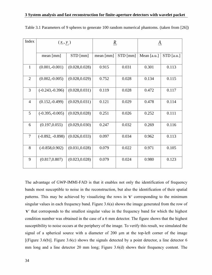
3 System analysis and fast reconstruction for finite-aperture detectors with wavelet packet
34
Table 3.1 Parameters of 9 spheres to generate 100 random numerical phantoms. (taken from [26])
Index ( ,i ix y )
iR iA
mean [mm] STD [mm] mean [mm] STD [mm] Mean [a.u.] STD [a.u.]
1 (0.001,-0.001) (0.028,0.028) 0.915 0.031 0.301 0.113
2 (0.002,-0.005) (0.028,0.029) 0.752 0.028 0.134 0.115
3 (-0.243,-0.396) (0.028,0.031) 0.119 0.028 0.472 0.117
4 (0.152,-0.499) (0.029,0.031) 0.121 0.029 0.478 0.114
5 (-0.395,-0.005) (0.029,0.028) 0.251 0.026 0.252 0.111
6 (0.197,0.055) (0.029,0.030) 0.247 0.032 0.269 0.116
7 (-0.892, -0.898) (0.026,0.033) 0.097 0.034 0.962 0.113
8 (-0.858,0.902) (0.031,0.028) 0.079 0.022 0.971 0.105
9 (0.817,0.807) (0.023,0.028) 0.079 0.024 0.980 0.123
The advantage of GWP-IMMI-FAD is that it enables not only the identification of frequency
bands most susceptible to noise in the reconstruction, but also the identification of their spatial
patterns. This may be achieved by visualizing the rows in iV corresponding to the minimum
singular values in each frequency band. Figure 3.6(a) shows the image generated from the row of
iV that corresponds to the smallest singular value in the frequency band for which the highest
condition number was obtained in the case of a 6 mm detector. The figure shows that the highest
susceptibility to noise occurs at the periphery of the image. To verify this result, we simulated the
signal of a spherical source with a diameter of 200 µm at the top-left corner of the image
[(Figure 3.6(b)]. Figure 3.6(c) shows the signals detected by a point detector, a line detector 6
mm long and a line detector 20 mm long; Figure 3.6(d) shows their frequency content. The
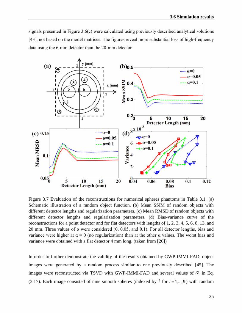
3.6 Simulation results
35
signals presented in Figure 3.6(c) were calculated using previously described analytical solutions
[43], not based on the model matrices. The figures reveal more substantial loss of high-frequency
data using the 6-mm detector than the 20-mm detector.
Figure 3.7 Evaluation of the reconstructions for numerical spheres phantoms in Table 3.1. (a)
Schematic illustration of a random object function. (b) Mean SSIM of random objects with
different detector lengths and regularization parameters. (c) Mean RMSD of random objects with
different detector lengths and regularization parameters. (d) Bias-variance curve of the
reconstructions for a point detector and for flat detectors with lengths of 1, 2, 3, 4, 5, 6, 8, 13, and
20 mm. Three values of α were considered (0, 0.05, and 0.1). For all detector lengths, bias and
variance were higher at α = 0 (no regularization) than at the other α values. The worst bias and
variance were obtained with a flat detector 4 mm long. (taken from [26])
In order to further demonstrate the validity of the results obtained by GWP-IMMI-FAD, object
images were generated by a random process similar to one previously described [45]. The
images were reconstructed via TSVD with GWP-IMMI-FAD and several values of in Eq.
(3.17). Each image consisted of nine smooth spheres (indexed by i for 1,...,9i ) with random
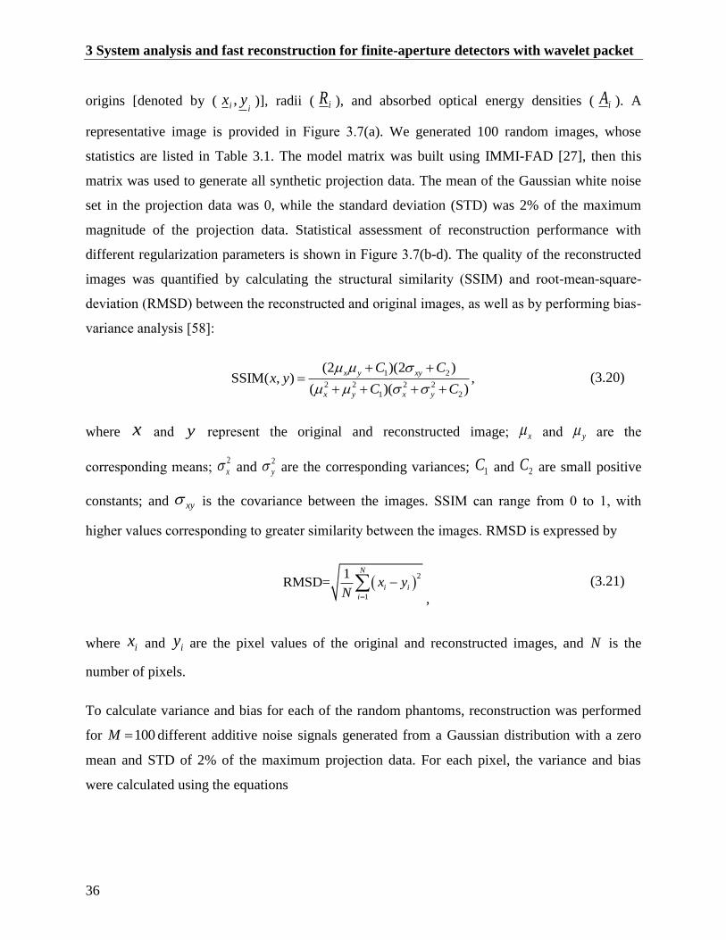
3 System analysis and fast reconstruction for finite-aperture detectors with wavelet packet
36
origins [denoted by ( ,i ix y )], radii ( iR ), and absorbed optical energy densities ( iA ). A
representative image is provided in Figure 3.7(a). We generated 100 random images, whose
statistics are listed in Table 3.1. The model matrix was built using IMMI-FAD [27], then this
matrix was used to generate all synthetic projection data. The mean of the Gaussian white noise
set in the projection data was 0, while the standard deviation (STD) was 2% of the maximum
magnitude of the projection data. Statistical assessment of reconstruction performance with
different regularization parameters is shown in Figure 3.7(b-d). The quality of the reconstructed
images was quantified by calculating the structural similarity (SSIM) and root-mean-square-
deviation (RMSD) between the reconstructed and original images, as well as by performing bias-
variance analysis [58]:
1 2
2 2 2 2
1 2
(2 )(2 )SSIM( , ) ,
( )( )
x y xy
x y x y
C Cx y
C C
(3.20)
where x and y represent the original and reconstructed image; x and y are the
corresponding means; 2
x and 2
y are the corresponding variances; 1C and 2C are small positive
constants; and xy is the covariance between the images. SSIM can range from 0 to 1, with
higher values corresponding to greater similarity between the images. RMSD is expressed by
2
1
1RMSD=
N
i i
i
x yN
,
(3.21)
where ix and iy are the pixel values of the original and reconstructed images, and N is the
number of pixels.
To calculate variance and bias for each of the random phantoms, reconstruction was performed
for 100M different additive noise signals generated from a Gaussian distribution with a zero
mean and STD of 2% of the maximum projection data. For each pixel, the variance and bias
were calculated using the equations
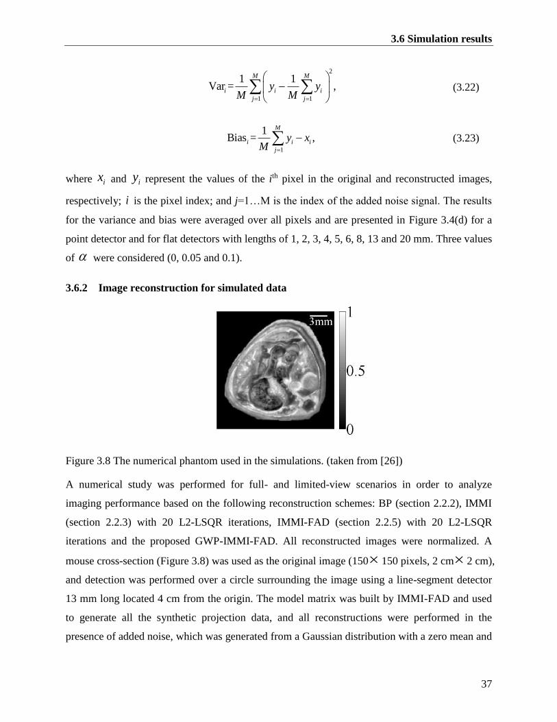
3.6 Simulation results
37
2
1 1
1 1Var = ,
M M
i i i
j j
y yM M
(3.22)
1
1Bias = ,
M
i i i
j
y xM
(3.23)
where ix and iy represent the values of the ith pixel in the original and reconstructed images,
respectively; i is the pixel index; and j=1…M is the index of the added noise signal. The results
for the variance and bias were averaged over all pixels and are presented in Figure 3.4(d) for a
point detector and for flat detectors with lengths of 1, 2, 3, 4, 5, 6, 8, 13 and 20 mm. Three values
of were considered (0, 0.05 and 0.1).
3.6.2 Image reconstruction for simulated data
Figure 3.8 The numerical phantom used in the simulations. (taken from [26])
A numerical study was performed for full- and limited-view scenarios in order to analyze
imaging performance based on the following reconstruction schemes: BP (section 2.2.2), IMMI
(section 2.2.3) with 20 L2-LSQR iterations, IMMI-FAD (section 2.2.5) with 20 L2-LSQR
iterations and the proposed GWP-IMMI-FAD. All reconstructed images were normalized. A
mouse cross-section (Figure 3.8) was used as the original image (150 150 pixels, 2 cm 2 cm),
and detection was performed over a circle surrounding the image using a line-segment detector
13 mm long located 4 cm from the origin. The model matrix was built by IMMI-FAD and used
to generate all the synthetic projection data, and all reconstructions were performed in the
presence of added noise, which was generated from a Gaussian distribution with a zero mean and
3 System analysis and fast reconstruction for finite-aperture detectors with wavelet packet
38
STD of 2% of the maximum projection data. In all cases, the detector was moved in 1°
increments. Reconstructions were performed in Matlab on a personal computer with an Intel
Core i7 2.1 GHz processor and 16 GB of RAM.
In the reconstructions performed with IMMI and IMMI-FAD, the model matrix was invertedd
using Tikhonov regularization. The L-curve method in section 2.4.4 was used to find the
Tikhonov regularization parameter [59]. In the case of GWP-IMMI-FAD, the WP
decomposition was performed using the Daubechies 6 mother wavelet with two-level full-tree
decomposition for both the model matrix and projection data, and inversion was performed using
TSVD. The L-curve method in section 2.4.4 was also used to find the regularization parameter
[59]. Figure 3.9 shows the simulation reconstruction results in a full-view scenario. Figure
3.9(a-d) show the reconstructions using BP, IMMI, IMMI-FAD and GWP-IMMI-FAD. Figure
3.9(e) shows a 1D slice of the reconstructed image taken along the yellow dashed line in Figure
3.9(c). The IMMI reconstruction without accounting for the detector geometry gives a blurry
reconstructed image, as predicted [43], while reconstructions with IMMI-FAD and GWP-IMMI-
FAD are not blurry. The respective SSIMs between the original image and Figure 3.9(a-d) are
0.0753, 0.7023, 0.7748 and 0.7780; the corresponding RMSDs are 0.3860, 0.0961, 0.0357 and
0.0367. The total processingtime needed to build the wavelet-packet decomposition matrices in
advance was approximately 1.2 hours. TSVD was used in GWP-IMMI-FAD, where truncation
was performed by setting 0.02 in Eq. (3.17). Nine iterations of Eq. (3.19) were performed in
GWP-IMMI-FAD, with each iteration lasting 1 s. In this way, after pre-calculation of the
matrices, GWP-IMMI-FAD required only 10 s, whereas Tikhonov regularized IMMI-FAD
required 215 s.
Figure 3.10 shows the images reconstructed from the noisy simulation data for the limited-view
scenario in which only the projections on the left side of the images were used (180-degree
angular coverage). Figure 3.10(a-d) show the reconstructions made using BP, IMMI, IMMI-FAD
and GWP-IMMI-FAD. For comparison, Figure 3.10(e) shows the reconstruction obtained via
WP-IMMI-FAD involving local thresholding [Eq. (3.14)] and the same value as the one used
in Figure 3.10(d). Figure 3.10(f) compares the profiles of absorbed energy density at the same
position in Figure 3.10(c) for the original image and reconstructions made using IMMI-FAD and
GWP-IMMI-FAD. The respective SSIMs between the original image and Figure 3.10(a-e) are
3.7 Experimental results
39
0.0552, 0.4504, 0.6266, 0.6212 and 0.6090; the corresponding RMSDs are 0.4114, 0.1858,
0.0833, 0.0792 and 0.0890. In GWP-IMMI-FAD, TSVD was used in GWP-IMMI-FAD, where
truncation was performed using 0.1 in Eq. (3.17). The total processing time needed to build
the WP decomposition matrices in advance was approximately 40 minutes. Six iterations of Eq.
(3.19) were used for the proposed method, and each iteration required 1 s. As a result, the
reconstruction time of GWP-IMMI-FAD was only 7 s, whereas IMMI-FAD required 104 s.
3.7 Experimental results
We applied GWP-IMMI-FAD to experimental optoacoustic data obtained from a microspheres
phantom and a mouse brain. The microspheres reconstruction was set to a size of 2 cm 2 cm
and 200×200 pixels, while the mouse brain reconstruction was set to 1.3 cm 1.3 cm and
130×130 pixels. All reconstructed images were normalized to their maximum, and negative
values in the images were set to zero.
3.7.1 Microsphere phantom experiment
Figure 3.11(a-d) show the full-view microsphere reconstructions obtained with BP, IMMI,
IMMI-FAD and GWP-IMMI-FAD. In GWP-IMMI-FAD, TSVD was used and truncation was
performed using 0.16 in Eq. (3.17). The reconstruction by GWP-IMMI-FAD is considerably
sharper than those by BP and IMMI, and similar to the one by IMMI-FAD. After pre-calculation
of all matrices, the GWP-IMMI-FAD reconstruction (10 iterations) took only 80 s, whereas the
IMMI-FAD reconstruction required 1646 s.
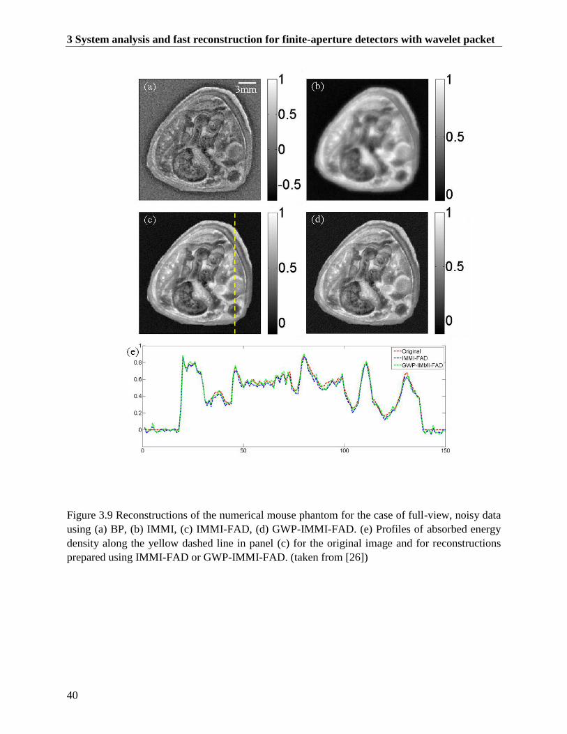
3 System analysis and fast reconstruction for finite-aperture detectors with wavelet packet
40
Figure 3.9 Reconstructions of the numerical mouse phantom for the case of full-view, noisy data
using (a) BP, (b) IMMI, (c) IMMI-FAD, (d) GWP-IMMI-FAD. (e) Profiles of absorbed energy
density along the yellow dashed line in panel (c) for the original image and for reconstructions
prepared using IMMI-FAD or GWP-IMMI-FAD. (taken from [26])
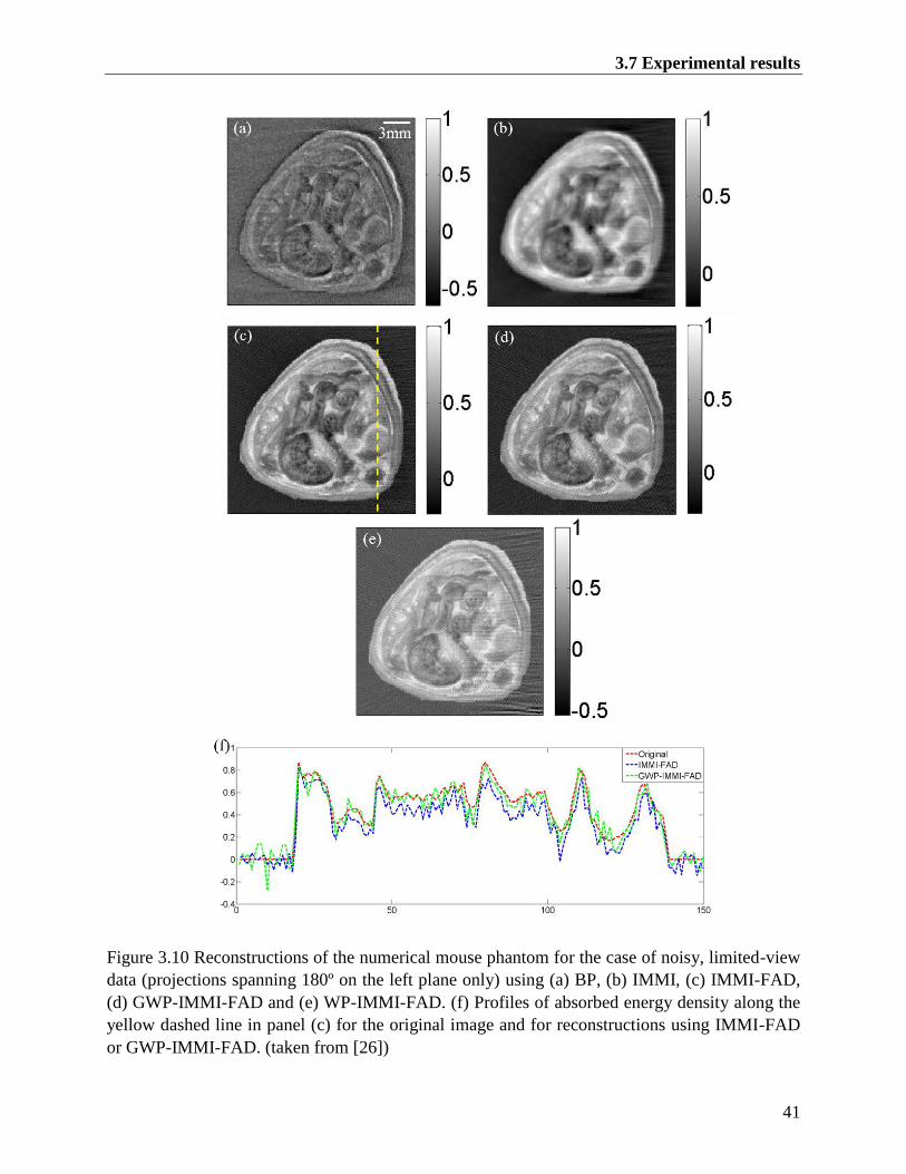
3.7 Experimental results
41
Figure 3.10 Reconstructions of the numerical mouse phantom for the case of noisy, limited-view
data (projections spanning 180º on the left plane only) using (a) BP, (b) IMMI, (c) IMMI-FAD,
(d) GWP-IMMI-FAD and (e) WP-IMMI-FAD. (f) Profiles of absorbed energy density along the
yellow dashed line in panel (c) for the original image and for reconstructions using IMMI-FAD
or GWP-IMMI-FAD. (taken from [26])
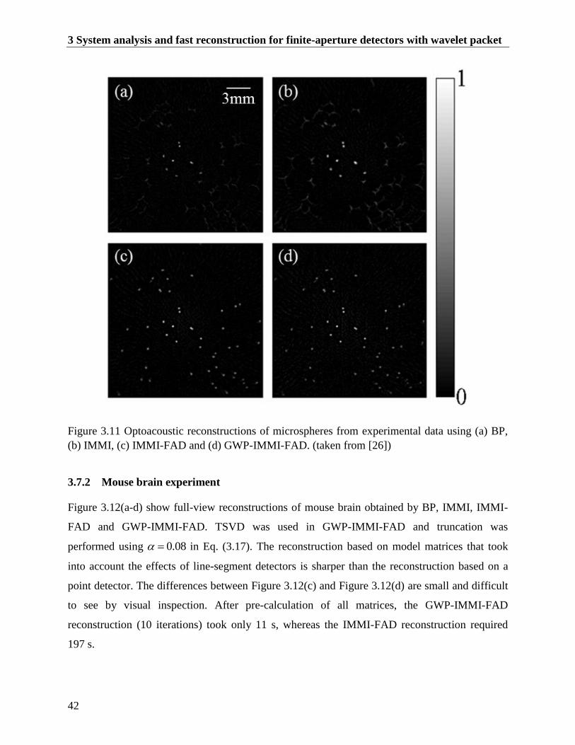
3 System analysis and fast reconstruction for finite-aperture detectors with wavelet packet
42
Figure 3.11 Optoacoustic reconstructions of microspheres from experimental data using (a) BP,
(b) IMMI, (c) IMMI-FAD and (d) GWP-IMMI-FAD. (taken from [26])
3.7.2 Mouse brain experiment
Figure 3.12(a-d) show full-view reconstructions of mouse brain obtained by BP, IMMI, IMMI-
FAD and GWP-IMMI-FAD. TSVD was used in GWP-IMMI-FAD and truncation was
performed using 0.08 in Eq. (3.17). The reconstruction based on model matrices that took
into account the effects of line-segment detectors is sharper than the reconstruction based on a
point detector. The differences between Figure 3.12(c) and Figure 3.12(d) are small and difficult
to see by visual inspection. After pre-calculation of all matrices, the GWP-IMMI-FAD
reconstruction (10 iterations) took only 11 s, whereas the IMMI-FAD reconstruction required
197 s.
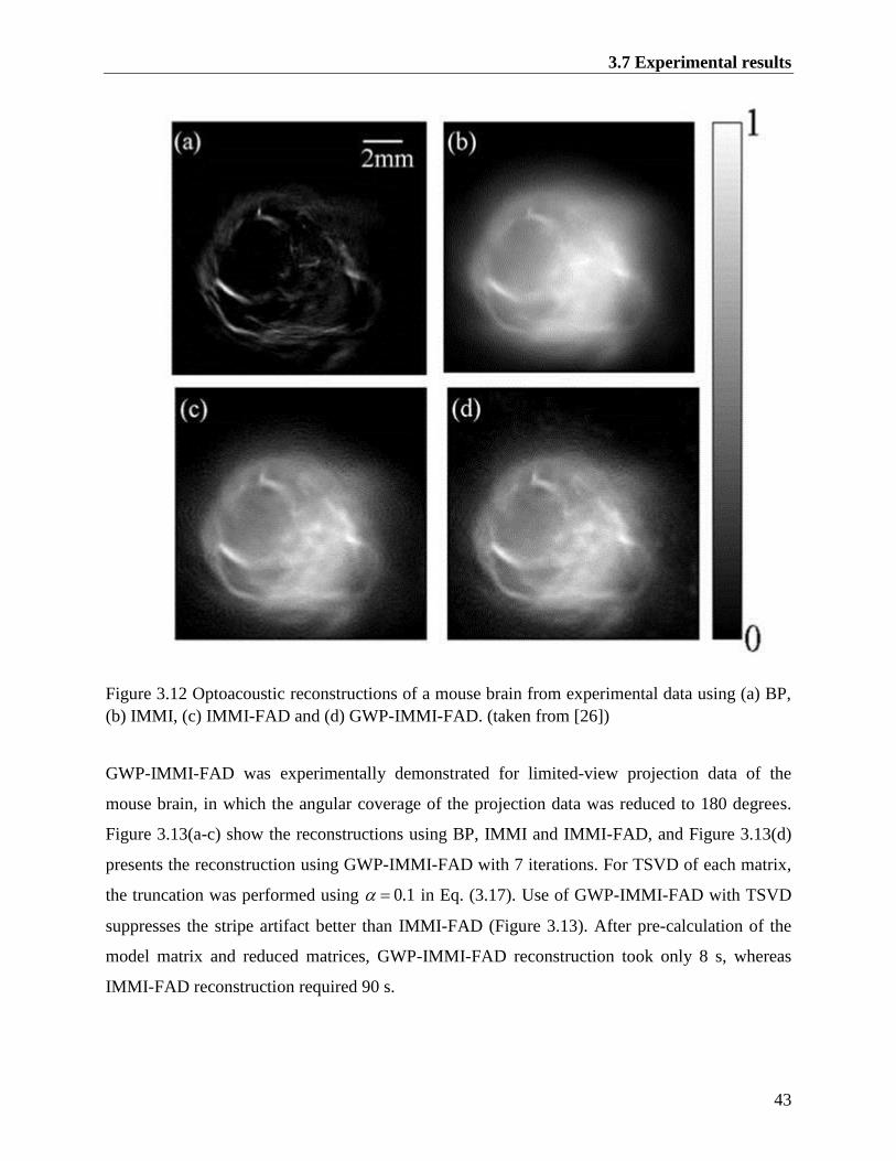
3.7 Experimental results
43
Figure 3.12 Optoacoustic reconstructions of a mouse brain from experimental data using (a) BP,
(b) IMMI, (c) IMMI-FAD and (d) GWP-IMMI-FAD. (taken from [26])
GWP-IMMI-FAD was experimentally demonstrated for limited-view projection data of the
mouse brain, in which the angular coverage of the projection data was reduced to 180 degrees.
Figure 3.13(a-c) show the reconstructions using BP, IMMI and IMMI-FAD, and Figure 3.13(d)
presents the reconstruction using GWP-IMMI-FAD with 7 iterations. For TSVD of each matrix,
the truncation was performed using 0.1 in Eq. (3.17). Use of GWP-IMMI-FAD with TSVD
suppresses the stripe artifact better than IMMI-FAD (Figure 3.13). After pre-calculation of the
model matrix and reduced matrices, GWP-IMMI-FAD reconstruction took only 8 s, whereas
IMMI-FAD reconstruction required 90 s.
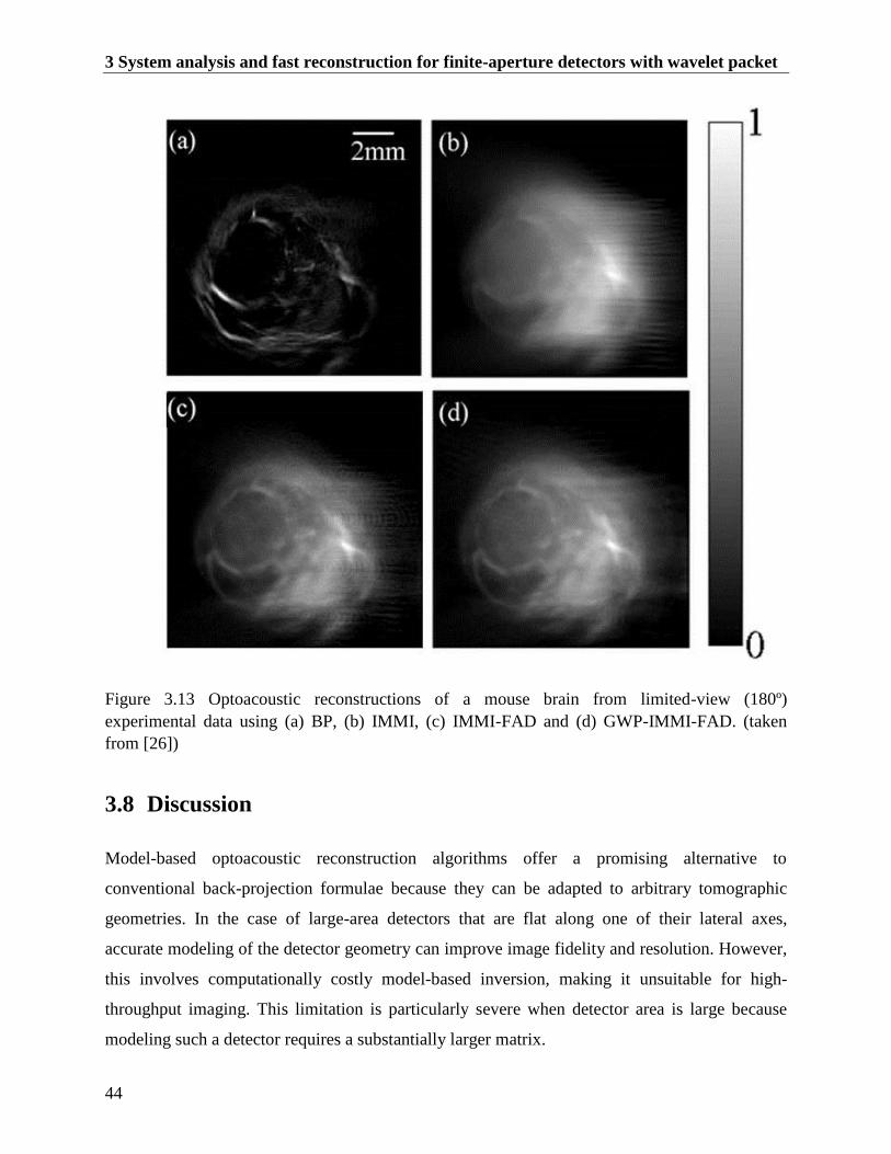
3 System analysis and fast reconstruction for finite-aperture detectors with wavelet packet
44
Figure 3.13 Optoacoustic reconstructions of a mouse brain from limited-view (180º)
experimental data using (a) BP, (b) IMMI, (c) IMMI-FAD and (d) GWP-IMMI-FAD. (taken
from [26])
3.8 Discussion
Model-based optoacoustic reconstruction algorithms offer a promising alternative to
conventional back-projection formulae because they can be adapted to arbitrary tomographic
geometries. In the case of large-area detectors that are flat along one of their lateral axes,
accurate modeling of the detector geometry can improve image fidelity and resolution. However,
this involves computationally costly model-based inversion, making it unsuitable for high-
throughput imaging. This limitation is particularly severe when detector area is large because
modeling such a detector requires a substantially larger matrix.
3.8 Discussion
45
In this chapter we develop GWP-IMMI-FAD, which is the generalization of the WP framework
to finite-aperture detectors. Under the WP framework, the image is divided into a set of spatial
frequency bands that are individually reconstructed from only a fraction of the projection data,
leading to a set of reduced model-matrices. This approach enables the use of TSVD to obtain a
regularized inverse matrix to the tomographic problem. The original matrix, in the case of high-
resolution images, is too large to be inverted using TSVD. Therefore, regularization requires
iterative optimization algorithms, which significantly prolong processing time. One notable
improvement in GWP-IMMI-FAD over the original WP framework is the introduction of a
global threshold for TSVD, which allows GWP-IMMI-FAD to be applied to cases in which
entire spatial frequency bands in the imaged object are difficult to reconstruct, such as in Figure
3.10(d-e).
We show that GWP-IMMI-FAD may be used not only for image reconstruction but also for
system analysis. GWP-IMMI-FAD enables one to calculate the global condition number of each
spatial frequency band, and thus determine the stability of its reconstruction. The use of WPs and
SVD enables one to identify which spatial patterns are most difficult to reconstruct and to
categorize them based on their spatial frequency. We used GWP-IMMI-FAD to analyze the
dependence of reconstruction stability on detector length; we found a non-monotonic
relationship in which the global condition number achieves its maximum with a detector 6 mm
long. This relationship matches well with the variation in condition number of model matrix det
M
with detector length. We show that with SVD, reconstruction instability with a 6-mm detector is
most severe at the periphery of the image (Figure 3.5). We also found that when a small
spherical source is positioned at the corner of the image, the signal detected by a 6-mm detector
is more low-passed than the one detected by a 20-mm detector.
Our results with GWP-IMMI-FAD show inconsistencies with previous work [60] in which the
amount of smearing created by flat detectors was reported to be proportional to the aperture
dimensions. The analysis in that work [60] suggests that longer detectors attenuate high
frequencies in the projection data more strongly than shorter detectors, and that therefore the
global condition number should scale with detector length. However, our analysis shows that a 6-
mm detector attenuates high frequencies more strongly than a 20-mm detector [Figure 3.6(d)].
This apparent contradiction may be resolved by considering that the analysis in the previous

3 System analysis and fast reconstruction for finite-aperture detectors with wavelet packet
46
work [60] was performed for the filtered BP reconstruction algorithm, which assumes an ideal
point detector. In this case, any discrepancy between the forward and inverse models leads to
image distortion and possibly smearing. Indeed, although the signal generated by a 20-mm
detector is sharper than the one generated by a 6-mm detector, it involves a significantly larger
delay when compared to the signal detected by the point detector, as can be seen in Figure 3.6(c).
Reconstruction formulae derived for the case of infinitely long line detectors [61] are also
inconsistent with the previous work based on point detectors [60].
To further validate our conclusions, we compared the reconstructions of randomly generated
images obtained with several detector lengths. The reconstruction results revealed a similar
behavior to those obtained by the SVD analysis of GWP-IMMI-FAD. The highest reconstruction
error was obtained for a 4-mm detector. This differs from the results obtained from SVD analysis,
reflecting the fact that SVD considers all possible images, whereas the randomly generated
images represent only a small portion of all possible images. The similar trends obtained in
Figure 3.5(e-f) and Figure 3.7(b-c) suggest that the analysis described here is valid. Further
validation comes from the bias-variance curves in Figure 3.7(d), which show that the variance
associated with stability and noise amplification exhibits similar non-monotonic behavior as the
condition number prediction in Figure 3.5(e-f) and the results in Figure 3.7(b-c). The condition
numbers and reconstruction errors depend on the resolution specified by the grid on which the
image is represented: increasing the grid resolution should strengthen the effect of detector
length on the condition number of the matrices describing the system.
We showcased the potential of GWP-IMMI-FAD for image reconstruction using simulated and
experimental optoacoustic data under conditions of full- and limited-view tomography. In all
examples, the model matrix was too large for TSVD, so Tikhonov regularization was used
instead. In contrast, the reduced matrices in the wavelet packet decomposition were small
enough to perform TSVD. In the case of full-view simulated and experimental data, GWP-
IMMI-FAD reconstruction quality was similar to the quality of Tikhonov regularization IMMI-
FAD reconstruction. In the case of limited-view simulated data, GWP-IMMI-FAD performed
slightly worse than Tikhonov regularization IMMI-FAD. However, in the case of limited-view
experimental data, GWP-IMMI-FAD reconstruction suppressed stripe artifacts better. In all the
3.8 Discussion
47
examples studied, GWP-IMMI-FAD completed the reconstruction more than 10-fold faster than
IMMI-FAD.
The performance demonstrated in this chapter may prove useful for high-throughput
optoacoustic imaging studies, which can require the reconstruction of thousands of cross-
sectional images. Moreover, the results suggest that the WP framework is not restricted to ideal
imaging scenarios, but that it can be generalized to manage the effects of finite-size aperture and
limited-view tomography. Further generalization may be achieved by applying this framework to
geometries employing focused detectors as well as to 3D reconstruction problems, where the
need for faster model-based reconstructions is even greater. GWP-IMMI-FAD may be useful for
designing optoacoustic systems; for example, it has already demonstrated, for the first time, that
beyond a certain length of finite-aperture detector, further increases in length may lead not only
to stronger optoacoustic signals, but also to stabler reconstructions.

3 System analysis and fast reconstruction for finite-aperture detectors with wavelet packet
48
49
4 Sparsity-based acoustic inversion in cross-
sectional multi-scale optoacoustic imaging
With recent advancements in hardware of optoacoustic imaging systems, highly detailed cross-
sectional images may be acquired with a single laser pulse, thus eliminating motion artifacts.
Nonetheless, other sources of artifacts remain due to signal distortion or out-of-plane signals.
The purpose of image reconstruction algorithms is to obtain the most accurate images from noisy,
distorted projection data. In this chapter, we use the model-based approach for acoustic inversion,
combined with a sparsity-based inversion procedure. Specifically, a cost function is used that
includes the L1 norm of the image in sparse representation and a total variation (TV) term. The
optimization problem is solved by a numerically efficient implementation of a non-linear
gradient descent algorithm. TV-L1 model-based inversion is tested in the cross-sectional
geometry for simulated data as well as for in vivo experimental data from an adult mouse. In all
cases, model-based TV-L1 inversion showed better performance over the conventional Tikhonov
regularization, TV and L1 inversion. In the numerical examples, the images reconstructed with
TV-L1 inversion were quantitatively more similar to the original images. In the experimental
examples, TV-L1 inversion yielded sharper images and weaker streak artifacts. The results
herein show that TV-L1 inversion is capable of improving the quality of highly detailed, multi-
scale optoacoustic images obtained in vivo using cross-sectional imaging systems. As a result of
its high fidelity, model-based TV-L1 inversion may be considered the new standard for image
reconstruction in cross-sectional imaging.
Some of the material in this chapter has been presented in the following publication in a very
similar or identical form to the text in this chapter:
4 Sparsity-based acoustic inversion in cross-sectional multi-scale optoacoustic imaging
50
“Sparsity-based acoustic inversion in cross-sectional multi-scale optoacoustic imaging” by
Yiyong Han, Stratis Tzoumas, Antonio Nunes, Vasilis Ntziachristos, Amir Rosenthal, Medical
Physics, 42(9), 5444-5452, 2015.
4.1 Introduction
In OAT, excitation usually involves short, high-power laser pulses that lead to the generation of
outward propagating acoustic waves, measured over a surface that encompasses the imaged
object [10]. Ideally, the detection surface should completely surround the illuminated region. In
practice, this requirement necessitates scanning an ultrasound array around the specimen, leading
to long imaging durations [29], [62]. An alternative approach is the use of circular detection
arrays cylindrically focused to the plane of interest. By simultaneously reading out all the
detection channels, a 2D cross-sectional optoacoustic image may be formed from a single laser
pulse. This characteristic enables video-rate imaging free of motion artifacts. Recent
improvements in cross-sectional OAT hardware now enables the capture of highly detailed 2D
images, which exhibit features at several scales.
Optoacoustic images are formed from the detected acoustic waves or projection data by using
tomographic reconstruction algorithms [10]. Such algorithms are usually based on either closed-
form solutions in the time or frequency domain or on a model-based approach in which the
relation between the optoacoustic image and measured data is discretized in the form of a matrix
relation. Model-based image reconstruction is performed by inverting the matrix relation. The
advantage of the model-based approach is that it can incorporate arbitrary detection geometries
for which no exact closed-form solution exists. In particular, model-based image reconstruction
has been demonstrated for reducing image distortion and artifacts due to finite detector aperture
or incomplete projection data.
Quite often, regularization is required in model-based inversion to suppress noise and artifacts in
the reconstructed images by making assumptions on the nature of the expected optoacoustic
image. Usually the regularization approaches used, e.g. Tikhonov regularization, penalize the
energy of the reconstructed image. These approaches suppress noise and artifacts, but sometimes
at the cost of image blurring. More recent regularization approaches are based on either
4.2 2D optoacoustic imaging system with curved focused array
51
penalizing the TV term in the image or enforcing sparsity via an alternative representation, e.g. a
wavelet basis. Both regularization approaches have been shown to produce sharper, cleaner
images than energy-minimization regularization in several imaging scenarios, and their
combination has been used in image denoising. Nonetheless, demonstration on experimental data
has been limited to tissue-mimicking phantoms or experiments in mice that focused on imaging
vascularization. In both cases, the structures visualized were relatively simple and were mostly
dominated by a few small-scale features, which are inherently favored by sparsity and TV
constraints. In many applications, cross-sectional optoacoustic images exhibit a rich structure
that cannot be reconstructed so well under such constraints.
In this chapter, we study the performance of the combination of TV- and sparsity-based
regularization strategies in cross-sectional multi-scale optoacoustic imaging. Image
reconstruction is performed for both highly detailed numerical phantoms and cross-sectional
images of an adult mouse obtained in vivo. In both cases, the reconstruction algorithm is tested in
the full- and limited-view scenarios and compared to model-based reconstructions obtained using
Tikhonov regularization, TV and L1 inversion.
The rest of the chapter is organized as follows. In section 4.2, we introduce the cross-sectional
optoacoustic imaging system used in this chapter. Section 4.3 reviews the model-based
reconstruction framework with the various regularization methods. Section 4.4 discusses the
regularization strategies used in our work and the details of the experimental and simulation
studies. The results of simulations and experiments are presented in section 4.5 and section 4.6,
and are evaluated in section 4.7. Finally the discussion and conclusions are given in section 4.8.
4.2 2D optoacoustic imaging system with curved focused array
The 2D sparsity-based reconstruction in this chapter is proposed for the cross-sectional system
previously described [63] (Figure 4.1). Briefly, a tunable OPO pumped by a ND:YAG laser
(Opotek Inc., Carlsbad, CA) was employed with energy of up to 20 mJ/cm2, wavelengths from
680 nm to 980 nm, pulse duration of 8 ns, and a pulse repetition rate of 10 Hz. All data were
acquired after excitation at the single wavelength of 900 nm. A 10-arm fiber bundle was used to
provide uniform light-sheet illumination in the imaged plane with a width of 8 mm. A custom-
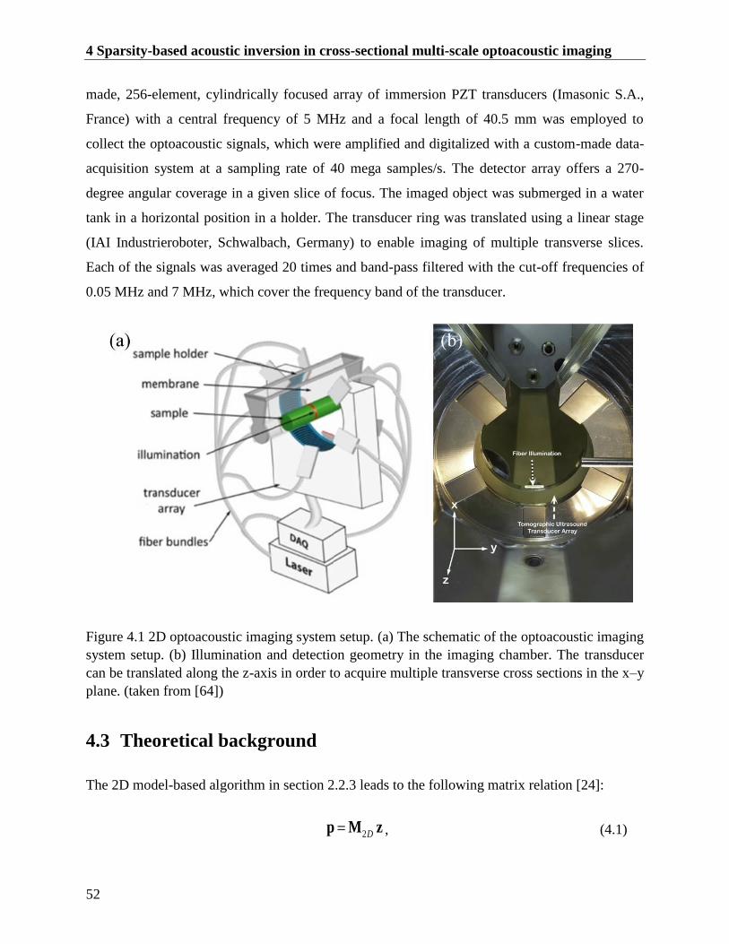
4 Sparsity-based acoustic inversion in cross-sectional multi-scale optoacoustic imaging
52
made, 256-element, cylindrically focused array of immersion PZT transducers (Imasonic S.A.,
France) with a central frequency of 5 MHz and a focal length of 40.5 mm was employed to
collect the optoacoustic signals, which were amplified and digitalized with a custom-made data-
acquisition system at a sampling rate of 40 mega samples/s. The detector array offers a 270-
degree angular coverage in a given slice of focus. The imaged object was submerged in a water
tank in a horizontal position in a holder. The transducer ring was translated using a linear stage
(IAI Industrieroboter, Schwalbach, Germany) to enable imaging of multiple transverse slices.
Each of the signals was averaged 20 times and band-pass filtered with the cut-off frequencies of
0.05 MHz and 7 MHz, which cover the frequency band of the transducer.
Figure 4.1 2D optoacoustic imaging system setup. (a) The schematic of the optoacoustic imaging
system setup. (b) Illumination and detection geometry in the imaging chamber. The transducer
can be translated along the z-axis in order to acquire multiple transverse cross sections in the x–y
plane. (taken from [64])
4.3 Theoretical background
The 2D model-based algorithm in section 2.2.3 leads to the following matrix relation [24]:
2Dp M z , (4.1)
4.3 Theoretical background
53
where p is a column vector representing the measurement data, z is a column vector
representing the unknown reconstruction image and 2DM is the forward model matrix. For a
given optoacoustic imaging system, the model matrix 2DM depends solely on the image grid
and the measurement geometry.
4.3.1 Tikhonov regularization with Laplacian operation
When regularization is required, e.g. in the case of insufficient projection data, Tikhonov
regularization in section 2.4.2 is often used [59]:
2 2
2 2 2argmin
D
z
p M z Lz , (4.2)
where 0 is the regularization parameter and L is the regularization operator. In this chapter,
a quadratic smoothness Laplacian penalty term is used [38]:
2 2
1 1 1 121
4N
n n n n n
x y x y x y x y x y
n
( , ) ( , ) ( , ) ( , ) ( , )Lz ( z z z z z ) . (4.3)
where N is the total pixel number of the image z and n
x y( , )z is the intensity of the thn pixel at
the position of ( , )x y . Tikhonov regularization with a Laplacian penalty (Tik-Lap) may be
efficiently performed using the LSQR algorithm.
4.3.2 L1 regularization
The application of L1 regularization for inverting Eq. (4.1) is based on the common assumption
that the reconstructed image may be sparsely represented in an alternative basis [36], [65]–[68].
To perform the inversion, the following procedure is applied. First, the image to be recovered u
is transferred into a basis in which it is expected to be sparse: x Φz , where x is the
representation of z in the new domain and Φ is the transform matrix. Generally, a unitary Φ
would be preferable, which represents a transformation to an orthonormal basis. In this chapter,
Φ was chosen to represent a three-level Daubechies 4 wavelet transform. L1 regularization can
then be described by solving the following problem:
4 Sparsity-based acoustic inversion in cross-sectional multi-scale optoacoustic imaging
54
2
2 2 1argmin
D
z
p M z Φz , (4.4)
where 0 is the regularization parameter.
We calculate the L1 norm and its derivative as following. The L1 norm is the sum of absolute
values. Let u Φz and we can approximate the absolute value of u as Tu u , where is
a small positive constant. And we can get the derivative 1d
d
T
u u
u u u [69].
4.3.3 TV regularization
TV regularization is used for the suppression of noise [70] as well as streak artifacts [71][38],
[72]–[74]. The scheme has the following expression:
2
2 2 TVargmin
D
z
p M z z , (4.5)
where 0 is the regularization parameter. And the TV norm is defined as
22
TV x y
i j
i j i j ,
z z( , ) z( , ) , (4.6)
where x and
y represent the finite differences of the image along x and y directions.
4.4 Combined TV-L1 sparsity-based reconstruction
Here we demonstrate the use of combined TV-L1 regularization for image reconstruction in
cross-sectional optoacoustic imaging. Image reconstruction is performed by solving the
following problem:
2
2 1 22 TV 1argmin argmin
D
z z
(z) p M z z Φzf . (4.7)
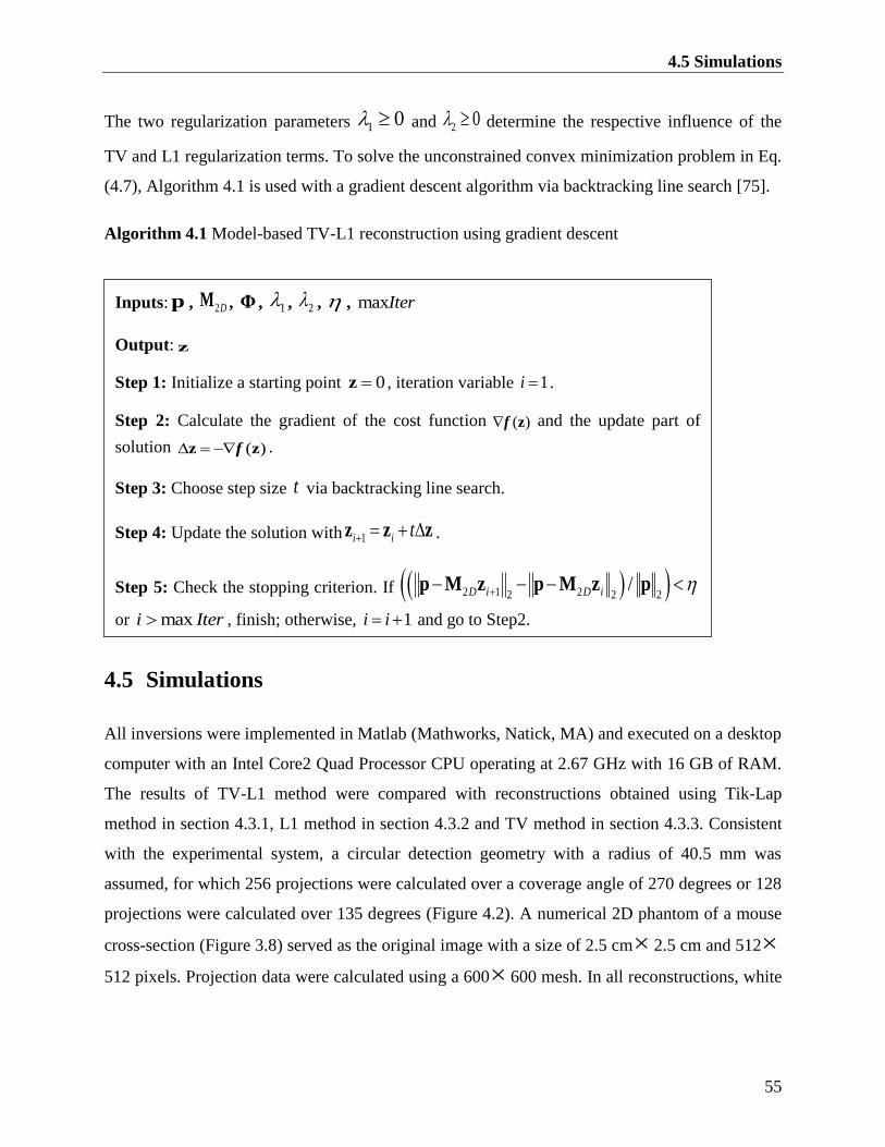
4.5 Simulations
55
The two regularization parameters 10 and 2
0 determine the respective influence of the
TV and L1 regularization terms. To solve the unconstrained convex minimization problem in Eq.
(4.7), Algorithm 4.1 is used with a gradient descent algorithm via backtracking line search [75].
Algorithm 4.1 Model-based TV-L1 reconstruction using gradient descent
4.5 Simulations
All inversions were implemented in Matlab (Mathworks, Natick, MA) and executed on a desktop
computer with an Intel Core2 Quad Processor CPU operating at 2.67 GHz with 16 GB of RAM.
The results of TV-L1 method were compared with reconstructions obtained using Tik-Lap
method in section 4.3.1, L1 method in section 4.3.2 and TV method in section 4.3.3. Consistent
with the experimental system, a circular detection geometry with a radius of 40.5 mm was
assumed, for which 256 projections were calculated over a coverage angle of 270 degrees or 128
projections were calculated over 135 degrees (Figure 4.2). A numerical 2D phantom of a mouse
cross-section (Figure 3.8) served as the original image with a size of 2.5 cm 2.5 cm and 512
512 pixels. Projection data were calculated using a 600 600 mesh. In all reconstructions, white
Inputs: p , 2DM , Φ , 1
, 2 , , maxIter
Output: z
Step 1: Initialize a starting point 0z , iteration variable 1i .
Step 2: Calculate the gradient of the cost function ( ) zf and the update part of
solution ( ) z zf .
Step 3: Choose step size t via backtracking line search.
Step 4: Update the solution with 1i i t z z z .
Step 5: Check the stopping criterion. If 2 1 22 2 2/D i D i p M z p M z p
or maxi Iter , finish; otherwise, 1i i and go to Step2.
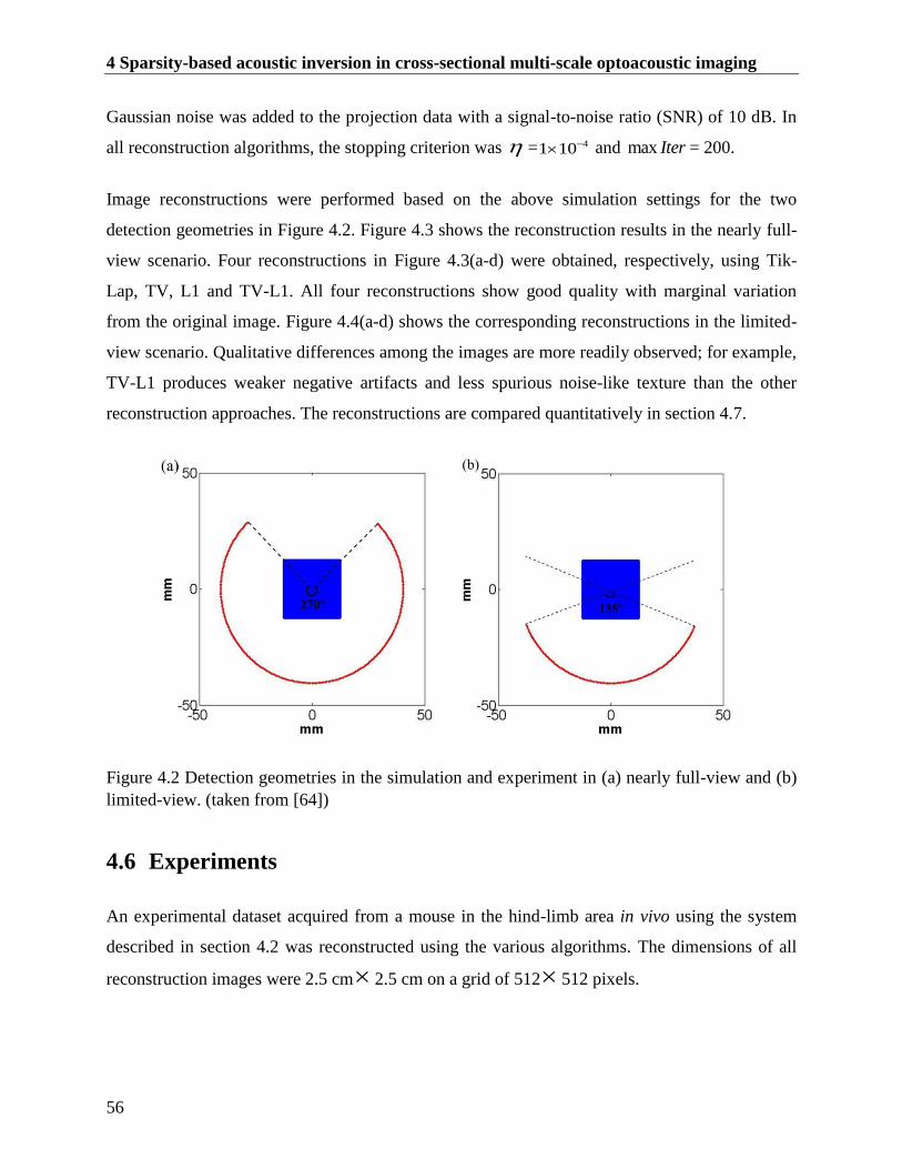
4 Sparsity-based acoustic inversion in cross-sectional multi-scale optoacoustic imaging
56
Gaussian noise was added to the projection data with a signal-to-noise ratio (SNR) of 10 dB. In
all reconstruction algorithms, the stopping criterion was = 41 10 and max Iter = 200.
Image reconstructions were performed based on the above simulation settings for the two
detection geometries in Figure 4.2. Figure 4.3 shows the reconstruction results in the nearly full-
view scenario. Four reconstructions in Figure 4.3(a-d) were obtained, respectively, using Tik-
Lap, TV, L1 and TV-L1. All four reconstructions show good quality with marginal variation
from the original image. Figure 4.4(a-d) shows the corresponding reconstructions in the limited-
view scenario. Qualitative differences among the images are more readily observed; for example,
TV-L1 produces weaker negative artifacts and less spurious noise-like texture than the other
reconstruction approaches. The reconstructions are compared quantitatively in section 4.7.
Figure 4.2 Detection geometries in the simulation and experiment in (a) nearly full-view and (b)
limited-view. (taken from [64])
4.6 Experiments
An experimental dataset acquired from a mouse in the hind-limb area in vivo using the system
described in section 4.2 was reconstructed using the various algorithms. The dimensions of all
reconstruction images were 2.5 cm 2.5 cm on a grid of 512 512 pixels.
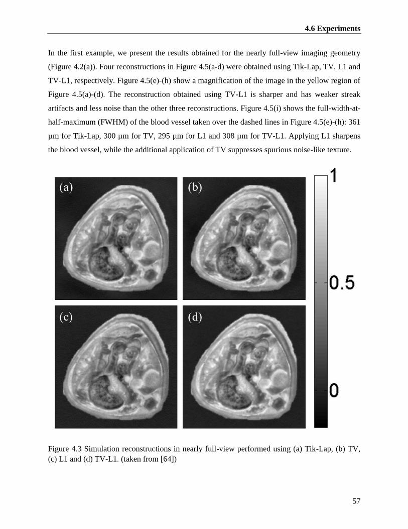
4.6 Experiments
57
In the first example, we present the results obtained for the nearly full-view imaging geometry
(Figure 4.2(a)). Four reconstructions in Figure 4.5(a-d) were obtained using Tik-Lap, TV, L1 and
TV-L1, respectively. Figure 4.5(e)-(h) show a magnification of the image in the yellow region of
Figure 4.5(a)-(d). The reconstruction obtained using TV-L1 is sharper and has weaker streak
artifacts and less noise than the other three reconstructions. Figure 4.5(i) shows the full-width-at-
half-maximum (FWHM) of the blood vessel taken over the dashed lines in Figure 4.5(e)-(h): 361
µm for Tik-Lap, 300 µm for TV, 295 µm for L1 and 308 µm for TV-L1. Applying L1 sharpens
the blood vessel, while the additional application of TV suppresses spurious noise-like texture.
Figure 4.3 Simulation reconstructions in nearly full-view performed using (a) Tik-Lap, (b) TV,
(c) L1 and (d) TV-L1. (taken from [64])
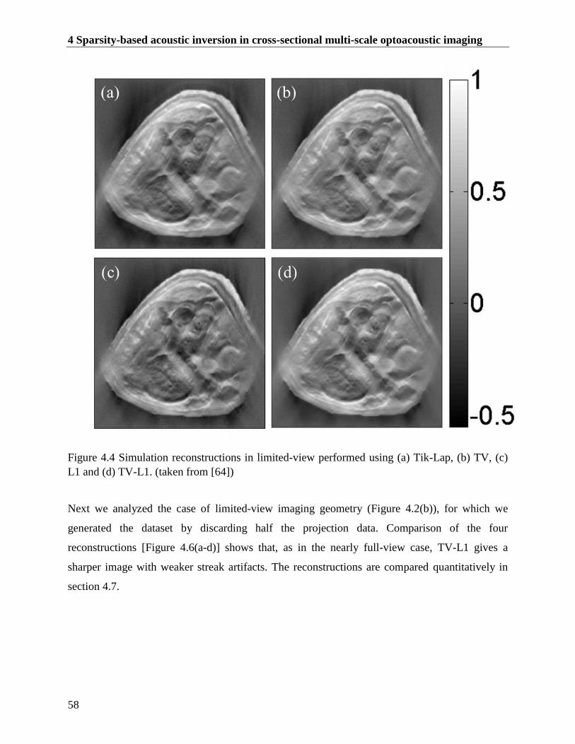
4 Sparsity-based acoustic inversion in cross-sectional multi-scale optoacoustic imaging
58
Figure 4.4 Simulation reconstructions in limited-view performed using (a) Tik-Lap, (b) TV, (c)
L1 and (d) TV-L1. (taken from [64])
Next we analyzed the case of limited-view imaging geometry (Figure 4.2(b)), for which we
generated the dataset by discarding half the projection data. Comparison of the four
reconstructions [Figure 4.6(a-d)] shows that, as in the nearly full-view case, TV-L1 gives a
sharper image with weaker streak artifacts. The reconstructions are compared quantitatively in
section 4.7.
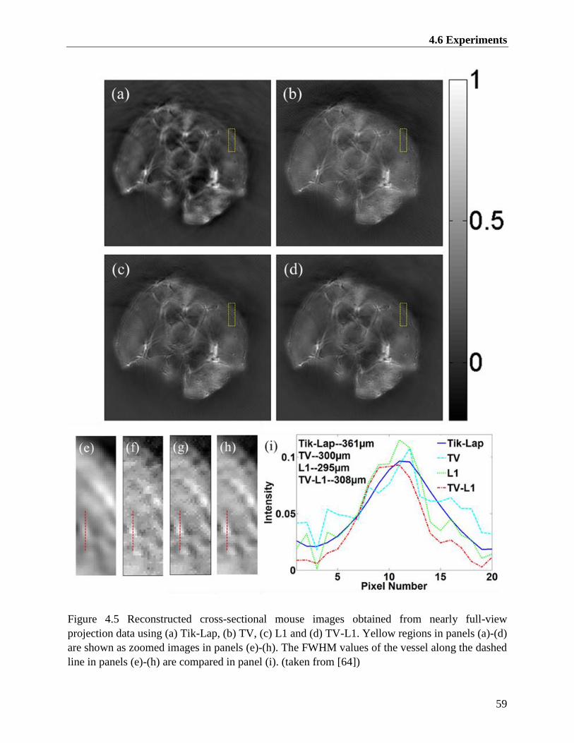
4.6 Experiments
59
Figure 4.5 Reconstructed cross-sectional mouse images obtained from nearly full-view
projection data using (a) Tik-Lap, (b) TV, (c) L1 and (d) TV-L1. Yellow regions in panels (a)-(d)
are shown as zoomed images in panels (e)-(h). The FWHM values of the vessel along the dashed
line in panels (e)-(h) are compared in panel (i). (taken from [64])
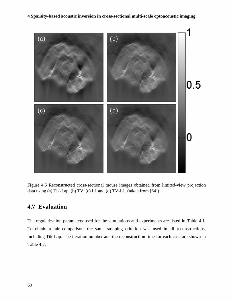
4 Sparsity-based acoustic inversion in cross-sectional multi-scale optoacoustic imaging
60
Figure 4.6 Reconstructed cross-sectional mouse images obtained from limited-view projection
data using (a) Tik-Lap, (b) TV, (c) L1 and (d) TV-L1. (taken from [64])
4.7 Evaluation
The regularization parameters used for the simulations and experiments are listed in Table 4.1.
To obtain a fair comparison, the same stopping criterion was used in all reconstructions,
including Tik-Lap. The iteration number and the reconstruction time for each case are shown in
Table 4.2.
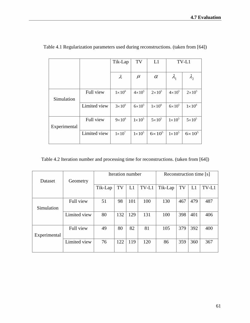
4.7 Evaluation
61
Table 4.1 Regularization parameters used during reconstructions. (taken from [64])
Tik-Lap TV L1 TV-L1
1 2
Simulation
Full view 61 10 54 10 52 10 54 10 52 10
Limited view 63 10 56 10 61 10 56 10 61 10
Experimental
Full view 69 10 51 10 55 10 51 10 55 10
Limited view 71 10 51 10 56 10 51 10 56 10
Table 4.2 Iteration number and processing time for reconstructions. (taken from [64])
Dataset Geometry
Iteration number Reconstruction time [s]
Tik-Lap TV L1 TV-L1 Tik-Lap TV L1 TV-L1
Simulation
Full view 51 98 101 100 130 467 479 487
Limited view 80 132 129 131 100 398 401 406
Experimental
Full view 49 80 82 81 105 379 392 400
Limited view 76 122 119 120 86 359 360 367
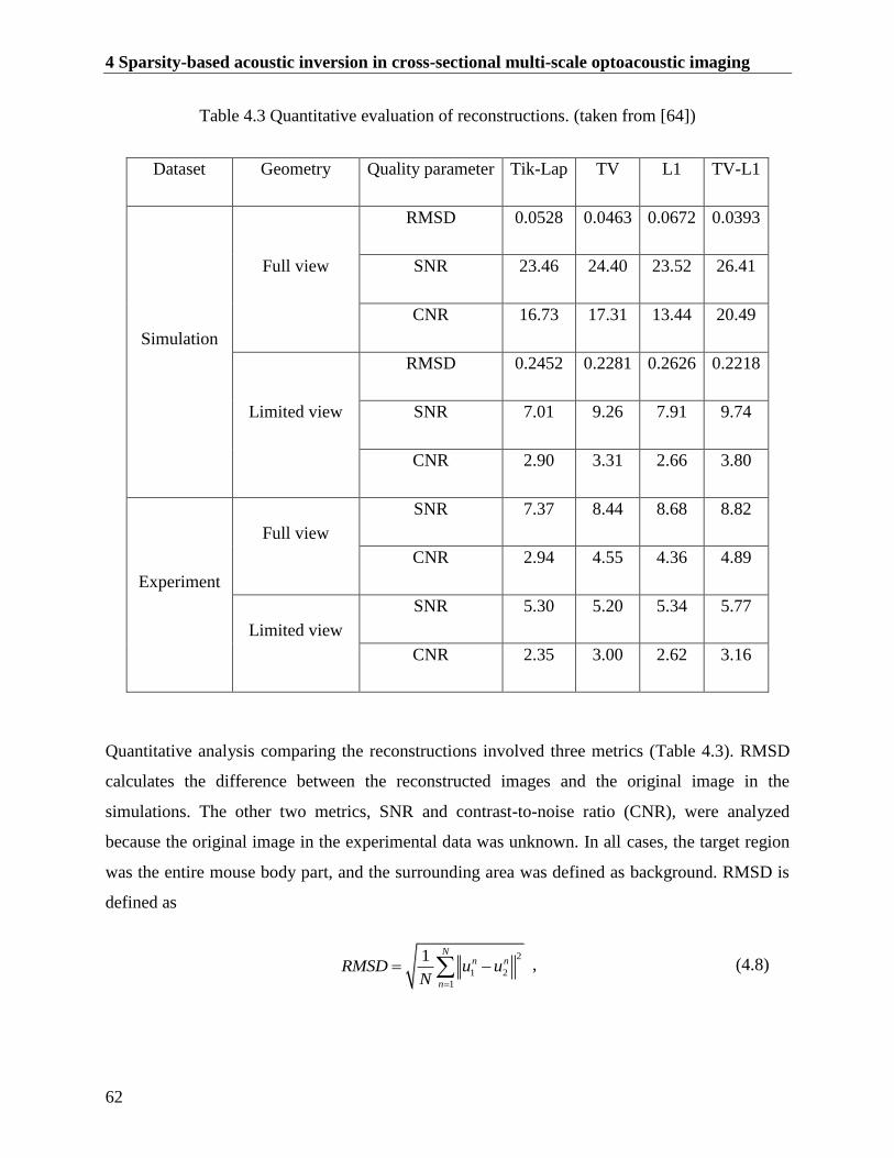
4 Sparsity-based acoustic inversion in cross-sectional multi-scale optoacoustic imaging
62
Table 4.3 Quantitative evaluation of reconstructions. (taken from [64])
Dataset Geometry Quality parameter Tik-Lap TV L1 TV-L1
Simulation
Full view
RMSD 0.0528 0.0463 0.0672 0.0393
SNR 23.46 24.40 23.52 26.41
CNR 16.73 17.31 13.44 20.49
Limited view
RMSD 0.2452 0.2281 0.2626 0.2218
SNR 7.01 9.26 7.91 9.74
CNR 2.90 3.31 2.66 3.80
Experiment
Full view
SNR 7.37 8.44 8.68 8.82
CNR 2.94 4.55 4.36 4.89
Limited view
SNR 5.30 5.20 5.34 5.77
CNR 2.35 3.00 2.62 3.16
Quantitative analysis comparing the reconstructions involved three metrics (Table 4.3). RMSD
calculates the difference between the reconstructed images and the original image in the
simulations. The other two metrics, SNR and contrast-to-noise ratio (CNR), were analyzed
because the original image in the experimental data was unknown. In all cases, the target region
was the entire mouse body part, and the surrounding area was defined as background. RMSD is
defined as
2
1 2
1
1 Nn n
n
RMSD u uN
, (4.8)
4.8 Discussion and conclusion
63
where 1
nu and 2
nu are the thn pixel value of the two images 1u and 2
u , and N is the total pixel
number of the image. SNR is defined as
10
20( )
( )log
t
dB b
ASNR
A
, (4.9)
where ( )tA and ( )bA are the root-mean-square amplitudes of the target and background regions.
CNR is defined as
( ) ( )
( )
t b
b
u uCNR
, (4.10)
where ( )t
u and ( )b
u are the mean values for the target and background regions, and ( )b is the
variance in the background region.
4.8 Discussion and conclusion
In this chapter we show that a model-based approach combined with a sparsity-based inversion
scheme can significantly enhance multi-scale cross-sectional optoacoustic images. The inversion
algorithm combines TV and L1 cost functions, and relies on a sparse representation of the
reconstructed images in an alternative basis (e.g wavelets). Previous work has shown that this
approach can reduce projection density while preserving image quality in the case of vasculature
imaging. Such images contain relatively simple structures on a single scale. The current work
demonstrates the usefulness of sparsity-based inversion for highly detailed, multi-scale images.
Here, a few points are worth noticing during the reconstruction process to achieve good results.
First, in the optimization process of the TV-L1 method with gradient descent, two regularization
parameters 10 and 2
0 —representing the weight of TV term and L1 term regularization
item, respectively—need to be determined appropriately. Over-regularization in the TV term
may lead to cartoon-like images lacking texture; over-regularization in the L1 term may lead to
image distortions common in lossy image compression (compression artifacts). On the other
hand, if their proportions to the objective function are too small, their support would become
4 Sparsity-based acoustic inversion in cross-sectional multi-scale optoacoustic imaging
64
weak. Unfortunately, until now, there is no general method to effectively compute the optimal
values of two regularization parameters. In our simulations and experiments in this chapter, the
regularization parameters of TV-L1 in Table 4.1 are determined by manually trying with
different combinations and choosing the best one. The regularization parameters of TV method
or L1 method are the same as the same as the corresponding term of TV-L1 method. This
comparison way is only to show the advantage of TV-L1 framework can combine TV method
and L1 method. Setting one of the regularization parameters in TV-L1 method as zero will turn
TV-L1 method as TV method or L1 method. Secondly, several other issues may also affect the
reconstructed image quality, including the line search method determining the step size to update
the reconstruction in each iteration, the sparsity of the true reconstruction, and the choice of the
sparse transform method.
TV-L1 inversion was tested for numerically simulated as well as experimental data in cross-
sectional imaging geometries with 270º and 135º angular coverage. The results were compared to
Tik-Lap inversion, TV inversion and L1 inversion with quantitative metrics shown in Table 4.3.
In the numerical simulations, TV-L1 yielded images with lower RMSD and higher SNR and
CNR with respect to the original image than did Tik-Lap methods. In the reconstructions from
experimental data, TV-L1 led to sharper images with weaker streak artifacts than the other three
methods. At the same time, TV-L1 took 3- to 4-fold longer than Tik-Lap with all simulated and
experimental datasets as shown in Table 4.2.
In summary, the results obtained in this chapter indicate that TV-L1 is a useful tool for
enhancing detailed, multi-scale cross-sectional images. TV-L1 does take longer than Tik-Lap,
but the reconstruction time remains acceptable, especially in light of the high resolution of the
reconstructed 2D images. Reconstruction times may be improved by relaxing the stopping
criterion, or preferably by executing the algorithm on a graphics processing unit.
65
5 Three-dimensional optoacoustic
reconstruction using fast sparse
representation
Optoacoustic tomography based on insufficient spatial sampling of ultrasound waves leads to loss of
contrast and artifacts on the reconstructed images. Compared to reconstructions based on L2-norm
regularization, sparsity-based reconstructions may improve contrast and reduce image artifacts but at a
high computational cost, which has so far limited their use to 2D optoacoustic tomography as shown in
chapter 4. In this chapter, a fast sparsity-based reconstruction algorithm is proposed for 3D optoacoustic
tomography, based on gradient descent with Barzilai-Borwein line search (L1-GDBB). Using simulations
and experiments, we show that L1-GDBB offers 4-fold faster reconstruction than previously reported L1-
norm regularized reconstruction based on gradient descent with backtracking line search. Moreover, the
new algorithm provides higher-quality images with fewer artifacts than non-sparsity-based L2-norm
regularized reconstruction and back-projection reconstruction.
Some of the material in this chapter has been presented in the following publication in a very
similar or identical form to the text in this chapter:
“Three-dimensional Optoacoustic reconstruction using fast sparse representation” by Yiyong
Han, Lu Ding, Xose Luis Dean Ben, Daniel Razansky, Jaya Prakash, Vasilis Ntziachristos,
Optics letters, Vol. 42, Issue 5, pp. 979-982 (2017)
5 Three-dimensional optoacoustic reconstruction using fast sparse representation
66
5.1 Motivation
Tomographic reconstruction is often hampered by incomplete or insufficient data, and the selection of
reconstruction algorithm can make a substantial difference in final image quality. In optoacoustic
tomography, ultrasound waves are generated in a three-dimensional (3D) region and further propagate in
all directions [4]. Thereby, the optoacoustic detector(s) should ideally collect sufficient pressure signals to
accurately map the entire ultrasound wavefront surrounding the imaged sample [10]. However, spatial
constraints in currently available optoacoustic systems usually limit the range of accessible projection
angles, consequently leading to artifacts and loss of resolution and contrast in the reconstructed images.
For example, it has been shown that streak-type artefacts associated with sparse acquisition are clearly
visible in the cross-sections of the reconstructed 3D images when using back-projection algorithms or
iterative inversion methods based on L2-norm regularization [34], [74].
Sparsity-based iterative image reconstruction algorithms using L1-norm regularization are known to
mitigate artifacts and hence enhance the CNR of images [76]. In 2D optoacoustic imaging, sparsity-based
reconstruction generates better images with fewer artifacts [36], [77] than reconstruction based on the
LSQR algorithm with L2-norm regularization (L2-LSQR) [64], [67]. Typically, 2D sparsity-based
reconstruction with L1-norm regularization is carried out based on gradient descent with backtracking
line search (L1-GDBT) [64], [67], [77], in which the sparsity transformation is carried out using the Rice
wavelet toolbox [6, 8-10]. These approaches are inadequate for 3D optoacoustic imaging. The Rice
wavelet toolbox restricts the reconstructed image in 2D with a size of 2 2N N , where N is a positive
integer. However, the backtracking line search algorithm employed in L1-GDBT involves several matrix-
vector multiplications at each iteration, making the entire process computationally burdensome and
therefore impractical for 3D optoacoustic imaging.
As optoacoustic systems collecting 3D information become available [78], it is necessary to develop fast
and accurate sparsity-based algorithms for 3D optoacoustic reconstructions. Although we have achieved
real-time BP reconstruction with GPU implementation [79], a more accurate 3D model-based iterative
reconstruction is still needed for better visualization and subsequent multispectral analysis [80]. With the
benefit of a multi-level wavelet decomposition (and reconstruction) for 2D and 3D images of any size, we
propose a fast 3D sparsity-based optoacoustic reconstruction method based on gradient descent with
Barzilai-Borwein line search and L1-norm regularization (L1-GDBB). Much like L2-LSQR, L1-GDBB

5.2 3D optoacoustic imaging system with spherical focused array
67
requires only two matrix-vector multiplications at each iteration [81]. We hypothesized that computing
the gradient step size analytically at each iteration would make L1-GDBB faster than L1-GDBT [64],
[67], [77]. Here we compare the performance of BP, L1-GDBB, L2-LSQR and L1-GDBT in simulations
and experiments, and we provide evidence of the advantages of L1-GDBB over the other three methods.
5.2 3D optoacoustic imaging system with spherical focused array
The 3D sparsity-based reconstruction is proposed for the 3D optoacoustic imaging system shown in
Figure 5.1, which utilizes a hand-held probe design with a custom-made two-dimensional array
(Imasonic SaS, Voray, France) [78]. The detecting array consists of a 256-element ultrasound transducer
array (UTA) having a spherical surface with a radius of 40 mm and covering a 90°-span of projection
angles. The individual transducer elements have a size of ca. 3 mm3 mm, a central frequency of 4 MHz
and a -6 dB bandwidth of 100%. A tunable (690–900 nm) OPO laser (Phocus, Opotek Inc., Carlsbad, CA)
is used for illumination with short laser pulses (<10 ns) and a repetition rate of 10 Hz. The pulsed laser is
delivered to the object through a fiber bundle (CeramOptics GmbH, Bonn, Germany) into a hole at the
center of the detection array. A transparent polyethylene membrane is used to enclose the detection
surface while the volume between the membrane and the transducer surface is filled with water for
acoustic coupling. Raw optoacoustic data are simultaneously sampled at 40 MHz with a custom-made
data acquisition system (Falkenstein Mikrosysteme GmbH, Taufkirchen, Germany).
Figure 5.1 Layout and color photograph of the hand-held MSOT probe for 3D imaging. (taken
from [78])
5 Three-dimensional optoacoustic reconstruction using fast sparse representation
68
5.3 Method
In optoacoustic imaging, the simplified discretized BP implementation takes the form [79]
( , )
( ) [ ( , ) ]ij
j i ij ij
i
p tu p t t
t
irr r (5.1)
where ( )ju r is the image to be reconstructed (initial increase in pressure) at position jr , ( , )i ijp tr
is the optoacoustic pressure detected at point ir and time | | /ij i jt c r r , and c is the speed of sound.
In 3D model-based iterative reconstruction, the forward model leads to a discrete-to-discrete
linear transformation from reconstructed image z to the detected pressure signals p [34],
defined by
3Dp M z , (5.2)
where p is the optoacoustic pressure at a set of points and times, 3DM is the 3D forward model
matrix and z is the image to be reconstructed (initial increase in pressure). The reconstructed
image can be obtained by solving the following minimization problem with the L2-LSQR
method [82]:
2 2
3 2 2argmin , 0,D
z
p M z z z (5.3)
where 0 is the regularization parameter. An alternative approach to solve the inversion of Eq.
(5.2) by sparse representation is [64], [67], [77]
2
2 1
1arg min ( ) arg min , 0,
2f
z z
z p Mz Φz z (5.4)
where 0 is the regularization parameter and Φ is the sparsity transform operator. If v Φz
represents the solution in a sparsity domain, then Eq. (5.4) can be rewritten as
2 1
2 1
1arg min ( ) arg min , 0
2f
z z
v p Hv v Φ v , (5.5)
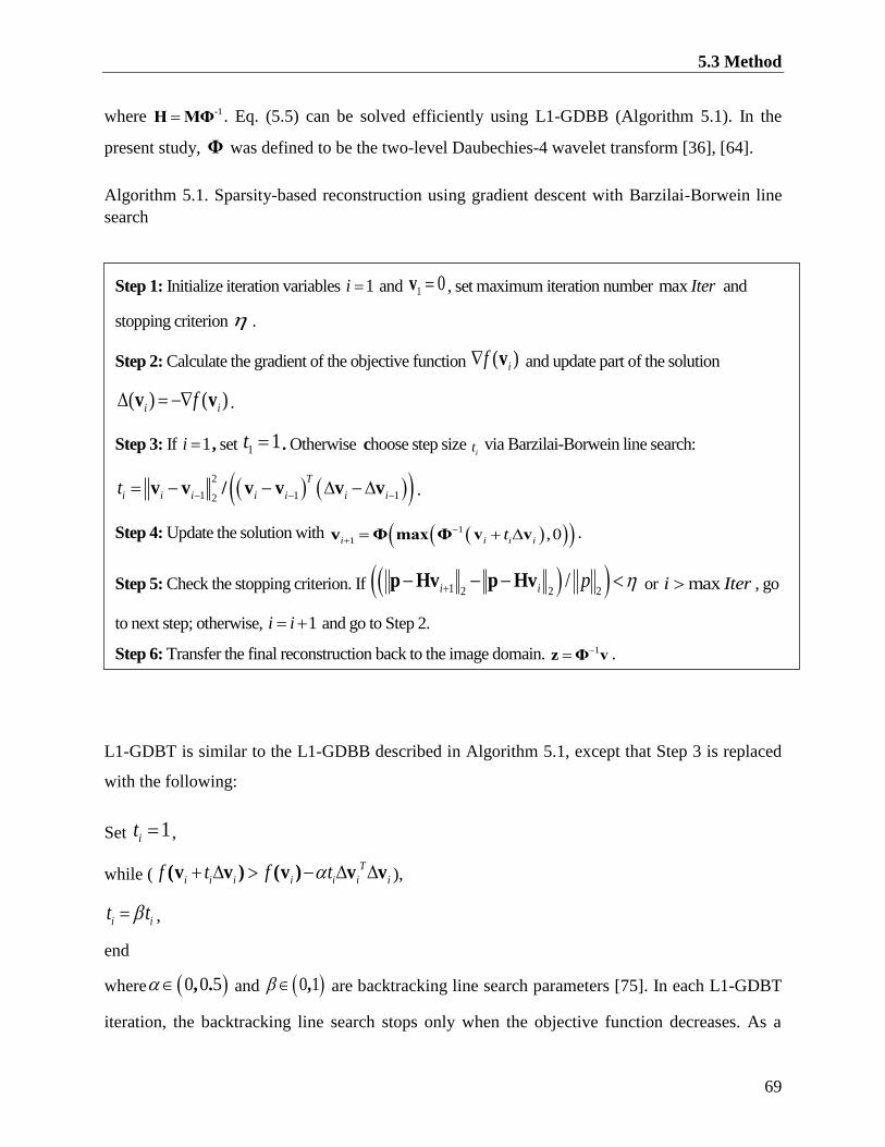
5.3 Method
69
where 1 -Η MΦ . Eq. (5.5) can be solved efficiently using L1-GDBB (Algorithm 5.1). In the
present study, Φ was defined to be the two-level Daubechies-4 wavelet transform [36], [64].
Algorithm 5.1. Sparsity-based reconstruction using gradient descent with Barzilai-Borwein line
search
L1-GDBT is similar to the L1-GDBB described in Algorithm 5.1, except that Step 3 is replaced
with the following:
Set 1i
t ,
while (T
i i i i i i if t f t (v v ) (v ) v v ),
i it t ,
end
where 0 0 5 , . and 0 1 , are backtracking line search parameters [75]. In each L1-GDBT
iteration, the backtracking line search stops only when the objective function decreases. As a
Step 1: Initialize iteration variables 1i and 1 0v , set maximum iteration number max Iter and
stopping criterion .
Step 2: Calculate the gradient of the objective function ( )if v and update part of the solution
( ) ( )i if v v .
Step 3: If 1i , set 11t . Otherwise choose step size
it via Barzilai-Borwein line search:
2
1 1 12
T
i i i i i i it
v v / v v v v .
Step 4: Update the solution with 1
1 ,0i i i it
v Φ max Φ v v .
Step 5: Check the stopping criterion. If 1 2 2 2/i i p p Hv p Hv or maxi Iter , go
to next step; otherwise, 1i i and go to Step 2.
Step 6: Transfer the final reconstruction back to the image domain. 1z Φ v .
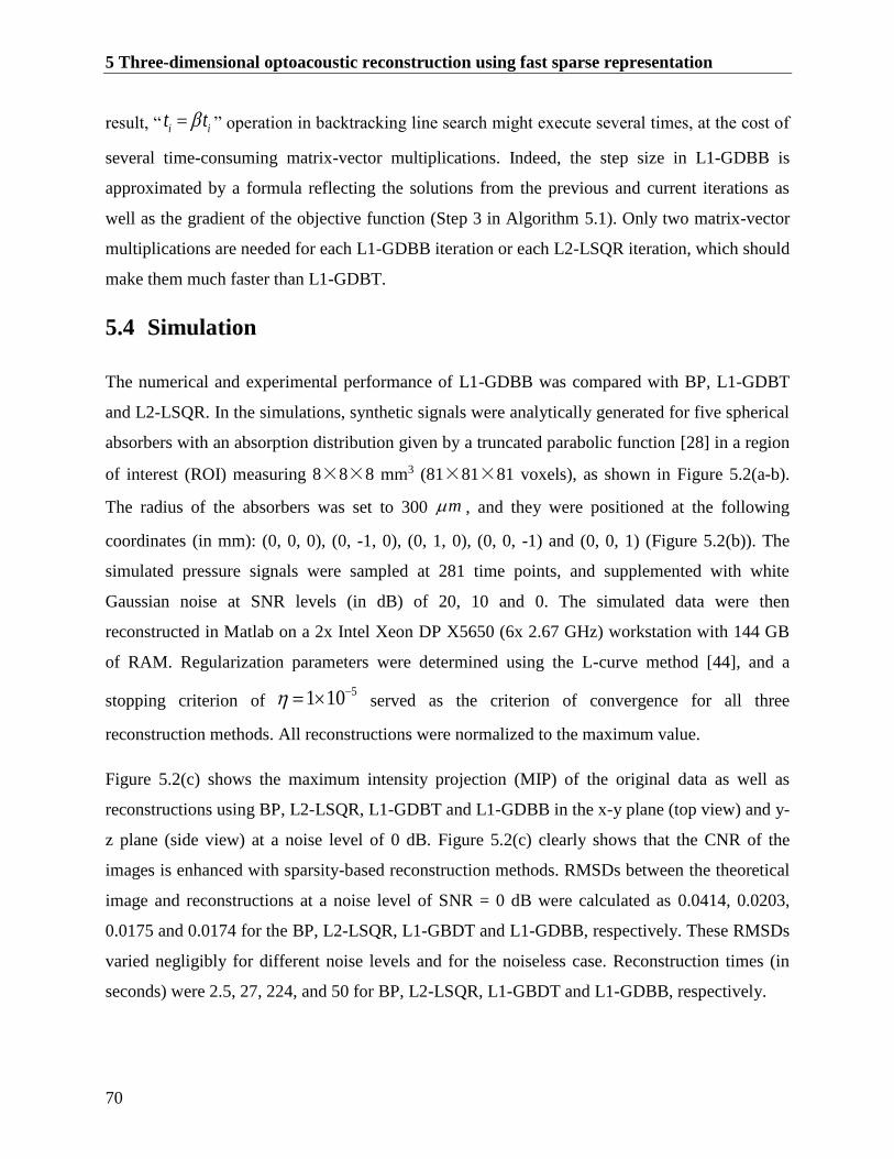
5 Three-dimensional optoacoustic reconstruction using fast sparse representation
70
result, “ i it t ” operation in backtracking line search might execute several times, at the cost of
several time-consuming matrix-vector multiplications. Indeed, the step size in L1-GDBB is
approximated by a formula reflecting the solutions from the previous and current iterations as
well as the gradient of the objective function (Step 3 in Algorithm 5.1). Only two matrix-vector
multiplications are needed for each L1-GDBB iteration or each L2-LSQR iteration, which should
make them much faster than L1-GDBT.
5.4 Simulation
The numerical and experimental performance of L1-GDBB was compared with BP, L1-GDBT
and L2-LSQR. In the simulations, synthetic signals were analytically generated for five spherical
absorbers with an absorption distribution given by a truncated parabolic function [28] in a region
of interest (ROI) measuring 8×8×8 mm3 (81×81×81 voxels), as shown in Figure 5.2(a-b).
The radius of the absorbers was set to 300 m , and they were positioned at the following
coordinates (in mm): (0, 0, 0), (0, -1, 0), (0, 1, 0), (0, 0, -1) and (0, 0, 1) (Figure 5.2(b)). The
simulated pressure signals were sampled at 281 time points, and supplemented with white
Gaussian noise at SNR levels (in dB) of 20, 10 and 0. The simulated data were then
reconstructed in Matlab on a 2x Intel Xeon DP X5650 (6x 2.67 GHz) workstation with 144 GB
of RAM. Regularization parameters were determined using the L-curve method [44], and a
stopping criterion of 51 10 served as the criterion of convergence for all three
reconstruction methods. All reconstructions were normalized to the maximum value.
Figure 5.2(c) shows the maximum intensity projection (MIP) of the original data as well as
reconstructions using BP, L2-LSQR, L1-GDBT and L1-GDBB in the x-y plane (top view) and y-
z plane (side view) at a noise level of 0 dB. Figure 5.2(c) clearly shows that the CNR of the
images is enhanced with sparsity-based reconstruction methods. RMSDs between the theoretical
image and reconstructions at a noise level of SNR = 0 dB were calculated as 0.0414, 0.0203,
0.0175 and 0.0174 for the BP, L2-LSQR, L1-GBDT and L1-GDBB, respectively. These RMSDs
varied negligibly for different noise levels and for the noiseless case. Reconstruction times (in
seconds) were 2.5, 27, 224, and 50 for BP, L2-LSQR, L1-GBDT and L1-GDBB, respectively.
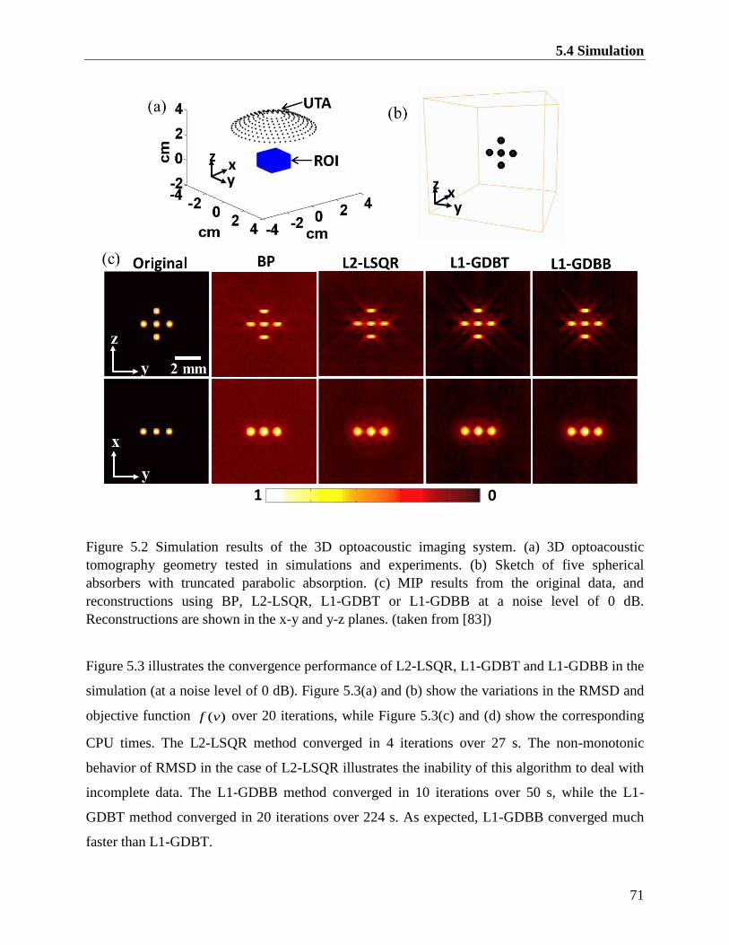
5.4 Simulation
71
Figure 5.2 Simulation results of the 3D optoacoustic imaging system. (a) 3D optoacoustic
tomography geometry tested in simulations and experiments. (b) Sketch of five spherical
absorbers with truncated parabolic absorption. (c) MIP results from the original data, and
reconstructions using BP, L2-LSQR, L1-GDBT or L1-GDBB at a noise level of 0 dB.
Reconstructions are shown in the x-y and y-z planes. (taken from [83])
Figure 5.3 illustrates the convergence performance of L2-LSQR, L1-GDBT and L1-GDBB in the
simulation (at a noise level of 0 dB). Figure 5.3(a) and (b) show the variations in the RMSD and
objective function ( )f v over 20 iterations, while Figure 5.3(c) and (d) show the corresponding
CPU times. The L2-LSQR method converged in 4 iterations over 27 s. The non-monotonic
behavior of RMSD in the case of L2-LSQR illustrates the inability of this algorithm to deal with
incomplete data. The L1-GDBB method converged in 10 iterations over 50 s, while the L1-
GDBT method converged in 20 iterations over 224 s. As expected, L1-GDBB converged much
faster than L1-GDBT.

5 Three-dimensional optoacoustic reconstruction using fast sparse representation
72
Figure 5.3 Comparison of convergence performance of simulated reconstructions at a noise level
of 0 dB using L2-LSQR, L1-GDBT or L1-GDBB. Variations in RMSD and objective function
are depicted as a function of (a-b) iteration number and (c-d) CPU time. (taken from [83])
Figure 5.4(a) shows two sets of slices (single plane) of the original data in planes of z=0 (top row)
and y=0 (bottom row), as well as the corresponding reconstructions obtained using BP, L2-
LSQR, L1-GDBT or L1-GDBB. Comparison of the two trapezoidal regions within dashed lines
in the reconstructions generated using L2-LSQR, L1-GDBT or L1-GDBB shows that L1-norm
based regularization methods give far fewer artifacts than L2-LSQR. This corroborated the MIP
results in Figure 5.2(c). Figure 5.4(b) shows the line profiles of the original data and three
reconstructions along Lines 1 indicated in Figure 5.4(a). Comparison of the line profiles of Line
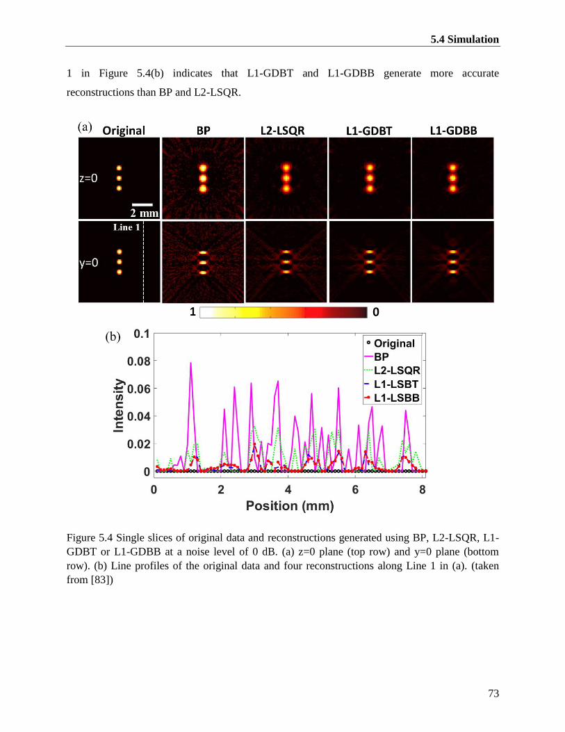
5.4 Simulation
73
1 in Figure 5.4(b) indicates that L1-GDBT and L1-GDBB generate more accurate
reconstructions than BP and L2-LSQR.
Figure 5.4 Single slices of original data and reconstructions generated using BP, L2-LSQR, L1-
GDBT or L1-GDBB at a noise level of 0 dB. (a) z=0 plane (top row) and y=0 plane (bottom
row). (b) Line profiles of the original data and four reconstructions along Line 1 in (a). (taken
from [83])
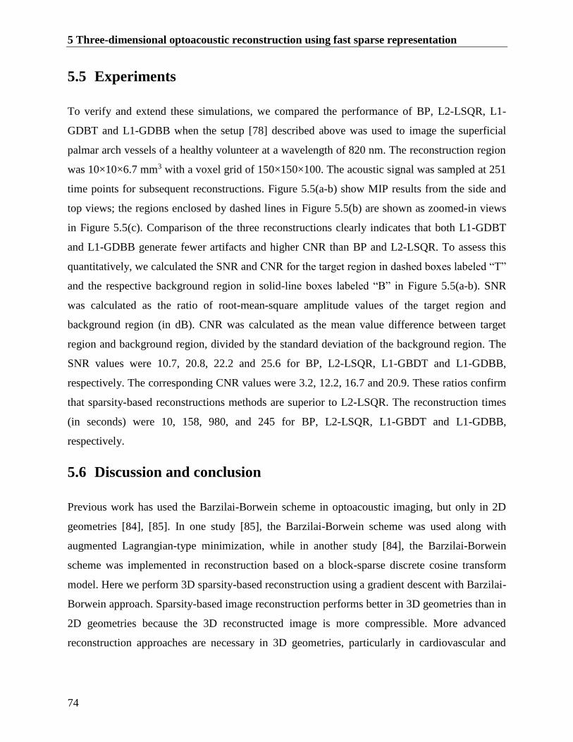
5 Three-dimensional optoacoustic reconstruction using fast sparse representation
74
5.5 Experiments
To verify and extend these simulations, we compared the performance of BP, L2-LSQR, L1-
GDBT and L1-GDBB when the setup [78] described above was used to image the superficial
palmar arch vessels of a healthy volunteer at a wavelength of 820 nm. The reconstruction region
was 10×10×6.7 mm3 with a voxel grid of 150×150×100. The acoustic signal was sampled at 251
time points for subsequent reconstructions. Figure 5.5(a-b) show MIP results from the side and
top views; the regions enclosed by dashed lines in Figure 5.5(b) are shown as zoomed-in views
in Figure 5.5(c). Comparison of the three reconstructions clearly indicates that both L1-GDBT
and L1-GDBB generate fewer artifacts and higher CNR than BP and L2-LSQR. To assess this
quantitatively, we calculated the SNR and CNR for the target region in dashed boxes labeled “T”
and the respective background region in solid-line boxes labeled “B” in Figure 5.5(a-b). SNR
was calculated as the ratio of root-mean-square amplitude values of the target region and
background region (in dB). CNR was calculated as the mean value difference between target
region and background region, divided by the standard deviation of the background region. The
SNR values were 10.7, 20.8, 22.2 and 25.6 for BP, L2-LSQR, L1-GBDT and L1-GDBB,
respectively. The corresponding CNR values were 3.2, 12.2, 16.7 and 20.9. These ratios confirm
that sparsity-based reconstructions methods are superior to L2-LSQR. The reconstruction times
(in seconds) were 10, 158, 980, and 245 for BP, L2-LSQR, L1-GBDT and L1-GDBB,
respectively.
5.6 Discussion and conclusion
Previous work has used the Barzilai-Borwein scheme in optoacoustic imaging, but only in 2D
geometries [84], [85]. In one study [85], the Barzilai-Borwein scheme was used along with
augmented Lagrangian-type minimization, while in another study [84], the Barzilai-Borwein
scheme was implemented in reconstruction based on a block-sparse discrete cosine transform
model. Here we perform 3D sparsity-based reconstruction using a gradient descent with Barzilai-
Borwein approach. Sparsity-based image reconstruction performs better in 3D geometries than in
2D geometries because the 3D reconstructed image is more compressible. More advanced
reconstruction approaches are necessary in 3D geometries, particularly in cardiovascular and
5.6 Discussion and conclusion
75
neurological imaging, which may help reduce the artifacts arising from insufficient data (as
shown in Figure 5.2, Figure 5.4 and Figure 5.5).
Figure 5.5 Reconstructions of experimental data using BP, L2-LSQR, L1-GDBT and L1-GDBB.
(a-b) MIP results (side and top views) of reconstructions of experimental data using BP, L2-
LSQR, L1-GDBT and L1-GDBB. (c) Zoomed-in images of the top-view MIP region enclosed in
the dot-dashed box in (b). The corresponding region for each reconstruction is shown, even
though the box is drawn only for BP. The regions labeled “T” and “B” served as target and
background regions, respectively, for calculating SNR and CNR. (taken from [83])
Taken together, our results indicate that the two sparsity-based methods perform well and generate far
fewer artifacts and higher CNR than BP reconstruction and commonly-used iterative reconstruction
approaches based on L2-norm regularization. Specifically, both L1- GDBT and L1-GDBB performed
better than BP and L2-LSQR in simulation and experiments, and L1-GDBB showed a 4-fold faster
computational time than L1-GDBT. The computational complexity at each iteration of the L1-GDBT and
5 Three-dimensional optoacoustic reconstruction using fast sparse representation
76
L1-GDBB algorithms are 2
itN N and N , where N represents the size of image and itN is the
number of backtracking line search iterations. This substantial gain in reconstruction quality with L1-
GDBB with respect to L2-LSQR comes with only a moderate 55% increase in CPU time. Short
reconstruction time is essential in practical applications, particularly when processing large datasets, such
as in biomedical research. Image reconstruction can be further accelerated through parallel
implementations of the algorithms in a graphics processing unit (GPU). For example, efficient GPU
implementation of the matrix-vector multiplications in iterative inversions can significantly accelerate L2-
LSQR-based reconstruction, even allowing real-time reconstruction with a 2D model [86]. Thereby,
similar implementations for a 3D optoacoustic model combined with the L1-GDBB method described
here may lead to a highly practical and accurate approach in the future.
The L1-GDBB method can become especially beneficial in the case of incomplete tomographic
data. Reasons for this incompleteness may be the restricted accessibility to surrounding positions
of the sample or technological constraints limiting the number of channels that can be acquired
per laser pulse, e.g. in dynamic imaging applications. A particularly important example of
insufficient data is limited-view acquisition, when acoustic signals are collected only over a
limited angle. Limited-view acquisition is particularly important for optoacoustic clinical
translation as hand-held or endoscopic probes cannot fully enclose the imaged tissue. In this case,
proper regularization can also enhance the CNR of the images [74] and reduce sharp artifacts
corresponding to the edges of the detection arc [87]. Even with good regularization, structures in
certain orientations may not be visualized well in limited-view acquisitions, which can be
corrected using other approaches [88]–[90].
In conclusion, the reconstruction approach suggested here can greatly impact the resolution,
contrast and overall quality of the optoacoustic images rendered with currently-used 3D
tomographic systems. The proposed method may become the method of choice in many practical
cases.
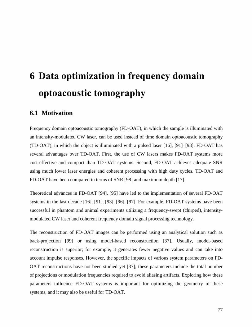
77
6 Data optimization in frequency domain
optoacoustic tomography
6.1 Motivation
Frequency domain optoacoustic tomography (FD-OAT), in which the sample is illuminated with
an intensity-modulated CW laser, can be used instead of time domain optoacoustic tomography
(TD-OAT), in which the object is illuminated with a pulsed laser [16], [91]–[93]. FD-OAT has
several advantages over TD-OAT. First, the use of CW lasers makes FD-OAT systems more
cost-effective and compact than TD-OAT systems. Second, FD-OAT achieves adequate SNR
using much lower laser energies and coherent processing with high duty cycles. TD-OAT and
FD-OAT have been compared in terms of SNR [98] and maximum depth [17].
Theoretical advances in FD-OAT [94], [95] have led to the implementation of several FD-OAT
systems in the last decade [16], [91], [93], [96], [97]. For example, FD-OAT systems have been
successful in phantom and animal experiments utilizing a frequency-swept (chirped), intensity-
modulated CW laser and coherent frequency domain signal processing technology.
The reconstruction of FD-OAT images can be performed using an analytical solution such as
back-projection [99] or using model-based reconstruction [37]. Usually, model-based
reconstruction is superior; for example, it generates fewer negative values and can take into
account impulse responses. However, the specific impacts of various system parameters on FD-
OAT reconstructions have not been studied yet [37]; these parameters include the total number
of projections or modulation frequencies required to avoid aliasing artifacts. Exploring how these
parameters influence FD-OAT systems is important for optimizing the geometry of these
systems, and it may also be useful for TD-OAT.

6 Data optimization in frequency domain optoacoustic tomography
78
In this chapter, model-based FD-OAT reconstruction is explored using measured optoacoustic
amplitude and phase at multiple discrete frequencies. The Nyquist-Shannon theorem is used to
identify a linear relationship linking the number of projections, reconstruction dimensions/field
of view, the number of modulation frequencies and the speed of sound for FD-OAT
reconstruction. This formula is validated in numerical simulations. Another formula is derived
indicating the minimum number of frequencies needed for adequate reconstruction. Finally
condition number of the forward model matrix is studied to reveal the influence of the
parameters in FD-OAT.
6.2 Method
Model-based reconstruction in FD-OAT is based on the equation [36], [37]
p M z , (6.1)
where p is the vector of the measured complex signals and z is the vector denoting the
object. M is the forward model matrix, which is given as
n m p qi c r r
nm n p q
m p q
e
r r
,/
, ,
,
M (6.2)
where 1i , n is the angular frequency, c is the speed of sound, ,p q
r is the Cartesian
coordinates, and mr is the transducer position.
The complex forward model matrix M and measurements p can be re-expressed in real
number format for the following inversion:
p M z , (6.3)
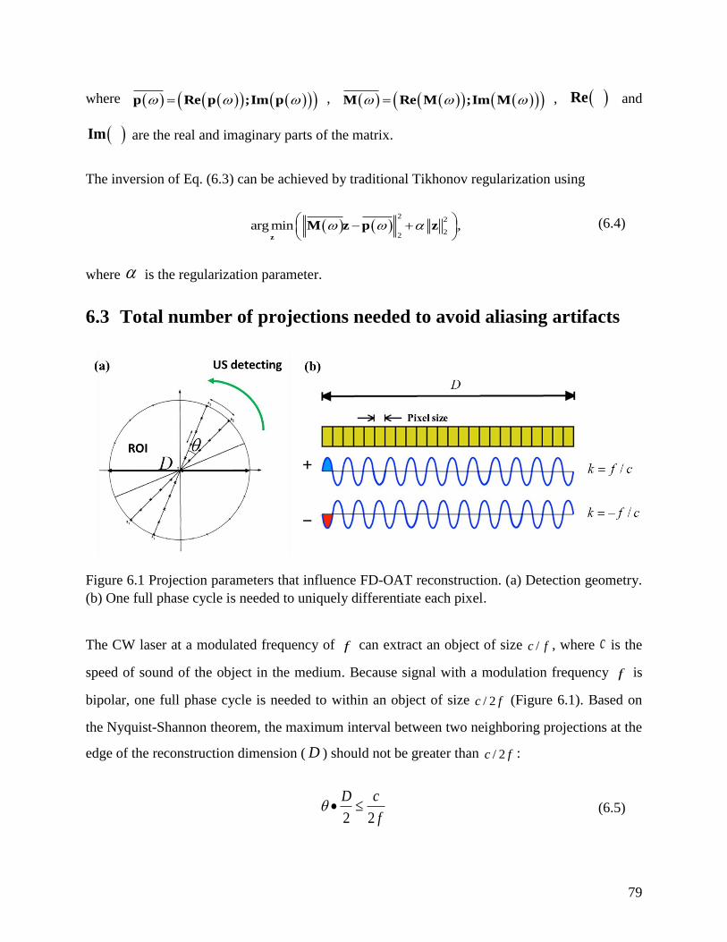
79
where p Re p ;Im p , M Re M ;Im M , Re and
Im are the real and imaginary parts of the matrix.
The inversion of Eq. (6.3) can be achieved by traditional Tikhonov regularization using
2
2
22
arg min ,
z
M z p z (6.4)
where is the regularization parameter.
6.3 Total number of projections needed to avoid aliasing artifacts
Figure 6.1 Projection parameters that influence FD-OAT reconstruction. (a) Detection geometry.
(b) One full phase cycle is needed to uniquely differentiate each pixel.
The CW laser at a modulated frequency of f can extract an object of size /c f , where c is the
speed of sound of the object in the medium. Because signal with a modulation frequency f is
bipolar, one full phase cycle is needed to within an object of size / 2c f (Figure 6.1). Based on
the Nyquist-Shannon theorem, the maximum interval between two neighboring projections at the
edge of the reconstruction dimension ( D ) should not be greater than / 2c f :
2 2
D c
f • (6.5)
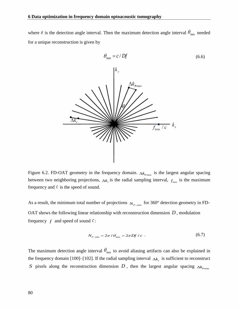
6 Data optimization in frequency domain optoacoustic tomography
80
where is the detection angle interval. Then the maximum detection angle interval max needed
for a unique reconstruction is given by
max /c Df (6.6)
Figure 6.2. FD-OAT geometry in the frequency domain. maxk is the largest angular spacing
between two neighboring projections, rk is the radial sampling interval,
maxf is the maximum
frequency and c is the speed of sound.
As a result, the minimum total number of projections _minP
N for 360° detection geometry in FD-
OAT shows the following linear relationship with reconstruction dimension D , modulation
frequency f and speed of sound c :
_min max
2 2P
N Df c / / . (6.7)
The maximum detection angle interval max to avoid aliasing artifacts can also be explained in
the frequency domain [100]–[102]. If the radial sampling interval rk is sufficient to reconstruct
S pixels along the reconstruction dimension D , then the largest angular spacing maxk
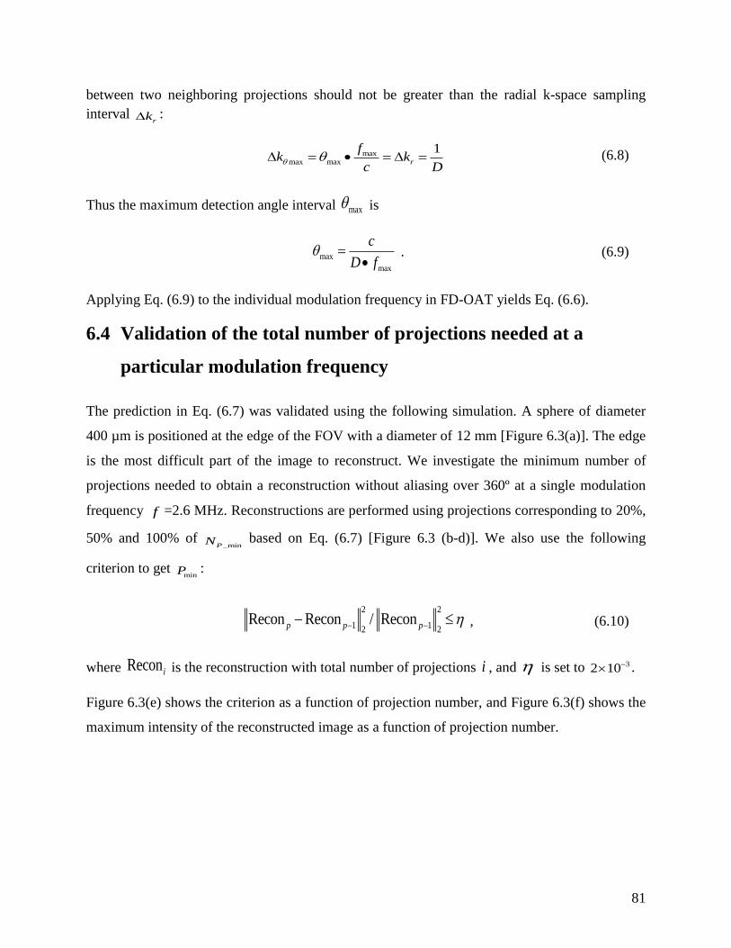
81
between two neighboring projections should not be greater than the radial k-space sampling
interval rk :
maxmax max
1r
fk k
c D • (6.8)
Thus the maximum detection angle interval max is
max
max
c
D f
• . (6.9)
Applying Eq. (6.9) to the individual modulation frequency in FD-OAT yields Eq. (6.6).
6.4 Validation of the total number of projections needed at a
particular modulation frequency
The prediction in Eq. (6.7) was validated using the following simulation. A sphere of diameter
400 µm is positioned at the edge of the FOV with a diameter of 12 mm [Figure 6.3(a)]. The edge
is the most difficult part of the image to reconstruct. We investigate the minimum number of
projections needed to obtain a reconstruction without aliasing over 360º at a single modulation
frequency f =2.6 MHz. Reconstructions are performed using projections corresponding to 20%,
50% and 100% of _minP
N based on Eq. (6.7) [Figure 6.3 (b-d)]. We also use the following
criterion to get min
P :
2 2
1 12 2Recon Recon / Reconp p p , (6.10)
where Reconi is the reconstruction with total number of projections i , and is set to 32 10 .
Figure 6.3(e) shows the criterion as a function of projection number, and Figure 6.3(f) shows the
maximum intensity of the reconstructed image as a function of projection number.
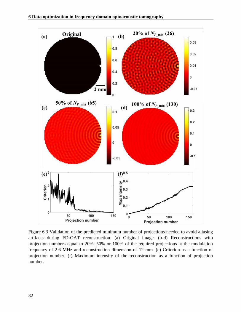
6 Data optimization in frequency domain optoacoustic tomography
82
Figure 6.3 Validation of the predicted minimum number of projections needed to avoid aliasing
artifacts during FD-OAT reconstruction. (a) Original image. (b-d) Reconstructions with
projection numbers equal to 20%, 50% or 100% of the required projections at the modulation
frequency of 2.6 MHz and reconstruction dimension of 12 mm. (e) Criterion as a function of
projection number. (f) Maximum intensity of the reconstruction as a function of projection
number.
6.5 Total number of modulation frequencies needed for even sampling
83
6.5 Total number of modulation frequencies needed for even
sampling
A total number of modulation frequencies FN is generated with an even sampling (ES) pattern
over the bandwidth max0, f . The individual modulation frequency ES
if is given as [37]
ES max
i
Ff i f N • / . (6.11)
To ensure a unique reconstruction, the total number of independent measurements should not
more than twice of the total number of pixels. The sum of projections [1,..., FP P ] at the
FN
modulation frequencies can be described as
2
max1 2 1
max
2 2... ... 2*
2 4 / 2
FF F
f ND D DP P P f f
c c f c
•
. (6.12)
In this case, the minimum total number of modulation frequencies _ minFN for the reconstruction
dimension ( D ) with the highest frequency maxf should be
_ min max2 /FN D f c • . (6.13)
6.6 Analysis the measurements optimization with condition number
of forward matrix
The condition number of the forward model matrix in FD-OAT indicates the ability of how good
the original image can be reconstructed [37]. Using simulations, we investigate how
reconstruction quality changes when FN and PN fall below the respective _ minFN and
_minPN
thresholds derived using the Eq. (6.13) and Eq. (6.7). This validates our mathematical approach,
and it also provides a rational basis for assessing reconstruction quality when the numbers of
projections and/or modulation frequencies are too few. Simulations were performed using the
following parameters: detection angle, 180°; reconstruction grid, 60 60; reconstruction
resolution, 200 µm; and speed of sound, 1500 m/s. In this case, _ minFN is 60, and
_minPN for
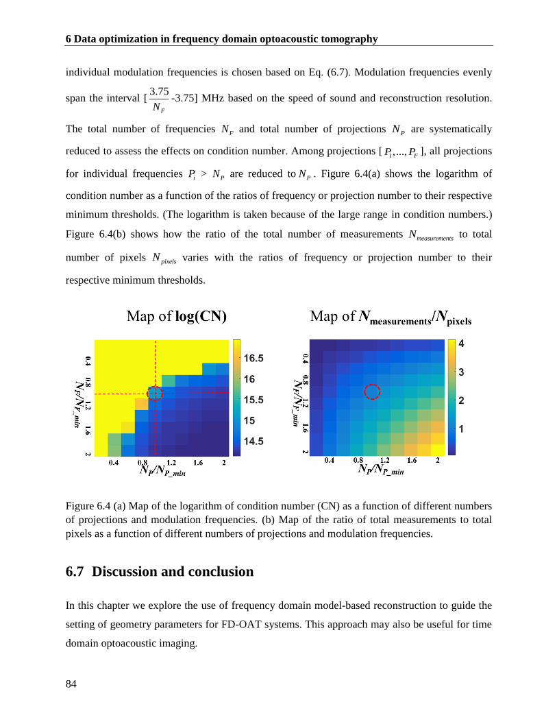
6 Data optimization in frequency domain optoacoustic tomography
84
individual modulation frequencies is chosen based on Eq. (6.7). Modulation frequencies evenly
span the interval [3.75
FN-3.75] MHz based on the speed of sound and reconstruction resolution.
The total number of frequencies FN and total number of projections PN are systematically
reduced to assess the effects on condition number. Among projections [1,..., FP P ], all projections
for individual frequencies iP > PN are reduced to PN . Figure 6.4(a) shows the logarithm of
condition number as a function of the ratios of frequency or projection number to their respective
minimum thresholds. (The logarithm is taken because of the large range in condition numbers.)
Figure 6.4(b) shows how the ratio of the total number of measurements measurementsN to total
number of pixels pixelsN varies with the ratios of frequency or projection number to their
respective minimum thresholds.
Figure 6.4 (a) Map of the logarithm of condition number (CN) as a function of different numbers
of projections and modulation frequencies. (b) Map of the ratio of total measurements to total
pixels as a function of different numbers of projections and modulation frequencies.
6.7 Discussion and conclusion
In this chapter we explore the use of frequency domain model-based reconstruction to guide the
setting of geometry parameters for FD-OAT systems. This approach may also be useful for time
domain optoacoustic imaging.
6.7 Discussion and conclusion
85
Previous frequency domain optoacoustic imaging approaches defined a “global” projection
number that was the same for all modulation frequencies within the frequency band. The
approach proposed here, based on the Nyquist theorem, uses an equation that determines the
minimum projection number separately for each frequency in the band, in order to ensure a
unique reconstruction. This equation is validated with a numerical simulation for different
frequencies and different reconstruction image sizes. This equation is validated in the case of
noiseless data. In the presence of noise, the number of required projections may be greater than
what the equation indicates.
We also analyzed the influence of the number of frequencies sampled within a bandwidth on the
resulting reconstruction. The minimum number of frequencies needed to achieve a unique
reconstruction in FD-OAT can be calculated analytically. This approach is validated by
computing the condition number of the frequency domain model matrix for different numbers of
modulation frequencies within the bandwidth.
The condition number of the frequency domain model matrix correlates with the robustness of
the reconstruction to input error or noise. Figure 6.4(a) shows that when the modulation
frequency number and projection number are both insufficient, the condition number is too high,
indicating that it is impossible to get a unique reconstruction for the general case. Conversely,
when the modulation frequency number and projection number are both sufficient, a unique
reconstruction is possible in all cases. In situations when one or the other number is insufficient,
the other parameter can be manipulated to compensate. Thus it may be useful to perform
condition number analysis for FD-OAT in order to optimize the procedure when data limitations
are likely. Such analysis may be useful even when sufficient frequencies and projections are
available, since it can define the minimum dataset needed for adequate reconstruction, allowing
data elimination for quality control reasons without jeopardizing the reconstruction.

6 Data optimization in frequency domain optoacoustic tomography
86
87
7 Conclusion and outlook
7.1 Conclusive remarks
Reconstruction is an essential process for optoacoustic tomography. Accurate reconstruction
permits visualization of complex anatomical structures, and it facilitates subsequent multispectral
analysis. The present work introduced model-based acoustic inversion methods for various
optoacoustic tomography systems.
First, a method for accelerating optoacoustic reconstruction and performing system analysis
using a wavelet-packet framework is proposed and tested with an optoacoustic system involving
a single-element transducer. The spatial impulse response of the transducer is incorporated into
the optoacoustic system model matrix for subsequent inversion. Transferring the model matrix
and the optoacoustic signal into the wavelet domain significantly accelerates the reconstruction,
which enables parallel TSVD inversion on a much smaller scale. In the event that the
optoacoustic model matrix is too big for SVD analysis, the condition number can be calculated
for smaller submatrices generated after wavelet packet decomposition.
Next, a sparsity-based reconstruction is developed for a cross-sectional optoacoustic system with
a focused transducer array. A cost function is used that includes the L1 norm of the image in
sparse representation and a total variation term. The minimization process is implemented with
gradient descent with backtracking line search. Model-based sparsity-based inversion performs
better than conventional Tikhonov regularization and back-projection reconstruction for
reconstructing numerical and experimental datasets involving full-view and limited-view
geometries, giving sharper images and weaker streak artifacts.
7 Conclusion and outlook
88
Sparsity-based reconstruction is then adapted to 3D geometries, since ultrasound waves in
optoacoustics propagate in all directions and reconstructed images are more compressible in 3D.
To accelerate reconstruction, Barzilai-Borwein line search is used to determine analytically the
step size for each iteration of gradient descent. The proposed method offers 4-fold faster
reconstruction than the previously reported L1-norm regularized reconstruction based on
gradient descent with backtracking line search. Moreover, the new algorithm provides higher-
quality images with fewer artifacts than the L2-norm regularized reconstruction and the back-
projection reconstruction.
Finally, optoacoustic reconstruction is studied in the frequency domain. The Nyquist-Shannon
theorem is applied to uncover a linear relationship among projection number, reconstruction
dimensions, modulation frequency and speed of sound to obtain a unique reconstruction. .We
also get a formula to get the minimum demand of the frequencies needed. Analysis of forward
model matrix characteristics, e.g. condition number, which is typical in time domain
optoacoustic tomography, is extended here to the frequency domain to reveal inherent
reconstruction properties.
7.2 Outlook and future directions
One direction is to accelerate the reconstruction with the wavelet packet framework utilizing
model matrix sparsity. Extending the 2D algorithm presented here to 3D will require overcoming
several challenges. One is to reduce the memory of the large model matrix in 3D as much as
possible before wavelet packet decomposition. Another is to deal with the expected complexity
of inverting with wavelet packets in the case of limited-view geometry.
Sparsity-based optoacoustic reconstructions are shown here to provide superior image quality
over existing reconstruction algorithms. However, sparsity-based reconstructions in this thesis
are implemented on a CPU and require a certain amount of computational time. Short
reconstruction time is essential in practical applications, particularly for large datasets. Image
reconstruction can be further accelerated through parallel implementations of the algorithms in a
graphics processing unit (GPU). For example, efficient GPU implementation of the matrix-
vector multiplications in iterative inversions can significantly accelerate L2-norm based
reconstruction, even allowing real-time reconstruction with a 2D model [86]. Therefore, similar
7.2 Outlook and future directions
89
implementations for a 3D optoacoustic model combined with the sparsity-based method
described here may lead to a tool that is both accurate and practical. Another direction is to study
the random selection on projections under the sparsity-based reconstruction framework to reduce
the measurements and reconstruction time.
Finally, frequency domain optoacoustic tomography is analyzed here as an alternative to the
same technique in the time domain. Frequency domain optoacoustic tomography offers the
freedom of selectively exciting the object with a certain frequency band or even single
frequencies, depending on absorber size (reconstruction image resolution). Sampling pattern is
an interesting topic in frequency domain optoacoustic tomography reconstruction. In addition,
frequency domain model-based reconstruction can be used to study sparsity-based reconstruction
methods involving single modulation frequencies, which may be useful for understanding and
improving time domain sparsity-based optoacoustic reconstruction. It may be possible to further
improve frequency domain model-based reconstruction algorithms using fast Fourier
transformation.

7 Conclusion and outlook
90
91
Publications list
1. Yiyong Han, Lu Ding, Xosé Luis Deán Ben, Daniel Razansky, Jaya Prakash, Vasilis
Ntziachristos. Three-dimensional optoacoustic reconstruction using fast sparse representation.
Optics Letters 42(5), 979-982 (2017)
2. Yiyong Han, Vasilis Ntziachristos, Amir Rosenthal. Optoacoustic image reconstruction
and system analysis for finite-aperture detectors under the wavelet-packet framework. Journal of
Biomedical Optics 21(1), 016002 (2016)
3. Yiyong Han, Stratis Tzoumas, Antonio Nunes, Vasilis Ntziachristos, Amir Rosenthal.
Sparsity-based acoustic inversion in cross-sectional multi-scale optoacoustic imaging. Medical
Physics 42(9), 5444-5452 (2015)

Publications list
92
93
Bibliography
[1] V. Ntziachristos, “Going deeper than microscopy: the optical imaging frontier in biology.,”
Nat. Methods, vol. 7, no. 8, pp. 603–614, 2010.
[2] L. V. Wang and S. Hu, “Photoacoustic Tomography: In Vivo Imaging from Organelles to
Organs,” Science, vol. 335, no. 6075, pp. 1458–1462, Mar. 2012.
[3] C. Li and L. V Wang, “Photoacoustic tomography and sensing in biomedicine,” Phys.
Med. Biol., vol. 54, no. 19, pp. R59–R97, 2009.
[4] P. Beard, “Biomedical photoacoustic imaging.,” Interface Focus, vol. 1, no. 4, pp. 602–31,
2011.
[5] M. Xu and L. V. Wang, “Photoacoustic imaging in biomedicine,” Rev. Sci. Instrum., vol.
77, no. 4, pp. 1–22, 2006.
[6] D. Razansky, A. Buehler, and V. Ntziachristos, “Volumetric real-time multispectral
optoacoustic tomography of biomarkers.,” Nat. Protoc., vol. 6, no. 8, pp. 1121–29, 2011.
[7] G. J. Diebold, T. Sun, and M. I. Khan, “Photoacoustic monopole radiation in one, two,
and three dimensions,” Phys. Rev. Lett., vol. 67, no. 24, pp. 3384–3387, 1991.
[8] Lihong V. Wang, Photoacoustic Imaging and Spectroscopy. Boca Raton, Florida: CRC
Press, 2009.
[9] Lihong V. Wang and Hsin i Wu, Biomedical Optics. Hoboken, New Jersey: John Wiley &
Sons, 2007.
[10] A. Rosenthal, V. Ntziachristos, and D. Razansky, “Acoustic Inversion in Optoacoustic
Tomography: A Review,” Curr. Med. Imaging Rev., vol. 9, no. 4, pp. 318–336, 2013.
[11] J. Yao and L. V. Wang, “Photoacoustic microscopy,” Laser Photon. Rev., vol. 7, no. 5, pp.
758–778, 2013.
Bibliography
94
[12] J. Yao and L. V. Wang, “Sensitivity of photoacoustic microscopy,” Photoacoustics, vol. 2,
no. 2, pp. 87–101, 2014.
[13] V. Ntziachristos and D. Razansky, “Molecular imaging by means of multispectral
optoacoustic tomography (MSOT),” Chem. Rev., vol. 110, no. 5, pp. 2783–2794, 2010.
[14] D. Razansky, M. Distel, C. Vinegoni, R. Ma, N. Perrimon, R. W. Koster, and V.
Ntziachristos, “Multispectral opto-acoustic tomography of deep-seated fluorescent
proteins in vivo,” Nat. Photonics, vol. 3, no. 7, pp. 412–417, 2009.
[15] X. Wang, Y. Pang, G. Ku, X. Xie, G. Stoica, and L. V Wang, “Noninvasive laser-induced
photoacoustic tomography for structural and functional in vivo imaging of the brain.,” Nat.
Biotechnol., vol. 21, no. 7, pp. 803–806, 2003.
[16] S. Telenkov, A. Mandelis, B. Lashkari, and M. Forcht, “Frequency-domain
photothermoacoustics: Alternative imaging modality of biological tissues,” J. Appl. Phys.,
vol. 105, no. 10, 2009.
[17] S. a Telenkov and A. Mandelis, “Photothermoacoustic imaging of biological tissues:
maximum depth characterization comparison of time and frequency-domain
measurements.,” J. Biomed. Opt., vol. 14, no. 4, p. 44025, 2009.
[18] R. A. Kruger, “Photoacoustic ultrasound (PAUS)—Reconstruction tomography,” Med.
Phys., vol. 22, no. 10, p. 1605, 1995.
[19] M. Xu and L. V. Wang, “Universal back-projection algorithm for photoacoustic computed
tomography,” Phys. Rev. E - Stat. Nonlinear, Soft Matter Phys., vol. 71, no. 1, pp. 1–7,
2005.
[20] K. P. Koestli, M. Frenz, H. Bebie, H. P. Weber, and K. P. Köstli, “Temporal backward
projection of optoacoustic pressure transients using fourier transform methods,” Phys.
Med. Biol., vol. 46, no. 7, pp. 1863–72, 2001.
[21] Y. Xu and L. V Wang, “Time reversal and its application to tomography with diffracting
sources.,” Phys. Rev. Lett., vol. 92, no. 3, p. 33902, 2004.
[22] P. Burgholzer, G. J. Matt, M. Haltmeier, and G. Paltauf, “Exact and approximative
imaging methods for photoacoustic tomography using an arbitrary detection surface,”
Phys. Rev. E - Stat. Nonlinear, Soft Matter Phys., vol. 75, no. 4, pp. 1–10, 2007.
Bibliography
95
[23] B. E. Treeby, E. Z. Zhang, and B. T. Cox, “Photoacoustic tomography in absorbing
acoustic media using time reversal,” Inverse Probl., vol. 26, no. 11, p. 115003, 2010.
[24] A. Rosenthal, D. Razansky, and V. Ntziachristos, “Fast semi-analytical model-based
acoustic inversion for quantitative optoacoustic tomography,” IEEE Trans. Med. Imaging,
vol. 29, no. 6, pp. 1275–1285, 2010.
[25] C. G. Hoelen and F. F. de Mul, “Image reconstruction for photoacoustic scanning of tissue
structures.,” Appl. Opt., vol. 39, no. 31, pp. 5872–5883, 2000.
[26] Y. Han, V. Ntziachristos, and A. Rosenthal, “Optoacoustic image reconstruction and
system analysis for finite-aperture detectors under the wavelet-packet framework,” J.
Biomed. Opt., vol. 21, no. 1, p. 16002, Jan. 2016.
[27] A. Rosenthal, V. Ntziachristos, and D. Razansky, “Model-based optoacoustic inversion
with arbitrary-shape detectors.,” Med. Phys., vol. 38, no. 7, pp. 4285–4295, 2011.
[28] D. Queirós, X. L. Déan-Ben, A. Buehler, D. Razansky, A. Rosenthal, and V. Ntziachristos,
“Modeling the shape of cylindrically focused transducers in three-dimensional
optoacoustic tomography.,” J. Biomed. Opt., vol. 18, p. 76014, 2013.
[29] K. Wang, S. A. Ermilov, R. Su, H. P. Brecht, A. A. Oraevsky, and M. A. Anastasio, “An
imaging model incorporating ultrasonic transducer properties for three-dimensional
optoacoustic tomography,” IEEE Trans. Med. Imaging, vol. 30, no. 2, pp. 203–214, 2011.
[30] A. Buehler, A. Rosenthal, T. Jetzfellner, A. Dima, D. Razansky, and V. Ntziachristos,
“Model-based optoacoustic inversions with incomplete projection data,” Med Phys, vol.
38, no. 3, pp. 1694–1704, 2011.
[31] Y. Xu, L. V Wang, G. Ambartsoumian, and P. Kuchment, “Reconstructions in limited-
view thermoacoustic tomography.,” Med. Phys., vol. 31, no. 4, pp. 724–733, 2004.
[32] X. L. Deán-Ben, R. Ma, A. Rosenthal, V. Ntziachristos, and D. Razansky, “Weighted
model-based optoacoustic reconstruction in acoustic scattering media.,” Phys. Med. Biol.,
vol. 58, no. 16, pp. 5555–66, 2013.
[33] X. L. Deán-Ben, V. Ntziachristos, and D. Razansky, “Effects of small variations of speed
of sound in optoacoustic tomographic imaging.,” Med. Phys., vol. 41, no. 7, p. 73301,
2014.
Bibliography
96
[34] X. L. Dean-Ben, A. Buehler, V. Ntziachristos, and D. Razansky, “Accurate model-based
reconstruction algorithm for three-dimensional optoacoustic tomography,” IEEE Trans.
Med. Imaging, vol. 31, no. 10, pp. 1922–1928, 2012.
[35] X. L. Deán-Ben, V. Ntziachristos, and D. Razansky, “Acceleration of optoacoustic model-
based reconstruction using angular image discretization,” IEEE Trans. Med. Imaging, vol.
31, no. 5, pp. 1154–1162, 2012.
[36] J. Provost and F. Lesage, “The application of compressed sensing for photo-acoustic
tomography,” IEEE Trans. Med. Imaging, vol. 28, no. 4, pp. 585–594, 2009.
[37] P. Mohajerani, S. Kellnberger, and V. Ntziachristos, “Frequency domain optoacoustic
tomography using amplitude and phase,” Photoacoustics, vol. 2, no. 3, pp. 111–118, 2014.
[38] K. Wang, R. Su, A. a Oraevsky, and M. a Anastasio, “Investigation of iterative image
reconstruction in three-dimensional optoacoustic tomography,” Phys. Med. Biol., vol. 57,
no. 17, pp. 5399–5423, 2012.
[39] F. A. Duck, Physical Properties of Tissue: A Comprehensive Reference Book. London:
Academic Press, 1990.
[40] P. Laugier and G. Haïat, Bone Quantitative Ultrasound. Dordrecht: Springer Netherlands,
2011.
[41] B. T. Cox, S. Kara, S. R. Arridge, and P. C. Beard, “K-Space Propagation Models for
Acoustically Heterogeneous Media: Application To Biomedical Photoacoustics.,” J.
Acoust. Soc. Am., vol. 121, no. 6, pp. 3453–3464, 2007.
[42] L. V Wang and X. Yang, “Boundary conditions in photoacoustic tomography and image
reconstruction,” J. Biomed. Opt., vol. 12, no. 1, p. 14027, 2007.
[43] K. P. Köstli and P. C. Beard, “Two-dimensional photoacoustic imaging by use of Fourier-
transform image reconstruction and a detector with an anisotropic response.,” Appl. Opt.,
vol. 42, no. 10, pp. 1899–908, 2003.
[44] P. C. Hansen, “The L-Curve and its Use in the Numerical Treatment of Inverse Problems,”
Comput. Inverse Probl. Electrocardiology, ed. P. Johnston, Adv. Comput. Bioeng., vol. 4,
pp. 119–142, 2000.
Bibliography
97
[45] K. Wang, R. W. Schoonover, R. Su, A. Oraevsky, and M. A. Anastasio, “Discrete imaging
models for three-dimensional optoacoustic tomography using radially symmetric
expansion functions,” IEEE Trans. Med. Imaging, vol. 33, no. 5, pp. 1180–1193, 2014.
[46] T. Jetzfellner, A. Rosenthal, K. H. Englmeier, A. Dima, M. N. A. Caballero, D. Razansky,
and V. Ntziachristos, “Interpolated model-matrix optoacoustic tomography of the mouse
brain,” Appl. Phys. Lett., vol. 98, no. 16, pp. 1–4, 2011.
[47] C. Lutzweiler, X. L. Dean-Ben, and D. Razansky, “Expediting model-based optoacoustic
reconstructions with tomographic symmetries.,” Med. Phys., vol. 41, p. 13302, 2014.
[48] A. Taruttis, S. Morscher, N. C. Burton, D. Razansky, and V. Ntziachristos, “Fast
multispectral optoacoustic tomography (MSOT) for dynamic imaging of pharmacokinetics
and biodistribution in multiple organs,” PLoS One, vol. 7, no. 1, p. e30491, 2012.
[49] E. Herzog, A. Taruttis, N. Beziere, A. a Lutich, and D. Razansky, “Optical imaging of
cancer heterogeneity with Multispectral,” Radiology, vol. 263, no. 2, pp. 461–468, 2012.
[50] A. Buehler, M. Kacprowicz, A. Taruttis, and V. Ntziachristos, “Real-time handheld
multispectral optoacoustic imaging.,” Opt. Lett., vol. 38, no. 9, pp. 1404–6, 2013.
[51] J. Gateau, M. A. A. Caballero, A. Dima, and V. Ntziachristos, “Three-dimensional
optoacoustic tomography using a conventional ultrasound linear detector array: whole-
body tomographic system for small animals.,” Med. Phys., vol. 40, no. 1, p. 13302, 2013.
[52] A. Rosenthal, T. Jetzfellner, D. Razansky, and V. Ntziachristos, “Efficient framework for
model-based tomographic image reconstruction using wavelet packets,” IEEE Trans. Med.
Imaging, vol. 31, no. 7, pp. 1346–1357, 2012.
[53] R. Ma, A. Taruttis, V. Ntziachristos, and D. Razansky, “Multispectral optoacoustic
tomography (MSOT) scanner for whole-body small animal imaging,” Opt. Express, vol.
17, no. 24, p. 21414, Nov. 2009.
[54] M. Roumeliotis, P. Ephrat, J. Patrick, and J. J. L. Carson, “Development and
characterization of an omnidirectional photoacoustic point source for calibration of a
staring 3D photoacoustic imaging system.,” Opt. Express, vol. 17, no. 17, pp. 15228–
15238, 2009.
[55] S. A. Mallat, A Wavelet Tour of Signal Processing. San Diego, California: Acadmic, 1998.
Bibliography
98
[56] P. C. Hansen, “The truncated SVD as a method for regularization,” Bit, vol. 27, no. 4, pp.
534–553, 1987.
[57] W. W. Hager, “Condition Estimates,” SIAM J. Sci. Stat. Comput., vol. 5, no. 2, pp. 311–
316, 1984.
[58] Z. Wang, A. C. Bovik, H. R. Sheikh, and E. P. Simoncelli, “Image Quality Assessment:
From Error Visibility to Structural Similarity,” IEEE Trans. Image Process., vol. 13, no. 4,
pp. 600–612, Apr. 2004.
[59] D. Calvetti, S. Morigi, L. Reichel, and F. Sgallari, “Tikhonov regularization and the L-
curve for large discrete ill-posed problems,” J. Comput. Appl. Math., vol. 123, no. 1–2, pp.
423–446, 2000.
[60] M. Xu and L. V Wang, “Analytic explanation of spatial resolution related to bandwidth
and detector aperture size in thermoacoustic or photoacoustic reconstruction.,” Phys. Rev.
E. Stat. Nonlin. Soft Matter Phys., vol. 67, no. 5 Pt 2, p. 56605, 2003.
[61] P. Burgholzer, J. Bauer-Marschallinger, H. Grun, M. Haltmeier, and G. Paltauf,
“Temporal back-projection algorithms for photoacoustic tomography with integrating line
detectors,” Inverse Probl., vol. 23, no. 6, pp. S65–S80, 2007.
[62] V. G. Andreev, A. A. Karabutov, S. V. Solomatin, E. V. Savateeva, V. Aleynikov, Y. V
Zhulina, R. D. Fleming, and A. A. Oraevsky, “Opto-acoustic tomography of breast cancer
with arc-array-transducer,” Proc. SPIE, vol. 3916, pp. 36–47, 2000.
[63] S. Morscher, W. H. P. Driessen, J. Claussen, and N. C. Burton, “Semi-quantitative
multispectral optoacoustic tomography (MSOT) for volumetric PK imaging of gastric
emptying,” Photoacoustics, vol. 2, no. 3, pp. 103–110, 2014.
[64] Y. Han, S. Tzoumas, A. Nunes, V. Ntziachristos, and A. Rosenthal, “Sparsity-based
acoustic inversion in cross-sectional multiscale optoacoustic imaging,” Med. Phys., vol.
42, no. 9, pp. 5444–5452, 2015.
[65] D. Liang, H. F. Zhang, and L. Ying, “Compressed-sensing Photoacoustic Imaging based
on random optical illumination,” Int. J. Funct. Inform. Personal. Med., vol. 2, no. 4, p.
394, 2009.
[66] X. Liu, D. Peng, W. Guo, X. Ma, X. Yang, and J. Tian, “Compressed sensing
Bibliography
99
photoacoustic imaging based on fast alternating direction algorithm,” Int. J. Biomed.
Imaging, vol. 2012, p. 206214, 2012.
[67] Z. Guo, C. Li, L. Song, and L. V Wang, “Compressed sensing in photoacoustic
tomography in vivo.,” J. Biomed. Opt., vol. 15, no. 2, p. 21311, 2010.
[68] M. Sun, N. Feng, Y. Shen, X. Shen, L. Ma, J. Li, and Z. Wu, “Photoacoustic imaging
method based on arc-direction compressed sensing and multi-angle observation,” Opt.
Express, vol. 19, no. 16, p. 14801, 2011.
[69] M. Lustig, D. Donoho, and J. M. Pauly, “Sparse MRI: The application of compressed
sensing for rapid MR imaging,” Magn. Reson. Med., vol. 58, no. 6, pp. 1182–1195, 2007.
[70] L. Rudin S. Osher and E. Fatemi, “Nonlinear total variation based noise removal
algorithms,” Phys. D, vol. 60, no. 1–4, pp. 259–268, 1992.
[71] Y. Dong, T. Görner, and S. Kunis, “An iterative reconstruction scheme for photoacoustic
imaging,” Preprint, pp. 1–15, 2011.
[72] A. A. Oraevsky, K. Wang, E. Y. Sidky, M. A. Anastasio, A. A. Oraevsky, X. Pan, and L.
V Wang, “Limited data image reconstruction in optoacoustic tomography by constrained
total variation minimization,” Photons Plus Ultrasound Imaging Sens. 2011, vol. 7899, p.
78993U–6, 2011.
[73] L. Yao and H. B. Jiang, “Enhancing finite element-based photoacoustic tomography using
total variation minimization,” Appl. Opt., vol. 50, no. 25, pp. 5031–5041, 2011.
[74] L. Yao and H. Jiang, “Photoacoustic image reconstruction from few-detector and limited-
angle data,” Biomed. Opt. Express, vol. 2, no. 9, p. 2649, 2011.
[75] S. Boyd and L. Vandenberghe, Convex optimization theory, vol. 25, no. 3. New York:
Cambridge University Press, 2010.
[76] E. Y. Sidky, C.-M. Kao, and X. Pan, “Accurate image reconstruction from few-views and
limited-angle data in divergent-beam CT,” J. Xray. Sci. Technol., vol. 14, pp. 119–139,
2009.
[77] J. Meng, L. H. V Wang, L. L. Ying, D. Liang, and L. Song, “Compressed-sensing
photoacoustic computed tomography in vivo with partially known support,” Opt. Express,
Bibliography
100
vol. 20, no. 15, pp. 16510–16523, 2012.
[78] X. L. Deán-Ben and D. Razansky, “Functional optoacoustic human angiography with
handheld video rate three dimensional scanner,” Photoacoustics, vol. 1, no. 3–4, pp. 68–
73, 2013.
[79] X. L. Dean-Ben, A. Ozbek, and D. Razansky, “Volumetric Real-Time Tracking of
Peripheral Human Vasculature With GPU-Accelerated Three-Dimensional Optoacoustic
Tomography,” IEEE Trans. Med. Imaging, vol. 32, no. 11, pp. 2050–2055, Nov. 2013.
[80] S. Tzoumas, A. Nunes, I. Olefir, S. Stangl, P. Symvoulidis, S. Glasl, C. Bayer, G.
Multhoff, and V. Ntziachristos, “Eigenspectra optoacoustic tomography achieves
quantitative blood oxygenation imaging deep in tissues,” Nat. Commun., vol. 7, no. May,
p. 12121, 2016.
[81] J. Barzilai and J. M. Borwein, “Two-point step size gradient methods,” IMA J. Numer.
Anal., vol. 8, no. 1, pp. 141–148, 1988.
[82] C. C. Paige and M. a. Saunders, “LSQR: An Algorithm for Sparse Linear Equations and
Sparse Least Squares,” ACM Trans. Math. Softw., vol. 8, no. 1, pp. 43–71, 1982.
[83] Y. Han, L. Ding, X. L. D. Ben, D. Razansky, J. Prakash, and V. Ntziachristos, “Three-
dimensional optoacoustic reconstruction using fast sparse representation,” Opt. Lett., vol.
42, no. 5, p. 979, Mar. 2017.
[84] C. Zhang, Y. Wang, and J. Wang, “Efficient block-sparse model-based algorithm for
photoacoustic image reconstruction,” Biomed. Signal Process. Control, vol. 26, pp. 11–22,
2016.
[85] C. Zhang, Y. Zhang, and Y. Wang, “A photoacoustic image reconstruction method using
total variation and nonconvex optimization.,” Biomed. Eng. Online, vol. 13, no. 1, p. 117,
2014.
[86] L. Ding, X. L. De??n-Ben, and D. Razansky, “Real-Time Model-Based Inversion in
Cross-Sectional Optoacoustic Tomography,” IEEE Trans. Med. Imaging, vol. 35, no. 8,
pp. 1883–1891, 2016.
[87] J. Frikel and E. T. Quinto, “Artifacts in Incomplete Data Tomography with Applications
to Photoacoustic Tomography and Sonar,” SIAM J. Appl. Math., vol. 75, no. 2, pp. 703–
Bibliography
101
725, Jan. 2015.
[88] J. Gateau, T. Chaigne, O. Katz, S. Gigan, and E. Bossy, “Improving visibility in
photoacoustic imaging using dynamic speckle illumination.,” Opt. Lett., vol. 38, no. 23,
pp. 5188–91, 2013.
[89] L. L. V. L. L. V. Wang, G. Li, J. Xia, and L. L. V. L. L. V. Wang, “Ultrasonic-heating-
encoded photoacoustic tomography with virtually augmented detection view,” Optica, vol.
2, no. 4, p. 307, 2015.
[90] X. L. Dean-Ben, L. Ding, and D. Razansky, “Dynamic particle enhancement in limited-
view optoacoustic tomography,” pp. 1–5, 2015.
[91] S. Kellnberger, N. C. Deliolanis, D. Queirós, G. Sergiadis, and V. Ntziachristos, “In vivo
frequency domain optoacoustic tomography,” Opt. Lett., vol. 37, no. 16, p. 3423, 2012.
[92] S. Telenkov and A. Mandelis, “Signal-to-noise analysis of biomedical photoacoustic
measurements in time and frequency domains,” Rev. Sci. Instrum., vol. 81, no. 12, p.
124901, 2010.
[93] S. a Telenkov and A. Mandelis, “Fourier-domain biophotoacoustic subsurface depth
selective amplitude and phase imaging of turbid phantoms and biological tissue.,” J.
Biomed. Opt., vol. 11, no. 4, p. 44006, 2006.
[94] A. Mandelis and C. Feng, “Frequency-domain theory of laser infrared photothermal
radiometric detection of thermal waves generated by diffuse-photon-density wave fields in
turbid media,” Phys. Rev. E - Stat. Nonlinear, Soft Matter Phys., vol. 65, no. 2, pp. 2002–
2003, 2002.
[95] N. Baddour, “Theory and analysis of frequency-domain photoacoustic tomography.,” J.
Acoust. Soc. Am., vol. 123, no. 5, pp. 2577–2590, 2008.
[96] Y. Fan, A. Mandelis, G. Spirou, and I. A. Vitkin, “Development of a laser
photothermoacoustic frequency-swept system for subsurface imaging: theory and
experiment.,” J. Acoust. Soc. Am., vol. 116, no. 6, pp. 3523–3533, 2004.
[97] L. V Wang and K. Maslov, “Photoacoustic imaging of biological tissue with intensity-
modulated continuous-wave laser.,” J. Biomed. Opt., vol. 13, no. 2, p. 24006, 2005.

Bibliography
102
[98] A. Petschke and P. J. La Rivière, “Comparison of intensity-modulated continuous-wave
lasers with a chirped modulation frequency to pulsed lasers for photoacoustic imaging
applications,” Biomed. Opt. Express, vol. 1, no. 4, p. 1188, 2010.
[99] P. Mohajerani, S. Kellnberger, and V. Ntziachristos, “Fast Fourier backprojection for
frequency-domain optoacoustic tomography,” Opt. Lett., vol. 39, no. 18, p. 5455, 2014.
[100] P. M. Joseph, “Sampling errors in projection reconstruction MRI.,” Magn. Reson. Med.,
vol. 40, pp. 460–466, 1998.
[101] V. Rasche, D. Holz, and W. Schepper, “Radial turbo spin echo imaging,” Magn. Reson.
Med., vol. 32, no. 5, pp. 629–638, 1994.
[102] D. C. Peters, F. R. Korosec, T. M. Grist, W. F. Block, J. E. Holden, K. K. Vigen, and C. A.
Mistretta, “Undersampled projection reconstruction applied to MR angiography,” Magn.
Reson. Med., vol. 43, no. 1, pp. 91–101, 2000.