Embed Size (px)
Citation preview

Technological Learning and Labor Market Dynamics∗
Martin GervaisUniversity of Iowa
Nir JaimovichDuke University and NBER
Henry E. SiuUniversity of British Columbia and NBER
Yaniv Yedid-LeviUniversity of British Columbia
August 1, 2011
Abstract
We propose a resolution to two important business cycle puzzles for the search-and-matching model of the labor market, namely: (a) the weak amplification of shocksto fluctuations in unemployment, and (b) the strong correlation of unemployment andlabor productivity over the cycle. We focus attention on the implementation process oftechnological innovation—specifically, the empirical findings that new technologies aresubject to a learning process. We consider the idea that fluctuations in the ease or speedof technological learning are a source of business cycles. We find that these fluctuationsgenerate realistic volatility of unemployment relative to that of labor productivity, anda realistic correlation between the two variables. Moreover, our model provides a newinterpretation of “news shocks” discussed in the recent business cycle literature.
∗We thank Gadi Barlevy, Paul Beaudry, Aspen Gorry, Andreas Hornstein, Pat Kehoe, Richard Rogerson,Martin Schneider, Shouyong Shi, Rob Shimer, and numerous seminar and conference participants for helpfulcomments. Siu and Yedid-Levi thank the Social Sciences and Humanities Research Council of Canada forsupport.

1 Introduction
A long-standing challenge in macroeconomics is accounting for labor market dynamics over
the business cycle. This challenge is particularly acute in the seminal model of equilibrium
unemployment due to Diamond (1982), Mortensen (1982) and Pissarides (1985)—hereafter,
the DMP model. When applied to business cycles analysis through the introduction of
stochastic shocks to technology, the model features two primary shortcomings.
First, as discussed in Andolfatto (1996), Shimer (2005a), Hall (2005), and Costain and
Reiter (2008), the model fails to generate sufficient volatility of unemployment relative to
that of labor productivity, in comparison to postwar U.S. data. This discrepancy indi-
cates that the textbook DMP model embodies weak amplification of technology shocks into
unemployment fluctuations. The second shortcoming relates to the correlation between
unemployment and labor productivity. In U.S. data, these two variables are only mildly
negatively correlated, whereas in the model, the correlation is near minus one. Mortensen
and Nagypal (2007) argue that this discrepancy between theory and data points to the
omission of an important driving force in the cyclical analysis of the DMP framework.
Within this context, we propose a new business cycle shock that improves the predictions
of the DMP model with respect to both shortcomings. While we retain the proposition of
an important relationship between technological change and the business cycle, we depart
from the conventional approach to modeling technology shocks.1 In our paper, new tech-
nologies are not immediately implemented, nor are they reflected in an immediate shift of
the production frontier, as with the conventional approach. Instead, we focus attention on
the process of technological learning. In our model, it takes workers some time using a new
technology before it reaches its productive potential. In this sense, productivity improve-
ment is the outcome of both exogenous innovation and learning-by-doing as workers “figure
out” new technology. Indeed, the idea that technology is subject to a learning process is
well documented.2
In our analysis, we assume the nature of technology arrival to be stochastic in terms of
its “ease of learning.” That is, innovations are not uniform in the amount of learning time1Taken literally, these shocks represent the stochastic arrival of new technology that are, at times, more
or less productive. Rebelo (2005) provides a recent survey of the literature, and an excellent discussion onthe sources of cyclical shocks. See Merz (1995) and Andolfatto (1996) for early models of productivity drivencycles in search models of the labor market.
2The literature documenting technological learning has a long history in management and economics.See Wright (1936) for an early study of learning-by-doing in airplane manufacturing. For recent examples,see Argote and Epple (1990), Irwin and Klenow (1994), and the references therein.
2

required to make them fully productive.3 Periods in which new technologies are easier to
learn or more “user-friendly” imply an acceleration in the rate of technological learning. This
results in an increase in the rate of labor productivity growth. The arrival of technologies
that are harder to learn generate a period of falling productivity growth.
We embed this idea in a simple search and matching framework that represents a min-
imal departure from the standard model, facilitating comparison with existing work. Our
modification is to consider workers who have the ability to increase their labor productivity
through the learning of new technologies.
In the DMP framework, firms create job vacancies in expectation of future profit flows
when matched with a worker. In our model, potential profit gains that are due to techno-
logical learning constitute an important component of this profit flow. Hence, shocks to the
ease of learning generate pronounced fluctuations in expected future profit. This in turn
generates fluctuations in job creation and unemployment. However, such shocks have only
an indirect effect on aggregate productivity as workers gain technological proficiency. This
enables the model to address the unemployment volatility puzzle. Furthermore, shocks to
the learning rate of new technology naturally break the tight correlation between unemploy-
ment and productivity, thereby addressing the correlation puzzle. To summarize, our shock
generates an immediate response of job creation and unemployment; but given that the
learning process takes time, the impact on labor productivity is persistent and cumulative.
In this respect, our analysis is related to the recent literature on “news shocks.” Specifi-
cally, Beaudry and Portier (2006) find that a substantial fraction of business cycle variation
in U.S. data can be attributed to shocks to long-run TFP that: (1) have immediate ef-
fects on measures such as consumption, employment, and stock market value; but (2) have
effectively no effect on TFP upon impact; instead the effect on productivity is evidenced
in a persistent manner, over a horizon of at least 8 to 10 quarters. Beaudry and Portier
refer to these as “news shocks” since they signal changes in future productivity, and find
that such shocks account for at least half of the variation in hours worked at business cycle
frequencies.4
In our model, shocks to the learning rate generate dynamic responses in unemployment,
output and stock market value that conform with the responses to empirically identified
news shocks. But importantly, our shock is not a news shock as modeled in the recent liter-
ature. In these papers, news shocks are signals of conventional technology shocks that are3Again, the literature documenting variation in learning rates for new technologies is too vast to summa-
rize completely; see, for instance, Argote and Epple (1990) and Balasubramanian and Lieberman (2010).4See also Beaudry and Lucke (2010) and Schmitt-Grohe and Uribe (2010) who find similar results.
3

to arrive a number of quarters in the future.5 In contrast, (positive) shocks to the learning
rate represent the current arrival of innovations that are easier to implement; nonetheless,
the process of learning-by-doing must still be undertaken. More importantly, we show that
conventionally modeled news shocks do not resolve either of the two shortcomings in the
DMP model.
Our work is also related to a growing body of research studying the cyclical implications
of the DMP framework. Most of this work addresses the unemployment volatility puzzle,
while maintaining the assumption of a technology shock-driven cycle.6 None of these pa-
pers make progress on the unemployment-productivity correlation puzzle.7 By focusing on
an alternative interpretation of technological change over the cycle—shocks to the ease of
learning—we show that the DMP framework is able to generate substantial volatility of un-
employment relative to productivity, and to deliver a correlation between the two variables
that is much closer to the data.
The remainder of the paper is organized as follows. In Section 2, we present a very simple
search-and-matching model of the labor market, in which technological learning takes time.
In Section 3, we derive analytical results regarding the implications of shocks to the rate of
learning, and their effects on job creation and unemployment. In Section 4, we show that
a calibrated version of our model generates much greater unemployment volatility relative
to the standard DMP model. This is due to the fact that the volatility of the job finding
rate, relative to that of labor productivity, is very close to that observed in the U.S. data.
Moreover, the model delivers a correlation of unemployment and productivity that is much
smaller (in absolute value) than one, and indeed, is very close to that observed in the data.
Finally, in Section 5, we relate our results to the news shock literature, and consider an
extension of our labor market model to a general equilibrium, RBC framework.5See, for instance, Beaudry and Portier (2007), Jaimovich and Rebelo (2009), and den Haan and
Kaltenbrunner (2009). See also Comin et al. (2009) who study a model in which economic activity de-voted to technology adoption varies in response to the stochastic arrival rate of ‘frontier’ technologies.
6The literature is too vast to provide a complete summary; see, for instance, Shimer (2004), Hall (2005),Hall and Milgrom (2008), Pries (2008), Gertler and Trigari (2009), and Menzio and Shi (2011). Hagedornand Manovskii (2008) find that, for specific calibrations, the DMP model does not suffer from a volatilitypuzzle. For discussion, see Hornstein et al. (2005), Mortensen and Nagypal (2007), Costain and Reiter(2008), van Rens et al. (2008), Pissarides (2009), and Brugemann and Moscarini (2010).
7Not surprisingly, given the reliance on technology shocks, the DMP model generates a very strongnegative correlation between unemployment and productivity. In the RBC literature, a similar puzzleexists regarding the correlation between hours worked and the real wage. Early papers addressed this byintroducing shocks to labor supply (see, for example, Benhabib et al. (1991) and Christiano and Eichenbaum(1992)); unfortunately, empirical evidence for the relevance of these shocks in accounting for postwar businesscycles is limited. The only paper in the search framework to address this puzzle is Hagedorn and Manovskii(2010), who follow Benhabib et al. (1991) by introducing home production/preference shocks to the DMPmodel.
4

2 Economic Environment
We study a search-and-matching model of the labor market. The matching process between
unemployed workers and vacancy posting firms is subject to a search friction. The ratio
of vacancies to unemployed determines the economy’s match probabilities. The specific
environment we consider is one where technological learning drives the business cycle. To
keep the analysis simple, we focus on a model where labor productivity is stationary in the
long-run (has no growth trend). Becoming proficient with a technology is represented as a
‘level shift’: a jump in the productivity within a match, from low to high. The process of
technological learning is focused on workers. That is, the output in a worker-firm match
depends on whether the worker has become proficient with a technology. The process of
gaining proficiency takes time, as emphasized in the learning-by-doing literature.
As a simple, concrete example, consider the case of an accountant or secretary, where
the current mode of production requires the use of personal computing technology. Pro-
ficiency with the technology requires an understanding of how to use the PC’s operating
system. Attaining this understanding requires time; this is represented by a hazard rate,
λ ∈ (0, 1], which we refer to as the “learning rate”. An employed worker currently without
proficiency in the PC technology produces output fL. With probability λ she “figures out”
the technology; in the next period, she produces fH > fL. With probability (1 − λ) she
remains at productivity fL.
Our analysis focuses on shocks to the learning rate—shocks to the ease at which inno-
vations can be learned. Returning to our example, consider a PC operating system such
as Microsoft DOS, that is relatively difficult to learn. In this case, it takes workers a long
time to become proficient with the PC, and the learning rate is low. The introduction of
Microsoft Windows would represent a positive shock to the learning rate. Given that it
is substantially more user-friendly, it increases the probability or speed at which a worker
successfully becomes proficient with the PC technology.
2.1 Market Tightness
A worker’s proficiency or ‘type’ is perfectly observable. Accordingly, a firm can maintain a
vacancy for workers of either type, i ∈ {L,H}. The cost of maintaining a vacancy for either
type is κ. There is free entry into vacancy posting on the part of firms.
Since each market is separate, it is natural to define market tightness in market i, θi, as
the ratio of the number of vacancies maintained by firms to the number of workers looking
5

for jobs of productivity i. While the tightness of each market is an equilibrium object, they
are taken parametrically by both firms and workers.
We denote the probability that a worker will meet a vacant job in market i by µ(θi),
where µ : R+ → [0, 1] is a strictly increasing function with µ(0) = 0. Similarly, we let
q(θi) denote the probability that a firm with a vacancy meets a worker in market i, where
q : R+ → [0, 1] is a strictly decreasing function with q(θ) → 1 as θ → 0. Naturally,
µ(θ) = θq(θ).
Allowing for market segmentation across low and high type workers is useful for a number
of reasons. As will become clear, it affords analytical and computational tractability, as
equilibrium is block recursive in the sense that agents’ value functions and decision rules
are independent of the distribution of workers across types and employment status (see Shi
(2009)).8 In addition, it makes the economic mechanism transparent, highlighting the role
of learning rate shocks on the incentive for job creation.
2.2 Contractual Arrangement and Timing
We specify the compensation in a match as being determined via Nash bargaining with fixed
bargaining weights, as in Pissarides (1985). As such, our results do not rely on mechanisms
that change the relative bargaining power of workers and firms over the cycle.
When an unemployed worker and a firm match, they begin producing output in the
following period. In all periods that a worker and firm are matched, the compensation
is bargained with complete knowledge of the worker’s productivity. We let ωi denote the
compensation of a type i worker.
2.3 Technological Learning in Worker-Firm Matches
We define UL as the value of being unemployed for a low productivity worker:
UL = z + βE[µ(θL)W ′L + (1− µ(θL))U ′L
]. (1)
Here, z is the flow value of unemployment, WL is the worker’s value of being employed in
a match, and primes (′) denote variables one period in the future. An unemployed worker
transits to employment in the following period with probability µ(θL); we refer to this as
the job finding probability.8If we did not allow for segmented markets, the qualitative implications of technological learning would
be preserved. However, the computation of equilibrium with aggregate uncertainty would be extraneouslyburdensome, because of the need to track the distribution of types in unemployment.
6

The value of being employed for a low productivity worker is:
WL = ωL + βE[λ[(1− δ)W ′H + δU ′H
]+ (1− λ)
[(1− δ)W ′L + δU ′L
] ]. (2)
During the period, the employed worker becomes proficient with probability λ. At the end
of the period, the match is separated with (exogenous) probability δ ∈ (0, 1]. In the case
where the worker figures out the technology but is separated from her match, she enters the
next period with value UH . That is, the skill or proficiency that the worker learns on-the-
job is retained when unemployed and can be applied to future matches. In this sense, the
technology being learned is not firm- or match-specific. Note also that learning happens
only when a worker is matched. That is, since technological proficiency is acquired though
learning-by-doing, the worker cannot transit from type L to H while unemployed.
There is a large number of firms that can potentially maintain vacancies, as long as they
pay the cost, κ. The value of maintaining a vacancy for low productivity workers is:
VL = −κ+ βE
[q(θL)J ′L + (1− q(θL)) max
j
(V ′j , 0
)], (3)
where q(θL) denotes the firm’s job filling probability. The maximization within the expec-
tation term implies that firms who do not find a worker may choose to maintain a vacancy
in either market, or be inactive in the following period. The firm’s value of being matched
with a type L worker is:
JL = fL − ωL + βE[(1− δ)
[λJ ′H + (1− λ)J ′L
]+ δmax
j
(V ′j , 0
) ]. (4)
This value is composed of the contemporaneous profit—output minus the worker’s com-
pensation—plus the discounted value from next period on. This latter part (conditional on
the match surviving) consists of the value of being in a match of type H which occurs with
probability λ, or being in a type L match with complementary probability.
2.4 High Productivity Workers
To close the model description, we present the value functions associated with type H
workers:
UH = z + βE[µ(θH)W ′H + (1− µ(θH))U ′H
], (5)
WH = ωH + βE[(1− δ)W ′H + δU ′H
]. (6)
A worker of type H transits from unemployment to employment with probability µ(θH),
and transits from employment to unemployment with probability δ.
7

Again, a large number of inactive firms can potentially maintain vacancies for type H
workers. The value of maintaining such a vacancy is:
VH = −κ+ βE
[q(θH)J ′H + (1− q(θH)) max
j
(V ′j , 0
)]. (7)
Finally, JH is simply the present discounted value of flow profits:
JH = fH − ωH + βE[(1− δ)J ′H + δmax
j
(V ′j , 0
) ]. (8)
Note that the type H market is identical to the standard DMP model.
2.5 Equilibrium
We close our exposition of the model with a definition of equilibrium. An equilibrium
with Nash bargaining is a collection of value functions, VL, JL, VH , JH , UL,WL, UH ,WH ,
compensations, ωL, ωH , and tightness ratios, θL, θH , such that:
1. Workers are optimizing. That is, workers that are matched prefer to remain matched
rather than be unemployed, WL > UL,WH > UH , and workers prefer to increase their
productivity if given the opportunity, WH > WL, UH > UL.
2. Firms are optimizing. That is, the value of maintaining a vacancy is equalized across
markets and is no less than the value of remaining idle, VL = VH ≡ V ≥ 0, and
firms that are matched must prefer to remain matched as opposed to maintaining a
vacancy, JL, JH > V .
3. Compensations solve the Nash bargaining problems:
ωi = arg max (Wi − Ui)τ (Ji − V )1−τ ,
for i ∈ {L,H}, where τ denotes the bargaining weight of workers.
4. The free entry condition is satisfied; that is, V = 0.
Nash bargaining prescribes a very simple relationship between the worker’s surplus,
Wi −Ui, and firm’s surplus, Ji, in a match. Let TS denote the total surplus from a match:
TSi = Wi + Ji − Ui, i ∈ {L,H}.
Under Nash bargaining, the worker and firm receive a constant, proportional share of the
total surplus, Wi − Ui = τTSi and Ji = (1− τ)TSi.
8

2.6 Discussion
The model has been kept simple for exposition. In particular, we have modeled only two
‘types’ of workers. Type L workers represent labor force members who have the potential to
upgrade their productivity via learning-by-doing. Type H workers are those who no longer
have the ability to do so.
In our analysis, we focus attention on type L workers. This represents our presumption
that, in reality, most workers have the ability to increase their productivity while on the
job. In this sense, the presence of type H workers represents an analytical device, allowing
us to specify a well-defined dynamic problem for type L workers, those who represent the
majority of labor force members in the economy.
However, our model naturally introduces a source of heterogeneity relative to the stan-
dard DMP model. That is, while the standard model features heterogeneity in the employ-
ment status of workers (of the same ability), those in our model are also distinguished by
the scope of their upgrade potential. Given this, it is interesting to consider the implications
of this heterogeneity in a richer framework. We do this by extending the model to include
N worker types, where N > 2. This is done in Section 4, where we explore the quantitative
properties of our model.
In our exposition, we have specified compensation as being determined by Nash bar-
gaining. However, our results do not rely on this assumption. For example, the model’s
implications are identical to a version with wage posting on the part of firms, as in the com-
petitive search framework; this is true when Hosios (1990)’s condition is met. Furthermore,
when the Hosios condition is met, the model’s equilibrium is efficient. We refer the reader
to the Appendix for details.
Note also that our model nests the standard DMP model in two cases. The first is
when there is no difference in productivity across worker types, i.e., fL = fH . In this case,
upgrading is meaningless, and our model collapses to the standard one. Alternatively, when
λ = 0 there is no scope for productivity upgrading for type L workers. In this case, the
model features two unrelated labor markets, each of which is identical to the standard DMP
model.
Finally, we note that while workers have the potential for productivity upgrading, they
face no chance of downgrading. Hence, taken literally, our model would feature a degenerate
distribution of worker types in steady state, with all workers being of type H. To address
this, we introduce an exogenous probability of death: in each period, all workers (regardless
9

of employment status or productivity) die with probability φ. These workers are “re-
born” as type L workers. As such, the discount factor, β, represents a composite of a true
subjective discount factor and a survival probability, 1− φ.
3 Analytical Results
In this section, we provide analytical results characterizing some key properties of our model.
We begin by characterizing the model’s steady state equilibrium. We then discuss the key
differences between our model and the standard DMP model, and their implications for
business cycle fluctuations.
3.1 Characterizing Steady State
Our analysis begins with a useful lemma.
Lemma 1 In any steady state equilibrium, if UL < UH , then θL < θH .
Proof. The result follows directly from the expressions for the value of unemployment, (1)
and (5). Taking the difference and evaluating in the steady state:
UH − UL =τκ(θH − θL)
(1− τ)(1− β).
A number of results follow immediately from this lemma, collected in the following
corollary:
Corollary 1 If UL < UH , then:
1. µ(θH) > µ(θL);
2. q(θH) < q(θL);
3. JH > JL;
4. TSH > TSL;
5. WH − UH > WL − UL;
6. WH > WL.
10

The next proposition establishes that the steady state value of unemployment is increas-
ing in type.
Proposition 1 In any steady state equilibrium, UL < UH .
Proof. The proof is by contradiction. Suppose UL > UH ; from Lemma 1, this implies that
θL > θH , so that q(θL) < q(θH). From the free entry condition, this implies JH < JL. From
Nash bargaining, this implies TSH < TSL. Total surplus is given by:
TSH = fH + β[(1− δ)TS′H + U ′H
]− UH ,
TSL = fL + β[(1− δ)
[λTS′H + (1− λ)TS′L
]+ λU ′H + (1− λ)U ′L
]− UL.
Using the fact that TS′i = TSi and U ′i = Ui in steady state, and gathering terms:
[1− β(1− δ)(1− λ)](TSL − TSH) = fL − fH + [β(1− λ)− 1] (UL − UH). (9)
Both terms on the LHS are positive (the first by construction, the second by assumption;
(fL − fH) < 0; [β(1− λ)− 1] < 0 and (UL −UH) > 0 by assumption; therefore, the RHS is
negative. This is a contradiction.
This result is important for a number of reasons. It ensures that in steady state equi-
librium, the assumptions implicit in the model exposition are verified. In particular, a high
productivity unemployed worker would prefer to maintain her type, as opposed to reverting
to low productivity. From Corollary 1, it also ensures that an employed worker would prefer
to be of high productivity than low productivity. Hence, given the opportunity, a worker
would choose to accept the productivity upgrade.
More importantly, it allows us to understand the incentives for job creation in our
model relative to the standard DMP model. In steady state, the free entry condition of the
standard model can be expressed as:
κ = q(θDMP )β(1− τ)TSDMP .
Hence, the number of vacancies firms post per unemployed worker, θ, depends on the profit
conditional on being matched, β(1 − τ)TS, which is proportional to total surplus. Total
surplus in the standard model can be expressed as:
TSDMP = f − z − τκθDMP + β(1− δ)TSDMP ,
11

where τ ≡ τ/(1−τ). In words, the total surplus from a match consists of a contemporaneous
surplus plus its continuation value; the contemporaneous surplus is the output from the
match (f), net of the foregone flow value (z) and option value (τκθDMP ) of unemployment.
In our model, the analogous free entry condition must hold in each market:
κ = q(θi)β(1− τ)TSi, i ∈ {L,H}. (10)
Total surplus for type H matches is identical to the standard DMP model. This is not the
case for type L matches. In the market for workers with the possibility of learning:
TSL = fL − z − τκθL + β(1− δ)TSL + λβ [(1− δ)(TSH − TSL) + (UH − UL)]︸ ︷︷ ︸≡∆
. (11)
Relative to the standard model, the total surplus of a type L match involves the additional
term, ∆, which we refer to as the value of learning. This reflects the fact that technological
learning may occur when a worker and firm are matched.
Conditional on learning, there is an upgrade to a high productivity match in the next
period. Hence, the total surplus includes the change in the discounted worker’s and firm’s
values, weighted by λ. With probability (1− δ) the match survives, so that learning reflects
a change in the matched value of both the worker and the firm. With probability δ the
match is separated, and the learning is reflected only in a change in the unemployed worker’s
value. Hence:
∆ = λβ [(1− δ)(WH −WL + JH − JL) + δ(UH − UL)]
= λβ [(1− δ)(TSH − TSL) + (UH − UL)] .
Moreover, given Proposition 1 and Corollary 1, UH − UL > 0 and TSH − TSL > 0, so that
the value of learning is positive, ∆ > 0.
3.2 Deviations from Steady State
In this subsection, we provide results from log-linearizing the model’s steady state condi-
tions. These are useful in providing insight into the business cycle properties of our model.
The equations governing equilibrium job creation—more specifically, market tightness—
are the free entry conditions. From (10), it is clear that the response of market tightness to a
shock depends on the response of total surplus. Intuitively, a shock that causes total surplus
to rise implies a rise in the flow of profits to a matched firm. Since there is free entry, firms
respond by creating more vacancies per unemployed worker. Job creation occurs until the
12

point where the rise in profit is offset by the fall in the probability that any given vacancy
is filled.
The next proposition relates to the model’s response to learning rate shocks. Consider
total surplus in matches with the possibility of learning. From equation (11), it is clear
that the effect of a λ shock on total surplus operates through its influence on the value of
learning, ∆. We first establish that TSL increases in response to a positive λ shock.
Proposition 2 A positive (negative) shock to λ causes TSL to rise (fall).
The proof is provided in the Appendix. The intuition is straightforward. An increase in
the learning rate increases the value of learning, ∆ > 0, which is positive (see the previous
subsection). As the probability that the match upgrades from low to high productivity
increases, the expected profit rises as well; that is, the “upside risk” of the match has
improved. Hence, a positive shock to λ causes an increase in total surplus. Via free entry,
this causes a rise in θL: job creation of matches with the possibility of upgrading rises.
It is also straightforward to see that total surplus in high productivity matches is un-
affected by shocks to the learning rate. As discussed in Section 2, the H type market is
simply a standard DMP model, and independent of the type L market. Hence, job creation
in this market is unresponsive to shocks to the learning rate, λ.
4 Numerical Results
In this section, we provide numerical results for our model. Subsection 4.1 discusses issues in
calibration; the details are specific to the benchmark model presented in Section 2, but the
calibration strategy extends to the quantitatively richer version of our model (with N > 2)
studied in subsection 4.5. In subsections 4.2 and 4.3, we present business cycle statistics for
the postwar U.S. economy and demonstrate that the standard DMP model does poorly in
replicating them. Subsections 4.4 and 4.5 present results for the benchmark model and the
extended model, respectively. Subsection 4.6 illustrates why our model improves upon the
standard DMP model in terms of the volatility of unemployment and its correlation with
labor productivity.
13

4.1 Calibration
Many of our model features are standard to the DMP literature, so our calibration stategy
is to maintain comparability wherever possible. As in Hagedorn and Manovskii (2008), the
model is calibrated to a weekly frequency. As such, the discount factor is set to β = 0.999
to accord with an annual risk free rate of 5%.
We assume that the matching function in each market is Cobb-Douglas, so that:
µ(θ) = θq(θ) = θα.
Summarizing a large literature that directly estimates the matching function using aggregate
data, Petrongolo and Pissarides (2001) establish a plausible range for α of 0.3− 0.5. Refining
the inference approaches of Shimer (2005a) and Mortensen and Nagypal (2007), Bruemann
(2008) obtains a range of 0.37− 0.46. In our benchmark calibration, we specify α = 0.4 to
be near the mid point of these ranges (see also Pissarides (2009)).
For comparability with previous work, we specify the parameter in the Nash bargaining
problem as τ = 1− α. As in the standard DMP model, this implies that the Hosios (1990)
condition is met and the equilibrium is efficient (see Appendix for details).
The vacancy cost, κ, pins down the aggregate job finding rate, µ(θ). We target a weekly
job finding rate of µ(θ) = 0.139, which corresponds with a monthly rate of 45%, as in
Shimer (2005a).9 Given this aggregate job finding rate, we set δ = 0.0081 to correspond
with a steady state unemployment rate of 5.5%.
Following Hall and Milgrom (2008), Mortensen and Nagypal (2007), and Pissarides
(2009), we specify z, the flow value of unemployment, to equal 73% of the average return
to market work. The interpretation is that z is composed of two components: a value
of leisure or home production, and a value associated with unemployment benefits. As in
their work, the return to leisure/home production is equated to 43% of the average return to
market work. Given this target, the model’s Nash bargained compensation, and the steady
state distribution of worker types, we set z = 0.444. This implies an unemployment benefit
replacement rate of 40% for type L workers, and 20% for type H workers; this accords with
the range of replacement rates reported by Hall and Milgrom (2008).
Relative to the standard DMP model, our model adds a number of new parameters: fL,
fH , λ, and φ. We normalize fH = 1. For the remaining parameters we follow the calibration9As discussed in Shimer (2005a), note that the exact value of κ is irrelevant. That is, by introducing a
multiplicative constant, ξ, to the matching function, κ can be scaled by a factor of x and ξ by a factor ofxα, leaving the job finding rate unchanged.
14

strategy of Ljungqvist and Sargent (1998, 2004).10 Specifically, we choose these three pa-
rameters to match three observations from the empirical age-earnings profile estimated by
Murphy and Welch (1990) and others. First, for the average worker, the maximal lifetime
wage gain represents an approximate doubling of earnings. Given this, we set the differ-
ence between low and high productivity at fH/fL = 2. Second, in the data, this doubling
occurs after the typical worker has accumulated 25-30 years of experience. In our model,
the steady state learning rate, λ, governs the ‘speed’ at which technological learning takes
place. We set λ = 0.0008 so that in steady state, it takes the average worker 25 years to
realize the productivity upgrade from fL to fH . Third, in the data, the average worker’s
wages cease to increase from the age of approximately 50 years old onward. In the model,
the value of φ determines the proportion of the workforce that no longer has the potential
for productivity upgrading. As such, we calibrate φ so that 25% of workers are type H in
steady state. This corresponds to the average fraction of the labor force over the age of 50
years in postwar U.S. data.11
To investigate the quantitative predictions of our model, we log-linearize around the
steady state, simulate to obtain 250,000 observations at the weekly frequency, then time-
aggregate these observations to obtain quarterly data.12 Following Shimer (2005a), we HP
filter the (logged) data with smoothing parameter 105 to obtain second moment statistics.
4.2 U.S. Business Cycle Facts
Column 1 of Table 1 presents selected business cycle statistics for the U.S. economy, 1953:I–
2009:IV. To isolate cyclical fluctuations, we HP filter the data in the same manner as the
model simulated data. See the Appendix for detailed information on data sources used
throughout the paper. Here, we highlight a number of well established observations and
discuss their implications for the quantitative analysis of search-and-matching models.
The first is that the aggregate unemployment rate is very volatile over the business cycle10Though the emphasis of their work is very different, Ljungqvist and Sargent also study a DMP framework
in which workers face a stochastic process of productivity upgrading (and downgrading). In particular, theirpapers focus on the implications of ‘turbulence’ in the form of a high depreciation rate on productivity or‘human capital’ on steady state levels of unemployment. As such, they do not characterize the impact oflearning and upgrading on incentives for job creation, nor the implications for cyclical fluctuations.
11While these calibrated parameter values apply to our benchmark model (as presented in Section 2), thecalibration strategy is identical for the extended version presented in subsection 4.5; we defer discussion ofthe extended model and the application of the strategy to its own subsection.
12We have also solved the model by obtaining (numerically) exact solutions for the case when the exogenousshock is assumed to follow a finite state Markov process. The results are essentially identical using eitherthe approximate, log-linear solution method or the exact, non-linear approach.
15

relative to labor productivity. The standard deviation of unemployment relative to that of
labor productivity is 9.34; unemployment is nearly an order of magnitude more volatile
than productivity. Hence, models that rely on shocks to productivity as the driving force
(as most of the literature assumes) require strong amplification of shocks.
Secondly, we report statistics relating to the cyclicality of job finding since this is the
source of all unemployment volatility in the model.13 Since the job finding rate, µ(θ), is a
function of the vacancy-unemployment (or tightness) ratio, θ, we present statistics for this
variable as well. Column 1 of Table 1 indicates that both the job finding rate and tightness
ratio are very volatile over the cycle. Relative to labor productivity, the standard deviation
of these variables are 6.05 and 18.20, respectively.
Moreover, there exists a robust relationship between unemployment and vacancies over
the business cycle—the “Beveridge Curve”. In postwar U.S. data, this correlation is highly
negative at −0.89. This summarizes the fact that recessions are periods when firms stop
hiring (vacancies fall) and unemployment soars; booms are periods when hiring is brisk and
unemployment is low.
Finally, we highlight the correlation between labor productivity and unemployment.
This is important since labor productivity provides a measure of the return to work effort,
while unemployment measures work effort itself. Over the business cycle, these two measures
are only mildly (negatively) related, with a correlation of −0.41. That is, periods when work
effort rises, and unemployment falls, are only weakly associated with higher productivity.
This weak relationship is mirrored in the mild correlations of labor productivity with both
the job finding rate (0.44) and the vacancy-unemployment ratio (0.39) in the U.S. data.
These weak correlations are informative regarding the relevant business cycle impulses that
should be incorporated in our models.
4.3 Technology Shocks
We first review the properties of business cycle fluctuations in the standard DMP framework
driven by technology shocks. Specifically, we consider AR(1) disturbances to the produc-
tivity of all worker-firm matches. This is done by setting fL = fH = f in our model, and
specifying:
ft = f exp(xt), xt = ρfxt−1 + εt.
13Job separations in the model are constant at the exogenous rate δ. This simplifying assumption accordswith the findings of Shimer (2005a) and Hall (2005), namely that the primary determinant of unemploymentfluctuations is variation in the job finding rate. See also Fujita and Ramey (2009) and Elsby et al. (2009).They arrive at similar conclusions, though with a slightly larger contribution to job separation rates.
16
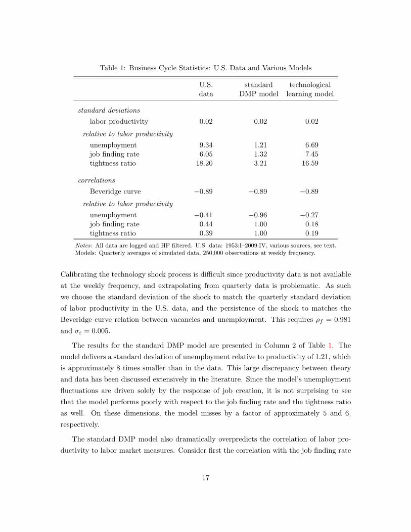
Table 1: Business Cycle Statistics: U.S. Data and Various Models
U.S. standard technologicaldata DMP model learning model
standard deviationslabor productivity 0.02 0.02 0.02
relative to labor productivityunemployment 9.34 1.21 6.69job finding rate 6.05 1.32 7.45tightness ratio 18.20 3.21 16.59
correlationsBeveridge curve −0.89 −0.89 −0.89
relative to labor productivityunemployment −0.41 −0.96 −0.27job finding rate 0.44 1.00 0.18tightness ratio 0.39 1.00 0.19
Notes: All data are logged and HP filtered. U.S. data: 1953:I–2009:IV, various sources, see text.Models: Quarterly averages of simulated data, 250,000 observations at weekly frequency.
Calibrating the technology shock process is difficult since productivity data is not available
at the weekly frequency, and extrapolating from quarterly data is problematic. As such
we choose the standard deviation of the shock to match the quarterly standard deviation
of labor productivity in the U.S. data, and the persistence of the shock to matches the
Beveridge curve relation between vacancies and unemployment. This requires ρf = 0.981
and σε = 0.005.
The results for the standard DMP model are presented in Column 2 of Table 1. The
model delivers a standard deviation of unemployment relative to productivity of 1.21, which
is approximately 8 times smaller than in the data. This large discrepancy between theory
and data has been discussed extensively in the literature. Since the model’s unemployment
fluctuations are driven solely by the response of job creation, it is not surprising to see
that the model performs poorly with respect to the job finding rate and the tightness ratio
as well. On these dimensions, the model misses by a factor of approximately 5 and 6,
respectively.
The standard DMP model also dramatically overpredicts the correlation of labor pro-
ductivity to labor market measures. Consider first the correlation with the job finding rate
17

and the tightness ratio. These are ‘jump’ variables in the model and the correlation with
productivity is perfect. In the data, these correlations are far from perfect. Unemployment
is a state variable in the model. As such, its correlation with productivity is smaller than
minus one, but still very close at −0.96. In the data, this correlation is only −0.41. For
Mortensen and Nagypal (2007), this evidence points to the importance of other driving
forces that are omitted from the standard analysis focusing solely on technology shocks. In
the next subsection, we illustrate how shocks to the technological learning rate represents
a potentially important omitted shock.
4.4 Technological Learning Rate Shocks
In this subsection, we document the cyclical properties of our benchmark model when
fluctuations are driven by shocks to the technological learning rate, λ. We model the
learning rate as following an AR(1) process:
λt = λ exp(xt), xt = ρλxt−1 + εt.
To maintain comparability with our analysis of technology shocks, we calibrate the volatility
of the shock to match the standard deviation of labor productivity observed in the data,
and the persistence to match the Beveridge curve. This implies a first-order persistence of
ρλ = 0.979 with a standard deviation of the shock innovation of σε = 0.161.
To be clear, we are interested in the quantitative evaluation of our benchmark model,
in so far as it illustrates the importance of the technological learning mechanism that we
study. But because of the model’s simplicity in featuring only two types of workers, its
predictions for cyclical fluctuations may be sensitive to a more detailed or ‘realistic’ setup.
In particular, in order to match age-earnings profiles, the productivity upgrade from type
L to H is large. Moreover, given that the average duration to realizing this upgrade is long,
shocks to the learning rate imply large swings in this duration over the business cycle. As
such, we consider a richer version of the model in the following subsection to demonstrate
robustness to having smaller upgrades and smaller fluctuations in the learning duration.
The results for the benchmark model are presented in Column 3 of Table 1. Learning
rate shocks generate substantial amplification in labor market variables. The volatility of
unemployment (relative to productivity) is more than 5 times that of the standard DMP
model (displayed in Column 2); the same is true regarding the volatility of the job finding
rate and the tightness ratio, relative to productivity.14
14These results are not due to the mechanisms stressed by Hagedorn and Manovskii (2008). We verify this
18

These results represent a marked improvement in terms of matching the U.S. data.
Fluctuations due to learning rate shocks account for 72% of the observed volatility of unem-
ployment. That the model does not capture all of its volatility is not surprising considering
that there is no role for cyclical variation in job separation. In terms of job creation, the
model’s amplification properties are clear. The model generates a volatility of the tightness
ratio relative to productivity, 16.59, that is very close to its observed volatility, 18.20. With
respect to the job finding rate, the model overpredicts its cyclical volatility relative to the
data. Hence, our model makes substantial progress toward resolving the unemployment
volatility puzzle, especially when viewed from the perspective of cyclicality in job creation.
Moreover, our model makes substantial progress toward resolving the unemployment-
productivity correlation puzzle. The model generates a correlation between these two vari-
ables of −0.27. This is close to the value of −0.41 observed in the data, and far from the
value near minus one generated by the standard DMP model driven by technology shocks.
This is mirrored in our model’s ability to generate realistic correlations of labor produc-
tivity with the job finding rate and the tightness ratio. In the data, these correlations are
0.44 and 0.39, respectively; in the model, they are 0.18 and 0.19. Learning rate shocks ef-
fectively decouple the dynamics of productivity from that of the labor market. This implies
business cycle behavior that is closer to that observed in the U.S. data, relative to models
where fluctuations are driven by shocks to technology.
4.5 Richer Heterogeneity
As discussed in subsection 4.4, the calibration of our benchmark, two type model implies
strong effects of fluctuations in the learning rate on job creation. Given this, we consider a
richer version of the model with N > 2 worker types. Each worker type faces a higher steady
state learning rate and a smaller productivity gain associated with any single upgrade,
relative to our benchmark model (with N = 2). In terms of notation, let fi denote the level
of output produced in a match between a firm and worker of type i, where i = 1, . . . , N .
For simplicity, we assume that a worker increases her productivity by one level at a time.
Let λi denote the probability, while matched, that a worker of type i upgrades to type i+1.
All other aspects of the model remain unchanged.
The characterization of the highest productivity, type N , market is identical to that of
by solving a version of our benchmark model (with N = 2) when driven solely by conventional technologyshocks. This version of the model features the same magnification result as in the standard DMP model.For brevity we do not present the results here, but they are available from the authors upon request.
19

the high productivity market summarized by the value functions, (5) through (8) (obviously,
with the H-subscripts replaced by N ’s). The value functions for all other workers and firms
with the potential for technological learning (types i = 1, . . . , N − 1) are given by:
Ui = z + βE[µ(θi)W ′i + (1− µ(θi))U ′i
], (12)
Wi = ωi + βE[λi[(1− δ)W ′i+1 + δU ′i+1
]+ (1− λi)
[(1− δ)W ′i + δU ′i
] ], (13)
Vi = −k + βE[q(θi)J ′i
], (14)
Ji = fi − ωi + βE[(1− δ)
[λiJ′i+1 + (1− λi)J ′i
] ]. (15)
To study the quantitative implications of this model extension, we pursue the same
calibration strategy as before. As such, we do not discuss the specification of the more
conventional model parameters, as this is done in the identical manner to subsection 4.1.
Here, we focus our discussion on the calibration of {fi, λi}Ni=1 and the process of ‘death and
rebirth’. For the sake of clarity and comparability, our strategy is to do this in as simple a
manner as possible.
As before, we set these parameters to match empirical age-earnings profiles. The average
worker takes approximately 25 years to achieve the maximal wage gains due to labor market
experience; during this time, earnings double. Given this, we choose N = 25 and set the
ratio of the lowest-to-highest productivity to be fN/f1 = 2. For simplicity, we follow
Ljungqvist and Sargent (1998) and specify all productivity levels to be equally spaced, so
that f1 = 0.5, f2 = 0.5208, . . ., fN−1 = 0.9792, and fN = 1. We restrict the steady state
learning rate between any two adjacent productivity levels to be symmetric; that is, λi = λ
for all i < N (and, obviously, λN = 0). Finally, we set λ = 0.0185, so that it takes the
average worker 54 weeks (or approximately one year) to realize a productivity upgrade;
in this way, it takes the average worker 25 years to progress from the lowest to highest
productivity level.
We choose φ, the constant probability of death, such that in the model’s steady state,
25% of workers are of type N with no further potential for upgrade. Finally, we must specify
how ‘dead’ workers are ‘reborn’ in order to maintain a constant unit mass of workers. For
symmetry, we do this so that in the model’s steady state, there is an equal measure of
workers of types 1 through N − 1 (specifically, 75%/24 = 3.13% of each type).15
15As a point of reference, we note that this is a close approximation to the observed age distribution of thelabor force. During the postwar period, the average fraction of labor force participants in 5-year age binsbetween the ages of 20-24 years and 45-49 years ranges from a low of 10.3% to a high of 12.5%; as discussedin Section 4, the average fraction over the age of 50 years is 25%.
20

Table 2: Business Cycle Statistics: U.S. Data and Technological Learning Model
U.S. benchmark N = 25data λ shocks λ shocks
standard deviationslabor productivity 0.02 0.02 0.02
relative to labor productivityunemployment 9.34 6.69 5.54job finding rate 6.05 7.45 6.18tightness ratio 18.20 16.59 13.80
correlationsBeveridge curve −0.89 −0.89 −0.89
relative to labor productivityunemployment −0.41 −0.27 −0.31job finding rate 0.44 0.18 0.22tightness ratio 0.39 0.19 0.22
Notes: All data are logged and HP filtered. U.S. data: 1953:I–2009:IV, various sources, see text.Models: quarterly averages of simulated data, 250,000 observations at weekly frequency.
The results are presented in Column 3 of Table 2. In columns 1 and 2, we display the
second moment statistics from Table 1 for the U.S. data and our benchmark model driven
by learning rate shocks, respectively. Overall, our results are remarkably robust when the
number of worker types is extended from N = 2 to N = 25. Again, the model displays
strong cyclical volatility. The standard deviation of HP-filtered unemployment is 5.54 times
that of labor productivity, which is not appreciably different from the value of 6.69 derived
from the benchmark model.16 Hence, the extended model still accounts for approximately
60% of the amplification observed in the data. In terms of job creation, the model fares
even better. Relative to productivity, the model generates a volatility of the job finding
rate that is very close to that in the data. Similar results are obtained for the tightness
ratio. We conclude that our model’s performance in terms of cyclical volatility is robust,
and importantly, makes progress in resolving the unemployment volatility puzzle.
Moreover, the results regarding cross correlations are robust. In the benchmark model,
the correlation between unemployment and productivity is −0.27. For the extended model,16In simulation experiments, we find that the model’s volatility of unemployment declines monotonically
as N increases from 2 to 25, but ‘flattens’ substantially for N > 10. For instance, between N = 10 andN = 25, the standard deviation of unemployment relative to productivity changes only from 5.62 to 5.54.
21

this is largely unchanged, at −0.31. Again, our model’s predicted correlation is not far
off relative to the U.S. data. The same is true regarding the correlations of productivity
with the job finding rate and the tightness ratio. The model generates realistic job creation
dynamics that are robust.
How large must the λ shocks be to account for the volatility of U.S. business cycles?
Our calibration strategy for the exogenous shock process is identical to before. This implies
a persistence of ρλ = 0.979 and a standard deviation of the innovation of σε = 0.185 for
our extended model. To quantify this volatility, note that the steady state learning rate
is calibrated so that the average employed worker realizes a productivity upgrade every
54 weeks. In the stochastic model, the 68% coverage region around the median learning
duration ranges from approximately 6 months to just over 2 years, due to business cycle
fluctuations. Given panel data evidence on the variation in the frequency of micro level
wage increases, we find our model’s volatility in learning rates to be very reasonable.
4.6 Understanding the Mechanism
To better understand the quantitative success of the model, we present impulse response
functions for unemployment and labor productivity in Figure 4.6. The vertical scale of both
panels is identical to facilitate comparison across models.
Panel A presents responses for the conventional business cycle impulse, specifically,
the response to a one standard deviation technology shock. Technology shocks have a
direct impact on matched workers’ productivity. Hence, labor productivity jumps upon
impact of the shock, gradually declining to steady state thereafter. This shock implies
an immediate impact on firm profit. From the free entry condition, vacancies respond
immediately. Because of the high empirical job finding rate that the model is calibrated to,
unemployment responds quickly, peaking 15 periods (or about 1 quarter) after the impact
period of the shock.
These responses clearly illustrate the shortcomings of technology shock-driven cycles in
the DMP model. Because the peak response of both unemployment and labor productivity
occur in the short-run, this implies a counterfactually strong correlation of the two variables
over the business cycle. Moreover, the response of unemployment is of the same order of
magnitude as that of productivity. Hence, as discussed extensively in the literature, the
model displays much weaker amplification of unemployment, relative to that observed in
the data.
22

Figure 1: Impulse Response Functions: Standard DMP and Technological Learning Models
0 50 100 150 20020
15
10
5
0
5
x 10 3 A: technology shock
0 50 100 150 20020
15
10
5
0
5
x 10 3 B: learning rate shock
Notes: Response to positive, one standard deviation shock. Solid (blue) line: unemploy-ment; dashed (red) line: labor productivity.
Panel B displays the response to a one standard deviation learning rate shock in our
extended (N = 25) models. In contrast to a technology shock, a learning rate shock has only
an indirect effect on labor productivity, via the type composition of the workforce. After a
positive shock to λ, the economy-wide upgrading rate rises. This causes productivity to rise
as workers shuffle from lower to higher types at a faster rate. But because the technological
learning process must still be undertaken, the dynamic response of productivity is persistent,
and only peaks about 110 periods (or 2 years) after the shock.
As a result, our model naturally decouples the dynamics between unemployment and
labor productivity. While unemployment peaks in the short-run (after 16 periods, or about
1 quarter after the shock), productivity peaks in the long-run. Hence, learning rate shocks
generate a low correlation between these two variables, as observed in the data.
Moreover, these shocks generate a substantially stronger effect on unemployment than
on productivity. To understand the response of unemployment, consider the benchmark
(N = 2) version, and the return to job creation, namely total surplus in type L matches,
displayed in equation (11). This surplus is determined largely by the value of learning,
∆, which represents the expected future profit gain from an upgrade. Since λ shocks
have a direct impact on the learning value, they have strong effects on job creation and
23

unemployment.
On the other hand, the effect of learning rate shocks on labor productivity is quantita-
tively weak. This can be seen analytically from the log-linearized response of productivity
to a λ shock. Given the model’s timing, there is no impact in the period of the shock, since
upgrading is reflected in output with a one period lag. The response of labor productivity
in the following period, LP t+1, is given by:
LP t+1 = X
{(nL + nHnH
)[λ(1− δ)
]λt −
(αθαLuLnL
)θLt
}.
Here, ni (ui) denotes the steady state measure of employed (unemployed) workers of type i,
θL is the steady state tightness ratio in market L, X is a constant (a function of parameters
and steady state values), and the circumflex represents log-linearized deviations from steady
state. The first term in the curly brackets indicates the effect of the λ shock. Its strength
depends on the steady state distribution of worker types, (nL + nH)/nH (the larger the
fraction of L types with the potential to upgrade, the bigger the effect), and importantly,
the level of the steady state learning rate, as captured by the term in square brackets.
In order to account for life-cycle earnings dynamics, our calibration requires a small value
for λ. Hence, the response of labor productivity to a learning rate shock is quantitatively
small.17
Finally, we note that the quantitative success of our model does not depend on the details
of the filtering procedure used. In particular, because the response of labor productivity is
smooth and persistent, it is possible that its cyclical fluctuations are subsumed into the HP-
filtered trend. In this case, our results may be overstating the volatility of unemployment
relative to productivity. To investigate this possibility, we derive second moment statistics
from our model and the U.S. data using a larger smoothing parameter in the HP filter.18
We increase it by a factor of 1000, from 105 (as in Shimer (2005a)) to 108. Increasing the
smoothing parameter makes the trend smoother, magnifying deviations from the trend. The
impact of this magnification is quantitatively larger for productivity than unemployment in
our model generated data. Using this smoothing parameter, the relative standard deviation
of unemployment to labor productivity in our benchmark (N = 2) model is 4.25, and 3.5917Deriving log-linearized expressions for labor productivity at longer time horizons is difficult, given the
need to track the dynamic response of the distribution of workers across types and employment status. Notealso that in the equation above, the second term in curly brackets is negative. This reflects the fact that apositive λ shock generates a response of job creation for L types (and no response in creation for H types).Hence, the distribution of employment shifts toward low productivity workers. This negative compositioneffect offsets the positive effect of faster upgrading on the response of labor productivity. However, in ournumerical experiments, this offsetting effect is small. See subsection 5.2 for further discussion.
18We thank Rob Shimer for suggesting this analysis to us.
24

in our extended (N = 25) model. The correlation between the two variables is −0.41
and −0.45, respectively. The corresponding values in the U.S. data are 5.53 and −0.24.
Hence, even with this extremely smooth filter, our model accounts for 65% − 77% of the
observed volatility of unemployment. Moreover, our model delivers a correlation between
unemployment and productivity similar to that found in the U.S. data.19
5 Further Analysis
In this section, we relate our model’s results to the recent “news shock” literature. Finally,
we embed our labor market framework into a general equilibrium business cycle model, to
further illustrate the robustness of our results.
5.1 Learning Rate Shocks and “News Shocks”
The decoupling of productivity and unemployment dynamics induced by shocks to the learn-
ing rate have important implications for our understanding of business cycle impulses. In
a recent paper, Beaudry and Portier (2006) use a number of structural VAR techniques to
identify shocks to productivity. They find that shocks to long-run productivity have essen-
tially no effect on productivity upon impact.20 Instead, productivity is found to respond in
a smooth, persistent manner. On the other hand, measures such as the stock market index
and employment are found to respond immediately (i.e., within the first quarter) to these
long-run TFP shocks.
Technological learning rate shocks generate dynamic responses that share these features.
Hence, shocks to the learning rate provide a theoretical interpretation of empirically identi-
fied “news shocks.” This is illustrated in Figure 2, where we plot impulse response functions
to a learning rate shock in our extended, N = 25 model of subsection 4.5. In Panel A, we
display the response of the model’s stock price index. We construct this index as a weighted
average of the present discounted value of firm profits in all match types, {Ji}Ni=1, where
the weights are the proportions of each type in the model’s steady state. A positive λ shock
causes the value of type i = 1, . . . , N − 1 matches to jump immediately as the ‘upside risk’19In comparison, applying this filter to the standard DMP model does not change its results: the relative
standard deviation of unemployment to productivity remains near one, and the correlation between thevariables remains near minus one.
20In their benchmark bivariate system, shocks identified to have a permanent impact on productivity arefound to have a small, negative effect on productivity upon impact (though the response is statistically indis-tinguishable from zero). And interestingly, shocks to stock market prices that are orthogonal to productivityupon impact generate a nearly identical dynamic response to TFP.
25

Figure 2: Impulse Response Functions to a Positive Learning Rate Shock
0 50 100 150 2000
0.01
0.02
0.03
A: stock price index
0 50 100 150 2000
0.005
0.01
0.015
0.02
0.025B: job finding rate
0 50 100 150 2000.02
0.015
0.01
0.005
0C: unemployment
0 50 100 150 2000
1
2
3
4 x 10 3 D: productivity
of these matches increases.21 Hence, the stock price index jumps upon impact of the shock;
the response gradually returns to zero as λ returns to its steady state value.
Panel B displays the response of the aggregate job finding rate. The learning rate shock
causes firm surplus for all type i < N firms to jump upon impact. From the free entry
condition, vacancies and job finding rates jump upon impact. Panel C displays the response
of the aggregate unemployment rate. Unemployment is a state variable, and therefore does
not respond in the period (i.e., week) of the shock. But because the model is calibrated
to a high aggregate job finding rate, as observed in the data, unemployment responds very
quickly after impact. Hence, economic activity, as measured by stock prices, job creation
and unemployment, respond within the quarter of the learning rate shock.
In contrast, labor productivity responds in a persistent, protracted manner. This is
evidenced in Panel D. Shocks to the learning rate induce gradual changes in the rate of
productivity upgrading. As a result, the productivity response is smooth, peaking ap-
proximately 120 periods—or over 2 years—after the initial shock. Hence, the productivity
response to learning rate shocks are observed in the long run. These features are consistent21Recall that the value of type N matches is unaffected.
26

Table 3: Business Cycle Statistics: U.S. Data and News Shock Model
U.S. standard 1 week 2 quartersdata model ahead model ahead model
relative standard deviationunemployment to productivity 9.34 1.21 1.22 1.32
correlationunemployment and productivity −0.41 −0.96 −0.97 −0.99
Notes: All data are logged and HP filtered. U.S. data: 1953:I–2009:IV, various sources, see text. Models:quarterly averages of simulated data, 250,000 observations at weekly frequency.
with the responses identified by Beaudry and Portier (2006).
Finally, we note that while our model conforms with the empirical evidence for new
shocks, the economic mechanism embodied by our learning rate shocks are distinct from
those in recent models. In those papers, news shocks are signals of technology shocks
that are to arrive a number of quarters in the future. Upon arrival, these innovations
immediately affect productivity. In contrast, shocks to the learning rate represent the arrival
of innovations that vary in their ease of implementation; their effects on labor productivity
are realized in a delayed manner, via the process of technological learning-by-doing.
This distinction is not simply a matter of interpretation: while learning rate shocks make
progress on rationalizing labor market dynamics in the DMP framework, conventionally
modeled news shocks do not. This is illustrated in Table 3, where news shocks are introduced
in the standard DMP model in the usual way—as the arrival of information at date 0 of a
change in productivity in period t.22 Column 2 presents results when t = 0, the timing for
the standard technology shock. Columns 3 and 4 present results for a one-week ahead (t = 1)
and two-quarter ahead (t = 26) news shock, respectively. As is obvious, the amplification
of unemployment volatility relative to productivity is essentially unchanged; the same is
true for the variables’ correlation. Both statistics are vastly different from that observed in
the U.S. data, as presented in Column 1. Hence, the manner in which “news shocks” are
modeled is important for rationalizing labor market dynamics in the DMP framework.22For brevity, we do not present details regarding this version of the model, and instead, make them
available upon request.
27

5.2 A Real Business Cycle Model
In this subsection, we embed our labor market framework into a general equilibrium, real
business cycle (RBC) model. The RBC model includes a number of features that are
absent from the DMP framework, most notably, diminishing marginal returns in produc-
tion, a wealth effect of business cycle shocks on labor market outcomes, and a consump-
tion/investment choice. The primary purpose of this analysis is to show robustness of the
cyclical properties of unemployment to the inclusion of these neoclassical features. A sec-
ondary purpose is to ensure that our model maintains the success of the standard RBC
model regarding the cyclical behavior of consumption, investment, and output.
5.2.1 Description
Our model is a simplified version of Andolfatto (1996), modified to include technological
learning as in Section 2. As such, we keep our exposition brief. The economy is populated
by a representative household who provides consumption insurance to all of its members (a
continuum of individuals with measure one). Each individual member derives utility from
consumption, and incurs a utility cost of working denoted γ. Let nL and nH denote the
measures of employed type L and type H individuals, and uL and uH denote the measures
of unemployed individuals.
Let c denote consumption, and k denote capital. The household’s budget constraint is
given by:
c+ k′ = (1− d+ r)k + ωLnL + ωHnH + b(uL + uH) + π. (16)
Here r is the rental rate on capital, d is its depreciation rate, and b is an unemployment
benefit; π represents profits earned by firms (and distributed to the household) minus lump-
sum taxes paid to the government. The government maintains a balanced budget, and levies
taxes to cover unemployment benefits. Let V denote the value function of the household,
specifically:
V(k, nL, nH , uL, uH) ≡ maxc,k′
{ln c− γ(nL + nH) + βEV(k′, n′L, n
′H , u
′L, u
′H)},
subject to constraint (16) and the following laws of motion:
n′L = (1− δ)(1− λ)nL + µ(θL)uL,
n′H = (1− δ)nH + (1− δ)λnL + µ(θH)uH ,
u′L = δ(1− λ)nL + (1− µ(θL))uL,
u′H = δnH + δλnL + (1− µ(θH))uH .
28

The representative firm has access to two ‘production lines’: one operated by type L
workers, the other by type H workers. Both production lines use capital and labor as
inputs in a Cobb-Douglas production function to produce a homogenous final good. This
final good serves either as consumption or investment. As will be discussed shortly, the
assumption of two production lines facilitates comparison to our previous DMP model.
The firm faces a dynamic problem, with state variables consisting of the stock of current
employment, nL and nH . In each period, it chooses the number of vacancies to maintain,
and the amount of capital to rent. The value of the firm, J , is defined as:
J (nL, nH) ≡ maxvL,vH ,kL,kH
{ALk
aLn
1−aL +AHk
aHn
1−aH − r(kL + kH)
− ωLnL − ωHnH − κ(vL + vH) + E[QJ (n′L, n
′H)] },
subject to
n′L = (1− δ)(1− λ)nL + q(θL)vL,
n′H = (1− δ)nH + (1− δ)λnL + q(θH)vH .
Here, a is the capital share of income, and Q is the stochastic discount factor (which, in
equilibrium, equals the household’s intertemporal marginal rate of substitution). In posting
vacancies, the firm takes the job filling probabilities as given.
The first order conditions with respect to capital deliver the following no arbitrage
condition:
r = aAL (nL/kL)1−a = aAH (nH/kH)1−a . (17)
The first order conditions with respect to vacancies deliver the usual free entry conditions:
κ = q(θL)E[QJn′L
],
κ = q(θH)E[QJn′H
],
where the value of the marginal worker is given by:
JnL = MPnL − ωL + (1− δ){
(1− λ)E[QJn′L
]+ λE
[QJn′H
]},
JnH = MPnH − ωH + (1− δ)E[QJn′H
],
and MPnL = (1− a)AL(kL/nL)a, MPnH = (1− a)AH(kH/nH)a.
As before, we assume that worker compensations are the result of generalized Nash
bargaining between the firm and worker. It can be shown that these are given by the
29

following expressions:
ωL = τMPnL + (1− τ)(b+ γc) + τκθL − βλE[U ′]c,
ωH = τMPnH + (1− τ)(b+ γc) + τκθH , (18)
where
U =1cτκ[θH − θL] + βE[U ′].
Finally, feasibility requires that
c+ k′ + κ(vL + vH) = ALkaLn
1−aL +AHk
aHn
1−aH + (1− d)k,
where kL + kH = k.
5.2.2 Analysis
We first discuss a number of the RBC model features, before proceeding to the numerical
analysis. In the standard DMP model, match output is given parametrically. Hence, the
output of an additional type L worker is always fL; the marginal product of a type H
worker is always fH . In contrast, the Cobb-Douglas production function in this model
features diminishing marginal product of labor. This implies that as employment rises, all
else equal, labor productivity falls.
Despite diminishing marginal product of labor, our assumption of two production lines
ensures that the productivity upgrade for an individual worker is constant. From the
definitions of MPnL and MPnH , and the no arbitrage condition, (17):
MPnHMPnL
=(AHAL
) 11−a
.
This facilitates comparison with our benchmark model, where the productivity upgrade is
given parametrically by fH/fL.
Finally, we note that the current model features a wealth effect on the labor market that
is not present in the DMP framework. Equilibrium in the labor market can be summarized
as the intersection between the ‘job creation’ curve and the ‘wage’ curve in ω–θ space; these
stand in for labor demand and labor supply curves, respectively. In the standard DMP
model, the wage curve is simply ω = τf + (1− τ)z+ τkθ. The flow value of unemployment,
z, is constant over the cycle. This is not the case in the RBC version. This can be seen
most easily for the H market, where the wage curve is equation (18). The flow value of
unemployment, (b+ γc), varies with current consumption.
30

Table 4: Business Cycle Statistics: U.S. Data and and Various RBC Models
U.S. standard technologicaldata DMP version learning version
relative standard deviationunemployment to productivity 9.34 1.03 6.42
correlationunemployment and productivity −0.41 −0.97 −0.03
std devs relative to outputemployment 0.56 0.06 0.35consumption 0.85 0.43 0.60investment 3.91 3.86 2.88
correlations with outputemployment 0.78 0.97 0.38consumption 0.88 0.71 0.92investment 0.90 0.96 0.94
Notes: All data are logged and HP filtered. U.S. data: 1953:I–2009:IV, various sources, see text. Models:quarterly averages of simulated data, 250,000 observations at weekly frequency.
An expansionary shock generates a standard ‘shift out’ of the job creation curve in both
the standard DMP model and the RBC version. But in the RBC model, the positive wealth
effect of the shock generates a rise in consumption. This causes a ‘shift back’ of the wage
curve that is absent from the standard DMP model. Hence, the wealth effect mitigates the
equilibrium response of job creation and unemployment.
Having established the qualitative implications of the neoclassical framework, we turn
to quantifying their importance for the cyclical behavior of unemployment and productivity.
Our calibration strategy is identical to that described in subsection 4.1. For brevity, we
discuss only the specification of the new parameters.23 The capital share of income is set
to a = 0.3. Given this, we set AL and AH so that MPnH/MPnL = 2, as in our previous
analysis. The capital depreciation rate is set to d = 0.002 (at the weekly frequency), to
match a steady state investment to output ratio of 0.2.
In Table 4, we present the key business cycle statistics for our model driven by learning
rate shocks; this is in Column 3. Columns 1 and 2 present the same statistics for the23Further details are available from the authors upon request.
31
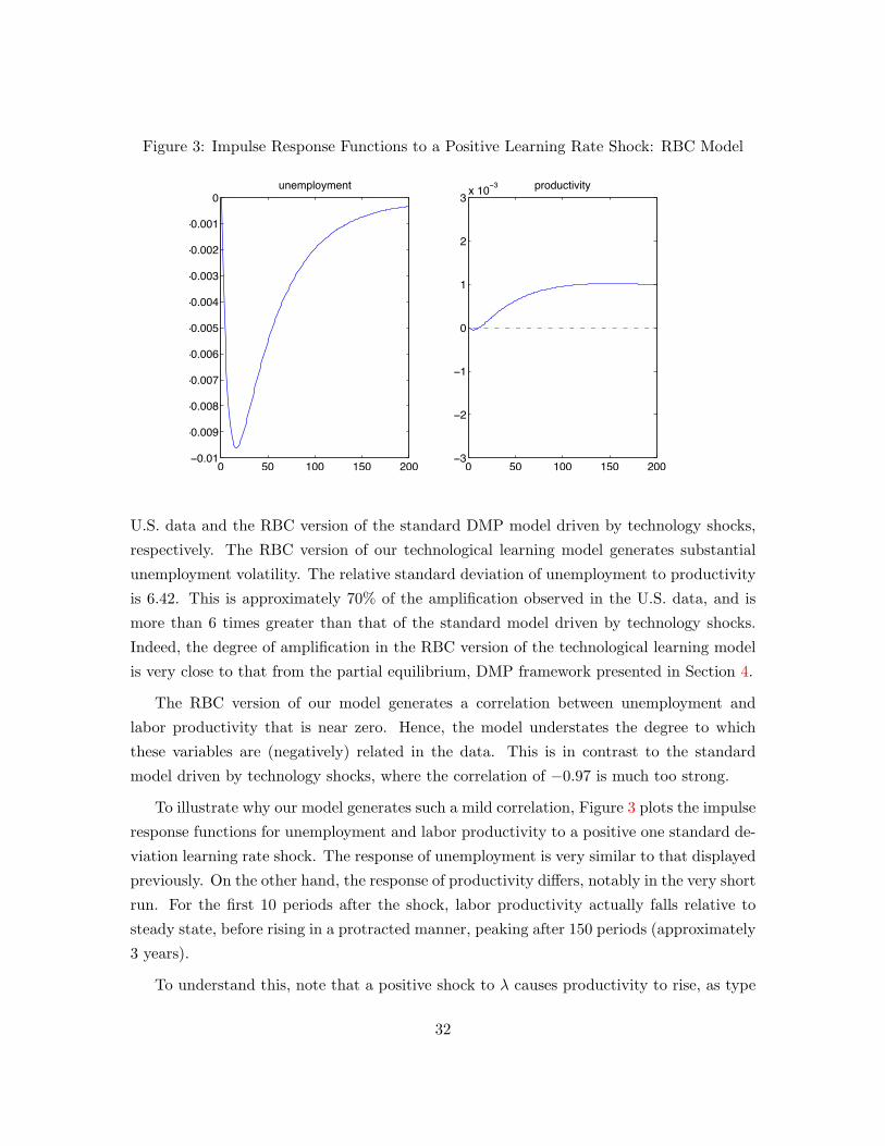
Figure 3: Impulse Response Functions to a Positive Learning Rate Shock: RBC Model
0 50 100 150 2000.01
0.009
0.008
0.007
0.006
0.005
0.004
0.003
0.002
0.001
0unemployment
0 50 100 150 2003
2
1
0
1
2
3 x 10 3 productivity
U.S. data and the RBC version of the standard DMP model driven by technology shocks,
respectively. The RBC version of our technological learning model generates substantial
unemployment volatility. The relative standard deviation of unemployment to productivity
is 6.42. This is approximately 70% of the amplification observed in the U.S. data, and is
more than 6 times greater than that of the standard model driven by technology shocks.
Indeed, the degree of amplification in the RBC version of the technological learning model
is very close to that from the partial equilibrium, DMP framework presented in Section 4.
The RBC version of our model generates a correlation between unemployment and
labor productivity that is near zero. Hence, the model understates the degree to which
these variables are (negatively) related in the data. This is in contrast to the standard
model driven by technology shocks, where the correlation of −0.97 is much too strong.
To illustrate why our model generates such a mild correlation, Figure 3 plots the impulse
response functions for unemployment and labor productivity to a positive one standard de-
viation learning rate shock. The response of unemployment is very similar to that displayed
previously. On the other hand, the response of productivity differs, notably in the very short
run. For the first 10 periods after the shock, labor productivity actually falls relative to
steady state, before rising in a protracted manner, peaking after 150 periods (approximately
3 years).
To understand this, note that a positive shock to λ causes productivity to rise, as type
32

L workers upgrade to type H at a faster rate. This is offset by two factors in the short-run.
First, the shock generates job creation in the L market (where technological learning is
relevant). This creates a negative composition effect, as the distribution of employment
shifts toward type L workers. In addition, employment is subject to diminishing marginal
returns: as more type L workers are hired, their average productivity is dragged down
(an effect that is absent from the standard DMP framework). These two countervailing
effects dominate the positive effect of the λ shock on productivity in the short run, and
are responsible for the very mild correlation between productivity and unemployment. Of
course, one could easily introduce mechanisms that are common in RBC analysis, to mitigate
these countervailing effects (for example, cyclical capital utilization). However, given the
primary emphasis of this exercise, this is beyond the scope of this paper.
Finally, the technological learning model does a good job on the dimensions typically
studied in RBC models, namely the cyclical behavior of output, consumption, investment,
and employment. Our model’s predictions regarding the relative volatility of consumption
and investment to output are on par with those from the standard RBC model driven by
technology shocks. And not surprisingly, our model greatly outperforms the standard model
with respect to the relative volatility of employment.
Finally, we note that learning rate shocks generate business cycle comovement: output,
employment, consumption and investment all move together. Hence, our model generates
realistic business cycle dynamics. Moreover, our model delivers comovement while simulta-
neously generating impulse responses resembling those of empirically identified news shocks.
This last task has proven problematic in standard RBC models driven by anticipated tech-
nology shocks. A comprehensive analysis of the RBC version of our model with respect to
the new shock literature would require extending the model in a number of directions (for
instance, including an ‘intensive margin’ of labor effort). This is beyond the scope of this
paper, and we leave this to ongoing and future work.
6 Conclusion
In this paper, we have focused on two key labor market observations in postwar U.S. data.
The first is that unemployment is very volatile over the business cycle relative to labor
productivity. The second is that cyclical fluctuations in unemployment and productivity
are only mildly negatively correlated. The canonical model of equilibrium unemployment,
when driven by technology shocks, fails to account for either of these facts.
33

We propose a model of technological learning that makes progress on both shortcomings.
Specifically, we construct a tractable search-and-matching model in which: (a) it takes
time for workers to become fully productive with new technology, and (b) shocks to the
speed or ease of learning are a source of business cycle fluctuations. Quantitative analysis
indicates that our model accounts for 60%− 70% of the relative volatility of unemployment
to productivity, and essentially all of the relative volatility of job finding rates, observed
in the U.S. data. Moreover, our model delivers a correlation between unemployment and
labor productivity that is very close to the data.
34

A Data Sources
Our measure of unemployment is the quarterly average of the seasonally adjusted monthlyseries constructed by the Bureau of Labor Statistics (BLS) from the Current PopulationSurvey (CPS). Our measure of labor productivity is (quarterly, seasonally adjusted) outputdivided by employment in the nonfarm business sector as constructed by the BLS MajorSector Productivity program. To construct the job finding rate, we follow the approachof Shimer (2005a,b, 2007), using monthly data on employment, unemployment, and short-term unemployment tabulated from the CPS. We use vacancy data provided by Barnichon(2010), divided by unemployment, to construct the tightness ratio. Specifically, we use his“composite Help-Wanted Index” which combines information on the number of newspaperand online job advertisements compiled by the Conference Board.
Quarterly data on aggregate output and its expenditure components are obtained fromthe National Income and Product Accounts. Specifically, real output, consumption, andinvestment refer to seasonally adjusted gross domestic product, personal consumption ex-penditures, and gross private domestic investment, respectively, expressed in chained 2005dollars. Finally, employment refers to the quarterly average of the seasonally adjustedmonthly series for the civilian employment-population ratio, constructed by the BLS fromCPS data.
B Efficiency
To show that our equilibrium is efficient, we derive equations that fully characterize thesolution to a planner’s problem and show that the same equations characterize equilibriumunder Hosios (1990)’s condition.
B.1 Compensations
To begin, we derive the compensations from generalized Nash bargaining. These are re-quired for the characterizations below. The market for high productivity workers is identicalto that of the standard DMP model. Therefore, the compensation in such matches is entirelystandard:
ωH = τ(fH + κθH) + (1− τ)z. (19)
To obtain the compensation in low productivity matches, begin with proportionality ofsurplus:
(1− τ) (WL − UL) = τJL.
Worker surplus can be expressed as:
(WL − UL) = ωL − z + βE{
(1− δ)[λ(W ′H − U ′H
)+ (1− λ)
(W ′L − U ′L
) ]− µ(θL)
(W ′L − U ′L
)+ λ
(U ′H − U ′L
)},
35

or:
(1− τ) (WL − UL) = (1− τ)(ωL − z) + βE{
(1− δ)τ [λJ ′H + (1− λ)J ′L]
− τµ(θL)J ′L + (1− τ)λ(U ′H − U ′L
)}.
Equating this with τJL and using free entry, we get:
ωL = τ(fL + κθL) + (1− τ)z − (1− τ)λβE[U ′H − U ′L
]. (20)
The last term is (1− τ) times the worker’s value of learning.
The worker’s value of learning can be simplified by noting that:
UH − UL = βE[µ(θH)
(W ′H − U ′H
)− µ(θL)
(W ′L − U ′L
)+ [U ′H − U ′L]
].
Using the proportionality of surplus and the free entry condition again, we get:
UH − UL = τκ(θH − θL) + βE[U ′H − U ′L]
= τκE∞∑s=0
βs(θ+sH − θ
+sL ) (21)
where τ = τ/(1− τ), θ+0i = θi, θ+1
i = θ′i, θ+2i = θ′′i , and so on.
B.2 A Planner’s Problem
Let V (uL, uH , nL, nH) denote the value function of the planner who inherits unemploymentui for type i ∈ {L,H} and employment ni for type i ∈ {L,H}:
V (uL, uH , nL, nH) = max{θi,u′i,n′i}i={L,H}
{(uL + uH)z + nLfL + nHfH
− κ(uLθL + uHθH) + βV (u′L, u′H , n
′L, n
′H)},
subject to the following laws of motion:
u′L ≥ (1− µ(θL))uL + (1− λ)δnL,u′H ≥ (1− µ(θH))uH + λδnL + δnH ,
n′L ≤ µ(θL)uL + (1− λ)(1− δ)nL,n′H ≤ (1− δ)nH + µ(θH)uH + λ(1− δ)nL.
Setting uL + uH + nL + nH = 1 and letting λui be the multiplier on the law of motionfor ui and λni be the multiplier on the law of motion for ni, the first-order conditions withrespect to θi, i ∈ {L,H}, are:
−κ+ µ′(θL)(λuL + λnL) = 0,
36

−κ+ µ′(θH)(λuH + λnH ) = 0.
The first order conditions with respect to u′i and n′i, i ∈ {L,H}, are:
βVui(u′L, u
′H , n
′L, n
′H) + λui = 0,
βVni(u′L, u
′H , n
′L, n
′H)− λni = 0.
Finally, the envelope conditions are:
VuL = z − κθL − λuL(1− µ(θL)) + λnLµ(θL),VuH = z − κθH − λuH (1− µ(θH)) + λnHµ(θH),VnL = fL − λuL(1− λ)δ − λuHλδ + λnL(1− λ)(1− δ) + λnHλ(1− δ),VnH = fH − λuHδ + λnH (1− δ).
Combining the first-order and envelope conditions, the following equations characterizea steady state:
λuL + λnL =κ
µ′(θL)(22)
λuH + λnH =κ
µ′(θH)(23)
β(z − κθL + µ(θL)(λuL + λnL)− λuL
)+ λuL = 0 (24)
β(z − κθH + µ(θH)(λuH + λnH )− λuH
)+ λuH = 0 (25)
β(fL − δ
[(1− λ)(λuL + λnL) + λ(λuH + λnH )
]+ (1− λ)λnL + λλnH
)− λnL = 0 (26)
β(fH − δ(λuH + λnH ) + λnH
)− λnH = 0 (27)
It will prove convenient to use these equations get expressions for some of the multipliers.From equation (24), we have:
λuL = −β(αz + (1− α)θLκ)α(1− β)
. (28)
Similarly, from equation (25), we have:
λuH = −β(αz + (1− α)θHκ)α(1− β)
, (29)
and from equation (27) we have:
λnH =β(αfH − δθHκ/µ(θH))
α(1− β). (30)
37

B.2.1 Market H
Notice that equations (23), (29) and (30) fully characterize θH in an unrelated way to θL,or submarket L in general. Using (29) and (30) in (23):
β(αfH − δθHκ/µ(θH)− αz − (1− α)θHκ
)α(1− β)
=κ
µ′(θH).
Using the fact that µ′(θ) = αµ(θ)/θ, we have:
β
(α(fH − z)− (1− α)θHκ− δ
θHκ
µ(θH)
)=
(1− β)αθHκαµ(θH)
.
Rearranging, θH is characterized by:
β(α(fH − z)− (1− α)θHκ
)1− β(1− δ)
=θHκ
µ(θH). (31)
B.2.2 Market L
Rewrite equation (26) as follows:
λnL = β(fL − δ(1− λ)(λuL + λnL)− δλ(λuH + λnH )− λ(λnL − λnH )),
where β = β/(1− β). We now need an expression for λnL − λnH . From equations (22) and(23), we have
λnL − λnH =κ
µ′(θL)− κ
µ′(θH)+ λuH − λuL .
Using the expressions for λuH and λuL from equations (28) and (29), this is
λnL − λnH =κ
µ′(θL)− κ
µ′(θH)+ (β/α)(1− α)(θL − θH)κ.
So λnL becomes
λnL = β[fL − δ(1− λ)(λuL + λnL)− δλ(λuH + λnH )
− λ(
κ
µ′(θL)− κ
µ′(θH)+ (β/α)(1− α)(θL − θH)κ
)],
or, rearranging,
λnL = β
[fL − [δ(1− λ) + λ]
κ
µ′(θL)+ (1− δ)λ κ
µ′(θH)− λ(β/α)(1− α)(θL − θH)κ
].
Using this last equation together with the expression for λuL from equation (28) in equa-tion (22), we have
β[fL − z − (1− α)θLκ/α− [δ(1− λ) + λ]
κ
µ′(θL)+ (1− δ)λ κ
µ′(θH)
− λ(β/α)(1− α)(θL − θH)κ]
=κ
µ′(θL).
38

Grouping terms and rearranging,
β
[fL − z − (1− α)θLκ/α+ (1− δ)λ κ
µ′(θH)+ λ(β/α)(1− α)(θH − θL)κ
]=
κ
µ′(θL), (32)
where β = β/(1− β(1− δ)(1− λ)). Given the value of θH which solves equation (31), thislast expression characterizes θL.
B.3 Relation to Equilibrium
B.3.1 Market H
The steady state value of the firm in market H is
JH =fH − ωH
1− β(1− δ).
Using the wage equation (19) in the free-entry condition βµ(θH)JH = θHκ, we have
β((1− τ)(fH − z)− τθHκ
)1− β(1− δ)
=θHκ
µ(θH).
Clearly, this is equivalent to its counterpart (31) from the Planner’s problem if τ = 1− α.
B.3.2 Market L
The free entry condition in that market reads
βµ(θL)JL = θLκ,
whereJL = fL − ωL + β(1− δ)[λJH + (1− λ)JL].
We can use the free entry condition JH = θHκ/βµ(θH) to get
JL =fL − ωL + β(1− δ)λθHκ/βµ(θH)
1− β(1− δ)(1− λ).
From equations (20) and (21), the wage in market L can be written as
ωL = τ(fL + κθL) + (1− τ)z − βλτκ(θH − θL).
Using this wage in JL, the free entry condition becomes
βµ(θL)fL −
(τ(fL + κθL) + (1− τ)z − βλτκ(θH − θL)
)+ (1− δ)λθHκ/µ(θH)
1− β(1− δ)(1− λ)= θLκ.
39

Rearranging, we have
β[(1− τ)(fL − z)− τκθL + βλτκ(θH − θL) + (1− δ)λακ/µ′(θH)
]= ακ/µ′(θL). (33)
If α = 1− τ , this becomes
β[fL − z − (1− α)θLκ/α+ (1− δ)λκ/µ′(θH) + λ(β/α)(1− α)κ(θH − θL)
]= κ/µ′(θL),
which is identical to its counterpart (32) from the Planner’s problem.
C Directed Search
Given the previous result regarding efficiency, it is perhaps not surprising that the equi-librium of our model is robust to the decentralization and determination of wages. Inparticular, it is robust to the following “wage posting” setup.
To proceed, we maintain the assumption that the labor market is segmented by workertype; that is, a type L worker cannot search for a vacancy posted for a type H worker,and vice versa. The interpretation is as follows. In the market for type H, firms post awage that they commit to pay upon matching with a worker in each period that they areproductive. A firm who meets with a type H worker is certain of the match output untilexogenous separation. This allows a firm to post a single wage. As will become obvious, thisimplies that competitive search equilibrium in this market is identical to that in a standardDMP model.
In the type L market, firms post wages to attract unemployed workers where matchesface a probability of upgrading to a type H match. Therefore, a firm posts a wage, ωL, thatit commits to while the match produces output fL, and must also post a wage commitmentin the event that the match upgrades. For simplicity, assume that firms commit to pay the(unique) equilibrium wage that is being posted by firms in the type H market.
Workers observe all posted wages and choose which wage submarket to search in (withinthe type market). Both workers and firms observe the market tightness, and hence, the jobfinding and filling rates implied by their choice. Given this setup, it suffices to show thatthe tightness ratios in each market are unique, and that the wages posted in each marketare identical to the Nash bargained wages from our model.
C.1 H Market
For simplicity, we focus on deterministic steady state in our model. Using equation (6), thevalue function for a type H unemployed worker can be rearranged as:
(1− β)UH = z + βµ(θH)[ωH − (1− β)UH ], (34)
where β = β/(1 − β(1 − δ)). Given that the worker is directing her search, she choosesthe wage submarket that offers her the highest UH . For a given level of UH , (34) gives the
40

indifference trade-off between wage and tightness: the worker can be compensated for alower ωH through an appropriately higher job finding rate, µ(θH).
From equations (7) and (8), we obtain the value of maintaining a type H vacancy insteady state:
VH = −κ+ βq(θH)(fH − ωH). (35)
The firm’s problem is to choose the (θH , ωH) pair that maximizes VH . Let UH denote thehighest utility a type H worker can attain by applying to some firm’s vacancy. The profitmaximizing firm knows that in order for any workers to search for its vacancy, its (θH , ωH)must provide at least as much utility as UH . Hence, the firm maximizes VH subject to theconstraint (34).
At this point it is useful to consider a change of variable for the sake of algebra. Letυ = θ−1. Previewing our choice in Section 4, assume a Cobb-Douglas matching function,and define:
µ(υ) = υ−α = θα = µ(θ),
q(υ) = υ1−α = θα−1 = q(θ).
Note that q(υ) = υµ(υ).
Subbing (34) into (35) and using the change of variable, we obtain the following as thefirm’s problem:
maxυH
{− κ+ βυH µ(υH)fH − υH
[(1− β)UH
(1 + βµ(υH)
)− z]}. (36)
The FONC can be written as:
β[µ(υH) + υH µ
′(υH)][fH − (1− β)UH
]= (1− β)UH − z. (37)
Given the Cobb-Douglas functional form, µ(υH)+υH µ′(υH) = (1−α)µ(υH) = (1−α)µ(θH).Since the firm takes the level of UH as given, and since µ(θH) is monotone increasing, thereis a unique θH that satisfies (37); all firms post the same wage, implying the same markettightness.
To find the posted wage, rearrange (37) as:
(1− β)UH[1 + (1− α)βµ(θH)
]= (1− α)βµ(θH)fH + z.
Subing this into (34) for (1− β)UH , and using the free entry condition, obtains:
ωH = (1− α)fH + (1− α)θHκ+ αz.
Hence, the steady-state per period wage with wage posting and directed search is identicalto the case with Nash bargaining, when τ = 1− α.
41

C.2 L Market
Proceeding as above, the value of a type L unemployed worker can be expressed as:
(1− β)UL = z + βµ(θL)[ωL + βλ
[(1− δ)(WH − UH) + (UH − UL)
]− (1− β)UL
],
where β = β/(1− β(1− δ)(1− λ)). Using the change of variable and rearranging we get:
βµ(υL)ωL =[1 + βµ(υL)
](1−β)UL− z− βµ(υL)βλ[(1− δ)(WH −UH) + (UH −UL)]. (38)
The value function for a type L vacancy is:
VL = −κ+ βq(θL)[fL − ωL + βλ(1− δ)JH ]. (39)
Making the change of variable and subbing in from above we get:
maxυL
{− κ+ βυLµ(υL)
[fL + βλ(1− δ)JH
]− υL
[(1− β)UL
(1 + βµ(υL)
)− z − βµ(υL)βλ
[(1− δ)(WH − UH) + (UH − UL)
]]}. (40)
After rearranging, the FONC is:[1 + (1− α)βµ(υL)
](1− β)UL = (1− α)βµ(υL)
[fL + βλ(1− δ)(JH +WH − UH)
+ βλ(UH − UL)]
+ z.
Given that the firm takes JH ,WH , UH and UL as given, this establishes that θL is unique.
Subbing this into (38) and rearranging obtains:
ωL + αβλ(1− δ)(WH − UH) + αβλ(UH − UL) = αz + (1− α)fL+ (1− α)βλ(1− δ)JH + (1− α)βµ(θL)
[fL − ωL + βλ(1− δ)JH
].
Using the free entry condition this simplifies to:
ωL = (1− α)fL + (1− α)θLκ+ αz − αβλ(UH − UL) + βλ(1− δ)[(1− α)JH − α(WH − UH)].
Given that (1− α)JH = α(WH − UH), the last term cancels out. Hence, the expression forωL is the exact expression obtained with Nash bargaining, when τ = 1− α.
D Proof of Proposition 2
We begin by establishing a lemma.
Lemma 2 With respect to log-linear deviations from steady state in response to a λ shock,(θL, UL, TSL,∆) comove positively.
42

Proof. Using the free entry condition, equation (10), and assuming a Cobb-Douglas match-ing function so that q(θ) = θα−1, we obtain the log-linearized relationship:
T SL = (1− α)θL.
From the expression for the value of unemployment, equation (1), in steady state:
UL =[
τκθL(1− β)UL
]θL.
From the definition of total surplus, equation (11):
∆ =[TSL[1− β(1− δ)](1− α) + θLτκ
∆
]θL.
Given this lemma, proving Proposition 2 requires showing that θL responds positivelyto a λ shock.
Proof. Since ∆ = λβ [(1− δ)(TSH − TSL) + (UH − UL)], log-linearizing we obtain:
∆∆ = ∆λ− λβ[(1− δ)TSLT SL + ULUL
].
This uses the fact that T SH = UH = 0 in response to λ. Using the derivations fromLemma 2:
[1− β(1− δ)](1− α)TSLθL + τκθLθL = ∆λ− λβ[(1− δ)TSLT SL + ULUL
],
[1− β(1− δ)](1− α)TSLθL + τκθLθL = ∆λ− λβ(1− δ)(1− α)TSLθL −λβ
1− βτκθLθL.
Therefore:
∆λ ={
[1− β(1− δ)(1− λ)] (1− α)TSL +[1 +
λβ
1− β
]τκθL
}θL.
Since both ∆ and the term in curly brackets are positive, this implies that θL comovespositively with a λ shock.
43

References
Andolfatto, D. (1996). Business cycles and labor-market search. American Economic Re-
view 86 (1), 112–132.
Argote, L. and D. Epple (1990). Learning curves in manufacturing. Science 247, 920–924.
Balasubramanian, N. and M. Lieberman (2010). Industry learning environments and the
heterogeneity of firm performance. Strategic Management Journal 31, 390–412.
Barnichon, R. (2010). Building a composite help-wanted index. Economics Letters 109 (3),
175–178.
Beaudry, P. and B. Lucke (2010). Letting different views about business cycles compete. In
D. Acemoglu, K. Rogoff, and M. Woodford (Eds.), NBER Macroeconomics Annual 2009,
Volume 24. University of Chicago Press.
Beaudry, P. and F. Portier (2006). Stock prices, news and economic fluctuations. American
Economic Review 96 (4), 1293–1307.
Beaudry, P. and F. Portier (2007). When can changes in expectations cause business cycle
fluctuations in neo-classical settings? Journal of Economic Theory 135 (1), 458–477.
Benhabib, J., R. Rogerson, and R. Wright (1991). Homework in macroeconomics: House-
hold production and aggregate fluctuations. Journal of Political Economy 99 (6), 1166–
1187.
Bruemann, B. (2008). What elasticity of the matching function is consistent with us aggre-
gate labor market data? Unpublished manuscript.
Brugemann, B. and G. Moscarini (2010). Rent rigidity, asymmetric information, and volatil-
ity bounds in labor markets. Review of Economic Dynamics 13 (3), 575–596.
Christiano, L. J. and M. Eichenbaum (1992). Current real-business-cycle theories and
aggregate labor-market fluctuations. American Economic Review 82 (3), 430–450.
Comin, D. A., M. Gertler, and A. M. Santacreu (2009). Technology innovation and diffusion
as sources of output and asset price fluctuations. Working Paper 15029, National Bureau
of Economic Research.
Costain, J. S. and M. Reiter (2008). Business cycles, unemployment insurance, and the
calibration of matching models. Journal of Economic Dynamics and Control 32 (4),
1120–1155.
44

den Haan, W. J. and G. Kaltenbrunner (2009). Anticipated growth and business cycles in
matching models. Journal of Monetary Economics 56 (3), 309–327.
Diamond, P. A. (1982). Aggregate demand management in search equilibrium. Journal of
Political Economy 90 (5), 881–894.
Elsby, M. W. L., R. Michaels, and G. Solon (2009). The ins and outs of cyclical unemploy-
ment. American Economic Journal: Macroeconomics 1 (1), 84–110.
Fujita, S. and G. Ramey (2009). The cyclicality of separation and job finding rates. Inter-
national Economic Review 50 (2), 415–430.
Gertler, M. and A. Trigari (2009). Unemployment fluctuations with staggered Nash wage
bargaining. Journal of Political Economy 117 (1), 38–86.
Hagedorn, M. and I. Manovskii (2008). The cyclical behavior of equilibrium unemployment
and vacancies revisited. American Economic Review 98 (4), 1692–1706.
Hagedorn, M. and I. Manovskii (2010). Productivity and the labor market: Co-movement
over the business cycle. International Economic Review Forthcoming.
Hall, R. E. (2005). Employment fluctuations with equilibrium wage stickiness. American
Economic Review 95 (1), 50–65.
Hall, R. E. and P. R. Milgrom (2008). The limited influence of unemployment on the wage
bargain. American Economic Review 98 (4), 1653–1674.
Hornstein, A., P. Krusell, and G. L. Violante (2005). Unemployment and vacancy fluc-
tuations in the matching model: Inspecting the mechanism. Federal Reserve Bank of
Richmond Economic Quarterly 91 (3), 19–51.
Hosios, A. J. (1990). On the efficiency of matching and related models of search and
unemployment. Review of Economic Studies 57 (2), 279–298.
Irwin, D. A. and P. J. Klenow (1994). Learning-by-doing spillovers in the semiconductor
industry. Journal of Political Economy 102 (6), 1200–1227.
Jaimovich, N. and S. Rebelo (2009). Can news about the future drive the business cycle?
American Economic Review 99 (4), 1097–1118.
Ljungqvist, L. and T. J. Sargent (1998). The European unemployment dilemma. Journal
of Political Economy 106 (3), 514–550.
45

Ljungqvist, L. and T. J. Sargent (2004). European unemployment and turbulence revisited
in a matching model. Journal of the European Economic Association 2 (2–3), 456–467.
Menzio, G. and S. Shi (2011). Efficient search on the job and the business cycle. Unpublished
manuscript.
Merz, M. (1995). Search in the labor market and the real business cycle. Journal of
Monetary Economics 36 (2), 269–300.
Mortensen, D. T. (1982). Property rights and efficiency in mating, racing, and related
games. American Economic Review 72 (5), 968–979.
Mortensen, D. T. and E. Nagypal (2007). More on unemployment and vacancy fluctuations.
Review of Economic Dynamics 10, 327–347.
Murphy, K. M. and F. Welch (1990). Empirical age-earnings profiles. Journal of Labor
Economics 8 (2), 202–229.
Petrongolo, B. and C. A. Pissarides (2001). Looking into the black box: A survey of the
matching function. Journal of Economic Literature 39 (2), 390–431.
Pissarides, C. A. (1985). Short-run equilibrium dynamics of unemployment, vacancies, and
real wages. American Economic Review 75 (4), 676–690.
Pissarides, C. A. (2009). The unemployment volatility puzzle: Is wage stickiness the answer?
Econometrica 77 (5), 1339–1369.
Pries, M. (2008). Worker heterogeneity and labor market volatility in matching models.
Review of Economic Dynamics 11 (3), 664–678.
Rebelo, S. (2005). Real business cycle models: Past, present and future. Scandinavian
Journal of Economics 107 (2), 217–238.
Schmitt-Grohe, S. and M. Uribe (2010). What’s news in business cycles. Unpublished
manuscript.
Shi, S. (2009). Directed search for equilibrium wage-tenure contracts. Econometrica 77 (2),
561–584.
Shimer, R. (2004). The consequences of rigid wages in search models. Journal of the
European Economic Association 2 (2/3), 469–479.
46

Shimer, R. (2005a). The cyclical behavior of equilibrium unemployment and vacancies.
American Economic Review 95 (1), 25–49.
Shimer, R. (2005b). The cyclicality of hires, separations, and job-to-job transitions. Federal
Reserve Bank of St. Louis Review 87 (4), 493–507.
Shimer, R. (2007). Reassessing the ins and outs of unemployment. Unpublished manuscript.
van Rens, T., C. Haefke, and M. Sonntag (2008). Wage rigidity and job creation. Unpub-
lished manuscript.
Wright, T. P. (1936). Factors affecting the cost of airplanes. Journal of Aeronautical
Sciences 3 (4), 122–128.
47