Technology, Credit and Confidence during theRoaring Twenties

Sharon Harrison∗

Department of EconomicsBarnard College

Columbia University3009 Broadway

New York, NY 10027U.S.A.

Mark Weder†

School of EconomicsUniversity of AdelaideAdelaide SA 5005

AustraliaCDMACAMA

and CEPR

December 20, 2007

Abstract

We compare and contrast alternative explanations of the Roaring Twen-ties. Starting with the RBC model as a benchmark, we also examine amodel with indeterminacy and self-fulfilling expectations (SFE), and onewith credit shocks. Historical and anecdotal evidence provides supportfor each of these set-ups. We use US data from 1889-1953 to estimateeach of the relevant shocks, and the resulting model-driven output. Ourresults indicate that all three models replicate well the experience of the1920s. We then estimate "horserace" regressions, which provide evidenceof the explanatory power of each model above and beyond the others.Here the SFE model emerges as the winner, leading us to conclude thatself-fulfilling confidence was the primary driving force behind the RoaringTwenties.

Preliminary Draft, Comments Welcome

Keywords: Sunspots, Indeterminacy, Credit Shocks, Roaring Twenties

JEL Classifications: E32, N12.

1 IntroductionThe boom of the 1990s has sparked interest among economists in studyingunique episodes in the history of the US economy. Of interest to us is theliterature on the Great Depression, led by Cole and Ohanian (1999, 2001) andincluding Bordo, Erceg and Evans (2000), among others, evaluating real business

∗Corresponding Author: ph: 212-854-3333, email: sh411@columbia.edu.†email: mark.weder@adelaide.edu.au

1

cycle or sticky price money models in this context. Harrison andWeder (2006) inparticular assess the possibility that a neoclassical model in which self-fulfillingbeliefs (aka sunspots) drive business cycles might explain the Great Depression.They provide evidence that extrinsic pessimism starting in 1930 turned whatmight have been a recession into the Great Depression. Here we carry out asimilar analysis, this time studying the decade of the Roaring Twenties.This paper differs from that of Harrison and Weder (2006) in various ways.

We start with the standard real business cycle (RBC) model as a benchmarkand assess the power of technology shocks at replicating the experience of the1920s. We believe that the RBC approach is a potential candidate, not onlybecause of its success in explaining the postwar cycle, but also in light of theintroduction of many new goods during the first decades of the last century.For example, electricity had been extended to all but the most rural areas andtelephones were becoming commonplace. In addition, we cite the introductionof new means of production, such as the assembly line. (See Delong, 1997.)We then do the same for a modified version of the RBC model, where self-

fulfilling expectations are added as a primary source of fluctuations (henceforththe SFE model). Optimism is cited widely as present during the 1920s:

”... the bull market in stocks mirrored soaring American opti-mism about the future” (Friedman & Schwartz, 1963, p 296)

The SFE model is a modification of the RBCmodel in which the possibility ofindeterminacy of equilibria arises, and is the same as that is used in Harrison andWeder (2006).1 The indeterminacy occurs when, in the presence of relativelylow increasing returns to scale in production, changes in agents’ expectationsare self-fulfilling and therefore serve as a primary impulse behind fluctuations.In using this model, we have in mind a theory of the Roaring Twenties in whichchanges in expectations were extrinsic to the economy, or nonfundamental. Ourtheory is supported by Ginzberg (2004). He offers evidence of optimism on theparts of consumers during the 1920s. Relevant for us, he also observes thatmuch of this optimism was not driven by fundamentals. He points to the ”highwage doctrine” and the belief in the continuing stability of prices as the driversof this optimism. The former refers to the belief that the prevailing high wageswould continue, and were good for the economy. He observes that:

”...the conviction became widespread that the prevailing pros-perity could long continue...Depressions were perhaps a thing of thepast...Today it is clear that the contemporary evaluation of the twen-ties was fundamentally incorrect, but it is not clear why contempo-raries held firmly to the belief in economic balance...the populacemust have been favorably predisposed to the gospel of enduring pros-perity.” (p 11)

Not only were contemporaries persistent in holding to their beliefs, butGinzberg argues that

”Doubtful was... the doctrine of high wages that sought to ex-plain the dynamics of the era by virtues inherent in rising wage rates.The data were sparse, and the logic was weak.” (p 132)

1See Benhabib and Farmer (1999) for a comprehensive review of such models.

2

and

”Under the sway of the doctrine, optimism ran rampant; funda-mental contradictions were politely denied.” (p 68)

These quotes summarize well this view of the Roaring Twenties: nonfunda-mental optimism drove consumer demand.Lastly, we examine a third model which includes credit and money shocks.

Here we have in mind the theory that Olney (1991) advances. She asserts thatthe ”consumer durables revolution” of the 1920s was supported by increases inthe use of installment buying:

”Changes in relative price and income cannot alone explain in-terwar patterns of household expenditure for durable goods...therewas a vast expansion of consumer debt in the 1920s.” (p 2-3)

Therefore, the credit shocks in our model represent the increased availabilityof credit during the period, facilitating the exchange of goods and services.There is also evidence of a change in the role of private banks during thistime period, which we argue may be a force behind these credit shocks. Inparticular, Wheelock (1992) cites convincing evidence of ”overbanking” due tothe relaxation of regulations earlier in the century. Friedman and Schwartz(1963) state that:

”Many banks engaged in sidelines in addition to making loansand investment — principally fiduciary functions and the underwrit-ing and distributing of securities. These changes affected the numberand size of banks.” (p 245)

Our flexible price money and credit model (henceforth the MC model) istaken from Benk, Gillman and Kejak (BGK, 2005). Here, with constant returnsto scale in the production of output, credit is produced as an alternative tomoney, and is subject to productivity shocks. Consumers operate under a cash-in-advance constraint. Our primary objective is to assess the role of the creditshocks.In order to compare the efficacy of each of these three models, we estimate

the technology shocks, sunspot shocks, and money and credit shocks in theRBC, SFE, and MC models respectively. To do this, we use annual data overthe period 1889-1953. We then feed each of these shocks back in to the relevantmodel, and compare the resulting output to that in the data. We estimate twoversions of the MC model, one with only money shocks and one with only creditshocks. Our results indicate that the RBC and SFE models replicate well theexperience of the 1920s. Increases in total factor productivity during this timelend support to the RBC model, while the same is true for confidence and theSFE model. Increased credit does the same for the MC model, but the behaviorof money (or the central bank for that matter) is not appropriate in this contextfor gaining an understanding of this period.In addition, we carry out a quantitative analysis to compare these models.

We estimate the ability of each model to explain output by running horseraceregressions in the spirit of Fair and Shiller (1990). This method allows us tocompare the explanatory power of each model above and beyond that of the

3

others. These results indicate that the SFE model provides the most significantpower, but the RBC and, to a lesser extent, the credit model, follow closelybehind. We therefore conclude that self-fulfilling expectations were the primarydriving force behind the Roaring Twenties. However, technology and credit arealso important to building an understanding of the experience of the RoaringTwenties.The rest of this paper proceeds as follows. In Section 2 we outline both the

RBC and SFE models. We do the same for the MC model in Section 3. InSection 4 we present our results; and in Section 5 we conclude.

2 The RBC and SFE modelsIn this section, we lay out a version of the RBC model that can be parameterizedto display increasing returns to scale. When returns to scale are constant, wehave the RBC model. When they are mildly increasing, it is the SFE model.The model is based on Greenwood, Hercowitz and Huffman (1988) and Wen(1998). It is a one-sector dynamic general equilibrium model with variablecapital utilization and production externalities.2 We assume that the economyis populated by identical consumer-worker households of measure one, each ofwhich lives forever. The problem faced by a representative household is

max{ct,lt,ut,kt+1}

E0

∞Xt=0

βt [(1− ς) log ct + ς(1− nt)] (1)

s.t. ct + xt = yt = Aγt zt(utkt)

αn1−αt At = (utkt)αn1−αt (2)

kt+1 = (1− δt)kt + xt; δt =1

θuθt (3)

and a given initial stock of capital, k0 > 0. We restrict the parameters 0 < α <1, 0 < β < 1, γ ≥ 0, 0 < ς < 1, and θ > 1. The variables ct, nt, xt, kt, andut denote consumption, labor, investment, capital, and the capital utilizationrate. Hours worked enter linearly into utility. This reduced form function re-flects indivisibility of labor and that a lottery for employment allocates workers.As in most studies with variable capital utilization, the rate of depreciation,δt, is an increasing function of the utilization rate. At represents the aggregateexternality, where bars over variables denote average economy-wide levels. Theexternality is taken as given for the individual optimizer. Deviations from con-stant returns to scale are measured by γ. In the RBC model, γ = 0. In the SFEmodel, γ > γ > 0, where γ is a threshold above which expectations becomeself-fulfilling in the model. All markets are perfectly competitive. Stochastictotal factor productivity is denoted by zt and it follows the process

ln zt = ρ ln zt−1 + t t ∼ N (0, σ2), 0 < ρ < 1.

2Benhabib and Wen (2004) as well as Harrison and Weder (2006) report some furtherapplications of this general model structure able to explain post- and prewar U.S. businesscycles.

4

2.1 Equilibrium and dynamics

In symmetric equilibrium, the first order conditions entail

ς

1− ςnt = (1− α)

ytct= (1− α)

zt(utkt)α(1+γ)n

(1−α)(1+γ)t

ct(4)

uθt = αytkt

(5)

1

ct= Et

β

ct+1

µαyt+1kt+1

+ 1− 1θuθt+1

¶(6)

kt+1 = (1−1

θuθt )kt + yt − ct. (7)

Equation (4) shows that 1 + γ measures the degree of increasing returns toscale. This is equal to one in the RBC model. In steady state, the parameter θis pinned down by the steady state condition

θ =1− β(1− δ)

βδ

where δ stands for the steady state rate of capital depreciation, and variableswithout time subscripts represent steady state values henceforth.Turning to dynamics, we take log-linear approximations to the equilibrium

conditions to obtain the following dynamic system:⎡⎣ bkt+1Etbzt+1Etbct+1

⎤⎦ =MY

⎡⎣ bktbztbct⎤⎦ (8)

where hat variables denote percent deviations from their steady-state values;and MY is the 3× 3 Jacobian matrix of partial derivatives of the transformeddynamic system evaluated at the steady state.

2.2 Calibration and Indeterminacy

We use annual data to calibrate these models. We set the capital share atα = 0.3, the discount factor at β = 0.96 and δ = 0.1. These imply θ = 1.417.There is no need to calibrate ς as it does not appear in the log-linearized versionof the economy. In the RBC model, γ = 0, returns to scale are constant, andthere are no other solutions besides the unique steady state. The rest of thissubsection is devoted to the SFE model.Indeterminacy results when γ > γ. Under our calibration, γ = 0.138.

Bernanke and Parkinson (1991) and Burns (1936) find evidence of significantincreasing returns during the interwar years. We therefore set γ = 0.2 in theSFE model, implying returns to scale of 1.2, which cannot be rejected by Basuand Fernald (1997).The condition for indeterminacy is easily understood from an economic per-

spective. Assume, for example, that households have optimistic expectationsabout the future and anticipate higher prospective income. Today’s consump-tion expenditures will rise. As a consequence, the labor supply curve shifts in.

5

To understand the effect on employment, one must take into account that equi-librium labor demand may be unconventionally sloped, which can be seen fromcombining (4) and (5), which yields

yt = const ∗ kα(1+γ)(θ−1)θ−α(1+γ)

t l(1−α)(1+γ)θθ−α(1+γ)

t . (9)

The indeterminacy condition is that the reduced-form labor demand curve isupward sloping. Therefore, employment and investment rise today. The fu-ture capital stock, output and consumption will be high and initially optimisticexpectations are self-fulfilled.

3 The MC modelIn this section we present a model with money and credit. The model is basedon that of Benk, Gillman and Kejak (BGK, 2005). Credit is intertemporal:it reflects the private banking sector’s technology in aiding with the exchangeof goods and services. That is, agents can either use money or credit whenpurchasing. It is assumed that the technology that produces credit is stochastic.Prices are flexible and money enters via a cash in advance constraint.The representative household derives utility from the function

∞Xt=0

βt [(1− ς) log ct + ς log xt]

xt = 1− nt − lt.

Here xt denotes leisure, where nt denotes hours worked and lt stands for thetime devoted to credit production. Credit is produced using technology

ct(1− at) = Aυt

µltct

¶γct A > 0, γ ∈ [0, 1]

where at ∈ [0, 1] is the share of consumption expenditures that is bought viacash so that (1− at) is the share purchased with credit. This share is a choicevariable reflecting the trade-off between the opportunity cost of cash holdings,i.e. the rate of inflation, and time that is required for producing credit. Aυt isthe productivity shifter. We assume that

ln vt = ϕv ln vt−1 + vt vt ∼ N (0, σ2v), 0 < ϕv < 1.

The growth rate of money is represented by Θt and the government carries outtransfers so that

Tt = ΘtMt−1 = (Θ∗ + ut − 1)Mt−1

where Θ∗ is the stationary growth rate of money. We further assume that theshocks to money growth follow:

lnut = ϕu lnut−1 + ut ut ∼ N (0, σ2u), 0 < ϕu < 1.

The cash in advance constraint of the household is:

Mt−1 + Tt ≥ atPtct

6

where Pt is the current price level. Finally, its budget constraint is:

wtPtnt + Ptrtkt + Tt +Mt−1 = Ptct + Ptkt+1 +Mt.

The firms produce output, yt, with a constant returns to scale production func-tion:

yt = ztkαt n

1−αt ln zt = ϕz ln zt−1 + zt zt ∼ N (0, σ2z), 0 < ϕz < 1.

3.1 Equilibrium and Dynamics

As do BGK, we represent the (unique) linear dynamics of the model with thesystem: bkt+1 = ∆1bkt +∆2zt +∆3vt +∆4ut

[Xt] = Λ1[bkt] + Λ2⎡⎣ zt

vtut

⎤⎦where the ∆ terms are scalars while Λ1 and Λ2 are matrices. Also, [Xt] = [bctbxt bnt blt bat bwt brt bpt byt]0.Of relevance here is the intratemporal condition

(1− ς)1

ct=

µ1 +

1

γ

at1− at

¶ς

1− ht − lt

µ1− atAυt

¶ 1γ

+1

wt

ς

1− ht − lt(10)

where the first term on right hand side drives in a wedge into the usual leisure-consumption trade-off. Weder (2006) discusses the importance of this wedge(sometimes referred to as a labour wedge, see Chari, Kehoe and McGrattan,2007) during the 1920s.

3.2 Calibration

This model is also calibrated to annual data; and the calibration largely followsBGK. We set the capital share at α = 0.3, the discount factor at β = 0.96 andδ = 0.10. Credit production is assumed to have returns to scale of .21. That is,γ = .21. This is based on an estimate by Gillman and Otto (2003). We set theshare of cash purchases, a = .7, as in Gillman and Kejak (2005). Leisure timein steady state, x = .7055, is similar to values used in previous studies, such asGillman and Kejak (2005). This implies that the state value of time spent incredit production, l = .00049.We use data on M2 (see below), and estimate thegrowth rate of money, Θ∗, to be 6.1% per year.

4 ResultsIn this section we present our results from all three models. First we describethe data we use.

4.1 Data

Our data covers the period from 1889 to 1953. We use data on output, con-sumption, total hours worked, population and capital from Kendrick (1961).The GDP price deflator and monetary data are taken from Balke and Gordon(1986). All data is per capita.

7

4.2 The RBC model

In this section we present our results using the RBC model. We estimate theseries of technology shocks as follows. There is no data for capital utilizationavailable for the considered period. Hence, we first compute a series of model-consistent utilization from the first-order condition

ut =

µ0.3

ytkt

¶1/1.41and given this calibration, total factor productivity is computed, accounting forvariable utilization, by

zt =yt

(utkt)0.3n0.7t.

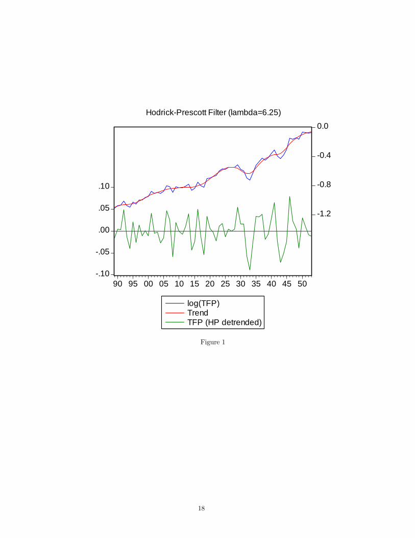
We Hodrick-Prescott detrend zt (as well as all other data) and specify the pa-rameter using the frequency power rule of Ravn and Uhlig (2002) (the numberof periods per year divided by 4, raised to a power, and multiplied by 1600).We find that this resulting series is well-described by a first order autoregressiveprocess with ρ = 0.77.First, we plot TFP in Figure 1. Compared to the other decades in the

sample, TFP experienced the highest growth during the 1920s. It was also theleast volatile, and the highest on average. In Figure 2 we plot simulated modeloutput compared to the data (both HP filtered). We adjust the volatility ofshocks so that output’s variance is the same for the model and the data overthe whole sample.3 The correlation between model and data is 0.85. Figure3 shows this data for the 1920s and 1930s, where the correlation is slightlylower, at 0.78. The model misses the start of the Great Depression — it comestoo late. We attribute this to the high TFP growth of the 1930s. The modelalso overestimates the speed of the recovery. This is consistent with Cole andOhanian’s (1999) recognition that changes in TFP cannot explain the weaknessof the recovery. However, over the 1920s the model does quite well. There werethree recessions, each lasting over a year, from 1920:I to 1921:III, 1923:II to1924:III and 1926:III to 1927:IV. The model matches these, and does particularlywell in the latter part of the decade. As with the other theories that we considerhere, we will conduct a quantitative analysis of the model’s performance inSection 4.5.

4.3 The SFE model

In this section, we use the SFE model (γ = 0.2). Here we have in mind anexplanation of the 1920s in line with Allen (1931):

”[The 1920s] represent nearly seven years of unparalleled plenty;nearly seven years during which men and women might be disil-lusioned about politics and religion and love, but believed that atthe end of the rainbow there was at least a pot of negotiable legaltender consisting of the profits of American industry and American

3The reasoning here is twofold. First, the volatility of the sunspot shock in the SFE modelis not pinned down, so a comparison of relative magnitudes is inappropriate. Second, ournumerical analysis is an examination of statistical significance and goodness of fit, so thatagain relative magnitudes are not relevant.

8

salesmanship [...] For nearly seven years the prosperity band-wagonrolled down Main Street.” (p 138)

In this case the model can be represented by:⎡⎣ bkt+1bzt+1bct+1⎤⎦ =MY

⎡⎣ bktbztbct⎤⎦+Mε

∙zt+1

ηt+1

¸(11)

Here ηt stands for expectational shocks or errors. Roughly speaking, given a se-quence of fundamental shocks to agents’ preferences and technologies, a solutionto this linear rational expectations model is a sequence of rational expectationsforecast errors under which the endogenous variables do not explode. Underindeterminacy the forecast errors can be decomposed in two components, one isdue to the fundamental shocks, and the other one is caused by sunspot shocks.(See, for example, Sims, 2000 and Lubik and Schorfheide, 2003.)Our procedure is similar in spirit to the business cycle accounting approach

that has been recently advocated by Chari, Kehoe and McGrattan (2007). Ina nutshell, they use an extended real business cycle model with various fric-tions (aka wedges) that are measured using various model equations (first orderconditions and the production function). Then these shocks are fed back intothe artificial economy in order to predict the fraction of cycles the frictions areable to account for. Unlike Chari, Kehoe and McGrattan (2007), here we test areal business cycle model with indeterminacy; i.e. we assume that the economyis best described by a model in which sunspots matter. Since the occurrenceof sunspots is not manifested by single first order equations but rather by thecomplete model i.e. a combination of the first order and side condition, ouraccounting must rely on the reduced form of our artificial economy.Now, we are ready to exploit the first rows of (10) and (14), which for our

calibration is:

Etbct+1 = −0.0768371bkt + 0.0183564bzt + 1.16526bct,as follows. We know that bct+1 −Etbct+1 = ηt+1 hencebct+1 = −0.0768371bkt + 0.0183564bzt + 1.16526bct + ηt+1.

This is sufficient to generate a theory consistent series of expectations from datain the following sense: the expectational shock is constructed by subtractingexpected consumption from the actual data.4 With indeterminacy, agents havemore information; and this new information is captured in the term ηt+1 which,given the environment, is a function of state of technology and the sunspot,ζt+1. We restrict the sunspot to be orthogonal to the fundamental disturbanceterm. Hence, we run a regression:

ηt+1 =bβ t+1 + ζt+1

over the complete annual sample period 1889 to 1953. (Again, data have beenhp-detrended.) Unlike the RBC model, we assume increasing returns and ac-cordingly, TFP is computed as

zt =yt

(utkt)0.36n0.84t

.

4Our procedure is similar to Salyer and Sheffrin (1998) however, we do not use stock marketdata to construct the sunspots. We did this in an earlier version of this paper; and we foundthat the so constructed shocks simply are essentially the stock market movements.

9

The regression’s residuals are plotted in Figure 4, and their values in the 1920sand 1930s in Figure 5. They are, of course, mean zero over the entire sample,while we see all shocks except one (1927) are positive during the 1920s. Thisindicates an optimistic attitude unrelated to fundamentals. This confidence mayin fact be a reflection of Allen (1931):

”The confidence had been excessive.”(p 250)

We see negative shocks starting in 1930, and a recovery in 1934. To makethe emerging picture clearer, we display an index of confidence constructed fromthe residuals over the sample, which is computed by chaining the measuredinnovations from year to year (a first-difference filter). This is in Figures 6 and7, for the entire sample, and then for just the 1920s and 1930s. In Figure 7 weplot it with output from the data. We clearly see that the level of confidencerises steadily throughout the twenties, while somewhat leveling off around 1925and plummeting after 1929. Furthermore, confidence makes a recovery aftera trough in 1933. Confidence falls again with the recession of 1937. Overall,confidence very much follows the pattern of US output. This echoes Allen(1931):

”Only when the memory of hard times has dimmed can confi-dence fully establish itself; only when confidence has led to outra-geous excesses can it be checked. It was as difficult for Mr. Hooverto stop the psychological pendulum on its down-swing as it had beenfor the Federal Reserve to stop it on its up-swing.” ( p 299)

In figures 8 and 9 we display model output and the data. The model outputis computed by feeding in only sunspot shocks, so that we can judge their efficacyalone. The standard deviation of the shock is again adjusted so that output’svariance is the same for the model and the data over the whole sample. Thecorrelations are 0.54 (whole sample) and 0.76 (20s and 30s). The model againcaptures the behavior of the 1920s quite well, especially after 1925. Note thatthis model better predicts the recovery from the Great Depression, due to therebounding confidence.

4.4 The MC Model

Use of this model is motivated in part by the evidence in Olney (1991) aboutthe credit expansion. She argues persuasively that the "consumer durablesrevolution" of the 1920s was accompanied by a significant expansion of credit:

”Debt for buying cars increased phenomenally in the 1920s, withnearly five times as much debt outstanding in 1929 as in 1922...Thecombination of all other goods debt also increased markedly in the1920s: it more than tripled.” (p 92)

This refers to nominal debt. She notes that many prices of consumer durableswere falling and that real measures reveal similar increases. Allen (1931) assertsthat by the 1920s

”people were getting to consider it old-fashioned to limit theirpurchases to the amount of their cash balances.” (p 168)

10

In addition, evidence about important changes in the banking industry dur-ing this time supports the use of this model. Wheelock (1992) cites the creationof so many new banks during the first two decades of the 20th century so as tolead to ”overbanking.” Consequently, the number of banks fell starting in themid-1920s, from 30,291 in 1920 to 24,970 in 1929, a fall of nearly 20%. He citesthe Federal Reserve Board as saying there were

”too many bank charters where there was no real need for them”(p 2)

He also cites the creation of deposit insurance for contributing to the prob-lem. Friedman and Schwartz (1963) concur:

”In an effort to attract banks to their respective jurisdictions,the state and national banking systems engaged in a competitiverelaxation of charter requirements and of the limitations imposed onbanking activities.” (p 240)

They also offer, along with Ginzberg (2004), how this affected lending anddeposits:

”The high prosperity of the twenties and the spreading belief ofa new era understandably led to an increasing optimistic evaluationof the prospects of repayment and hence to an increasing readinessto lend on a given project or collateral.” (Friedman and Schwartz, p246)

and

”Total deposits in all banks amounted to approximately 36 billiondollars in 1922 and 52 billion dollars in 1929. The annals record onlyone parallel increase...during World War I.” (Ginzberg, p 97)

Taken together, this points to (agnostically defined) positive productivityshocks in the banking sector during the 1920s.In addition, the state of monetary policy in the 1920s was as follows. Ac-

cording to Bernanke (2002), amidst concerns about the rising stock market,monetary policy failed to be corrective. Instead, it was accommodative. Onlyin 1928, when influential Governor of the Federal Reserve Bank of New YorkBenjamin Strong died, did the Fed begin to raise interest rates.Ideally we would like to use the intratemporal condition (10) to account for

the sequence of vt shocks. However, data for hours worked in banking sectoris not available before the 1970s. Moreover it is not clear how to measure at.Hence, following BGK, we estimate the shocks as follows.5 Recall the model’ssolution took on the form:bkt+1 = ∆1bkt +∆2zt +∆3vt +∆4ut

[Xt] = Λ1[bkt] + Λ2⎡⎣ zt

vtut

⎤⎦ ,5Thanks to Szilard Benk for assistance with this.

11

where the ∆ terms are scalars while Λ1 and Λ2 are matrices. One can estimatesequences of shocks using the least squares formulae⎡⎣ zt

vtut

⎤⎦ = (Λ02Λ2)−1 Λ02 ³[Xt]− Λ1[bkt]´ .Here we use HP filtered consumption, total hours worked, the GDP deflatorand GDP (all per capita) in [Xt] = [bct bnt bpt byt]. In our simulations, we producemodel output in two ways. First we include only credit shocks, and then onlymoney shocks. We call these the credit model and the money model. In neithercase do we include technology shocks. Again, our goal is to assess the role thatthese changes played in isolation.The results for the credit model are shown in Figures 10 and 11. Figure

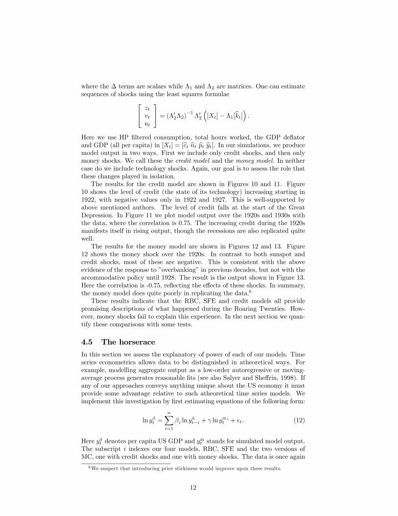
10 shows the level of credit (the state of its technology) increasing starting in1922, with negative values only in 1922 and 1927. This is well-supported byabove mentioned authors. The level of credit falls at the start of the GreatDepression. In Figure 11 we plot model output over the 1920s and 1930s withthe data, where the correlation is 0.75. The increasing credit during the 1920smanifests itself in rising output, though the recessions are also replicated quitewell.The results for the money model are shown in Figures 12 and 13. Figure

12 shows the money shock over the 1920s. In contrast to both sunspot andcredit shocks, most of these are negative. This is consistent with the aboveevidence of the response to ”overbanking” in previous decades, but not with theaccommodative policy until 1928. The result is the output shown in Figure 13.Here the correlation is -0.75, reflecting the effects of these shocks. In summary,the money model does quite poorly in replicating the data.6

These results indicate that the RBC, SFE and credit models all providepromising descriptions of what happened during the Roaring Twenties. How-ever, money shocks fail to explain this experience. In the next section we quan-tify these comparisons with some tests.

4.5 The horserace

In this section we assess the explanatory of power of each of our models. Timeseries econometrics allows data to be distinguished in atheoretical ways. Forexample, modelling aggregate output as a low-order autoregressive or moving-average process generates reasonable fits (see also Salyer and Sheffrin, 1998). Ifany of our approaches conveys anything unique about the US economy it mustprovide some advantage relative to such atheoretical time series models. Weimplement this investigation by first estimating equations of the following form:

ln ydt =nXi=1

βi ln ydt−i + γ ln ymi

t + t. (12)

Here ydt denotes per capita US GDP and ymt stands for simulated model output.

The subscript i indexes our four models, RBC, SFE and the two versions ofMC, one with credit shocks and one with money shocks. The data is once again

6We suspect that introducing price stickiness would improve upon these results.

12

HP-filtered. The idea behind conducting these tests is that by adding outputfrom a model to the regression, one obtains a measure of to what extent theparticular shocks in the model provide additional informational content.Let us begin with the autoregressive model. A lag length of n = 2 was

chosen since other lags were not significant. Furthermore, given the interestsof this paper, we restrict the analysis to the interwar period (1920-1939). TheAR(2) model is as follows (t-statistics in parenthesis)

ln ydt = 0.622(3.120)

ln ydt−1 − 0.489(−2.426)

ln ydt−2.

In the regressions reported in Table 1, we check to what extent contem-poraneous model realizations provide additional informational content. Eachline contains the results from one regression. Row 1 corresponds to the AR(2)process. Row 2 considers the RBC model, row 3 the sunspot model, row 4 thecredit model and row 5 the money model.We notice that the sunspot model provides the most information, reducing

the standard error of the regression by the most, and producing the highestadjusted R2. The RBC model is next, and the credit model follows closely. Thecoefficient for the money model is negative, for reasons similar to those explainedabove.

Table 1Regression results

Line Variable Coefficient R2

S.E.R. p-value(t-value)

1 - - 0.353 0.046 -2 yrbc 1.056∗

(3.818)0.631 0.035 0.001

3 ysun 1.076(3.872)

∗ 0.636 0.034 0.001

4 ycredit 0.795(3.292)

∗ 0.581 0.037 0.004

5 ymoney −0.569(−2.953)

∗ 0.547 0.038 0.009

Table 1 — Each line reports regression statistics of linearly detrended per capitaoutput on a constant and on own lags using annual data 1920 to 1939. Dependentvariable: loglinearly detrended per capita output. Coefficient = estimate when variableis added to regression, S.E.R. = standard error of regression, p-value = probabilityvalue of the null that the variable is zero. Row 1 corresponds to AR(2) process. Row2 considers the RBC model, row 3 the sunspot model, row 4 the credit model and row5 the money model. A * indicates significance at the 5% level.In order to further ascertain the additional power that each model provides,

we next estimate a horserace in the spirit of Fair and Shiller (1990). Our modelis:

ln ydt =nXi=1

βi ln ymit + t.

We estimate all the possible versions of this equation, including different models,in order to fully compare the explanatory power of each model above and beyondthat of the others. Table 2 summarizes. The money model continues to have a

13

negative coefficient throughout. When all models are included, the credit modelalso contributes negatively, though the coefficient is not statistically significant.When any other model (or models) is left out, the credit model’s coefficientis positive, but it is only significant on line 7. In other words, these resultsindicate that the credit model provides no statistically significant additionalhelp in explaining output above and beyond the other models in particularthe sunspot model. The results for the RBC model are better, with 5 outof 11 significantly positive coefficients. The sunspot model is the only onewith a significant coefficient in every regression. That is, it provides differentinformation than the other models in every case. From these tests, we concludethat the sunspot model provides the best description of the experience of theRoaring Twenties.

Table 2Regression results (t-values in parenthesis)Line RBC Sunspot Credit Money1 0.907∗

(3.203)0.598∗(3.485)

−0.495(−1.922)

−0.624∗(−4.862)

2 0.333(0.848)

0.724∗(2.792)

0.412(1.521)

-

3 - 0.855∗(4.535)

0.155(0.786)

− 0.452∗(−3.122)

4 1.369∗(4.248)

- −0.630(−1.923)

−0.691∗(−4.2233)

5 0.478∗(2.548)

0.648∗(3.547)

- −0.445∗(−4.677)

6 0.797∗(3.102)

0.699∗(2.610)

- -

7 - 0.823∗(3.583 )

0.591∗(3.480)

-

8 - 0.915∗(5.350)

- −0.533∗(−5.264)

9 0.828(2.01)

- 0.366(1.152)

-

10 0.860∗(4.361)

- - −0.465∗(−3.821)

11 - - 0.513(1.965)

−0.416(−1.989)

Table 2: Horserace regressions. Each line shows the results from a regression ofthe included variables. A * indicates significance at the 5% level.

Given that the RBC, sunspot and credit model provide the best explanatorypower, we next extend this analysis for these models to the period from 1890 to1939. The RBC and credit models each have positive and significant coefficientsin 2 of their 3 regressions. However, and most importantly, again only thesunspot model is significant in every regression. This evidence concurs with our

14

conclusion that the sunspot model provides the most explanatory power.

Table 3Regression results (t-values in parenthesis)Line RBC Sunspot Credit1 0.356

(1.851)0.514∗(3.296)

0.408∗(2.327)

2 − 0.627∗(4.254)

0.677∗(6.704)

3 0.725∗(6.435)

0.499∗(3.061)

-

4 0.602∗(3.098)

− 0.383(1.992)

Table 3: Horserace regressions 1890 to 1939. Each line shows the results from aregression of the included variables. A * indicates significance at the 5% level.

5 Summary and Conclusion”What is frustrating to economists is the conventional view: that

the economy was basically sound but that excessive speculation bythe public at large brought old-time American capitalism to grief.”[Hughes and Cain, 2007, 466]

In this paper, we have examined the ability of four different theories to ex-plain the experience of the 1920s. Technological innovation during the periodmotivated the use of the RBC model as a benchmark. At the same time, theexpansion of credit was clearly an important development during this period,enabling consumers to spend more than they earned. Of particular interestto us, however, are the results for the SFE model. Given the substantial ev-idence of persistent confidence not linked to fundamentals, and the results ofour horserace, we conclude that sunspot shocks were the primary driving forcebehind the Roaring Twenties. The logical next phase of this research projectis to produce a model in which both sunspot and credit shocks are relevant tothe workings of the economy.

References[1] Allen, F.L., 1931. Only Yesterday. New York: Harper & Row (2000 ver-

sion).

[2] Balke, Nathan S., Gordon, Robert J., 1986. Historical Data. In Gordon,Robert J. (Ed.). The American Business Cycle: Continuity and Change:Studies in Business Cycles Volume 25, National Bureau of Economic Re-search. Chicago: University of Chicago Press, 781-850.

[3] Basu, S., Fernald, J.G., 1997. Returns to scale in U.S. production: estimatesand implications. Journal of Political Economy 105, 249-283.

[4] Benhabib, J., Farmer, R.E.A., 1999. Indeterminacy and sunspots in macro-economics. In: Taylor, J.B., Woodford, M. (Eds.). Handbook of Macroeco-nomics, Vol. 1A. Amsterdam: North Holland, 387-448.

15

[5] Benhabib, J. and Wen, Y., 2004. Indeterminacy, aggregate demand andthe real business cycle. Journal of Monetary Economics, 51, 503-530.

[6] Benk, S., Gillman, M. and Kejak, M., 2005. Credit shocks in the financialderegulatory era: not the usual suspects. Review of Economic Dynamics 8,668-687.

[7] Bernanke, B.S., 2002. Asset-Price "Bubbles" and Monetary Policy.http://www.federalreserve.gov/BoardDocs/Speeches/2002/20021015/default.htm

[8] Bernanke, B.S. Parkinson, M.L., 1991. Procyclical labor productivity andcompeting theories of the business cycle: some evidence from interwar U.S.manufacturing industries, Journal of Political Economy 99, 439-459.

[9] Bordo, M.D., Erceg, C.J. and Evans, C.L., 2000. Money, sticky wages andthe great depression. American Economic Review 90, 1447-1463.

[10] Burns, A.R., 1936, The decline of competition (McGraw-Hill, New York).

[11] Chari, V.V., Kehoe, P.J. and McGrattan, E.R., 2007. Business cycle ac-counting. Econometrica 75(3), 781-836.

[12] Cole, H.L.,Ohanian, L.E. 1999. The great depression in the United Statesfrom a neoclassical perspective. Federal Reserve Bank of Minneapolis Quar-terly Review 23, 2-24.

[13] Cole, H.L.,Ohanian, L.E., 2001. New deal policies and the persistence ofthe great depression: a general equilibrium analysis. Federal Reserve Bankof Minneapolis Working Paper #597.

[14] Delong, J.B., 1997. Slouching Towards Utopia? The Eco-nomic History of the Twentieth Century, Chapter XIII.,econ161.berkeley.edu/TCEH/Slouch_roaring13.html.

[15] Fair, Ray C., Shiller, Robert J, 1990. Comparing information in forecastsfrom econometric models. American Economic Review 80(3), 375-89.

[16] Friedman, Milton and Schwartz, Anna J., 1963. A Monetary History ofthe United States,1867-1960. Princeton: Princeton University Press.

[17] Gillman, M., Kejak, M., 2005. Inflation and balanced-path growth withalternative payment mechanisms. Economic Journal 115, 247-270.

[18] Gillman, M., Otto, G., 2003. Money demand in a banking time economy.Discussion paper 254. Hamburg Institute of International Economics.

[19] Ginzberg, E, 2004. The Illusion of Economic Stability. Reprinted by Trans-action Publishers.

[20] Greenwood, J., Hercowitz, Z. and Huffman, G., 1988. Investment, capacityutilization, and the real business cycle. American Economic Review 78,402-417.

[21] Harrison, S.G. and M. Weder, 2006, Did sunspot forces cause the greatdepression? Journal of Monetary Economics 53, 1327-1339.

16

[22] Hughes, J. and L. Cain 2007. American Economic History, Pearson.

[23] Kendrick, J.W., 1961. Productivity trends in the United States. Princeton:Princeton University Press (for NBER).

[24] Lubik, T.A., Schorfheide, F., 2003. Computing sunspot equilibria in linearrational expectations models. Journal of Economic Dynamics and Control28, 273-285.

[25] Olney, M., 1991. Buy Now, Pay Later: Advertising, Credit and ConsumerDurables in the 1920s. The University of North Carolina Press.

[26] Prescott, Edward C, 1999. Some observations on the great depression. Fed-eral Reserve Bank of Minneapolis Quarterly Review 23, 25-31.

[27] Ravn, M. and H. Uhlig 2002. On Adjusting the HP-Filter for the Frequencyof Observations,” Review of Economics and Statistics 84, 371-76

[28] Salyer, K.D., Sheffrin, S.M. 1998. Spotting sunspots: some evidence insupport of models with self-fulfilling prophecies. Journal of Monetary Eco-nomics 42, 511-523.

[29] Sims, C., 2000. Solving linear rational expectations models. Unpublishedmanuscript, Princeton University.

[30] Weder. M. 2006. The role of preference shocks and capital utilization in thegreat depression, International Economic Review 47, 1247-1268.

[31] Wen, Y., 1998. Capacity utilization under increasing returns to scale. Jour-nal of Economic Theory 81, 7-36.

[32] Wheelock, D.C., 1992. Government policy and banking instability: "over-banking" in the 1920s. Federal Bank of St. Louis Working Paper 1992-007A.

17

-.10

-.05

.00

.05

.10

-1.2

-0.8

-0.4

0.0

90 95 00 05 10 15 20 25 30 35 40 45 50

log(TFP)TrendTFP (HP detrended)

Hodrick-Prescott Filter (lambda=6.25)

Figure 1

18

HP-filtered Output

-0.15

-0.1

-0.05

0

0.05

0.1

0.15

89 92 95 98 01 04 07 10 13 16 19 22 25 28 31 34 37 40 43 46 49 52

RBCUS data

Figure 2

19

HP-filtered Output

-0.15

-0.1

-0.05

0

0.05

0.1

0.15

20 21 22 23 24 25 26 27 28 29 30 31 32 33 34 35 36 37 38 39

US dataRBC

Figure 3

20

Sunspots

-0.08

-0.06

-0.04

-0.02

0

0.02

0.04

0.06

0.08

90 93 96 99 02 05 08 11 14 17 20 23 26 29 32 35 38 41 44 47 50 53

Sunspots

Figure 4

21

Sunspots

-0.05

-0.04

-0.03

-0.02

-0.01

0

0.01

0.02

0.03

0.04

20 21 22 23 24 25 26 27 28 29 30 31 32 33 34 35 36 37 38 39 Sunspots

Figure 5

22

99.84

99.88

99.92

99.96

100.00

100.04

90 95 00 05 10 15 20 25 30 35 40 45 50

Sunspot level

1929=100

Figure 6

23

99.88

99.90

99.92

99.94

99.96

99.98

100.00

-.15

-.10

-.05

.00

.05

.10

20 22 24 26 28 30 32 34 36 38

Sunspot level USA output (HP)

Figure 7

24

Output

-0.2

-0.15

-0.1

-0.05

0

0.05

0.1

0.15

90 93 96 99 02 05 08 11 14 17 20 23 26 29 32 35 38 41 44 47 50 53 US dataSFEmodel

Figure 8

25

Output

-0.15

-0.1

-0.05

0

0.05

0.1

0.15

20 21 22 23 24 25 26 27 28 29 30 31 32 33 34 35 36 37 38 39

US dataSFE model

Figure 9.

26

Credit shocks

-0.1

-0.08

-0.06

-0.04

-0.02

0

0.02

0.04

0.06

0.08

20 21 22 23 24 25 26 27 28 29 30 31 32 33 34 35 36 37 38 39

Figure 10

27

Output

-0.15

-0.1

-0.05

0

0.05

0.1

0.15

20 21 22 23 24 25 26 27 28 29 30 31 32 33 34 35 36 37 38 39

US dataCredit model

Figure 11

28

Money shocks

-0.06

-0.04

-0.02

0

0.02

0.04

0.06

0.08

20 21 22 23 24 25 26 27 28 29 30 31 32 33 34 35 36 37 38 39

Figure 12

29

Output

-0.2

-0.15

-0.1

-0.05

0

0.05

0.1

0.15

20 21 22 23 24 25 26 27 28 29 30 31 32 33 34 35 36 37 38 39 US dataMoney model

Figure 13

30