Technology Transfer and North-South∗

Martin Davies†

Department of Economics, Washington and Lee Universityand

Centre for Applied Macroeconomic Analysis, Australian National University

September 2015

Abstract

Costless technology transfer is a standard assumption in the international trade literature,however by some estimates the average technology transfer cost is nearly 20% of total projectcosts (Teece, 1977). This analysis examines the conditions under which the advanced countrygains when the transfer of technology from the advanced North to the less advanced South incursresource costs. Results are derived for the effect on production, wages, prices and welfare of lowertransmission and absorption costs, and productivity and population shocks. The framework isextended to examine the implications of an improvement in the enforcement of internationalintellectual property rights.

∗I wish to thank Peter Neary for excellent guidance during the writing of the thesis chapter upon which this paperis based. I am grateful to Richard Baldwin, Simon Cowan and an anonymous referee for very helpful comments.Conference participants at the Australian Conference of Economists 2011, Midwest International Economics GroupFall 2011, WTO Conference Jamia Millia Islamia University 2011, the Southern Economics Association Conference2010, and seminar participants at Washington and Lee University and the University of Papua New Guinea, areacknowledged. For assitance with the data section I thank George Nurisso, Daniel Rodriguez-Segura and StephenSmith.†daviesm@wlu.edu

1

1 Introduction and Motivation

To the joy of the anti-globalization lobby, and the chagrin of proponents of free trade, an influential

paper by Samuelson (2004) argues that the transfer of Northern technology directed to the Southern

importables sector facilitated by freer trade will diminish Ricardian comparative advantage and

with it the gains from trade. In the extreme, if the transfer equalizes relative labor productivities

between the North and South then the gains from trade are extinguished and welfare in the North is

lowered to its autarkic level, while the South with improved technology will gain.1 There have been

a number of responses to this dire possibility, and this paper is a further response. For example,

Jones and Ruffi n examine the conditions under which a country with superior technology may gain

when making an uncompensated transfer of superior technology to a less advanced country in both

2-good (Jones and Ruffi n, 2007) and n-good (Jones and Ruffi n, 2008) settings.

We extend the trade and technology transfer literature by examining the situation in which

there is an explicit resource cost of moving technology from one country to another within a general

equilibrium framework. The Ricardian continuum model of Dornbusch, Fischer and Samuelson

(DFS) is extended to allow for technology transfer from the North to the South, where Northern

resources are required to facilitate this transfer. Goods may now be produced in the South

using Northern technology which impacts production along two margins: it allows the adoption

of Northern technology by goods produced in the South, and it also allows the transfer of goods

production from the North to the South. The fall in the demand for Northern labor as goods (and

technology) relocate to the South is offset by an increase in the demand for Northern resources

in the transmission of technology. This source of demand is ignored when technology transfer is

assumed to be costless.

With this modification we examine the conditions under which technology transfer from the

North to the South will benefit the advanced country. Results are derived for the effect on

production, wages, prices and welfare of lower technology transfer costs, and productivity and

population shocks. We show that Northern welfare is likely to increase when technology transfer

is possible. We also show that Northern welfare in the technology transfer equilibrium is always

higher than the autarky equilibrium which results if technology transfer is costless. Further, while

an ongoing increase in the South’s relative labor supply may initially expand technology transfer,

1Dornbush, Fisher and Samuelson (1977) also note that the advanced country must lose when the harmonizationof relative unit labour requirements is complete.

2

it will eventually extinguish it as the relative price of Northern labor rises.

A common feature of the previous analyses is that there is no resource cost in the transfer

of technology. Whether through gift, theft or technological diffusion, productive factors in the

South are able to costlessly access and exploit Northern technology. In fact, the assumption that

technology can be transferred costlessly between countries is prevalent throughout the international

trade literature, an exception being Cheng, Qiu and Tan (2005).

However, technology transfer requires deliberate and costly action. Teece (1977) finds that

the average technology transfer cost is nearly one-fifth of total project costs, where the cost of

technology transfer is defined as the value of the resources which are required to transfer technology

from plants in one country to those in another. Following Teece, the activity of technology transfer

involves the transmission and absorption of technology, and resource costs associated with each of

these activities are mirrored in the structure of transfer costs in this paper. Absorption refers to

the ability of the recipient to assimilate new technology and hence these costs are bourne by the

South. Transmission costs, on the other hand, represent the cost of moving the superior technology

from one location to another, and primarily involve activities that engage resources in the advanced

country. To simplify the analysis we assume this to be the case.

Our extension has a number of advantages over analyses with costless technology transfer.

Firstly, the commodities in which technology transfer takes place are endogenously determined.

This differs from the two good analyses of Samuelson (2004) and Jones and Ruffi n (2007) in which

technology transfer from the North is directed to either the South’s exportable or importable

good, and the n-good model of Jones and Ruffi n (2008) in which technology transfer occurs in an

arbitrary good. Secondly, since technology transfer takes place in both the South’s exportable

and importable sectors, a shock which increases the ease of technology transfer leads to relocation

of production of some commodities along with their technology from the North to the South; and

also the exploitation of Northern technology by some, but not all, incumbent Southern exporters.

This differs from the Samuelson and Jones and Ruffi n analyses, which examine this shock as a

technology transfer to either the South’s importables or exportables sector. Thirdly, the transfer

of Northern technology creates a role for Northern expertise to assist in the application of superior

technology to Southern factors of production. This source of demand for Northern resources,

which occurs along two margins, is overlooked when the costs of technology transfer are assumed

away. When technology transfer leads to the relocation of production across borders, the requisite

3

transmission costs generate a demand for Northern factors of production. In addition, Northern

factors are required to assist producers in the Southern final good sector who choose to adopt

superior Northern technology. Both of these sources mitigate the reduction in demand for Northern

factors of production due to lost (relocated) production.

The resources engaged in technology transfer, and more generally in goods production, may be

thought of as an amalgam of capital, skilled and unskilled labor, and managerial services. Viewing

the single factor in this paper as a Leontief aggregate2 then this factor, which we call labor, may

be thought of as a productive resource encompassing all of these factors. The Ricardian model is

well suited to the analysis of technology transfer as technological differences, which are requisite

for technology transfer, form the basis for trade.

Three of the primary channels through which technology transfer occurs across international

boundaries are foreign direct investment (FDI), joint ventures, and licensing. While FDI is the

dominant channel for transfer of technology between developed and developing countries, and con-

tinues to grow in importance (Glass and Saggi, 2008) for the purpose of this paper we find no need

to distinguish between different modes of transfer. Regardless of the mode of transfer resource

costs must be incurred to move technology from one location to another.

Within this framework we examine the impact of lower absorption and transmission costs on

production, wages, prices and welfare. The impact on the technology transfer equilibrium of pro-

ductivity improvement in the final goods sectors of the South and the North, and also a population

shock, are also determined. There are a number of channels which may lead, through the conduits

of international trade and FDI, productivity levels between countries to be interrelated. We ex-

amine the possibility that technology transfer to the South might lead to spillovers, and establish a

condition to determine the equilibrium at which the total benefit from spillovers is maximized. Fi-

nally we examine impact of improved global enforcement of intellectual property rights on Northern

and Southern welfare.

This paper is organized as follows. Section 2 provides a brief examination of related literature.

Section 3 presents the model, and Section 4 provides analysis on the impact for a variety of shocks.

Section 5 examines the implications of technology transfer for prices and welfare and Section 6

provides some evidence on the empirical relevance of the model. Section 7 extends the model to

look at the effects of an improvement in intellectual property rights on welfare, and finally Section

2A Leontief aggregate is a fixed ratio of quantities.

4

8 concludes.

2 Literature

Samuelson (2004) examines the progression from autarky to free trade, and then the impact on

the free trade equilibrium of productivity shocks to the export and import sectors of the less

advanced country in a textbook two-good two-country Ricardian model using simple numerical

examples. While the productivity improvement in the export sector makes both countries better

off, the import shock makes the advanced country worse off. Jones and Ruffi n (2007, 2008)

examine the impact of an unrequited technology gift from an advanced home country with superior

technology to a less advanced foreign country. Jones and Ruffi n (2007), also using the textbook

Ricardian model, find that an unrequited transfer has the following implications. A transfer of the

import-competing technology will always benefit the home country as the pattern of comparative

advantage is maintained and the terms of trade improve. When the home country transfers all

of its technology to the foreign country there is no comparative advantage, and home’s welfare

falls to the autarkic level. Finally if the home country transfers the exportable technology, then

the pattern of comparative advantage is reversed. Since home has an absolute advantage in the

original importable, and unit labor requirements are equalized in the original exportable, then the

home country now has a comparative advantage in the original importable. The home country

may lose or gain from this situation.

In Jones and Ruffi n (2008) the impact of an uncompensated technology transfer suffi cient to

drive the advanced country out of producing its best export good is examined in an n-good two-

country Ricardian framework. When the equilibrium is located at a turning point such that

the advanced home country is incipiently producing a commodity, while the less advanced foreign

country supplies the entire world market of that commodity, then the relative wage is unaffected

by a transfer of technology. The advanced country now shares the market for that good with

the foreign country, which pins down the relative wage. The improvement in the foreign country’s

technology lowers the price level, leading to an increase in home’s real wage and welfare. When the

equilibrium is not at a turning point a transfer of technology will lead the foreign country’s wage

to rise. Although this leads to a fall in the price of the good whose technology was transferred,

the price of home’s other imports rises and the effect of home welfare is ambiguous.

5

Teece (1977) examines the determinants of the costs of transferring technology. Using data from

26 international technology transfer projects four groups of transfer costs are identified. These are:

i. cost of pre-engineering technological change; ii. engineering costs associated with transferring

the process design or product design; iii. costs of R & D personnel for adapting/modifying the

technology and solving unexpected problems during all phases of the transfer project, and iv. pre-

start-up training costs, and learning and debugging costs during the start-up phase. From the

sample, transfer costs average 19% of total project costs, with a range between 2% and 59%. Teece

makes a distinction between transmission and absorption costs which is mirrored in the structure

of resource costs of technology transfer in this paper. Absorption costs refer to the ability of

the recipient to absorb the new technology, which depend on both the recipient and host country

characteristics. When technology is complex and the recipient lacks the capacity to absorb the

new technology then the cost of transfer may be considerable. A related issue is whether resources

need to be devoted to building up absorptive capacity, as first discussed in Cohen and Levinthal

(1989). Leahy and Neary (2007) examine the theoretical implications of investment in absorptive

capacity.

The structure of the model in this paper is similar to that presented by Cheng et. al. (2005)

with a simple, yet significant, modification. While in Cheng et. al. the transmission of technology

is facilitated by an additional factor called expatriate workers which has no productive value in any

alternative use, and does not consume goods nor enter welfare calculations, here Northern labor is

engaged in this role. The resources used in the transmission of technology have an opportunity cost:

their value in the production of final goods in the North. The benefit of this modification is that the

model solves for a full general equilibrium. All productive activities including technology transfer

enter the relative demand for labor, and the relative supply of labor encompasses all resources.

Further, the boundaries which divide the goods continuum, between the South’s final goods sector,

the technology transfer sector and the North’s final goods sector depend on, and will respond to

changes in, the relative scarcity of labor.

Mussa (1978) examines the movement of capital between sectors when there is a resource cost to

do so in a two-good two-factor Heckscher-Ohlin-Samuelson economy facing external goods prices.

The resource cost includes intersectorally mobile labor and a factor specific to the capital movement

industry. The competitive adjustment path is determined in response to a price shock for both

static and rational expectations.

6

Krugman (1979) examines product cycle trade when innovations which create new products

occur at an exogenous rate in the developed North, and there is transfer of technology of new goods

from the North to the South also at an exogenous rate. The basis for trade is the technological lag,

with the North producing and exporting new products, and the South producing and exporting

only old products. Technology transfer is costless and once a blueprint becomes available to the

South, it is able to produce the good with productivity equal to that in the North.

Grossman and Rossi-Hansberg (2008), Baldwin and Robert-Nicoud (2007) and Rodriguez-Clare

(2010) all present models of offshoring of tasks. Tasks are the units of the building blocks of final

goods, and different factor-tasks are substitutable, reflecting factor substitution. Offshoring of a

particular task involves the application of home technology to cheaper foreign factors, and hence

these models make the assumption, whether implicit or explicit, that home technology may be

transferred, without explicit cost, for use by foreign factors.

3 Model

There is a continuum of goods on [0, 1], ordered according to increasing technological sophistication

with higher numbers indicating higher sophistication, as in Young (1991). Two countries, North

and South, are each endowed with a single productive factor called labor, LN and LS . For

simplicity, Southern labor is defined as the numeraire, and the relative price of labor, the North’s

wage, is defined as w. To facilitate its role in the transmission of technology Northern labor is

internationally mobile, while Southern labor is immobile.

3.1 Production

Production technology in the North and the South is defined as

yN (j) = LN (j)

yS (j) =LS(j)

a(j)

where units of goods are defined such that Northern unit labor requirements are unity for all j,

and a(j) represents the unit labor requirements for the South. It is assumed that the North has

an absolute advantage in all goods except the simplest, j = 0 : thus a (j) > 1 for all j > 0 and

a (0) = 1. In addition, the North has a comparative advantage in sophisticated goods, and a(j) is

7

increasing in j.

3.2 Technology Transfer Sector

Goods may be produced in the South using Northern technology. Similar to Cheng et. al. (2005),

to produce a good using Northern technology requires, in addition to an input of Southern labor,

an input of Northern labor which represents the transmission cost of technology transfer. The

Northern resource requirement for good j is aT (j) = γ + aT (j), with γ and aT (j) representing the

fixed and variable components of the transmission costs. The variable component, aT (j), has the

following properties:

i. aT (j) is continuous and twice differentiable in j,and a′T (j) > 0, a′′T (j) > 0.

ii. aT (0) = 0

iii. aT (1) > 1− γ

Property i. imposes that the transmission costs increase at a non-decreasing rate in sophistica-

tion. This is intuitive as the technology of more sophisticated goods is more complex, and transfer

of it requires more resources. Property iii. ensures in equilibrium that there is a Northern final

goods sector (z1 < 1). The unit labor requirement of Southern labor in technology transfer is

e = 1 + ε, where ε > 0 is the absorption cost. This reflects costs of production beyond Northern

technology, which has a unit labor requirement of one, since the South is unable to fully absorb and

exploit the technology from the North due to a lack of infrastructure, and language, cultural and

attitudinal differences. Technology is Leontief with a unit of good j requiring e units of Southern

labor and aT (j) units of Northern labor, and is represented by

y (j) = min

[LS (j)

e,LN (j)

aT (j)

](1)

with the unit cost of goods produced using transferred technology3

b(j) = 1 + ε+ waT (j)

3.3 Consumption

Households consume a continuum of final goods indexed by the variable j over the interval [0, 1]

and have identical homothetic preferences lnU =∫ 10 ln y(j)dj, where y(j) is the consumption of

3 In terms of the definition of the cost of technology transfer given by Teece (1977), waT (j) represents the trans-mission cost, and ε the absorption cost, both measured in units of Southern labour.

8

final good j. The consumer solves the problem maxy(j)∫ 10 ln y(j)dj subject to

∫ 10 p(j)y(j) = Y .

World demand for good j is(wLN + LS

)/p(j), where world income is wLN + LS . This leads to

the first result.

Lemma 1 The utility per capita is equal to the real wage, where ln(UN/LN

)= ln (w/P ) and

ln(US/LS

)= ln (1/P ) , where lnP =

∫ 10 ln p(j)dj is the true price index.

Proof. The proof is in the Appendix.

3.4 Technology Transfer Equilibrium

In order to ensure a well-behaved equilibrium we make the following two assumptions:

(A1) Single Crossing: a(z)− b(z) crosses zero only once, strictly from below.

a′(z0) >∂b(z)

∂z|z0 = wa′T (z0)

(A2) Convexity:4

d

dw

(dz0dw|dε,dγ=0

)=

d

dw

(aT (z0)

a′(z0)− wa′T (z0)

)> 0

Assumption (A1) ensures that technology transfer takes place over a contiguous interval of the goods

continuum. (A2) is required to establish an equilibrium, as will be demonstrated below. Assuming

perfect competition, the price of good j in the North is p(j) = w, and in the South is p(j) = a(j).

Goods may also be produced in the technology transfer sector at cost b(j) = e + waT (j). Given

the ordering of goods, and the assumptions about the resource costs of technology transfer, the

following two equations determine the boundaries of production location, z0 and z1.

a(z0) = b(z0) = e+ w (γ + aT (z0)) (2)

w = b(z1) = e+ w (γ + aT (z1)) (3)

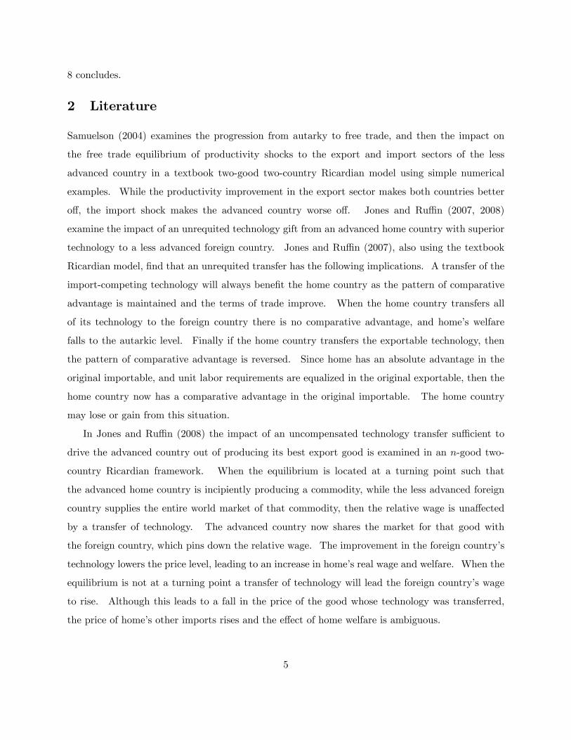
Production is allocated as demonstrated in Figure 1. The point α indicates the boundary between

the South’s final goods sector and the technology transfer sector, determined by (2) , and β indicates

the boundary between the technology transfer sector and the North’s final goods sector, determined

4This assumption requires that z1ww = 2a′T (z0) (a′(z0)− wa′T (z0)) − aT (z0) (a′′(z0)− wa′′T (z0)) > 0 which issatisfied when a′′(z0) 6 wa′′T (z0). When a (j) and aT (j) are linear in j, the inequality holds strictly as a′′ (j) anda′′T (j) are both zero.

9

jz1

α

w

1z00

a(j)b(j)

wT

1

β

e + wTγ

φ

Figure 1: Equilibrium with technology transfer

by (3). It follows that goods on the interval [0, z0) are produced in the South; goods on the interval

[z1, 1] are produced in the North; and goods on [z0, z1) are produced in the South using Northern

technology and both Northern and Southern labor. Because there is a resource cost of technology

transfer, transfer does not occur in goods for which comparative advantage is strongest: the simplest

goods for the South and the most sophisticated goods for the North.

3.5 Pre-technology Transfer Equilibrium

The Ricardian continuum framework forms the basis for part of the solution to the model, and also

represents the solution to the pre-technology transfer equilibrium, and is presented briefly. The

comparative advantage locus is

w = a(z) (4)

labor market equilibrium in the South is determined by LS = zwLN +zLS , which when rearranged

gives an equation for the balance of trade

w =

(1− zz

)λ (5)

10

where λ = LS/LN . This may be interpreted as the wage which ensures trade balance when the cut-

off good is z. At this point trade is balanced and the location of production is effi cient. Inverting

(4) so that z = a−1(w) = z(w) where z′(w) > 0 and substituting into (5) the equilibrium may be

expressed

w = hDFS (w) =

(1− z(w)

z(w)

)λ (6)

which is one equation in one unknown, w. For each value of λ ∈ (0,∞) there is a unique solution

to the DFS-benchmark model denoted by (zD(λ), wD(λ)). As λ increases the equilibrium wage

and cut off good, wD and zD, increase.

3.6 Balance of Trade with Technology Transfer

The South engages in two types of productive activity. It produces final goods on [0, z0) using

Southern technology, and it provides labor which is combined with Northern resources and tech-

nology to produce goods on [z0, z1). We separate the total demand for Southern labor into LSD1

and LSD2, corresponding to the sub-intervals [0, z0) and [z0, z1). The demand for Southern labor

to produce a good j on [0, z0) is LSD1(j) = a (j) y(j) = Y. The total demand for Southern labor

to produce goods j ∈ [0, z0) is LSD1 =∫ z00 Y = z0Y . On the interval [z0, z1) each unit of good j

requires the input of e units of Southern labor and aT (j) units of Northern labor according to (1).

Since the output of good j is y(j) = Y/ (e+ waT (j)) then the South’s derived demand for labor

for good j in the technology transfer sector is LSD2(j) = eY/ (e+ waT (j)). Integrating over [z0, z1)

yields

LSD2 = z1Y − z0Y − Y∫ z1

z0

waT (j)

e+ waT (j)dj

which gives the total demand for Southern labor in the technology transfer sector. We define for

convenience the following: θ(j) = waT (j) / (e+ waT (j)) and Θ(w, z0, z1) =∫ z1z0θ(j)dj, where θ(j)

is the North’s factor share in good j, and Θ(w, z1, z0) represents the North’s average factor share in

technology transfer.5 Equating the total demand for Southern labor, LSD1 + LSD2, with the supply

of Southern labor, LS , gives the South’s labor market equilibrium LS = (z1 −Θ(w, z0, z1))Y . This

may be written

w =

(1− (z1 −Θ(w, z0, z1))

z1 −Θ(w, z0, z1)

)λ (7)

5This is calculated as an arithmetic average where the weights are expenditure shares.

11

z

we/(1+ γ)

aT­1(1)

wH

zL

z0(w,ε,γ)

z1(w,ε,γ)

wL

zH

a­1(e)

wm

z0m

z1m

Figure 2: z0 (ω, ε, γ) and z1 (ω, ε, γ) when γ > γ and ε > ε∗ (γ)

and which determines the relative wage, w, which for given z0 and z1 yields balance of trade.6

3.7 Model with Technology Transfer

The model is expressed as three equations, (2) , (3), and (7) in three unknowns, w, z0, and z1.

Equations (2) and (3) may be used to determine the responses of z0 and z1 to changes in the

relative wage w, the absorption cost ε, and transmission costs γ. Applying (A1) it follows that7

z0 = z0(w+, ε+, γ+

) (8)

z1 = z1(w+, ε−, γ−

) (9)

From (A2), z0ww > 0 which ensures that z0 increases at a non-decreasing rate in w,8 and since

z1ww < 0 then z1 is increasing at a decreasing rate in w.

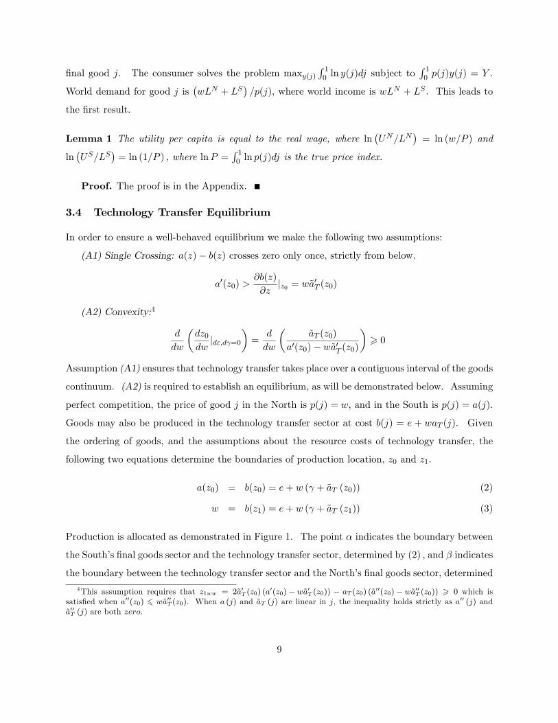
Using these properties the functions z0(w, ε, γ) and z1(w, ε, γ) are drawn in Figure 2 for given

6When there is no technology transfer, so that z1 = z0, then Θ(w, z0, z1) = 0 and the balance of trade reduces to(5).

7See the Appendix for calculation of these terms.8A suffi cient condition for (A2) is that a′′(z0) 6 wL′′T (z0)

12

ε and γ. Since z0ε > 0 and z1ε < 0 then as ε falls the z0(.) locus shifts to the left and the z1(.)

locus shifts to the right. Similarly since z0γ = w/ (a′ (z0)− wa′T (z0)) > 0 and z1γ < 0, a fall in

γ rotates the z0(.) upward around its vertical intercept z0 = a−1 (e) , 9 and shifts the z1(.) locus

right. Hence the impact of ε and γ have offsetting effects on the positions of the z0 (.) and z1 (.)

loci. For example, an increase in ε shifts the z0 (.) locus left and z1 (.) locus to the right, and a fall

in γ does the reverse.

Lemma 2 When ε = 0 the value of γ which ensures tangency between z0(w, ε, γ) and z1 (w, ε, γ)

is γ. For γ < γ there exists a value of ε > 0, defined as ε∗ (γ) at which there is tangency between

z0(w, ε, γ) and z1(w, ε, γ).

Proof. The proof is in the Appendix.

This result establishes that when ε and γ are zero then there is region of the goods continuum

where technology transfer will take place, and demonstrates the trade-off between γ and ε in terms

of their influences on the position of the z0(.) and z1(.) loci.

Lemma 3 When γ ≥ γ, or ε ≥ ε∗ (γ) for γ < γ, there is no technology transfer, and the solution

to the model is given by the DFS benchmark.

Proof. The proof is in the Appendix.

Under these parameter values the z0 (.) and z1 (.) loci are tangent, as in Figure 3, or non-touching

and technology transfer cannot occur.

Lemma 4 When γ ∈ [0, γ) and ε ∈ [0, ε∗ (γ)) there are two points of intersection between z0(w, ε, γ)

and z1 (w, ε, γ) on [0, 1), which are defined (zL (wL) , wL) and (zH (wH) , wH) . Associated with each

point of intersection is a relative labor endowment, λL (ε, γ) and λH (ε, γ) respectively. Conditions

for technology transfer require that γ ∈ [0, γ), ε ∈ [0, ε∗ (γ)) and λ ∈ (λL (ε, γ) , λH (ε, γ)) .

Proof. The proof is in the Appendix.

For technology transfer to take place, transmission and absorption costs together cannot be

too high and the relative labor supply cannot be too high or too low, lying within the ’Goldilocks’

region defined above, which is determined by ε and γ.

9Since at w = 0 then z0γ = 0.

13

z

w(1+ ε*) /(1+ γ)

aT­1(1)

z*

z0(w, ε*,γ)

z1(w, ε*,γ)

a ­1(1+ ε* )

w*

Figure 3: z0 (ω, ε, γ) and z1 (ω, ε, γ) when γ < γ and ε∗ (γ)

Definition 1 When γ ∈ (0, γ), ε ∈ (0, ε∗ (γ)) and λ is either λL(ε, γ) or λH (ε, γ) , or when

γ ∈ (0, γ), ε = ε∗ (γ) and λ∗ (ε, γ) , then technology transfer is incipient.10

In the first case the z0 (.) and z1 (.) loci intersect, and the relative labor supplies λL(ε, γ) and

λH (ε, γ) ensure equilibrium points such that technology transfer is just prevented. In the second

case z0 (.) and z1 (.) are tangent, as in Figure 3, and the relative labor supply λ∗ (ε, γ) ensures the

equilibrium point is at the point of tangency (z∗, w∗).

3.8 Solution of Model with Technology Transfer

Substituting (8) and (9) into (7) gives

w =

(1− (z1(w, ε, γ)−Θ(w, z0(w, ε, γ), z1(w, ε, γ)))

z1(w, ε, γ)−Θ(w, z0(w, ε, γ), z1(w, ε, γ))

)λ (10)

which is one equation in one unknown, w, and determines the equilibrium to the model when there

is technology transfer. Defining the RHS of (10) as hTT (w, ε, γ)λ, the equilibrium of the model is

10The value γ = γ is excluded from this definition because ε (γ) = 0 and it is not possible to examine a fall in εfrom ε = 0.

14

jz1

1

1z00

θ(j,w1 )

θ(j )

θ(j,w2)

dz1dz0

w2 > w1

a

b c

d

Figure 4: Representation of hTTω (ω, z0, z1)

determined by w = h (w, ε, γ)λ where

h (w, ε, γ)λ =

{hTT (w, ε, γ)λ for λ ∈ (λL (ε, γ) , λH (ε, γ))hDFS (w)λ for λ 6 λL (ε, γ) , λ > λH (ε, γ)

(11)

since from Lemma 4 the solution to the model is given by the DFS benchmark for λ 6 λL (ε, γ) , λ >λH (ε, γ). From Lemma 1, a unique equilibrium is ensured for λ on this range. To ensure

the existence of a unique equilibrium for λ ∈ (λL (ε, γ) , λH (ε, γ)) it is suffi cient to show that

hTTw(w, ε, γ) < 0 in the relevant range.

Unique Equilibrium A unique equilibrium is assured when an increase in the North’s relative

wage leads to an increase in the South’s share of world income, (z1−Θ), which is the denominator

of (10).11 As the wage increases there is adjustment to (z1 − Θ) on three margins. Firstly,

the North’s extensive margin, z1, contracts shifting goods into the technology transfer sector and

increasing the South’s share of world income by (1− θ(z1))z1w, represented by area d in Figure 4.

An increase in the wage also increases the extensive margin of Southern production, z0, which

moves goods from the technology transfer sector to the South and increases the South’s share of

11Since h (w, ε, γ) = (1− (z1 −Θ)) / (z1 −Θ) then sign|hw (w, ε, γ)| = −sign|z1w −Θw|. Hence hw (w, ε, γ) < 0requires z1w −Θw > 0.

15

h(w,ε,γ)λ

wwL

hDFS(w)λ

wH

hTT(w,ε,γ)λ

wT

h(wT,ε,γ)λ

hDFS (wL)λL

hDFS (wH)λH

Figure 5: Technology transfer equilibrium

world income by θ(z0))z0w (area b). Finally the rise in w decreases the South’s intensive margin in

the technology transfer sector which reduces the South’s share of world income by the third term

in (12) (area a). The overall effect on the South’s share of world income, and thus the relative

demand for Southern labor, of an increase in w depends on the sum of these terms

z1w −Θw = (1− θ (z1)) z1w + θ (z0) z0w −e

w

∫ z1

z0

θ (j)

b (j)dj (12)

The equilibrium locus hTT (w, ε, γ)λ is anchored at (wL, hDFS (wL)λL) and (wH , hDFS (wH)λH) ,

as drawn in Figure 5.12

It is also negatively sloped at these points because hTTw (wi, ε, γ) < 0 for i = L,H as the

third term in (12) is zero.13 For w ∈ (wL, wH) the third term in (12) is positive because there is

12This is drawn for the linear case (a (j) = 1 + j, b (j) = e+w (γ + j/2), which is interesting because hTT (w, ε, γ)λis steeper at both wL and wH and hence there is both a point on (wL, wH) where hTT (w, ε, γ)λ and hDFS (w)λintersect, and also a point of inflexion.13At (wi, hDFS (wi)λi) for i = L,H, since z0 = z1 = z then z1w − Θw = (1− θ(zi)) z1w + θ(zi)z0w > 0 and thus

hw (wi, ε, γ) < 0.

16

h(w,ε,γ)λ

wwL wHwT0

h(wT0,ε,γ)λ0

h(wT1,ε,γ)λ1 λ1> λ0

wT1

Figure 6: Effect of an increase in λ

technology transfer and z1 > z0, which leads to the possibility that hTTw (w, ε, γ) might become

positive for some w ∈ (wL, wH). We henceforth make assumption (A3) that z1w −Θw > 0 for all

w ∈ (wL, wH) which ensures a unique equilibrium. It is not possible to establish whether the slope

of hTT (w, ε, γ)λ is greater or less than the slope of hDFS (w)λ at wL and wH .14

4 Shocks

4.1 Population Shock

An increase in λ shifts the h(w, ε, γ)λ locus upward for any given w without altering wL or wH as

in Figure 6.15 The relative wage increases, and it follows from (8) and (9) that both z0 and z1

increase. The effect on the size of the technology transfer sector is examined in the next result.

Lemma 5 When ε ∈ [0, ε∗ (γ)) and λ ∈ (λL (ε, γ) , λH (ε, γ)) there exists a relative labor endow-

ment λm and a corresponding equilibrium (zm0 , zm1 , wm) at which technology transfer is maximized.

14At wi (i = L,H) it is the case that hDFSw (wi) = −z′ (wi) /z (wi)2 and hTTw(wi, e) =

− ((1− θ(z)) z1w + θ(z)z0w) /z (wi)2. At wL, z1w (wL) > z′ (wL) > z0w (wL) and at wH , z1w (wH) < z′ (wH) <

z0w (wH). Since vw is a weighted average of z1w (w) and z0w (w) , it is not possible to determine at either of thesepoints whether (1− θ(z)) z1w + θ(z)z0w T z′ (wi).15The points wL and wH are determined purely by technology and are not influenced by the demand side.

17

Proof. The proof is in the Appendix.

This equilibrium is drawn in Figure 2. At one extreme, when Northern labor is relatively

abundant and the North’s relative wage is very low, it is cheaper for the North to produce all

goods above z0 than to engage Southern labor in technology transfer. At the other extreme, when

Northern labor is very expensive it is cheaper for the South to produce all goods below z1 rather

than to employ Northern labor in the technology transfer sector.

If population growth in the South is higher than in the North (λ is increasing) this drives

up the price of Northern labor, pushing up z1 and z0. As λH is approached z1w is falling and

z0w is increasing and the size of the technology transfer sector, z1 − z0, is contracting. At λH

the relative wage has risen enough to extinguish technology transfer. This result runs counter

to mercantilist intuition, which might be stated as something like more abundant Southern labor

increases the incentive for the North to direct resources to transfer technology to the South to exploit

the opportunities created by cheaper Southern labor. This result is also counter to Corollary 1 in

Cheng et. al. (2005, p. 486), which states that as λ increases technology transfer becomes more

likely although this is under the condition that the factors engaged in the transmission of technology

are supplied at a fixed price.

As the Southern labor force expands the opportunity cost of the resources used in technology

transfer, measured by North’s relative wage, rise increasing the cost of producing goods using

technology transfer, and encouraging production of final goods in the South using Southern labor

and technology. Thus, for technology transfer to occur the relative labor supply must lie within the

’Goldilocks’region, λ ∈ (λL, λH). When the relative labor supply is too high or too low technology

transfer will not take place.

4.2 Improvement in Technology Transfer

Proposition 1 When technology transfer is incipient a reduction in the costs of technology transfer

(a fall in ε or γ) leads to technology transfer.

Proof. The proof is in the Appendix.

Corollary 1 When γ ∈ (0, γ) and ε ∈ (0, ε∗ (γ)), and λ ∈ [λL(ε, γ), λM (ε, γ)] , a reduction in the

absorption costs, ε, leads to an increase in technology transfer.

Proof. The proof is in the Appendix.

18

The effect on the relative wage of a fall in transmission or absorption costs is ambiguous. In

the remainder of this section we normalize the absorption and transmission shocks so that they

have equal measure in terms of the numeraire, and therefore cause the same initial shock. This

allows us to make a comparison of impact on the term of trade of an absorption shock relative to

a transmission shock. Since b (j) = 1 + ε + wγ + waT (j) then a given change in γ will cause a

bigger vertical shift in the b (j) schedule than an identical change in ε because w > 1 in equilibrium.

Setting dε = wdγε ensures that the shocks shift the b (j) schedule vertically by the same distance.

We begin by demonstrating the effect on the relative wage of a fall in absorption costs. From (11)

it follows thatdw

dε=

λhTTε (w, ε, γ)

1− λhw (w, ε, γ)for λ ∈ (λL (ε, γ) , λH (ε, γ))

From (10) the effect on the relative wage depends on the impact of a change in ε on the South’s

share of world income, with sign |dw/dε| = -sign |z1ε −Θε| where

z1ε −Θε = (1− θ(z1)) z1ε + θ(z0)z0ε +

∫ z1

z0

θ (j)

b (j)dj (13)

For a fall in absorption costs the South’s extensive margin, z0, falls and goods initially produced

entirely in the South shift to the technology transfer sector reducing the South’s share of world

income by θ (z0) z0ε, which is represented by area t in Figure 7.

The North’s extensive margin also contracts (z1 rises) and goods that were initially produced

entirely in the North shift into the technology transfer sector, to be produced by both the North

and the South. This increases the South’s share of world income by − (1− θ (z1)) z1ε > 0 (area

q and first term in (13)). The fall in ε reduces the South’s intensive margin in the technology

transfer sector reducing the South’s share of world income (third term in (13), area r). Whether

the South’s share of income, and the relative demand for Southern labor, rises or falls as ε falls

depends on the sum of these terms in (13).

When transmission costs fall by dγε the effects on the extensive margins are identical however

the South’s intensive margin expands, represented by area x, which increases z1 − Θ and also

increase the demand for Southern labor. In this case the effect on the South’s share of world

income is measured by16

z1γε −Θγε = z1ε −Θε − w∫ z1

z0

1

b (j)

16Since the shocks are normalized (wdγε = dε) then z0γε = z0ε, and z0γε = z1ε.

19

j

1

1z00

θ(j,ε1,γ)

dz0 dz1

θ(j )

θ(j,ε2,γ)

ε1 > ε2γ1 > γ2

z1

t

q

r

sθ(j,ε,γ2)

x

Figure 7: Effect of a change in ε and γ on z1 −Θ

It follows that a fall in transmission costs reduces the relative demand for Northern labor more, or

increases it less, than a fall in the absorption cost, as the next result states.

Corollary 2 Comparing the impact on the relative wage of a fall in transmission costs relative to

a fall in absorption costs, it is the case that dw/dγε > dw/dε, where

dw

dγε=dw

dε− 1

∆

λ

(z1 −Θ)21

z0ε

1

z1ε

(∫ z1

z0

1

b (j)dj

)Proof. The proof is in the Appendix.

When the shocks are normalized the initial impact on the extensive margins is the same while

the effects on the intensive margins differ. A fall in absorption costs reduces the South’s intensive

margin while a fall in transmission costs expands it. Hence a fall in transmission costs leads to a

smaller rise, or a larger fall, in w than a fall in absorption costs which has the same initial impact.

Corollary 3 When technology transfer is incipient an improvement in absorption [lower ε], or a

fall in transmission costs [lower γ], will lead to an increase (decrease) in w if

z1εz0ε

< (>)− θ (z)

(1− θ (z))

20

Proof. The proof is in the Appendix.

In this case there is no adjustment on the intensive margin because initially z0 = z1. For a

fall in ε, or a fall in γ where dε = wdγε, the South’s extensive margin contracts and goods shift

out of the South’s final goods sector and into the technology transfer sector, which reduces the

the South’s share of world income by θ(z)z0ε. Similarly the North’s extensive margin contracts

which increases the South’s share of world income by − (1− θ (z)) z1ε. Thus, whether the relative

demand for Southern labor rises or falls depends on − (1− θ(z)) z1ε − θ(z)z0ε ≷ 0.

Corollary 4 When dε = wdγε, the effects of fall in absorption or transmission costs on Northern

and Southern welfare are as follows

dWN

dζ= (z1 −Θ)

d lnwTdζ

−∫ z1

z0

1

b (j)dj for ζ = ε, γε (14)

dWS

dζ= − (1− (z1 −Θ))

d lnwTdζ

−∫ z1

z0

1

b (j)dj for ζ = ε, γε (15)

where W i is the utility per capita in country i.

Proof. The proof is in the Appendix.

The first term in the expressions above is the terms of trade effect which is the percentage

change in the terms of trade weighted by the import share. These are opposed between the North

and South. The second term, which is defined as the effi ciency effect, represents the fall in prices of

goods produced in the technology transfer sector as transfer becomes more effi cient, either because

of a fall in ε or γ. It is possible that a fall in transfer costs will make both countries better off.

From Corollary 2, the North will be relatively better off from a fall in absorptions costs than from

a fall in transmission costs.

Since lnPT = − lnWST then the effect on the price level of a change in absorption or transmission

costs is given by the negative of (15). The interpretation is the same as that given above. For

example, when d lnwT /dζ < 0 then a fall in ε or γ leads to opposing effects on the price level. The

prices of goods produced in the North, and of Northern inputs into the technology transfer, rise

putting upward pressure on the price level, and more effi cient technology transfer puts downward

pressure on the price level.

21

4.3 Productivity Shocks

Proposition 2 (Southern catch-up) When there is technology transfer (z1 − z0 > 0), a proportional

catch-up in the productivity of the Southern final goods sector leads to an increase in the South’s

relative wage. In addition, when λ 6 λm, or when λ > λm and z0w − z1w < (z1 −Θ)2 /θ (z0)λ, it

leads to a contraction in technology transfer.

Proof. The proof is in the Appendix.

A proportional Southern productivity improvement shifts the z0 (.) locus upward, as may be

visualized in Figure 2. The impact of this at the initial wage is to reduce the size of the technology

transfer sector. Since the productivity improvement causes w to fall then when w 6 wm (λ 6 λm)

it follows that z1−z0 is reduced further. However, when w > wm (λ > λm) if z0w−z1w is large then

the range of goods produced in the technology transfer sector may rise as w falls. The condition

above places a restriction on the magnitude of z0w − z1w to ensure the result.

The intuition of this result is as follows. A proportional productivity catch-up means that

the a (j) schedule rotates downward around the vertical intercept a (0) = 1 as the productivity

of Southern final goods producers improves in proportion to their distance from the Northern

benchmark of unity, as in Figure 8. The productivity of Southern firms producing good 0, who are

as productive as their Northern counterparts, doesn’t change. This is modeled as a fall in South’s

productivity parameter, ρS , (from an initially value of unity) where the condition determining the

South’s extensive margin z0 is 1 + ρS (a (z0)− 1) = e+waT (z0). This shifts z0 to the right at the

initial wage because production costs fall in that sector increasing the relative demand for Southern

labor. This pushes down the North’s relative wage shifting the b (j) schedule down, decreasing

z1 and expanding Northern final goods production. The movement between the initial and final

equilibria are demonstrated in Figure 8, with the final equilibrium given by (w∗T , z∗∗0 , z

∗1) .

Corollary 5 The effects of a proportional catch-up in the productivity of the South’s final goods

sector on Northern and Southern welfare are as follows:

dWNT

dρS= z1

d lnwTdρS

−(z0ρS− 1

ρS

∫ z0

0

1

1 + ρS (a (j)− 1)dj

)R 0 (16)

dWST

dρS= − (1− z1)

d lnwTdρS

−(z0ρS− 1

ρS

∫ z0

0

1

1 + ρS (a (j)− 1)dj

)< 0 (17)

Proof. The proof is in the Appendix.

22

jz1

w

1z00

a*(j)b(j,wT)

wT

1

e + wTγ

a(j)

z0*z0

** z1*

wT*

e + wT*γ

b(j,wT* )

Figure 8: Proportional catch-up in South’s final goods sector

The first term in the expressions (16) and (17) are the terms of trade effects, which are opposed.

The second term in both expressions is the effi ciency effect and represent the fall in prices of goods

produced in the South due to the improved productivity. From (48), d lnwT /dρS > 0 and the terms

of trade move in favour of the South. An improvement in Southern final goods technology leaves

the South better off and the effect on Northern welfare, where the terms of trade and effi ciency

effects oppose, is ambiguous.

If the South continues to experience a proportional technological catch-up, eventually technology

transfer is extinguished, and the DFS equilibrium results.17 In the limit if the proportional catch-

up continues, then ρS approaches zero and the South’s technology approaches that of the North in

all goods (a (j) approaches unity for all goods j), and the equilibrium approaches autarky.

Proposition 3 (North leaps ahead) When there is technology transfer (z1 − z0 > 0), a uniform im-

provement in the productivity of the Northern final goods sector leads to an increase in the North’s

relative wage. In addition, when λ > λm, or when λ < λm and z1w−z0w < (z1 −Θ)2 / (1− θ (z1))λ,

it leads to a contraction in technology transfer.

17Note that from (44) , the vertical intercept of the z0 (.) locus is determined by z0 = a−1((ε+ ρS

)/ρS

). As ρS

falls then the z0 (.) locus shifts upward.

23

jz1

w

1z00

a(j)b(j,wT

* )

ρNwT

1

e + wT* γ

z0* z1

*

ρN*wT*

e + wT γ

b(j,wT )

ρN* < ρN

wT* > wT

Figure 9: Effect of uniform productivity improvement in North’s final goods sector

Proof. The proof is in the Appendix.

A uniform productivity improvement in the North shifts the z1 (.) locus downwards. This is

represented by a fall in ρN , the productivity in the North’s final good sector, from an initial value

of unity.18 At the initial wage this reduces the size of the technology transfer sector. Because the

wage rises then for w > wm (λ > λm) the technology transfer sector contracts further. However for

λ < λm the effect of the increase in w acts counter to initial impact on the size of the technology

transfer sector because z1w > z0w, and a restriction must be placed on the size of z1w − z0w to

ensure the result.

A uniform productivity improvement in Northern final goods sector shifts the z1 margin to the

left at the initial wage because production costs fall in that sector. This increases the relative

demand for Northern labor as goods produced originally in the technology transfer sector on that

margin release Southern labor and are now produced only in the North. This bids up the relative

wage, and z0 increases and z1 decreases. The movement between the initial and final equilibria

are demonstrated in Figure 9 (with post-shock variables indicated by an *).

Corollary 6 The effect of a uniform improvement in the productivity of the North’s final goods

18The North’s extensive margin, z1, is determined by ρNw = e+ waT (z1) .

24

sector on Northern and Southern welfare is as follows:

dWN

dρN= z1

d lnwTdρN

− (1− z1)ρN

> 0 (18)

dWS

dρN= − (1− z1)

d lnwTdρN

− (1− z1)ρN

T 0 (19)

Proof. The proof is in the Appendix.

The interpretation of (18) and (19) is similar to the case above, except that the effi ciency effect

is now over the range of goods [z1, 1], as opposed to [0, z0) in the previous case. From (61) the

terms of trade move in favour of the North, and the North is always better off while the effect on

Southern welfare is ambiguous.

5 Welfare and Prices

In this section we examine the impact on prices and welfare of the movement between the free trade

(DFS) and technology transfer equilibria.

5.1 Global Welfare

Lemma 6 Technology transfer leads to an increase in world real income, which is determined by19

ln

(YTPT

)− ln

(YDPD

)u∫ zD

z0

(ln a (j)− ln b(j)) dj +

∫ z1

zD

(lnwT − ln b(j)) dj > 0

where Yi/Pi is world income deflated by the price index Pi, for i = T,D.

Proof. The proof is in the Appendix.

In the movement from the free trade to the technology transfer equilibrium world welfare in-

creases. From a world perspective the terms of trade effects between countries are internalized.

The two terms on the RHS represent the effi ciency gains due to the transfer of technology from

North to South: the first term because of the transfer of technology to Southern incumbent pro-

ducers on [z0, zD), and the second term because technology transfer which has stimulated Southern

entry into goods on [zD, z1). Both terms are positive since a (j) > b(j) on [z0, zD) and wT > b(j)

on [zD, z1).

19The subscript D denotes the DFS benchmark (pre-technology transfer situation), and the subscript T denotesthe technology transfer situation.

25

5.2 Welfare in the North and South

The change in welfare per capita in the North is

∆WNT−D = zD ln

wTwD

+

∫ zD

z0

(ln a (j)− ln b (j)) dj +

∫ z1

zD

(lnwT − ln b (j)) dj (20)

The first term is the terms of trade effect and the second and third terms are the effi ciency gains

noted above. If the terms of trade were to move very strongly against the North it is possible

this loss would outweigh the effi ciency gains. Such an adverse movement is unlikely as the fall in

demand for Northern labor due to relocating goods is offset by higher demand in the transmission

of technology, and it is likely that the North will be better off than under free trade.

If transmission and absorption costs are zero, as in Samuelson (2004), then the South is able

to perfectly absorb all Northern technology, and relative (and absolute) labor productivities are

equalized at unity for all goods. Comparative advantage is eliminated, and welfare in the North

is driven back to its autarkic level. As we demonstrate in the next result, Northern welfare in the

technology transfer equilibrium is always above the autarkic level.

Lemma 7 The North is better off in the technology transfer equilibrium than under autarky, since20

∆WNT−A = WN

T −WNA =

∫ z0

0(lnwT − ln a (j)) dj −

∫ z1

z0

(lnwT − ln b(j)) dj > 0

Proof. The proof is in the Appendix.

The resource costs of technology transfer make it uneconomic to transfer technology in all goods,

and it will occur only on a fraction of the goods continuum [z0, z1). For goods above and below

this interval relative effi ciencies are unchanged. The first term above is the gains due to final goods

trade with the South, and the second term is the gains from trade attributed to the technology

transfer sector.

If transmission and absorption costs were to fall to zero the South has Northern technology and

is in autarky. We show below that the South would be better off in this situation than in the

technology transfer equilibrium.

Lemma 8 The South is better off when technology transfer is costless, in which case it has Northern20The subscript A indicates the autarkic equilibrium.

26

technology and is in autarky, than when technology transfer is costly since

WST −WS

A∗ = −(1− z1) lnwT −∫ z0

zA

ln a (j) dj −∫ z1

z0

ln b (j) dj < 0

Proof. The proof is in the Appendix.

5.3 Prices

The difference between the price level in the post- and pre-technology transfer equilibria is

lnPTPD

= (1− zD) lnwTwD−∫ zD

z0

(ln a (j)− ln b (j)) dj −∫ z1

zD

(lnwT − ln b(j)) dj (21)

The first term represents the change in the prices of goods on [z1, 1] which depends on the movement

of the terms of trade, wT /wD, and may be positive or negative. The second and third terms

represent the effi ciency gains, which will lower prices. The change in the price level between the

post- and pre-technology transfer equilibrium is ambiguous. Since WSi = − lnPi for i = D,T ,

then the change in Southern welfare between the post- and pre-technology transfer equilibrium is

∆WST−D = lnPD/PT .

6 Empirical Evidence on Technology Transfer

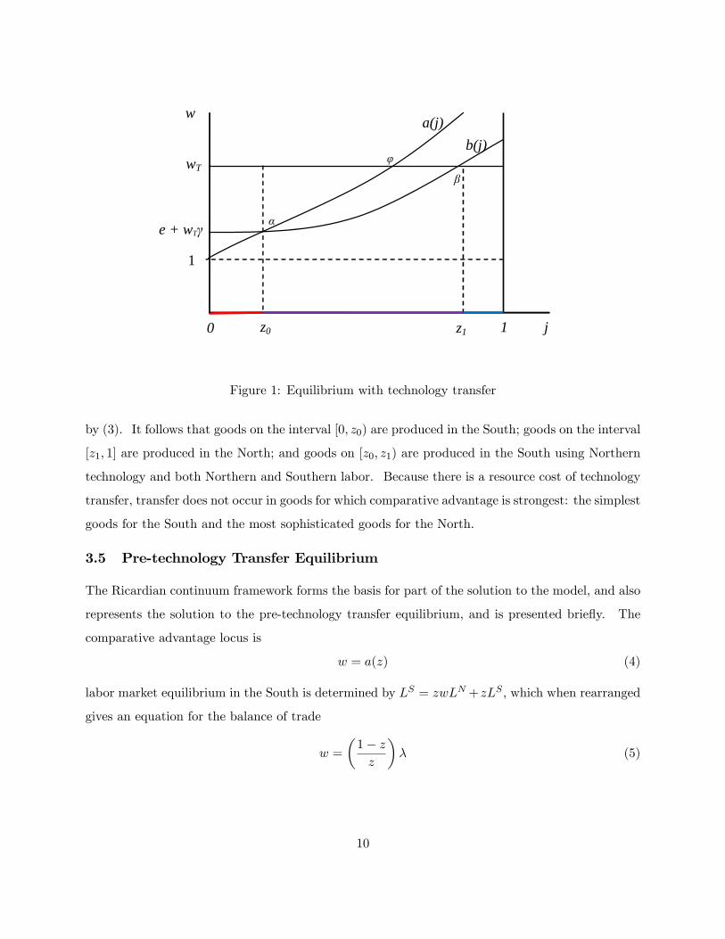
To demonstrate the relevance of this model we examine some simple empirics. Since FDI is a

primary channel through which technology transfer takes place, we use FDI flows between developed

and developing economies as a proxy for technology transfer. Our goal is to explore the pattern

of correlation between FDI flows and the level of development of countries, which we proxy by

gross domestic product (GDP) per capita. Recalling that labor in the model above is a Leontief

aggregate, then the wage is a measure of GDP per capita. While countries with high GDP per

capita generally have relatively advanced technology there are exceptions, for example some oil

exporters. In the second analysis below we use the IMF’s classifications of advanced country and

developing country, which takes this into consideration, to determine which countries belong to the

North and the South.21

We undertake two simple analyses: firstly, we examine the correlation between country net FDI

inflows, which is the difference between FDI inflows and outflows, and country GDP per capita;

21The IMF considers both GDP per capita and export diversification, so countries with high GDP per capita as aresult of oil exports are not counted as advanced.

27

and, secondly we divide countries into advanced and developing and examine the pattern of FDI

flows between Northern and Southern countries.

To begin we construct the following measures for each country: fi =(FDIInflowi − FDIOutflowi

)/FDIWorld

which is the net inflows of FDI into country i as a proportion of world FDI, and yi = Yi/Y , which

is the ratio of country i’s GDP per capita (Yi) to the average GDP per capita for our sample of

countries (Y ).22 For FDI data, we use the UNCTADSTAT FDI database which lists information

on FDI inflows and outflows for each country, and GDP data comes from the World Bank tables.

We have 12 years, from 2001-2012, of annual data and 193 countries. With data gaps there are

2049 observations of a possible 2316. Using standard OLS, we regress fi on yi and obtain the

following results

fi = 0.002(0.000)

− 0.001(0.000)

yi (R2 = 0.005)

While GDP per capita is not a perfect measure of development, as noted above, with a positive

constant and a negative slope this regression demonstrates that advanced (high GDP per capita)

countries are net exporters, and developing countries are net importers, of FDI. Since world net

FDI inflows must sum to zero by definition then Southern countries must be net recipients of FDI

from Northern countries.

In our second analysis, we examine the 50 largest countries as measured by GDP in the 2014

IMF World Economic Outlook, which account for approximately 80 percent of world FDI flows.23

For these countries, there is a natural equal split between advanced (Northern) and developing

(Southern) countries with 25 in each group. The UNCTADSTAT FDI database also lists for

each country the division of flows to and from developed, developing and transition, economies.

We group transition economies with developing economies, which brings the IMF and UNCTAD

classifications into close alignment.24 Defining FDIInflowNiSas the FDI inflows into Northern country

i from the South, and FDIOutflowNiSas the outflow from Northern country i to the South, then the

net FDI inflow from the South for Northern country i as a proportion of total 50 country FDI is

fNiS = (FDIInflowNiS−FDIOutflowNiS

)/FDI50.25 Similarly the net inflow from the North for Southern

country i as a proportion of total FDI is fSiN = (FDIInflowSiN− FDIOutflowSiN

)/FDI50. For all

22FDIWorld is the simple average of total FDI inflows and FDI outflows for the entire sample of countries.23 In fact, we look at the top 51 countries but exclude Taiwan because of data unavailability for some key variables.24The classifications aligns as follows: IMF advanced country with UNCTAD developed country; IMF developing

country with UNTCAD transition plus developing countries. One notable difference is South Korea which is advancedaccording to the IMF and developing according to UNCTAD.25Again, FDI50 is average of the sum of FDI inflow and outflows for the 50 countries examined.

28

countries we define GDP per capita as a proportion of the average GDP per capita of the top 50

countries, yki = Yki/Y50, where k = N,S, and Y50 is the average GDP per capita of the top 50

countries.

We have the same 12 years of annual data and 25 Northern and Southern countries. There are

gaps in the data with 187 observations for the South and 292 for the North, both out of a possible

300. To establish the pattern of correlation for the North, using OLS, we regress fNiS on yNi and

find that

fNiS = −0.003(0.002)

− 0.001(0.001)

yNi (R2 = 0.008)

Since both the constant and slope are negative, then on average Northern countries are net exporters

of FDI to Southern countries, and richer Northern countries have bigger net exports. To be clear,

in all of this analysis we are making statements only about correlation, not causality. Similarly for

the South we regress fSiN on ySiand find that

fSiN = 0.004(0.001)

+ 0.001(0.001)

ySi (R2 = 0.010)

With positive constant and slope then on average Southern countries are net importers of FDI,

and richer Southern countries have higher net imports of FDI.26 See Figure 10 for a graphical

presentation of these results.

7 Technology Transfer and Intellectual Property Rights

In the above analysis it is assumed that the blueprints for the Northern technology are freely

available and can be accessed at zero cost. The model is modified to examine the case where a

licence fee must be paid to use Northern technology. We now interpret γ as a licence fee which is

charged for each unit of goods produced using Northern technology by both Southern and Northern

firms. The licence fee is a rent paid to Northern workers, who are the owners of the advanced

technology. While the imposition of a licence fee increases the cost of producing goods using

Northern technology, it does not affect the resources required to produce them. There is now a

mark-up on goods on [z1, 1] . The cost of producing goods in the Northern final goods sector is

now w (1 + γ) and (3) becomes w = e+waT (z1) which is independent of γ, while (2) is unchanged.

The payment to Northern workers for the use of advanced technology is the total volume of goods26This is not only because richer Southern countries are bigger, but perhaps also because they have better institu-

tions and infrastructure.

29

Figure 10: Net FDI Inflows for Northern and Southern Countries, 2001-2012

on [z0, 1] multiplied by the licence fee γ. The share of world income paid as licence fees is

φ =

((1− z1) γ(1 + γ)

+(

Θ (w, z0, z1)− Θ (w, z0, z1)))

(22)

where Θ (w, z0, z1) =∫ z1z0

(waT (j) /b (j)) dj is the average factor share of Northern labor in technol-

ogy transfer while Θ (w, z0, z1) =∫ z1z0

(w (γ + aT (j)) /b (j)) dj is the average factor share including

license fee payments. The first term in (22) represents the share of world income paid as license

fees for goods produced in the North’s final goods sector, while the second term represents the share

for goods produced in the technology transfer sector. Because preferences are homothetic the equi-

librium is independent of the distribution of license fee revenue amongst the Northern workforce,

however for the purposes of this analysis we assume it to be equally shared. The income of a

Northern worker is the wage plus an equal share of the license fee payments, w + φY/LN . World

income is now27 Y =(wLN + LS

)/ (1− φ) and substitution of this into the South’s labor market

equilibrium condition, LS = (z1 −Θ)Y, leads to an expression for the balance of trade,

w =1− φ− (z1 −Θ)

(z1 −Θ)λ (23)

27Note that world income is Y = wLN + φY + LS .

30

We examine the impact of a shock in which license fees increase by dγ due to more effective

international enforcement of intellectual property rights, for example because of an agreement

such as TRIPS. This shock is examined in the simple linear model, where a (j) = 1 + σj and

b (j) = ε+w(γ + j/τ). The constant σ represents the rate at which relative effi ciency of Northern

final goods production increases in j, while 1/τ indicates the rate at which transmission costs

increase with j. Assumptions (A1) and (A2) impose that στ > w. In addition, property iii.

imposes that τ ≤ 1/ (1− γ) and so τ is set to unity for simplicity. The model is

z0 =ε+ wγ

σ − wz1 =

w − ew

w =1−

(1 + (1−z1)γ

(1+γ) + γ ln υ)−(z0 + e

w ln υ)(

z0 + ew ln υ

) λ

where υ = (e+ wγ + wz1) / (e+ wγ + wz0) . An increase in the license fee increases the price of all

goods which use Northern technology. This has no initial impact on the North’s extensive margin

as the cost of producing goods in the technology transfer and Northern final goods sectors both

increase by wdγ. However, the South’s extensive margin, z0, expands reducing the demand for

Northern labor which leads the North’s relative wage to fall. The convergence of wages between

the North and the South because of an improvement in intellectual property rights found here is

also present in Gancia and Bonfiglioli (2008). They examine a Ricardian trade model of North-

South trade and technological progress where the South has weak IPR. When countries trade and

specialize according to comparative advantage, because poor countries do not have adequate IPR,

innovative activity is not profitable and there is less R&D in the South. This causes an increase

in the technological gap between the North and South and through this an increase in the North’s

relative wage. Thus, when IPR in the South improve wages converge.

The size of the fall in the relative wage depends on σ which determines the slope of a (j), and

therefore responsiveness of z0 to the rise in γ. When σ is low, a given rise in γ causes a larger

increase in z0 reducing the relative demand for Northern labor, and thus decreasing the relative

wage, by more. If the fall in the relative wage is large enough it is possible that the income of

Northern workers may fall. Despite an increase in license fee payments from the South as γ rises

the worker’s total remuneration, w + φY/LN , falls because the decrease in the wage is larger.

31

Further, it is also possible that the price level may fall as the reduction in the wage offsets the

impact of higher license fees on the prices of goods on [z1, 1]. In this case Southern workers are

better off, and the impact on Northern welfare depends on the relative sizes of the falls in income

and prices.

Indeed, it is possible to construct such a case and when σ = 2 this is exactly what happens.28

An increase in γ lowers the North’s relative wage, and also the price level, and causes a fall in the

income of Northern workers. The welfare of Southern workers increases and, because the fall in

income is proportionately higher than the fall in the price level, Northern workers are worse off.

When σ = 2.5, the fall in the relative wage is smaller and is not enough to offset the impact of the

increase in license fees and the price level rises. While the rise in license fee revenue is enough to

offset the lower wage and Northern income goes up, it is not by enough to offset the higher price

level, and the welfare of both Southern and Northern workers falls. In a final case, when σ = 3, the

fall in the relative wage is smaller still, so that despite the rise in the price level Northern workers

are better off, while those in the South are worse off. Thus it is possible, as demonstrated using

the simple functional forms above, that better intellectual property rights could make the North

worse off, and the South better off.

8 Conclusion

This paper presents a simple general equilibrium framework within which to examine trade and

technology transfer when it is costly. Within this framework we examine the impact of a number

of different shocks. The move from free trade to the technology transfer equilibrium generates

additional effi ciency gains and, unless the terms of trade move very strongly against the North, it is

better off. Such an adverse movement in the terms of trade is unlikely. Unlike the case of costless

technology transfer, where the terms of trade move against the North, the effect of freer technology

transfer on the relative wage is ambiguous and indeed it is possible that the North’s terms of trade

will improve. The fall in the demand for Northern labor as goods (and technology) relocate to the

South is offset by an increase in the demand for Northern resources in the transmission of technology.

Northern labor is required not only for the transmission of technology of the relocating goods, but

also for goods produced by Southern producers who choose to adopt Northern technology. These

28See the Online Appendix for the solutions of the model and the effects on wages, prices and welfare.

32

sources of demand are ignored when technology transfer is assumed to be costless.

This contrasts with Samuelson (2004) which demonstrates a case in which costless technology

transfer can drive the welfare of the North to its autarkic level. We show that Northern welfare in

the technology transfer equilibrium is always higher than in the autarky equilibrium which results

if technology transfer is costless. When the transfer of technology is costly, transfer occurs only in

goods in which it is economic to do so. Technology transfer will not take place in the goods in which

comparative advantage is strongest: the simplest goods for the South, and the most sophisticated

goods for the North. The initial relative effi ciencies are maintained in these goods and the transfer

of technology in the remaining goods leads to additional effi ciency gains.

9 Appendix

Lemma 1 The utility per capita is equal to the real wage, where ln(UN/LN

)= ln (w/P )

and ln(US/LS

)= ln (1/P ), where lnP =

∫ 10 ln p(j)dj is the true price index.

Proof. The consumption of good j in country i is

yi(j) =Ei

p (j)for i = N,S (24)

where in equilibrium EN = wLN and ES = LS . Substitution of (24) into the utility function gives

lnU i =

∫ 1

0ln

(Ei

p (j)

)dj = ln(wiLi)−

∫ 1

0ln p(j)dj

Setting the price index lnP =∫ 10 ln p(j)dj, which is the true price index, then this expression may

be rewritten as above.

Lemma DFS For each value of λ ∈ (0,∞) there is a unique solution to the DFS-benchmark

model denoted by (zD(λ), wD(λ)). As λ increases the equilibrium wage and cut-off good, wD and

zD, increase.

Proof. Since z′(w) > 0, and defining the RHS of (6) as hDFS (w)λ, then ∂hDFS(w)λ∂w < 0. The

RHS of (6) is decreasing in w, while the LHS is increasing in w. Also since as w approaches

one then z approaches zero and therefore hDFS (w)λ approaches infinity, then hDFS (w)λ > w for

small w. This ensures a unique equilibrium, denoted by the pair (zD(λ), wD(λ)). Since an increase

in λ will shift the hDFS (w)λ locus outward, then w′D(λ) > 0, and it follows that z′D(λ) > 0.

33

Corollary DFS For any given pair (z (w) , w) there exists a unique λ which ensures an equi-

librium in the DFS-benchmark model.

Proof. This follows directly from equation (6).

9.0.1 Properties of z0 (w, ε, γ) and z1 (w, ε, γ):

Equations (2) and (3) may be used to determine the responses of z0 and z1 to changes in w and ε.

From (2), then29

z0w =aT (z0)

a′(z0)− wa′T (z0)> 0 by (A1) (25)

z0ε =1

a′(z0)− wa′T (z0)> 0 by (A1) (26)

z0γ =w

a′ (z0)− wa′T (z0)= wz0ε > 0 by (A1) (27)

Differentiating z0w with respect to w gives30

z0ww =∂z0w∂w

= aT (z0)(2a′T (z0)− z0w

(a′′(z0)− wa′′T (z0)

))> 0 by (A2) (28)

which may be assured by assuming that a′′(z0) 6 wL′′T (z0). Using (3) allows calculation of

z1w =1− aT (z1)

wa′T (z1)> 0 (29)

z1ε = − 1

wa′T (z1)< 0 (30)

z1γ = − 1

a′T (z1)= wz1ε < 0 (31)

Note the z1w > 0 since aT (z1) < 1 from (3) . Differentiating z1w with respect to w gives

z1ww =z1ww

(ez1ε

a′′T (z1)

a′T (z1)− 2

)< 0

Shape of loci For the z0 (w, ε, γ) locus, from (2), since waT (z0) = a(z0)−e, then when w = 0

it follows that a(z0) = e, and the z−intercept is z0 = a−1(e). Further, by (A2), z0ww > 0, then

29Note that by the Implicit Function Theorem dzidw|dε,dγ=0 = ∂zi

∂w= ziw, dzidε |dw,dγ=0 = ∂zi

∂ε= ziε and dzi

dγ|dw,dε=0 =

∂zi∂γ

= ziγ for i = 0, 1.30A2 may be assured by assuming that a′′(z0) 6 wL′′T (z0)

34

z0(w, e) is increasing at a non-decreasing rate from the intercept a−1(e). For the z1 (w, ε, γ) locus

from (3), 1 − γ − e/w = aT (z1) and at w = e/ (1 + γ) then aT (z1) = 0 and z1 = 0 by property

ii. Since z1ww < 0, then as w increases z1 is increasing at a decreasing rate. Further, as w rises

aT (z1) approaches 1− γ from below. By property iii. aT (1) > 1− γ which ensures that z1 < 1.

Lemma 2 When ε = 0 the value of γ which ensures tangency between z0(w, ε, γ) and

z1 (w, ε, γ) is γ. For γ < γ there exists a value of ε > 0, defined as ε∗ (γ) at which there is

tangency between z0(.) and z1(.).

Proof. When ε = γ = 0, the z0 (w, 0, 0) and z1 (w, 0, 0) loci intersect at two points, defined zL

and zH . The first intersection point is at zL = 0, since at γ = ε = 0 when w = 1 then z0 = z1 = 0.

Since at this point z1w (1, 0, 0) = 1/a′T (0) > z0w (1, 0, 0) = 0 and also that z0ww ≥ 0 and z1ww < 0

there is another intersection point in the positive quadrant. By property iii., which ensures that

z1 < 1, the second point of intersection must be such that zH < 1. Increasing γ from zero rotates

the z0 (.) locus upwards and shifts the z1 (.) locus to the right. Since z0ww > 0 and z1ww < 0 there

is a γ > 0, defined as γ, at which there is a unique point of tangency between the loci. Decreasing

γ below γ means that the loci will again intersect at two points, and so ε may be increased until

there is a tangency once again at ε∗ (γ) > 0.

Lemma 3 When γ ≥ γ, or ε ≥ ε∗ (γ) , there is no technology transfer, and the solution to the

model is given by the DFS benchmark.

Proof. Given the definitions of γ and ε∗ (γ), then in either of these cases z0(.) and z1(.) are

either tangent or non-touching. Equations (2) and (3) reduce to w = a(z) and (7) becomes

w = ((1− z) /z)LS/LN , and the model reduces to the DFS benchmark, with equations (4) and

(5) , and solution (zD (λ) , wD (λ)).

Lemma 4 When γ ∈ [0, γ) and ε ∈ [0, ε∗ (γ)) there are two points of intersection be-

tween z0(w, ε, γ) and z1 (w, ε, γ) on [0, 1), which are defined (zL (wL) , wL)and (zH (wH) , wH) .

Associated with each point of intersection is a relative labor endowment, λL (ε, γ) and λH (ε, γ)

respectively. Conditions for technology transfer require that γ ∈ [0, γ), ε ∈ [0, ε∗ (γ)) and

λ ∈ (λL (ε, γ) , λH (ε, γ)) .

Proof. From Lemma 2, given the properties of z0(w, ε, γ) and z1(w, ε, γ) there are two points

of intersection between the these loci when γ ∈ [0, γ) and ε ∈ [0, ε∗ (γ)) . At points of inter-

35

section, z0(w, ε , γ) = z1(w, ε, γ) = zi, i = L,H, and equations (2) and (3) reduce to w = a(zi).

From Corollary 1, corresponding to (zL (wL) , wL)and (zH (wH) , wH) are λL (ε, γ) and λH (ε, γ)

respectively, which solve (6) for each case. When λ ≤ λL (ε, γ) , λH (ε, γ) or λ > λH (ε, γ) then

z1 ≤ z0 and technology transfer is ruled out. Hence for technology transfer to occur requires

λ ∈ (λL (ε, γ) , λH (ε, γ)) .

9.1 Shocks

9.1.1 Population Shock

Lemma 5 When ε ∈ [0, ε∗ (γ)) and λ ∈ (λL (ε, γ) , λH (ε, γ)) there exists a relative labor

endowment λm and a corresponding equilibrium (zm0 , zm1 , wm) at which technology transfer is max-

imized.

Proof. Since expenditure shares are equal and constant for all goods, resources in technology

transfer are maximized when z1 − z0 is maximized. The functions z1 (w, ε, γ) and z0 (w, ε, γ)

are both twice continuously differentiable, and intersect at wL and wH where wL < wH , with

z0ww (w, ε, γ) > 0 ∀w and z1ww (w, ε, γ) < 0 ∀w. Since at wL it is the case that z0w (wL, ε, γ) <

z1w (wL, ε, γ) and at wH it is the case that z0w (wH , ε, γ) > z1w (wH , ε, γ) , then there exists a wage

wm on (wL, wH) defined by

d (z1 − z0)dw

= 0⇔ z0w (wm, ε, γ) = z1w (wm, ε, γ)

at which z1 − z0 is maximized. Given (11) then λm is determined by wm = h (wm, ε, γ)λm. An

increase in λ from λm leads to an increase in w and a fall in z1 − z0 as z0w (w, ε, γ) > z1w (w, ε, γ)

for w > wm. A decrease in λ from λm leads to a fall in w and a fall in z1 − z0 as z0w (w, ε, γ) <

z1w (w, ε, γ) for w < wm.

36

9.1.2 Improvement in Technology Transfer

We examine both a fall in absorption costs, ε, and a fall in transmission costs, γ. When there is a

change in ε the system of equations becomes(

1− λv2

ew

∫ z1z0

θ(j)b(j)dj

)λv2θ (z0)

λv2

(1− θ (z1))z0wz0ε

− 1z0ε

0

− z1wz1ε

0 1z1ε

dwdz0dz1

=

− λv2

∫ z1z0

θ(j)b(j)dj

−11

dεThe determinant is

∆ = − 1

z0ε

1

z1ε

(1 +

λ

v2

((1− θ (z1)) z1w + θ (z0) z0w −

e

w

∫ z1

z0

θ (j)

b (j)dj

))> 0 by (A3)

It follows that

dw

dε=

1

∆

λ

v21

z0ε

1

z1ε

((1− θ (z1)) z1ε + θ (z0) z0ε +

∫ z1

z0

θ (j)

b (j)dj

)≷ 0 (32)

dz0dε

=1

∆

(− 1

z1ε+λ

v2

((1− θ (z1)) +

1

z1ε

∫ z1

z0

θ (j)

b (j)dj

)(z0wz0ε− z1wz1ε

))≷ 0 (33)

dz1dε

=1

∆

(− 1

z0ε− λ

v2θ (z0)

(z0wz0ε− z1wz1ε

))< 0 (34)

dz1dε− dz0

dε= =

1

∆

(− 1z0ε

+ 1z1ε

− λv2

(z0wz0ε− z1w

z1ε

)1z1w

((1− θ (z1)) z1w + θ (z0) z1w − e

w

(∫ z1z0

θ(j)b(j)dj

)) )(35)When there is a fall γ the system of equations is

(1− λ

v2ew

∫ z1z0

θ(j)b(j)dj

)λv2θ (z0)

λv2

(1− θ (z1))z0wz0ε

− 1z0ε

0

− z1wz1ε

0 1z1ε

dwdz0dz1

=

λv2ew∫ z1z0

1(b(j))2

dj

−ww

dγ

37

and

dw

dγ=

w

∆

λ

v21

z0ε

1

z1ε

((1− θ (z1)) z1ε + θ (z0) z0ε −

∫ z1

z0

1− θ (j)

b (j)dj

)(36)

dz0dγ

= − 1

∆

( wz1ε

+ w λv2

1z1ε

z0wz0ε

∫ z1z0

1b(j)dj

− λv2w(z0wz0ε− z1w

z1ε

)(1− θ (z1) + 1

z1ε

∫ z1z0

θ(j)b(j)dj

) ) (37)

dz1dγ

= − 1

∆

(w

z0ε+λ

v2z1wz1ε

w

z0ε

∫ z1

z0

1

b (j)dj +

λ

v2θ (z0)w

(z0wz0ε− z1wz1ε

))(38)

dz1dγ− dz0dγ

= − 1

∆

wz0ε− w

z1ε

+ λv2w (z1w − z0w) 1

z1w

(1z0ε

z1wz1ε

∫ z1z0

1b(j)dj +

(z0wz0ε− z1w

z1ε

)θ (z0)

)+ λv2w 1z1w

(z0wz0ε− z1w

z1ε

)((1− θ (z1)) z1w + θ (z0) z0w − e

w

∫ z1z0

θ(j)b(j)dj

)(39)

Proposition 1 When technology transfer is incipient a reduction in the costs of technology

transfer (a fall in ε or γ) leads to technology transfer.

Proof. When technology transfers is incipient then setting z0 = z1 in (35) and (39) leads to

dz1dε− dz0

dε= − 1

∆

(− 1z0ε

+ 1z1ε

− λv2

(z0wz0ε− z1w

z1ε

)(1− θ (z1) + θ (z0))

)< 0 (40)

dz1dγ− dz0dγ

= −w∆

(1z0ε− 1

z1ε

+ λv2

(z0wz0ε− z1w

z1ε

)(1− θ (z1) + θ (z0))

)< 0 (41)

Corollary 1 When γ ∈ (0, γ) and ε ∈ (0, ε∗ (γ)), and λ ∈ [λL(ε, γ), λM (ε, γ)] , a reduction in

the absorption costs, ε, leads to an increase in technology transfer.

Proof. When λ ∈ [λL(ε, γ), λM (ε, γ)] then z1w > z0w and from (35) then dz1/dε− dz0/dε < 0.

Corollary 2 Comparing the impact on the relative wage of a fall in transmission costs relative

to a fall in absorption costs, it is the case that dw/dγε > dw/dε, where

dw

dγε=dw

dε− 1

∆

λ

(z1 −Θ)21

z0ε

1

z1ε

(∫ z1

z0

1

b (j)dj

)Proof. From (32) and (36), normalizing the shocks so that dε = wdγε then this result follows.

38

Corollary 3 When technology transfer is incipient an improvement in absorption [a fall in ε],

or a fall in transmission costs [lower γ], will lead to an increase (decrease) in w if z1εz0ε < (>)− θ(z)1−θ(z) .

Proof. Since technology transfer is incipient, the relative labor supply is either λL(ε, γ),

λH (ε, γ) , or λ∗ (ε∗ (γ) , γ), and initially the economy is at (zL, wL) , (zH , wH) , or (z∗, w∗). Since

z0 = z1 (= z)then using (11) it can be established that

dw

dε=

1

w

dw

dγ= − (1− θ(z)) z1ε + θ(z)z0ε

z2 + z1w (1− θ (z)) + θ (z) z0w

and the sign |dw/dε| = sign |dw/dγ| = −sign |(1− θ(z)) z1ε + θ(z)z0ε|. Rearrangement leads to

the condition above.

Corollary 4 When dε = wdγε, the effects of fall in absorption or transmission costs on

Northern and Southern welfare are as follows

dWN

dζ= (z1 −Θ)

d lnwTdζ

−∫ z1

z0

1

b (j)dj for ζ = ε, γ

dWS

dζ= − (1− (z1 −Θ))

d lnwTdζ

−∫ z1

z0

1

b (j)dj for ζ = ε, γ

where W i is the utility per capita in country i.

Proof. Applying Lemma 1, when there is technology transfer welfare in the North is

WNT = lnwT −

∫ 1

0ln pT (j) = z1 lnwT −

∫ z0

0ln a (j) dj −

∫ z1

z0

ln b(j)dj (42)

and welfare in the South is

WST = −

∫ 1

0ln pT (j) = −(1− z1) lnwT −

∫ z0

0ln a (j) dj −

∫ z1

z0

ln b(j)dj (43)

Differentiating these expressions with respect to ε and γ, where dε = wdγε, leads to the expressions

above.

9.1.3 Productivity Shocks

Proposition 2 (Southern catch-up) When there is technology transfer (z1 − z0 > 0), a pro-

portional catch-up in the productivity of the Southern final goods sector leads to an increase

in the South’s relative wage. In addition, when λ 6 λm, or when λ > λm and z0w − z1w <

(z1 −Θ)2 /θ (z0)λ, it leads to a contraction in technology transfer.

39

Proof. The system of equations becomes

1 + ρS (a (z0)− 1) = e+ waT (z0) (44)

w = e+ waT (z1) (45)

w =

(1− (z1 −Θ(w, z0, z1))

z1 −Θ(w, z0, z1)

)λ (46)

where initially ρS = 1. A fall in ρS means that there is a proportional increase in productivity of

Southern firms dependent on their distance from the Northern benchmark, which is unity. Totally

differentiating the system of equations leads to(

1− λv2

ew

∫ z1z0

θ(j)b(j)dj

)λv2θ (z0)

λv2

(1− θ (z1))z0wz0ε

− 1z0ε

0

− z1wz1ε

0 1z1ε

dwdz0dz1

=

0a (z0)− 1

0

dρS (47)

where initially ρS = 1. The determinant is

∆ = − 1

z0ε

1

z1ε

(1− λ

v2

((1− θ (z1)) z1w + θ (z0) z0w +

e

w

∫ z1

z0

θ (j)

b (j)dj

))> 0 by (A3)

Applying Cramer’s Rule then

dw

dρS= − 1

∆

λ

v2θ (z0) (a (z0)− 1)

1

z1ε> 0 (48)

dz0dρS

=1

∆

( (1− λ

v2ew

∫ z1z0

θ(j)b(j)dj

)(a (z0)− 1) 1

z1ε

+ λv2

(1− θ (z1))z1wz1ε

(a (z0)− 1)

)≷ 0 (49)

dz1dρS

= − 1

∆

λ

v2θ (z0)

z1wz1ε

(a (z0)− 1) > 0 (50)

dz1dρS− dz0dρS

= − 1

z1ε(a (z0)− 1)

(1 +

λ

v2

(z1w (1− θ (z1)) + z1wθ (z0)−

e

w

∫ z1

z0

θ (j)

b (j)dj

))(51)

When λ 6 λm and so z1w > z0w then from (A3) and (51) it follows that d (z1 − z0) /dρS < 0.

When λ > λm then z0w > z1w and in addition for d (z1 − z0) /dρS < 0 requires that (z1 −Θ)2 /λ >

θ (z0) (z0w − z1w) .

40

Corollary 5 The effects of a proportional catch-up in the productivity of the South’s final

goods sector on Northern and Southern welfare are as follows

dWNT

dρS= z1

d lnwTdρS

−(z0ρS− 1

ρS

∫ z0

0

1

1 + ρS (a (j)− 1)dj

)(52)

dWST

dρS= − (1− z1)

d lnwTdρS

−(z0ρS− 1

ρS

∫ z0

0

1

1 + ρS (a (j)− 1)dj

)(53)

Proof. Applying Lemma 1, Northern welfare is

WNT = z1 lnwT −

∫ z0

0ln(1 + ρS (a (j)− 1)

)dj −

∫ z1

z0

ln b(j)dj (54)

and Southern welfare is

WST = −(1− z1) lnwT −

∫ z0

0ln(1 + ρS (a (j)− 1)

)dj −

∫ z1

z0

ln b(j)dj (55)

Differentiating wrt to ρS leads to the expressions above.

Proposition 3 (North leaps ahead) When there is technology transfer (z1 − z0 > 0), a uni-

form improvement in the productivity of the Northern final goods sector leads to an increase

in the North’s relative wage. In addition, when λ > λm, or when λ < λm and z1w − z0w <

(z1 −Θ)2 / (1− θ (z1))λ, it leads to a contraction in technology transfer.

Proof. The system of equations becomes

a(z0) = e+ waT (z0) (56)

ρNw = e+ waT (z1) (57)

w =

(1− (z1 −Θ(w, z0, z1))

z1 −Θ(w, z0, z1)

)λ (58)

where ρN is a productivity parameter for the Northern final goods sector, and ρN = 1 initially.

Totally differentiating the system of equations gives(

1− λv2

ew

∫ z1z0

θ(j)b(j)dj

)λv2θ (z0)

λv2

(1− θ (z1))z0wz0ε

− 1z0ε

0

− z1wz1ε

0 1z1ε

dwdz0dz1

=

00−w

dρN (59)

41

The determinant is

∆ = − 1

z0ε

1

z1ε

(1− λ

v2

((1− θ (z1)) z1w + θ (z0) z0w +

e

w

∫ z1

z0

θ (j)

b (j)dj

))> 0 by (A3) (60)

Applying Cramer’s Rule then

dw

dρN= − 1

∆

λ

v2(1− θ (z1))w

1

z0ε< 0 (61)

dz0dρN

= − 1

∆

(λ

v2(1− θ (z1))

z0wz0ε

w

)< 0 (62)

dz1dρN

=1

∆

((1− λ

v2e

w

∫ z1

z0

θ (j)

b (j)dj

)1

z0εw +

λ

v2θ (z0)

z0wz0ε

w

)≷ 0 (63)

dz1dρN

− dz0dρN

=1

∆

1

z0εw

(1 +

λ

v2(z0w (1− θ (z1)) + z0wθ (z0))−

e

w

∫ z1

z0

θ (j)

b (j)dj

)(64)

When λ > λm and so z0w > z1w then from (A3) and (64) it follows that d (z1 − z0) /dρN < 0.

When λ < λm then z1w > z0w and in addition in order for d (z1 − z0) /dρS < 0 requires that

(z1 −Θ)2 /λ > (1− θ (z1)) (z1w − z0w) .

Corollary 6 The effects of a uniform improvement in the productivity of the North’s final

goods sector on Northern and Southern welfare are as follows:

dWN

dρN= z1

d lnwTdρN

− (1− z1)ρN

> 0

dWS

dρN= − (1− z1)

d lnwTdρN

− (1− z1)ρN

T 0

Proof. Applying Lemma 1, Northern welfare is

WNT = z1 lnwT − (1− z1) ln ρN −

∫ z0

0ln a (j) dj −

∫ z1

z0

ln b(j)dj

and Southern welfare is

WST = −(1− z1) lnwT − (1− z1) ln ρN −

∫ z0

0ln a (j) dj −

∫ z1

z0

ln b(j)dj

Differentiating wrt to ρN leads to the expressions above.

42

9.1.4 Spillovers

Lemma Spillovers Suppose that spillover benefits for good j ∈ [z0, z1) are (increasing)

(constant) (decreasing) in j, and are proportional to jβ, β (>) (=) (<) 0. Then the total spillover

benefit to technology transfer B =∫ z1z0jβdj is maximized at λB (>) (=) (<)λm.

Proof. B is maximized at dB/dw = 0 where B =∫ z1z0jβdj =

(zβ+11 − zβ+10

)/ (β + 1) . The

maximum spillover benefit occurs at wB which is defined by

z1w (wB, ε, γ)

z0w (wB, ε, γ)=

(z0 (wB, ε, γ)

z1 (wB, ε, γ)

)βFrom the properties of z0 (w, ε, γ) and z1 (w, ε, γ) , from Lemma 5 which determines λm, and since

for w = h (w, ε, γ)λ for each solution w there is a unique λ, then

z0w (w, ε, γ) > z1w (w, ε, γ) for w > wm =⇒ λ > λm

z0w (w, ε, γ) = z1w (w, ε, γ) for w = wm =⇒ λ = λm

z0w (w, ε, γ) < z1w (w, ε, γ) for w < wm =⇒ λ < λm

If β > 0 then z1w(wB ,ε,γ)z0w(wB ,ε,γ)

< 1 and wB > wm. If β = 0 then z1w(wB ,ε,γ)z0w(wB ,ε,γ)

= 1 and wB = wm. If β < 0

then z1w(wB ,ε,γ)z0w(wB ,ε,γ)

> 1 and wB < wm. Since from (11) there is a unique mapping between λ and w,

which is increasing, then it follows that when β (>) (=) (<) 0 then λB (>) (=) (<)λm.

9.2 Welfare and Prices

9.2.1 Global Welfare

Lemma 6 Technology transfer leads to an increase in world real income, which is determined

by

ln

(YTPT

)− ln

(YDPD

)u∫ zD

z0

(ln a (j)− ln b(j)) dj +

∫ z1

zD

(lnwT − ln b(j)) dj > 0

Proof. Totally differentiating the expression for world income Y = wLN + LS gives

(1− zD)dw

wudY

Y

and hence31

(1− zD) ln

(wTwD

)u ln

(YTYD

)(65)

31Since for small x , ln (1 + x) u x then dwwu ln

(1 + wT−wD

wD

)= ln wT

wDand dY

Yu ln YT

YD.

43

Since the difference between the price level in the post- and pre-technology transfer equilibria is

lnPT − lnPD = −(1− zD) lnwTwD

+

∫ zD

z0

(ln a (j)− ln b (j)) dj +

∫ z1

zD

(lnwT − ln b(j)) dj (66)

then substituting (65) into (66) gives

ln

(YTPT

)− ln

(YDPD

)u∫ zD

z0

(ln a (j)− ln b(j)) dj +

∫ z1

zD

(lnwT − ln b(j)) dj > 0

and world income Yi deflated by the price index Pi (for i = T,D) increases between the pre- and

post-technology transfer situations. This is approximately equal because the movement between

the pre- and post-technology transfer situations is a discrete change.

9.2.2 Welfare in the North and South

Welfare in the North in the DFS equilibrium is

WND = lnwD−

∫ 1

0ln pD(j) = lnwD−

∫ zD

0ln a(j)dj−

∫ 1

zD

lnwDdj = zD lnwD−∫ zD

0ln a(j)dj (67)

while in the technology transfer equilibrium welfare it is given by (42). The change in welfare in

the North between the post- and pre- technology transfer equilibria is

∆WNT−D = WN

T −WND = zD ln

wTwD

+

∫ zD

z0

(ln a (j)− ln b (j)) dj +

∫ z1

zD

(lnwT − ln b (j)) dj (68)

Welfare in the South in the DFS equilibrium is

WSD = −

∫ 1

0pD(j) = −

∫ zD

0ln a (j) dj −

∫ 1

zD

lnwDdj = −(1− zD) lnwD −∫ zD

0ln a (j) dj (69)

while in the technology transfer equilibrium welfare it is given by (43) . The change in welfare in

the South between the post- and pre- technology transfer equilibria is

∆WST−D = WS

T −WSD = −(1−zD) ln

wTwD

+

∫ zD

z0

(ln a (j)− ln b (j)) dj+

∫ z1

zD

(lnwT − ln b(j)) dj (70)

Lemma 7 The North is better off in the technology transfer equilibrium than under autarky,

since

∆WNT−A = WN

T −WNA =

∫ z0

0(lnwT − ln a (j)) dj −

∫ z1

z0

(lnwT − ln b(j)) dj > 0

44

Proof. The North’s welfare per capita under autarky is zero since

WNA = lnwA −

∫ 1

0ln pA(j) = lnwA −

∫ 1

0lnwA = 0

while the North’s welfare under technology transfer is given by (42) . The change in welfare between

the technology transfer equilibrium and autarky is thus given by

WNT −WN

A = WNT

Hence the North is better off under the technology transfer equilibrium than under autarky.

Lemma 8 The South is better off when technology transfer is costless, in which case they

have Northern technology and are in autarky, than when technology transfer is costly since

WST −WS

A∗ = −(1− z1) lnwT −∫ z0

zA

ln a (j) dj −∫ z1

z0

ln b (j) dj < 0

Proof. Under autarky with Northern technology, indicated by A∗, welfare in the South is

WSA∗ = −

∫ 1

0ln pA(j) = −

∫ 1

0ln 1dj = 0

while in the technology transfer equilibrium Southern welfare is given (43) . Taking the difference

gives

WST −WS

A∗ = WST < 0

9.2.3 Prices

Since WSi = − lnPi for i = D,T the difference between the price level in the post- and pre-

technology transfer equilibria is −∆WST−D, and is given in (66) .

45

9.3 Technology Transfer and Intellectual Property Rights

To determine an expression for the balance of trade we examine South’s labor market equilibrium

LS = (z1 −Θ)Y . Northern income is now wLN + φY, and therefore

Y = wLN + φY + LS

which may be rearranged

Y =wLN + LS

1− φ

Substituting into the expression for South’s labor market equilibrium leads to

w =1− φ− (z1 −Θ)

z1 −Θ

10 References

Aitken, B. J. and A.E. Harrison, “Do Domestic Firms Benefit from Direct Foreign Investment?

Evidence from Venezuela,”American Economic Review, 89(3) (1999), 605-618.

Baldwin, R. and F. Robert-Nicoud, 2007, "Offshoring: General Equilibrium Effects on Wages,

Production and Trade," NBER Working Paper No. 12991.

Cheng, L. K., L.D. Qui, G. Tan, "Foreign direct investment and international trade in a con-

tinuum Ricardian trade model," Journal of Development Economics, 77 (2005), 477-501.

Coe, D.T., E. Helpman, and A.W. Hoffmaister, "North-South R & D Spillovers," Economic

Journal, 107 (1997), 134-149.

Cohen, W.M. and D.A. Levinthal, "Innovation and learning: The two faces of R&D," Economic

Journal, 94 (1989), 569-596.

Damijan, Joze P., M. Knell, B. Majcen and M. Rojec, “The role of FDI, R&D accumulation

and trade in transferring technology to transition countries: evidence from firm panel data for eight

transition countries,”Economic Systems, 27 (2003), 189-204.

Djankov, S. and B. Hoekman, “Foreign Investment and Productivity Growth in Czech Enter-

prises,”World Bank Economic Review, 14(1) (2000), 49-64.

Dornbusch, R., S. Fischer, and P. Samuelson, “Comparative Advantage, Trade and Payments

in a Ricardian Model with a Continuum of Goods,”American Economic Review, 67 (1977), 823-39.

Gancia, G. and A. Bonfiglioli, "North-South trade and directed technical change," Journal of

46

International Economics, 76 (2008), 276-295.

Glass, A.J., and K. Saggi, 2008, "The Role of Foreign Direct Investment in International Tech-

nology Transfer," in A. K. Dutt, J. Ros, eds, International Handbook of Development Economics,

Vol. II (Edward Elgar, 2009).

Grossman, G., and E. Rossi-Hansberg, "Trading Tasks: A Simple Theory of Offshoring," Amer-

ican Economic Review, 98(5) (2008), 1978-1997.

Grossman, G., and E. Helpman„"Innovation and growth in the global economy," (Cambridge:

MIT Press, 1991).

Haddad, Mona and A. E. Harrison, “Are There Positive Spillovers from Direct Foreign Invest-

ment: Evidence from Panel Data for Morocco,”Journal of Development Economics, 42(1) (1993),

51-74.

Javorcik, B. S., "Does Foreign Direct Investment Increase the Productivity of Domestic Firms?

In Search of Spillovers through Backward linkages," American Economic Review 94 (2004), 605-627.

Jones, R. W., and R. Ruffi n, “International Technology Transfer: Who Gains and Who Loses?,”

Review of International Economics, 75(2) (2007), 321-328.

Jones, R. W., and R. Ruffi n, “The Technology Transfer Paradox,” Journal of International

Economics, 15(2) (2008), 209-222.

Kinoshita, Y., “R&D and Technology Spillovers via FDI: Innovation and Absorptive Capacity,”

CEPR Discussion Paper No. 2775, 2000.

Konings, J. and A. Murphy, “Do Multinational Enterprises Substitute Parent Jobs for Foreign

Ones? Evidence from European Firm-Level Panel Data,”CEPR Discussion Paper No. 2972, 2001.

Krugman, P., "A Model of Innovation, Technology Transfer, and the World Distribution of

Income," Journal of Political Economy, 87(2) (1979), 253-266.

Leahy, D., and J.P. Neary, "Absorptive capacity, R & D spillovers, and public policy," Interna-

tional Journal of Industrial Organization, 25 (2007), 1089-1108.

Mussa, M., "Dyanmic Adjustment in the Heckscher-Ohlin-Samuelson Model," Journal of Polit-

ical Economy, 86(5) (1978), 775-791.

Rodriguez-Clare, A., "Offshoring in a Ricardian World," American Economic Journal: Macro-

economics, 2(2) (2010), 227—258.

Samuelson, P. A., “Where Ricardo and Mill Rebut and Confirm Arguments of Mainstream

Economists Supporting Globalization,”Journal of Economic Perspectives, 18(3) (2004), 135-46.

47

Teece, D.J., "Technology Transfer by Multinational Firms: The Resource Cost of Transferring

Technological Know-How," Economic Journal, 87 (1977), 242-261.

Young, A., "Learning By Doing and the Dynamic Effects of International Trade," Quarterly

Journal of Economics, 106 (1991), 369-405.

48