Temperature correction of energy consumption time series Sumit Rahman, Methodology Advisory Service, Office for National Statistics

Temperature correction of energy consumption time seriesSumit Rahman, Methodology Advisory Service, Office for National Statistics

Final consumption of energy – natural gas

• Energy consumption depends strongly on air temperature – so it is seasonal

Gas consumption

0

20000

40000

60000

80000

100000

120000

Gig

aw

att

ho

urs

Average monthly temperatures

• But temperatures do not exhibit perfect seasonality

deviations in temperature from long-term monthly averages

-4.0

-3.0

-2.0

-1.0

+0.0

+1.0

+2.0

+3.0

+4.0

Ja

n-9

1

Ja

n-9

2

Ja

n-9

3

Ja

n-9

4

Ja

n-9

5

Ja

n-9

6

Ja

n-9

7

Ja

n-9

8

Ja

n-9

9

Ja

n-0

0

Ja

n-0

1

Ja

n-0

2

Ja

n-0

3

Ja

n-0

4

Ja

n-0

5

Ja

n-0

6

Ja

n-0

7

Ja

n-0

8

Ja

n-0

9

Ja

n-1

0

de

via

tio

n (

de

gre

es

Ce

lsiu

s)

Seasonal adjustment in X12-ARIMA

• Y = C + S + I• Series = trend + seasonal + irregular• Use moving averages to estimate trend• Then use moving averages on the S + I for

each month separately to estimate S for each month

• Repeat two more times to settle on estimates for C and S; I is what remains

Seasonal adjustment in X12-ARIMA

• Y = C × S × I

• Common for economic series to be modelled using the multiplicative decomposition, so seasonal effects are factors (e.g. “in January the seasonal effect is to add 15% to the trend value, rather than to add £3.2 million”)

• logY = logC + logS + logI

Temperature correction – coal

• In April 2009 the temperature deviation was 1.8°(celsius)

• The coal correction factor is 2.1% per degree• So we correct the April 2009 consumption

figure by 1.8 × 2.1 = 3.7%• That is, we increase the consumption by

3.7%, because consumption was understated during a warmer than average April

Current method – its effect

Coal consumption

0

1000

2000

3000

4000

5000

6000

7000

8000

9000

10000

Jan-

95

Jul-9

5

Jan-

96

Jul-9

6

Jan-

97

Jul-9

7

Jan-

98

Jul-9

8

Jan-

99

Jul-9

9

Jan-

00

Jul-0

0

Jan-

01

Jul-0

1

Jan-

02

Jul-0

2

Jan-

03

Jul-0

3

Jan-

04

Jul-0

4

Jan-

05

Jul-0

5

Jan-

06

Jul-0

6

Jan-

07

Jul-0

7

Jan-

08

Jul-0

8

tho

usa

nd

s o

f to

nn

es

unadjusted seasonally adjusted

Current method – its effect

Coal consumption

0

1000

2000

3000

4000

5000

6000

7000

8000

Jan-

95

Jul-9

5

Jan-

96

Jul-9

6

Jan-

97

Jul-9

7

Jan-

98

Jul-9

8

Jan-

99

Jul-9

9

Jan-

00

Jul-0

0

Jan-

01

Jul-0

1

Jan-

02

Jul-0

2

Jan-

03

Jul-0

3

Jan-

04

Jul-0

4

Jan-

05

Jul-0

5

Jan-

06

Jul-0

6

Jan-

07

Jul-0

7

Jan-

08

Jul-0

8

tho

usa

nd

s o

f to

nn

es

seasonally adjusted

temperature corrected and seasonallyadjusted

Regression in X12-ARIMA

• Use xit as explanatory variables (temperature deviation in month t, which is an i-month)

• 12 variables required

• In any given month, 11 will be zero and the twelfth equal to the temperature deviation


• Why won’t the following work?

12

1

loglogi

tttitit ISCxY


• So we use this:

12

1

logi

itit ARIMAxY


• More formally, in a common notation for ARIMA time series work:

t

iitit

Dd

BB

xYBBBB

)()(

)(log)1()1)(()(

12

12

1

1212

• εt is ‘white noise’: uncorrelated errors with zero mean and identical variances


• An iterative generalised least squares algorithm fits the model using exact maximum likelihood

• By fitting an ARIMA model the software can fore- and backcast, and we can fit our linear regression and produce (asymptotic) standard errors

Coal – estimated coefficients

-15

-10

-5

0

5

10

15

20

Jan Feb Mar Apr May Jun Jul Aug Sep Oct Nov Dec

coef

fici

ent

(per

cen

tag

e)

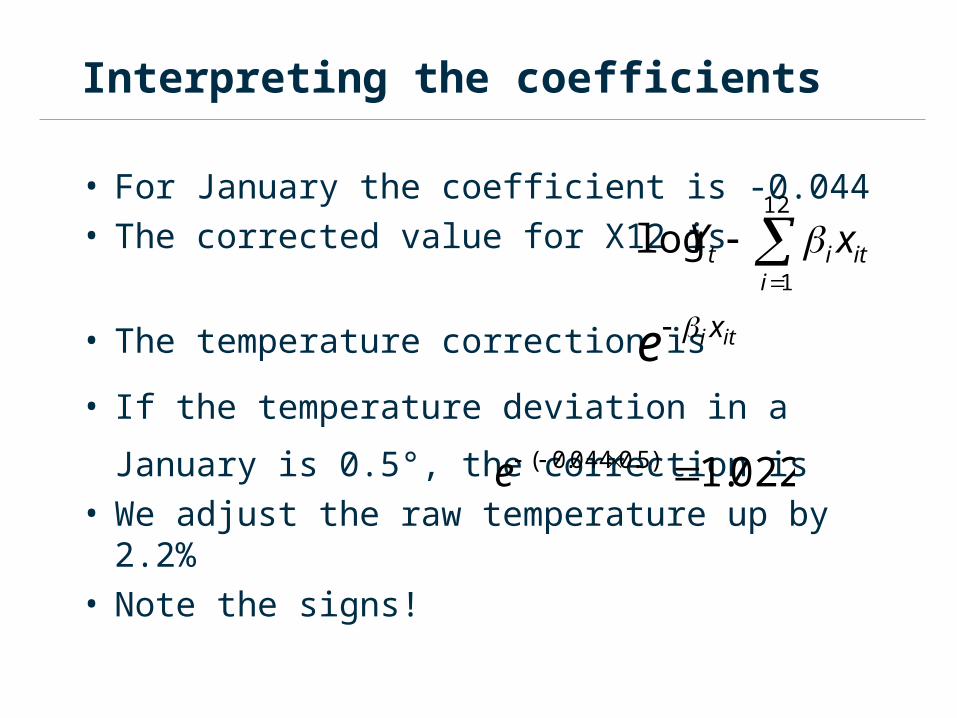
Interpreting the coefficients

• For January the coefficient is -0.044• The corrected value for X12 is

• The temperature correction is

• If the temperature deviation in a January is

0.5°, the correction is• We adjust the raw temperature up by 2.2%• Note the signs!

12

1

logi

itit xY

itixe

022.1)5.0044.0( e

Interpreting the coefficients

• If is small then

• So a negative coefficient is interpretable as a temperature correction factor as currently used by DECC

• Remember: a positive deviation leads to an upwards adjustment

itix xe iti 1

itix

Coal – estimated coefficients

-15

-10

-5

0

5

10

15

20


coef

fici

ent

(per

cen

tag

e)

Gas – estimated coefficients

0

2

4

6

8

10

12


co

eff

icie

nt

(pe

rce

nta

ge

)

Smoothing the coefficients for coal

Coefficients for coal

-15

-10

-5

0

5

10

15

20


co

eff

icie

nt

(%)

Coefficients for gas

0

2

4

6

8

10

12


coef

fici

ent

(%)

Comparing seasonal adjustments

Coal consumption, seasonally adjusted

3000

3500

4000

4500

5000

5500

6000

6500

7000

7500

8000

Jan-

95

Jul-9

5

Jan-

96

Jul-9

6

Jan-

97

Jul-9

7

Jan-

98

Jul-9

8

Jan-

99

Jul-9

9

Jan-

00

Jul-0

0

Jan-

01

Jul-0

1

Jan-

02

Jul-0

2

Jan-

03

Jul-0

3

Jan-

04

Jul-0

4

Jan-

05

Jul-0

5

Jan-

06

Jul-0

6

Jan-

07

Jul-0

7

Jan-

08

Jul-0

8

tho

usa

nd

s o

f to

nn

es

proposed new factors

current method of temperature correction

Heating degree days

• The difference between the maximum temperature in a day and some target temperature

• If the temperature in one day is above the target then the degree day measure is zero for that day

• The choice of target temperature is important

Smoothing the coefficients, heating degree days model (Eurostat measure)

Coefficients for coal

-0.20

-0.15

-0.10

-0.05

0.00

0.05

0.10

0.15

0.20


co

rre

cti

on

fa

cto

r, p

er

un

it d

ev

iati

on

fro

m t

he

a

ve

rag

e d

eg

ree

da

y

Coefficients for gas

0.00

0.02

0.04

0.06

0.08

0.10

0.12

0.14


corr

ecti

on

fac

tor,

per

un

it

dev

iati

on

fro

m t

he

aver

age

deg

ree

day

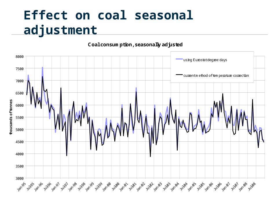
Effect on coal seasonal adjustment

Coal consumption, seasonally adjusted

3000

3500

4000

4500

5000

5500

6000

6500

7000

7500

8000

Jan-

95

Jul-9

5

Jan-

96

Jul-9

6

Jan-

97

Jul-9

7

Jan-

98

Jul-9

8

Jan-

99

Jul-9

9

Jan-

00

Jul-0

0

Jan-

01

Jul-0

1

Jan-

02

Jul-0

2

Jan-

03

Jul-0

3

Jan-

04

Jul-0

4

Jan-

05

Jul-0

5

Jan-

06

Jul-0

6

Jan-

07

Jul-0

7

Jan-

08

Jul-0

8

tho

usa

nd

s o

f to

nn

es

using Eurostat degree days

current method of temperature correction

The difference temperature correction can make!

Primary energy consumption

Million tonnes of oil equivalent

Unadjusted Temperature adjusted

2009 211.1 212.6

2010 217.3 211.3

Annual change +2.9% -0.6%

Documents

Temperature correction of energy consumption time series Sumit Rahman, Methodology Advisory Service, Office for National Statistics