Embed Size (px)
Citation preview

Research Collection
Doctoral Thesis
Microfluidic Thermoelectric Heat Exchangers for Low-Temperature Waste Heat Recovery
Author(s): Wojtas, Nina Z.
Publication Date: 2014
Permanent Link: https://doi.org/10.3929/ethz-a-010195663
Rights / License: In Copyright - Non-Commercial Use Permitted
This page was generated automatically upon download from the ETH Zurich Research Collection. For moreinformation please consult the Terms of use.
ETH Library
Diss. ETH No. 21783
Microfluidic Thermoelectric HeatExchangers for Low-Temperature
Waste Heat Recovery
A dissertation submitted to
ETH ZURICH
for the degree of
Doctor of Sciences
presented by
Nina Zuzanna WojtasMSc ETH Micro and Nanosystems
born October 03, 1982
citizen of Illnau-Effretikon ZH
accepted on the recommendation of
Prof. Dr. Christofer Hierold, examiner
Prof. Dr. Dimos Poulikakos, co-examiner
2014

ii

Document typeset by the author using the LATEX 2ε system and the KOMA-Scriptdocument class scrbook.
Copyright c© 2014 Nina Wojtas, Zürich


”Always do whatever’s next.”
- George Carlin
To my family –
v

Abstract
More than half of the energy created by humanity is lost as waste heat into theenvironment. Over 75 % of this dissipated energy is classified as low grade wasteheat and its temperature lies below 100 C. By recovering part of this waste en-ergy, the primary energy usage could be significantly reduced and thus the ecolo-gical footprint decreased. However, most technologies fail to produce electricalpower at these low temperature levels. A possible solution is offered by ther-moelectricity, where power can be generated starting from thermal gradients atarbitrary low temperatures.
There is a significant push to increase the output performance of thermoelec-tric generators (TEGs) in order to make them more competitive energy harvesters.The thermal coupling of TEGs has a major impact on the effective temperaturegradient across the generator and therefore the power output achieved. Thiswork reports on a novel approach combining efficient microfluidic thermal coup-ling and thin film generators in order to contribute to a significant thermoelectricoutput performance enhancement.The proposed thermoelectric heat exchanger (TEHEX) for low temperature wasteheat recovery consist of µTEGs in between multi-layer micro heat transfer sys-tems (µHTSs) featuring very low heat transfer resistances and small pumpingpowers. The implementation of efficient thermal coupling allows for the applic-ation of thin film generators for a thermally matched system and thus maximalpower output. Additionally, very compact systems and therefore high powerdensities can be achieved.
The TEHEXs are fabricated in two different size scales and characterized withrespect to their net output performance. By means of a small size 8 x 8 mm devicefeaturing high aspect ratio copper microchannels, the influence of the most rel-evant system parameters, i.e. the microchannel width, applied fluid flow ratesand the µTEG thickness on the system net output performance is investigated. Itis shown that dimensions of the µTEG and µHTS can be optimized for specifictemperature ranges applied, and the maximum net power can be tracked by ad-justing the heat transfer resistance during operation. With the compact system,a total of 63 mW/cm2 at a fluid inlet temperature difference of 60 K is measured.This corresponds to a net volumetric efficiency factor (VEF) of 37 W/m3K2, whichis by a factor of 4.8 higher than reported elsewhere. The fabricated 9 x 9 cm large
vii
TEHEX demonstrates the feasibility of a scalable low-cost technology and repres-ents a successful proof of concept for a commercial application in waste heat re-covery. The system characterization yields a net power of 0.44 W for one TEHEXunit at an applied fluid thermal gradient of 50 K, corresponding to a net VEF of5.1 W/m3K2 per active TEG area, also being the highest among reported net val-ues.With the characterized systems, the established 1D TEHEX model could be veri-fied and used as a powerful tool for further system analysis and optimizations.By optimizing the geometric parameters of the system as well as the operatingconditions, an output power enhancement of up to 65 % could be achieved at anapplied thermal gradient of 50 K.
viii
Zusammenfassung
Mehr als die Hälfte der von Menschen erzeugten Energie geht in Form von Ab-wärme verloren. Über 75 % dieser ungenutzten Energie wird als niedriggradigeAbwärme klassifiziert, da ihre Temperatur unterhalb von 100 C liegt. Durch eineteilweise Rückgewinnung dieser verlorenen Energie könnte der Primärenergie-verbrauch sowie der ökologische Fussabdruck signifikant reduziert werden. ImNiedertemperaturbereich versagen jedoch konventionelle Technologien der Ener-giegewinnung. Eine mögliche Lösung bietet die Thermoelektrizität, dank der be-reits bei beliebig kleinen Temperaturgradienten Energie erzeugt werden kann.
Es besteht ein grosses Interesse die Leistung von thermoelektrischen Genera-toren (TEG) zu steigern, um sie zu kompetitiveren Energiewandlern zu machen.Die thermische Ankopplung der TEG hat einen wesentlichen Einfluss auf den ef-fektiven Temperaturgradienten über dem Generator und dementsprechend aufdessen Ausgangsleistung. Im Rahmen dieser Arbeit wird ein neuartiges Konzeptentwickelt, welches eine effiziente thermische Ankopplung mittels Mikrofluidikmit Dünnschichtgeneratoren verbindet. Dieser Ansatz führt zu einer erheblichenthermoelektrischen Leistungssteigerung des Systems.Der vorgeschlagene Aufbau eines thermoelektrischen Wärmetauschers (TEHEX)für Abwärmerückgewinnung bei niedrigen Temperaturgradienten, besteht ausalternierend gestapelten µTEG und mehrschichtigen Mikrowärmeübertragungs-systemen (µHTS). Die entwickelten µHTS weisen sehr tiefe Wärmeübergangswi-derstände sowie eine kleine Pumpleistungen auf. Diese Implementierung der ef-fizienten thermischen Ankopplung erlaubt die Verwendung von Dünnschichtge-neratoren für thermisch abgeglichene Systeme, was zu einer Leistungsmaximie-rung führt. Zusätzlich können sehr kompakte Systeme mit hoher Leistungsdichteerreicht werden.
Die TEHEX werden in zwei verschiedenen Grössenordnungen hergestellt undbezüglich ihrer Nettoausgangsleistung charakterisiert. Mit dem kleinen 8 x 8 mmSystem, welches Mikrokupferkanäle mit hohem Aspektverhältnis aufweist, wer-den die Einflüsse der wichtigsten Systemparameter (i.e. Breite der Mikrokanäle,applizierte Durchflussrate sowie Dicke der Generatoren) auf den Nettoleistungs-ertrag untersucht. Es wird gezeigt, dass die Dimensionen der µTEG und µHTSfür spezifische Temperaturbereiche optimiert werden können und dass die ma-ximale Nettoleistung während dem Betrieb mittels Anpassung der Wärmeüber-
ix
gangswiderstände verfolgt werden kann. Mit dem kompakten System konnteeine Nettoleistung von 63 mW/cm2 bei einem angelegten Fluidtemperaturgra-dienten von 60 K gemessen werden. Dies entspricht einem netto Volumeneffizi-enzfaktor (VEF) von 37 W/m3K2 und ist damit 4.8 Mal höher als anderweitigberichtet. Der fabrizierte 9 x 9 cm grosse TEHEX demonstriert die Realisierbar-keit einer skalierbaren und kostengünstigen Technologie und liefert den Mach-barkeitsnachweis für eine kommerzielle Anwendung im Bereich der Abwärme-rückgewinnung. Die Charakterisierung des Systems ergibt bei einem angelegtenTemperaurgradienten von 50 K eine Nettoleistung von 0.44 W für eine TEHEX-Einheit. Dies entspricht einem netto VEF von 5.1 W/m3K2 pro aktive TEG Fläche,was ebenfalls einer der höchsten publizierten Nettowerte darstellt.Anhand der charakterisierten Systeme konnte das aufgestellte eindimensionaleModel des TEHEX validiert und als wichtiges Werkzeug für eine weiterführen-de Systemanalyse und Optimierung verwendet werden. Durch Optimierung dergeometrischen Systemparameter und der Betriebsbedingungen konnte eine theo-retische Leistungssteigerung von bis zu 65 % bei einem angelegten Temperatur-gradienten von 50 K aufgezeigt werden.
x
Contents
Abstract vii
Zusammenfassung ix
List of Symbols and Abbreviations xiii
1 Introduction 11.1 Rationale . . . . . . . . . . . . . . . . . . . . . . . . . . . . . . . . . . 11.2 Concept of compact TEHEX enabled by microfluidic coupling . . . 31.3 Objective and outline of this work . . . . . . . . . . . . . . . . . . . 5
2 State of the Art 72.1 Large size thermoelectric heat exchangers . . . . . . . . . . . . . . . 72.2 Thermoelectric generators in combination with microfluidics . . . . 12
3 Theory and Modelling 133.1 Thermoelectric generators . . . . . . . . . . . . . . . . . . . . . . . . 13
3.1.1 Fundamentals of thermoelectricity . . . . . . . . . . . . . . . 133.1.2 Thermoelectric materials and modules . . . . . . . . . . . . 153.1.3 Thermoelectric generator modelling . . . . . . . . . . . . . . 183.1.4 Impedance matching . . . . . . . . . . . . . . . . . . . . . . . 203.1.5 TEG model conclusions and considerations . . . . . . . . . . 23
3.2 Micro heat transfer system . . . . . . . . . . . . . . . . . . . . . . . . 283.2.1 Fluid dynamics in confined ducts . . . . . . . . . . . . . . . 283.2.2 Basic micro heat transfer system model . . . . . . . . . . . . 313.2.3 Model extensions . . . . . . . . . . . . . . . . . . . . . . . . . 353.2.4 3D FEM unit cell model . . . . . . . . . . . . . . . . . . . . . 39
3.3 Thermoelectric heat exchanger model . . . . . . . . . . . . . . . . . 433.4 Conclusions . . . . . . . . . . . . . . . . . . . . . . . . . . . . . . . . 44
4 Fabrication and Experimental 474.1 Thermoelectric heat exchanger fabrication . . . . . . . . . . . . . . . 47
4.1.1 Small size micro heat transfer system . . . . . . . . . . . . . 474.1.2 Large size micro heat transfer system . . . . . . . . . . . . . 54
4.2 Experimental . . . . . . . . . . . . . . . . . . . . . . . . . . . . . . . 584.2.1 Small size thermoelectric heat exchanger . . . . . . . . . . . 58
xi
Contents
4.2.2 Large size thermoelectric heat exchanger . . . . . . . . . . . 614.3 Conclusions . . . . . . . . . . . . . . . . . . . . . . . . . . . . . . . . 62
5 Device Characterisation 655.1 Small size thermoelectric heat exchanger . . . . . . . . . . . . . . . 65
5.1.1 Micro heat transfer system . . . . . . . . . . . . . . . . . . . 655.1.2 µHTS/µTEG system . . . . . . . . . . . . . . . . . . . . . . . 695.1.3 Thermoelectric heat exchanger . . . . . . . . . . . . . . . . . 76
5.2 Large size thermoelectric heat exchanger . . . . . . . . . . . . . . . 785.3 Conclusions . . . . . . . . . . . . . . . . . . . . . . . . . . . . . . . . 83
6 Thermoelectric Heat Exchanger Simulations 856.1 Simulation results . . . . . . . . . . . . . . . . . . . . . . . . . . . . . 85
6.1.1 Impact of individual parameters . . . . . . . . . . . . . . . . 856.1.2 System level optimization . . . . . . . . . . . . . . . . . . . . 886.1.3 Optimization routine . . . . . . . . . . . . . . . . . . . . . . . 90
6.2 Case study: marine propulsion engine . . . . . . . . . . . . . . . . . 936.2.1 Cost analysis . . . . . . . . . . . . . . . . . . . . . . . . . . . 94
6.3 Conclusions . . . . . . . . . . . . . . . . . . . . . . . . . . . . . . . . 95
7 Conclusion and Outlook 99
A Processing 103
B Measurement and Simulation Data 109
C GUI 121
Bibliography 125
Acknowledgement 141
Publications 143
Student Projects 145
Curriculum Vitae 147
xii
List of Symbols
Symbol Units Description
α V/K Relative Seebeck coefficient of thermocoupleαm V/K Absolute Seebeck coefficient of a materialA m2 Surface areaAV − Active to inactive TEG area ratiocp J/kgK Specific heat capacityCc − Constriction loss coefficientsCe − Expansion loss coefficientsdch m Characteristic channel lengthdhyd m Hydraulic diameterdTEG m Thermocouple diameterη − EfficiencyηC − Carnot efficiencyη2nd − Second order efficiencyf − Fanning friction factorφ V Electrical potentialhconv W/m2K Convective heat transfer coefficientI A Electrical currentκT V/K Thomson coefficientKcon cm2K/W Total contact thermal resistanceKHTS cm2K/W Thermal resistance of the heat transfer systemKTEG cm2K/W Thermal resistance of the generatorλ W/mK Thermal conductivity of TE materiall m Lengthlh m Hydrodynamic entrance lengthlTEG m Thermocouple lengthµ Pa s Dynamic viscositym − Number of thermocouplesNu − Nusselt numberΠ V Peltier coefficient∆p Pa Pressure dropPout W Output powerPout_net W Net output powerPF W/mK2 Power factor
xiii
Contents
PFm W/K2 Module power factorQ W Thermal fluxρel Ω m Electrical resistivityρc Ω m2 Specific contact resistivityρ f kg/m3 Density of the fluidRel Ω Electrical resistance of the generatorRe f f Ω Effective el. resistance of the generatorRl Ω Electrical load resistanceRe − Reynolds numbers m Distance between Thermocouplesσ S/m Electrical conductivityτxy − Normalized shear stresst m ThicknessT K TemperatureT K Average temperature∆T K Temperature difference∆TTEG K Temperature difference across the generator∆T0 K External temperature difference~∇T K Temperature gradientu m/s Fluid velocityV m3 System volumeVoc V Open circuit voltageVS V Seebeck voltageV m3/s Volumetric flow rateZ K−1 Material figure of meritZT − Dimensionless figure of meritZm K−1 Module figure of meritZTm − Dimensionless module figure of merit
xiv
Contents
Abbreviations
Abbreviation Description
1D One-dimensionalBCB BenzocyclobuteneCWC Cylinder water coolerDFR Dry film resistDI Distilled waterDOS Density of statesECD Electrochemical depositionFEM Finite element methodGBL γ-butyrolactoneGUI Graphical user interfaceHCL Hydrochloric acidHES Heat exchange systemHNO3 Nitric acidHTS Heat transfer systemIPA IsopropanolLOR Lift-Off resistMC MicrochannelMF ManifoldPF Power factorPMMA Poly(methyl methacrylate)TC ThermocoupleTE ThermoelectricTEG Thermoelectric generatorTEHEX Thermoelectric heat exchangerUS UltrasoundUV UltravioletVEF Volumetric efficiency factorWHR Waste heat recoveryWLI White light interferometry
xv

1 Introduction
The simultaneous rise in energy consumption and environmental awareness cre-ates a worldwide growing demand for more efficient and clean energy systems.One promising approach to improve a system’s efficiency is to reduce the thermallosses by recovering a part of the produced waste heat. At least half of the energycreated by humanity is dissipated as waste heat into the environment [1, 2]. Con-temporary vehicle engines, for example, lose more than 60 % of their fuel energyin the form of heat [3]. Also most of today’s steam generator based electricalpower plants run on a very low average net efficiency below 36 %, and are there-fore creating enormous amounts of waste heat [2, 4]. Thus, with the perspectiveof reducing primary energy usage and decreasing environmental impacts, theinterest in waste heat recovery has gained more and more attention [2, 5, 6]. Apotential correlation between global warming and produced waste heat has evenbeen discussed [7, 8].Apart from established technologies to convert waste heat into electricity bymeans of combined turbine cycles or recuperative heating [2], thermoelectricityhas been identified as a promising approach to recover energy [9–11]. Thermo-electric generators (TEGs) convert an applied thermal gradient directly into elec-trical energy by taking advantage of the Seebeck effect. Although thermoelectricpower generation cannot compete with the existing thermodynamic cycles withrespect to conversion efficiency [12], it offers several other advantages such asdevice simplicity, compactness, scalability and an arbitrarily low operating tem-perature range. The last point is of particular importance, since most of the wasteheat is available in the range below 100 C [2], where other technologies fail toproduce electrical power. Therefore, the most attractive applications for thermo-electric power generation lie in low temperature waste heat recovery from tech-nical or natural sources [9, 11, 13, 14], transportation [15, 16] as well as energyharvesting for small autonomous systems [17–19].
1.1 Rationale
So far, the commercial applications of TEGs have been limited to niche marketssuch as aerospace [20, 21] and power supply in remote or hazardous places[22, 23]. The main reasons for this are (1) the relatively low thermoelectricconversion efficiency, (2) high fabrication costs of thermoelectric modules, (3)suboptimal exploitation of the available temperature gradients and (4) neglecting
1
1 Introduction
the importance of a thorough system level optimization. While much effortis spent to improve the thermoelectric figure of merit ZT by nanostructuring[24–26] as well as to develop low-cost fabrication technologies [27–29], less atten-tion has been paid to maximizing the thermal gradient exploitation and systemlevel optimization. This in particular relates to the thermal coupling of thethermoelectric device to the heat source and the heat sink, an optimal matchingof the thermal contact and TEG resistances [30], as well as the consideration ofthe net system performance.
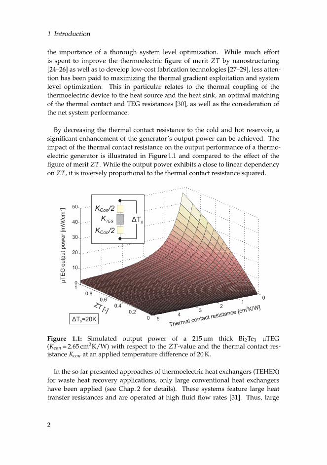
By decreasing the thermal contact resistance to the cold and hot reservoir, asignificant enhancement of the generator’s output power can be achieved. Theimpact of the thermal contact resistance on the output performance of a thermo-electric generator is illustrated in Figure 1.1 and compared to the effect of thefigure of merit ZT. While the output power exhibits a close to linear dependencyon ZT, it is inversely proportional to the thermal contact resistance squared.
0
0.2
0.4
0.6
0.8
1
01
23
45
0
10
20
30
40
50
2]
ΔT =20K0
mT
EG
ou
tpu
t p
ow
er
[mW
/cm
ZT [-]
Thermal contact resistance [cm K/W]2
KTEG ΔT0
K /2Con
K /2Con
Figure 1.1: Simulated output power of a 215µm thick Bi2Te3 µTEG(Kcon = 2.65 cm2K/W) with respect to the ZT-value and the thermal contact res-istance Kcon at an applied temperature difference of 20 K.
In the so far presented approaches of thermoelectric heat exchangers (TEHEX)for waste heat recovery applications, only large conventional heat exchangershave been applied (see Chap. 2 for details). These systems feature large heattransfer resistances and are operated at high fluid flow rates [31]. Thus, large
2
1.2 Concept of compact TEHEX enabled by microfluidic coupling
pumping powers are needed, which are mostly neglected in the overall systemscharacterization.
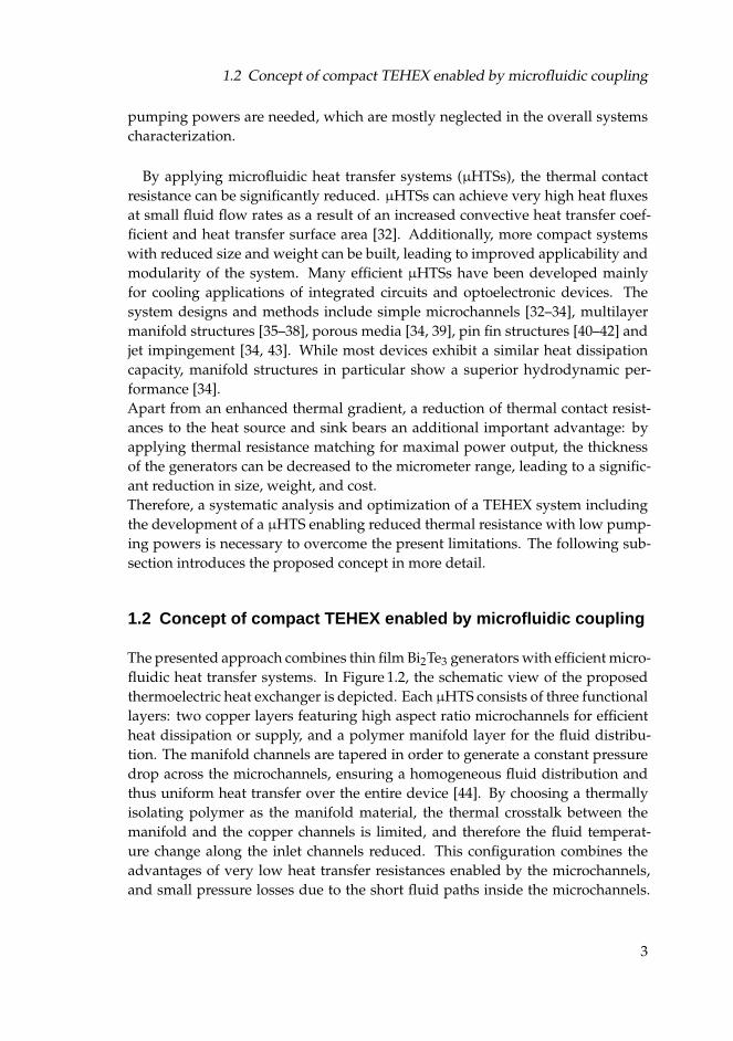
By applying microfluidic heat transfer systems (µHTSs), the thermal contactresistance can be significantly reduced. µHTSs can achieve very high heat fluxesat small fluid flow rates as a result of an increased convective heat transfer coef-ficient and heat transfer surface area [32]. Additionally, more compact systemswith reduced size and weight can be built, leading to improved applicability andmodularity of the system. Many efficient µHTSs have been developed mainlyfor cooling applications of integrated circuits and optoelectronic devices. Thesystem designs and methods include simple microchannels [32–34], multilayermanifold structures [35–38], porous media [34, 39], pin fin structures [40–42] andjet impingement [34, 43]. While most devices exhibit a similar heat dissipationcapacity, manifold structures in particular show a superior hydrodynamic per-formance [34].Apart from an enhanced thermal gradient, a reduction of thermal contact resist-ances to the heat source and sink bears an additional important advantage: byapplying thermal resistance matching for maximal power output, the thicknessof the generators can be decreased to the micrometer range, leading to a signific-ant reduction in size, weight, and cost.Therefore, a systematic analysis and optimization of a TEHEX system includingthe development of a µHTS enabling reduced thermal resistance with low pump-ing powers is necessary to overcome the present limitations. The following sub-section introduces the proposed concept in more detail.
1.2 Concept of compact TEHEX enabled by microfluidic coupling
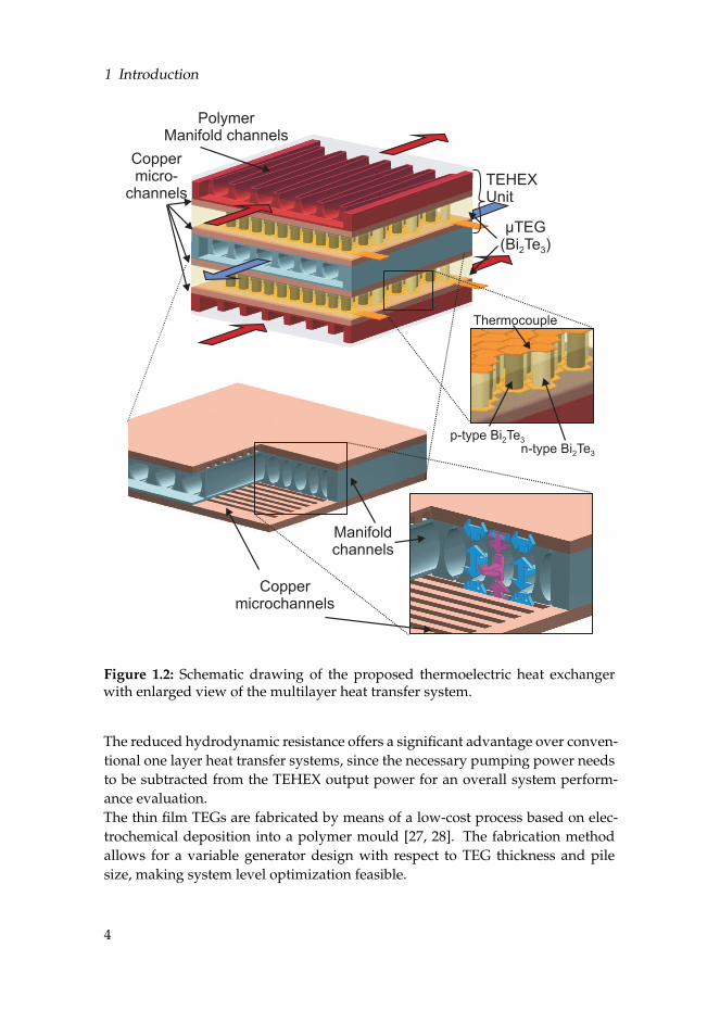
The presented approach combines thin film Bi2Te3 generators with efficient micro-fluidic heat transfer systems. In Figure 1.2, the schematic view of the proposedthermoelectric heat exchanger is depicted. Each µHTS consists of three functionallayers: two copper layers featuring high aspect ratio microchannels for efficientheat dissipation or supply, and a polymer manifold layer for the fluid distribu-tion. The manifold channels are tapered in order to generate a constant pressuredrop across the microchannels, ensuring a homogeneous fluid distribution andthus uniform heat transfer over the entire device [44]. By choosing a thermallyisolating polymer as the manifold material, the thermal crosstalk between themanifold and the copper channels is limited, and therefore the fluid temperat-ure change along the inlet channels reduced. This configuration combines theadvantages of very low heat transfer resistances enabled by the microchannels,and small pressure losses due to the short fluid paths inside the microchannels.
3
1 Introduction
PolymerManifold channels
µTEG(Bi Te )2 3
TEHEXUnit
Manifoldchannels
n-type Bi Te2 3
p-type Bi Te2 3
Coppermicrochannels
Coppermicro-
channels
Thermocouple
Figure 1.2: Schematic drawing of the proposed thermoelectric heat exchangerwith enlarged view of the multilayer heat transfer system.
The reduced hydrodynamic resistance offers a significant advantage over conven-tional one layer heat transfer systems, since the necessary pumping power needsto be subtracted from the TEHEX output power for an overall system perform-ance evaluation.The thin film TEGs are fabricated by means of a low-cost process based on elec-trochemical deposition into a polymer mould [27, 28]. The fabrication methodallows for a variable generator design with respect to TEG thickness and pilesize, making system level optimization feasible.
4
1.3 Objective and outline of this work
1.3 Objective and outline of this work
Based on the proposed compact stacked thermoelectric heat exchanger system,the following objectives are pursued within the framework of this thesis:
1. Investigation of the impact of microscopic features on the system level per-formance of macroscopic thermoelectric heat exchangers. The objectiveis to show how the combination of optimized microfluidic concepts andmatched thin film generators will enhance the net performance of TEHEXs.
2. Development of suitable fabrication processes for the implementation ofhighly efficient micro heat transfer systems on two different size scales:one small size approach to investigate the different parameter dependen-cies and achievable net system performance, and a large size approach toshow the feasibility of a scalable low-cost technology as well as to demon-strate the potential for low temperature waste heat recovery. The focus isset on the technology developed for high aspect ratio microchannels andon the implementation of optimal material combinations.
3. A systematic analysis, characterization and modelling of the TEHEX in or-der to investigate the most important system parameters and to allow for aprofound system understanding and model validation.
4. Application of the verified model for a detailed optimization study, as wellas the demonstration of the systems potential and technological limitationswith respect to specific applications in low temperature waste heat recov-ery.
The thesis is structured as fallows:
In Chapter 2, the state of the art of existing liquid-liquid and gas-liquid thermo-electric heat exchangers is discussed and compared by means of an introducedsystem comparison factor, the volumetric efficiency factor (VEF). Further, firstsystems of thermoelectric generators combined with microfluidic approaches arereviewed.
In Chapter 3, the theory and model of the two main components of the ther-moelectric heat exchanger, the TEG and the µHTS, are introduced and discussedseparately. Important design aspects and parameter interdependencies are high-lighted and fist system improvements are proposed. The final combined TEHEXmodel is presented and the computation routine is outlined.
5
1 Introduction
In Chapter 4, the developed fabrication process of the small and large sizeµHTS is documented and the advantages and limitations of the applied techno-logies are discussed. Furthermore, the assemblies of the two TEHEXs, the corres-ponding measurement setups and measurement conditions are explained.
In Chapter 5, the fabricated small and large size TEHEXs are characterizedand the impact of different design parameters and boundary conditions on thenet performance is investigated. The characterization results are compared to the1D model developed in parallel, and related to the current state of the art.
In Chapter 6, the verified model is used for a systematic analysis of the mostimportant TEHEX design parameters and for a system level optimization. Ad-ditionally, the performance and profitability of the optimized system design isestimated for the specific application in a marine propulsion engine.
In Chapter 7, the most important results are summarized and correspondingconclusions are drawn. Further, a brief outlook is given in perspective of poten-tial applications.
6
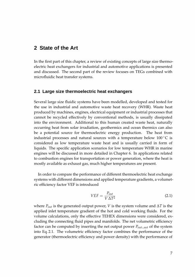
2 State of the Art
In the first part of this chapter, a review of existing concepts of large size thermo-electric heat exchangers for industrial and automotive applications is presentedand discussed. The second part of the review focuses on TEGs combined withmicrofluidic heat transfer systems.
2.1 Large size thermoelectric heat exchangers
Several large size fluidic systems have been modelled, developed and tested forthe use in industrial and automotive waste heat recovery (WHR). Waste heatproduced by machines, engines, electrical equipment or industrial processes thatcannot be recycled effectively by conventional methods, is usually dissipatedinto the environment. Additional to this human created waste heat, naturallyoccurring heat from solar irradiation, geothermics and ocean thermics can alsobe a potential source for thermoelectric energy production. The heat fromindustrial processes and natural sources with a temperature below 100 C isconsidered as low temperature waste heat and is usually carried in form ofliquids. The specific application scenarios for low temperature WHR in marineengines will be discussed in more detailed in Chapter 6. In applications relatedto combustion engines for transportation or power generation, where the heat ismostly available as exhaust gas, much higher temperatures are present.
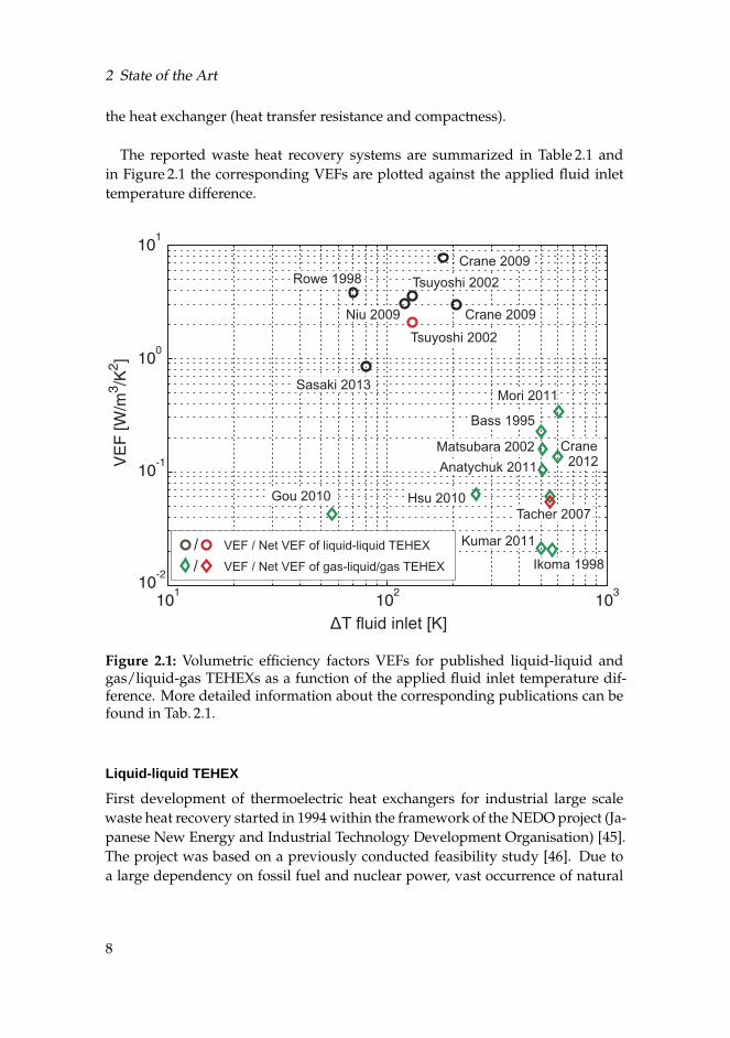
In order to compare the performance of different thermoelectric heat exchangesystems with different dimensions and applied temperature gradients, a volumet-ric efficiency factor VEF is introduced
VEF =Pout
V ∆T2 (2.1)
where Pout is the generated output power, V is the system volume and ∆T is theapplied inlet temperature gradient of the hot and cold working fluids. For thevolume calculations, only the effective TEHEX dimensions were considered, ex-cluding the connecting fluid pipes and manifolds. The net volumetric efficiencyfactor can be computed by inserting the net output power Pout_net of the systeminto Eq. 2.1. The volumetric efficiency factor combines the performance of thegenerator (thermoelectric efficiency and power density) with the performance of
7
2 State of the Art
the heat exchanger (heat transfer resistance and compactness).
The reported waste heat recovery systems are summarized in Table 2.1 andin Figure 2.1 the corresponding VEFs are plotted against the applied fluid inlettemperature difference.
Rowe 1998
Crane 2009
Tsuyoshi 2002
Niu 2009 Crane 2009
Tsuyoshi 2002
Sasaki 2013
Gou 2010 Hsu 2010
Bass 1995
Matsubara 2002 Crane2012
Tacher 2007
Kumar 2011
Ikoma 1998
Mori 2011
Anatychuk 2011
VEF / Net VEF of liquid-liquid TEHEX
VEF / Net VEF of gas-liquid/gas TEHEX
/
/
ΔT fluid inlet [K]
Figure 2.1: Volumetric efficiency factors VEFs for published liquid-liquid andgas/liquid-gas TEHEXs as a function of the applied fluid inlet temperature dif-ference. More detailed information about the corresponding publications can befound in Tab. 2.1.
Liquid-liquid TEHEX
First development of thermoelectric heat exchangers for industrial large scalewaste heat recovery started in 1994 within the framework of the NEDO project (Ja-panese New Energy and Industrial Technology Development Organisation) [45].The project was based on a previously conducted feasibility study [46]. Due toa large dependency on fossil fuel and nuclear power, vast occurrence of natural
8
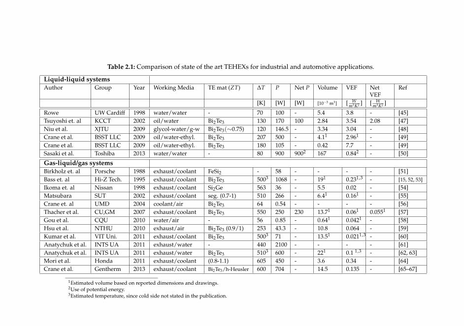
Table 2.1: Comparison of state of the art TEHEXs for industrial and automotive applications.
Liquid-liquid systems
Author Group Year Working Media TE mat (ZT) ∆T P Net P Volume VEF NetVEF
Ref
[K] [W] [W] [10−3 m3] [ Wm3K2 ] [ W
m3K2 ]
Rowe UW Cardiff 1998 water/water - 70 100 - 5.4 3.8 - [45]Tsuyoshi et. al KCCT 2002 oil/water Bi2Te3 130 170 100 2.84 3.54 2.08 [47]Niu et al. XJTU 2009 glycol-water/g-w Bi2Te3(∼0.75) 120 146.5 - 3.34 3.04 - [48]Crane et al. BSST LLC 2009 oil/water-ethyl. Bi2Te3 207 500 - 4.11 2.961 - [49]Crane et al. BSST LLC 2009 oil/water-ethyl. Bi2Te3 180 105 - 0.42 7.7 - [49]Sasaki et al. Toshiba 2013 water/water - 80 900 9002 167 0.842 - [50]
Gas-liquid/gas systems
Birkholz et. al Porsche 1988 exhaust/coolant FeSi2 - 58 - - - - [51]Bass et. al Hi-Z Tech. 1995 exhaust/coolant Bi2Te3 5003 1068 - 191 0.231,3 - [15, 52, 53]
Ikoma et. al Nissan 1998 exhaust/coolant Si2Ge 563 36 - 5.5 0.02 - [54]Matsubara SUT 2002 exhaust/coolant seg. (0.7-1) 510 266 - 6.41 0.161 - [55]Crane et. al UMD 2004 coolant/air Bi2Te3 64 0.54 - - - - [56]Thacher et al. CU,GM 2007 exhaust/coolant Bi2Te3 550 250 230 13.71 0.061 0.0551 [57]Gou et al. CQU 2010 water/air - 56 0.85 - 0.641 0.0421 - [58]Hsu et al. NTHU 2010 exhaust/air Bi2Te3 (0.9/1) 253 43.3 - 10.8 0.064 - [59]Kumar et al. VIT Uni. 2011 exhaust/coolant Bi2Te3 5003 71 - 13.51 0.0211,3 - [60]Anatychuk et al. INTS UA 2011 exhaust/water - 440 2100 - - - - [61]Anatychuk et al. INTS UA 2011 exhaust/water Bi2Te3 5103 600 - 221 0.1 1,3 - [62, 63]Mori et al. Honda 2011 exhaust/coolant (0.8-1.1) 605 450 - 3.6 0.34 - [64]Crane et al. Gentherm 2013 exhaust/coolant Bi2Te3/h-Heusler 600 704 - 14.5 0.135 - [65–67]
1Estimated volume based on reported dimensions and drawings.2Use of potential energy.3Estimated temperature, since cold side not stated in the publication.

2 State of the Art
hot springs and strong environmental awareness, Japan has been proactive inthe development of new energy sources in perspective of future micro gridpower supply systems [68]. In the course of the project, high power densitymodules with smaller thermocouples and reduced spacing have been producedand integrated into fluidic heat exchangers. The developed WATT (Waste heatAlternative Thermoelectric Technology) modules were capable of delivering upto 100 W power at an applied fluid temperature difference of 80 K, reaching apower density of 18.5 kW/m3 [45]. A cost analysis of the system yielded a payback time of approximately two years.In 2005, a TEHEX employing 329 Bi2Te3 modules was installed at the Kusatsuhot springs, where a constant hot water supply at 369 K is available [14]. By2009, the plant generated more than 1360 kWh and was used for powering TVdisplays and lighting units. Tsuyoshi and Matsuura [47] reported modellingand experimental results of a thermoelectric engine composed of TEGs stackedbetween parallel plate heat exchangers using oil and water as active media. Atan applied temperature gradient of 130 K, an output power of 170 W total and100 W net could be reached. Niu et al. [48] built a similar parallel plate heatexchanger with commercially available Bi2Te3 modules, reaching 140 W at aninlet temperature difference of 120 K. Crane et al. [49] constructed a TEG - heatexchange assembly with a stack of 6 TEG modules producing 500 W at aninlet temperature difference of 205 K. A second generation high-power-densitysystem reached a VEF of 7.7, mainly due to the increase of the thermopile density.Toshiba [50] built and installed a thermoelectric plant that runs by the thermalenergy of natural hot spring water, reaching 900 W peak power (∆T = 80 K). Thegained energy was used to power LED lights in a hotel lobby. Commissionedin 2011, it has generated a total energy of 1927 kWh after a operating time of1.5 years. The water system was run by a potential energy difference, thus nopumping power was required.
Although the achieved output power values from the reported experimentalstudies are remarkable, the systems are very large and heavy, resulting in a max-imal VEF of 7.7 (see Fig. 2.1). In most cases, thick commercially available TEGsand standard large size heat exchangers are applied, where high amounts ofthe working fluid are pumped through the system and the consumed pumpingpower is neglected. Furthermore, the reported systems work without an optim-ized thermal contact resistance as well as overall system design.
Gas-liquid/gas TEHEX
Due to low conversion efficiencies of internal combustion engines (30 - 43 % [69])as well as the high energy consumption in the transportation sector, automotive
10
engines are predestined for thermal waste heat recovery. With the exhausttemperatures ranging from 500-1200 K and the cooling cycle temperature below350 K, high thermal gradients and moving fluids are available.
As early as 1914, the possibility of scavenging energy from the car exhaust hasbeen investigated [70] and a first prototype was built in 1964 [71]. In 1988, a ther-moelectric generator using 90 FeSi2 thermoelements was installed in a Porsche944 engine and delivered up to 58 W at full power [51]. Starting form 1991, Hi-ZTechnology Inc. started developing a thermoelectric recovery system for heavyduty trucks, reaching over 1 kW power on a test engine [15, 52, 53]. In the lastdecade, the interest in thermoelectric waste heat recovery in passenger cars hasexploded and an international workshop was dedicated exclusively to this topic[72]. All the main car companies inducing General Motors [57, 73], BMW [65–67, 74] or Toyota [55] are involved in thermoelectric projects. The best perform-ing TEHEX for passenger vehicles has been developed within the framework ofa seven-year program started in 2004, in a collaboration between Amerigon (nowGentherm), BMW and Ford. The result was a system integrated into a BMW X6and a Lincoln MKT reaching over 700 W on the test bench and over 600 W in on-vehicle tests (BMW). A net fuel efficiency increase of 1.2 % was reported [65–67].Not only vehicle exhaust gas, but also car radiators [56] or stationary dieselpower plants [61] have been identified as potential fields for thermoelectric heatexchange applications. In the latter example, up to 2.1 kW could be recovered,corresponding to 4.4 % of the total electric power produced by the diesel plant.
Despite the large development efforts towards automotive waste heat re-covery, several challenges need to be solved in order to enable a commercialbreakthrough of the technology. Next to reliability and long-term durabilityissues triggered by frequent thermal cycling, as well as the induced weightpenalty, the cost efficiency has been identified as the most critical criterion. Tomeet market requirements and be competitive with other emerging technologies,it is estimated that TE modules must be produced and assembled at a fraction oftoday’s cost [75]. To enhance the output power per cost, new fabrication techno-logies, higher ZT materials and optimization at the system level will be necessary.
Analogous to the liquid-liquid TEHEXs, the existing solutions work with thickand heavy commercial modules and do not take thermal optimization aspectsinto consideration. The calculated and estimated VEFs of the reported gas-liquidsystems are significantly lower compared to the liquid solutions. This is mainlydue to a lower thermal conductivity and heat capacity of the gases, i.e. lower heattransfer coefficients, as well as important dimensional constrains related to backpressure issues of the engine exhaust pipe.
2 State of the Art
2.2 Thermoelectric generators in combination with microfluidics
Although the importance of reduced thermal coupling resistances and systemlevel optimization has been identified and confirmed by simulations [30, 76–78],only few groups have started experimental investigations towards the integra-tion of TEGs with microfluidic heat transfer systems.
Reziana et al. simulated [79, 80] and published first experimental results [81] ofTEGs cooled by a parallel microchannel heat sink. The focus of the experimentalstudy was to explore the optimum coolant flow rate for a maximal net powerperformance of the system. With a setup consisting of a heater, a 56 x 56 mmTEG (G2-56-0375, Tellurex) and twenty plate-fin aluminium microchannelshaving a hydraulic diameter of 0.93 mm and an aspect ratio of approximately1, a maximal net power of 2 W was generated at a temperature difference of80 K directly across the TEG. The author concluded that the optimal coolantflow rate increases with increasing applied temperature gradient. Due to thesimple parallel microchannel structure, large pressure losses and a decrease ofthe thermal gradient along the channel flow would limit the device performancein a scaled up system.An interesting theoretical and experimental study of a phase change MEMS-based capillary heat exchanger designed as a heat sink for thermoelectric wasteenergy harvesting has been published by Mathew et al. [82]. The fabricatedprototypes consisted of silicon and SU-8 based heat exchangers with rectangular100µm wide and up to 375µm high microchannels (total footprint of 38 x 13 mm).A minimal thermal contact resistance of 33 m2K/W was reached operating at theboiling point of the working fluid.
Concluding from the discussed experimental works, the possible approachesfor improving the integration of microfluidic features mainly involve a systemdesign enabling efficient and homogeneous fluid distribution with low pumpingpower as well as smaller microchannels. Additionally, a sufficient heat capacityand corresponding flow rates of the working fluid must be achieved in order toallow efficient heat transfer.
12
3 Theory and Modelling
The first part of this chapter will introduce the fundamentals of thermoelectricityand TE modelling, as well as highlight important aspects and conclusions relatedto the module design and application. In the second part, theory and modellingof microfluidic heat transfer systems will be discussed. The final part will com-bine both fields and introduce the thermoelectric heat exchanger model.
3.1 Thermoelectric generators
3.1.1 Fundamentals of thermoelectricity
Three thermoelectric effects, the Seebeck [83], the Peltier and the Thomson effect,contribute to the direct conversion of heat into electricity and vice-versa. Theyare based on the interaction between heat and charge carriers and are thermody-namically reversible.
Seebeck effect
When a temperature gradient is applied to a conductor or semiconductor, an elec-tromotive force is generated, leading to the build up of electrical potential ~∇φ
~∇φ = −αm(T)~∇T (3.1)
where αm(T) is the absolute temperature dependent Seebeck coefficient and ~∇T
is the temperature gradient. For small temperature differences applied, αm can beassumed constant and the integration over the material will yield an expressionfor the generated Seebeck voltage
VS = −αm (Th − Tc) = −αm ∆T (3.2)
where Th and Tc are the applied temperatures at the hot and cold side of thematerial, respectively. In practice, the Seebeck voltage can only be exploited bycombining two materials with different (preferably opposite signed) Seebeck coef-ficients
VS1_2 = (αm1 − αm2) (Th − Tc) = α ∆T (3.3)
where α is the relative Seebeck coefficient of a thermocouple (TC). Applying thesame material would results in the cancellation of the electric potential.
13
3 Theory and Modelling
The Seebeck effect is based on the combination of several physical phenomenawhich will be briefly discussed [84]. The main contribution to the Seebeck effectin semiconductors is thermodiffusion [85]. The kinetic energy of the chargecarriers is temperature dependent. Therefore, the charge carriers on the hotside (electrons for n-type and holes for p-type semiconductors) have a higherkinetic energy and thus higher local thermal velocity than the carriers on thecold side. As a result, more carriers diffuse in average from the hot to thecold side than vice-versa, causing a charge accumulation at the cold end. Thecarrier concentration of semiconductors also strongly varies with temperature.A thermal gradient results in a carrier concentration gradient and thereforegradient based diffusion towards lower concentrations (cold side). Changes ofthe band gap with temperature can also lead to a carrier flow between the twoends of the semiconductor. In metals and semiconductors with approximatelyequal concentration of holes and electrons, the dependence of the diffusioncoefficient or the charge carrier mobility on temperature can lead to negativeas well as positive Seebeck coefficients. The Fermi level also reduces withincreasing temperature, resulting in an carrier movement from the cold to thehot side. Additionally, phonons follow the temperature gradient from the hotto the cold end. Due to phonon-charge carriers interactions, the carriers can bepushed along with the lattice vibrations by the so called phonon drag effect. Thecombination of all those effect leads to a final charge accumulation at either endof the conductor. The resulting electric field counteracts a further charge buildup and an equilibrium is reached.
Several approaches to physically model the Seebeck coefficient with differentlevels of complexities have been reported in literature [84, 86–88].
Peltier effect
When an electric current is flowing through a junction of two conducting ma-terials, heat is generated or absorbed. This heat current QP originates from thePeltier effect
QP = (Πm1 − Πm2) I = Π I = α T I (3.4)
where Πm is the absolute Peltier coefficient of one material, Π is the relative coef-ficient of the two conductors (i.e. the TC) and I is the electric current. The firstThomson relation links the Peltier with the Seebeck effect. In thermoelectric gen-erators, the Peltier heat is supplied by the hot side heat source and delivers theenergy for the electric current to run [89] .
14
3.1 Thermoelectric generators
Thomson effect
When an electric current is flowing through a homogeneous conductor with anapplied thermal gradient, heat is generated or absorbed (additional to the Jouleheat). This Thomson heat originates from the temperature dependent Seebeckcoefficient. If a current is driven through a conductor with an applied thermalgradient, a continuous Peltier effect will occur. The Thomson heat can be ex-pressed as
QT = κT I ∆T =dα
dTT I ∆T (3.5)
where κT is the Thomson coefficient. The second Thomson relation links the See-beck with the Thomson effect. Since the Thomson effect is small in comparisonto the other two thermoelectric effects, it is often neglected in the device mod-elling. Especially for small temperature gradients and thin-film TEGs, this is areasonable model simplification.
3.1.2 Thermoelectric materials and modules
The suitability of a material for thermoelectric conversion can be expressed withthe figure of merit [90]
Z =α2 σel
λ=
α2
λ ρel(3.6)
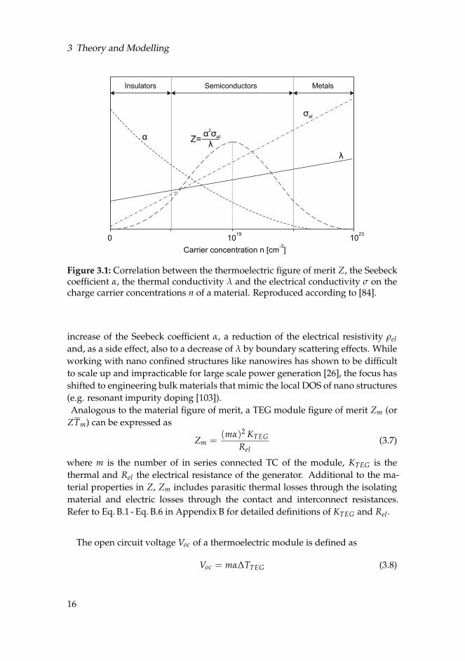
where λ is the thermal conductivity, σel is the electrical conductivity and ρel isthe electrical resistivity of the material. For efficient energy conversion, a lowthermal conductivity for high temperature gradients and low electrical resistiv-ity for low ohmic losses are desired. All three parameters of Z depend on thecharge carrier concentrations of the material (see Fig. 3.1). Therefore, an optimalcarrier concentration for high Z-values can be found between 1018 and 1020cm−3,corresponding to highly doped semiconductors and semi-metals.
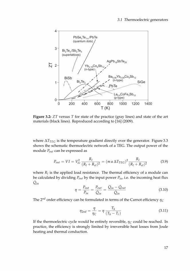
The more commonly used dimensionless figure of merit ZT is obtained bymultiplication with the average system temperature T. Figure 3.2 gives an over-view of the state of the art and state of the practice thermoelectric materialsand their ZT values. Next to the well established compound semiconductors(e.g. PbTe, Bi2Te3) with a maximum ZT around unity, new engineered materialshave emerged in the recent decade. This boost of ZT has been achieved through(1) enhancement of the electron density of states (DOS) near the Fermi level byquantum confinement or band gap engineering [91–96] and (2) an enhancementof phonon scattering by increasing the presence of interfaces [24, 25, 97–102] (e.g.grain boundaries, defects, dislocations, or acoustic mismatch). The latter can sig-nificantly reduce the phonon mean free path and thus the thermal conductivityλ of the TE material. Quantum confinement potentially leads to a simultaneous
15
3 Theory and Modelling
Insulators Semiconductors Metals
α
0 1019
1023
λ
α σ2
elZ=
Carrier concentration n [cm-3]
λ
σel
Figure 3.1: Correlation between the thermoelectric figure of merit Z, the Seebeckcoefficient α, the thermal conductivity λ and the electrical conductivity σ on thecharge carrier concentrations n of a material. Reproduced according to [84].
increase of the Seebeck coefficient α, a reduction of the electrical resistivity ρel
and, as a side effect, also to a decrease of λ by boundary scattering effects. Whileworking with nano confined structures like nanowires has shown to be difficultto scale up and impracticable for large scale power generation [26], the focus hasshifted to engineering bulk materials that mimic the local DOS of nano structures(e.g. resonant impurity doping [103]).Analogous to the material figure of merit, a TEG module figure of merit Zm (or
ZTm) can be expressed as
Zm =(mα)2 KTEG
Rel(3.7)
where m is the number of in series connected TC of the module, KTEG is thethermal and Rel the electrical resistance of the generator. Additional to the ma-terial properties in Z, Zm includes parasitic thermal losses through the isolatingmaterial and electric losses through the contact and interconnect resistances.Refer to Eq. B.1 - Eq. B.6 in Appendix B for detailed definitions of KTEG and Rel .
The open circuit voltage Voc of a thermoelectric module is defined as
Voc = mα∆TTEG (3.8)
16
3.1 Thermoelectric generators
1
3
4
2
00 200 400 600 800 1000 1200 1400
BiSbBi Te2 3
Bi Te /Sb Te2 3 2 3
(superlattices)
(quantum dots)
PbSe Te /PbTex 1-x
AgPb SbTe18 20
Ba Yb Co Sb0.08 0.09 4 12
Yb Co Sb0.19 4 12
(n-type)
(n-type)
La CoFe Sb0.9 3 12
(p-type)
PbTeSiGe
T (K)
ZT
Figure 3.2: ZT versus T for state of the practice (gray lines) and state of the artmaterials (black lines). Reproduced according to [16] (2009).
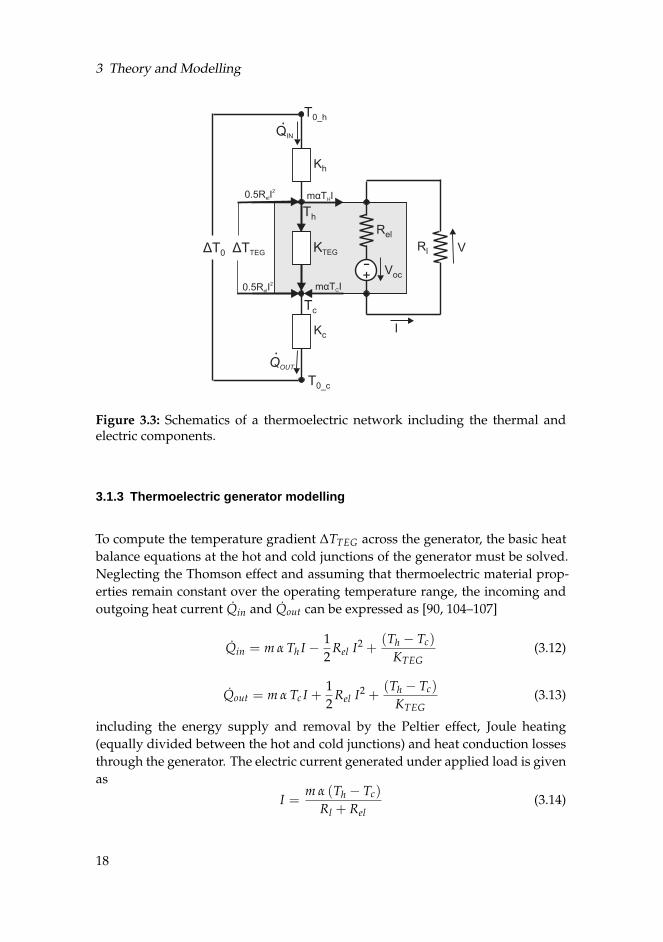
where ∆TTEG is the temperature gradient directly over the generator. Figure 3.3shows the schematic thermoelectric network of a TEG. The output power of themodule Pout can be expressed as
Pout = VI = V2oc
Rl
(Rl + Rel)2 = (m α ∆TTEG)2 Rl
(Rl + Rel)2 (3.9)
where Rl is the applied load resistance. The thermal efficiency of a module canbe calculated by dividing Pout by the input power Pin, i.e. the incoming heat fluxQin
η =Pout
Pin=
Pout
Qin
=Qin − Qout
Qin
(3.10)
The 2nd order efficiency can be formulated in terms of the Carnot efficiency ηC
η2nd =η
ηC= η
Th
(Th − Tc)(3.11)
If the thermoelectric cycle would be entirely reversible, ηC could be reached. Inpractice, the efficiency is strongly limited by irreversible heat losses from Jouleheating and thermal conduction.
17
3 Theory and Modelling
T0_h
ΔT0
Kh
QIN
QOUT
Kc
KTEG
T0_c
Th
Tc
ΔTTEGRl
Rel
ɠ+ Voc
I
V
mαTCI
mαTHI
0.5RelI2
0.5RelI2
Figure 3.3: Schematics of a thermoelectric network including the thermal andelectric components.
3.1.3 Thermoelectric generator modelling
To compute the temperature gradient ∆TTEG across the generator, the basic heatbalance equations at the hot and cold junctions of the generator must be solved.Neglecting the Thomson effect and assuming that thermoelectric material prop-erties remain constant over the operating temperature range, the incoming andoutgoing heat current Qin and Qout can be expressed as [90, 104–107]
Qin = m α Th I − 12
Rel I2 +(Th − Tc)
KTEG(3.12)
Qout = m α Tc I +12
Rel I2 +(Th − Tc)
KTEG(3.13)
including the energy supply and removal by the Peltier effect, Joule heating(equally divided between the hot and cold junctions) and heat conduction lossesthrough the generator. The electric current generated under applied load is givenas
I =m α (Th − Tc)
Rl + Rel(3.14)
18
3.1 Thermoelectric generators
The incoming and outgoing heat flux through the thermal contacts can be ex-pressed by Fourier’s law of heat conduction as
Qin =1
Kh(T0_h − Th) (3.15)
Qout =1
Kc(Tc − T0_c) (3.16)
where Kh and Kc are the cold and hot thermal contact resistances, respectively.Solving Equations 3.12 - 3.16 after ∆TTEG = Th - Tc leads to a complex cubicequation which is analytically solvable [27, 89, 106, 108], however impracticalto handle. Therefore, the set of transformed equations (see Eq. B.7 and B.8 inApp. B) was implemented to be solved numerically using the fsolve functionprovided by Matlab. This allows, apart from easy handling, for more flexibilityin extending the model by adding arbitrary thermal resistances and also formodelling multilayer TEG stacking.
For the comprehension of the following impedance matching section and fur-ther illustrations, two approximate analytical solutions for ∆TTEG will be brieflypresented. By neglecting second and third order terms from the cubic ∆TTEG
solution and assuming small temperature gradients across the generator (Th andTc ≈ T), ∆TTEG can be expressed as [89]
∆TTEG =∆T0
1 +Kcon
KTEG+ (mα)2 T Kcon
1Rl + Rel
(3.17)
with Kcon = Kh + Kc corresponding to the entire thermal contact resistance and∆T0 = T0_h − T0_c to the externally applied temperature gradient.An approximate and more straightforward relation between ∆TTEG and ∆T0 canbe formulated by assuming a constant heat flux through the system (analogousto the voltage divider formula), neglecting the Joule heating and Peltier effect.
∆TTEG =KTEG
KTEG + Kcon∆T0 (3.18)
This last simplification implies that the produced power is small in comparison tothe heat flux entering the generator (actually that no current is running) and holdsonly for small temperature gradients, TEGs with low conversion efficiencies andsmall Kcon. In this simplified case, the output power will become
Pout = (m α ∆T0)2(
KTEG
KTEG + Kcon
)2 Rl
(Rl + Rel)2 (3.19)
19
3 Theory and Modelling
and the efficiency will be given by
η = (m α)2∆T0
(KTEG)2
KTEG + Kcon
Rl
(Rl + Rel)2 (3.20)
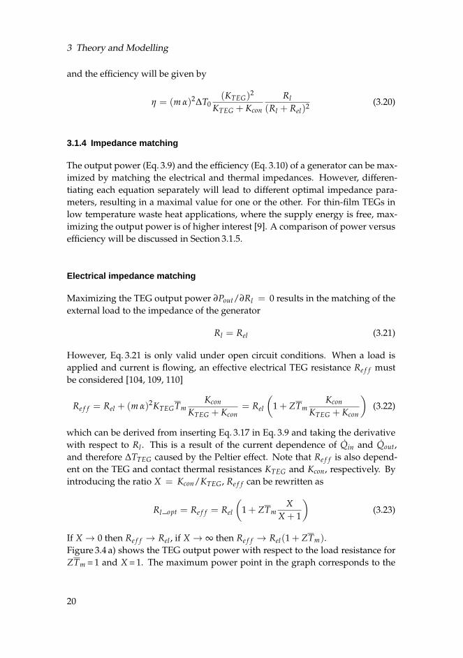
3.1.4 Impedance matching
The output power (Eq. 3.9) and the efficiency (Eq. 3.10) of a generator can be max-imized by matching the electrical and thermal impedances. However, differen-tiating each equation separately will lead to different optimal impedance para-meters, resulting in a maximal value for one or the other. For thin-film TEGs inlow temperature waste heat applications, where the supply energy is free, max-imizing the output power is of higher interest [9]. A comparison of power versusefficiency will be discussed in Section 3.1.5.
Electrical impedance matching
Maximizing the TEG output power ∂Pout/∂Rl = 0 results in the matching of theexternal load to the impedance of the generator
Rl = Rel (3.21)
However, Eq. 3.21 is only valid under open circuit conditions. When a load isapplied and current is flowing, an effective electrical TEG resistance Re f f mustbe considered [104, 109, 110]
Re f f = Rel + (m α)2KTEGTmKcon
KTEG + Kcon= Rel
(
1 + ZTmKcon
KTEG + Kcon
)
(3.22)
which can be derived from inserting Eq. 3.17 in Eq. 3.9 and taking the derivativewith respect to Rl . This is a result of the current dependence of Qin and Qout,and therefore ∆TTEG caused by the Peltier effect. Note that Re f f is also depend-ent on the TEG and contact thermal resistances KTEG and Kcon, respectively. Byintroducing the ratio X = Kcon/KTEG, Re f f can be rewritten as
Rl_opt = Re f f = Rel
(
1 + ZTmX
X + 1
)
(3.23)
If X → 0 then Re f f → Rel , if X → ∞ then Re f f → Rel(1 + ZTm).Figure 3.4 a) shows the TEG output power with respect to the load resistance forZTm = 1 and X = 1. The maximum power point in the graph corresponds to the
20

3.1 Thermoelectric generators
Rl[Ohm]
a)
=RelRl =ReffRl
KTEG_opt
K [cm K/W]TEG
2
b)
KTEG
=Kcon
TE
G o
utp
ut pow
er
[mW
/cm
]2
Max
TE
G o
utp
ut pow
er
[mW
/cm
]2
Figure 3.4: a) TEG output power as a function of the load resistance Rl for ZTm = 1and X = 1. b) TEG output power as a function of the generator’s thermal resist-ance KTEG. For the change of KTEG, the TC length lTEG was varied. The simu-lations were performed for a Kcon = 2.35 cm2K/W and ∆T0 = 10 K, the remainingparameters are found in Tab. B.1 in App. B. The optimal load and thermal TEGresistance differ from the impedance matching of the open circuit solution.
maximal TEG output power under matched effective electrical load
Pmax = (m α ∆T0)2(
KTEG
KTEG + Kcon
)2 14Re f f
=(m α ∆T0)
2
4Re f f
(
11 + X
)2
(3.24)
To show the impact of Re f f in comparison to the often used load matching foropen circuit conditions [111–114] from Eq. 3.21, the relative increase of the out-put power ∆Pmax for Rl = Re f f is calculated for different ZTm and X values andsummarized in Table 3.1. The parameter combination closest to the experimental
Table 3.1: Impact of Re f f on Pout for different ZTm and X (Rel = 0.62 Ω). Bold val-ues mark the parameter combination closest to the experimental measurementsin Chap. 5.
ZTm [-] X [-] Re f f [Ω] ∆Pout [%]
1 1 0.93 4.20.5 1 0.78 1.20.2 1 0.68 0.2
1 20 1.21 11.60.5 20 0.91 3.90.2 20 0.74 0.8
21
3 Theory and Modelling
measurements performed in this thesis is marked in bold. It can be concludedthat at this operating point, the introduced error is negligible. However, forhigher ZTm and X values, e.g. in energy harvesting applications for autonomoussystems, Re f f should be considered as a relevant parameter for system optimiza-tion.
Thermal impedance matching
Equivalent to the electrical load matching, also thermal resistance matching canbe applied. If a certain thermal contact resistance Kcon is given, the TEG thermalresistance KTEG can be adapted to further maximize the output power of a TEG.
In the simplified model under open circuit conditions, the maximal power canbe expressed by replacing Rl = Rel with m2 α2 KTEG / Zm according to Eq. 3.7
Pout =∆T2
0 Z
4KTEG
(KTEG + Kcon)2 (3.25)
Maximizing the TEG output power ∂Pout/∂KTEG = 0 yields [30, 115]
KTEG = Kcon (3.26)
If a current is running and the effective ∆TTEG is reduced by the Peltier effect, theoptimal KTEG can be calculated from [78, 89, 110]
KTEG_opt = Kcon
√
1 + ZTm (3.27)
and the optimal Re f f becomes in the case of a thermally matched system
Re f f _opt = Rel
√
1 + ZTm (3.28)
resulting in a maximal output power
Pmax_opt =∆T2
0 Zm
4 KTEG
1
(1 +√
1 + ZTm)2(3.29)
Figure 3.4 b) shows the output power with respect to the thermal TEG resistancefor a module with ZTm = 1. For small ZTm, the difference between the power atKTEG = Kcon and KTEG_opt will again become negligibly small.
Note that the thermal impedance matching works only by adapting KTEG to
22
3.1 Thermoelectric generators
Kcon and not vice-versa. Reducing Kcon independent of KTEG will always lead toa higher output power.
3.1.5 TEG model conclusions and considerations
The above presented model allows us to highlight important design aspects rel-evant for this work. In the following section, the impact of the thermal contactresistance, the geometric parameters of the module and the different thermoelec-tric material parameters on the TEG output performance will be discussed.
Impact of thermal contact resistance
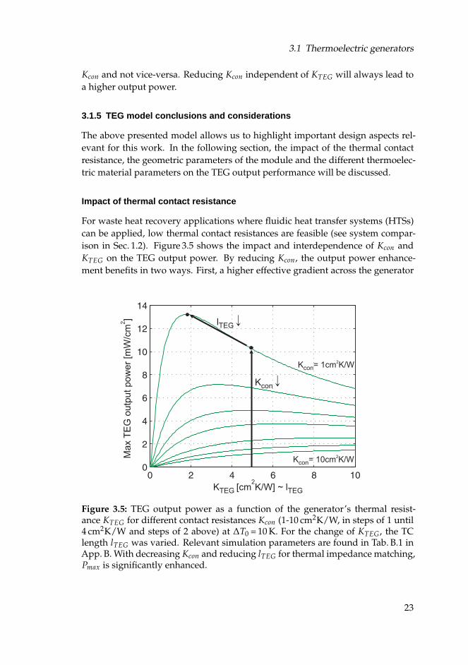
For waste heat recovery applications where fluidic heat transfer systems (HTSs)can be applied, low thermal contact resistances are feasible (see system compar-ison in Sec. 1.2). Figure 3.5 shows the impact and interdependence of Kcon andKTEG on the TEG output power. By reducing Kcon, the output power enhance-ment benefits in two ways. First, a higher effective gradient across the generator
K [cm K/W] ~ lTEG
2
TEG
lTEG↓
Kcon↓
K = 1cm K/Wcon2
K = 10cm K/Wcon2M
ax
TE
G o
utp
ut
po
we
r [m
W/c
m]
2
Figure 3.5: TEG output power as a function of the generator’s thermal resist-ance KTEG for different contact resistances Kcon (1-10 cm2K/W, in steps of 1 until4 cm2K/W and steps of 2 above) at ∆T0 = 10 K. For the change of KTEG, the TClength lTEG was varied. Relevant simulation parameters are found in Tab. B.1 inApp. B. With decreasing Kcon and reducing lTEG for thermal impedance matching,Pmax is significantly enhanced.
23
3 Theory and Modelling
thus a higher power output (see Eq. 3.18 and Eq. 3.29) can be reached, correspond-ing to the vertical arrow in the center of Figure 3.5. Second, it allows for a re-duction of KTEG by decreasing the TC length, i.e. generator thickness, to reach athermally matched system (diagonal arrow to upper left). By decreasing the thick-ness of the TEG to the micrometer range, the heat flux through the generator issignificantly increased. This enables the application of thin-film generators, sav-ing material, weight and cost.
Optimal TEG geometrical parameters
The thermal and electrical resistance of a generator depends not only on materialproperties, but also on geometrical parameters (see Eq. B.1 - Eq. B.6 in App. B).The two main geometrical parameters, the TC length lTEG and TC diameterdTEG, can be adjusted to maximize the power output by electrical and thermalimpedance matching. Additionally, the spacing between the piles s, i.e. the piledensity must be considered. This can be expressed with the ratio between theinactive (e.g. air or polymer mold) and active (TC) material of the generator AV.For a fixed area of the TEG, the corresponding number of thermocouples can becalculated from the diameter and the AV-ratio (see Eq. B.2 in App. B).
When the interconnect resistance Ric of the module is neglected, the outputpower per area for a fixed AV-ratio is independent of the diameter as shownin [27, 114] (see dashed green line in Fig. 3.6 a)). In this ideal case, only areduction of the AV-ratio will lead to a power increase. In a more realistic case,where interconnect resistances are considered, minimizing the diameter (i.e.maximizing the number of TCs) will enhance the output power as indicated bythe dotted green line in Figure 3.6 a). This can be explained with a smaller Ric perTC for smaller diameters, resulting from a shorter spacing between the piles fora constant AV-ratio. With increasing thickness of the interconnect, i.e. reductionof Ric, this effect will become less pronounced.In practice, however, it is difficult to maintain a constant AV when the diameter
is reduced. The limiting factor caused by fabrication constrains is the minimaldistance between the pile s. By fixing s to a certain minimal value, an optimaldiameter can be found, as shown by the green solid line in Figure 3.6 a). Fora specific contact resistance, geometric constrains of s and material propertiesof the module, an optimal combination of the TC length lTEG and diameterdTEG will result in an optimal output power as indicated in Figure 3.6 b). Withdecreasing TC length, the electrical resistance of the module Rel will decreaseand thus its negative impact on the output power will be reduced. Therefore,smaller TC diameters and thus a larger amount of TCs will be favorable.
24
3.1 Thermoelectric generators
d [mm]TEG
AV
[-]
dTEG_opt
P for fixed s
P for fixed AV
P for fixed AV no R
AV for fixed sAV fixed
out
out
out ic
a)
Max
TE
G o
utp
ut pow
er
[mW
/cm
]2
d [mm]TEG
dTEG_opt at l optTEG_
b)
lTEG= 150µm
lTEG= 550µm
Max
TE
G o
utp
ut pow
er
[mW
/cm
]2
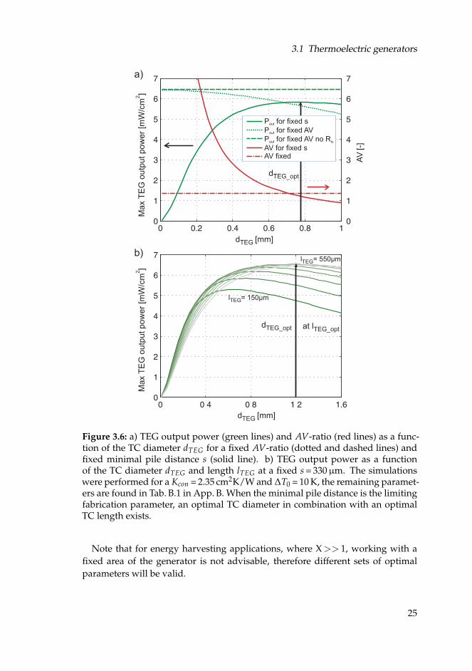
Figure 3.6: a) TEG output power (green lines) and AV-ratio (red lines) as a func-tion of the TC diameter dTEG for a fixed AV-ratio (dotted and dashed lines) andfixed minimal pile distance s (solid line). b) TEG output power as a functionof the TC diameter dTEG and length lTEG at a fixed s = 330µm. The simulationswere performed for a Kcon = 2.35 cm2K/W and ∆T0 = 10 K, the remaining paramet-ers are found in Tab. B.1 in App. B. When the minimal pile distance is the limitingfabrication parameter, an optimal TC diameter in combination with an optimalTC length exists.
Note that for energy harvesting applications, where X>> 1, working with afixed area of the generator is not advisable, therefore different sets of optimalparameters will be valid.
25
3 Theory and Modelling
Impact of thermal conductivity
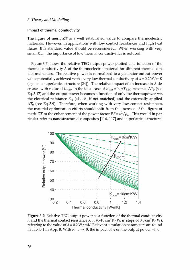
The figure of merit ZT is a well established value to compare thermoelectricmaterials. However, in applications with low contact resistances and high heatfluxes, this standard value should be reconsidered. When working with verysmall Kcon, the importance of low thermal conductivities is reduced.
Figure 3.7 shows the relative TEG output power plotted as a function of thethermal conductivity λ of the thermoelectric material for different thermal con-tact resistances. The relative power is normalized to a generator output powervalue potentially achieved with a very low thermal conductivity of λ = 0.2 W/mK(e.g. in a superlattice structure [24]). The relative impact of an increase in λ de-creases with reduced Kcon. In the ideal case of Kcon = 0, ∆TTEG becomes ∆T0 (seeEq. 3.17) and the output power becomes a function of only the thermopower mα,the electrical resistance Rel (also Rl if not matched) and the externally applied∆T0 (see Eq. 3.9). Therefore, when working with very low contact resistances,the material optimization efforts should shift from the increase of the figure ofmerit ZT to the enhancement of the power factor PF = α2/ρel . This would in par-ticular refer to nanostructured composites [116, 117] and superlattice structures
Thermal conductivity [W/mK]
K = 10cm K/Wcon2
K = 0cm K/Wcon2
Kcon↓
Figure 3.7: Relative TEG output power as a function of the thermal conductivityλ and the thermal contact resistance Kcon (0-10 cm2K/W, in steps of 0.5 cm2K/W),referring to the value of λ = 0.2 W/mK. Relevant simulation parameters are foundin Tab. B.1 in App. B. With Kcon → 0, the impact of λ on the output power → 0.
26
3.1 Thermoelectric generators
[24, 25, 118], where an improvement of ZT is mainly achieved by the reduction ofλ. This conclusion is in agreement with [119], where the much higher relevanceof the power factors over the ZT value, especially for high heat flux applications,was also emphasized.
Maximal power vs. efficiency
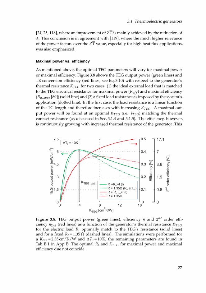
As mentioned above, the optimal TEG parameters will vary for maximal poweror maximal efficiency. Figure 3.8 shows the TEG output power (green lines) andTE conversion efficiency (red lines, see Eq. 3.10) with respect to the generator’sthermal resistance KTEG for two cases: (1) the ideal external load that is matchedto the TEG electrical resistance for maximal power (Re f f ) and maximal efficiency(Rη_max [89]) (solid line) and (2) a fixed load resistance as imposed by the system’sapplication (dotted line). In the first case, the load resistance is a linear functionof the TC length and therefore increases with increasing KTEG. A maximal out-put power will be found at an optimal KTEG (i.e. lTEG) matching the thermalcontact resistance (as discussed in Sec. 3.1.4 and 3.1.5). The efficiency, however,is continuously growing with increased thermal resistance of the generator. This
K [cm K/W]TEG
2
Effic
iency
[%]
KTEG_opt R =R
R = 1.35 (R at l )
R = R =f (l)
R = 1.35
l eff
l eff opt
l
l
=f (l)
Ω
Ω
η_max
17.1
7
3.6
1.9
0.8
0
2ord
er
effic
iency
[%]
nd
TE
G o
utp
ut
po
we
r [m
W/c
m]
2
ΔT = 10K0
Figure 3.8: TEG output power (green lines), efficiency η and 2nd order effi-ciency η2nd (red lines) as a function of the generator’s thermal resistance KTEG
for the electric load Rl optimally match to the TEG’s resistance (solid lines)and for a fixed Rl = 1.35 Ω (dashed lines). The simulations were performed fora Kcon = 2.35 cm2K/W and ∆T0 = 10 K, the remaining parameters are found inTab. B.1 in App. B. The optimal Rl and KTEG for maximal power and maximalefficiency due not coincide.
27
3 Theory and Modelling
can be explained most directly with the basic open circuit model. By enteringRl = Rg (Eq. 3.21) in Eq. 3.20 and replacing Rl with m2 α2 KTEG / Zm (Eq. 3.7), theefficiency can be simplified to
η =Zm ∆T0
4KTEG
KTEG + Kcon(3.30)
Therefore, with increasing KTEG, η will asymptotically converge to the maximaltheoretical value of Zm∆T0/4. For a given load resistance, an optimal KTEG orTEG thickness will exist, where the efficiency is maximal. This, however, doesnot correspond to the optimal thickness for maximal power.
To put the thermal efficiency in perspective with the theoretically reachablevalue limited by the Carnot efficiency, the scale of the 2nd order efficiency η2nd
(see Eq. 3.11) is added in Figure 3.8. Since the Carnot efficiency is dependent on∆TTEG, the scales of η and η2nd are not linear.
3.2 Micro heat transfer system
The second component of the thermoelectric heat exchanger is the micro heattransfer system (µHTS), which is responsible for the thermal coupling of the TEGto the hot and cold fluid. The following section will review the basic fluid dy-namic theory as well as describe the modelling of the system.
3.2.1 Fluid dynamics in confined ducts
As a basis for the micro heat transfer system model, the fundamental theorybehind convective heat transfer and hydrodynamic losses in confined ducts willbe introduced.
In order to characterize the relevant flow regimes, i.e. distinguish betweenlaminar and turbulent flow, the dimensionless Reynolds number (Re) is used.The Reynolds number describes the balance between viscous and inertial forces,and therefore relates to flow instability
Re =u dch
ν(3.31)
where u is the mean velocity of the fluid, dch is the characteristic length ofthe channel and ν is the kinematic viscosity of the fluid. In circular ducts, thetransition from laminar to turbulent flow starts at Re ≈ 2300, but fully turbulentconditions are reached at much higher Reynolds numbers (Re ≈ 10000) [120].
28
3.2 Micro heat transfer system
For rectangular ducts, the transition depends on the channel aspect ratio andcan vary between 1850 and 2800 [121]. In microsystems, where the characteristiclength scales are typically very small (dch ∼ 10−6), the Reynolds number usuallylies well below this transition point.
Another important consideration is to distinguish between a developing flowin the duct entrance region, and a fully developed flow. This distinction is relev-ant for the selection of an appropriate heat transfer model, as well as a frictionmodel for pressure drop calculations. In short channels as in the discussed µHTS,the total channel length can be smaller than the hydrodynamic and thermal en-trance region.
Hydrodynamics
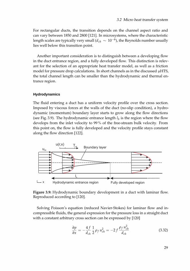
The fluid entering a duct has a uniform velocity profile over the cross section.Imposed by viscous forces at the walls of the duct (no-slip condition), a hydro-dynamic (momentum) boundary layer starts to grow along the flow directions(see Fig. 3.9). The hydrodynamic entrance length lh is the region where the flowdevelops from the inlet velocity to 99 % of the free-stream bulk velocity. Fromthis point on, the flow is fully developed and the velocity profile stays constantalong the flow direction [122].
Hydrodynamic entrance region Fully developed region
uIN
TWu(r,x)
Boundary layer
lh
x
Figure 3.9: Hydrodynamic boundary development in a duct with laminar flow.Reproduced according to [120].
Solving Poisson’s equation (reduced Navier-Stokes) for laminar flow and in-compressible fluids, the general expression for the pressure loss in a straight ductwith a constant arbitrary cross section can be expressed by [120]
∂p
∂x= − 4 f
dch
12
ρ f u2ch = −2 f
ρ f u2ch
dch(3.32)
29
3 Theory and Modelling
where uch is the mean fluid velocity, ρ f is the density of the fluid and f isthe Fanning friction factor. In non-circular ducts, the characteristic length dch
corresponds to the hydraulic diameter. It has been shown, however, that in alaminar flow regime it is more precise to use the square root of the cross sectionalarea rather than the hydraulic diameter [123].
In order to distinguish the friction factor in developing flow ( f ) from the onein the fully developed flow, an apparent friction factor fapp was introduced [122].Additionally to shear stress at the wall, the pressure drop in a developing flowis also caused by fluid acceleration. An expression of the apparent friction factorfor laminar developing flow in non-circular ducts is provided by [124, 125] (seeEq. B.11 in App. B).
Convective heat transfer
Convection is a heat transfer mechanism by a fluid in motion. It describes thecombined effects of heat conduction due to molecular interactions (i.e. diffusion)and energy transport by the bulk fluid flow motion [120].
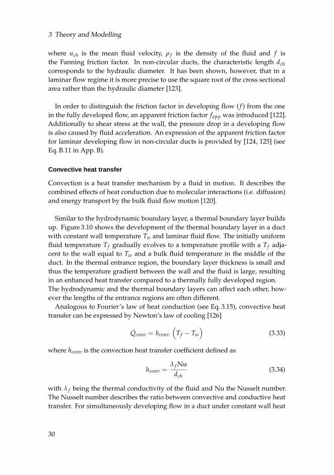
Similar to the hydrodynamic boundary layer, a thermal boundary layer buildsup. Figure 3.10 shows the development of the thermal boundary layer in a ductwith constant wall temperature Tw and laminar fluid flow. The initially uniformfluid temperature Tf gradually evolves to a temperature profile with a Tf adja-cent to the wall equal to Tw and a bulk fluid temperature in the middle of theduct. In the thermal entrance region, the boundary layer thickness is small andthus the temperature gradient between the wall and the fluid is large, resultingin an enhanced heat transfer compared to a thermally fully developed region.The hydrodynamic and the thermal boundary layers can affect each other, how-ever the lengths of the entrance regions are often different.
Analogous to Fourier’s law of heat conduction (see Eq. 3.15), convective heattransfer can be expressed by Newton’s law of cooling [126]
Qconv = hconv
(
Tf − Tw
)
(3.33)
where hconv is the convection heat transfer coefficient defined as
hconv =λ f Nu
dch(3.34)
with λ f being the thermal conductivity of the fluid and Nu the Nusselt number.The Nusselt number describes the ratio between convective and conductive heattransfer. For simultaneously developing flow in a duct under constant wall heat
30
3.2 Micro heat transfer system
Thermal entrance region Fully developed region
TW > TINTIN
TWTIN
Boundary layer
x
Figure 3.10: Thermal boundary development in a heated duct with constant walltemperature and laminar flow. Reproduced according to [120].
flux boundary condition, a Nusselt number correlation was provided by [127](see Eq. B.12 in App. B for exact Nu definition).
Microfluidic considerations
From Eq. 3.32 and Eq. 3.34 it can be deducted that reducing the channel dimen-sions to the micrometre scale will significantly increase the heat transfer coef-ficient as well as the pressure losses. Additionally, an increase of the effectiveheat exchange area by high aspect ratio microchannels will further enhance thethermal performance. By decreasing the microchannel dimensions, the questionarises until which point the classic theory based on thermodynamic equilibriumand continuum, formulated from the observation of macroscopic flow and heattransfer processes, is still valid. The onset of its failure has been widely discussed;however it is not well defined for liquids in microchannels. Many authors reportlarge deviation from the conventional theory [128–130] attributing it to several mi-croscale phenomena such as surface roughness [131–133], viscous heating effects[134], electrokinetic forces [135] or an early transition from laminar to turbulentflow [131, 136]. On the other hand, various papers confirm the validity of theclassic theory [32, 137–144] for channel length scales as low as 4.5µm [145].Concluding from the inconsistent published results, potential microscale effectsmust be kept in mind.
3.2.2 Basic micro heat transfer system model
The generic part of the one-dimensional µHTS model is based on [44, 146].Therefore, only the basic concept will be described in this section, further detailscan be found in [44, 146]. The introduced model extensions and optimizationswill be covered in more detail in the following section.
31
3 Theory and Modelling
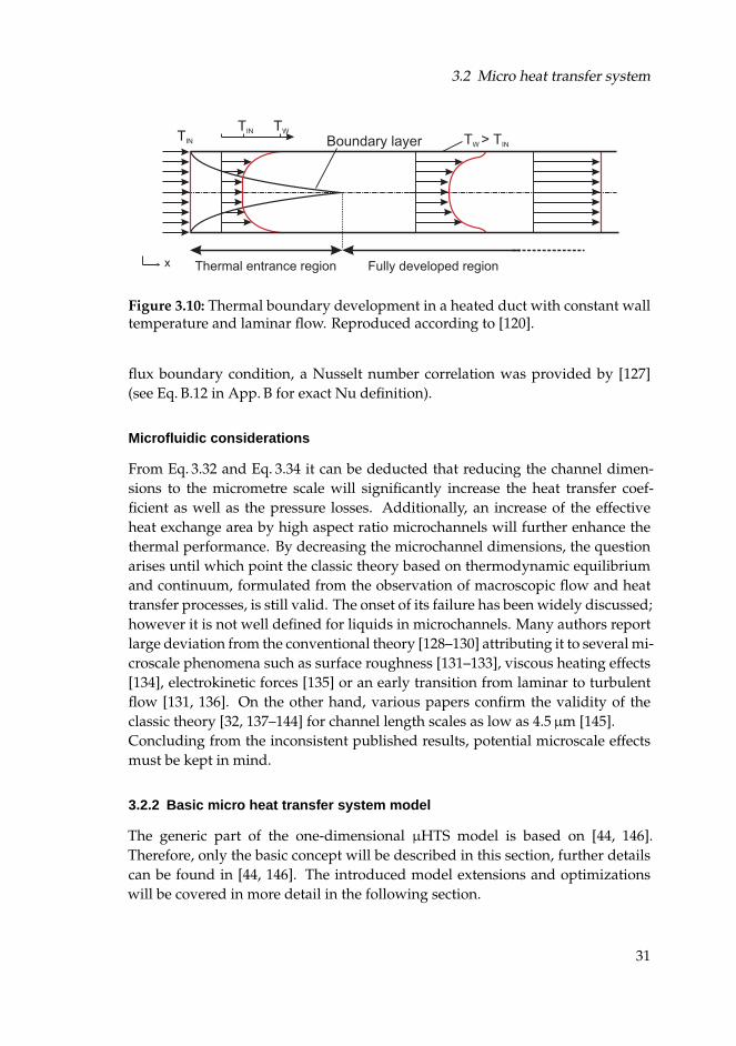
Analogous to the theory section above, the model is divided in two parts: athermal and a hydrodynamic model. Figure 3.11 depicts the schematic cross sec-tion of the µHTS and of a periodic microchannel unit cell showing the thermaland hydrodynamic model contributions and relevant design parameters.
Cu micro-channels
Manifoldchannels
Periodic unit cell
Manifoldbase
Δpnoz
Δpmani
Δpe
Δpch
Δpc
Manifoldoutlet
Manifold inlet
luc
hmc
Slot
lnoz
tbase
wnoz/2
Kcnd
Kcnv
Khc
Tin
Tw
wch
Periodic unit cellside view
wfin/2
Figure 3.11: Schematics of the µHTS with an enlargement of the microchannelunit cell showing the thermal and hydrodynamic model contributions and relev-ant design parameters.
32
3.2 Micro heat transfer system
Thermal model
The thermal model of the µHTS is based on the concept of a thermal resistancenetwork simplified to one-dimensional heat transfer. It is assumed that the heattransfer takes place only inside the copper microchannels and that no heat ex-change occurs between the channels and the polymer manifold (i.e. adiabaticboundary conditions).The total heat transfer resistance KHTS of the µHTS consists of the conductiveresistance through the microchannels Kcnd, the convective resistance at the fluid-channel interface Kcnv, and the fluid resistance due to its limited heat capacity Khc
(compare unit cell in Fig. 3.11)
KHTS = Kcnd + Kcnv + Khc (3.35)
The conductive resistance term is given by
Kcnd =tbase
λCu(3.36)
where tbase is the thickness of the microchannel chip base and λCu is the thermalconductivity of copper. Due to the a large value of λCu, the contribution of Kcnd
to KHTS is small.
The convective thermal resistance is composed of three main parts: convectionat (1) the base, (2) at the fins and (3) at the fin top in the channel entrance region.The last term was added to the original version in [44, 146], based on findingsfrom 3D-FEM simulation results of the microchannel unit cell (see Sec. 3.2.4 formore details).
Kcnv =Auc
hbase Abase + 2 η f h f in A f in + h f in_top A f in_top
(3.37)
where hbase, h f in and h f in_top are the average convective heat transfer coeffi-cients of the base, fin and the fin top, respectively, Axy are the correspondingsurface areas and η f is the fin efficiency (see Eq. B.14 in App. B for the exactdefinition). The Nusselt number correlation for laminar developing flow are im-plemented according to [127] and for laminar jet impingement according to [147].
The bulk fluid resistance Khc caused by the heating up of the fluid as it absorbsenergy flowing through the channel, is expressed as
Khc =Auc
cp ρ f Vmc(3.38)
33
3 Theory and Modelling
where cp is the mean specific heat capacity of the fluid, ρ f is the fluid density and
Vmc is the volumetric flow rate through the microchannel.
Hydrodynamic model
The pressure losses in the µHTS are composed of the losses inside the microchan-nel unit cell ∆pmc and the tapered manifold distribution channels ∆pman. In theunit cell, several pressure drops contribute to the overall ∆pmc: the frictional pres-sure losses in the straight microchannel ∆pch as well as in the inlet and outletnozzles ∆pnoz, and the pressure losses induced by sudden expansion and con-striction at the microchannel entrance ∆pe and exit ∆pc (see microchannel unitcell in Fig. 3.11).
∆pmc = ∆pch + 2 ∆pnoz + ∆pc + ∆pe (3.39)
The expressions for the different pressure drop contributions in straight parts ofthe microchannel are based on Eq. 3.32 from Section 3.2.1 and are defined as [148]
∆pch =2 fapp_ch ρ f u2
ch lch
dch(3.40)
∆pnoz =2 fapp_noz ρ f u2
noz lnoz
dnoz(3.41)
(3.42)
The losses related to sudden expansion and constriction can be formulated as[149]
∆pc =12
ρ f
(
u2narrow − u2
noz
)
+12
Cc ρ f u2narrow (3.43)
∆pe =12
ρ f
(
u2narrow − u2
noz
)
+12
Ce ρ f u2noz (3.44)
where unarrow is the mean velocity right at the channel entrance after leavingthe nozzle and Cc and Ce are the loss coefficients associated with the abruptcontraction and expansion according to [149, 150].
The pressure drop in the tapered manifold is a function of the channel posi-tion, due to the varying channel width and continuous fluid outflow along themanifold channel
∆pman = −2∫ Lman
0
fapp_mani(x) ρ f u2man(x)
dman(x)dx (3.45)
To solve the integral numerically, the manifold channel is divided into Nch
subdivisions with the length of wch + w f in.
34
3.2 Micro heat transfer system
The pumping power of the µHTS was computed by multiplying the total hy-drodynamic resistance ∆pHTS by the volumetric fluid flow V
Pp = ∆pHTS V = (∆pmc + ∆pman) V (3.46)
3.2.3 Model extensions
In order to model the µHTS more precisely, temperature changes inside mi-crochannel and the manifold channel were added to the existing model.
Temperature profile inside the microchannels
Changes of the fluid temperature inside the microchannel have an impact onthe fluid properties (in particular the fluid viscosity) and therefore the hydro-dynamic and thermal performance of the system. Additionally, by introducing atemperature profile, the microchannel outlet temperature can be computed andused for the estimation of the inlet fluid temperature change along the manifoldchannel (see next section).
For this purpose, the microchannel unit cell was divided into an entrance re-gion underneath the inlet nozzle (dark gray area in inset of Fig. 3.12 a)), a hori-zontal flow region along the microchannel (light gray area in insert of Fig. 3.12 a))and an exit region (white area in inset of Fig. 3.12 a)). The regions are discret-ized into horizontal and vertical elements, respectively. The temperature of eachelement is calculated according to
Ti+1 = Ti + qi1
micp,i= Ti +
Ai dx hi (Tw − Ti)
Vch ρi cp,i(3.47)
where Ti is the local fluid temperature, qi is the local heat flux from the channelbase and fins, Ai is the local heat transfer area, dx is the length of the subdivisionand hi is the local convective heat transfer coefficient. A constant temperature atthe copper channel walls Tw is assumed, corresponding to the temperature at thechannel base. For the calculations of Kcnv, the average convective heat transfercoefficient of all elements is used.
Figure 3.12 a) shows the temperature profile along the flow path inside amicrochannel unit cell computed by 3D-FEM simulations and by the one-dimensional model. The first region corresponds to the nozzle inlet, wherethe heat flux from the manifold base is negligible. The heat transfer in theentrance region is affected by jet impingement at the fin top and channel base,
35
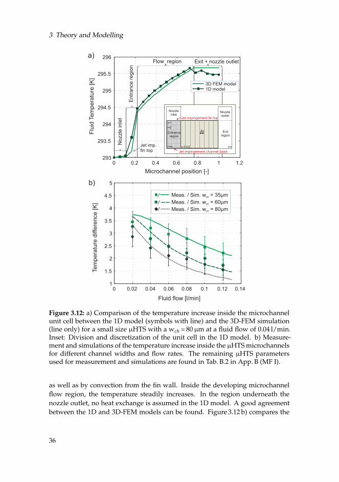
3 Theory and Modelling
0 0.2 0.4 0.6 0.8 1 1.2293
293.5
294
294.5
295
295.5
296
Microchannel position [-]
Flu
idTem
pera
ture
[K
]
a)
No
zzle
in
let
En
tra
nce
re
gio
n
Flow region Exit + nozzle outlet
dx
i=1 i=n
i=1
i=2
i=m
Nozzleinlet
Nozzleoutlet
i=2
Jet impingement fin top
Jet impingement channel base
Exitregion
Entranceregion
3D FEM model1D model
Jet imp.fin top
0 0.02 0.04 0.06 0.08 0.1 0.12 0.141
1.5
2
2.5
3
3.5
4
4.5
5
Fluid flow [l/min]
Tem
pera
ture
diffe
rence [K
]
Meas. / Sim. w = 35µmch
Meas. / Sim. w = 60µm
Meas. / Sim. w = 80µmch
ch
b)
Figure 3.12: a) Comparison of the temperature increase inside the microchannelunit cell between the 1D model (symbols with line) and the 3D-FEM simulation(line only) for a small size µHTS with a wch = 80µm at a fluid flow of 0.04 l/min.Inset: Division and discretization of the unit cell in the 1D model. b) Measure-ment and simulations of the temperature increase inside the µHTS microchannelsfor different channel widths and flow rates. The remaining µHTS parametersused for measurement and simulations are found in Tab. B.2 in App. B (MF I).
as well as by convection from the fin wall. Inside the developing microchannelflow region, the temperature steadily increases. In the region underneath thenozzle outlet, no heat exchange is assumed in the 1D model. A good agreementbetween the 1D and 3D-FEM models can be found. Figure 3.12 b) compares the
36
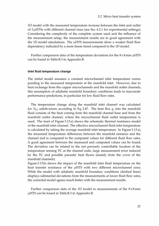
3.2 Micro heat transfer system
1D model with the measured temperature increase between the inlet and outletof 3µHTSs with different channel sizes (see Sec. 4.2.1 for experimental settings).Considering the complexity of the complete system used and the influence ofthe measurement setup, the measurement results are in good agreement withthe 1D model simulations. The µHTS measurements show a weaker fluid flowdependency indicated by a more linear trend compared to the 1D model.
Further comparison data of the temperature deviations for the 8 x 8 mm µHTScan be found in Table B.3 in Appendix B.
Inlet fluid temperature change
The initial model assumes a constant microchannel inlet temperature corres-ponding to the measured temperature at the manifold inlet. However, due toheat exchange from the copper microchannels and the manifold outlet channels,this assumption of adiabatic manifold boundary conditions leads to inaccurateperformance predictions, in particular for low fluid flow rates.
The temperature change along the manifold inlet channel was calculatedfor Nch subdivisions according to Eq. 3.47. The heat flux qi into the manifoldfluid consists of the heat coming from the manifold channel base and from themanifold outlet channel, where the microchannel fluid outlet temperature isused. The inset of Figure 3.13 a) shows the schematic thermal resistance modelof the manifold inlet channel. The effective microchannel fluid inlet temperatureis calculated by taking the average manifold inlet temperature. In Figure 3.13 a),the measured temperature differences between the manifold entrance and thechannel end is compared to the computed values for different fluid flow rates.A good agreement between the measured and computed values can be found.The deviation can be related to the not precisely controllable location of thetemperature sensing TC at the channel ends, large measurement error inducedby the TC and possible parasitic heat fluxes (mainly from the cover of themanifold channels).Figure 3.13 b) shows the impact of the manifold inlet fluid temperature on theheat transfer resistance of the µHTS with two different microchannel sizes.While the model with adiabatic manifold boundary conditions (dashed lines)displays substantial deviations from the measurements at lower fluid flow rates,the corrected model agrees much better with the measurement results.
Further comparison data of the 1D model to measurements of the 8 x 8 mmµHTS can be found in Table B.3 in Appendix B.
37
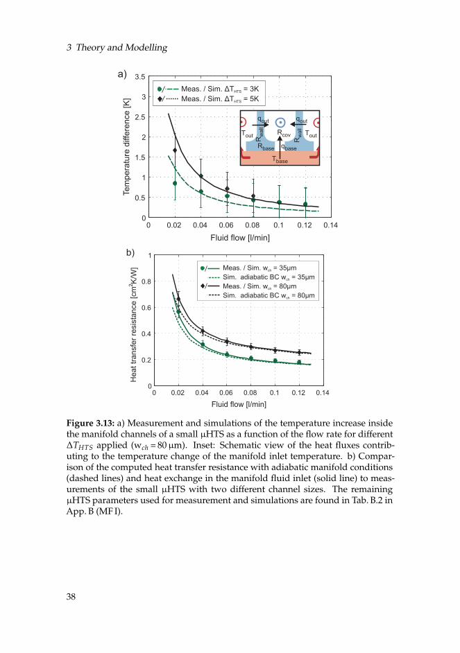
3 Theory and Modelling
0 0.02 0.04 0.06 0.08 0.1 0.12 0.140
0.5
1
1.5
2
2.5
3
3.5
Fluid flow [l/min]
Tem
pera
ture
diffe
rence [K
]
Meas. / Sim. T = 3K
Meas. / Sim. T = 5KHTS
HTS
Δ
Δ
a)
Tout
qbase
Tout
qoutqout
Rcov
Rbase
Rw
all
Rw
all
Tbase
0 0.02 0.04 0.06 0.08 0.1 0.12 0.140
0.2
0.4
0.6
0.8
1
Fluid flow [l/min]
Heat tr
ansfe
r re
sis
tance [cm
2K
/W]
b)
Meas. / Sim. w = 35µm
diabatic BCch
Sim. a w = 35µm
Meas. / Sim. w = 80µm
Sim. adiabatic BC w = 80µm
ch
ch
ch
Figure 3.13: a) Measurement and simulations of the temperature increase insidethe manifold channels of a small µHTS as a function of the flow rate for different∆THTS applied (wch = 80µm). Inset: Schematic view of the heat fluxes contrib-uting to the temperature change of the manifold inlet temperature. b) Compar-ison of the computed heat transfer resistance with adiabatic manifold conditions(dashed lines) and heat exchange in the manifold fluid inlet (solid line) to meas-urements of the small µHTS with two different channel sizes. The remainingµHTS parameters used for measurement and simulations are found in Tab. B.2 inApp. B (MF I).
38
3.2 Micro heat transfer system
3.2.4 3D FEM unit cell model
In order to compare and optimize the heat transfer and hydrodynamic propertiesof the 1D model as well as to evaluate the potential of different µHTS designimprovements, a 3D finite element method (FEM) model of the microchannelunit cell (see Fig. 3.11) was implemented in COMSOL Multiphysics r.
The coupled physics interfaces of the 3D model consist of (1) steady-stateincompressible Navier-Stokes with temperature dependent fluid variables and(2) general heat transfer for thermal conduction and convection. The majorpart of the simulations are performed with a symmetric half unit cell in orderto reduce computational time. For channels with asymmetric structures, theentire unit cell was simulated. The fluid boundary conditions are set to a fixedfluid velocity at the nozzle inlet, an open boundary at the outlet (equal to zeropressure) and no slip at the channel walls. For the thermal boundaries, a constantfluid inlet and channel base temperature (Tw) is set and isolation/symmetry areused for all remaining boundaries. The heat transfer resistance is calculated bydividing the applied temperature between the inlet and the base by the totaldissipated heat flux. The pressure losses are extracted from the average pressureat the nozzle inlet.
The parameter comparison between the 3D-FEM and the 1D model of the un-structured microchannels are found in Table B.3 in Appendix B.
µHTS design optimization
1By introducing microstructures and optimizing the fluid flow path inside themicrochannel unit cell, a reduction of the thermal and hydrodynamic resistancescan be achieved, leading to an overall increase in the power output of thethermoelectric heat exchanger (TEHEX).
Heat transfer enhancements can be achieved by increasing the convectivesurface area, augmenting the flow vorticity and limiting the growth of fluidicand thermal boundary layers [152]. For this purpose, two different microstruc-tures are integrated into the microchannels: an additional pin-fin structure andtriangular protrusions on the sidewall. While the first approach is expected toyield lower heat transfer resistances due to a higher convective surface area, thesecond one benefits from a simpler and more robust fabrication.Pressure losses can be reduced by a smart fluid path design. Avoiding abrupt
1 The content of the µHTS design optimization by 3D-FEM simulations was published in the pro-ceedings of Transducers 2013 [151] and was reproduced with permission. Copyright c© 2013 IEEE.
39
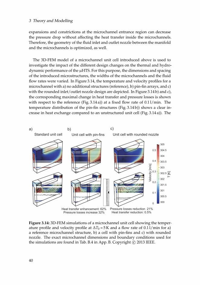
3 Theory and Modelling
expansions and constrictions at the microchannel entrance region can decreasethe pressure drop without affecting the heat transfer inside the microchannels.Therefore, the geometry of the fluid inlet and outlet nozzle between the manifoldand the microchannels is optimized, as well.
The 3D-FEM model of a microchannel unit cell introduced above is used toinvestigate the impact of the different design changes on the thermal and hydro-dynamic performance of the µHTS. For this purpose, the dimensions and spacingof the introduced microstructures, the widths of the microchannels and the fluidflow rates were varied. In Figure 3.14, the temperature and velocity profiles for amicrochannel with a) no additional structures (reference), b) pin-fin arrays, and c)with the rounded inlet/outlet nozzle design are depicted. In Figure 3.14 b) and c),the corresponding maximal change in heat transfer and pressure losses is shownwith respect to the reference (Fig. 3.14 a)) at a fixed flow rate of 0.1 l/min. Thetemperature distribution of the pin-fin structures (Fig. 3.14 b)) shows a clear in-crease in heat exchange compared to an unstructured unit cell (Fig. 3.14 a)). The
Heat transfer enhancement: 62%Pressure losses increase 32%
Pressure losses reduction 21%Heat transfer reduction: 0.5%
Unit cell with rounded nozzleStandard unit cell Unit cell with pin-fins
T[K
]
Velo
city [m
/s]
c)b)a)
305
304.5
304
303.5
303
302.5
302
301.5
301
300.5
300
0.5
0.4
0.3
0.2
0.1
0
Figure 3.14: 3D-FEM simulations of a microchannel unit cell showing the temper-ature profile and velocity profile at ∆T0 = 5 K and a flow rate of 0.1 l/min for a)a reference microchannel structure, b) a cell with pin-fins and c) with roundednozzle. The exact microchannel dimensions and boundary conditions used forthe simulations are found in Tab. B.4 in App. B. Copyright c© 2013 IEEE.
40
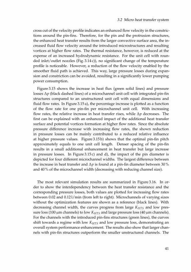
3.2 Micro heat transfer system
cross cut of the velocity profile indicates an enhanced flow velocity in the constric-tions around the pin-fins. Therefore, for the pin and the protrusion structures,the enhanced heat transfer results from the larger convective surface area, the in-creased fluid flow velocity around the introduced microstructures and resultingvortices at higher flow rates. The thermal resistance, however, is reduced at theexpense of an increased hydrodynamic resistance. For the unit cell with roun-ded inlet/outlet nozzles (Fig. 3.14 c)), no significant change of the temperatureprofile is noticeable. However, a reduction of the flow velocity enabled by thesmoother fluid path is achieved. This way, large pressure losses during expan-sion and constriction can be avoided, resulting in a significantly lower pumpingpower consumption.
Figure 3.15 shows the increase in heat flux (green solid lines) and pressurelosses ∆p (black dashed lines) of a microchannel unit cell with integrated pin-finstructures compared to an unstructured unit cell with equal dimensions andfluid flow rates. In Figure 3.15 a), the percentage increase is plotted as a functionof the flow rate for one pin-fin per microchannel unit cell. With increasingflow rates, the relative increase in heat transfer rises, while ∆p decreases. Thefirst can be explained with an enhanced impact of the additional heat transfersurface and potential vortices formation at higher flow rates. Since the absolutepressure difference increase with increasing flow rates, the shown reductionin pressure losses can be mainly contributed to a reduced relative influenceat higher pressure values. Figure 3.15 b) shows that the optimal pin-fin pitchapproximately equals to one unit cell length. Denser spacing of the pin-finresults in a small additional enhancement in heat transfer but large increasein pressure losses. In Figure 3.15 c) and d), the impact of the pin diameter isdepicted for four different microchannel widths. The largest difference betweenthe increase in heat transfer and ∆p is found at a pin-fin diameter between 30 %and 40 % of the microchannel width (decreasing with reducing channel size).
The most relevant simulation results are summarized in Figure 3.16. In or-der to show the interdependency between the heat transfer resistance and thecorresponding pressure losses, both values are plotted for increasing flow ratesbetween 0.02 and 0.12 l/min (from left to right). Microchannels of varying sizeswithout the optimization features are shown as a reference (black lines). Withdecreasing channel width, the curves progress from large KHTS and low pres-sure loss (100µm channels) to low KHTS and large pressure loss (40µm channels).For the channels with the introduced pin-fins structures (green lines), the curvesshift towards a regime with low KHTS and low pressure loss, demonstrating anoverall system performance enhancement. The results also show that larger chan-nels with pin-fin structures outperform the smaller unstructured channels. The
41
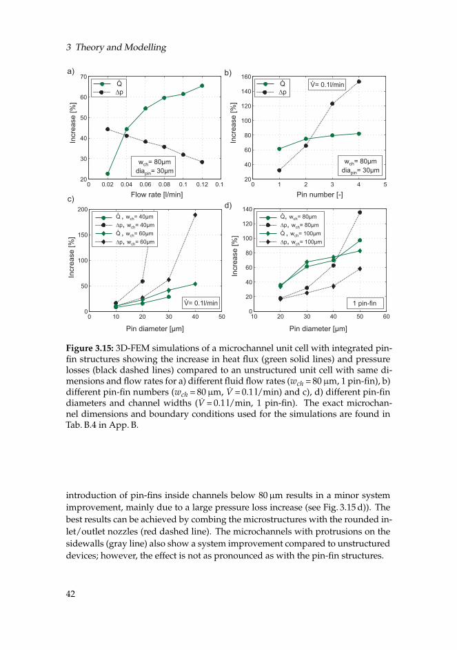
3 Theory and Modelling
0 0.02 0.04 0.06 0.08 0.1 0.12 0.1420
30
40
50
60
70In
cre
ase
[%
]
Pin diameter [µm]
Incre
ase
[%
]
Incre
ase
[%
]
0 1 2 3 4 520
40
60
80
100
120
140
160
Incre
ase
[%
]
b)a)
c)d)
w = 80µm
diach
pin= 30µm
w = 80µm
diach
pin= 30µm
V= 0.1l/minQ
Dp
Q
Dp
Flow rate [l/min] Pin number [-]
Pin diameter [µm]
0 10 20 30 40 500
50
100
150
200
V= 0.1l/min
10 20 30 40 500
20
40
60
80
100
120
140
60
1 pin-fin
Q , w = 40µm
p w = 40µm
Q w = 60µm
p w = 60µm
ch
ch
ch
ch
D
D
,,,
Q, w = 80µm
p w = 80µm
Q w = 100µm
p w = 100µm
ch
ch
ch
ch
D
D
,,,
Figure 3.15: 3D-FEM simulations of a microchannel unit cell with integrated pin-fin structures showing the increase in heat flux (green solid lines) and pressurelosses (black dashed lines) compared to an unstructured unit cell with same di-mensions and flow rates for a) different fluid flow rates (wch = 80µm, 1 pin-fin), b)different pin-fin numbers (wch = 80µm, V = 0.1 l/min) and c), d) different pin-findiameters and channel widths (V = 0.1 l/min, 1 pin-fin). The exact microchan-nel dimensions and boundary conditions used for the simulations are found inTab. B.4 in App. B.
introduction of pin-fins inside channels below 80µm results in a minor systemimprovement, mainly due to a large pressure loss increase (see Fig. 3.15 d)). Thebest results can be achieved by combing the microstructures with the rounded in-let/outlet nozzles (red dashed line). The microchannels with protrusions on thesidewalls (gray line) also show a system improvement compared to unstructureddevices; however, the effect is not as pronounced as with the pin-fin structures.
42
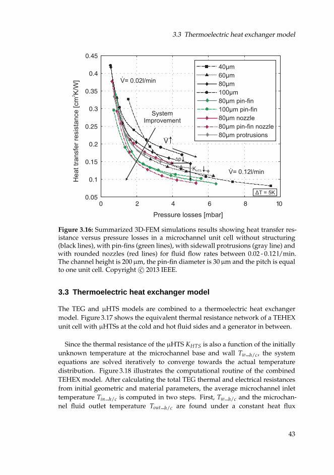
3.3 Thermoelectric heat exchanger model
V= 0.02l/min
V= 0.12l/min
V
SystemImprovement
40 mμ
μ
μ
μ
μ
μ
μ
μ
μ
60 m
80 m
100 m
80 m pin-fin
100 m pin-fin
80 m nozzle
80 m pin-fin nozzle
80 m protrusions
Δp
KHTS
ΔT = 5K
Pressure losses [mbar]
Heat tr
ansfe
r re
sis
tance [cm
K/W
]2
Figure 3.16: Summarized 3D-FEM simulations results showing heat transfer res-istance versus pressure losses in a microchannel unit cell without structuring(black lines), with pin-fins (green lines), with sidewall protrusions (gray line) andwith rounded nozzles (red lines) for fluid flow rates between 0.02 - 0.12 l/min.The channel height is 200µm, the pin-fin diameter is 30µm and the pitch is equalto one unit cell. Copyright c© 2013 IEEE.
3.3 Thermoelectric heat exchanger model
The TEG and µHTS models are combined to a thermoelectric heat exchangermodel. Figure 3.17 shows the equivalent thermal resistance network of a TEHEXunit cell with µHTSs at the cold and hot fluid sides and a generator in between.
Since the thermal resistance of the µHTS KHTS is also a function of the initiallyunknown temperature at the microchannel base and wall Tw_h/c, the systemequations are solved iteratively to converge towards the actual temperaturedistribution. Figure 3.18 illustrates the computational routine of the combinedTEHEX model. After calculating the total TEG thermal and electrical resistancesfrom initial geometric and material parameters, the average microchannel inlettemperature Tin_h/c is computed in two steps. First, Tw_h/c and the microchan-nel fluid outlet temperature Tout_h/c are found under a constant heat flux
43
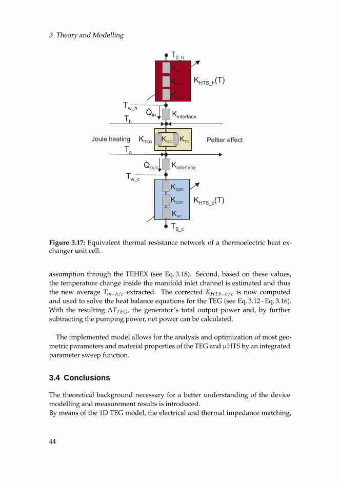
3 Theory and Modelling
KTEG
T0_h
Kinterface
KCOD
KCOV
KHC
KCOD
KCOV
KHC
KTCKISO
QIN
QOUT
Joule heating Peltier effect
KHTS_h(T)
Tw_h
Th
Tc
Kinterface
KHTS_c(T)
T0_c
Tw_c
Figure 3.17: Equivalent thermal resistance network of a thermoelectric heat ex-changer unit cell.
assumption through the TEHEX (see Eq. 3.18). Second, based on these values,the temperature change inside the manifold inlet channel is estimated and thusthe new average Tin_h/c extracted. The corrected KHTS_h/c is now computedand used to solve the heat balance equations for the TEG (see Eq. 3.12 - Eq. 3.16).With the resulting ∆TTEG, the generator’s total output power and, by furthersubtracting the pumping power, net power can be calculated.
The implemented model allows for the analysis and optimization of most geo-metric parameters and material properties of the TEG and µHTS by an integratedparameter sweep function.
3.4 Conclusions
The theoretical background necessary for a better understanding of the devicemodelling and measurement results is introduced.By means of the 1D TEG model, the electrical and thermal impedance matching,
44
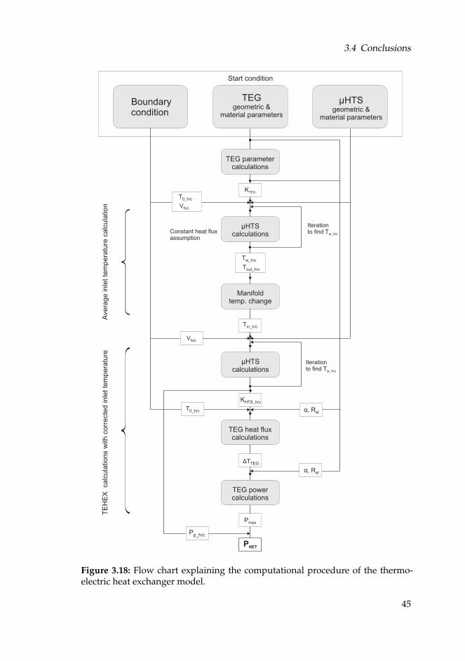
3.4 Conclusions
Boundarycondition
TEGgeometric &
material parameters
µHTSgeometric &
material parameters
Start condition
KTEG
TEG parametercalculations
T0_h/c
Vh/c
µHTScalculations
Iterationto find Tw_h/c
Tw_h/c
Tout_h/c
Constant heat fluxassumption
Manifoldtemp. change
µHTScalculations
Tin_h/c
Vh/c
KHTS_h/c
TEG heat fluxcalculations
ΔTTEG
TEG powercalculations
α, Rel
Pmax
PNET
Pp_h/c
Avera
ge inle
t te
mpera
ture
calc
ula
tion
TE
HE
X calc
ula
tions w
ith c
orr
ecte
d inle
t te
mpera
ture
α, Rel
Iterationto find Tw_h/c
T0_h/c
Figure 3.18: Flow chart explaining the computational procedure of the thermo-electric heat exchanger model.
45
3 Theory and Modelling
impacts of the reduced thermal contact resistances on the TEG performance aswell as important parameter correlations are discussed. Moreover, the reducedrelevance of the thermal conductivity in the thermoelectric material with decreas-ing contact resistances is highlighted.The existing thermal and hydrodynamic µHTS is extended with a discrete tem-perature profile inside the microchannels in order to account for the influenceof temperature dependent fluid parameters as well as to correctly model thegradual fluid temperature change along the manifold channels. This extensionsignificantly improves the agreement between measurements and model, in par-ticular for the thermal performance at lower fluid flow rates.Investigations on the improvement of the µHTS design by means of a 3D-FEMunit cell model yield an overall system performance enhancement by introducinghigh aspect ratio pin-fin structures and implementing a smoother fluid flow path.Finally, the iterative computational procedure of the combined TEHEX model isdescribed and reveals the necessary complexity for accurate system modelling.
46
4 Fabrication and Experimental
The small and large size TEGs used for the measurements are provided by green-TEG AG and are fabricated and characterized according to [28]. The fabricationof the corresponding 8 x 8 mm and 9 x 9 cm µHTSs are described in the first partof this chapter. In the second part, the experimental settings are explained.
4.1 Thermoelectric heat exchanger fabrication
For the fabrication of the small and large size µHTSs, two different approachesare used. The objective of the small µHTS is to develop a high performance sys-tem featuring high aspect ratio microchannels in order to demonstrate the tech-nological feasibility and limits of the thermoelectric heat exchanger. The focus ofthe large size fabrication is set on a straight forward, fast and reliable process inperspective of future commercialization.
4.1.1 Small size micro heat transfer system
1The two functional layers of the µHTS, the microchannel and the manifold struc-ture are fabricated in separate processes and assembled on chip level.
Microchannel fabrication
The microchannels are fabricated by means of SU-8 based high aspect ratio pho-tolithography and subsequent electrochemical deposition. The detailed processflow is illustrated in Figure 4.1. In the first step, 1µm of Lift-Off resist (LOR) isspin coated on the wafer for a later release of the microchannels from the sup-port. Next, a copper seed layer (1µm) and a chromium adhesion layer (10 nm)are deposited by e-beam evaporation (Fig. 4.1 a)). The prepared seed wafer iscoated with a 200µm thick SU-8 3050 film. To improve the layer thickness ho-mogeneity, the spin coating is performed in two steps of 100µm with an edgebead removal by γ-butyrolactone (GBL) after each step. In the subsequent pho-tolithography (Fig. 4.1 b)), reduced baking temperatures as well as long coolingand additional relaxation times are applied for stress reduction in the SU-8. Dueto the high aspect ratio and extended length of the mold structures, a reduced
1 The main content of the small microchannel fabrication process was published in [153] and wasreproduced with permission. Copyright c© 2012 Elsevier B.V.
47
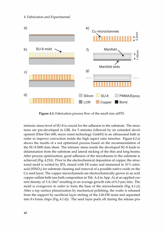
4 Fabrication and Experimental
Silicon
a)
c)
b)
g)
SU-8
CopperLOR Bond
0.2
mm
SU-8 mold
Cu microchannels
Manifold slots
d)
e)
PMMA/Epoxy
f)
1.4
5m
m
Manifold
Figure 4.1: Fabrication process flow of the small size µHTS.
intrinsic stress level of SU-8 is crucial for the adhesion to the substrate. The struc-tures are pre-developed in GBL for 5 minutes followed by an extended devel-opment (Dmr-Dev 600, micro resist technology GmbH) in an ultrasound bath inorder to improve convection inside the high aspect ratio trenches. Figure 4.2 a)shows the results of a not optimized process based on the recommendation ofthe SU-8 3000 data sheet. The intrinsic stress inside the developed SU-8 leads todelamination from the substrate and lateral sticking of the thin and long beams.After process optimization, good adhesion of the microbeams to the substrate isachieved (Fig. 4.2 b)). Prior to the electrochemical deposition of copper, the struc-tured mold is wetted by IPA, rinsed with DI water and immersed in 10 % nitricacid (HNO3) for substrate cleaning and removal of a possible native oxide on theCu seed layer. The copper microchannels are electrochemically grown in an acidcopper sulfate bath (see bath composition in Tab. A.4 in App. A) at an applied cur-rent density of 3 A/dm2 resulting in an average growth rate of 0.3µm/min. Themold is overgrown in order to form the base of the microchannels (Fig. 4.1 c)).After a top surface planarization by mechanical polishing, the wafer is releasedfrom the support by sacrificial layer etching of the Lift-Off resist and separatedinto 8 x 8 mm chips (Fig. 4.1 d)). The seed layer peels off during the release pro-
48
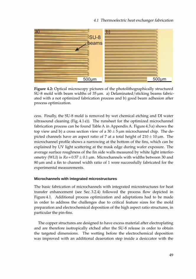
4.1 Thermoelectric heat exchanger fabrication
SU-8beams
a) b)
500µm500µm
Figure 4.2: Optical microscopy pictures of the photolithographically structuredSU-8 mold with beam widths of 35µm. a) Delaminated/sticking beams fabric-ated with a not optimized fabrication process and b) good beam adhesion afterprocess optimization.
cess. Finally, the SU-8 mold is removed by wet chemical etching and DI waterultrasound cleaning (Fig. 4.1 e)). The runsheet for the optimized microchannelfabrication process can be found Table A in Appendix A. Figure 4.3 a) shows thetop view and b) a cross section view of a 30± 5µm microchannel chip. The de-picted channels have an aspect ratio of 7 at a total height of 210± 10µm. Themicrochannel profile shows a narrowing at the bottom of the fins, which can beexplained by UV light scattering at the mask edge during wafer exposure. Theaverage surface roughness of the fin side walls measured by white light interfer-ometry (WLI) is Ra = 0.57± 0.1µm. Microchannels with widths between 30 and80µm and a fin to channel width ratio of 1 were successfully fabricated for theexperimental measurements.
Microchannels with integrated microstructures
The basic fabrication of microchannels with integrated microstructures for heattransfer enhancement (see Sec. 3.2.4) followed the process flow depicted inFigure 4.1. Additional process optimization and adaptations had to be madein order to address the challenges due to critical feature sizes for the moldpreparation and electrochemical deposition of the high aspect ratio structures, inparticular the pin-fins.
The copper structures are designed to have excess material after electroplatingand are therefore isotropically etched after the SU-8 release in order to obtainthe targeted dimensions. The wetting before the electrochemical depositionwas improved with an additional deaeration step inside a desiccator with the
49
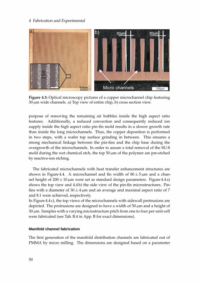
4 Fabrication and Experimental
30µm
Micro channels
b)a)
µm30
1mm
30µm
100µm
Figure 4.3: Optical microscopy pictures of a copper microchannel chip featuring30µm wide channels. a) Top view of entire chip, b) cross section view.
purpose of removing the remaining air bubbles inside the high aspect ratiofeatures. Additionally, a reduced convection and consequently reduced ionsupply inside the high aspect ratio pin-fin mold results in a slower growth ratethan inside the long microchannels. Thus, the copper deposition is performedin two steps, with a wafer top surface grinding in between. This ensures astrong mechanical linkage between the pin-fins and the chip base during theovergrowth of the microchannels. In order to assure a total removal of the SU-8mold during the wet chemical etch, the top 50µm of the polymer are pre-etchedby reactive-ion etching.
The fabricated microchannels with heat transfer enhancement structures areshown in Figure 4.4. A microchannel and fin width of 80± 5µm and a chan-nel height of 200± 10µm were set as standard design parameters. Figure 4.4 a)shows the top view and 4.4 b) the side view of the pin-fin microstructures. Pin-fins with a diameter of 30± 4µm and an average and maximal aspect ratio of 7and 8.1 were achieved, respectively.In Figure 4.4 c), the top views of the microchannels with sidewall protrusions aredepicted. The protrusions are designed to have a width of 50µm and a height of30µm. Samples with a varying microstructure pitch from one to four per unit-cellwere fabricated (see Tab. B.4 in App. B for exact dimensions).
Manifold channel fabrication
The first generation of the manifold distribution channels are fabricated out ofPMMA by micro milling. The dimensions are designed based on a parameter
50
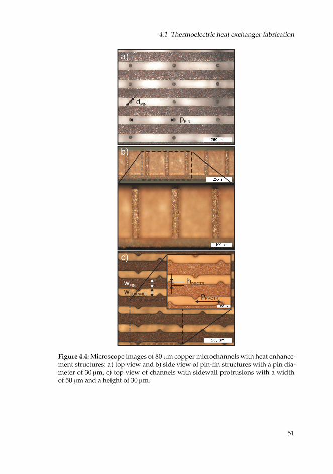
4.1 Thermoelectric heat exchanger fabrication
pPIN
dPIN
wFIN
wCHANNEL
a)
b)
c)
pPROTR
hPROTR
Figure 4.4: Microscope images of 80µm copper microchannels with heat enhance-ment structures: a) top view and b) side view of pin-fin structures with a pin dia-meter of 30µm, c) top view of channels with sidewall protrusions with a widthof 50µm and a height of 30µm.
51
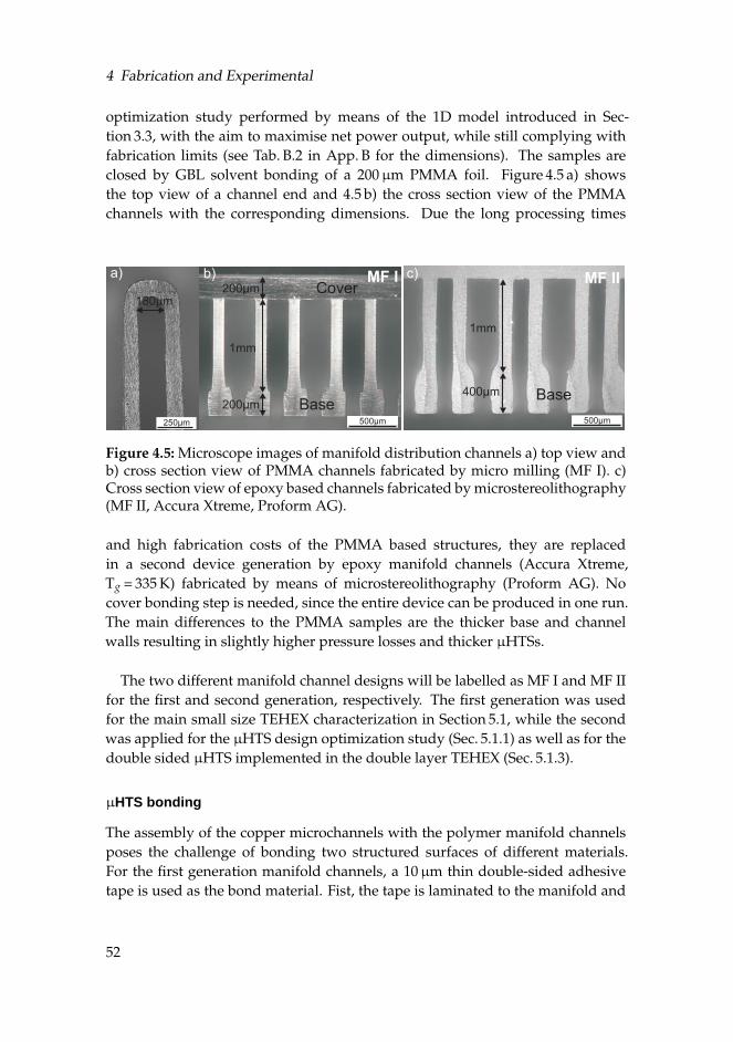
4 Fabrication and Experimental
optimization study performed by means of the 1D model introduced in Sec-tion 3.3, with the aim to maximise net power output, while still complying withfabrication limits (see Tab. B.2 in App. B for the dimensions). The samples areclosed by GBL solvent bonding of a 200µm PMMA foil. Figure 4.5 a) showsthe top view of a channel end and 4.5 b) the cross section view of the PMMAchannels with the corresponding dimensions. Due the long processing times
500µm
a) b) c)
Base
Cover200µm
200µm
1mm
400µm
1mm
Base
180µm
250µm 500µm
MF I MF II
Figure 4.5: Microscope images of manifold distribution channels a) top view andb) cross section view of PMMA channels fabricated by micro milling (MF I). c)Cross section view of epoxy based channels fabricated by microstereolithography(MF II, Accura Xtreme, Proform AG).
and high fabrication costs of the PMMA based structures, they are replacedin a second device generation by epoxy manifold channels (Accura Xtreme,Tg = 335 K) fabricated by means of microstereolithography (Proform AG). Nocover bonding step is needed, since the entire device can be produced in one run.The main differences to the PMMA samples are the thicker base and channelwalls resulting in slightly higher pressure losses and thicker µHTSs.
The two different manifold channel designs will be labelled as MF I and MF IIfor the first and second generation, respectively. The first generation was usedfor the main small size TEHEX characterization in Section 5.1, while the secondwas applied for the µHTS design optimization study (Sec. 5.1.1) as well as for thedouble sided µHTS implemented in the double layer TEHEX (Sec. 5.1.3).
µHTS bonding
The assembly of the copper microchannels with the polymer manifold channelsposes the challenge of bonding two structured surfaces of different materials.For the first generation manifold channels, a 10µm thin double-sided adhesivetape is used as the bond material. Fist, the tape is laminated to the manifold and
52
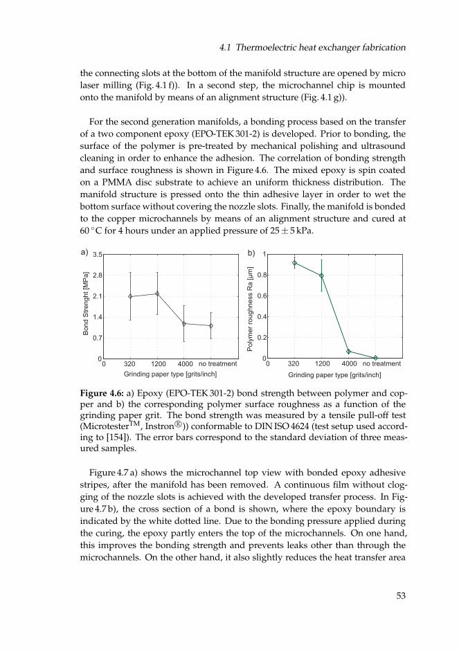
4.1 Thermoelectric heat exchanger fabrication
the connecting slots at the bottom of the manifold structure are opened by microlaser milling (Fig. 4.1 f)). In a second step, the microchannel chip is mountedonto the manifold by means of an alignment structure (Fig. 4.1 g)).
For the second generation manifolds, a bonding process based on the transferof a two component epoxy (EPO-TEK 301-2) is developed. Prior to bonding, thesurface of the polymer is pre-treated by mechanical polishing and ultrasoundcleaning in order to enhance the adhesion. The correlation of bonding strengthand surface roughness is shown in Figure 4.6. The mixed epoxy is spin coatedon a PMMA disc substrate to achieve an uniform thickness distribution. Themanifold structure is pressed onto the thin adhesive layer in order to wet thebottom surface without covering the nozzle slots. Finally, the manifold is bondedto the copper microchannels by means of an alignment structure and cured at60 C for 4 hours under an applied pressure of 25± 5 kPa.
0
0.7
1.4
2.1
2.8
3.5
Bo
nd
Str
en
gh
t [M
Pa
]
0 320 1200 4000 no treatment
Grinding paper type [grits/inch]
a)
0 320 1200 4000 no treatment0
0.2
0.4
0.6
0.8
1P
oly
me
r ro
ug
hn
ess R
a [
m]
μ
Grinding paper type [grits/inch]
b)
Figure 4.6: a) Epoxy (EPO-TEK 301-2) bond strength between polymer and cop-per and b) the corresponding polymer surface roughness as a function of thegrinding paper grit. The bond strength was measured by a tensile pull-off test(MicrotesterTM, Instron R©)) conformable to DIN ISO 4624 (test setup used accord-ing to [154]). The error bars correspond to the standard deviation of three meas-ured samples.
Figure 4.7 a) shows the microchannel top view with bonded epoxy adhesivestripes, after the manifold has been removed. A continuous film without clog-ging of the nozzle slots is achieved with the developed transfer process. In Fig-ure 4.7 b), the cross section of a bond is shown, where the epoxy boundary isindicated by the white dotted line. Due to the bonding pressure applied duringthe curing, the epoxy partly enters the top of the microchannels. On one hand,this improves the bonding strength and prevents leaks other than through themicrochannels. On the other hand, it also slightly reduces the heat transfer area
53
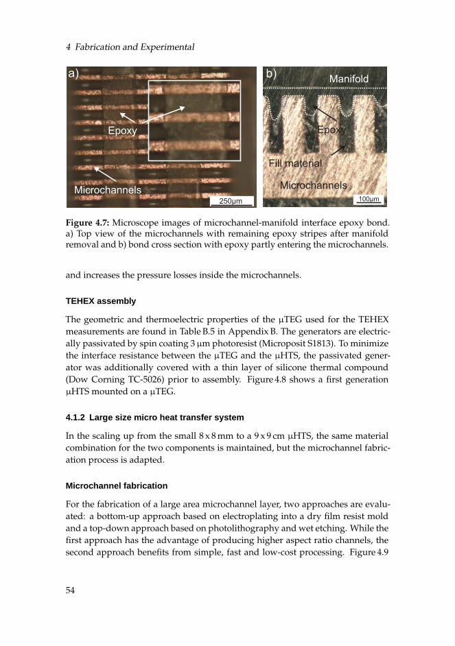
4 Fabrication and Experimental
a) b)
Epoxy
250µm 100µmMicrochannels
Epoxy
Manifold
Microchannels
Fill material
Figure 4.7: Microscope images of microchannel-manifold interface epoxy bond.a) Top view of the microchannels with remaining epoxy stripes after manifoldremoval and b) bond cross section with epoxy partly entering the microchannels.
and increases the pressure losses inside the microchannels.
TEHEX assembly
The geometric and thermoelectric properties of the µTEG used for the TEHEXmeasurements are found in Table B.5 in Appendix B. The generators are electric-ally passivated by spin coating 3µm photoresist (Microposit S1813). To minimizethe interface resistance between the µTEG and the µHTS, the passivated gener-ator was additionally covered with a thin layer of silicone thermal compound(Dow Corning TC-5026) prior to assembly. Figure 4.8 shows a first generationµHTS mounted on a µTEG.
4.1.2 Large size micro heat transfer system
In the scaling up from the small 8 x 8 mm to a 9 x 9 cm µHTS, the same materialcombination for the two components is maintained, but the microchannel fabric-ation process is adapted.
Microchannel fabrication
For the fabrication of a large area microchannel layer, two approaches are evalu-ated: a bottom-up approach based on electroplating into a dry film resist moldand a top-down approach based on photolithography and wet etching. While thefirst approach has the advantage of producing higher aspect ratio channels, thesecond approach benefits from simple, fast and low-cost processing. Figure 4.9
54
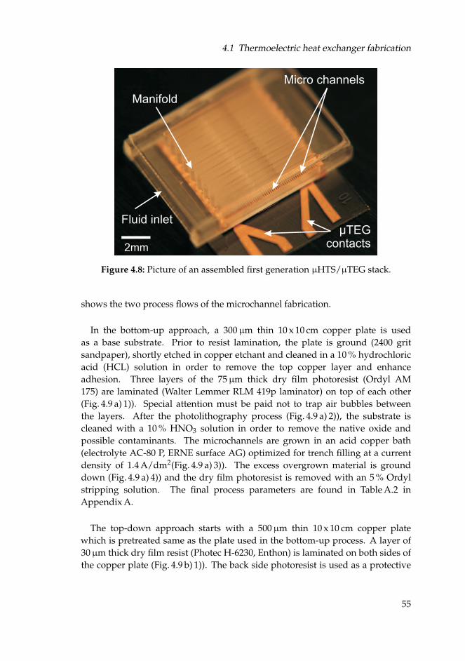
4.1 Thermoelectric heat exchanger fabrication
µTEGcontacts
Micro channels
2mm
Manifold
Fluid inlet
Figure 4.8: Picture of an assembled first generation µHTS/µTEG stack.
shows the two process flows of the microchannel fabrication.
In the bottom-up approach, a 300µm thin 10 x 10 cm copper plate is usedas a base substrate. Prior to resist lamination, the plate is ground (2400 gritsandpaper), shortly etched in copper etchant and cleaned in a 10 % hydrochloricacid (HCL) solution in order to remove the top copper layer and enhanceadhesion. Three layers of the 75µm thick dry film photoresist (Ordyl AM175) are laminated (Walter Lemmer RLM 419p laminator) on top of each other(Fig. 4.9 a) 1)). Special attention must be paid not to trap air bubbles betweenthe layers. After the photolithography process (Fig. 4.9 a) 2)), the substrate iscleaned with a 10 % HNO3 solution in order to remove the native oxide andpossible contaminants. The microchannels are grown in an acid copper bath(electrolyte AC-80 P, ERNE surface AG) optimized for trench filling at a currentdensity of 1.4 A/dm2(Fig. 4.9 a) 3)). The excess overgrown material is grounddown (Fig. 4.9 a) 4)) and the dry film photoresist is removed with an 5 % Ordylstripping solution. The final process parameters are found in Table A.2 inAppendix A.
The top-down approach starts with a 500µm thin 10 x 10 cm copper platewhich is pretreated same as the plate used in the bottom-up process. A layer of30µm thick dry film resist (Photec H-6230, Enthon) is laminated on both sides ofthe copper plate (Fig. 4.9 b) 1)). The back side photoresist is used as a protective
55
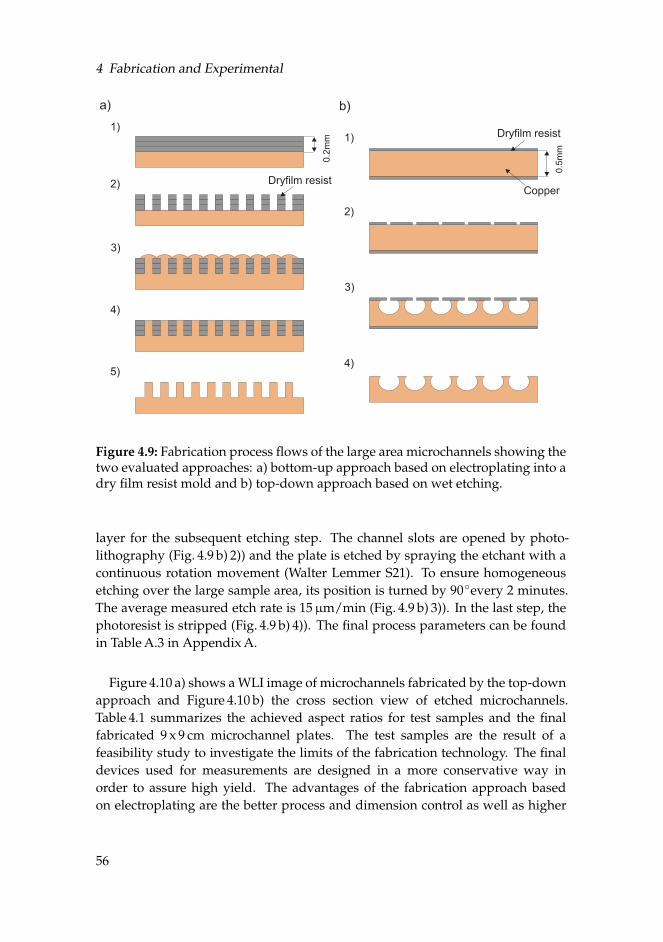
4 Fabrication and Experimental
1)
3)
2)
0.5
mm
4)
Dryfilm resist
Copper
1)
3)
2)
0.2
mm
4)
5)
b)a)
Dryfilm resist
Figure 4.9: Fabrication process flows of the large area microchannels showing thetwo evaluated approaches: a) bottom-up approach based on electroplating into adry film resist mold and b) top-down approach based on wet etching.
layer for the subsequent etching step. The channel slots are opened by photo-lithography (Fig. 4.9 b) 2)) and the plate is etched by spraying the etchant with acontinuous rotation movement (Walter Lemmer S21). To ensure homogeneousetching over the large sample area, its position is turned by 90every 2 minutes.The average measured etch rate is 15µm/min (Fig. 4.9 b) 3)). In the last step, thephotoresist is stripped (Fig. 4.9 b) 4)). The final process parameters can be foundin Table A.3 in Appendix A.
Figure 4.10 a) shows a WLI image of microchannels fabricated by the top-downapproach and Figure 4.10 b) the cross section view of etched microchannels.Table 4.1 summarizes the achieved aspect ratios for test samples and the finalfabricated 9 x 9 cm microchannel plates. The test samples are the result of afeasibility study to investigate the limits of the fabrication technology. The finaldevices used for measurements are designed in a more conservative way inorder to assure high yield. The advantages of the fabrication approach basedon electroplating are the better process and dimension control as well as higher
56
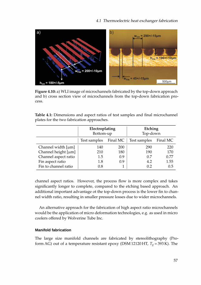
4.1 Thermoelectric heat exchanger fabrication
w = 45+/-15µmFIN
w = 290+/-15µmCH
h = 190+/-10µmCH
a) b)
500µm
w = 200+/-10µmFIN
h = 180+/-5µmCH
Figure 4.10: a) WLI image of microchannels fabricated by the top-down approachand b) cross section view of microchannels from the top-down fabrication pro-cess.
Table 4.1: Dimensions and aspect ratios of test samples and final microchannelplates for the two fabrication approaches.
Electroplating EtchingBottom-up Top-down
Test samples Final MC Test samples Final MC
Channel width [µm] 140 200 290 220Channel height [µm] 210 180 190 170Channel aspect ratio 1.5 0.9 0.7 0.77Fin aspect ratio 1.8 0.9 4.2 1.55Fin to channel ratio 0.8 1 0.2 0.5
channel aspect ratios. However, the process flow is more complex and takessignificantly longer to complete, compared to the etching based approach. Anadditional important advantage ot the top-down process is the lower fin to chan-nel width ratio, resulting in smaller pressure losses due to wider microchannels.
An alternative approach for the fabrication of high aspect ratio microchannelswould be the application of micro deformation technologies, e.g. as used in microcoolers offered by Wolverine Tube Inc.
Manifold fabrication
The large size manifold channels are fabricated by stereolithography (Pro-form AG) out of a temperature resistant epoxy (DSM 12120 HT, Tg = 393 K). The
57
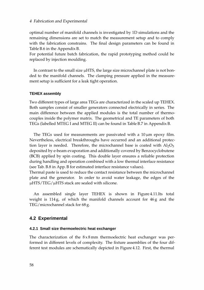
4 Fabrication and Experimental
optimal number of manifold channels is investigated by 1D simulations and theremaining dimensions are set to match the measurement setup and to complywith the fabrication constrains. The final design parameters can be found inTable B.6 in the Appendix B.For potential future batch fabrication, the rapid prototyping method could bereplaced by injection moulding.
In contrast to the small size µHTS, the large size microchannel plate is not bon-ded to the manifold channels. The clamping pressure applied in the measure-ment setup is sufficient for a leak tight operation.
TEHEX assembly
Two different types of large area TEGs are characterized in the scaled up TEHEX.Both samples consist of smaller generators connected electrically in series. Themain difference between the applied modules is the total number of thermo-couples inside the polymer matrix. The geometrical and TE parameters of bothTEGs (labelled MTEG I and MTEG II) can be found in Table B.7 in Appendix B.
The TEGs used for measurements are passivated with a 10µm epoxy film.Nevertheless, electrical breakthroughs have occurred and an additional protec-tion layer is needed. Therefore, the microchannel base is coated with Al2O3
deposited by e-beam evaporation and additionally covered by Benzocyclobutene(BCB) applied by spin coating. This double layer ensures a reliable protectionduring handling and operation combined with a low thermal interface resistance(see Tab. B.8 in App. B for estimated interface resistance values).Thermal paste is used to reduce the contact resistance between the microchannelplate and the generator. In order to avoid water leakage, the edges of theµHTS/TEG/µHTS stack are sealed with silicone.
An assembled single layer TEHEX is shown in Figure 4.11.Its totalweight is 114 g, of which the manifold channels account for 46 g and theTEG/microchannel stack for 68 g.
4.2 Experimental
4.2.1 Small size thermoelectric heat exchanger
The characterization of the 8 x 8 mm thermoelectric heat exchanger was per-formed in different levels of complexity. The fixture assemblies of the four dif-ferent test modules are schematically depicted in Figure 4.12. First, the thermal
58
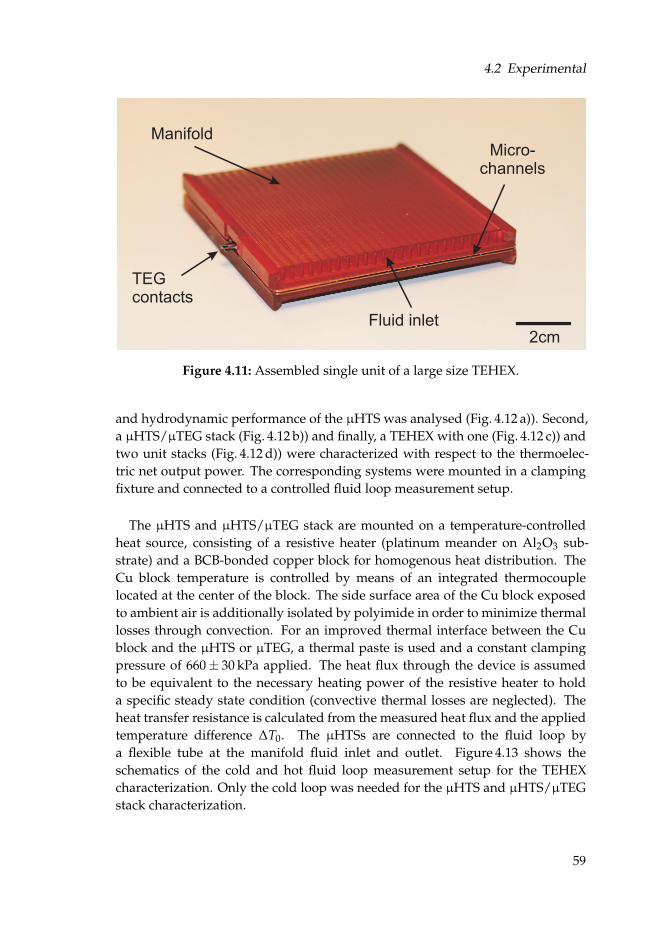
4.2 Experimental
TEGcontacts
Micro-channels
2cm
Manifold
Fluid inlet
Figure 4.11: Assembled single unit of a large size TEHEX.
and hydrodynamic performance of the µHTS was analysed (Fig. 4.12 a)). Second,a µHTS/µTEG stack (Fig. 4.12 b)) and finally, a TEHEX with one (Fig. 4.12 c)) andtwo unit stacks (Fig. 4.12 d)) were characterized with respect to the thermoelec-tric net output power. The corresponding systems were mounted in a clampingfixture and connected to a controlled fluid loop measurement setup.
The µHTS and µHTS/µTEG stack are mounted on a temperature-controlledheat source, consisting of a resistive heater (platinum meander on Al2O3 sub-strate) and a BCB-bonded copper block for homogenous heat distribution. TheCu block temperature is controlled by means of an integrated thermocouplelocated at the center of the block. The side surface area of the Cu block exposedto ambient air is additionally isolated by polyimide in order to minimize thermallosses through convection. For an improved thermal interface between the Cublock and the µHTS or µTEG, a thermal paste is used and a constant clampingpressure of 660± 30 kPa applied. The heat flux through the device is assumedto be equivalent to the necessary heating power of the resistive heater to holda specific steady state condition (convective thermal losses are neglected). Theheat transfer resistance is calculated from the measured heat flux and the appliedtemperature difference ∆T0. The µHTSs are connected to the fluid loop bya flexible tube at the manifold fluid inlet and outlet. Figure 4.13 shows theschematics of the cold and hot fluid loop measurement setup for the TEHEXcharacterization. Only the cold loop was needed for the µHTS and µHTS/µTEGstack characterization.
59
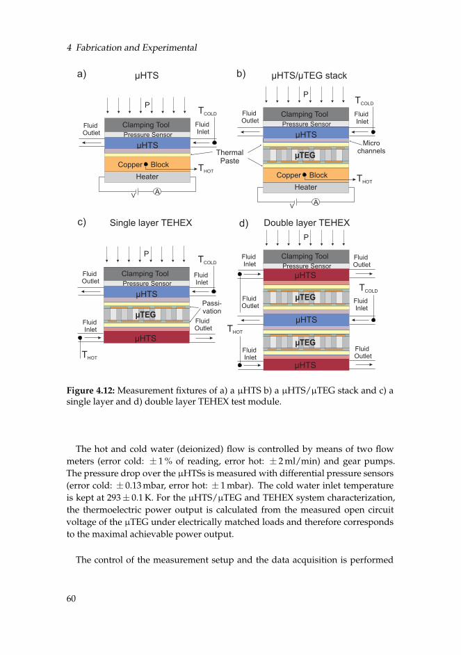
4 Fabrication and Experimental
THOT
Copper Block
A
Heater
ThermalPaste
P
µHTS
V
FluidInlet
FluidOutlet
Passi-vation
µTEG
TCOLD
Pressure Sensor
Clamping Tool
THOT
Copper Block
A
Heater
P
µHTS
V
FluidInlet
FluidOutlet
TCOLD
Pressure Sensor
Clamping Tool
THOT
P
FluidInlet
FluidOutlet
µTEG
TCOLD
Pressure Sensor
Clamping Tool
µHTS
µHTS
a) b)
c)
FluidOutlet
FluidInlet
µHTS µHTS/µTEG stack
Single layer TEHEX
THOT
P
FluidInlet
FluidOutlet
µTEG
TCOLD
Pressure Sensor
Clamping Tool
µHTS
µHTS
d)
FluidOutlet
FluidInlet
Double layer TEHEX
Microchannels
µTEG
µHTS
FluidOutlet
FluidInlet
Figure 4.12: Measurement fixtures of a) a µHTS b) a µHTS/µTEG stack and c) asingle layer and d) double layer TEHEX test module.
The hot and cold water (deionized) flow is controlled by means of two flowmeters (error cold: ± 1 % of reading, error hot: ± 2 ml/min) and gear pumps.The pressure drop over the µHTSs is measured with differential pressure sensors(error cold: ± 0.13 mbar, error hot: ± 1 mbar). The cold water inlet temperatureis kept at 293± 0.1 K. For the µHTS/µTEG and TEHEX system characterization,the thermoelectric power output is calculated from the measured open circuitvoltage of the µTEG under electrically matched loads and therefore correspondsto the maximal achievable power output.
The control of the measurement setup and the data acquisition is performed
60
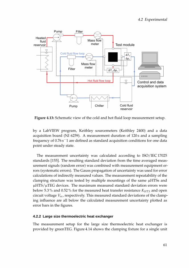
4.2 Experimental
Pump Chiller Cold fluidreservoir
Control and dataacquisition system
Filter
Mass flowmeter
Test module
ΔT ,ΔpC C
ΔT
ΔpH
H
Heatedfluid
reservoir
Filter
Mass flowmeter
Pump
Hot fluid flow loop
Cold fluid flow loop
Figure 4.13: Schematic view of the cold and hot fluid loop measurement setup.
by a LabVIEW program, Keithley sourcemeters (Keithley 2400) and a dataacquisition board (NI 6259). A measurement duration of 120 s and a samplingfrequency of 0.76 s−1 are defined as standard acquisition conditions for one datapoint under steady state.
The measurement uncertainty was calculated according to ISO/IEC 17025standards [155]. The resulting standard deviation from the time averaged meas-urement signals (random error) was combined with measurement equipment er-rors (systematic errors). The Gauss propagation of uncertainty was used for errorcalculations of indirectly measured values. The measurement repeatability of theclamping structure was tested by multiple mountings of the same µHTSs andµHTS/µTEG devices. The maximum measured standard deviation errors werebelow 5.3 % and 0.52 % for the measured heat transfer resistance KHTS and opencircuit voltage Voc, respectively. This measured standard deviations of the clamp-ing influence are all below the calculated measurement uncertainty plotted aserror bars in the figures.
4.2.2 Large size thermoelectric heat exchanger
The measurement setup for the large size thermoelectric heat exchanger isprovided by greenTEG. Figure 4.14 shows the clamping fixture for a single unit
61
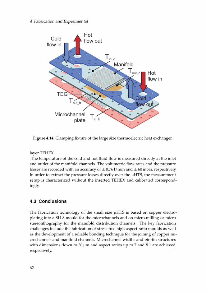
4 Fabrication and Experimental
Manifold
Tin_c
Microchannelplate
Hotflow in
Hotflow outCold
flow in
Coldflow out
Tout_c
Tin_h
Tout_h
TEG
Figure 4.14: Clamping fixture of the large size thermoelectric heat exchanger.
layer TEHEX.The temperature of the cold and hot fluid flow is measured directly at the inlet
and outlet of the manifold channels. The volumetric flow rates and the pressurelosses are recorded with an accuracy of ± 0.76 l/min and ± 60 mbar, respectively.In order to extract the pressure losses directly over the µHTS, the measurementsetup is characterized without the inserted TEHEX and calibrated correspond-ingly.
4.3 Conclusions
The fabrication technology of the small size µHTS is based on copper electro-plating into a SU-8 mould for the microchannels and on micro milling or microstereolithography for the manifold distribution channels. The key fabricationchallenges include the fabrication of stress free high aspect ratio moulds as wellas the development of a reliable bonding technique for the joining of copper mi-crochannels and manifold channels. Microchannel widths and pin-fin structureswith dimensions down to 30µm and aspect ratios up to 7 and 8.1 are achieved,respectively.
62

4.3 Conclusions
For the scaled up device, two fabrication approaches are evaluated and com-pared: a bottom-up approach similar to the small size fabrication process basedon electroplating and a top-down approach based on photolithography and etch-ing. With the first approach, higher aspect ratio channels are feasible, while thesecond method benefits from fast and simple processing as well as low fin tochannel ratios and is thus selected for device implementation.The assembled small and large size devices are mounted in corresponding clamp-ing structures and characterized in controlled fluid loop measurement setups.
63

5 Device Characterisation
Many different sets of parameters influence the performance of the thermoelec-tric heat exchanger; namely the dimensions of the µHTS itself, the properties anddimensions of the thermoelectric generator as well as the applied boundary orworking conditions.
The 8 x 8 mm systems are used to investigate and understand the different para-meter dependencies with the aim of optimizing the overall system’s net outputperformance. The goal of the large 9 x 9 cm TEHEX is to show the feasibility of thedevice upscaling and to demonstrate its potential for large scale low temperaturewaste heat recovery.
5.1 Small size thermoelectric heat exchanger
1This section focuses on the investigation and characterization of the most import-ant TEHEX system parameters. For this purpose, the complex system is dividedinto individual subsystems. In the first part, the µHTS itself is characterized withrespect to the system’s dimensions, flow rates and applied temperature gradi-ents. In the second part, the output performance of the µHTS/µTEG systemsis analysed with regard to the microchannel dimensions of the µHTS, boundaryconditions, µTEG thermal resistance and thermoelectric properties. In the lastsection, a complete TEHEX consisting of one and two unit cells is studied. Theadvantages of variable thermal resistances are discussed and practical aspects ofthermal resistance matching are evaluated.
5.1.1 Micro heat transfer system
Figure 5.1 shows the measured and computed thermal and hydrodynamicperformance of µHTSs with different microchannel widths relative to the fluidflow rate. Figure 5.1 a) depicts the removed heat flux and Figure 5.1 b) shows thecorresponding heat transfer resistance KHTS. The heat flux increases stronglywith increasing flow rates, mainly due to the corresponding rise in the heatcapacity rate of the fluid. However, towards higher flow rates, the influenceof the increasing mass flow on the heat flux is limited by the convective heattransfer. With decreasing channel widths, the heat flux is enhanced mainly due
1 The results of the µHTS and µHTS/µTEG system were published in [156] and were reproducedwith permission. Copyright c© 2013 Elsevier B.V.
65
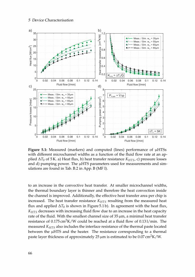
5 Device Characterisation
b)
P = VPUMP Dp
a)
c) d)
DT = 5K0
K = T /QHTS 0D
Meas. / Sim. w = 35µmch
Meas. / Sim. w = 50µm
Meas. / Sim. w = 60µm
Meas. / Sim. w = 80µm
ch
ch
ch
Meas. / Sim. w = 35µmch
Meas. / Sim. w = 50µm
Meas. / Sim. w = 60µm
Meas. / Sim. w = 80µm
ch
ch
ch
Heat tr
ansfe
r re
sis
tance
Figure 5.1: Measured (markers) and computed (lines) performance of µHTSswith different microchannel widths as a function of the fluid flow rate at an ap-plied ∆T0 of 5 K. a) Heat flux, b) heat transfer resistance KHTS, c) pressure lossesand d) pumping power. The µHTS parameters used for measurements and sim-ulations are found in Tab. B.2 in App. B (MF I).
to an increase in the convective heat transfer. At smaller microchannel widths,the thermal boundary layer is thinner and therefore the heat convection insidethe channel is improved. Additionally, the effective heat transfer area per chip isincreased. The heat transfer resistance KHTS resulting from the measured heatflux and applied ∆T0 is shown in Figure 5.1 b). In agreement with the heat flux,KHTS decreases with increasing fluid flow due to an increase in the heat capacityrate of the fluid. With the smallest channel size of 35µm, a minimal heat transferresistance of 0.175 cm2K/W could be reached at a fluid flow of 0.13 l/min. Themeasured KHTS also includes the interface resistance of the thermal paste locatedbetween the µHTS and the heater. The resistance corresponding to a thermalpaste layer thickness of approximately 25µm is estimated to be 0.07 cm2K/W.
66
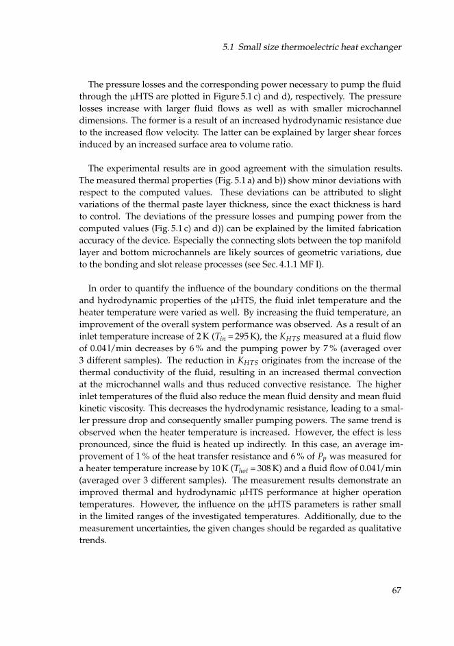
5.1 Small size thermoelectric heat exchanger
The pressure losses and the corresponding power necessary to pump the fluidthrough the µHTS are plotted in Figure 5.1 c) and d), respectively. The pressurelosses increase with larger fluid flows as well as with smaller microchanneldimensions. The former is a result of an increased hydrodynamic resistance dueto the increased flow velocity. The latter can be explained by larger shear forcesinduced by an increased surface area to volume ratio.
The experimental results are in good agreement with the simulation results.The measured thermal properties (Fig. 5.1 a) and b)) show minor deviations withrespect to the computed values. These deviations can be attributed to slightvariations of the thermal paste layer thickness, since the exact thickness is hardto control. The deviations of the pressure losses and pumping power from thecomputed values (Fig. 5.1 c) and d)) can be explained by the limited fabricationaccuracy of the device. Especially the connecting slots between the top manifoldlayer and bottom microchannels are likely sources of geometric variations, dueto the bonding and slot release processes (see Sec. 4.1.1 MF I).
In order to quantify the influence of the boundary conditions on the thermaland hydrodynamic properties of the µHTS, the fluid inlet temperature and theheater temperature were varied as well. By increasing the fluid temperature, animprovement of the overall system performance was observed. As a result of aninlet temperature increase of 2 K (Tin = 295 K), the KHTS measured at a fluid flowof 0.04 l/min decreases by 6 % and the pumping power by 7 % (averaged over3 different samples). The reduction in KHTS originates from the increase of thethermal conductivity of the fluid, resulting in an increased thermal convectionat the microchannel walls and thus reduced convective resistance. The higherinlet temperatures of the fluid also reduce the mean fluid density and mean fluidkinetic viscosity. This decreases the hydrodynamic resistance, leading to a smal-ler pressure drop and consequently smaller pumping powers. The same trend isobserved when the heater temperature is increased. However, the effect is lesspronounced, since the fluid is heated up indirectly. In this case, an average im-provement of 1 % of the heat transfer resistance and 6 % of Pp was measured fora heater temperature increase by 10 K (Thot = 308 K) and a fluid flow of 0.04 l/min(averaged over 3 different samples). The measurement results demonstrate animproved thermal and hydrodynamic µHTS performance at higher operationtemperatures. However, the influence on the µHTS parameters is rather smallin the limited ranges of the investigated temperatures. Additionally, due to themeasurement uncertainties, the given changes should be regarded as qualitativetrends.
67
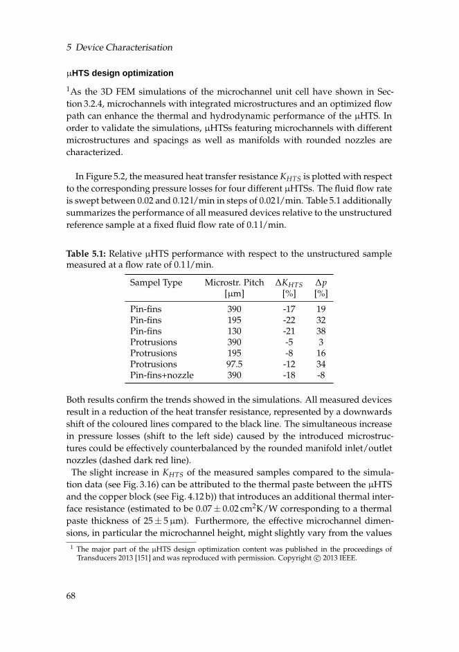
5 Device Characterisation
µHTS design optimization
1As the 3D FEM simulations of the microchannel unit cell have shown in Sec-tion 3.2.4, microchannels with integrated microstructures and an optimized flowpath can enhance the thermal and hydrodynamic performance of the µHTS. Inorder to validate the simulations, µHTSs featuring microchannels with differentmicrostructures and spacings as well as manifolds with rounded nozzles arecharacterized.
In Figure 5.2, the measured heat transfer resistance KHTS is plotted with respectto the corresponding pressure losses for four different µHTSs. The fluid flow rateis swept between 0.02 and 0.12 l/min in steps of 0.02 l/min. Table 5.1 additionallysummarizes the performance of all measured devices relative to the unstructuredreference sample at a fixed fluid flow rate of 0.1 l/min.
Table 5.1: Relative µHTS performance with respect to the unstructured samplemeasured at a flow rate of 0.1 l/min.
Sampel Type Microstr. Pitch ∆KHTS ∆p[µm] [%] [%]
Pin-fins 390 -17 19Pin-fins 195 -22 32Pin-fins 130 -21 38Protrusions 390 -5 3Protrusions 195 -8 16Protrusions 97.5 -12 34Pin-fins+nozzle 390 -18 -8
Both results confirm the trends showed in the simulations. All measured devicesresult in a reduction of the heat transfer resistance, represented by a downwardsshift of the coloured lines compared to the black line. The simultaneous increasein pressure losses (shift to the left side) caused by the introduced microstruc-tures could be effectively counterbalanced by the rounded manifold inlet/outletnozzles (dashed dark red line).
The slight increase in KHTS of the measured samples compared to the simula-tion data (see Fig. 3.16) can be attributed to the thermal paste between the µHTSand the copper block (see Fig. 4.12 b)) that introduces an additional thermal inter-face resistance (estimated to be 0.07± 0.02 cm2K/W corresponding to a thermalpaste thickness of 25± 5µm). Furthermore, the effective microchannel dimen-sions, in particular the microchannel height, might slightly vary from the values
1 The major part of the µHTS design optimization content was published in the proceedings ofTransducers 2013 [151] and was reproduced with permission. Copyright c© 2013 IEEE.
68
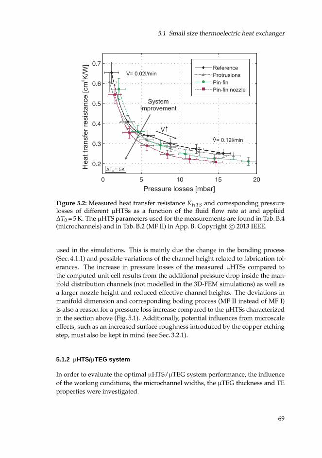
5.1 Small size thermoelectric heat exchanger
V= 0.02l/min
V= 0.12l/min
Reference
Protrusions
Pin-fin
Pin-fin nozzle
V
ΔT = 5K0
SystemImprovement
Pressure losses [mbar]
Heat tr
ansfe
r re
sis
tance [cm
K/W
]2
Figure 5.2: Measured heat transfer resistance KHTS and corresponding pressurelosses of different µHTSs as a function of the fluid flow rate at and applied∆T0 = 5 K. The µHTS parameters used for the measurements are found in Tab. B.4(microchannels) and in Tab. B.2 (MF II) in App. B. Copyright c© 2013 IEEE.
used in the simulations. This is mainly due the change in the bonding process(Sec. 4.1.1) and possible variations of the channel height related to fabrication tol-erances. The increase in pressure losses of the measured µHTSs compared tothe computed unit cell results from the additional pressure drop inside the man-ifold distribution channels (not modelled in the 3D-FEM simulations) as well asa larger nozzle height and reduced effective channel heights. The deviations inmanifold dimension and corresponding boding process (MF II instead of MF I)is also a reason for a pressure loss increase compared to the µHTSs characterizedin the section above (Fig. 5.1). Additionally, potential influences from microscaleeffects, such as an increased surface roughness introduced by the copper etchingstep, must also be kept in mind (see Sec. 3.2.1).
5.1.2 µHTS/µTEG system
In order to evaluate the optimal µHTS/µTEG system performance, the influenceof the working conditions, the microchannel widths, the µTEG thickness and TEproperties were investigated.
69
5 Device Characterisation
Influence of working conditions
Figure 5.3 a) shows the measured Seebeck voltage and the output power ofthe µHTS/µTEG system with respect to the applied temperature gradient anddifferent fluid flow rates. In Figure 5.3 b), the corresponding net output power isdepicted. The slope of the Seebeck voltage (solid line) increases with increasingflow rates, i.e. decreasing heat transfer resistance KHTS, due to an increased
a)
b)
P =NET P - PTEG PUMP
1
2
0
0
ZT = 0.047
PF = 1.4E-5 W/Km
m2
V = 0.02 l/min, K = 0.48 cm K/WHTS
2
V = 0.04 l/min, K = 0.24 cm K/W
V = 0.07 l/min, K = 0.14 cm K/W
V = 0.10 l/min, K = 0.11 cm K/W
HTS
HTS
HTS
2
2
2
w = 35 µmch
Figure 5.3: a) Seebeck voltage (solid lines) and output power (dashed lines) meas-urements of the µHTS/µTEG system and b) net output power as a function ofthe applied ∆T0 and the fluid flow rate for wch = 35µm. The µTEG (STEG I) andµHTS (MF I) parameters used for measurements and simulations are found inTab. B.5 and Tab. B.2 in App. B, respectively.
70
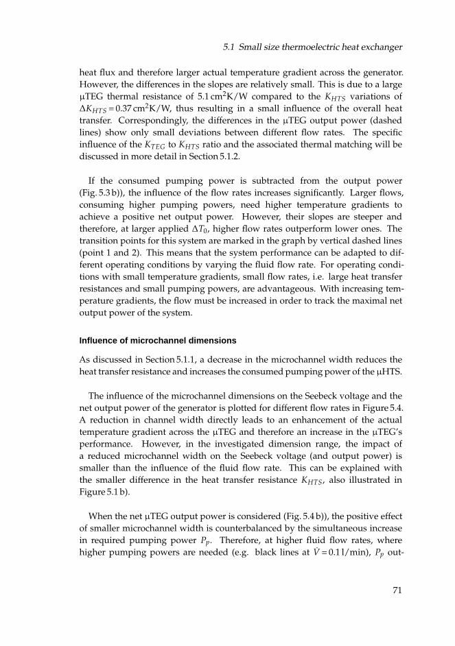
5.1 Small size thermoelectric heat exchanger
heat flux and therefore larger actual temperature gradient across the generator.However, the differences in the slopes are relatively small. This is due to a largeµTEG thermal resistance of 5.1 cm2K/W compared to the KHTS variations of∆KHTS = 0.37 cm2K/W, thus resulting in a small influence of the overall heattransfer. Correspondingly, the differences in the µTEG output power (dashedlines) show only small deviations between different flow rates. The specificinfluence of the KTEG to KHTS ratio and the associated thermal matching will bediscussed in more detail in Section 5.1.2.
If the consumed pumping power is subtracted from the output power(Fig. 5.3 b)), the influence of the flow rates increases significantly. Larger flows,consuming higher pumping powers, need higher temperature gradients toachieve a positive net output power. However, their slopes are steeper andtherefore, at larger applied ∆T0, higher flow rates outperform lower ones. Thetransition points for this system are marked in the graph by vertical dashed lines(point 1 and 2). This means that the system performance can be adapted to dif-ferent operating conditions by varying the fluid flow rate. For operating condi-tions with small temperature gradients, small flow rates, i.e. large heat transferresistances and small pumping powers, are advantageous. With increasing tem-perature gradients, the flow must be increased in order to track the maximal netoutput power of the system.
Influence of microchannel dimensions
As discussed in Section 5.1.1, a decrease in the microchannel width reduces theheat transfer resistance and increases the consumed pumping power of the µHTS.
The influence of the microchannel dimensions on the Seebeck voltage and thenet output power of the generator is plotted for different flow rates in Figure 5.4.A reduction in channel width directly leads to an enhancement of the actualtemperature gradient across the µTEG and therefore an increase in the µTEG’sperformance. However, in the investigated dimension range, the impact ofa reduced microchannel width on the Seebeck voltage (and output power) issmaller than the influence of the fluid flow rate. This can be explained withthe smaller difference in the heat transfer resistance KHTS, also illustrated inFigure 5.1 b).
When the net µTEG output power is considered (Fig. 5.4 b)), the positive effectof smaller microchannel width is counterbalanced by the simultaneous increasein required pumping power Pp. Therefore, at higher fluid flow rates, wherehigher pumping powers are needed (e.g. black lines at V = 0.1 l/min), Pp out-
71
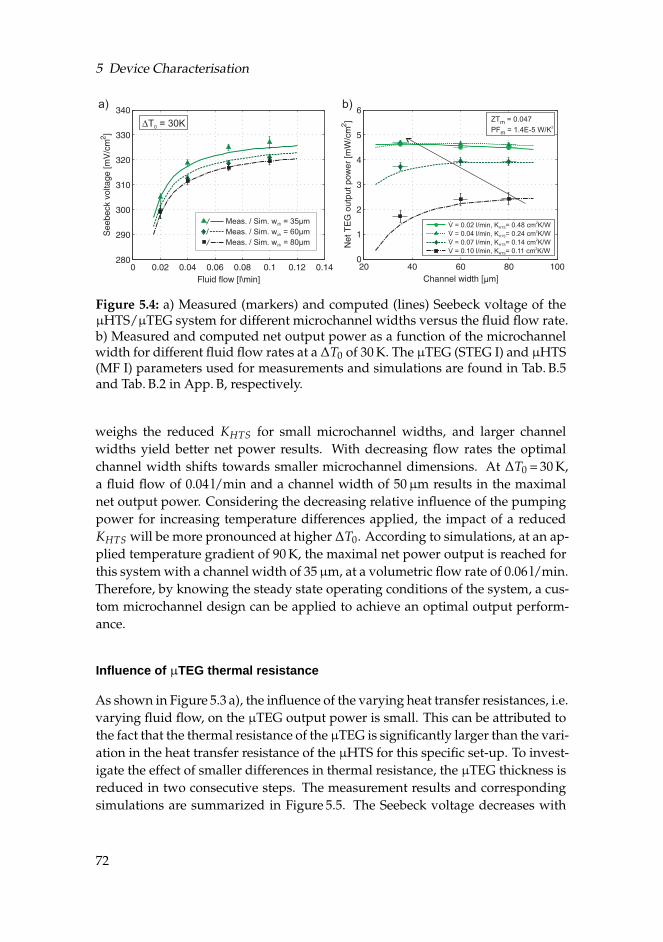
5 Device Characterisation
a) b)
DT = 30K0
V = 0.02 l/min, K = 0.48 cm K/WHTS
2
V = 0.04 l/min, K = 0.24 cm K/W
V = 0.07 l/min, K = 0.14 cm K/W
V = 0.10 l/min, K = 0.11 cm K/W
HTS
HTS
HTS
2
2
2
µ
Meas. / Sim. w = 35µmch
Meas. / Sim. w = 60µm
Meas. / Sim. w = 80µmch
ch
ZT = 0.047
PF = 1.4E-5 W/Km
m2
Figure 5.4: a) Measured (markers) and computed (lines) Seebeck voltage of theµHTS/µTEG system for different microchannel widths versus the fluid flow rate.b) Measured and computed net output power as a function of the microchannelwidth for different fluid flow rates at a ∆T0 of 30 K. The µTEG (STEG I) and µHTS(MF I) parameters used for measurements and simulations are found in Tab. B.5and Tab. B.2 in App. B, respectively.
weighs the reduced KHTS for small microchannel widths, and larger channelwidths yield better net power results. With decreasing flow rates the optimalchannel width shifts towards smaller microchannel dimensions. At ∆T0 = 30 K,a fluid flow of 0.04 l/min and a channel width of 50µm results in the maximalnet output power. Considering the decreasing relative influence of the pumpingpower for increasing temperature differences applied, the impact of a reducedKHTS will be more pronounced at higher ∆T0. According to simulations, at an ap-plied temperature gradient of 90 K, the maximal net power output is reached forthis system with a channel width of 35µm, at a volumetric flow rate of 0.06 l/min.Therefore, by knowing the steady state operating conditions of the system, a cus-tom microchannel design can be applied to achieve an optimal output perform-ance.
Influence of µTEG thermal resistance
As shown in Figure 5.3 a), the influence of the varying heat transfer resistances, i.e.varying fluid flow, on the µTEG output power is small. This can be attributed tothe fact that the thermal resistance of the µTEG is significantly larger than the vari-ation in the heat transfer resistance of the µHTS for this specific set-up. To invest-igate the effect of smaller differences in thermal resistance, the µTEG thickness isreduced in two consecutive steps. The measurement results and correspondingsimulations are summarized in Figure 5.5. The Seebeck voltage decreases with
72
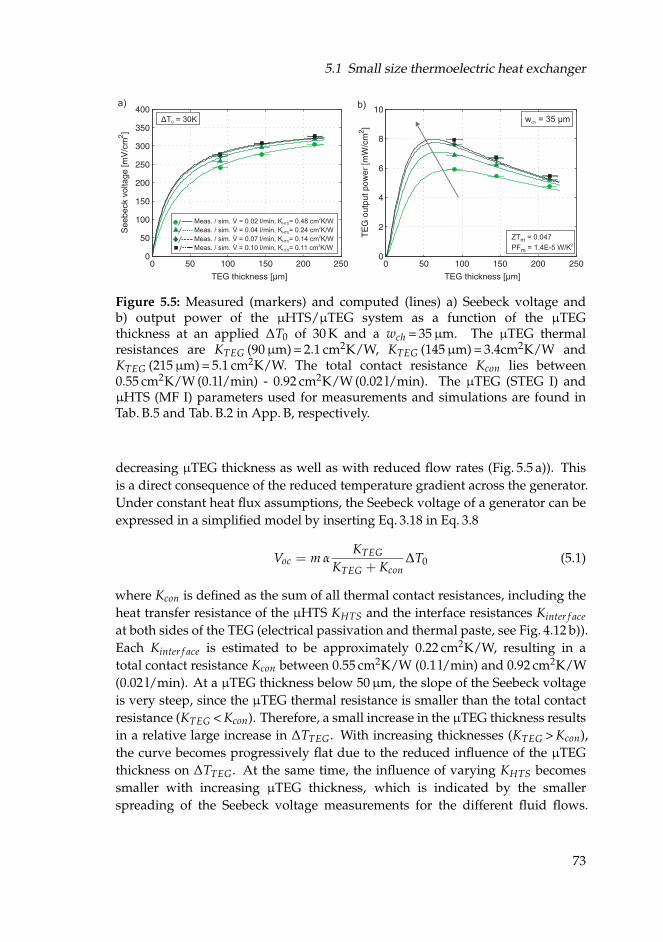
5.1 Small size thermoelectric heat exchanger
Meas. / sim.
Meas. / sim.
Meas. / sim.
Meas. / sim.
V = 0.02 l/min, K = 0.48 cm K/WHTS
2
V = 0.04 l/min, K = 0.24 cm K/W
V = 0.07 l/min, K = 0.14 cm K/W
V = 0.10 l/min, K = 0.11 cm K/W
HTS
HTS
HTS
2
2
2
b)a)
w = 35 µmchΔT = 30K0
ZT = 0.047
PF = 1.4E-5 W/Km
m2
TEG thickness [µm] TEG thickness [µm]
Figure 5.5: Measured (markers) and computed (lines) a) Seebeck voltage andb) output power of the µHTS/µTEG system as a function of the µTEGthickness at an applied ∆T0 of 30 K and a wch = 35µm. The µTEG thermalresistances are KTEG (90µm) = 2.1 cm2K/W, KTEG (145µm) = 3.4cm2K/W andKTEG (215µm) = 5.1 cm2K/W. The total contact resistance Kcon lies between0.55 cm2K/W (0.1l/min) - 0.92 cm2K/W (0.02 l/min). The µTEG (STEG I) andµHTS (MF I) parameters used for measurements and simulations are found inTab. B.5 and Tab. B.2 in App. B, respectively.
decreasing µTEG thickness as well as with reduced flow rates (Fig. 5.5 a)). Thisis a direct consequence of the reduced temperature gradient across the generator.Under constant heat flux assumptions, the Seebeck voltage of a generator can beexpressed in a simplified model by inserting Eq. 3.18 in Eq. 3.8
Voc = m αKTEG
KTEG + Kcon∆T0 (5.1)
where Kcon is defined as the sum of all thermal contact resistances, including theheat transfer resistance of the µHTS KHTS and the interface resistances Kinter f ace
at both sides of the TEG (electrical passivation and thermal paste, see Fig. 4.12 b)).Each Kinter f ace is estimated to be approximately 0.22 cm2K/W, resulting in atotal contact resistance Kcon between 0.55 cm2K/W (0.1 l/min) and 0.92 cm2K/W(0.02 l/min). At a µTEG thickness below 50µm, the slope of the Seebeck voltageis very steep, since the µTEG thermal resistance is smaller than the total contactresistance (KTEG < Kcon). Therefore, a small increase in the µTEG thickness resultsin a relative large increase in ∆TTEG. With increasing thicknesses (KTEG > Kcon),the curve becomes progressively flat due to the reduced influence of the µTEGthickness on ∆TTEG. At the same time, the influence of varying KHTS becomessmaller with increasing µTEG thickness, which is indicated by the smallerspreading of the Seebeck voltage measurements for the different fluid flows.
73
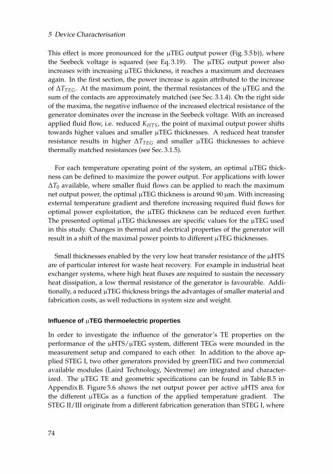
5 Device Characterisation
This effect is more pronounced for the µTEG output power (Fig. 5.5 b)), wherethe Seebeck voltage is squared (see Eq. 3.19). The µTEG output power alsoincreases with increasing µTEG thickness, it reaches a maximum and decreasesagain. In the first section, the power increase is again attributed to the increaseof ∆TTEG. At the maximum point, the thermal resistances of the µTEG and thesum of the contacts are approximately matched (see Sec. 3.1.4). On the right sideof the maxima, the negative influence of the increased electrical resistance of thegenerator dominates over the increase in the Seebeck voltage. With an increasedapplied fluid flow, i.e. reduced KHTS, the point of maximal output power shiftstowards higher values and smaller µTEG thicknesses. A reduced heat transferresistance results in higher ∆TTEG and smaller µTEG thicknesses to achievethermally matched resistances (see Sec. 3.1.5).
For each temperature operating point of the system, an optimal µTEG thick-ness can be defined to maximize the power output. For applications with lower∆T0 available, where smaller fluid flows can be applied to reach the maximumnet output power, the optimal µTEG thickness is around 90µm. With increasingexternal temperature gradient and therefore increasing required fluid flows foroptimal power exploitation, the µTEG thickness can be reduced even further.The presented optimal µTEG thicknesses are specific values for the µTEG usedin this study. Changes in thermal and electrical properties of the generator willresult in a shift of the maximal power points to different µTEG thicknesses.
Small thicknesses enabled by the very low heat transfer resistance of the µHTSare of particular interest for waste heat recovery. For example in industrial heatexchanger systems, where high heat fluxes are required to sustain the necessaryheat dissipation, a low thermal resistance of the generator is favourable. Addi-tionally, a reduced µTEG thickness brings the advantages of smaller material andfabrication costs, as well reductions in system size and weight.
Influence of µTEG thermoelectric properties
In order to investigate the influence of the generator’s TE properties on theperformance of the µHTS/µTEG system, different TEGs were mounded in themeasurement setup and compared to each other. In addition to the above ap-plied STEG I, two other generators provided by greenTEG and two commercialavailable modules (Laird Technology, Nextreme) are integrated and character-ized. The µTEG TE and geometric specifications can be found in Table B.5 inAppendix B. Figure 5.6 shows the net output power per active µHTS area forthe different µTEGs as a function of the applied temperature gradient. TheSTEG II/III originate from a different fabrication generation than STEG I, where
74
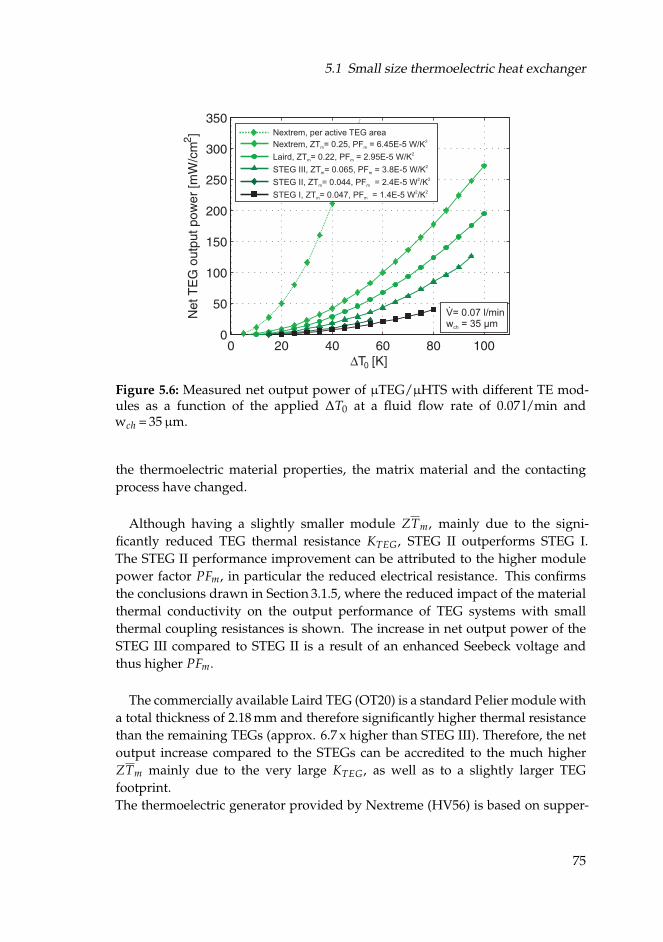
5.1 Small size thermoelectric heat exchanger
V=w = 35 µm
0.07 l/min
ch
0
2
2
2
2 2
2 2
Nextrem, per active TEG area
Nextrem, ZT = 0.25, PF = 6.45E-5 W/K
Laird, ZT = 0.22, PF = 2.95E-5 W/K
K
STEG II, ZT = 0.044, PF = 2.4E-5 W /K
STEG I, ZT = 0.047, PF = 1.4E-5 W /K
m m
m m
m
m m
m m
STEG III, ZT = 0.065, PF = 3.8E-5 W/m
Figure 5.6: Measured net output power of µTEG/µHTS with different TE mod-ules as a function of the applied ∆T0 at a fluid flow rate of 0.07 l/min andwch = 35µm.
the thermoelectric material properties, the matrix material and the contactingprocess have changed.
Although having a slightly smaller module ZTm, mainly due to the signi-ficantly reduced TEG thermal resistance KTEG, STEG II outperforms STEG I.The STEG II performance improvement can be attributed to the higher modulepower factor PFm, in particular the reduced electrical resistance. This confirmsthe conclusions drawn in Section 3.1.5, where the reduced impact of the materialthermal conductivity on the output performance of TEG systems with smallthermal coupling resistances is shown. The increase in net output power of theSTEG III compared to STEG II is a result of an enhanced Seebeck voltage andthus higher PFm.
The commercially available Laird TEG (OT20) is a standard Pelier module witha total thickness of 2.18 mm and therefore significantly higher thermal resistancethan the remaining TEGs (approx. 6.7 x higher than STEG III). Therefore, the netoutput increase compared to the STEGs can be accredited to the much higherZTm mainly due to the very large KTEG, as well as to a slightly larger TEGfootprint.The thermoelectric generator provided by Nextreme (HV56) is based on supper-
75
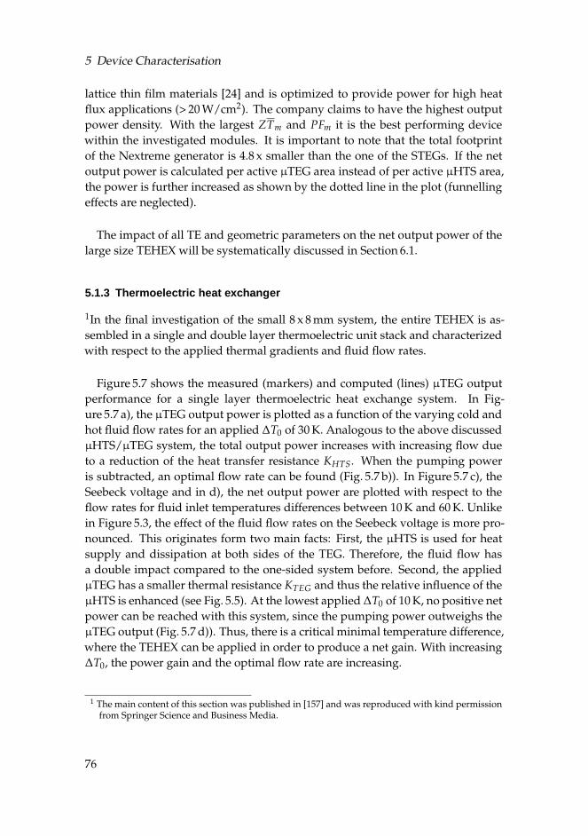
5 Device Characterisation
lattice thin film materials [24] and is optimized to provide power for high heatflux applications (> 20 W/cm2). The company claims to have the highest outputpower density. With the largest ZTm and PFm it is the best performing devicewithin the investigated modules. It is important to note that the total footprintof the Nextreme generator is 4.8 x smaller than the one of the STEGs. If the netoutput power is calculated per active µTEG area instead of per active µHTS area,the power is further increased as shown by the dotted line in the plot (funnellingeffects are neglected).
The impact of all TE and geometric parameters on the net output power of thelarge size TEHEX will be systematically discussed in Section 6.1.
5.1.3 Thermoelectric heat exchanger
1In the final investigation of the small 8 x 8 mm system, the entire TEHEX is as-sembled in a single and double layer thermoelectric unit stack and characterizedwith respect to the applied thermal gradients and fluid flow rates.
Figure 5.7 shows the measured (markers) and computed (lines) µTEG outputperformance for a single layer thermoelectric heat exchange system. In Fig-ure 5.7 a), the µTEG output power is plotted as a function of the varying cold andhot fluid flow rates for an applied ∆T0 of 30 K. Analogous to the above discussedµHTS/µTEG system, the total output power increases with increasing flow dueto a reduction of the heat transfer resistance KHTS. When the pumping poweris subtracted, an optimal flow rate can be found (Fig. 5.7 b)). In Figure 5.7 c), theSeebeck voltage and in d), the net output power are plotted with respect to theflow rates for fluid inlet temperatures differences between 10 K and 60 K. Unlikein Figure 5.3, the effect of the fluid flow rates on the Seebeck voltage is more pro-nounced. This originates form two main facts: First, the µHTS is used for heatsupply and dissipation at both sides of the TEG. Therefore, the fluid flow hasa double impact compared to the one-sided system before. Second, the appliedµTEG has a smaller thermal resistance KTEG and thus the relative influence of theµHTS is enhanced (see Fig. 5.5). At the lowest applied ∆T0 of 10 K, no positive netpower can be reached with this system, since the pumping power outweighs theµTEG output (Fig. 5.7 d)). Thus, there is a critical minimal temperature difference,where the TEHEX can be applied in order to produce a net gain. With increasing∆T0, the power gain and the optimal flow rate are increasing.
1 The main content of this section was published in [157] and was reproduced with kind permissionfrom Springer Science and Business Media.
76
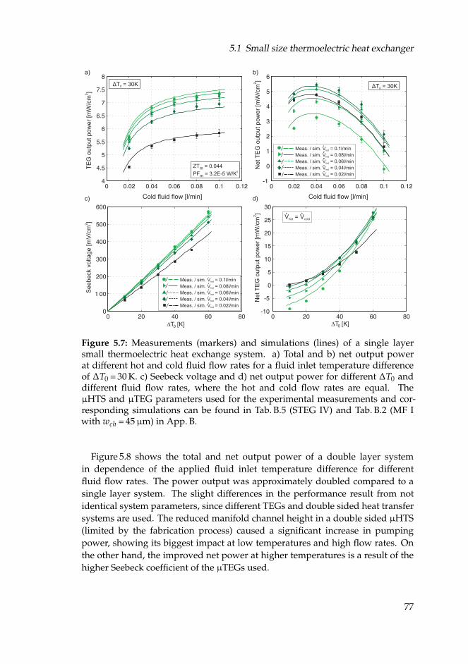
5.1 Small size thermoelectric heat exchanger
a) b)
c) d)
ΔT = 30K0
V = Vhot cold
ZT = 0.044
PF = 3.2E-5 W/Km
m2
ΔT = 30K0
0 0
NetT
EG
outp
ut pow
er
[mW
/cm
]2
NetT
EG
outp
ut pow
er
[mW
/cm
]2
TE
G o
utp
ut pow
er
[mW
/cm
]2
Seebeck v
oltage [m
V/c
m]
2
Meas. / sim. V = 0.1l/min
V = 0.08l/min
Meas. / sim. V = 0.06l/min
Meas. / sim. V = 0.04l/min
Meas. / sim. V = 0.02l/min
hot
hot
hot
hot
hot
Meas. / sim.
Meas. / sim. V = 0.1l/min
V = 0.08l/min
Meas. / sim. V = 0.06l/min
Meas. / sim. V = 0.04l/min
Meas. / sim. V = 0.02l/min
hot
hot
hot
hot
hot
Meas. / sim.
Cold fluid flow [l/min] Cold fluid flow [l/min]
Figure 5.7: Measurements (markers) and simulations (lines) of a single layersmall thermoelectric heat exchange system. a) Total and b) net output powerat different hot and cold fluid flow rates for a fluid inlet temperature differenceof ∆T0 = 30 K. c) Seebeck voltage and d) net output power for different ∆T0 anddifferent fluid flow rates, where the hot and cold flow rates are equal. TheµHTS and µTEG parameters used for the experimental measurements and cor-responding simulations can be found in Tab. B.5 (STEG IV) and Tab. B.2 (MF Iwith wch = 45µm) in App. B.
Figure 5.8 shows the total and net output power of a double layer systemin dependence of the applied fluid inlet temperature difference for differentfluid flow rates. The power output was approximately doubled compared to asingle layer system. The slight differences in the performance result from notidentical system parameters, since different TEGs and double sided heat transfersystems are used. The reduced manifold channel height in a double sided µHTS(limited by the fabrication process) caused a significant increase in pumpingpower, showing its biggest impact at low temperatures and high flow rates. Onthe other hand, the improved net power at higher temperatures is a result of thehigher Seebeck coefficient of the µTEGs used.
77
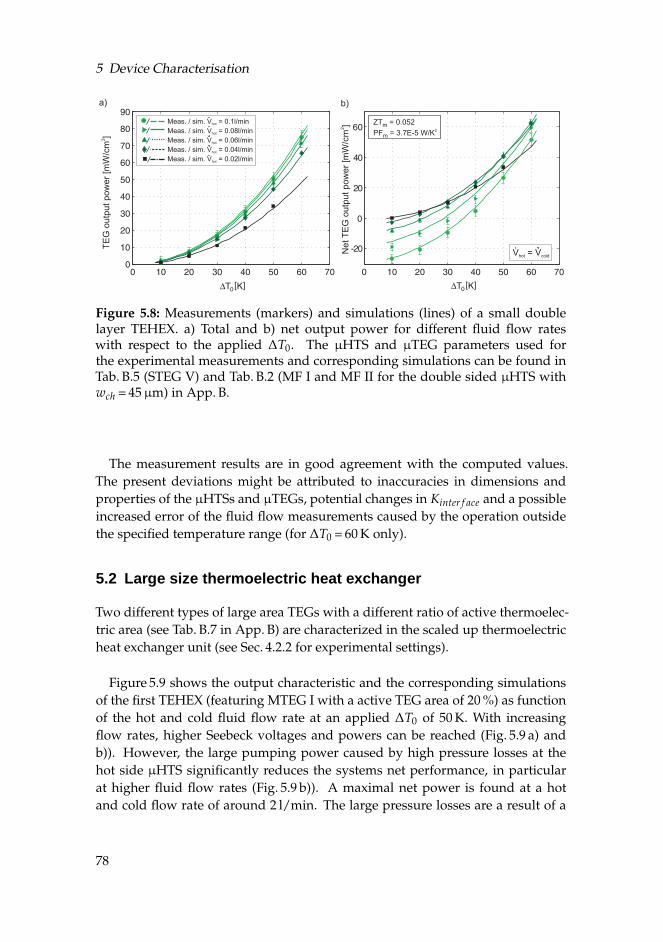
5 Device Characterisation
a) b)
V = Vhot cold
ZT = 0.052
PF = 3.7E-5 W/Km
m2
0
NetT
EG
outp
ut pow
er
[mW
/cm
]2
TE
G o
utp
ut pow
er
[mW
/cm
]2
0
Meas. / sim. V = 0.1l/min
V = 0.08l/min
Meas. / sim. V = 0.06l/min
Meas. / sim. V = 0.04l/min
Meas. / sim. V = 0.02l/min
hot
hot
hot
hot
hot
Meas. / sim.
Figure 5.8: Measurements (markers) and simulations (lines) of a small doublelayer TEHEX. a) Total and b) net output power for different fluid flow rateswith respect to the applied ∆T0. The µHTS and µTEG parameters used forthe experimental measurements and corresponding simulations can be found inTab. B.5 (STEG V) and Tab. B.2 (MF I and MF II for the double sided µHTS withwch = 45µm) in App. B.
The measurement results are in good agreement with the computed values.The present deviations might be attributed to inaccuracies in dimensions andproperties of the µHTSs and µTEGs, potential changes in Kinter f ace and a possibleincreased error of the fluid flow measurements caused by the operation outsidethe specified temperature range (for ∆T0 = 60 K only).
5.2 Large size thermoelectric heat exchanger
Two different types of large area TEGs with a different ratio of active thermoelec-tric area (see Tab. B.7 in App. B) are characterized in the scaled up thermoelectricheat exchanger unit (see Sec. 4.2.2 for experimental settings).
Figure 5.9 shows the output characteristic and the corresponding simulationsof the first TEHEX (featuring MTEG I with a active TEG area of 20 %) as functionof the hot and cold fluid flow rate at an applied ∆T0 of 50 K. With increasingflow rates, higher Seebeck voltages and powers can be reached (Fig. 5.9 a) andb)). However, the large pumping power caused by high pressure losses at thehot side µHTS significantly reduces the systems net performance, in particularat higher fluid flow rates (Fig. 5.9 b)). A maximal net power is found at a hotand cold flow rate of around 2 l/min. The large pressure losses are a result of a
78
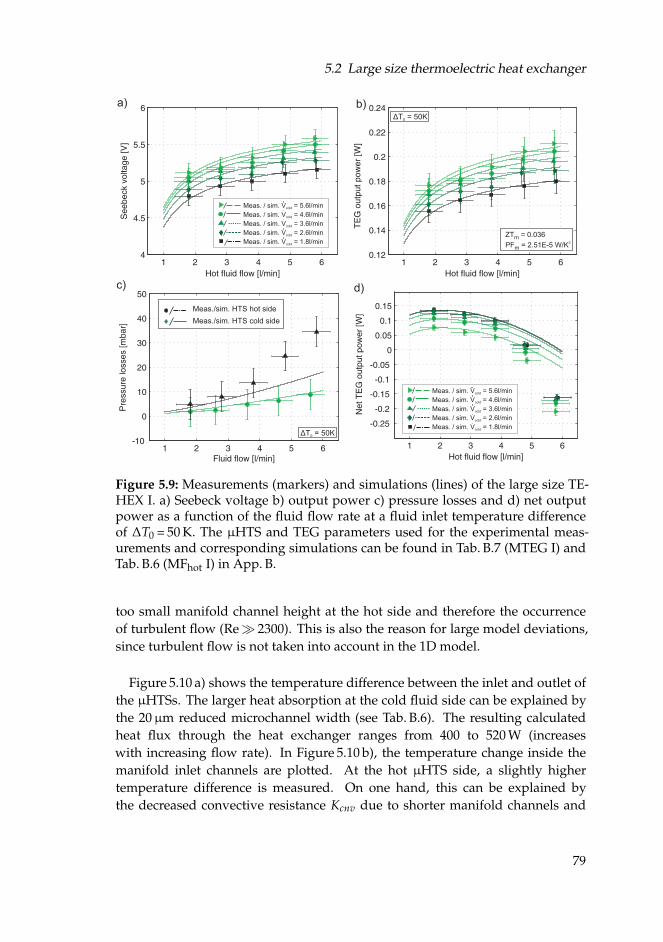
5.2 Large size thermoelectric heat exchanger
a) b)
d)c)
ΔT = 50K0
Meas./sim. HTS hot side
Meas./sim. HTS cold side
Meas. / sim. V = 5.6l/min
V = 4.6l/min
Meas. / sim. V = 3.6l/min
Meas. / sim. V = 2.6l/min
Meas. / sim. V = 1.8l/min
cold
cold
cold
cold
cold
Meas. / sim.
Meas. / sim. V = 5.6l/min
V = 4.6l/min
Meas. / sim. V = 3.6l/min
Meas. / sim. V = 2.6l/min
Meas. / sim. V = 1.8l/min
cold
cold
cold
cold
cold
Meas. / sim.
ZT = 0.036
PF = 2.51E-5 W/Km
m2
ΔT = 50K0
Figure 5.9: Measurements (markers) and simulations (lines) of the large size TE-HEX I. a) Seebeck voltage b) output power c) pressure losses and d) net outputpower as a function of the fluid flow rate at a fluid inlet temperature differenceof ∆T0 = 50 K. The µHTS and TEG parameters used for the experimental meas-urements and corresponding simulations can be found in Tab. B.7 (MTEG I) andTab. B.6 (MFhot I) in App. B.
too small manifold channel height at the hot side and therefore the occurrenceof turbulent flow (Re≫ 2300). This is also the reason for large model deviations,since turbulent flow is not taken into account in the 1D model.
Figure 5.10 a) shows the temperature difference between the inlet and outlet ofthe µHTSs. The larger heat absorption at the cold fluid side can be explained bythe 20µm reduced microchannel width (see Tab. B.6). The resulting calculatedheat flux through the heat exchanger ranges from 400 to 520 W (increaseswith increasing flow rate). In Figure 5.10 b), the temperature change inside themanifold inlet channels are plotted. At the hot µHTS side, a slightly highertemperature difference is measured. On one hand, this can be explained bythe decreased convective resistance Kcnv due to shorter manifold channels and
79
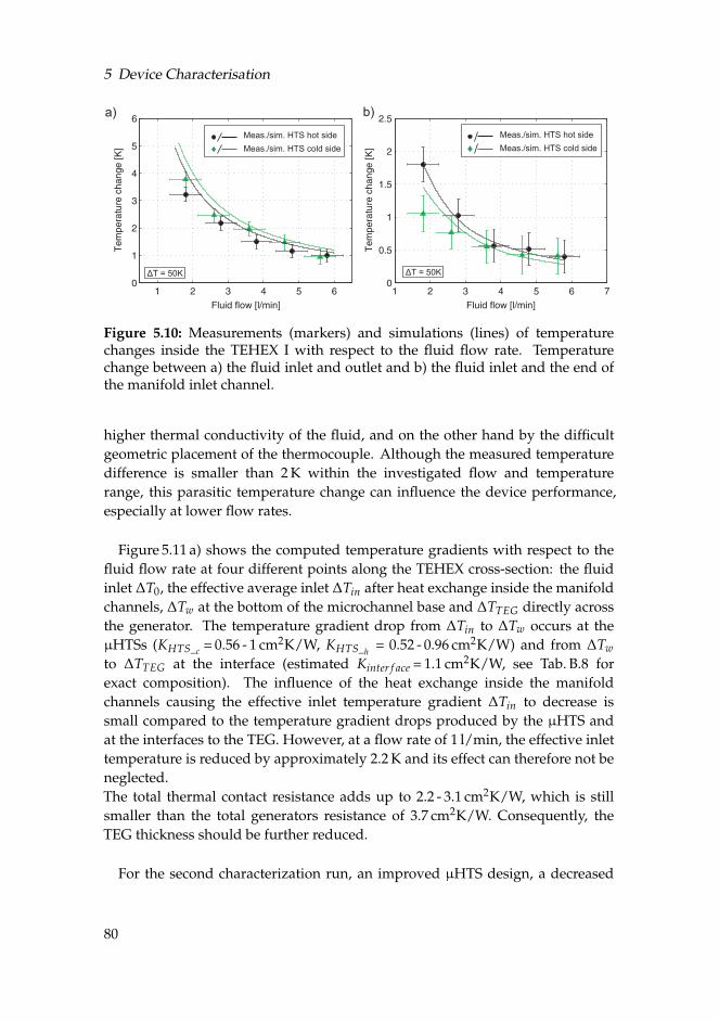
5 Device Characterisation
ΔT = 50K
Meas./sim. HTS hot side
Meas./sim. HTS cold side
a) b)
Meas./sim. HTS hot side
Meas./sim. HTS cold side
ΔT = 50K
Figure 5.10: Measurements (markers) and simulations (lines) of temperaturechanges inside the TEHEX I with respect to the fluid flow rate. Temperaturechange between a) the fluid inlet and outlet and b) the fluid inlet and the end ofthe manifold inlet channel.
higher thermal conductivity of the fluid, and on the other hand by the difficultgeometric placement of the thermocouple. Although the measured temperaturedifference is smaller than 2 K within the investigated flow and temperaturerange, this parasitic temperature change can influence the device performance,especially at lower flow rates.
Figure 5.11 a) shows the computed temperature gradients with respect to thefluid flow rate at four different points along the TEHEX cross-section: the fluidinlet ∆T0, the effective average inlet ∆Tin after heat exchange inside the manifoldchannels, ∆Tw at the bottom of the microchannel base and ∆TTEG directly acrossthe generator. The temperature gradient drop from ∆Tin to ∆Tw occurs at theµHTSs (KHTS_c
= 0.56 - 1 cm2K/W, KHTS_h= 0.52 - 0.96 cm2K/W) and from ∆Tw
to ∆TTEG at the interface (estimated Kinter f ace = 1.1 cm2K/W, see Tab. B.8 forexact composition). The influence of the heat exchange inside the manifoldchannels causing the effective inlet temperature gradient ∆Tin to decrease issmall compared to the temperature gradient drops produced by the µHTS andat the interfaces to the TEG. However, at a flow rate of 1 l/min, the effective inlettemperature is reduced by approximately 2.2 K and its effect can therefore not beneglected.The total thermal contact resistance adds up to 2.2 - 3.1 cm2K/W, which is stillsmaller than the total generators resistance of 3.7 cm2K/W. Consequently, theTEG thickness should be further reduced.
For the second characterization run, an improved µHTS design, a decreased
80
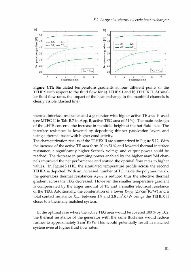
5.2 Large size thermoelectric heat exchanger
a) b)
V = Vhot coldV = Vhot cold
ΔT0
ΔTin
ΔT
ΔTw
TEG
ΔT
ΔT0
in
ΔT
ΔTw
TEG
Te
mp
era
ture
gra
die
nt
[K]
Te
mp
era
ture
gra
die
nt
[K]
Figure 5.11: Simulated temperature gradients at four different points of theTEHEX with respect to the fluid flow for a) TEHEX I and b) TEHEX II. At smal-ler fluid flow rates, the impact of the heat exchange in the manifold channels isclearly visible (dashed line).
thermal interface resistance and a generator with higher active TE area is used(see MTEG II in Tab. B.7 in App. B, active TEG area of 51 %). The main redesignof the µHTS concerns the increase in manifold height at the hot fluid side. Theinterface resistance is lowered by depositing thinner passivation layers andusing a thermal paste with higher conductivity.The characterization results of the TEHEX II are summarized in Figure 5.12. Withthe increase of the active TE area form 20 to 51 % and lowered thermal interfaceresistance, a significantly higher Seebeck voltage and output power could bereached. The decrease in pumping power enabled by the higher manifold chan-nels improved the net performance and shifted the optimal flow rates to highervalues. In Figure 5.11 b), the simulated temperature profile across the secondTEHEX is depicted. With an increased number of TC inside the polymer matrix,the generators thermal resistances KTEG is reduced thus the effective thermalgradient across the TEG decreased. However, the smaller temperature gradientis compensated by the larger amount of TC and a smaller electrical resistanceof the TEG. Additionally, the combination of a lower KTEG (2.7 cm2K/W) and atotal contact resistance Kcon between 1.9 and 2.8 cm2K/W brings the TEHEX IIcloser to a thermally matched system.
In the optimal case where the active TEG area would be covered 100 % by TCs,the thermal resistance of the generator with the same thickness would reducefurther to approximately 2 cm2K/W. This would potentially result in matchedsystem even at higher fluid flow rates.
81
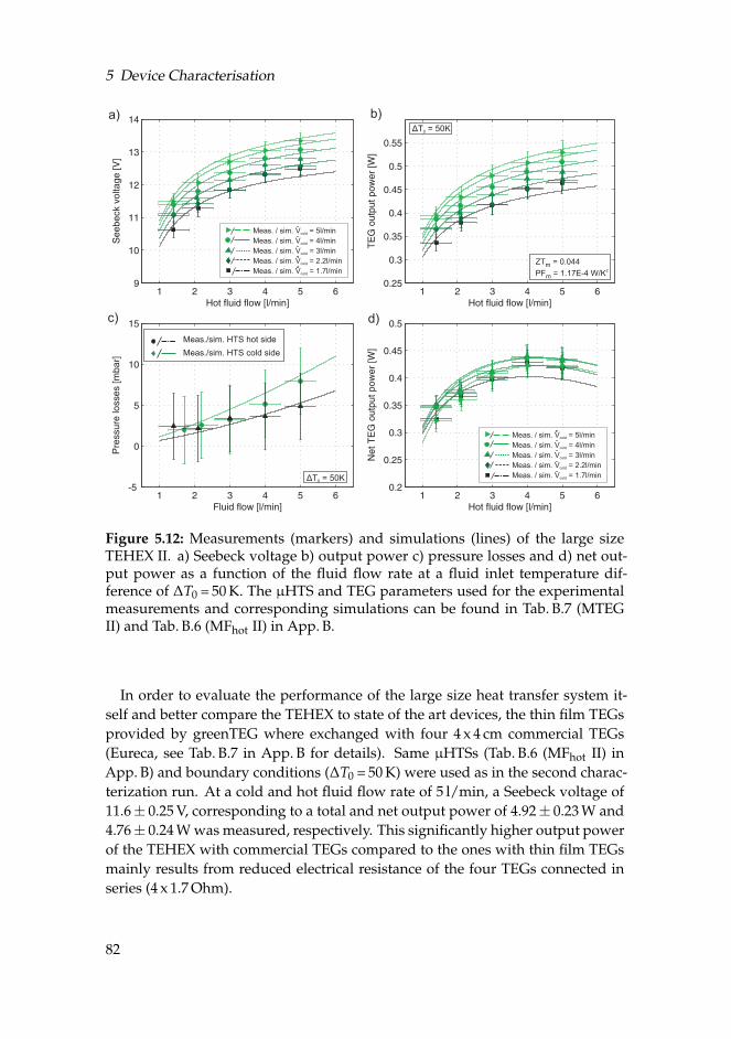
5 Device Characterisation
a) b)
d)c)
Meas./sim. HTS hot side
Meas./sim. HTS cold side
Meas. / sim. V = 5l/min
V = 4l/min
Meas. / sim. V = 3l/min
Meas. / sim. V = 2.2l/min
Meas. / sim. V = 1.7l/min
cold
cold
cold
cold
cold
Meas. / sim.
Meas. / sim. V = 5l/min
V = 4l/min
Meas. / sim. V = 3l/min
Meas. / sim. V = 2.2l/min
Meas. / sim. V = 1.7l/min
cold
cold
cold
cold
cold
Meas. / sim.
ZT = 0.044
PF = 1.17E-4 W/Km
m2
ΔT = 50K0
ΔT = 50K0
Figure 5.12: Measurements (markers) and simulations (lines) of the large sizeTEHEX II. a) Seebeck voltage b) output power c) pressure losses and d) net out-put power as a function of the fluid flow rate at a fluid inlet temperature dif-ference of ∆T0 = 50 K. The µHTS and TEG parameters used for the experimentalmeasurements and corresponding simulations can be found in Tab. B.7 (MTEGII) and Tab. B.6 (MFhot II) in App. B.
In order to evaluate the performance of the large size heat transfer system it-self and better compare the TEHEX to state of the art devices, the thin film TEGsprovided by greenTEG where exchanged with four 4 x 4 cm commercial TEGs(Eureca, see Tab. B.7 in App. B for details). Same µHTSs (Tab. B.6 (MFhot II) inApp. B) and boundary conditions (∆T0 = 50 K) were used as in the second charac-terization run. At a cold and hot fluid flow rate of 5 l/min, a Seebeck voltage of11.6± 0.25 V, corresponding to a total and net output power of 4.92± 0.23 W and4.76± 0.24 W was measured, respectively. This significantly higher output powerof the TEHEX with commercial TEGs compared to the ones with thin film TEGsmainly results from reduced electrical resistance of the four TEGs connected inseries (4 x 1.7 Ohm).
82
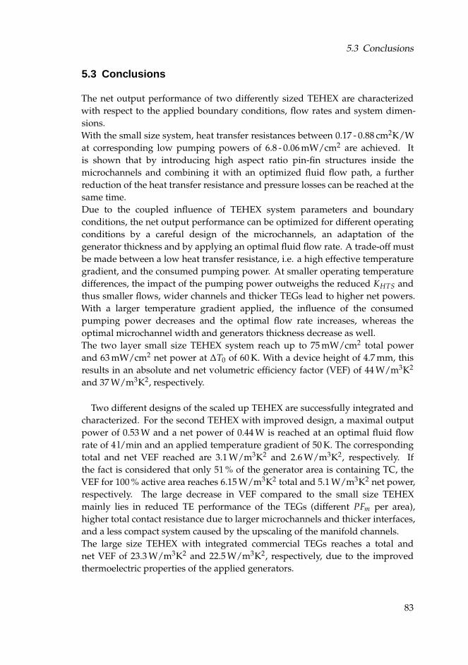
5.3 Conclusions
5.3 Conclusions
The net output performance of two differently sized TEHEX are characterizedwith respect to the applied boundary conditions, flow rates and system dimen-sions.With the small size system, heat transfer resistances between 0.17 - 0.88 cm2K/Wat corresponding low pumping powers of 6.8 - 0.06 mW/cm2 are achieved. Itis shown that by introducing high aspect ratio pin-fin structures inside themicrochannels and combining it with an optimized fluid flow path, a furtherreduction of the heat transfer resistance and pressure losses can be reached at thesame time.Due to the coupled influence of TEHEX system parameters and boundaryconditions, the net output performance can be optimized for different operatingconditions by a careful design of the microchannels, an adaptation of thegenerator thickness and by applying an optimal fluid flow rate. A trade-off mustbe made between a low heat transfer resistance, i.e. a high effective temperaturegradient, and the consumed pumping power. At smaller operating temperaturedifferences, the impact of the pumping power outweighs the reduced KHTS andthus smaller flows, wider channels and thicker TEGs lead to higher net powers.With a larger temperature gradient applied, the influence of the consumedpumping power decreases and the optimal flow rate increases, whereas theoptimal microchannel width and generators thickness decrease as well.The two layer small size TEHEX system reach up to 75 mW/cm2 total powerand 63 mW/cm2 net power at ∆T0 of 60 K. With a device height of 4.7 mm, thisresults in an absolute and net volumetric efficiency factor (VEF) of 44 W/m3K2
and 37 W/m3K2, respectively.
Two different designs of the scaled up TEHEX are successfully integrated andcharacterized. For the second TEHEX with improved design, a maximal outputpower of 0.53 W and a net power of 0.44 W is reached at an optimal fluid flowrate of 4 l/min and an applied temperature gradient of 50 K. The correspondingtotal and net VEF reached are 3.1 W/m3K2 and 2.6 W/m3K2, respectively. Ifthe fact is considered that only 51 % of the generator area is containing TC, theVEF for 100 % active area reaches 6.15 W/m3K2 total and 5.1 W/m3K2 net power,respectively. The large decrease in VEF compared to the small size TEHEXmainly lies in reduced TE performance of the TEGs (different PFm per area),higher total contact resistance due to larger microchannels and thicker interfaces,and a less compact system caused by the upscaling of the manifold channels.The large size TEHEX with integrated commercial TEGs reaches a total andnet VEF of 23.3 W/m3K2 and 22.5 W/m3K2, respectively, due to the improvedthermoelectric properties of the applied generators.
83
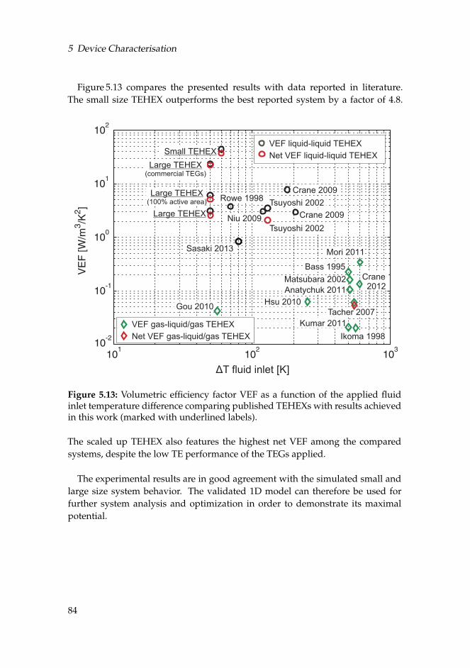
5 Device Characterisation
Figure 5.13 compares the presented results with data reported in literature.The small size TEHEX outperforms the best reported system by a factor of 4.8.
VEF liquid-liquid TEHEX
Net VEF liquid-liquid TEHEX
Rowe 1998
Small TEHEX
Large TEHEX
Large TEHEX(100% active area)
Sasaki 2013
Gou 2010Hsu 2010
Bass 1995
Matsubara 2002
Tacher 2007
Kumar 2011
Ikoma 1998
Mori 2011
Anatychuk 2011
Crane2012
Crane 2009
Tsuyoshi 2002
Niu 2009 Crane 2009
Tsuyoshi 2002
VEF gas-liquid/gas TEHEX
Net VEF gas-liquid/gas TEHEX
Large TEHEX(commercial TEGs)
ΔT fluid inlet [K]
Figure 5.13: Volumetric efficiency factor VEF as a function of the applied fluidinlet temperature difference comparing published TEHEXs with results achievedin this work (marked with underlined labels).
The scaled up TEHEX also features the highest net VEF among the comparedsystems, despite the low TE performance of the TEGs applied.
The experimental results are in good agreement with the simulated small andlarge size system behavior. The validated 1D model can therefore be used forfurther system analysis and optimization in order to demonstrate its maximalpotential.
84
6 Thermoelectric Heat Exchanger Simulations
In this chapter, the validated model described in Chapter 3 is applied for a system-atic analysis and optimization of the characterized thermoelectric heat exchanger.Additionally, a case study is presented, where an estimation of the output per-formance and cost effectiveness for waste heat recovery in a marine propulsionengine is given.
6.1 Simulation results
In the first part of this section, the impact of individual TEG and µHTS paramet-ers on the net output power and net VEF at an applied temperature gradient of50 K are discussed. The second part deals with an overall system optimizationwith respect to the operating conditions.
The following system parameters are used and assumptions are made for thesubsequent simulations:
• Same or similar TEG and µHTS parameters as in the 2nd large size TEHEXare used as standard simulation values (see Tab. B.9 col. 1 in App. B)
• A TEG with 100 % active area is used
• 1 periodic unit of the TEHEX is simulated
• µHTS dimensions are set identical for the hot and cold side (for Sec. 6.1.1only)
• Matched electrical load for maximal power output according to Eq. 3.24
• Pump efficiency and losses at the connecting supply tubes are neglected
6.1.1 Impact of individual parameters
Figure 6.1 shows the influence of the microchannel width, TEG height and See-beck coefficient on the net TEG output power with respect to the fluid flow rate.In Figure 6.2, the impact of most relevant system parameters on the net VEF isshown. In order to visualize the impact of the individual parameters, only the
85
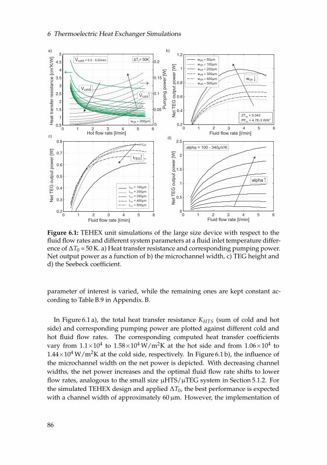
6 Thermoelectric Heat Exchanger Simulations
wch = 50 mμ
wch = 100 mμ
wch = 200 mμ
wch = 300 mμ
wch = 400 mμ
w 5ch = 00 mμ
ΔT = 50K0Vcold = 0.5 - 5.5l/min
Vcold
Vcold
w 200ch = μm
a) b)
l =TEG 100 m
200 m
300 m
400 m
500 m
μ
μ
μ
μ
μ
l =
l =
l =
l =
TEG
TEG
TEG
TEG
c) d)
wch
alpha
alpha = 100 - 340 V/Kμ
lTEG
ZT = 0.045
PF = 4.7E-3 W/Km
m2
Heat tr
ansfe
r re
sis
tance [cm
K/W
]2
NetT
EG
outp
ut pow
er
[W]
Pum
pin
g p
ow
er
[W]
Fluid flow rate [l/min] Fluid flow rate [l/min]
Fluid flow rate [l/min]Hot flow rate [l/min]
NetT
EG
outp
ut pow
er
[W]
NetT
EG
outp
ut pow
er
[W]
Figure 6.1: TEHEX unit simulations of the large size device with respect to thefluid flow rates and different system parameters at a fluid inlet temperature differ-ence of ∆T0 = 50 K. a) Heat transfer resistance and corresponding pumping power.Net output power as a function of b) the microchannel width, c) TEG height andd) the Seebeck coefficient.
parameter of interest is varied, while the remaining ones are kept constant ac-cording to Table B.9 in Appendix. B.
In Figure 6.1 a), the total heat transfer resistance KHTS (sum of cold and hotside) and corresponding pumping power are plotted against different cold andhot fluid flow rates. The corresponding computed heat transfer coefficientsvary from 1.1×10⁴ to 1.58×10⁴ W/m2K at the hot side and from 1.06×10⁴ to1.44×104 W/m2K at the cold side, respectively. In Figure 6.1 b), the influence ofthe microchannel width on the net power is depicted. With decreasing channelwidths, the net power increases and the optimal fluid flow rate shifts to lowerflow rates, analogous to the small size µHTS/µTEG system in Section 5.1.2. Forthe simulated TEHEX design and applied ∆T0, the best performance is expectedwith a channel width of approximately 60µm. However, the implementation of
86
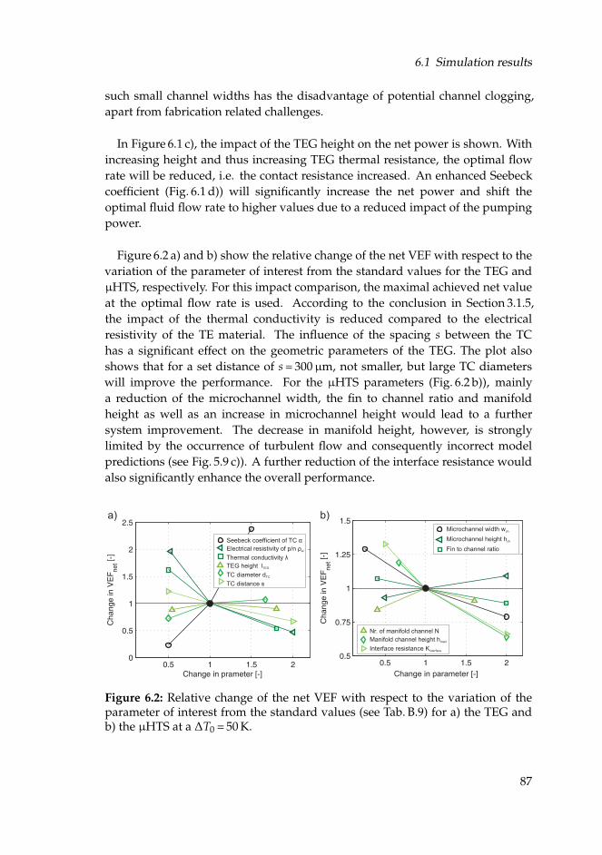
6.1 Simulation results
such small channel widths has the disadvantage of potential channel clogging,apart from fabrication related challenges.
In Figure 6.1 c), the impact of the TEG height on the net power is shown. Withincreasing height and thus increasing TEG thermal resistance, the optimal flowrate will be reduced, i.e. the contact resistance increased. An enhanced Seebeckcoefficient (Fig. 6.1 d)) will significantly increase the net power and shift theoptimal fluid flow rate to higher values due to a reduced impact of the pumpingpower.
Figure 6.2 a) and b) show the relative change of the net VEF with respect to thevariation of the parameter of interest from the standard values for the TEG andµHTS, respectively. For this impact comparison, the maximal achieved net valueat the optimal flow rate is used. According to the conclusion in Section 3.1.5,the impact of the thermal conductivity is reduced compared to the electricalresistivity of the TE material. The influence of the spacing s between the TChas a significant effect on the geometric parameters of the TEG. The plot alsoshows that for a set distance of s = 300µm, not smaller, but large TC diameterswill improve the performance. For the µHTS parameters (Fig. 6.2 b)), mainlya reduction of the microchannel width, the fin to channel ratio and manifoldheight as well as an increase in microchannel height would lead to a furthersystem improvement. The decrease in manifold height, however, is stronglylimited by the occurrence of turbulent flow and consequently incorrect modelpredictions (see Fig. 5.9 c)). A further reduction of the interface resistance wouldalso significantly enhance the overall performance.
Microchannel width w
icrochannel height h
ch
chM
Fin to channel ratio
Nr. of manifold channel N
Manifold channel height h
Interface resistance K
mani
interface
b)
Change in parameter [-]
Seebeck coefficient of TC
ctrical resistivity of p/n
TEG height l
TC diameter d
TC distance s
α
ρel
TEG
TC
Ele
Thermal conductivity λ
a)
Figure 6.2: Relative change of the net VEF with respect to the variation of theparameter of interest from the standard values (see Tab. B.9) for a) the TEG andb) the µHTS at a ∆T0 = 50 K.
87
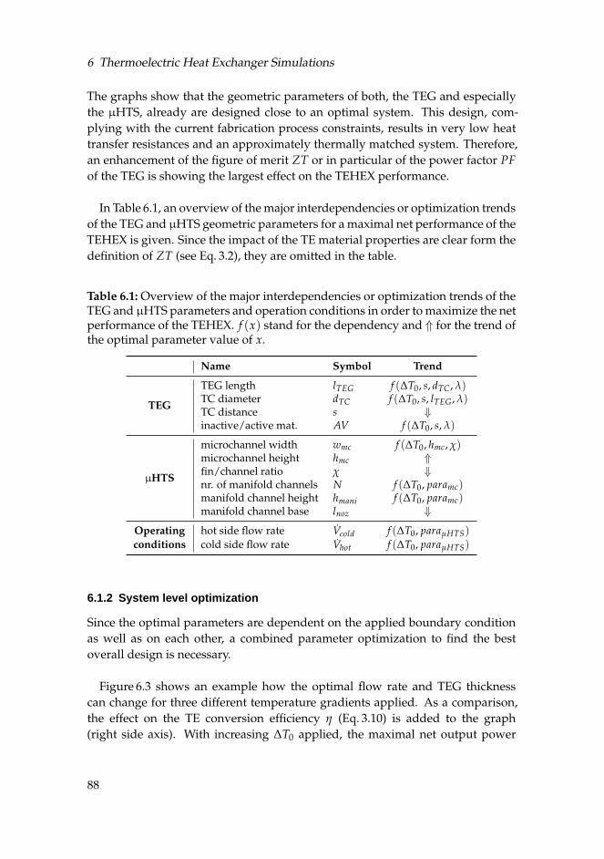
6 Thermoelectric Heat Exchanger Simulations
The graphs show that the geometric parameters of both, the TEG and especiallythe µHTS, already are designed close to an optimal system. This design, com-plying with the current fabrication process constraints, results in very low heattransfer resistances and an approximately thermally matched system. Therefore,an enhancement of the figure of merit ZT or in particular of the power factor PF
of the TEG is showing the largest effect on the TEHEX performance.
In Table 6.1, an overview of the major interdependencies or optimization trendsof the TEG and µHTS geometric parameters for a maximal net performance of theTEHEX is given. Since the impact of the TE material properties are clear form thedefinition of ZT (see Eq. 3.2), they are omitted in the table.
Table 6.1: Overview of the major interdependencies or optimization trends of theTEG and µHTS parameters and operation conditions in order to maximize the netperformance of the TEHEX. f (x) stand for the dependency and ⇑ for the trend ofthe optimal parameter value of x.
Name Symbol Trend
TEG
TEG length lTEG f (∆T0, s, dTC, λ)TC diameter dTC f (∆T0, s, lTEG, λ)TC distance s ⇓inactive/active mat. AV f (∆T0, s, λ)
µHTS
microchannel width wmc f (∆T0, hmc, χ)microchannel height hmc ⇑fin/channel ratio χ ⇓nr. of manifold channels N f (∆T0, paramc)manifold channel height hmani f (∆T0, paramc)manifold channel base lnoz ⇓
Operating hot side flow rate Vcold f (∆T0, paraµHTS)conditions cold side flow rate Vhot f (∆T0, paraµHTS)
6.1.2 System level optimization
Since the optimal parameters are dependent on the applied boundary conditionas well as on each other, a combined parameter optimization to find the bestoverall design is necessary.
Figure 6.3 shows an example how the optimal flow rate and TEG thicknesscan change for three different temperature gradients applied. As a comparison,the effect on the TE conversion efficiency η (Eq. 3.10) is added to the graph(right side axis). With increasing ∆T0 applied, the maximal net output power
88
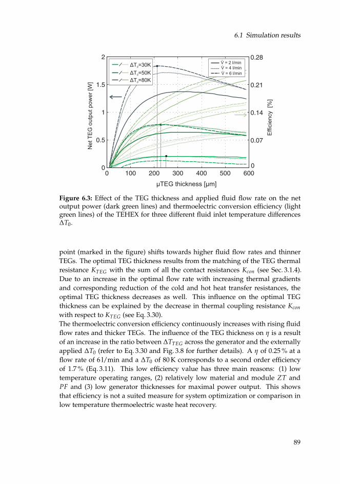
6.1 Simulation results
µTEG thickness [µm]
ΔT =30K0
ΔT =50K0
ΔT =80K0
Effic
ien
cy
[%]
V = 2 l/min
V = 4 l/min
V = 6 l/min
Ne
tT
EG
ou
tpu
t p
ow
er
[W]
Figure 6.3: Effect of the TEG thickness and applied fluid flow rate on the netoutput power (dark green lines) and thermoelectric conversion efficiency (lightgreen lines) of the TEHEX for three different fluid inlet temperature differences∆T0.
point (marked in the figure) shifts towards higher fluid flow rates and thinnerTEGs. The optimal TEG thickness results from the matching of the TEG thermalresistance KTEG with the sum of all the contact resistances Kcon (see Sec. 3.1.4).Due to an increase in the optimal flow rate with increasing thermal gradientsand corresponding reduction of the cold and hot heat transfer resistances, theoptimal TEG thickness decreases as well. This influence on the optimal TEGthickness can be explained by the decrease in thermal coupling resistance Kcon
with respect to KTEG (see Eq. 3.30).The thermoelectric conversion efficiency continuously increases with rising fluidflow rates and thicker TEGs. The influence of the TEG thickness on η is a resultof an increase in the ratio between ∆TTEG across the generator and the externallyapplied ∆T0 (refer to Eq. 3.30 and Fig. 3.8 for further details). A η of 0.25 % at aflow rate of 6 l/min and a ∆T0 of 80 K corresponds to a second order efficiencyof 1.7 % (Eq. 3.11). This low efficiency value has three main reasons: (1) lowtemperature operating ranges, (2) relatively low material and module ZT andPF and (3) low generator thicknesses for maximal power output. This showsthat efficiency is not a suited measure for system optimization or comparison inlow temperature thermoelectric waste heat recovery.
89
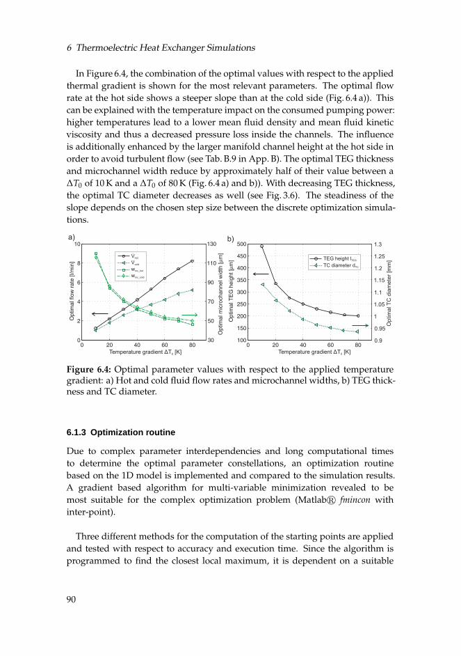
6 Thermoelectric Heat Exchanger Simulations
In Figure 6.4, the combination of the optimal values with respect to the appliedthermal gradient is shown for the most relevant parameters. The optimal flowrate at the hot side shows a steeper slope than at the cold side (Fig. 6.4 a)). Thiscan be explained with the temperature impact on the consumed pumping power:higher temperatures lead to a lower mean fluid density and mean fluid kineticviscosity and thus a decreased pressure loss inside the channels. The influenceis additionally enhanced by the larger manifold channel height at the hot side inorder to avoid turbulent flow (see Tab. B.9 in App. B). The optimal TEG thicknessand microchannel width reduce by approximately half of their value between a∆T0 of 10 K and a ∆T0 of 80 K (Fig. 6.4 a) and b)). With decreasing TEG thickness,the optimal TC diameter decreases as well (see Fig. 3.6). The steadiness of theslope depends on the chosen step size between the discrete optimization simula-tions.
b)a)
Vhot
V
w
w
cold
mc_hot
mc_cold
0.9
0.95
1
1.05
1.1
1.15
1.2
1.25
1.3
Optim
alT
C d
iam
ete
r [m
m]TEG height
TC diameter dTC
lTEG
Temperature gradient T [K]Δ 0Temperature gradient T [K]Δ 0
Figure 6.4: Optimal parameter values with respect to the applied temperaturegradient: a) Hot and cold fluid flow rates and microchannel widths, b) TEG thick-ness and TC diameter.
6.1.3 Optimization routine
Due to complex parameter interdependencies and long computational timesto determine the optimal parameter constellations, an optimization routinebased on the 1D model is implemented and compared to the simulation results.A gradient based algorithm for multi-variable minimization revealed to bemost suitable for the complex optimization problem (Matlabr fmincon withinter-point).
Three different methods for the computation of the starting points are appliedand tested with respect to accuracy and execution time. Since the algorithm isprogrammed to find the closest local maximum, it is dependent on a suitable
90
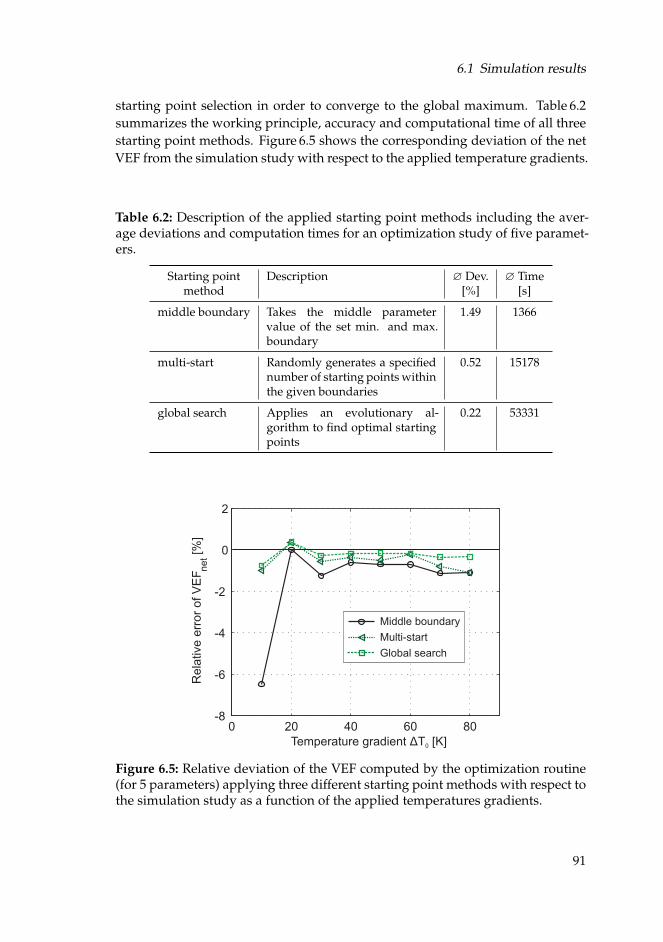
6.1 Simulation results
starting point selection in order to converge to the global maximum. Table 6.2summarizes the working principle, accuracy and computational time of all threestarting point methods. Figure 6.5 shows the corresponding deviation of the netVEF from the simulation study with respect to the applied temperature gradients.
Table 6.2: Description of the applied starting point methods including the aver-age deviations and computation times for an optimization study of five paramet-ers.
Starting point Description ∅ Dev. ∅ Timemethod [%] [s]
middle boundary Takes the middle parametervalue of the set min. and max.boundary
1.49 1366
multi-start Randomly generates a specifiednumber of starting points withinthe given boundaries
0.52 15178
global search Applies an evolutionary al-gorithm to find optimal startingpoints
0.22 53331
0 20 40 60 80-8
-6
-4
-2
0
2
Temperature gradient T [K]Δ 0
Rela
tive e
rror
of V
EF
net[%
]
Middle boundary
Global search
Multi-start
Figure 6.5: Relative deviation of the VEF computed by the optimization routine(for 5 parameters) applying three different starting point methods with respect tothe simulation study as a function of the applied temperatures gradients.
91
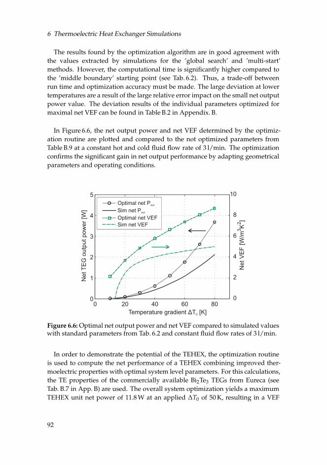
6 Thermoelectric Heat Exchanger Simulations
The results found by the optimization algorithm are in good agreement withthe values extracted by simulations for the ’global search’ and ’multi-start’methods. However, the computational time is significantly higher compared tothe ’middle boundary’ starting point (see Tab. 6.2). Thus, a trade-off betweenrun time and optimization accuracy must be made. The large deviation at lowertemperatures are a result of the large relative error impact on the small net outputpower value. The deviation results of the individual parameters optimized formaximal net VEF can be found in Table B.2 in Appendix. B.
In Figure 6.6, the net output power and net VEF determined by the optimiz-ation routine are plotted and compared to the not optimized parameters fromTable B.9 at a constant hot and cold fluid flow rate of 3 l/min. The optimizationconfirms the significant gain in net output performance by adapting geometricalparameters and operating conditions.
20 40 60 800
2
4
6
8
10
Ne
t V
EF
[W
/m3K
2]
00
1
2
3
4
5
NetT
EG
outp
ut pow
er
[W]
Temperature gradient T [K]Δ 0
Optimal net Pout
Sim net P
Optimal net VEF
Sim net VEF
out
Figure 6.6: Optimal net output power and net VEF compared to simulated valueswith standard parameters from Tab. 6.2 and constant fluid flow rates of 3 l/min.
In order to demonstrate the potential of the TEHEX, the optimization routineis used to compute the net performance of a TEHEX combining improved ther-moelectric properties with optimal system level parameters. For this calculations,the TE properties of the commercially available Bi2Te3 TEGs from Eureca (seeTab. B.7 in App. B) are used. The overall system optimization yields a maximumTEHEX unit net power of 11.8 W at an applied ∆T0 of 50 K, resulting in a VEF
92
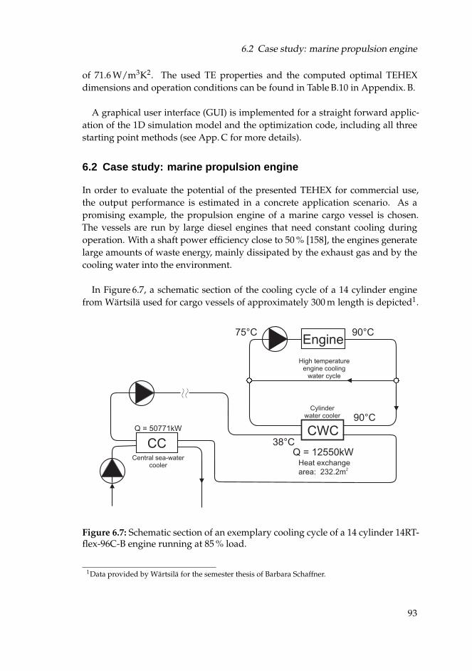
6.2 Case study: marine propulsion engine
of 71.6 W/m3K2. The used TE properties and the computed optimal TEHEXdimensions and operation conditions can be found in Table B.10 in Appendix. B.
A graphical user interface (GUI) is implemented for a straight forward applic-ation of the 1D simulation model and the optimization code, including all threestarting point methods (see App. C for more details).
6.2 Case study: marine propulsion engine
In order to evaluate the potential of the presented TEHEX for commercial use,the output performance is estimated in a concrete application scenario. As apromising example, the propulsion engine of a marine cargo vessel is chosen.The vessels are run by large diesel engines that need constant cooling duringoperation. With a shaft power efficiency close to 50 % [158], the engines generatelarge amounts of waste energy, mainly dissipated by the exhaust gas and by thecooling water into the environment.
In Figure 6.7, a schematic section of the cooling cycle of a 14 cylinder enginefrom Wärtsilä used for cargo vessels of approximately 300 m length is depicted1.
CC
Engine
Central sea-watercooler
CWC
Cylinderwater cooler
High temperatureengine cooling
water cycle
75°C 90°C
90°C
Q = 12550kW38°C
Heat exchange
area: 232.2m2
Q = 50771kW
Figure 6.7: Schematic section of an exemplary cooling cycle of a 14 cylinder 14RT-flex-96C-B engine running at 85 % load.
1Data provided by Wärtsilä for the semester thesis of Barbara Schaffner.
93
6 Thermoelectric Heat Exchanger Simulations
The given data of the sample cooling cycle with a separate high temperaturecycle for the engine correspond to normal propulsion under 85 % load. At thecylinder water cooler (CWC) heat exchanger, a water inlet temperature gradientof 52 K is available and a total heat amount of 12550 kW needs to be dissipated.The heat extracted by the engine jacket water corresponds to approx. 6.3 % ofthe total fuel input [158]. There are two possibilities to recover a part of thiswaste heat: either with an installed pre-cooler TEHEX or by directly replacingthe existing heat exchanger with the proposed TEHEX. The latter option will bediscussed here in more detail.
With the optimized design under optimal fluid flow rates for maximal netpower and at the ∆T0 of 52 K, a total heat flux of 873 W can be dissipated byone TEHEX unit. In order to extract the total necessary heat of 12550 kW, atotal heat exchange area of 92 m2 is needed. This is a factor 2.5 smaller thanthe area of the actually implemented CWC heat exchanger. The additionalthermal resistance introduced by the thin film TEG can thus be successfullycompensated with the efficient heat transfer system resulting in a higher heatflux per heat exchange area. With the current TE material properties of themodules (PFm = 4.7×10⁻² W/K2, ZTm = 0.045), a total of 16.8 kW net powercould be generated.In Figure 6.8, the net power of the directly installed TEHEX is plotted withrespect to the power factor PFm and TE figure of merit ZTm. The three markedpoints in the graph correspond to the generator’s TE properties with (1) thecurrently used Bi2Te3 material (material 1), (2) the state of the art single crystalBi2Te3 [159] (material 2) and (3) nanostructured material with enhanced powerfactor like reported for Bi0.52Sb1.48Te3 p-type material in [160] (material 3). Withan improved material, up to 145 kW could potentially be recovered with theTEHEX installed in the high temperature engine cooling cycle and used to coverparts of the required ship service power.
This is only one possible example of waste heat recovery from the marine en-gine. Several other waste heat sources are available within the entire propulsionsand service power plant, such as the central sea water cooler, the lubricant oil sys-tem, scavenge air cooler and the exhaust gas of the main and auxiliary engines[158].
6.2.1 Cost analysis
Based on the net output power values presented in the last section, the cost ef-fectiveness of the TEHEX for the application in marine propulsion engines is es-timated. In Figure 6.9 a), the investment cost per generated Watt is plotted with
94
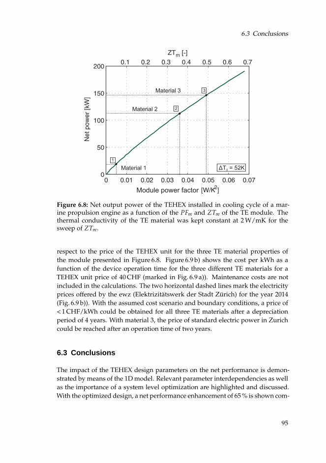
6.3 Conclusions
ZT [-]m
Material 1
Material 3
Material 2 2
1
3
ΔT = 52K0
Module power factor
Figure 6.8: Net output power of the TEHEX installed in cooling cycle of a mar-ine propulsion engine as a function of the PFm and ZTm of the TE module. Thethermal conductivity of the TE material was kept constant at 2 W/mK for thesweep of ZTm.
respect to the price of the TEHEX unit for the three TE material properties ofthe module presented in Figure 6.8. Figure 6.9 b) shows the cost per kWh as afunction of the device operation time for the three different TE materials for aTEHEX unit price of 40 CHF (marked in Fig. 6.9 a)). Maintenance costs are notincluded in the calculations. The two horizontal dashed lines mark the electricityprices offered by the ewz (Elektrizitätswerk der Stadt Zürich) for the year 2014(Fig. 6.9 b)). With the assumed cost scenario and boundary conditions, a price of< 1 CHF/kWh could be obtained for all three TE materials after a depreciationperiod of 4 years. With material 3, the price of standard electric power in Zurichcould be reached after an operation time of two years.
6.3 Conclusions
The impact of the TEHEX design parameters on the net performance is demon-strated by means of the 1D model. Relevant parameter interdependencies as wellas the importance of a system level optimization are highlighted and discussed.With the optimized design, a net performance enhancement of 65 % is shown com-
95
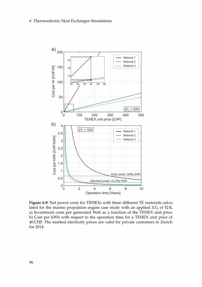
6 Thermoelectric Heat Exchanger Simulations
0 100 200 300 400 5000
50
100
150
200
TEHEX unit price [CHF]
Cost per
W [C
HF
/W]
a)
Material 1
Material 3
Material 2
ΔT = 52K0
10 20 30 40 50 60
10
20
30
0 2 4 6 8 100
0.5
1
1.5
2
2.5
3
3.5
4
Operation time [Years]
Cost per
kW
h [C
HF
/kW
h]
ΔT = 52K0
Solar power: 65Rp./kWh
Standard power: 22.2Rp./kWh
b)
Material 1
Material 3
Material 2
Figure 6.9: Net power costs for TEHEXs with three different TE materials calcu-lated for the marine propulsion engine case study with an applied ∆T0 of 52 K.a) Investment costs per generated Watt as a function of the TEHEX unit price.b) Cost per kWh with respect to the operation time for a TEHEX unit price of40 CHF. The marked electricity prices are valid for private customers in Zurichfor 2014.
96
6.3 Conclusions
pared to a TEHEX with the initial dimensions and a fixed fluid rate of 3l/min ata ∆T0 of 50 K. To demonstrate the potential of the TEHEX, the system level optim-ization is used to compute the net performance of a device featuring improvedthermoelectric properties. With a ZTm and PFm of 0.5 and 7.52×10⁻² W/K2, re-spectively, a net VEF of 71.6 W/m3K2 could potentially be achieved, which is anorder of magnitude higher than best reported values.An optimization routine is implemented and verified, which allows for a straight-forward and fast system optimization for given specific boundary conditions andTE parameters of the module. With the optimized TEHEX design, a realistic casestudy on the application in a marine propulsion engine is conducted. It is shownthat by installing the TEHEX in the engine cylinder cooling cycle, up to 145 kWcould be harvested by applying improved TE materials. This power output cor-responds to 1.16 % net and 10.1 % 2nd order efficiency, which is considerable for ahigh heat flux application and the low temperature of the waste heat recovered.A cost analysis yielded a minimal investment cost of 4 CHF/Watt or a power costof 0.11 CHF/kWh for the assumed cost scenario and a payback period of 4 years.Furthermore, it is concluded that not the efficiency but rather the total net powermust taken as a measure to compare different TEHEX systems for low temperat-ure waste heat recovery in high heat flux applications.
97

7 Conclusion and Outlook
To overcome the present limitations of thermoelectric heat exchangers for lowtemperature waste heat recovery, a novel concept combining multi-layer highperformance heat transfer systems and thin film generators is introduced. TheµHTS consists of polymer manifold distribution channels sandwiched betweencopper plates featuring high aspect ratio microchannels. The system combinesthe advantage of very efficient heat dissipation and supply enabled by themicrochannels as well as low pressure losses and homogeneous heat transferenabled by the manifold distribution channels. Both characteristics are essentialfor an enhanced net performance of the TEHEX. Additionally, the implementa-tion of an efficient µHTS allows for the application of µTEGs with thicknessesin the micrometer range in order to achieve a thermally matched system andthus optimal system conditions. This brings several advantages with respect tocompactness, weight and cost and makes the system suitable for high heat fluxwaste heat recovery applications.
The proposed system is fabricated on two different size scales: a small8 x 8 mm system for concept validation, detailed device analysis and potentialdemonstration and a large 9 x 9 cm system to prove the feasibility of a scalablefabrication process and investigate the suitability of the system for a commercialapplication in WHR. The main focus of the technology development is set on thefabrication of high aspect ratio copper microchannels. The small size fabricationprocess is based on electrochemical deposition of copper into a SU-8 moldstructured by photolithography. Microchannel widths down to 30µm with achannel aspect ratio of 7 are reached. The fabrication of additional heat transferenhancement structures inside the microchannels resulted in vertical 30µm widepin-fins with aspect ratios of up to 8.1. An epoxy based bonding process isdeveloped to assemble the microchannel chips to the polymer manifold channelsfabricated by means of microstereolithography.For the large size system, two microchannel fabrication approaches are evaluated:a bottom-up approach based on electroplating into a dry film resist mold and atop-down approach based on photolithography and etching. The latter approachyielded superior results with respect to process simplicity, processing timeand fin to channel ratios and was therefore applied for the final demonstratorfabrication. Microchannel plates with 170± 10µm high and 220± 15µm widechannels and a fin to channel ratio of 0.5± 0.1 are implemented in the large sizeTEHEX.
99
7 Conclusion and Outlook
The fabricated and assembled TEHEX are characterized in controlled fluidloops with respect to the generated net output power and net volumetricefficiency factor. The small size µHTS achieved heat transfer resistancesbetween 0.17 and 0.88 cm2K/W at corresponding low pumping powers of6.8 - 0.06 mW/cm2. By combining pin-fin structures with rounded inlet/outletnozzles, a further overall µHTS improvement can be reached. Due to thecoupled influence of the µHTS and µTEG parameters and boundary conditions,the system’s net output performance can be optimized for different operatingconditions by the applied fluid flow rate and optimal system dimensions. With atwo unit TEHEX, a net power of 63 mW/cm2 at ∆T0 of 60 K is reached, resultingin a net VEF of 37 W/m3K2. This value can be further enhanced by reducingthe µTEG thickness for optimal thermal matching and by implementing theproposed µHTS heat transfer improvements into the TEHEX.Furthermore, it is concluded that for systems with good thermal coupling, thethermoelectric material optimization must focus more on the power factor in-stead of the figure of merit ZT itself, since the influence of the thermal resistanceof the TE material is reduced.The improved scaled up TEHEX with a 51 % active TEG area reached a maximalnet power of 0.44 W at an optimal fluid flow rate of 4 l/min and an appliedtemperature gradient of 50 K. With the total volume of only 67.7 cm3, a netVEF of 2.6 W/m3K2 is achieved for the current TEG and 5.1 W/m3K2 could bereached for a 100 % active area TEG (see Fig. 5.13 in Chap. 5.3). Despite the lowTE efficiency of the applied generators, this is the highest reported net VEF value,demonstrating the potential of the compact system over state of the art TEHEX.
A one-dimensional numerical TEHEX model is developed based on a networkof thermal resistances. The model combines a precise TEG model including Jouleheating and Peltier effect with a µHTS model implemented in an iterative compu-tation routine. The influence of the temperature-dependent fluid parameters onthe thermal resistance and pressure loss calculations in the µHTS is accounted forby introducing a discrete temperature profile inside the microchannels. Due tothe small heat exchange between the manifold and the microchannel, a gradualfluid temperature change along the manifold channels is modelled as well. Theimplemented model allows for analysis and optimization of most geometric andmaterial properties of the TEHEX, and shows a good agreement with the experi-mental results.The verified model is applied for a detailed investigation of parameter impactsand interdependencies as well as a system level optimization. The impact of thepumping power on the overall system performance is large at smaller operating
100
temperature differences. Thus, smaller flow rates and wider channels and there-fore thicker µTEGs and larger TC diameters lead to higher net performances inthis operation regime. With a larger temperature gradient applied, the influenceof the consumed pumping power decreases and the optimal flow rate increases,whereas the optimal microchannel width, µTEG thickness and TC diameter de-crease. With a system level optimized TEHEX, a significant net performance en-hancement and a net power gain starting form an applied thermal gradient of10 K is predicted.Based on the findings of the optimization study, a concrete example of wasteheat recovery from a marine propulsion engine is calculated. With improved TEmaterials up to 145 kW could be harvested from the high temperature cylindercooling cycle at an estimated investment cost of 4 CHF/Watt for a TEHEX unitcost of 40 CHF (footprint area of 81 cm2).
Outlook
With respect to a further improvement of the technology, several investigationsneed to be conducted.A reliable protective microchannel coating against corrosion and potentialresidue deposition must be developed and applied. The lifetime expectation andreliability of the TEHEX should be tested in an application related environment,in particular with respect to the durability of the polymer manifold channels.The effects of potential microchannel clogging caused by impurities in the feedwater should be investigated in order to figure out the minimal applicablemicrochannel width for the specific applications or tolerable pressure lossintroduced by fluid filters. An increase in microchannel height based on thebottom-up approach or alternative fabrication technologies should be explored.Moreover, further device upscaling will be necessary for most waste heatrecovery applications.
As a next step, a promising application should be selected for field experiments,e.g. the proposed marine propulsion engine. The implemented design optimiz-ation tool can be applied to compute the optimal TEHEX design within givenfabrication technology constraints and microchannel size limits imposed by theapplication. Finally, first prototypes can be built, installed and tested in a fieldenvironment.Nevertheless, high density TEGs, improved TE material properties as well as lowfabrication cost of the TEHEX are essential for successful commercialization.
101

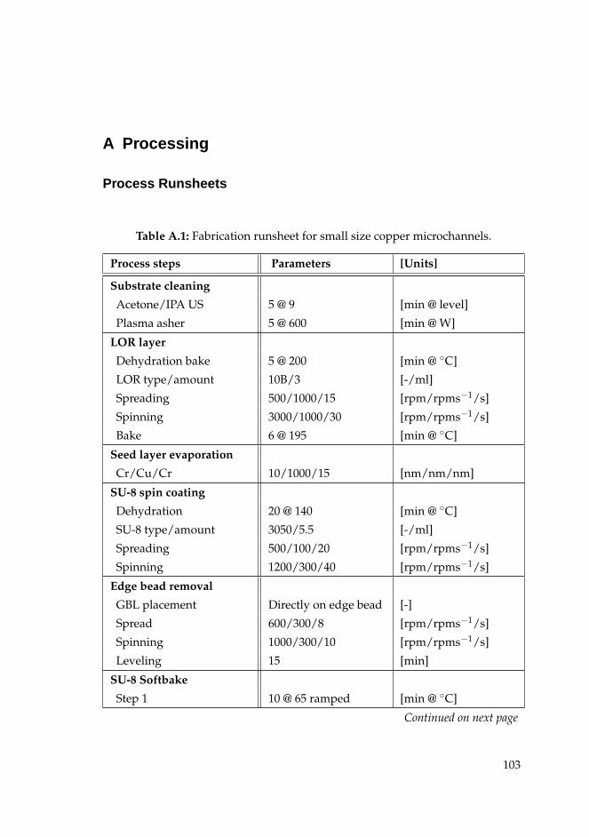
A Processing
Process Runsheets
Table A.1: Fabrication runsheet for small size copper microchannels.
Process steps Parameters [Units]
Substrate cleaning
Acetone/IPA US 5 @ 9 [min @ level]
Plasma asher 5 @ 600 [min @ W]
LOR layer
Dehydration bake 5 @ 200 [min @ C]
LOR type/amount 10B/3 [-/ml]
Spreading 500/1000/15 [rpm/rpms−1/s]
Spinning 3000/1000/30 [rpm/rpms−1/s]
Bake 6 @ 195 [min @ C]
Seed layer evaporation
Cr/Cu/Cr 10/1000/15 [nm/nm/nm]
SU-8 spin coating
Dehydration 20 @ 140 [min @ C]
SU-8 type/amount 3050/5.5 [-/ml]
Spreading 500/100/20 [rpm/rpms−1/s]
Spinning 1200/300/40 [rpm/rpms−1/s]
Edge bead removal
GBL placement Directly on edge bead [-]
Spread 600/300/8 [rpm/rpms−1/s]
Spinning 1000/300/10 [rpm/rpms−1/s]
Leveling 15 [min]
SU-8 Softbake
Step 1 10 @ 65 ramped [min @ C]
Continued on next page
103
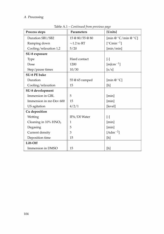
A Processing
Table A.1 – Continued from previous page
Process steps Parameters [Units]
Duration SB1/SB2 15 @ 80/55 @ 80 [min @ C/min @ C]
Ramping down ∼1.2 to RT [Cmin−1]
Cooling/relaxation 1,2 5/20 [min/min]
SU-8 exposure
Type Hard contact [-]
Dose 1200 [mJcm−1]
Step/pause times 10/30 [s/s]
SU-8 PE bake
Duration 55 @ 65 ramped [min @ C]
Cooling/relaxation 15 [h]
SU-8 development
Immersion in GBL 5 [min]
Immersion in mr-Dev 600 15 [min]
US agitation 4/2/1 [level]
Cu deposition
Wetting IPA/DI Water [-]
Cleaning in 10% HNO3 1 [min]
Degasing 5 [min]
Current density 3 [Adm−2]
Deposition time 15 [h]
Lift-Off
Immersion in DMSO 15 [h]
104
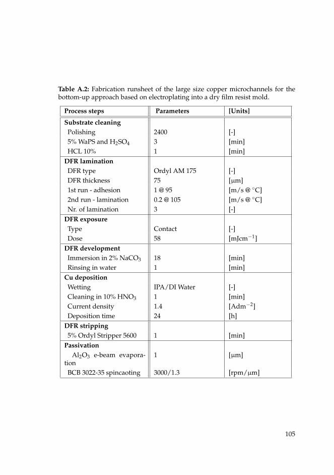
Table A.2: Fabrication runsheet of the large size copper microchannels for thebottom-up approach based on electroplating into a dry film resist mold.
Process steps Parameters [Units]
Substrate cleaning
Polishing 2400 [-]
5% WaPS and H2SO4 3 [min]
HCL 10% 1 [min]
DFR lamination
DFR type Ordyl AM 175 [-]
DFR thickness 75 [µm]
1st run - adhesion 1 @ 95 [m/s @ C]
2nd run - lamination 0.2 @ 105 [m/s @ C]
Nr. of lamination 3 [-]
DFR exposure
Type Contact [-]
Dose 58 [mJcm−1]
DFR development
Immersion in 2% NaCO3 18 [min]
Rinsing in water 1 [min]
Cu deposition
Wetting IPA/DI Water [-]
Cleaning in 10% HNO3 1 [min]
Current density 1.4 [Adm−2]
Deposition time 24 [h]
DFR stripping
5% Ordyl Stripper 5600 1 [min]
Passivation
Al2O3 e-beam evapora-tion
1 [µm]
BCB 3022-35 spincaoting 3000/1.3 [rpm/µm]
105
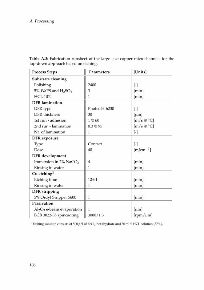
A Processing
Table A.3: Fabrication runsheet of the large size copper microchannels for thetop-down approach based on etching.
Process Steps Parameters [Units]
Substrate cleaning
Polishing 2400 [-]
5% WaPS and H2SO4 3 [min]
HCL 10% 1 [min]
DFR lamination
DFR type Photec H-6230 [-]
DFR thickness 30 [µm]
1st run - adhesion 1 @ 60 [m/s @ C]
2nd run - lamination 0.3 @ 95 [m/s @ C]
Nr. of lamination 1 [-]
DFR exposure
Type Contact [-]
Dose 40 [mJcm−1]
DFR development
Immersion in 2% NaCO3 4 [min]
Rinsing in water 1 [min]
Cu etching1
Etching time 12±1 [min]
Rinsing in water 1 [min]
DFR stripping
5% Ordyl Stripper 5600 1 [min]
Passivation
Al2O3 e-beam evaporation 1 [µm]
BCB 3022-35 spincaoting 3000/1.3 [rpm/µm]
1Etching solution consists of 500 g/l of FeCl3 hexahydrate and 50 ml/l HCL solution (37 %).
106
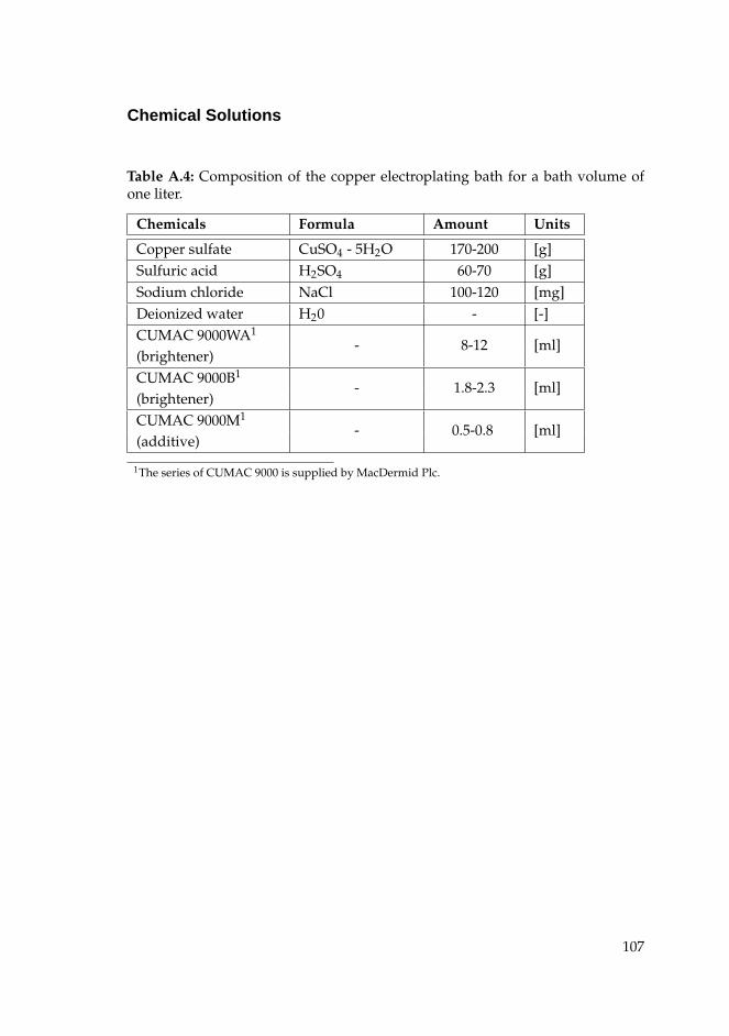
Chemical Solutions
Table A.4: Composition of the copper electroplating bath for a bath volume ofone liter.
Chemicals Formula Amount Units
Copper sulfate CuSO4 - 5H2O 170-200 [g]
Sulfuric acid H2SO4 60-70 [g]
Sodium chloride NaCl 100-120 [mg]
Deionized water H20 - [-]
CUMAC 9000WA1- 8-12 [ml]
(brightener)
CUMAC 9000B1- 1.8-2.3 [ml]
(brightener)
CUMAC 9000M1- 0.5-0.8 [ml]
(additive)
1The series of CUMAC 9000 is supplied by MacDermid Plc.
107

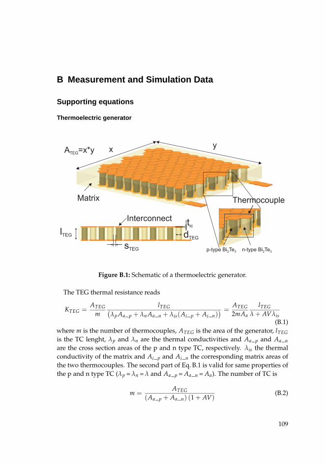
B Measurement and Simulation Data
Supporting equations
Thermoelectric generator
n-type Bi Te2 3p-type Bi Te2 3
lTEG
Matrix
xy
ATEG=x*y
Thermocouple
Interconnect
dTEG
sTEG
tic
Figure B.1: Schematic of a thermoelectric generator.
The TEG thermal resistance reads
KTEG =ATEG
m
lTEG(
λp Aa_p + λn Aa_n + λis(Ai_p + Ai_n)) =
ATEG
2mAa
lTEG
λ + AVλis
(B.1)where m is the number of thermocouples, ATEG is the area of the generator, lTEG
is the TC lenght, λp and λn are the thermal conductivities and Aa_p and Aa_n
are the cross section areas of the p and n type TC, respectively. λis the thermalconductivity of the matrix and Ai_p and Ai_n the corresponding matrix areas ofthe two thermocouples. The second part of Eq. B.1 is valid for same properties ofthe p and n type TC (λp = λn = λ and Aa_p = Aa_n = Aa). The number of TC is
m =ATEG
(Aa_p + Aa_n) (1 + AV)(B.2)
109
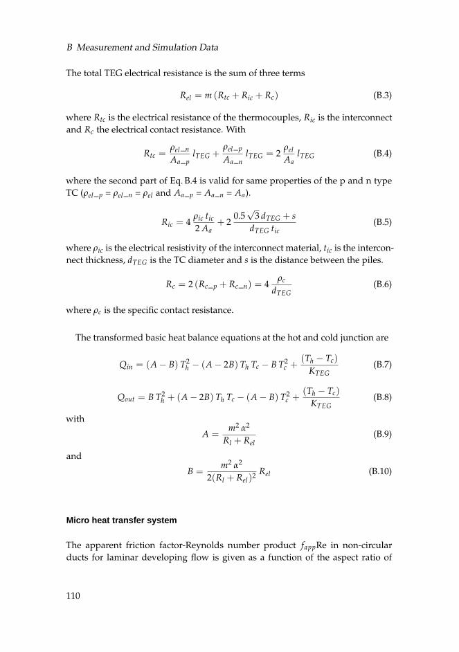
B Measurement and Simulation Data
The total TEG electrical resistance is the sum of three terms
Rel = m (Rtc + Ric + Rc) (B.3)
where Rtc is the electrical resistance of the thermocouples, Ric is the interconnectand Rc the electrical contact resistance. With
Rtc =ρel_n
Aa_plTEG +
ρel_p
Aa_nlTEG = 2
ρel
AalTEG (B.4)
where the second part of Eq. B.4 is valid for same properties of the p and n typeTC (ρel_p = ρel_n = ρel and Aa_p = Aa_n = Aa).
Ric = 4ρic tic
2 Aa+ 2
0.5√
3 dTEG + s
dTEG tic(B.5)
where ρic is the electrical resistivity of the interconnect material, tic is the intercon-nect thickness, dTEG is the TC diameter and s is the distance between the piles.
Rc = 2 (Rc_p + Rc_n) = 4ρc
dTEG(B.6)
where ρc is the specific contact resistance.
The transformed basic heat balance equations at the hot and cold junction are
Qin = (A − B) T2h − (A − 2B) Th Tc − B T2
c +(Th − Tc)
KTEG(B.7)
Qout = B T2h + (A − 2B) Th Tc − (A − B) T2
c +(Th − Tc)
KTEG(B.8)
with
A =m2 α2
Rl + Rel(B.9)
and
B =m2 α2
2(Rl + Rel)2 Rel (B.10)
Micro heat transfer system
The apparent friction factor-Reynolds number product fappRe in non-circularducts for laminar developing flow is given as a function of the aspect ratio of
110
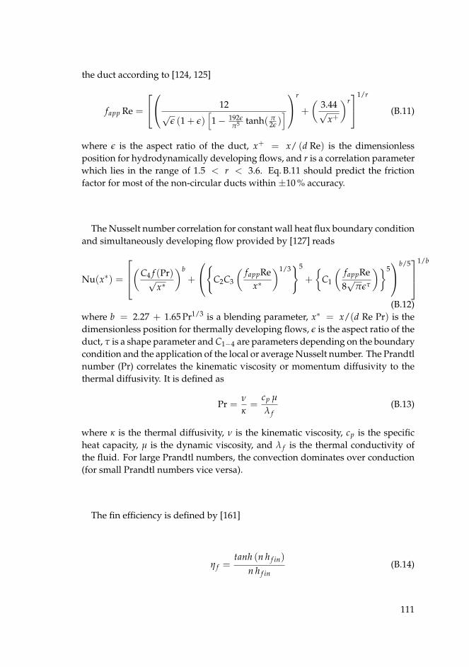
the duct according to [124, 125]
fapp Re =
12√
ǫ (1 + ǫ)[
1 − 192ǫπ5 tanh( π
2ǫ )]
r
+
(
3.44√x+
)r
1/r
(B.11)
where ǫ is the aspect ratio of the duct, x+ = x/ (d Re) is the dimensionlessposition for hydrodynamically developing flows, and r is a correlation parameterwhich lies in the range of 1.5 < r < 3.6. Eq. B.11 should predict the frictionfactor for most of the non-circular ducts within ±10 % accuracy.
The Nusselt number correlation for constant wall heat flux boundary conditionand simultaneously developing flow provided by [127] reads
Nu(x∗) =
(
C4 f (Pr)√x∗
)b
+
C2C3
(
fappRex∗
)1/35
+
C1
(
fappRe
8√
πǫτ
)5
b/5
1/b
(B.12)where b = 2.27 + 1.65 Pr1/3 is a blending parameter, x∗ = x/(d Re Pr) is thedimensionless position for thermally developing flows, ǫ is the aspect ratio of theduct, τ is a shape parameter and C1−4 are parameters depending on the boundarycondition and the application of the local or average Nusselt number. The Prandtlnumber (Pr) correlates the kinematic viscosity or momentum diffusivity to thethermal diffusivity. It is defined as
Pr =ν
κ=
cp µ
λ f(B.13)
where κ is the thermal diffusivity, ν is the kinematic viscosity, cp is the specificheat capacity, µ is the dynamic viscosity, and λ f is the thermal conductivity ofthe fluid. For large Prandtl numbers, the convection dominates over conduction(for small Prandtl numbers vice versa).
The fin efficiency is defined by [161]
η f =tanh (n h f in)
n h f in(B.14)
111
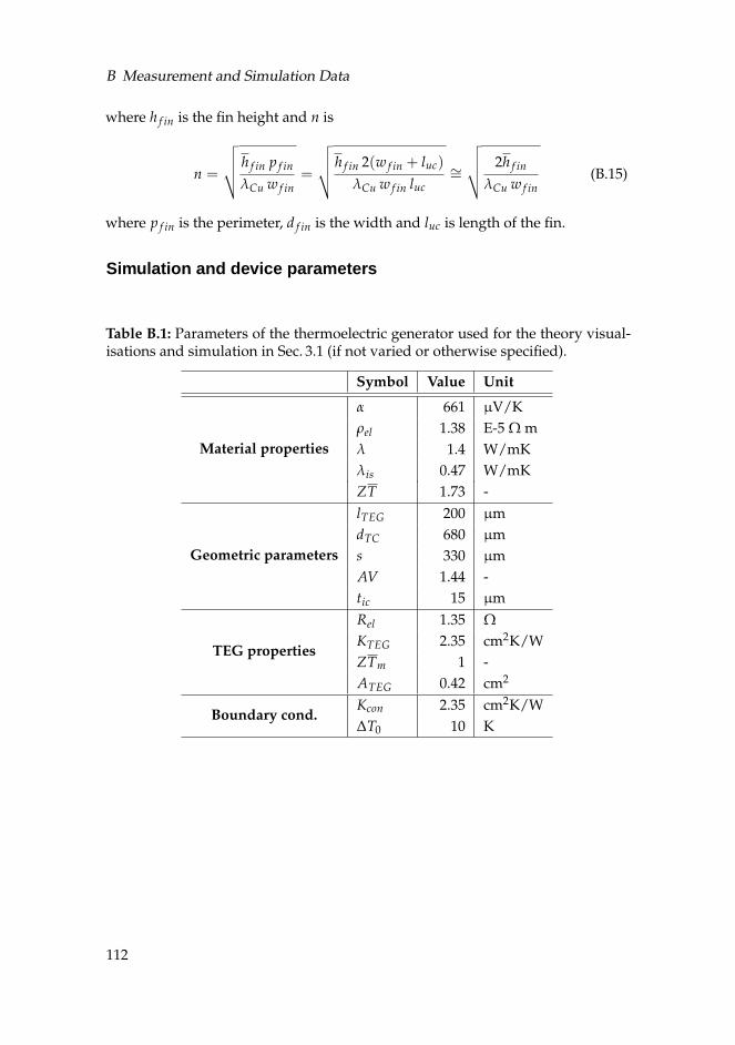
B Measurement and Simulation Data
where h f in is the fin height and n is
n =
√
√
√
√
h f in p f in
λCu w f in=
√
√
√
√
h f in 2(w f in + luc)
λCu w f in luc
∼=
√
√
√
√
2h f in
λCu w f in(B.15)
where p f in is the perimeter, d f in is the width and luc is length of the fin.
Simulation and device parameters
Table B.1: Parameters of the thermoelectric generator used for the theory visual-isations and simulation in Sec. 3.1 (if not varied or otherwise specified).
Symbol Value Unit
Material properties
α 661 µV/K
ρel 1.38 E-5 Ω m
λ 1.4 W/mK
λis 0.47 W/mK
ZT 1.73 -
Geometric parameters
lTEG 200 µm
dTC 680 µm
s 330 µm
AV 1.44 -
tic 15 µm
TEG properties
Rel 1.35 Ω
KTEG 2.35 cm2K/W
ZTm 1 -
ATEG 0.42 cm2
Boundary cond.Kcon 2.35 cm2K/W
∆T0 10 K
112
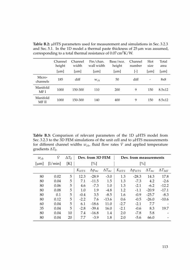
Table B.2: µHTS parameters used for measurement and simulations in Sec. 3.2.3and Sec. 5.1. In the 1D model a thermal paste thickness of 25µm was assumed,corresponding to a total thermal resistance of 0.07 cm2K/W.
Channel Channel Fin/chan. Base/noz. Channel Slot Totalheight width wall width height number size area
[µm] [µm] [µm] [µm] [-] [µm] [µm]
Micro-185 diff wch 50 diff - 8x8
channels
Manifold1000 150-300 110 200 9 150 8.5x12
MF I
Manifold1000 150-300 140 400 9 150 8.5x12
MF II
Table B.3: Comparison of relevant parameters of the 1D µHTS model fromSec. 3.2.3 to the 3D FEM simulations of the unit cell and to µHTS measurementsfor different channel widths wch, fluid flow rates V and applied temperaturegradients ∆T0.
wch V ∆T0 Dev. from 3D FEM Dev. from measurements
[µm] [l/min] [K] [%] [%]
KHTS ∆pmc ∆Tmc KHTS ∆pHTS ∆Tmc ∆TMF
80 0.02 5 12.3 -28.9 -3.0 1.3 -28.3 14.3 17.880 0.04 5 7.1 -11.5 1.5 1.3 -7.3 4.2 -2.680 0.06 5 4.6 -7.3 1.0 1.3 -2.1 -6.2 -12.280 0.08 5 1.0 1.9 -4.8 1.2 -1.1 -20.9 -17.180 0.1 5 -0.4 3.5 -8.5 1.6 -0.9 -25.7 -8.380 0.12 5 -2.2 7.6 -13.6 0.6 -0.5 -26.0 -10.660 0.04 5 6.1 -18.6 11.0 -2.7 -2.1 7.7 -35 0.04 5 -2.8 -39.4 16.0 -2.1 -0.6 8.3 19.780 0.04 10 7.4 -16.8 1.4 2.0 -7.8 5.8 -80 0.04 20 7.7 -3.9 1.8 2.0 -5.6 66.0 -
113
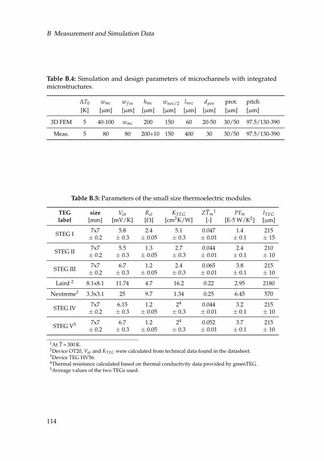
B Measurement and Simulation Data
Table B.4: Simulation and design parameters of microchannels with integratedmicrostructures.
∆T0 wmc w f in hmc wnoz/2 lnoz dpin prot. pitch
[K] [µm] [µm] [µm] [µm] [µm] [µm] [µm] [µm]
3D FEM 5 40-100 wmc 200 150 60 20-50 30/50 97.5/130-390
Meas. 5 80 80 200+10 150 400 30 30/50 97.5/130-390
Table B.5: Parameters of the small size thermoelectric modules.
TEG size Vsb Rel KTEG ZTm1 PFm lTEG
label [mm] [mV/K] [Ω] [cm2K/W] [-] [E-5 W/K2] [µm]
STEG I7x7 5.8 2.4 5.1 0.047 1.4 215± 0.2 ± 0.3 ± 0.05 ± 0.3 ± 0.01 ± 0.1 ± 15
STEG II7x7 5.5 1.3 2.7 0.044 2.4 210± 0.2 ± 0.3 ± 0.05 ± 0.3 ± 0.01 ± 0.1 ± 10
STEG III7x7 6.7 1.2 2.4 0.065 3.8 215± 0.2 ± 0.3 ± 0.05 ± 0.3 ± 0.01 ± 0.1 ± 10
Laird 2 8.1x8.1 11.74 4.7 16.2 0.22 2.95 2180
Nextreme3 3.3x3.1 25 9.7 1.34 0.25 6.45 570
STEG IV7x7 6.15 1.2 24 0.044 3.2 215± 0.2 ± 0.3 ± 0.05 ± 0.3 ± 0.01 ± 0.1 ± 10
STEG V5 7x7 6.7 1.2 24 0.052 3.7 215± 0.2 ± 0.3 ± 0.05 ± 0.3 ± 0.01 ± 0.1 ± 10
1At T = 300 K.2Device OT20, Vsb and KTEG were calculated from technical data found in the datasheet.3Device TEG HV56.4Thermal resistance calculated based on thermal conductivity data provided by greenTEG.5Average values of the two TEGs used.
114
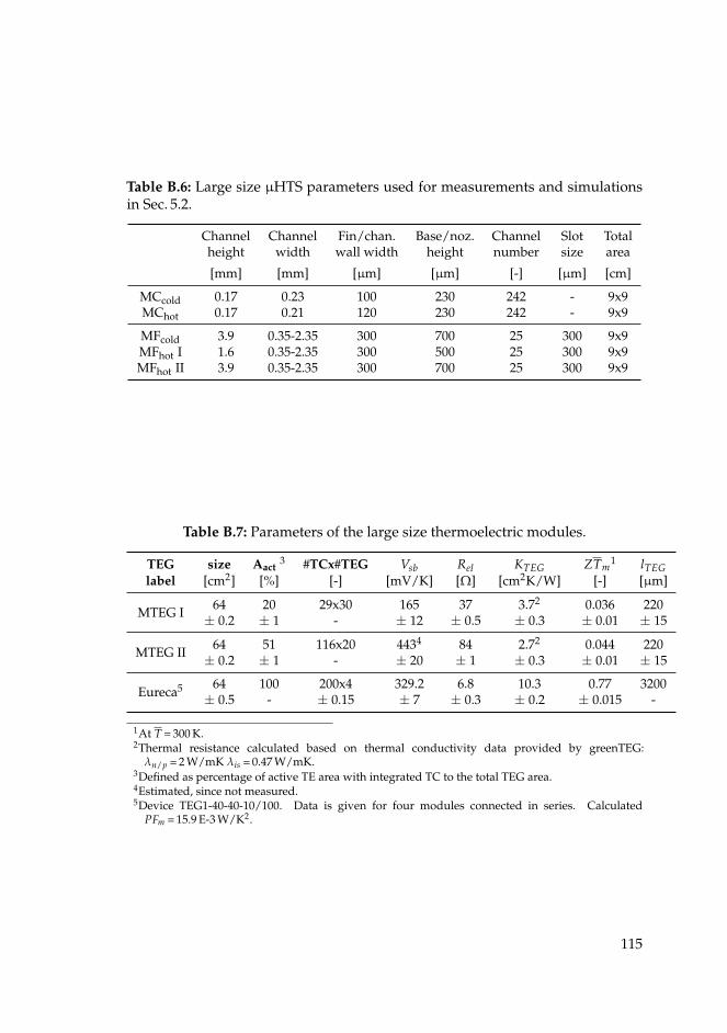
Table B.6: Large size µHTS parameters used for measurements and simulationsin Sec. 5.2.
Channel Channel Fin/chan. Base/noz. Channel Slot Totalheight width wall width height number size area
[mm] [mm] [µm] [µm] [-] [µm] [cm]
MCcold 0.17 0.23 100 230 242 - 9x9MChot 0.17 0.21 120 230 242 - 9x9
MFcold 3.9 0.35-2.35 300 700 25 300 9x9MFhot I 1.6 0.35-2.35 300 500 25 300 9x9MFhot II 3.9 0.35-2.35 300 700 25 300 9x9
Table B.7: Parameters of the large size thermoelectric modules.
TEG size Aact3 #TCx#TEG Vsb Rel KTEG ZTm
1 lTEG
label [cm2] [%] [-] [mV/K] [Ω] [cm2K/W] [-] [µm]
MTEG I64 20 29x30 165 37 3.72 0.036 220
± 0.2 ± 1 - ± 12 ± 0.5 ± 0.3 ± 0.01 ± 15
MTEG II64 51 116x20 4434 84 2.72 0.044 220
± 0.2 ± 1 - ± 20 ± 1 ± 0.3 ± 0.01 ± 15
Eureca5 64 100 200x4 329.2 6.8 10.3 0.77 3200± 0.5 - ± 0.15 ± 7 ± 0.3 ± 0.2 ± 0.015 -
1At T = 300 K.2Thermal resistance calculated based on thermal conductivity data provided by greenTEG:
λn/p = 2 W/mK λis = 0.47 W/mK.3Defined as percentage of active TE area with integrated TC to the total TEG area.4Estimated, since not measured.5Device TEG1-40-40-10/100. Data is given for four modules connected in series. Calculated
PFm = 15.9 E-3 W/K2.
115
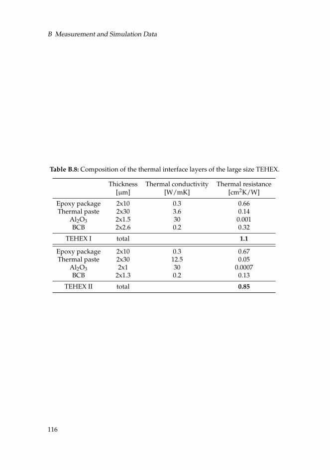
B Measurement and Simulation Data
Table B.8: Composition of the thermal interface layers of the large size TEHEX.
Thickness Thermal conductivity Thermal resistance[µm] [W/mK] [cm2K/W]
Epoxy package 2x10 0.3 0.66Thermal paste 2x30 3.6 0.14
Al2O3 2x1.5 30 0.001BCB 2x2.6 0.2 0.32
TEHEX I total 1.1
Epoxy package 2x10 0.3 0.67Thermal paste 2x30 12.5 0.05
Al2O3 2x1 30 0.0007BCB 2x1.3 0.2 0.13
TEHEX II total 0.85
116
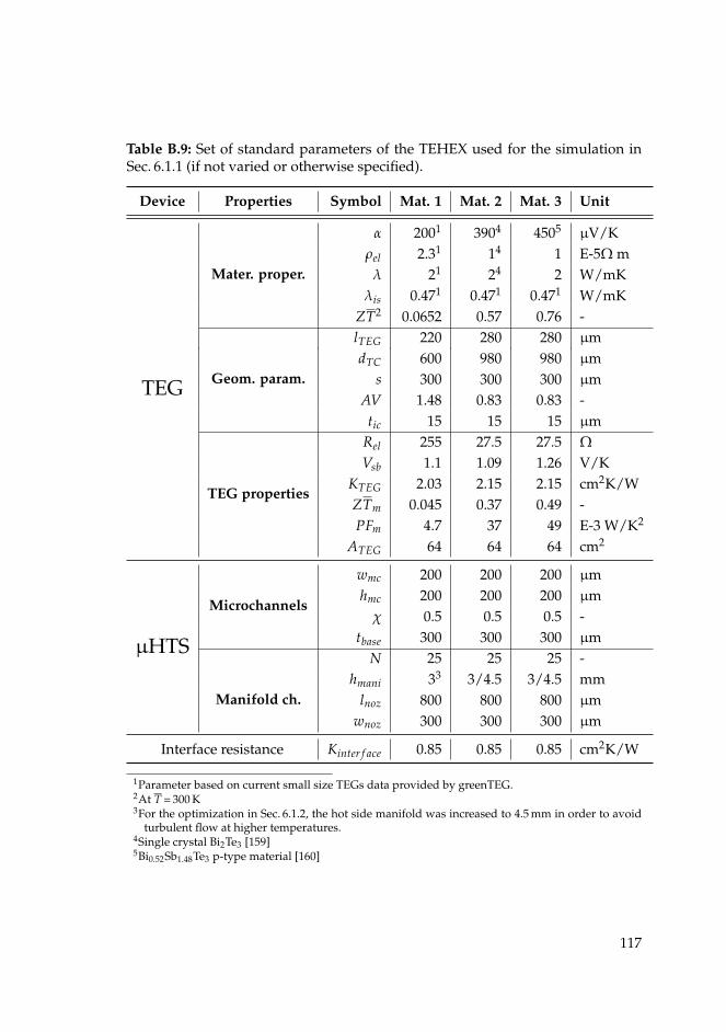
Table B.9: Set of standard parameters of the TEHEX used for the simulation inSec. 6.1.1 (if not varied or otherwise specified).
Device Properties Symbol Mat. 1 Mat. 2 Mat. 3 Unit
TEG
Mater. proper.
α 2001 3904 4505µV/K
ρel 2.31 14 1 E-5Ω m
λ 21 24 2 W/mK
λis 0.471 0.471 0.471 W/mK
ZT2 0.0652 0.57 0.76 -
Geom. param.
lTEG 220 280 280 µm
dTC 600 980 980 µm
s 300 300 300 µm
AV 1.48 0.83 0.83 -
tic 15 15 15 µm
TEG properties
Rel 255 27.5 27.5 Ω
Vsb 1.1 1.09 1.26 V/K
KTEG 2.03 2.15 2.15 cm2K/W
ZTm 0.045 0.37 0.49 -
PFm 4.7 37 49 E-3 W/K2
ATEG 64 64 64 cm2
µHTS
Microchannels
wmc 200 200 200 µm
hmc 200 200 200 µm
χ 0.5 0.5 0.5 -
tbase 300 300 300 µm
Manifold ch.
N 25 25 25 -
hmani 33 3/4.5 3/4.5 mm
lnoz 800 800 800 µm
wnoz 300 300 300 µm
Interface resistance Kinter f ace 0.85 0.85 0.85 cm2K/W
1Parameter based on current small size TEGs data provided by greenTEG.2At T = 300 K3For the optimization in Sec. 6.1.2, the hot side manifold was increased to 4.5 mm in order to avoid
turbulent flow at higher temperatures.4Single crystal Bi2Te3 [159]5Bi0.52Sb1.48Te3 p-type material [160]
117
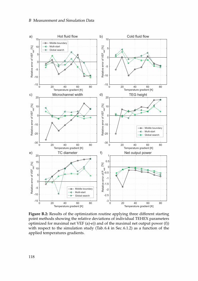
B Measurement and Simulation Data
0 20 40 60 80-30
-20
-10
0
10
20
Temperature gradient [K]
Re
lative
err
or
of
VE
Fn
et[%
]
0 20 40 60 80-15
-10
-5
0
5
10
15
Temperature gradient [K]
Re
lative
err
or
of
VE
Fn
et[%
]
Hot fluid flow
0 20 40 60 80-15
-10
-5
0
5
10
Temperature gradient [K]
Re
lative
err
or
of
VE
Fn
et[%
]
Cold fluid flow
Microchannel width
0 20 40 60 80-15
-10
-5
0
5
10
15
20
Temperature gradient [K]
Re
lative
err
or
of
VE
Fn
et[%
]
0 20 40 60 80-30
-20
-10
0
10
20
Temperature gradient [K]
Re
lative
err
or
of
VE
Fn
et[%
]
TEG height
Middle boundary
Global search
Multi-start
TC diameter
0 20 40 60 80-3
-2.5
-2
-1.5
-1
-0.5
0
0.5
1
Temperature gradient [K]
Re
lative
err
or
of
Pnet
[%]
Net output power
b)a)
c) d)
e) f)
Middle boundary
Global search
Multi-start
Middle boundary
Global search
Multi-start
Figure B.2: Results of the optimization routine applying three different startingpoint methods showing the relative deviations of individual TEHEX parametersoptimized for maximal net VEF (a)-e)) and of the maximal net output power (f))with respect to the simulation study (Tab. 6.4 in Sec. 6.1.2) as a function of theapplied temperatures gradients.
118
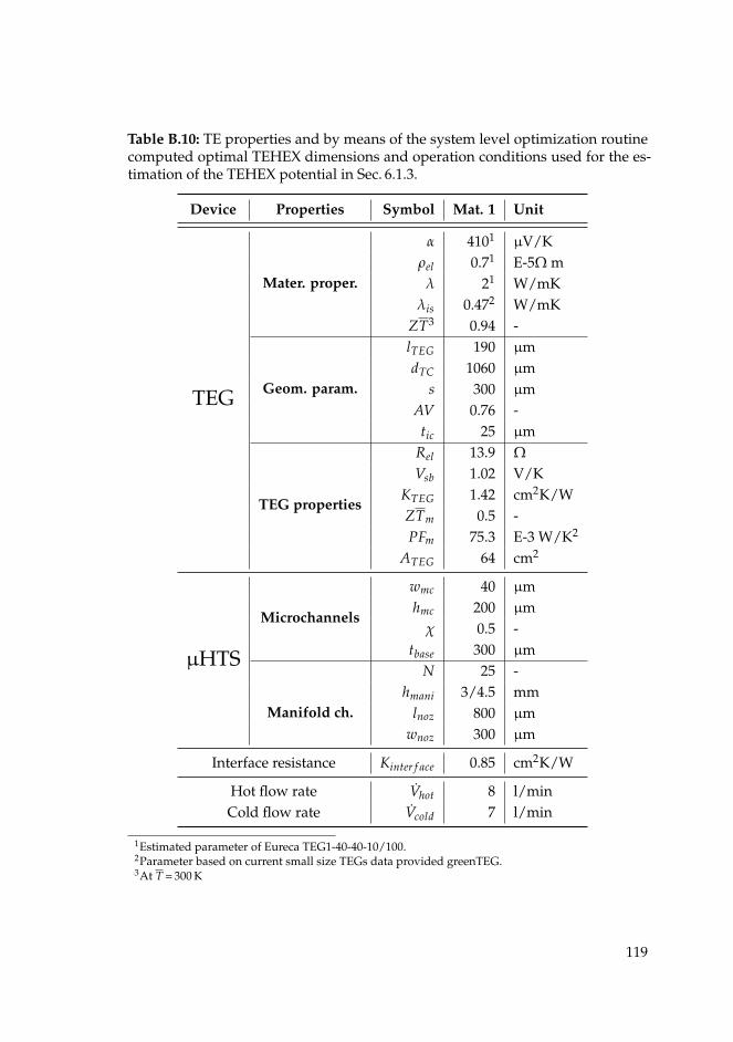
Table B.10: TE properties and by means of the system level optimization routinecomputed optimal TEHEX dimensions and operation conditions used for the es-timation of the TEHEX potential in Sec. 6.1.3.
Device Properties Symbol Mat. 1 Unit
TEG
Mater. proper.
α 4101µV/K
ρel 0.71 E-5Ω m
λ 21 W/mK
λis 0.472 W/mK
ZT3 0.94 -
Geom. param.
lTEG 190 µm
dTC 1060 µm
s 300 µm
AV 0.76 -
tic 25 µm
TEG properties
Rel 13.9 Ω
Vsb 1.02 V/K
KTEG 1.42 cm2K/W
ZTm 0.5 -
PFm 75.3 E-3 W/K2
ATEG 64 cm2
µHTS
Microchannels
wmc 40 µm
hmc 200 µm
χ 0.5 -
tbase 300 µm
Manifold ch.
N 25 -
hmani 3/4.5 mm
lnoz 800 µm
wnoz 300 µm
Interface resistance Kinter f ace 0.85 cm2K/W
Hot flow rate Vhot 8 l/min
Cold flow rate Vcold 7 l/min
1Estimated parameter of Eureca TEG1-40-40-10/100.2Parameter based on current small size TEGs data provided greenTEG.3At T = 300 K
119

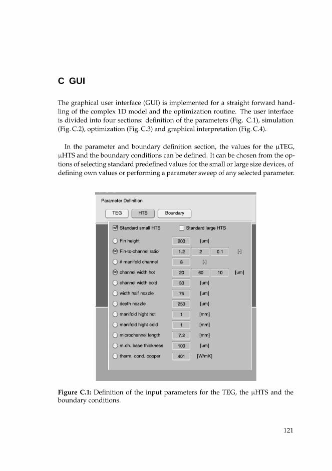
C GUI
The graphical user interface (GUI) is implemented for a straight forward hand-ling of the complex 1D model and the optimization routine. The user interfaceis divided into four sections: definition of the parameters (Fig. C.1), simulation(Fig. C.2), optimization (Fig. C.3) and graphical interpretation (Fig. C.4).
In the parameter and boundary definition section, the values for the µTEG,µHTS and the boundary conditions can be defined. It can be chosen from the op-tions of selecting standard predefined values for the small or large size devices, ofdefining own values or performing a parameter sweep of any selected parameter.
Figure C.1: Definition of the input parameters for the TEG, the µHTS and theboundary conditions.
121
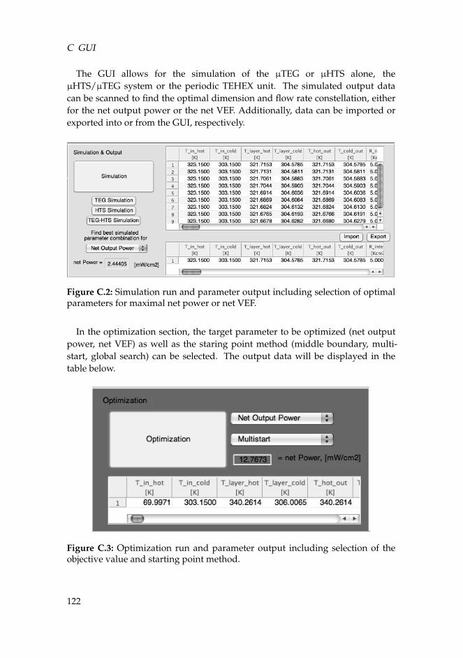
C GUI
The GUI allows for the simulation of the µTEG or µHTS alone, theµHTS/µTEG system or the periodic TEHEX unit. The simulated output datacan be scanned to find the optimal dimension and flow rate constellation, eitherfor the net output power or the net VEF. Additionally, data can be imported orexported into or from the GUI, respectively.
Figure C.2: Simulation run and parameter output including selection of optimalparameters for maximal net power or net VEF.
In the optimization section, the target parameter to be optimized (net outputpower, net VEF) as well as the staring point method (middle boundary, multi-start, global search) can be selected. The output data will be displayed in thetable below.
Figure C.3: Optimization run and parameter output including selection of theobjective value and starting point method.
122
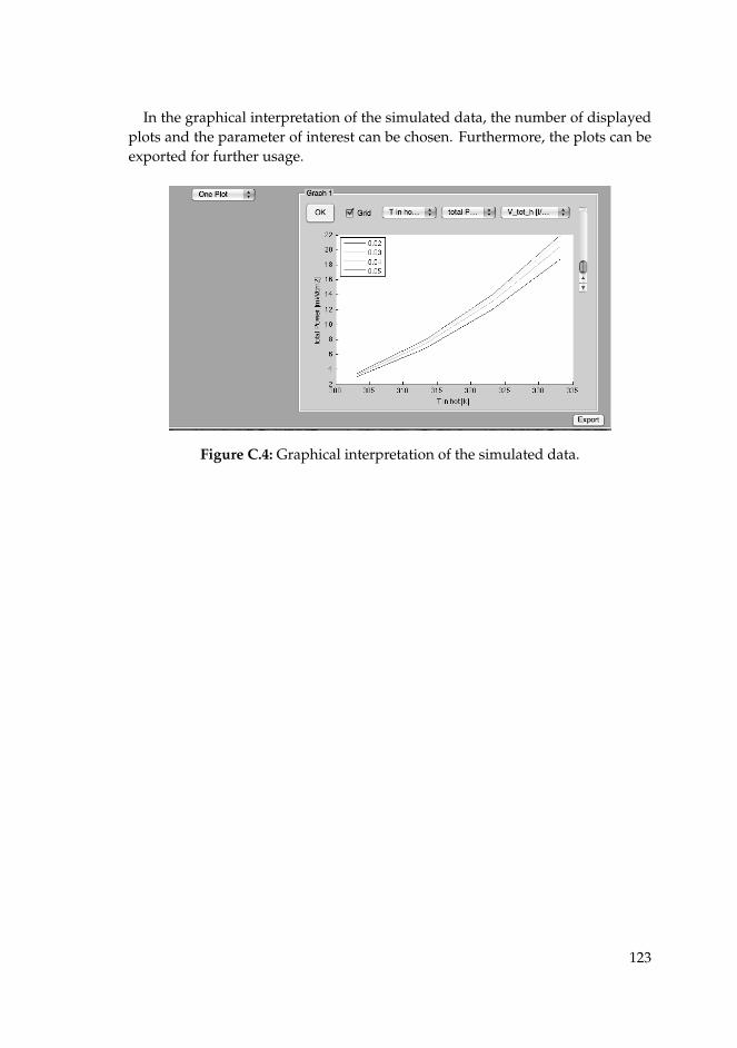
In the graphical interpretation of the simulated data, the number of displayedplots and the parameter of interest can be chosen. Furthermore, the plots can beexported for further usage.
Figure C.4: Graphical interpretation of the simulated data.
123

Bibliography
[1] J. Yagi and T. Akiyama, “Storage of thermal-energy for effective useof waste heat from industries,” Journal of Materials Processing Technology,vol. 48, no. 1-4, pp. 793–804, 1995.
[2] A. S. Rattner and S. Garimella, “Energy harvesting, reuse and upgrade toreduce primary energy usage in the USA,” Energy, vol. 36, no. 10, pp. 6172–6183, 2011.
[3] K. M. Saqr and M. N. Musa, “Critical review of thermoelectrics in modernpower generation applications,” Thermal Science, vol. 13, no. 3, pp. 165–174,2009.
[4] “Annual electric generator report,” U.S. Energy Information Administra-tion, Tech. Rep., 2001.
[5] A. B. Little and S. Garimella, “Comparative assessment of alternative cyclesfor waste heat recovery and upgrade,” Energy, vol. 36, no. 7, pp. 4492–4504,2011.
[6] C. N. Markides, “The role of pumped and waste heat technologies in ahigh-efficiency sustainable energy future for the UK,” Applied Thermal En-
gineering, vol. 53, no. 2, pp. 197–209, 2013.
[7] E. J. Chaisson, “Long-term global heating from energy usage,” Eos, Transac-
tions American Geophysical Union, vol. 89, no. 28, pp. 253–254, 2008.
[8] B. Nordell and B. Gervet, “Global energy accumulation and net heat emis-sion,” International Journal of Global Warming, vol. 1, no. 1-3, pp. 378–391,2009.
[9] G. Min and D. Rowe, “Peltier devices as generators,” in CRC Handbook of
Thermoelectric, 1st ed., ch. 38, D. Rowe, Ed., Boca Raton, FL: CRC Press,1995.
[10] S. B. Riffat and X. L. Ma, “Thermoelectrics: a review of present and poten-tial applications,” Applied Thermal Engineering, vol. 23, no. 8, pp. 913–935,2003.
125
Bibliography
[11] L. E. Bell, “Cooling, heating, generating power, and recovering waste heatwith thermoelectric systems,” Science, vol. 321, no. 5895, pp. 1457–1461,2008.
[12] C. B. Vining, “An inconvenient truth about thermoelectrics,” Nature Mater-
ials, vol. 8, no. 2, pp. 83–85, 2009.
[13] D. Rowe, “Thermoelectric waste heat recovery as a renewable energysource,” International Journal of Innovations in Energy Systems and Power,vol. 1, no. 1, pp. 13–23, 2006.
[14] D. M. Rowe, “Thermoelectric harvesting of low temperature natural/wasteheat,” 9th European Conference on Thermoelectrics (ECT’11), Proceedings, vol.1449, pp. 485–492, 2012.
[15] J. C. Bass, R. J. Campana, and N. B. Elsner, “Thermoelectric generator fordiesel trucks,” 10th International Conference on Thermoelectrics ( ICT’91), Pro-
ceedings, 1991.
[16] J. H. Yang and F. R. Stabler, “Automotive applications of thermoelectricmaterials,” Journal of Electronic Materials, vol. 38, no. 7, pp. 1245–1251, 2009.
[17] M. Kishi, H. Nemoto, T. Hamao, M. Yamamoto, S. Sudou, and M. Mandai,“Micro thermoelectric modules and their application to wristwatches as anenergy source,” 18th International Conference on Thermoelectrics (ICT’99), Pro-
ceedings, pp. 301–307, 1999.
[18] R. J. M. Vullers, R. van Schaijk, I. Doms, C. Van Hoof, and R. Mertens, “Mi-cropower energy harvesting,” Solid-State Electronics, vol. 53, no. 7, pp. 684–693, 2009.
[19] A. Elefsiniotis, D. Samson, T. Becker, and U. Schmid, “Investigation of theperformance of thermoelectric energy harvesters under real flight condi-tions,” Journal of Electronic Materials, vol. 42, no. 7, pp. 2301–2305, 2013.
[20] D. M. Rowe, “Applications of nuclear-powered thermoelectric generatorsin space,” Applied Energy, vol. 40, no. 4, pp. 241–271, 1991.
[21] G. L. Bennett, R. J. Hemler, and A. Schock, “Space nuclear power: An over-view,” Journal of Propulsion and Power, vol. 12, no. 5, pp. 901–910, 1996.
[22] T. R. Lamp and B. D. Donovan, “Unattended power sources for remote,harsh environments,” 29th Intersociety Energy Conversion Engineering Con-
ference, Proceedings, Pts 1-4, pp. 688–693, 1994.
126
Bibliography
[23] T. K. Hunt, R. K. Sievers, and A. C. Patania, “Small AMTEC systems asbattery substitutes,” Space Technology and Applications International Forum,
Pts 1 and 2, vol. 504, pp. 1356–1360, 2000.
[24] R. Venkatasubramanian, E. Siivola, T. Colpitts, and B. O’Quinn, “Thin-film thermoelectric devices with high room-temperature figures of merit,”Nature, vol. 413, no. 6856, pp. 597–602, 2001.
[25] T. C. Harman, P. J. Taylor, M. P. Walsh, and B. E. LaForge, “Quantum dot su-perlattice thermoelectric materials and devices,” Science, vol. 297, no. 5590,pp. 2229–2232, 2002.
[26] J. P. Heremans, M. S. Dresselhaus, L. E. Bell, and D. T. Morelli, “When ther-moelectrics reached the nanoscale,” Nature Nanotechnology, vol. 8, no. 7, pp.471–473, 2013.
[27] W. Glatz, “Development of flexible micro thermoelectric generators,” Dis-sertation, ETH Zurich, Diss ETH No. 17766, 2008.
[28] E. Schwyter, “Fully characterized flexible micro thermoelectric generatorbased on a large scale fabrication approach,” Dissertation, ETH Zurich,Diss ETH No. 20891, 2013.
[29] Y. Lin, Y. Tzeng, M. Dai, C. Liu, L. Liao, H. Chien, Y. Chen, and K. Wang,“Multi-force-field assisted self-assembly process of thermoelectric device,”17th International Conference on Solid-State Sensors, Actuators and Microsys-
tems, Proceedings, pp. 818–821, 2013.
[30] J. W. Stevens, “Optimal design of small DT thermoelectric generation sys-tems,” Energy Conversion and Management, vol. 42, no. 6, pp. 709–720, 2001.
[31] J. R. Couper, W. R. Penney, J. R. Fair, and S. M. Walas, “Heat transfer andheat exchangers,” in Chemical process equipment selection and design, 3rd ed.,ch. 8, pp. 161–221., Waltham, Mass.: Butterworth-Heinemann, 2012.
[32] D. B. Tuckerman and R. F. W. Pease, “High-performance heat sinking forvlsi,” Electron Device Letters, vol. 2, no. 5, pp. 126–129, 1981.
[33] G. L. Morini, “Single-phase convective heat transfer in microchannels: areview of experimental results,” International Journal of Thermal Sciences,vol. 43, no. 7, pp. 631–651, 2004.
[34] B. Agostini, M. Fabbri, J. E. Park, L. Wojtan, J. R. Thome, and B. Michel,“State of the art of high heat flux cooling technologies,” Heat Transfer Engin-
eering, vol. 28, no. 4, pp. 258–281, 2007.
127
Bibliography
[35] C. E. Hunt, C. A. Desmond, D. R. Ciarlo, and W. Benett, “Direct bonding ofmicromachined silicon wafers for laser diode heat exchanger applications,”Journal of Micromechanics and Microengineering, vol. 1, no. 3, pp. 152–156,1991.
[36] E. G. Colgan, B. Furman, M. Gaynes, N. LaBianca, J. H. Magerlein,R. Polastre, R. Bezama, K. Marston, and R. Schmidt, “High performanceand subambient silicon microchannel cooling,” Journal of Heat Transfer-
Transactions of the ASME, vol. 129, no. 8, pp. 1046–1051, 2007.
[37] W. Escher, T. Brunschwiler, B. Michel, and D. Poulikakos, “Experimentalinvestigation of an ultrathin manifold microchannel heat sink for liquid-cooled chips,” Journal of Heat Transfer-Transactions of the ASME, vol. 132,no. 8, p. 081402 (10pp), 2010.
[38] L. Boteler, N. Jankowski, B. Geil, and P. McCluskey, “A micromachinedmanifold microchannel cooler,” ASME International Mechanical Engineering
Congress and Exposition (IMCE2009), Proceedings, vol. 5, no. 43789, pp. 61–68,2009.
[39] G. P. Peterson and C. S. Chang, “Two-phase heat dissipation utilizingporous-channels of high-conductivity material,” Journal of Heat Transfer-
Transactions of the ASME, vol. 120, no. 1, pp. 243–252, 1998.
[40] Y. Peles, A. Kosar, C. Mishra, C. J. Kuo, and B. Schneider, “Forced convect-ive heat transfer across a pin fin micro heat sink,” International Journal of
Heat and Mass Transfer, vol. 48, no. 17, pp. 3615–3627, 2005.
[41] A. Kosar and Y. Peles, “Thermal-hydraulic performance of MEMS-basedpin fin heat sink,” Journal of Heat Transfer-Transactions of the ASME, vol. 128,no. 2, pp. 121–131, 2006.
[42] A. Renfer, M. K. Tiwari, F. Meyer, T. Brunschwiler, B. Michel, and D. Pou-likakos, “Vortex shedding from confined micropin arrays,” Microfluidics
and Nanofluidics, vol. 15, no. 2, pp. 231–242, 2013.
[43] T. Brunschwiler, H. Rothuizen, M. Fabbri, U. Kloter, B. Michel, R. J. Bezama,and G. Natarajan, “Direct liquid jet-impingement cooling with micron-sized nozzle array and distributed return architecture,” 10th Intersociety
Conference on Thermal and Thermomechanical Phenomena in Electronics Systems,
Proceedings, vol. 1 and 2, pp. 196–203, 2006.
[44] W. Escher, B. Michel, and D. Poulikakos, “A novel high performance, ultrathin heat sink for electronics,” International Journal of Heat and Fluid Flow,vol. 31, no. 4, pp. 586–598, 2010.
128
Bibliography
[45] D. M. Rowe, “The NEDO/Cardiff thermoelectric project to economicallyrecover low temperature waste heat,” 17th International Conference on Ther-
moelectrics (ICT’98), Proceedings, pp. 18–24, 1998.
[46] K. Matsuura, D. M. Rowe, A. Tsuyoshi, and G. Min, “Large scale thermo-electric generation of low grade heat,” 10th International Conference on Ther-
moelectrics (ICT’91), Proceedings, pp. 233–241, 1991.
[47] A. Tsuyoshi and K. Matsuura, “A trial manufacture of a thermoelectric gen-erator powered by high-temperature heat transfer medium oil,” Electrical
Engineering in Japan, vol. 141, no. 1, pp. 36–44, 2002.
[48] X. Niu, J. L. Yu, and S. Z. Wang, “Experimental study on low-temperaturewaste heat thermoelectric generator,” Journal of Power Sources, vol. 188,no. 2, pp. 621–626, 2009.
[49] D. T. Crane, J. W. LaGrandeur, F. Harris, and L. E. Bell, “Performance res-ults of a high-power-density thermoelectric generator: Beyond the couple,”Journal of Electronic Materials, vol. 38, no. 7, pp. 1375–1381, 2009.
[50] K. Sasaki, D. Horikawa, and K. Goto, “Consideration of thermoelectricpower generation by using hot spring thermal energy or industrial wasteheat,” 32nd International Conference on Thermoelectrics (ICT’13), 2013.
[51] U. Birkholz, E. Grob, U. Stohrer, K. Voss, D. O. Gruden, and W. Wurster,“Conversion of waste exhaust heat in automobiles using FeSi2 thermoele-ments,” 7th International Conference on Thermoelectric Energy Conversion (ICT
’88), Proceedings, pp. 124–128, 1988.
[52] J. C. Bass, N. B. Elsner, and F. A. Leavitt, “Performance of the 1 kW ther-moelectric generator for Diesel engines,” 13th International Conference on
Thermoelectrics ( ICT’94), Proceedings, no. 316, pp. 295–298, 1995.
[53] J. C. Bass, A. S. Kushch, and N. B. Elsner, “Thermoelectric generator (TEG)for heavy diesel trucks,” 20th International Conference on Thermoelectrics (
ICT’01), Proceedings, pp. 1–5, 2001.
[54] K. Ikoma, M. Munekiyo, K. Furuya, M. Kobayashi, T. Izumi, and K. Shino-hara, “Thermoelectric module and generator for gasoline engine vehicles,”17th International Conference on Thermoelectrics (ICT’98), Proceedings, pp. 464–467, 1998.
[55] K. Matsubara, “Development of a high efficient thermoelectric stack for awaste exhaust heat recovery of vehicles,” 21st International Conference on
Thermoelectrics (ICT’02), Proceedings, pp. 418–423, 2002.
129
Bibliography
[56] D. T. Crane and G. S. Jackson, “Optimization of cross flow heat exchangersfor thermoelectric waste heat recovery,” Energy Conversion and Management,vol. 45, no. 9-10, pp. 1565–1582, 2004.
[57] E. F. Thacher, B. T. Helenbrook, M. A. Karri, and C. J. Richter, “Testing of anautomobile exhaust thermoelectric generator in a light truck,” Proceedings
of the Institution of Mechanical Engineers Part D-Journal of Automobile Engin-
eering, vol. 221, no. D1, pp. 95–107, 2007.
[58] X. L. Gou, H. Xiao, and S. W. Yang, “Modeling, experimental study andoptimization on low-temperature waste heat thermoelectric generator sys-tem,” Applied Energy, vol. 87, no. 10, pp. 3131–3136, 2010.
[59] C. T. Hsu, D. J. Yao, K. J. Ye, and B. Yu, “Renewable energy of waste heat re-covery system for automobiles,” Journal of Renewable and Sustainable Energy,vol. 2, no. 1, 2010.
[60] C. R. Kumar, A. Sonthalia, and R. Goel, “Experimental study on waste heatrecovery from an internal combustion engine using thermoelectric techno-logy,” Thermal Science, vol. 15, no. 4, pp. 1011–1022, 2011.
[61] L. I. Anatychuk, Y. Y. Rozver, and D. D. Velichuk, “Thermoelectric gen-erator for a stationary diesel plant,” Journal of Electronic Materials, vol. 40,no. 5, pp. 1206–1208, 2011.
[62] L. I. Anatychuk and R. V. Kuz, “Computer design and test results of auto-motive thermoelectric generator,” in Thermoelectrics Goes Automotive, vol.2nd, pp. 191–208, D. Jänsch, Ed., Renningen: expert verlag, 2011.
[63] L. I. Anatychuk, O. J. Luste, and R. V. Kuz, “Theoretical and experimentalstudy of thermoelectric generators for vehicles,” Journal of Electronic Mater-
ials, vol. 40, no. 5, pp. 1326–1331, 2011.
[64] M. Mori, T. Yamagami, M. Sorazawa, T. Miyabe, S. Takahashi, and T. Har-aguchi, “Fuel economy simulation of series hybrid utilizing thermoelec-tric heat recovery system,” in Thermoelectrics Goes Automotive, pp. 154–167,D. Jänsch, Ed., Renningen: expert verlag, 2011.
[65] D. Crane, L. Bell, and J. LaGrandeur, “Progress report on vehicular wasteheat recovery using a cylindrical thermoelectric generator,” in Thermoelec-
trics Goes Automotive, vol. 2nd, pp. 83–91, D. Jänsch, Ed., Renningen: expertverlag, 2011.
[66] D. T. Crane, C. R. Koripella, and V. Jovovic, “Validating steady-state andtransient modeling tools for high-power-density thermoelectric generat-ors,” Journal of Electronic Materials, vol. 41, no. 6, pp. 1524–1534, 2012.
130
Bibliography
[67] D. Crane, J. LaGrandeur, V. Jovovic, M. Ranalli, M. Adldinger, E. Poliquin,J. Dean, D. Kossakovski, B. Mazar, and C. Maranville, “TEG on-vehicle per-formance and model validation and what it means for further TEG devel-opment,” Journal of Electronic Materials, vol. 42, no. 7, pp. 1582–1591, 2013.
[68] T. Kajikawa, “Present state of R&D on thermoelectric technology in Japan,”20th International Conference on Thermoelectrics (ICT’01), Proceedings, pp. 49–56, 2001.
[69] H. H. Braess and U. Seiffert, Vieweg Handbuch Kraftfahrzeugtechnik, 6th ed.,Springer DE, 2011.
[70] J. L. Creveling, “Means for utilizing waste energy,” US Patent US1 118 269A, 1914.
[71] A. J. Neild, “Portable thermoelectric generators,” SAE-645A (Society of Auto-
motive Engineers), 1963.
[72] D. Jaensch, Thermoelectric Goes Automotive, 2nd ed., p. 295., Renningen: ex-pert verlag, 2011.
[73] J. Salvador, “Challenges for future implementation of thermoelectric wasteheat recovery,” 32nd International Conference on Thermoelectrics (ICT’13),2013.
[74] M. Linde, B. Mazar, A. Eder, S. Neugebauer, and R. Brueck, “Der AGR-TEG:Ein Pilotprojekt auf dem Weg zur Industrialisierung der Thermoelektrikim Kraftfahrzeug,” in Thermoelectrics Goes Automotive, vol. 2nd, pp. 71–82,D. Jänsch, Ed., Renningen: expert verlag, 2011.
[75] J. Yang and F. R. Stabler, “Automotive applications of thermoelectric ma-terials,” in Thermoelectrics and its energy harvesting. Modules, systems, and ap-
plications in thermoelectrics, D. M. Rowe, Ed., Boca Raton, FL: CRC Press,2012.
[76] D. B. Heymann, C. D. Meyer, N. R. Jankowski, and B. C. Morgan, “Model-ing the system impact of cooling performance on a compact thermoelectricgenerator,” PowerMEMS 2009, Proceedings, 2009.
[77] D. Astrain, J. G. Vian, A. Martinez, and A. Rodriguez, “Study of the influ-ence of heat exchangers’ thermal resistances on a thermoelectric generationsystem,” Energy, vol. 35, no. 2, pp. 602–610, 2010.
[78] K. Yazawa and A. Shakouri, “Cost-efficiency trade-off and the designof thermoelectric power generators,” Environmental Science & Technology,vol. 45, no. 17, pp. 7548–7553, 2011.
131
Bibliography
[79] A. Rezania and L. A. Rosendahl, “Evaluating thermoelectric power gen-eration device performance using a rectangular microchannel heat sink,”Journal of Electronic Materials, vol. 40, no. 5, pp. 481–488, 2011.
[80] A. Rezania and L. A. Rosendahl, “Thermal effect of a thermoelectric gener-ator on parallel microchannel heat sink,” Energy, vol. 37, no. 1, pp. 220–227,2012.
[81] A. Rezania, L. A. Rosendahl, and S. J. Andreasen, “Experimental investig-ation of thermoelectric power generation versus coolant pumping powerin a microchannel heat sink,” International Communications in Heat and Mass
Transfer, vol. 39, no. 8, pp. 1054–1058, 2012.
[82] B. Mathew, B. Jakub-Wood, E. Ogbonnaya, and L. Weiss, “Investigation ofa MEMS-based capillary heat exchanger for thermal harvesting,” Interna-
tional Journal of Heat and Mass Transfer, vol. 58, no. 1-2, pp. 492–502, 2013.
[83] T. J. Seebeck, Magnetische Polarisation der Metalle und Erze durch Temperatur-
Differenz, p. 120., Leipzig: Wilhelm Engelmann, 1823.
[84] S. Middelhoek and S. Audet, Silicon sensors, ser. Microelectronics and signalprocessing, p. 376., London: Academic Press In, 1989.
[85] R. Pelster, R. Pieper, and I. Huettl, “Thermospannung - Viel genutzt undfast immer falsch erklärt,” in PhyDid, vol. 1, pp. 10–22, 2005.
[86] M. Cutler and N. F. Mott, “Observation of Anderson localization in an elec-tron gas,” Physical Review, vol. 181, no. 3, pp. 1336–1340, 1969.
[87] H. Fritzsch, “General expression for thermoelectric power,” Solid State Com-
munications, vol. 9, no. 21, pp. 1813–1815, 1971.
[88] N. W. Ashcroft and N. D. Mermin, Solid state physics, 1st ed., p. 826., NewYork: Holt, Rinehart and Winston, 1976.
[89] M. Freunek, “Untersuchung der Thermoelektrik zur Energieversorgungautarkter Systeme,” Dissertation, University Freiburg, 2010.
[90] A. F. Ioffe, Semiconductor Thermoelements and Thermoelectric Cooling., Lon-don: Infosearch, ltd, 1957.
[91] L. D. Hicks and M. S. Dresselhaus, “Effect of quantum-well structures onthe thermoelectric figure of merit,” Physical Review B, vol. 47, no. 19, pp.12 727–12 731, 1993.
132
Bibliography
[92] L. D. Hicks and M. S. Dresselhaus, “Thermoelectric figure of merit of a one-dimensional conductor,” Physical Review B, vol. 47, no. 24, pp. 16 631–16 634,1993.
[93] L. D. Hicks, T. C. Harman, X. Sun, and M. S. Dresselhaus, “Experimentalstudy of the effect of quantum-well structures on the thermoelectric figureof merit,” Physical Review B, vol. 53, no. 16, pp. 10 493–10 496, 1996.
[94] Y. M. Lin, X. Z. Sun, and M. S. Dresselhaus, “Theoretical investigation ofthermoelectric transport properties of cylindrical Bi nanowires,” Physical
Review B, vol. 62, no. 7, pp. 4610–4623, 2000.
[95] J. P. Heremans, C. M. Thrush, D. T. Morelli, and M. C. Wu, “Thermoelectricpower of bismuth nanocomposites,” Physical Review Letters, vol. 88, no. 21,2002.
[96] K. F. Hsu, S. Loo, F. Guo, W. Chen, J. S. Dyck, C. Uher, T. Hogan, E. K.Polychroniadis, and M. G. Kanatzidis, “Cubic AgPbmSbTe2+m: Bulk ther-moelectric materials with high figure of merit,” Science, vol. 303, no. 5659,pp. 818–821, 2004.
[97] D. M. Rowe, “Theoretical optimization of thermoelectric figure of merit ofheavily doped hot-pressed germanium-silicon alloys,” Journal of Physics F-
Metal Physics, vol. 7, no. 13, pp. 1843–1846, 1974.
[98] G. A. Slack and M. A. Hussain, “The maximum possible conversion effi-ciency of silicon-germanium thermoelectric generators,” Journal of Applied
Physics, vol. 70, no. 5, pp. 2694–2718, 1991.
[99] D. G. Cahill, W. K. Ford, K. E. Goodson, G. D. Mahan, A. Majumdar, H. J.Maris, R. Merlin, and P. Sr, “Nanoscale thermal transport,” Journal of Ap-
plied Physics, vol. 93, no. 2, pp. 793–818, 2003.
[100] J. Yang, W. Zhang, S. Q. Bai, Z. Mei, and L. D. Chen, “Dual-frequency reson-ant phonon scattering in BaxRyCo4Sb12 (R=La, Ce, and Sr),” Applied Physics
Letters, vol. 90, no. 19, 2007.
[101] A. I. Hochbaum, R. K. Chen, R. D. Delgado, W. J. Liang, E. C. Garnett,M. Najarian, A. Majumdar, and P. D. Yang, “Enhanced thermoelectric per-formance of rough silicon nanowires,” Nature, vol. 451, no. 7175, pp. 163–167, 2008.
[102] K. Biswas, J. Q. He, I. D. Blum, C. I. Wu, T. P. Hogan, D. N. Seidman,V. P. Dravid, and M. G. Kanatzidis, “High-performance bulk thermoelec-trics with all-scale hierarchical architectures,” Nature, vol. 489, no. 7416, pp.414–418, 2012.
133
Bibliography
[103] J. P. Heremans, V. Jovovic, E. S. Toberer, A. Saramat, K. Kurosaki, A. Char-oenphakdee, S. Yamanaka, and G. J. Snyder, “Enhancement of thermoelec-tric efficiency in PbTe by distortion of the electronic density of states,” Sci-
ence, vol. 321, no. 5888, pp. 554–557, 2008.
[104] K. Matsuura and D. Rowe, “Low-temperature heat conversion,” in CRC
Handbook of Thermoelectric, 1st ed., ch. 44, D. Rowe, Ed., Boca Raton, FL:CRC Press, 1995.
[105] C. Wu, “Analysis of waste-heat thermoelectric power generators,” Applied
Thermal Engineering, vol. 16, no. 1, pp. 63–69, 1996.
[106] M. Strasser, “Entwicklung und Charakterisierung mikrostrukturierter ther-moelektrischer Generatoren in Silizium-Halbleitertechnologie,” Disserta-tion, Technische Universität München, 2002.
[107] L. G. Chen, J. Z. Gong, F. R. Sun, and C. Wu, “Effect of heat transfer on theperformance of thermoelectric generators,” International Journal of Thermal
Sciences, vol. 41, no. 1, pp. 95–99, 2002.
[108] M. Strasser, R. Aigner, C. Lauterbach, T. F. Sturm, M. Franosch, andG. Wachutka, “Micromachined CMOS thermoelectric generators as on-chippower supply,” Sensors and Actuators A: Physical, vol. 114, no. 2-3, pp. 362–370, 2004.
[109] M. Freunek, M. Muller, T. Ungan, W. Walker, and L. M. Reindl, “Newphysical model for thermoelectric generators,” Journal of Electronic Mater-
ials, vol. 38, no. 7, pp. 1214–1220, 2009.
[110] Y. Apertet, H. Ouerdane, O. Glavatskaya, C. Goupil, and P. Lecoeur,“Optimal working conditions for thermoelectric generators with realisticthermal coupling,” EPL, vol. 97, no. 2, 2012.
[111] C. N. Rollinger and J. E. Sunderland, “The performance of a convectivelycooled thermoelement used for power generation,” Solid-State Electronics,vol. 3, no. 3-4, pp. 268–277, 1961.
[112] B. R. West, “A method for designing a thermoelectric generator basedon the thermal characteristics of the device,” Advanced Energy Conversion,vol. 2, pp. 209–218, 1962.
[113] M. Strasser, R. Aigner, M. Franosch, and G. Wachutka, “Miniaturized ther-moelectric generators based on poly-Si and polySiGe surface micromachin-ing,” Sensors and Actuators A: Physical, vol. 97-8, pp. 535–542, 2002.
134
Bibliography
[114] W. Glatz, S. Muntwyler, and C. Hierold, “Optimization and fabrication ofthick flexible polymer based micro thermoelectric generator,” Sensors and
Actuators A: Physical, vol. 132, no. 1, pp. 337–345, 2006.
[115] J. Stevens, “Optimized thermal design of small DT thermoelectric generat-ors,” 34th Intersociety Energy Conversion Engineering Conference, Proceedings,pp. 1999–01–2564, 1999.
[116] Y. Ma, Q. Hao, B. Poudel, Y. C. Lan, B. Yu, D. Z. Wang, G. Chen, and Z. F.Ren, “Enhanced thermoelectric figure-of-merit in p-type nanostructuredbismuth antimony tellurium alloys made from elemental chunks,” Nano
Letters, vol. 8, no. 8, pp. 2580–2584, 2008.
[117] W. Kim, J. Zide, A. Gossard, D. Klenov, S. Stemmer, A. Shakouri, andA. Majumdar, “Thermal conductivity reduction and thermoelectric figureof merit increase by embedding nanoparticles in crystalline semiconduct-ors,” Physical Review Letters, vol. 96, no. 4, 2006.
[118] T. C. Harman, M. P. Walsh, B. E. Laforge, and G. W. Turner, “Nanostruc-tured thermoelectric materials,” Journal of Electronic Materials, vol. 34, no. 5,pp. L19–L22, 2005.
[119] D. Narducci, “Do we really need high thermoelectric figures of merit? acritical appraisal to the power conversion efficiency of thermoelectric ma-terials,” Applied Physics Letters, vol. 99, no. 10, 2011.
[120] F. Incropera, D. P. Dewitt, T. L. Bergman, and A. S. Lavine, Fundamentals
of heat and mass transfer, 6th ed., p. 997., Hoboken, NJ: John Wiley & Sons,2007.
[121] R. W. Hanks and H. C. Ruo, “Laminar-turbulent transition in ducts ofrectangular cross section,” Industrial & Engineering Chemistry Fundamentals,vol. 5, no. 4, pp. 558–561, 1966.
[122] R. K. Shah and A. L. London, Laminar Flow Forced Convection in
Ducts.Academic Press, New York, 1978.
[123] M. M. Yovanovich and Y. S. Muzychka, “Solutions of poisson equationwithin singly and doubly connected domains,” AIAA Paper, vol. 97-3880,pp. 1–11, 1997.
[124] Y. S. Muzychka and M. M. Yovanovich, “Modeling friction factors in non-circular ducts for developing laminar flow,” AIAA Paper, vol. 98-2492, pp.1–12, 1998.
135
Bibliography
[125] Y. S. Muzychka and M. M. Yovanovich, “Pressure drop in laminar develop-ing flow in noncircular ducts: A scaling and modeling approach,” Journal
of Fluids Engineering-Transactions of the ASME, vol. 131, no. 11, 2009.
[126] L. C. Burmeister, Convective heat transfer, 2nd ed., p. 619., New York: Wiley,1993.
[127] Y. S. Muzychka and M. M. Yovanovich, “Laminar forced convection heattransfer in the combined entry region of non-circular ducts,” Journal of Heat
Transfer-Transactions of the ASME, vol. 126, no. 1, pp. 54–61, 2004.
[128] J. Pfahler, J. Harley, H. Bau, and J. Zemel, “Liquid transport in micron andsubmicron channels,” Sensors and Actuators A: Physical, vol. 22, no. 1-3, pp.431–434, 1989.
[129] W. Urbanek, J. N. Zemel, and H. H. Bau, “An investigation of the temper-ature dependence of Poiseuille numbers in microchannel flow,” Journal of
Micromechanics and Microengineering, vol. 3, no. 4, pp. 206–209, 1993.
[130] I. Papautsky, J. Brazzle, T. Ameel, and A. B. Frazier, “Laminar fluid beha-vior in microchannels using micropolar fluid theory,” Sensors and Actuators
A: Physical, vol. 73, no. 1-2, pp. 101–108, 1999.
[131] G. M. Mala and D. Q. Li, “Flow characteristics of water in microtubes,”International Journal of Heat and Fluid Flow, vol. 20, no. 2, pp. 142–148, 1999.
[132] W. L. Qu, G. M. Mala, and D. Q. Li, “Pressure-driven water flows intrapezoidal silicon microchannels,” International Journal of Heat and Mass
Transfer, vol. 43, no. 3, pp. 353–364, 2000.
[133] Z. Y. Guo and Z. X. Li, “Size effect on microscale single-phase flow andheat transfer,” International Journal of Heat and Mass Transfer, vol. 46, no. 1,pp. 149–159, 2003.
[134] G. L. Morini, “Viscous heating in liquid flows in micro-channels,” Interna-
tional Journal of Heat and Mass Transfer, vol. 48, no. 17, pp. 3637–3647, 2005.
[135] C. L. Ren and D. Q. Li, “Electroviscous effects on pressure-driven flow ofdilute electrolyte solutions in small microchannels,” Journal of Colloid and
Interface Science, vol. 274, no. 1, pp. 319–330, 2004.
[136] X. F. Peng, G. P. Peterson, and B. X. Wang, “Frictional flow characteristicsof water flowing through rectangular microchannels,” Experimental Heat
Transfer, vol. 7, no. 4, pp. 249–264, 1994.
136
Bibliography
[137] X. N. Jiang, Z. Y. Zhou, X. Y. Huang, and C. Y. Liu, “Laminar flow throughmicrochannels used for microscale cooling systems,” 1st Electronic Pack-
aging Technology Conference 1997, Proceedings, pp. 119–122, 1997.
[138] B. Xu, K. T. Ooi, N. T. Wong, and W. K. Choi, “Experimental investigationof flow friction for liquid flow in microchannels,” International Communica-
tions in Heat and Mass Transfer, vol. 27, no. 8, pp. 1165–1176, 2000.
[139] P. Gao, S. Le Person, and M. Favre-Marinet, “Scale effects on hydrodynam-ics and heat transfer in two-dimensional mini and microchannels,” Interna-
tional Journal of Thermal Sciences, vol. 41, no. 11, pp. 1017–1027, 2002.
[140] J. Judy, D. Maynes, and B. W. Webb, “Characterization of frictional pressuredrop for liquid flows through microchannels,” International Journal of Heat
and Mass Transfer, vol. 45, no. 17, pp. 3477–3489, 2002.
[141] D. Liu and S. V. Garimella, “Investigation of liquid flow in microchannels,”Journal of Thermophysics and Heat Transfer, vol. 18, no. 1, pp. 65–72, 2004.
[142] K. V. Sharp and R. J. Adrian, “Transition from laminar to turbulent flow inliquid filled microtubes,” Experiments in Fluids, vol. 36, no. 5, pp. 741–747,2004.
[143] M. J. Kohl, S. I. Abdel-Khalik, S. M. Jeter, and D. L. Sadowski, “An experi-mental investigation of microchannel flow with internal pressure measure-ments,” International Journal of Heat and Mass Transfer, vol. 48, no. 8, pp.1518–1533, 2005.
[144] M. Akbari, D. Sinton, and M. Bahrami, “Pressure drop in rectangular mi-crochannels as compared with theory based on arbitrary cross section,”Journal of Fluids Engineering-Transactions of the ASME, vol. 131, no. 4, 2009.
[145] R. Baviere, F. Ayela, S. Le Person, and M. Favre-Marinet, “Experimentalcharacterization of water flow through smooth rectangular microchannels,”Physics of Fluids, vol. 17, no. 9, 2005.
[146] W. Escher, “Ultra thin high efficiency heat sinks with water or nanofluidfor electronics,” Dissertation, ETH Zurich, Diss ETH No. 8667, 2009.
[147] G. J. Michna, E. A. Browne, Y. Peles, and M. K. Jensen, “Single-phase micro-scale jet stagnation point heat transfer,” Journal of Heat Transfer-Transactions
of the ASME, vol. 131, no. 11, p. 111402 (8pp), 2009.
[148] S. G. Kandlikar, “Single-phase liquid flow in minichannels and microchan-nels,” in Heat transfer and fluid flow in minichannels and microchannels, 1st ed.,
137
Bibliography
ch. 3, pp. 87–136., Amsterdam, Netherlands ; San Diego, CA ; Oxford, UK:Elsevier, 2006.
[149] W. L. Qu and I. Mudawar, “Experimental and numerical study of pressuredrop and heat transfer in a single-phase micro-channel heat sink,” Interna-
tional Journal of Heat and Mass Transfer, vol. 45, no. 12, pp. 2549–2565, 2002.
[150] W. Bohl and W. Elmendorf, “Inkompressible Strömungen,” in Technische
Strömungslehre, 13th ed., ch. 4., Würzburg: Vogel Business Media, 2005.
[151] N. Wojtas and C. Hierold, “Microfluidic heat transfer systems optimizedfor thermoelectric heat exchangers,” 17th International Conference on Solid-
State Sensors, Actuators and Microsystems, Proceedings, pp. 1368–1371, 2013.
[152] F. Kreith, R. M. Manglik, and M. Bohn, Principles of heat transfer, 7th ed., p.696., Stamford, CT: Cengage Learning, 2011.
[153] N. Wojtas, E. Schwyter, W. Glatz, S. Kühne, W. Escher, and C. Hierold,“Power enhancement of micro thermoelectric generators by microfluidicheat transfer packaging,” Sensors and Actuators A: Physical, vol. 188, pp. 289–295, 2012.
[154] F. Umbrecht, D. Muller, F. Gattiker, C. M. Boutry, J. Neuenschwander,U. Sennhauser, and C. Hierold, “Solvent assisted bonding of polymethyl-methacrylate: Characterization using the response surface methodology,”Sensors and Actuators A: Physical, vol. 156, no. 1, pp. 121–128, 2009.
[155] UKAS, “The expression of uncertainty and confidence in measurement,”2007.
[156] N. Wojtas, L. Ruthemann, W. Glatz, and C. Hierold, “Optimized thermalcoupling of micro thermoelectric generators for improved output perform-ance,” Renewable Energy, vol. 60, pp. 746–753, 2013.
[157] N. Wojtas, M. Grab, W. Glatz, and C. Hierold, “Stacked micro heat ex-change system for optimized thermal coupling of microTEGs,” Journal of
Electronic Materials, vol. 42, no. 7, pp. 2103–2109, 2013.
[158] H. Schmid, “Less emissions through waste heat recovery,” Green Ship Tech-
nology Conference ’04, Proceedings, 2004.
[159] H. J. Goldsmid, A. R. Sheard, and D. A. Wright, “The performance of bis-muth telluride thermojunctions,” British Journal of Applied Physics, vol. 9,no. 9, pp. 365–370, 1958.
138

Bibliography
[160] W. J. Xie, X. F. Tang, Y. G. Yan, Q. J. Zhang, and T. M. Tritt, “Unique nano-structures and enhanced thermoelectric performance of melt-spun BiSbTealloys,” Applied Physics Letters, vol. 94, no. 10, 2009.
[161] J. I. Lienhard and J. V. Lienhard, “Analysis of heat conduction and somesteady one-dimensional problems,” in A heat transfer textbook, ch. 4, pp. 141–191., Cambridge, Massachusetts: Phlogiston Press, 2008.
139


Acknowledgement
I would like to thank Prof. Hierold for offering me the opportunity to conductthis PhD thesis in the Micro and Nanosystems group at ETH Zürich. Further-more, I would like to thank my co-referee Prof. Poulikakos for the final review ofthis work.
Many thanks for interesting discussion, support and great company go toall the current and previous members of the MNS group. In particular specialthanks go to Etienne Schwyter who introduced me to the topic of thermoelec-tricity during my master thesis and has also helped me with interesting inputsduring the course of the project. I am very much obliged to Stéphane Kühnefor valuable processing advices, help with the measurement setup and proofreading this thesis. Also the processing support, interesting discussions andcontinuous ’funny’ jokes from Yunjia Li are greatly appreciated. Furthermore, Iwould like to thank Emine Cagin for great scientific and personal conversationsand for proofreading many English reports, including main parts of this PhDthesis. I really enjoyed sharing the office with her.
Also many thanks go to the greenTEG team for providing me with TEGsamples, processing opportunities and great support. Special thanks go ThomasHelbling for valuable scientific inputs, Florian Umbrecht for building the largescale measurement setup, Michele Zahner for the help with the large scalemicrochannel fabrication and Wulf Glatz for initiating the TEG project with hiswork on flexible micro thermoelectric generators.
I am very much indebted to all my master, semester and bachelor thesisstudents who greatly contributed to the success of this project: Barbara Schaffner,Davud Sadihov, Floria Ottonello, Franziska Ryser, Gion-Andri Büsser, LukasRüthemann, Maarten Flink, Martina Grab, Patrick Streit, Samuel Ruckstuhl,Silvan Staufert and Stefan König.
I would also like to thank Werner Escher for providing me with the gen-eric part of the µHTS model and answering many of my questions as wellas Salvador Pané i Vidal for the help with the copper electroplating process.Furthermore, many thanks go to Donat Scheiwiller and Stefan Blunier forrunning the CLA-FIRST clean room, where most of the processing was carried
141

Bibliography
out. Great appreciation also goes to Eeva Köpilä, who efficiently manages thegroups administration and never forgets a Birthday.
I would also like to express my gratitude to Proform AG for the fabricationof the manifold distribution channels, to Wärtsilä in Winterthur for providingthe relevant data for the case study, as well as to ETH Zurich for financial support.
Last but bot least, I would like to thank my parents for greatly supportingme during my education and PhD and frequently supplying me delicious foodas well as my sister Anna Nano for always beeing there for me and also proofreading parts of the thesis.
Dziekuje wam bardzo!
142
Publications
Reviewed Articles
A1 N. Wojtas, L. Rüthemann, W. Glatz, and C. Hierold, ”Optimized thermalcoupling of micro thermoelectric generators for improved output perform-ance,” Renewable Energy, vol. 60, pp. 746-753, 2013.
A2 N. Wojtas, M. Grab, W. Glatz, and C. Hierold, ”Stacked Micro Heat Ex-change System for Optimized Thermal Coupling of MicroTEGs,” Journalof Electronic Materials, vol. 42, pp. 2103-2109, 2013.
A3 N. Wojtas, E. Schwyter, W. Glatz, S. Kühne, W. Escher, and C. Hierold,”Power enhancement of micro thermoelectric generators by microfluidicheat transfer packaging,” Sensors and Actuators A: Physical, vol. 188, pp.289 -295, 2012.
A4 U. Lang, T. Süss, N. Wojtas, and J. Dual, ”Novel Method for AnalyzingCrack Growth in Polymeric Microtensile Specimens by In Situ Atomic ForceMicroscopy,” Experimental Mechanics, vol. 50, pp. 463-472, 2010.
Conference Proceedings
C1 N. Wojtas and C. Hierold, ”Microfluidic heat transfer systems optimizedfor thermoelectric heat exchangers,” Proceedings of the 17th InternationalConference on Solid-State Sensors, Actuators and Microsystems, June 16-20,Barcelona, Spain, pp. 1368-1371, 2013.
C2 N. Wojtas, F. Umbrecht, and C. Hierold, ”Towards efficient fluidic wasteheat recovery by a large scale micro thermoelectric heat exchange system,”Proceedings of the 32nd International Conference on Thermoelectrics , June30 - July 3, Kobe, Japan, 2013.
C3 N. Wojtas, M. Grab, and C. Hierold, ”Stacked micro heat exchange systemfor optimized thermal coupling of microTEGs,” Proceedings of the 31st In-ternational Conference on Thermoelectrics, July 9 - 12, Aalborg, Denmark,2012.
143
Bibliography
C4 N. Wojtas, E. Schwyter, W. Glatz, S. Kühne, W. Escher, and C. Hierold,”Power enhancement of micro thermoelectric generators by micro fluidicheat transfer packaging,” Proceedings of the 16th International Confer-ence on Solid-State Sensors, Actuators and Microsystems, June 5-9, Beijing,China, pp. 731-734, 2011.
C5 W. Glatz, L. Durrer, E. Schwyter, M.G. Granada, M. Schnippering, F. Um-brecht, M. Kugler, P. Stein, N. Wojtas, and C. Hierold, ”Producion of Low-Cost, Low-Weight and Flexible Thermoelectric Converters,” in Thermoelec-trics goes Automotive, Dec. 9-10, Berlin, Germany, pp. 34-41, 2010.
Conference Talks and Invited Talks
T1 N. Wojtas and C. Hierold, ”Thermoelectric Power Generation - Focus onMicro Fluidic Waste Heat Recovery,” DENSO Research Laboratories, July10, Nisshin-shi, Japan, 2013.
T2 N. Wojtas, F. Umbrecht, and C. Hierold, ”Towards efficient fluidic wasteheat recovery by a large scale micro thermoelectric heat exchange system,”32nd International Conference on Thermoelectrics , June 30 - July 3, Kobe,Japan, 2013.
T3 N. Wojtas, E. Schwyter, W. Glatz, S. Kühne, W. Escher, and C. Hierold,”Power enhancement of micro thermoelectric generators by micro fluidicheat transfer packaging,” 16th International Conference on Solid-StateSensors, Actuators and Microsystems, June 5-9, Beijing, China, pp. 731-734,2011.
144
Supervised Student Projects
S1 P. Streit ”Thermal Energy Harvesting for Zero-Power EEG Acquisition, ”Master thesis, spring semester 2013.
S2 F. Ryser, ”Parameter Optimization and GUI for a Thermoelectric Heat Ex-change System Model,” Bachelor thesis, spring semester 2013.
S3 S. Ruckstuhl, ”Interface Optimization in Thermoelectric Heat Exchangers,”Bachelor thesis, spring semester 2013.
S4 G.A. Büsser, ”Ultra-low Temperature Bonding Techniques for StructuredMetal Polymer Interfaces,” Semester thesis, autumn semester 2012.
S5 F. Ottonello Briano, ”Design, Fabrication and Testing of a Large-area MicroHeat Transfer System for PowerCube Application,” Master thesis, springsemester 2012.
S6 M. Grab, ”Micro Heat Transfer System Characterization and Testingfor Thermoelectric ’Power Cube’ Application,” Bachelor thesis, springsemester 2012.
S7 M. Grab, ”Literature Research on Thermoelectric Generators integrated inHeat Exchanger Systems,” Studies on Mechatronics, spring semester 2012.
S8 L. Rüthemann, ”Fabrication, Characterization and Modeling of a MicroHeat Transfer System for Power Enhancement of Thermoelectric Generat-ors,” Master thesis, spring semester 2011.
S9 S. Staufert, ”Process Development of High Aspect Ratio SU-8 Molds forCopper Microchannel Fabrication,” Bachelor thesis, spring semester 2011.
S10 D. Sadihov, ”Design of a micro heat sink for power enhancement of thermo-electric generators,” Bachelor thesis, spring semester 2010.
S11 M.K.G. Flink, ”Thermal Stress Analysis of Bonding Interfaces in ActivelyCooled Micro Thermoelectric Generators,” Semester thesis, spring semester2010.
S12 S. König, ”Evaluation of Copper Electroplating for Micro Channel HeatSinks,” Studies on Micro and Nanosystems, spring semester 2010.
S13 B.Schaffner ”Modeling of Micro Thermoelectric Generator Design and Ap-plications, ” Semester thesis, spring semester 2009.
145

Curriculum vitae
Personal Details
Birth October 3rd 1982Citizenship Poland, Switzerland
Education
01/2009 – 02/2014 ETH Zurich, Micro and Nanosystems, Switzerland
Dissertaion „Microfluidic Thermoelectric Heat Exchangers for Low-Temperature
Waste Heat Recovery“
03/2007 – 08/2008 ETH Zurich, Department of Mechanical Engineering, Switzerland
M.Sc. in Micro and Nanosystems, Willi Studer Award
10/2003 – 08/2006 ETH Zurich, Department of Mechanical Engineering, Switzerland
B.Sc in Mechanical Engineering
08/1999 – 07/2000 Pinconning Area High School, Michigan, USA
High school exchange program
08/1995 – 09/2002 Kantonsschule Rychenberg, Winterthur, Switzerland
Matura, type D (modern languages)
Work Experience
01/2009 – 02/2014 ETH Zurich, Micro and Nanosystems, Switzerland
Research and teaching assistant, supervisor of 13 student projects
10/2006 – 02/2007 DENSO Research Laboratories, Nishin, Japan
Industrial internship in the field of micro-optical devices
07/2006 – 08/2006 ETH Zurich, Institute for Mechanical Systems, Switzerland
Research assistant in the field of micromechanics
03/2004 – 04/2004 Unimec Fabrikations AG, Wetzikon, Switzerland
Industrial internship in the field of machining processes
09/2003 – 12/2003 Zurich University Library, Switzerland
Library assistant, part-time work
10/1998 – 12/2007 Laboratory of KWH Bautechnologen AG, Zurich, Switzerland
Chemical analyst, part-time work
Language
German/Polish nativeEnglish fluent, Certificate of ProficiencySpanish oral communication (level B2)French oral communication (level B2)
147