Journal of Vision (2005) 5, 361-375 http://journalofvision.org/5/4/7/ 361

Temporal dynamics in bistable perception

Pascal Mamassian CNRS & Université Paris 5,

Boulogne-Billancourt, France

Ross Goutcher Glasgow Caledonian University,

Glasgow, Scotland, UK

Bistable perception is fundamentally a dynamic process: Our perceptual experience continuously alternates when an ambiguous or rivalrous stimulus is observed. Here we present a method to analyze instantaneous measures of dominance and transition between percepts. The analysis extracts three time-varying probabilities. First, the transient preference represents the probability of perceiving one interpretation at one instant. Second, the reversal probability is the probability that the current percept will change at the next evaluation. Finally, the survival probabilities are the probability that at one instant the current percept will not switch to the alternative interpretation. We derive the relationships between these probabilities and offer a test of independence between consecutive percepts. We also introduce a simple technique to sample the observer’s perception at regular intervals. The analyzing method is illustrated with the example of binocular rivalry. We demonstrate Levelt’s second proposition with the survival probability measure and show that the consecutive rivalrous percepts are not independent.

Keywords: bistability, perceptual dynamics, ambiguous perception, binocular rivalry, Levelt’s second proposition

Introduction Bistable perception arises when a stimulus can be in-

terpreted in two distinct ways. Two experimental situations have been specifically designed to produce bistable percep-tion. First, the stimulus can be such that it does not con-tain enough information to lead to a unique interpretation. Examples of such ambiguous stimuli are the Necker cube (Necker, 1832; Attneave, 1971) and other three-dimensional objects (e.g., Mamassian & Landy, 1998, 2001). The second experimental situation occurs when the stimulus contains conflicting information about the plausi-ble interpretations. Examples of such rivalrous stimuli in-clude those presented during binocular rivalry (e.g., Wade,1975a; Tong, 2001; Blake & Logothetis, 2002) and those where depth cues are in conflict (van Ee, Adams, & Mamassian, 2003).

A full explanation of bistable perception involves an understanding of why one of the percepts is perceived first and why percepts alternate at a particular rate when the stimulus is continuously presented for a long time. These two aspects of bistability are most likely intertwined: The stronger a percept is, the more likely it will be perceived first and perceived more often once the percepts start to alternate. Therefore, the mechanisms responsible for the selection of the first percept and the rate of reversal to the other are likely to involve common structures, although this has yet to be demonstrated empirically.

The tools used to measure ambiguous and rivalrous perception are however still rudimentary. Most measures are based on the concept of the phase duration, which is the length of time during which one percept is sustained.

In his influential monograph on binocular rivalry, Levelt (1965) uses the mean dominance duration (the mean of the phase durations), the relative predominance (percentage of the total viewing time that one percept is reported), and the alternation rate. A more detailed picture is obtained by re-porting the whole distribution of phase durations. Like most time distributions (Leopold & Logothetis, 1999), this distribution is positively skewed, that is, short durations are more frequent than long ones (see Figure 2 below). There are thus several valid probability distribution functions that can be used to fit the distribution of phase durations (De Marco et al., 1977), among which the most popular are the gamma (e.g., Levelt, 1967) and log-normal (e.g., Lehky, 1995) distributions. Best-fitting parameters are then used to summarize the data.

Phase durations provide an important description of bistable perception. Short phases are an indication of an unstable system, and thus the search for the conditions that affect perceptual stability benefits from the analysis of phase durations or alternation rates (e.g., Blake, Sobel, & Gilroy, 2003). There are however two issues with focusing on phase durations to study bistable perception.

First, the distribution of phase durations does not really represent the dynamics of bistability because the times at which the durations were recorded are not taken into account. Even if consecutive phase durations are un-correlated (e.g., Fox & Hermann, 1967), the distribution cannot capture slow variations in the rate of reversals (see discussion on stationarity below). It is therefore appropriate to look for an alternative measure that preserves the order of events.

doi:10.1167/5.4.7 Received October 2, 2004; published April 27, 2005 ISSN 1534-7362 © 2005 ARVO

Journal of Vision (2005) 5, 361-375 Mamassian & Goutcher 362

The second issue arises once the distribution is fitted with a gamma or other distribution. Surprisingly, these pa-rameters are often left completely uninterpreted. One con-sistent finding, though, is that the two parameters of the gamma distribution (λ and r; see Figure 2) are strongly cor-related (Borsellino et al., 1972; De Marco et al., 1977) and often identical. While the reason for this correlation is still not clear, it does indicate that the gamma distribution has one degree of freedom too many.

In this study, we propose a simple method to record and analyze bistable data. We argue that the analyzing method satisfactorily addresses the two concerns high-lighted above. Even though the analysis is relatively inde-pendent of the way the data have been obtained, we also present a straightforward way to record the observer’s per-cept at regular intervals.

The usual approach in studying bistable perception is to ask observers to press one of two keys whenever their percept changes. With this method, there is a potential danger of contamination of the perceptual data with the motor responses. For instance, the observers could re-evaluate the stimulus whenever they press a key to reassure themselves that their response really matches their percept, and this in turn might accelerate the reversal rate. On the contrary, observers could momentarily release their atten-tional focus, and potentially slow down their reversal rate. One way to avoid the contamination of bistable perception with motor responses, including eye movements and blinks, is to use afterimages (Wade, 1974, 1975b). How-ever, this method is not appropriate if one is interested in the changing percept with time. We propose here an alter-native way to record the observer’s time-varying percepts.

In short, the method is as follows. Observers are pre-sented with an ambiguous stimulus and are prompted to report their percept repeatedly at the sound of an auditory beep. The beeps are separated by an average of 2 s with a random temporal jitter to preclude anticipation. Several runs are recorded in this way for each experimental condi-tion. The analysis then consists of computing a survival probability, namely the probability that one percept for one beep time survives onto the next beep. This survival prob-ability is computed for the whole duration of the run, thereby providing an instantaneous representation of the perceptual dynamics. Two main aspects can then be ex-tracted from this survival probability: a time constant re-flecting the time to reach a stationary regime, and an as-ymptotic value reflecting the mean survival probability in the stationary regime.

Next we provide the details of the method and apply it to a classical case of binocular rivalry. In particular, we de-scribe how the method can be used to test Levelt’s second proposition. We conclude with a discussion of the merits of our method over the more traditional approach of re-porting the parameters of the gamma distribution.

Experiment 1: The technique We present our technique for studying the temporal

dynamics of bistable perception with the help of a binocu-lar rivalrous stimulus. Because this stimulus is very com-mon (for a review, see Blake, 1989), it will be easy to com-pare our technique with more conventional approaches. We use this example to define the concepts of transient preference, reversal probability, and survival probabilities. To track the temporal effects of an initial perceptual bias, we impose a large contrast difference between the two eye’s images.

Methods

Participants Two undergraduate students (one male, one female)

from the University of Glasgow took part in this experi-ment. They were naïve about the purpose of the experi-ment, gave their consent before running the experiment, and were paid for their participation. Both observers had normal visual acuity in both eyes.

Stimuli Stimuli were Gabor patches (sine wave gratings modu-

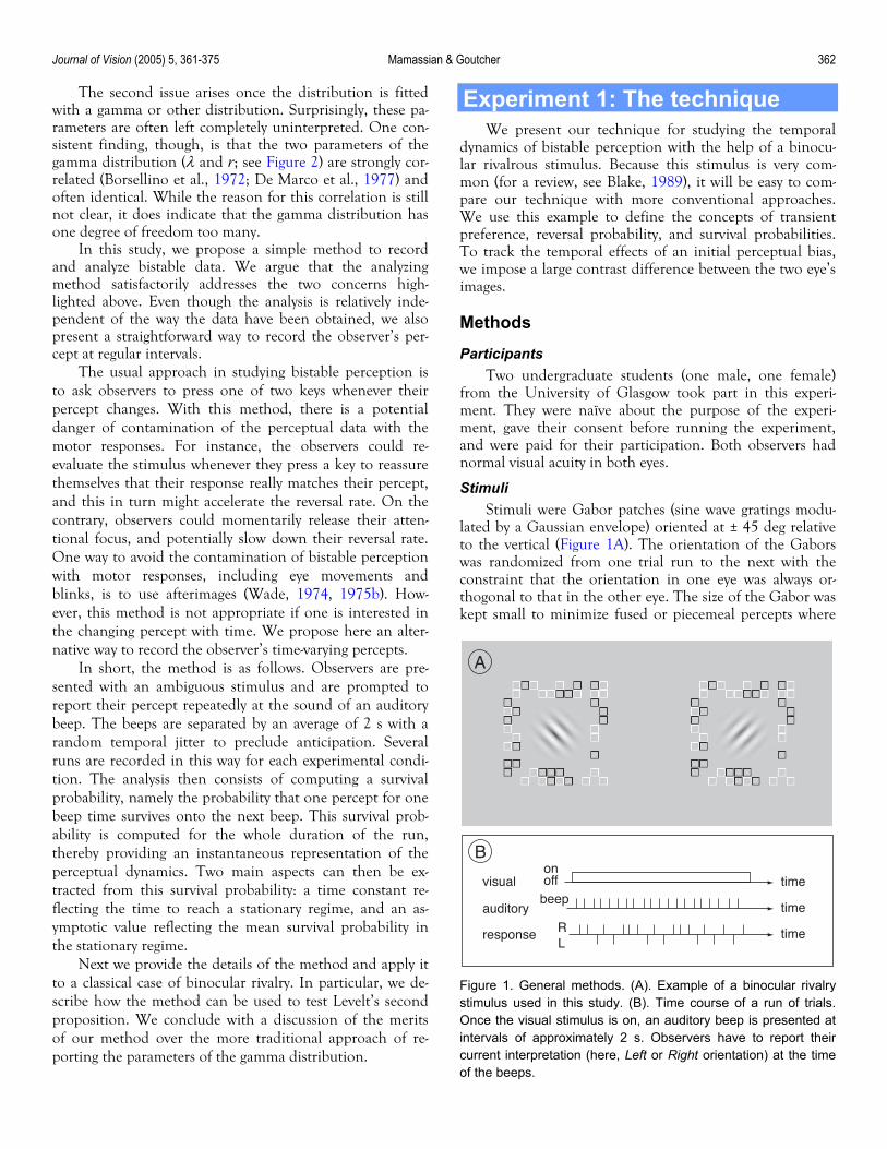
lated by a Gaussian envelope) oriented at ± 45 deg relative to the vertical (Figure 1A). The orientation of the Gabors was randomized from one trial run to the next with the constraint that the orientation in one eye was always or-thogonal to that in the other eye. The size of the Gabor was kept small to minimize fused or piecemeal percepts where

FsOico

timevisual

auditory

response

time

time

onoff

beep

RL

B

A

igure 1. General methods. (A). Example of a binocular rivalrytimulus used in this study. (B). Time course of a run of trials.nce the visual stimulus is on, an auditory beep is presented at

ntervals of approximately 2 s. Observers have to report theirurrent interpretation (here, Left or Right orientation) at the timef the beeps.

Journal of Vision (2005) 5, 361-375 Mamassian & Goutcher 363

the interpretation is a mixture of the left and right images. The size (at half-height of the Gaussian envelope) was 0.83 deg of visual angle in diameter. The spatial frequency of the grating was set to 2.5 cycles/deg. The contrast ratio between the left and right eye images was fixed to 25%. Which eye saw the full-contrast Gabor and which eye saw the 25%-contrast Gabor was randomized between trials. In the analyses below, we combine trials according to the stimulus contrast, so we present our results relative to ei-ther the high-contrast or low-contrast stimulus rather than left or right eye.

The stimuli were surrounded by a frame composed of small squares, half of them black, the others white. This frame was non-rivalrous (same contrast in both eyes) and had zero disparity.

Stimuli were presented on a split-screen Wheatstone stereoscope where the display was a 21-in Sony Trinitron CRT monitor driven by an Apple PowerMac computer. The experiment was controlled by a program that ran un-der Matlab using the PsychToolbox functions (Brainard, 1997; Pelli, 1997). The experiment was run in a dark room and the observers had to place their heads in a chin- and head-rest to minimize head movements. The viewing dis-tance was 80 cm.

Procedure Observers were repeatedly prompted to report the per-

ceived orientation of the Gabor at the sound of an auditory beep (Figure 1B). Beeps were presented on average every 2 s, starting 1 s after the stimulus onset. A small temporal jitter was introduced to reduce anticipatory responses. This jitter was drawn from a uniform distribution extending 500 ms before and after the planned mean time occurrence of the beeps. In practice, the first beep could therefore oc-cur anytime between 0.5 s and 1.5 s after stimulus onset, the next beep anytime between 2.5 s and 3.5 s, and so on.

Observers had to press one of two keys with their left or right index fingers, reporting their percept at the time of the beep. If uncertain, they were asked to choose the per-cept that appeared the strongest. Responses made more than 1 s after the beep were discarded. This strict constraint allowed us to ascertain that a response did not interact with the next beep. To minimize the probability of missing the first beep, a count-down from 5 s before the stimulus onset was displayed on the monitor. The zero-disparity frame was also presented during this count-down to help stabilize ver-gence before stimulus onset.

In this first experiment, the presentation duration of a run (the time when the Gabors were shown) was set to 50 s. Each observer ran 100 such runs (50 at each contrast ratio balanced across the two eyes) with a short break between consecutive runs.

Results The results are split in phase durations, transient pref-

erence, reversal probability, and survival probabilities.

Phase durations The traditional way to analyze data from bistable ex-

periments is to report the distribution of the phase dura-tions. Phase durations of each dominant percept (here the orientation of the high- and low-contrast Gabors) can be computed by counting the consecutive number of times that a given percept is reported to be identical. For in-stance, if the same orientation is perceived for three con-secutive beeps before the percept reverses to the other ori-entation, this particular phase will be assigned a duration of 6 s (3 times the inter-beep interval of 2 s).

It is clear that the phase durations we have recorded are affected by the inter-beep interval. We missed phase durations shorter than 2 s, but also slightly exaggerated all phase durations (by combining two phases that were sepa-rated by a missed phase). More discussions of this issue can be found in Appendix D.

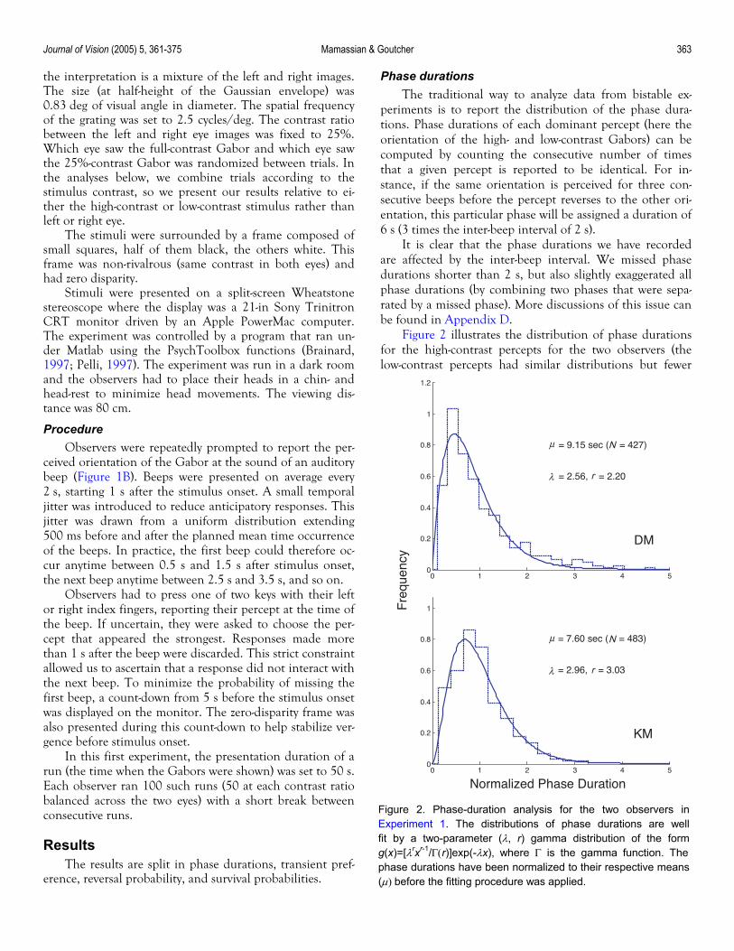
Figure 2 illustrates the distribution of phase durations for the high-contrast percepts for the two observers (the low-contrast percepts had similar distributions but fewer

0 1 2 3 4 50

0.2

0.4

0.6

0.8

1

1.2

= 9.15 sec ( = 427)

= 2.56, = 2.20

DM

0 1 2 3 4 50

0.2

0.4

0.6

0.8

1

= 7.60 sec ( = 483)

= 2.96, = 3.03

Normalized Phase Duration

Fre

quen

cy

KM

N

r

µ

λ

N

r

µ

λ

Figure 2. Phase-duration analysis for the two observers inExperiment 1. The distributions of phase durations are wellfit by a two-parameter (λ, r) gamma distribution of the formg(x)=[λrxr-1/Γ(r)]exp(-λx), where Γ is the gamma function. Thephase durations have been normalized to their respective means(µ) before the fitting procedure was applied.

Journal of Vision (2005) 5, 361-375 Mamassian & Goutcher 364

0 10 20 30 40 500

0.1

0.2

0.3

0.4

0.5

0.6

0.7

0.8

0.9

1

Time (s)

= 0.708

= 7.3 s

= – 0.070 s-1

Tran

sien

t Pre

fere

nce

KM

0

0.1

0.2

0.3

0.4

0.5

0.6

0.7

0.8

0.9

1

= 0.709

= 21.5 s

= – 0.018 s-1DM

α

τ

σ

α

τ

σ

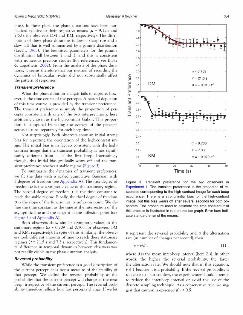
bins). In these plots, the phase durations have been nor-malized relative to their respective means (µ = 9.15 s and 7.60 s for observers DM and KM, respectively). The distri-bution of these phase durations follows a sharp rise and a slow fall that is well summarized by a gamma distribution (Levelt, 1965). The best-fitted parameters for the gamma distribution fall between 2 and 3, and this is consistent with numerous previous studies (for references, see Blake & Logothetis, 2002). From this analysis of the phase dura-tions, it seems therefore that our method of recording the dynamics of binocular rivalry did not substantially affect the pattern of responses.

Transient preference What the phase-duration analysis fails to capture, how-

ever, is the time course of the percepts. A natural depiction of this time course is provided by the transient preference. The transient preference is simply the proportion of per-cepts consistent with one of the two interpretations, here arbitrarily chosen as the high-contrast Gabor. This propor-tion is computed by taking the average of the percepts across all runs, separately for each beep time.

Not surprisingly, both observers show an initial strong bias for reporting the orientation of the high-contrast im-age. The initial bias is in fact so consistent with the high-contrast image that the transient probability is not signifi-cantly different from 1 at the first beep. Interestingly though, this initial bias gradually wears off and the tran-sient preference reaches a stable regime (Figure 3).

To summarize the dynamics of transient preferences, we fit the data with a scaled cumulative Gaussian with 3 degrees of freedom (see Appendix A). The first degree of freedom α is the asymptotic value of the stationary regime. The second degree of freedom τ is the time constant to reach the stable regime. Finally, the third degree of freedom σ is the slope of the function at its inflexion point. We de-fine the time constant as the time at the intersection of the asymptotic line and the tangent at the inflexion point (see Figure 3 and Appendix A).

Figure 3. Transient preference for the two observers inExperiment 1. The transient preference is the proportion of re-sponses corresponding to the high-contrast image for each beepoccurrence. There is a strong initial bias for the high-contrastimage, but this bias wears off after several seconds for both ob-servers. The procedure used to estimate the time constant τ ofthis process is illustrated in red on the top graph. Error bars indi-cate standard error of the means.

Both observers show similar asymptotic values in the stationary regime (α = 0.709 and 0.708 for observers DM and KM, respectively). In spite of this similarity, the observ-ers took different amounts of time to reach these stationary regimes (τ = 21.5 s and 7.3 s, respectively). This fundamen-tal difference in temporal dynamics between observers was not readily visible in the phase-duration analysis.

Reversal probability While the transient preference is a good description of

the current percept, it is not a measure of the stability of that percept. We define the reversal probability as the probability that the current percept will change at the next beep, irrespective of the current percept. The reversal prob-ability therefore reflects how fast percepts change. If we let

v represent the reversal probability and u the alternation rate (in number of changes per second), then

u v δ= , (1)

where δ is the mean inter-beep interval (here 2 s). In other words, the higher the reversal probability, the faster the alternation rate. We should note that in this equation, v ≤ 1 because it is a probability. If the reversal probability is too close to 1 for comfort, the experimenter should attempt to reduce the inter-beep interval or avoid the use of the discrete sampling technique. As a conservative rule, we sug-gest that caution is exercised if v > 0.5.

Journal of Vision (2005) 5, 361-375 Mamassian & Goutcher 365

0 10 20 30 40 500

0.1

0.2

0.3

0.4

0.5

0.6

0.7

0.8

0.9

1

Time (s)

= 0.366

= 5.29 s

= 0.108 s-1

KM

0

0.1

0.2

0.3

0.4

0.5

0.6

0.7

0.8

0.9

1

= 0.373

= 19.47 s

= 0.023 s-1

Rev

ersa

l Pro

babi

lity

DM

α

τ

σ

α

τ

σ

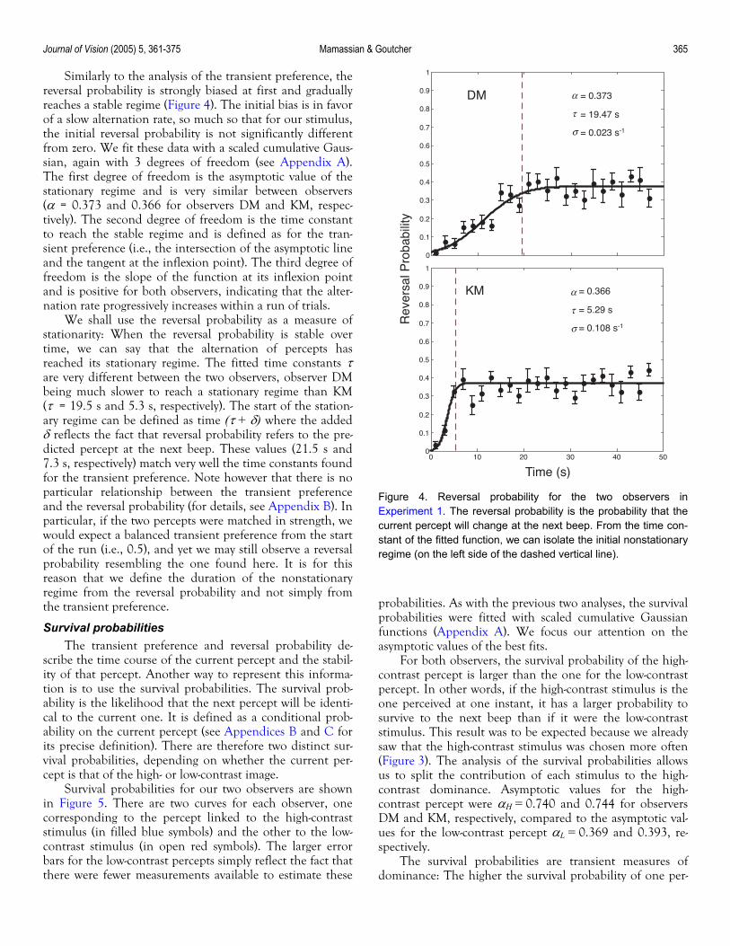
Similarly to the analysis of the transient preference, the reversal probability is strongly biased at first and gradually reaches a stable regime (Figure 4). The initial bias is in favor of a slow alternation rate, so much so that for our stimulus, the initial reversal probability is not significantly different from zero. We fit these data with a scaled cumulative Gaus-sian, again with 3 degrees of freedom (see Appendix A). The first degree of freedom is the asymptotic value of the stationary regime and is very similar between observers (α = 0.373 and 0.366 for observers DM and KM, respec-tively). The second degree of freedom is the time constant to reach the stable regime and is defined as for the tran-sient preference (i.e., the intersection of the asymptotic line and the tangent at the inflexion point). The third degree of freedom is the slope of the function at its inflexion point and is positive for both observers, indicating that the alter-nation rate progressively increases within a run of trials.

We shall use the reversal probability as a measure of stationarity: When the reversal probability is stable over time, we can say that the alternation of percepts has reached its stationary regime. The fitted time constants τ are very different between the two observers, observer DM being much slower to reach a stationary regime than KM (τ = 19.5 s and 5.3 s, respectively). The start of the station-ary regime can be defined as time (τ + δ) where the added δ reflects the fact that reversal probability refers to the pre-dicted percept at the next beep. These values (21.5 s and 7.3 s, respectively) match very well the time constants found for the transient preference. Note however that there is no particular relationship between the transient preference and the reversal probability (for details, see Appendix B). In particular, if the two percepts were matched in strength, we would expect a balanced transient preference from the start of the run (i.e., 0.5), and yet we may still observe a reversal probability resembling the one found here. It is for this reason that we define the duration of the nonstationary regime from the reversal probability and not simply from the transient preference.

Figure 4. Reversal probability for the two observers inExperiment 1. The reversal probability is the probability that thecurrent percept will change at the next beep. From the time con-stant of the fitted function, we can isolate the initial nonstationaryregime (on the left side of the dashed vertical line).

Survival probabilities The transient preference and reversal probability de-

scribe the time course of the current percept and the stabil-ity of that percept. Another way to represent this informa-tion is to use the survival probabilities. The survival prob-ability is the likelihood that the next percept will be identi-cal to the current one. It is defined as a conditional prob-ability on the current percept (see Appendices B and C for its precise definition). There are therefore two distinct sur-vival probabilities, depending on whether the current per-cept is that of the high- or low-contrast image.

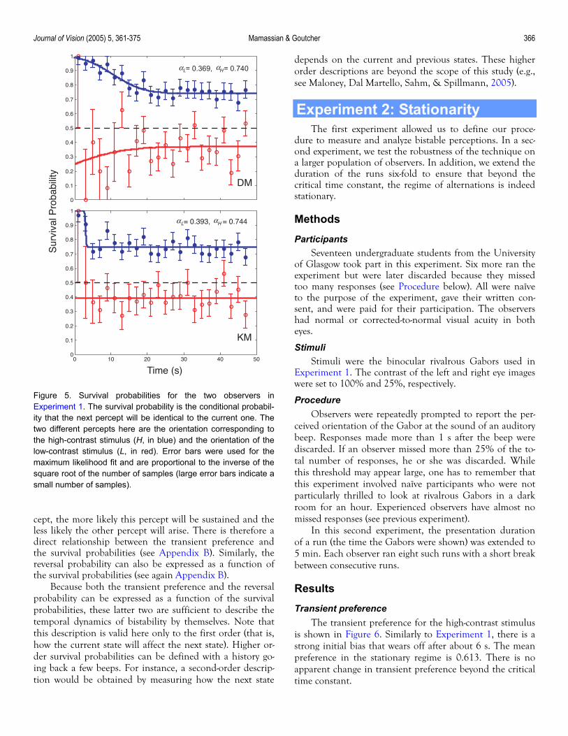
Survival probabilities for our two observers are shown in Figure 5. There are two curves for each observer, one corresponding to the percept linked to the high-contrast stimulus (in filled blue symbols) and the other to the low-contrast stimulus (in open red symbols). The larger error bars for the low-contrast percepts simply reflect the fact that there were fewer measurements available to estimate these

probabilities. As with the previous two analyses, the survival probabilities were fitted with scaled cumulative Gaussian functions (Appendix A). We focus our attention on the asymptotic values of the best fits.

For both observers, the survival probability of the high-contrast percept is larger than the one for the low-contrast percept. In other words, if the high-contrast stimulus is the one perceived at one instant, it has a larger probability to survive to the next beep than if it were the low-contrast stimulus. This result was to be expected because we already saw that the high-contrast stimulus was chosen more often (Figure 3). The analysis of the survival probabilities allows us to split the contribution of each stimulus to the high-contrast dominance. Asymptotic values for the high-contrast percept were αH = 0.740 and 0.744 for observers DM and KM, respectively, compared to the asymptotic val-ues for the low-contrast percept αL = 0.369 and 0.393, re-spectively.

The survival probabilities are transient measures of dominance: The higher the survival probability of one per-

Journal of Vision (2005) 5, 361-375 Mamassian & Goutcher 366

cept, the more likely this percept will be sustained and the less likely the other percept will arise. There is therefore a direct relationship between the transient preference and the survival probabilities (see Appendix B). Similarly, the reversal probability can also be expressed as a function of the survival probabilities (see again Appendix B).

Because both the transient preference and the reversal probability can be expressed as a function of the survival probabilities, these latter two are sufficient to describe the temporal dynamics of bistability by themselves. Note that this description is valid here only to the first order (that is, how the current state will affect the next state). Higher or-der survival probabilities can be defined with a history go-ing back a few beeps. For instance, a second-order descrip-tion would be obtained by measuring how the next state

depends on the current and previous states. These higher order descriptions are beyond the scope of this study (e.g., see Maloney, Dal Martello, Sahm, & Spillmann, 2005).

0 10 20 30 40 500

0.1

0.2

0.3

0.4

0.5

0.6

0.7

0.8

0.9

1

Time (s)

= 0.393, = 0.744

Sur

viva

l Pro

babi

lity

KM

0

0.1

0.2

0.3

0.4

0.5

0.6

0.7

0.8

0.9

1

= 0.369, = 0.740

DM

α αL H

α αL H

Experiment 2: Stationarity The first experiment allowed us to define our proce-

dure to measure and analyze bistable perceptions. In a sec-ond experiment, we test the robustness of the technique on a larger population of observers. In addition, we extend the duration of the runs six-fold to ensure that beyond the critical time constant, the regime of alternations is indeed stationary.

Methods

Participants Seventeen undergraduate students from the University

of Glasgow took part in this experiment. Six more ran the experiment but were later discarded because they missed too many responses (see Procedure below). All were naïve to the purpose of the experiment, gave their written con-sent, and were paid for their participation. The observers had normal or corrected-to-normal visual acuity in both eyes.

Stimuli Stimuli were the binocular rivalrous Gabors used in

Experiment 1. The contrast of the left and right eye images were set to 100% and 25%, respectively.

Figure 5. Survival probabilities for the two observers inExperiment 1. The survival probability is the conditional probabil-ity that the next percept will be identical to the current one. Thetwo different percepts here are the orientation corresponding tothe high-contrast stimulus (H, in blue) and the orientation of thelow-contrast stimulus (L, in red). Error bars were used for themaximum likelihood fit and are proportional to the inverse of thesquare root of the number of samples (large error bars indicate asmall number of samples).

Procedure Observers were repeatedly prompted to report the per-

ceived orientation of the Gabor at the sound of an auditory beep. Responses made more than 1 s after the beep were discarded. If an observer missed more than 25% of the to-tal number of responses, he or she was discarded. While this threshold may appear large, one has to remember that this experiment involved naïve participants who were not particularly thrilled to look at rivalrous Gabors in a dark room for an hour. Experienced observers have almost no missed responses (see previous experiment).

In this second experiment, the presentation duration of a run (the time the Gabors were shown) was extended to 5 min. Each observer ran eight such runs with a short break between consecutive runs.

Results

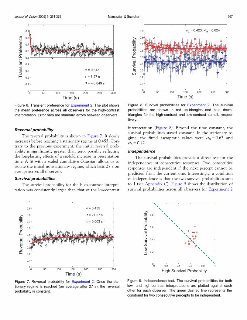
Transient preference The transient preference for the high-contrast stimulus

is shown in Figure 6. Similarly to Experiment 1, there is a strong initial bias that wears off after about 6 s. The mean preference in the stationary regime is 0.613. There is no apparent change in transient preference beyond the critical time constant.

Journal of Vision (2005) 5, 361-375 Mamassian & Goutcher 367

0 50 100 150 200 250 3000

0.1

0.2

0.3

0.4

0.5

0.6

0.7

0.8

0.9

1

Time (s)

Tra

nsie

nt P

refe

renc

e

= 0.613

= 6.27 s

= – 0.049 s-1

α

τ

σ

Figure 6. Transient preference for Experiment 2. The plot showsthe mean preference across all observers for the high-contrastinterpretation. Error bars are standard errors between observers.

Reversal probability The reversal probability is shown in Figure 7. It slowly

increases before reaching a stationary regime at 0.455. Con-trary to the previous experiment, the initial reversal prob-ability is significantly greater than zero, possibly reflecting the long-lasting effects of a six-fold increase in presentation time. A fit with a scaled cumulative Gaussian allows us to isolate the initial nonstationary regime, which lasts 27 s on average across all observers.

Survival probabilities The survival probability for the high-contrast interpre-

tation was consistently larger than that of the low-contrast

interpretation (Figure 8). Beyond the time constant, the survival probabilities stayed constant. In the stationary re-gime, the fitted asymptotic values were αH = 0.62 and αL = 0.42.

Independence The survival probabilities provide a direct test for the

independence of consecutive responses. Two consecutive responses are independent if the next percept cannot be predicted from the current one. Interestingly, a condition of independence is that the two survival probabilities sum to 1 (see Appendix C). Figure 9 shows the distribution of survival probabilities across all observers for Experiment 2

0 50 100 150 200 250 3000

0.1

0.2

0.3

0.4

0.5

0.6

0.7

0.8

0.9

1

Time (s)

Sur

viva

l Pro

babi

lity

= 0.423, = 0.624α αL H

0 0.2 0.4 0.6 0.8 10

0.2

0.4

0.6

0.8

1

High Survival Probability

Low

Sur

viva

l Pro

babi

lity

Figure 9. Independence test. The survival probabilities for bothlow- and high-contrast interpretations are plotted against eachother for each observer. The green dashed line represents theconstraint for two consecutive percepts to be independent.

Figure 8. Survival probabilities for Experiment 2. The survivalprobabilities are shown in red up-triangles and blue down-triangles for the high-contrast and low-contrast stimuli, respec-tively.

0 50 100 150 200 250 3000

0.1

0.2

0.3

0.4

0.5

0.6

0.7

0.8

0.9

1

Time (s)

Rev

ersa

l Pro

babi

lity

= 0.455

= 27.27 s

= 0.003 s-1

α

τ

σ

Figure 7. Reversal probability for Experiment 2. Once the sta-tionary regime is reached (on average after 27 s), the reversalprobability is constant.

Journal of Vision (2005) 5, 361-375 Mamassian & Goutcher 368

(once they have reached the stationary regime). The sums of the pairs of survival probabilities for each observer are on average larger than 1 (mean: 1.050; SE across observers: 0.029), indicating that consecutive percepts are not inde-pendent. This result is seemingly in contradiction with pre-vious reports that have consistently argued for independ-ence (Fox & Hermann, 1967; Blake, Fox, & McIntyre, 1971; Walker, 1975; Lehky, 1995). However, it is impor-tant to remember that their independence test was on con-secutive phase durations rather than consecutive percepts. Our dependence result might reflect the gradual build-up of adaptation to one percept while this percept is surviving, whereas the independence of phase durations suggests that the adaptation is reset whenever a transition occurs.

Experiment 3: Perceptual biases The first two experiments have demonstrated the use of

the survival probabilities to describe the temporal dynamics of bistable perception. In this third experiment, we look at how the survival probabilities vary with the strength of the competing stimuli. We vary the relative strength of each stimulus by altering the contrast of the stimulus in one or the other eye.

Methods

Participants Twenty-two naive undergraduate students took part in

this experiment. Seven of these participants were discarded because they failed to respond quickly enough (see Proce-dure below). The analysis below was carried out on the 15 remaining participants.

Stimuli Stimuli were identical to those used in the previous ex-

periment, except that six contrast conditions were used. The contrast ratios between the right and left eyes were chosen equi-distant on a log-scale: 0.5, 0.66, 0.87, 1.15, 1.52, or 2.0. The first three contrasts were obtained by set-ting the contrast of the left eye to 1.0 and varying the con-trast of the right eye between 0.5 and 0.87 (see legend of Figure 13); the last three contrasts were similarly obtained by exchanging the roles of the left and right eyes.

Procedure The procedure was similar to that used in the previous

experiment. Observers ran eight consecutive blocks of runs where each block contained one run for each contrast ratio, presented in random order. Observers took a short break between each run and a longer break between each block.

The inter-beep interval was again 2 s on average and participants had to respond within 1 s after each beep. Those participants who missed more than 25% of the re-sponses were removed from the final analysis.

Results

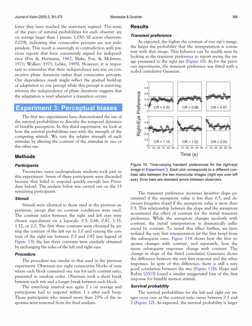
Transient preference As expected, the higher the contrast of one eye’s image,

the larger the probability that the interpretation is consis-tent with that image. This behavior can be readily seen by looking at the transient preference to report seeing the im-age presented to the right eye (Figure 10). As for the previ-ous experiments, the transient preference was fitted with a scaled cumulative Gaussian.

0

0.2

0.4

0.6

0.8

1

CR = 0.50 CR = 0.66 CR = 0.87

0 10 20 30 40 500

0.2

0.4

0.6

0.8

1

CR = 1.15

0 10 20 30 40 50

CR = 1.52

0 10 20 30 40 50

CR = 2.00

Time (s)

Rig

ht-E

ye P

refe

renc

e

Figure 10. Time-varying transient preferences for the right-eyeimage in Experiment 3. Each plot corresponds to a different con-trast ratio between the two monocular images (right eye over lefteye). Error bars are standard errors between observers.

The transient preference increases (positive slope pa-

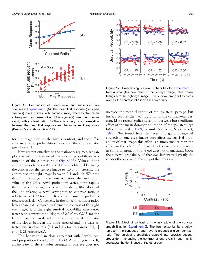
rameter) if the asymptotic value is less than 0.5, and de-creases (negative slope) if the asymptotic value is more than 0.5. This relationship between the slope and the asymptote accentuates the effect of contrast for the initial transient preference. While the asymptote changes modestly with contrast, the initial interpretation is dramatically influ-enced by contrast. To reveal this effect further, we have isolated the very first interpretation (at the first beep) from the subsequent ones. Figure 11A shows how the first re-sponse changes with contrast, and separately, how the mean subsequent responses change with contrast. The change in slope of the fitted cumulative Gaussians shows the difference between the very first response and the other responses. In spite of this difference, there is still a very good correlation between the two (Figure 11B). Hupé and Rubin (2003) found a similar exaggerated bias of the first response for bistable motion stimuli.

Survival probability The survival probabilities for the left and right eye im-

ages cross over as the contrast ratio varies between 0.5 and 2 (Figure 12). As expected, the survival probability is larger

Journal of Vision (2005) 5, 361-375 Mamassian & Goutcher 369

0

0.2

0.4

0.6

0.8

1

CR = 0.50 CR = 0.66 CR = 0.87

0 10 20 30 40 500

0.2

0.4

0.6

0.8

1

CR = 1.150 10 20 30 40 50

Time (s)

CR = 1.520 10 20 30 40 50

CR = 2.00

Sur

viva

l Pro

babi

lity

Mea

n R

espo

nse

(A)

0 0.5 10.3

0.4

0.5

0.6

0.7

Mean First Response

= 0.79

Mea

n S

ubse

quen

tR

espo

nses

(B)

0.5 1 20

0.2

0.4

0.6

0.8

1

Contrast Ratio

R

Figure 12. Time-varying survival probabilities for Experiment 3.Red up-triangles now refer to the left-eye image, blue down-triangles to the right-eye image. The survival probabilities crossover as the contrast ratio increases over unity.

for the image that has the higher contrast, and the differ-ence in survival probabilities reduces as the contrast ratio gets close to 1.

If we restrict ourselves to the stationary regimes, we can plot the asymptotic value of the survival probabilities as a function of the contrast ratio (Figure 13). Values of the contrast ratio between 0.5 and 1.0 were obtained by fixing the contrast of the left eye image to 1.0 and increasing the contrast of the right image between 0.5 and 1.0. We note that in this range of the contrast ratios, the asymptotic value of the left survival probability varies more rapidly than that of the right survival probability (the slope of the line relating survival asymptote to contrast ratio is –0.246 vs. –0.079 for the left and right survival probabili-ties, respectively). Conversely, in the range of contrast ratios larger than 1.0, obtained by fixing the contrast of the right eye image, it is the right survival probability that varies faster with contrast ratio (slopes of 0.040 vs. 0.213 for the left and right survival probabilities, respectively). The ratio of the slopes between the most affected and the least af-fected eyes is close to 4 (3.1 and 5.3 for the ranges [0.5, 1] and [1, 2], respectively).

This behavior is in close agreement with Levelt’s sec-ond proposition (Levelt, 1965, 1966). According to Levelt, an increase of the stimulus strength in one eye does not

increase the mean duration of the ipsilateral percept, but instead reduces the mean duration of the contralateral per-cept. More recent studies have found a weak but significant effect of the mean dominant duration of the ipsilateral eye (Mueller & Blake, 1989; Bossink, Stalmeier, & de Weert, 1993). We found here that even though a change of strength of one eye’s image does affect the survival prob-ability of that image, this effect is 4 times smaller than the effect on the other eye’s image. In other words, an increase in stimulus strength in one eye does not dramatically boost the survival probability of that eye, but instead greatly de-creases the survival probability of the other eye.

Figure 11. Comparison of mean initial and subsequent re-sponses in Experiment 3. (A). The mean first response (red opensymbols) rises quickly with contrast ratio, whereas the meansubsequent responses (filled blue symbols) rise much moreslowly with contrast ratio. (B).There is a very good correlationbetween the mean first response and the subsequent responses(Pearson’s correlation, R = 0.79).

0.5 1 20

0.2

0.4

0.6

0.8

1

Contrast Ratio

Sur

viva

lA

sym

ptot

e LE RE

1.0LE 1.0

1.00.5RE 1.0

0.5

Figure 13. Effect of contrast on the asymptote of the survivalprobabilities for Experiment 3. The two horizontal bars belowrepresent the contrast of each eye to produce a given contrastratio. The survival probabilities approximate Levelt’s secondproposition: Increasing the contrast of one eye’s image mainlydecreases the dominance of the other eye.

Journal of Vision (2005) 5, 361-375 Mamassian & Goutcher 370

0 0.2 0.4 0.6 0.8 10

0.2

0.4

0.6

0.8

1

LE Survival Prob.

RE

Sur

viva

l Pro

b.

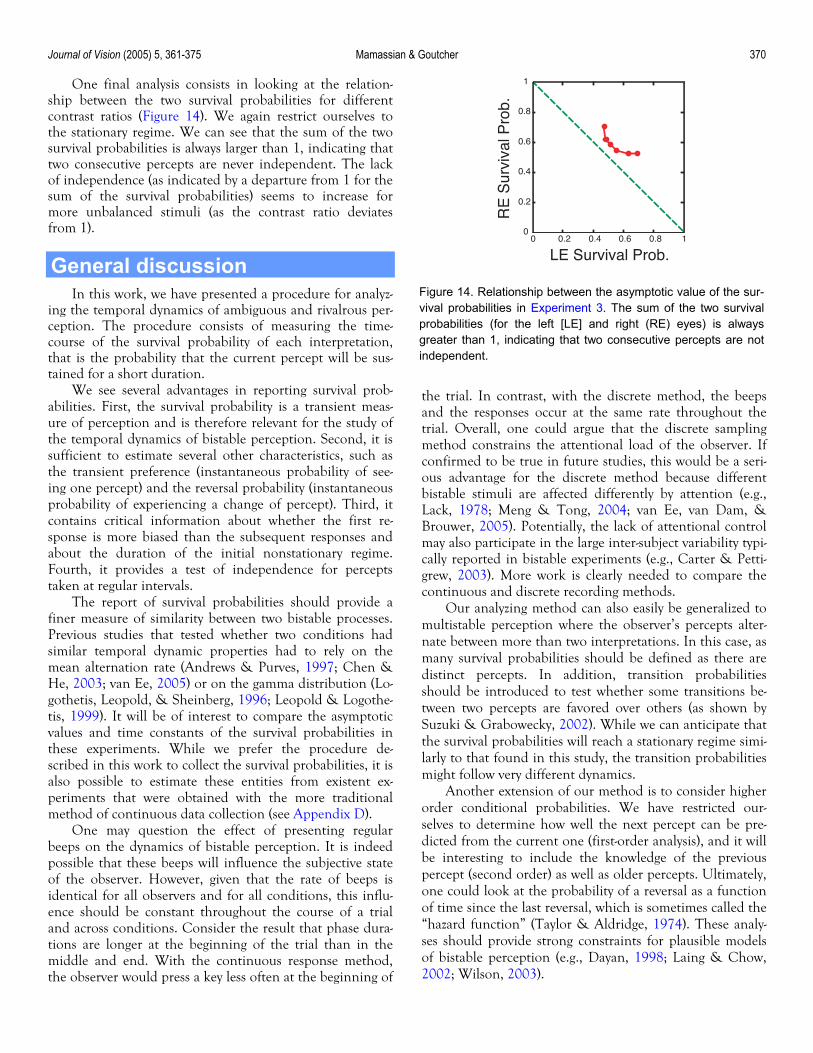
One final analysis consists in looking at the relation-ship between the two survival probabilities for different contrast ratios (Figure 14). We again restrict ourselves to the stationary regime. We can see that the sum of the two survival probabilities is always larger than 1, indicating that two consecutive percepts are never independent. The lack of independence (as indicated by a departure from 1 for the sum of the survival probabilities) seems to increase for more unbalanced stimuli (as the contrast ratio deviates from 1).

General discussion

Figure 14. Relationship between the asymptotic value of the sur-vival probabilities in Experiment 3. The sum of the two survivalprobabilities (for the left [LE] and right (RE) eyes) is alwaysgreater than 1, indicating that two consecutive percepts are notindependent.

In this work, we have presented a procedure for analyz-ing the temporal dynamics of ambiguous and rivalrous per-ception. The procedure consists of measuring the time-course of the survival probability of each interpretation, that is the probability that the current percept will be sus-tained for a short duration.

We see several advantages in reporting survival prob-abilities. First, the survival probability is a transient meas-ure of perception and is therefore relevant for the study of the temporal dynamics of bistable perception. Second, it is sufficient to estimate several other characteristics, such as the transient preference (instantaneous probability of see-ing one percept) and the reversal probability (instantaneous probability of experiencing a change of percept). Third, it contains critical information about whether the first re-sponse is more biased than the subsequent responses and about the duration of the initial nonstationary regime. Fourth, it provides a test of independence for percepts taken at regular intervals.

The report of survival probabilities should provide a finer measure of similarity between two bistable processes. Previous studies that tested whether two conditions had similar temporal dynamic properties had to rely on the mean alternation rate (Andrews & Purves, 1997; Chen & He, 2003; van Ee, 2005) or on the gamma distribution (Lo-gothetis, Leopold, & Sheinberg, 1996; Leopold & Logothe-tis, 1999). It will be of interest to compare the asymptotic values and time constants of the survival probabilities in these experiments. While we prefer the procedure de-scribed in this work to collect the survival probabilities, it is also possible to estimate these entities from existent ex-periments that were obtained with the more traditional method of continuous data collection (see Appendix D).

One may question the effect of presenting regular beeps on the dynamics of bistable perception. It is indeed possible that these beeps will influence the subjective state of the observer. However, given that the rate of beeps is identical for all observers and for all conditions, this influ-ence should be constant throughout the course of a trial and across conditions. Consider the result that phase dura-tions are longer at the beginning of the trial than in the middle and end. With the continuous response method, the observer would press a key less often at the beginning of

the trial. In contrast, with the discrete method, the beeps and the responses occur at the same rate throughout the trial. Overall, one could argue that the discrete sampling method constrains the attentional load of the observer. If confirmed to be true in future studies, this would be a seri-ous advantage for the discrete method because different bistable stimuli are affected differently by attention (e.g., Lack, 1978; Meng & Tong, 2004; van Ee, van Dam, & Brouwer, 2005). Potentially, the lack of attentional control may also participate in the large inter-subject variability typi-cally reported in bistable experiments (e.g., Carter & Petti-grew, 2003). More work is clearly needed to compare the continuous and discrete recording methods.

Our analyzing method can also easily be generalized to multistable perception where the observer’s percepts alter-nate between more than two interpretations. In this case, as many survival probabilities should be defined as there are distinct percepts. In addition, transition probabilities should be introduced to test whether some transitions be-tween two percepts are favored over others (as shown by Suzuki & Grabowecky, 2002). While we can anticipate that the survival probabilities will reach a stationary regime simi-larly to that found in this study, the transition probabilities might follow very different dynamics.

Another extension of our method is to consider higher order conditional probabilities. We have restricted our-selves to determine how well the next percept can be pre-dicted from the current one (first-order analysis), and it will be interesting to include the knowledge of the previous percept (second order) as well as older percepts. Ultimately, one could look at the probability of a reversal as a function of time since the last reversal, which is sometimes called the “hazard function” (Taylor & Aldridge, 1974). These analy-ses should provide strong constraints for plausible models of bistable perception (e.g., Dayan, 1998; Laing & Chow, 2002; Wilson, 2003).

Journal of Vision (2005) 5, 361-375 Mamassian & Goutcher 371

In summary, we have proposed a technique to measure and analyze some of the fundamental properties of the temporal dynamics of ambiguous and rivalrous perception. We are currently measuring the survival probabilities in a variety of bistable stimuli to compare the similarities across stimuli and tasks.

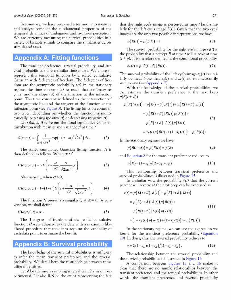
Appendix A: Fitting functions The transient preference, reversal probability, and sur-

vival probabilities share a similar time-course. We chose to represent this temporal function by a scaled cumulative Gaussian with 3 degrees of freedom. The 3 degrees of free-dom are the asymptotic probability (α) in the stationary regime, the time constant (τ) to reach that stationary re-gime, and the slope (σ) of the function at the inflection point. The time constant is defined as the intersection of the asymptotic line and the tangent of the function at the inflexion point (see Figure 3). The fitting function comes in two types, depending on whether the function is mono-tonically increasing (positive σ) or decreasing (negative σ).

Let G(m, s, t) represent the usual cumulative Gaussian distribution with mean m and variance s2 at time t

( )( )2 22

1( , , ) exp 22

tG m s t x m s dx

sπ−∞

= − −∫ . (2)

The scaled cumulative Gaussian fitting function H is then defined as follows. When σ > 0,

2( , , , ) , ,

2 2H t G tα αα τ σ α τ

σ πσ

= −

. (3) p R

Alternatively, when σ < 0,

( )2

1 1( , , , ) 1 1 , ,2 2

H t G α αα τ σ α τσ πσ

− − = − − +

t

. (4)

The function H presents a singularity at σ = 0. By con-vention, we shall define

( , ,0, )H tα τ = α . (5) p R

The 3 degrees of freedom of the scaled cumulative function H were adjusted to the data with a maximum like-lihood procedure that took into account the variability of each data point to estimate the best fit.

Appendix B: Survival probability The knowledge of the survival probabilities is sufficient

to infer the mean transient preference and the reversal probability. We detail here the relationships between these different entities.

Let δ be the mean sampling interval (i.e., 2 s in our ex-periments). Let also R(t) be the event representing the fact

that the right eye’s image is perceived at time t [and simi-larly for the left eye’s image L(t)]. Given that the two eyes’ images are the only two possible interpretations, we have

( ) ( )( ) ( ) 1p R t p L t+ = . (6)

The survival probability for the right eye’s image sR(t) is the probability that a percept R at time t will survive at time (t + δ). It is therefore defined as the conditional probability

( )( ) ( ) | ( )Rs t p R t R tδ= + . (7)

The survival probability of the left eye’s image sL(t) is simi-larly defined. Note that sR(t) and sL(t) do not necessarily sum to one (see Appendix C).

With the knowledge of the survival probabilities, we can estimate the transient preference at the next beep p(R(t + δ))

( )( ) ( ) ( )( ) ( ) ( )( )( )( ) ( )

( )( ) ( )

( ) ( ) ( )( )

, ,

| ( ) ( )

| ( ) ( )

( ) ( ) 1 ( ) 1 ( ) .R L

p R t p R t R t p R t L t

p R t R t p R t

p R t L t p L t

s t p R t s t p R t

δ δ δ

δ

δ

+ = + + +

= + +

+

= + − −

(8)

In the stationary regime, we have

( ) ( )( ) ( ) (p R t p R t p Rδ+ = = ) (9)

and Equation 8 for the transient preference reduces to

( ) ( ) ( )1 2L L Rs s s= − − − . (10)

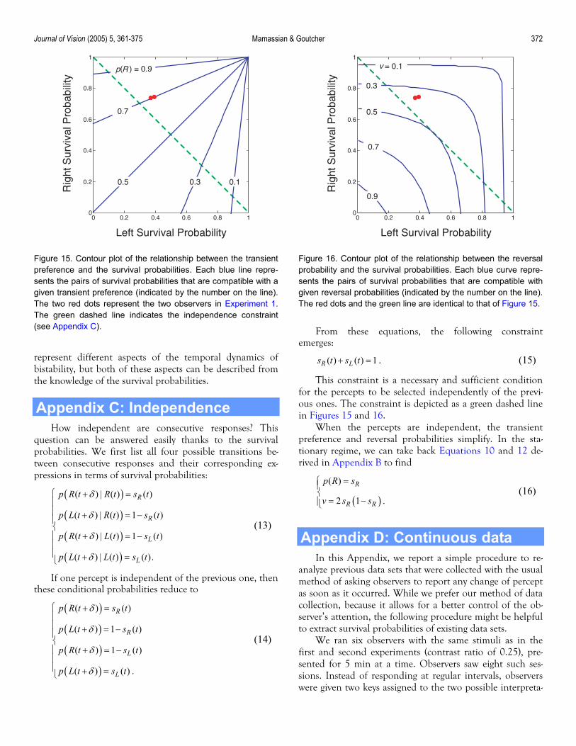
This relationship between transient preference and survival probabilities is illustrated in Figure 15.

In a similar way, the probability v(t) that the current percept will reverse at the next beep can be expressed as

( ) ( )( ) ( ) ( )( )( )( ) ( )

( )( ) ( )

( ) ( ) ( ) ( )( )

( ) , ,

| ( ) ( )

| ( ) ( )

1 ( ) ( ) 1 ( ) 1 ( )R L

v t p L t R t p R t L t

p L t R t p R t

t L t p L t

s t p R t s t p R t

δ δ

δ

δ

= + + +

= + +

+

= − + − −

(11)

.

In the stationary regime, we can use the expression we found for the transient preference probability (Equation 10). In doing this, the reversal probability reduces to

( ) ( ) ( )2 1 1 2L R Lv s s s s= − − − − R . (12)

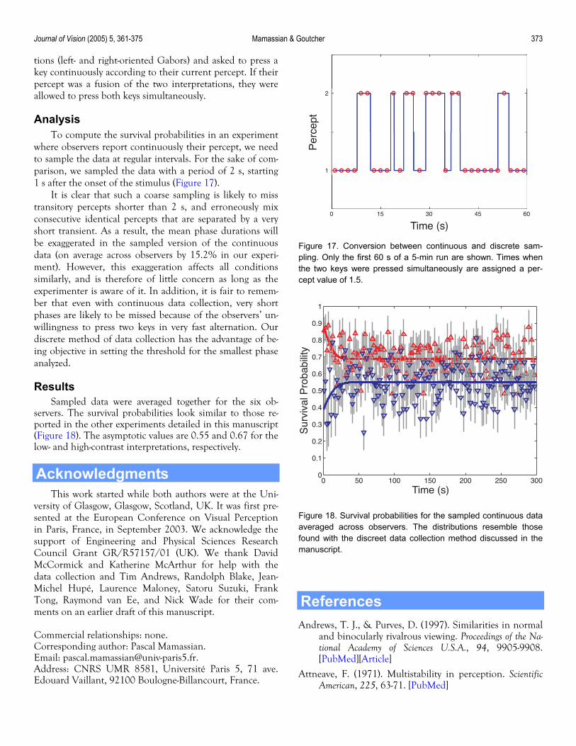
The relationship between the reversal probability and the survival probabilities is illustrated in Figure 16.

A comparison between Figures 15 and 16 makes it clear that there are no simple relationships between the transient preference and the reversal probabilities. In other words, the transient preference and reversal probability

Journal of Vision (2005) 5, 361-375 Mamassian & Goutcher 372

0 0.2 0.4 0.6 0.8 10

0.2

0.4

0.6

0.8

1

Left Survival Probability

Rig

ht S

urvi

val P

roba

bilit

y ( ) = 0.9

0.7

0.5 0.3 0.1

p R

0 0.2 0.4 0.6 0.8 10

0.2

0.4

0.6

0.8

1

Left Survival Probability

Rig

ht S

urvi

val P

roba

bilit

y

= 0.1

0.3

0.5

0.7

0.9

v

Figure 15. Contour plot of the relationship between the transientpreference and the survival probabilities. Each blue line repre-sents the pairs of survival probabilities that are compatible with agiven transient preference (indicated by the number on the line).The two red dots represent the two observers in Experiment 1.The green dashed line indicates the independence constraint(see Appendix C).

Figure 16. Contour plot of the relationship between the reversalprobability and the survival probabilities. Each blue curve repre-sents the pairs of survival probabilities that are compatible withgiven reversal probabilities (indicated by the number on the line).The red dots and the green line are identical to that of Figure 15.

represent different aspects of the temporal dynamics of bistability, but both of these aspects can be described from the knowledge of the survival probabilities.

Appendix C: Independence How independent are consecutive responses? This

question can be answered easily thanks to the survival probabilities. We first list all four possible transitions be-tween consecutive responses and their corresponding ex-pressions in terms of survival probabilities:

( )

( )

( )

( )

( ) | ( ) ( )

( ) | ( ) 1 (

( ) | ( ) 1 (

( ) | ( ) ( ).

R

R

L

L

p R t R t s t

p L t R t s t

p R t L t s t

p L t L t s t

δ

δ

δ

δ

+ = + = −

+ = − + =

)

)

)

)

(13)

If one percept is independent of the previous one, then these conditional probabilities reduce to

( )

( )

( )

( )

( ) ( )

( ) 1 (

( ) 1 (

( ) ( ) .

R

R

L

L

p R t s t

p L t s t

p R t s t

p L t s t

δ

δ

δ

δ

+ = + = −

+ = − + =

(14)

From these equations, the following constraint emerges:

( ) ( ) 1R Ls t s t+ = . (15)

This constraint is a necessary and sufficient condition for the percepts to be selected independently of the previ-ous ones. The constraint is depicted as a green dashed line in Figures 15 and 16.

When the percepts are independent, the transient preference and reversal probabilities simplify. In the sta-tionary regime, we can take back Equations 10 and 12 de-rived in Appendix B to find

( )

( )

2 1

R

R R

p R s

v s s

=

= − . (16)

Appendix D: Continuous data In this Appendix, we report a simple procedure to re-

analyze previous data sets that were collected with the usual method of asking observers to report any change of percept as soon as it occurred. While we prefer our method of data collection, because it allows for a better control of the ob-server’s attention, the following procedure might be helpful to extract survival probabilities of existing data sets.

We ran six observers with the same stimuli as in the first and second experiments (contrast ratio of 0.25), pre-sented for 5 min at a time. Observers saw eight such ses-sions. Instead of responding at regular intervals, observers were given two keys assigned to the two possible interpreta-

Journal of Vision (2005) 5, 361-375 Mamassian & Goutcher 373

0 15 30 45 60

1

2

Time (s)

Per

cept

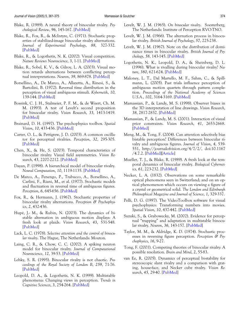
tions (left- and right-oriented Gabors) and asked to press a key continuously according to their current percept. If their percept was a fusion of the two interpretations, they were allowed to press both keys simultaneously.

Analysis To compute the survival probabilities in an experiment

where observers report continuously their percept, we need to sample the data at regular intervals. For the sake of com-parison, we sampled the data with a period of 2 s, starting 1 s after the onset of the stimulus (Figure 17).

It is clear that such a coarse sampling is likely to miss transitory percepts shorter than 2 s, and erroneously mix consecutive identical percepts that are separated by a very short transient. As a result, the mean phase durations will be exaggerated in the sampled version of the continuous data (on average across observers by 15.2% in our experi-ment). However, this exaggeration affects all conditions similarly, and is therefore of little concern as long as the experimenter is aware of it. In addition, it is fair to remem-ber that even with continuous data collection, very short phases are likely to be missed because of the observers’ un-willingness to press two keys in very fast alternation. Our discrete method of data collection has the advantage of be-ing objective in setting the threshold for the smallest phase analyzed.

Figure 17. Conversion between continuous and discrete sam-pling. Only the first 60 s of a 5-min run are shown. Times whenthe two keys were pressed simultaneously are assigned a per-cept value of 1.5.

0 50 100 150 200 250 3000

0.1

0.2

0.3

0.4

0.5

0.6

0.7

0.8

0.9

1

Time (s)

Sur

viva

l Pro

babi

lity

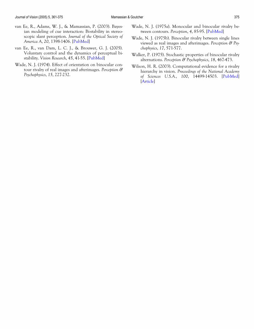
Results Sampled data were averaged together for the six ob-

servers. The survival probabilities look similar to those re-ported in the other experiments detailed in this manuscript (Figure 18). The asymptotic values are 0.55 and 0.67 for the low- and high-contrast interpretations, respectively.

Acknowledgments This work started while both authors were at the Uni-

versity of Glasgow, Glasgow, Scotland, UK. It was first pre-sented at the European Conference on Visual Perception in Paris, France, in September 2003. We acknowledge the support of Engineering and Physical Sciences Research Council Grant GR/R57157/01 (UK). We thank David McCormick and Katherine McArthur for help with the data collection and Tim Andrews, Randolph Blake, Jean-Michel Hupé, Laurence Maloney, Satoru Suzuki, Frank Tong, Raymond van Ee, and Nick Wade for their com-ments on an earlier draft of this manuscript.

Figure 18. Survival probabilities for the sampled continuous dataaveraged across observers. The distributions resemble thosefound with the discreet data collection method discussed in themanuscript.

Commercial relationships: none. Corresponding author: Pascal Mamassian. Email: pascal.mamassian@univ-paris5.fr. Address: CNRS UMR 8581, Université Paris 5, 71 ave. Edouard Vaillant, 92100 Boulogne-Billancourt, France.

References Andrews, T. J., & Purves, D. (1997). Similarities in normal

and binocularly rivalrous viewing. Proceedings of the Na-tional Academy of Sciences U.S.A., 94, 9905-9908. [PubMed][Article]

Attneave, F. (1971). Multistability in perception. Scientific American, 225, 63-71. [PubMed]

Journal of Vision (2005) 5, 361-375 Mamassian & Goutcher 374

Blake, R. (1989). A neural theory of binocular rivalry. Psy-chological Review, 96, 145-167. [PubMed]

Blake, R., Fox, R., & McIntyre, C. (1971). Stochastic prop-erties of stabilized-image binocular rivalry alternations. Journal of Experimental Psychology, 88, 327-332. [PubMed]

Blake, R., & Logothetis, N. K. (2002). Visual competition. Nature Reviews Neuroscience, 3, 1-11. [PubMed]

Blake, R., Sobel, K. V., & Gilroy, L. A. (2003). Visual mo-tion retards alternations between conflicting percep-tual interpretations. Neuron, 39, 869-878. [PubMed]

Borsellino, A., De Marco, A., Allazetta, A., Rinesi, S., & Bartolini, B. (1972). Reversal time distribution in the perception of visual ambiguous stimuli. Kybernetik, 10, 139-144. [PubMed]

Bossink, C. J. H., Stalmeier, P. F. M., & de Weert, Ch. M. M. (1993). A test of Levelt’s second proposition for binocular rivalry. Vision Research, 33, 1413-1419. [PubMed]

Brainard, D. H. (1997). The psychophysics toolbox. Spatial Vision, 10, 433-436. [PubMed]

Carter, O. L., & Pettigrew, J. D. (2003). A common oscilla-tor for perceptual rivalries. Perception, 32, 295-305. [PubMed]

Chen, X., & He, S. (2003). Temporal characteristics of binocular rivalry: Visual field asymmetries. Vision Re-search, 43, 2207-2212. [PubMed]

Dayan, P. (1998). A hierarchical model of binocular rivalry. Neural Computation, 10, 1119-1135. [PubMed]

De Marco, A., Penengo, P., Trabucco, A., Borsellino, A., Carlini, F., Riani, M., et al. (1977). Stochastic models and fluctuation in reversal time of ambiguous figures. Perception, 6, 645-656. [PubMed]

Fox, R., & Hermann, J. (1967). Stochastic properties of binocular rivalry alternations. Perception & Psychophys-ics, 2, 432-436.

Hupé, J.- M., & Rubin, N. (2003). The dynamics of bi-stable alternation in ambiguous motion displays: A fresh look at plaids. Vision Research, 43, 531-548. [PubMed]

Lack, L. C. (1978). Selective attention and the control of binocu-lar rivalry. The Hague, The Netherlands: Mouton.

Laing, C. R., & Chow, C. C. (2002). A spiking neuron model for binocular rivalry. Journal of Computational Neuroscience, 12, 39-53. [PubMed]

Lehky, S. R. (1995). Binocular rivalry is not chaotic. Pro-ceedings of the Royal Society of London B, 259, 71-76. [PubMed]

Leopold, D. A., & Logothetis, N. K. (1999). Multistable phenomena: Changing views in perception. Trends in Cognitive Sciences, 3, 254-264. [PubMed]

Levelt, W. J. M. (1965). On binocular rivalry. Soesterberg, The Netherlands: Institute of Perception RVO-TNO.

Levelt, W. J. M. (1966). The alternation process in binocu-lar rivalry. British Journal of Psychology, 57, 225-238.

Levelt, W. J. M. (1967). Note on the distribution of domi-nance times in binocular rivalry. British Journal of Psy-chology, 58, 143-145. [PubMed]

Logothetis, N. K., Leopold, D. A., & Sheinberg, D. L. (1996). What is rivalling during binocular rivalry? Na-ture, 380, 621-624. [PubMed]

Maloney, L. T., Dal Martello, M. F., Sahm, C., & Spill-mann, L. (2005). Past trials influence perception of ambiguous motion quartets through pattern comple-tion. Proceedings of the National Academy of Sciences U.S.A., 102, 3164-3169. [PubMed]

Mamassian, P., & Landy, M. S. (1998). Observer biases in the 3D interpretation of line drawings. Vision Research, 38, 2817-2832. [PubMed]

Mamassian, P., & Landy, M. S. (2001). Interaction of visual prior constraints. Vision Research, 41, 2653-2668. [PubMed]

Meng, M., & Tong, F. (2004). Can attention selectively bias bistable perception? Differences between binocular ri-valry and ambiguous figures. Journal of Vision, 4, 539-551, http://journalofvision.org/4/7/2/, doi:10.1167 /4.7.2. [PubMed][Article]

Mueller, T. J., & Blake, R. (1989). A fresh look at the tem-poral dynamics of binocular rivalry. Biological Cybernet-ics, 61, 223-232. [PubMed]

Necker, L. A. (1832). Observations on some remarkable optical phenomena seen in Switzerland; and on an op-tical phenomenon which occurs on viewing a figure of a crystal or geometrical solid. The London and Edinburgh Philosophical Magazine and Journal of Science, 1, 329-337.

Pelli, D. G. (1997). The VideoToolbox software for visual psychophysics: Transforming numbers into movies. Spatial Vision, 10, 437-442. [PubMed]

Suzuki, S., & Grabowecky, M. (2002). Evidence for percep-tual “trapping” and adaptation in multistable binocu-lar rivalry. Neuron, 36, 143-157. [PubMed]

Taylor, M. M., & Aldridge, K. D. (1974). Stochastic proc-esses in reversing figure perception. Perception & Psy-chophysics, 16, 9-27.

Tong, F. (2001). Competing theories of binocular rivalry: A possible resolution. Brain and Mind, 2, 55-83.

van Ee, R. (2005). Dynamics of perceptual bi-stability for stereoscopic slant rivalry and a comparison with grat-ing, house-face, and Necker cube rivalry. Vision Re-search, 45, 29-40. [PubMed]

Journal of Vision (2005) 5, 361-375 Mamassian & Goutcher 375

van Ee, R., Adams, W. J., & Mamassian, P. (2003). Bayes-ian modeling of cue interaction: Bi-stability in stereo-scopic slant perception. Journal of the Optical Society of America A, 20, 1398-1406. [PubMed]

van Ee, R., van Dam, L. C. J., & Brouwer, G. J. (2005). Voluntary control and the dynamics of perceptual bi-stability. Vision Research, 45, 41-55. [PubMed]

Wade, N. J. (1974). Effect of orientation on binocular con-tour rivalry of real images and afterimages. Perception & Psychophysics, 15, 227-232.

Wade, N. J. (1975a). Monocular and binocular rivalry be-tween contours. Perception, 4, 85-95. [PubMed]

Wade, N. J. (1975b). Binocular rivalry between single lines viewed as real images and afterimages. Perception & Psy-chophysics, 17, 571-577.

Walker, P. (1975). Stochastic properties of binocular rivalry alternations. Perception & Psychophysics, 18, 467-473.

Wilson, H. R. (2003). Computational evidence for a rivalry hierarchy in vision. Proceedings of the National Academy of Sciences U.S.A., 100, 14499-14503. [PubMed] [Article]