Embed Size (px)
Citation preview
Temporal Regularized Matrix Factorization forHigh-dimensional Time Series Prediction
Hsiang-Fu YuUniversity of Texas at [email protected]
Nikhil RaoTechnicolor Research
Inderjit S. DhillonUniversity of Texas at Austin
AbstractTime series prediction problems are becoming increasingly high-dimensional inmodern applications, such as climatology and demand forecasting. For example,in the latter problem, the number of items for which demand needs to be forecastmight be as large as 50,000. In addition, the data is generally noisy and full ofmissing values. Thus, modern applications require methods that are highly scalable,and can deal with noisy data in terms of corruptions or missing values. However,classical time series methods usually fall short of handling these issues. In thispaper, we present a temporal regularized matrix factorization (TRMF) frameworkwhich supports data-driven temporal learning and forecasting. We develop novelregularization schemes and use scalable matrix factorization methods that areeminently suited for high-dimensional time series data that has many missing values.Our proposed TRMF is highly general, and subsumes many existing approachesfor time series analysis. We make interesting connections to graph regularizationmethods in the context of learning the dependencies in an autoregressive framework.Experimental results show the superiority of TRMF in terms of scalability andprediction quality. In particular, TRMF is two orders of magnitude faster thanother methods on a problem of dimension 50,000, and generates better forecasts onreal-world datasets such as Wal-mart E-commerce datasets.
1 IntroductionTime series analysis is a central problem in many applications such as demand forecasting andclimatology. Often, such applications require methods that are highly scalable to handle a very largenumber (n) of possibly inter-dependent one-dimensional time series and/or have a large time frame(T ). For example, climatology applications involve data collected from possibly thousands of sensors,every hour (or less) over several years. Similarly, a store tracking its inventory would track thousandsof items every day for multiple years. Not only is the scale of such problems huge, but they mightalso involve missing values, due to sensor malfunctions, occlusions or simple human errors. Thus,modern time series applications present two challenges to practitioners: scalability to handle large nand T , and the flexibility to handle missing values.Most approaches in the traditional time series literature such as autoregressive (AR) models ordynamic linear models (DLM)[7, 21] focus on low-dimensional time-series data and fall short ofhandling the two aforementioned issues. For example, an AR model of order L requires O(TL2n4 +L3n6) time to estimate O(Ln2) parameters, which is prohibitive even for moderate values of n.Similarly, Kalman filter based DLM approaches need O(kn2T + k3T ) computation cost to updateparameters, where k is the latent dimensionality, which is usually chosen to be larger than n in manysituations [13]. As a specific example, the maximum likelihood estimator implementation in thewidely used R-DLM package [12], which relies on a general optimization solver, cannot scale beyond
29th Conference on Neural Information Processing Systems (NIPS 2016), Barcelona, Spain.
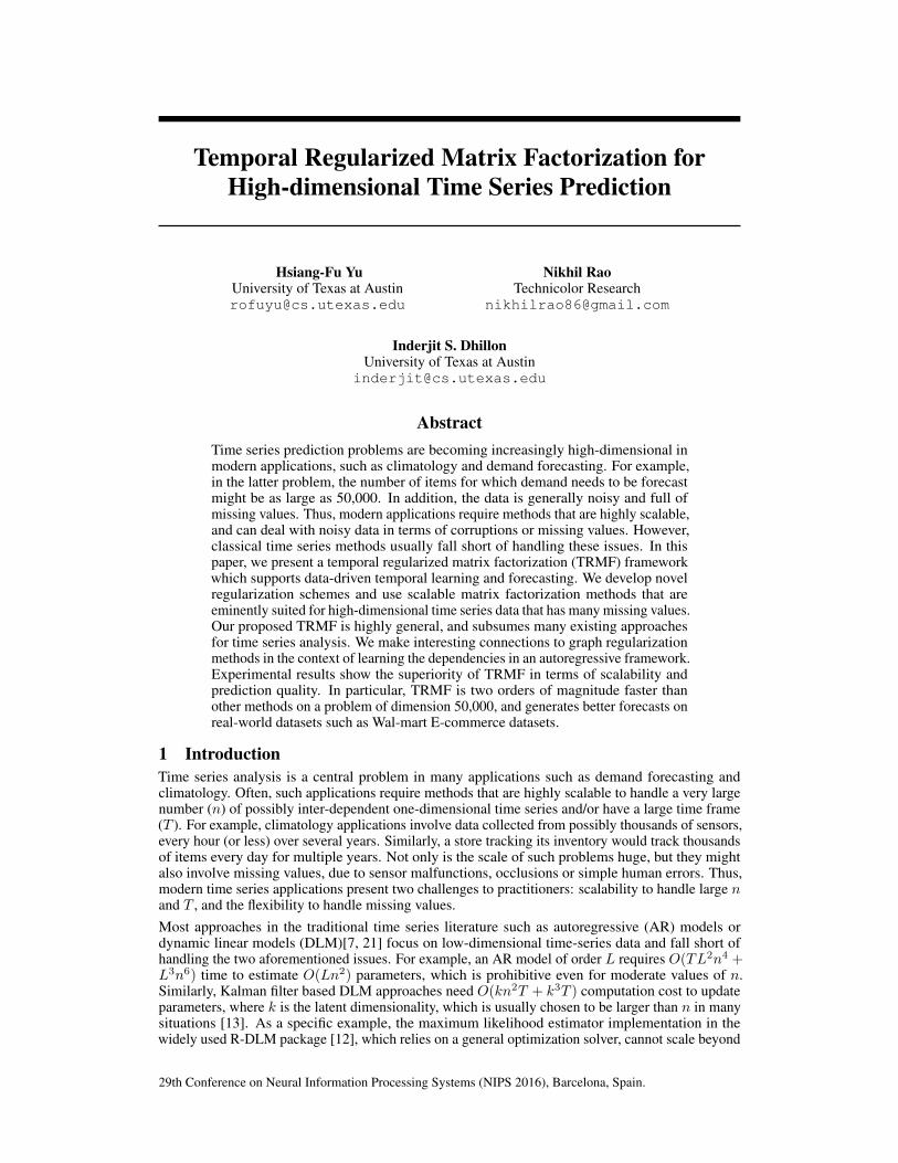
n in the tens. (See Appendix D for details). On the other hand, for models such as AR, the flexibilityto handle missing values can be challenging even for one-dimensional time series [1], let alone thedifficulty to handle high dimensional time series.A natural way to model high-dimensional time series data is in the form of a matrix, with rowscorresponding to each one-dimensional time series and columns corresponding to time points. In lightof the observation that n time series are usually highly correlated with each other, there have beensome attempts to apply low-rank matrix factorization (MF) or matrix completion (MC) techniquesto analyze high-dimensional time series [2, 14, 16, 23, 26]. Unlike the AR and DLM models above,state-of-the-art MF methods scale linearly in n, and hence can handle large datasets. Let Y ∈ Rn×Tbe the matrix for the observed n-dimensional time series with Yit being the observation at the t-thtime point of the i-th time series. Under the standard MF approach, Yit is estimated by the innerproduct f>i xt, where fi ∈ Rk is a k-dimensional latent embedding for the i-th time series, andxt ∈ Rk is a k-dimensional latent temporal embedding for the t-th time point. We can stack thext into the columns of a matrix X ∈ Rk×T and f>i into the rows of F ∈ Rn×k (Figure 1) to getY ≈ FX . We can then solve:
minF,X
∑(i,t)∈Ω
(Yit − f>i xt
)2+ λfRf (F ) + λxRx(X), (1)
Item
s
Y
Time
≈ F
X
Time- dependent variables
f>i
xt
Ynew
Xnew
Figure 1: Matrix Factorization model for mul-tiple time series. F captures features for eachtime series in the matrix Y , and X capturesthe latent and time-varying variables.
where Ω is the set of the observed entries. Rf (F ),Rx(X) are regularizers for F and X , which usu-ally play a role to avoid overfitting and/or to en-courage some specific temporal structures amongthe embeddings. It is clear that the common choiceof the regularizer Rx(X) = ‖X‖F is no longerappropriate for time series applications, as it doesnot take into account the ordering among the tem-poral embeddings xt. Most existing MF ap-proaches [2, 14, 16, 23, 26] adapt graph-based ap-proaches to handle temporal dependencies. Specif-ically, the dependencies are described by a weighted similarity graph and incorporated through aLaplacian regularizer [18]. However, such graph-based regularization fails in cases where there arenegative correlations between two time points. Furthermore, unlike scenarios where explicit graphinformation is available with the data (such as a social network or product co-purchasing graphfor recommender systems), explicit temporal dependency structure is usually unavailable and hasto be inferred or approximated, which causes practitioners to either perform a separate procedureto estimate the dependencies or consider very short-term dependencies with simple fixed weights.Moreover, existing MF approaches, while yielding good estimations for missing values in past points,are poor in terms of forecasting future values, which is the problem of interest in time series analysis.In this paper, we propose a novel temporal regularized matrix factorization framework (TRMF) forhigh-dimensional time series analysis. In TRMF, we consider a principled approach to describe thestructure of temporal dependencies among latent temporal embeddings xt and design a temporalregularizer to incorporate this temporal structure into the standard MF formulation. Unlike mostexisting MF approaches, our TRMF method supports data-driven temporal dependency learningand also brings the ability to forecast future values to a matrix factorization approach. In addition,inherited from the property of MF approaches, TRMF can easily handle high-dimensional time seriesdata even in the presence of many missing values. As a specific example, we demonstrate a novelautoregressive temporal regularizer which encourages AR structure among temporal embeddingsxt. We also make connections between the proposed regularization framework and graph-basedapproaches [18], where even negative correlations can be accounted for. This connection not onlyleads to better understanding about the dependency structure incorporated by our framework but alsobrings the benefit of using off-the-shelf efficient solvers such as GRALS [15] directly to solve TRMF.Paper Organization. In Section 2, we review the existing approaches and their limitations on datawith temporal dependencies. We present the proposed TRMF framework in Section 3, and show thatthe method is highly general and can be used for a variety of time series applications. We introducea novel AR temporal regularizer in Section 4, and make connections to graph-based regularizationapproaches. We demonstrate the superiority of the proposed approach via extensive experimentalresults in Section 5 and conclude the paper in Section 6.
2
2 Motivations: Existing Approaches and Limitations2.1 Classical Time-Series ModelsModels such as AR and DLM are not suitable for modern multiple high-dimensional time series data(i.e., both n and T are large) due to their inherent computational inefficiency (see Section 1). To avoidoverfitting in AR models, there have been studies with various structured transition matrices suchas low rank and sparse matrices [5, 10, 11]. The focus of this research has been on obtaining betterstatistical guarantees. The scalability issue of AR models remains open. On the other hand, it is alsochallenging for many classic time-series models to deal with data that has many missing values [1].In many situations where the model parameters are either given or designed by practitioners, theKalman filter approach is used to perform forecasting, while the Kalman smoothing approach isused to impute missing entries. When model parameters are unknown, EM algorithms are applied toestimate both the model parameters and latent embeddings for DLM [3, 8, 9, 17, 19]. As most EMapproaches for DLM contain the Kalman filter as a building block, they cannot scale to very highdimensional time series data. Indeed, as shown in Section 5, the popular R package for DLM’s doesnot scale beyond data with tens of dimensions.2.2 Existing Matrix Factorization Approaches for Data with Temporal DependenciesIn standard MF (1), the squared Frobenius norm Rx(X) = ‖X‖2F =
∑Tt=1‖xt‖
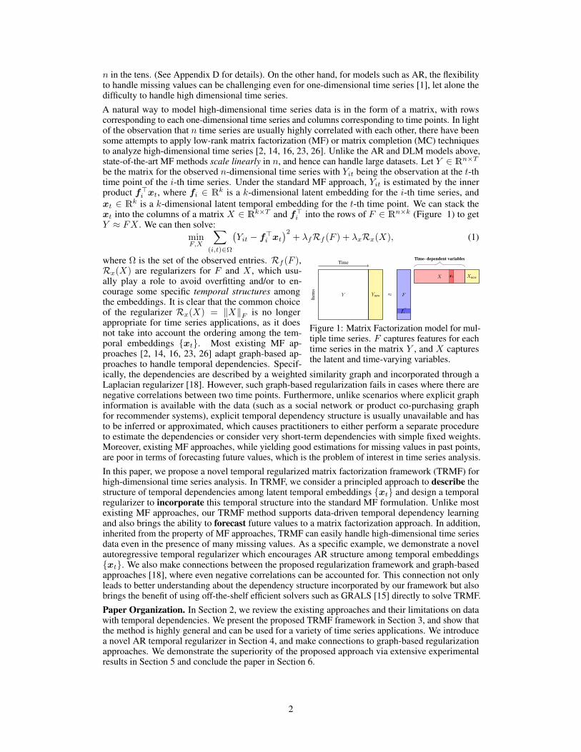
2 is usually theregularizer of choice for X . Because squared Frobenius norm assumes no dependencies among xt,standard MF formulation is invariant to column permutation and not applicable to data with temporaldependencies. Hence most existing temporal MF approaches turn to the framework of graph-basedregularization [18] for temporally dependent xt, with a graph encoding the temporal dependencies.An exception is the work in [22], where the authors use specially designed regularizers to encouragea log-normal structure on the temporal coefficients.Graph regularization for temporal dependencies:The framework of graph-based regularization isan approach to describe and incorporate general dependencies among variables. Let G be a graphover xt and Gts be the edge weight between the t-th node and s-th node. A popular regularizer toinclude as part of an objective function is the following:
Rx(X) = G(X | G, η) := 1
2
∑t∼s
Gts‖xt − xs‖2 +η
2
∑t
‖xt‖2, (2)
tt− 1t− 2t− 3t− 4 t+ 1· · · · · ·w1
w4
w1
w4
w1w1w1
Figure 2: Graph-based regularization for tem-poral dependencies.
where t ∼ s denotes an edge between t-th node ands-th node, and the second summation term is used toguarantee strong convexity. A large Gts will ensurethat xt and xs are close to each other in Euclideandistance, when (2) is minimized. Note that to guaran-tee the convexity of G(X | G, η), we need Gts ≥ 0.To apply graph-based regularizers to temporal dependencies, we need to specify the (repeating)dependency pattern by a lag set L and a weight vector w such that all the edges t ∼ s of distancel (i.e., |s− t| = l) share the same weight Gts = wl. See Figure 2 for an example with L = 1, 4.Given L and w, the corresponding graph regularizer becomes
G(X | G, η)= 1
2
∑l∈L
∑t:t>l
wl(xt − xt−l)2 +
η
2
∑t
‖xt‖2. (3)
This direct use of graph-based approach, while intuitive, has two issues: a) there might be negativelycorrelated dependencies between two time points; b) unlike many applications where such regularizersare used, the explicit temporal dependency structure is usually not available and has to be inferred.As a result, most existing approaches consider only very simple temporal dependencies such as asmall size of L (e.g., L = 1) and/or uniform weights (e.g., wl = 1, ∀l ∈ L). For example, asimple chain graph is considered to design the smoothing regularizer in TCF [23]. This leads to poorforecasting abilities of existing MF methods for large-scale time series applications.2.3 Challenges to Learn Temporal DependenciesOne could try to learn the weights wl automatically, by using the same regularizer as in (3) but withthe weights unknown. This would lead to the following optimization problem:
minF,X,w≥0
∑(i,t)∈Ω
(Yit − f>i xt
)2+λfRf (F )+
λx2
∑l∈L
∑t:t−l>0
wl(xt − xt−l)2+λxη
2
∑t
‖xt‖2, (4)
where w ≥ 0 (0 being the zero vector) is the constraint imposed by typical graph regularization.
3
It is not hard to see that the above optimization yields the trivial all-zero solution for w∗, meaningthe objective function is minimized when no temporal dependencies exist! To avoid the all zerosolution, one might want to impose a simplex constraint on w (i.e.,
∑l∈L wl = 1). Again, it
is not hard to see that this will result in w∗ being a 1-sparse vector, with wl∗ being 1, wherel∗ = arg minl∈L
∑t:t>l ‖xt − xt−l‖2. Thus, looking to learn the weights automatically by simply
plugging in the regularizer in the MF formulation is not a viable option.
3 Temporal Regularized Matrix FactorizationIn order to resolve the limitations mentioned in Sections 2.2 and 2.3, we propose the TemporalRegularized Matrix Factorization (TRMF) framework, which is a novel approach to incorporatetemporal dependencies into matrix factorization models. Unlike the aforementioned graph-basedapproaches, we propose to use well-studied time series models to describe temporal dependenciesamong xt explicitly. Such models take the form:
xt = MΘ(xt−l : l ∈ L) + εt, (5)where εt is a Gaussian noise vector, and MΘ is the time-series model parameterized by L and Θ. Lis a set containing the lag indices l, denoting a dependency between t-th and (t− l)-th time points,while Θ captures the weighting information of temporal dependencies (such as the transition matrixin AR models). To incorporate the temporal dependency into the standard MF formulation (1), wepropose to design a new regularizer TM(X | Θ) which encourages the structure induced by MΘ.Taking a standard approach to model time series, we set TM(X | Θ) be the negative log likelihood ofobserving a particular realization of the xt for a given model MΘ:
TM(X | Θ) = − logP(x1, . . . ,xT | Θ). (6)When Θ is given, we can useRx(X) = TM(X | Θ) in the MF formulation (1) to encourage xt tofollow the temporal dependency induced by MΘ. When the Θ is unknown, we can treat Θ as anotherset of variables and include another regularizerRθ(Θ) into (1):
minF,X,Θ
∑(i,t)∈Ω
(Yit − f>i xt
)2+ λfRf (F ) + λxTM(X | Θ) + λθRθ(Θ), (7)
which be solved by an alternating minimization procedure over F , X , and Θ.Data-driven Temporal Dependency Learning in TRMF:Recall that in Section 2.3, we showedthat directly using graph based regularizers to incorporate temporal dependencies leads to trivialsolutions for the weights. TRMF circumvents this issue. When F and X are fixed, (7) is reduced to:
minΘ
λxTM(X | Θ) + λθRθ(Θ), (8)
which is a maximum-a-posterior (MAP) estimation problem (in the Bayesian sense) to estimate thebest Θ for a given xt under the MΘ model. There are well-developed algorithms to solve (8) andobtain non-trivial Θ. Thus, unlike most existing temporal matrix factorization approaches where thestrength of dependencies is fixed, Θ in TRMF can be learned automatically from data.Time Series Analysis with TRMF:We can see that TRMF (7) lends itself seamlessly to handle avariety of commonly encountered tasks in analyzing data with temporal dependency:• Time-series Forecasting: Once we have MΘ for latent embeddings xt : 1, . . . , T, we can
use it to predict future latent embeddings xt : t > T and have the ability to obtain non-trivialforecasting results for yt = Fxt for t > T .
• Missing-value Imputation: In some time-series applications, some entries in Y might be unob-served, for example, due to faulty sensors in electricity usage monitoring or occlusions in thecase of motion recognition in video. We can use f>i xt to impute these missing entries, much likestandard matrix completion, that is used in recommender systems [23] and sensor networks [26].
Extensions to Incorporate Extra Information:Like matrix factorization, TRMF (7) can be ex-tended to incorporate additional information. For example, pairwise relationships between the timeseries can be incorporated using structural regularizers on F . Furthermore, when features are knownfor the time series, we can make use of interaction models such as those in [6, 24, 25]. Also, TRMFcan be extended to tensors. More details on these extensions can be found in Appendix B.
4 A Novel Autoregressive Temporal RegularizerIn Section 3, we described the TRMF framework in a very general sense, with the regularizerTM(X | Θ) incorporating dependencies specified by the time series model MΘ. In this section,we specialize this to the case of AR models, which are parameterized by a lag set L and weightsW =
W (l) ∈ Rk×k : l ∈ L
. Assume that xt is a noisy linear combination of some previous
4
points; that is, xt =∑l∈LW
(l)xt−l + εt, where εt is a Gaussian noise vector. For simplicity, weassume that εt ∼ N (0, σ2Ik), where Ik is the k × k identity matrix1. The temporal regularizerTM(X | Θ) corresponding to this AR model can be written as:
TAR(X |L,W, η) :=1
2
T∑t=m
∥∥∥∥∥xt −∑l∈L
W (l)xt−l
∥∥∥∥∥2
+η
2
∑t
‖xt‖2, (9)
where m := 1 + L, L := max(L), and η > 0 to guarantee the strong convexity of (9).
TRMF allows us to learn the weightsW (l)
when they are unknown. Since each W (l) ∈ Rk×k,
there will be |L|k2 variables to learn, which may lead to overfitting. To prevent this and to yieldmore interpretable results, we consider diagonal W (l), reducing the number of parameters to |L|k.To simplify notation, we use W to denote the k × L matrix where the l-th column constitutesthe diagonal elements of W (l). Note that for l /∈ L, the l-th column of W is a zero vector. Letx>r = [· · · , Xrt, · · · ] be the r-th row of X and w>r = [· · · ,Wrl, · · · ] be the r-th row ofW . Then(9) can be written as TAR(X |L,W, η) =
∑kr=1 TAR(xr |L, wr, η), where we define
TAR(x |L, w, η) =1
2
T∑t=m
(xt −
∑l∈L
wlxt−l
)2
+η
2‖x‖2, (10)
with xt being the t-th element of x, and wl being the l-th element of w.Correlations among Multiple Time Series. Even when
W l
is diagonal, TRMF retains the powerto capture the correlations among time series via the factors fi, since diagonal
W l
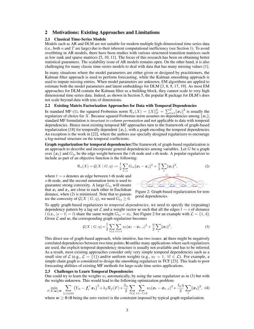
has an effectonly on the structure of latent embeddings xt. Indeed, as the i-th dimension of yt is modeledby f>i X in (7), the low rank F is a k dimensional latent embedding of multiple time series. Thisembedding captures correlations among multiple time series. Furthermore, fi, acting as time seriesfeatures, can be used to perform classification/clustering even in the presence of missing values.Choice of Lag Index Set L. Unlike most approaches mentioned in Section 2.2, the choice of L inTRMF is more flexible. Thus, TRMF can provide important advantages: First, because there is noneed to specify the weight parametersW , L can be chosen to be larger to account for long rangedependencies, which also yields more accurate and robust forecasts. Second, the indices in L need notbe continuous so that one can easily embed domain knowledge about periodicity or seasonality. Forexample, one might consider L = 1, 2, 3, 51, 52, 53 for weekly data with a one year seasonality.Connections to Graph Regularization. We now establish connections between TAR(x |L, w, η)and graph regularization (2) for matrix factorization. Let L := L ∪ 0, w0 = −1 so that (10) is
TAR(x |L, w, η) =1
2
T∑t=m
∑l∈L
wlxt−l
2
+η
2‖x‖2,
and let δ(d) :=l ∈ L : l − d ∈ L
. We then have the following result:
Theorem 1. Given a lag index set L, weight vector w ∈ RL, and x ∈ RT , there is a weightedsigned graph GAR with T nodes and a diagonal matrix D ∈ RT×T such that
TAR(x |L, w, η) = G(x | GAR, η
)+
1
2x>Dx, (11)
where G(x | GAR, η
)is the graph regularization (2) with G = GAR. Furthermore, ∀t and d
GARt,t+d =
∑l∈δ(d)
∑m≤t+l≤T
−wlwl−d if δ(d) 6= φ,
0 otherwise,and Dtt =
∑l∈L
wl
∑l∈L
wl[m ≤ t+ l ≤ T ]
tt− 1t− 2t− 3t− 4 t+ 1· · · · · ·w1
w4
−w1w4−w1w4 −w1w4
w1
w4
w1w1w1
Figure 3: The graph structure induced by the ARtemporal regularizer (10) with L = 1, 4.
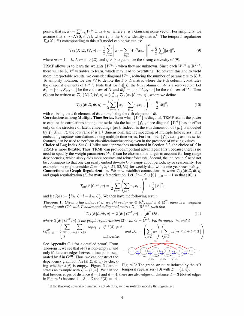
See Appendix C.1 for a detailed proof. FromTheorem 1, we see that δ(d) is non-empty if andonly if there are edges between time points sep-arated by d in GAR. Thus, we can construct thedependency graph for TAR(x |L, w, η) by check-ing whether δ(d) is empty. Figure 3 demon-strates an example with L = 1, 4. We can seethat besides edges of distance d = 1 and d = 4, there are also edges of distance d = 3 (dotted edgesin Figure 3) because 4− 3 ∈ L and δ(3) = 4.
1If the (known) covariance matrix is not identity, we can suitably modify the regularizer.
5
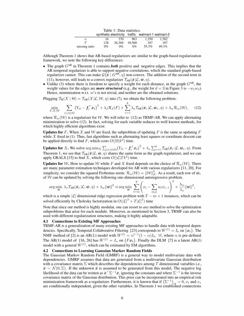
Table 1: Data statistics.synthetic electricity traffic walmart-1 walmart-2
n 16 370 963 1,350 1,582T 128 26,304 10,560 187 187
missing ratio 0% 0% 0% 55.3% 49.3%
Although Theorem 1 shows that AR-based regularizers are similar to the graph-based regularizationframework, we note the following key differences:• The graph GAR in Theorem 1 contains both positive and negative edges. This implies that the
AR temporal regularizer is able to support negative correlations, which the standard graph-basedregularizer cannot. This can make G
(x | GAR, η
)non-convex. The addition of the second term in
(11), however, still leads to a convex regularizer TAR(x |L, w, η).• Unlike (3) where there is freedom to specify a weight for each distance, in the graph GAR, the
weight values for the edges are more structured (e.g., the weight for d = 3 in Figure 3 is −w1w4).Hence, minimization w.r.t. w′s is not trivial, and neither are the obtained solutions.
Plugging TM(X | Θ) = TAR(X |L,W, η) into (7), we obtain the following problem:
minF,X,W
∑(i,t)∈Ω
(Yit − f>i xt
)2+ λfRf (F ) +
k∑r=1
λxTAR(xr |L, wr, η) + λwRw(W), (12)
whereRw(W) is a regularizer forW . We will refer to (12) as TRMF-AR. We can apply alternatingminimization to solve (12). In fact, solving for each variable reduces to well known methods, forwhich highly efficient algorithms exist:Updates for F . When X andW are fixed, the subproblem of updating F is the same as updating Fwhile X fixed in (1). Thus, fast algorithms such as alternating least squares or coordinate descent canbe applied directly to find F , which costs O(|Ω|k2) time.
Updates for X . We solve arg minX∑
(i,t)∈Ω
(Yit − f>i xt
)2+ λx
∑kr=1 TAR(xr |L, wr, η). From
Theorem 1, we see that TAR(x |L, w, η) shares the same form as the graph regularizer, and we canapply GRALS [15] to find X , which costs O(|L|Tk2) time.Updates forW . How to updateW while F and X fixed depends on the choice ofRw(W). Thereare many parameter estimation techniques developed for AR with various regularizers [11, 20]. Forsimplicity, we consider the squared Frobenius norm: Rw(W) = ‖W‖2F . As a result, each row of wrofW can be updated by solving the following one-dimensional autoregressive problem.
arg minw
λxTAR(xr |L, w, η) + λw‖w‖2 ≡ arg minw
T∑t=m
(xt −
∑l∈L
wlxt−l
)2
+λwλx‖w‖2,
which is a simple |L| dimensional ridge regression problem with T −m+ 1 instances, which can besolved efficiently by Cholesky factorization in O(|L|3 + T |L|2) timeNote that since our method is highly modular, one can resort to any method to solve the optimizationsubproblems that arise for each module. Moreover, as mentioned in Section 3, TRMF can also beused with different regularization structures, making it highly adaptable.4.1 Connections to Existing MF ApproachesTRMF-AR is a generalization of many existing MF approaches to handle data with temporal depen-dencies. Specifically, Temporal Collaborative Filtering [23] corresponds to W (1) = Ik on xt. TheNMF method of [2] is an AR(L) model with W (l) = αl−1(1 − α)Ik, ∀l, where α is pre-defined.The AR(1) model of [16, 26] has W (1) = In on Fxt. Finally the DLM [7] is a latent AR(1)model with a general W (1), which can be estimated by EM algorithms.4.2 Connections to Learning Gaussian Markov Random FieldsThe Gaussian Markov Random Field (GMRF) is a general way to model multivariate data withdependencies. GMRF assumes that data are generated from a multivariate Gaussian distributionwith a covariance matrix Σ which describes the dependencies among T dimensional variables i.e.,x ∼ N (0,Σ). If the unknown x is assumed to be generated from this model, The negative loglikelihood of the data can be written as x>Σ−1x, ignoring the constants and where Σ−1 is the inversecovariance matrix of the Gaussian distribution. This prior can be incorporated into an empirical riskminimization framework as a regularizer. Furthermore, it is known that if
(Σ−1
)st
= 0, xt and xsare conditionally independent, given the other variables. In Theorem 1 we established connections
6
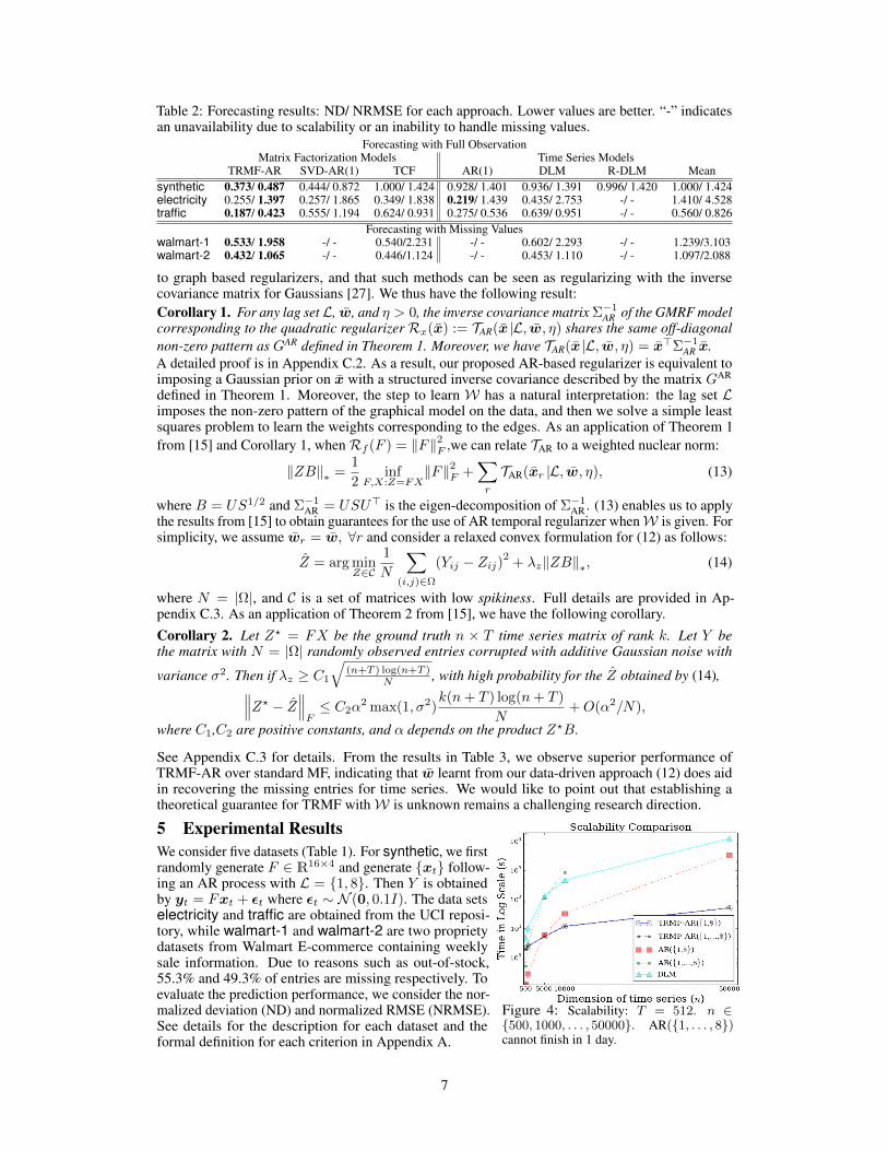
Table 2: Forecasting results: ND/ NRMSE for each approach. Lower values are better. “-” indicatesan unavailability due to scalability or an inability to handle missing values.
Forecasting with Full ObservationMatrix Factorization Models Time Series Models
TRMF-AR SVD-AR(1) TCF AR(1) DLM R-DLM Meansynthetic 0.373/ 0.487 0.444/ 0.872 1.000/ 1.424 0.928/ 1.401 0.936/ 1.391 0.996/ 1.420 1.000/ 1.424electricity 0.255/ 1.397 0.257/ 1.865 0.349/ 1.838 0.219/ 1.439 0.435/ 2.753 -/ - 1.410/ 4.528traffic 0.187/ 0.423 0.555/ 1.194 0.624/ 0.931 0.275/ 0.536 0.639/ 0.951 -/ - 0.560/ 0.826
Forecasting with Missing Valueswalmart-1 0.533/ 1.958 -/ - 0.540/2.231 -/ - 0.602/ 2.293 -/ - 1.239/3.103walmart-2 0.432/ 1.065 -/ - 0.446/1.124 -/ - 0.453/ 1.110 -/ - 1.097/2.088
to graph based regularizers, and that such methods can be seen as regularizing with the inversecovariance matrix for Gaussians [27]. We thus have the following result:Corollary 1. For any lag setL, w, and η > 0, the inverse covariance matrix Σ−1
AR of the GMRF modelcorresponding to the quadratic regularizerRx(x) := TAR(x |L, w, η) shares the same off-diagonalnon-zero pattern as GAR defined in Theorem 1. Moreover, we have TAR(x |L, w, η) = x>Σ−1
AR x.A detailed proof is in Appendix C.2. As a result, our proposed AR-based regularizer is equivalent toimposing a Gaussian prior on x with a structured inverse covariance described by the matrix GAR
defined in Theorem 1. Moreover, the step to learn W has a natural interpretation: the lag set Limposes the non-zero pattern of the graphical model on the data, and then we solve a simple leastsquares problem to learn the weights corresponding to the edges. As an application of Theorem 1from [15] and Corollary 1, whenRf (F ) = ‖F‖2F ,we can relate TAR to a weighted nuclear norm:
‖ZB‖∗ =1
2inf
F,X:Z=FX‖F‖2F +
∑r
TAR(xr |L, w, η), (13)
where B = US1/2 and Σ−1AR = USU> is the eigen-decomposition of Σ−1
AR . (13) enables us to applythe results from [15] to obtain guarantees for the use of AR temporal regularizer whenW is given. Forsimplicity, we assume wr = w, ∀r and consider a relaxed convex formulation for (12) as follows:
Z = arg minZ∈C
1
N
∑(i,j)∈Ω
(Yij − Zij)2+ λz‖ZB‖∗, (14)
where N = |Ω|, and C is a set of matrices with low spikiness. Full details are provided in Ap-pendix C.3. As an application of Theorem 2 from [15], we have the following corollary.Corollary 2. Let Z? = FX be the ground truth n × T time series matrix of rank k. Let Y bethe matrix with N = |Ω| randomly observed entries corrupted with additive Gaussian noise with
variance σ2. Then if λz ≥ C1
√(n+T ) log(n+T )
N , with high probability for the Z obtained by (14),∥∥∥Z? − Z∥∥∥F≤ C2α
2 max(1, σ2)k(n+ T ) log(n+ T )
N+O(α2/N),
where C1,C2 are positive constants, and α depends on the product Z?B.
See Appendix C.3 for details. From the results in Table 3, we observe superior performance ofTRMF-AR over standard MF, indicating that w learnt from our data-driven approach (12) does aidin recovering the missing entries for time series. We would like to point out that establishing atheoretical guarantee for TRMF withW is unknown remains a challenging research direction.
5 Experimental Results
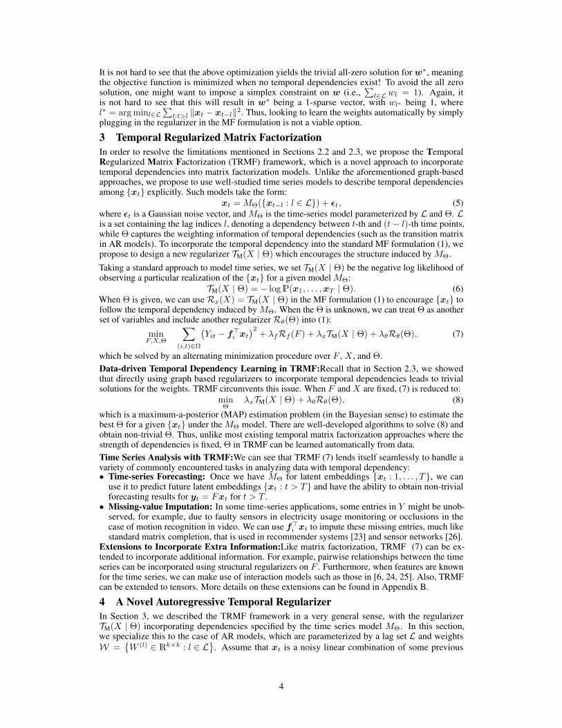
Figure 4: Scalability: T = 512. n ∈500, 1000, . . . , 50000. AR(1, . . . , 8)cannot finish in 1 day.
We consider five datasets (Table 1). For synthetic, we firstrandomly generate F ∈ R16×4 and generate xt follow-ing an AR process with L = 1, 8. Then Y is obtainedby yt = Fxt + εt where εt ∼ N (0, 0.1I). The data setselectricity and traffic are obtained from the UCI reposi-tory, while walmart-1 and walmart-2 are two proprietydatasets from Walmart E-commerce containing weeklysale information. Due to reasons such as out-of-stock,55.3% and 49.3% of entries are missing respectively. Toevaluate the prediction performance, we consider the nor-malized deviation (ND) and normalized RMSE (NRMSE).See details for the description for each dataset and theformal definition for each criterion in Appendix A.
7
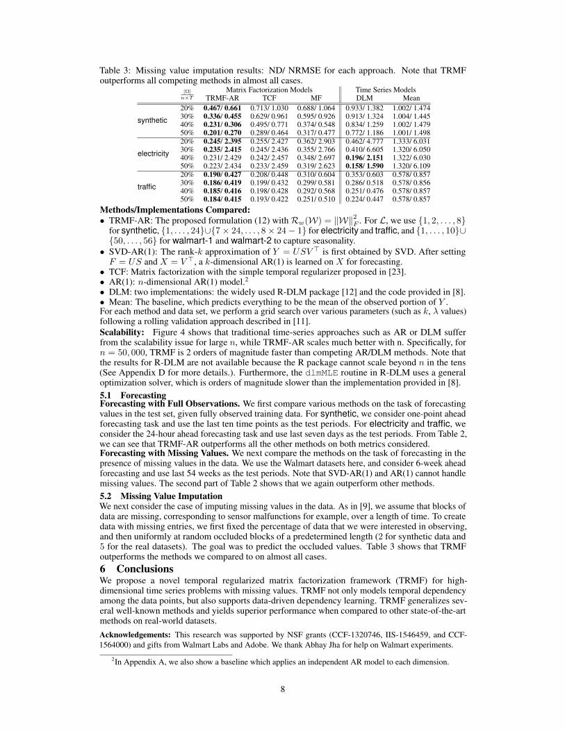
Table 3: Missing value imputation results: ND/ NRMSE for each approach. Note that TRMFoutperforms all competing methods in almost all cases.
|Ω|n×T
Matrix Factorization Models Time Series ModelsTRMF-AR TCF MF DLM Mean
synthetic
20% 0.467/ 0.661 0.713/ 1.030 0.688/ 1.064 0.933/ 1.382 1.002/ 1.47430% 0.336/ 0.455 0.629/ 0.961 0.595/ 0.926 0.913/ 1.324 1.004/ 1.44540% 0.231/ 0.306 0.495/ 0.771 0.374/ 0.548 0.834/ 1.259 1.002/ 1.47950% 0.201/ 0.270 0.289/ 0.464 0.317/ 0.477 0.772/ 1.186 1.001/ 1.498
electricity
20% 0.245/ 2.395 0.255/ 2.427 0.362/ 2.903 0.462/ 4.777 1.333/ 6.03130% 0.235/ 2.415 0.245/ 2.436 0.355/ 2.766 0.410/ 6.605 1.320/ 6.05040% 0.231/ 2.429 0.242/ 2.457 0.348/ 2.697 0.196/ 2.151 1.322/ 6.03050% 0.223/ 2.434 0.233/ 2.459 0.319/ 2.623 0.158/ 1.590 1.320/ 6.109
traffic
20% 0.190/ 0.427 0.208/ 0.448 0.310/ 0.604 0.353/ 0.603 0.578/ 0.85730% 0.186/ 0.419 0.199/ 0.432 0.299/ 0.581 0.286/ 0.518 0.578/ 0.85640% 0.185/ 0.416 0.198/ 0.428 0.292/ 0.568 0.251/ 0.476 0.578/ 0.85750% 0.184/ 0.415 0.193/ 0.422 0.251/ 0.510 0.224/ 0.447 0.578/ 0.857
Methods/Implementations Compared:• TRMF-AR: The proposed formulation (12) withRw(W) = ‖W‖2F . For L, we use 1, 2, . . . , 8
for synthetic, 1, . . . , 24∪7× 24, . . . , 8× 24− 1 for electricity and traffic, and 1, . . . , 10∪50, . . . , 56 for walmart-1 and walmart-2 to capture seasonality.
• SVD-AR(1): The rank-k approximation of Y = USV > is first obtained by SVD. After settingF = US and X = V >, a k-dimensional AR(1) is learned on X for forecasting.
• TCF: Matrix factorization with the simple temporal regularizer proposed in [23].• AR(1): n-dimensional AR(1) model.2• DLM: two implementations: the widely used R-DLM package [12] and the code provided in [8].• Mean: The baseline, which predicts everything to be the mean of the observed portion of Y .For each method and data set, we perform a grid search over various parameters (such as k, λ values)following a rolling validation approach described in [11].Scalability: Figure 4 shows that traditional time-series approaches such as AR or DLM sufferfrom the scalability issue for large n, while TRMF-AR scales much better with n. Specifically, forn = 50, 000, TRMF is 2 orders of magnitude faster than competing AR/DLM methods. Note thatthe results for R-DLM are not available because the R package cannot scale beyond n in the tens(See Appendix D for more details.). Furthermore, the dlmMLE routine in R-DLM uses a generaloptimization solver, which is orders of magnitude slower than the implementation provided in [8].5.1 ForecastingForecasting with Full Observations. We first compare various methods on the task of forecastingvalues in the test set, given fully observed training data. For synthetic, we consider one-point aheadforecasting task and use the last ten time points as the test periods. For electricity and traffic, weconsider the 24-hour ahead forecasting task and use last seven days as the test periods. From Table 2,we can see that TRMF-AR outperforms all the other methods on both metrics considered.Forecasting with Missing Values. We next compare the methods on the task of forecasting in thepresence of missing values in the data. We use the Walmart datasets here, and consider 6-week aheadforecasting and use last 54 weeks as the test periods. Note that SVD-AR(1) and AR(1) cannot handlemissing values. The second part of Table 2 shows that we again outperform other methods.5.2 Missing Value ImputationWe next consider the case of imputing missing values in the data. As in [9], we assume that blocks ofdata are missing, corresponding to sensor malfunctions for example, over a length of time. To createdata with missing entries, we first fixed the percentage of data that we were interested in observing,and then uniformly at random occluded blocks of a predetermined length (2 for synthetic data and5 for the real datasets). The goal was to predict the occluded values. Table 3 shows that TRMFoutperforms the methods we compared to on almost all cases.6 ConclusionsWe propose a novel temporal regularized matrix factorization framework (TRMF) for high-dimensional time series problems with missing values. TRMF not only models temporal dependencyamong the data points, but also supports data-driven dependency learning. TRMF generalizes sev-eral well-known methods and yields superior performance when compared to other state-of-the-artmethods on real-world datasets.Acknowledgements: This research was supported by NSF grants (CCF-1320746, IIS-1546459, and CCF-1564000) and gifts from Walmart Labs and Adobe. We thank Abhay Jha for help on Walmart experiments.
2In Appendix A, we also show a baseline which applies an independent AR model to each dimension.
8
References[1] O. Anava, E. Hazan, and A. Zeevi. Online time series prediction with missing data. In Proceedings of the
International Conference on Machine Learning, pages 2191–2199, 2015.[2] Z. Chen and A. Cichocki. Nonnegative matrix factorization with temporal smoothness and/or spatial
decorrelation constraints. Laboratory for Advanced Brain Signal Processing, RIKEN, Tech. Rep, 68, 2005.[3] Z. Ghahramani and G. E. Hinton. Parameter estimation for linear dynamical systems. Technical report,
Technical Report CRG-TR-96-2, University of Totronto, Dept. of Computer Science, 1996.[4] R. L. Graham, D. E. Knuth, and O. Patashnik. Concrete Mathematics: A Foundation for Computer Science.
Addison-Wesley Longman Publishing Co., Inc., 2nd edition, 1994.[5] F. Han and H. Liu. Transition matrix estimation in high dimensional time series. In Proceedings of the
International Conference on Machine Learning, pages 172–180, 2013.[6] P. Jain and I. S. Dhillon. Provable inductive matrix completion. arXiv preprint arXiv:1306.0626, 2013.[7] R. E. Kalman. A new approach to linear filtering and prediction problems. Journal of Fluids Engineering,
82(1):35–45, 1960.[8] L. Li and B. A. Prakash. Time series clustering: Complex is simpler! In Proceedings of the International
Conference on Machine Learning, pages 185–192, 2011.[9] L. Li, J. McCann, N. S. Pollard, and C. Faloutsos. DynaMMo: Mining and summarization of coevolving
sequences with missing values. In ACM SIGKDD International Conference on Knowledge discovery anddata mining, pages 507–516. ACM, 2009.
[10] I. Melnyk and A. Banerjee. Estimating structured vector autoregressive model. In Proceedings of theThirty Third International Conference on Machine Learning (ICML), 2016.
[11] W. B. Nicholson, D. S. Matteson, and J. Bien. Structured regularization for large vector autoregressions.Technical report, Technical Report, University of Cornell, 2014.
[12] G. Petris. An R package for dynamic linear models. Journal of Statistical Software, 36(12):1–16, 2010.[13] G. Petris, S. Petrone, and P. Campagnoli. Dynamic Linear Models with R. Use R! Springer, 2009.[14] S. Rallapalli, L. Qiu, Y. Zhang, and Y.-C. Chen. Exploiting temporal stability and low-rank structure
for localization in mobile networks. In International Conference on Mobile Computing and Networking,MobiCom ’10, pages 161–172. ACM, 2010.
[15] N. Rao, H.-F. Yu, P. K. Ravikumar, and I. S. Dhillon. Collaborative filtering with graph information:Consistency and scalable methods. In Advances in Neural Information Processing Systems 27, 2015.
[16] M. Roughan, Y. Zhang, W. Willinger, and L. Qiu. Spatio-temporal compressive sensing and internet trafficmatrices (extended version). IEEE/ACM Transactions on Networking, 20(3):662–676, June 2012.
[17] R. H. Shumway and D. S. Stoffer. An approach to time series smoothing and forecasting using the EMalgorithm. Journal of time series analysis, 3(4):253–264, 1982.
[18] A. J. Smola and R. Kondor. Kernels and regularization on graphs. In Learning theory and kernel machines,pages 144–158. Springer, 2003.
[19] J. Z. Sun, K. R. Varshney, and K. Subbian. Dynamic matrix factorization: A state space approach. InProceedings of International Conference on Acoustics, Speech and Signal Processing, pages 1897–1900.IEEE, 2012.
[20] H. Wang, G. Li, and C.-L. Tsai. Regression coefficient and autoregressive order shrinkage and selection viathe lasso. Journal of the Royal Statistical Society: Series B (Statistical Methodology), 69(1):63–78, 2007.
[21] M. West and J. Harrison. Bayesian Forecasting and Dynamic Models. Springer Series in Statistics. Springer,2013.
[22] K. Wilson, B. Raj, and P. Smaragdis. Regularized non-negative matrix factorization with temporaldependencies for speech denoising. In Interspeech, pages 411–414, 2008.
[23] L. Xiong, X. Chen, T.-K. Huang, J. G. Schneider, and J. G. Carbonell. Temporal collaborative filteringwith Bayesian probabilistic tensor factorization. In SIAM International Conference on Data Mining, pages223–234, 2010.
[24] M. Xu, R. Jin, and Z.-H. Zhou. Speedup matrix completion with side information: Application to multi-label learning. In C. Burges, L. Bottou, M. Welling, Z. Ghahramani, and K. Weinberger, editors, Advancesin Neural Information Processing Systems 26, pages 2301–2309, 2013.
[25] H.-F. Yu, P. Jain, P. Kar, and I. S. Dhillon. Large-scale multi-label learning with missing labels. InProceedings of the International Conference on Machine Learning, pages 593–601, 2014.
[26] Y. Zhang, M. Roughan, W. Willinger, and L. Qiu. Spatio-temporal compressive sensing and internet trafficmatrices. SIGCOMM Comput. Commun. Rev., 39(4):267–278, Aug. 2009. ISSN 0146-4833.
[27] T. Zhou, H. Shan, A. Banerjee, and G. Sapiro. Kernelized probabilistic matrix factorization: Exploitinggraphs and side information. In SDM, volume 12, pages 403–414. SIAM, 2012.
9
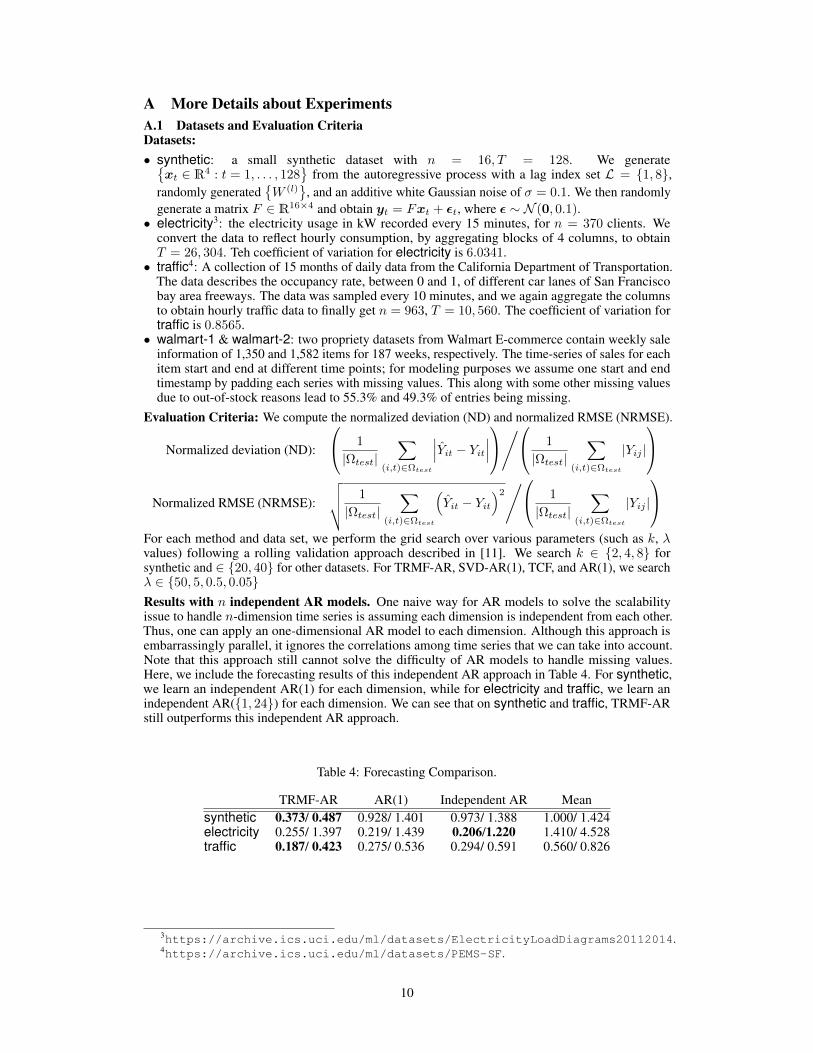
A More Details about ExperimentsA.1 Datasets and Evaluation CriteriaDatasets:• synthetic: a small synthetic dataset with n = 16, T = 128. We generate
xt ∈ R4 : t = 1, . . . , 128
from the autoregressive process with a lag index set L = 1, 8,randomly generated
W (l)
, and an additive white Gaussian noise of σ = 0.1. We then randomly
generate a matrix F ∈ R16×4 and obtain yt = Fxt + εt, where ε ∼ N (0, 0.1).• electricity3: the electricity usage in kW recorded every 15 minutes, for n = 370 clients. We
convert the data to reflect hourly consumption, by aggregating blocks of 4 columns, to obtainT = 26, 304. Teh coefficient of variation for electricity is 6.0341.
• traffic4: A collection of 15 months of daily data from the California Department of Transportation.The data describes the occupancy rate, between 0 and 1, of different car lanes of San Franciscobay area freeways. The data was sampled every 10 minutes, and we again aggregate the columnsto obtain hourly traffic data to finally get n = 963, T = 10, 560. The coefficient of variation fortraffic is 0.8565.
• walmart-1 & walmart-2: two propriety datasets from Walmart E-commerce contain weekly saleinformation of 1,350 and 1,582 items for 187 weeks, respectively. The time-series of sales for eachitem start and end at different time points; for modeling purposes we assume one start and endtimestamp by padding each series with missing values. This along with some other missing valuesdue to out-of-stock reasons lead to 55.3% and 49.3% of entries being missing.
Evaluation Criteria: We compute the normalized deviation (ND) and normalized RMSE (NRMSE).
Normalized deviation (ND):
1
|Ωtest|∑
(i,t)∈Ωtest
∣∣∣Yit − Yit∣∣∣/ 1
|Ωtest|∑
(i,t)∈Ωtest
|Yij |
Normalized RMSE (NRMSE):
√√√√ 1
|Ωtest|∑
(i,t)∈Ωtest
(Yit − Yit
)2/ 1
|Ωtest|∑
(i,t)∈Ωtest
|Yij |
For each method and data set, we perform the grid search over various parameters (such as k, λvalues) following a rolling validation approach described in [11]. We search k ∈ 2, 4, 8 forsynthetic and ∈ 20, 40 for other datasets. For TRMF-AR, SVD-AR(1), TCF, and AR(1), we searchλ ∈ 50, 5, 0.5, 0.05Results with n independent AR models. One naive way for AR models to solve the scalabilityissue to handle n-dimension time series is assuming each dimension is independent from each other.Thus, one can apply an one-dimensional AR model to each dimension. Although this approach isembarrassingly parallel, it ignores the correlations among time series that we can take into account.Note that this approach still cannot solve the difficulty of AR models to handle missing values.Here, we include the forecasting results of this independent AR approach in Table 4. For synthetic,we learn an independent AR(1) for each dimension, while for electricity and traffic, we learn anindependent AR(1, 24) for each dimension. We can see that on synthetic and traffic, TRMF-ARstill outperforms this independent AR approach.
Table 4: Forecasting Comparison.
TRMF-AR AR(1) Independent AR Meansynthetic 0.373/ 0.487 0.928/ 1.401 0.973/ 1.388 1.000/ 1.424electricity 0.255/ 1.397 0.219/ 1.439 0.206/1.220 1.410/ 4.528traffic 0.187/ 0.423 0.275/ 0.536 0.294/ 0.591 0.560/ 0.826
3https://archive.ics.uci.edu/ml/datasets/ElectricityLoadDiagrams20112014.4https://archive.ics.uci.edu/ml/datasets/PEMS-SF.
10
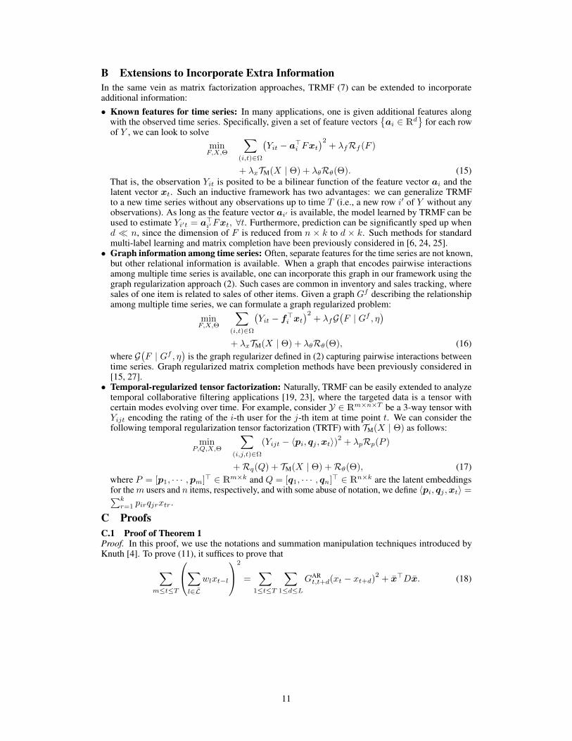
B Extensions to Incorporate Extra InformationIn the same vein as matrix factorization approaches, TRMF (7) can be extended to incorporateadditional information:• Known features for time series: In many applications, one is given additional features along
with the observed time series. Specifically, given a set of feature vectorsai ∈ Rd
for each row
of Y , we can look to solveminF,X,Θ
∑(i,t)∈Ω
(Yit − a>i Fxt
)2+ λfRf (F )
+ λxTM(X | Θ) + λθRθ(Θ). (15)That is, the observation Yit is posited to be a bilinear function of the feature vector ai and thelatent vector xt. Such an inductive framework has two advantages: we can generalize TRMFto a new time series without any observations up to time T (i.e., a new row i′ of Y without anyobservations). As long as the feature vector ai′ is available, the model learned by TRMF can beused to estimate Yi′t = a>i′Fxt, ∀t. Furthermore, prediction can be significantly sped up whend n, since the dimension of F is reduced from n × k to d × k. Such methods for standardmulti-label learning and matrix completion have been previously considered in [6, 24, 25].
• Graph information among time series: Often, separate features for the time series are not known,but other relational information is available. When a graph that encodes pairwise interactionsamong multiple time series is available, one can incorporate this graph in our framework using thegraph regularization approach (2). Such cases are common in inventory and sales tracking, wheresales of one item is related to sales of other items. Given a graph Gf describing the relationshipamong multiple time series, we can formulate a graph regularized problem:
minF,X,Θ
∑(i,t)∈Ω
(Yit − f>i xt
)2+ λfG
(F | Gf , η
)+ λxTM(X | Θ) + λθRθ(Θ), (16)
where G(F | Gf , η
)is the graph regularizer defined in (2) capturing pairwise interactions between
time series. Graph regularized matrix completion methods have been previously considered in[15, 27].
• Temporal-regularized tensor factorization: Naturally, TRMF can be easily extended to analyzetemporal collaborative filtering applications [19, 23], where the targeted data is a tensor withcertain modes evolving over time. For example, consider Y ∈ Rm×n×T be a 3-way tensor withYijt encoding the rating of the i-th user for the j-th item at time point t. We can consider thefollowing temporal regularization tensor factorization (TRTF) with TM(X | Θ) as follows:
minP,Q,X,Θ
∑(i,j,t)∈Ω
(Yijt − 〈pi, qj ,xt〉)2+ λpRp(P )
+Rq(Q) + TM(X | Θ) +Rθ(Θ), (17)where P = [p1, · · · ,pm]> ∈ Rm×k and Q = [q1, · · · , qn]> ∈ Rn×k are the latent embeddingsfor them users and n items, respectively, and with some abuse of notation, we define 〈pi, qj ,xt〉 =∑kr=1 pirqjrxtr.
C ProofsC.1 Proof of Theorem 1Proof. In this proof, we use the notations and summation manipulation techniques introduced byKnuth [4]. To prove (11), it suffices to prove that∑
m≤t≤T
∑l∈L
wlxt−l
2
=∑
1≤t≤T
∑1≤d≤L
GARt,t+d(xt − xt+d)
2+ x>Dx. (18)
11
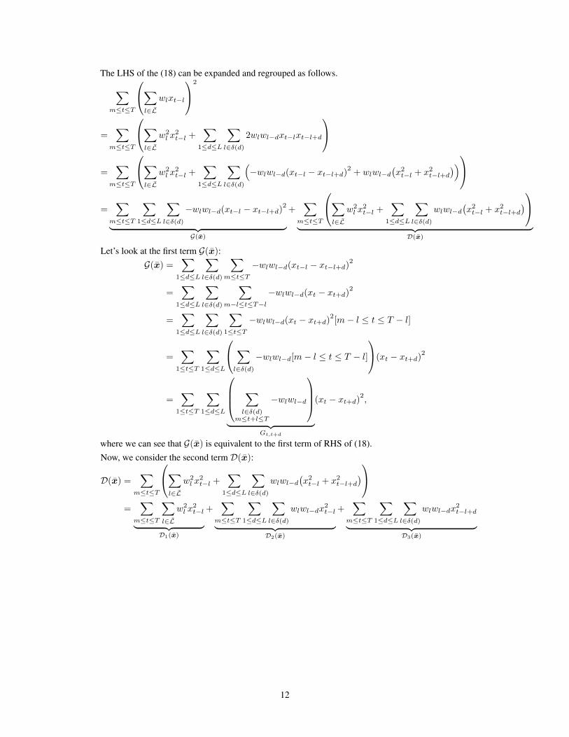
The LHS of the (18) can be expanded and regrouped as follows.∑m≤t≤T
∑l∈L
wlxt−l
2
=∑
m≤t≤T
∑l∈L
w2l x
2t−l +
∑1≤d≤L
∑l∈δ(d)
2wlwl−dxt−lxt−l+d
=
∑m≤t≤T
∑l∈L
w2l x
2t−l +
∑1≤d≤L
∑l∈δ(d)
(−wlwl−d(xt−l − xt−l+d)2
+ wlwl−d(x2t−l + x2
t−l+d))
=∑
m≤t≤T
∑1≤d≤L
∑l∈δ(d)
−wlwl−d(xt−l − xt−l+d)2
︸ ︷︷ ︸G(x)
+∑
m≤t≤T
∑l∈L
w2l x
2t−l +
∑1≤d≤L
∑l∈δ(d)
wlwl−d(x2t−l + x2
t−l+d)
︸ ︷︷ ︸D(x)
Let’s look at the first term G(x):G(x) =
∑1≤d≤L
∑l∈δ(d)
∑m≤t≤T
−wlwl−d(xt−l − xt−l+d)2
=∑
1≤d≤L
∑l∈δ(d)
∑m−l≤t≤T−l
−wlwl−d(xt − xt+d)2
=∑
1≤d≤L
∑l∈δ(d)
∑1≤t≤T
−wlwl−d(xt − xt+d)2[m− l ≤ t ≤ T − l]
=∑
1≤t≤T
∑1≤d≤L
∑l∈δ(d)
−wlwl−d[m− l ≤ t ≤ T − l]
(xt − xt+d)2
=∑
1≤t≤T
∑1≤d≤L
∑l∈δ(d)
m≤t+l≤T
−wlwl−d
︸ ︷︷ ︸
Gt,t+d
(xt − xt+d)2,
where we can see that G(x) is equivalent to the first term of RHS of (18).Now, we consider the second term D(x):
D(x) =∑
m≤t≤T
∑l∈L
w2l x
2t−l +
∑1≤d≤L
∑l∈δ(d)
wlwl−d(x2t−l + x2
t−l+d)
=∑
m≤t≤T
∑l∈L
w2l x
2t−l︸ ︷︷ ︸
D1(x)
+∑
m≤t≤T
∑1≤d≤L
∑l∈δ(d)
wlwl−dx2t−l︸ ︷︷ ︸
D2(x)
+∑
m≤t≤T
∑1≤d≤L
∑l∈δ(d)
wlwl−dx2t−l+d︸ ︷︷ ︸
D3(x)
12
D1(x) =∑l∈L
∑m≤t≤T
w2l x
2t−l =
∑l∈L
∑m−l≤t≤T−l
w2l x
2t =
∑1≤t≤T
∑l∈L
w2l [m ≤ t+ l ≤ T ]
x2t
=∑
1≤t≤T
∑l,l′∈L
wlwl′ [m ≤ t+ l ≤ T ][l′ = l]
x2t
D2(x) =∑
m≤t≤T
∑1≤d≤L
∑l∈δ(d)
wlwl−dx2t−l =
∑1≤t≤T
∑1≤d≤L
∑l∈δ(d)
wlwl−d[m ≤ t+ l ≤ T ]
x2t
=∑
1≤t≤T
∑l,l′∈L
wlwl′ [m ≤ t+ l ≤ T ][l′ < l]
x2t
D3(x) =∑
m≤t≤T
∑1≤d≤L
∑l∈δ(d)
wlwl−dx2t−l+d =
∑1≤t≤T
∑1≤d≤L
∑l∈δ(d)
wlwl−d[m ≤ t+ l − d ≤ T ]
x2t
=∑
1≤t≤T
∑l′,l∈L
wlwl′ [m ≤ t+ l ≤ T ][l′ > l]
x2t
Let D ∈ RT×T be a diagonal matrix with Dtt be the coefficient associated with x2t in D(x).
Combining the results of D1(x),D2(x), and D3(x), Dt can be written as follows.
Dtt =
∑l∈L
wl
∑l∈L
wl[m ≤ t+ l ≤ T ]
∀t.
It is clear that D(x) = x>Dx. Note that ∀t = m, . . . , T − L, Dtt =(∑
l∈L wl)2
.
C.2 Proof of Corollary 1Proof. It is well known that graph regularization can be written in the quadratic form [18] as follows.
1
2
∑t∼s
Gts(xt − xs)2= x> Lap(G)x,
where Lap(G) is the T × T graph Laplacian for G defined as:
Lap(G)ts =
∑j Gtj , t = s
−Gts, t 6= s and there is an edge t ∼ s0, otherwise.
Based on the above fact and the results from Theorem 1, we obtain the quadratic form forTAR(x |L, w, η) as follows.
TAR(x |L, w, η) =1
2x>
Lap(GAR)+D + ηI︸ ︷︷ ︸
diagonal
x.Because D+ ηI is diagonal, the non-zero pattern of the off-diagonal entries of the inverse covarianceΣ−1
AR for TAR(x |L, w, η) is determined by Lap(GAR
)which shares the same non-zero pattern as
GAR.
C.3 Details for Corollary 2We use results developed in [15] to arrive at our result. Assume we are given the matrix B. We firstdefine the following quantities:
α :=√nT‖Z?B‖∞‖Z?B‖F
β :=‖Z?B‖∗‖Z?B‖F
(19)
where the ‖ · ‖∞ norm is taken element-wise. Note that, the above quantities capture the “simplicity”of the matrix Z. For example, a small value of α implies that the matrix ZB is not overly spiky,
13
meaning that the entries of the matrix are well spread out in magnitude. Next, define the set
C :=
Z : αβ ≤ C
√N
log(n+ T )
, (20)
with C being a constant that depends on α.Finally, we assume the following observation model: for each i, j ∈ Ω, suppose we observe
Yij = Z?ij +σ√nT
ηij ηij ∼ N (0, 1)
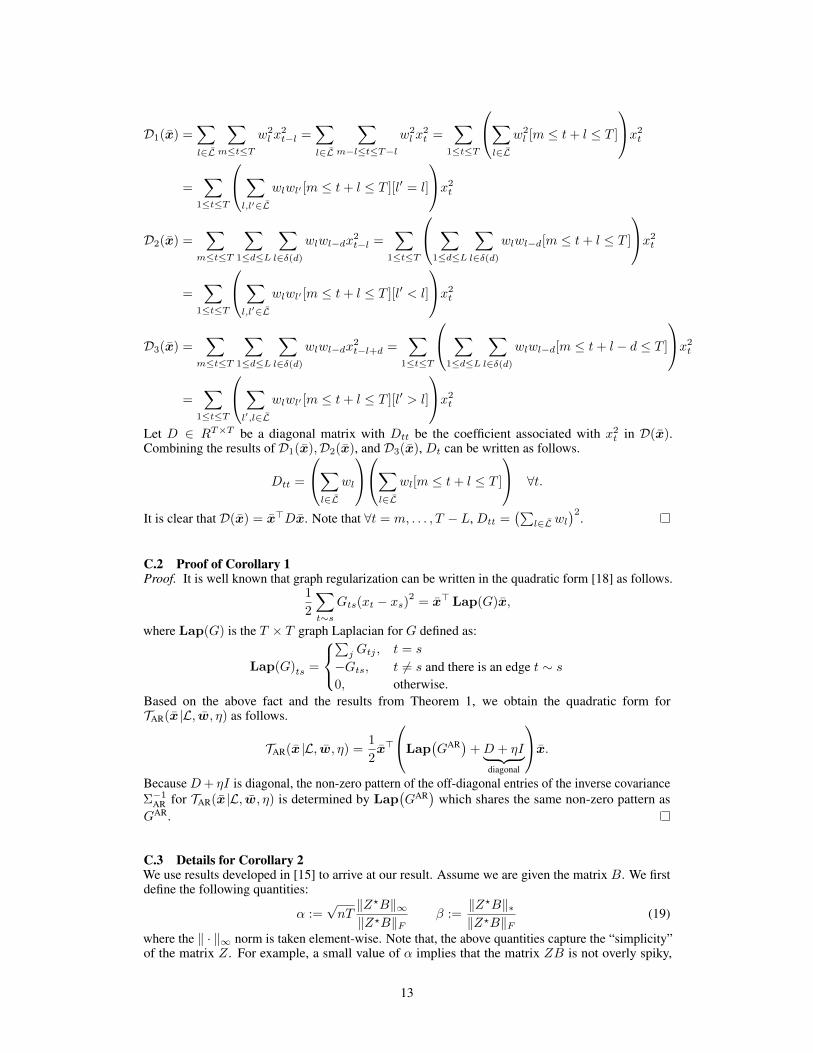
Then, we can see that the setup is identical to that considered in [15] with the difference being thatthere is no graph present that relates the rows of Z?. Hence, setting A = I in Theorem 1 in theaforementioned paper yields our result.
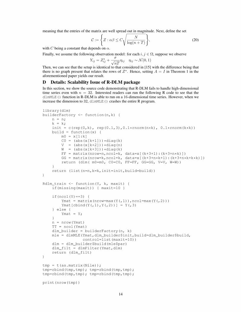
D Details: Scalability Issue of R-DLM packageIn this section, we show the source code demonstrating that R-DLM fails to handle high-dimensionaltime series even with n = 32. Interested readers can run the following R code to see that thedlmMLE() function in R-DLM is able to run on a 16-dimensional time series. However, when weincrease the dimension to 32, dlmMLE() crashes the entire R program.
library(dlm)builderFactory <- function(n,k)
n = n;k = k;init = c(rep(0,k), rep(0.1,3),0.1*rnorm(n*k), 0.1*rnorm(k*k))build = function(x)
m0 = x[1:k]C0 = (abs(x[k+1]))*diag(k)V = (abs(x[k+2]))*diag(n)W = (abs(x[k+3]))*diag(k)FF = matrix(nrow=n,ncol=k, data=x[(k+3+1):(k+3+n*k)])GG = matrix(nrow=k,ncol=k, data=x[(k+3+n*k+1):(k+3+n*k+k*k)])return (dlm( m0=m0, C0=C0, FF=FF, GG=GG, V=V, W=W))
return (list(n=n,k=k,init=init,build=build))
Rdlm_train <- function(Y, k, maxit) if(missing(maxit)) maxit=10
if(ncol(Y)==3) Ymat = matrix(nrow=max(Y(,1)),ncol=max(Y(,2)))Ymat[cbind(Y(,1),Y(,2))] = Y(,3)
else Ymat = Y;
n = nrow(Ymat)TT = ncol(Ymat)dlm_builder = builderFactory(n, k)mle = dlmMLE(Ymat,dlm_builder$init,build=dlm_builder$build,
control=list(maxit=10))dlm = dlm_builder$build(mle$par)dlm_filt = dlmFilter(Ymat,dlm)return (dlm_filt)
tmp = t(as.matrix(Nile));tmp=rbind(tmp,tmp); tmp=rbind(tmp,tmp);tmp=rbind(tmp,tmp); tmp=rbind(tmp,tmp);
print(nrow(tmp))
14
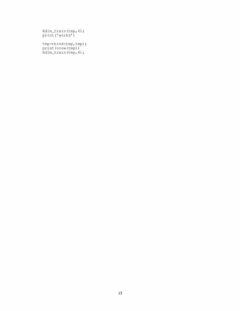
Rdlm_train(tmp,4);print(’works’)
tmp=rbind(tmp,tmp);print(nrow(tmp))Rdlm_train(tmp,4);
15