Embed Size (px)
Citation preview
Temporary threshold shift (TTS) in odontocetes in response to multiple air gun impulses Final Report James J. Finneran1, Carolyn E. Schlundt2, Brian K. Branstetter3, Jennifer S. Trickey4, Victoria Bowman3, and Keith Jenkins1 1 US Navy Marine Mammal Program, SSC Pacific, Code 2351, 53560 Hull St., San Diego, CA 92152 2 Exelis Inc. 3 National Marine Mammal Foundation 4 G2 Software Systems !
2
I. Executive Summary
To investigate the auditory effects of multiple underwater impulses, auditory thresholds were
measured in bottlenose dolphins before and after exposure to a series of impulses produced by a
seismic air gun. The pre- and post-exposure hearing thresholds were compared to determine the
amount of temporary hearing loss, called a temporary threshold shift (TTS), as a function of
exposure conditions.
Three dolphins (BLU, TYH, and OLY) participated in the study. Initial exposures for each
subject were designed to acclimate the dolphins to the sequence of underwater impulses and
featured between 2 and 5 impulses. This initial test phase ranged from several months (BLU,
TYH) to approximately 1 week (OLY), after which the primary data collection (Phase 1 testing)
began. During this phase, subjects were exposed to a sequence of 10 impulses, delivered at a rate
of one impulse every 10 seconds. Before and after each exposure sequence, thresholds were
measured at several frequencies using psychophysical (behavioral) and/or electrophysiological
[auditory evoked potential (AEP)] methods and compared to their pre-exposure values to
determine the amount of TTS induced. After no substantial differences were seen between the
post- and pre-exposure thresholds, the exposure level was increased (the dolphin was moved
incrementally closer, and/or the air gun pressure/volume were increased) on the next exposure
day and the process repeated.
During Phase 1, the dolphin BLU participated in a total of 46 exposure sessions and 45 control
sessions; TYH participated in 57 exposure sessions and 125 control sessions; and OLY
participated in 45 exposure and 122 control sessions. The maximum exposure for all three
subjects was 10 impulses, at a distance of 3.9 m from the air gun operating at 2000 psi with a
volume of 150 in3 (the maximum output configuration for the air gun with the dolphin at the
shortest practical distance). The mean cumulative sound exposure level (SEL) for the 150 in3,
2000 psi, and 3.9 m exposure conditions was 195, 194, and 189 dB re 1 µPa2s (for 10 impulses),
for BLU, TYH, and OLY, respectively.
No substantial TTS was observed in any subject, at any test frequency, for any combinations of
range, volume, or pressure during psychophysical testing. The electrophysiological measurements
were inconclusive. No measurable TTS was seen in BLU or OLY; however, TYH’s
electrophysiological data did show a small TTS after exposure to 10 impulses from the air gun at
the 150 in3, 1500 psi, and 3.9 m range condition (193 dB re 1 µPa2s cumulative SEL). Exposure
at a higher level produced a smaller TTS, and later testing using tone-pip stimuli failed to produce
3
any TTS. It is not known to what extent TYH’s “anticipatory” behavior during the highest
exposures (see below) affected the TTS results (i.e., whether he was able to mitigate the effects of
the exposure).
The results of this study contrast with previous TTS testing with a seismic watergun, where
(behavioral) TTS was observed in a beluga after an exposure with SEL of 186 dB re 1 µPa2s. The
differences between the auditory and behavioral effects of the watergun and air gun may have
been a result of the relatively low frequency content of air gun impulses compared to the
relatively high-frequency hearing ability of dolphins, or the lower peak-peak pressures produced
by the air gun.
No behavioral reactions were observed in BLU after exposure to the air gun impulses. Behavioral
reactions were observed in both TYH and OLY after exposure to the air gun impulses at the
maximum output level. Both subjects appeared to anticipate the next exposure in a sequence and
may have been attempting to mitigate the effects of the impulses.
After the Phase 1 testing, follow-on testing was conducted with OLY and TYH to explore the use
of alternate evoked potential methods and to further examine the anticipatory behavioral
reactions. During these tests, no substantial differences were seen in the AEP data when using
tone-pip stimuli compared to the sinusoidal amplitude modulated tone stimuli used previously. In
OLY, evoked potential data collected in response to an external sound stimulus presented during
the air gun exposures showed a temporal correlation with the air gun impulses — the AEP
amplitude followed a cyclical pattern of decreasing after each impulse. This pattern of decreasing
hearing sensitivity is believed to have been a result of either the middle ear reflex, a short-term
TTS, or active self-mitigation of the air gun noise exposure by the dolphin.
4
II. Background
It is becoming increasingly clear that intense anthropogenic (human-generated) underwater sound
may adversely affect the hearing and behavior of many marine mammals, including dolphins and
whales. Unfortunately, there are few data regarding the effects of intense sound on these
mammals, making it difficult to predict safe exposure levels.
Exposure to intense sound may produce an elevated hearing threshold, also known as a noise-
induced threshold shift. If the threshold returns to the pre-exposure level after a period of time,
the threshold shift is known as a temporary threshold shift (TTS); if the threshold does not return
to the pre-exposure level, the threshold shift is called a permanent threshold shift (PTS). PTS
results in damage to the auditory system and sensory hair cell loss. Moderate, occasional TTS is
fully reversible and does not result in permanent injury; TTS may thus be used to estimate safe
limits of exposure to avoid PTS.
Studies of PTS and TTS in terrestrial mammals were instrumental in establishing noise exposure
limits in humans; however, there are no PTS data and few TTS data for marine mammals. The
majority of existing marine mammal TTS data concern the effects of single, continuous exposures
to steady-state signals such as tones (e.g., Finneran et al., 2010a; Finneran et al., 2005; Finneran
et al., 2007; Ridgway et al., 1997; Schlundt et al., 2000) or broadband noise (e.g., {Nachtigall,
2003 #2266;Nachtigall, 2004 #13379;Kastak, 1999 #1703;Kastak, 2005 #3559;Popov, 2011
#24096;Mooney, 2009 #21748; Popov, 2013 #28013; Kastelein, 2012 #28015; Kastelein, 2012
#28016}). Although pure tones may approximate many military and commercial sonars and
broadband noise allows comparison with existing terrestrial data obtained under similar
conditions, many anthropogenic sources of intense sound produce impulsive signals, i.e. transient
signals with rapid rise times and high peak pressures. Impulsive sources include impact pile
driving, underwater explosions, and seismic air guns. TTS data obtained with broadband noise or
tones may suggest the effects of impulsive sounds; however, the relationship between hearing
loss and the fundamental parameters of sound such as peak frequency, duration, rise time, peak
pressure, and total energy are unknown, thus TTS measurements with impulsive stimuli are
needed for direct predictions. Limited data exist regarding marine mammals exposed to impulsive
sounds produced by an “explosion simulator” (Finneran et al., 2000), a seismic watergun
(Finneran et al., 2002), an arc-gap transducer (Finneran et al., 2003), and a seismic air gun (Lucke
et al., 2009). All of these studies featured exposures consisting of single impulses only; there are
no TTS data for marine mammals exposed to multiple impulses.
5
III. Objectives of this study
The objectives of this study were to measure the amount of TTS induced in trained bottlenose
dolphins (Tursiops truncatus) after exposure to multiple impulses produced by a seismic air gun.
Two test phases were planned: (1) Determine the most susceptible frequency to TTS after
exposure to 10 air gun impulses, and (2) determine the relationship between TTS, the received
sound pressure level (SPL), and the number of impulses.
During Phase 1 testing no substantial effects were observed after exposure to 10 impulses at the
highest exposure levels, therefore, Phase 2 testing was not performed. Instead, follow-on testing
was conducted to examine different evoked potential measurement approaches and the behavioral
reactions exhibited by the subjects.
IV. Subjects and test environment
Three Atlantic bottlenose dolphins participated in the experiments: BLU (female, approximately
45–46 y at the time of testing, ~200 kg), TYH (male, 30–32 y, 200 kg), and OLY (male, 27–29 y,
200 kg). All three animals had experience with cooperative psychophysical testing, and BLU and
TYH previously participated in TTS experiments (Finneran et al., 2010a; b; Finneran and
Schlundt, 2010; Finneran et al., 2007). During the course of the study, BLU became pregnant
and, as a result, her participation ended somewhat sooner than originally planned.
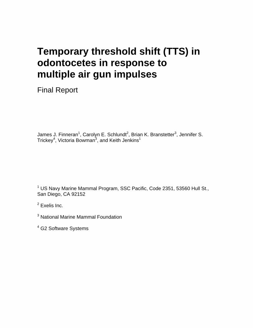
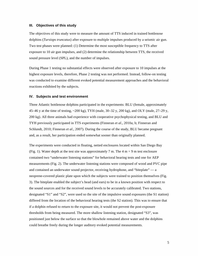
The experiments were conducted in floating, netted enclosures located within San Diego Bay
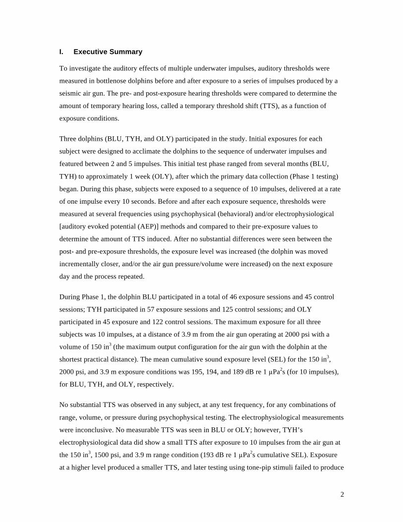
(Fig. 1). Water depth at the test site was approximately 7 m. The 4 m × 9 m test enclosure
contained two “underwater listening stations” for behavioral hearing tests and one for AEP
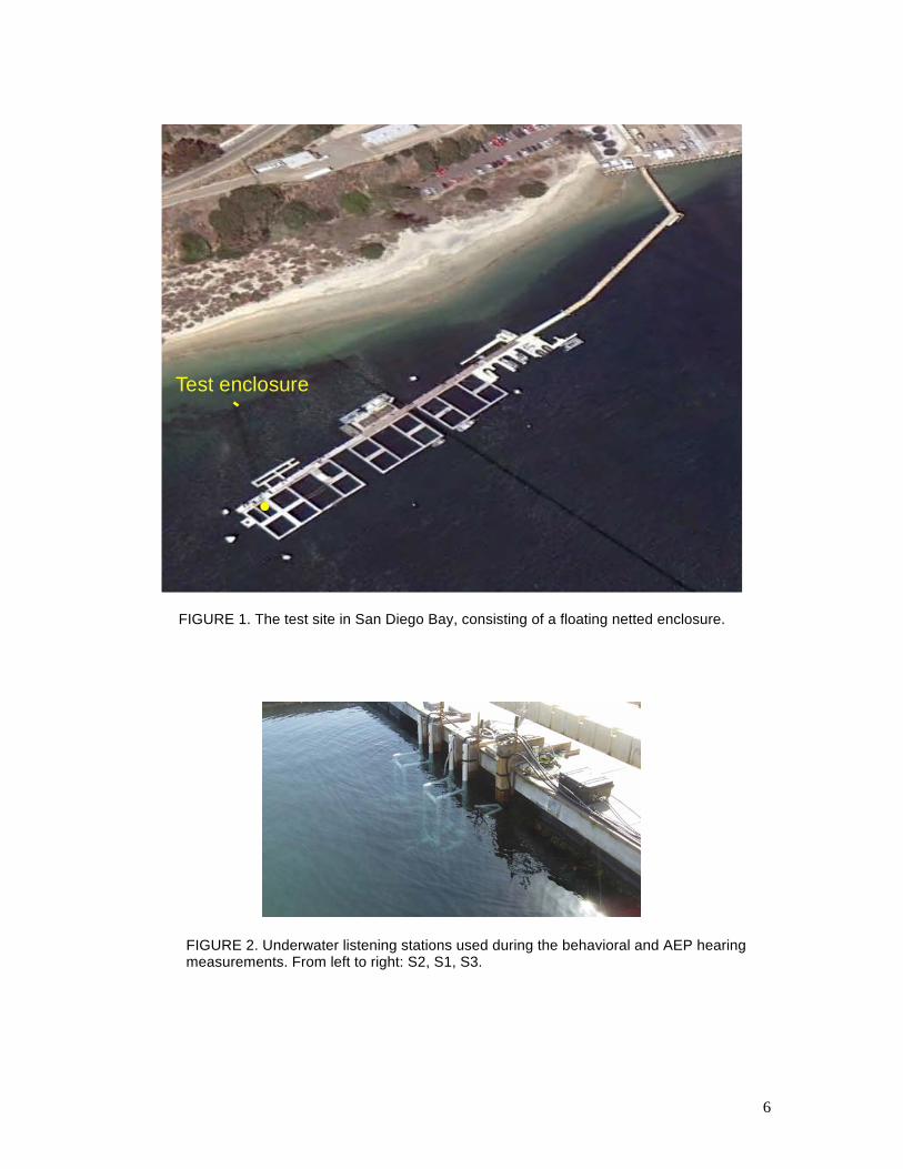
measurements (Fig. 2). The underwater listening stations were composed of wood and PVC pipe
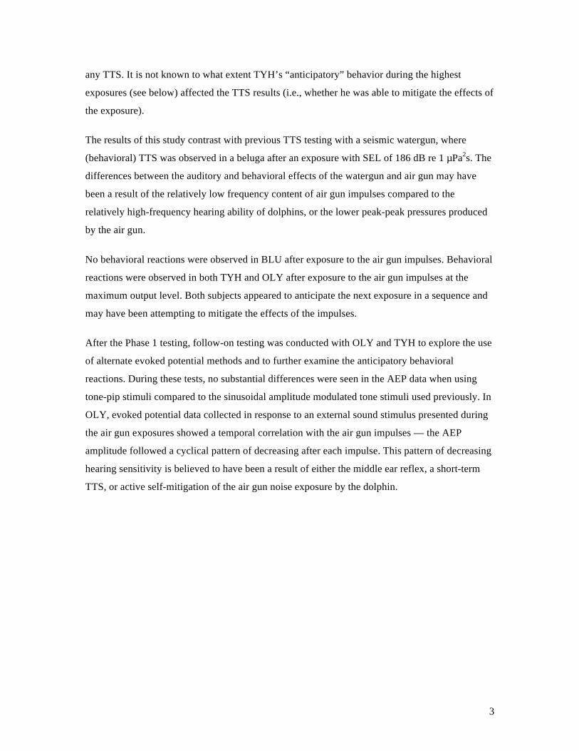
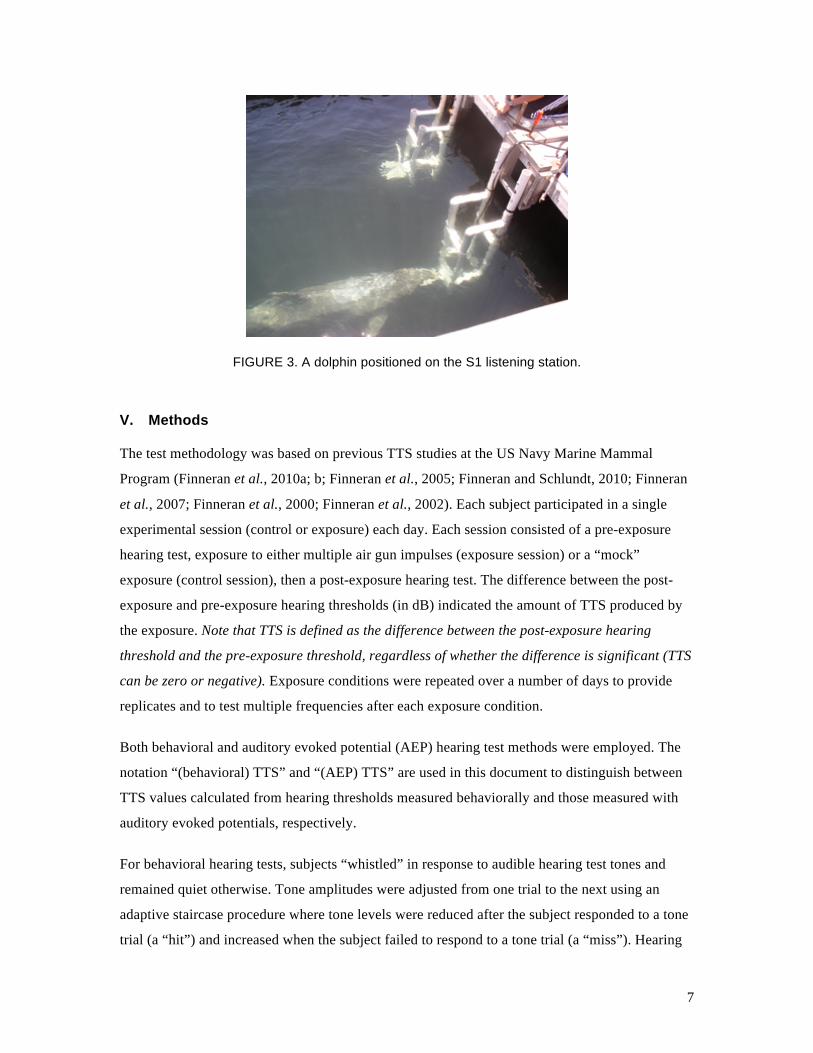
and contained an underwater sound projector, receiving hydrophone, and “biteplate” — a
neoprene-covered plastic plate upon which the subjects were trained to position themselves (Fig.
3). The biteplate enabled the subject’s head (and ears) to be in a known position with respect to
the sound sources and for the received sound levels to be accurately calibrated. Two stations,
designated “S1” and “S2”, were used so the site of the impulsive sound exposures (the S1 station)
differed from the location of the behavioral hearing tests (the S2 station). This was to ensure that
if a dolphin refused to return to the exposure site, it would not prevent the post-exposure
thresholds from being measured. The more shallow listening station, designated “S3”, was
positioned just below the surface so that the blowhole remained above water and the dolphins
could breathe freely during the longer auditory evoked potential measurements.
6
FIGURE 1. The test site in San Diego Bay, consisting of a floating netted enclosure.
FIGURE 2. Underwater listening stations used during the behavioral and AEP hearing measurements. From left to right: S2, S1, S3.
Test enclosure
7
FIGURE 3. A dolphin positioned on the S1 listening station.
V. Methods
The test methodology was based on previous TTS studies at the US Navy Marine Mammal
Program (Finneran et al., 2010a; b; Finneran et al., 2005; Finneran and Schlundt, 2010; Finneran
et al., 2007; Finneran et al., 2000; Finneran et al., 2002). Each subject participated in a single
experimental session (control or exposure) each day. Each session consisted of a pre-exposure
hearing test, exposure to either multiple air gun impulses (exposure session) or a “mock”
exposure (control session), then a post-exposure hearing test. The difference between the post-
exposure and pre-exposure hearing thresholds (in dB) indicated the amount of TTS produced by
the exposure. Note that TTS is defined as the difference between the post-exposure hearing
threshold and the pre-exposure threshold, regardless of whether the difference is significant (TTS
can be zero or negative). Exposure conditions were repeated over a number of days to provide
replicates and to test multiple frequencies after each exposure condition.
Both behavioral and auditory evoked potential (AEP) hearing test methods were employed. The
notation “(behavioral) TTS” and “(AEP) TTS” are used in this document to distinguish between
TTS values calculated from hearing thresholds measured behaviorally and those measured with
auditory evoked potentials, respectively.
For behavioral hearing tests, subjects “whistled” in response to audible hearing test tones and
remained quiet otherwise. Tone amplitudes were adjusted from one trial to the next using an
adaptive staircase procedure where tone levels were reduced after the subject responded to a tone
trial (a “hit”) and increased when the subject failed to respond to a tone trial (a “miss”). Hearing
8
thresholds were based on the average tone level of at least five hit-miss or miss-hit reversal points
and could generally be estimated within 2–4 min per frequency tested. Up to three behavioral test
frequencies were tested immediately before and immediately after the exposures (or mock
exposures) in each session. When more than one frequency was tested, the frequencies were
presented to the subject in reverse order in the pre- and post-exposure sessions so that the
frequency tested immediately before the exposure was also tested immediately after the exposure.
AEP hearing tests utilized the single (TYH and OLY) and multiple (BLU) auditory steady state
response technique (ASSR; Finneran et al., 2007), where sinusoidal amplitude modulated (SAM)
tones were presented using a descending method of limits and the evoked responses at the
modulation rates tracked to estimate thresholds at individual tone frequencies. AEPs were
typically measured before and after the behavioral tests which surrounded the exposures (or mock
exposures). The multiple ASSR method allowed hearing to be simultaneously tested at four
frequencies simultaneously. Two frequencies were normally tested when the single ASSR
technique was employed. As with the behavioral frequencies, AEP test frequencies were
presented in reverse order before and after the (mock) exposures. The ASSR approach does not
work particularly well at low frequencies (below ~ 8 kHz) and is less precise compared to the
behavioral approach.
Because the subjects’ reactions to the exposures were unknown, they were trained to wear a self-
contained hydrophone dosimeter (BLU) or cabled hydrophones attached to suction cups (TYH
and OLY) during the impulsive sound exposures. This allowed estimates of the received sound
levels regardless of the subject’s location within the test enclosure.
VI. Accomplishments
1. Environmental Assessment
This project was performed via a Cooperative Research and Development Agreement (CRADA)
between the US Navy and the International Association of Oil and Gas Producers (OGP). The
CRADA specified that the seismic air gun could not be operated in San Diego Bay until the
requirements of the National Environmental Policy Act (NEPA) were met; i.e., until the potential
environmental effects of the project were analyzed. To satisfy the NEPA requirements, we
conducted an environmental impact analysis and prepared an Environmental Assessment (EA).
After reviewing the EA, a finding of ‘No Significant Impact’ was reached by the US Navy, Chief
of Naval Operations (N456).
9
2. Monitoring and mitigation
The EA specified that the air gun could be fired a maximum of three days per week, with a
maximum of 50 impulses per day. The EA also specified a monitoring plan and mitigation
measures (i.e., do not fire the air gun if protected animals are within specified safety zones) to
ensure that wild marine mammals and other protected species would not be not exposed to
harmful sound levels.
Over the course of the study, the air gun was fired on 215 separate days, with a total of 3,113
impulses generated. Occasionally, multiple efforts (< 50 impulses total) were conducted within a
single day. Mitigation measures were implemented on 73 of the 215 days, with a total of 79
mitigation actions. Twelve of the mitigation actions involved stopping the operation of the air gun
during an ongoing shot sequence or canceling an effort prior to shots being fired. The other 67
events involved delaying the operation of the air gun until the safety zones were clear, after which
operations continued. Thirty-three of the delayed mitigation actions involved other Navy
activities (e.g., pausing operation of the air gun until Navy divers or swimmers left the water).
The remaining 34 of the delayed mitigation actions involved pausing operation of the air gun
until protected wildlife left the safety zone. Fourteen of the 34 delayed mitigation actions were
the result of a specific harbor seal that repeatedly “hauled-out” on the floating enclosures near the
test site (within the safety range for harbor seals). There were no significant changes in behavior
noted in any protected wildlife during operations of the air gun.
3. Air gun output characterization
The air gun was a Sercel G-Gun 150, with an adjustable volume from 40 to 150 in3. The air gun
was deployed from a wench attached to a floating platform positioned in front of the S1 listening
station. The air gun was always deployed to a depth of 2 m and suspended from the front and rear
flanges so the long axis of the air gun was horizontal in the water column.
The air gun was pressured from a high-pressure air system, consisting of a compressor, storage
tanks, and various valves and regulators. The high-pressure system we received with the air gun
included a gasoline compressor and relatively small storage volume. Initial tests revealed that the
system could not supply enough air at a sufficient rate to fire 10 or more impulses at a 10-s
interval with an air gun volume of 150 in3 and pressure of 2000 psi. We therefore designed and
fabricated a new high-pressure air system (Fig. 4), which featured an electric compressor
operating at ~3000 psi and included four large “K-style” gas bottles with a storage volume of
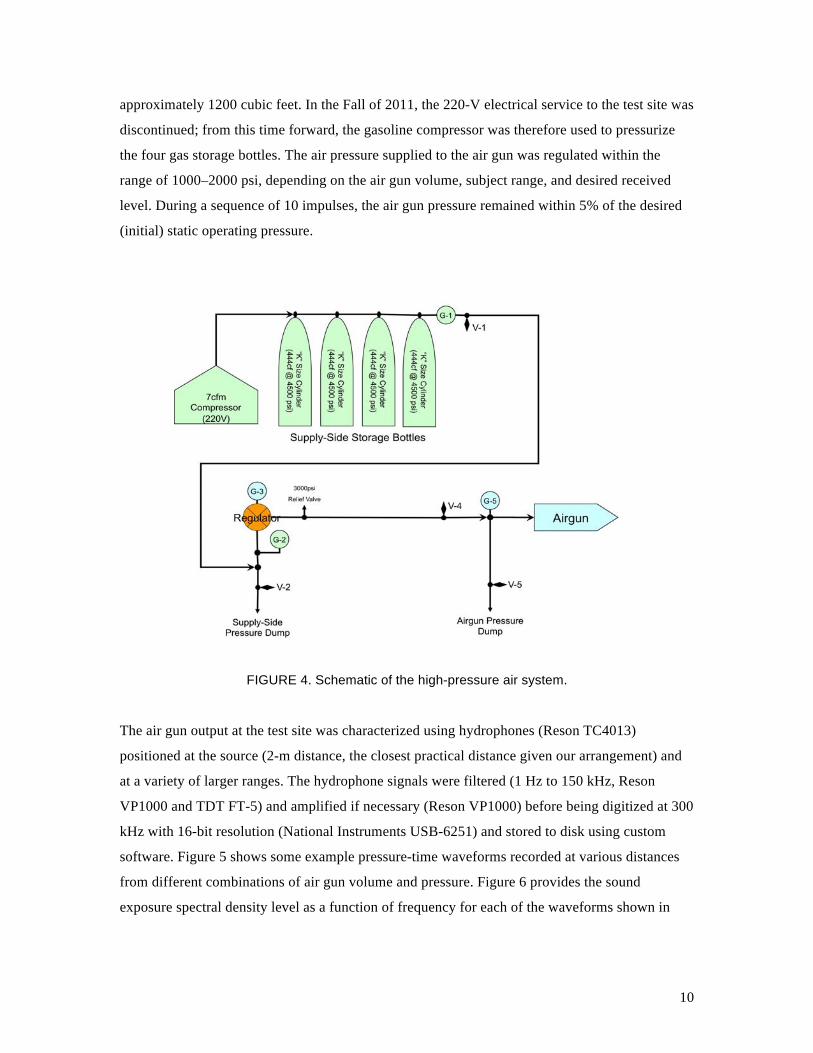
10
approximately 1200 cubic feet. In the Fall of 2011, the 220-V electrical service to the test site was
discontinued; from this time forward, the gasoline compressor was therefore used to pressurize
the four gas storage bottles. The air pressure supplied to the air gun was regulated within the
range of 1000–2000 psi, depending on the air gun volume, subject range, and desired received
level. During a sequence of 10 impulses, the air gun pressure remained within 5% of the desired
(initial) static operating pressure.
FIGURE 4. Schematic of the high-pressure air system.
The air gun output at the test site was characterized using hydrophones (Reson TC4013)
positioned at the source (2-m distance, the closest practical distance given our arrangement) and
at a variety of larger ranges. The hydrophone signals were filtered (1 Hz to 150 kHz, Reson
VP1000 and TDT FT-5) and amplified if necessary (Reson VP1000) before being digitized at 300
kHz with 16-bit resolution (National Instruments USB-6251) and stored to disk using custom
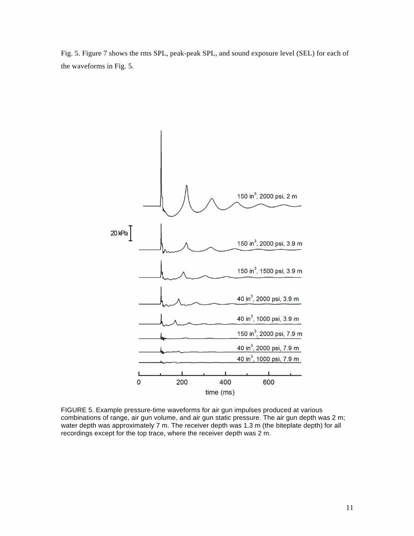
software. Figure 5 shows some example pressure-time waveforms recorded at various distances
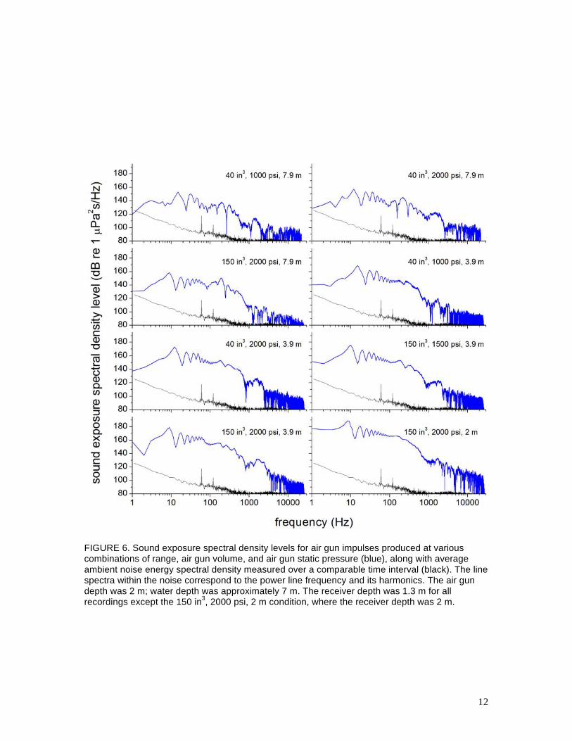
from different combinations of air gun volume and pressure. Figure 6 provides the sound
exposure spectral density level as a function of frequency for each of the waveforms shown in
11
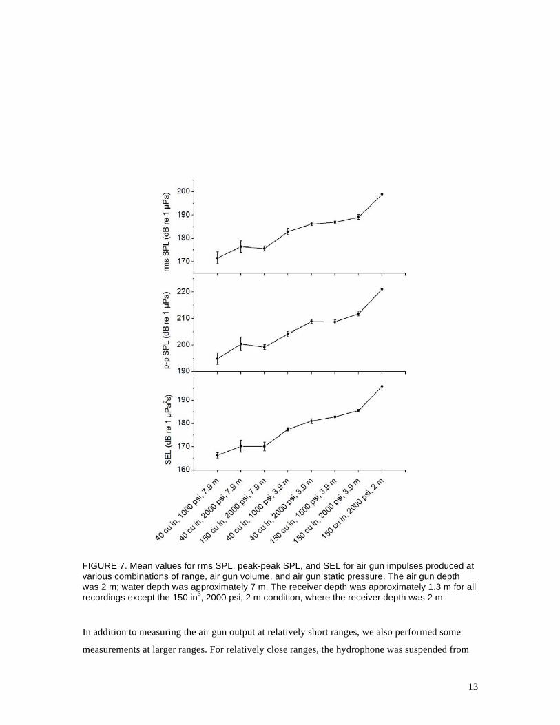
Fig. 5. Figure 7 shows the rms SPL, peak-peak SPL, and sound exposure level (SEL) for each of
the waveforms in Fig. 5.
FIGURE 5. Example pressure-time waveforms for air gun impulses produced at various combinations of range, air gun volume, and air gun static pressure. The air gun depth was 2 m; water depth was approximately 7 m. The receiver depth was 1.3 m (the biteplate depth) for all recordings except for the top trace, where the receiver depth was 2 m.
12
FIGURE 6. Sound exposure spectral density levels for air gun impulses produced at various combinations of range, air gun volume, and air gun static pressure (blue), along with average ambient noise energy spectral density measured over a comparable time interval (black). The line spectra within the noise correspond to the power line frequency and its harmonics. The air gun depth was 2 m; water depth was approximately 7 m. The receiver depth was 1.3 m for all recordings except the 150 in3, 2000 psi, 2 m condition, where the receiver depth was 2 m.
13
FIGURE 7. Mean values for rms SPL, peak-peak SPL, and SEL for air gun impulses produced at various combinations of range, air gun volume, and air gun static pressure. The air gun depth was 2 m; water depth was approximately 7 m. The receiver depth was approximately 1.3 m for all recordings except the 150 in3, 2000 psi, 2 m condition, where the receiver depth was 2 m.
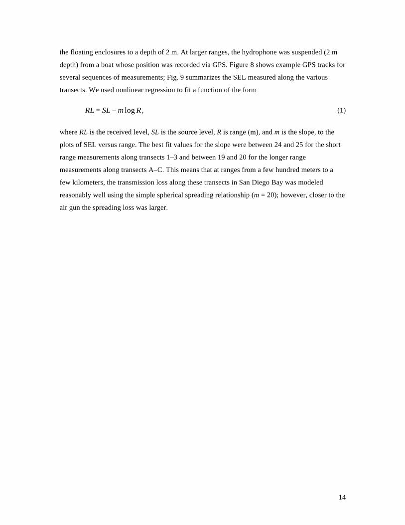
In addition to measuring the air gun output at relatively short ranges, we also performed some
measurements at larger ranges. For relatively close ranges, the hydrophone was suspended from
14
the floating enclosures to a depth of 2 m. At larger ranges, the hydrophone was suspended (2 m
depth) from a boat whose position was recorded via GPS. Figure 8 shows example GPS tracks for
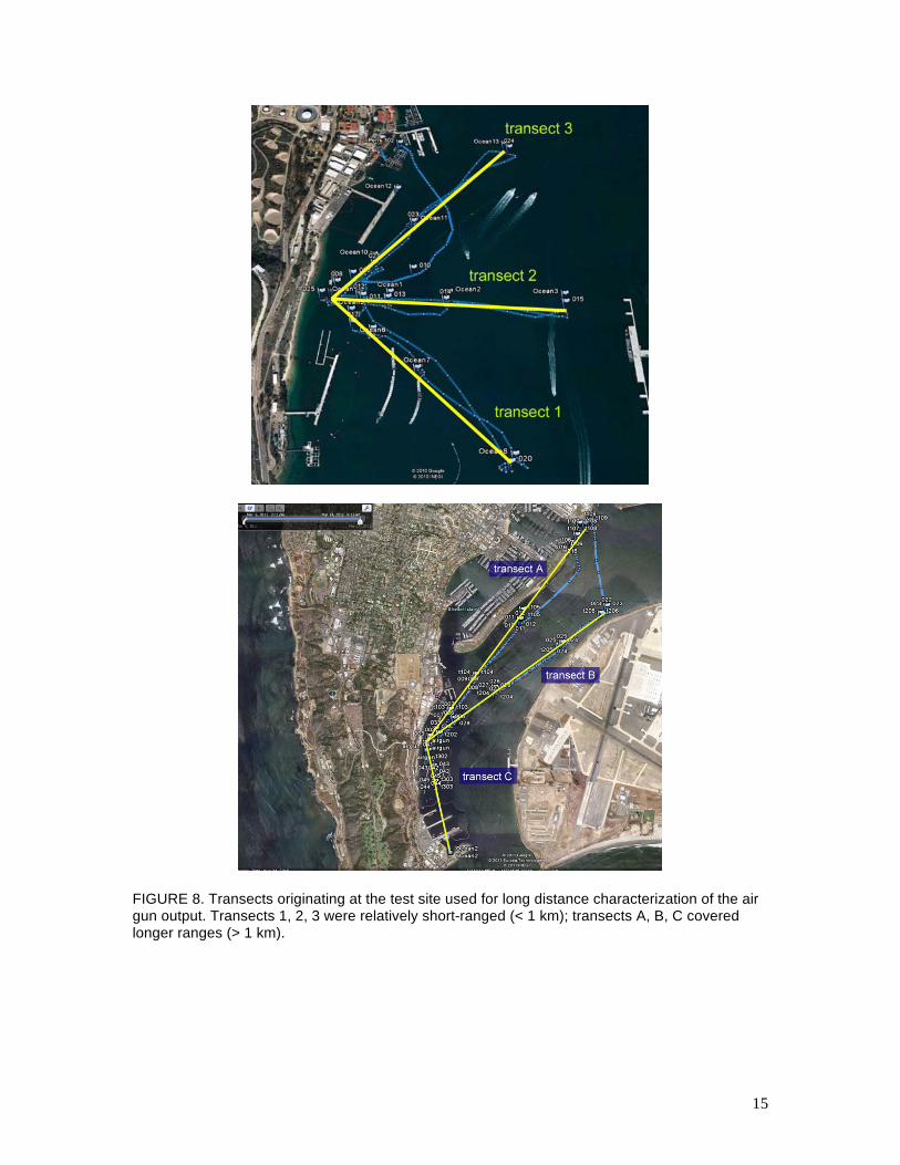
several sequences of measurements; Fig. 9 summarizes the SEL measured along the various
transects. We used nonlinear regression to fit a function of the form
€
RL = SL −m log R , (1)
where RL is the received level, SL is the source level, R is range (m), and m is the slope, to the
plots of SEL versus range. The best fit values for the slope were between 24 and 25 for the short
range measurements along transects 1–3 and between 19 and 20 for the longer range
measurements along transects A–C. This means that at ranges from a few hundred meters to a
few kilometers, the transmission loss along these transects in San Diego Bay was modeled
reasonably well using the simple spherical spreading relationship (m = 20); however, closer to the
air gun the spreading loss was larger.
15
FIGURE 8. Transects originating at the test site used for long distance characterization of the air gun output. Transects 1, 2, 3 were relatively short-ranged (< 1 km); transects A, B, C covered longer ranges (> 1 km).
16
FIGURE 9. SEL generated by the air gun (volume = 150 in3, static pressure = 2000 psi, depth = 2 m) along the transects shown in Fig. 8.
4. Baseline hearing thresholds
Although audiograms in a quiet pool existed for BLU and TYH, and OLY’s hearing ability was
known from previous AEP measurements, hearing thresholds had not been measured in San
Diego Bay at the test site, where the ambient noise levels were relatively high and variable (Fig.
10). We therefore measured baseline hearing thresholds for each subject, at the test site, using
behavioral techniques (the most accurate method). The frequency range for baseline hearing tests
17
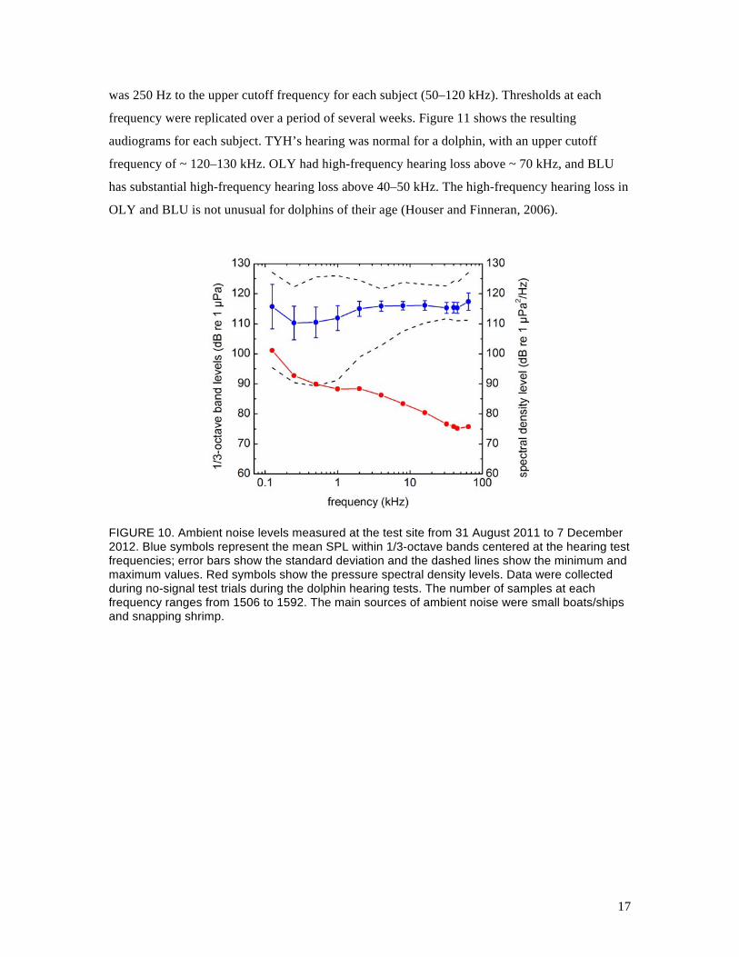
was 250 Hz to the upper cutoff frequency for each subject (50–120 kHz). Thresholds at each
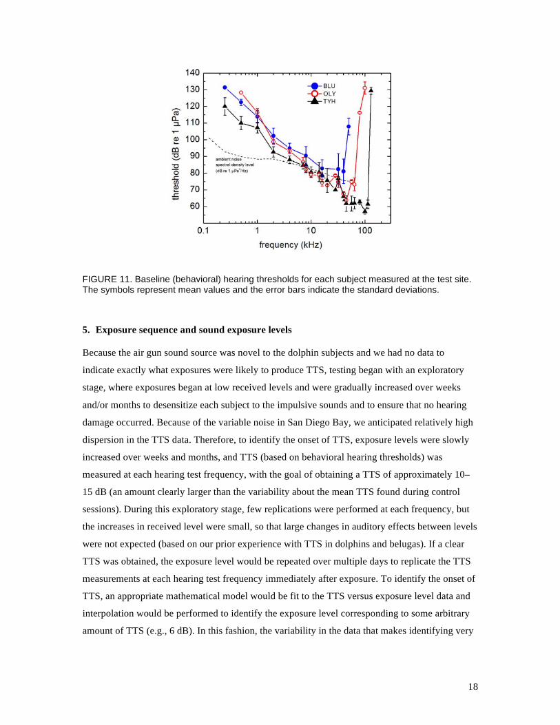
frequency were replicated over a period of several weeks. Figure 11 shows the resulting
audiograms for each subject. TYH’s hearing was normal for a dolphin, with an upper cutoff
frequency of ~ 120–130 kHz. OLY had high-frequency hearing loss above ~ 70 kHz, and BLU
has substantial high-frequency hearing loss above 40–50 kHz. The high-frequency hearing loss in
OLY and BLU is not unusual for dolphins of their age (Houser and Finneran, 2006).
FIGURE 10. Ambient noise levels measured at the test site from 31 August 2011 to 7 December 2012. Blue symbols represent the mean SPL within 1/3-octave bands centered at the hearing test frequencies; error bars show the standard deviation and the dashed lines show the minimum and maximum values. Red symbols show the pressure spectral density levels. Data were collected during no-signal test trials during the dolphin hearing tests. The number of samples at each frequency ranges from 1506 to 1592. The main sources of ambient noise were small boats/ships and snapping shrimp.
18
FIGURE 11. Baseline (behavioral) hearing thresholds for each subject measured at the test site. The symbols represent mean values and the error bars indicate the standard deviations.
5. Exposure sequence and sound exposure levels
Because the air gun sound source was novel to the dolphin subjects and we had no data to
indicate exactly what exposures were likely to produce TTS, testing began with an exploratory
stage, where exposures began at low received levels and were gradually increased over weeks
and/or months to desensitize each subject to the impulsive sounds and to ensure that no hearing
damage occurred. Because of the variable noise in San Diego Bay, we anticipated relatively high
dispersion in the TTS data. Therefore, to identify the onset of TTS, exposure levels were slowly
increased over weeks and months, and TTS (based on behavioral hearing thresholds) was
measured at each hearing test frequency, with the goal of obtaining a TTS of approximately 10–
15 dB (an amount clearly larger than the variability about the mean TTS found during control
sessions). During this exploratory stage, few replications were performed at each frequency, but
the increases in received level were small, so that large changes in auditory effects between levels
were not expected (based on our prior experience with TTS in dolphins and belugas). If a clear
TTS was obtained, the exposure level would be repeated over multiple days to replicate the TTS
measurements at each hearing test frequency immediately after exposure. To identify the onset of
TTS, an appropriate mathematical model would be fit to the TTS versus exposure level data and
interpolation would be performed to identify the exposure level corresponding to some arbitrary
amount of TTS (e.g., 6 dB). In this fashion, the variability in the data that makes identifying very
19
small amounts of TTS difficult would not prevent the identification of the exposure conditions
corresponding to the “onset” of TTS.
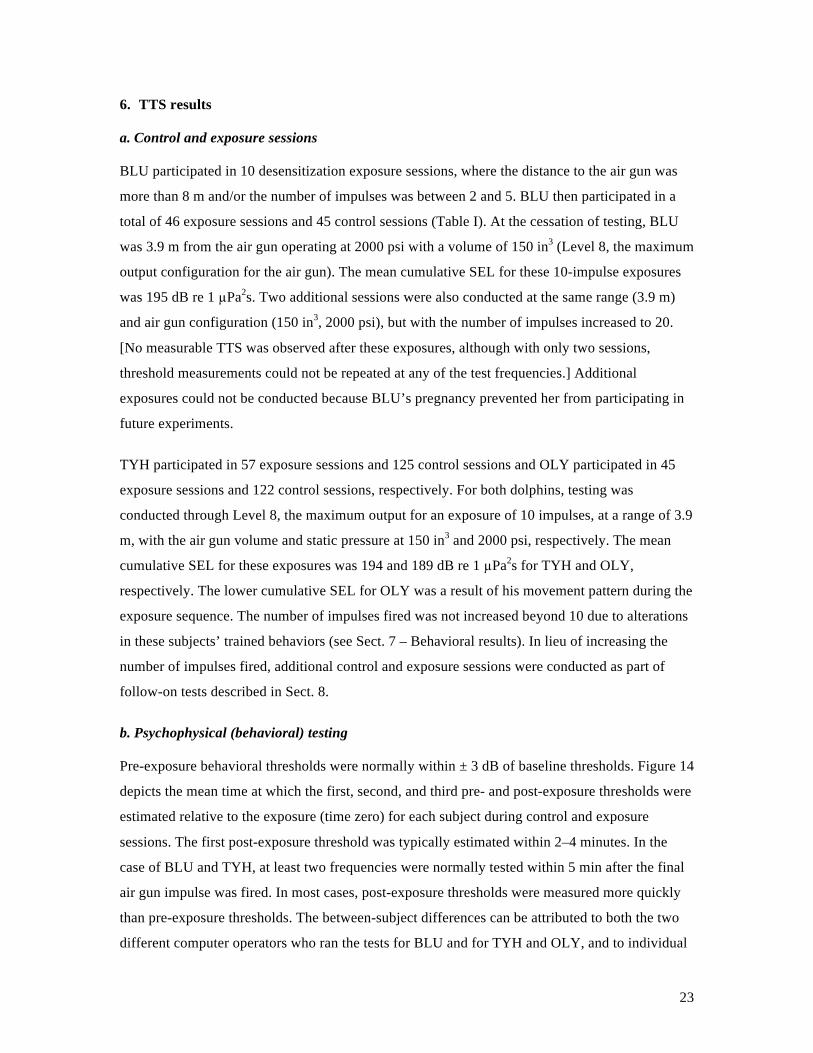
Eight different exposure “levels” — configurations of volume, pressure, and distance between the
air gun and the subject — were used during the study. Mean p-p SPLs, rms SPLs, and cumulative
SELs (for 10 impulses) for each of these configurations measured during the exposure sessions
for each subject are provided in Tables I—III.
At least one calibration impulse was fired before a subject arrived at the test site to ensure the air
gun was operational and that output levels remained consistent throughout the study. During
initial tests with BLU, calibration impulses were recorded by one Reson 4013 hydrophone placed
at the position of the midpoint between the subject’s ears when properly stationed underwater on
the S2 biteplate. Calibrations during the period of subsequent testing with TYH and OLY were
measured using two Reson 4013 hydrophones placed near the position of the subject’s ears when
stationed on the S1 biteplate. Calibration SELs measured between the two hydrophones were
normally within 1 dB of each other.
BLU was the first subject to participate in the study. Since the air gun effect on her hearing and
behavior was unknown, BLU was free swimming in an enclosure approximately 50 m from the
air gun, which was charged to 1000 psi with a volume of 40 in3, for her initial exposure. Over a
period of several weeks, BLU was moved closer to the air gun, the number of impulses increased,
and the air gun volume and pressure were increased. After each exposure sequence, behavioral
and AEP hearing thresholds were measured at several frequencies and compared to their pre-
exposure values. After no substantial differences were observed between the post- and pre-
exposure thresholds, the exposure level was increased (BLU was moved incrementally closer,
and/or the air gun pressure/volume were increased) on the next exposure day and the process
repeated. Exposure sessions with the dolphins TYH and OLY began after BLU was finished,
therefore we were able to use the results obtained with BLU to develop a reduced exposure
sequence for use with TYH and OLY (see Tables II and III). Again, exposures began at relatively
low received levels and incrementally increased as no TTS was observed.
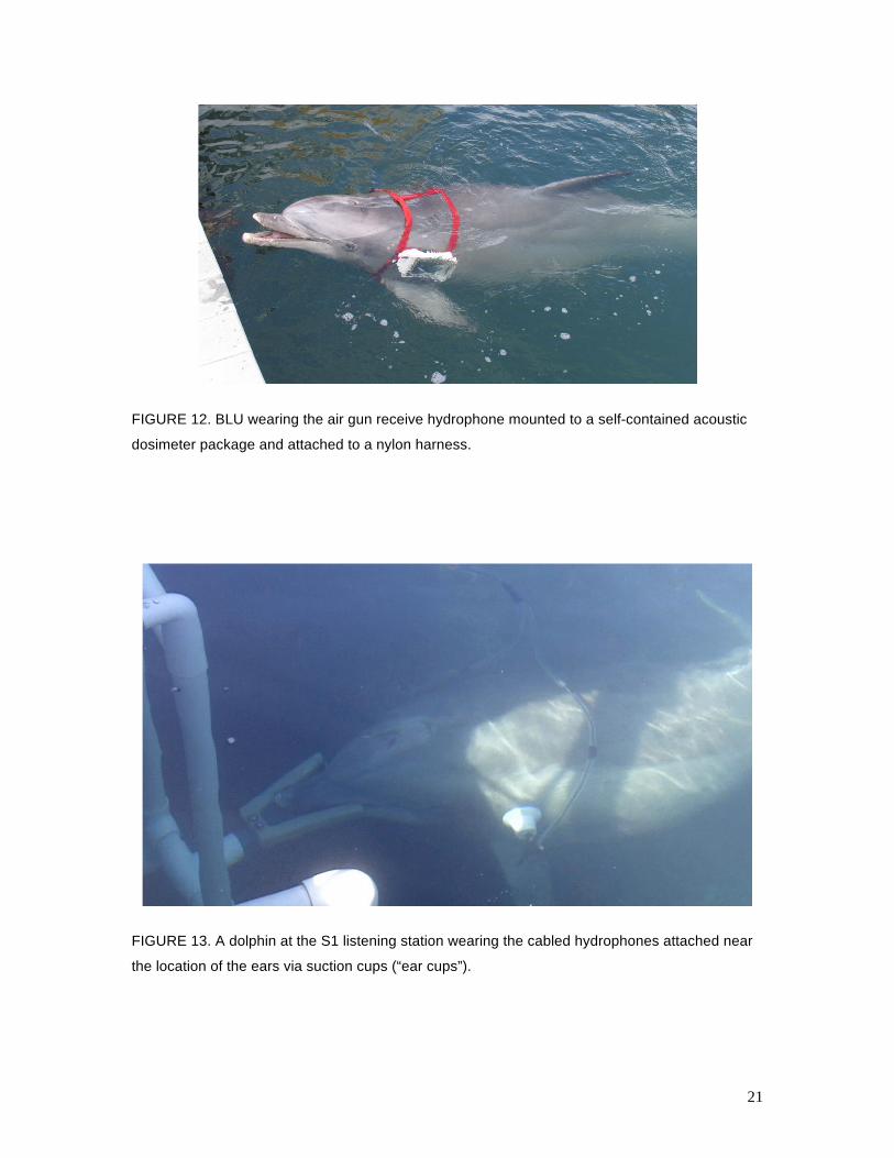
Exposure levels for BLU presented in Table I were measured by a single Reson 4013 hydrophone
mounted to a self-contained acoustic dosimeter package and attached to a nylon harness which
BLU wore during the control and exposure sessions (Fig. 12). Because we initially believed the
animals might show aversive behavior and swim about the enclosure during the exposures, the
20
dosimeter package allowed BLU to swim freely and record impulses regardless of her position in
the test enclosure.
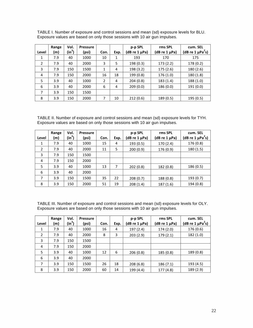
To measure the received levels during TYH and OLY’s exposure sessions, we replaced the
dosimeter with cabled hydrophones attached via suction cups near the location of the ears (Fig.
13). This allowed a more accurate measurement of the exposure levels using higher sampling
rates. The cabled hydrophones were used in both control and exposure sessions, and allowed
impulses to be recorded regardless of the subject’s location in the test enclosure. TYH had
previous experience wearing the cabled hydrophones and wore them throughout the study. OLY
did not begin wearing the hydrophones until testing at Level 7; during Levels 1, 2 and 5, the
hydrophones were placed near the calibration position on the S1 station and did not move during
the exposure even if OLY may have. Custom software allowed for real-time measurement of
individual impulses received at each ear (or at the S1 station). On occasion, one channel of the
hydrophone inputs experienced a faulty/noisy connection and those data were dropped from
analysis. Similarly, measurements that occurred when a hydrophone was out-of-water due to the
animal’s movement around the test enclosure during the exposure were discarded as well (see
Sect. 7 – Behavioral Results). If poor data quality prevented analyzing both hydrophone signals
for a particular impulse, the SEL for that particular impulse was estimated using the mean SEL
from the other impulses within the sequence. At the higher exposure levels, there was much more
variation in the received levels for TYH and OLY when behavioral reactions to the exposures
were observed (see Sect. 7 – Behavioral reactions).
21
FIGURE 12. BLU wearing the air gun receive hydrophone mounted to a self-contained acoustic
dosimeter package and attached to a nylon harness.
FIGURE 13. A dolphin at the S1 listening station wearing the cabled hydrophones attached near
the location of the ears via suction cups (“ear cups”).
22
TABLE I. Number of exposure and control sessions and mean (sd) exposure levels for BLU. Exposure values are based on only those sessions with 10 air gun impulses.
Level%Range%(m)%
Vol.%(in3)%
Pressure%(psi)% Con.% Exp.%
p:p%SPL%(dB%re%1%µPa)%
rms%SPL%(dB%re%1%µPa)%
cum.%SEL%(dB%re%1%µPa2s)%
1" 7.9" 40" 1000" 10" 1" 193" 170" 175"2" 7.9" 40" 2000" 3" 5" 198"(0.3)" 173"(2.2)" 178"(0.2)"3" 7.9" 150" 1500" 1" 4" 198"(3.2)" 175"(2.6)" 180"(2.6)"4" 7.9" 150" 2000" 16" 18" 199"(0.8)" 176"(1.0)" 180"(1.8)"5" 3.9" 40" 1000" 2" 4" 204"(0.8)" 183"(1.4)" 188"(1.0)"6" 3.9" 40" 2000" 6" 4" 209"(0.0)" 186"(0.0)" 191"(0.0)"7" 3.9" 150" 1500" " " " " "8" 3.9" 150" 2000" 7" 10" 212"(0.6)" 189"(0.5)" 195"(0.5)"
"
TABLE II. Number of exposure and control sessions and mean (sd) exposure levels for TYH. Exposure values are based on only those sessions with 10 air gun impulses.
Level%Range%(m)%
Vol.%(in3)%
Pressure%(psi)% Con.% Exp.%
p:p%SPL%(dB%re%1%µPa)%
rms%SPL%(dB%re%1%µPa)%
cum.%SEL%(dB%re%1%µPa2s)%
1" 7.9" 40" 1000" 15" 4" 193"(0.5)" 170"(2.4)" 176"(0.8)"2" 7.9" 40" 2000" 11" 5" 200"(0.9)" 176"(0.9)" 180"(1.5)"3" 7.9" 150" 1500" " " " " "4" 7.9" 150" 2000" " " " " "5" 3.9" 40" 1000" 13" 7" 202"(0.8)" 182"(0.8)" 186"(0.5)"6" 3.9" 40" 2000" " " " " "7" 3.9" 150" 1500" 35" 22" 208"(0.7)" 188"(0.8)" 193"(0.7)"8" 3.9" 150" 2000" 51" 19" 208"(1.4)" 187"(1.6)" 194"(0.8)"
"
TABLE III. Number of exposure and control sessions and mean (sd) exposure levels for OLY. Exposure values are based on only those sessions with 10 air gun impulses.
Level%Range%(m)%
Vol.%(in3)%
Pressure%(psi)% Con.% Exp.%
p:p%SPL%(dB%re%1%µPa)%
rms%SPL%(dB%re%1%µPa)%
cum.%SEL%(dB%re%1%µPa2s)%
1" 7.9" 40" 1000" 16" 4" 197"(2.4)" 174"(2.0)" 176"(0.6)"2" 7.9" 40" 2000" 8" 3" 203"(2.9)" 179"(2.1)" 182"(1.0)"3" 7.9" 150" 1500" " " " " "4" 7.9" 150" 2000" " " " " "5" 3.9" 40" 1000" 12" 6" 206"(0.8)" 185"(0.8)" 189"(0.8)"6" 3.9" 40" 2000" " " " " "7" 3.9" 150" 1500" 26" 18" 208"(6.8)" 186"(7.1)" 193"(4.5)"8" 3.9" 150" 2000" 60" 14" 199"(4.4)" 177"(4.8)" 189"(2.9)"
"
"
23
6. TTS results
a. Control and exposure sessions
BLU participated in 10 desensitization exposure sessions, where the distance to the air gun was
more than 8 m and/or the number of impulses was between 2 and 5. BLU then participated in a
total of 46 exposure sessions and 45 control sessions (Table I). At the cessation of testing, BLU
was 3.9 m from the air gun operating at 2000 psi with a volume of 150 in3 (Level 8, the maximum
output configuration for the air gun). The mean cumulative SEL for these 10-impulse exposures
was 195 dB re 1 µPa2s. Two additional sessions were also conducted at the same range (3.9 m)
and air gun configuration (150 in3, 2000 psi), but with the number of impulses increased to 20.
[No measurable TTS was observed after these exposures, although with only two sessions,
threshold measurements could not be repeated at any of the test frequencies.] Additional
exposures could not be conducted because BLU’s pregnancy prevented her from participating in
future experiments.
TYH participated in 57 exposure sessions and 125 control sessions and OLY participated in 45
exposure sessions and 122 control sessions, respectively. For both dolphins, testing was
conducted through Level 8, the maximum output for an exposure of 10 impulses, at a range of 3.9
m, with the air gun volume and static pressure at 150 in3 and 2000 psi, respectively. The mean
cumulative SEL for these exposures was 194 and 189 dB re 1 µPa2s for TYH and OLY,
respectively. The lower cumulative SEL for OLY was a result of his movement pattern during the
exposure sequence. The number of impulses fired was not increased beyond 10 due to alterations
in these subjects’ trained behaviors (see Sect. 7 – Behavioral results). In lieu of increasing the
number of impulses fired, additional control and exposure sessions were conducted as part of
follow-on tests described in Sect. 8.
b. Psychophysical (behavioral) testing
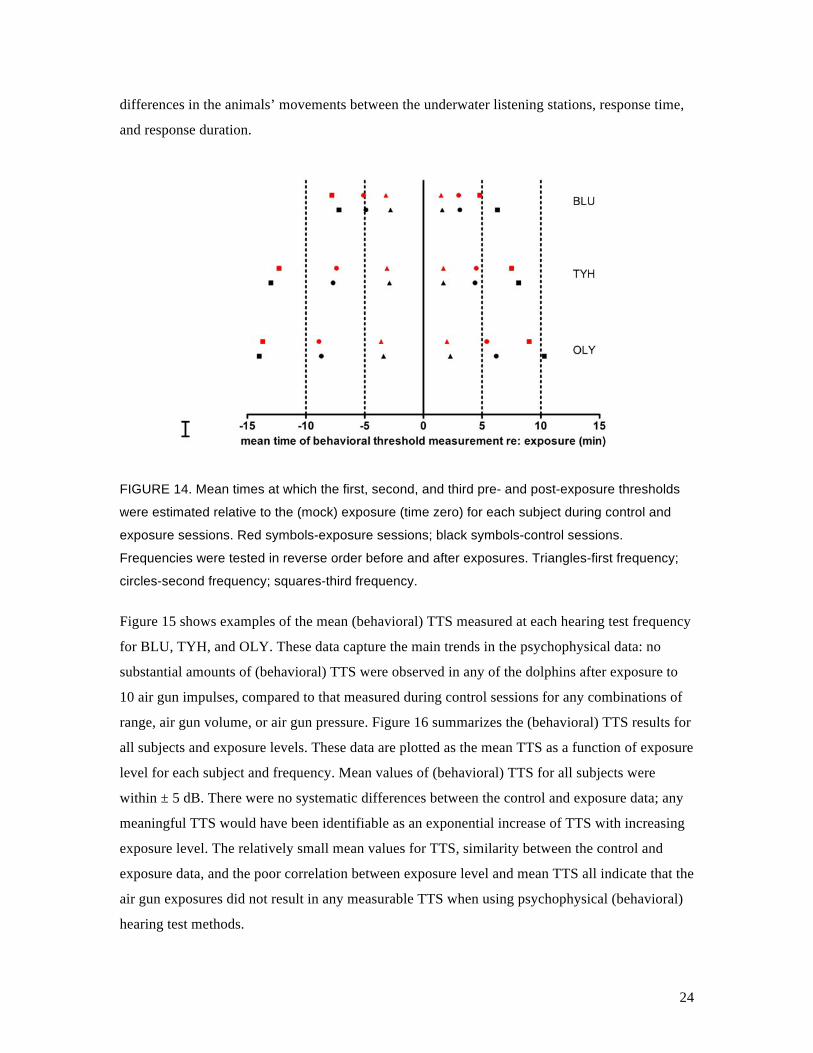
Pre-exposure behavioral thresholds were normally within ± 3 dB of baseline thresholds. Figure 14
depicts the mean time at which the first, second, and third pre- and post-exposure thresholds were
estimated relative to the exposure (time zero) for each subject during control and exposure
sessions. The first post-exposure threshold was typically estimated within 2–4 minutes. In the
case of BLU and TYH, at least two frequencies were normally tested within 5 min after the final
air gun impulse was fired. In most cases, post-exposure thresholds were measured more quickly
than pre-exposure thresholds. The between-subject differences can be attributed to both the two
different computer operators who ran the tests for BLU and for TYH and OLY, and to individual
24
differences in the animals’ movements between the underwater listening stations, response time,
and response duration.
FIGURE 14. Mean times at which the first, second, and third pre- and post-exposure thresholds
were estimated relative to the (mock) exposure (time zero) for each subject during control and
exposure sessions. Red symbols-exposure sessions; black symbols-control sessions.
Frequencies were tested in reverse order before and after exposures. Triangles-first frequency;
circles-second frequency; squares-third frequency.
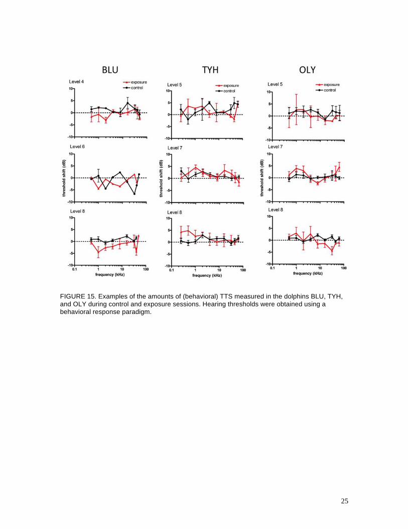
Figure 15 shows examples of the mean (behavioral) TTS measured at each hearing test frequency
for BLU, TYH, and OLY. These data capture the main trends in the psychophysical data: no
substantial amounts of (behavioral) TTS were observed in any of the dolphins after exposure to
10 air gun impulses, compared to that measured during control sessions for any combinations of
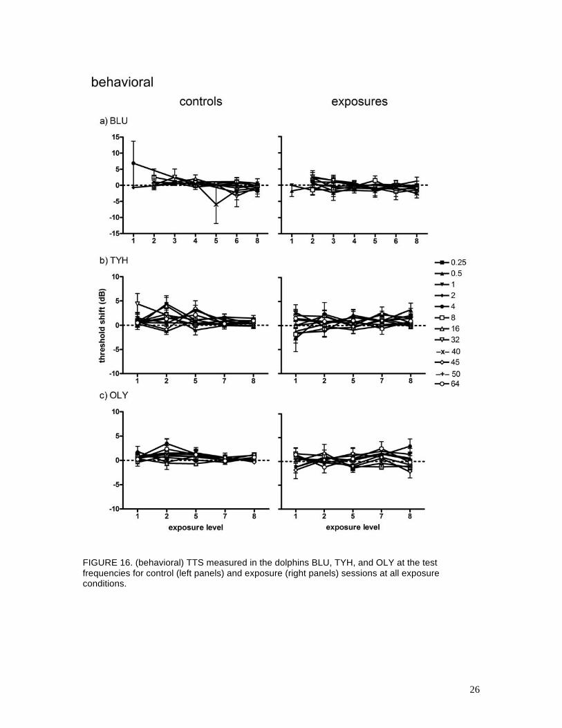
range, air gun volume, or air gun pressure. Figure 16 summarizes the (behavioral) TTS results for
all subjects and exposure levels. These data are plotted as the mean TTS as a function of exposure
level for each subject and frequency. Mean values of (behavioral) TTS for all subjects were
within ± 5 dB. There were no systematic differences between the control and exposure data; any
meaningful TTS would have been identifiable as an exponential increase of TTS with increasing
exposure level. The relatively small mean values for TTS, similarity between the control and
exposure data, and the poor correlation between exposure level and mean TTS all indicate that the
air gun exposures did not result in any measurable TTS when using psychophysical (behavioral)
hearing test methods.
25
FIGURE 15. Examples of the amounts of (behavioral) TTS measured in the dolphins BLU, TYH, and OLY during control and exposure sessions. Hearing thresholds were obtained using a behavioral response paradigm.
26
FIGURE 16. (behavioral) TTS measured in the dolphins BLU, TYH, and OLY at the test frequencies for control (left panels) and exposure (right panels) sessions at all exposure conditions.
27
c. AEP testing
Pre- and post-exposure AEP hearing tests were conducted before and after the behavioral hearing
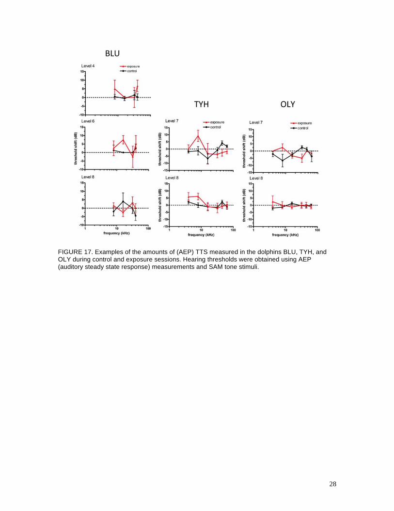
tests at Levels 4–8 for BLU, and at Levels 7 and 8 for TYH and OLY. Figure 17 shows examples
of the mean (AEP) TTS thresholds measured at each hearing test frequency for BLU, TYH, and
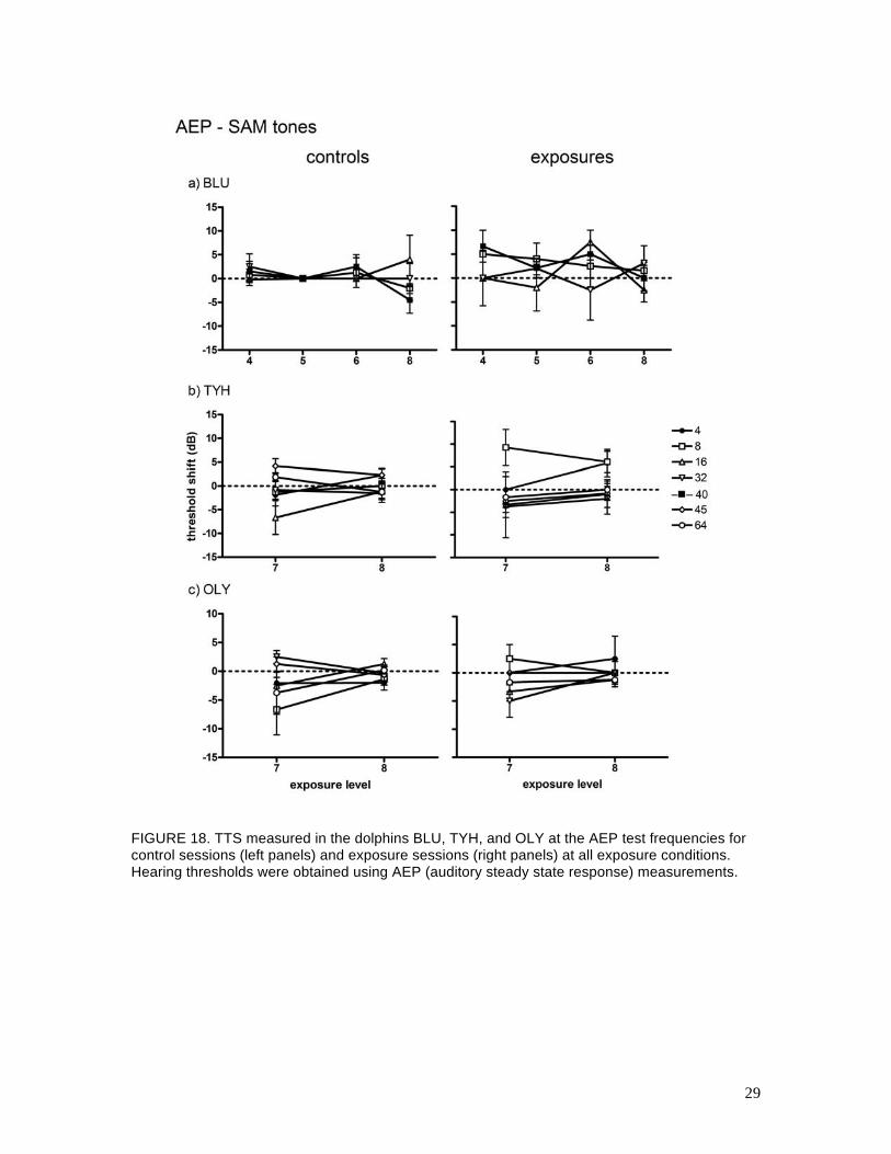
OLY. Figure 18 summarizes the (AEP) TTS results for all subjects and exposure levels. Figures
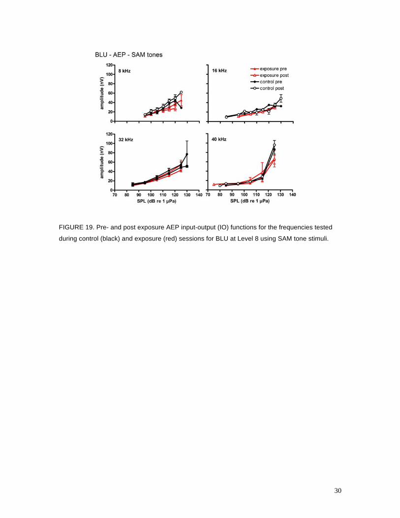
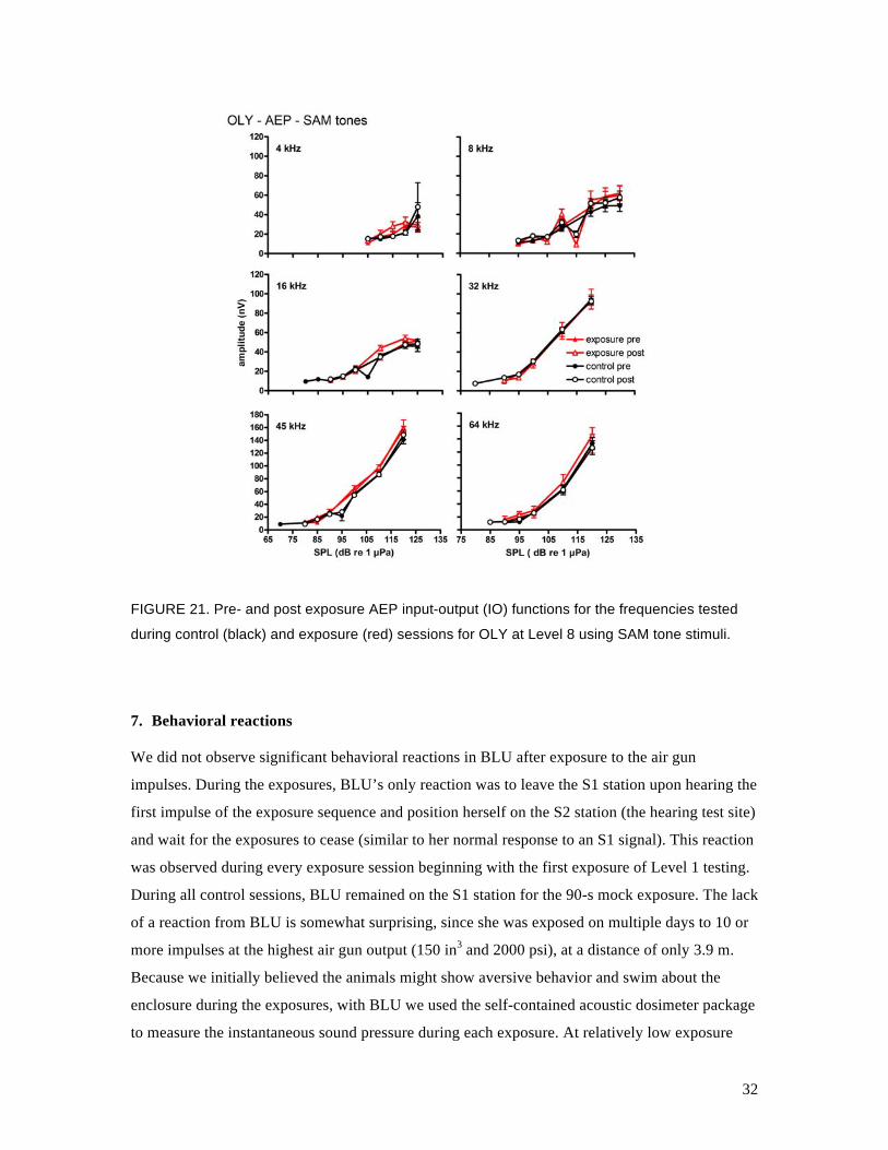
17 and 18 are analogous to Figs. 15 and 16 for the behavioral data. Figures 19, 20, and 21 show
the relationship between the mean ASSR amplitude and the SAM tone SPL (called the input-
output, or IO function) for BLU, TYH, and OLY, respectively, for control and Level 8 exposure
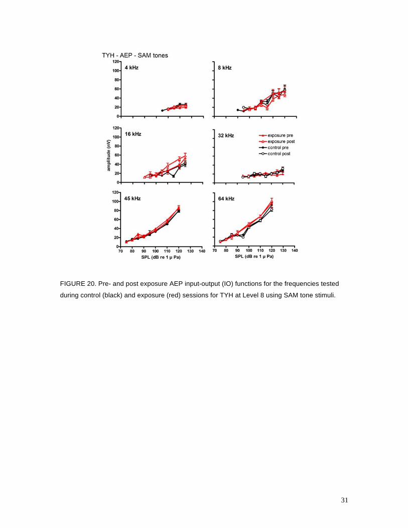
sessions. The AEP data were more variable than the behavioral data and many of the AEP IO
functions were shallow, especially for TYH, which made statistical detection of AEPs near
threshold difficult. Overall, there were no clear differences between the control and exposure
AEP thresholds for BLU or OLY. The IO functions for the pre- and post-exposure sessions were
also very similar for BLU and OLY. For TYH, there were no differences between mean AEP
thresholds except at 8 kHz, where TTSs of 9 and 6 dB were measured after the Level 7 and Level
8 exposures, respectively. Standard deviations about these mean values were high (10 and 7 dB,
respectively) and there was little difference between the pre- and post-exposure IO functions. It is
unusual that the mean TTS actually decreased from Level 7 to Level 8; however, the exposure
SEL increased only 1 dB between these conditions and TYH’s anticipatory behavior may have
affected the resulting TTS (see Sections 7 and 8).
28
FIGURE 17. Examples of the amounts of (AEP) TTS measured in the dolphins BLU, TYH, and OLY during control and exposure sessions. Hearing thresholds were obtained using AEP (auditory steady state response) measurements and SAM tone stimuli.
29
FIGURE 18. TTS measured in the dolphins BLU, TYH, and OLY at the AEP test frequencies for control sessions (left panels) and exposure sessions (right panels) at all exposure conditions. Hearing thresholds were obtained using AEP (auditory steady state response) measurements.
30
FIGURE 19. Pre- and post exposure AEP input-output (IO) functions for the frequencies tested
during control (black) and exposure (red) sessions for BLU at Level 8 using SAM tone stimuli.
31
FIGURE 20. Pre- and post exposure AEP input-output (IO) functions for the frequencies tested
during control (black) and exposure (red) sessions for TYH at Level 8 using SAM tone stimuli.
32
FIGURE 21. Pre- and post exposure AEP input-output (IO) functions for the frequencies tested
during control (black) and exposure (red) sessions for OLY at Level 8 using SAM tone stimuli.
7. Behavioral reactions
We did not observe significant behavioral reactions in BLU after exposure to the air gun
impulses. During the exposures, BLU’s only reaction was to leave the S1 station upon hearing the
first impulse of the exposure sequence and position herself on the S2 station (the hearing test site)
and wait for the exposures to cease (similar to her normal response to an S1 signal). This reaction
was observed during every exposure session beginning with the first exposure of Level 1 testing.
During all control sessions, BLU remained on the S1 station for the 90-s mock exposure. The lack
of a reaction from BLU is somewhat surprising, since she was exposed on multiple days to 10 or
more impulses at the highest air gun output (150 in3 and 2000 psi), at a distance of only 3.9 m.
Because we initially believed the animals might show aversive behavior and swim about the
enclosure during the exposures, with BLU we used the self-contained acoustic dosimeter package
to measure the instantaneous sound pressure during each exposure. At relatively low exposure
33
levels, TYH and OLY both remained on the S1 listening station for the 10-impulse exposure
sequences. After TYH and OLY showed little reaction to the initial exposures, we replaced the
dosimeter with cabled hydrophones attached to the subject via suction cups near the location of
the ears. This allowed a more accurate measurement of the exposure levels using higher sampling
rates.
TYH continued to show little reaction to the exposures from the 10 air gun impulses through
Level 7. For almost all of the 40 exposure sessions at Levels 1, 2, 5, and 7, TYH remained on the
S1 listening station for the 10 impulses, then responded to an underwater buzzer sounded by the
trainer to come to the surface for fish reward before continuing to the S2 station. This was TYH’s
“usual” behavior in previous TTS experiments conducted in an indoor pool. During TYH’s first
Level 8 exposure, with a mean SEL approximately 3 dB higher than his Level 7 exposures, he left
the S1 station after the first impulse and came to the surface. He was at the surface with his ears
and suction-cup hydrophones underwater for the second impulse, was on his way back down to
the S1 station when the third impulse fired, and was back on the S1 station for the remaining
seven impulses. This behavior of leaving S1 and going to the surface after the first impulse
occurred for all remaining exposure sessions. Usually he was at the surface for one or two
impulses before heading back down to station on the S1 biteplate for the rest of the impulse
sequence. On a couple of occasions, he came to the surface twice in the impulse sequence, but
returned to the listening station each time.
On the ninth exposure session at Level 8, TYH began the impulse series as he had in the previous
eight exposures. Then, after returning to the S1 station after coming up to the surface, TYH first
stationed on S1, then backed off the S1 biteplate and turned his head to the (left) side while the
impulse fired, and then stationed back on the biteplate. Just before the next impulse fired, he
backed off again, turned to the side for the next impulse, and then re-stationed on S1. He did this
on/off/on behavior — apparently anticipating the next impulse based on the fixed 10-s inter-
impulse interval — for impulses number 7 through 10 of this series. TYH continued to do this
timing sequence for all remaining exposures at Level 8, and for the follow-on tests at Levels 5, 7
and 8 (see Sect. 8 – Follow-on tests).
OLY’s behavioral reactions to the exposures were more pronounced than BLU and TYH. In most
cases for Levels 1, 2 and 5, OLY came up to the surface after the first impulse, was at the surface
for the second impulse, and then headed back down to S1 and stationed there for the remaining
seven or eight impulses. For OLY’s first exposure at Level 7, he left the S1 station twice during
34
the impulse sequence, but returned each time. For his next three exposure sessions, he reverted to
only leaving the S1 station once after the initial impulse, and then remained on the biteplate. On
his fifth exposure at Level 7, OLY left the S1 station after the first impulse and swam a circle
around the test enclosure before re-stationing for impulses 4–10. For the next several Level 7
exposures, OLY surfaced either once or twice during the exposure sequence, and sometimes
swam a circle before re-stationing on S1. OLY began wearing the suction cup hydrophones on his
11th exposure session at Level 7. Beginning with the 15th Level 7 exposure, OLY left the S1
station after the first impulse and floated at the surface generally facing away from the trainer and
approximately 3.8 m farther away from the S1 station and the air gun for the remaining impulses
before beginning his post-exposure hearing tests. Although he occasionally returned to the S1
station for a couple of impulses before resurfacing, floating near the surface was his typical
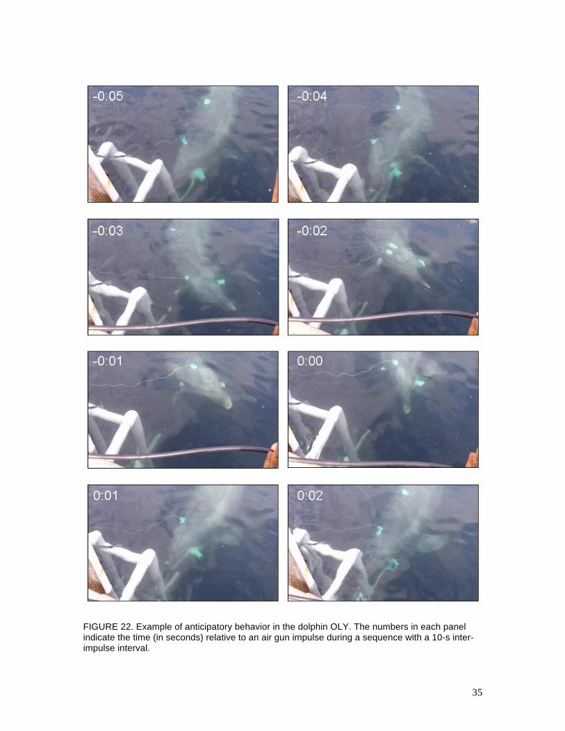
reaction for the remainder of Phase 1 tests and for the follow-on tests. During OLY’s 11th
exposure at Level 8, he exhibited the anticipatory behavior for impulses 7–10 that TYH had
shown: stationing on S1, backing off and turning sideways (left) for the impulse, then re-
stationing on S1 until the next impulse fired (Fig. 22). Unlike TYH who just moved his head off
to the side during the impulses, OLY turned his whole body to the side. OLY did this behavior on
only a couple of occasions for the remainder of Phase 1 testing, but he did it on several occasions
during the follow-on tests (see Sect. 8 – Follow-on tests).
Due to alterations in the trained behavior at the highest level(s) in these two subjects, no attempt
was made to increase the number of impulses beyond 10. As can be seen by the SELs and
standard deviations at Levels 7 and 8 for TYH and OLY, it was clear that their movement around
the S1 station the test enclosure was having some dampening effect on their received levels.
Increasing the number of impulses to increase the cumulative sound exposure in an attempt to
elicit a measureable TTS would be ineffective if the subjects were able to mitigate exposure
levels.
It is important to note that this study was designed to measure TTS, not behavioral reactions, and
substantial effort was made to desensitize two of the three dolphins (BLU and TYH) to the air
gun exposures. Thus, any behavioral observations must be treated with caution and they may not
be representative of wild and/or naïve animals. However, the behavioral data do have some
relative value, in that we have previously seen much more dramatic behavioral reactions in
trained dolphins exposed to other impulsive and steady-state noise conditions (e.g., Finneran et
al., 2002; Schlundt et al., 2000).
35
FIGURE 22. Example of anticipatory behavior in the dolphin OLY. The numbers in each panel indicate the time (in seconds) relative to an air gun impulse during a sequence with a 10-s inter-impulse interval.
36
The anticipatory behavior exhibited by both TYH and OLY is intriguing. Both subjects obviously
learned the timing characteristics of the exposure sequences and eventually adopted the same
posture during the exposures, even turning their heads the same direction. This occurred despite
the two subjects never having been at the test enclosure at the same time during testing; i.e., they
could not have observed the other animal’s behavior during any exposures.
8. Follow-on tests
a. Repeat exposures at lower levels to assess alterations in behavior
At the completion of Phase 1 tests through Level 8, TYH and OLY were re-tested at Levels 7 and
5 with the intent of monitoring their behavior, specifically to see whether they might resume their
previous behavior at those levels and remain on the S1 station during exposure. Both behavioral
and AEP thresholds were measured pre- and post-exposure as in Phase 1 tests. Level 7 was
repeated first. TYH participated in three exposure sessions and OLY participated in two exposure
sessions. Their behavior during the impulsive sound exposures remained the same as during the
Level 8 exposures in the weeks before. Both subjects came to the surface for several impulses,
and if they returned to the S1 station, they left the S1 biteplate just before the impulse fired and
returned during the inter-stimulus interval. The same behaviors were observed when TYH and
OLY each participated in five additional exposures at Level 5. Although TYH stayed on the S1
biteplate for some consecutive impulses, he continued the behavior of surfacing at least once
during the exposures and anticipated many of the remaining impulses. Received exposure levels
during this repeat testing for TYH were very similar to those shown in Table II for Levels 5 and
7. The SELs for OLY at Level 7 were 4 dB lower than in the Phase 1 tests, and at Level 5 they
were 6 dB lower. Because the data collected in these follow-on tests were not consistent with data
in Phase 1 tests before the altered behavior began and the SELs reduced, they were not included
in the TTS results presented above. Control sessions were interspersed between these follow-on
exposures and because the subjects’ behavior was consistent with prior controls, the behavioral
and AEP threshold data from the control sessions were included in the Phase 1 results.
b. Repeat AEP measurements using tone pip stimuli
The IO functions in response to the SAM tones were particularly shallow, especially in the case
of TYH, so additional AEP measurements were conducted at Level 8 using tone pip stimuli
which typically generate a larger brainstem response and could reveal more obvious differences
between pre- and post-exposure IO functions, if any existed. The data for 11 control and 10
37
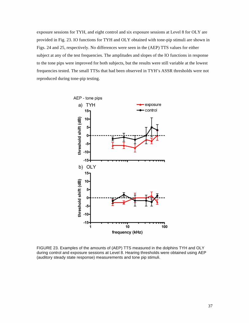
exposure sessions for TYH, and eight control and six exposure sessions at Level 8 for OLY are
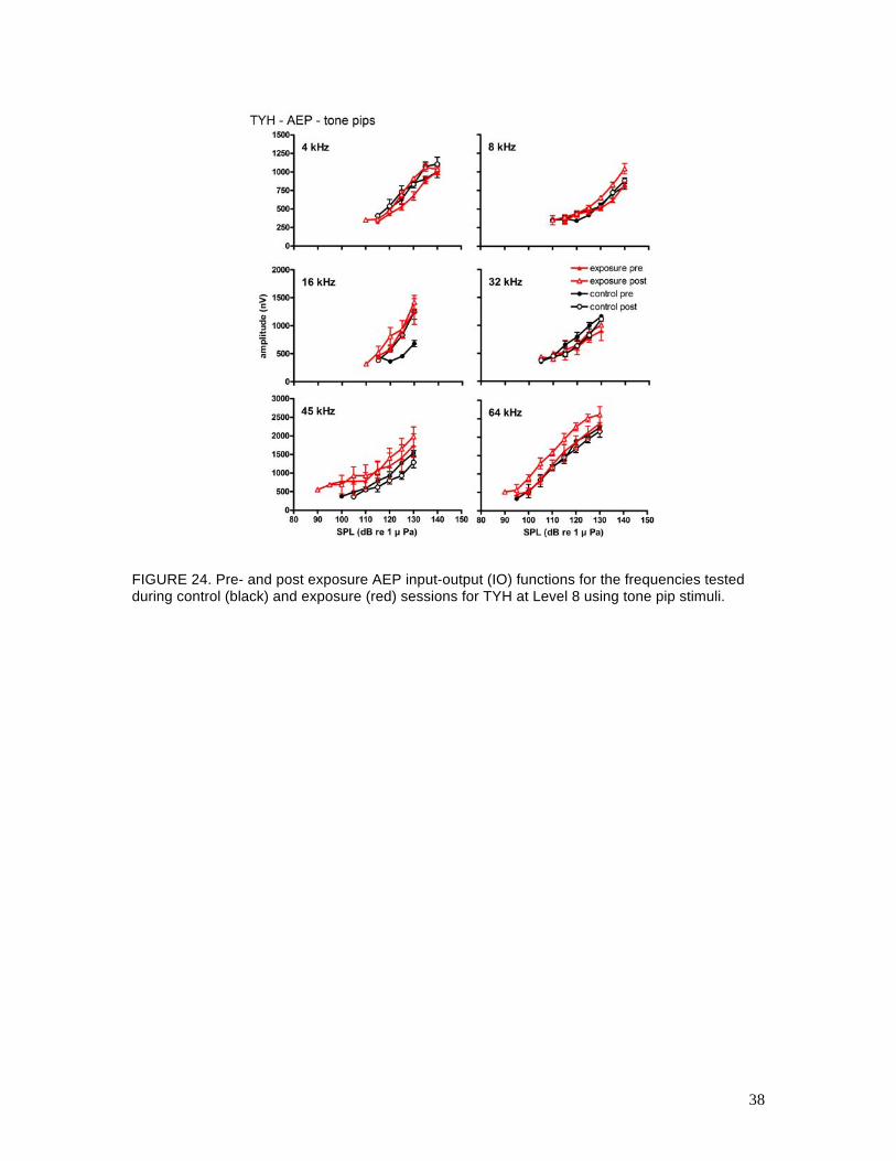
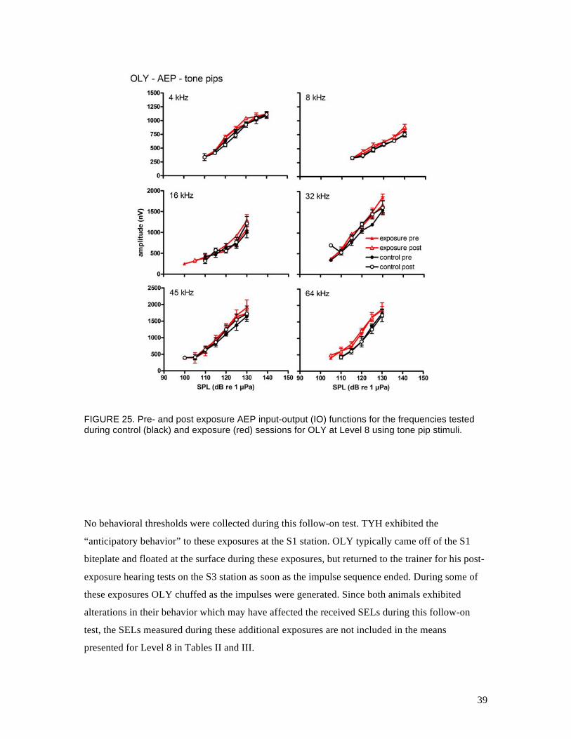
provided in Fig. 23. IO functions for TYH and OLY obtained with tone-pip stimuli are shown in
Figs. 24 and 25, respectively. No differences were seen in the (AEP) TTS values for either
subject at any of the test frequencies. The amplitudes and slopes of the IO functions in response
to the tone pips were improved for both subjects, but the results were still variable at the lowest
frequencies tested. The small TTSs that had been observed in TYH’s ASSR thresholds were not
reproduced during tone-pip testing.
FIGURE 23. Examples of the amounts of (AEP) TTS measured in the dolphins TYH and OLY during control and exposure sessions at Level 8. Hearing thresholds were obtained using AEP (auditory steady state response) measurements and tone pip stimuli.
38
FIGURE 24. Pre- and post exposure AEP input-output (IO) functions for the frequencies tested during control (black) and exposure (red) sessions for TYH at Level 8 using tone pip stimuli.
39
FIGURE 25. Pre- and post exposure AEP input-output (IO) functions for the frequencies tested during control (black) and exposure (red) sessions for OLY at Level 8 using tone pip stimuli.
No behavioral thresholds were collected during this follow-on test. TYH exhibited the
“anticipatory behavior” to these exposures at the S1 station. OLY typically came off of the S1
biteplate and floated at the surface during these exposures, but returned to the trainer for his post-
exposure hearing tests on the S3 station as soon as the impulse sequence ended. During some of
these exposures OLY chuffed as the impulses were generated. Since both animals exhibited
alterations in their behavior which may have affected the received SELs during this follow-on
test, the SELs measured during these additional exposures are not included in the means
presented for Level 8 in Tables II and III.
40
c. Steady-state ASSR measurements during exposures
It seems likely that the “anticipatory” behavior displayed by both TYH and OLY was related in
some manner to mitigating the perceived level and/or auditory effects of the impulsive noise
exposure. To investigate whether hearing sensitivity in TYH and OLY actually changed while
they performed this behavior, exposures were conducted while hearing sensitivity was
simultaneously monitored via the ASSR in response to a continuous sinusoidal amplitude
modulated (SAM) tone. The SAM tone carrier frequencies (i.e., the hearing test frequency) were
the ones that produced the largest ASSRs: 40 kHz for OLY and 60 kHz for TYH. The SAM tone
modulation rates were 1 kHz. SAM tones were continuously delivered to each subject via a
“jawphone” transducer — a piezoelectric transducer embedded in a suction cup and attached to
the lower jaw. The jawphone was used to maintain a constant stimulus level even if the subjects
moved. The instantaneous EEG was obtained from the potential difference between surface
electrodes placed on the head and back and saved to disk over 120-s epochs before, during, and
after exposure to the air gun impulses. The synchronization pulse used to trigger the air gun was
also saved to disk. During offline analysis, the instantaneous EEG was first divided into 30-ms
epochs. Time-averaging was then performed on each collection of 128 sequential epochs. Each
average was then Fourier transformed to obtain the frequency spectrum. The ASSR amplitude
was defined as the spectral amplitude at the SAM tone modulation rate (1 kHz). Successive
averaging periods were overlapped by 50%. To avoid electrical or acoustical artifacts from the air
gun triggering or impulse, epochs existing within ±200 ms of the air gun impulses were excluded
from averaging. Measurements were made seven times with OLY and TYH. Each measurement
consisted of a pre-exposure, exposure, and post-exposure session. The air gun firing was
simulated, and the air gun trigger pulse recorded to disk but not used to fire the air gun, during the
pre- and post-exposure sessions.
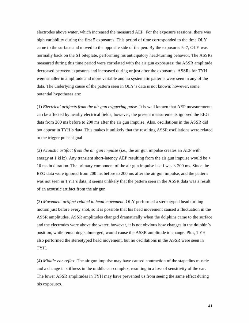
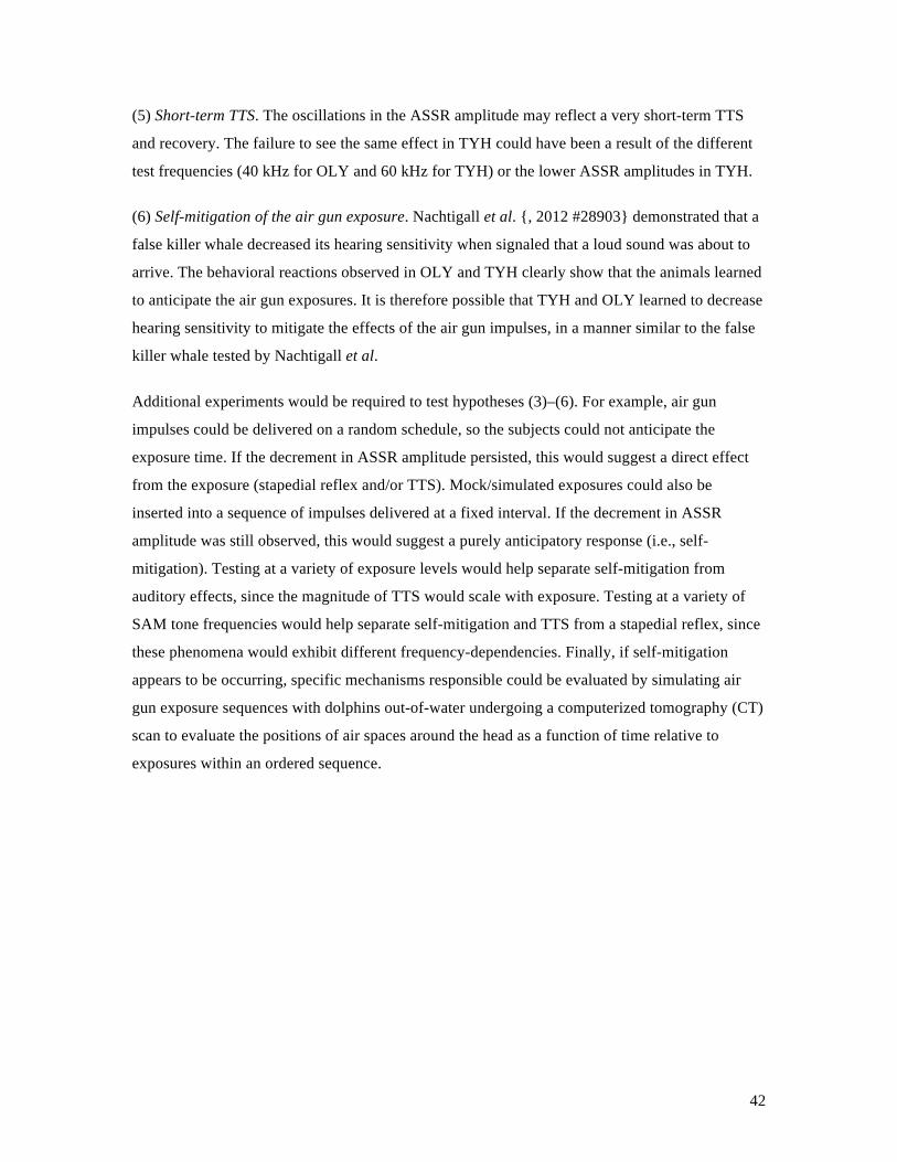
Figures 26 and 27 show the ASSR amplitudes as functions of time for the pre-exposure,
exposure, and post-exposure sessions for OLY and TYH, respectively. Within each plot, ASSR
measurements from different days are overlaid. If the subject remained stationary, one would
expect the ASSR amplitude to remain relatively constant over time and there should be no
correlation between the air gun exposures (or simulated air gun exposures) and the ASSR
amplitudes. For OLY, the ASSR amplitudes measured during the pre-exposure and post-exposure
sessions were relatively stable over time (as expected) and were not correlated with the timing of
the simulated air gun exposures. Salient peaks in the post-exposure data (e.g., OLY’s post-
exposure data at 30-s) correspond to the subject coming to the surface and putting one or more
41
electrodes above water, which increased the measured AEP. For the exposure sessions, there was
high variability during the first 5 exposures. This period of time corresponded to the time OLY
came to the surface and moved to the opposite side of the pen. By the exposures 5–7, OLY was
normally back on the S1 biteplate, performing his anticipatory head-turning behavior. The ASSRs
measured during this time period were correlated with the air gun exposures: the ASSR amplitude
decreased between exposures and increased during or just after the exposures. ASSRs for TYH
were smaller in amplitude and more variable and no systematic patterns were seen in any of the
data. The underlying cause of the pattern seen in OLY’s data is not known; however, some
potential hypotheses are:
(1) Electrical artifacts from the air gun triggering pulse. It is well known that AEP measurements
can be affected by nearby electrical fields; however, the present measurements ignored the EEG
data from 200 ms before to 200 ms after the air gun impulse. Also, oscillations in the ASSR did
not appear in TYH’s data. This makes it unlikely that the resulting ASSR oscillations were related
to the trigger pulse signal.
(2) Acoustic artifact from the air gun impulse (i.e., the air gun impulse creates an AEP with
energy at 1 kHz). Any transient short-latency AEP resulting from the air gun impulse would be <
10 ms in duration. The primary component of the air gun impulse itself was < 200 ms. Since the
EEG data were ignored from 200 ms before to 200 ms after the air gun impulse, and the pattern
was not seen in TYH’s data, it seems unlikely that the pattern seen in the ASSR data was a result
of an acoustic artifact from the air gun.
(3) Movement artifact related to head movement. OLY performed a stereotyped head turning
motion just before every shot, so it is possible that his head movement caused a fluctuation in the
ASSR amplitudes. ASSR amplitudes changed dramatically when the dolphins came to the surface
and the electrodes were above the water; however, it is not obvious how changes in the dolphin’s
position, while remaining submerged, would cause the ASSR amplitude to change. Plus, TYH
also performed the stereotyped head movement, but no oscillations in the ASSR were seen in
TYH.
(4) Middle-ear reflex. The air gun impulse may have caused contraction of the stapedius muscle
and a change in stiffness in the middle ear complex, resulting in a loss of sensitivity of the ear.
The lower ASSR amplitudes in TYH may have prevented us from seeing the same effect during
his exposures.
42
(5) Short-term TTS. The oscillations in the ASSR amplitude may reflect a very short-term TTS
and recovery. The failure to see the same effect in TYH could have been a result of the different
test frequencies (40 kHz for OLY and 60 kHz for TYH) or the lower ASSR amplitudes in TYH.
(6) Self-mitigation of the air gun exposure. Nachtigall et al. {, 2012 #28903} demonstrated that a
false killer whale decreased its hearing sensitivity when signaled that a loud sound was about to
arrive. The behavioral reactions observed in OLY and TYH clearly show that the animals learned
to anticipate the air gun exposures. It is therefore possible that TYH and OLY learned to decrease
hearing sensitivity to mitigate the effects of the air gun impulses, in a manner similar to the false
killer whale tested by Nachtigall et al.
Additional experiments would be required to test hypotheses (3)–(6). For example, air gun
impulses could be delivered on a random schedule, so the subjects could not anticipate the
exposure time. If the decrement in ASSR amplitude persisted, this would suggest a direct effect
from the exposure (stapedial reflex and/or TTS). Mock/simulated exposures could also be
inserted into a sequence of impulses delivered at a fixed interval. If the decrement in ASSR
amplitude was still observed, this would suggest a purely anticipatory response (i.e., self-
mitigation). Testing at a variety of exposure levels would help separate self-mitigation from
auditory effects, since the magnitude of TTS would scale with exposure. Testing at a variety of
SAM tone frequencies would help separate self-mitigation and TTS from a stapedial reflex, since
these phenomena would exhibit different frequency-dependencies. Finally, if self-mitigation
appears to be occurring, specific mechanisms responsible could be evaluated by simulating air
gun exposure sequences with dolphins out-of-water undergoing a computerized tomography (CT)
scan to evaluate the positions of air spaces around the head as a function of time relative to
exposures within an ordered sequence.
43
FIGURE 26. ASSR amplitudes as a function of time (a) before, (b) during, and (c) after exposure to air gun impulses for OLY. The vertical dashed lines indicate the times of the air gun exposures in (b) and the simulated exposures in (a), (c). Each trace represents an ASSR measurement from a different day.
44
FIGURE 27. ASSR amplitudes as a function of time (a) before, (b) during, and (c) after exposure to air gun impulses for TYH. The vertical dashed lines indicate the times of the air gun exposures in (b) and the simulated exposures in (a), (c). Each trace represents an ASSR measurement from a different day.
45
VII. Significance
At the cessation of the study, the dolphins BLU, TYH and OLY showed no clear (behavioral)
TTS after exposure to 10 impulses from a single, 150 in3 air gun operating at 2000 psi and located
at a range of 3.9 m (total cumulative SEL = ~189–195 dB re 1 µPa2s). These data contrast with
earlier studies where a beluga experienced TTS after exposure to a single impulse from a
watergun (SEL = 186 dB re 1 µPa2s; Finneran et al., 2002) and a harbor porpoise exhibited TTS
after exposure to a single air gun pulse (SEL = 164 dB re 1 µPa2s; Lucke et al., 2009). The
occurrence of TTS in the porpoise exposed to lower level air gun exposures is consistent with the
increased susceptibility of porpoises to noise (compared to dolphins) observed in TTS studies
utilizing broadband noise (Kastelein et al., 2011; Popov et al., 2011). The differences between the
watergun effects on the beluga and the air gun effects on the dolphins BLU, TYH, and OLY are a
little more surprising, since they were exposed to 10 impulses and the SEL from a single impulse
was close to that of the watergun.
Potential explanations why (behavioral) TTS was not observed in BLU, TYH, or OLY at any of
the exposure conditions include the following:
(1) Dolphins may be relatively insensitive to impulsive noise exposures. This idea is bolstered by
the lack of TTS in the dolphin exposed a watergun impulse with SEL = 188 dB re 1 µPa2s, but
contradicted by anatomical data, auditory capability data, and tonal TTS data for dolphins and
belugas which show very similar results between dolphins and belugas.
(2) There was little to no accumulation of effect across the multiple exposures. The single
impulse SEL values for the airgun exposures were slightly lower than those from the watergun. It
is possible that the inter-impulse interval was long enough to prevent accumulation of effects for
the 10 impulses.
(3) The air gun exposures were inherently less hazardous than watergun exposures with the same
SEL. Although predictions based on the single impulse SEL from the watergun data suggested
that TTS should have occurred, the exposure scenarios may have actually been well below those
capable of inducing TTS; i.e., unweighted SEL may not the best metric to predict auditory effects
from impulsive sources like waterguns and air guns.
The two primary differences between the air gun and watergun exposures were the peak pressure
and the frequency content. The p-p SPL of the watergun impulse that produced TTS was 228 dB
re 1 µPa, 16–29 dB higher than the maximum p-p SPLs the dolphins were exposed to in the
46
present study. If p-p SPL was used as the main predictor of TTS, we should not be surprised that
the watergun produced TTS and the air gun exposure did not. The extent to which the p-p SPL of
the air gun impulse was affected by the test environment is unknown; i.e., it is not known if the
same relationship between p-p SPL for an air gun and watergun impulse with the same SEL
would exist in other environments.
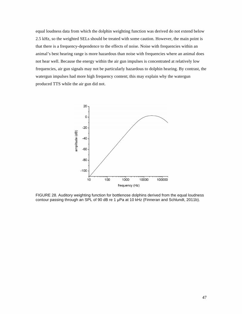
The relatively low frequency content in the air gun impulses may also have little effect on
dolphins, whose best hearing sensitivity occurs at much higher frequencies. The frequency-
dependent effects of noise are typically handled by applying a “weighting function” that adjust
the frequency spectrum of the noise to emphasize noise frequencies where the listener is sensitive
to noise and to de-emphasize frequencies where sensitivity to noise is low. For humans, the most
commonly used weighting functions are the “A-weighting” and “C-weighting” functions
[American National Standard Institute (ANSI), 2006]. These functions were derived from equal
loudness contours for human listeners—curves representing the combinations of SPL and
frequency that are perceived as equally loud to human listeners.
Historically, equal loudness contours did not exist for animals, therefore, auditory weighting
functions for marine mammals were based on auditory sensitivity curves (e.g., Nedwell et al.,
2007) or known or suspected audible bandwidths (e.g., Southall et al., 2007). Recently, subjective
loudness level measurements have been performed with the bottlenose dolphin TYH, and the
resulting data have been used to derive equal loudness contours and auditory weighting functions
(Fig. 28; Finneran and Schlundt, 2011b) that agree closely with dolphin TTS onset data obtained
from tonal exposures at 3 to 56 kHz (Finneran and Schlundt, 2011a). We can use this weighting
function to estimate the “effective” exposure level for the air gun impulses compared to other
noise sources.
Figures 29 and 30 show representative examples of the pressure-time waveforms and frequency
spectra for the watergun exposure that caused TTS in a beluga (Finneran et al., 2002) and the
maximum single air gun impulse received by BLU in the present study. The mean SELs for these
two exposure conditions were identical: 186 dB re 1 µPa2s. However, the watergun exposure had
a larger peak-peak pressure, faster rise-time, shorter duration, and more high-frequency content
compared to the air gun exposure. When the dolphin weighting function is applied, the weighted
SELs fall to 173 dB re 1 µPa2s for the watergun impulse and 144 dB re 1 µPa2s for the air gun.
So, when taking into account the frequency-dependent sensitivity of the dolphin auditory system,
the air gun impulses appear much less hazardous than the watergun impulses. Of course, the
47
equal loudness data from which the dolphin weighting function was derived do not extend below
2.5 kHz, so the weighted SELs should be treated with some caution. However, the main point is
that there is a frequency-dependence to the effects of noise. Noise with frequencies within an
animal’s best hearing range is more hazardous than noise with frequencies where an animal does
not hear well. Because the energy within the air gun impulses is concentrated at relatively low
frequencies, air gun signals may not be particularly hazardous to dolphin hearing. By contrast, the
watergun impulses had more high frequency content; this may explain why the watergun
produced TTS while the air gun did not.
FIGURE 28. Auditory weighting function for bottlenose dolphins derived from the equal loudness contour passing through an SPL of 90 dB re 1 µPa at 10 kHz (Finneran and Schlundt, 2011b).

48
FIGURE 29. Representative pressure-time waveforms for the watergun impulsive noise exposure that caused TTS in a beluga (Finneran et al., 2002) and the maximum air gun exposure for BLU from the present study.
FIGURE 30. Representative spectra for the watergun impulsive noise exposure that caused TTS in a beluga (Finneran et al., 2002) and the maximum air gun exposure for BLU from the present study (150 in3, 2000 psi, 3.9 m). The sound exposure spectral density levels in the lower panel have been “weighted” by applying the dolphin weighting function based on the 90 dB re 1 µPa equal loudness contour (Finneran and Schlundt, 2011b).
49
Overall, the AEP measurements were inconclusive. No measurable TTS was seen in BLU or
OLY. A small mean TTS was produced in TYH after the Level 7 exposures, but this could not be
replicated at higher exposure levels or using tone-pip stimuli. The interpretation of these results is
clouded by TYH’s behavioral reactions — it is possible that the failure to reproduce the TTS seen
at 8 kHz was due to TYH’s self-mitigation of the noise exposure.
VIII. Conclusions
This project demonstrated that an air gun could be safely operated within San Diego Bay using
visual observers and safety ranges to prevent exposure of protected species to potentially harmful
levels. TTS measurements can be safely conducted with dolphins exposed to various
combinations of air gun volume and pressure and at various distances, and, if the exposure levels
are gradually increased, dolphins may show little reaction to the air gun impulses, even at ranges
as close as 3.9 m and with the air gun operating at 150 in3 and 2000 psi. At the highest exposure
levels, two of the dolphins anticipated the exposures and adopted postures which suggested that
they were attempting to mitigate the effects.
Exposures of up to 10 impulses from a 150 in3 air gun operating at 2000 psi (cumulative SEL of
189–195 dB re 1 µPa2s) did not produce clear, reliable TTS in any of the three dolphins; this may
be a result of the relatively low frequency content of the air gun impulses compared to the
dolphin’s range of best hearing or the lower p-p SPL compared to earlier impulsive sources. The
data from this study are consistent with the weighted SEL and p-p SPL criteria from Southall et
al. (2007).
IX. References
American National Standard Institute (ANSI) (2006). “ANSI S1.42-2001 (R 2006) American National Standard Design Response of Weighting Networks for Acoustical Measurements,” (Acoustical Society of America).
Finneran, J. J., Carder, D. A., Schlundt, C. E., and Dear, R. L. (2010a). “Growth and recovery of temporary threshold shift (TTS) at 3 kHz in bottlenose dolphins (Tursiops truncatus),” Journal of the Acoustical Society of America 127, 3256-3266.
Finneran, J. J., Carder, D. A., Schlundt, C. E., and Dear, R. L. (2010b). “Temporary threshold shift in a bottlenose dolphin (Tursiops truncatus) exposed to intermittent tones,” Journal of the Acoustical Society of America 127, 3267-3272.
Finneran, J. J., Carder, D. A., Schlundt, C. E., and Ridgway, S. H. (2005). “Temporary threshold shift (TTS) in bottlenose dolphins (Tursiops truncatus) exposed to mid-frequency tones,” Journal of the Acoustical Society of America 118, 2696-2705.
50
Finneran, J. J., Dear, R., Carder, D. A., and Ridgway, S. H. (2003). “Auditory and behavioral responses of California sea lions (Zalophus californianus) to single underwater impulses from an arc-gap transducer,” Journal of the Acoustical Society of America 114, 1667-1677.
Finneran, J. J. and Schlundt, C. E. (2010). “Frequency-dependent and longitudinal changes in noise-induced hearing loss in a bottlenose dolphin (Tursiops truncatus),” Journal of the Acoustical Society of America 128, 567-570.
Finneran, J. J. and Schlundt, C. E. (2011a). “Auditory weighting functions and acoustic damage risk criteria for marine mammals,” in Fourth Intergovernmental Conference on the Effects of Sound in the Ocean on Marine Mammals (Amsterdam, The Netherlands).
Finneran, J. J. and Schlundt, C. E. (2011b). “Subjective loudness level measurements and equal loudness contours in a bottlenose dolphin (Tursiops truncatus),” Journal of the Acoustical Society of America 130, 3124-3136.
Finneran, J. J., Schlundt, C. E., Branstetter, B., and Dear, R. L. (2007). “Assessing temporary threshold shift in a bottlenose dolphin (Tursiops truncatus) using multiple simultaneous auditory evoked potentials,” Journal of the Acoustical Society of America 122, 1249–1264.
Finneran, J. J., Schlundt, C. E., Carder, D. A., Clark, J. A., Young, J. A., Gaspin, J. B., and Ridgway, S. H. (2000). “Auditory and behavioral responses of bottlenose dolphins (Tursiops truncatus) and a beluga whale (Delphinapterus leucas) to impulsive sounds resembling distant signatures of underwater explosions,” Journal of the Acoustical Society of America 108, 417-431.
Finneran, J. J., Schlundt, C. E., Dear, R., Carder, D. A., and Ridgway, S. H. (2002). “Temporary shift in masked hearing thresholds (MTTS) in odontocetes after exposure to single underwater impulses from a seismic watergun,” Journal of the Acoustical Society of America 111, 2929-2940.
Houser, D. S. and Finneran, J. J. (2006). “Variation in the hearing sensitivity of a dolphin population obtained through the use of evoked potential audiometry,” Journal of the Acoustical Society of America 120, 4090-4099.
Kastak, D., Schusterman, R. J., Southall, B. L., and Reichmuth, C. J. (1999). “Underwater temporary threshold shift induced by octave-band noise in three species of pinniped,” Journal of the Acoustical Society of America 106, 1142-1148.
Kastak, D., Southall, B. L., Schusterman, R. J., and Kastak, C. R. (2005). “Underwater temporary threshold shift in pinnipeds: effects of noise level and duration,” Journal of the Acoustical Society of America 118, 3154-3163.
Kastelein, R., Gransier, R., Mierlo, R. v., Hoek, L., and Jong, C. d. (2011). “Temporary hearing threshold shifts and recovery in a harbor porpoise (Phocoena phocoena) and harbor seals (Phoca vitulina) exposed to white noise in a 1/1�octave band around 4 kHz,” Journal of the Acoustical Society of America 129, 2432 (A).
Lucke, K., Siebert, U., Lepper, P. A., and Blanchet, M.-A. (2009). “Temporary shift in masked hearing thresholds in a harbor porpoise (Phocoena phocoena) after exposure to seismic airair gun stimuli,” Journal of the Acoustical Society of America 125, 4060–4070.
Mooney, T. A., Nachtigall, P. E., Breese, M., Vlachos, S., and Au, W. W. L. (2009). “Predicting temporary threshold shifts in a bottlenose dolphin (Tursiops truncatus): The effects of noise level and duration,” The Journal of the Acoustical Society of America 125, 1816-1826.
51
Nachtigall, P. E., Pawloski, J., and Au, W. W. L. (2003). “Temporary threshold shifts and recovery following noise exposure in the Atlantic bottlenosed dolphin (Tursiops truncatus),” Journal of the Acoustical Society of America 113, 3425-3429.
Nachtigall, P. E., Supin, A. Y., Pawloski, J., and Au, W. W. L. (2004). “Temporary threshold shifts after noise exposure in the bottlenose dolphin (Tursiops truncatus) measured using evoked auditory potentials,” Marine Mammal Science 20, 673-687.
Nedwell, J. R., Turnpenny, A. W. H., Lovell, J., Parvin, S. J., Workman, R., Spinks, J. A. L., and Howell, D. (2007). “A validation of the dBht as a measure of the behavioural and auditory effects of underwater noise,” 534R1231 (Subacoustech Acoustic Research Consultancy).
Popov, V. V., Supin, A. Y., Wang, D., Wang, K., Dong, L., and Wang, S. (2011). “Noise-induced temporary threshold shift and recovery in Yangtze finless porpoises Neophocaena phocaenoides asiaeorientalis,” Journal of the Acoustical Society of America 130, 574-584.
Ridgway, S. H., Carder, D. A., Smith, R. R., Kamolnick, T., Schlundt, C. E., and Elsberry, W. R. (1997). “Behavioral responses and temporary shift in masked hearing thresholds of bottlenose dolphins, Tursiops truncatus, to 1-second tones of 141-201 dB re 1 µPa,” Technical Report 1751 (Naval Command, Control, and Ocean Surveillance Center, RDT&E Division, San Diego, CA).
Schlundt, C. E., Finneran, J. J., Carder, D. A., and Ridgway, S. H. (2000). “Temporary shift in masked hearing thresholds of bottlenose dolphins, Tursiops truncatus, and white whales, Delphinapterus leucas, after exposure to intense tones,” Journal of the Acoustical Society of America 107, 3496-3508.
Southall, B. L., Bowles, A. E., Ellison, W. T., Finneran, J. J., Gentry, R. L., Greene, C. R., Jr., Kastak, D., Ketten, D. R., Miller, J. H., Nachtigall, P. E., Richardson, W. J., Thomas, J. A., and Tyack, P. L. (2007). “Marine mammal noise exposure criteria: initial scientific recommendations,” Aquatic Mammals 33, 411-521.


![Hunterston Jetty · TTS/PTS threshold [dB SEL-24] Impulsive threshold [dB SEL-24] Impulsive threshold [dB z-p] TTS 185 185 197 PTS 213 213 206 1.2.4 APPLICATION OF HEARING THRESHOLDS](https://img.pdfslide.net/doc/110x75/5d1376cc88c993b4258bccb1/hunterston-jetty-ttspts-threshold-db-sel-24-impulsive-threshold-db-sel-24.jpg)