Embed Size (px)
Citation preview
SPECIAL FEATURE
Tensor-Based Shot Boundary Detection in VideoStreams
Bogusław Cyganek1• Michał Wozniak2
Received: 21 April 2017 / Accepted: 28 June 2017 / Published online: 8 August 2017
� The Author(s) 2017. This article is an open access publication
Abstract This paper presents a method for content change detection in multidi-
mensional video signals. Video frames are represented as tensors of order consistent
with signal dimensions. The method operates on unprocessed signals and no special
feature extraction is assumed. The dynamic tensor analysis method is used to build a
tensor model from the stream. Each new datum in the stream is then compared to
the model with the proposed concept drift detector. If it fits, then a model is updated.
Otherwise, a model is rebuilt, starting from that datum, and the signal shot is
recorded. The proposed fast tensor decomposition algorithm allows efficient oper-
ation compared to the standard tensor decomposition method. Experimental results
show many useful properties of the method, as well as its potential further exten-
sions and applications.
Keywords Video shot detection � Anomaly detection � Tensor decomposition �Tensor frames � Dynamic tensor analysis
Introduction
Enormously increasing amounts of visual information raise the needs for the
development of automatic data analysis methods. Among these, special attention is
paid to the video summarization methods. Their goal is to give a user a short and
useful visual abstract of the entire video sequence. This can be further used to
& Bogusław Cyganek
Michał Wozniak
1 AGH University of Science and Technology, Al. Mickiewicza 30, 30-059 Krakow, Poland
2 Wrocław University of Science and Technology, Wybrze _ze Wyspianskiego 27, 50-370 Krakow,
Poland
123
New Gener. Comput. (2017) 35:311–340
DOI 10.1007/s00354-017-0024-0
improve efficacy of video cataloging, indexing, archiving, information search, data
compression, to name a few [47]. These methods, in turn, rely on efficient
algorithms of boundary detection in the visual streams. Basically, the summariza-
tion methods are divided into static and dynamic ones [33, 35]. In the former, a set
of consecutive frames with sufficiently coherent contents is represented by a single
representative frame, called a key frame. On the other hand, a dynamic
summarization, also called a video skim, relies on selecting the most relevant
small fractions of the video sequences [19]. This allows for better representation of
the concise portions of the video, thanks to inclusion of visual and audio tracks. A
key step in these methods is to track a video stream and recognize regions of
sufficiently abrupt change in the visual content. However, such generally stated task
is subjective and depends on specific video content which manifests with different
segmentations done in human-made experiments. For the purpose of automatic
video summarization, a significant research is conducted toward the development of
methods for computation of sufficiently discriminative features [20, 45]. In this
spirit, majority of the methods first employ extraction of specific features, which are
then used for video clusterization and classification.
Our proposed approach to video analysis significantly differs from the feature-
based methods. Most of all we treat the frames holistically as 2D or 3D tensors—
therefore, we call them tensor frames. This way, considering time dimension, the
whole video can be represented as a 4D tensor. Such a framework allows easy
extensions to higher dimensions, if necessary. Further on, we do not extract any
features from the frames which is a common practice in majority of the video
summarization methods proposed in the literature. In addition, in many of the
available works on video segmentation, temporal analysis is not fully exploited.
However, this is a very important factor, since the consecutive frames show high
correlation throughout a scene. On the other hand, our framework allows for a
uniform approach to video structure analysis, both in spatial and temporal
dimensions. Our method relies on the tensor stream processing concept proposed
by Sun et al. [44]. However, in our approach, this method was improved to allow for
efficient processing of the video streams, as will also be discussed. To the best of
our knowledge, the tensor stream tensor analysis method has not been used in the
problem of video summarization. Our contribution is as follows:
• the original tensor framework for video shot detection based on the tensor model
and its continuous build-and-update mechanism;
• novel concept of drift detectors in tensor video streams based on statistical
analysis of the differences of the tensor-frame projections onto the model;
• fast tensor subspace computation with the modified fixed-point eigenvalue
method, endowed with a mechanism of dominant rank determination and re-
initialization from previous eigenvectors.
As mentioned, the proposed method can operate with any dimensional signals,
such as monochrome and color videos, as presented in the experimental section of
this paper. No feature extraction is necessary and the signal is treated ‘‘as is’’.
Therefore, the method can work with frames of any dimension and content, such as
312 New Gener. Comput. (2017) 35:311–340
123
hyperspectral or compressed signals, etc. However, due to the so-called ‘‘curse of
dimensionality’’ when going into higher dimensions, we face the problem of high
memory and computational requirements [4, 55]. In addition, if statistical properties
of the processed signal are known, then feature-based methods can perform better
taking advantage of the expert knowledge. Nonetheless, the proposed framework
can also accept features and signal as its input, as will be discussed.
The rest of this paper is organized as follows. Section 2 outlines the basic
concepts related to video signal representation and analysis, as well as presents
related works in the area of the video segmentation, tensor processing, and data
streams. A short overview on tensors and their decomposition is presented in Sect.
3. The main concepts of the proposed method are presented in Sect. 4. Specifically,
system architecture and basic concepts of tensor stream analysis are presented in
Sect. 4.1, and a modified best rank-(R1, R2, …, RP) tensor decomposition for stream
tensors is discussed in Sect. 4.2. Efficient computation of the dominating tensor
subspace is outlined in Sect. 4.3. Computation of the proposed drift detection in
video tensor streams is presented in Sect. 4.4. Finally, the video tensor stream model
build-and-update scheme is presented in Sect. 4.5. Experimental results are
presented in Sect. 5, while conclusions are presented in Sect. 6.
Overview of Video Signal Representation and Analysis
This section contains a brief introduction to the video representation and signal
analysis methods for the purpose of scene shot detection and video summarization.
Video Structure and Analysis
A video is a multidimensional digital signal organized as a stream of still images,
called frames, as depicted in Fig. 1. These may be monochrome or color images.
Visual signals are accompanied by the audio signal, which is not considered in this
work, though. As will be further discussed, frames as well as videos can be
interpreted as tensors. In this framework, a monochrome frame is represented as a
2D tensor, a color frame as a 3D tensor, and so on. Thus, these are called tensor
frames. Content of frames changes in time-giving impression of smooth motion to
the observer. On the other hand, consecutive frames that contain similar content are
grouped together and form the so-called shots. Finally, a set of consecutive shots
with semantically similar content is called a scene. These are visualized in Fig. 1.
There can be different types of content change in video signals. These can be
grouped as follows:
• Hard cuts—an abrupt change of a content;
• Soft cuts—a gradual change of a content.
The latter can further divided into the following categories:
• Fade-in/out—a new scene gradually appears/disappears from the current image;
• Dissolve—a current shot fades out, whereas the incoming one fades in.
New Gener. Comput. (2017) 35:311–340 313
123
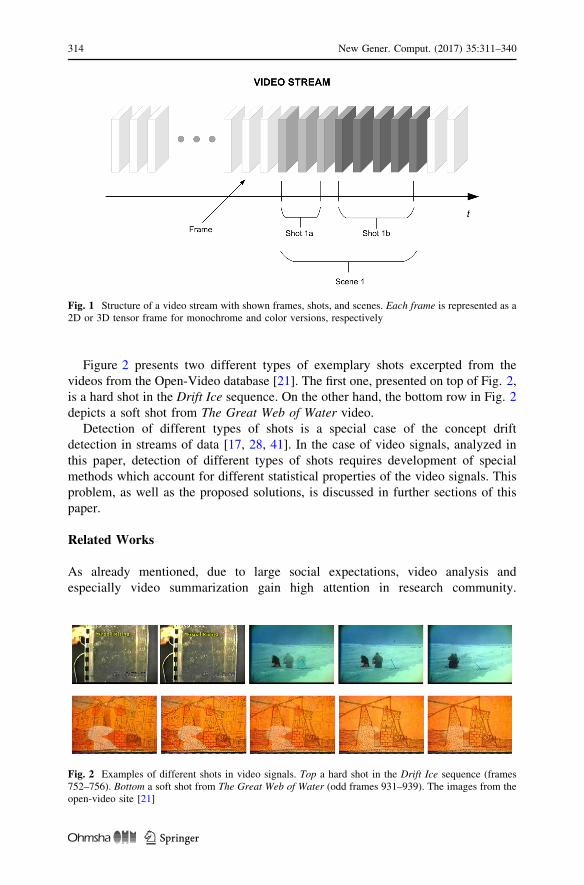
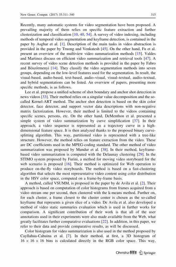
Figure 2 presents two different types of exemplary shots excerpted from the
videos from the Open-Video database [21]. The first one, presented on top of Fig. 2,
is a hard shot in the Drift Ice sequence. On the other hand, the bottom row in Fig. 2
depicts a soft shot from The Great Web of Water video.
Detection of different types of shots is a special case of the concept drift
detection in streams of data [17, 28, 41]. In the case of video signals, analyzed in
this paper, detection of different types of shots requires development of special
methods which account for different statistical properties of the video signals. This
problem, as well as the proposed solutions, is discussed in further sections of this
paper.
Related Works
As already mentioned, due to large social expectations, video analysis and
especially video summarization gain high attention in research community.
Fig. 1 Structure of a video stream with shown frames, shots, and scenes. Each frame is represented as a2D or 3D tensor frame for monochrome and color versions, respectively
Fig. 2 Examples of different shots in video signals. Top a hard shot in the Drift Ice sequence (frames752–756). Bottom a soft shot from The Great Web of Water (odd frames 931–939). The images from theopen-video site [21]
314 New Gener. Comput. (2017) 35:311–340
123
Recently, many automatic systems for video segmentation have been proposed. A
prevailing majority of them relies on specific feature extraction and further
clusterization and classification [10, 40, 54]. A survey of video indexing, including
methods of temporal video segmentation and keyframe detection, is contained in the
paper by Asghar et al. [1]. Description of the main tasks in video abstraction is
provided in the paper by Truong and Venkatesh [45]. On the other hand, Fu et al.
present an overview of the multiview video summarization methods [15]. Valdes
and Martinez discuss on efficient video summarization and retrieval tools [47]. A
recent survey of video scene detection methods is provided in the paper by Fabro
and Boszormenyi [14]. They classify the video segmentation methods into seven
groups, depending on the low-level features used for the segmentation. In result, the
visual-based, audio-based, text-based, audio–visual, visual–textual, audio–textual,
and hybrid segmentations can be listed. An overview of papers, presenting more
specific methods, is as follows.
Lee et al. propose a unified scheme of shot boundary and anchor shot detection in
news videos [33]. Their method relies on a singular value decomposition and the so-
called Kernel-ART method. The anchor shot detection is based on the skin color
detector, face detector, and support vector data descriptions with non-negative
matrix factorization. However, their method is limited to the videos containing
specific scenes, persons, etc. On the other hand, DeMenthon et al. presented a
simple system of video summarization by curve simplification [37]. In their
approach, a video sequence is represented as a trajectory curve in a high-
dimensional feature space. It is then analyzed thanks to the proposed binary curve-
splitting algorithm. This way, partitioned video is represented with a tree-like
structure. However, the method relies on feature extraction from the video. These
are DC coefficients used in the MPEG-coding standard. The other method of video
summarization was proposed by Mundur et al. [38]. In their method, keyframe-
based video summarization is computed with the Delaunay clustering [29]. In the
STIMO system proposed by Furini, a method for moving video storyboard for the
web scenario is proposed [16]. Their method is optimized for Web operation to
produce on-the-fly video storyboards. The method is based on a fast-clustering
algorithm that selects the most representative video content using color distribution
in the HSV color space, computed on a frame-by-frame basis.
A method, called VSUMM, is proposed in the paper by de Avila et al. [2]. Their
approach is based on computation of color histograms from frames acquired from a
video stream one per second, then clustered with the k-means method. Further on,
for each cluster, a frame closest to the cluster center is chosen as the so-called
keyframe that represents a given slice of a video. De Avila et al. also developed a
method of video static summaries evaluation which is used in further works for
comparison. A significant contribution of their work is that all of the user
annotations used in their experiments were also made available from the Web, what
greatly facilitates further comparative evaluations [22]. In addition, in this paper, we
refer to their data and provide comparative results, as will be discussed.
Color histogram for video summarization is also used in the method proposed by
Cayllahua-Cahuina et al. [7]. In their method, at first, a 3D histogram of
16 9 16 9 16 bins is calculated directly in the RGB color space. This way,
New Gener. Comput. (2017) 35:311–340 315
123
obtained vectors of 4096 elements are further processed with the PCA method for
compression. In the next step, the two clustering algorithms are employed. The first
Fuzzy-ART is responsible for determination of a number of clusters, while the
second Fuzzy C-Means perform frame clustering based on the color histogram
features. However, reported results indicate that using only color information is not
enough to obtain the satisfactory results [7].
In the paper by Medentzidou and Kotropoulos, a video summarization method
based on shot boundary detection with penalized contrast is proposed [36]. This
method also relies on color analysis, using the HSV color space, however. The mean
of the hue component is proposed as a way of change detection. Then, video
segments are extracted to capture video content. These are then described with a
linear model with the addition of noise. As reported, the method obtains results
comparable to other methods, such as [2].
The other video summarization method, called VSCAN, was proposed by
Mahmoud et al. [35]. Their method is based on a modified density-based spatial
clustering of applications with noise-clustering method (DBSCAN), which is used
to video summarization from color and texture features of each frame.
In our framework, we utilize tensor analysis. In the next section, we provide a
brief introduction to this domain, introducing notation and concepts necessary for
the understanding of the presented method. In the first row, the papers by de
Lathauwer et al. can be recommended [30–32]. Tensors and their decompositions
are also described in the papers by Kolda [27], Kolda and Bader [26], and also in the
books, for example, by Cichocki [6], or the one by Cyganek [10].
In this paper, we also rely on the concepts of the data stream analysis, concept
drift detection, as well as data classification in data streams. Recently, these gained
much attention among researchers. This new domain of data processing is analyzed,
for instance, in the book by Gama [17] or in the papers by Krawczyk et al. [28] or
Wozniak et al. [53], to name a few. The two domains—that is,streams of tensor
data—were pioneered by the works by Sun et al. [43, 44], as will be further
discussed.
Introduction to Tensors and Their Decompositions
In this section, we present the basics of visual signal representations with tensors, as
well as signal analysis based on tensor decompositions. Especially, tensor
decompositions gained much attention, since they lead to discovery of latent
factors, multidimensional data classification [9, 42] as well as for data compression
[52]. Among many, the most prominent is the higher order singular value
decomposition (HOSVD), canonical decomposition (Candecomp/Parafac)
[25, 26, 51], as well as the Tucker [46] and the best rank- (R1, R2,…, RP)
decomposition [10, 11, 30, 32]. The method presented in this paper relies on the
latter one, so its details as well as its computational aspects are discussed in further
sections of this paper.
316 New Gener. Comput. (2017) 35:311–340
123
Signal Processing with Tensors
Multidimensional measurements and signals are frequently encountered in science
and industry. Examples are multimedia, video surveillance, hyperspectral images,
sensor networks, to name a few. However, their processing with the standard vector-
based methods is usually not sufficient due to the loss of important information
contained in internal structure and relations among data. Thus, for analysis and
processing, more appropriate are methods that directly account for data dimen-
sionality. In this respect, it was shown that tensor-based methods frequently offer
many benefits, such as in the case of the tensorfaces, as well as view synthesis
proposed by Vasilescu and Terzopoulos [48–50], or data dimensionality reduction
by Wang and Ahuja [51, 52], handwritten digits recognition proposed by Savas and
Elden [42] or road signs recognition by Cyganek [9], to name a few. In this section,
we present a brief introduction to the tensor analysis necessary for understanding of
further parts of this paper. However, this short introduction by no means excerpts
the subject. Further information can be found in many publications, such as, for
instance, [5, 10, 11, 24, 25, 32, 48].
Let us now define a P-dimensional tensor as follows1:
A 2 <N1�N2�...NP ; ð1Þ
with each kth dimension denoted by Nk and for 1 B kBP. Regardless of its physical
meaning, a tensor can also be interpreted as a multidimensional cube of real-valued
data, in which each dimension corresponds to a different component or measure-
ment of the input data domain [10].
Based on the above definition, let us denote a jth vector (called a fiber) of a Pth-
order tensor A which is obtained by an exclusive change of one index nj
(1 B nj B Nj) while keeping all other indices fixed. A similar and very important
concept is a tensor flattening (also called – matricization [25]). For a Pth-order
tensor A, its jth flattening is defined as the following matrix:
A jð Þ 2 <Nj� N1N2...Nj�1Njþ1...NPð Þ: ð2Þ
A jth flattening is obtained from A after selecting a jth dimension, which
becomes a row index of A(j), whereas a product of all the rest indices constitutes a
column index of A(j). Columns of A(j) are called jth fibers of A, and they span a jth
tensor subspace.
A kth modal product T 9 kM of a tensor T 2 <N1�N2�...NP and a matrix M 2<Q�Nk is a tensor S 2 <N1�N2�...Nk�1�Q�Nkþ1�...NP , whose elements are expressed as
follows:
Sn1n2...nk�1qnkþ1...nP ¼ T �k Mð Þn1n2...nk�1qnkþ1...nP¼
XNk
nk¼1
tn1n2...nk�1nknkþ1...nPmqnk : ð3Þ
1 Tensors are denoted with the calligraphic letters, vectors and matrices are in bold face.
New Gener. Comput. (2017) 35:311–340 317
123
That is, Eq. (3) is an extension of the ‘‘classical’’ matrix multiplication, in which
the product involves multiplication of elements of the kth fibers of the tensor T and
consecutive rows of the matrix M. As a result, the jth dimension of T is changed to
Q [10, 30].
On the other hand and contrary to the well-known matrix algebra, there is no
single definition of a rank of a tensor. There are at least three different concepts of a
tensor rank from which the so-called rth rank will be used throughout this paper: An
rth rank of a tensor A is a dimension of the vector space spanned by the columns of
the rth flattening A(r) of this tensor.
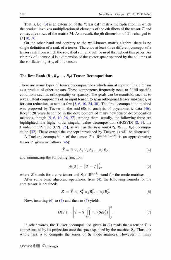
The Best Rank-(R1, R2, …, RP) Tensor Decompositions
There are many types of tensor decompositions which aim at representing a tensor
as a product of other tensors. These components frequently need to fulfill specific
conditions such as orthogonality or sparsity. The goals can be manifold, such as to
reveal latent components of an input tensor, to span orthogonal tensor subspaces, or
for data reduction, to name a few [5, 6, 10, 24, 30]. The first decomposition method
was proposed by Tucker in the mid-60s to analysis of psychometric data [46].
Recent 20 years benefited in the development of many new tensor decomposition
methods, though [5, 6, 10, 26, 27]. Among them, usually, the following three are
highlighted: the higher order singular value decomposition (HOSVD) [8, 9], the
Candecomp/Parafac (CP) [25], as well as the best rank-(R1, R2,…, RP) decompo-
sition [32]. These extend the concept introduced by Tucker, as will be discussed.
A Tucker decomposition of the tensor T 2 <N1�N2�...�NP is an approximating
tensor ~T given as follows [46]:
~T ¼ Z �1 S1 �2 S2. . .�P SP; ð4Þ
and minimizing the following function:
H Tð Þ ¼ T � ~T�� ��2
F; ð5Þ
where Z stands for a core tensor and Si 2 <Ni�Ri stand for the mode matrices.
After some basic algebraic operations, from (4), the following formula for the
core tensor is obtained:
Z ¼ ~T �1 ST1 �2 ST
2 . . .�P STP: ð6Þ
Now, inserting (6) to (4) and then to (5) yields
H Tð Þ ¼ T � TYP
k¼1
�k SkSTk
� ������
�����
2
F
: ð7Þ
In other words, the Tucker decomposition given in (7) reads that a tensor T is
approximated by its projection onto the space spanned by the matrices Sk. Thus, the
whole task is to compute the series of Sk mode matrices. However, in many
318 New Gener. Comput. (2017) 35:311–340
123
applications, it is beneficial to request in (4) orthogonality or specific ranks of Sk. If
such a constraint is assumed, then the Tucker decomposition (4) leads to the best
rank-(R1, R2,…, RP) decomposition, defined as follows [32].
The best rank-(R1, R2,…, RP) approximation of a tensor T 2 <N1�N2�...�NP is a
tensor ~T of ranks in each of its modes rank1~T ¼ R1, rank2
~T ¼ R2,…,
rankP ~T ¼ RP, respectively, which minimizes the function (7).
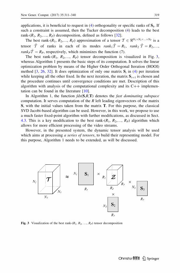
The best rank-(R1, R2,…, RP) tensor decomposition is visualized in Fig. 3,
whereas Algorithm 1 presents the basic steps of its computation. It solves the linear
optimization problem by means of the Higher Order Orthogonal Iteration (HOOI)
method [3, 26, 32]. It does optimization of only one matrix Si in (4) per iteration
while keeping all the other fixed. In the next iteration, the matrix Si?1 is chosen and
the procedure continues until convergence conditions are met. Description of this
algorithm with analysis of the computational complexity and its C?? implemen-
tation can be found in the literature [10].
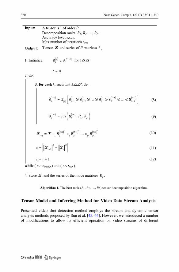
In Algorithm 1, the function fds(S,R,T) denotes the fast dominating subspace
computation. It serves computation of the R left leading eigenvectors of the matrix
S, with the initial values taken from the matrix T. For this purpose, the classical
SVD Jacobi-based algorithm can be used. However, in this work, we propose to use
a much faster fixed-point algorithm with further modifications, as discussed in Sect.
4.3. This is a key modification to the best rank-(R1, R2,…, RP) algorithm which
allows for more efficient processing of the video streams.
However, in the presented system, the dynamic tensor analysis will be used
which aims at processing a series of tensors, to build their representing model. For
this purpose, Algorithm 1 needs to be extended, as will be discussed.
Fig. 3 Visualization of the best rank-(R1, R2, …, RP) tensor decomposition
New Gener. Comput. (2017) 35:311–340 319
123
Tensor Model and Inferring Method for Video Data Stream Analysis
Presented video shot detection method employs the stream and dynamic tensor
analysis methods proposed by Sun et al. [43, 44]. However, we introduced a number
of modifications to allow its efficient operation on video streams of different
320 New Gener. Comput. (2017) 35:311–340
123
dimensions, as well as a new method of construction of a tensor model specific to
the video signals. In this section, we describe the basic ideas behind the tensor
stream processing framework, as well as our proposed features which allow efficient
video shot detection in various types of video streams.
System Architecture and Basic Concepts of the Tensor Stream Analysis
In the proposed system, a stream of input tensor data of the same order P is
assumed. As already mentioned, in this version, we do not assume any feature
extraction from the input tensors. This means that any type of signal can be applied
to the presented algorithms. Thus, the method works fine with both the monochrome
as well as color video streams. This makes the proposed method versatile.
Nevertheless, if there is additional knowledge of a signal type, then methods that
compute specific features can be more discriminative but only for this specific type
of a signal. This happens with color histograms, frequently used in video shot
detection [2, 7, 35]. Such methods will not work with monochrome or hyperspectral
images, though. Thus, in our framework, features can also be included in the input
tensors to make the signals more discriminative, but this possibility is left for further
research. To proceed, we introduce a number of definition after the work of Sun
et al. [44]: a sequence of tensors is a series of m tenors Ai, where 1 B i B m, each of
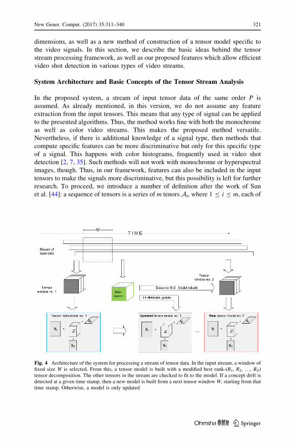
Fig. 4 Architecture of the system for processing a stream of tensor data. In the input stream, a window offixed size W is selected. From this, a tensor model is built with a modified best rank-(R1, R2, …, RP)tensor decomposition. The other tensors in the stream are checked to fit to the model. If a concept drift isdetected at a given time stamp, then a new model is built from a next tensor window W, starting from thattime stamp. Otherwise, a model is only updated
New Gener. Comput. (2017) 35:311–340 321
123
Pth-order A 2 <N1�N2�...NP , and assuming that m is constant. A stream of tensors is a
sequence of m tensors, where m is a natural value increasing with time.
Our proposed system operates as follows. From the input stream of tensor data, a
window of consecutive frame tensors of size W is selected. All of them are used to
build a best rank-(R1, R2,…, RP) tensor model, as described in Algorithm 1.
However, the main modification of this model, which we incorporate after the work
by Sun et al., consists of computing a covariance matrix out of all flattened versions
of the tensors from the selected window W. This way, for each of the P flattenings, a
single covariance matrix is created from all tensors in the input window. Thus, such
a covariance matrix conveys statistical information on all of the input tensors in a
given flattening mode. The next computational perk of this approach is that the
covariance matrix is a positive definite one for which a more effective eigenvalue
decomposition method could be applied, as will be discussed. It is worth noticing
that such an approach differs from the building and decomposing of a new large
tensor composed of all tensors from the window stream after adding a new
dimension NP?1 of value W. Details of the modified best rank-(R1, R2,…, RP)
decomposition, as well as of the model build-and-update procedures from the
streams of tensor data are presented in the next section.
Figure 4 shows architecture of the system for processing a stream of tensor data.
As already mentioned, in the input stream, a window of fixed size W is selected.
From this, a tensor model is built with a modified best rank-(R1, R2,…, RP) tensor
decomposition. The other tensors in the stream are checked if they fit to the model
form the latest window W based on a special fitness function, as will be discussed. If
a concept drift in the stream is detected, then a new model is built from a next tensor
window W at the given time stamp. Otherwise, the model needs only to be updated
to account for the new tensor. This is the model adaptation mechanism. Both the
model build-and-update algorithms are described in the next sections.
A Modified Best Rank-(R1, R2,…, RP) Tensor Decomposition for StreamTensors
Algorithm 2 presents the best rank-(R1, R2,…, RP) tensor decomposition algorithm
modified for processing of a stream of tensor data.
322 New Gener. Comput. (2017) 35:311–340
123
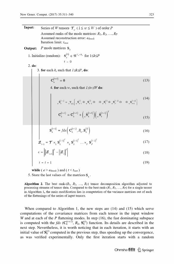
When compared to Algorithm 1, the new steps are (14) and (15) which serve
computations of the covariance matrices from each tensor in the input window
W and at each of the P flattening modes. In step (16), the fast dominating subspace
is computed with the fds (Ck(t?1), Rk, Sk
(t)) function. Its details are described in the
next step. Nevertheless, it is worth noticing that in each iteration, it starts with an
initial value of Sk(t) computed in the previous step, thus speeding up the convergence,
as was verified experimentally. Only the first iteration starts with a random
New Gener. Comput. (2017) 35:311–340 323
123
initialization. It is important to notice that the two loops in Algorithm 2 determine
the speed of a model build and, in consequence, computation of the whole method.
As already mentioned, after building the model from the input tensor stream, the
incoming tensor data are checked to fit that model. Therefore, a suitable fitness
function needs to be developed. This, in the context of video stream analysis, will be
discussed in the next section. If a new tensor does not fit to the model, it needs to be
rebuilt from scratch, starting at the position in the stream of a just checked tensor.
On the other hand, if it fits, then the model also needs to be rebuilt to account for this
new tensor and to adjust to the changes in the stream. However, despite the speed-up
of the model build procedure presented in Algorithm 2 its continuous re-
computation at each tensor in the stream is computationally not tractable.
Therefore, instead, a mode update procedure is employed, as proposed by Sun
et al. [43]. It simply relies on an update of the covariance matrices in (15) in
Algorithm 2 in each of the flattening modes with the new tensor data. Such a
procedure is well known in the statistics and relies on the following computation:
Ctþ1k ¼ aCt
k þ Stþ1k Stþ1T
k ; ð20Þ
where a is a forgetting factor of a previous model, and Sk(t?1) is a kth mode matrix of
a new (updating) tensor at a time step t?1. Summing up, the described method
assumes model build from which only the covariance mode matrices need to be
stored. Thus, the input tensors from the window W are not accessed anymore which
results in significant memory savings. Then, on a new tensor, if decided to update
the model, for each of the flattening modes, the proper covariance matrices of a
model are updated in accordance with (20). Finally, fds (Ck(t?1), Rk, Sk
(t)) from the
step (16) in Algorithm 2, needs to be computed, but only once. However, it should
be pointed out that the covariance matrix update rule (15), as well as (20), holds
under assumption of the same mean value among data. If this is not true, then to
keep the model accurate enough, also the mean updating component should be
added to the aforementioned equations [34]. Nevertheless, we also follow this
simplifying assumption and use the updating model (20). This is justified by the fact
that we are interested in detecting signal changes which, if happen, usually also lead
to a change of the mean values in data. In such a case, the model will not hold
anymore which will trigger its rebuild process, as discussed in Sect. 4.5, and the shot
will be detected.
Efficient Computation of the Dominating Tensor Subspace
Application of the tensor decomposition to analysis of tensor streams, such as video
signals, would be very limited or even useless if cannot be efficiently computed. In
this respect, the best would be to have a real-time response or at least an answer in a
user acceptable time, which certainly is a subjective notion. To be more concrete,
we measure processing time in terms of the input (tensor) frame processing.
However, efficiency means also computational stability, as will be discussed.
324 New Gener. Comput. (2017) 35:311–340
123
As already mentioned, thanks to the formulation of computation steps in
Algorithm 2 with only the positive real symmetric matrices, it is possible to employ
a faster algorithm than the SVD decomposition of matrices for a general case. For
this purpose, in our system, the so-called fixed-point eigen decomposition algorithm
is used for computation of the fds function from the step (16) in Algorithm 2. This
method was first proposed to be used in tensor decomposition by Muti and
Bourennane [39]. Then, it was also used for computation of the HOSVD tensor
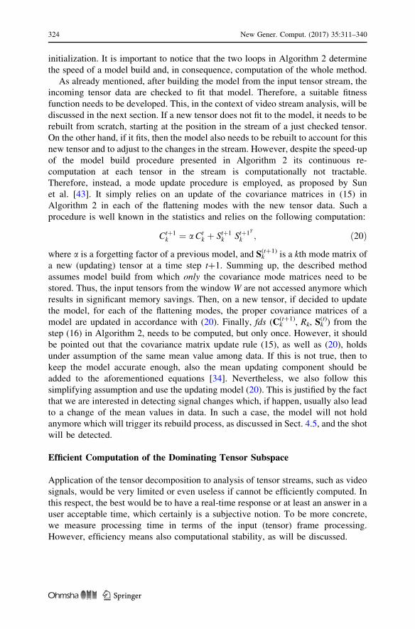
decomposition in the work by Cyganek and Wozniak [12]. Algorithm 3 shows the
key steps of this method.
However, after longer use of this algorithm for different tensor decompositions,
we noticed its problems with its numerical stability. Under closer examination, it
New Gener. Comput. (2017) 35:311–340 325
123
appeared that the problem is usually caused by the multiplication step (21) in
Algorithm 3, especially if elements of the input matrix C have magnitudes few order
of magnitude higher than values of the vector ek. Therefore, our proposition is to
add an additional normalization step (22) just after the multiplication (21) and
before the Gram–Schmidt orthogonalization step (23). Our experiments showed that
the proposed modification improved the numerical stability of the whole procedure
with insignificant additional computations.
The next modification proposed in this paper is an automatic mechanism of
evaluating the number of important eigenvalues kimp, which is determined
dynamically during the run of the algorithm. The main idea consists in checking
a ratio of logarithms of the eigenvalues, corresponding to the consecutive
eigenvectors, respectively. If this ratio exceeds a preset threshold, in our
experiments set to 1.5, then the procedure is stopped. In practice, this simple rule
allows for significant computational savings.
The next simple modification is initialization of the starting values of the
eigenvectors with these values computed in the previous iteration, rather than
initialization with random values, as presented in (16). This relies on a simple
observation that the computed eigenvectors do not lie far from each other between
consecutive iterations. Therefore, such initialization, usually, leads to the faster
convergence than when started from the randomly chosen initial values. Random
initialization is applied only at the first run.
Concept Drift Detection in Video Tensor Streams
The goal of the concept drift detection is to discover conditions in which a data
model is not sufficient to well represent content of the current data stream. This
usually happens due to changes of the statistical properties of the data stream caused
by external factors. The concept drift detection in different streams belongs to a
dynamical research area [17, 18, 28]. In the case of video streams, a concept drift
usually corresponds to content change in video signal due to a hard or soft shots, as
already discussed.
In the proposed system, the data model is obtained with the best rank-(R1,
R2,…,RP) tensor decomposition, as already described. The model is stored as a
series of matrices Sk and the variance matrices Ck. Then, a model fit measure for a
new tensor X is indirectly obtained from the error value (7). However, we need to
develop a measure of checking if a new tensor X fits to the model.
The simplest way to build a fitness algorithm is first, to check consistency of a
model and then relate the model consistency to the fit measure of an unknown tensor
data X . This can be done by computing all values of H(T i) in (7), for all T i
belonging to the window W. Then, their mean and standard deviation can be used to
describe the model [43]. These are simply given as follows:
�H ¼ 1
#W
Xw
i¼1
Hi; ð26Þ
and
326 New Gener. Comput. (2017) 35:311–340
123
r2 ¼ 1
#W � 1
Xw
i¼1
Hi � �Hð Þ2; ð27Þ
where #W denotes a number of tensors in the window W. Finally, a new tensor, X ,
can be checked to fit to the model by a simple ± 3r rule as follows:
HX � �H�� ��\ 3 r: ð28Þ
However, after examining this simple model on a number of video streams, we
noticed that, instead of the absolute error values H, better results are obtained if the
differences DH of H are used. The error function difference is defined simply as
DHi � Hi�1 �Hi: ð29Þ
Finally, the fitness measure has to be further modified to account for the series of
tensor frames which change insignificantly or do not change at all. This happens, for
instance, for the series of frames from a video with no content change. In such cases,
the r parameter tends toward 0, and in a result, even not significant change in a new
frame would not fulfill in accordance with (28), and in a consequence, the entirely
new model rebuild process would be launched, which is not justified and
computational costly. Thus, to account for such situations, our fitness measure is
expressed as follows:
DHX � �HD
�� ��\ a rD þ b; ð30Þ
where �HD and rD are the mean and standard deviation computed from the differ-
ences of consecutive fit values in (29), respectively, a is multiplicative factor (set in
our experiments to the range 1.5–3.7), and b is an additive constant (in our
experiments set to 0.2–2.5).
Video Tensor Stream Model Build-and-Update Scheme
All of the aforementioned mechanisms are assembled here into a complete tensor-
based method for efficient video stream analysis. Algorithm 4 shows our proposed
tensor model build and concept drift detection mechanisms for video stream
analysis.
It is worth noticing that the initial rank values R1, R2,…,RP are the maximal
possible ranks that are considered when building the model. However, real ranks are
determined based on the already described automatic rank assessment mechanism
and, in practice, are usually much smaller than the conservatively assumed initial
ranks. In our experiments, these are set as a percentage of the dimensions of the
tensor frames. For instance, these are R1 = 0.25N1, R2 = 0.25N2, and R3 = N3,
where N1 and N2 stand for the column and row dimensions, whereas N3 for the color
one, respectively.
The next stabilizing mechanism introduced in our system is a counter of
consecutive frames that do not fit the current tensor model. If the model is not
fulfilled for all consecutive G frames, then only the total model rebuild procedure is
New Gener. Comput. (2017) 35:311–340 327
123
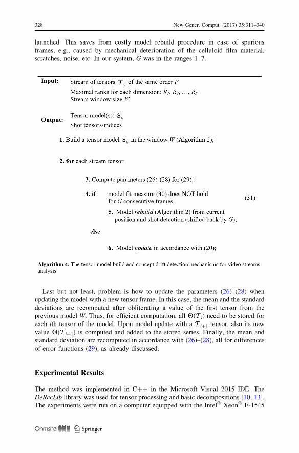
launched. This saves from costly model rebuild procedure in case of spurious
frames, e.g., caused by mechanical deterioration of the celluloid film material,
scratches, noise, etc. In our system, G was in the ranges 1–7.
Last but not least, problem is how to update the parameters (26)–(28) when
updating the model with a new tensor frame. In this case, the mean and the standard
deviations are recomputed after obliterating a value of the first tensor from the
previous model W. Thus, for efficient computation, all H(T i) need to be stored for
each ith tensor of the model. Upon model update with a T i?1 tensor, also its new
value H(T i?1) is computed and added to the stored series. Finally, the mean and
standard deviation are recomputed in accordance with (26)–(28), all for differences
of error functions (29), as already discussed.
Experimental Results
The method was implemented in C?? in the Microsoft Visual 2015 IDE. The
DeRecLib library was used for tensor processing and basic decompositions [10, 13].
The experiments were run on a computer equipped with the Intel� Xeon� E-1545
328 New Gener. Comput. (2017) 35:311–340
123
processor operating at 2.9 GHz, with 64 GB RAM, and 64-bit version of Windows
10.
For evaluation, we used the VSUMM database and provided therein summa-
rization of different videos [2, 22]. Such an approach has been undertaken by many
researchers and allows qualitative evaluation and comparison among a group of
video summarization methods. This database contains 50 videos from the Open-
Video Project [21]. The videos are stored in the MPEG-1 format with 30 fps and
resolution 352 9 240 pixels, color and sound, with duration in the range of
1–4 min. They are classified into different genres, such as documentary,
educational, ephemeral, historical, and lecture.
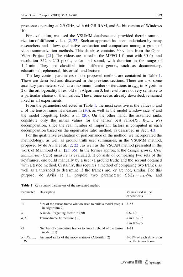
The key control parameters of the proposed method are contained in Table 1.
These are described and discussed in the previous sections. There are also some
auxiliary parameters, such as a maximum number of iterations in tmax in Algorithm
2 or the orthogonality threshold e in Algorithm 3, but results are not very sensitive to
a particular choice of their values. These, once set as already described, remained
fixed in all experiments.
From the parameters collected in Table 1, the most sensitive is the values a and
b of the tensor frame fit measure in (30), as well as the model window size W and
the model forgetting factor a in (20). On the other hand, the assumed ranks
constitute only the initial values for the tensor best rank-(R1, R2,…, RP)
decomposition, since the real number of important factors is computed in each
decomposition based on the eigenvalue ratio method, as described in Sect. 4.3.
For the qualitative evaluation of performance of the method, we incorporated the
methodology, as well as ground truth user summaries, in the VSUMM method,
proposed by de Avila et al. [2, 22], as well as the VSCAN method presented in the
work of Mahmoud et al. [23, 35]. In the former approach, the Comparison of User
Summaries (CUS) measure is evaluated. It consists of comparing two sets of the
keyframes, one build manually by a user (a ground truth) and the second obtained
with a tested method. Certainly, this requires a method of comparing two frames, as
well as a threshold to determine if the frames are, or are not, similar. For this
purpose, de Avila et al. propose two parameters: CUSA = nAU/nU and
Table 1 Key control parameters of the presented method
Parameter Description Values used in the
experiments
W Size of the tensor-frame window used to build a model (step 4
in Algorithm 2)
3–55
a A model forgetting factor in (20) 0.6–1.0
a, b Tensor-frame fit measure (30) a in 1.5–3.7
b in 0.2–2.5
G Number of consecutive frames to launch rebuild of the tensor
model (31)
1–11
R1, R2, …,
RP
Assumed ranks of the mode matrices (Algorithm 2) 5–75% of each dimension
of the tensor frame
New Gener. Comput. (2017) 35:311–340 329
123
CUSE = *nAU/nU, where nAU denotes a number of matching keyframes from the
automatic summary (AS) and the user-annotated summary, *nAU is the complement
of this set (i.e., the frames that were not matched), whereas nU is a total number of
keyframes from the user summary only (US). However, as presented by Mahmoud
et al., more informative parameters are precision P and recall R, since they also
convey information on the keyframes present in AS and not present in US or vice
versa. As a trade-off of the two, the so-called F measure is used [20, 35, 45]. Thus,
in our experiments, we used the measures defined as follows:
P ¼ nAU
nA; R ¼ nAU
nU; F ¼ 2
PR
Pþ R; ð32Þ
where nAU denotes a number of keyframes from the automatic summary that match
the ones from the user’s summary, and nA is a number of total keyframes from the
automatic summary only while nU from the user’s summary.
As already mentioned, the comparisons are done between the found shots and the
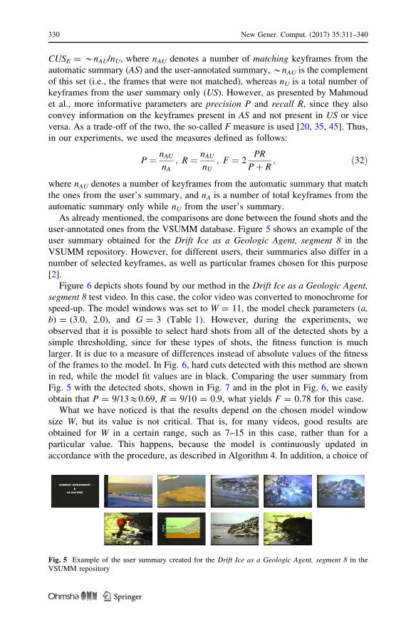
user-annotated ones from the VSUMM database. Figure 5 shows an example of the
user summary obtained for the Drift Ice as a Geologic Agent, segment 8 in the
VSUMM repository. However, for different users, their summaries also differ in a
number of selected keyframes, as well as particular frames chosen for this purpose
[2].
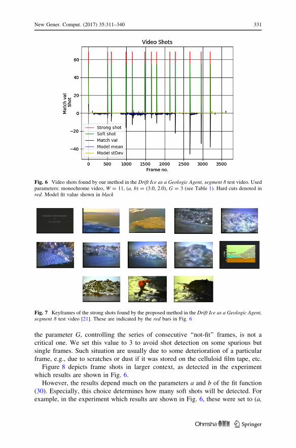
Figure 6 depicts shots found by our method in the Drift Ice as a Geologic Agent,
segment 8 test video. In this case, the color video was converted to monochrome for
speed-up. The model windows was set to W = 11, the model check parameters (a,
b) = (3.0, 2.0), and G = 3 (Table 1). However, during the experiments, we
observed that it is possible to select hard shots from all of the detected shots by a
simple thresholding, since for these types of shots, the fitness function is much
larger. It is due to a measure of differences instead of absolute values of the fitness
of the frames to the model. In Fig. 6, hard cuts detected with this method are shown
in red, while the model fit values are in black. Comparing the user summary from
Fig. 5 with the detected shots, shown in Fig. 7 and in the plot in Fig. 6, we easily
obtain that P = 9/13&0.69, R = 9/10 = 0.9, what yields F = 0.78 for this case.
What we have noticed is that the results depend on the chosen model window
size W, but its value is not critical. That is, for many videos, good results are
obtained for W in a certain range, such as 7–15 in this case, rather than for a
particular value. This happens, because the model is continuously updated in
accordance with the procedure, as described in Algorithm 4. In addition, a choice of
Fig. 5 Example of the user summary created for the Drift Ice as a Geologic Agent, segment 8 in theVSUMM repository
330 New Gener. Comput. (2017) 35:311–340
123
the parameter G, controlling the series of consecutive ‘‘not-fit’’ frames, is not a
critical one. We set this value to 3 to avoid shot detection on some spurious but
single frames. Such situation are usually due to some deterioration of a particular
frame, e.g., due to scratches or dust if it was stored on the celluloid film tape, etc.
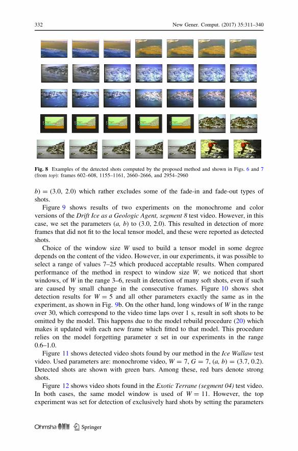
Figure 8 depicts frame shots in larger context, as detected in the experiment
which results are shown in Fig. 6.
However, the results depend much on the parameters a and b of the fit function
(30). Especially, this choice determines how many soft shots will be detected. For
example, in the experiment which results are shown in Fig. 6, these were set to (a,
Fig. 6 Video shots found by our method in the Drift Ice as a Geologic Agent, segment 8 test video. Usedparameters: monochrome video, W = 11, (a, b) = (3.0, 2.0), G = 3 (see Table 1). Hard cuts denoted inred. Model fit value shown in black
Fig. 7 Keyframes of the strong shots found by the proposed method in the Drift Ice as a Geologic Agent,segment 8 test video [21]. These are indicated by the red bars in Fig. 6
New Gener. Comput. (2017) 35:311–340 331
123
b) = (3.0, 2.0) which rather excludes some of the fade-in and fade-out types of
shots.
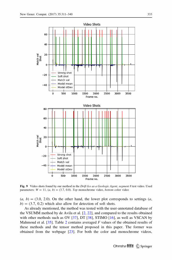
Figure 9 shows results of two experiments on the monochrome and color
versions of the Drift Ice as a Geologic Agent, segment 8 test video. However, in this
case, we set the parameters (a, b) to (3.0, 2.0). This resulted in detection of more
frames that did not fit to the local tensor model, and these were reported as detected
shots.
Choice of the window size W used to build a tensor model in some degree
depends on the content of the video. However, in our experiments, it was possible to
select a range of values 7–25 which produced acceptable results. When compared
performance of the method in respect to window size W, we noticed that short
windows, of W in the range 3–6, result in detection of many soft shots, even if such
are caused by small change in the consecutive frames. Figure 10 shows shot
detection results for W = 5 and all other parameters exactly the same as in the
experiment, as shown in Fig. 9b. On the other hand, long windows of W in the range
over 30, which correspond to the video time laps over 1 s, result in soft shots to be
omitted by the model. This happens due to the model rebuild procedure (20) which
makes it updated with each new frame which fitted to that model. This procedure
relies on the model forgetting parameter a set in our experiments in the range
0.6–1.0.
Figure 11 shows detected video shots found by our method in the Ice Wallaw test
video. Used parameters are: monochrome video, W = 7, G = 7, (a, b) = (3.7, 0.2).
Detected shots are shown with green bars. Among these, red bars denote strong
shots.
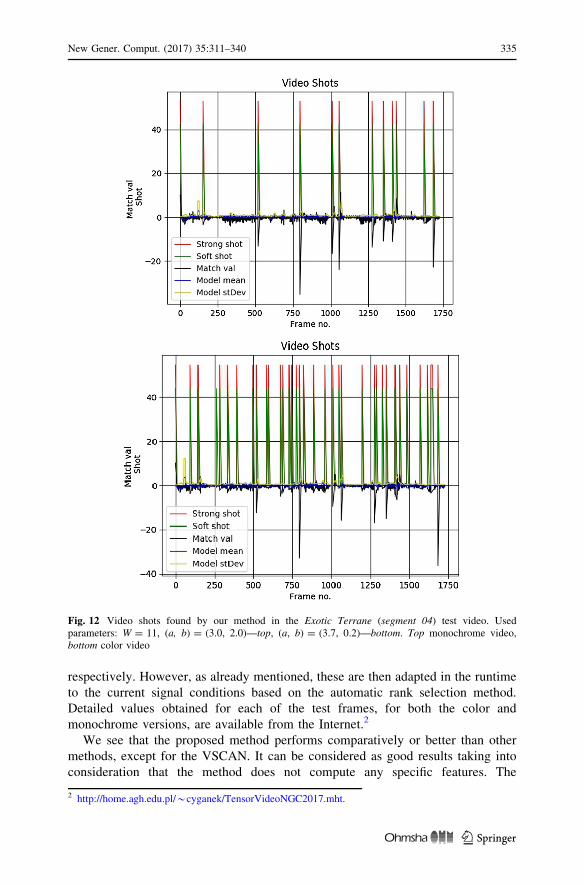
Figure 12 shows video shots found in the Exotic Terrane (segment 04) test video.
In both cases, the same model window is used of W = 11. However, the top
experiment was set for detection of exclusively hard shots by setting the parameters
Fig. 8 Examples of the detected shots computed by the proposed method and shown in Figs. 6 and 7(from top): frames 602–608, 1155–1161, 2660–2666, and 2954–2960
332 New Gener. Comput. (2017) 35:311–340
123
(a, b) = (3.0, 2.0). On the other hand, the lower plot corresponds to settings (a,
b) = (3.7, 0.2) which also allow for detection of soft shots.
As already mentioned, the method was tested with the user-annotated database of
the VSUMM method by de Avila et al. [2, 22], and compared to the results obtained
with other methods such as OV [37], DT [38], STIMO [16], as well as VSCAN by
Mahmoud et al. [35]. Table 2 contains averaged F values of the obtained results of
these methods and the tensor method proposed in this paper. The former was
obtained from the webpage [23]. For both the color and monochrome videos,
Fig. 9 Video shots found by our method in the Drift Ice as a Geologic Agent, segment 8 test video. Usedparameters: W = 11, (a, b) = (3.7, 0.8). Top monochrome video, bottom color video
New Gener. Comput. (2017) 35:311–340 333
123
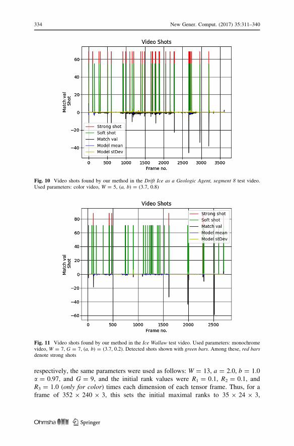
respectively, the same parameters were used as follows: W = 13, a = 2.0, b = 1.0
a = 0.97, and G = 9, and the initial rank values were R1 = 0.1, R2 = 0.1, and
R3 = 1.0 (only for color) times each dimension of each tensor frame. Thus, for a
frame of 352 9 240 9 3, this sets the initial maximal ranks to 35 9 24 9 3,
Fig. 10 Video shots found by our method in the Drift Ice as a Geologic Agent, segment 8 test video.Used parameters: color video, W = 5, (a, b) = (3.7, 0.8)
Fig. 11 Video shots found by our method in the Ice Wallaw test video. Used parameters: monochromevideo, W = 7, G = 7, (a, b) = (3.7, 0.2). Detected shots shown with green bars. Among these, red barsdenote strong shots
334 New Gener. Comput. (2017) 35:311–340
123
respectively. However, as already mentioned, these are then adapted in the runtime
to the current signal conditions based on the automatic rank selection method.
Detailed values obtained for each of the test frames, for both the color and
monochrome versions, are available from the Internet.2
We see that the proposed method performs comparatively or better than other
methods, except for the VSCAN. It can be considered as good results taking into
consideration that the method does not compute any specific features. The
2 http://home.agh.edu.pl/*cyganek/TensorVideoNGC2017.mht.
Fig. 12 Video shots found by our method in the Exotic Terrane (segment 04) test video. Usedparameters: W = 11, (a, b) = (3.0, 2.0)—top, (a, b) = (3.7, 0.2)—bottom. Top monochrome video,bottom color video
New Gener. Comput. (2017) 35:311–340 335
123
experiments showed that a difference between the color and monochrome video is
about 0.03. After closer analysis, we noticed that using color leads to removal of
some of the false positives. Nevertheless, the difference in accuracy between the
color and monochrome versions is not too big, which can be explained by a small
value of the color dimension, that is three, as well as by a correlation between the
color channels. On the other hand, VSUMM and VSCAN rely on color histograms.
This means that the proposed method can work with the monochrome videos,
whereas the former cannot. In addition, the proposed method can almost
automatically accommodate another dimensions, such as in the case of multiview
or hyperspectral streams. When analyzing results of operation of the proposed
method on various test video streams, we observed that frequently, it tends to detect
more shots than in the user-annotated surveys used for methods evaluation (false
positives). This depends strongly on the chosen parameters, especially the ones
controlling the frame fitness measure, as was discussed. Nevertheless, detected shots
can also be considered as valid, since usually, there is a noticeable change of frame
contents, as can be observed. However, such operation results in high recall
parameter but rather poor precision at the same time, what explains results, as
presented in Table 2.
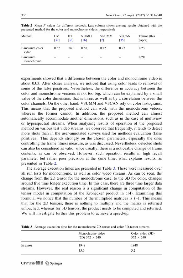
The average execution times are presented in Table 3. These were measured over
all run tests for monochrome, as well as color video streams. As can be seen, the
change from the 2D tensor for the monochrome case, to the 3D for color, changes
around five time longer execution time. In this case, there are three time larger data
streams. However, the real reason is a significant change in computation of the
tensor model in computation of the Kronecker product in (14). Examining this
formula, we notice that the number of the multiplied matrices is P-1. This means
that for the 2D tensors, there is nothing to multiply and the matrix is returned
untouched, whereas for 3D tensors, the product needs to be computed and returned.
We will investigate further this problem to achieve a speed-up.
Table 2 Mean F values for different methods. Last column shows average results obtained with the
presented method for the color and monochrome videos, respectively
Method OV
[37]
DT
[38]
STIMO
[16]
VSUMM
[2]
VSCAN
[35]
Tensor (this
paper)
F-measure color
video
0.67 0.61 0.65 0.72 0.77 0.73
F-measure
monochrome
– – – – – 0.70
Table 3 Average execution time for the monochrome 2D-tensor and color 3D-tensor streams
Monochrome video
(2D) 352 9 240
Color video (3D)
352 9 240
Frames 1948 1948
15.6 3.2
336 New Gener. Comput. (2017) 35:311–340
123
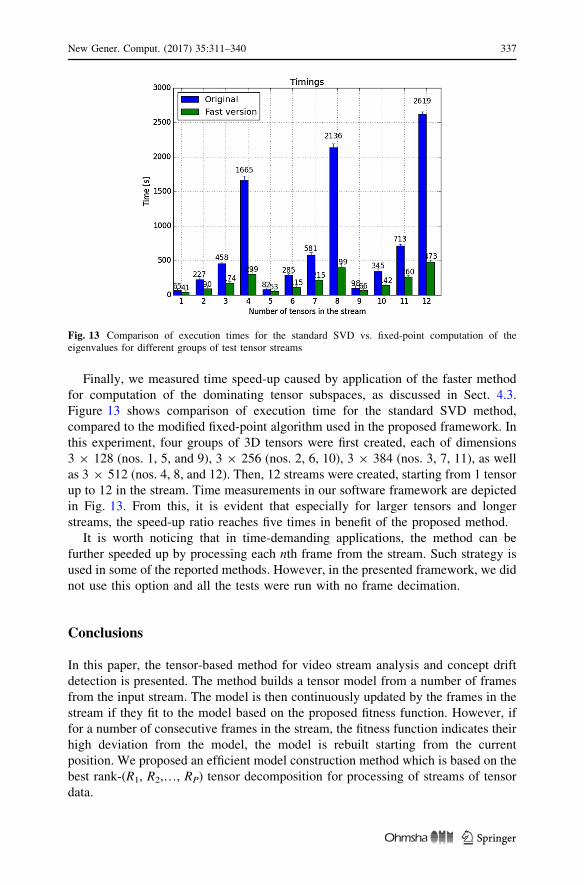
Finally, we measured time speed-up caused by application of the faster method
for computation of the dominating tensor subspaces, as discussed in Sect. 4.3.
Figure 13 shows comparison of execution time for the standard SVD method,
compared to the modified fixed-point algorithm used in the proposed framework. In
this experiment, four groups of 3D tensors were first created, each of dimensions
3 9 128 (nos. 1, 5, and 9), 3 9 256 (nos. 2, 6, 10), 3 9 384 (nos. 3, 7, 11), as well
as 3 9 512 (nos. 4, 8, and 12). Then, 12 streams were created, starting from 1 tensor
up to 12 in the stream. Time measurements in our software framework are depicted
in Fig. 13. From this, it is evident that especially for larger tensors and longer
streams, the speed-up ratio reaches five times in benefit of the proposed method.
It is worth noticing that in time-demanding applications, the method can be
further speeded up by processing each nth frame from the stream. Such strategy is
used in some of the reported methods. However, in the presented framework, we did
not use this option and all the tests were run with no frame decimation.
Conclusions
In this paper, the tensor-based method for video stream analysis and concept drift
detection is presented. The method builds a tensor model from a number of frames
from the input stream. The model is then continuously updated by the frames in the
stream if they fit to the model based on the proposed fitness function. However, if
for a number of consecutive frames in the stream, the fitness function indicates their
high deviation from the model, the model is rebuilt starting from the current
position. We proposed an efficient model construction method which is based on the
best rank-(R1, R2,…, RP) tensor decomposition for processing of streams of tensor
data.
Fig. 13 Comparison of execution times for the standard SVD vs. fixed-point computation of theeigenvalues for different groups of test tensor streams
New Gener. Comput. (2017) 35:311–340 337
123
The method was built and tested in the framework of video stream processing for
detection of the video shots. The main benefit of using the tensor representation and
decomposition is their natural ability to account for many internal dimensions of the
frames constituting a video stream as well as its ability to operate with original
signals with no necessity of feature detection. This can be beneficial in the case of
multidimensional signals or measurements coming in a stream and for which their
statistical properties are not known a priori. Nevertheless, features can be easily
incorporated as the next dimensions of the input tensors. However, each additional
dimension incurs a polynomial grow of the computational complexity, as well as
memory consumption. The analysis of tensors joining signal and/or additional signal
features is left for further research.
The method was adjusted to work with color and monochrome videos by
designing a specific concept drift detector. The method was then tested on the Open-
Video database with monochrome and color versions of the test videos. For both
types, the achieved accuracy can be compared favorably with majority of the video
keyframe detection methods, especially designed to process exclusively color
videos. Hence, the proposed tensor method has the ability to work with any type of
video signals, such as the monochrome, color, hyperspectral, etc. with no a priori
assumption on specific statistical properties of signals. On the other hand, we
noticed relatively poor recognition of specific types of the soft temporal signal
changes. This happens because if a change is not sufficiently abrupt to cause model
rebuild, the adaptively progressing model gets gradually adapted to the slow/soft
signal changes. However, these can be monitored by, e.g., higher standard deviation
of the fit measure, although its level depends on the signal type. In addition, a better
concept drift detector method can be designed which is also left for future research.
Nevertheless, the method requires significant memory and computational
resources. To improve its performance, the fast method of dominant tensor
subspace construction is proposed. Thanks to this, a significant speed-up ratio was
obtained when compared to the standard eigen problem solution based on the SVD
decomposition. The tensor subspace method was further modified, as proposed in
this paper, to increase its numerical stability and to allow for automatic
determination of the dominating eigenvalues.
Further research will be oriented toward improvement of accuracy and speed of
the proposed method, possibly by developing more efficient model fitness functions,
as well as by development of parallel tensor decomposition methods.
Acknowledgements This work was supported by the Polish National Science Center NCN under the
Grant No. 2014/15/B/ST6/00609. This work was supported by the statutory funds of the Department of
Systems and Computer Networks, Faculty of Electronics, Wroclaw University of Science and
Technology.
Open Access This article is distributed under the terms of the Creative Commons Attribution 4.0
International License (http://creativecommons.org/licenses/by/4.0/), which permits unrestricted use, dis-
tribution, and reproduction in any medium, provided you give appropriate credit to the original
author(s) and the source, provide a link to the Creative Commons license, and indicate if changes were
made.
338 New Gener. Comput. (2017) 35:311–340
123
References
1. Asghar, M.N., Hussain, F., Manton, R.: Video indexing: a survey. Int. J. Comput. Inf. Technol.
03(01), 148–169 (2014)
2. de Avila, S.E.F., Lopes, A.P.B., da Luz Jr., A., Araujo, A.A.: VSUMM: a mechanism designed to
produce static video summaries and a novel evaluation method. Pattern Recogn. Lett. 32, 56–68 (2011)
3. Bader, B.W., Kolda, T. G.: Algorithm 862: MATLAB tensor classes for fast algorithm prototyping.
ACM Trans. Math. Softw. 32(4), 635–653 (2006)
4. Bellman, R.E.: Adaptive control processes: a guided tour. Princeton University, Princeton (1961)
5. Cichocki, A., Zdunek, R., Amari, S.: Nonnegative matrix and tensor factorization. IEEE Signal
Process. Mag. 25(1), 142–145 (2008)
6. Cichocki, A., Zdunek, R., Phan, A.H., Amari, S.-I.: Nonnegative matrix and tensor factorizations. Appli-
cations to Exploratory Multi-way Data Analysis and Blind Source Separation. Wiley, Hoboken (2009)
7. Cayllahua-Cahuina, E.J.Y., Camara-Chavez, G., Menotti, D.: A static video summarization approach
with automatic shot detection using color histograms. In: Proceedings of the International Conference
on Image Processing, Computer Vision, and Pattern Recognition (IPCV). The Steering Committee of
The World Congress in Computer Science, Computer Engineering and Applied Computing
(WorldComp), pp. 1–12 (2012)
8. Cyganek, B., Krawczyk, B., Wozniak, M.: Multidimensional data classification with chordal distance
based kernel and support vector machines. Eng. Appl. Artif. Intell. 46(A), 10–22 (2015)
9. Cyganek, B.: An analysis of the road signs classification based on the higher-order singular value
decomposition of the deformable pattern tensors. Advanced Concepts for Intelligent Vision Systems
ACIVS 2010, LNCS 6475, pp. 191–202. Springer, Berlin (2010)
10. Cyganek, B.: Object detection and recognition in digital images. Theory and Practice. Wiley,
Hoboken (2013)
11. Cyganek, B.: Object recognition with the higher-order singular value decomposition of the multi-
dimensional prototype tensors. In: 3rd Computer Science On-line Conference (CSOC 2014).
Advances in Intelligent Systems and Computing. Springer, Berlin, pp. 395–405 (2014)
12. Cyganek, B., Wozniak, M.: On robust computation of tensor classifiers based on the higher-order
singular value decomposition. In: The 5th Computer Science On-line Conference on Software
Engineering Perspectives and Application in Intelligent Systems 2016 (CSOC2016). Advances in
Intelligent Systems and Computing, vol. 465, pp. 193–201. Springer, Berlin (2016)
13. DeRecLib, http://www.wiley.com/go/cyganekobject. Accessed 29 July 2017
14. FabroDel, M., Boszormenyi L.: State-of-the-art and future challenges in video scene detection: a
survey. Multimedia Systems, vol. 19, Issue 5, pp 427–454, Springer, Berlin (2013)
15. Fu, Y., Guo, Y., Zhu, Y., Liu, F., Song, C., Zhou, Z.-H.: Multi-view video summarization. IEEE
Trans. Multimedia 12(7), 717–729 (2010)
16. Furini, M., Geraci, F., Montangero, M., Pellegrini, M.: STIMO: STIll and moving video storyboard
for the web scenario. Multimed Tools Appl 46(1), 47–69 (2010)
17. Gama, J.: Knowledge Discovery from Data Streams. CRC Press, Boca Raton (2010)
18. Gama, J., Zliobait _e I., Bifet, A., Pechenizkiy, M., Bouchachia, A.: A survey on concept drift
adaptation, ACM Computing Surveys (CSUR), Vol. 46, No. 4, pp. 44:1–44:37 (2014)
19. Gao, Y., Wang, W.-B., Yong, J.-H., Gu, H.-J.: Dynamic video summarization using two-level
redundancy detection, Multimedia Tools and Applications, pp. 233–250 (2009)
20. Guan G, Wang Z, Yu K, Mei S, He M, Feng D.: Video summarization with global and local features.
In: Proceedings of the 2012 IEEE International Conference on Multimedia and Expo Workshops,
IEEE Computer Society, Washington, DC, pp. 570–575, 2012
21. The Open Video Project, https://open-video.org/. Accessed 29 July 2017
22. VSUMM, https://sites.google.com/site/vsummsite/home. Accessed 29 July 2017
23. VSCAN, https://sites.google.com/site/vscansite/home. Accessed 29 July 2017
24. Kay, D.: Schaum’s Outline of Tensor Calculus. McGraw-Hill (1988)
25. Kiers, H.A.L.: Towards a standardized notation and terminology in multiway analysis. J. Chemom.
14, 105–122 (2000)
26. Kolda, T.G., Bader, B.W.: Tensor decompositions and applications. SIAM Review 51(3), 455–500 (2009)
27. Kolda, T.G.: Orthogonal tensor decompositions. SIAM J. Matrix Anal. Appl. 23(1), 243–255 (2001)
28. Krawczyk, B., Minku, L.L., Gama, J., Stefanowski, J., Wozniak, M.: Ensemble learning for data
stream analysis: a survey. Inf. Fusion. 37, 132–156 (2017)
New Gener. Comput. (2017) 35:311–340 339
123
29. Kuanar, S.K.: Video key frame extraction through dynamic Delaunay clustering with a structural
constraint. J. Vis. Commun. Image Represent. 24(7), 1212–1227 (2013)
30. Lathauwer, de L.: Signal processing based on multilinear algebra. Ph.D. dissertation, Katholieke
Universiteit Leuven (1997)
31. de Lathauwer, L., de Moor, B., Vandewalle, J.: A multilinear singular value decomposition. SIAM J
Matrix Anal. Appl. 21(4), 1253–1278 (2000)
32. de Lathauwer, L., de Moor, B., Vandewalle, J.: On the best rank-1 and rank-(R1, R2,…,RN)
approximation of higher-order tensors. SIAM J. Matrix Anal. Appl. 21(4), 1324–1342 (2000)
33. Lee, H., Yu, J., Im, Y., Gil, J.-M., Park, D.: A unified scheme of shot boundary detection and anchor
shot detection in news video story parsing. Multimedia Tools & Applications. 51, 1127–1145 (2011)
34. Li, Y.: On incremental and robust subspace learning. Pattern Recogn. 37, 1509–1518 (2004)
35. Mahmoud, K.A., Ismail, M.A., Ghanem, N.M.: VSCAN: an enhanced video summarization using
density-based spatial clustering. Image analysis and processing–ICIAP 2013, vol. 1, pp. 733–742.
LNCS Springer, Berlin (2013)
36. Medentzidou, P., Kotropoulos, C.: Video summarization based on shot boundary detection with
penalized contrasts. In: IEEE 9th international symposium on image and signal processing and
analysis (ISPA), pp. 199–203 (2015)
37. DeMenthon, D., Kobla, V., Doermann, D.: Video summarization by curve simplification. In: Pro-
ceedings of the sixth ACM international conference on Multimedia, ACM, pp. 211–218 (1998)
38. Mundur, P., Rao, Y., Yesha, Y.: Keyframe-based video summarization using Delaunay clustering.
Internat. J. Dig. Libr. 6(2), 219–232 (2006)
39. Muti, D., Bourennane, S.: Survey on tensor signal algebraic filtering. Signal Process. 87, 237–249
(2007)
40. Ou, S.-H., Lee, C.-H., Somayazulu, V.S., Chen, Y.-K., Chien, S.-Y.: On-line multi-view video sum-
marization for wireless video sensor network. IEEE J. Sel. Topics Signal Process. 9(1), 165–179 (2015)
41. Porwik, P., Orczyk, T., Lewandowski, M., et al.: Feature projection k-NN classifier model for
imbalanced and incomplete medical data. Biocybern Biomed Eng 36(4), 644–656 (2016)
42. Savas, B., Elden, L.: Handwritten digit classification using higher order singular value decomposi-
tion. Pattern Recogn. 40, 993–1003 (2007)
43. Sun, J., Tao, D., Faloutsos, C.: Beyond streams and graphs: dynamic tensor analysis. KDD’06,
Philadelphia, Pennsylvania, USA (2006)
44. Sun, J., Tao, D., Faloutsos, C.: Incremental tensor analysis: theory and applications. ACM Trans.
Knowl. Discov. Data 2(3), 11:1–11:37 (2008)
45. Truong, B.T., Venkatesh, S.: Video abstraction: a systematic review and classification. ACM Trans.
Multimed. Comput. Comm. Appl. 3(1), 1–37 (2007)
46. Tucker, L.R.: Some mathematical notes on three-mode factor analysis. Psychometrika 31, 279–311
(1966)
47. Valdes, V., Martinez, J.: Efficient video summarization and retrieval tools. International Workshop
on Content-Based Multimedia Indexing, pp. 43–48 (2011)
48. Vasilescu, M.A., Terzopoulos, D.: Multilinear analysis of image ensembles: TensorFaces. In: Pro-
ceedings of European Conference on Computer Vision, pp. 447–460 (2002)
49. Vasilescu, M.A., Terzopoulos, D.: Multilinear independent component analysis. In: IEEE Conference
on Computer Vision and Pattern Recognition, CVPR 2005, Vol. 1, pp. 547–553 (2005)
50. Vasilescu, M.A., Terzopoulos, D.: Multilinear (Tensor) image synthesis, analysis, and recognitioin.
IEEE Signal Processing Magazine, pp. 118–123 (2007)
51. Wang, H., Ahuja, N.: Compact Representation of Multidimensional Data Using Tensor Rank-One
Decomposition. In: Proceedings of the 17th International Conference on Pattern Recognition, Vol. 1,
pp. 44–47 (2004)
52. Wang, H., Ahuja, N.: A tensor approximation approach to dimensionality reduction. Int. J. Comput.
Vision 76(3), 217–229 (2008)
53. Wozniak, M., Grana, M., Corchado, E.: A survey of multiple classifier systems as hybrid systems.
Inf. Fusion 16, 3–17 (2014)
54. Wu, Z., Xie W., Yu J.: Fuzzy C-means clustering algorithm based on kernel method. In: Fifth
International Conference on Computational Intelligence and Multimedia Applications (ICCIMA’03),
pp. 1–6 (2003)
55. Zimek, A., Schubert, E., Kriegel, H.-P.: A survey on unsupervised outlier detection in high-di-
mensional numerical data. Stat. Anal. Data Min. 5(5), 363–387 (2012)
340 New Gener. Comput. (2017) 35:311–340
123