Continuous entanglement

renormalisationTobias J. Osborne, with

Jutho Haegeman, Henri Verschelde, and Frank Verstraete

arXiv:1102.5524

http://tjoresearchnotes.wordpress.com

Outline

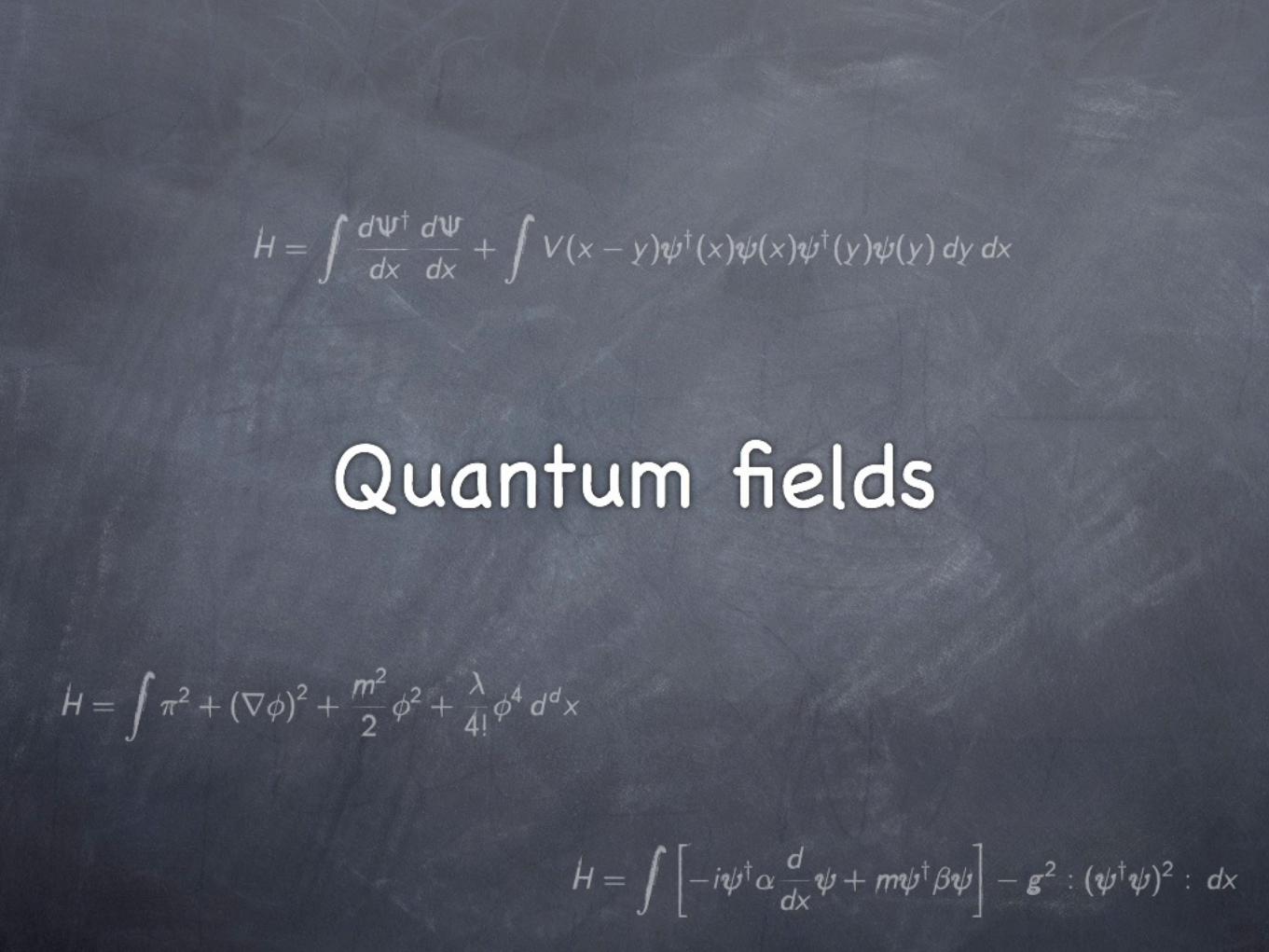
• Quantum fields

• The passage to the continuum

• Properties

• RG flow

• Area law

• Representations of ground states

• Variational method

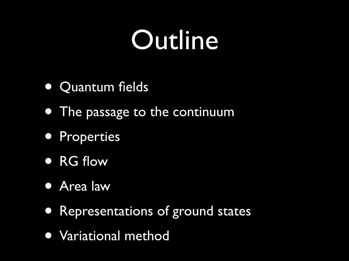
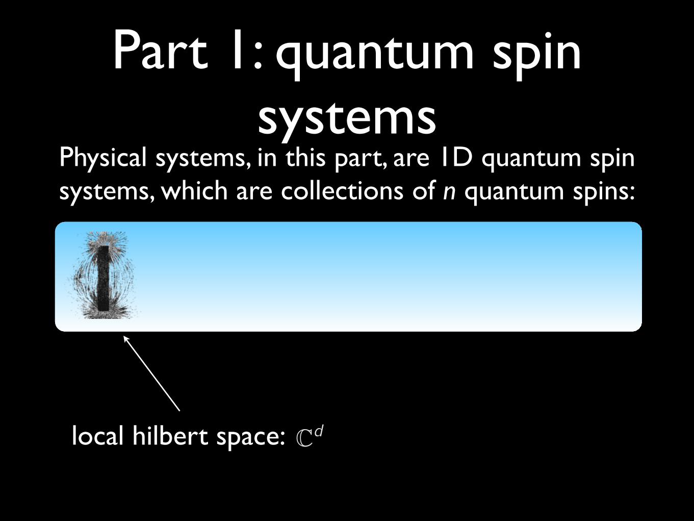
Part 1: quantum spin systems

Physical systems, in this part, are 1D quantum spin systems, which are collections of n quantum spins:

Part 1: quantum spin systems

Physical systems, in this part, are 1D quantum spin systems, which are collections of n quantum spins:

local hilbert space: Cd

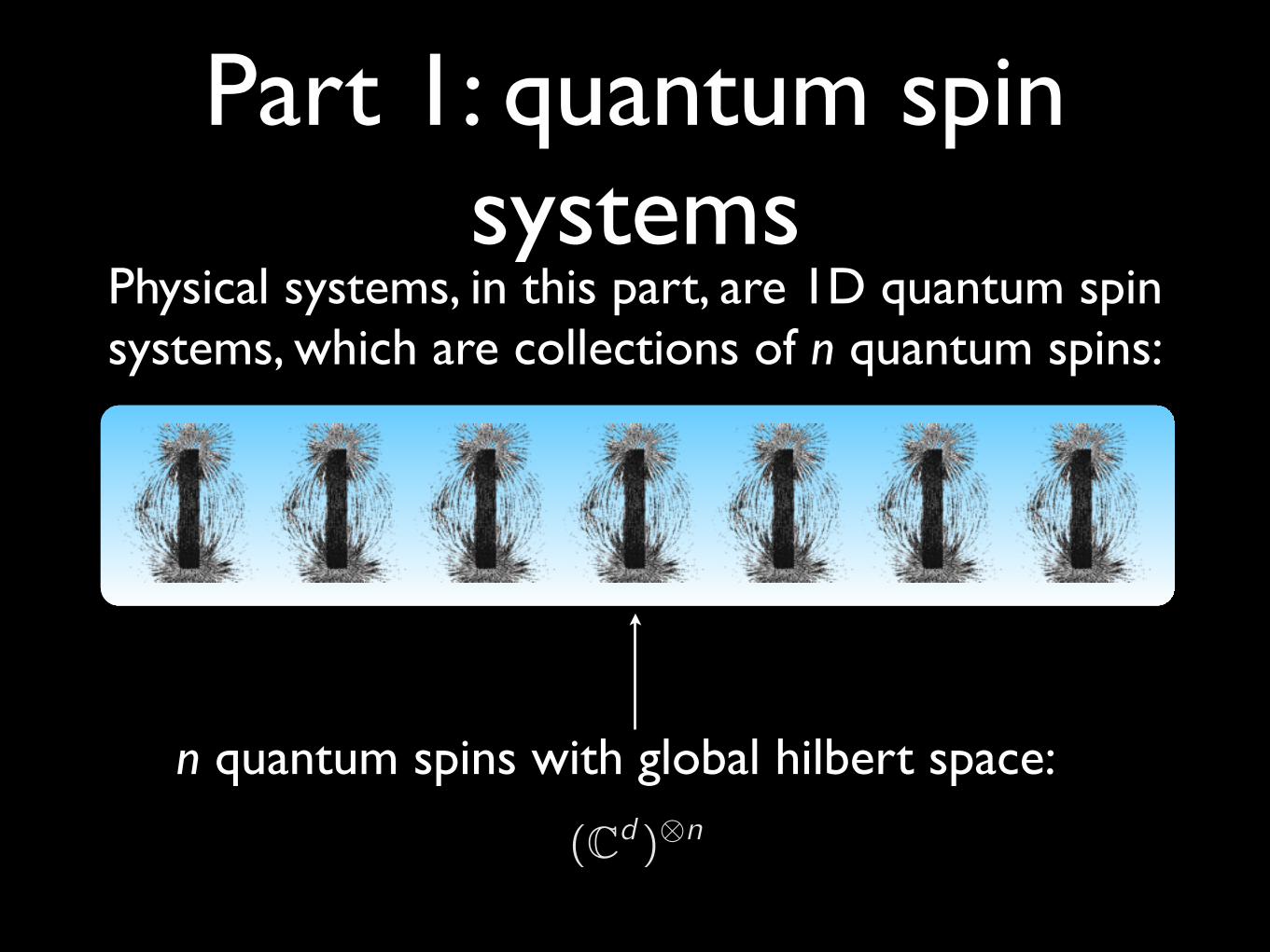
Part 1: quantum spin systems

Physical systems, in this part, are 1D quantum spin systems, which are collections of n quantum spins:

n quantum spins with global hilbert space:

(Cd)�n

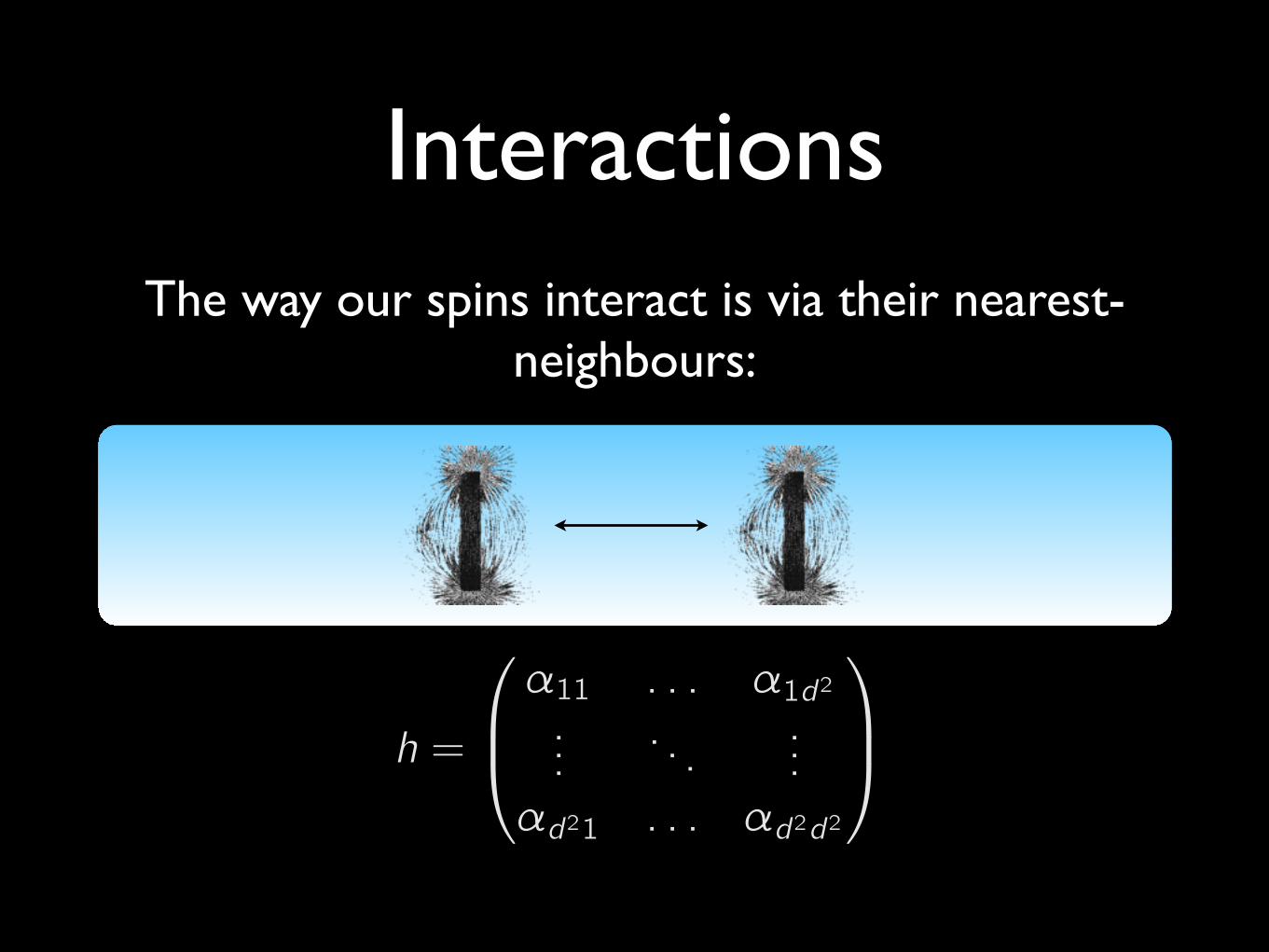
InteractionsThe way our spins interact is via their nearest-

neighbours:

h =

�

⇧⇤�11 . . . �1d2...

. . ....

�d21 . . . �d2d2

⇥

⌃⌅

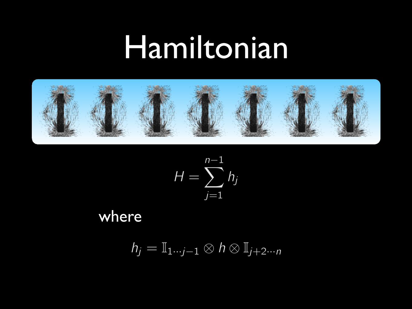
Hamiltonian

H =n�1�

j=1

hj

where

hj = I1···j�1 � h � Ij+2···n

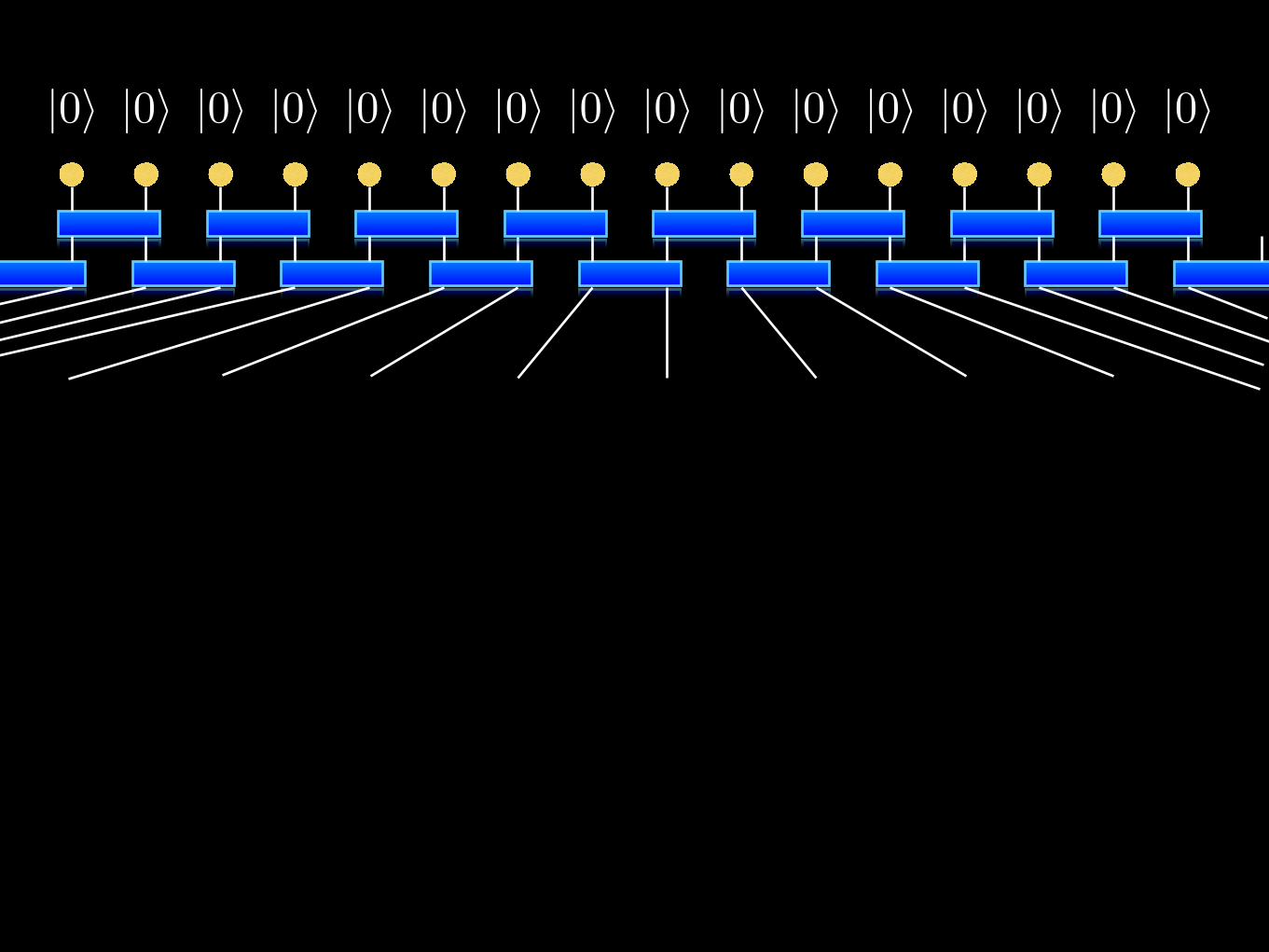
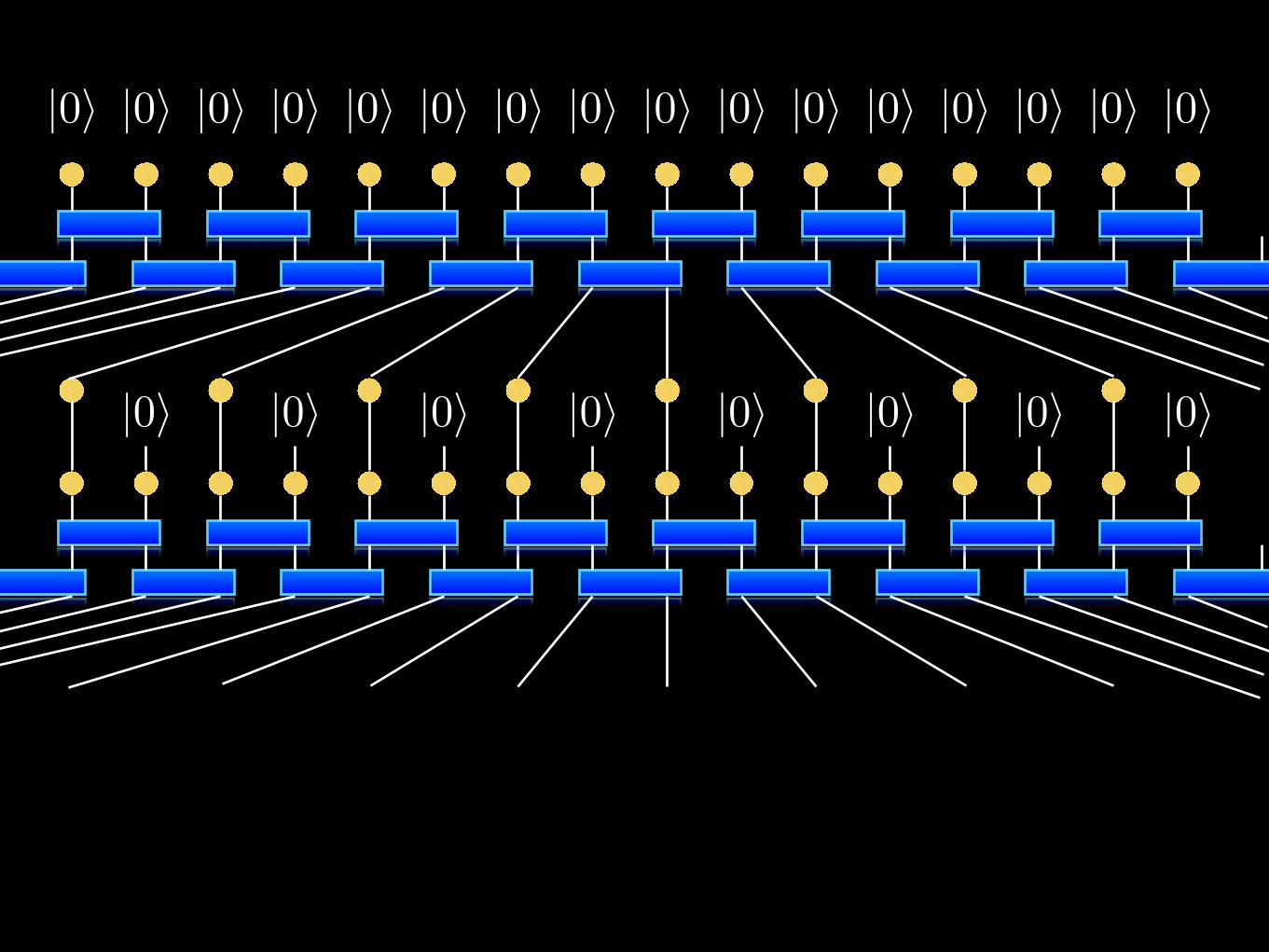
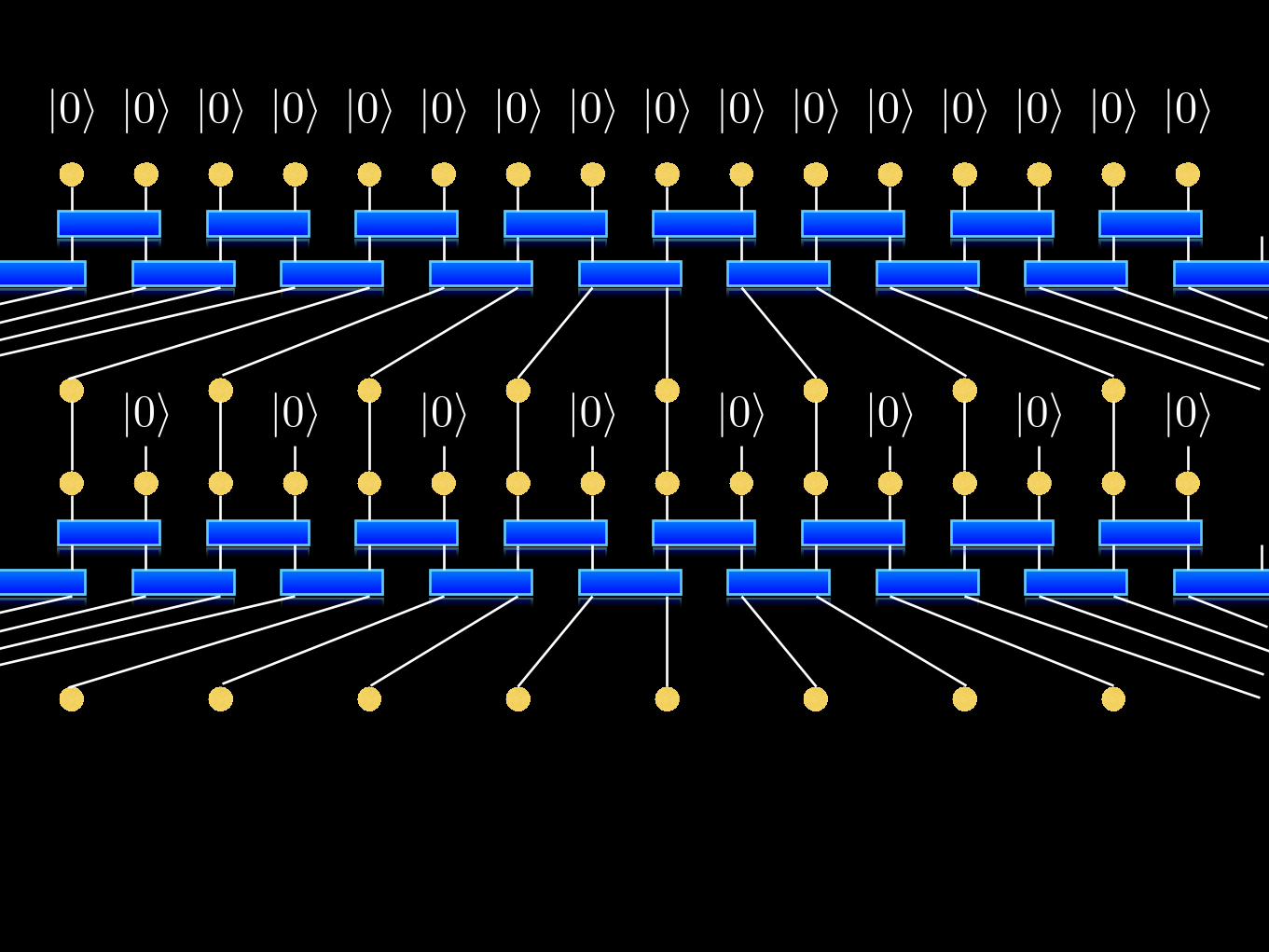
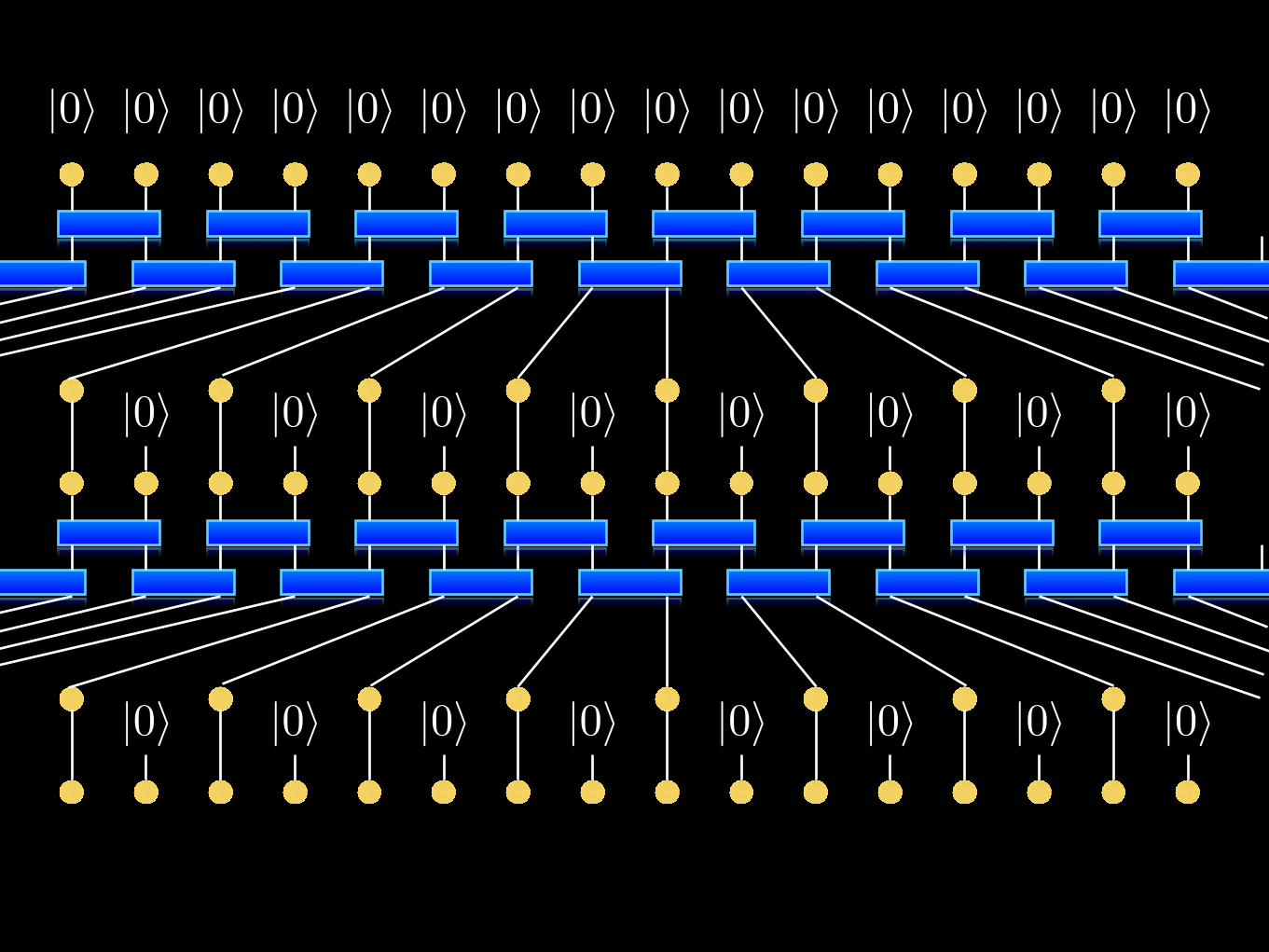
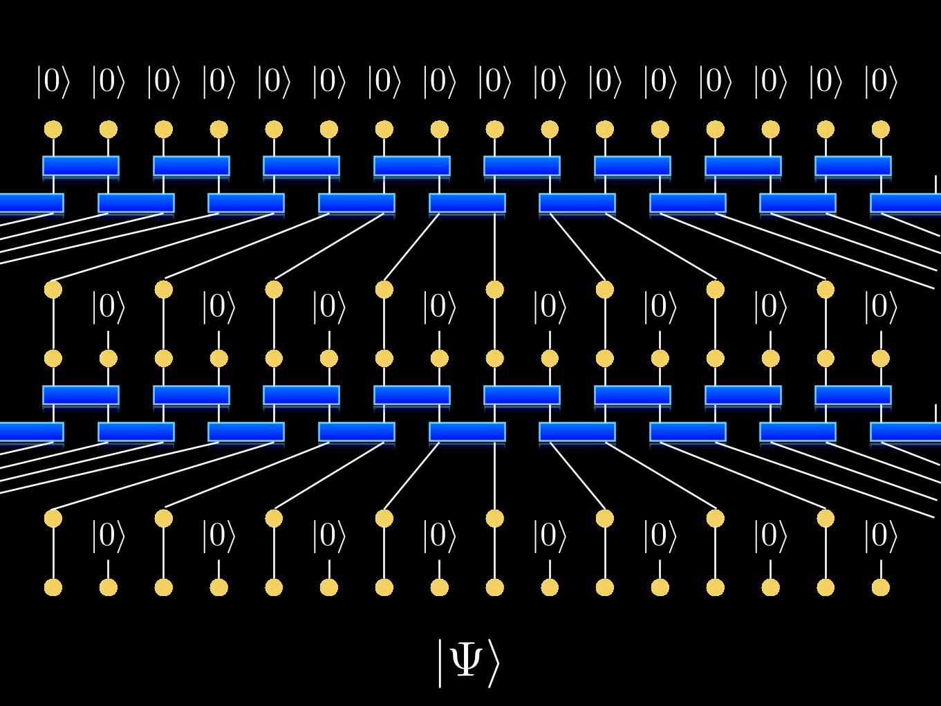
The multiscale entanglement

renormalisation ansatz

G. Vidal, Phys. Rev. Lett. 99, 220405 (2007)

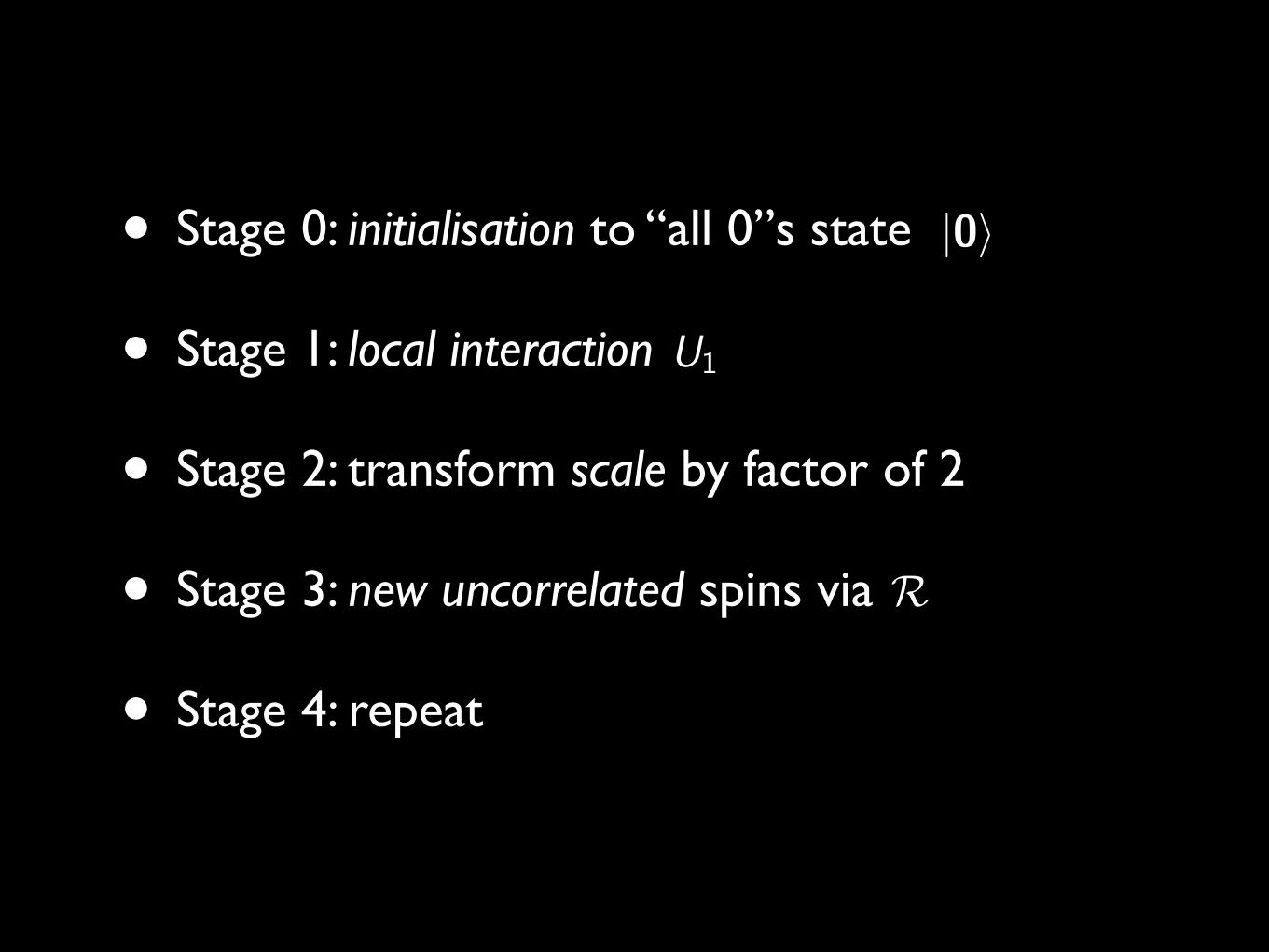
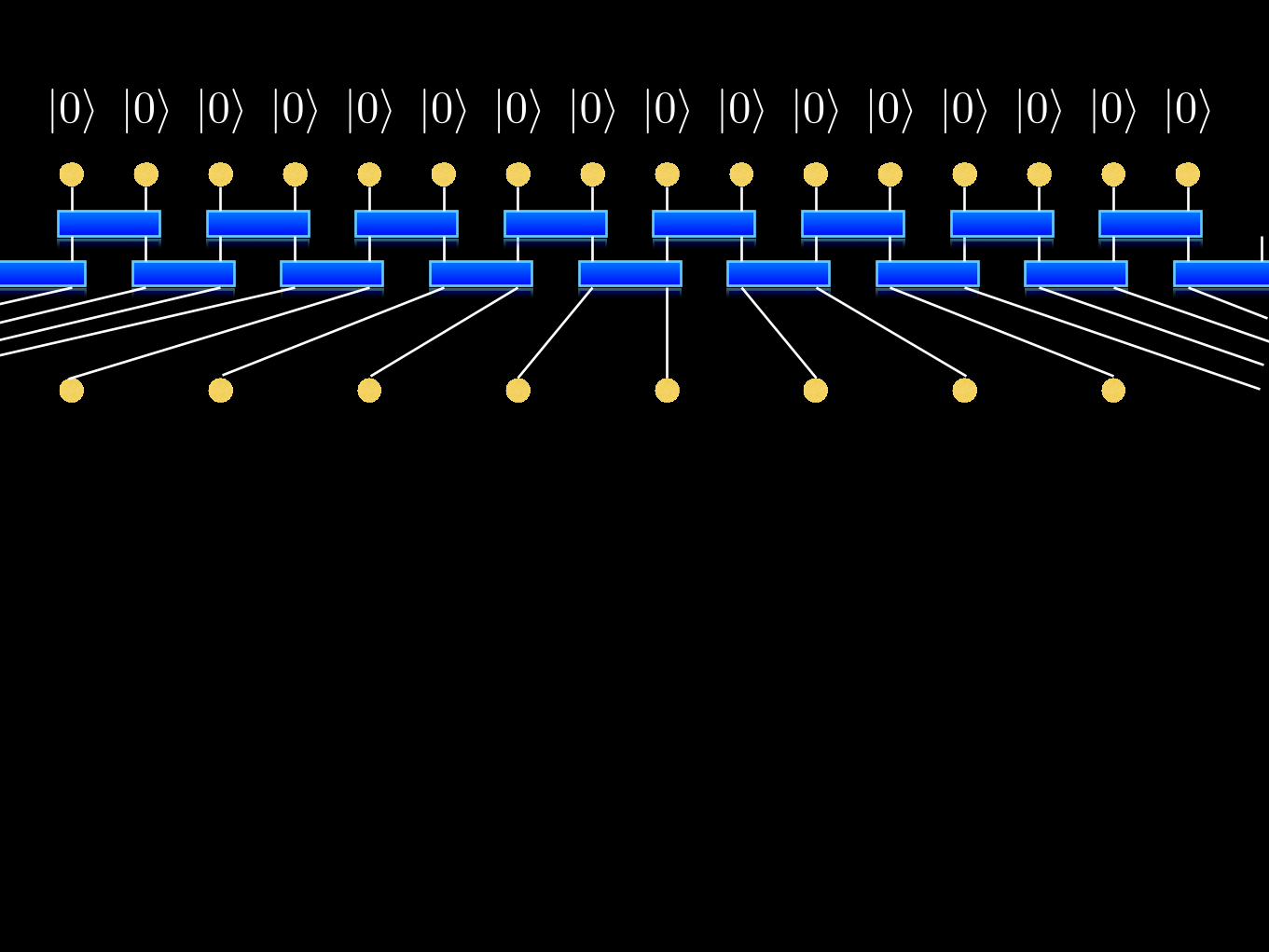
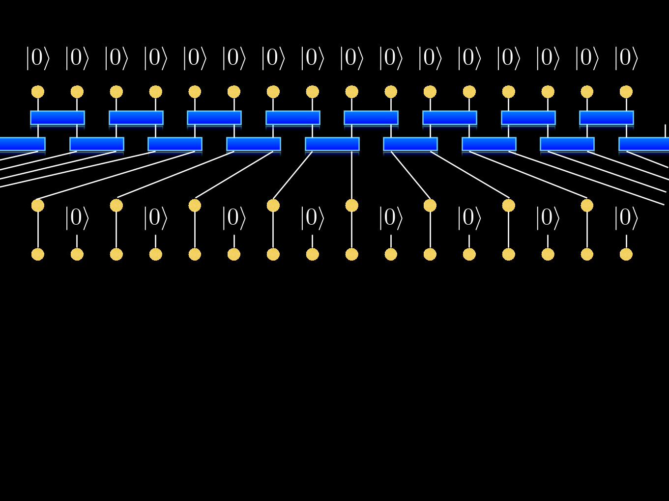
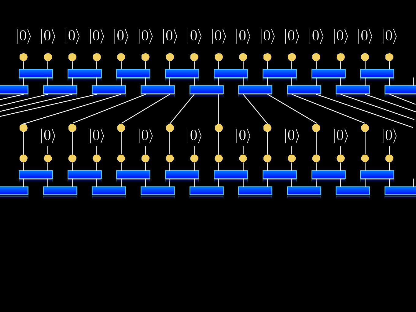
• Stage 0: initialisation to “all 0”s state

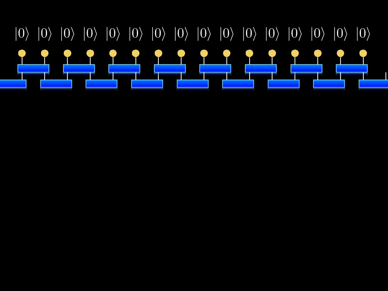
• Stage 1: local interaction

• Stage 2: transform scale by factor of 2

• Stage 3: new uncorrelated spins via

• Stage 4: repeat

|0�

U1

R

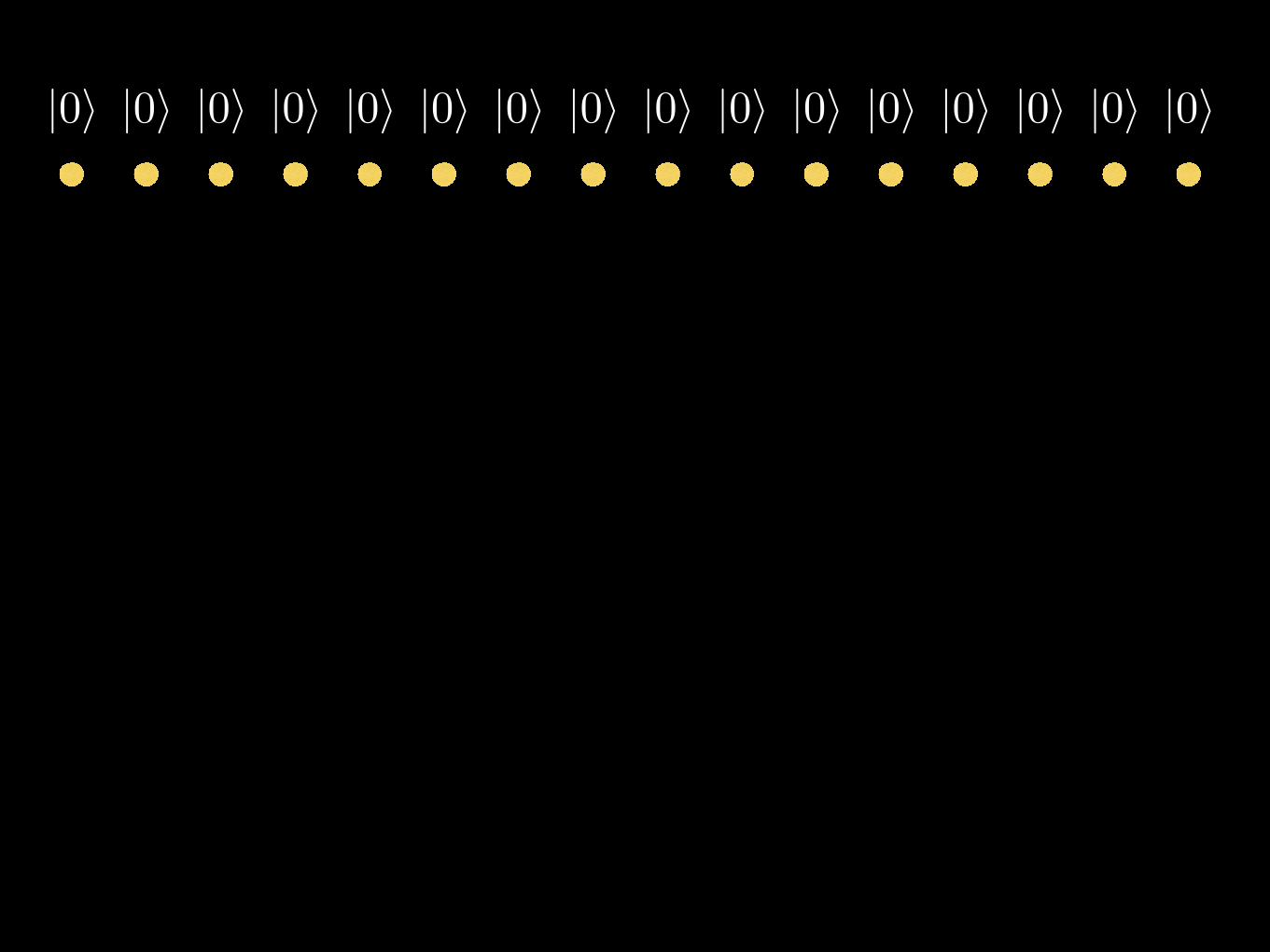
|0� |0� |0� |0� |0� |0� |0� |0� |0� |0� |0� |0� |0� |0� |0� |0�

|0� |0� |0� |0� |0� |0� |0� |0� |0� |0� |0� |0� |0� |0� |0� |0�

|0� |0� |0� |0� |0� |0� |0� |0� |0� |0� |0� |0� |0� |0� |0� |0�

|0� |0� |0� |0� |0� |0� |0� |0� |0� |0� |0� |0� |0� |0� |0� |0�

|0� |0� |0� |0� |0� |0� |0� |0� |0� |0� |0� |0� |0� |0� |0� |0�

|0� |0� |0� |0� |0� |0� |0� |0�

|0� |0� |0� |0� |0� |0� |0� |0� |0� |0� |0� |0� |0� |0� |0� |0�

|0� |0� |0� |0� |0� |0� |0� |0�

|0� |0� |0� |0� |0� |0� |0� |0� |0� |0� |0� |0� |0� |0� |0� |0�

|0� |0� |0� |0� |0� |0� |0� |0�

|0� |0� |0� |0� |0� |0� |0� |0� |0� |0� |0� |0� |0� |0� |0� |0�

|0� |0� |0� |0� |0� |0� |0� |0�

|0� |0� |0� |0� |0� |0� |0� |0� |0� |0� |0� |0� |0� |0� |0� |0�

|0� |0� |0� |0� |0� |0� |0� |0�

|0� |0� |0� |0� |0� |0� |0� |0�

|0� |0� |0� |0� |0� |0� |0� |0� |0� |0� |0� |0� |0� |0� |0� |0�

|0� |0� |0� |0� |0� |0� |0� |0�

|0� |0� |0� |0� |0� |0� |0� |0�

| �

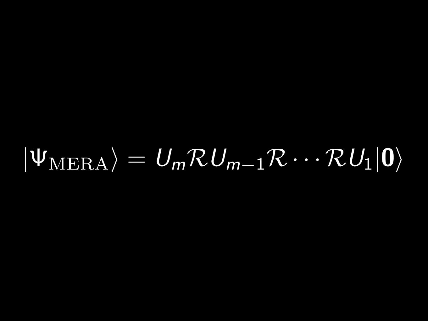
|�MERA� = UmRUm�1R· · ·RU1|0�

MERA = dilation + local interaction

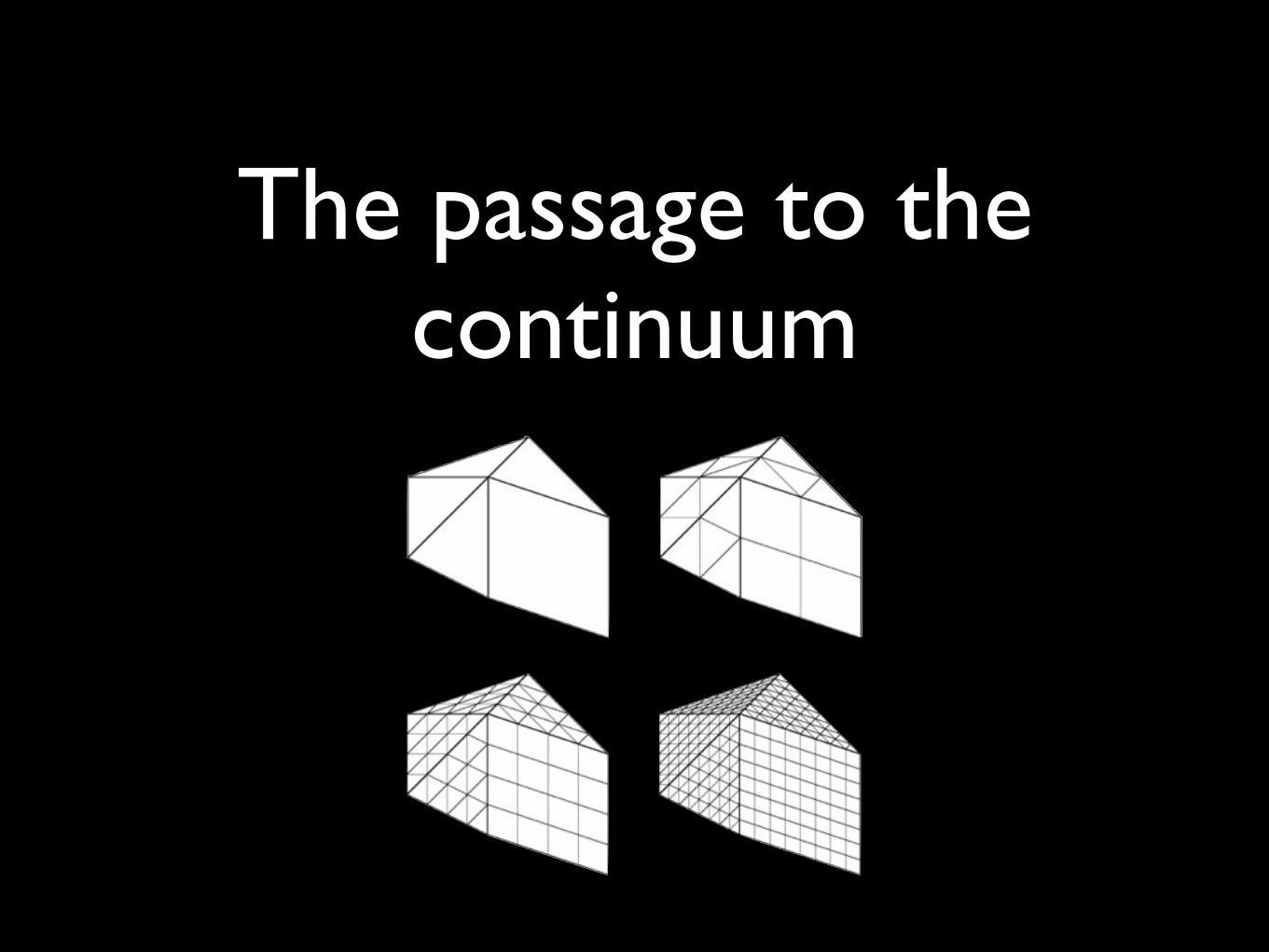
The passage to the continuum

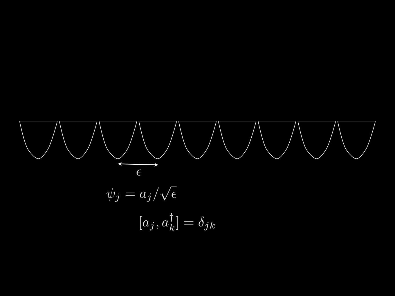
⇥j = aj/p�

[aj , a†k] = �jk

✏

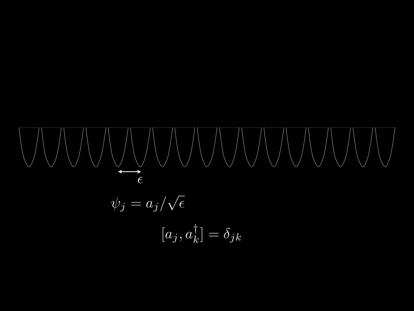
⇥j = aj/p�

[aj , a†k] = �jk

✏

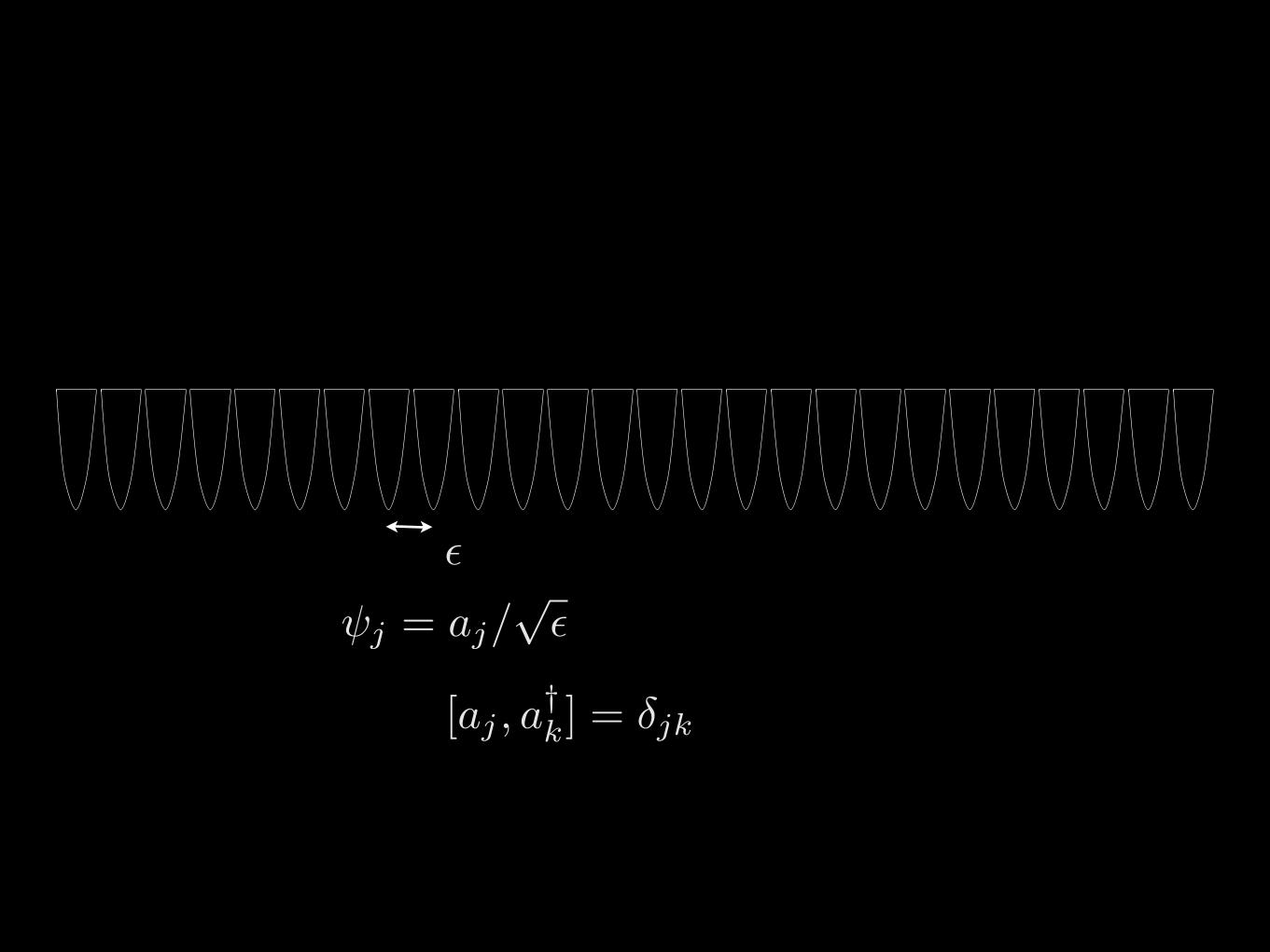
⇥j = aj/p�

[aj , a†k] = �jk

✏

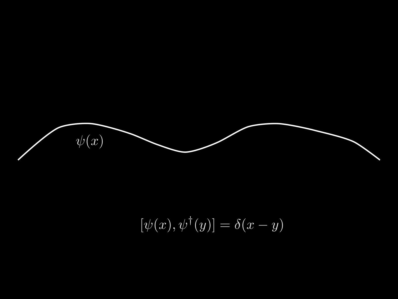
[⇥(x),⇥†(y)] = �(x� y)

�(x)

cMERA

Idea: make everything infinitesimal

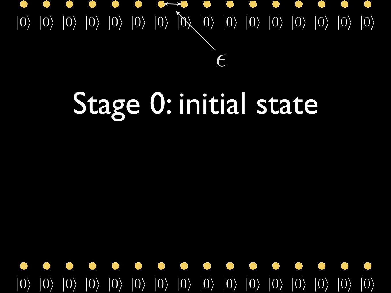
Stage 0: initial state

|0� |0� |0� |0� |0� |0� |0� |0� |0� |0� |0� |0� |0� |0� |0� |0�

|0� |0� |0� |0� |0� |0� |0� |0� |0� |0� |0� |0� |0� |0� |0� |0�

✏

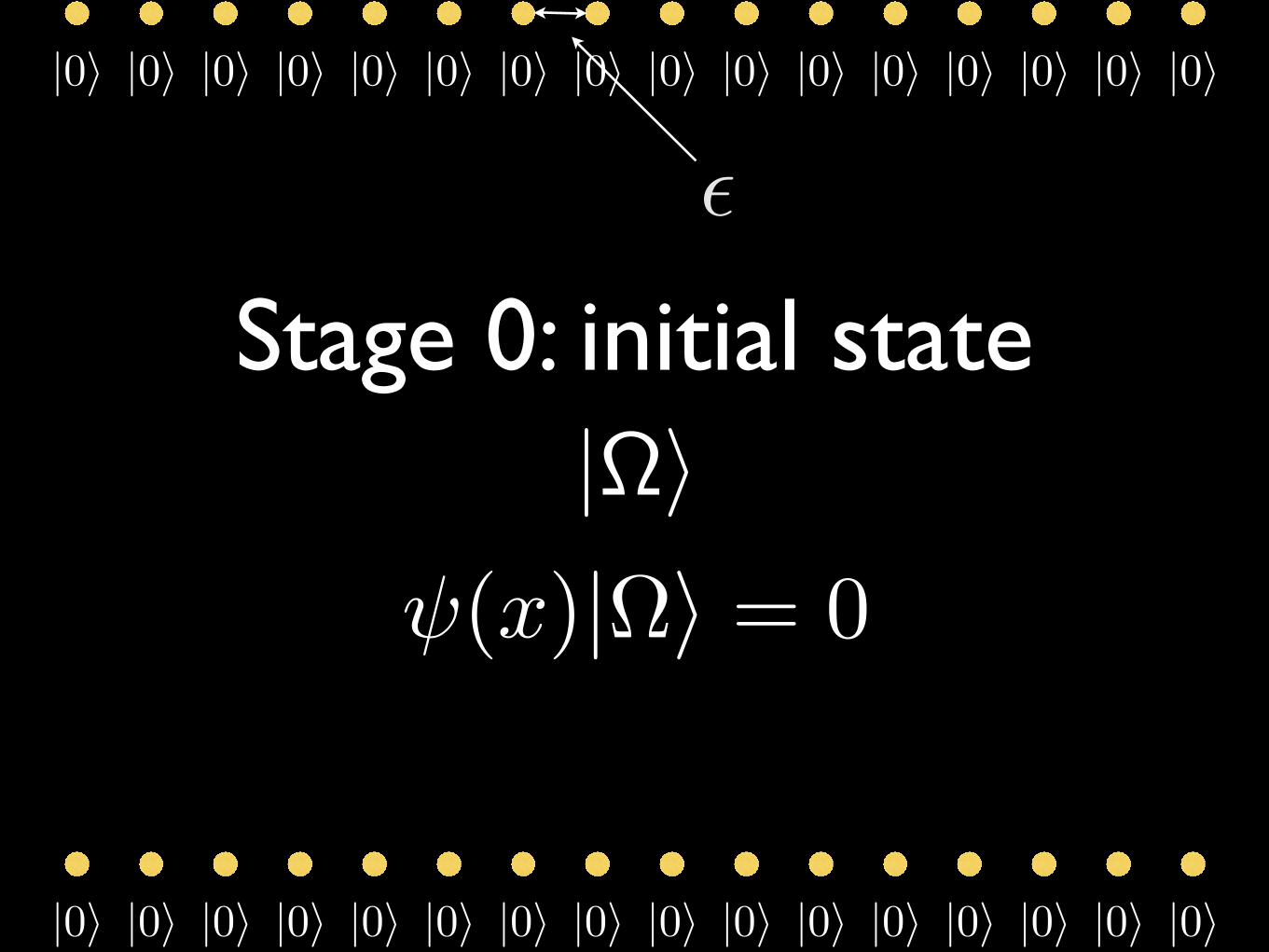
Stage 0: initial state

|0� |0� |0� |0� |0� |0� |0� |0� |0� |0� |0� |0� |0� |0� |0� |0�

|0� |0� |0� |0� |0� |0� |0� |0� |0� |0� |0� |0� |0� |0� |0� |0�

✏

|⌦��(x)|�� = 0

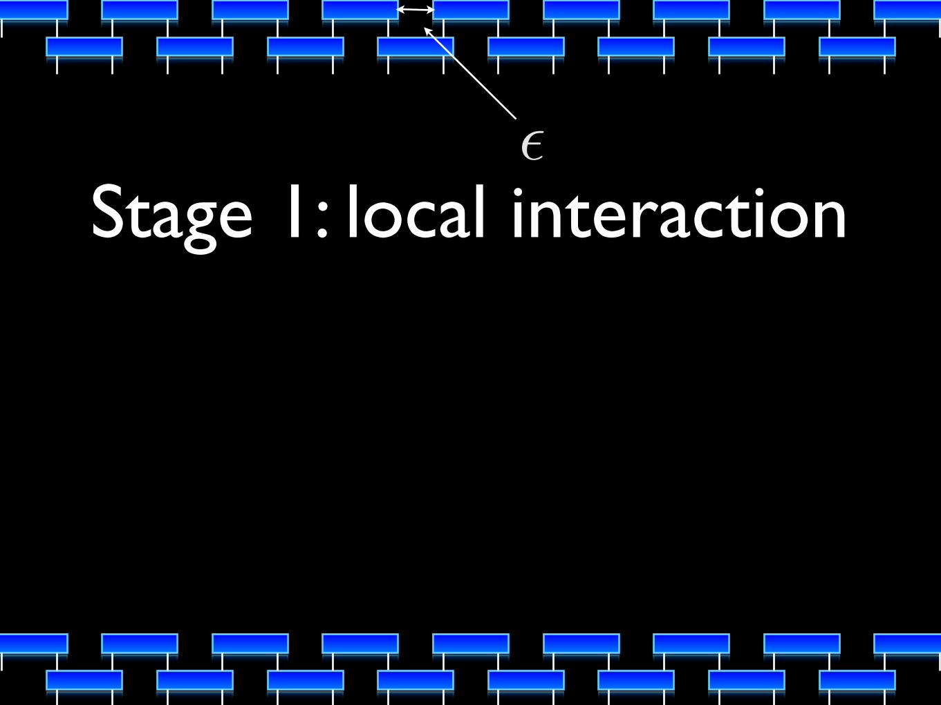
Stage 1: local interaction✏

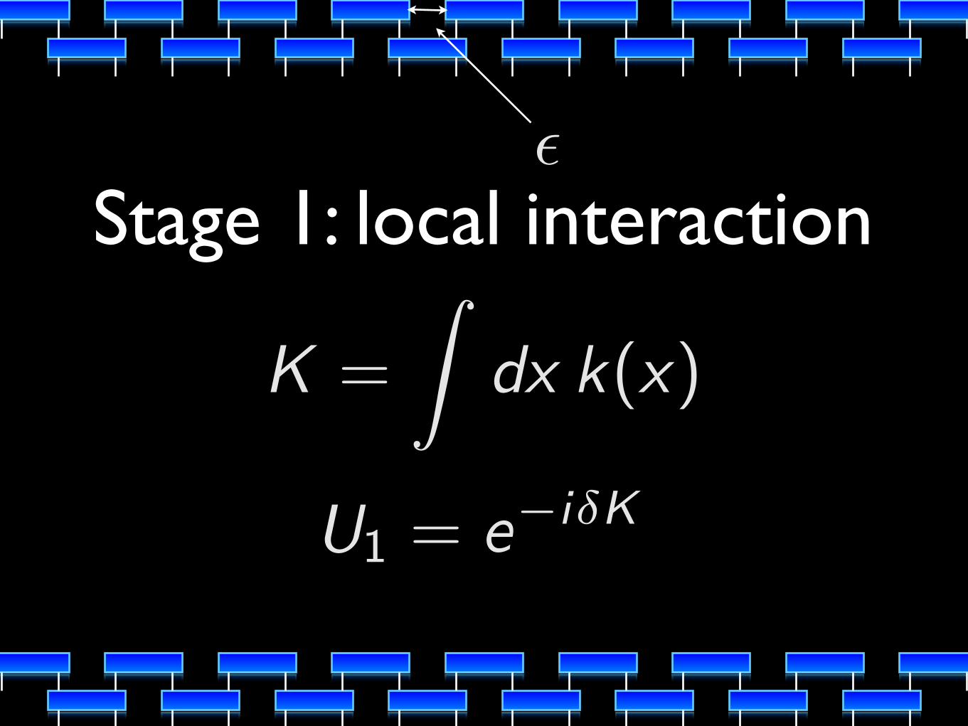
Stage 1: local interaction✏

K =

Zdx k(x)

U1 = e�i�K

Stage 2: scale transform

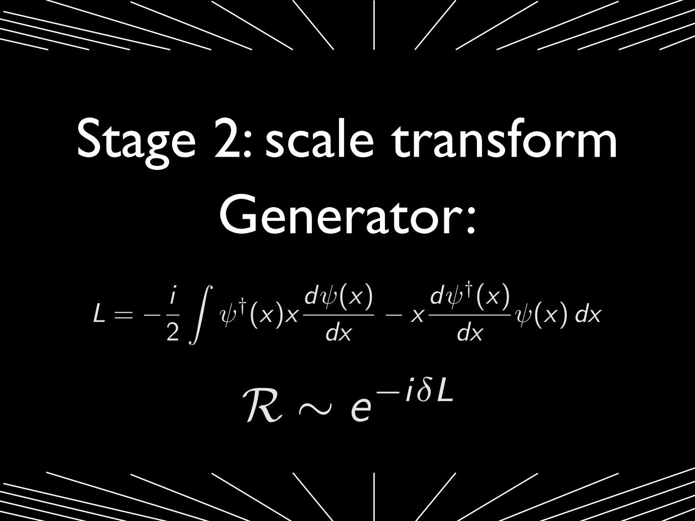
Stage 2: scale transformGenerator:

L = � i

2

Z †(x)x

d (x)

dx

� x

d †(x)

dx

(x) dx

R � e�i�L

Stage 3: new degrees of freedom?

Answer: impose UV cutoff on K

Why?

Why?

✏ ⇠ 1

�

Gives lengthscale

(Bad) example:

K =

Z †2(x) + 2(x)dx

uncorrelated degrees of freedom

come from high mtm viaR � e�i�L

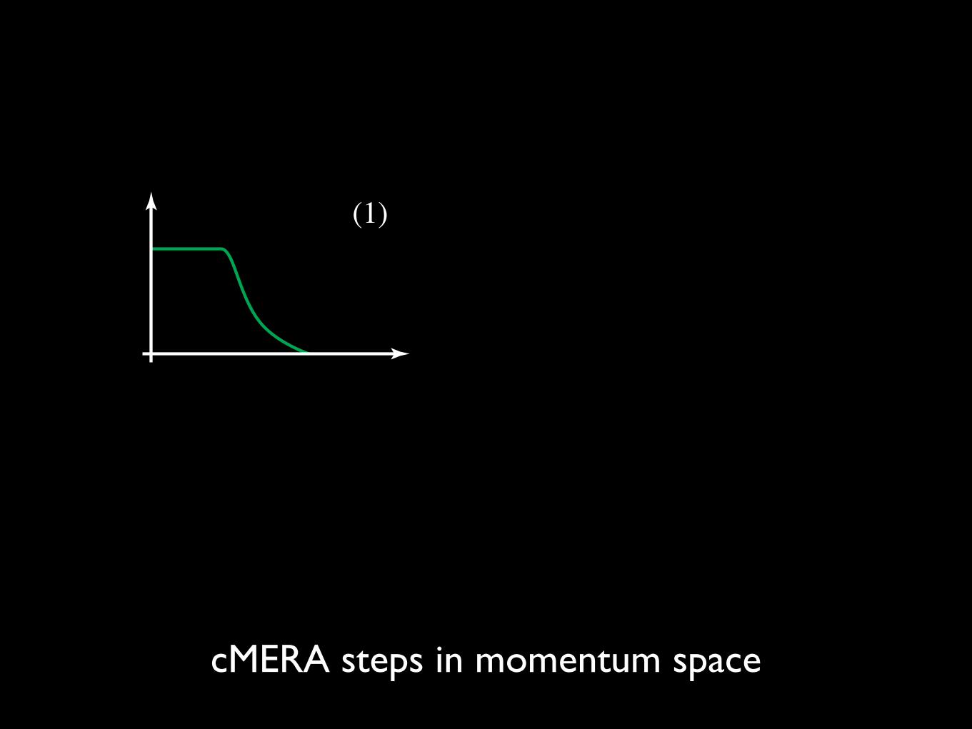
cMERA steps in momentum space

(1) (2)

(3) (4)

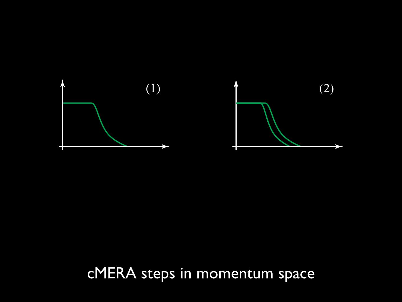
cMERA steps in momentum space

(1) (2)

(3) (4)

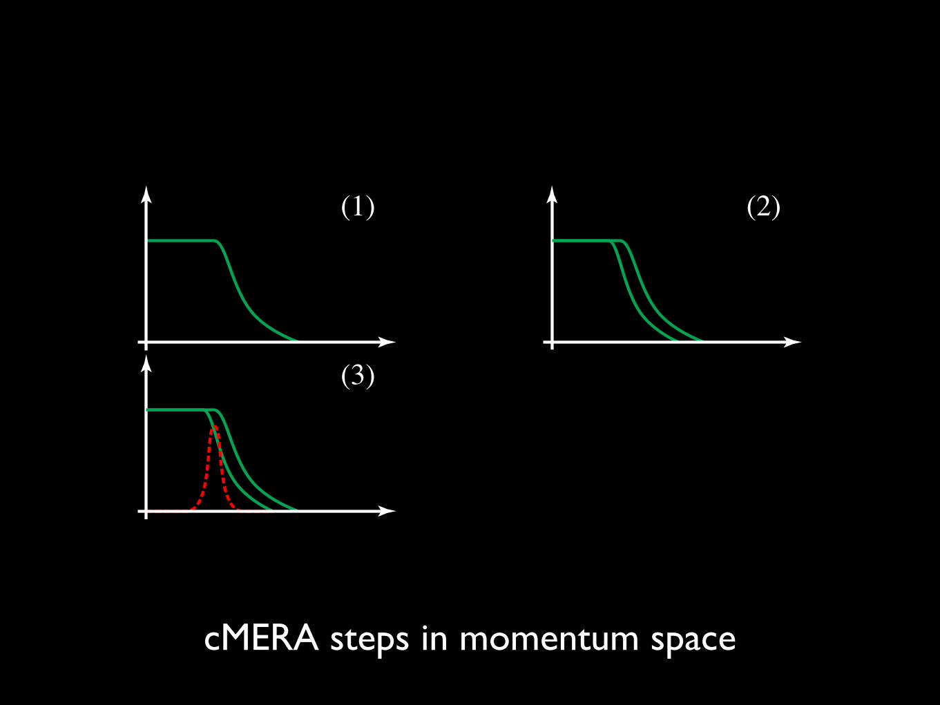
cMERA steps in momentum space

(1) (2)

(3) (4)

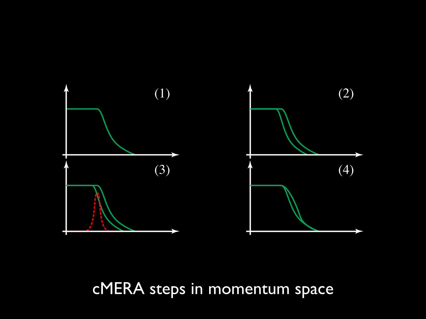
cMERA steps in momentum space

(1) (2)

(3) (4)

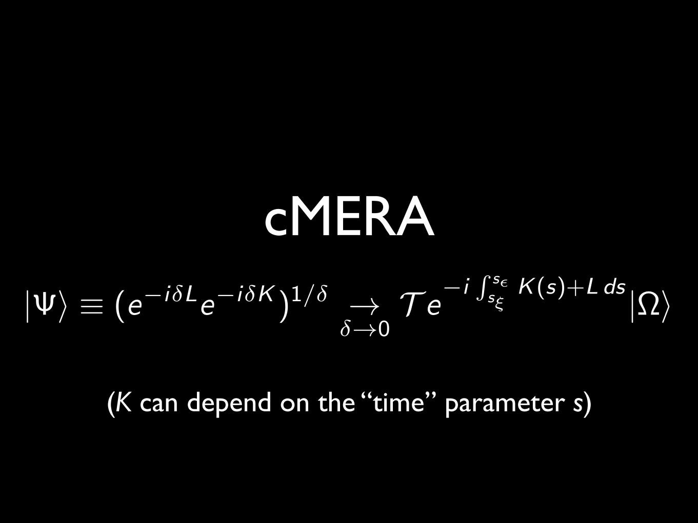
cMERA|�⇤ � (e�i�Le�i�K )1/� ⇥

�!0T e

�iR s✏s⇠

K(s)+L ds |⇥⇤

(K can depend on the “time” parameter s)

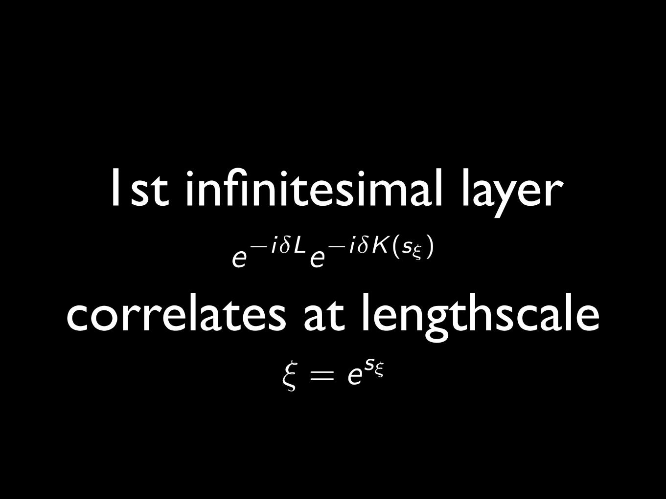
1st infinitesimal layer

correlates at lengthscalee�i�Le�i�K(s⇠)

⇠ = es⇠

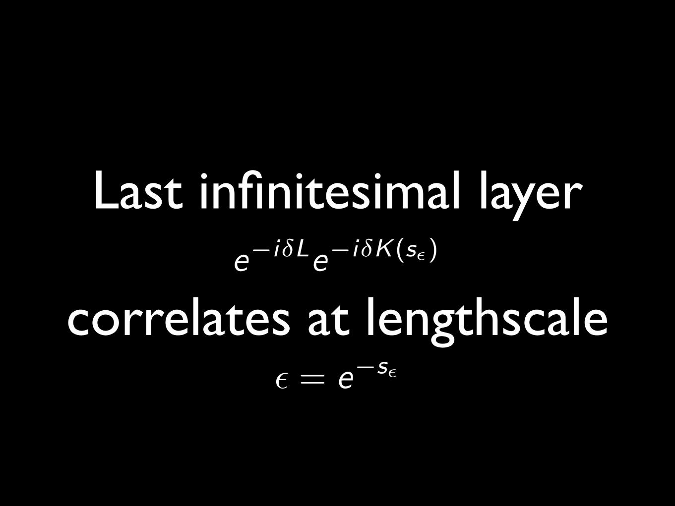
Last infinitesimal layer

correlates at lengthscalee�i�Le�i�K(s✏)

✏ = e�s✏

cMERA have fluctuations from to ⇠ ✏ ⇠ ⇠

cMERA vs MERA:

cMERA vs MERA:UV cutoff

MERA = lattice cutoffcMERA = smooth cutoff

RG flow

cMERA (Schr. pic.): variational class

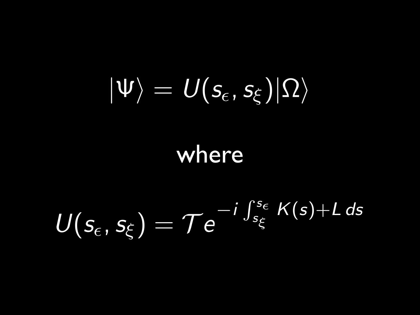
| i = U(s✏, s⇠)|⌦i

U(s✏, s⇠) = T e�i

R s✏s⇠

K(s)+L ds

where

cMERA (Heis. pic.): renormalization

group flow

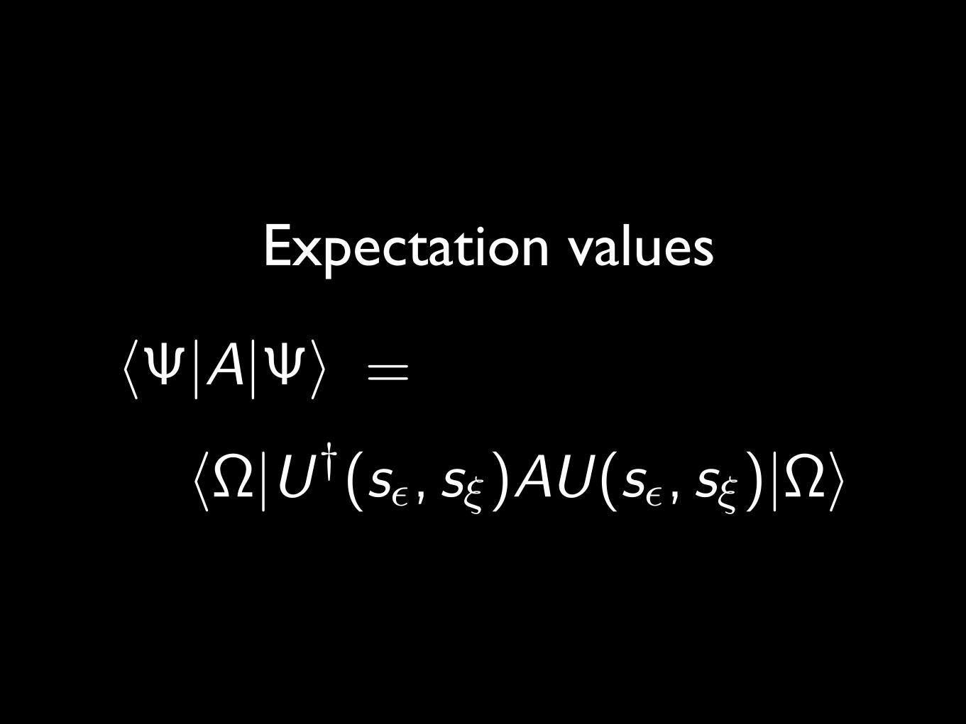
Expectation values

Expectation values

h |A| i

Expectation values

h |A| i =

Expectation values

h |A| i

h⌦|U†(s✏, s⇠)AU(s✏, s⇠)|⌦i

=

AR(s) ⌘ U†(s✏, s)AU(s✏, s)

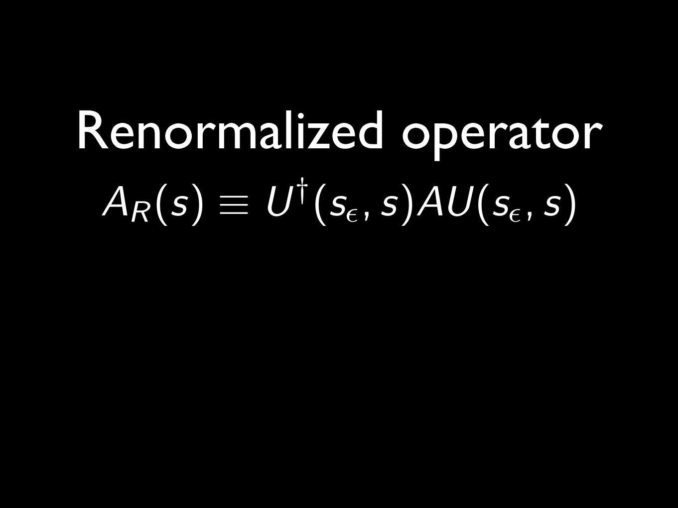
Renormalized operator

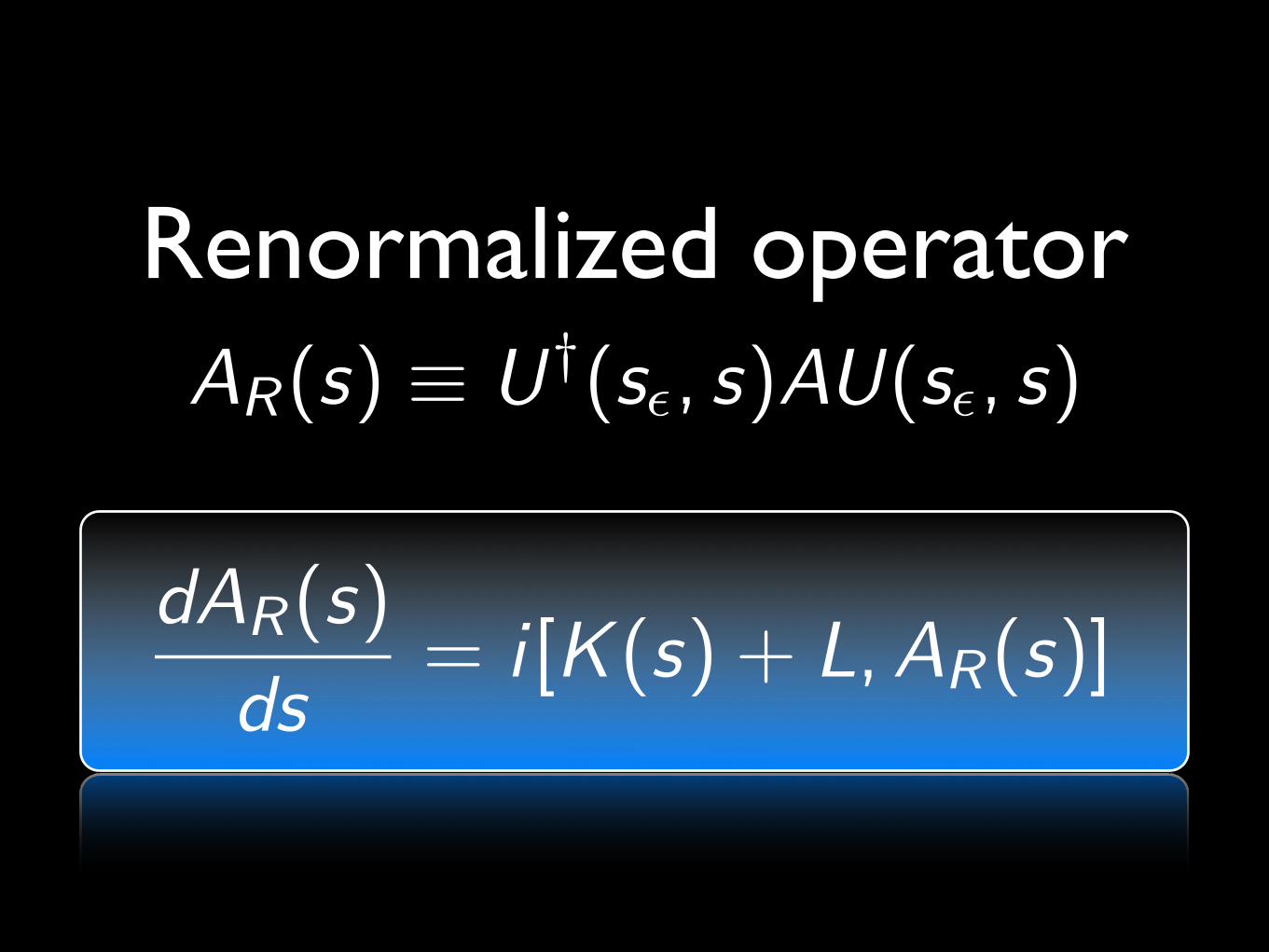
AR(s) ⌘ U†(s✏, s)AU(s✏, s)

Renormalized operator

dAR(s)

ds= i [K (s) + L,AR(s)]

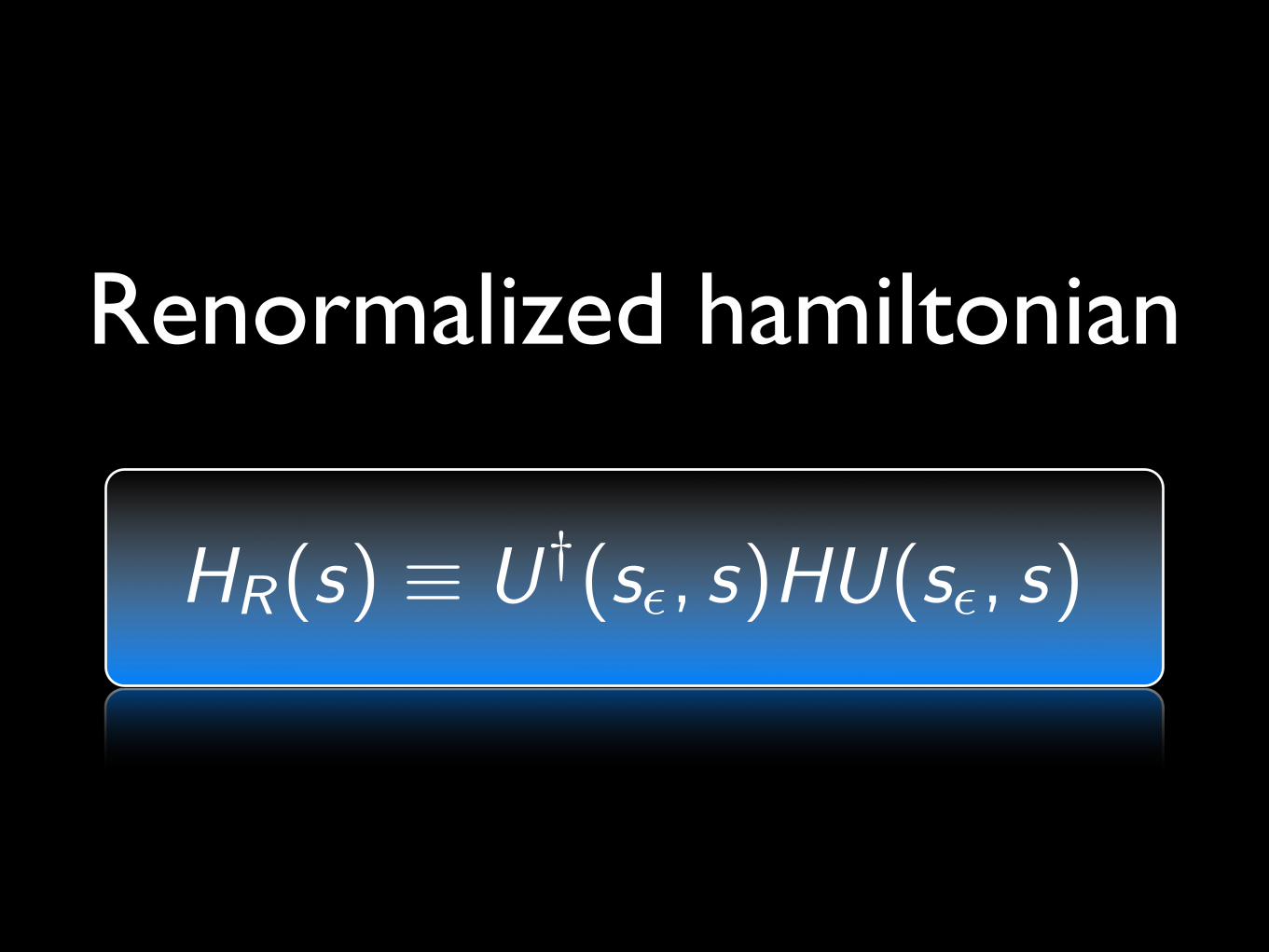
Renormalized hamiltonian

HR(s) ⌘ U†(s✏, s)HU(s✏, s)

RG Flow on theories

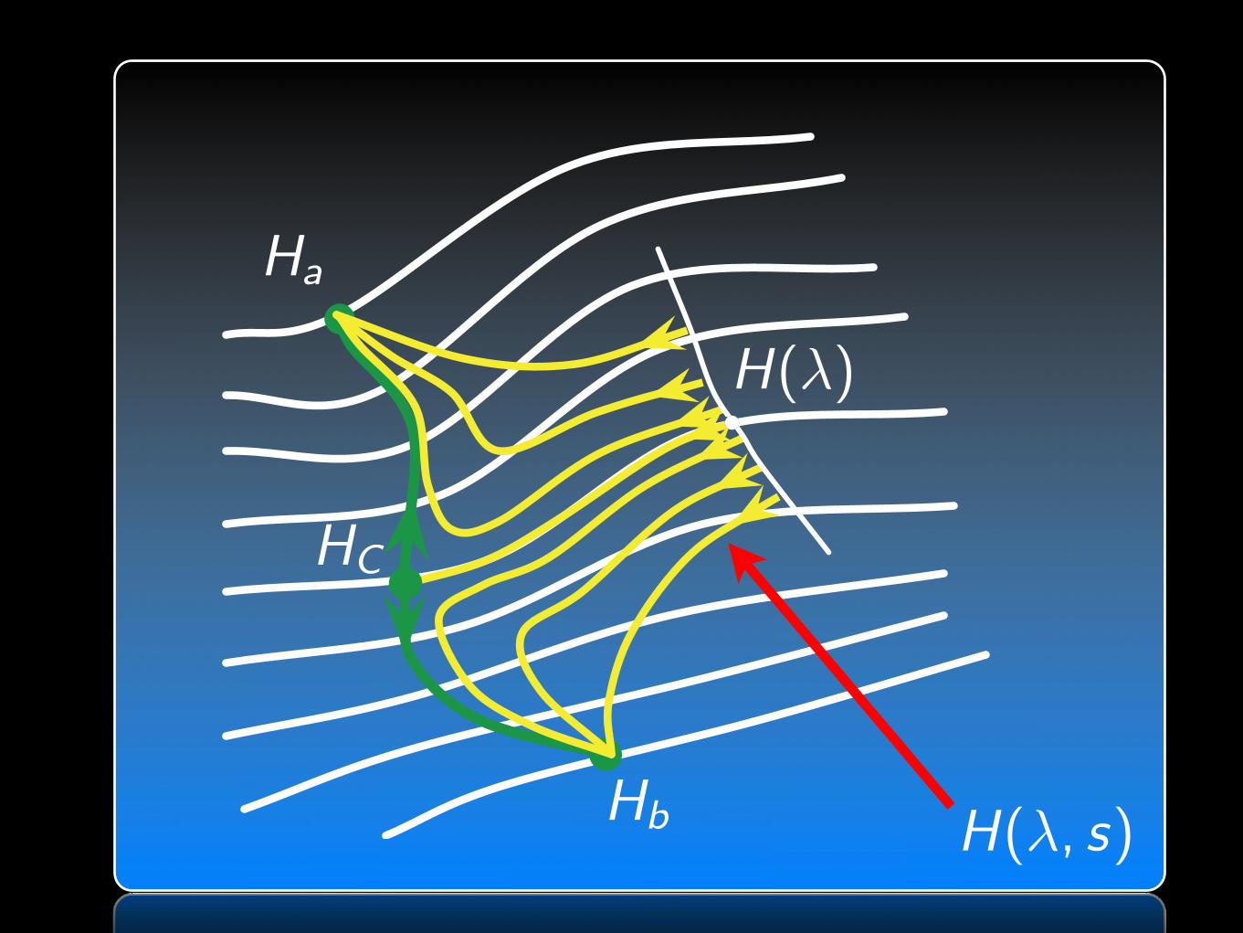
HC

Ha

Hb

H(�)

H(�, s)

Entropy/area laws

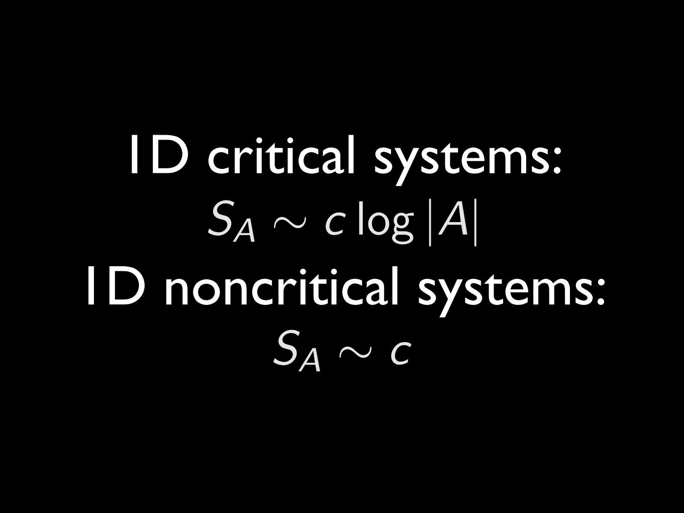
1D critical systems:SA � c log |A|

SA ⇠ c1D noncritical systems:

Standard MERA can giveSA � c log |A|

cMERA?

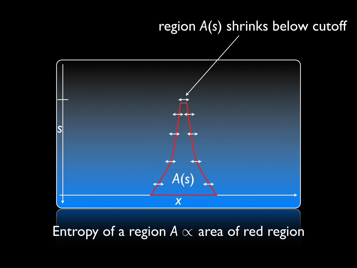
Entropy of a region A area of red region

x

s

A(s)

region A(s) shrinks below cutoff

/

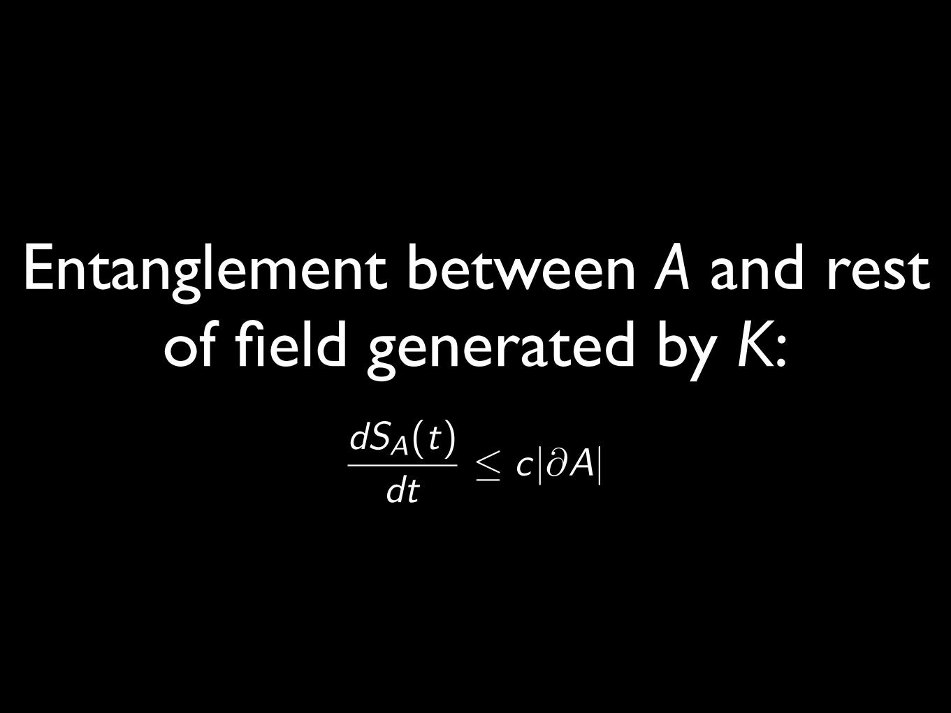
Entanglement between A and rest of field generated by K:

dSA(t)

dt� c |@A|

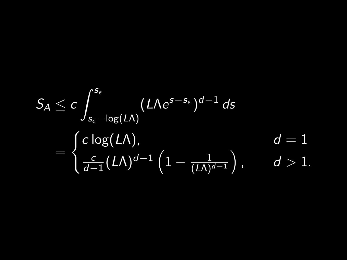
SA c

Z s✏

s✏�log(L�)(L�es�s✏)d�1 ds

=

(c log(L�), d = 1c

d�1 (L�)d�1

⇣1� 1

(L�)d�1

⌘, d > 1.

Ground states

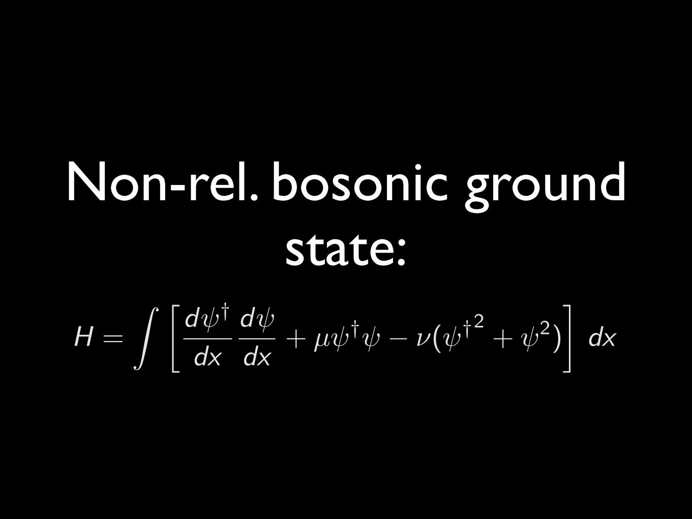
Non-rel. bosonic ground state:

H =

Z d⇥†

dx

d⇥

dx+ µ⇥†⇥ � �(⇥†2 + ⇥2)

�dx

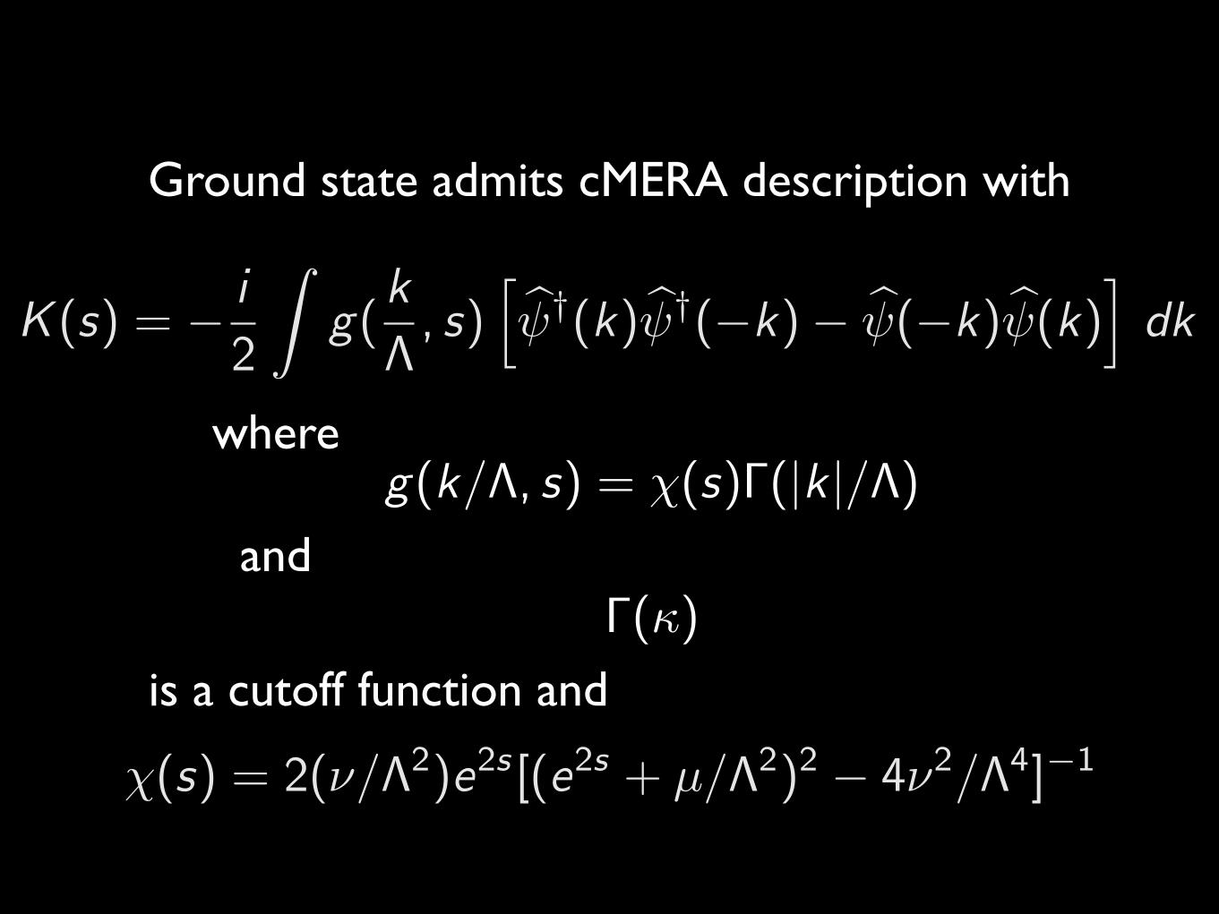
K (s) = � i

2

Zg(

k

�, s)

hb †(k) b †(�k)� b (�k) b (k)

idk

g(k/⇥, s) = �(s)�(|k |/⇥)

�()

where

and

is a cutoff function and

Ground state admits cMERA description with

⇥(s) = 2(�/�2)e2s [(e2s + µ/�2)2 � 4�2/�4]�1

Another path to continuum: causal structure

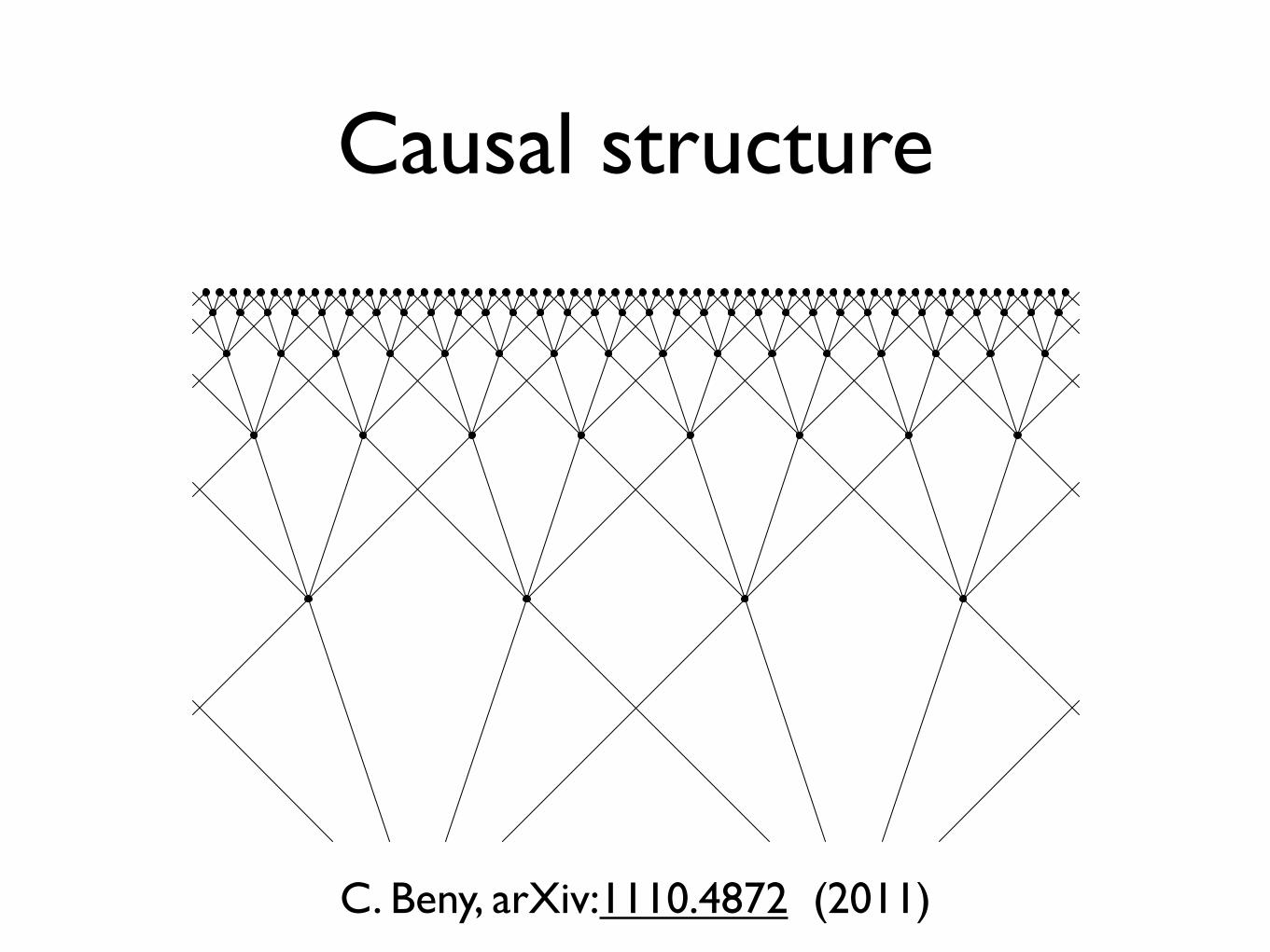
Causal structure

C. Beny, arXiv:1110.4872 (2011)

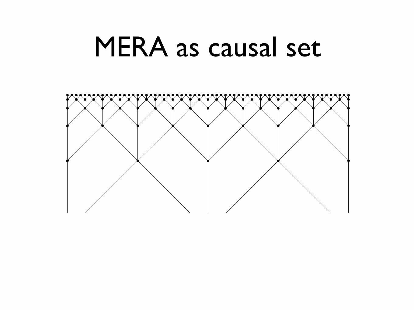
MERA as causal set

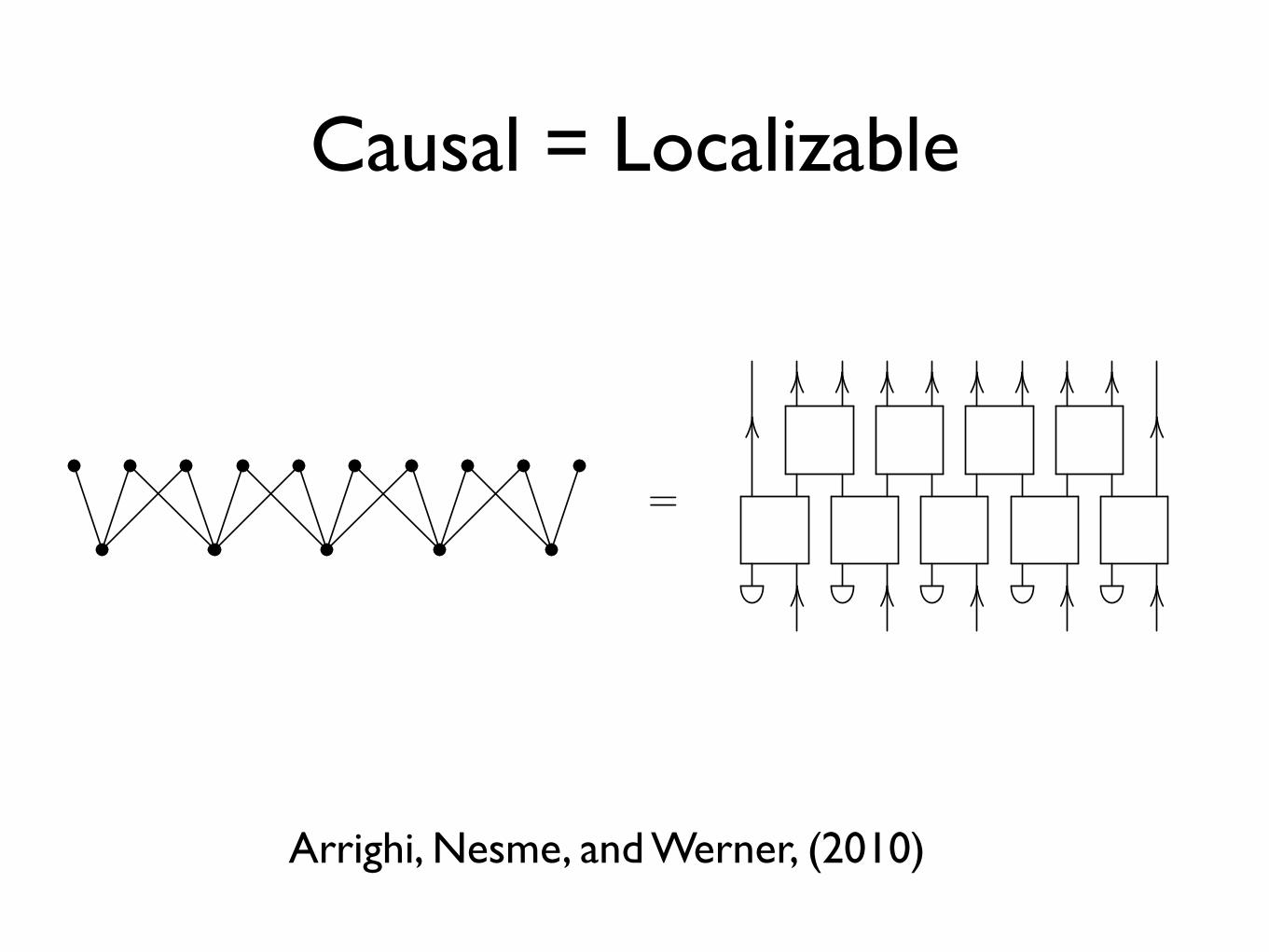
Causal = Localizable

=

OO OO OO OO OO

OOOO OO OO OOOO OO OO OO

OO

Arrighi, Nesme, and Werner, (2010)

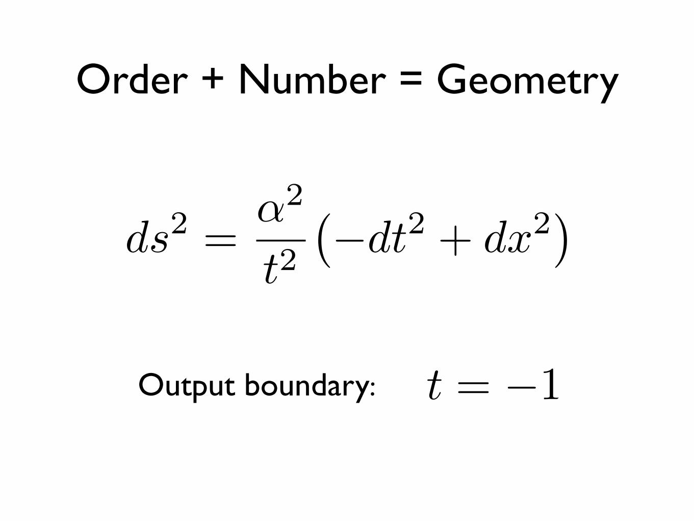
Order + Number = Geometry

ds

2 =↵

2

t

2

��dt

2 + dx

2�

Output boundary: t = �1

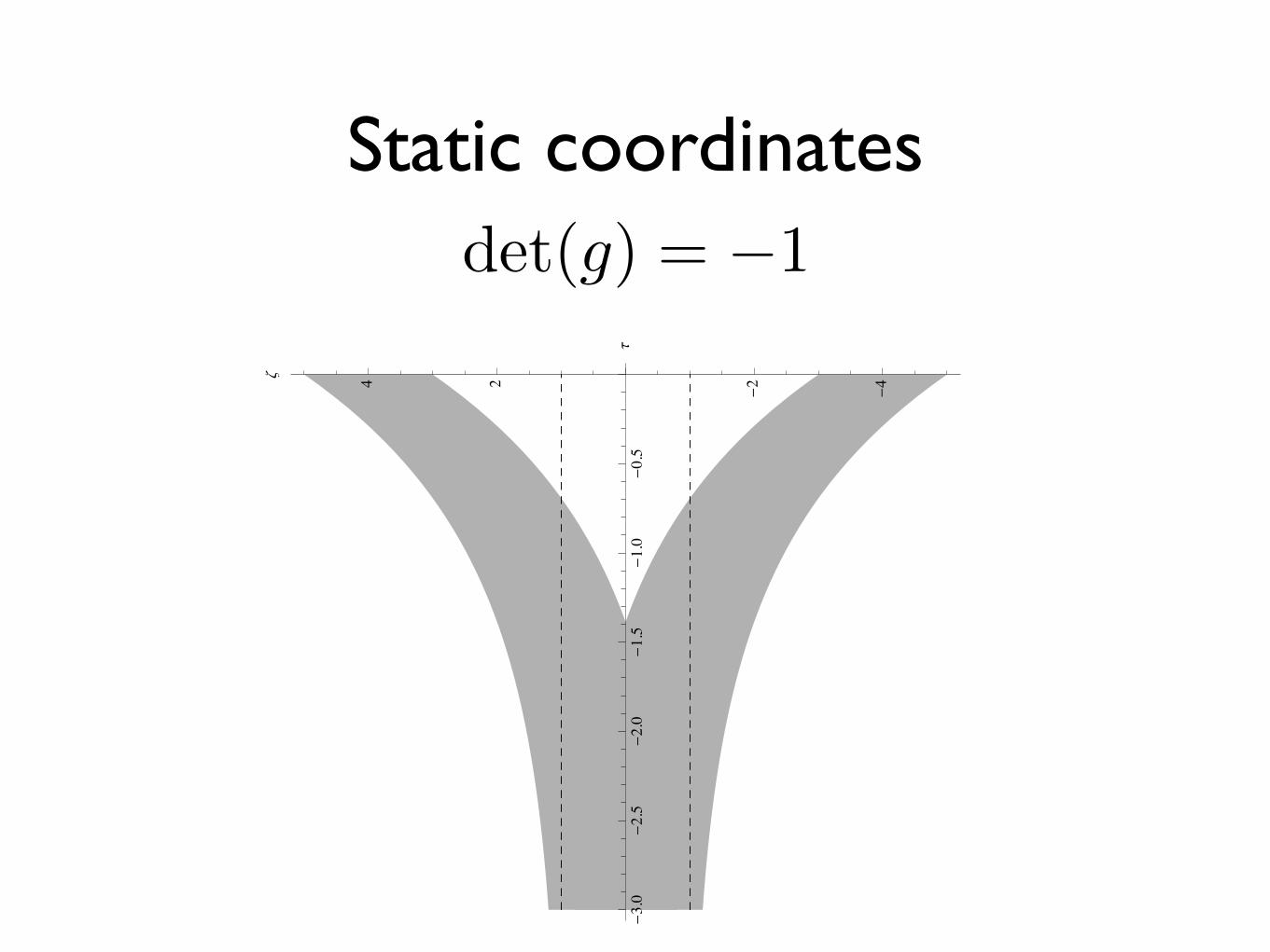
Static coordinatesdet(g) = �1

!3.0

!2.5

!2.0

!1.5

!1.0

!0.5

"

!4

!224#

cMERA

cMERA = Dilation + UV cutoff

cMERA = Dilation + UV cutoff

preserve symmetries

cMERA = Dilation + UV cutoff

preserve symmetries

capture ground states