Embed Size (px)
Citation preview

Term Structure of Uncertainty:
New Evidence from Survey
Expectations∗
Carola Binder† Tucker S. McElroy‡ Xuguang S. Sheng§
Abstract
We construct measures of individual forecasters’ subjective uncertainty at horizons ranging
from one to five years, incorporating a rich information set from the European Central Bank’s
Survey of Professional Forecasters. Our measures have two key advantages over traditional
measures: (i) they reflect the subjective perceptions of market participants; (ii) they are ex ante
measures that do not require the knowledge of realized outcomes. We find that the uncertainty
curve is much more linear than the disagreement curve — uncertainty at the one-year and
two-year horizons can almost perfectly predict uncertainty at the five-year horizon, but not so
for disagreement. We develop a learning model that captures the two channels through which
large shocks affect the term structure of uncertainty: wake-up effect — the visibly large shocks
induce immediate and synchronized updating of information for economic agents, and wait-
and-see effect — the occurrence of those shocks generates increased uncertainty among agents.
Depending on the magnitude of the shock, and whether it is temporary or permanent, the
response of uncertainty afterwards displays heterogeneous patterns over different time horizons.
Keywords: Density forecasts; Heterogeneity; Inflation; Surveys; Term structure; Uncertainty
∗The views expressed herein are those of the authors and do not necessarily reflect the views of U.S.Census Bureau.†Haverford College, E-mail: [email protected].‡U.S. Census Bureau, E-mail: [email protected].§American University, E-mail: [email protected].
1

1 Introduction
Uncertainty varies over time and with the business cycle (Bloom, 2009; Bachmann and
Bayer, 2013). Heightened uncertainty in the Great Recession has prompted renewed efforts
to investigate the expectations formation process, the nature of economic agents’ information
problems, and sources of uncertainty.1 Survey forecasts can provide valuable information
about the expectations formation process and information environment (Mankiw et al., 2004;
Coibion and Gorodnichenko, 2012).
This paper studies the uncertainty in multi-step ahead forecasts of economics agents, in
the presence of both private and public channels of information that are subject to shocks.
We model forecasters’ signal extraction process under this information structure, and derive
new implications for uncertainty and dispersion across forecast horizons. Then we construct
measures of individual forecasters’ subjective uncertainty at horizons ranging from one to
five years, using density forecasts from the European Central Bank’s Survey of Professional
Forecasters (ECB SPF). Uncertainty measures the spread of an individual agent’s proba-
bility distribution about an outcome, i.e. the variance of the individual’s density forecast
(Lahiri and Sheng, 2010; Abel et al., 2016). We also construct measures of disagreement, or
dispersion of expectations across forecasters, at each horizon. We explore the properties and
drivers of uncertainty and disagreement over shorter and longer horizons.
A substantial literature has examined the cyclicality and drivers of uncertainty (Bloom,
2014; Baker et al., 2016) and of disagreement (Kandel and Pearson, 1995; Woodford, 2001;
Lahiri and Sheng, 2008; Wieland and Wolters, 2011; Dovern et al., 2012; Acemoglu et al.,
2016). Most of this literature focuses on a single horizon, but several papers have examined
either uncertainty or disagreement at multiple horizons. Patton and Timmermann (2010)
find that U.S. growth and inflation disagreement increase with forecast horizon, using Con-
1Some of the many papers in the recent uncertainty literature include Bloom et al. (2007); Bloom (2009);Baker and Bloom (2013); Bachmann et al. (2013); Leduc and Liu (2016). Fluctuations in disagreement anduncertainty affect the financial sector and the macroeconomy through a variety of channels (Varian, 1985;Dixit and Pindyck, 1994; Hellwig and Venkateswaran, 2009; Coibion and Gorodnichenko, 2012).
1

sensus Forecast data available at horizons up to two years. Lahiri and Sheng (2008) use the
same data to estimate a Bayesian learning model with heterogeneity; they show that the
term structure of disagreement can help distinguish whether forecasters disagree because of
differences in priors or differences in interpretation of new information. Andrade et al. (2016)
examine the term structure of disagreement over longer horizons using Blue Chip Financial
Forecast data, and note that disagreement at the longest horizon likely reflects disagreement
about fundamentals, such as potential output growth or the central bank’s inflation target.
Giacomini et al. (2016) formulate a theory of expectations updating that fits the dynamics of
disagreement in a new Bloomberg survey dataset where agents can update at any time while
observing each other’s expectations. Wright (2015) highlights the lack of research on the
term structure of uncertainty, and shows that both the level and slope of the term structure
of uncertainty are negatively correlated with capital investment.2
Recently, Barrero et al. (2017) examine the drivers of firm and macro implied volatility
at the 30-day and 1-year horizons. Economic policy uncertainty is a driver of their longer-
run volatility measures, while oil price volatility is a driver of their shorter-run measures and
currency volatility impacts short- and long-run uncertainty similarly. We differ from Barrero
et al. in both the measures of uncertainty and the horizons that we examine. We measure
forecasters’ subjective uncertainty, rather than implied volatility, and use three horizons:
1-, 2-, and 5-year. A benefit of looking at these longer horizons is that they correspond to
2A few studies have examined the term structure of inflation uncertainty, since inflation uncertainty atdifferent horizons is of particular interest to monetary policymakers. Ball and Cecchetti (1990) show thatshort-run inflation uncertainty depends mainly on the variance of temporary inflation shocks, while long-runinflation uncertainty depends mainly on the variance of permanent shocks. They also find that the level ofinflation has a much stronger effect on the variance of permanent than of temporary shocks, and therefore hasa greater effect on longer-horizon inflation uncertainty. These authors do not use a direct measure of inflationuncertainty, but rather use inflation variability as a proxy. Binder (2017b) constructs an index of consumerinflation uncertainty in the United States at the five- to ten-year horizon and at the one-year horizon basedon consumers’ tendency to round their forecasts on the Michigan Survey of Consumers. Consumer inflationuncertainty was higher for the longer horizon than for the shorter horizon until the mid 1990s. As the FederalReserve worked to anchor longer-run inflation expectations, longer-run inflation uncertainty declined morethan shorter-run uncertainty, and the inflation uncertainty term structure inverted. Binder (2017a) showsthat for consumers, economic policy uncertainty is most strongly correlated with uncertainty about 1-year-ahead inflation, while monetary policy uncertainty is most correlated with uncertainty about 5-year-aheadinflation.
2

the horizons over which some macroeconomic policies may take effect, and also the horizons
that firms may use when evaluating investment projects. Given a concern that uncertainty
depresses investment, these longer horizons are especially relevant. We also differ from
the existing literature by examining both the term structure of uncertainty and the term
structure of disagreement simultaneously, and using a model that provides predictions for
each.
An important new result is that the term structures of uncertainty and disagreement
are qualitatively quite different. Average uncertainty nearly always increases with forecast
horizon, while disagreement may be increasing, decreasing, or non-monotonic in forecast
horizon. The uncertainty curve is much more linear than the disagreement curve— that is,
uncertainty at the one-year and two-year horizons can almost perfectly predict uncertainty
at the five-year horizon, but not so for disagreement. Volatility data is also characterized
by this linear curve property (Barrero et al., 2017). We thus contribute to a literature
on the empirical and theoretical distinctions between disagreement and uncertainty, which
typically cautions against using disagreement as a proxy for uncertainty (Zarnowitz and
Lambros, 1987; Boero et al., 2008; D’Amico and Orphanides, 2008; Lahiri and Sheng, 2010;
Rich and Tracy, 2010; Abel et al., 2016).
We also find that the term structures of uncertainty and disagreement differ by variable;
most notably, there is a much larger difference between five-year and shorter-horizon dis-
agreement for unemployment forecasts than for inflation and growth. This is consistent with
evidence that the unemployment rate in the euro area contains a significant nonstationary
component (Gali, 2015). Similarly, Andrade et al. (2016) show that in U.S. data, the shape
of the term structure of forecast disagreement differs qualitatively across variables.
Another key finding is that uncertainty and disagreement exhibit striking behavior in the
crisis period. For inflation and growth forecasts, the term structure of disagreement inverts
in early 2009. The term structure of unemployment disagreement narrows in 2008 and 2009,
with disagreement about the two-year horizon temporarily surpassing disagreement about
3

the five-year horizon. Uncertainty also typically increases with forecast horizon, but the term
structure narrows and exhibits occasional non-monotonicities during the crisis. Moreover,
for a sizeable minority of individual forecasters, uncertainty about shorter horizons exceeds
uncertainty about longer horizons.
2 Uncertainty and Disagreement Term Structures
The European Central Bank (ECB) has conducted the Survey of Professional Forecasters
(SPF) since 1999. Each quarter, approximately 60 forecasters provide point and density
forecasts for inflation (π), GDP growth (g), and unemployment (u) over several horizons.
Density forecasts have a bin width of 0.5 percentage points. We collect data on the variables
being forecasted from Eurostat. More detailed information on these variables appears in
Appendix Tables A.1 and A.2. We consider forecasts at three horizons that are included
on most survey dates: one-year, two-year, and five-year.3 Abel et al. (2016) document that
changes in the panel of respondents over time do not distort empirical analysis of uncertainty
and disagreement.
We estimate the mean and variance of each forecaster’s density forecasts both paramet-
rically and non-parametrically. Our parametric estimates come from fitting a generalized
beta distribution to the density forecast; uncertainty is the variance of this distribution.
Alternatively, following D’Amico and Orphanides (2008), we compute these variances non-
parametrically by assuming that the probability is concentrated at the midpoint of each
bin.4 Our parametric and non-parametric uncertainty estimates are extremely similar, with
3The one- and two-year forecasts have rolling horizons, where the rolling one-year horizon refers to themonth (for inflation and unemployment) or quarter (for growth) one year ahead of the latest availableobservation at the time of the survey. The rolling two-year horizon refers to the month or quarter twoyears ahead of the latest available observation. For surveys on the third and fourth quarter of the year, thefive-year horizon refers to five calendar years ahead, while on the first and second quarter of the year, thefive-year horizon refers to four calendar years ahead.
4D’Amico and Orphanides show that estimates of uncertainty computed with the assumption of midpointprobability concentration are very similar if probability is assumed to be uniformly distributed across eachbin or if a normal distribution is fitted to the density forecast. Therefore, estimates of uncertainty are notsensitive to this assumption.
4

correlation coefficients around 0.99. The parametric and non-parametric density mean esti-
mates are likewise very similar to each other and to respondents’ point forecasts. We also
estimate average ex post uncertainty as the squared error of the mean forecast made at time
t for horizon t+ k.5
Disagreement could refer to the heterogeneity of point forecasts across forecasters, or the
heterogeneity of the mean of the density forecast across forecasters. Since both measures are
very similar, we use the heterogeneity of the (parametric) mean of the density forecast.
Figure 1 displays estimates of mean uncertainty by horizon for inflation, growth, and
unemployment. For all variables, uncertainty increases with forecast horizon and increases
in the Great Recession, remaining elevated thereafter.
Figure 2 plots ex post uncertainty, the mean squared forecast error, for each variable and
horizon. For growth, for example, the one-year forecast made in 2008Q4 had the largest ex
post error. The mean forecast was 1.2%, and the realization -5.5%. For the longer horizon
forecasts, of course, even earlier forecasts were associated with larger errors ex post due to
the recession. But ex ante, forecasters were not particularly uncertain in 2008Q4. The mean
variance of their density forecasts was 0.3. It was not until the recession was fully underway
that ex ante uncertainty rose, and it remained elevated even after ex post uncertainty fell.
Figure 3 displays the term structure of disagreement for each variable. Disagreement
also spikes in the Great Recession, but unlike uncertainty, does not remain elevated. For
unemployment, the most persistent of the variables, disagreement increases monotonically
with horizon, but the term structure is often inverted for the other variables. For growth,
1-year disagreement in 2009Q3 spiked to 0.61, while 5-year disagreement was just 0.07. Most
forecasters expected growth to return to around 1.8% in the long-run, though they disagreed.
Individual forecasters may differ in their patterns of uncertainty across the term structure.
Figure 4 displays the share of forecasters for whom longer-horizon uncertainty is greater
than shorter-horizon uncertainty for each variable over time. For inflation, about 70% of
5We use the mean across forecasters of the parametric density mean estimate. Results are similar usingthe mean point forecast or non-parametric density mean.
5

Figure 1: Term Structure of Uncertainty
Notes: ECB SPF data. Uncertainty is the mean variance of a beta distribution fit to each individual’sdensity forecast.
6

Figure 2: Term Structure of Mean Squared Error (Ex Post Uncertainty)
Notes: ECB SPF data. Squared difference between mean forecast made at time t and realization in t + 1,t + 2, or t + 5..
7

Figure 3: Term Structure of Disagreement
Notes: ECB SPF data. Disagreement is the cross-sectional variance of the mean of each individual’s densityforecast.
8

Figure 4: Share of Forecasters with Higher Uncertainty at Longer Horizon
Notes: ECB SPF data. Centered 5-quarter moving average.
forecasters have higher uncertainty at the two-year than the one-year horizon, and 72% have
higher uncertainty at the five-year than at the one-year horizon. For growth, these figures
are 70% and 76%, and for unemployment, 75% and 85%.
2.1 Linearity of Uncertainty and Disagreement Curves
Barrero et al. (2017) document “the stylized fact that volatility curves are effectively linear,
so that the entire curve is well characterized by the 30-day and 6-month (182-day) implied
volatilities...It is useful conceptually and empirically to think of the curves as being charac-
terized by a level (30-day implied vol.) and a slope statistic (difference between the 6-month
and 30-day implied vol.), as is analogously done in the finance literature with the term struc-
ture of interest rates.” They do so by “regressing quarterly measures of one- and two-year
firm implied volatility against the corresponding level (30-day implied vol.) and slope (dif-
ference between the 6-month and 30-day volatilities) and observing that the R-squared from
these regressions is .994 and .944, respectively.”
Analogously, we regress 5-year uncertainty on 1-year uncertainty (the level) and the
9

difference between 1- and 2-year uncertainty (the slope) in Table 1. Uncertainty at the 5-
year horizon is largely explained by uncertainty at the 1-year horizon and the slope statistic,
with R2 around 0.9 for each variable.
We also regress 5-year disagreement on 1-year disagreement and the difference between 1-
and 2-year disagreement (Table 2). For disagreement, however, the R2 values are much lower:
0.35, 0.05, and 0.54 for inflation, growth, and unemployment, respectively. For growth,
neither the level nor the slope has statistically significant predictive power for long-run
disagreement. Table 3 shows analogous results for mean squared error (ex post uncertainty)
and 4 for the realizations themselves (i.e. regression of Xt+5 on Xt+1 and Xt+2−Xt+2 where
X is inflation, growth, or unemployment.)
Table 1: Regression of 5-Year Uncertainty on 1-Year Uncertainty and Difference between 2-and 1-Year Uncertainty
(1) (2) (3)Inflation Growth Unemployment
1-year 0.882∗∗∗ 0.769∗∗∗ 1.223∗∗∗
(0.037) (0.044) (0.094)Difference between 2-year and 1-year 0.985∗∗∗ 0.618∗∗∗ 0.612∗∗
(0.204) (0.073) (0.238)Constant 0.098∗∗∗ 0.202∗∗∗ 0.158∗∗∗
(0.014) (0.017) (0.022)Observations 71 71 71r2 0.907 0.853 0.889
Standard errors in parentheses∗ p < 0.10, ∗∗ p < 0.05, ∗∗∗ p < 0.01
10
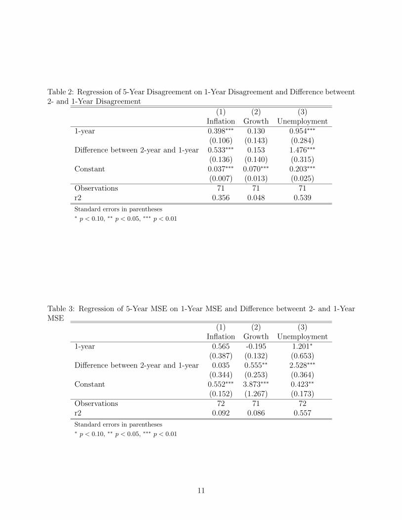
Table 2: Regression of 5-Year Disagreement on 1-Year Disagreement and Difference betweent2- and 1-Year Disagreement
(1) (2) (3)Inflation Growth Unemployment
1-year 0.398∗∗∗ 0.130 0.954∗∗∗
(0.106) (0.143) (0.284)Difference between 2-year and 1-year 0.533∗∗∗ 0.153 1.476∗∗∗
(0.136) (0.140) (0.315)Constant 0.037∗∗∗ 0.070∗∗∗ 0.203∗∗∗
(0.007) (0.013) (0.025)Observations 71 71 71r2 0.356 0.048 0.539
Standard errors in parentheses∗ p < 0.10, ∗∗ p < 0.05, ∗∗∗ p < 0.01
Table 3: Regression of 5-Year MSE on 1-Year MSE and Difference betweent 2- and 1-YearMSE
(1) (2) (3)Inflation Growth Unemployment
1-year 0.565 -0.195 1.201∗
(0.387) (0.132) (0.653)Difference between 2-year and 1-year 0.035 0.555∗∗ 2.528∗∗∗
(0.344) (0.253) (0.364)Constant 0.552∗∗∗ 3.873∗∗∗ 0.423∗∗
(0.152) (1.267) (0.173)Observations 72 71 72r2 0.092 0.086 0.557
Standard errors in parentheses∗ p < 0.10, ∗∗ p < 0.05, ∗∗∗ p < 0.01
11

Table 4: Regression of Realization at 5-Year Horizon on Realization at 1-Year Horizon andDifference betweent 2- and 1-Year Horizons
(1) (2) (3)Inflation Growth Unemployment
1-year 0.443∗∗∗ 0.314∗∗∗ 0.851∗∗∗
(0.136) (0.096) (0.041)Difference between 2-year and 1-year 1.147∗∗∗ 1.511∗∗∗ 2.949∗∗∗
(0.228) (0.338) (0.310)Constant 0.960∗∗∗ 0.883∗∗∗ 1.412∗∗∗
(0.240) (0.238) (0.421)Observations 72 71 72r2 0.370 0.457 0.908
Standard errors in parentheses∗ p < 0.10, ∗∗ p < 0.05, ∗∗∗ p < 0.01
2.2 Drivers of Long- and Short-Run Uncertainty
We regress uncertainty or disagreement at each horizon h on several potential drivers of
uncertainty and disagreement. Following Barrero et al. (2017), we consider the Economic
Policy Uncertainty (EPU) index for Europe and measures of volatility of oil price returns
and exchange rate returns. Abel et al. (2016, p. 534) find “evidence of an economically and
statistically signicant relationship between uncertainty and aggregate point predictions—a
negative association for GDP growth and a positive association for unemployment.” Thus,
we also include either the mean point forecast for inflation, growth, and unemployment or the
realization of inflation, growth, and unemployment in the previous quarter in the regressions.
(We do not include point forecasts and lagged realizations simultaneously because of high
collinearity.) In some specifications, we also include the change or squared change in inflation,
growth, and unemployment.
The EPU is based on newspaper articles regarding policy uncertainty.6 Our oil price series
is “Crude Oil Prices: Brent - Europe” from the U.S. Energy Information Administration.
We compute the standard deviation of daily returns for the past 252 trading days, which is
6Data was downloaded in April 2018 from http://www.policyuncertainty.com/europe monthly.html. Thenewspapers include Le Monde and Le Figaro for France, Handelsblatt and Frankfurter Allgemeine Zeitungfor Germany, Corriere Della Sera and La Repubblica for Italy, El Mundo and El Pais for Spain, and TheTimes of London and Financial Times for the United Kingdom.
12

Figure 5: Oil Prices and Exchange Rate
Notes:
the number in a typical year.
[TO BE DONE]
13

Figure 6: Volatility of Oil Price and Exchange Rate Returns
Notes: Volatility is the standard deviation of returns over past year (252 trading days).
14

Figure 7: Volatility and Economic Policy Uncertainty
Notes: Volatility is a weighted average of oil return volatility and exchange rate return volatility. EPU isEuropean Economic Policy Uncertainty.
15

3 Model of Information Structure and Forecast For-
mation
Following Baker et al. (2017), we use a model in which N agents forecast a m-dimensional
stationary Markov signal process πt using noisy public and private signals. The observation
process for agent i is
yt(i) =
A(i)
B
πt +
νt(i)
ηt
. (1)
where ηt and νt(i) are the public and private noise and the matrix A(i) corresponds to
the private manifestation of the signal. We assume that ηt is serially uncorrelated and—
to allow for time-varying uncertainty— has a stochastic covariance matrix Σt. The private
noises νt(i) are serially uncorrelated with deterministic covariance matrix Σ(i).
3.1 State Space Representation
We first consider the forecasters’ Kalman filtering process in the case that Σt, the parameters
governing πt, and the matrices B and A(i) are known. Later, to introduce first- and second-
moment shocks, we will consider the unknown parameters case (Refer to Baker et al. (2017)
for details).
Suppose there exists a matrix G such that πt = Gxt, where xt is a Markovian state vector
xt with transition equation:
xt = Φxt−1 + εt (2)
for t ≥ 1, with initial value x0. We assume the transition matrix Φ has eigenvalues less than
one in magnitude and that the signal innovations εt are uncorrelated with x0, so that εt
is uncorrelated with xt−1 for t ≥ 1. The innovations’ common covariance matrix is denoted
16
Σε. Let
δt(i) =
ν(i)t
ηt
H(i) =
A(i)
B
G,
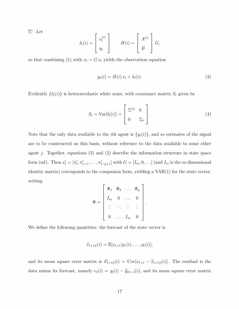
so that combining (1) with πt = Gxt yields the observation equation
yt(i) = H(i)xt + δt(i). (3)
Evidently δt(i) is heteroscedastic white noise, with covariance matrix St given by
St = Var[δt(i)] =
Σ(i) 0
0 Σt
. (4)
Note that the only data available to the ith agent is yt(i), and so estimates of the signal
are to be constructed on this basis, without reference to the data available to some other
agent j. Together, equations (3) and (2) describe the information structure in state space
form (ssf). Then x′t = [π′t, π′t−1, . . . , π
′t−p+1] with G = [Im, 0, . . .] (and Im is the m-dimensional
identity matrix) corresponds to the companion form, yielding a VAR(1) for the state vector,
writing
Φ =
Φ1 Φ2 . . . Φp
Im 0 . . . 0
.... . .
......
0 . . . Im 0
.
We define the following quantities: the forecast of the state vector is
xt+1|t(i) = E[xt+1|y1(i), . . . , yt(i)],
and its mean square error matrix is Pt+1|t(i) = Cov[xt+1 − xt+1|t(i)]. The residual is the
data minus its forecast, namely et(i) = yt(i) − yt|t−1(i), and its mean square error matrix
17

is denoted Vt(i). The Kalman gain is by definition Kt(i) = Cov[xt+1, et(i)] Var[et(i)]−1, and
plays a key role in updating a signal extraction estimate given new information. Initialization
of the recursive Kalman filter algorithm is given by x1|0(i) = 0 and P1|0(i) = Var[x1], which
are the correct quantities given a stationary state vector. In the case of a VAR(p) signal
process, this initial variance can be computed directly from the companion form. Then for
1 ≤ t ≤ T , we compute
et(i) = yt(i)−H(i) xt|t−1(i) (5)
Vt(i) = H(i)Pt|t−1(i)H(i)′ + St (6)
Kt(i) = ΦPt|t−1(i)H(i)′ Vt(i)−1 (7)
xt+1|t(i) = Φ xt|t−1(i) +Kt(i) et(i) (8)
Pt+1|t(i) = (Φ−Kt(i)H(i)) Pt|t−1(i) Φ′ +G′ΣεG. (9)
Equation (7) gives a recursive formula for the Kalman gain, and its dependence on the
heteroscedastic noise is clearly given through Vt(i) in (6). Moreover, equations (8) and (9)
tell us how to update our one-step ahead prediction and forecast error variance for the state
vector. Again, because the Kalman gain depends upon the heteroscedastic variance Σt, both
the state vector forecast and its uncertainty will be impacted. In order to obtain (k+1)-step
ahead forecasts (k ≥ 0), we compute
πt+1|t−k(i) = GΦk xt+1−k|t−k(i) (10)
Var[πt+1|t−k(i)− πt+1] = GPt+1|t−k(i)G′, (11)
where Pt+1|t−k(i) = Var[xt+1|t−k(i) − xt+1] and is further described below. So (10) provides
an optimal estimate of the forecasted signal, given the presence of noise with time-varying
volatility.
We require a flexible and broad specification for the signal and noise processes, and
18

propose the VAR(p) class for the signal, where p is taken sufficiently large to approximate a
generic signal. We parametrize this process such that stationarity is guaranteed, as described
in Roy, McElroy and Linton (2017); the private noise has variance matrix Σ(i), which can
be parameterized as a member of the space of symmetric positive definite matrices. For the
dynamics of the public signal, we describe Σt as a stochastic volatility process.7 Following
the work of Cogley and Sargent (2005), Primiceri (2005), and Neusser (2016), consider
the Cholesky decomposition Σt = Bt ΩtB′t, where Bt is unit lower triangular and Ωt is
diagonal. The diagonal entries of Ωt each follow an exponential random walk, and the
Bt = expCt, where Ct is a lower triangular with zeroes on the diagonal. Each lower
triangular element of Ct follows an independent random walk. This framework – of a VAR(p)
signal with the exponential random walk model for volatility – can be tailored to the user’s
specification through the parameter settings, which determine the dispersion for the random
walk increments in the volatility process.
A temporary shock at some time index τ can be generated by scaling the diagonal entries
of a single Σt by some a > 0, but without altering Bt or Ωt, so that the effect is transitory:
Σt = Bt ΩtB′t · (1 + a 1t=τ). (12)
This ensures that Στ has values multiplied by 1+a, but the corresponding shock ητ will not be
large unless the random vector is generated from the right tail of the normal distribution. We
proceed by generating m random variables Z independently from the marginal distribution
P[Z > x|Z > 2] = (1−Φ(x))/(1−Φ(2)), and multiplying the corresponding vector ζ by Σ1/2τ
to obtain ητ . This modification to ηt and Σt at time t = τ will be designated as temporary
first-moment and second-moment shocks.
A permanent shock at some time index τ involves dilating Σt in the same manner as the
7Chiu, Leonard and Tsui (1996) modeled Σt as the matrix exponential of a symmetric matrix At (whichcan take negative values), whose vech was modeled as a VAR process. Uhlig (1997) modeled Σt via ageneralized Cholesky decomposition, wherein the diagonal factor followed a positive random walk model. AWishart autoregressive process was studied in Gourieroux, Jasiak and Sufana (2009).
19

temporary shock, but with the effect lasting for all times t ≥ τ :
Σt = Bt ΩtB′t · (1 + a 1t≥τ). (13)
This second-moment shock is paired with a first-moment shock obtained by generating a
temporary first-moment shock ζ at time t = τ in the manner described above, and for t > τ
we draw an independent standard normal random vector υt, and set ηt = Σ1/2t (ζ+υt). Note
that in this construction, ζ corresponds to an initial up-swing at time τ , which is persistent
at later times t > τ .
4 A Framework for Expectation Formation
The key three ingredients of our framework are: (i) multi-step ahead forecasting, (ii) stochas-
tic volatility, and (iii) Kalman filter updating. The ith agent (1 ≤ i ≤ N) observes both
public and private signals and makes the forecast through a signal extraction process. Given
the data yt(i) for 1 ≤ t ≤ T , for each agent i, we obtain the (k + 1)-step ahead forecast
πt+1|t−k(i) from (10); calculation of the uncertainty relies upon Pt+1|t−k(i) in (11), which is
a special case of the multi-step ahead error covariance
R(ij)k,` (t) = Cov
[xt+1|t−k(i)− xt+1, xt+1|t−`(j)− xt+1
],
i.e., the covariance of forecast errors for the ith agent (k + 1 steps ahead) and the jth agent
(`+ 1 steps ahead). The following result provides a recursive algorithm for computing these
covariances, based upon recursions for the one-step ahead error covariances
Q(ij)t+1|t = Cov[xt+1|t(i)− xt+1, xt+1|t(j)− xt+1].
20

Note that setting j = i and ` = k we obtain Pt+1|t−k(i) = R(ii)k,k (t), and furthermore Q
(ii)t+1|t =
Pt+1|t(i).
Proposition 1 The covariance of one-step ahead prediction errors across agents, Q(ij)t+1|t,
can be computed recursively by
Q(ij)t+1|t = [Φ−Kt(i)H(i)]Q
(ij)t|t−1[Φ−Kt(j)H(j)]′ + Σε −Kt(i)
0 0
0 Σt
Kt(j)′, (14)
with the initialization Q(ij)1|0 = Var[x1] for all i and j. The covariance of prediction errors
across forecast horizons and agents, R(ij)k,` (t), can be computed if k ≤ ` by
R(ij)`,` (t) = Φ`Q
(ij)t+1−`|t−` Φ′` +
`−1∑n=0
Φn Σε Φ′n
R(ij)`−1,`(t) = Φ`−1 (Φ−Kt+1−`(i)H(i))Q
(ij)t+1−`|t−` Φ′` +
`−1∑n=0
Φn Σε Φ′n
R(ij)k,` (t) = Φk
`−1∏n=k
(Φ−Kt−n(i)H(i))Q(ij)t+1−`|t−` Φ′` +
`−k∑m=2
Φk
`−m∏n=k
(Φ−Kt−n(i)H(i)) Σε Φ′`−m+1
+k∑
n=0
Φn Σε Φ′n,
where k ≤ `− 2 in the last case, and where the matrix products are computed with the lowest
index matrix first, and multiplying on the right by matrices of higher index.
It is clear that Proposition 1 can be used to compute the mean squared error (MSE) of
multi-step ahead forecast errors, and is a new result in the state space literature of interest in
its own right. Beyond supplying the covariances needed to compute (11), the proposition also
allows us to compute aggregate forecaster MSE. If we have interest in some linear composite
of economic agents’ results, say
πt+k+1|t =N∑i=1
wi πt+k+1|t(i) (15)
21

for given weights wi, then the corresponding target is∑N
i=1wiπt+k+1, which equals πt+k+1
when the weights sum to one. The variance of the discrepancy between πt+k+1|t and πt+k+1
is the forecast MSE, given by
MSEt+k+1|t =N∑
i,j=1
wiwj GR(ij)k,k (t+ k)G′. (16)
To compute (16) recursively, for fixed k, we only need the first formula in Proposition 1,
which in turn requires us to know Q(ij)t+1|t, and is calculated from (14). The disagreement
across agents is defined as the sample variability of the forecasts across forecasters, i.e.,
Dt+k+1|t =N∑i=1
wi(πt+k+1|t(i)− πt+k+1|t
) (πt+k+1|t(i)− πt+k+1|t
)′. (17)
This is easily computed from (10) and (15). To see this, we can show that
πt+k+h+1|t(i)− πt+k+h+1|t = GΦh(xt+k+1|t(i)− xt+k+1
),
where xt+k+1 =∑N
i=1wi xt+k+1|t(i). Substituting into (17) yields
Dt+k+h+1|t =N∑i=1
wiGΦh(xt+k+1|t(i)− xt+k+1|t
) (xt+k+1|t(i)− xt+k+1|t
)′Φ′hG′,
which expresses the (h+k+1)-step ahead dispersion in terms of (k+1)-step ahead dispersion
(of the state vector).
Let the aggregate forecast uncertainty be defined as
Ut+k+1|t =N∑i=1
wi Pt+k+1|t(i),
which represents an average (across agents) of the variability in k-step ahead forecasting of
the state vector. Then we have the following result.
22

Proposition 2 The covariance of prediction errors across one forecast horizon and multiple
agents can be recursively computed via
R(ij)k+h,k+h(t+ k + h) = ΦhR
(ij)k,k (t+ k) Φ′h +
h−1∑n=0
Φn Σε Φ′n.
Hence the aggregate forecast uncertainty satisfies
Ut+k+1|t = Φk Ut+1|t Φ′k +k−1∑n=0
Φn Σε Φ′n. (18)
5 Simulation
[TO BE DONE]
6 Conclusion
In the Great Recession, professional forecasters in Europe not only became more uncertain
about inflation, growth, and unemployment, but also expressed more disagreement in their
forecasts. While disagreement has since fallen at most horizons, uncertainty remains elevat-
ed. Understanding the sources of disagreement and uncertainty is an important goal, with
implications about the social value of public information and about the effects of policies that
work partially through an expectations channel (such as monetary policy and tax policy)
(Mankiw et al., 2004).
Patton and Timmermann (2010) point out that the term structure of forecaster disagree-
ment is a way of deducing the relative importance of various causes of disagreement. They
find that greater disagreement during recessions is not due to increased heterogeneity in in-
formation signals but rather to agents putting more weight on model-based forecasts during
recessions. Similarly, analysis of the term structure of uncertainty can help reveal the causes
of uncertainty and information about forecasters’ models and beliefs.
23

References
Abel, Joshua, Robert Rich, Joseph Song, and Joseph Tracy (2016) “The Measurement and
Behavior of Uncertainty: Evidence from the ECB Survey of Professional Forecasters,”
Journal of Applied Econometrics, Vol. 31, pp. 533–550.
Acemoglu, Daron, Victor Chernozhukov, and Muhamet Yildiz (2016) “Fragility of asymp-
totic agreement under Bayesian learning,” Journal of Theoretical Economics, Vol. 11, pp.
187–225.
Andrade, Philippe, Richard Crump, Stefano Eusepi, and Emanuel Moench (2016) “Funda-
mental Disagreement,” Journal of Monetary Economics, Vol. 83, pp. 106–128.
Bachmann, Rudiger and Christian Bayer (2013) “Wait-and-See Business Cycles?” Journal
of Monetary Economics, Vol. 60, pp. 704–719.
Bachmann, Rudiger, Steffen Elstner, and Eric Sims (2013) “Uncertainty and Economic Ac-
tivity: Evidence from Business Survey Data,” American Economic Journal: Macroeco-
nomics, Vol. 5, pp. 217–249.
Baker, Scott and Nicholas Bloom (2013) “Does Uncertainty Reduce Growth? Using Disasters
as Natural Experiments,” NBER Working Paper No. 19475.
Baker, Scott, Nicholas Bloom, and Steven Davis (2016) “Measuring Economic Policy Uncer-
tainty,” Quarterly Journal of Economics, Vol. 131, pp. 1593–1636.
Baker, Scott, Tucker McElroy, and Xuguang Sheng (2017) “Expectation Formation Following
Large Unexpected Shocks,” Mimeo.
Ball, Laurence and Stephen Cecchetti (1990) “Infation and Uncertainty at Short and Long
Horizons,” Brookings Papers on Economic Activity, Vol. 1, pp. 215–254.
Barrero, Jose Maria, Nicholas Bloom, and Ian Wright (2017) “Short and Long Run Uncer-
tainty,” NBER Working Paper No. 23676.
24

Binder, Carola (2017a) “Economic Policy Uncertainty and Household Inflation Uncertainty,”
B.E. Journal of Macroeconomics.
(2017b) “Measuring Uncertainty Based on Rounding: New Method and Application
to Inflation Expectations,” Journal of Monetary Economics, Vol. 90, pp. 1–12.
Bloom, Nicholas (2009) “The Impact of Uncertainty Shocks,” Econometrica, Vol. 77, pp.
623–685.
(2014) “Fluctuations in Uncertainty,” Journal of Economic Perspectives, Vol. 28,
pp. 153–176.
Bloom, Nick, Stephen Bond, and John Van Reenen (2007) “Uncertainty and Investment
Dynamics,” Review of Economic Studies, Vol. 74, pp. 391–415.
Boero, Gianna, Jeremy Smith, and Kenneth Wallis (2008) “Uncertainty and disagreement
in economic prediction: the Bank of England Survey of External Forecasters,” Economic
Journal, Vol. 118, pp. 1107–1127.
Coibion, Olivier and Yuriy Gorodnichenko (2012) “What can survey forecasts tell us about
information rigidities?” Journal of Political Economy, Vol. 120, pp. 116–159.
D’Amico, Stefania and Athanasios Orphanides (2008) “Uncertainty and Disagreement in
Economic Forecasting,” Finance and Economics Discussion Series, Board of Governors
of the Federal Reserve System, Vol. 56, pp. 1–35.
Dixit, Avinash and Robert Pindyck (1994) Investment under Uncertainty, Princeton, NJ:
Princeton University Press.
Dovern, Jonas, Ulrich Fritsche, and Jiri Slacalek (2012) “Disagreement among Forecasters
in G7 Countries,” Review of Economics and Statistics, Vol. 94, pp. 1081–1096.
Gali, Jordi (2015) “Hysteresis and the European Unemployment Problem Revisited,” NBER
Working Paper No. 21430.
25

Giacomini, Raffaella, Vasiliki Skreta, and Javier Turen (2016) “Models, Inattention and
Bayesian Updates,” Mimeo.
Hellwig, Christian and Venky Venkateswaran (2009) “Setting the right prices for the wrong
reasons,” Journal of Monetary Economics, Vol. 56, pp. 557–577.
Kandel, Eugene and Neil Pearson (1995) “Differential interpretation of public signals and
trade in speculative markets,” Journal of Political Economy, Vol. 103, pp. 831–872.
Lahiri, Kajal and Xuguang Sheng (2008) “Evolution of Forecast Disagreement in a Bayesian
Learning Model,” Journal of Econometrics, Vol. 144, pp. 325–340.
(2010) “Measuring Forecast Uncertainty by Disagreement: The Missing Link,”
Journal of Applied Econometrics, Vol. 25, pp. 514–538.
Leduc, Sylvain and Zheng Liu (2016) “Uncertainty Shocks are Aggregate Demand Shocks,”
Journal of Monetary Economics, Vol. 82, pp. 20–35.
Mankiw, N. Gregory, Ricardo Reis, and Justin Wolfers (2004) “Disagreement about Inflation
Expectations,” in Mark Gertler and Kenneth Rogoff eds. NBER Macroeconomics Annual,
Vol. 18: MIT Press.
Patton, Andrew and Allan Timmermann (2010) “Why do forecasters disagree? Lessons from
the term structure of cross-sectional dispersion,” Journal of Monetary Economics, Vol. 57,
pp. 803–820.
Rich, Robert and Joseph Tracy (2010) “The relationships among expected inflation, dis-
agreement, and uncertainty: evidence from matched point and density forecasts,” Review
of Economics and Statistics, Vol. 92, pp. 200–207.
Varian, Hal (1985) “Divergence in Opinion in Complete Markets: A Note,” Journal of
Finance, Vol. 40, pp. 309–317.
26
Wieland, Volker and Maik Wolters (2011) “The Diversity of Forecasts from Macroeconomic
Models of the U.S. Economy,” Economic Theory, Vol. 47, pp. 247–292.
Woodford, Michael (2001) “Imperfect Common Knowledge and the Effects of Monetary
Policy,” in Philippe Aghion, Roman Frydman, Joseph Stiglitz, and Michael Woodford
eds. Knowledge, Information, and Expectations in Modern Macroeconomics: In Honor of
Edmund S Phelps: Princeton University Press.
Wright, Ian (2015) “Firm Investment and the Term Structure of Uncertainty,” Stanford
Institute for Economic Policy Research Working Paper.
Zarnowitz, Victor and Louis A. Lambros (1987) “Consensus and Uncertainty in Economic
Prediction,” Journal of Political Economy, Vol. 95, pp. 591–621.
27

Appendix A Tables and Figures
Table A.1: Variables Forecasted by the European Central Bank Survey of Professional Fore-casters
Name Notation DescriptionInflation π Year on year percentage change of the Harmonised Index
of Consumer Prices (HICP) published by Eurostat
Growth g Year on year percentage change of real GDPbased on ESA definition
Unemployment u Unemployment as percentage of labor forcebased on Eurostat definition
Notes: For more information, see “ECB Survey of Professional Forecasters (SPF): Description of SPFDataset.”
Table A.2: Survey Return Dates and Available Information
Quarter Return Date Last π Obs. Last g Obs. Last u Obs.1 Late Jan/early Feb Dec Q3 Nov2 Late April/early May March Q4 Feb3 Late July/early Aug June Q1 May4 Late Oct/early Nov Sep Q2 Aug
Notes: For more information, see “ECB Survey of Professional Forecasters (SPF): Description of SPFDataset.”
28

Appendix B Proofs
Proof of Proposition 1 Equation (14) was proved in Proposition 1 of Baker et al.(2017). The multi-step ahead forecasting of the state vector is straightforward: xt+1|t−k(i) =
Φk xt+1−k|t−k(i). Also, iteration of (2) yields xt+1 = Φk xt+1−k +∑k−1
n=0 Φn εt+1−n. Thereforethe multi-step ahead forecasting error can be expressed in terms of one-step ahead forecastingerror, via
xt+1|t−k(i)− xt+1 = Φk(xt+1−k|t−k(i)− xt+1−k
)−
k−1∑n=0
Φn εt+1−n.
We can also express the one-step ahead forecasting error in terms of prior such errors.Suppose k < `:
xt+1−k|t−k(i)− xt+1−k = Φ(xt−k|t−k−1(i)− xt−k
)+Kt−k(i) et−k(i)− εt−k+1
· · · = Φ`−k (xt+1−`|t−`(i)− xt+1−`)
+`−k−1∑n=0
Φn (Kt−k−n(i) et−k−n(i)− εt+1−k−n) .
This indicates that the multi-step ahead forecasting error is related to past one-step aheadforecasting errors as follows, when k < `:
xt+1|t−k(i)−xt+1 = Φ`(xt+1−`|t−`(i)− xt+1−`
)−`−1∑n=0
Φn εt+1−n+`−k−1∑n=0
Φn+kKt−k−n(i) et−k−n(i).
The errors et(i) have the following form:
et−k−n(i) = yt−k−n(i)−H(i) xt−k−n|t−k−n−1(i) = −H(i)(xt−k−n|t−k−n−1(i)− xt−k−n
)+δt−k−n(i).
(19)For 0 ≤ n ≤ ` − k − 1, δt−k−n(i) is uncorrelated with xt+1−`|t−`(i) − xt+1−`, and moreoverfor 0 ≤ n ≤ `− 1, εt+1−j is uncorrelated with xt+1−`|t−`(i)− xt+1−`. Now using (19), we canre-express the one-step ahead forecasting errors as
xt+1−k|t−k(i)− xt+1−k = (Φ−Kt−k(i)H(i))(xt−k|t−k−1(i)− xt−k
)+Kt−k(i) δt−k(i)− εt−k+1
· · · =`−1∏n=k
(Φ−Kt−n(i)H(i))(xt−`+1|t−`(i)− xt−`+1
)+
`−2∏n=k
(Φ−Kt−n(i)H(i)) (Kt−`+1(i) δt−`+1(i)− εt−`+2)
· · ·+ (Φ−Kt−k(i)H(i)) (Kt−k−1(i) δt−k−1(i)− εt−k) +Kt−k(i) δt−k(i)− εt−k+1.
29
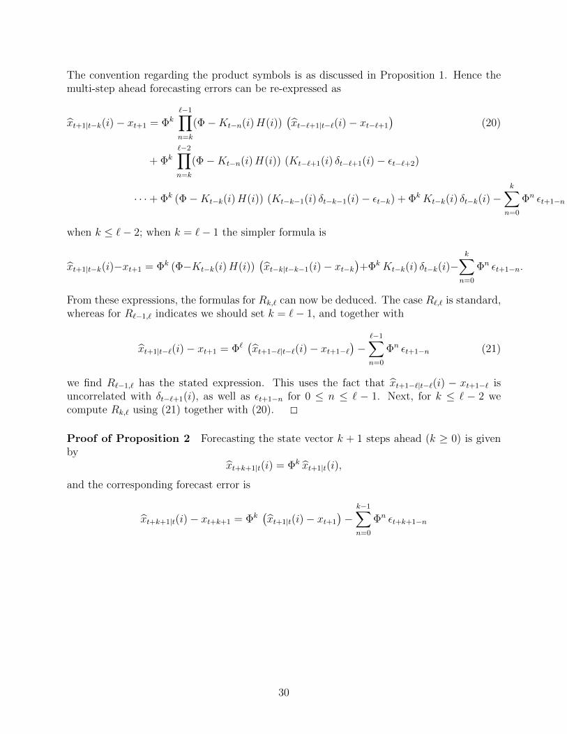
The convention regarding the product symbols is as discussed in Proposition 1. Hence themulti-step ahead forecasting errors can be re-expressed as
xt+1|t−k(i)− xt+1 = Φk
`−1∏n=k
(Φ−Kt−n(i)H(i))(xt−`+1|t−`(i)− xt−`+1
)(20)
+ Φk
`−2∏n=k
(Φ−Kt−n(i)H(i)) (Kt−`+1(i) δt−`+1(i)− εt−`+2)
· · ·+ Φk (Φ−Kt−k(i)H(i)) (Kt−k−1(i) δt−k−1(i)− εt−k) + ΦkKt−k(i) δt−k(i)−k∑
n=0
Φn εt+1−n
when k ≤ `− 2; when k = `− 1 the simpler formula is
xt+1|t−k(i)−xt+1 = Φk (Φ−Kt−k(i)H(i))(xt−k|t−k−1(i)− xt−k
)+ΦkKt−k(i) δt−k(i)−
k∑n=0
Φn εt+1−n.
From these expressions, the formulas for Rk,` can now be deduced. The case R`,` is standard,whereas for R`−1,` indicates we should set k = `− 1, and together with
xt+1|t−`(i)− xt+1 = Φ`(xt+1−`|t−`(i)− xt+1−`
)−
`−1∑n=0
Φn εt+1−n (21)
we find R`−1,` has the stated expression. This uses the fact that xt+1−`|t−`(i) − xt+1−` isuncorrelated with δt−`+1(i), as well as εt+1−n for 0 ≤ n ≤ ` − 1. Next, for k ≤ ` − 2 wecompute Rk,` using (21) together with (20). 2
Proof of Proposition 2 Forecasting the state vector k + 1 steps ahead (k ≥ 0) is givenby
xt+k+1|t(i) = Φk xt+1|t(i),
and the corresponding forecast error is
xt+k+1|t(i)− xt+k+1 = Φk(xt+1|t(i)− xt+1
)−
k−1∑n=0
Φn εt+k+1−n
30
(where the sum is omitted if k = 0). So for h > 0, we obtain
xt+k+h+1|t(i)− xt+k+h+1 = Φh+k(xt+1|t(i)− xt+1
)−
h+k−1∑n=0
Φn εt+k+1−n
= Φh
Φk(xt+1|t(i)− xt+1
)−
k−1∑n=0
Φn εt+k+1−n
−
h−1∑n=0
Φn εt+h+k+1−n
= Φh(xt+k+1|t(i)− xt+k+1
)−
h−1∑n=0
Φn εt+h+k+1−n.
The two terms on the right hand side are uncorrelated with one another, and hence we obtainthe relation (18). Next, setting h = 0 and using Pt+k+1|t(i) = R
(ii)k,k (t+k) and summing against
wi (which sum to one), we obtain the recursive relation for aggregate forecast uncertainty.2
31