Terminology in Digital Signal Processin - UC Santa … in Digital Signal Processin LAWRENCE R. RABINER, JAMES W. COOLEY, HOWARD D. HELMS, LELAND B. JACKSON, JAMES F ... In digital

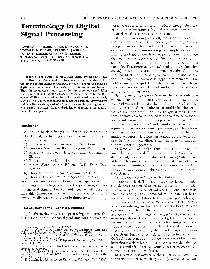
Terminology in Digital Signal Processin

LAWRENCE R. RABINER, JAMES W. COOLEY, HOWARD D. HELMS, LELAND B. JACKSON, JAMES F. KAISER, CHARLES M. RADER, RONALD W. SCHAFER, KENNETH STEIGLITZ, and CLIFFORD J. WEINSTEIN

Absfract-The committee on Digital Signal Processing of the IEEE Group on Audio and Electroacoustics has undertaken the project of recommending terminologg for use in papers and texts on digital signal processing. The reasons for this project are twofold. First, the meanings of many terms that are commonly used differ from one author to another. Second, there are many terms that one would like to have defined for which no standard term currently exists. It is the purpose of this paper to propose terminology which we feel is self-consistent, and which is in reasonably good agreement with current practices. An alphabetic index of terms is included at the end of the paper.

Introduction

As an aid to classifying the different types of terms to be defined, we have placed each term in one of the following groups:

1) Introductory Terms-General Definitions 2) Discrete Systems-Block Diagram Terminology- 3) Relations Between Discrete and Continuous

4) Theory and Design of Digital Filters 5) Finite Word Length Effects-A/D, D/A Con-

6) Discrete Fourier Transforms and the FFT 7) Discrete Convolution and Spectrum Analysis.

Signals

version

In the above mentioned sections of this paper we will be discussing terminology related to the processing of one- dimensional signals. For convenience, we will assume that this dimension i s time-although the definitions apply equally well to any single dimension.

1. introductory Terms-General Definitions

1) In discussing waveform processing problems, the distinctions analog versus digital and continuous time

Manuscript received August 1, 1972. L. R. Rabiner, J. F. Kaiser, and R. W. Schafer are with Bell

J . W. Cooley is with the I B M T. J. \&’atson Research Center,

H. D. Helms is with Bell Telephone Laboratories, Inc., Whip-

Telephone Laboratories, Inc., Murray Hill, N . J . 07974.

Vorktown Heights, 73. Y. 10598.

pany, N . J . 07981.

Nyack, N. 1’. 10994. I,. B. Jackson is with Rockland Systems Corporation, West

C. M. Rader and C. 1. Weinstein are with M.I.T. Lincoln Lab- oratory, Lexington, Mas:. 02173. (Operated with support from the U. S. Air Force.)

K. Steiglitz is with Princeton University, Princeton, pi. J . 08540.

versus discrete time are often made. Although they are often used interchangeably, different meanings should be attributed to the two sets of terms.

2) The term analog generally describes a waveform that is continuous in time (or any other appropriate independent variable) and that belongs to a class that can take on a continuous range of amplitude values. Examples of analog wuveJorms or anulog signals are thosc derived from acoustic sources. Such signals are represented rnathematically as functions of a continuous variable. The functions sin (ut) and the step function au-l(t) are examples of common mathematical functions that could describe “analog signals.” The use of the term “anaIog” in this context appears to stem fronl the field of analog computation, where a current or voltage waveform serves as a physical analog of some variable in a differential equation.

3 ) The term continuous t ime implies that only the independent variable necessarily takes on a continuous range of values. I n theory the amplitude may, but need not, be restricted to a finite or countable infinite set of values (i.e., the amplitude may be quantized). There- fore, analog waveforms are continuous-time waveforms with continuous amplitude. In practice, however, “continuous-time waveforms” and “analog waveforms” are equivalent. Since most signal processing problems have nothing to do with analogs as such, the us11 of the term analog waveform is often ambiguous at the least and may in fact be misleading. T ~ L I S , the term continuous- time waveform is preferable.

4) Discrete time implies that time (the independent variable) is quantized. T h a t is, discrete-time signals are defined only for discrete values of the independent variable. Such signals are represented rnathcmatically as sequences of numbers. Those discrete-time signals that take on a continuum of values are referred t o as sum$led- data signals.

5 ) The term digital implies that lmth timc and mlpli-- tude are quantized. Thus a digital system i s one i n w h i c h signals. are represented as sequences o f n u m h - r s which take on only a finite set of values. Thlls onc uses d ig i td when discussing actual phJ-sical realizations (as hardware or programs) o f discrete-time signal processing systems, whereas the term discrete t i m e is a h;tt-er modifier when considering mathematical abstractions of such systems in which the effects of amplitud- quantization are ignored, A digital signal or digital ~ ( ~ v e j o s m is a sc- quence produced, for example, b y digital circuitry or by an analog-to-digital converter which is sampling a COIF

tinuous-time waveform. In digital signal processing these terms are commonly shortened to signal 01- wave- f o rm. Sometimes the term signal is restricted to being a desirable component of a sequence instead of being used interchangeably with waveform. Noise is either defined as a) an undesirable component of a sequence, or b) a sequence of random variables.

6 ) (Digital) simulatiofz i s the exact or approxinlate representation o f a given system (discrete or contin-

IaBIirTm et al.: DIGITAL SIGKAL PROCESSING TERMIXOLOGY 323

uous) called the source system, by a (digital) system y ( n ) = x ( n - m), m > 0 (2) called the object system.

7) Next-state simulation is a method of digital simulation whereby the values of the digital system signals

m

( 3 )

are represented by nodes in a block diagram representation. Usually, there is a close correlation between blocks in the object system and elements of the source system. The method entails ordering the calculations in the digital system so that all the inputs to each block a t a given sample time are computed before the output is computed.

8) A real-time process is one for which, on the average, the computing associated with each sampling interval can be completed in a time less than or equal to the sampling interval. ,4 program running in 100 times real time requires 100 times as long to process the Sam(: number of samples; i.e., it is 100 times too slow for real time operation. A program ten times as fast as it needs to be could be said to run in 1/10 real time. Obviously, the extra speed can only be used if other computing can be done in the interstices, or if the complete sequences to be processed have been stored beforehand.

9) Throughp.ut rate is the total rate at which digital information is processed by a discrete-time system, measured in bits per second or samples per second. In a multiplexed system, where several signals are processed, we may refer to the throughput rate per signal, measured in bits per second per signal or samples per second per signal. Thus, a multiplexed system which processes 10 signals, each at 1000 bits/s, has a throughput rate of 10 000 bits/s, and a throughput rate/signal of 1000 bits/s/signal.

10) A multivate system is a discrete-time system in which there are signals sampled a t different intervals which are usually integer multiples of some basic or fundamental interval.

In ( 3 ) , X ( z ) appears multiplied by z-%. This result for m'= 1 accounts for the fact that 2-l is often termed the unit delay operator, since a delay of the sequence by one sample is equivalent to multiplication of the z transform by z- l . ( Similarly, z is often called the unit advance operator.)

2) In many cases, sequences are defined over both positive and negative values of A. In such cases, a some- what more general point of view is called for. In general, the z transform is written as

m

X ( Z > = x(n)z-a. (4) n=--m

I t should be noted that a common usage is to call (1) simply the z transform, and (4) the two-sided z transform. Since (4) is most general, it would seem preferable to refer to (4) as the z transform, and the special case, ( l ) , as the one-sided z transform.

3 ) I t is possible to think of the z transform as simply a formal series whose properties can be tabulated, and which never need be summed. However, it is generally preferable to realize that if certain convergence conditions are met, both (1) and (4) are Laurent series in the complex variable z. As such, all the properties of the Laurent series apply. For example, if the series in (1) converges, it must converge in a region I zI > R+. If the series of (4) converges, it must converge in an annular region R+ < I zI < R-, where R+ may be zero and R- may be infinity. The coefficients of a Laurent series are determined by an integral relationship. In the context of the z transform, this relation is

11. Discrete Systems (5)

1) The z transform plays a role in discrete-time system theory analogous to that of the Laplace transform in continuous-time system theory. Two view points re- garding the z transform are common. One is based on what may be termed the one-sided z transform, which is defined as

m

X ( Z ) = x(n1z-n (1) 9L-0

regardless of the value of x(n) for n < 0.l One applica- tion of the one-sided z transform'is in the solution -of linear difference equations with constant coefficients. Solutions are obtained for the interval Osn < ~0 subject to prescribed initial conditions. These solutions are obtained with the aid of the equations

The notation x(%) is used rather than X,, or x(nT) to denote a sequence because of the ease of handling complicated indices, e.g., ~ ( N - 1 / 2 ) .

where C is a closed contour inside the region of convergence of the power series and enclosing the origin. Equa- tion (5) is referred to as the inverse z transform. 4) In the region of convergence of the series, both (1)

and (4) represent analytic functions of the complex variable z. These functions can often be extended by analytic continuation everywhere except at certain .singular points (poles). Since these singularities of the z transform are characteristic of the particular sequence, i t is common t,o plot their locations in the z plane, (Le., the complex plane determined by the real and imaginary parts of c). I t should be noted that it is often convenient, because of the special functional form which characterizes exponential sequences, to plot singularities in the 2-l plane. Furthermore, some authors define the z transform as

8 ( z ) = x(n)zn. (6 ) m

n=-w

324 IEEE TRANSACTIONS ON AUDIO AND ELECTROACOUSTICS, DECEMBER 1972

Clearly, (6) is related to our definition by

X ( z ) = X(z-1). (7)

If either (6) or the z-l plane is encountered, i t is a simple matter to replace z with z-l in order t o relate the z-transform definitions and to note that the region inside the unit circle of the z plane corresponds to the region outside the unit circle of the z-l plane.

5 ) A discrete-time impulse at k = k o is a discrete-time signal x ( k ) such that x ( k ) = 0 unless k = ko, in which case x ( k ) = 1. This is an analogy with an impulse at time t o in the continuous-time case, where x(/) = 6( t - t0 ) , the Dirac delta function. The response of a digital filter to a discrete-time impulse a t k = 0 is called its impulse response, or sometimes, the unit sample response. Other terms generally used for digital impulse are unit sample, unit pulse, or simply impulse.

6) A sample value is the value or number associated with one member of a sequence that represents a discrete-time signal. This term is generally used regardless of whether or not the value represents a sample of a continuous-time signal.

7) A discrete-time linear time-invariant system or a discrete-time linear filter is characterized by its impulse- response sequence h ( n ) .

8) Discrete-time convolution is the operation on a signal or sequence g(n) by the impulse response sequence h(n) to yield a digital signal (or sequence)f(n) ; the operation is defined by the expression

m

f ( ? Z ) = h(lz)g(n - Irz). (8 ) k=-m

This expression is the discrete-time counterpart of the convolution integral for continuous-time systems.

9) An alternate characterization of a discrete-time linear system is the z transform of h(n ) :

m

H ( z ) = h(n)z-n. (9) n---m

The complex function H ( z ) is called the sys t em fund ion or transfer function. The values taken by H(z) when evaluated on the unit circle in the z plane give the frequency response. Each point on the unit circle, characterized by its angle only, corresponds to a particular frequency.2 Several different units of frequency are in common use. Some authors express frequency in the conventional units of Hz, kHz, etc. Others use a system of rad/s. Still other authors use a normalized frequency with each frequency expressed as a fraction of the sampling frequency (f/fg) or half the sampling frequency (f/(f8/2)). Finally, some authors express the normalized frequency in rad/sample. The following table relates the

units of frequency to the corresponding angle in the z-plane ( T = l/fs is the sampling period).

z-Plane Unit of Frequency Substitution Around Unit Circle

Range of Frequency

When the frequency response is expressed in polar form, its magnitude as a function of frequency is called the amplitude response, and its angle as a function of frequency is called the phase response.

10) One class of linear time-invariant discrete-time filters is characterized by system functions of the form

k=l

Such filters have a recursive reali.zation in the form of the difference equation

IC= 1 k c 0

where y is the output sequence and x is the input sequence. The system function is generally written in terms of powers of z-l as in (10) because i t places in evidence the form of the difference equation given in (1 l), i.e., in terms of delays. H(z ) can also be written as

where i t is assumed that the zeros of the numerator [zeros of H ( z ) ] are distinct from the zeros of the denominator [poles of H ( z ) ] . This form places in evidence the fact that regardless of the relative values of M and N, H(z ) has the same number of poles as zeros. In most cases-especially digital filters derived from analog designs-M will be less than or equal to N , and there will be a t least N- M zeros a t z = 0. Systems of this type are called Nth-order systems. When M> N , the order of the system is no longer unambiguous. Here, N gives the order as the term is used to characterize the mathematical properties of the difference equations. M gives the order used to characterize the complexity of a realization of the system. There is no general agreement as to

As will be clear from the discussion i n Section 111, each point on .ivllicll of M or iv best characterizes the system the unit circle, i n fact, corresponds to an infinite set of uniformly spaced frequencies that are indistinguishable i n a digital system. M > N .

RABINER et ul.: DIGITAL SIGNAL PROCESSING TERMINOLOGY 325

U N I T D E L A Y y ( n ) Z x ( n - 1 1

AOOER / SUBTRACTOR r ( n ) = x ( n ) + y ( n )

CONSTANT MULTIPLIER y ( n ) = k, x ( n )

MULTIRATE DELAY ( r IS THE SAMPLING

BRANCHING OPERATION f

MULTIPLYING TWO SIGNALS r ( n ) = x ( n ) . y ( n )

y ( n 1

Fig. 1. Recommended terminology for use in block diagrams of digital systems.

11) Since the purpose of a block diagram is to graphi- cally depict the way in which a particular system is realized, the terminology shown in Fig. 1 is recommended.

111. Relations Between Discrete and Continuous Signals

1) If a sequence arises as the result of periodic sampling of a continuous-time signal x c ( t ) , i.e., x ( % ) =xc(nT) where T is the sampling period, then X ( z ) , the z transform of x(n), is related to X c ( s ) , the Laplace transform of xo( t ) by the relationship

Fig. 2. The mapping of the s plane to the z plane implied by sampling a continuous-time signal.

uridth 2 r / T , each of which maps into the entire z plane. The contributions from each strip are added to produce

2) The j axis of the s plane corresponds to the unit circle of the z plane. For this reason, the point z = 1 is often casually referred to as the DC point since it corresponds to the point s = 0 of the s plane. The z transform evaluated on the uni t circle (I z I = 1) is of particular interest in digital filtering of sampled signals. For example, there are some sequences for which the z transform does not converge (does not exist) except on the unit circle, e.g., the ideal lowpass digital filter and the ideal digital differentiator for band-limited waveforms. The z transform evaluated on the unit circle is called the Fourier transform of the sequence. This definition is consistent with the classical terminology for continuous-time systems. Evaluating (4) and ( 5 ) of Section I1 on the unit circle, yields

X ( z ) .

m

X(@) = x(nle-j.8 ( 14) ?&==--a,

This pair of equations is a Fourier transform pair for the sequence x ( % ) . Alternatively, any of the frequency units of the table in Section I1 can be used in place of 8.

3 ) If a continuous-time waveform, x c ( t ) , is band- limited to a frequency f o , i.e., X,(j27rf), the Fourier transform of x c ( t ) , is zero for I f / > f a , then xc( t ) can be recovered exactly from its samples, i.e., xc(nT), - co <n< m if T<1/2fo. This is clear from (13) where we can see that

326 IEEE TRAXSACTIOKS ON AUDIO AND ELECTRO.~COUSTICS, DECEMBER 1972

is called the sampling interval. The highest frequenq- present in x , ( t ) , (defined above) S o , is called the Nypuist frequency. The Nyquist frequency is sometimes called the folding frequency. I t is recommended that the term Nyquist frequency be avoided because of the general confusion with the term Nyquist rate. Furthermore, we recommend that the term folding frequency refer to half of the actual sampling frequency (see Fig. 3).

4) The relationship (13) between the Fourier transform of a sequence of samples x,(nT) and the Fourier transform of the continuous time signal xc( t ) is depicted in Fig. 4. Part (a) of this figure depicts a band-limited Fourier transform X , ( j 2 ~ f ) . In Fig. 4(b) and (c) the sampling rate is greater than or equal to the Nyquist rate and we note that the form of X,( j27rf) is preserved to within a constant multiplier 1/T in the frequency range - l / Z T < f < l / 2 T . However, in Fig. 4(d) the signal x,(t) is undersumpled, i.e., sampled at a rate below the Nyquist rate. In this case the Fourier transform of the sequence obtained by sampling is not equal to X,( j27rf)lT due to the fact that some of the other terms in (13) such as Xc(j27rf-j(27r/T)) are nonzero in the frequency range - 1/2T<Ip< 1/2T. One way of viewing this is to say that a set of frequencies in X,( j271-f‘) is indistinguishable from a different set of frequencies in X,( j21rj-j27r/T). These frequencies are called aliases of one another and the process of confounding frequencies as in Fig. 4(d) is called aliasing.

5 ) Suppose we have a sampled waveform x ( n ) with z transform X ( z ) . We define a new sampled waveform y ( n ) using one of every M samples as the samples of the new waveform, i.e., y ( n ) = x ( M n ) , with 13-6 any positive integer. Clearly, this process is equivalent to sampling a t a lower rate, and i t is to be expected that aliasing may occur. When the aliasing occurs due to “sampling” a discrete-time signal i t is called digital aliasing. I t is readily shown that Y(z) can be written in terms of X ( z ) as

1 M-I

M 2=0

y(z ) = - x ( z l / . ~ f e - j ( z x / ~ w ) z 1. (16)

IV. Theory and Design of Digital Filters

1) Discrete filters may be divided into two classes on the basis of whether the signal values can take on a continuum of values (sampled-data filters) or a finite set of values (digital filter). Thus we have the following.

a) A sampled-dala fi l ter i s a computational process or algorithm by which a sampled-data signal acting as an input is transformed into a second sampled-data signal termed the output. The sampled-data signal is considered only a t a set of points (usually equally spaced in time or space as the independent variable); at these points the signal can take on a continuum of values.

’ . b) A digitul filter is a computational process or algorithm by which a digital signal or sequence of num-

- fS - - f, -2fo -f, 0 f, 2f0 fs fs f

2

NYQUIST ’ .f FREQUENCY

NYQUIST RATE

SAMPLING FREQUENCY

t FOLDING FREQUENCY

Fig. 3. Labeling of terminology concerned with frequencies related to the sampling process.

- f S fS 2

(b)

- f, 0 f, I 3 fo 2f,=f,

(c)

f s = Zf,

f, < 2f,

ALIASING

(a) Fig. 4. An example of the effects of various sampling frequencies on

the frequency response of the digital signal.

hers (acting as input) is transformed into a second sequence of numbers termed the output digital signal. The numbers are limited to a finite precision. The algorithm may be implemented in software as a computer SUI,- routine for a general-purpose machine or in hardware as a special-purpose computer. The term digital filter is then applied t o the specific routine in execution or to the hardware.

2 ) Further complexity of filtering action may he obtained by switching. Thus, a switched filter ,is one .ill

RABINER et Ut. : DIGITAL SIGNAL PROCESSING TERYINOLOGY 327

which the input and output are simultaneously switched in a definite pattern among a group of input and output ports. The filter being switched may be either of the continuous or discrete types. Examples of switched filters are commutating filters or n-path filters.

3 ) A multiplexed Jilter is a restricted form of a switched filter; commonly a single discrete filter which Fig. 5. Block diagram representation of comb filter. by means of a switching action is made to perform the function of several discrete filters virtually simul- 12) A frequency-sampling Jilter is an F I R filter which taneously. Th:: multiplexing is most commonly done in is designed by varying one or of its D F T ~ coeffi- a time-division manner whereby the input to the dis- cients (called frequency samples) to minimize crete filter is sequentially switched from a number of aspects of the filter?s frequency response. F~~ example, input signals and the filter output sequentially switched the DFT coefficients of a frequency-sampling lowpass in synchronism to a corresponding set of output signal filter are 1.0 in the passband, 0.0 in the stopband, and lines. Thus a single filter may be made to do the work variable in the transition band. one design criterion of many filters by this time division multiplexing. would be to choose the variable coefficients to minimize

realized via a recursion relation, i.e., the output samples 13) extraripfile f i l t er (also called ripple of the filter are explicitly determined as a weighted sum filter) is an FIR filter whose frequency response is equi-

4) A recursive filter is a discrete-time filter which is peak stopband ripple.

of Past output saInPles as We'' as Past and/or Present ripple in both the passband and stopband, and whose input samples. For exaInPle, Y(n) =box(%) + h l x ( f l - l l ) frequency response contains the maximum possible +b2x(n-2) - a a l y ( n - l ) --2y(n-2). number of ripples6 There is no general agreement as to

5) A nonrecursive filter is a discrete-time filter for the appropriateness of this term, and as no recorn- which the output samples of the filter are explicitly mendation as to its usage is made. determined as a weighted sum of past and present input 14) equiripple (optimal) filter is an FIR filter wllich

+bzx(n - 2). to some specified frequency response characteristic over

whose impulse response h(n) is zero outside some finite lowpass filter the filter may be an extra-

samples only. For example, Y(n> =bOx(n)+blx(n-ll) is the unique best approximation in the minimax sense

6 , A finite imfiulse is a any closed subset of the frequency interval. For the

limits, i.e., h(n) = O , for n>N1 and n<N2 With N12 NZ. ripple filter, an equiripple filter with one less than the 7) An in$nite ('IR) is a maximum possible number of ripples, or a filter with the

for .which either NI = a or N2 = - or both, in 6). Thus maximum possible number of ripples all except one of the duration of the filter's impulse response is infinite. which are of equal amplitude.

restricted to z = 0 or z = a, whereas there are no such realization of an FIR filter of duration samples as a restrictions on the positions of either the poles or zeros cascade of a comb filter and a parallel bank of of I IR filters. plex pole resonators. The filter output is obtained as a

9) The terms recursive and nonrecursive are recom- weighted sum of the outputs of each of the parallel mended as descriptions for how a filter is realized and branches; thk multiplier On the Kth branch being the kth not whether or not the filter impulse response is of finite DFT coefficient of the filter impulse response. duration. (Although I IR filters are generally realized 16) A Ka~man filter (discrete time) is a linear, but

8 ) I t should be noted that the poles of F I R filters are 15) A fyequency-sampling realization is a means of

recursively, and are generally non- possibly time-varying discrete-time filter with the prop- recursively, I I R filters can be realized nonrecursively erty that it provides a least mean-square estimate and FIR filters can be realized recursively.) of a (possibly vector-valued) discrete-time signal based

lo) A t ra~sversa l filter is a (either continuous or on noisy observations. The statistical description of the discrete) in Which the output signal is generated by problem is such that the Kalman filter has a recursive

weighted by a set Of weights termed the tap gains- If the servations and old The filter design may be signal are by a tapped delay line based on a more general criterion, using a non-

summing a series of delayed versions of the input signal implementation, using a linear combination of new ob-

then the filter is termed a tapped delay line filter. quadratic loss function. Its essential features are that its design is based on a statistical criterion in the time

Or difference Of input and Output Of a Of domain, and that it is, in general, time varying. If the units and unit gain yielding a transfer characteristic filter is further restricted to be time invariant i t becomes H(z) = 1 k z--*' (see Fig. 5 ) ; this filter has hi" zeros of the Wienerfilter. transmission equally spaced on the unit circle in the

11) A JiZter is a comprised Of the sum

z plane thus giving rise t o a frequency characteristic having M equal peaks and Af real frequency zeros.

See Section VI-1 for a definition of DFT. See Section IV-29 for a definition of ripple.

328 IEEE TRANSACTIONS O S AUDIO AND EI.ECTROSCOUS?’ICS. DECEMBER 1972

...e t bN

Fig. 6. Block diagram representation of direct form 1 for an Nth-order system.

17 ) ‘The forms for realizing digital filters include the following:

a ) Direct f o r m 1 (shown in Fig. 6) where

biz-’ ’Y

& - I

i=O

For convenience in showing the realization, the order of the numerator and denominator are set to be the same. Direct form 1 uses separate delays for both the numerator polynomial and the denominator polynomial. In certain cases, e.g., floating-point additions, the results may depend on the exact ordering i n n;hich the additions are performed.

b) Direct form 2 is sho\vn i n Fig. 7. Direct form 2 has been called the canonic jorm because it has the minimunl number of multiplier, adder, and delay elements, but since other c-onfigurations also have this property, this terminology is not recommended.

c) Cascade canonic fo rm (or series j o rm) , which is shown in Fig. 8, where

and Hi(z) is either a second-order section, i.e.,

1 + b1iz-l + b2iz-’

1 + a1iz-1 + u2iz-2 Hi(2) = >

or a first-order section, i.e.,

and bo is implicitly defined in (17), where K is the integer part of (N+1)/2.

d) Pnmllel canonic form, which is shown in Fig. 9, where

K

H ( z ) = c + H&) (21) i=l

where H,( z ) is either a second-order section, i.e.,

Fig. 7. Block diagram representation of direct form 2 for an Nth-order system.

*-+-+pJ bo ... * Fig. 8. Block diagram representation of the cascade form.

C

m

Fig. 9. Block

’ -

diagram representation of the parallel form.

and K=integer part of (Nfl),” and C is proportional to b s as defined in (17).

18) The individual second- and first-order sections of the cascade and parallel forms are generally realized in one of the direct forms.

19) Transpose configurations for all of the above forms can be obtained by reversing the directions of all signal flow (i.e., by reversing the directions of all arrows) and by interchanging all branch nodes and summing junc- tions. The resulting circuits have the same transfer functions but different roundoff noise and overflow properties.

20) When the transfer function of a high-order filter is decomposed into a cascade connection of lower order filter sections by distributing the pole and zero factors among the lower order sections, then pairing refers to the associating of a specific zero factor with a specific pole factor to form an elemental or individual section. Ordering refers to the sequence or order in which the individual sections are connected in cascade to form the composite higher order filter. Varying the pairing and ordering can dramatically change the noise properties and dynamic range of both discrete and continuous filters. As an example, if

Z

or a first-order section, i.e., D j ( z )

RABINER et d.: DIGITAL SIGNAL PROCESSING TERMINOLOGY 32Y

and I = m = 5 then a possible detailed realization would be

where the pairing is NI with D2, N3 with Dl, NZ with Ds, Nq with D3, and N5 with De. The implied ordering is Nl/D2 first, followed by Ns/Dl, NJDb, N4/D3, and finally N5/D4.

21) Two important properties of digital filters are stability and causality. The definition of stability most often used in digital filtering is as follows: a system is stable if every bounded (finite) input produces a bounded (i.e., finite) output. For linear time-invariant digital filters, a necessary and sufficient condition for stability is

m

n=-w

22) A system is said to be causa2 if the output for n = no is dependent only on values of the input for n <no. For linear time-invariant digital filters, this implies that the unit sample response sequence (;.e., the impulse response) is zero for n < 0. For the case of most interest, i.e., causal linear time-invariant filters with rational transfer functions, stability implies that a11 the poles of H(z ) must be inside the unit circle in the 2; plane.

23) The gain of a discretejilter is the steady-state ratio of the peak magnitude (or any other consistent measure like root-mean-square, for example) of the output to the peak magnitude (or other consistent measure) of the input signal to the discrete filter. The usual input signals are either periodic sequences, e.g., sine waves, or pseudo- random sequences.

24) The frequency-scale factor is the fact0.r by which all the poles and zeros of a normalized filter (cutoff frequency of 1 rad/s) must be multiplied to yield the actual filter pole and zero values, i.e., the ratio of the unnor- malized to the normalized frequency scale of a filter.

2 5 ) TheJ'ilter bandwidth is the width, in units of frequency, between the two points that define the edges of the passband of the frequency characteristics of a filter. The frequency points are usually defined as those values of frequency a t which the attenuation or loss is a specified amount and beyond which the essential filter characteristic changes from pass (small attenuation) to stop (larger attenuation).

26) A commonly specified frequency point is the 3-dB or half-power point. For the elliptic and Chebyshev filters the frequency points are the highest and lowest frequencies a t which the filter attenuation satisfies the equiripple passband attenuation limits. For other filters the frequency points may be defined in terms of the asymptotic intersections of the passband and stopband logarithmic asymptotes. Some examples of typical filter characteristics are shown.

27) Typical magnitude-square characteristics for several of the standard forms of continuous-time filters are given below using the following terminology.

1 I I ; \ Fig. 10. An example of the magnitude-squared

characteristics of a typical filter.

N ODD N EVEN

I

N DDD

IH(W1 1' N EVEN

W wp w5 wp w2

Fig. 11. The magnitude-squared characteristics for even and odd order Chebyshev types I (top) and I1 (bottom) filters.

] H(w) 1 2@4agnitude-squared characteristic (frequency in rad/s).

w, Passband edge frequency. w, Stopband edge frequency.

A typical response is shown in Fig. 10.

W = O

a) Butterworth jilter: Maximally flat magnitude a t

b) Chebyshev fillers : Type I-Equiripple passband, monotone stop-

band :

Type 11-Equiripple stopband, passband maximally flat a t w = 0:

where the CN(W) are the Chebyshev polynomials. Fig. 11


shows the response for the two types of Chebyshcv filters for N odd and even.

c) Elliptic (Cuuer) filters-equiripple passband and stopband :

4

where the $N(w) is a rational Chebyshev function involving elliptic functions. Fig. 1 2 shows the response of elliptic filters for N both odd and even.

28) The term transition band is used to describe an interval of frequencies where a filter characteristic changes from one kind of behavior to another, one example being the transition band from a pass to a stop characteristic. The transition ratio is a relative measure of the passband width to the sum of the widths of the passband and the adjacent transition band(s). It can also be defined for a single-transition band-passband pair provided the width of the passband is defined. For the filter shown in Fig. 13 the transition ratios are defined as

transition ratio = ___ (lower region) (31) 0, - wz2

wc - (0’2

transition ratio = ___ wu1 -

(upper region) (32) mu - w,

where wc may be defined as either the arithmetic mean of the band-edge frequencies, i.e.,

or as the geometric mean of these same two frequencies, l.e.,

__- w, = dwu1w22. (34)

Thus the transition ratio is bounded on the upper side by unity. Transition ratios near unity imply sharp cutoff filters.

29) The nature of a filter’s response characteristic that approximates a desired characteristic by being alternatively greater than and less than the desired response as the independent variable is increased is called the ripple. The ripple may be expressed as the ratio of the maximum to the minimum of the response in a specified range, e.g., the passband of a filter. In this case, the ripple is usually expressed in percent or in decibels by taking 20 loglo of the ratio. Alternatively, the ripple may be expressed relative to some specified level of response such as plus or minus a fixed number of units. For example, consider the magnitude response shown in Fig. 14, where passband ripple = 2.268/2.160 = 1.05 which implies a (2.268)/42.268x2.160 = 1.0247 or rt_ 2.47 percent variation about the geometric mean; thus passband ripple . . expressed in dB ( = ) 20 loglo (1.05>

N ODD

t- wp “s

w

N EVEN

I\ I I

w wp ws

E L L I P T I C

Fig. 12. The magnitude-squared characteristics for even and odd order elliptic filters.

I TRANSITION

rn BAND

c ‘ wm w1* wc wut wu

Fig. 13. The attenuation characteristics of a typical bandpass filter showing passband, stopbands, and transition bands.

-

2.268. 8

w 2 2.160 TRANSITION

k BAND z PASS BAND W U I 0.0082

0 f

Fig. 14. The magnitude characteristic of a typical filtel showing its ripple characteristics.

=0.424 dB overall or f O . 2 1 2 dB ripple about the geometric mean.

30) The passband ripple is also termed the in-band ripple. The terms stopband ripple and out-of-band ripple have also been used when the out-of-band frequency response has the characteristic of a ripple; numerically this has been used to express the ratio of the minimum out-of-band attenuation to the mean in-band attenuation. We recommend that this ratio be termed minimum stopband attenuation and that the terms stopband ripple and out-of-band ripple not be used except qualitatively. In the example, minimum stopband attenuation =0.0082( =) -41.7 dB and the relative minimum stopband attenuation = (0.0082)/~2.268X2.160=0.003705 (= ) -48.6 dB.

Methods for Designing Digital Filters

31) An important class sf techniques for designing infinite impulse response filters to be realized recursively is based on a transformation of a continuous-time filter. This class consists of at least three techniques.

a) Tmpulse invariance (also called the standard z

RABISER et al. : DIGITAL SIGNAL PROCESSING TERMINOLOGY 33 I

transformation or standard z ) is a technique in which the impulse response of the derived digital filter is identical to the sampled impulse response of a continuous-time filter. If the continuous-time filter has a transfer func- tied

k=O

then the requirement that

h(n) = h,(t) 1 t=ny, o 5 n I ca (36)

implies that H ( z ) is obtained from the partial fraction expansion of H,(s) by the substitution

(37)

It can be shown that

Thus, impulse invariance is only satisfactory when H,(sj is band limited. If as in most instances, H,(s) is not sufficiently band limited, H ( z ) is an aliased version of H,(s) . Therefore, this technique is primarily used for narrowband filter designs or else the transformation is applied to the cascade combination of a guard jilter and

.Another important point is clear from (38). Due to the 1/T multiplier, digital filters derived by impulse invariance have a gain approximately 1/T that of the continuous-time filter. This is generally compensated by multiplying each factor in the partial fraction expansion by T , so that the digital filter will have approximately the same gain as the continuous-time filter from which it was derived.

h j Bilinear transformation (also called the bilinear z transform, the bilinear z transformation or z form) is a technique used to circumvent the aliasing problem of the impulse invariant technique. This approach uses the algebraic transformation

Hds) .

(39)

to derive the system function of the digital filter as

H ( z ) = U,(sj I ~-(~/*)(l-~-l)/(l+z-'). ~- (40)

This transformation has the effect of mapping the entire s plane into the z plane in such a way that the left-half

modifications can be made to deal with multiple order poles. This formulation assumes that all poles are distinct. Appropriate

s plane maps into the inside of the unit circle and the right-half s plane maps to the outside of the unit circle. This results in a nonlinear warping of the frequency scale according to the relation

% T a a T 2 2

__ - - tan - (41)

where wc is the continuous-time frequency variable and wd is the discrete-time frequency variable. Because of this warping of the frequency scale, this design technique is most useful in obtaining digital designs of filters whose frequency response can be divided into a number of pass and stop bands in which the response is essentially constant. Generally i t is necessary to take appropriate account of the warping of the frequency scale.

c) Matched z transform (also called the matched z transformation, mapping poles and zeros, or matched z ) is a technique based on mapping the poles and zeros of the continuous-time filter by the substitution

s - si -+ 1 - e*i*z-l. (42)

This means that the poles of H(z ) will be identical to those obtained by impulse invariant method, however the zeros will not correspond.

32) In the context of designing a discrete-time system and especially a digital filter, an optimization technique is a procedure for minimizing a prescribed performance function based on design requirements. An example is the design of a discrete-time filter to have the minimum mean-square deviation from a desired frequency-domain characteristic. An iterative optimization technique is a procedure for generating successive approximations con- verging (hopefully) to an optimum. This is opposed to an analytical design technique, which yields a closed form solution, such as the Chebyshev design for a lowpass filter.

V. Finite Word length Effects-A/D, D/A Conversion

1) A digital-to-analog ( D / A ) converter is a device t ~ h i c h operates on a digital input signal s(nT) t o produce a continuous-time output signal s ( t ) ideally defined by

s(t) = s(nT)h(t - nT) (43) n

where h(t) characterizes the particular converter. For example, h(t) is a square pulse of duration T for a zero order hold D / A converter. The D / A converter is usually followed by a linear time-invariant low-pass continuous-time filter called a postfilter. The combination of D/A converter and postfilter is called a reconstru.ction device or reconstruction jilter.

2) An analog-to-digital ( A / D ) converter is a device which operates on a continuous-time waveform to pro-


duce a digital output consisting of a sequence of numbers each of which approximates a corresponding sample of the input waveform. Expressing the numerical equivalent of each sample by a finite number of bits (instead of the infinite number required to completely specify each sample) is the quantizing inherent in the conversion process. The error produced by quantizing is called quantizing noise or A / D conversion noise.

Representation of Numbers

3) Various systems are used to represent the numbers in a digital filter. In $xed-point number representation, the position of the binary (or decimal) point is assumed fixed. The bits to the right of the (fixed) binary (or decimal) point represent the fraction part of the number and the bits to the left represent the integer part. For example, the binary number 011.001 has the value OX2~+1X2~f lX2~+0X2-1+0X2-~ f lX2-3 .

4) A seating-point number is formed by two fixed point numbers, the mantissa7 and the exponent. The floating-point number is equal to the product of the mantissa with the quantity resulting when a given base is raised to the power denoted by the exponent. The base is the same for every floating-point number in the digital filter. Consequently, the numerical value of an entry in a specified position in the mantissa is determined by the exponent. The mantissa is generally normalized to be as large as possible but less than some number (e.g., 1.0). For example, 0.1 X l o2 is legitimate, whereas 0.01 X l o3 and 10.0 X loo are usually considered to be illegitimate floating-point decimal representations of the number 10. The most commonly used base is two (binary representation). The base 16 (hexadecimal representation) is used in some general purpose computers. The base 8 is called octal representation.

5) The representation of block floating-point numbers is determined by examining all numbers in a block (i.e., array). The largest number is represented as an ordinary floating-point number with a normalized mantissa. The remaining numbers in the block use the exponent associated with this largest number. This use of a single exponent for the whole block saves memory. This type of arithmetic is popular in realizations of the fast Fourier transform.

Representation of Negative Numbers

6) The discussion so far has dealt with the representation of nonnegative numbers. There are three common systems used for representing signed numbers. The representation of positive numbers is the same in thes-e three systems. The first, and most familiar, is sign and magnitude, i.e., the magnitude (which is, of course, positive) is represented as a binary number and the sign is represented by an additional binary digit in the lead-

as the term mantissa commonly used i n logarithm tables. The defini- ’ The term n1;mtissa as defined here is unfortunately not the same

tion presented here is dictated by its extensive occurrence in the literature:

ing position which, if 0 corresponds to a + and if 1 corresponds to a - (or vice versa). Thus , for example, in sign and magnitude 0.0011 represents 3/16 and 1.001 1 represents -3/16. Two related representations of signed numbers are ones complement and twos complement. In each of these systems a positive number is represented as in sign and magnitude. For Iwos-complement representation the negative of a particular positive number is obtained by complementing all the bits and adding one unit in the position of the least significant bit. For example, -(0.0110) would be represented in twos complement as (1.1001)+(0.0001) = 1.1014). A carry out of the sign bit is neglected in the addition, so that - (0.0000) = (1.1111) +(O.OOOl) =O.OOOO. For ones- complement representation the negative of a given positive number is obtained simply by complementing all the bits.

7) The choice of representation for negative numbers in a particular system is based almost entirely on hardware considerations. With ones-complement and twos- complement numbers, subtraction can be performed conveniently with an adder. For example, in twos complement, the difference A-B is formed by simply adding to A the twos complement of B.

Finite Word Length Effects

8) Even though the input to a digital filter is represented with finite word length (e.g. through A/D conversion), the result of processing will naturally lead to values requiring additional bits fo, their representation. For example, a b-bit data sample multiplied by a b-bit coefficient results in a product which is 2b bits long. If in a recursive realization of a filter we do not quantize the result of arithmetic operations, the number of bits required will increase indefinitely, since after the first iteration 2b bits are required, after the second iteration 3b bits are required, etc. Two common methods are used to eliminate the lower order bits resulting from arithmetic operations in a digital filter.

a) Truncation is accomplished by discarding all bits (or digits) less significant than the least significant bit (or digit) which is retained.

b) Rounding of a number to b bits, when the number is initially specified to more than b bits, is accomplished by choosing the rounded result as the b-bit number closest to the original unrounded quantity. When the unrounded quantity lies equidistant between two adjacent b-bit numbers, a random choice ought to be made as to which of these numbers to round to. For example, 0.0101 1 rounded to three bits would he 0.01 1 ; but 0.01010 rounded to three bits can be chosen as either 0.011 or 0.010, and the choice should be random. In many situations, however, one can choose to always round up in this midway situation with negligible effect on the accuracy of the computation.

9) Roundof error (or roundof noise) or truncation error (or truncation noise) is caused by rounding off or truncating the products formed within the digital filter.

RABINER et al.: DIGITAL SIGNAL PROCESSING TERMINOLOGY 333

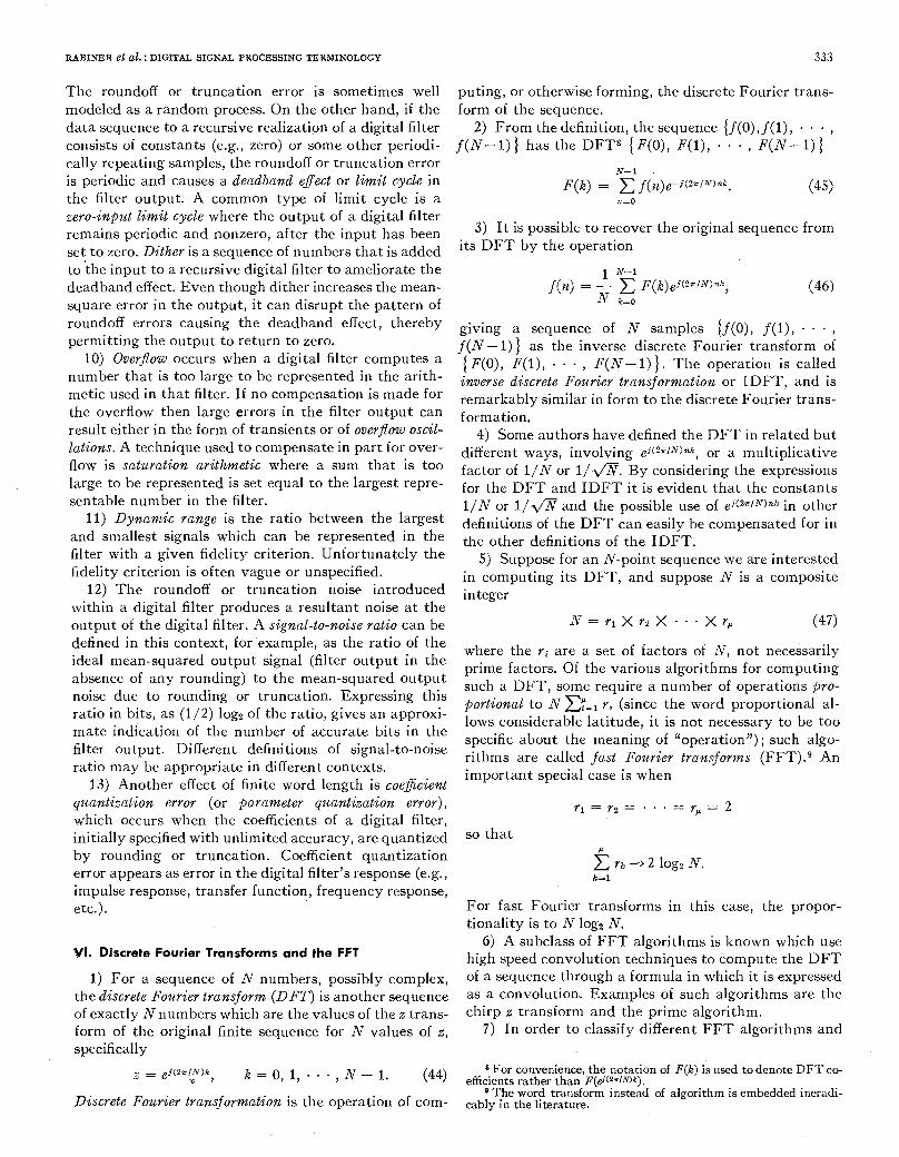
The roundoff or truncation error is sometimes well puting, or otherwise forming, the discrete Fourier trans- modeled as a random process. On the other hand, if the form of the sequence. data sequence to a recursive realization of a digital filter 2) From the definition, the sequence { f ( O ) , f ( l ) , . . . , consists of constants (e.g., zero) or some other periodi- f ( N - 1 ) 1 has the DFT* f F(O) , F(1) , . . , F ( N - 1) 1 cally repeating samples, the roundoff or truncation error is periodic and causes a deadband efect or limit cycle in ~ ( h ) = j (n)e- i (2~/~7)nk. the filter output. A common type of limit cycle is a n-0

zero-input limit cycle where the output of a digital filter

set to zero. Dither is a sequence of numbers that is added its DFT by the ‘peration to ’the input to a recursive digital filter to ameliorate the 1 N-1

deadband effect. Even though dither increases the mean- j(n> = - F ( ~ ) ~ ~ ( z T / N I ” ~ (46) square error in the output, it can disrupt the pattern of roundoff errors causing the deadband effect, thereby giving a sequence of N samples ( f ( o > , f(l) , . . . , permitting the output to return to zero. f ( N - 1) 1 as the inverse discrete Fourier transform of

number that is too large to be represented in the arith- inverse discrete ~~~~i~~ transformation or IDFT, and is metic used in that filter. If no compensation is made for remarkably similar in form to the discrete ~~~~i~~ trans- the overflow then large errors in the filter output can formation. result either in the form of transients or of overjiow oscil- 4) some authors have defined the DFT in related but lations. A technique used to compensate in part for over- different ways, involving e i ( ~ T / ~ ) n k , or a multiplicative flow is saturation arithmetic where a sum tha t is too factor of 1 / ~ or 1/dr. B,, considering the expressions

sentable number in the filter. 1/N or l /dx and the possible use of ei(2T/N)nk in other

and smallest signals which can be represented in the the other definitions of the IDFT. filter with a given fidelity criterion. Unfortunately the 5) suppose for an ~ - ~ ~ i ~ ~ sequence we are interested fidelity criterion is often vague or unspecified. in computing its DFT, and suppose N is a composite

within a digital filter produces a resultant noise a t the output of the digital filter. A signal-to-noise ratio can be A 7 = T I X r2 X . . . X r, (47) defined in this context, for example, as the ratio of the ideal mean-squared output signal (filter output in the

where the r; are a set of factors of N , not necessarily

absence of any rounding) to the mean-squared output prime factors. Of the various algorithms for computing

noise due to rounding or truncation. Expressing this such a DFT, some require a number of operations pro-

ratio in bits, as (1/2) log3 of the ratio, gives an approxi- portional to NE‘, rl (since the word proportional al-

mate indication of the number of accurate bits in the lows considerable latitude, it is not necessary to be too

filter output. Different definitions of signal-to-noise specific about the meaning of “operation”); such algo-

ratio may be appropriate in different contexts. rithms are called fast Fourier transforms (FFT).g An

13) Another effect of finite word length is coeficient important special case is when

quantization error (or parameter quantization error), y l = y z = . . .

which occurs when the coefficients of a digital filter, = r , = 2

initially specified with unlimited accuracy, are quantized SO that by rounding or truncation. Coefficient quantization error appears as error in the digital filter’s response (e.g., impulse response, transfer function, frequency response, etc.). For fast Fourier transforms in this case, the propor-

N- 1

(45)

remains periodic and nonzero, after the input has been 3, I t Possible to recover the original sequence from

N k=o

10) Overjiow occurs when a digital filter computes a { F ( O ) , F O ) , * . ‘ , F(N- 1) 1. The operation is called

large to be represented is set equal to the largest repre- for the DFT and IDFT i t is evident that the constants

11) Dynamic range is the ratio between the largest definitions of the DFT can easily be compensated for in

12) The roundoff or truncation noise introduced integer

P

rk 2 log2 N . k-1

tionality is to N logz N.

VI. Discrete Fourier Transforms and the FFT

1) For a sequence of N numbers, possibly complex, the discrete Fourier transform ( D F T ) is another sequence of exactly N numbers which are the values of the z transform of the original finite sequence for N values of z , specifically

= , 9 ( 2 a / N ) k ~ , K = 0, 1, . * . , N - 1. (44)

Discrete Fourier transformation is the operation of com-

6 ) A subclass of FFT algorithms is known which use high speed convolution techniques to compute the DFT of a sequence through a formula in which i t is expressed as a convolution. Examples of such algorithms are the chirp z transform and the prime algorithm.

7) In order to classify different FFT algorithms and

efficients rather than F(ei@.’N)k).

cably in the literature.

For convenience, the notation of F(k) is used to denote DFT co-

-a The word transform instead of algorithm is embedded ineradi-

334 XEEE TRAKSACTIONS ON AUDIO AND ELECTROACOUSTICS, DECEMBER 1972

to relate them to one another it is useful to consider the following procedure applied to a sequence f (n) of length N where N has a factorization Px Qx R. The reader should generalize to more complicated factorizations. Let us replace the index n by the triplet (no, nl, nz) where

(no, nl, n,) = n = no + Rnl + QR 922 (48)

and 0 5 ?zO < R

O I % l < Q

0 5 n:! < P.

Similarly, we replace the index k by the triplet ( k o , k l , kz) where

(KO, k l , k z ) = k = K O + Pk1 + PQ kz (49)

and O _ < k o < P

O I k l < Q

0 _< k2 < R.

Then (4.5) can be manipulated into the form

Here (PA and (PB are of unit magnitude and have argu- ments dependent on the indices. Equation (SO), if followed as a recipe, suggests a way of computing an N- point DFT as a collection of smaller DFT’s. There are: QR DFT’s of P-point sequences; P R DFT’s of Q-point sequences; and PQ DFT’s of X-point sequences.

The only other operations called for in (SO) are the multiplications by (PA, ( P l j . These have been called twiddle factors, phase fuctors, and rotation factors by various authors.

8) T o save multiplications (SO) is commonly modified in one of two ways. The first \vay is to combine the factors ( P d f and e--i(2T’P)7b2k0 inside the sum over n2 and the factors (PB and e+(zx/Q)nlkl inside the sum over nl. The algorithm so produced has been called a decimation-in- frequency algorithm or a Sande-l‘ukey algorithm.

9) A second way to save multiplications is to combine the factors (PA and e--j(2a!Q)nlkl inside the sum over nl and the factors (PB and e--j(2x/R)f10k2 inside the sum over no. The resulting form of the algorithm is called a Cooley- T u k e y or decimation-in-time algorithm.

10) An algorithm with the twiddle factors explicitly present, as separate multiplications, is neither Cooley- Tukey nor Sande-Tukey.

11) There is a third way to save multiplications, which works only when the factors P , Q, R are relatively prime. By permuting the data sequencef(n) and accept- ing a permuted transform sequence, a formula like (SO)

can be derived in which (PA =(PB = 1. This algorithm is called the prime factor algorithm.

12) Any of the basic forms can be programmed so that each summation is computed and the result stored in the memory formerly occupied by its input data as soon as that input data is no longer needed. In the case of (SO), the amount of extra storage over the N cells needed for the sequence itself is onl~7 the greater of P , Q, or R cells.

A programnled version of an algorithm which takes advantage of this possibility is called in pluce. Unfortu- nately, when storage use is minimized in this way, either the input sequence or the output sequence must be unusually ordered. An example of this unusual order might be that

F(ko + P k l + PQk2) (5 1)

ends up in storage location kz+Rkl+QRko. The unusual ordering may also take place in the use of weights in the algorithm. All such effects are called “digit reversal.” If N is a power of two, and P = Q = R = 2, the effect is called bit reversal.

13) If the factors of N are equal, say to r , the algorithm is called a base-r or radix-r algorithm and, if the factors are different, it is called a mixed-radix algorithm.

14) A common notation is to let W or WA?r represent the reciprocal of the Nth principle root of unity,

Some authors have used

1.5) For the base-2 Cooley-Tukey form of the FFT algorithm, the most fundamental operation is of the form x = A + W’”B

Y = n - 14’”. (53)

The Sande-Tukey form can be obtained by solving for A and B in terms of X and Y,

A = O S ( X + Y) B = 0.5(X - Y)LVJC. (55)

This gives an elementary operation of an inverse transform. The Sande-Tukey form of the forward transform (DFT) is obtained by eliminating the 1/2 and replacing W-k by Wk. From the appearance of the system flow graph for these operations, each operation is called a butterJy.

16) For diagramming the flow of processing data for the FFT, a flow graph notation is used. The flow graph for a trivial eight-point FFT appears as follows:

7

F ( k ) = x f ( n ) W n k , k = 0, 1, . . . , 7 (56) n=O

where

RABINER et al.: DIGITAL SIGNAL PROCESSING TERMIKOLOGY 335

1 \ L 1 2 3 = exp (- j -:).

The flow graph is shown in Fig. 15. 17) Each node represents a variable and the arrows

terminating at that node originate at the nodes whose variables contribute to the value of the variable at that node. The contributions are additive, and the weight of each contribution, if other than unity, is indicated by the constant written close to the arrowhead of the contribution. Each node is assigned a pair of indices n, L. Variables at nodes in row n replace each other as they are computed and are stored in the cell with index n. All nodes in a column L are computed on iteration L. In this form of the algorithm, the exponent of W on the line entering node (n; L) is n.23-L (mod 8). I t can also be seen that for each pair of operands, the second W is W4 = - 1 times the first and that the "butterfly" operation is indeed given by (54).

VII. Discrete Convolution and Spectrum Analysis

1) The Fourier transform (i.e., the z transform evaluated for z = ej2TfT) of a sampled waveform is periodic in frequency, i.e., X(eizrZ"f+fa)) = X(ei2T-Tf ) where f a = 1 / T =sampling frequency. For this reason i t is convenient to represent a negative fyeguency as the equivalent @ m i - tive frequency below the sampling frequency, i.e., f = -fs/20 is equivalent to f = -f,/20+fs=19/20fs. In this manner one need only describe the spectrum in the positive frequency range of 0 5 f < fs. For the DFT this convention also holds. Thus a typical spectrum of a 16-point D F T is shown in Fig. 16. For the above example the number of D F T points was even (16). The first DFT point, X ( 0 ) , corresponds to the Fourier transform evaluated a t 0 frequency. The (N/2+l)st D F T point, X ( N / 2 ) , corresponds to the Fourier transfordevaluated a t half the sampling frequency. The index k corresponds to a frequency f = k / T N in X ( e i Y r T f ) .

2) If the number of points in the D F T were odd, say N = 15, a typical spectrum would be as shown in Fig. 17: In this case there is no D F T point which corresponds to evaluating the Fourier transform at half the sampling frequency.

3 ) The discrete convolution of two sequences can be computed from the inverse discrete Fourier transform of the product of the discrete Fourier transforms of the two sequences. Thus, if X ( k ) and Y ( k ) are the discrete Fourier transforms of x ( n ) and y ( n ) , the inverse discrete Fourier transform of the product of these discrete Fourier transforms produces a periodic discrete convolu- t ion, also called a cyclic or circular discrete convolution or simply a cyclic convolution.

4) The cyclic convolution can be written algebraically as

N- 1 c X((. - 4 ) y ( ( m ) > (58) Wl=O

Fig. 15. The flow graph for an eight-point FFT.

x ( k )

I,

I I I I

I POSITIVE +---I+ NEGATIVE FREQUENCIES N,2 FREQUENCIES N=16

I

Fig. 16. The locations (in frequency) of the DFT points for a 16-point transform.

I X ( k )

0 I FREQUENCIES

POSITIVE +I--+ NEGATIVE FREQUENCIES N=15

Fig. 17. The locations (in frequency) of the DFT points for a 15-point transform.

where ( ( m ) ) means the index is taken modulo N . Equa- tion (58) can be written as

n c X((% - m))y( (m)) + c X((% - m))y((m)>, (59) N- 1

m=O m=n+ 1

or, alternately,

m=O N- 1 + x((m))r((% - m + N ) ) . (60)

WZ=n+l

The simultaneous presence of both summations is generally undesirable for computing ordinary convolutions. For example, if the first summation in (60) is chosen to represent the desired convolution, then the second summation represents an error term. By augmenting both sequences with zeros so that they have the same length N , which is at least as great as one less than the sum of

336 IEEE TRAKSACTIONS ON AUDIO AND ELECTROACOUSTICS, DECEMBEK 1972

the lengths of the two sequences, cyclic convolution can be made to yield the same result as ordinary convolution.

5) This use of the fast Fourier transform to compute discrete convolutions is sometimes calledfast convolution or FFT convolution. This technique can be easily adapted for computing acyclic (i.e., nonperiodic) correlation functions. In this form, it is called fast correlation or FFT correlation.

6) If one of the two sequences is much shorter than the other, the longer sequence can be sectioned into pieces whose discrete convolutions can be computed separately. These discrete convolutions can be com- bined to produce the discrete convolution of the whole sequence. (Sectioning is used because i t reduces the required amounts of computation and memory.) One of these sectioning techniques (overlap-save or select-save) involves computing the inverse DFT of the product of the DFT’s of a) N samples of the input sequence, and b) the shorter sequence augmented with a sufficient number of zeros so that its sequence contains N samples. (Usually N is at least twice as large as the length of the shorter sequence.) Some of the members of the sequence resulting from the inverse DFT are members of the sequence formed by the desired acyclic (i.e., nonperiodic) convolution. (This number of members equals one more than the number of zeros originally augmenting the shorter sequence.) The longer original sequence is advanced by this number of members. Iterating this process gives the whole convolution. The overlap-add technique for sectioning uses a similar technique but additionally requires adding shifted sequences of partial convolutions.

7) A window is a finite sequence, each element of which multiplies a corresponding element of the main sequence. (This is called windowing.) The sequence of products formed by this element-by-element multiplication is often more useful than the main sequence. The Fourier transform of a typical window (sometimes called the spectral window) consists of a mainlobe, which usually contains a large percentage of the energy in the window, and sidelobes which contain the remaining energy in the window.

8) Windows can be used in estimating power spectra. In the direct method, the power spectrum is estimated by computing the square of the absolute value of the DFT of the windowed sequence. The DFT of the windowed sequence is the convolution of the DFT’s of the window and the original sequence. This convolution smoothes the input power spectrum, consequently values of the power spectrum at frequencies separated by less than the width of the rnainlobe of the spectral window can- not be resolved. In addition to this limit on resolution, the estimate of the power spectrum may contain significant leakage, Le., erroneous contributions from components of the power spectrum at frequencies possibly distant from the frequency of interest because of the nonzero energy in the spectral xy-indow sidelohes,

9) Windows are useful in determining the coefficients of a finite impulse response digital filter. In this case, the original sequence consists of samples of the impulse response corresponding to a transfer function which is approximated by the Fourier transform of the sequence of pairwise products; the product sequence is used as the coefficients of the finite impulse response digital filter.

10) Windows are used also in the indirect method of computing a power spectrum. In this method, the sequence consisting of samples of the autocorrelation function is multiplied by the window. The DFT of the resulting sequence is an estimate of the power spectrum.

11) Windows can be used also in estimating cross spectra where the estimates are obtained by multiplying the products of the DFT’s of two or more distinct sequences.

12) The determination of a finite impulse response described by an ordinary convolution is called deconvolution or FIR identification.

Acknowledgment

The authors would like to acknowledge the comments and criticisms of this paper provided by G. D. Bergland, C. H. Coker, D. L. Favin, B. Gold, 0. Hermann, S. Lerman, A. V. Oppenheim, H. 0. Pollak, and H. F. Silverman.

Alphabetic Index of Terms

A A/D Conversion Noise: V-2 Aliasing: 111-4 Amplitude Response: 11-9 Analog: 1-2 Analog Signals: 1-2

Analog Waveforms: 1-2 Analog-to-Digital Converter: V - Z

Analytical Design Technique: IV-32

B Base: V-4 Base R: VI-13 Bilinear Transformation: IV-31 Binary Representation: V-4 Bit Reversal: VI-12 Block-Diagram: 11-11

Butterfly: VI-15 Block Floating-point h:umbers: V-5

Rutterworth Filter: TV-27

C Canonic Form: IV-17 Cascade Canonic Form: IV-17

Causality: IV-21 Causal: IV-22

Chebyshev Filters: 1V-27 Coefficient Quantization Error: V-13 Comb Filter: IV-11 Continuous Time: 1-3 Cooley-Tukey : VI-9 Cyclic or Circular Discrete Conyolutigrl: V I 1 4

D DC Point: 111-2 Deadband Effect: V-9 Dgrimationvin-Frequency: VI-8

RABINER et d.: DIGITAL SIGNAL PROCESSING TERMINOLOGY 337

Decimation-in-Time: VI-9 Deconvolution: VII-12 Digital: 1-5 Digital Aliasing: 111-5 Digital Filter: IV-1 Digital Filter Realizations: IV-17 Digital ImDulse: 11-5

o------ - -

Digital Siinal: 1-5 Digital Simulation: 1-6 Digital System: 1-5 Digital-to-Analog (D/A) Converter: V-1 Digital Waveform: 1-5 Direct Form 1: 1V-17 Direct Form 2: 1V-17 Direct Method: VII-8 Discrete Convolution: VII-3 Discrete Filters: IV-1 Iliscrete Fourier Transform (DFT): V I - 1

Discrete Time: 1-4, 1-5 Iliscrete Fourier Transformation: Vi-1

Discrete-Time Convolution: 11-8 Discrete-Time Impulse: 11-5 Discrete-Time Impulse a t k = k o : 11-5 Discrete-Time Linear Filter: 11-7 Tliscrete-Time Linear System: 11-7 Dither: V-9 Dynamic Range: V-1 1

E Elliptic (Cauer) Filter: IV-27 Equiripple (Optimal) Filter: IV-14 Exponent: V-4 Extraripple Filter: IV-13

F Fast Convolution: VII-5 Fast Correlation: V I I J Fast Fourier Transform (FFT) : V I 4

FFT Correlation: VII-5 FFT Convolution: VI14

Filter Bandwidth: IV-25 Finite Impulse Response (FIR): IV-6 F I R Identification: VII-12 First-Order Section: IV-17 Fixed-point Number: V-3 Floating-point &'umber: V-4 Flow Graph: VI-16 Folding Frequency: 111-3 Fourier Transform: 111-2

Frequency Samples: IV-12 Frequency Response: 11-9

Frequency-Sampling Filter: IV-12 Frequency-Sampling Realization: IV-15 Frequency-Scale Factor: IV-24

G Gain of a Discrete Filter: IV-23 Guard Filter: IV-31

H Hexadecimal Representation: V-4

1 Impulse: 11-5 Impulse Invariance: IV-31

In-Band Ripple: IV-30 Impulse Response: 11-5

Indirect Method: VII-10 Infinite Impulse Response (IIR): IV-7 In-Place: VI-12

Inverse Discrete Fourier 'Transformation (IDFT): VI-3

Inverse z Transform: 11-3 Iterative Optimization Technique: IV-32

K Kalman Filter (Discrete Time): IV-16

L Leakage: VII-8 Limit Cycle: V-9

M Mainlobe: VII-7 Mantissa: V-4 Matched z Transform: IV-31 Minimum Stopband Attenuation: IV-30 Mixed Radix: VI-13 Multiplexed Filter: IV-3 Multirate System: 1-10

N Negative Frequency: VII-1 Next-State Simulation: 1-7 Noise: 1-5 Nonrecursive Filter: IV-5 Nth-Order Systems: 11-10 Nyquist Frequency: 111-3 Nyquist Interval: 111-3 Nyquist Rate: 111-3

0 Object System: 1-6 Octal Representation: V-4 Ones Complement: V-6 One-sided z Transform: 11-1, 11-2 Optimization Technique: IV-32 Ordering: IV-20

Overflow: V-10 Out-of-Band Ripple: IV-30

Overflow Oscillations: V-10 Overlap-Add: VII-6 Overlap-Save: VI 1-6

P

Parallel Canonic Form: IV-17 Pairing: IV-20

Parameter Quantization Error: V-13 Passband Ripple: IV-29 Periodic Discrete Convolution: VII-3 Phase Factors: VI-7

Positive Frequency: VII-1 Phase Response: 11-9

Postfilter: V-1 Prime Factor Algorithm: VI-11 Principle Root of Unity: VI-14

Q Quantizing: V-2 Quantizing Noise: V-2

R Radix R: VI-13 Real-Time Process: 1-8 Reconstruction Device: V-1 Reconstruction Filter: V-1 Recursive Filter: IV-4 Recursive Realization: 11-10

Resolution: VII-8 Resolved : VI 1-8 Ripple: IV-29 Rotation Factors: VI-7 Rounding: V-8 Roundoff Error: V-9 Roundoff Noise: V-9

5 Sample Value: 11-6 Sampled Data: 1-4 Sampled-Data Filter: IV-1 Sampling Frequency: 111-3 Sampling Interval : 1 11-3 Sampling Rate: 1 11-3 Sande-Tukey: VI-8 Saturation Arithmetic: V-10 Second-Order Section: IV-17 Sectioned: VII-6 Sectioning: VII-6 Select-Save: VII-6 Sequences: 1-4

Sidelobes: VII-7 Series Form: IV-17

Sign and Magnitude: V-6 Signal: 1-5 Signal-to-Noise Ratio: V-

Spectral Window: VII-7 Source System: 1-6

Stability: IV-21 Stopband Ripple: IV-30 Switched Filter: IV-2 System Function: 11-9

12

T

Throughput Rate: 1-9 Tapped Delay Line: IV-10

Transition Band: IV-28 Throughput Rate per Signal: 1-9

Transpose Configurations: IV-19 Transition Ratio: IV-28

Transversal Filter: IV-10 Truncation: V-8 Truncation Error: V-9 Truncation Noise: V-9 Twiddle Factors: VI-7 Twos Complement: V-6 Two-sided z Transform: 11-2

U IJndersamnled : 1 11-4 Unit Advcnce: 11-1 Unit Circle: 111-2 Unit Delay Operator: 11-1 Unit Pulse: 11-5

.

Unit Sample: 11-5 Unit Sample Response: 11-5

W Waveform: 1-5 Wiener Filter: IV-16 Window: VII-7 Windowing: VII-7

1

2; Plane: 11-4 z-1 Plane: 11-4 z Transform: 11-1 Zero-Input Limit Cycle: V-9

Documents

Terminology in Digital Signal Processin - UC Santa … in Digital Signal Processin LAWRENCE R. RABINER, JAMES W. COOLEY, HOWARD D. HELMS, LELAND B. JACKSON, JAMES F ... In digital