Embed Size (px)
Citation preview
Test Vehicle for Regenerative Braking
Emulation
Master‟s Thesis in the Master‟s program Automotive Engineering
HORACE LAI AND DAVID MADÅS
Department of Applied Mechanics
Division of Vehicle Engineering and Autonomous Systems
CHALMERS UNIVERSITY OF TECHNOLOGY
Göteborg, Sweden 2011
Master‟s Thesis 2011:10
TM

MASTER‟S THESIS 2011:10
Test Vehicle for Regenerative Braking
Emulation
Master‟s Thesis in the Master‟s Program Automotive Engineering
Horace Lai and David Madås
Department of Applied Mechanics
Division of Vehicle Engineering and Autonomous Systems
CHALMERS UNIVERSITY OF TECHNOLOGY
Göteborg, Sweden 2011
Test Vehicle for Regenerative Braking Emulation
Master‟s Thesis in the Master‟s Program Automotive Engineering
HORACE LAI AND DAVID MADÅS
©Horace Lai and David Madås, 2011
Master‟s Thesis 2011:10
ISSN 1652-8557
Department of Applied Mechanics
Division of Vehicle Engineering and Autonomous Systems
Chalmers University of Technology
SE-412 96 Göteborg
Sweden
Telephone: + 46 (0)31-772 1000
Cover:
Test vehicle during calibration of torque measurement wheels.
Reproservice / Department of Applied Mechanics
Göteborg, Sweden 2011
I
Test Vehicle for Regenerative Braking Emulation
Master‟s Thesis in the Master‟s Program Automotive Engineering
Horace Lai and David Madås
Department of Applied Mechanics
Division of Vehicle Engineering and Autonomous Systems
Chalmers University of Technology
ABSTRACT
The recent increase in global environmental concern drives the development of fuel
saving vehicle technologies. A way to save fuel is to recuperate kinetic energy into a
usable form for propulsive purposes, which is known as regenerative (regen) braking.
However, regen braking also influences the vehicle stability and the driver‟s
perception of the brake system. The impact of the human factor imposes the use of a
test vehicle during development of regen braking strategies. The production of a regen
braking test vehicle was initiated by SAAB as part of their Hybrid Vehicles and
eAWD project and conducted by this master thesis.
The main use of the test vehicle is to analyze the limitations of additive regen braking,
where additional electric motor brake torque is applied on top of the standard brake
torque. Additive braking allows the original brake system to be retained, saving
production costs while giving fuel consumption improvements. Also, it facilitates the
transition process to hybrid vehicles.
The perfect test vehicle for regen braking would possess one electric motor for each
wheel and the necessary ancillaries. However, this vehicle project would have an
intrinsic high level of packaging complexity, cost and engineering time. To overcome
these negative aspects, another concept was conceived, in which a second hydraulic
brake system is controlled to emulate electric motors. Electric motors are emulated in
the sense that the friction brake wheel torque is equal to that produced by an electric
motor. This concept consists of extra calipers clamping the original rotors, an Electro-
Hydraulic Brake (EHB) unit delivering brake pressure and a dSpace onboard
computer running the test program.
Simulink models of a generic electric driveline were developed to emulate the
behavior of regen braking. The models include the battery, electric motor, power
converter, and motor controller. These models calculate the wheel torque to be
applied, which needs to be converted to a pressure value for the EHB unit. A brake
model was developed to calculate the pressure, taking into account the temperature
which affects the friction coefficient between the pad and disc.
A hardware-in-the-loop rig was used for calibration of the brake model. Additionally,
torque measuring wheels were installed on the test vehicle to calibrate the software
and to validate the performance of the vehicle.
The result of this thesis is an easy-to-use test vehicle which can conduct experiments
dealing with additive regen braking, as well as any brake based vehicle system. For
engineers to get started quickly, an example case study and a user manual are
provided. The result of the research utilizing the test vehicle will be seen in the next
generation SAAB hybrid vehicles.
Key words: Regenerative braking, test vehicle, electric vehicles, brake system.

CHALMERS, Applied Mechanics, Master‟s Thesis 2011:10 II
CHALMERS, Applied Mechanics, Master‟s Thesis 2011:10 III
Contents
1 INTRODUCTION 1
1.1 Background 1
1.2 Problem definition 1
1.3 Objectives 1
1.4 Delimitations of work 2
2 USE CASES 3
2.1 Limitations of additive regen braking 3
2.2 Influence of regen braking on handling and stability 4
2.3 Friction and regen brake transitions 5
2.4 Coast regen braking 5
2.5 Other applications 6
3 ELECTRIC VEHICLE SUBSYSTEMS 7
3.1 Friction brakes 7
3.2 Electric machines 9
3.3 Batteries 14
3.4 Power controller (Inverter) 15
4 REGENERATIVE BRAKING EMULATION MODELING 19
4.1 Control system architecture 19
4.2 Overview of modeled subsystems 20
4.3 Brake disc system 21
4.4 Brake demand 25
4.5 Motor controller 25
4.6 Electric motor 28
4.7 Battery 30
4.8 Drivetrain layouts 30
4.9 Vehicle propulsion torque 33
4.10 Economy 34
5 HARDWARE LAYOUT OF THE TEST VEHICLE 35
5.1 Overview 35
5.2 System safety analysis 36
5.3 EHB system 37
CHALMERS, Applied Mechanics, Master‟s Thesis 2011:10 IV
5.4 Steering knuckles & brakes 40
5.5 Signals and sensors 41
6 CALIBRATION AND VALIDATION OF TEST VEHICLE 47
6.1 Software debugging 47
6.2 Test equipment 48
6.3 Calibrated parameters and method 50
6.4 Validation of test vehicle performance 56
6.5 Notes from test driving 65
7 EXAMPLE USE CASE 67
8 CONCLUSIONS 71
9 FUTURE WORK 73
10 REFERENCES 75
CHALMERS, Applied Mechanics, Master‟s Thesis 2011:10 V
Preface
In this thesis, a test vehicle for emulation of regenerative braking has been developed
and tested. The work was carried out from mid September 2010 to early April 2011.
The development of the test vehicle was initiated by SAAB Automobile as part of
their Hybrid Vehicles and eAWD project. Although most of the work was done at
SAAB Automobile, some tests were carried out at Chalmers University of
Technology at the Department of Electrical Engineering. The collaboration with
Chalmers University of Technology also extends to plans of building a similar test
vehicle for use at Chalmers.
Supervisors of the project have been Gunnar Olsson at SAAB Automobile and Peter
Stavered at eAAM. Examiner is Mathias Lidberg at the Department of Applied
Mechanics, Division of Vehicle Engineering and Autonomous Systems at Chalmers
University of Technology. The authors would like to thank Gunnar Olsson, Peter
Stavered and Mathias Lidberg for their invaluable guidance throughout the project as
well as Klas Olsson and Carl Sandberg for their efforts on the Chalmers HIL-rig. The
help from all consulted engineers and workshop workers at SAAB Automobile is
highly appreciated, especially the great efforts of Kjell Carlsson, Klas-Göran Ryrlén
and Jouko Kähkönen.
Trollhättan April 2011
Horace Lai and David Madås
CHALMERS, Applied Mechanics, Master‟s Thesis 2011:10 VI
Notations
Roman upper case letters
𝐴 Area
𝐵 Magnetic flux density
𝐸 Induced electric motor force voltage (e.m.f)
𝐹 Force
𝐼 Electric current
𝑄 Heat
𝑅 Electrical resistance
𝑇 Torque
∆𝑇 Temperature difference
𝑉 Voltage
Roman lower case letters
𝑐 Specific heat
Convection coefficient
𝑘 Thermal conductivity
𝑘𝑒 E.m.f constant
𝑘𝑡 Torque constant
𝑙 Length
𝑚 Mass
𝜇 Friction
𝑛 Number of caliper pistons
𝜔 Rotational velocity
𝑝 pressure
𝑟 Radius
𝑣 Velocity


CHALMERS, Applied Mechanics, Master‟s Thesis 2011:10 1
1 Introduction
1.1 Background
The recent increase in global environmental concern drives the development of fuel
saving vehicle technologies. A way to save fuel is to recuperate kinetic energy into a
usable form for propulsion, which is known as regenerative (regen) braking. There are
substantial amounts of energy to be saved by using regen braking systems, even
though it varies with the vehicle type and driving situation (Wicks and Donnelly).
However, regen braking also influences the vehicle stability and the driver‟s
perception of the brake system. The impact of the human factor necessitates the use of
a test vehicle during development of regen braking strategies. The production of a
regen braking test vehicle was therefore initiated by SAAB as part of their Hybrid
Vehicles and eAWD project and conducted by this master thesis.
1.2 Problem definition
A way of recuperating brake energy is to use an electric motor in generator mode,
providing brake torque while charging a battery. An electric machine is usually unable
to replicate the functionality of friction brakes, as the wheel torque capability is
generally less than for friction brakes. Therefore, a second friction based brake system
should be retained. Mixing friction braking and regen braking is challenging, since the
maximum brake torque of an electric machine varies with vehicle speed. Additionally,
regen braking might influence the stability of the vehicle. These factors imply that a
control strategy should be developed in order to achieve consistent and predictable
vehicle behavior during braking (von Albrichsfeld and Karner) (Hancock and
Assadian).
The ideal test vehicle for regen braking would possess one electric motor for each
wheel, a variety of battery options, a power controller and the necessary ancillaries.
However, such a vehicle project would have an intrinsic high level of packaging
complexity, cost and time. To overcome these negative aspects, another concept was
conceived, in which a hydraulic friction brake system is controlled to emulate electric
motors.
1.3 Objectives
The objective of the Master Thesis is to design and develop a test vehicle with an
Electro-Hydraulic Brake (EHB) system capable of emulating a regen braking system.
The regen system is emulated in the sense that the friction brake wheel torque is equal
to that produced by an electric machine.
The main use of the test vehicle is to analyze the limitations of additive regen braking,
where additional electric motor brake torque is applied on top of the torque of the
original (OEM) brake system. Additive regen braking allows the original brake
system to be retained, saving production costs while giving fuel consumption
improvements. Also, it facilitates the transition process to hybrid vehicles. The
alternative to additive braking is brake blending, which smoothly changes the
proportion of friction brake and regen torque. It requires the implementation of a
brake-by-wire system in the production car. Since the test vehicle is primarily used for
CHALMERS, Applied Mechanics, Master‟s Thesis 2011:10 2
development of additive regen braking, the original brake system is kept untouched.
The test vehicle is then equipped with two brake systems; the OEM system and the
EHB system.
The test vehicle should include software with the necessary vehicle subsystem models
to translate requested wheel torque to required brake pressure output of the EHB.
Generic models of electric driveline components such as electric motors, battery and
power electronics should be developed to emulate an electric vehicle. Also, the
software should have a modular architecture to aid development of new control
models.
A use case analysis should to be conducted. The functionality of the proposed test
vehicle might be useful for the development of other brake-based vehicle control
functions, such as autonomous braking. Possible uses of the vehicle should be
analyzed and their functional requirements taken into consideration when specifying
the test vehicle.
A system safety analysis should be made to identify possible hazards and to
implement the necessary features to handle these. A by-product of the safety analysis
is a user guide booklet, giving instructions on precautions to take and procedures to
use.
Testing is carried out to calibrate the software and evaluate the performance of the
installed system. For calibration of the brake disc heat model, Hardware-In-the-Loop
(HIL) testing is carried out. The function of the test vehicle is validated by measuring
the precision and the response of the brake application.
1.4 Delimitations of work
All mechanical work is done by the Saab prototype and chassis workshops. All
modeling work is done in Matlab/Simulink (not in lower level programming language
such as C).
CHALMERS, Applied Mechanics, Master‟s Thesis 2011:10 3
2 Use Cases
The possible use cases for the test vehicle are described to make sure it has the
required functionality. The compilation of use cases was done with help from chassis
& powertrain controls engineers from SAAB (Olsson, Klomp and Eklund). For all use
cases, important software functions, performance requirements and required signals
and sensors are identified.
2.1 Limitations of additive regen braking
The maximum brake torque of an electric motor varies with vehicle speed. Therefore,
to produce constant deceleration for a constant brake demand for all vehicle
velocities, the braking effort has to be smoothly blended between the electric motor
and the friction brakes (von Albrichsfeld and Karner). The implementation of a brake-
by-wire (BBW) system is a costly procedure. Also, it posts a number of new, mostly
safety related, challenges (Hoseinnezhad and Bab-Hadiashar). An interesting topic is
whether it is feasible to retain the standard mechanical-hydraulic brake system with
added regen braking. This is called additive regen braking.
The pedal feel could be said to be the driver‟s perception of the correlation between
the pedal input and the realized vehicle deceleration. Characteristics of the pedal feel
include the brake controllability, progressiveness, effort and sponginess (de Arruda
Pereira) (Rajesh, Badal and Pol). The pedal feel gives feedback on brake performance
(Day, Ho and Hussain), influences the perceived quality of the brake system and is
important for the driver‟s confidence in the system (Pascali, Ricci and Caviasso). As
the amount of additive regen increases, the regulation required and the effects of
electric driveline failure increases as well. The problem is to determine how much
additive regen braking can be done before the driver perceives the additive braking as
unpredictable and unsafe.
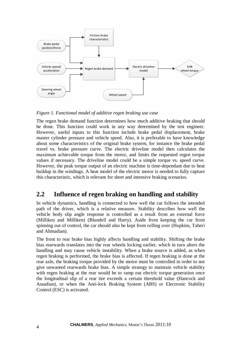
Figure 1 displays a suggested functional model for this use case. This can be said to
be the flow of information through the control system of the test vehicle. The starting
point is the input parameters, which are then used by function blocks, representing a
strategy or a modeled subsystem. The output is the requested EHB brake torque
values at the wheel of all four corners of the car.
CHALMERS, Applied Mechanics, Master‟s Thesis 2011:10 4
Regen brake demandElectric driveline
model
Wheel speed
Brake pedal position/force
Vehicle speed/acceleration
EHB wheel torque
Friction brake characteristics
Steering wheel angle
Figure 1. Functional model of additive regen braking use case
The regen brake demand function determines how much additive braking that should
be done. This function could work in any way determined by the test engineer.
However, useful inputs to this function include brake pedal displacement, brake
master cylinder pressure and vehicle speed. Also, it is preferable to have knowledge
about some characteristics of the original brake system, for instance the brake pedal
travel vs. brake pressure curve. The electric driveline model then calculates the
maximum achievable torque from the motor, and limits the requested regen torque
values if necessary. The driveline model could be a simple torque vs. speed curve.
However, the peak torque output of an electric machine is time-dependant due to heat
buildup in the windings. A heat model of the electric motor is needed to fully capture
this characteristic, which is relevant for short and intensive braking scenarios.
2.2 Influence of regen braking on handling and stability
In vehicle dynamics, handling is connected to how well the car follows the intended
path of the driver, which is a relative measure. Stability describes how well the
vehicle body slip angle response is controlled as a result from an external force
(Milliken and Milliken) (Blundell and Harty). Aside from keeping the car from
spinning out of control, the car should also be kept from rolling over (Hopkins, Taheri
and Ahmadian).
The front to rear brake bias highly affects handling and stability. Shifting the brake
bias rearwards translates into the rear wheels locking earlier, which in turn alters the
handling and may cause vehicle instability. When a brake source is added, as when
regen braking is performed, the brake bias is affected. If regen braking is done at the
rear axle, the braking torque provided by the motor must be controlled in order to not
give unwanted rearwards brake bias. A simple strategy to maintain vehicle stability
with regen braking at the rear would be to ramp out electric torque generation once
the longitudinal slip of a rear tire exceeds a certain threshold value (Hancock and
Assadian), or when the Anti-lock Braking System (ABS) or Electronic Stability
Control (ESC) is activated.
CHALMERS, Applied Mechanics, Master‟s Thesis 2011:10 5
A functional model for this use case would be very similar to that in Figure 1.
Interesting parameters to be fed into to the brake demand function include
longitudinal tire slip, vehicle acceleration and yaw rate. Also, the activation of the
ABS and ESC units should be monitored.
Another parameter that would be useful for this use case is the road friction
coefficient. In (Shim and Margolis), great improvements in vehicle stability control
were shown when the road surface friction was known. In (Andersson, Bruzelius and
Callesgren), an implementation of a road friction estimation system was done.
Considering this, the test vehicle should be able to incorporate signals from
instruments used to measure the road friction, for instance force transducers and
optical sensors.
2.3 Friction and regen brake transitions
Braking transitions include every case when the standard friction brakes or the regen
braking are put on or off. Needless to say, the time response and the driver‟s
perception of the change in brake torque are of main interest. At the event of a panic
braking, the regenerative braking is ramped out to zero since it may cause vehicle
instability. It is vital that the friction brake modulator is quick enough to cover the
requested braking effort during the regen ramp out. Otherwise, the driver might sense
the transition as a sudden lack of brakes. If the regen brakes are off completely before
the friction brakes are applied, the driver might even get the feeling of acceleration.
The seriousness of the matter can be exemplified by Toyota, which 2010 was faced
with having to recall their Prius (BBC news). Customers complained about the car
feeling unsecure during braking.
For a brake transition strategy function, the value and rate of change of brake pedal
displacement can be used to recognize panic braking. Other interesting parameters to
observe are wheel slip and vehicle longitudinal acceleration. The brake pressures of
the standard brake system could be used to calculate the buildup of friction brake
force.
2.4 Coast regen braking
Coast regen is the application of regen braking during zero driver braking and throttle
input; during coasting. The amount of regen braking performed is relatively small. It
is possible to compare the scenario as being similar to increasing the amount of
internal combustion engine braking. If the throttle travel goes from point A to point B,
the point of zero engine torque can be moved slightly from point A towards point B.
Letting off the throttle pedal completely would then result in a negative propulsion
torque request. The main interest in the coast regen use case is to evaluate the driver‟s
perception of this increased engine braking. The limit of coast regen is set by what the
driver perceives as comfortable. This use case might be investigated together with the
limitations of additive braking use case. Since the maximum amount of recuperation
is lower for additive regen braking than for a blended braking system, more coast
regen can be implemented to recuperate useful amounts of energy.
An important input for a coast regen strategy function is the throttle pedal
(accelerator) position. Other vehicle states, such as the vehicle speed and engine
torque might be desired.
CHALMERS, Applied Mechanics, Master‟s Thesis 2011:10 6
2.5 Other applications
Essentially, the EHB system of the test vehicle delivers wheel torque according to the
implemented software. This general function may be useful for testing of various
vehicle systems, even those unrelated to regen braking.
The test vehicle can be used for development of active safety systems. This could be
crash mitigation/prevention or avoidance maneuvers. Crash mitigation deals with
sensing a possible hazard and decreasing the severity of the situation by decelerating
the car. Avoidance maneuvers use the brakes to steer the car out of harm‟s way.
Torque vectoring distributes the propulsion torque between the four wheels to aid
maneuverability. In the test vehicle, torque vectoring can be achieved by using the
friction brakes to brake one of the front wheels, while adding propulsive torque to
maintain the vehicle speed. This approach is lighter and cheaper compared to complex
electro-mechanical devices and adds functionality to already existing components.
Many vehicle systems that use the brakes for functionality can be developed using the
test car. The control system of the test vehicle should have interfaces to implement
any required sensory information.
CHALMERS, Applied Mechanics, Master‟s Thesis 2011:10 7
3 Electric Vehicle Subsystems
The basis of the test vehicle‟s EHB control system functions requires knowledge of
friction brakes theory. Also, the regenerative braking application of the vehicle
requires basic theory on electric motors, batteries, and power converters.
3.1 Friction brakes
Equation 3.1 shows the relationship between brake pressure p, caliper piston area A,
brake torque T, the number of pistons 𝑛, the number of brake pads 𝑚, pad/disc
friction coefficient 𝜇, and average pad radius 𝑟. The average pad radius is measured
from the center of the disc to where the total friction force from the pad is applied.
𝑇 = 𝐹𝑟 = 𝑛𝑝𝐴(𝑚𝜇)𝑟
𝑝 =𝑇
𝑚𝑛𝐴𝜇𝑟 Equation 3.1
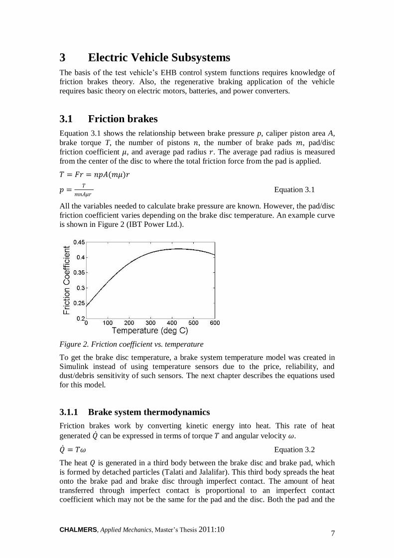
All the variables needed to calculate brake pressure are known. However, the pad/disc
friction coefficient varies depending on the brake disc temperature. An example curve
is shown in Figure 2 (IBT Power Ltd.).
Figure 2. Friction coefficient vs. temperature
To get the brake disc temperature, a brake system temperature model was created in
Simulink instead of using temperature sensors due to the price, reliability, and
dust/debris sensitivity of such sensors. The next chapter describes the equations used
for this model.
3.1.1 Brake system thermodynamics
Friction brakes work by converting kinetic energy into heat. This rate of heat
generated 𝑄 can be expressed in terms of torque 𝑇 and angular velocity 𝜔.
𝑄 = 𝑇𝜔 Equation 3.2
The heat 𝑄 is generated in a third body between the brake disc and brake pad, which
is formed by detached particles (Talati and Jalalifar). This third body spreads the heat
onto the brake pad and brake disc through imperfect contact. The amount of heat
transferred through imperfect contact is proportional to an imperfect contact
coefficient which may not be the same for the pad and the disc. Both the pad and the
CHALMERS, Applied Mechanics, Master‟s Thesis 2011:10 8
disc have masses that absorb the heat energy. The amount of heat energy absorbed is
dictated by the definition of specific heat, Equation 3.3, where 𝑚 is the mass, 𝑐 is the
specific heat, and ∆𝑇 is the difference in temperature between two instances.
𝑄 = 𝑚𝑐∆𝑇 Equation 3.3
Once the heat is transferred to the brake disc and brake pad contact area, it will
conduct into the rest of the brake disc. The thermal conduction behavior is described
by Fourier‟s Law, Equation 3.4, which assumes heat is transferred along an axis with
only one degree of freedom. In this equation, 𝑄 is heat energy, 𝑘 is the thermal
conductivity, 𝐴 is the cross sectional area, 𝑥 is the distance in which the heat has
travelled, and ∆𝑇 is the temperature difference across 𝑥.
𝑄 =𝑘𝐴
𝑥∆𝑇 Equation 3.4
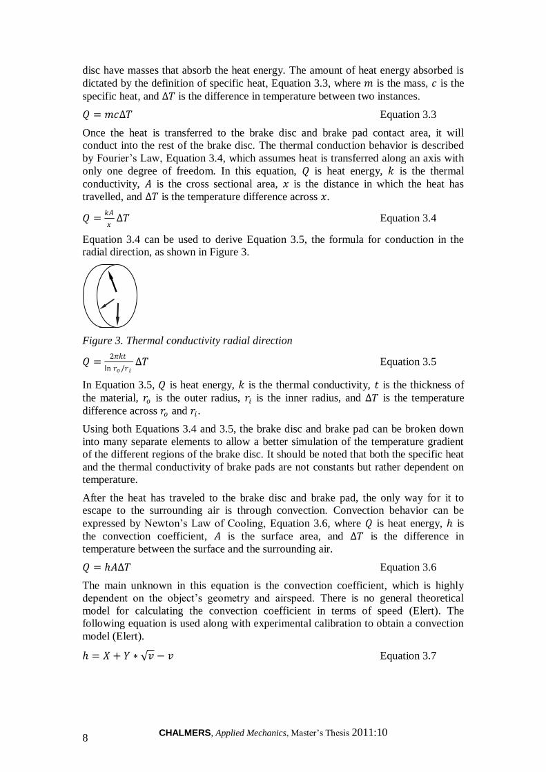
Equation 3.4 can be used to derive Equation 3.5, the formula for conduction in the
radial direction, as shown in Figure 3.
Figure 3. Thermal conductivity radial direction
𝑄 =2𝜋𝑘𝑡
ln 𝑟𝑜/𝑟𝑖 ∆𝑇 Equation 3.5
In Equation 3.5, 𝑄 is heat energy, 𝑘 is the thermal conductivity, 𝑡 is the thickness of
the material, 𝑟𝑜 is the outer radius, 𝑟𝑖 is the inner radius, and ∆𝑇 is the temperature
difference across 𝑟𝑜 and 𝑟𝑖 .
Using both Equations 3.4 and 3.5, the brake disc and brake pad can be broken down
into many separate elements to allow a better simulation of the temperature gradient
of the different regions of the brake disc. It should be noted that both the specific heat
and the thermal conductivity of brake pads are not constants but rather dependent on
temperature.
After the heat has traveled to the brake disc and brake pad, the only way for it to
escape to the surrounding air is through convection. Convection behavior can be
expressed by Newton‟s Law of Cooling, Equation 3.6, where 𝑄 is heat energy, is
the convection coefficient, 𝐴 is the surface area, and ∆𝑇 is the difference in
temperature between the surface and the surrounding air.
𝑄 = 𝐴∆𝑇 Equation 3.6
The main unknown in this equation is the convection coefficient, which is highly
dependent on the object‟s geometry and airspeed. There is no general theoretical
model for calculating the convection coefficient in terms of speed (Elert). The
following equation is used along with experimental calibration to obtain a convection
model (Elert).
= 𝑋 + 𝑌 ∗ 𝑣 − 𝑣 Equation 3.7
CHALMERS, Applied Mechanics, Master‟s Thesis 2011:10 9
Since the brake disc has a very complex geometry, with air vents sandwiched between
two thick iron plates, the convection coefficient may not be the same for all these
surfaces. Dividing the brake disc into various elements helps cope with this challenge.
This is further explained in Chapter 4.3.
3.2 Electric machines
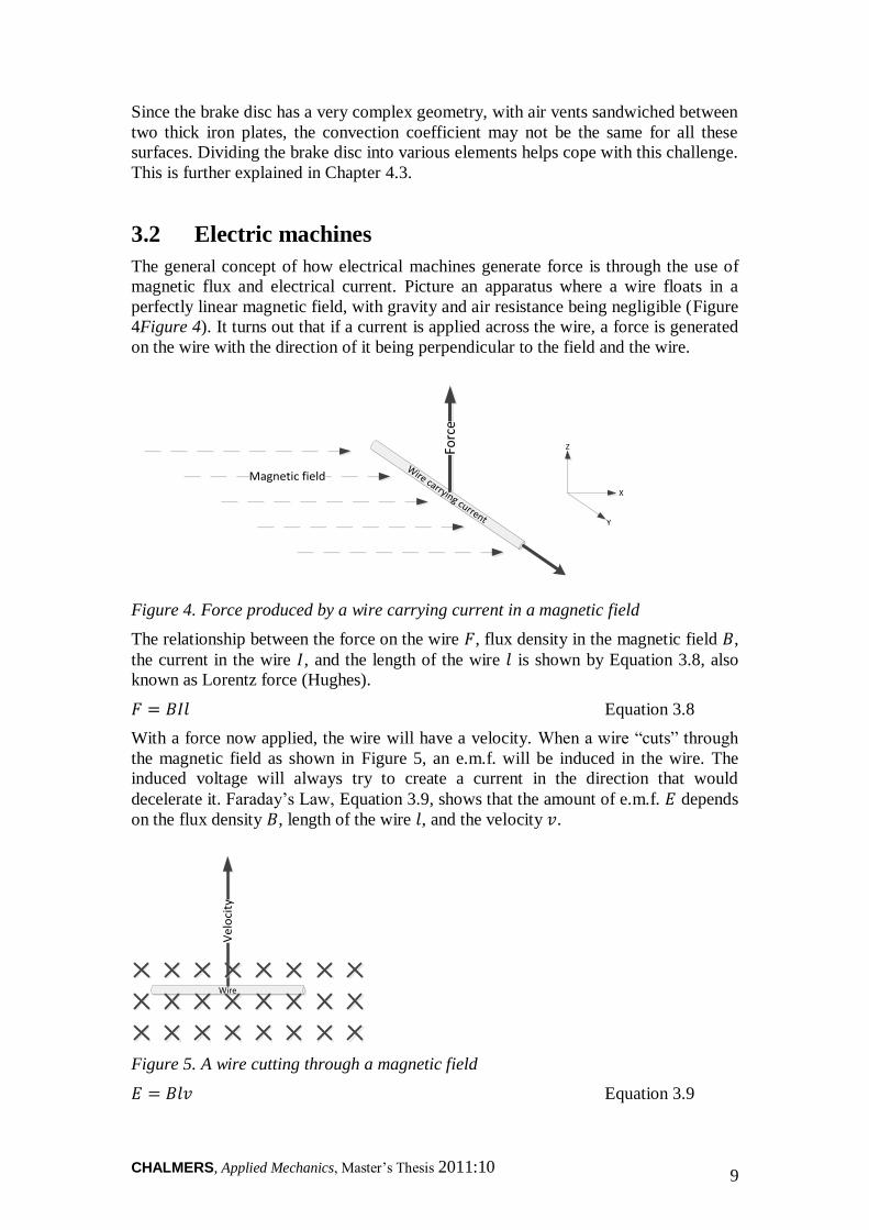
The general concept of how electrical machines generate force is through the use of
magnetic flux and electrical current. Picture an apparatus where a wire floats in a
perfectly linear magnetic field, with gravity and air resistance being negligible (Figure
4Figure 4). It turns out that if a current is applied across the wire, a force is generated
on the wire with the direction of it being perpendicular to the field and the wire.
Magnetic fieldW
ire carrying current
Forc
eZ
Y
X
Figure 4. Force produced by a wire carrying current in a magnetic field
The relationship between the force on the wire 𝐹, flux density in the magnetic field 𝐵,
the current in the wire 𝐼, and the length of the wire 𝑙 is shown by Equation 3.8, also
known as Lorentz force (Hughes).
𝐹 = 𝐵𝐼𝑙 Equation 3.8
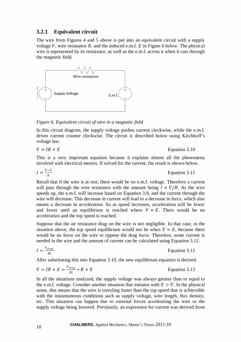
With a force now applied, the wire will have a velocity. When a wire “cuts” through
the magnetic field as shown in Figure 5, an e.m.f. will be induced in the wire. The
induced voltage will always try to create a current in the direction that would
decelerate it. Faraday‟s Law, Equation 3.9, shows that the amount of e.m.f. 𝐸 depends
on the flux density 𝐵, length of the wire 𝑙, and the velocity 𝑣.
Wire
Ve
loci
ty
Figure 5. A wire cutting through a magnetic field
𝐸 = 𝐵𝑙𝑣 Equation 3.9
CHALMERS, Applied Mechanics, Master‟s Thesis 2011:10 10
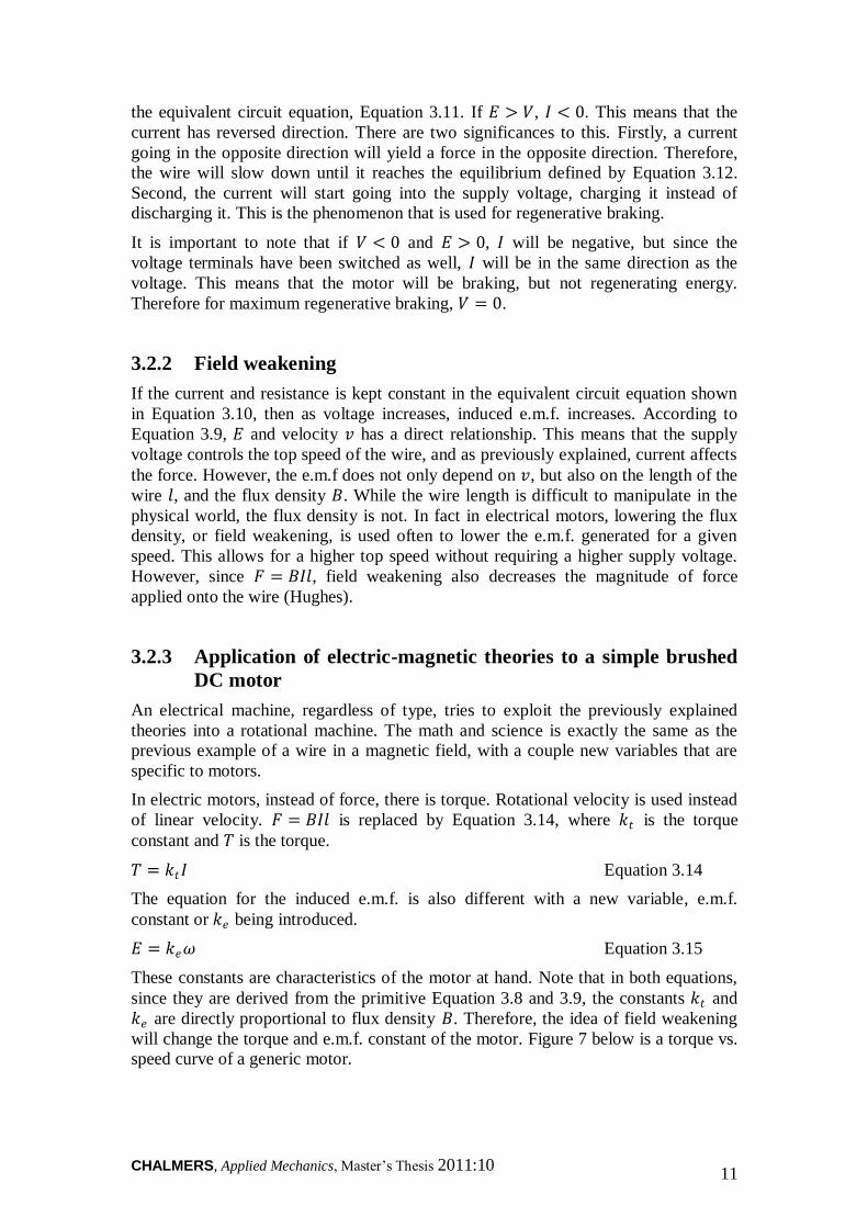
3.2.1 Equivalent circuit
The wire from Figures 4 and 5 above is put into an equivalent circuit with a supply
voltage 𝑉, wire resistance 𝑅, and the induced e.m.f. 𝐸 in Figure 6 below. The physical
wire is represented by its resistance, as well as the e.m.f. across it when it cuts through
the magnetic field.
Wire resistance
Supply Voltage E.m.f.
Figure 6. Equivalent circuit of wire in a magnetic field
In this circuit diagram, the supply voltage pushes current clockwise, while the e.m.f.
drives current counter clockwise. The circuit is described below using Kirchhoff‟s
voltage law.
𝑉 = 𝐼𝑅 + 𝐸 Equation 3.10
This is a very important equation because it explains almost all the phenomena
involved with electrical motors. If solved for the current, the result is shown below.
𝐼 =𝑉−𝐸
𝑅 Equation 3.11
Recall that if the wire is at rest, there would be no e.m.f. voltage. Therefore a current
will pass through the wire resistance with the amount being 𝐼 = 𝑉/𝑅. As the wire
speeds up, the e.m.f. will increase based on Equation 3.9, and the current through the
wire will decrease. This decrease in current will lead to a decrease in force, which also
means a decrease in acceleration. So as speed increases, acceleration will be lower
and lower until an equilibrium is reached where 𝑉 = 𝐸. There would be no
acceleration and the top speed is reached.
Suppose that the air resistance drag on the wire is not negligible. In that case, in the
situation above, the top speed equilibrium would not be when 𝑉 = 𝐸, because there
would be no force on the wire to oppose the drag force. Therefore, some current is
needed in the wire and the amount of current can be calculated using Equation 3.12.
𝐼 =𝐹𝑑𝑟𝑎𝑔
𝐵𝑙 Equation 3.12
After substituting this into Equation 3.10, the new equilibrium equation is derived.
𝑉 = 𝐼𝑅 + 𝐸 =𝐹𝑑𝑟𝑎𝑔
𝐵𝑙∗ 𝑅 + 𝐸 Equation 3.13
In all the situations analyzed, the supply voltage was always greater than or equal to
the e.m.f. voltage. Consider another situation that initiates with 𝐸 > 𝑉. In the physical
sense, this means that the wire is traveling faster than the top speed that is achievable
with the instantaneous conditions such as supply voltage, wire length, flux density,
etc. This situation can happen due to external forces accelerating the wire or the
supply voltage being lowered. Previously, an expression for current was derived from
CHALMERS, Applied Mechanics, Master‟s Thesis 2011:10 11
the equivalent circuit equation, Equation 3.11. If 𝐸 > 𝑉, 𝐼 < 0. This means that the
current has reversed direction. There are two significances to this. Firstly, a current
going in the opposite direction will yield a force in the opposite direction. Therefore,
the wire will slow down until it reaches the equilibrium defined by Equation 3.12.
Second, the current will start going into the supply voltage, charging it instead of
discharging it. This is the phenomenon that is used for regenerative braking.
It is important to note that if 𝑉 < 0 and 𝐸 > 0, 𝐼 will be negative, but since the
voltage terminals have been switched as well, 𝐼 will be in the same direction as the
voltage. This means that the motor will be braking, but not regenerating energy.
Therefore for maximum regenerative braking, 𝑉 = 0.
3.2.2 Field weakening
If the current and resistance is kept constant in the equivalent circuit equation shown
in Equation 3.10, then as voltage increases, induced e.m.f. increases. According to
Equation 3.9, 𝐸 and velocity 𝑣 has a direct relationship. This means that the supply
voltage controls the top speed of the wire, and as previously explained, current affects
the force. However, the e.m.f does not only depend on 𝑣, but also on the length of the
wire 𝑙, and the flux density 𝐵. While the wire length is difficult to manipulate in the
physical world, the flux density is not. In fact in electrical motors, lowering the flux
density, or field weakening, is used often to lower the e.m.f. generated for a given
speed. This allows for a higher top speed without requiring a higher supply voltage.
However, since 𝐹 = 𝐵𝐼𝑙, field weakening also decreases the magnitude of force
applied onto the wire (Hughes).
3.2.3 Application of electric-magnetic theories to a simple brushed
DC motor
An electrical machine, regardless of type, tries to exploit the previously explained
theories into a rotational machine. The math and science is exactly the same as the
previous example of a wire in a magnetic field, with a couple new variables that are
specific to motors.
In electric motors, instead of force, there is torque. Rotational velocity is used instead
of linear velocity. 𝐹 = 𝐵𝐼𝑙 is replaced by Equation 3.14, where 𝑘𝑡 is the torque
constant and 𝑇 is the torque.
𝑇 = 𝑘𝑡𝐼 Equation 3.14
The equation for the induced e.m.f. is also different with a new variable, e.m.f.
constant or 𝑘𝑒 being introduced.
𝐸 = 𝑘𝑒𝜔 Equation 3.15
These constants are characteristics of the motor at hand. Note that in both equations,
since they are derived from the primitive Equation 3.8 and 3.9, the constants 𝑘𝑡 and
𝑘𝑒 are directly proportional to flux density 𝐵. Therefore, the idea of field weakening
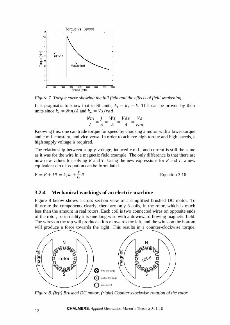
will change the torque and e.m.f. constant of the motor. Figure 7 below is a torque vs.
speed curve of a generic motor.
CHALMERS, Applied Mechanics, Master‟s Thesis 2011:10 12
Figure 7. Torque curve showing the full field and the effects of field weakening
It is pragmatic to know that in SI units, 𝑘𝑡 = 𝑘𝑒 = 𝑘. This can be proven by their
units since 𝑘𝑡 = 𝑁𝑚/𝐴 and 𝑘𝑒 = 𝑉𝑠/𝑟𝑎𝑑.
𝑁𝑚
𝐴=
𝐽
𝐴=
𝑊𝑠
𝐴=
𝑉𝐴𝑠
𝐴=
𝑉𝑠
𝑟𝑎𝑑
Knowing this, one can trade torque for speed by choosing a motor with a lower torque
and e.m.f. constant, and vice versa. In order to achieve high torque and high speeds, a
high supply voltage is required.
The relationship between supply voltage, induced e.m.f., and current is still the same
as it was for the wire in a magnetic field example. The only difference is that there are
now new values for solving 𝐸 and 𝑇. Using the new expressions for 𝐸 and 𝑇, a new
equivalent circuit equation can be formulated.
𝑉 = 𝐸 + 𝐼𝑅 = 𝑘𝑒𝜔 +𝑇
𝑘𝑡𝑅 Equation 3.16
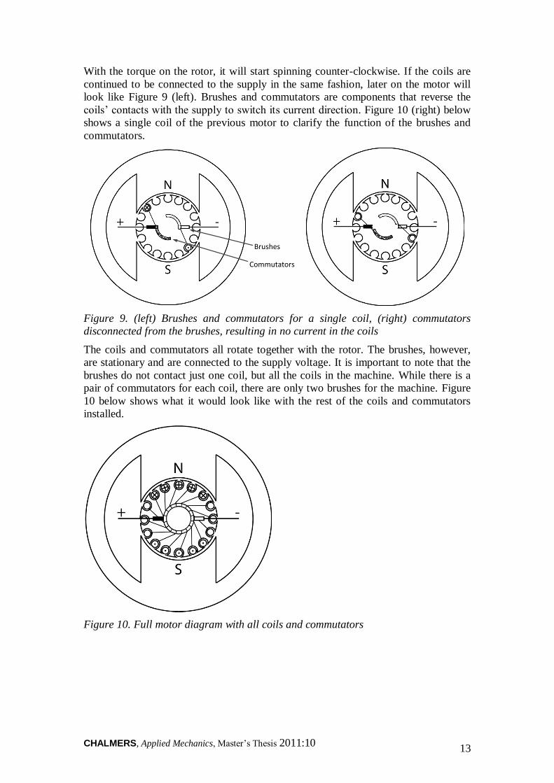
3.2.4 Mechanical workings of an electric machine
Figure 8 below shows a cross section view of a simplified brushed DC motor. To
illustrate the components clearly, there are only 8 coils, in the rotor, which is much
less than the amount in real rotors. Each coil is two connected wires on opposite ends
of the rotor, so in reality it is one long wire with a downward flowing magnetic field.
The wires on the top will produce a force towards the left, and the wires on the bottom
will produce a force towards the right. This results in a counter-clockwise torque.
Figure 8. (left) Brushed DC motor, (right) Counter-clockwise rotation of the rotor
CHALMERS, Applied Mechanics, Master‟s Thesis 2011:10 13
With the torque on the rotor, it will start spinning counter-clockwise. If the coils are
continued to be connected to the supply in the same fashion, later on the motor will
look like Figure 9 (left). Brushes and commutators are components that reverse the
coils‟ contacts with the supply to switch its current direction. Figure 10 (right) below
shows a single coil of the previous motor to clarify the function of the brushes and
commutators.
Brushes
Commutators
Figure 9. (left) Brushes and commutators for a single coil, (right) commutators
disconnected from the brushes, resulting in no current in the coils
The coils and commutators all rotate together with the rotor. The brushes, however,
are stationary and are connected to the supply voltage. It is important to note that the
brushes do not contact just one coil, but all the coils in the machine. While there is a
pair of commutators for each coil, there are only two brushes for the machine. Figure
10 below shows what it would look like with the rest of the coils and commutators
installed.
Figure 10. Full motor diagram with all coils and commutators
CHALMERS, Applied Mechanics, Master‟s Thesis 2011:10 14
3.3 Batteries
Batteries provide current through a cathode and an anode, which is the positive and
negative end of the battery, respectively. By nature, electrons at the anode are
attracted to the cathode. However, an electrolyte in the battery separates these two
ends of the battery, and the electrons have to find another route to the cathode. This is
why, when the battery is connected to a load, current passes through, since it is the
only way for electrons to reach the cathode.
There are various types of batteries used for vehicles. Lead-acid is usually used for
normal car batteries due to their longevity, but are heavy relative to their capacity. For
hybrid vehicles, Lithium-ion batteries are used instead. Some electric race
motorcycles use super capacitors due to their high discharge rates and low weight
despite their low energy capacity. These characteristics of batteries are explained in
more detail below.
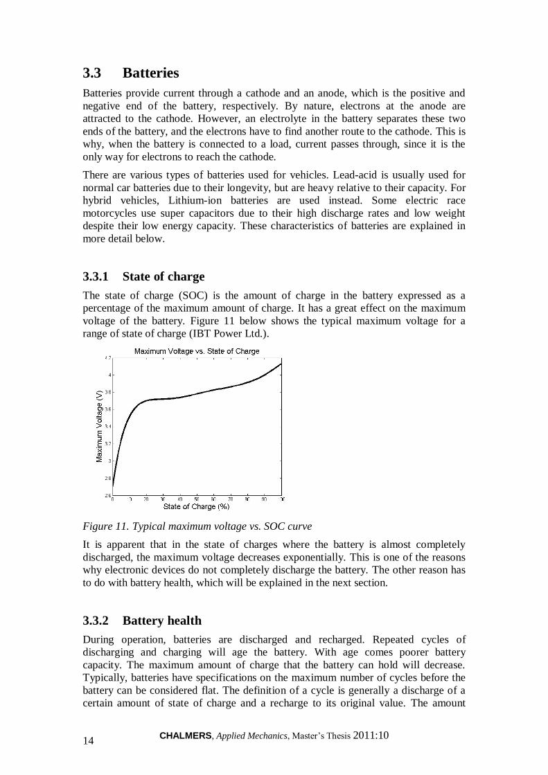
3.3.1 State of charge
The state of charge (SOC) is the amount of charge in the battery expressed as a
percentage of the maximum amount of charge. It has a great effect on the maximum
voltage of the battery. Figure 11 below shows the typical maximum voltage for a
range of state of charge (IBT Power Ltd.).
Figure 11. Typical maximum voltage vs. SOC curve
It is apparent that in the state of charges where the battery is almost completely
discharged, the maximum voltage decreases exponentially. This is one of the reasons
why electronic devices do not completely discharge the battery. The other reason has
to do with battery health, which will be explained in the next section.
3.3.2 Battery health
During operation, batteries are discharged and recharged. Repeated cycles of
discharging and charging will age the battery. With age comes poorer battery
capacity. The maximum amount of charge that the battery can hold will decrease.
Typically, batteries have specifications on the maximum number of cycles before the
battery can be considered flat. The definition of a cycle is generally a discharge of a
certain amount of state of charge and a recharge to its original value. The amount
CHALMERS, Applied Mechanics, Master‟s Thesis 2011:10 15
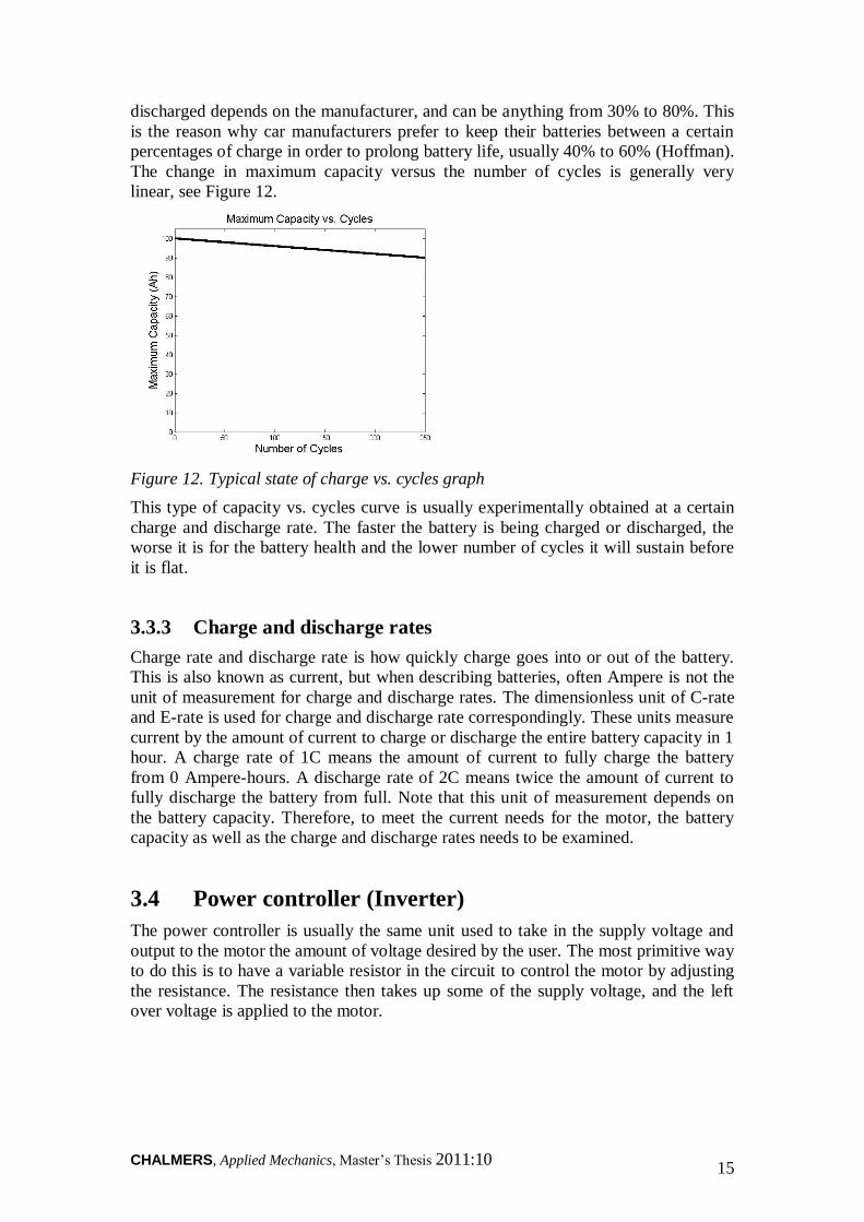
discharged depends on the manufacturer, and can be anything from 30% to 80%. This
is the reason why car manufacturers prefer to keep their batteries between a certain
percentages of charge in order to prolong battery life, usually 40% to 60% (Hoffman).
The change in maximum capacity versus the number of cycles is generally very
linear, see Figure 12.
Figure 12. Typical state of charge vs. cycles graph
This type of capacity vs. cycles curve is usually experimentally obtained at a certain
charge and discharge rate. The faster the battery is being charged or discharged, the
worse it is for the battery health and the lower number of cycles it will sustain before
it is flat.
3.3.3 Charge and discharge rates
Charge rate and discharge rate is how quickly charge goes into or out of the battery.
This is also known as current, but when describing batteries, often Ampere is not the
unit of measurement for charge and discharge rates. The dimensionless unit of C-rate
and E-rate is used for charge and discharge rate correspondingly. These units measure
current by the amount of current to charge or discharge the entire battery capacity in 1
hour. A charge rate of 1C means the amount of current to fully charge the battery
from 0 Ampere-hours. A discharge rate of 2C means twice the amount of current to
fully discharge the battery from full. Note that this unit of measurement depends on
the battery capacity. Therefore, to meet the current needs for the motor, the battery
capacity as well as the charge and discharge rates needs to be examined.
3.4 Power controller (Inverter)
The power controller is usually the same unit used to take in the supply voltage and
output to the motor the amount of voltage desired by the user. The most primitive way
to do this is to have a variable resistor in the circuit to control the motor by adjusting
the resistance. The resistance then takes up some of the supply voltage, and the left
over voltage is applied to the motor.
CHALMERS, Applied Mechanics, Master‟s Thesis 2011:10 16
M
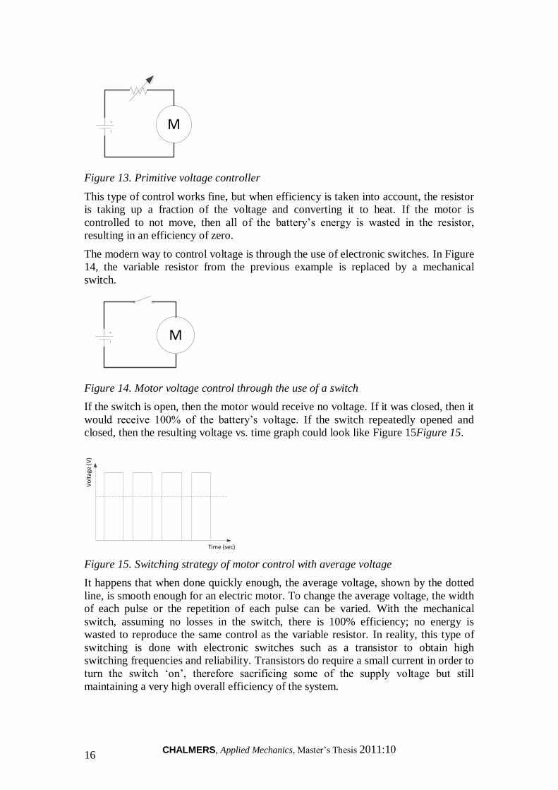
Figure 13. Primitive voltage controller
This type of control works fine, but when efficiency is taken into account, the resistor
is taking up a fraction of the voltage and converting it to heat. If the motor is
controlled to not move, then all of the battery‟s energy is wasted in the resistor,
resulting in an efficiency of zero.
The modern way to control voltage is through the use of electronic switches. In Figure
14, the variable resistor from the previous example is replaced by a mechanical
switch.
M
Figure 14. Motor voltage control through the use of a switch
If the switch is open, then the motor would receive no voltage. If it was closed, then it
would receive 100% of the battery‟s voltage. If the switch repeatedly opened and
closed, then the resulting voltage vs. time graph could look like Figure 15Figure 15.
Time (sec)
Vo
ltag
e (V
)
Figure 15. Switching strategy of motor control with average voltage
It happens that when done quickly enough, the average voltage, shown by the dotted
line, is smooth enough for an electric motor. To change the average voltage, the width
of each pulse or the repetition of each pulse can be varied. With the mechanical
switch, assuming no losses in the switch, there is 100% efficiency; no energy is
wasted to reproduce the same control as the variable resistor. In reality, this type of
switching is done with electronic switches such as a transistor to obtain high
switching frequencies and reliability. Transistors do require a small current in order to
turn the switch „on‟, therefore sacrificing some of the supply voltage but still
maintaining a very high overall efficiency of the system.

CHALMERS, Applied Mechanics, Master‟s Thesis 2011:10 17
It is not very important in this project to model and understand the complexities of the
power converter, since they mostly deal with flexibility and efficiency of the
electronics. In this thesis, the power converter was modeled in a very simple way,
with the power drawn out of the battery being a little higher than the power required
by the motor due to some user defined constant efficiency value. In practice, very
often the motor characteristics are modeled along with the controller and power
converters required to operate the motor.

CHALMERS, Applied Mechanics, Master‟s Thesis 2011:10 18
CHALMERS, Applied Mechanics, Master‟s Thesis 2011:10 19
4 Regenerative Braking Emulation Modeling
For all purposes of the test vehicle, the EHB unit requires CAN messages to be sent
from the software in order to apply pressure to the brakes. Overall, the software
includes sensor data processing functions, the test function and the translation from
requested torque to EHB pressure. To translate torque to pressure, a model of the
brake system is required. For the purpose of regen braking simulation, virtual electric
driveline components are implemented.
4.1 Control system architecture
It is desirable to make the test vehicle software versatile and easy to modify. To make
sure this is the case, the layout of the control system is analyzed.
The functional architecture can be said to be the overall organization of all actuators,
sensors and functionality. A layered or hierarchical functional architecture greatly
enhances the extensibility and reconfigurability of the system (Coelingh, Chaumette
and Andersson). Importantly, there should be no interaction between the modules at a
certain level (except for the top layer) and all driver inputs should pass through the
bottom layer.
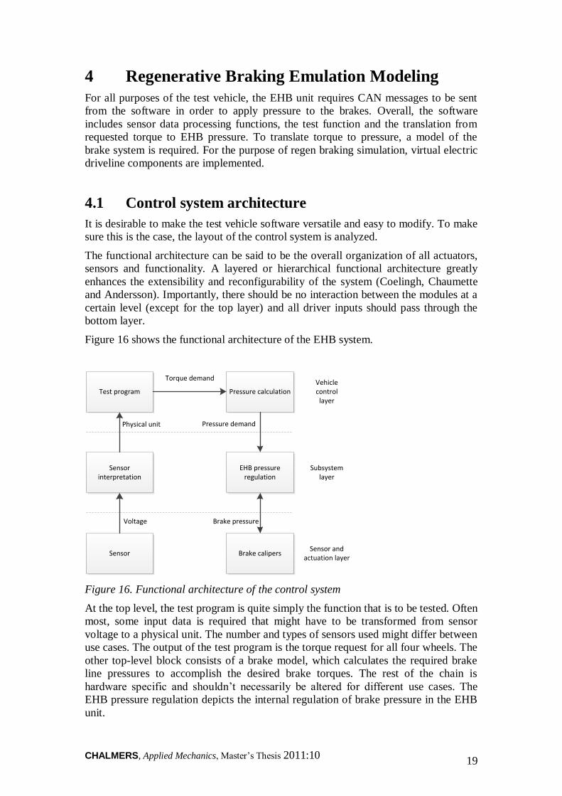
Figure 16 shows the functional architecture of the EHB system.
Sensor
Sensor interpretation
Test program Pressure calculation
EHB pressure regulation
Brake calipers
Torque demand
Voltage
Physical unit Pressure demand
Brake pressure
Vehicle control
layer
Subsystem layer
Sensor and actuation layer
Figure 16. Functional architecture of the control system
At the top level, the test program is quite simply the function that is to be tested. Often
most, some input data is required that might have to be transformed from sensor
voltage to a physical unit. The number and types of sensors used might differ between
use cases. The output of the test program is the torque request for all four wheels. The
other top-level block consists of a brake model, which calculates the required brake
line pressures to accomplish the desired brake torques. The rest of the chain is
hardware specific and shouldn‟t necessarily be altered for different use cases. The
EHB pressure regulation depicts the internal regulation of brake pressure in the EHB
unit.
CHALMERS, Applied Mechanics, Master‟s Thesis 2011:10 20
4.2 Overview of modeled subsystems
All modeled vehicle subsystems are described using flowcharts due to their
complexity. These describe the flow of information and the functions used. Each
flowchart module is detailed according to Table Table .
Table 1. Flow chart block shapes and their descriptions
Shape Description
Inputs
Outputs
Processes, calculations, sub-models
Pre-defined parameters
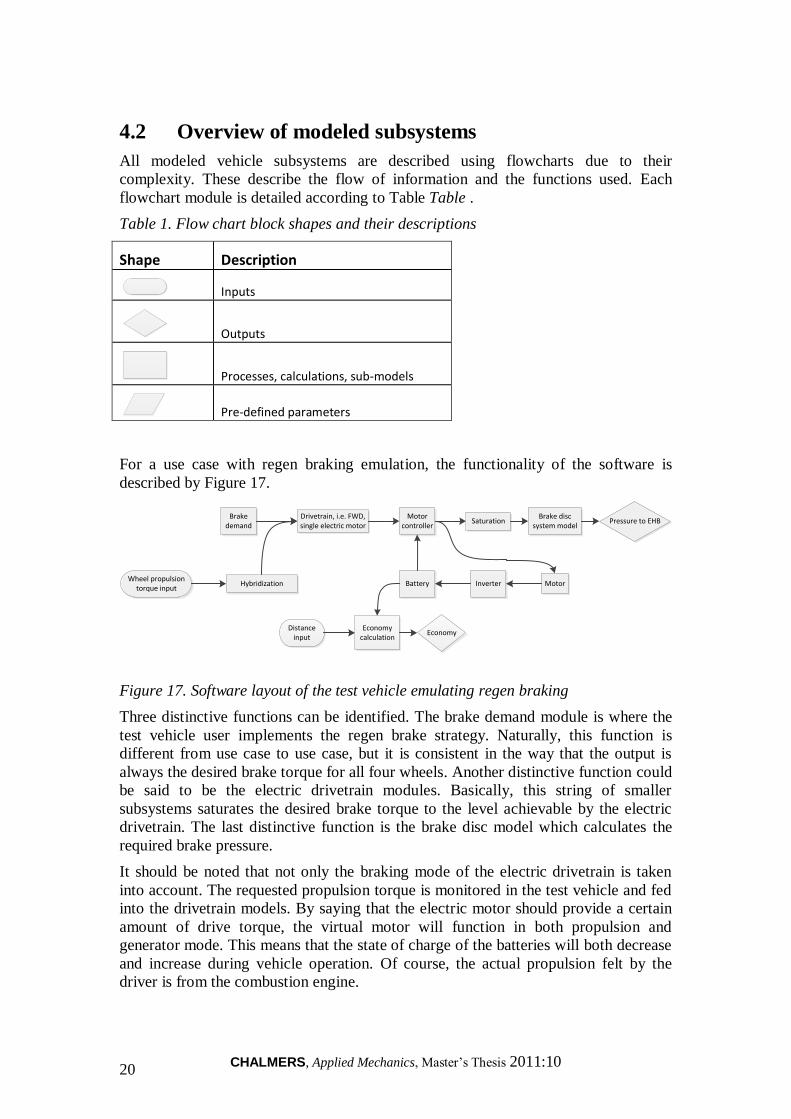
For a use case with regen braking emulation, the functionality of the software is
described by Figure 17.
Wheel propulsion torque input
Brake demand
Hybridization
Drivetrain, i.e. FWD, single electric motor
Motor controller
Battery Inverter Motor
SaturationBrake disc
system modelPressure to EHB
Economy calculation
EconomyDistance
input
Figure 17. Software layout of the test vehicle emulating regen braking
Three distinctive functions can be identified. The brake demand module is where the
test vehicle user implements the regen brake strategy. Naturally, this function is
different from use case to use case, but it is consistent in the way that the output is
always the desired brake torque for all four wheels. Another distinctive function could
be said to be the electric drivetrain modules. Basically, this string of smaller
subsystems saturates the desired brake torque to the level achievable by the electric
drivetrain. The last distinctive function is the brake disc model which calculates the
required brake pressure.
It should be noted that not only the braking mode of the electric drivetrain is taken
into account. The requested propulsion torque is monitored in the test vehicle and fed
into the drivetrain models. By saying that the electric motor should provide a certain
amount of drive torque, the virtual motor will function in both propulsion and
generator mode. This means that the state of charge of the batteries will both decrease
and increase during vehicle operation. Of course, the actual propulsion felt by the
driver is from the combustion engine.
CHALMERS, Applied Mechanics, Master‟s Thesis 2011:10 21
For software debugging of the test program, a vehicle simulation module is
implemented. This is described in Chapter 6.1.
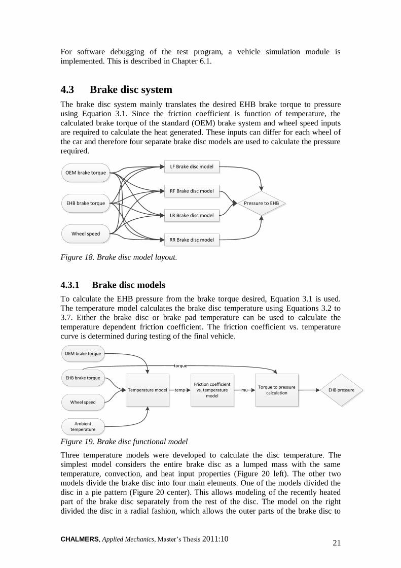
4.3 Brake disc system
The brake disc system mainly translates the desired EHB brake torque to pressure
using Equation 3.1. Since the friction coefficient is function of temperature, the
calculated brake torque of the standard (OEM) brake system and wheel speed inputs
are required to calculate the heat generated. These inputs can differ for each wheel of
the car and therefore four separate brake disc models are used to calculate the pressure
required.
OEM brake torque
EHB brake torque
Wheel speed
LF Brake disc model
Pressure to EHB
RF Brake disc model
LR Brake disc model
RR Brake disc model
Figure 18. Brake disc model layout.
4.3.1 Brake disc models
To calculate the EHB pressure from the brake torque desired, Equation 3.1 is used.
The temperature model calculates the brake disc temperature using Equations 3.2 to
3.7. Either the brake disc or brake pad temperature can be used to calculate the
temperature dependent friction coefficient. The friction coefficient vs. temperature
curve is determined during testing of the final vehicle.
OEM brake torque
EHB brake torque
Wheel speed
Ambient temperature
Temperature modelFriction coefficient
vs. temperature model
Torque to pressure calculation
EHB pressure
torque
temp mu
Figure 19. Brake disc functional model
Three temperature models were developed to calculate the disc temperature. The
simplest model considers the entire brake disc as a lumped mass with the same
temperature, convection, and heat input properties (Figure 20 left). The other two
models divide the brake disc into four main elements. One of the models divided the
disc in a pie pattern (Figure 20 center). This allows modeling of the recently heated
part of the brake disc separately from the rest of the disc. The model on the right
divided the disc in a radial fashion, which allows the outer parts of the brake disc to
CHALMERS, Applied Mechanics, Master‟s Thesis 2011:10 22
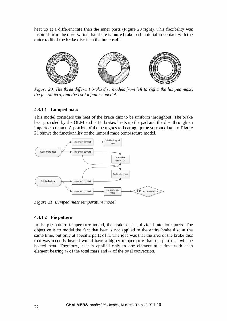
heat up at a different rate than the inner parts (Figure 20 right). This flexibility was
inspired from the observation that there is more brake pad material in contact with the
outer radii of the brake disc than the inner radii.
Figure 20. The three different brake disc models from left to right: the lumped mass,
the pie pattern, and the radial pattern model.
4.3.1.1 Lumped mass
This model considers the heat of the brake disc to be uniform throughout. The brake
heat provided by the OEM and EHB brakes heats up the pad and the disc through an
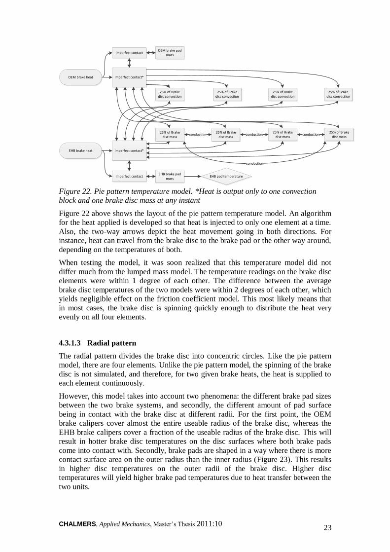
imperfect contact. A portion of the heat goes to heating up the surrounding air. Figure
21 shows the functionality of the lumped mass temperature model.
Figure 21. Lumped mass temperature model
4.3.1.2 Pie pattern
In the pie pattern temperature model, the brake disc is divided into four parts. The
objective is to model the fact that heat is not applied to the entire brake disc at the
same time, but only at specific parts of it. The idea was that the area of the brake disc
that was recently heated would have a higher temperature than the part that will be
heated next. Therefore, heat is applied only to one element at a time with each
element bearing ¼ of the total mass and ¼ of the total convection.
CHALMERS, Applied Mechanics, Master‟s Thesis 2011:10 23
Imperfect contact
OEM brake heat
EHB brake heat
Imperfect contact*
Imperfect contact*
Imperfect contact
OEM brake pad mass
25% of Brake disc convection
25% of Brake disc mass
EHB brake pad mass
25% of Brake disc convection
25% of Brake disc mass
25% of Brake disc convection
25% of Brake disc mass
25% of Brake disc convection
25% of Brake disc mass
EHB pad temperature
conduction conduction conduction
conduction
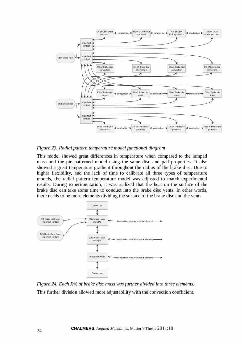
Figure 22. Pie pattern temperature model. *Heat is output only to one convection
block and one brake disc mass at any instant
Figure 22 above shows the layout of the pie pattern temperature model. An algorithm
for the heat applied is developed so that heat is injected to only one element at a time.
Also, the two-way arrows depict the heat movement going in both directions. For
instance, heat can travel from the brake disc to the brake pad or the other way around,
depending on the temperatures of both.
When testing the model, it was soon realized that this temperature model did not
differ much from the lumped mass model. The temperature readings on the brake disc
elements were within 1 degree of each other. The difference between the average
brake disc temperatures of the two models were within 2 degrees of each other, which
yields negligible effect on the friction coefficient model. This most likely means that
in most cases, the brake disc is spinning quickly enough to distribute the heat very
evenly on all four elements.
4.3.1.3 Radial pattern
The radial pattern divides the brake disc into concentric circles. Like the pie pattern
model, there are four elements. Unlike the pie pattern model, the spinning of the brake
disc is not simulated, and therefore, for two given brake heats, the heat is supplied to
each element continuously.
However, this model takes into account two phenomena: the different brake pad sizes
between the two brake systems, and secondly, the different amount of pad surface
being in contact with the brake disc at different radii. For the first point, the OEM
brake calipers cover almost the entire useable radius of the brake disc, whereas the
EHB brake calipers cover a fraction of the useable radius of the brake disc. This will
result in hotter brake disc temperatures on the disc surfaces where both brake pads
come into contact with. Secondly, brake pads are shaped in a way where there is more
contact surface area on the outer radius than the inner radius (Figure 23). This results
in higher disc temperatures on the outer radii of the brake disc. Higher disc
temperatures will yield higher brake pad temperatures due to heat transfer between the
two units.
CHALMERS, Applied Mechanics, Master‟s Thesis 2011:10 24
OEM brake heat
EHB brake heat
Imperfect contact
Imperfect contact
A% of Brake disc convection
A% of Brake disc mass
B% of Brake disc convection
B% of Brake disc mass
C% of Brake disc convection
C% of Brake disc mass
D% of Brake disc convection
D% of Brake disc mass
conduction conduction conduction
Imperfect contact
E% of OEM brake pad mass
F% of OEM brake pad mass
G% of OEM brake pad mass
H% of OEM brake pad mass
J% of EHB brake pad mass
K% of EHB brake pad mass
L% of EHB brake pad mass
M% of EHB brake pad mass
Imperfect contact
conduction conduction conduction
conduction conduction conduction
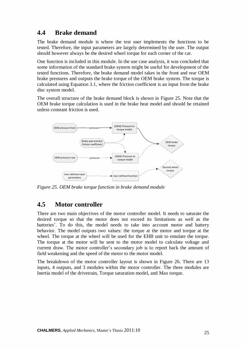
Figure 23. Radial pattern temperature model functional diagram
This model showed great differences in temperature when compared to the lumped
mass and the pie patterned model using the same disc and pad properties. It also
showed a great temperature gradient throughout the radius of the brake disc. Due to
higher flexibility, and the lack of time to calibrate all three types of temperature
models, the radial pattern temperature model was adjusted to match experimental
results. During experimentation, it was realized that the heat on the surface of the
brake disc can take some time to conduct into the brake disc vents. In other words,
there needs to be more elements dividing the surface of the brake disc and the vents.
EHB brake heat from imperfect contact
OEM brake heat from imperfect contact
Brake vent mass
(Disc mass – vent mass)/2
(Disc mass – vent mass)/2
Convection
Convection
Conduction to adacent radial element
Conduction to adacent radial element
Conduction to adacent radial element
Figure 24. Each X% of brake disc mass was further divided into three elements.
This further division allowed more adjustability with the convection coefficient.
CHALMERS, Applied Mechanics, Master‟s Thesis 2011:10 25
4.4 Brake demand
The brake demand module is where the test user implements the functions to be
tested. Therefore, the input parameters are largely determined by the user. The output
should however always be the desired wheel torque for each corner of the car.
One function is included in this module. In the use case analysis, it was concluded that
some information of the standard brake system might be useful for development of the
tested functions. Therefore, the brake demand model takes in the front and rear OEM
brake pressures and outputs the brake torque of the OEM brake system. The torque is
calculated using Equation 3.1, where the friction coefficient is an input from the brake
disc system model.
The overall structure of the brake demand block is shown in Figure 25. Note that the
OEM brake torque calculation is used in the brake heat model and should be retained
unless constant friction is used.
OEM pressure front
Brake pad and disc friction coefficient
(OEM) Pressure to torque model
pressure
(OEM) Pressure to torque model
OEM brake torque
OEM pressure rear pressure
User-defined function
Desired wheel torque
User-defined input parameters
Figure 25. OEM brake torque function in brake demand module
4.5 Motor controller
There are two main objectives of the motor controller model. It needs to saturate the
desired torque so that the motor does not exceed its limitations as well as the
batteries‟. To do this, the model needs to take into account motor and battery
behavior. The model outputs two values: the torque at the motor and torque at the
wheel. The torque at the wheel will be used for the EHB unit to emulate the torque.
The torque at the motor will be sent to the motor model to calculate voltage and
current draw. The motor controller‟s secondary job is to report back the amount of
field weakening and the speed of the motor to the motor model.
The breakdown of the motor controller layout is shown in Figure 26. There are 13
inputs, 4 outputs, and 3 modules within the motor controller. The three modules are
Inertia model of the drivetrain, Torque saturation model, and Max torque.
CHALMERS, Applied Mechanics, Master‟s Thesis 2011:10 26
Battery Limit
Motor specification
Output to motor
Maximum rated motor current
Motor internal resistance
EMF constant
Torque constant
Reduction
Maximum battery charge current
Maximum battery discharge current
Maximum battery voltage
Wheel speed
Torque demand
Max allowabletorque at wheel
Motor inertia
Inertia model of the drivetrain
Drivetrain inertia
Accelerationor
braking
Torque saturation model
Torque demandIncluding inertial
effects
Weak field constant
Motor speed
Wheel speed
Torque at the wheel
Torque at the motor
Wheel to motor gearing conversion
Max Torque
Maximum motor current due to heat
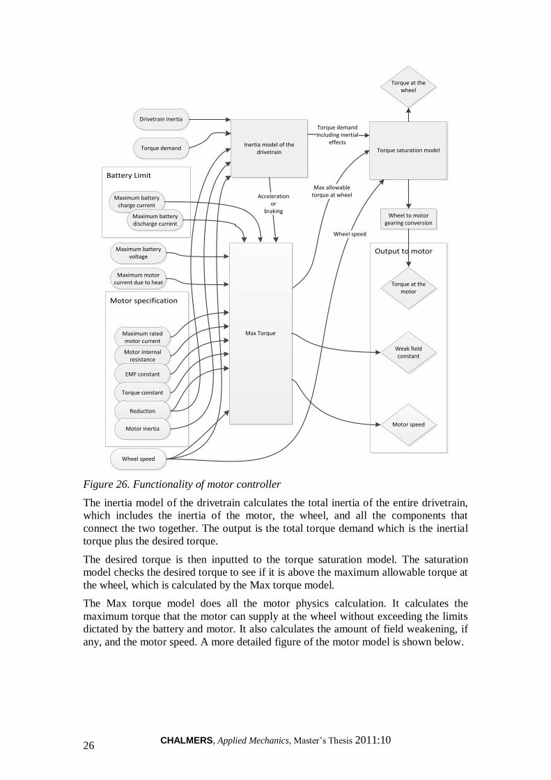
Figure 26. Functionality of motor controller
The inertia model of the drivetrain calculates the total inertia of the entire drivetrain,
which includes the inertia of the motor, the wheel, and all the components that
connect the two together. The output is the total torque demand which is the inertial
torque plus the desired torque.
The desired torque is then inputted to the torque saturation model. The saturation
model checks the desired torque to see if it is above the maximum allowable torque at
the wheel, which is calculated by the Max torque model.
The Max torque model does all the motor physics calculation. It calculates the
maximum torque that the motor can supply at the wheel without exceeding the limits
dictated by the battery and motor. It also calculates the amount of field weakening, if
any, and the motor speed. A more detailed figure of the motor model is shown below.

CHALMERS, Applied Mechanics, Master‟s Thesis 2011:10 27
Max torque
Battery Limit
Equation model
Motor specification
Maximum rated motor current
Motor internal resistance
EMF constant
Torque constant
Reduction
Maximum battery charge current
Maximum battery discharge current
Maximum battery voltage
Wheel speed
Wheel to motor gearing conversion
Field weakening model
Motor current limit due to supply
voltage in acceleration mode
Weak field or full field
Motor current limit due to supply
voltage in brake mode
Current saturation model
Torque demand
current
current
current
current
Current to torque conversion
Torque constant
Motor to wheel gearing conversion
reduction
Weak field constant
Motor inertia
Inertia model of the drivetrain
Drivetrain inertia
Accelerationor
braking
Max allowabletorque at wheel
Maximum motor current due to heat
current
Weak field constant
Motor speed
Figure 27. Motor behavior model
In this more detailed view, the Max torque model can be seen as a collection of the
equation model, the current saturation model, and the current to torque conversion
model. In the equation model, the motor current limit due to supply voltage in brake
and acceleration mode is calculated using Equation 3.10. The motor current limit due
to supply voltage in brake mode is also calculated using the same equation with V =
0. This is because a negative voltage will produce brake torque while expending
energy instead of regenerating it. The field weakening model calculates how much the
flux density should be decreased, if need be. It outputs a weak field constant which is
defined by the equation below, where 𝐸𝑝𝑒𝑎𝑘 is the highest amount of induced EMF
possible. This can be calculated using Equation 3.10 at the point boundary between
full field and weak field at maximum supply voltage.
𝑘𝑓 =𝐸𝑝𝑒𝑎𝑘
𝑘𝑒𝜔
The weak field constant, 𝑘𝑓 , can then be used elsewhere to derive the torque/current
relationship in the weak field region of the operating regions of the electric motor. All
the current limits are then inputted into the current saturation model to output the
lowest current limit, which would account for the rest of the current limits. Current to
torque conversion is done using Equation 3.13.
CHALMERS, Applied Mechanics, Master‟s Thesis 2011:10 28
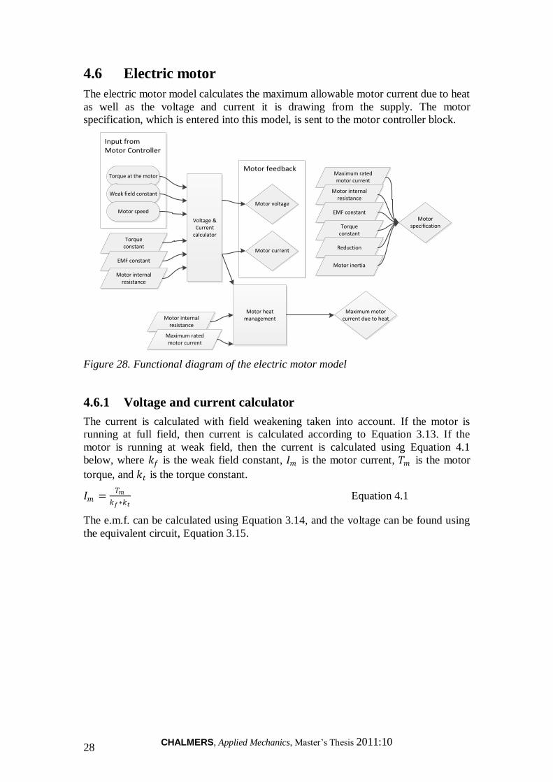
4.6 Electric motor
The electric motor model calculates the maximum allowable motor current due to heat
as well as the voltage and current it is drawing from the supply. The motor
specification, which is entered into this model, is sent to the motor controller block.
Input from Motor Controller
Motor feedbackTorque at the motor
Weak field constant
Motor speed
Torque constant
EMF constant
Motor internal resistance
Maximum rated motor current
Motor internal resistance
EMF constant
Torque constant
Reduction
Motor inertia
Voltage & Current
calculator
Motor heat managementMotor internal
resistance
Maximum rated motor current
Motor voltage
Motor current
Maximum motor current due to heat
Motor specification
Figure 28. Functional diagram of the electric motor model
4.6.1 Voltage and current calculator
The current is calculated with field weakening taken into account. If the motor is
running at full field, then current is calculated according to Equation 3.13. If the
motor is running at weak field, then the current is calculated using Equation 4.1
below, where 𝑘𝑓 is the weak field constant, 𝐼𝑚 is the motor current, 𝑇𝑚 is the motor
torque, and 𝑘𝑡 is the torque constant.
𝐼𝑚 =𝑇𝑚
𝑘𝑓∗𝑘𝑡 Equation 4.1
The e.m.f. can be calculated using Equation 3.14, and the voltage can be found using
the equivalent circuit, Equation 3.15.
CHALMERS, Applied Mechanics, Master‟s Thesis 2011:10 29
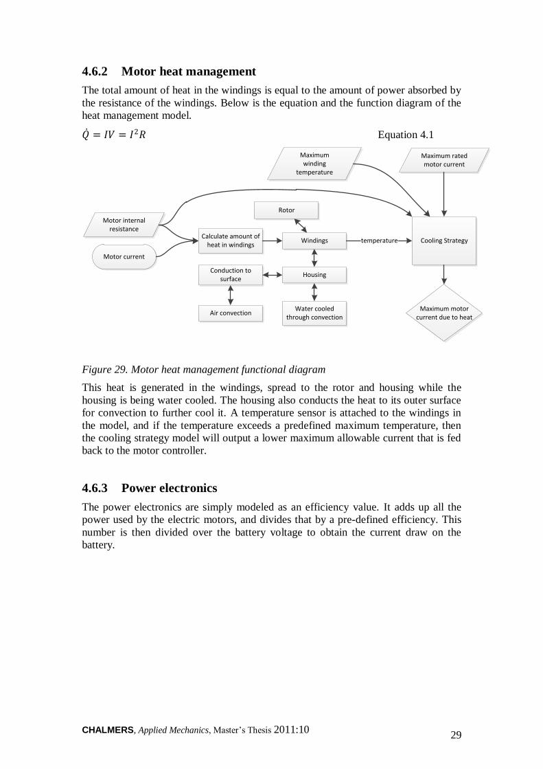
4.6.2 Motor heat management
The total amount of heat in the windings is equal to the amount of power absorbed by
the resistance of the windings. Below is the equation and the function diagram of the
heat management model.
𝑄 = 𝐼𝑉 = 𝐼2𝑅 Equation 4.1
Motor internal resistance
Maximum rated motor current
Maximum motor current due to heat
Motor current
Calculate amount of heat in windings
Windings
Rotor
HousingConduction to
surface
Water cooled through convection
Air convection
Cooling Strategytemperature
Maximum winding
temperature
Figure 29. Motor heat management functional diagram
This heat is generated in the windings, spread to the rotor and housing while the
housing is being water cooled. The housing also conducts the heat to its outer surface
for convection to further cool it. A temperature sensor is attached to the windings in
the model, and if the temperature exceeds a predefined maximum temperature, then
the cooling strategy model will output a lower maximum allowable current that is fed
back to the motor controller.
4.6.3 Power electronics
The power electronics are simply modeled as an efficiency value. It adds up all the
power used by the electric motors, and divides that by a pre-defined efficiency. This
number is then divided over the battery voltage to obtain the current draw on the
battery.
CHALMERS, Applied Mechanics, Master‟s Thesis 2011:10 30
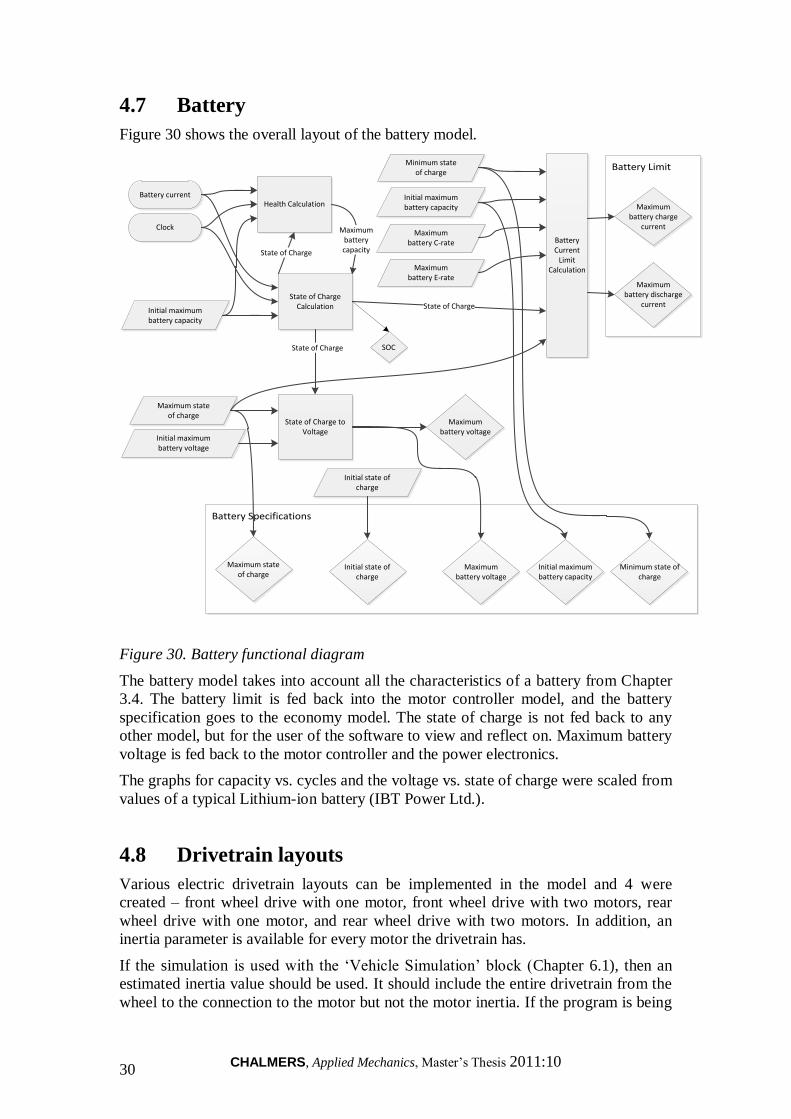
4.7 Battery
Figure 30 shows the overall layout of the battery model.
Battery Limit
Battery Specifications
Battery current
Clock
Initial maximum battery voltage
Minimum state of charge
Maximum battery C-rate
Maximum battery E-rate
Initial maximum battery capacity
Initial maximum battery capacity
Health Calculation
State of Charge Calculation
Maximumbatterycapacity
Battery Current
Limit Calculation
State of Charge
State of Charge
State of Charge to Voltage
State of Charge
Maximum state of charge
Maximum battery charge
current
Maximum battery discharge
current
Maximum battery voltage
Maximum battery voltage
Initial maximum battery capacity
Initial state of charge
Maximum state of charge
Minimum state of charge
Initial state of charge
SOC
Figure 30. Battery functional diagram
The battery model takes into account all the characteristics of a battery from Chapter
3.4. The battery limit is fed back into the motor controller model, and the battery
specification goes to the economy model. The state of charge is not fed back to any
other model, but for the user of the software to view and reflect on. Maximum battery
voltage is fed back to the motor controller and the power electronics.
The graphs for capacity vs. cycles and the voltage vs. state of charge were scaled from
values of a typical Lithium-ion battery (IBT Power Ltd.).
4.8 Drivetrain layouts
Various electric drivetrain layouts can be implemented in the model and 4 were
created – front wheel drive with one motor, front wheel drive with two motors, rear
wheel drive with one motor, and rear wheel drive with two motors. In addition, an
inertia parameter is available for every motor the drivetrain has.
If the simulation is used with the „Vehicle Simulation‟ block (Chapter 6.1), then an
estimated inertia value should be used. It should include the entire drivetrain from the
wheel to the connection to the motor but not the motor inertia. If the program is being
CHALMERS, Applied Mechanics, Master‟s Thesis 2011:10 31
used in the test vehicle, then no inertia should be used since the propulsion torque is
calculated from the measured engine torque, which includes the extra torque required
to overcome the inertia.
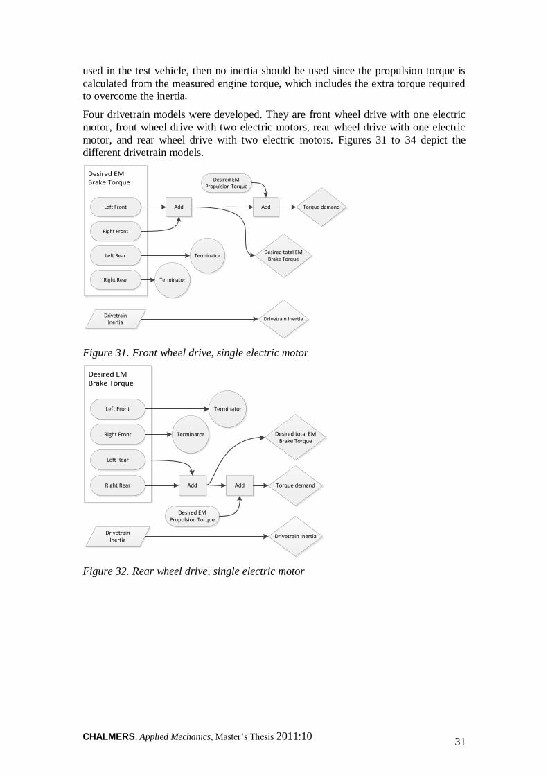
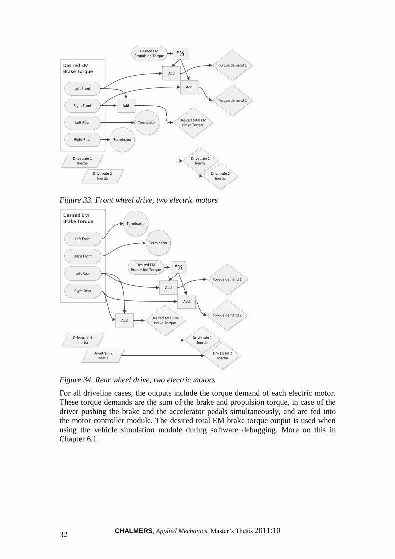
Four drivetrain models were developed. They are front wheel drive with one electric
motor, front wheel drive with two electric motors, rear wheel drive with one electric
motor, and rear wheel drive with two electric motors. Figures 31 to 34 depict the
different drivetrain models.
Desired EM Brake Torque
Left Front
Right Front
Left Rear
Right Rear
Desired EM Propulsion Torque
Add Add Torque demand
Drivetrain Inertia
Drivetrain Inertia
Terminator
Terminator
Desired total EM Brake Torque
Figure 31. Front wheel drive, single electric motor
Desired EM Brake Torque
Left Front
Right Front
Left Rear
Right Rear
Desired EM Propulsion Torque
Add Add Torque demand
Drivetrain Inertia
Drivetrain Inertia
Terminator
Terminator Desired total EM Brake Torque
Figure 32. Rear wheel drive, single electric motor
CHALMERS, Applied Mechanics, Master‟s Thesis 2011:10 32
Desired EM Brake Torque
Left Front
Right Front
Left Rear
Right Rear
Desired EM Propulsion Torque
Add
Torque demand 1
Drivetrain 1 Inertia
Drivetrain 1 Inertia
Terminator
Terminator
Desired total EM Brake Torque
Drivetrain 2 Inertia
Drivetrain 2 Inertia
*½
Torque demand 2
Add
Add
Figure 33. Front wheel drive, two electric motors
Desired EM Brake Torque
Left Front
Right Front
Left Rear
Right Rear
Desired EM Propulsion Torque
Add
Torque demand 1
Drivetrain 1 Inertia
Drivetrain 1 Inertia
Terminator
Terminator
Desired total EM Brake Torque
Drivetrain 2 Inertia
Drivetrain 2 Inertia
*½
Torque demand 2
Add
Add
Figure 34. Rear wheel drive, two electric motors
For all driveline cases, the outputs include the torque demand of each electric motor.
These torque demands are the sum of the brake and propulsion torque, in case of the
driver pushing the brake and the accelerator pedals simultaneously, and are fed into
the motor controller module. The desired total EM brake torque output is used when
using the vehicle simulation module during software debugging. More on this in
Chapter 6.1.
CHALMERS, Applied Mechanics, Master‟s Thesis 2011:10 33
4.8.1 Saturation layouts
Since the modeled electric drivetrain operates in both propulsion and regen mode, the
requested wheel torque might be positive (propulsion torque). Since the EHB system
naturally can‟t provide propulsion torque, the torque request from the motor controller
module is saturated so that only brake torque passes through. In short, it prepares the
torque values to be calculated into pressure at each wheel. It is drivetrain specific so
various saturation blocks are created for various drivetrain layouts.
4.9 Vehicle propulsion torque
A propulsion torque must be calculated in order to discharge the emulated battery. To
do this, Equation 4.3 was used where 𝑇𝑤 is the wheel torque, 𝑇𝑒 is the engine torque,
𝜔𝑒 is the engine speed, and 𝜔𝑤 is the wheel speed.
𝑇𝑤 = 𝑇𝑒 ∗𝜔𝑒
𝜔𝑤 Equation 4.3
The input is the torque demand for the engine, which is received from the engine
management system. The motor model has a gear ratio parameter which is relative to
the wheel speed, not the engine speed. Therefore, the variable of interest is wheel
torque instead of engine torque. By taking the ratio between the wheel speed and the
engine speed, the wheel propulsion torque is calculated. However, the equation does
not take into account the inertial loss of the drivetrain. Therefore, the actual torque at
the wheels is most likely a bit lower than the calculated one during transient
conditions.
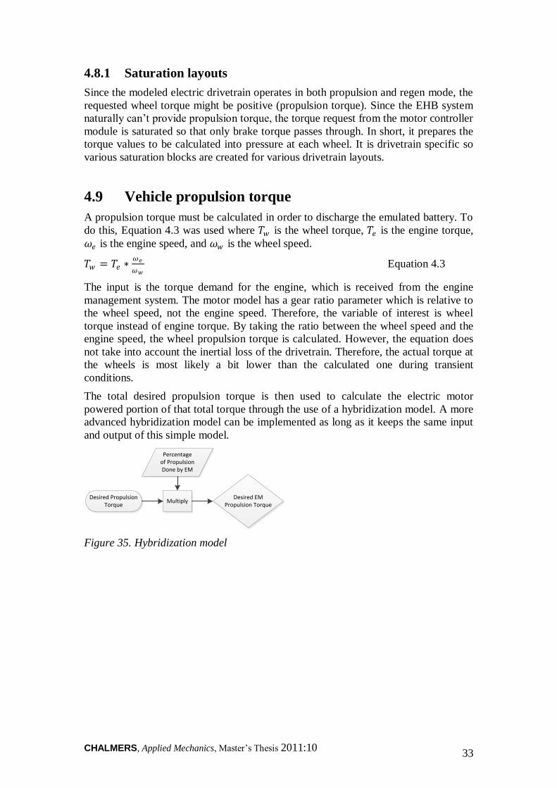
The total desired propulsion torque is then used to calculate the electric motor
powered portion of that total torque through the use of a hybridization model. A more
advanced hybridization model can be implemented as long as it keeps the same input
and output of this simple model.
Desired Propulsion Torque
Desired EM Propulsion Torque
Multiply
Percentage of Propulsion Done by EM
Figure 35. Hybridization model
CHALMERS, Applied Mechanics, Master‟s Thesis 2011:10 34
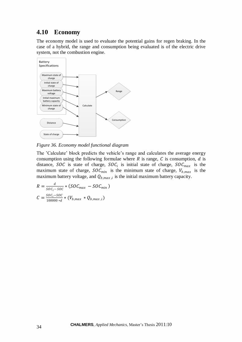
4.10 Economy
The economy model is used to evaluate the potential gains for regen braking. In the
case of a hybrid, the range and consumption being evaluated is of the electric drive
system, not the combustion engine.
Battery Specifications
Maximum state of charge
Initial state of charge
Maximum battery voltage
Initial maximum battery capacity
Minimum state of charge
Distance
State of charge
Range
Consumption
Calculate
Figure 36. Economy model functional diagram
The ‟Calculate‟ block predicts the vehicle‟s range and calculates the average energy
consumption using the following formulae where 𝑅 is range, 𝐶 is consumption, 𝑑 is
distance, 𝑆𝑂𝐶 is state of charge, 𝑆𝑂𝐶𝑖 is initial state of charge, 𝑆𝑂𝐶𝑚𝑎𝑥 is the
maximum state of charge, 𝑆𝑂𝐶𝑚𝑖𝑛 is the minimum state of charge, 𝑉𝑏 ,𝑚𝑎𝑥 is the
maximum battery voltage, and 𝑄𝑏 ,𝑚𝑎𝑥 ,𝑖 is the initial maximum battery capacity.
𝑅 =𝑑
𝑆𝑂𝐶𝑖− 𝑆𝑂𝐶∗ 𝑆𝑂𝐶𝑚𝑎𝑥 − 𝑆𝑂𝐶𝑚𝑖𝑛
𝐶 =𝑆𝑂𝐶𝑖−𝑆𝑂𝐶
100000 ∗𝑑∗ (𝑉𝑏 ,𝑚𝑎𝑥 ∗ 𝑄𝑏 ,𝑚𝑎𝑥 ,𝑖)
CHALMERS, Applied Mechanics, Master‟s Thesis 2011:10 35
5 Hardware Layout of the Test Vehicle
In this chapter, the hardware side of the test vehicle is introduced. To start with, the
base vehicle is depicted along with an overview of the modifications done and parts
added. Next, a safety analysis of the system is done. The EHB system is then
described further. The steering knuckle modifications and brake calipers
specifications are next dealt with. Lastly, the electric system is presented, including
signals, sensors and driver interface.
5.1 Overview
The base for the test vehicle is a 2008 SAAB 9-3. The car is equipped with a V6
Turbo engine and a manual gearbox. The specifications were chosen to be similar to
that of the current test vehicle at Chalmers, which will undergo the same
modifications as the SAAB car. By having the same equipment, the results gathered
by the two cars can be compared.
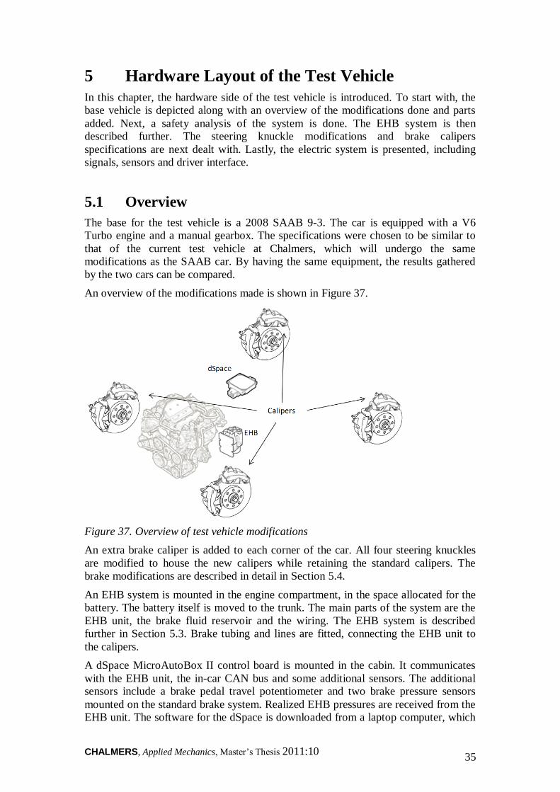
An overview of the modifications made is shown in Figure 37.
Figure 37. Overview of test vehicle modifications
An extra brake caliper is added to each corner of the car. All four steering knuckles
are modified to house the new calipers while retaining the standard calipers. The
brake modifications are described in detail in Section 5.4.
An EHB system is mounted in the engine compartment, in the space allocated for the
battery. The battery itself is moved to the trunk. The main parts of the system are the
EHB unit, the brake fluid reservoir and the wiring. The EHB system is described
further in Section 5.3. Brake tubing and lines are fitted, connecting the EHB unit to
the calipers.
A dSpace MicroAutoBox II control board is mounted in the cabin. It communicates
with the EHB unit, the in-car CAN bus and some additional sensors. The additional
sensors include a brake pedal travel potentiometer and two brake pressure sensors
mounted on the standard brake system. Realized EHB pressures are received from the
EHB unit. The software for the dSpace is downloaded from a laptop computer, which
CHALMERS, Applied Mechanics, Master‟s Thesis 2011:10 36
has a special computer table set up at the front passenger seat. Complementing the
computer controls is a box with physical switches, which activates/deactivates the
EHB system and provides configurable hardware functionality. The dSpace computer,
signal gathering and driver interface are all discussed in Section 5.5.
5.2 System safety analysis
In this section, an analysis of the system functions is done to ensure that the final
vehicle is safe to use on both the test track and public roads.
5.2.1 Safety requirements
The test vehicle will primarily be used on dedicated test tracks. An important
consideration is that it should still be capable of driving to and from the tracks on
public roads. This desire results in two major requirements on the test vehicle:
The original friction brake system should be retained, completely and without
modifications.
The EHB system can be totally electronically disengaged.
If fulfilled, these two requirements should enable the test vehicle to function exactly
as a standard vehicle when going on public roads.
While the safety in the transportation mode is reliant on keeping the standard vehicle
functions intact, the safety level during operating mode also depends on the
predictability of the added functions. Arguably, the precision of the functions is a
safety-related aspect. If the brake output differs in size, time response or any other
respect from the requested output, unwanted situations may occur. Having the system
properly calibrated is therefore not only of interest for precision in data sampling, but
also for the safety of the user. The calibration methods used for the test vehicle are
presented in chapter 0.
In a production car, safety-critical signals are made redundant, with observers
controlling the function. Due to the software type and the fact that the program is to
be modified by the end user, proper signal security is difficult to implement. For the
test vehicle software, the error handling is limited to making sure that the output
torque values are within the operation range of the EHB, and that they are saturated if
not.
A user guide is put together to inform the end user of precautions to take when using
the car. The aim is to provide a short, clear and informative paper with procedures for
both putting together new software models and executing them in the test vehicle.
The guide can be found in the vehicle.
5.2.2 Hazard analysis
Errors in a safety-critical system might lead to a hazard or, in worst case, a mishap.
The brake system implemented in the test vehicle is a safety-critical system.
Consequently, a systematic approach should be used to maintain the safety integrity of
the system. The engineering branch concerning risk management is called system
safety engineering. System safety should not be confused with reliability. The
CHALMERS, Applied Mechanics, Master‟s Thesis 2011:10 37
intention of system safety is not necessarily to minimize the number of breakdowns,
but rather to ensure that the effects of the breakdowns do not lead to hazards.
A part of system safety engineering is to identify, evaluate and control potential
hazards of the system, called hazard analysis. This approach was deemed to be
suitable to analyze the system safety of the test vehicle. It provides useful insights in
the system as a whole whilst being more manageable than the large effort of a
complete Failure Mode and Effects Analysis (FMEA) or a fault tree analysis. The
hazard analysis is consistent with the ISO 26262 “Road Vehicles – Functional
Standard”.
The hazard analysis was carried out in a number of steps. First, a block diagram of the
system and its boundaries was drawn. By understanding all involved parts and
functions, any unintended effects can be determined. The unintended effects were
compiled in a sheet, listing the parts/functions and the effect at different function
states; total loss, incorrect activation (more/less than expected or in the wrong
direction), unintended activation, or locked activation. Each effect was linked to one
or several hazards from a predefined list of vehicle hazards. Each hazard is in turn
associated with a risk. The risk scale is called ASIL and the value is determined from
the severity, likelihood and controllability of the hazard.
Two important conclusions were drawn from the analysis:
For functions that may lead to a complete or partial loss of brake torque,
falling back to the standard brake system is sufficient to avoid hazards.
The emergency switch needs to be able to disengage all functions that may
introduce unwanted brake torque and vehicle lateral motion, if no suitable
redundancy can be accomplished. Shutting down the EHB power is sufficient
to cover potential hazards.
Hence, the result of the hazard analysis is consistent with the requirements previously
put up in Section 5.2.1, as long as the emergency switch is able to completely
disengage the EHB system.
5.3 EHB system
The EHB system used is a Mercedes-Benz Sensotronic Brake Control (SBC) unit. It
was introduced in the 2003 SL-class (R230). Other models to use the SBC system is
the 2003-2005 E-class, CL, CLS, SLR and the Maybach. It was dropped in the high-
volume E-class due to reliability problems. The problems were related to the pump
motor being worn out on cars with high mileage or high frequency of brake operation.
The reliability issue is of long-term use nature and deemed not a problem for the test
vehicle.
5.3.1 Technical overview
One main feature of the selected system is the ability to adjust both front to rear and
side to side brake distribution. Effectively, this gives possibility to control each brake
caliper individually. Another feature is the precision and accuracy of the system. In
the vehicles using SBC, a so called soft-stop function is implemented. As the driver
brakes and the car approaches standstill, the brake pressure is gradually decreased to
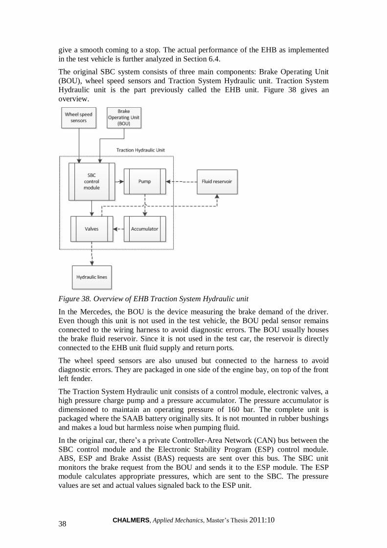
CHALMERS, Applied Mechanics, Master‟s Thesis 2011:10 38
give a smooth coming to a stop. The actual performance of the EHB as implemented
in the test vehicle is further analyzed in Section 6.4.
The original SBC system consists of three main components: Brake Operating Unit
(BOU), wheel speed sensors and Traction System Hydraulic unit. Traction System
Hydraulic unit is the part previously called the EHB unit. Figure 38 gives an
overview.
Figure 38. Overview of EHB Traction System Hydraulic unit
In the Mercedes, the BOU is the device measuring the brake demand of the driver.
Even though this unit is not used in the test vehicle, the BOU pedal sensor remains
connected to the wiring harness to avoid diagnostic errors. The BOU usually houses
the brake fluid reservoir. Since it is not used in the test car, the reservoir is directly
connected to the EHB unit fluid supply and return ports.
The wheel speed sensors are also unused but connected to the harness to avoid
diagnostic errors. They are packaged in one side of the engine bay, on top of the front
left fender.
The Traction System Hydraulic unit consists of a control module, electronic valves, a
high pressure charge pump and a pressure accumulator. The pressure accumulator is
dimensioned to maintain an operating pressure of 160 bar. The complete unit is
packaged where the SAAB battery originally sits. It is not mounted in rubber bushings
and makes a loud but harmless noise when pumping fluid.
In the original car, there‟s a private Controller-Area Network (CAN) bus between the
SBC control module and the Electronic Stability Program (ESP) control module.
ABS, ESP and Brake Assist (BAS) requests are sent over this bus. The SBC unit
monitors the brake request from the BOU and sends it to the ESP module. The ESP
module calculates appropriate pressures, which are sent to the SBC. The pressure
values are set and actual values signaled back to the ESP unit.

CHALMERS, Applied Mechanics, Master‟s Thesis 2011:10 39
In the test vehicle, the private CAN bus is taken over and used both to request brake
pressure and to gather information from the system. TNO, a Dutch technical research
institute, provided the software to achieve this. The availability of the TNO-software
was, together with the technical properties of the EHB system, the major reasons for
choosing the Mercedes SBC system for the test vehicle.
5.3.2 Hydraulic layout
The hydraulic layout of the original SBC system is displayed in Figure 39.
Figure 39. Hydraulic architecture of original SBC system
The SBC system consists of two hydraulic circuits; a main circuit and a backup
circuit. The backup circuit is engaged when errors occur or when the system is
switched off. Since the BOU is not connected, the supply line from the brake fluid
reservoir is split to feed brake fluid to the backup circuit. Components m1 and m3 is
the pump and pressure reservoir respectively. Components b1 to b6 are pressure
sensors. Component b2 monitors reservoir pressure and turns pump on/off to maintain
working pressure in the main circuit. Aside from measuring the brake pressure for
each corner, the brake pressure of the backup circuit is measured. Components y1 to
13 are control and balance valves. These are electronically controlled by the SBC
control module. There are three distinctive modes of operation; Pressure apply,
pressure hold and pressure release. In all cases, the inlet and outlet control valves are
energized in conjunction with the high pressure pump to give desired effect. By also
utilizing the balance valves, the brake pressures can be individually modulated.
5.3.3 Bleeding the EHB brakes
As usual, bleeding is done by connecting a pressure bleeder to the fluid reservoir and
opening the bleeder valves at the calipers. The EHB unit is turned on and off to get air
out of both the main and the backup circuit. Needless to say, the EHB unit has to be
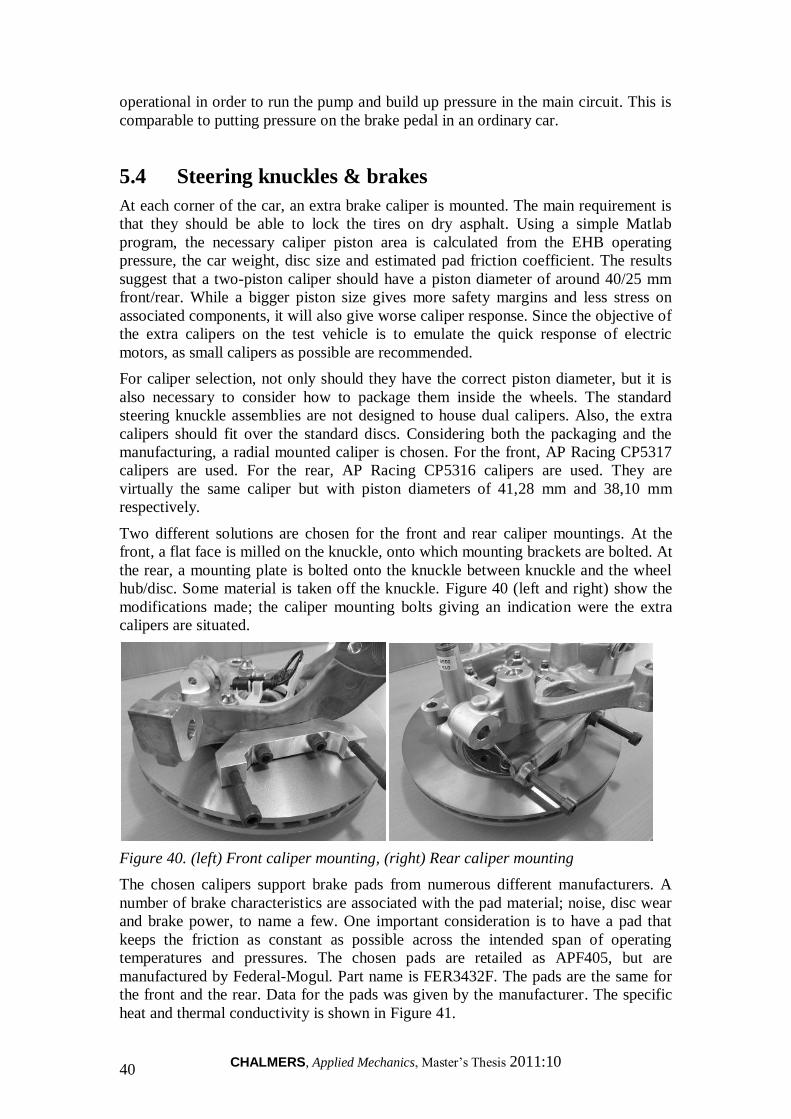
CHALMERS, Applied Mechanics, Master‟s Thesis 2011:10 40
operational in order to run the pump and build up pressure in the main circuit. This is
comparable to putting pressure on the brake pedal in an ordinary car.
5.4 Steering knuckles & brakes
At each corner of the car, an extra brake caliper is mounted. The main requirement is
that they should be able to lock the tires on dry asphalt. Using a simple Matlab
program, the necessary caliper piston area is calculated from the EHB operating
pressure, the car weight, disc size and estimated pad friction coefficient. The results
suggest that a two-piston caliper should have a piston diameter of around 40/25 mm
front/rear. While a bigger piston size gives more safety margins and less stress on
associated components, it will also give worse caliper response. Since the objective of
the extra calipers on the test vehicle is to emulate the quick response of electric
motors, as small calipers as possible are recommended.
For caliper selection, not only should they have the correct piston diameter, but it is
also necessary to consider how to package them inside the wheels. The standard
steering knuckle assemblies are not designed to house dual calipers. Also, the extra
calipers should fit over the standard discs. Considering both the packaging and the
manufacturing, a radial mounted caliper is chosen. For the front, AP Racing CP5317
calipers are used. For the rear, AP Racing CP5316 calipers are used. They are
virtually the same caliper but with piston diameters of 41,28 mm and 38,10 mm
respectively.
Two different solutions are chosen for the front and rear caliper mountings. At the
front, a flat face is milled on the knuckle, onto which mounting brackets are bolted. At
the rear, a mounting plate is bolted onto the knuckle between knuckle and the wheel
hub/disc. Some material is taken off the knuckle. Figure 40 (left and right) show the
modifications made; the caliper mounting bolts giving an indication were the extra
calipers are situated.
Figure 40. (left) Front caliper mounting, (right) Rear caliper mounting
The chosen calipers support brake pads from numerous different manufacturers. A
number of brake characteristics are associated with the pad material; noise, disc wear
and brake power, to name a few. One important consideration is to have a pad that
keeps the friction as constant as possible across the intended span of operating
temperatures and pressures. The chosen pads are retailed as APF405, but are
manufactured by Federal-Mogul. Part name is FER3432F. The pads are the same for
the front and the rear. Data for the pads was given by the manufacturer. The specific
heat and thermal conductivity is shown in Figure 41.
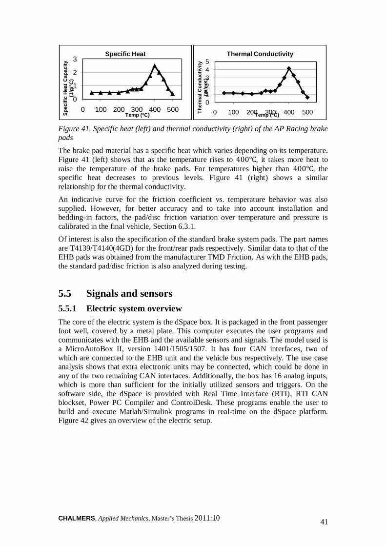
CHALMERS, Applied Mechanics, Master‟s Thesis 2011:10 41
Figure 41. Specific heat (left) and thermal conductivity (right) of the AP Racing brake
pads
The brake pad material has a specific heat which varies depending on its temperature.
Figure 41 (left) shows that as the temperature rises to 400℃, it takes more heat to
raise the temperature of the brake pads. For temperatures higher than 400℃, the
specific heat decreases to previous levels. Figure 41 (right) shows a similar
relationship for the thermal conductivity.
An indicative curve for the friction coefficient vs. temperature behavior was also
supplied. However, for better accuracy and to take into account installation and
bedding-in factors, the pad/disc friction variation over temperature and pressure is
calibrated in the final vehicle, Section 6.3.1.
Of interest is also the specification of the standard brake system pads. The part names
are T4139/T4140(4GD) for the front/rear pads respectively. Similar data to that of the
EHB pads was obtained from the manufacturer TMD Friction. As with the EHB pads,
the standard pad/disc friction is also analyzed during testing.
5.5 Signals and sensors
5.5.1 Electric system overview
The core of the electric system is the dSpace box. It is packaged in the front passenger
foot well, covered by a metal plate. This computer executes the user programs and
communicates with the EHB and the available sensors and signals. The model used is
a MicroAutoBox II, version 1401/1505/1507. It has four CAN interfaces, two of
which are connected to the EHB unit and the vehicle bus respectively. The use case
analysis shows that extra electronic units may be connected, which could be done in
any of the two remaining CAN interfaces. Additionally, the box has 16 analog inputs,
which is more than sufficient for the initially utilized sensors and triggers. On the
software side, the dSpace is provided with Real Time Interface (RTI), RTI CAN
blockset, Power PC Compiler and ControlDesk. These programs enable the user to
build and execute Matlab/Simulink programs in real-time on the dSpace platform.
Figure 42 gives an overview of the electric setup.
0
1
2
3
0 100 200 300 400 500
Sp
ecif
ic H
eat
Cap
acit
y
(J/g
/°C
)
Temp (°C)
Specific Heat
0
1
2
3
4
5
0 100 200 300 400 500Th
erm
al
Co
nd
ucti
vit
y
(W/m
K)
Temp (°C)
Thermal Conductivity
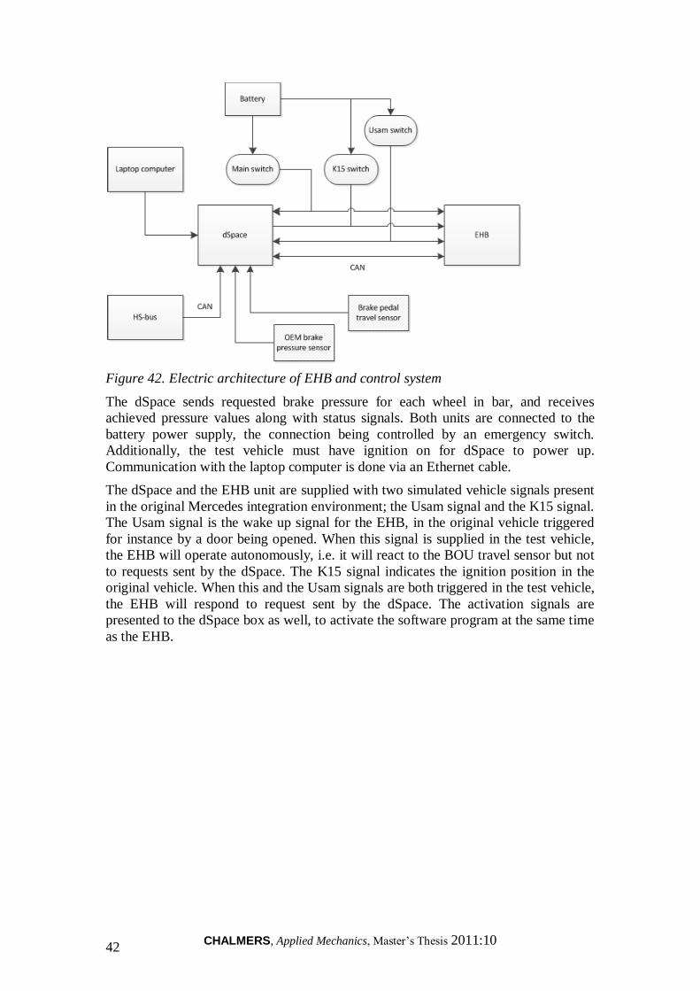
CHALMERS, Applied Mechanics, Master‟s Thesis 2011:10 42
Figure 42. Electric architecture of EHB and control system
The dSpace sends requested brake pressure for each wheel in bar, and receives
achieved pressure values along with status signals. Both units are connected to the
battery power supply, the connection being controlled by an emergency switch.
Additionally, the test vehicle must have ignition on for dSpace to power up.
Communication with the laptop computer is done via an Ethernet cable.
The dSpace and the EHB unit are supplied with two simulated vehicle signals present
in the original Mercedes integration environment; the Usam signal and the K15 signal.
The Usam signal is the wake up signal for the EHB, in the original vehicle triggered
for instance by a door being opened. When this signal is supplied in the test vehicle,
the EHB will operate autonomously, i.e. it will react to the BOU travel sensor but not
to requests sent by the dSpace. The K15 signal indicates the ignition position in the
original vehicle. When this and the Usam signals are both triggered in the test vehicle,
the EHB will respond to request sent by the dSpace. The activation signals are
presented to the dSpace box as well, to activate the software program at the same time
as the EHB.
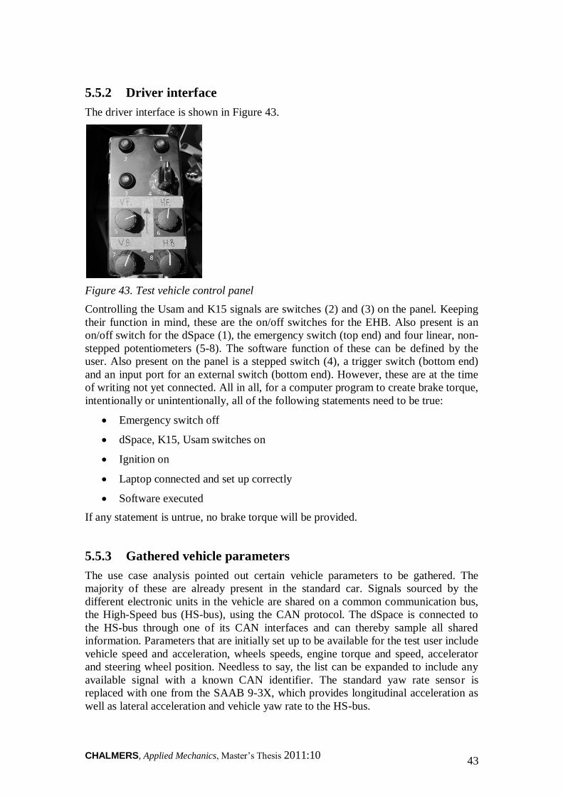
CHALMERS, Applied Mechanics, Master‟s Thesis 2011:10 43
5.5.2 Driver interface
The driver interface is shown in Figure 43.
Figure 43. Test vehicle control panel
Controlling the Usam and K15 signals are switches (2) and (3) on the panel. Keeping
their function in mind, these are the on/off switches for the EHB. Also present is an
on/off switch for the dSpace (1), the emergency switch (top end) and four linear, non-
stepped potentiometers (5-8). The software function of these can be defined by the
user. Also present on the panel is a stepped switch (4), a trigger switch (bottom end)
and an input port for an external switch (bottom end). However, these are at the time
of writing not yet connected. All in all, for a computer program to create brake torque,
intentionally or unintentionally, all of the following statements need to be true:
Emergency switch off
dSpace, K15, Usam switches on
Ignition on
Laptop connected and set up correctly
Software executed
If any statement is untrue, no brake torque will be provided.
5.5.3 Gathered vehicle parameters
The use case analysis pointed out certain vehicle parameters to be gathered. The
majority of these are already present in the standard car. Signals sourced by the
different electronic units in the vehicle are shared on a common communication bus,
the High-Speed bus (HS-bus), using the CAN protocol. The dSpace is connected to
the HS-bus through one of its CAN interfaces and can thereby sample all shared
information. Parameters that are initially set up to be available for the test user include
vehicle speed and acceleration, wheels speeds, engine torque and speed, accelerator
and steering wheel position. Needless to say, the list can be expanded to include any
available signal with a known CAN identifier. The standard yaw rate sensor is
replaced with one from the SAAB 9-3X, which provides longitudinal acceleration as
well as lateral acceleration and vehicle yaw rate to the HS-bus.
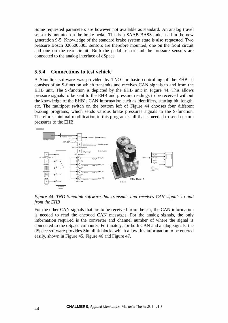
CHALMERS, Applied Mechanics, Master‟s Thesis 2011:10 44
Some requested parameters are however not available as standard. An analog travel
sensor is mounted on the brake pedal. This is a SAAB BASS unit, used in the new
generation 9-5. Knowledge of the standard brake system state is also requested. Two
pressure Bosch 0265005303 sensors are therefore mounted; one on the front circuit
and one on the rear circuit. Both the pedal sensor and the pressure sensors are
connected to the analog interface of dSpace.
5.5.4 Connections to test vehicle
A Simulink software was provided by TNO for basic controlling of the EHB. It
consists of an S-function which transmits and receives CAN signals to and from the
EHB unit. The S-function is depicted by the EHB unit in Figure 44. This allows
pressure signals to be sent to the EHB and pressure readings to be received without
the knowledge of the EHB‟s CAN information such as identifiers, starting bit, length,
etc. The multiport switch on the bottom left of Figure 44 chooses four different
braking programs, which sends various brake pressures signals to the S-function.
Therefore, minimal modification to this program is all that is needed to send custom
pressures to the EHB.
Figure 44. TNO Simulink software that transmits and receives CAN signals to and
from the EHB
For the other CAN signals that are to be received from the car, the CAN information
is needed to read the encoded CAN messages. For the analog signals, the only
information required is the converter and channel number of where the signal is
connected to the dSpace computer. Fortunately, for both CAN and analog signals, the
dSpace software provides Simulink blocks which allow this information to be entered
easily, shown in Figure 45, Figure 46 and Figure 47.
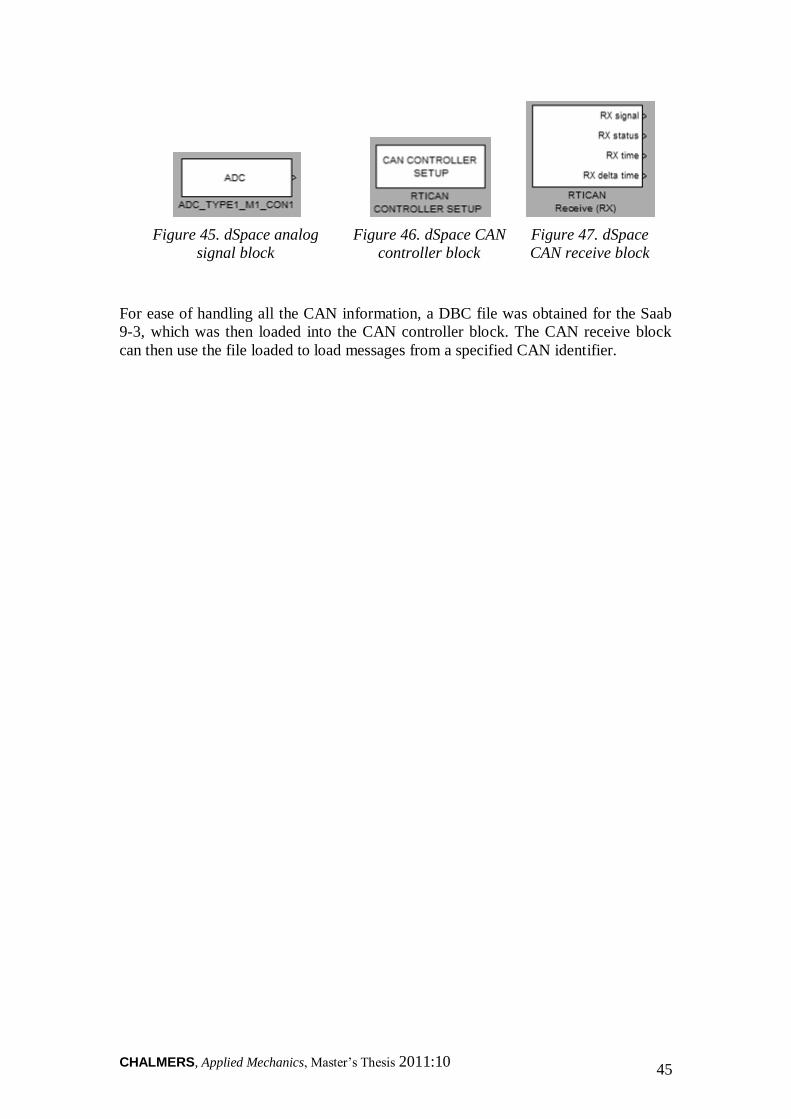
CHALMERS, Applied Mechanics, Master‟s Thesis 2011:10 45
Figure 45. dSpace analog
signal block
Figure 46. dSpace CAN
controller block
Figure 47. dSpace
CAN receive block
For ease of handling all the CAN information, a DBC file was obtained for the Saab
9-3, which was then loaded into the CAN controller block. The CAN receive block
can then use the file loaded to load messages from a specified CAN identifier.

CHALMERS, Applied Mechanics, Master‟s Thesis 2011:10 46
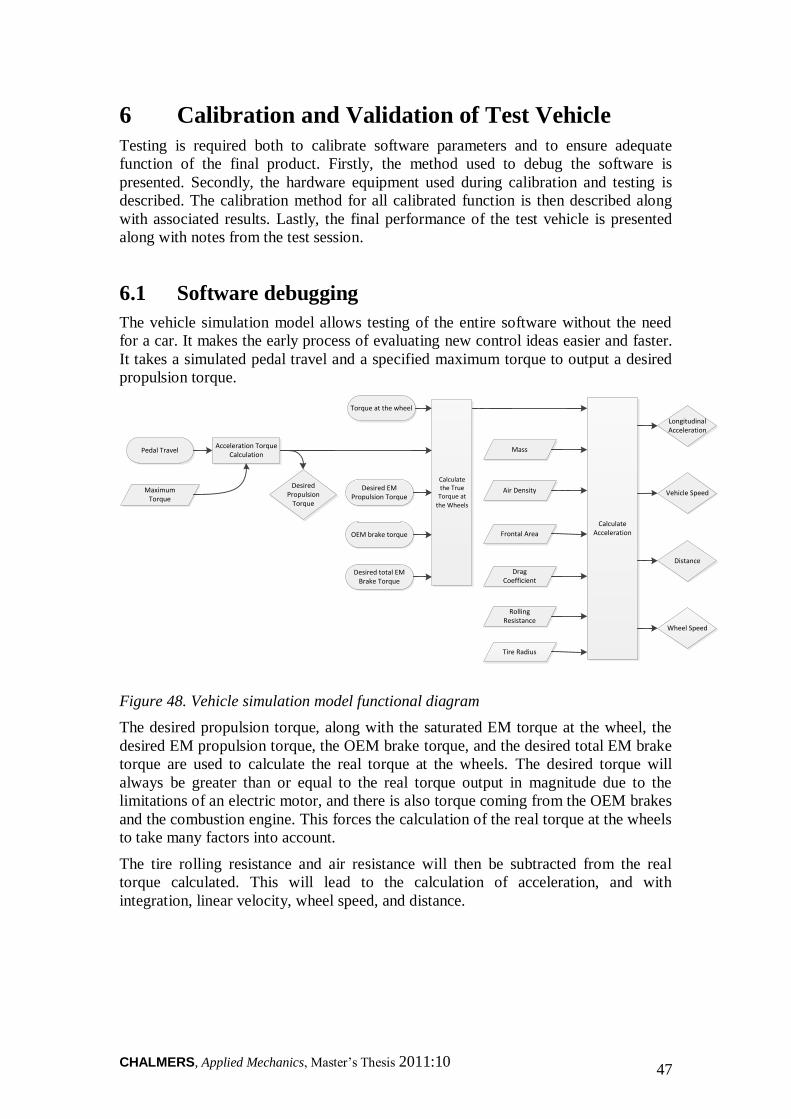
CHALMERS, Applied Mechanics, Master‟s Thesis 2011:10 47
6 Calibration and Validation of Test Vehicle
Testing is required both to calibrate software parameters and to ensure adequate
function of the final product. Firstly, the method used to debug the software is
presented. Secondly, the hardware equipment used during calibration and testing is
described. The calibration method for all calibrated function is then described along
with associated results. Lastly, the final performance of the test vehicle is presented
along with notes from the test session.
6.1 Software debugging
The vehicle simulation model allows testing of the entire software without the need
for a car. It makes the early process of evaluating new control ideas easier and faster.
It takes a simulated pedal travel and a specified maximum torque to output a desired
propulsion torque.
Pedal Travel
Maximum Torque
Acceleration Torque Calculation
Calculate the True
Torque at
the Wheels
Torque at the wheel
Desired EM Propulsion Torque
Desired Propulsion
Torque
OEM brake torque
Desired total EM Brake Torque
Calculate Acceleration
Mass
Air Density
Frontal Area
Drag Coefficient
Rolling Resistance
Tire Radius
Distance
Vehicle Speed
Longitudinal Acceleration
Wheel Speed
Figure 48. Vehicle simulation model functional diagram
The desired propulsion torque, along with the saturated EM torque at the wheel, the
desired EM propulsion torque, the OEM brake torque, and the desired total EM brake
torque are used to calculate the real torque at the wheels. The desired torque will
always be greater than or equal to the real torque output in magnitude due to the
limitations of an electric motor, and there is also torque coming from the OEM brakes
and the combustion engine. This forces the calculation of the real torque at the wheels
to take many factors into account.
The tire rolling resistance and air resistance will then be subtracted from the real
torque calculated. This will lead to the calculation of acceleration, and with
integration, linear velocity, wheel speed, and distance.
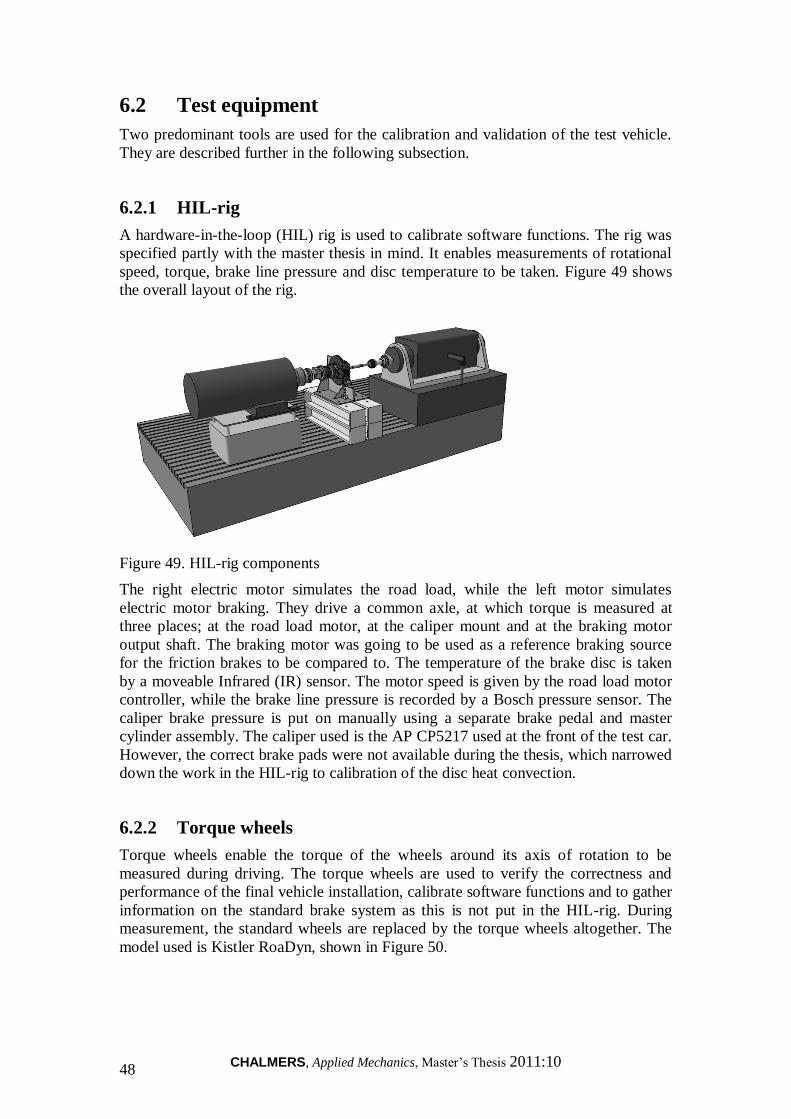
CHALMERS, Applied Mechanics, Master‟s Thesis 2011:10 48
6.2 Test equipment
Two predominant tools are used for the calibration and validation of the test vehicle.
They are described further in the following subsection.
6.2.1 HIL-rig
A hardware-in-the-loop (HIL) rig is used to calibrate software functions. The rig was
specified partly with the master thesis in mind. It enables measurements of rotational
speed, torque, brake line pressure and disc temperature to be taken. Figure 49 shows
the overall layout of the rig.
Figure 49. HIL-rig components
The right electric motor simulates the road load, while the left motor simulates
electric motor braking. They drive a common axle, at which torque is measured at
three places; at the road load motor, at the caliper mount and at the braking motor
output shaft. The braking motor was going to be used as a reference braking source
for the friction brakes to be compared to. The temperature of the brake disc is taken
by a moveable Infrared (IR) sensor. The motor speed is given by the road load motor
controller, while the brake line pressure is recorded by a Bosch pressure sensor. The
caliper brake pressure is put on manually using a separate brake pedal and master
cylinder assembly. The caliper used is the AP CP5217 used at the front of the test car.
However, the correct brake pads were not available during the thesis, which narrowed
down the work in the HIL-rig to calibration of the disc heat convection.
6.2.2 Torque wheels
Torque wheels enable the torque of the wheels around its axis of rotation to be
measured during driving. The torque wheels are used to verify the correctness and
performance of the final vehicle installation, calibrate software functions and to gather
information on the standard brake system as this is not put in the HIL-rig. During
measurement, the standard wheels are replaced by the torque wheels altogether. The
model used is Kistler RoaDyn, shown in Figure 50.
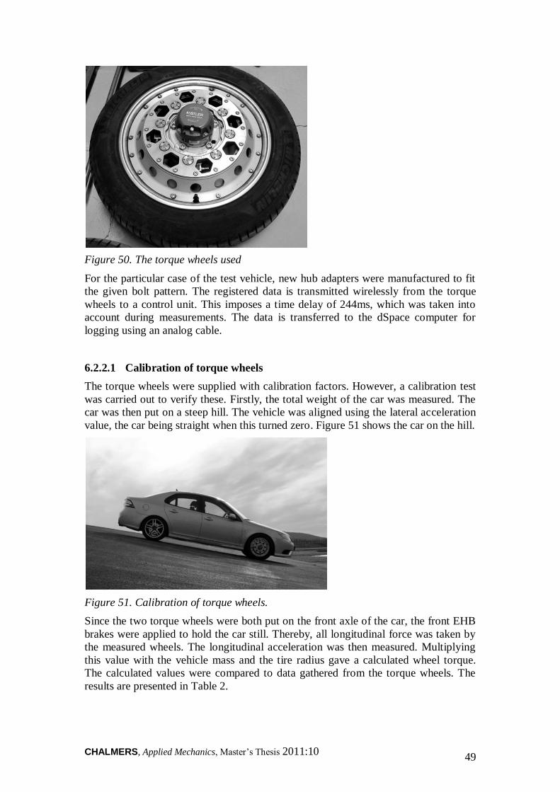
CHALMERS, Applied Mechanics, Master‟s Thesis 2011:10 49
Figure 50. The torque wheels used
For the particular case of the test vehicle, new hub adapters were manufactured to fit
the given bolt pattern. The registered data is transmitted wirelessly from the torque
wheels to a control unit. This imposes a time delay of 244ms, which was taken into
account during measurements. The data is transferred to the dSpace computer for
logging using an analog cable.
6.2.2.1 Calibration of torque wheels
The torque wheels were supplied with calibration factors. However, a calibration test
was carried out to verify these. Firstly, the total weight of the car was measured. The
car was then put on a steep hill. The vehicle was aligned using the lateral acceleration
value, the car being straight when this turned zero. Figure 51 shows the car on the hill.
Figure 51. Calibration of torque wheels.
Since the two torque wheels were both put on the front axle of the car, the front EHB
brakes were applied to hold the car still. Thereby, all longitudinal force was taken by
the measured wheels. The longitudinal acceleration was then measured. Multiplying
this value with the vehicle mass and the tire radius gave a calculated wheel torque.
The calculated values were compared to data gathered from the torque wheels. The
results are presented in Table 2.
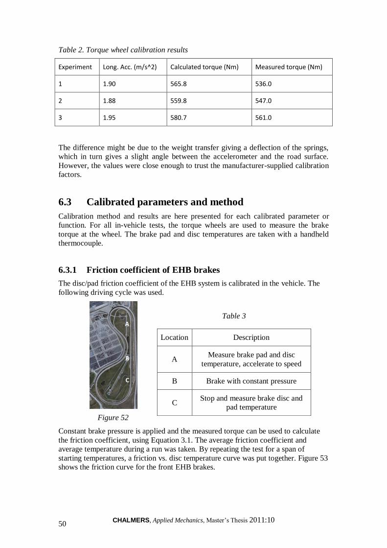
CHALMERS, Applied Mechanics, Master‟s Thesis 2011:10 50
Table 2. Torque wheel calibration results
Experiment Long. Acc. (m/s^2) Calculated torque (Nm) Measured torque (Nm)
1 1.90 565.8 536.0
2 1.88 559.8 547.0
3 1.95 580.7 561.0
The difference might be due to the weight transfer giving a deflection of the springs,
which in turn gives a slight angle between the accelerometer and the road surface.
However, the values were close enough to trust the manufacturer-supplied calibration
factors.
6.3 Calibrated parameters and method
Calibration method and results are here presented for each calibrated parameter or
function. For all in-vehicle tests, the torque wheels are used to measure the brake
torque at the wheel. The brake pad and disc temperatures are taken with a handheld
thermocouple.
6.3.1 Friction coefficient of EHB brakes
The disc/pad friction coefficient of the EHB system is calibrated in the vehicle. The
following driving cycle was used.
Figure 52
Table 3
Location Description
A Measure brake pad and disc
temperature, accelerate to speed
B Brake with constant pressure
C Stop and measure brake disc and
pad temperature
Constant brake pressure is applied and the measured torque can be used to calculate
the friction coefficient, using Equation 3.1. The average friction coefficient and
average temperature during a run was taken. By repeating the test for a span of
starting temperatures, a friction vs. disc temperature curve was put together. Figure 53
shows the friction curve for the front EHB brakes.
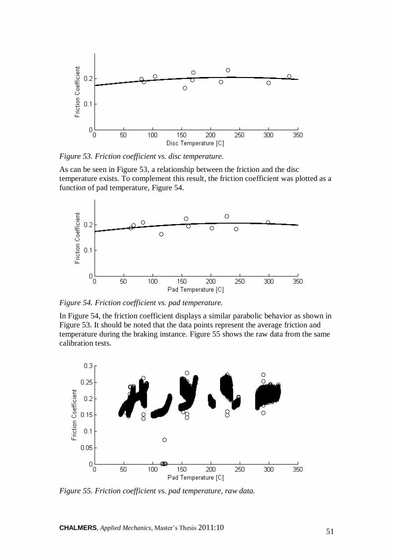
CHALMERS, Applied Mechanics, Master‟s Thesis 2011:10 51
Figure 53. Friction coefficient vs. disc temperature.
As can be seen in Figure 53, a relationship between the friction and the disc
temperature exists. To complement this result, the friction coefficient was plotted as a
function of pad temperature, Figure 54.
Figure 54. Friction coefficient vs. pad temperature.
In Figure 54, the friction coefficient displays a similar parabolic behavior as shown in
Figure 53. It should be noted that the data points represent the average friction and
temperature during the braking instance. Figure 55 shows the raw data from the same
calibration tests.
Figure 55. Friction coefficient vs. pad temperature, raw data.
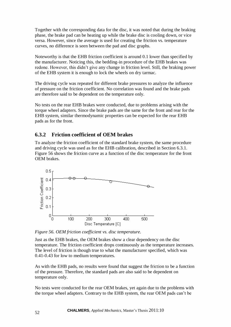
CHALMERS, Applied Mechanics, Master‟s Thesis 2011:10 52
Together with the corresponding data for the disc, it was noted that during the braking
phase, the brake pad can be heating up while the brake disc is cooling down, or vice
versa. However, since the average is used for creating the friction vs. temperature
curves, no difference is seen between the pad and disc graphs.
Noteworthy is that the EHB friction coefficient is around 0.1 lower than specified by
the manufacturer. Noticing this, the bedding-in procedure of the EHB brakes was
redone. However, this didn‟t give any change in friction level. Still, the braking power
of the EHB system it is enough to lock the wheels on dry tarmac.
The driving cycle was repeated for different brake pressures to analyze the influence
of pressure on the friction coefficient. No correlation was found and the brake pads
are therefore said to be dependent on the temperature only.
No tests on the rear EHB brakes were conducted, due to problems arising with the
torque wheel adapters. Since the brake pads are the same for the front and rear for the
EHB system, similar thermodynamic properties can be expected for the rear EHB
pads as for the front.
6.3.2 Friction coefficient of OEM brakes
To analyze the friction coefficient of the standard brake system, the same procedure
and driving cycle was used as for the EHB calibration, described in Section 6.3.1.
Figure 56 shows the friction curve as a function of the disc temperature for the front
OEM brakes.
Figure 56. OEM friction coefficient vs. disc temperature.
Just as the EHB brakes, the OEM brakes show a clear dependency on the disc
temperature. The friction coefficient drops continuously as the temperature increases.
The level of friction is though true to what the manufacturer specified, which was
0.41-0.43 for low to medium temperatures.
As with the EHB pads, no results were found that suggest the friction to be a function
of the pressure. Therefore, the standard pads are also said to be dependent on
temperature only.
No tests were conducted for the rear OEM brakes, yet again due to the problems with
the torque wheel adapters. Contrary to the EHB system, the rear OEM pads can‟t be
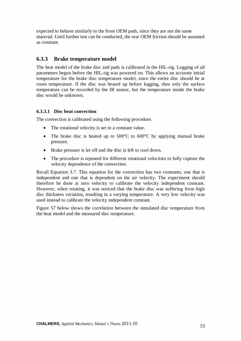
CHALMERS, Applied Mechanics, Master‟s Thesis 2011:10 53
expected to behave similarly to the front OEM pads, since they are not the same
material. Until further test can be conducted, the rear OEM friction should be assumed
as constant.
6.3.3 Brake temperature model
The heat model of the brake disc and pads is calibrated in the HIL-rig. Logging of all
parameters begun before the HIL-rig was powered on. This allows an accurate initial
temperature for the brake disc temperature model, since the entire disc should be at
room temperature. If the disc was heated up before logging, then only the surface
temperature can be recorded by the IR sensor, but the temperature inside the brake
disc would be unknown.
6.3.3.1 Disc heat convection
The convection is calibrated using the following procedure.
The rotational velocity is set to a constant value.
The brake disc is heated up to 500°C to 600°C by applying manual brake
pressure.
Brake pressure is let off and the disc is left to cool down.
The procedure is repeated for different rotational velocities to fully capture the
velocity dependence of the convection.
Recall Equation 3.7. This equation for the convection has two constants, one that is
independent and one that is dependent on the air velocity. The experiment should
therefore be done at zero velocity to calibrate the velocity independent constant.
However, when rotating, it was noticed that the brake disc was suffering from high
disc thickness variation, resulting in a varying temperature. A very low velocity was
used instead to calibrate the velocity independent constant.
Figure 57 below shows the correlation between the simulated disc temperature from
the heat model and the measured disc temperature.
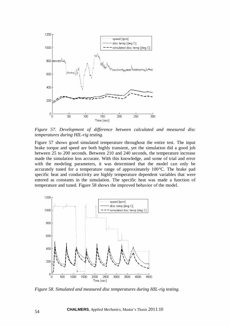
CHALMERS, Applied Mechanics, Master‟s Thesis 2011:10 54
Figure 57. Development of difference between calculated and measured disc
temperatures during HIL-rig testing.
Figure 57 shows good simulated temperature throughout the entire test. The input
brake torque and speed are both highly transient, yet the simulation did a good job
between 25 to 200 seconds. Between 210 and 240 seconds, the temperature increase
made the simulation less accurate. With this knowledge, and some of trial and error
with the modeling parameters, it was determined that the model can only be
accurately tuned for a temperature range of approximately 100°C. The brake pad
specific heat and conductivity are highly temperature dependent variables that were
entered as constants in the simulation. The specific heat was made a function of
temperature and tuned. Figure 58 shows the improved behavior of the model.
Figure 58. Simulated and measured disc temperatures during HIL-rig testing.
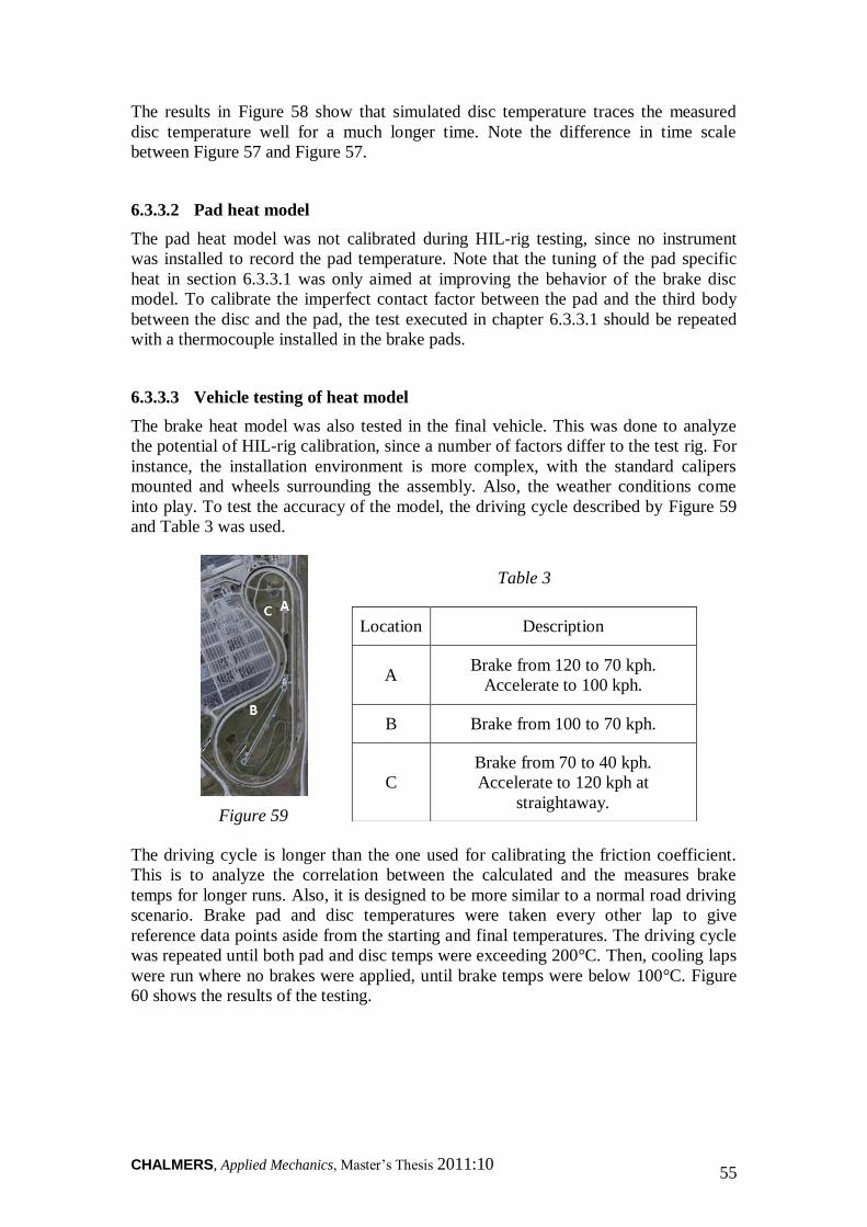
CHALMERS, Applied Mechanics, Master‟s Thesis 2011:10 55
The results in Figure 58 show that simulated disc temperature traces the measured
disc temperature well for a much longer time. Note the difference in time scale
between Figure 57 and Figure 57.
6.3.3.2 Pad heat model
The pad heat model was not calibrated during HIL-rig testing, since no instrument
was installed to record the pad temperature. Note that the tuning of the pad specific
heat in section 6.3.3.1 was only aimed at improving the behavior of the brake disc
model. To calibrate the imperfect contact factor between the pad and the third body
between the disc and the pad, the test executed in chapter 6.3.3.1 should be repeated
with a thermocouple installed in the brake pads.
6.3.3.3 Vehicle testing of heat model
The brake heat model was also tested in the final vehicle. This was done to analyze
the potential of HIL-rig calibration, since a number of factors differ to the test rig. For
instance, the installation environment is more complex, with the standard calipers
mounted and wheels surrounding the assembly. Also, the weather conditions come
into play. To test the accuracy of the model, the driving cycle described by Figure 59
and Table 3 was used.
Figure 59
Table 3
Location Description
A Brake from 120 to 70 kph.
Accelerate to 100 kph.
B Brake from 100 to 70 kph.
C
Brake from 70 to 40 kph.
Accelerate to 120 kph at
straightaway.
The driving cycle is longer than the one used for calibrating the friction coefficient.
This is to analyze the correlation between the calculated and the measures brake
temps for longer runs. Also, it is designed to be more similar to a normal road driving
scenario. Brake pad and disc temperatures were taken every other lap to give
reference data points aside from the starting and final temperatures. The driving cycle
was repeated until both pad and disc temps were exceeding 200°C. Then, cooling laps
were run where no brakes were applied, until brake temps were below 100°C. Figure
60 shows the results of the testing.
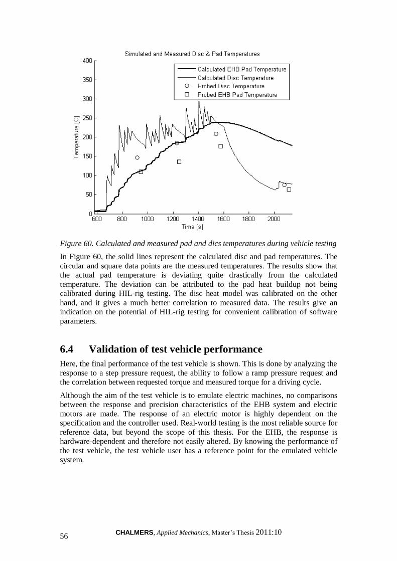
CHALMERS, Applied Mechanics, Master‟s Thesis 2011:10 56
Figure 60. Calculated and measured pad and dics temperatures during vehicle testing
In Figure 60, the solid lines represent the calculated disc and pad temperatures. The
circular and square data points are the measured temperatures. The results show that
the actual pad temperature is deviating quite drastically from the calculated
temperature. The deviation can be attributed to the pad heat buildup not being
calibrated during HIL-rig testing. The disc heat model was calibrated on the other
hand, and it gives a much better correlation to measured data. The results give an
indication on the potential of HIL-rig testing for convenient calibration of software
parameters.
6.4 Validation of test vehicle performance
Here, the final performance of the test vehicle is shown. This is done by analyzing the
response to a step pressure request, the ability to follow a ramp pressure request and
the correlation between requested torque and measured torque for a driving cycle.
Although the aim of the test vehicle is to emulate electric machines, no comparisons
between the response and precision characteristics of the EHB system and electric
motors are made. The response of an electric motor is highly dependent on the
specification and the controller used. Real-world testing is the most reliable source for
reference data, but beyond the scope of this thesis. For the EHB, the response is
hardware-dependent and therefore not easily altered. By knowing the performance of
the test vehicle, the test vehicle user has a reference point for the emulated vehicle
system.
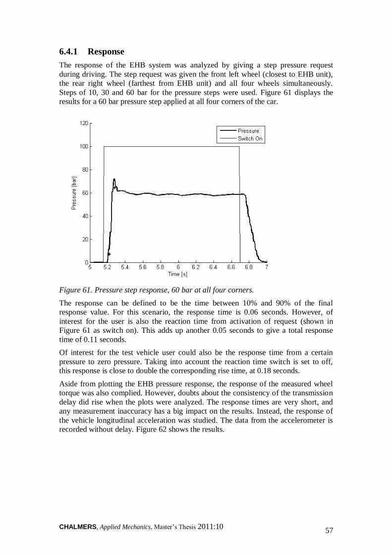
CHALMERS, Applied Mechanics, Master‟s Thesis 2011:10 57
6.4.1 Response
The response of the EHB system was analyzed by giving a step pressure request
during driving. The step request was given the front left wheel (closest to EHB unit),
the rear right wheel (farthest from EHB unit) and all four wheels simultaneously.
Steps of 10, 30 and 60 bar for the pressure steps were used. Figure 61 displays the
results for a 60 bar pressure step applied at all four corners of the car.
Figure 61. Pressure step response, 60 bar at all four corners.
The response can be defined to be the time between 10% and 90% of the final
response value. For this scenario, the response time is 0.06 seconds. However, of
interest for the user is also the reaction time from activation of request (shown in
Figure 61 as switch on). This adds up another 0.05 seconds to give a total response
time of 0.11 seconds.
Of interest for the test vehicle user could also be the response time from a certain
pressure to zero pressure. Taking into account the reaction time switch is set to off,
this response is close to double the corresponding rise time, at 0.18 seconds.
Aside from plotting the EHB pressure response, the response of the measured wheel
torque was also complied. However, doubts about the consistency of the transmission
delay did rise when the plots were analyzed. The response times are very short, and
any measurement inaccuracy has a big impact on the results. Instead, the response of
the vehicle longitudinal acceleration was studied. The data from the accelerometer is
recorded without delay. Figure 62 shows the results.

CHALMERS, Applied Mechanics, Master‟s Thesis 2011:10 58
Figure 62. Longitudinal acceleration step response, 60 bar at all four corners.
The response of the vehicle acceleration is very close in magnitude to the pressure
response. This indicates that the wheel torque response is likely very close to the EHB
pressure response.
6.4.2 Precision to ramp input
The internal pressure regulation of the EHB unit is analyzed using a pressure request
ramp. The ramp is set to increase at a rate of 5 bars per second until the vehicle stops.
The test is done twice; for one wheel only and for all wheels simultaneously. Figure
63 and Figure 64 show the results of these two runs respectively.
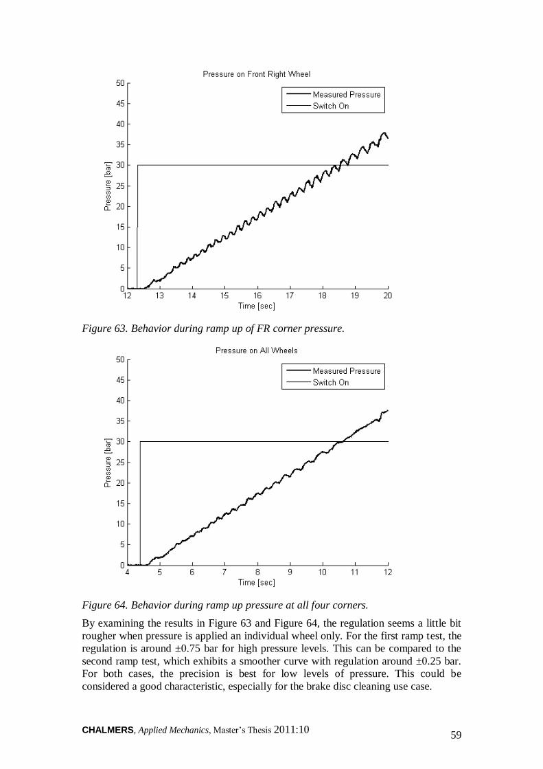
CHALMERS, Applied Mechanics, Master‟s Thesis 2011:10 59
Figure 63. Behavior during ramp up of FR corner pressure.
Figure 64. Behavior during ramp up pressure at all four corners.
By examining the results in Figure 63 and Figure 64, the regulation seems a little bit
rougher when pressure is applied an individual wheel only. For the first ramp test, the
regulation is around ±0.75 bar for high pressure levels. This can be compared to the
second ramp test, which exhibits a smoother curve with regulation around ±0.25 bar.
For both cases, the precision is best for low levels of pressure. This could be
considered a good characteristic, especially for the brake disc cleaning use case.
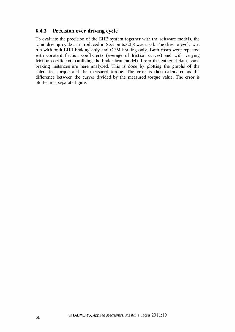
CHALMERS, Applied Mechanics, Master‟s Thesis 2011:10 60
6.4.3 Precision over driving cycle
To evaluate the precision of the EHB system together with the software models, the
same driving cycle as introduced in Section 6.3.3.3 was used. The driving cycle was
run with both EHB braking only and OEM braking only. Both cases were repeated
with constant friction coefficients (average of friction curves) and with varying
friction coefficients (utilizing the brake heat model). From the gathered data, some
braking instances are here analyzed. This is done by plotting the graphs of the
calculated torque and the measured torque. The error is then calculated as the
difference between the curves divided by the measured torque value. The error is
plotted in a separate figure.
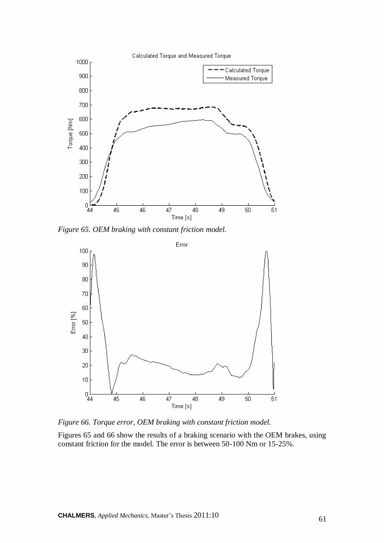
CHALMERS, Applied Mechanics, Master‟s Thesis 2011:10 61
Figure 65. OEM braking with constant friction model.
Figure 66. Torque error, OEM braking with constant friction model.
Figures 65 and 66 show the results of a braking scenario with the OEM brakes, using
constant friction for the model. The error is between 50-100 Nm or 15-25%.

CHALMERS, Applied Mechanics, Master‟s Thesis 2011:10 62
Figure 67. EHB braking with constant friction model.
Figure 68. Error, EHB braking with constant friction model.
Figures 67 and 68 show the results of a braking scenario with the EHB brakes, using
constant friction for the model. The error is between 40-80 Nm or 8-15%.
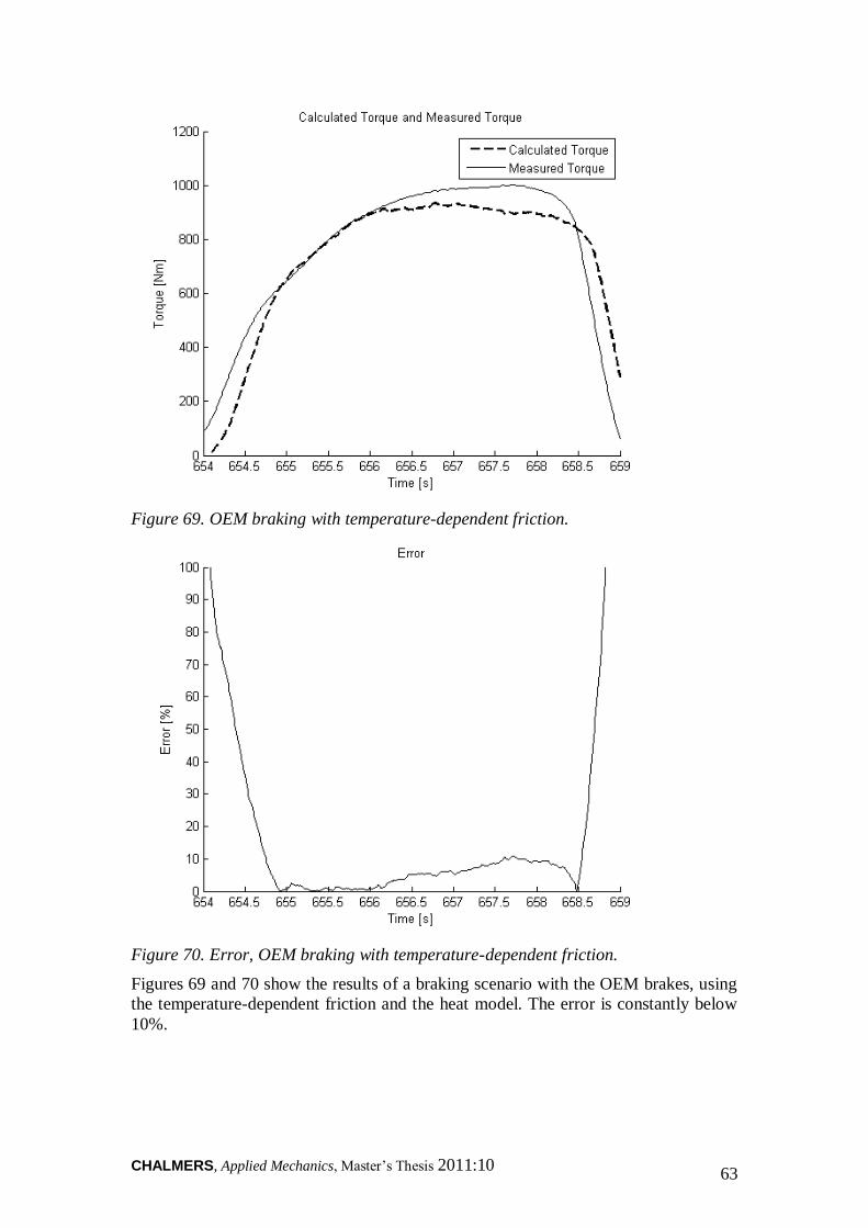
CHALMERS, Applied Mechanics, Master‟s Thesis 2011:10 63
Figure 69. OEM braking with temperature-dependent friction.
Figure 70. Error, OEM braking with temperature-dependent friction.
Figures 69 and 70 show the results of a braking scenario with the OEM brakes, using
the temperature-dependent friction and the heat model. The error is constantly below
10%.
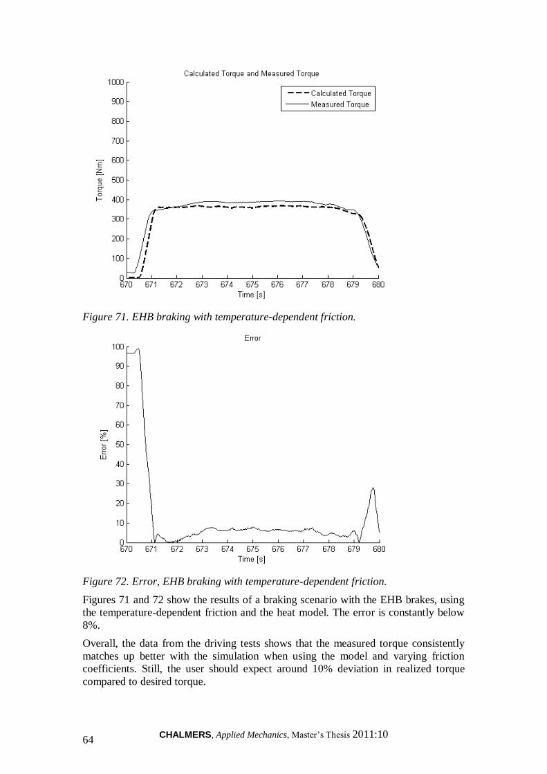
CHALMERS, Applied Mechanics, Master‟s Thesis 2011:10 64
Figure 71. EHB braking with temperature-dependent friction.
Figure 72. Error, EHB braking with temperature-dependent friction.
Figures 71 and 72 show the results of a braking scenario with the EHB brakes, using
the temperature-dependent friction and the heat model. The error is constantly below
8%.
Overall, the data from the driving tests shows that the measured torque consistently
matches up better with the simulation when using the model and varying friction
coefficients. Still, the user should expect around 10% deviation in realized torque
compared to desired torque.
CHALMERS, Applied Mechanics, Master‟s Thesis 2011:10 65
6.5 Notes from test driving
During testing, a transient behavior of the friction coefficient of both the EHB and the
OEM brake pads was observed. That is to say, a constant torque request would give a
wheel torque that deviated either linearly or exponentially from the intended value. To
capture this transient behavior in the software models, further HIL-rig calibration of
the brake heat model is required. Of main concern is the temperature buildup and
cool-down of the brake pads. With more insight in the brake disc-pad thermodynamic
interaction, the precision of the EHB system might be improved.
Recall the temperature-dependence of the specific heat and conductivity of the EHB
pads, shown in Figure 41. This quite drastic behavior was confirmed during testing.
The EHB brakes require hard use to exceed 200°C. Overall, the pads give a very
predictable temperature development of the complete disc/pad system.
On the contrary, the OEM pads do get heated up quite quickly. The disc temperature
increases quicker too when using the OEM brakes hard. For the additive regen
braking use case, when the OEM brakes are mainly used, the brake temperatures
should be measured continuously.
The method for taking the brake temperatures could be improved to give better
readings in the future. For the pads, a shallow measurement hole can be drilled to
make sure that the temperature is taken at the same location each time. Also, this
decreases the effect of the surrounding air, since a larger portion of the thermocouple
is surrounded by pad material.

CHALMERS, Applied Mechanics, Master‟s Thesis 2011:10 66
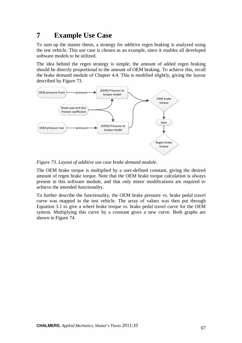
CHALMERS, Applied Mechanics, Master‟s Thesis 2011:10 67
7 Example Use Case
To sum up the master thesis, a strategy for additive regen braking is analyzed using
the test vehicle. This use case is chosen as an example, since it enables all developed
software models to be utilized.
The idea behind the regen strategy is simple; the amount of added regen braking
should be directly proportional to the amount of OEM braking. To achieve this, recall
the brake demand module of Chapter 4.4. This is modified slightly, giving the layout
described by Figure 73.
OEM pressure front
Brake pad and disc friction coefficient
(OEM) Pressure to torque model
OEM brake torque
OEM pressure rear pressure
(OEM) Pressure to torque model
pressure
Regen brake torque
Gain
Figure 73. Layout of additive use case brake demand module.
The OEM brake torque is multiplied by a user-defined constant, giving the desired
amount of regen brake torque. Note that the OEM brake torque calculation is always
present in this software module, and that only minor modifications are required to
achieve the intended functionality.
To further describe the functionality, the OEM brake pressure vs. brake pedal travel
curve was mapped in the test vehicle. The array of values was then put through
Equation 3.1 to give a wheel brake torque vs. brake pedal travel curve for the OEM
system. Multiplying this curve by a constant gives a new curve. Both graphs are
shown in Figure 74.
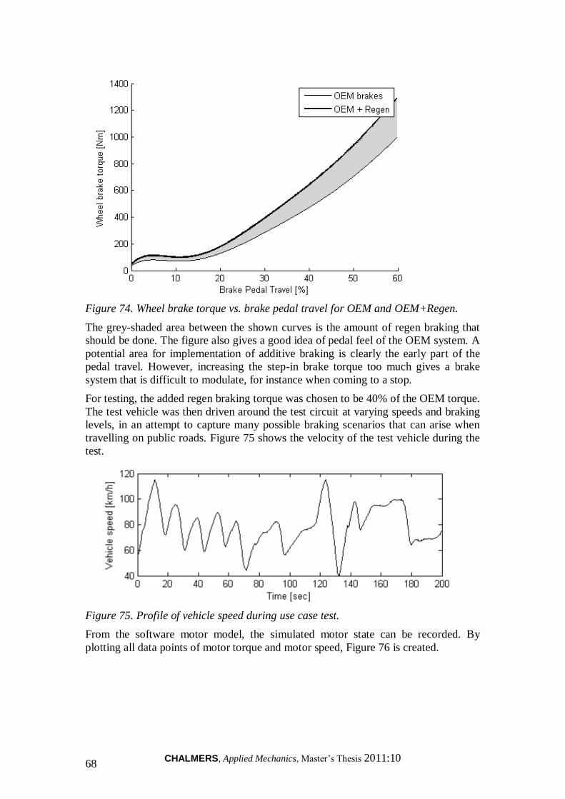
CHALMERS, Applied Mechanics, Master‟s Thesis 2011:10 68
Figure 74. Wheel brake torque vs. brake pedal travel for OEM and OEM+Regen.
The grey-shaded area between the shown curves is the amount of regen braking that
should be done. The figure also gives a good idea of pedal feel of the OEM system. A
potential area for implementation of additive braking is clearly the early part of the
pedal travel. However, increasing the step-in brake torque too much gives a brake
system that is difficult to modulate, for instance when coming to a stop.
For testing, the added regen braking torque was chosen to be 40% of the OEM torque.
The test vehicle was then driven around the test circuit at varying speeds and braking
levels, in an attempt to capture many possible braking scenarios that can arise when
travelling on public roads. Figure 75 shows the velocity of the test vehicle during the
test.
Figure 75. Profile of vehicle speed during use case test.
From the software motor model, the simulated motor state can be recorded. By
plotting all data points of motor torque and motor speed, Figure 76 is created.
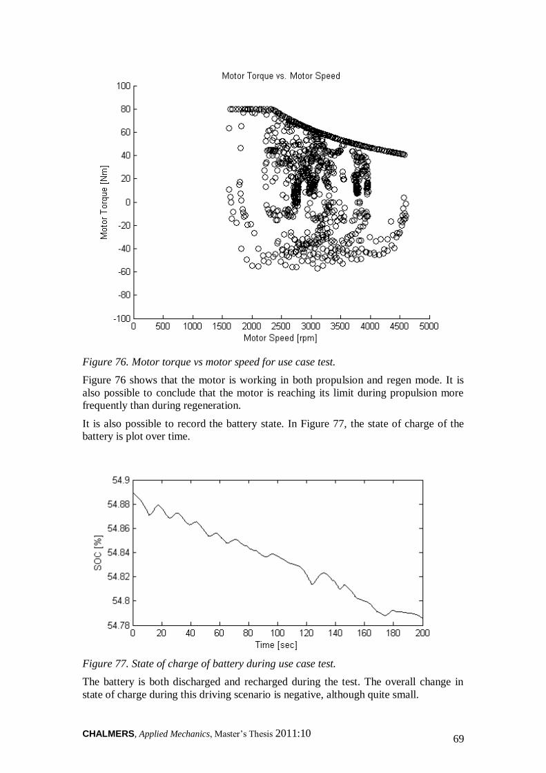
CHALMERS, Applied Mechanics, Master‟s Thesis 2011:10 69
Figure 76. Motor torque vs motor speed for use case test.
Figure 76 shows that the motor is working in both propulsion and regen mode. It is
also possible to conclude that the motor is reaching its limit during propulsion more
frequently than during regeneration.
It is also possible to record the battery state. In Figure 77, the state of charge of the
battery is plot over time.
Figure 77. State of charge of battery during use case test.
The battery is both discharged and recharged during the test. The overall change in
state of charge during this driving scenario is negative, although quite small.
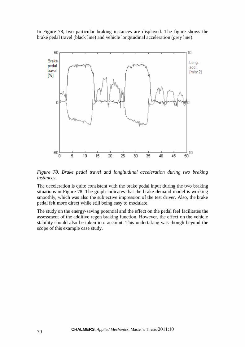
CHALMERS, Applied Mechanics, Master‟s Thesis 2011:10 70
In Figure 78, two particular braking instances are displayed. The figure shows the
brake pedal travel (black line) and vehicle longitudinal acceleration (grey line).
Figure 78. Brake pedal travel and longitudinal acceleration during two braking
instances.
The deceleration is quite consistent with the brake pedal input during the two braking
situations in Figure 78. The graph indicates that the brake demand model is working
smoothly, which was also the subjective impression of the test driver. Also, the brake
pedal felt more direct while still being easy to modulate.
The study on the energy-saving potential and the effect on the pedal feel facilitates the
assessment of the additive regen braking function. However, the effect on the vehicle
stability should also be taken into account. This undertaking was though beyond the
scope of this example case study.
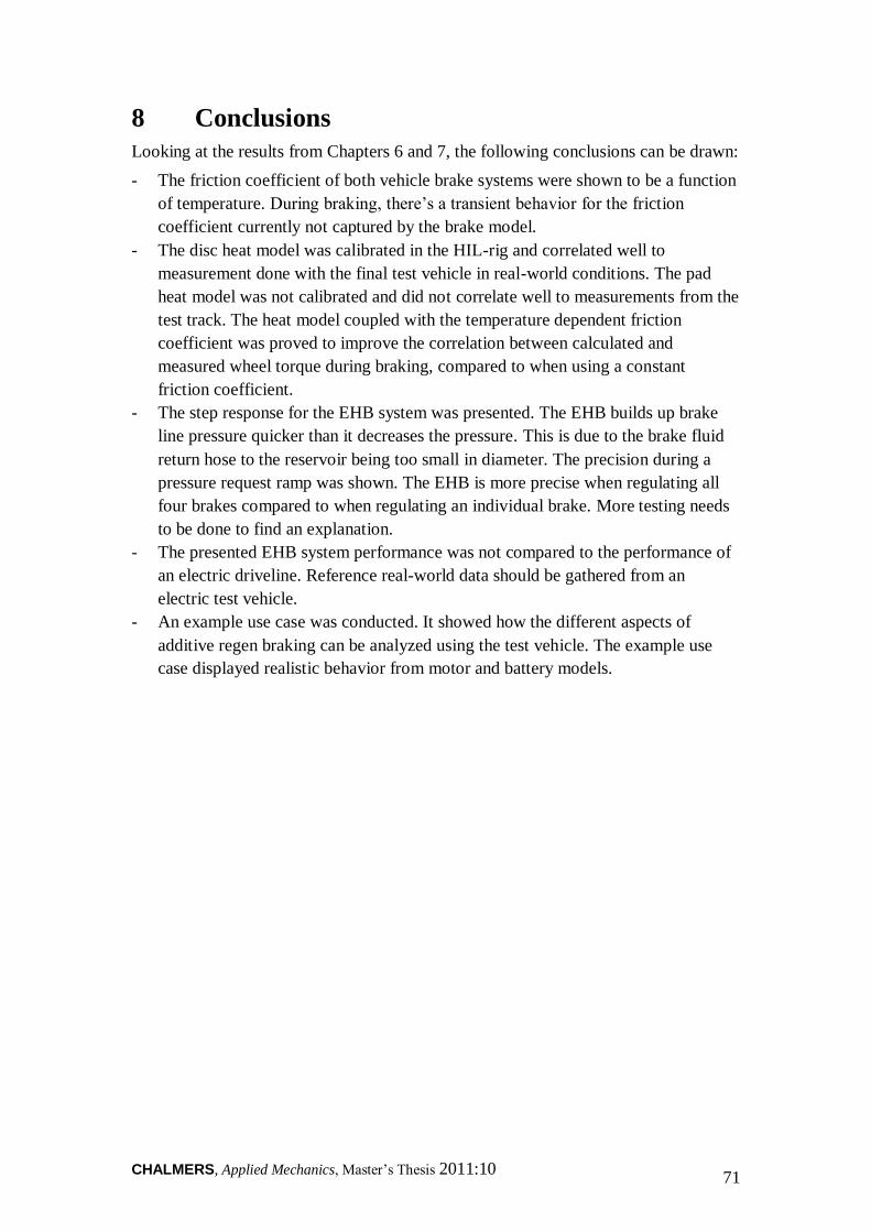
CHALMERS, Applied Mechanics, Master‟s Thesis 2011:10 71
8 Conclusions
Looking at the results from Chapters 6 and 7, the following conclusions can be drawn:
- The friction coefficient of both vehicle brake systems were shown to be a function
of temperature. During braking, there‟s a transient behavior for the friction
coefficient currently not captured by the brake model.
- The disc heat model was calibrated in the HIL-rig and correlated well to
measurement done with the final test vehicle in real-world conditions. The pad
heat model was not calibrated and did not correlate well to measurements from the
test track. The heat model coupled with the temperature dependent friction
coefficient was proved to improve the correlation between calculated and
measured wheel torque during braking, compared to when using a constant
friction coefficient.
- The step response for the EHB system was presented. The EHB builds up brake
line pressure quicker than it decreases the pressure. This is due to the brake fluid
return hose to the reservoir being too small in diameter. The precision during a
pressure request ramp was shown. The EHB is more precise when regulating all
four brakes compared to when regulating an individual brake. More testing needs
to be done to find an explanation.
- The presented EHB system performance was not compared to the performance of
an electric driveline. Reference real-world data should be gathered from an
electric test vehicle.
- An example use case was conducted. It showed how the different aspects of
additive regen braking can be analyzed using the test vehicle. The example use
case displayed realistic behavior from motor and battery models.

CHALMERS, Applied Mechanics, Master‟s Thesis 2011:10 72
CHALMERS, Applied Mechanics, Master‟s Thesis 2011:10 73
9 Future Work
To gain better EHB performance, further development of the brake heat model is
recommended. This necessitates the implementation of a thermocouple in the brake
HIL-rig to better understand the thermodynamic behavior of the brake pads. To make
data sampling in the test vehicle easier, thermocouples and IR-sensors can be installed
to monitor brake and disc temperatures respectively.
The friction coefficient variation over temperature of the rear EHB and OEM brakes
should be determined using the same procedure as the one used for the front axle. The
rear EHB system pads are the same as for the front, so they can be expected to behave
similarly to the front brakes. However, the rear OEM system pads are not the same
material as the front OEM pads, so they might display slightly different properties.
Future work naturally includes putting the test vehicle into use. That is to say, let
engineers apply their models in the vehicle. Running the test car will reveal more
attributes of the vehicle than shown in this study, such as long-term reliability,
flexibility of software and overall ease-of-use. At its current state, the car can very
well be used for basic function testing and clinic studies.
Reference testing of an electric vehicle should be conducted if knowledge of the
relative brake performance of the EHB system compared to an actual electric
driveline is vital. The brake response time of an electric vehicle can be measured
either monitoring its longitudinal acceleration or by using the torque wheels.
Using the experiences gained from the test sessions conducted, control functions of
the production cars can be developed. This may lead to more efficient, safe and
reliable embedded vehicle systems.

CHALMERS, Applied Mechanics, Master‟s Thesis 2011:10 74
CHALMERS, Applied Mechanics, Master‟s Thesis 2011:10 75
10 References
Andersson, M, et al. "Road Friction Estimation, IVSS Project Report." 2009.
BBC news. http://news.bbc.co.uk/2/hi/business/8497471.stm. February 2010.
Blundell, Michael and Damian Harty. Multibody Systems Approach To Vehicle
Dynamics. Elsevier Science & Technology, 2004.
Coelingh, Erik, Pascal Chaumette and Mats Andersson. "Open-Interface Definitions
for Automotive Systems Application to a Brake by Wire System." 2002.
Day, Andrew J, Hon Ping Ho and Khalid Hussain. "Brake System Simulation to
Predict Brake Pedal Feel in a Passenger Car." 2009.
de Arruda Pereira, Joaquim A. "New Fiesta: Brake Pedal Feeling Development to
Improve Customer Satisfaction." 2003.
Elert, Glenn. The Physics Hypertextbook. 1998. December 2010
<http://physics.info>.
Hancock, Matthew and Francis Assadian. "Impact of Regenerative Braking on
Vehicle Stability." 2007.
Hoffman, Lars. Electric Motor Drives Horace Ka Ho Lai and David Madås. 14
October 2010.
Hopkins, Brad, Saied Taheri and Mehdi Ahmadian. "Yaw Stability Control and
Emergency Roll Control for Vehicle Rollover Mitigation." 2010.
Hoseinnezhad, Reza and Alireza Bab-Hadiashar. "Recent Patents on Measurement
and Estimation in Brake-By-Wire." 2008.
Hughes, Austin. Electric Motors and Drives. Oxford: Elsevier Ltd., 2006.
IBT Power Ltd. Lithium Ion Technical Data. 2011. <http://www.ibt-
power.com/Battery_packs/Li_Ion/Lithium_ion_tech.html>.
Milliken, William F and Douglas L Milliken. Race Car Vehicle Dynamics. Milliken
Research Associates, 1995.
Olsson, Gunnar, et al. Use case definition meeting David Madås and Horace Lai.
December 2010.
Pascali, Leonardo, et al. "Customer Orientation: A Further Target in Brake System
Design." 2003.
Rajesh, A T, Bisen Badal and Sharad Pol. "Co-relating Subjective and Objective
Brake Performance: A Case Study." 2006.
Shim, Taehyun and Donald Margolis. "Using μ Feedforward for Vehicle Stability
Enhancement." n.d.
Talati, Faramarz and Salman Jalalifar. "Analysis of heat conduction in a disk brake
system." 2009.
Wicks, Frank and Kyle Donnelly. "Modeling Regenerative Braking and Storage for
Vehicles." 1999.
von Albrichsfeld, Christian and Jürgen Karner. "Brake System for Hybrid and Electric
Vehicles." 2009.

CHALMERS, Applied Mechanics, Master‟s Thesis 2011:10 76
![REGENERATIVE BRAKING SYSTEM IN ELECTRIC VEHICLES · REGENERATIVE BRAKING SYSTEM IN ELECTRIC VEHICLES ... REGENERATIVE BRAKING SYSTEM ... Regenerative action during braking[9]](https://img.pdfslide.net/doc/110x75/5adccef67f8b9a1a088c7cf0/regenerative-braking-system-in-electric-vehicles-braking-system-in-electric-vehicles.jpg)