Embed Size (px)
Citation preview
Université de ProvenceAix-Marseille I
Christian Marinoni
Testing gravity and cosmological models at z~1
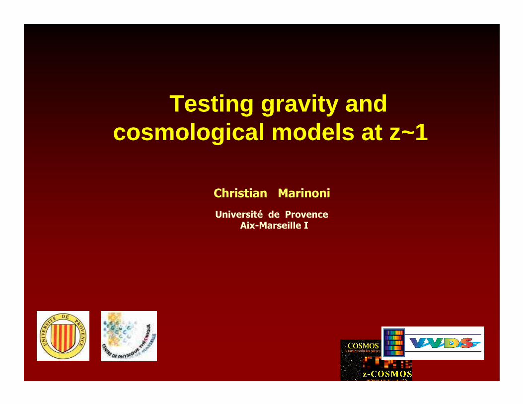
Un unprecedented convergence of results in cosmology over the last few years are interpreted as follows
- ordinary matter is a minority (1/6) of all matter- matter is a minority (1/4) of all energy- geometry is spatially flat - expansion is presently accelerated
accelerating
decelerating
State of the Art
parameters precision Vs.
hypotheses precision
Modified gravity is not particularly attractive theoretically, but the observed cosmic acceleration is so surprising that all plausibleexplanations should be considered.
Standard ΛCDM model!
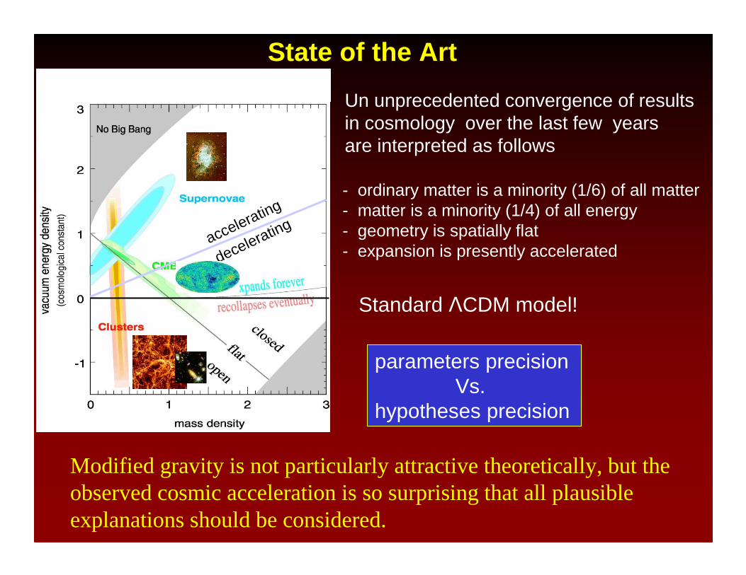
Eratosthène et son modèle de la Terre (~ 220 av. JC)
Hypothèses : -La terre est ronde et les deux villes sont sur le même cercle maxime (méridien)
- le soleil était très éloignéde la Terre, de telle sorte que ses rayons arrivaientparallèlement entre eux
- Le jour du solstice d'été, à midi, le Soleil était au zénith à Syene et les objets n'avaient pas d'ombre
- Le même jours, a la même heure, les rayons du Soleil, faisaient un angle de 7°avec la verticale à Alexandrie
Observations :
Conclusions :rayon de la terre déterminéavec une précision de 3%
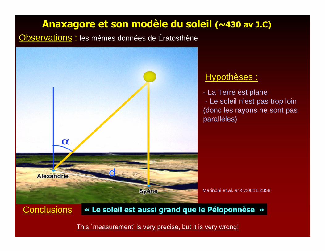
Anaxagore et son modèle du soleil (~430 av J.C)
Observations : les mêmes données de Ératosthène
Hypothèses :
« Le soleil est aussi grand que le Péloponnèse »Conclusions
- La Terre est plane- Le soleil n’est pas trop loin
(donc les rayons ne sont pas parallèles)
This `measurement’ is very precise, but it is very wrong!
Marinoni et al. arXiv:0811.2358
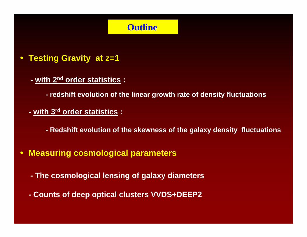
• Testing Gravity at z=1
- with 2nd order statistics :
- redshift evolution of the linear growth rate of density fluctuations
- with 3rd order statistics :
- Redshift evolution of the skewness of the galaxy density fluctuations
• Measuring cosmological parameters
- The cosmological lensing of galaxy diameters
- Counts of deep optical clusters VVDS+DEEP2
Outline
πGρδ4H
0
−=+∂∂
=+∂∂
θτθ
θτδ
vx ⋅∇≡
−=
θρ
ρρδ
ttGa δρπτδ
τδ 2
2
2
4H =∂∂+
∂∂
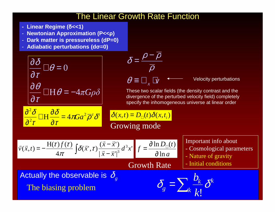
- Linear Regime ( δ<<1)- Newtonian Approximation (P<< ρ)- Dark matter is pressureless (dP=0)- Adiabatic perturbations (d σ=0)
The Linear Growth Rate Function
Velocity perturbations
These two scalar fields (the density contrast and the divergence of the perturbed velocity field) completely specify the inhomogeneous universe at linear order
∫ −−−= '
|'|
)'(),'(
4
)()H(),( 3
3xd
xx
xxx
ftxv vr
rrrrr τδ
πττ
),()(),( itxtDtx δδ +=Growing mode
a
tDf
ln
)(ln
∂∂= +
Growth Rate
Important info about- Cosmological parameters- Nature of gravity- Initial conditions
∑=k
kkg k
b δδ!
Actually the observable is gδThe biasing problem
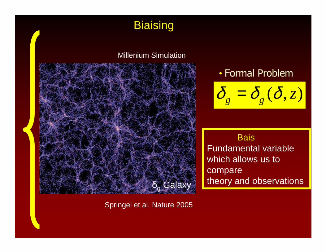
Biaising
δ Matter δg Galaxy
Springel et al. Nature 2005
Millenium Simulation
),( zgg δδδ =• Formal Problem
BaisFundamental variablewhich allows us to comparetheory and observations
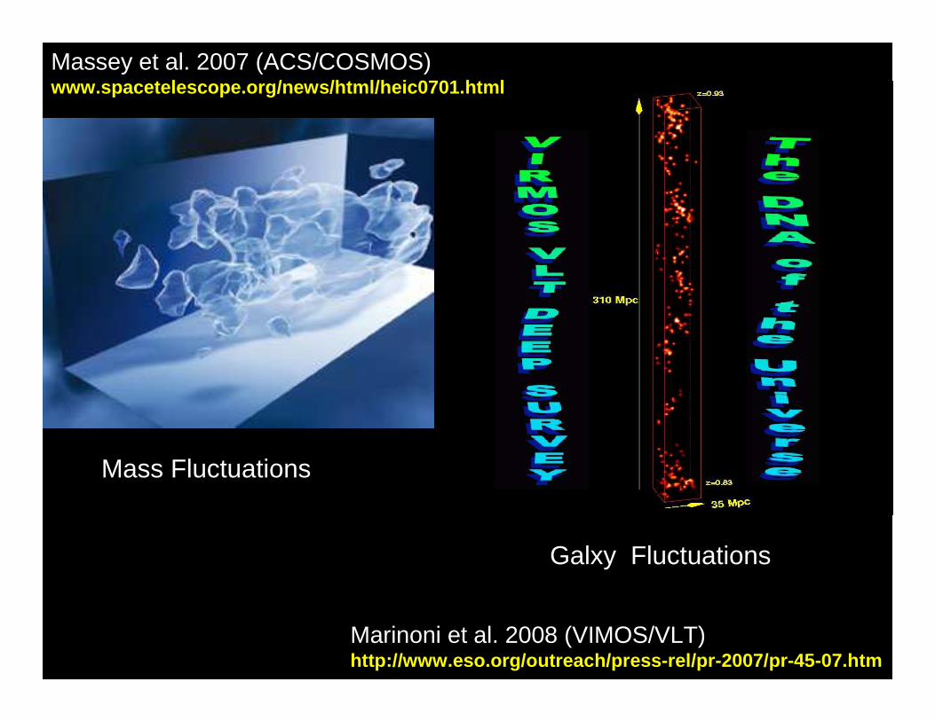
Massey et al. 2007 (ACS/COSMOS)www.spacetelescope.org/news/html/heic0701.html
Marinoni et al. 2008 (VIMOS/VLT)http://www.eso.org/outreach/press-rel/pr-2007/pr-45 -07.htm
Mass Fluctuations
Galxy Fluctuations
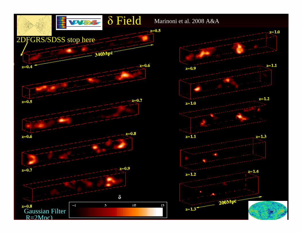
δ Field
2DFGRS/SDSS stop here
Marinoni et al. 2008 A&A
Gaussian FilterR=2Mpc)
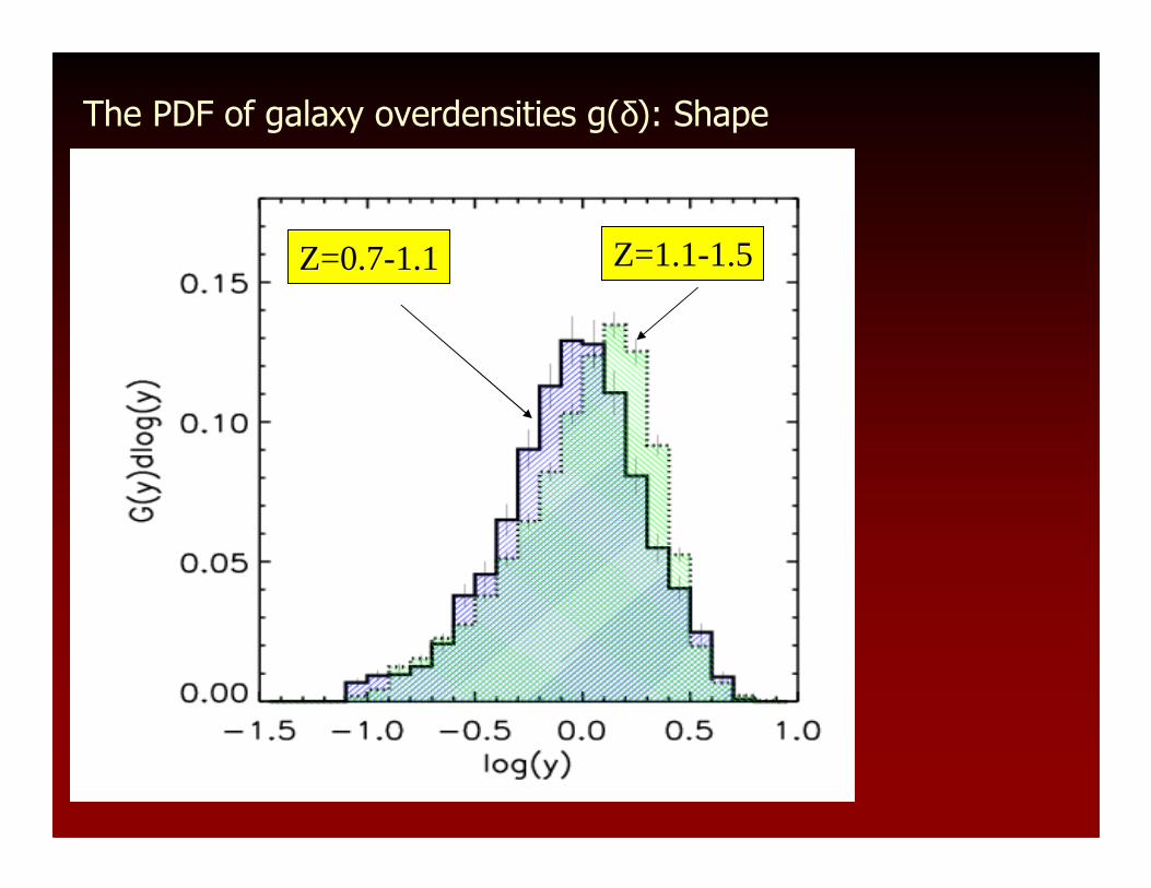
The PDF of galaxy overdensities g(δ): Shape
Z=0.7-1.1 Z=1.1-1.5
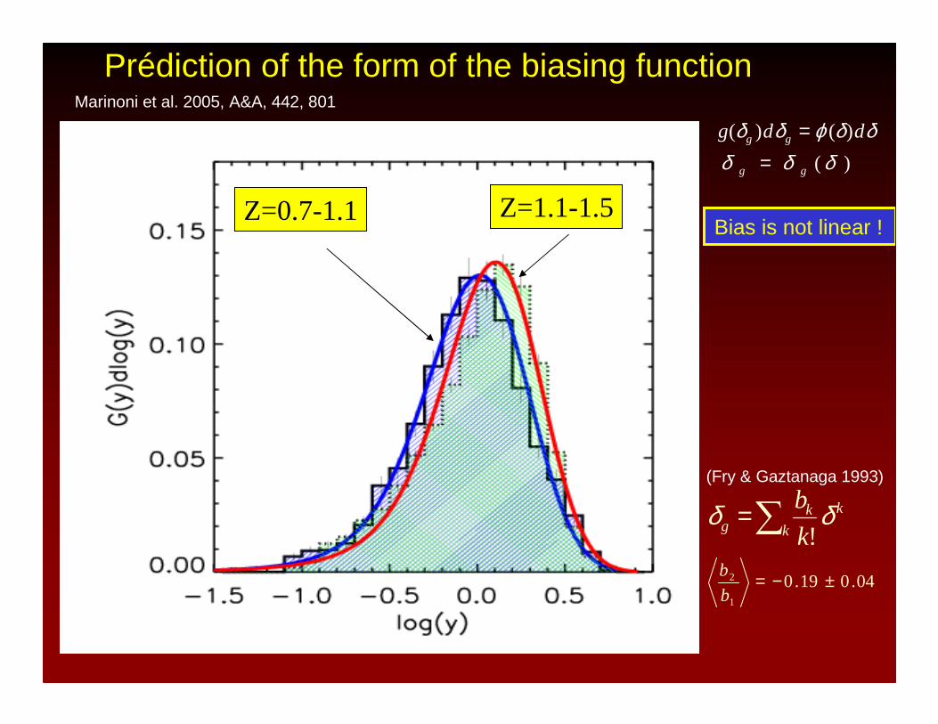
Z=0.7-1.1 Z=1.1-1.5
g(δg )dδg = ϕ (δ)dδ
Prédiction of the form of the biasing function
)(δδδ gg =
Bias is not linear !
Marinoni et al. 2005, A&A, 442, 801
04.019.01
2 ±−=b
b
∑=k
kkg k
b δδ!
(Fry & Gaztanaga 1993)
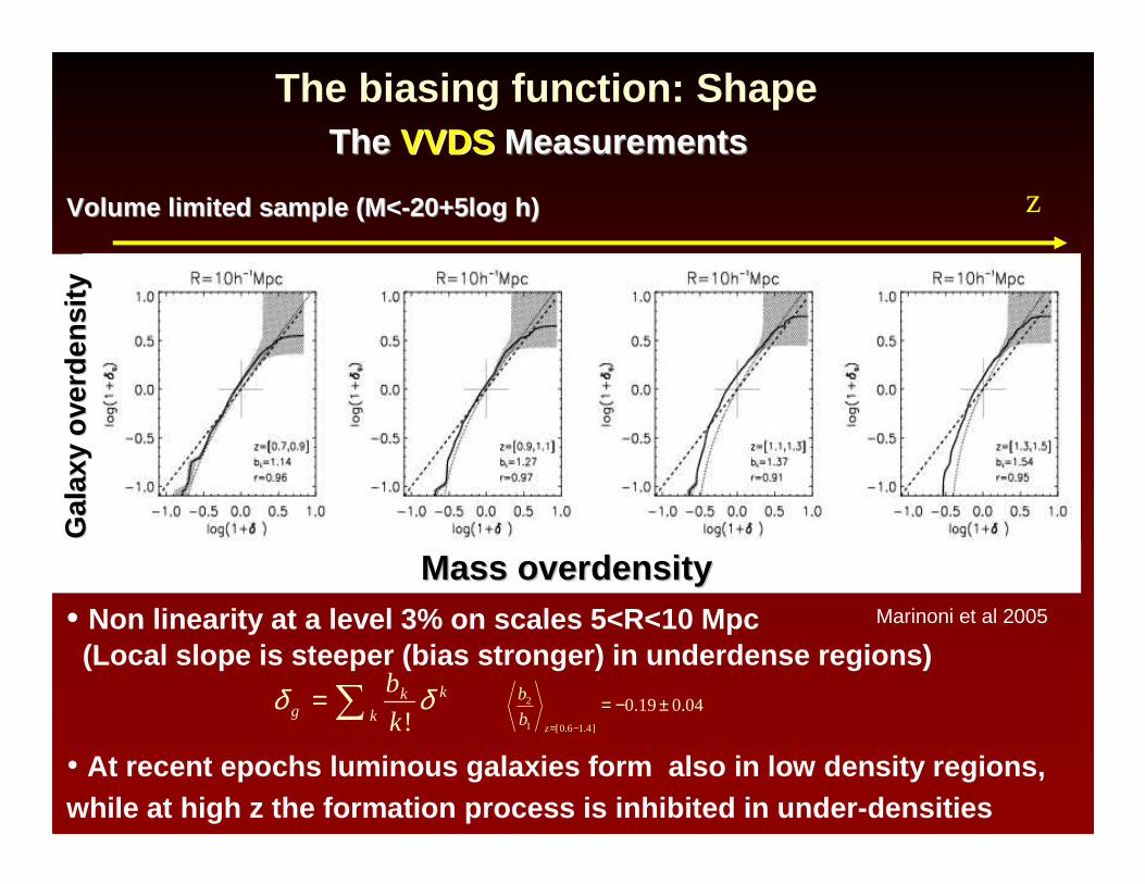
The biasing function: Shape
z
• At recent epochs luminous galaxies form also in lo w density regions, while at high z the formation process is inhibited in under-densities
The The VVDSVVDS MeasurementsMeasurements
• Non linearity at a level 3% on scales 5<R<10 Mpc(Local slope is steeper (bias stronger) in underden se regions)
Gal
axy
Gal
axy
over
dens
ityov
erde
nsity
Mass Mass overdensityoverdensity
Volume Volume limited sample limited sample (M<(M<--20+5log h)20+5log h)
04.019.0]4.16.0[1
2 ±−=−=z
b
b∑=k
kkg k
b δδ!
Marinoni et al 2005
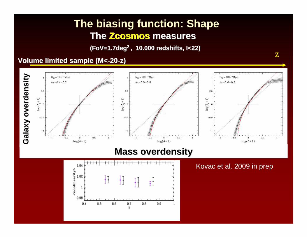
The biasing function: Shape
z
The The ZcosmosZcosmos measuresmeasures((FoVFoV=1.7deg=1.7deg 2 2 , 10.000 , 10.000 redshiftsredshifts , I<22), I<22)
Gal
axy
Gal
axy
over
dens
ityov
erde
nsity
Mass Mass overdensityoverdensity
Volume Volume limited sample limited sample (M<(M<--2020--z)z)
04.019.01
2 ±−=b
b
Kovac et al. 2009 in prep
There are several observational approaches that can lead to the determination of f(z).
- Redshift distortions of galaxy clustering (ξ(r), P(k) )- The rms mass fluctuation σ8(z) from galaxy and Ly −surveys - Weak lensing statistics, - Xray luminous galaxy clusters, - Integrated Sachs-Wolfe (ISW) effect.
Unfortunately, the currently available data are limited in number and accuracy and come mainly from the first two categories
- Redshift distortions of galaxy clustering (ξ(r), P(k) )- The rms mass fluctuation σ8(z) from galaxy and Ly −surveys- Weak lensing statistics, - Xray/Optical galaxy clusters, - Integrated Sachs-Wolfe (ISW) effect.
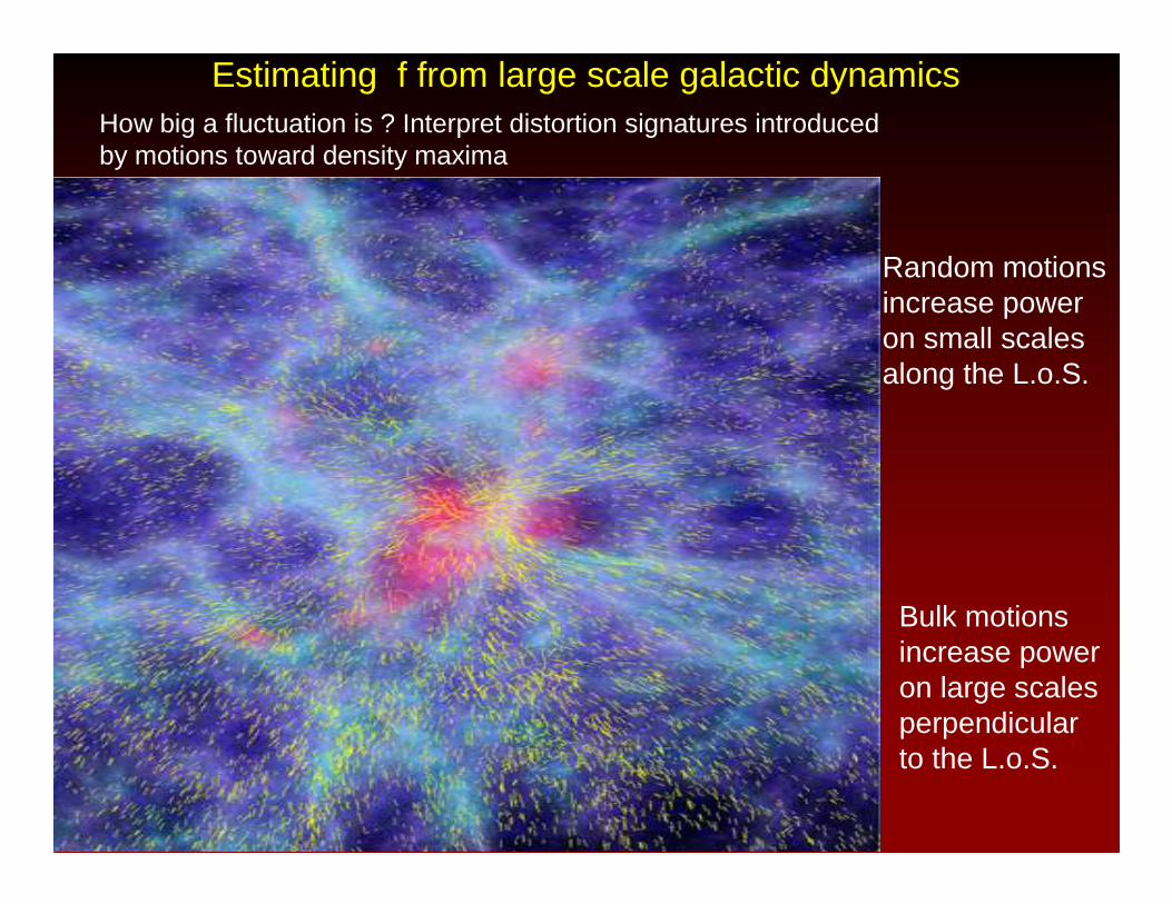
Bulk motions increase poweron large scalesperpendicularto the L.o.S.
Real Space
Z-Space Random motions increase poweron small scalesalong the L.o.S.
Redshift Space
SmallScales
LargeScales
Estimating f from large scale galactic dynamicsHow big a fluctuation is ? Interpret distortion signatures introducedby motions toward density maxima
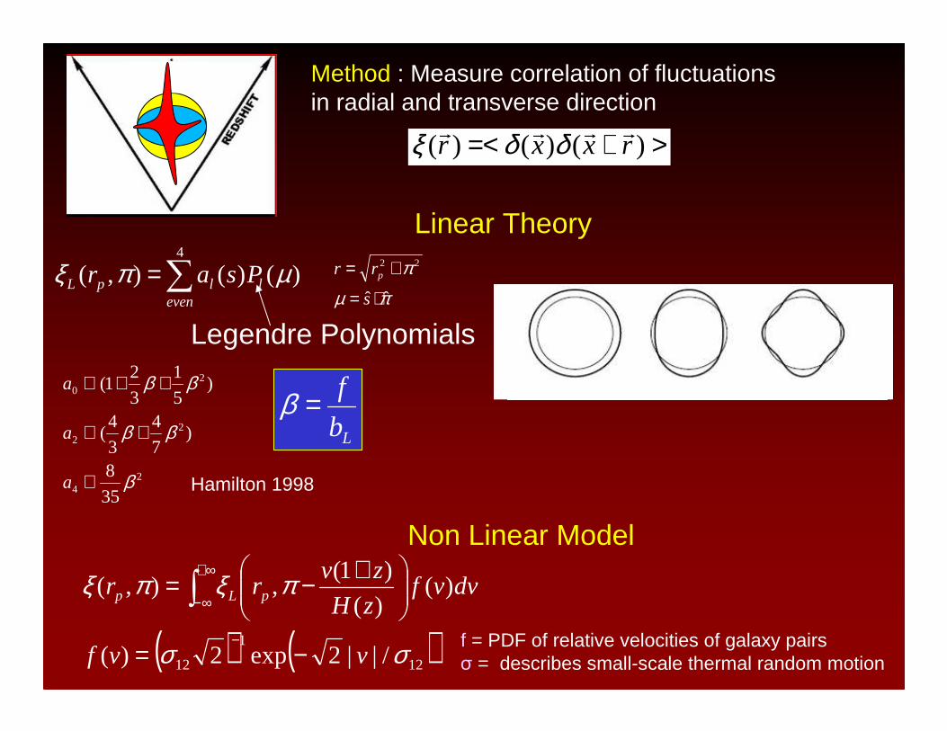
>+=< )()()( rxxrrrrr δδξ
Non Linear Model
( ) ( )12
1
12 /||2exp2)(
)()(
)1(,),(
σσ
πξπξ
vvf
dvvfzH
zvrr pLp
−=
+−=
−
∞+
∞−∫f = PDF of relative velocities of galaxy pairsσ = describes small-scale thermal random motion
24
22
20
35
8
)7
4
3
4(
)5
1
3
21(
β
ββ
ββ
∝
+∝
++∝
a
a
a
πµ
πˆˆ
22
⋅=
+=
s
rr p
Legendre Polynomials
Linear Theory
∑=4
)()(),(even
llpL Psar µπξ
Lb
f=β
Hamilton 1998
Method : Measure correlation of fluctuations in radial and transverse direction
2dFGRS <Z>=0.1250,000 galaxiesf=0.5±0.1σ=390±50 km/s
(Peacock et al. 2001, Nature)
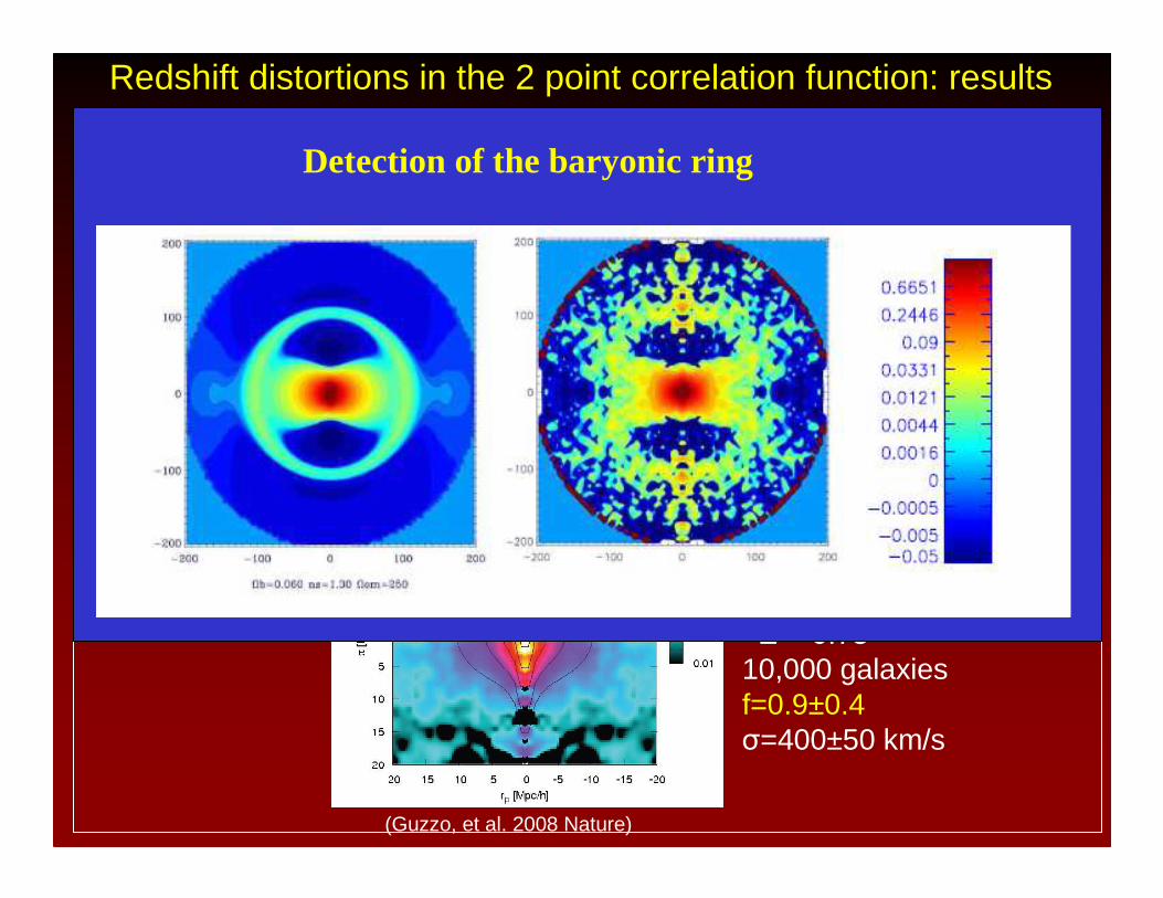
Redshift distortions in the 2 point correlation function: results
VVDS
<Z>=0.7510,000 galaxiesf=0.9±0.4σ=400±50 km/s
(Guzzo, et al. 2008 Nature)
SDSS <Z>=0.3475,000 LRGf=0.64±0.09σ=392±30 km/s
(Cabre & Gaztanaga 2009, MNRAS)
Detection of the baryonic ring
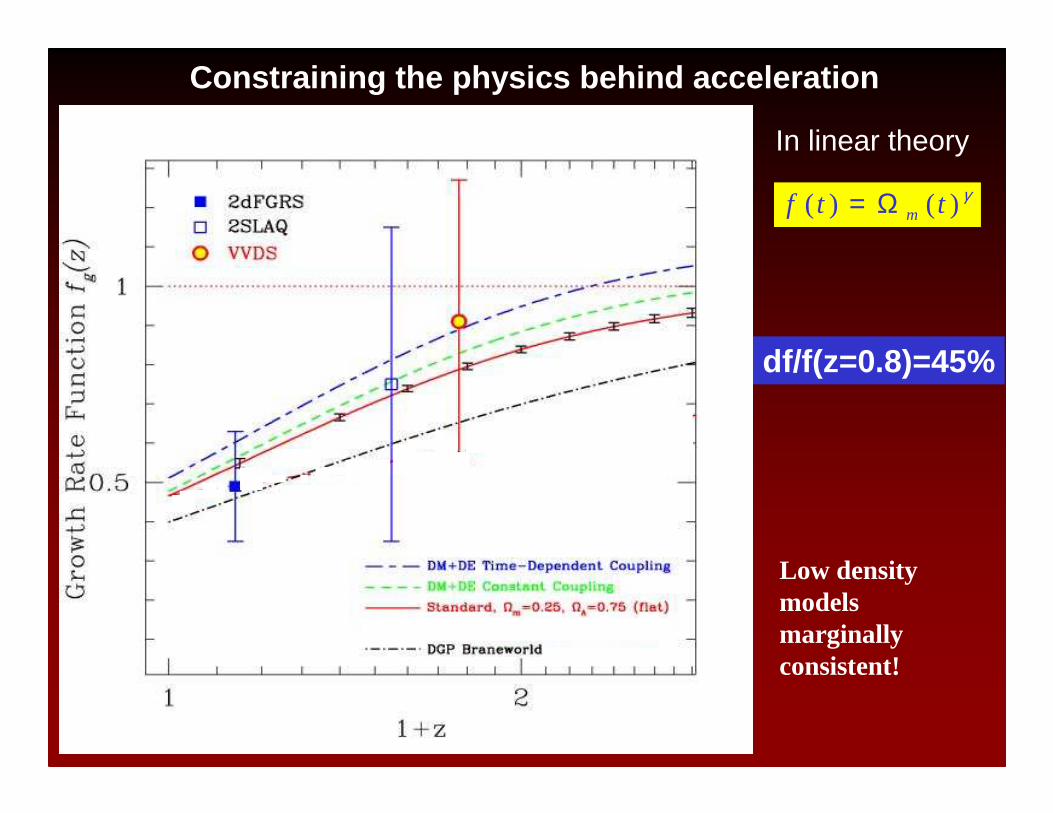
Constraining the physics behind acceleration
df/f(z=0.8)=45%
γ)()( ttf mΩ=
In linear theory
Low density modelsmarginallyconsistent!
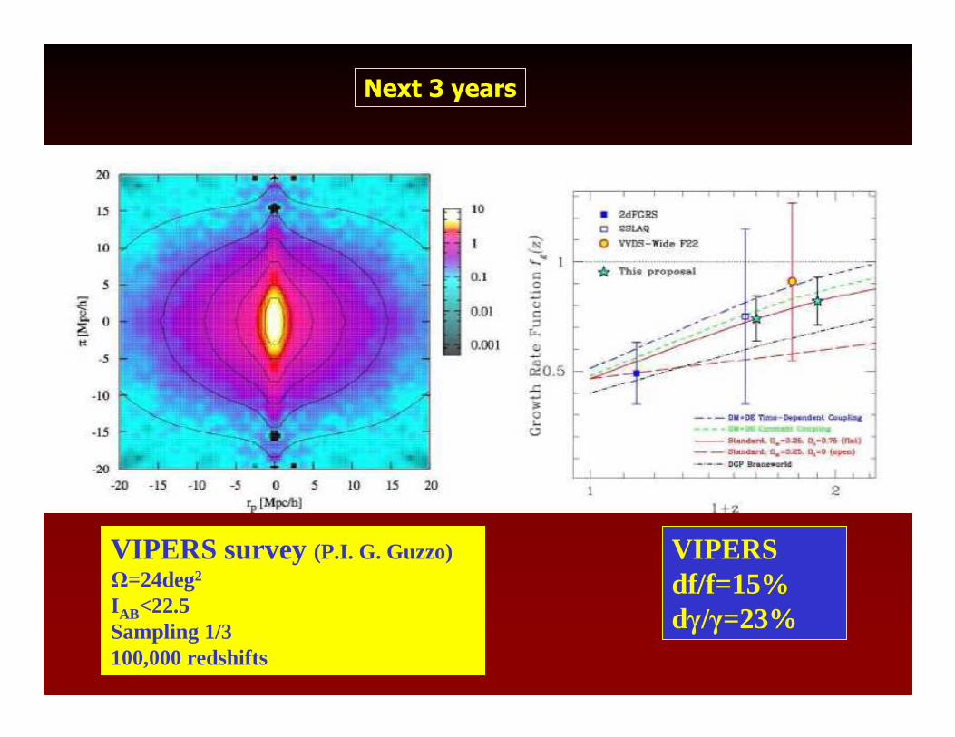
Next 3 years
VIPERSdf/f=15%dγ/γ=23%
VIPERS survey (P.I. G. Guzzo)Ω=24deg2
IAB<22.5Sampling 1/3100,000 redshifts

Euclidedf/f=1%dγ/γ=1.5%
Next 10 years
....if you know the bias to 1%
VIPERS EuclideΩ=2π srH<22Sampling 1/31.6 108 galaxies
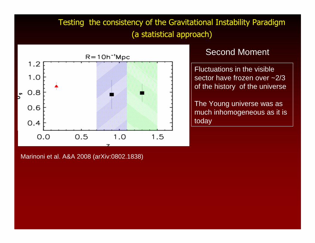
Testing the consistency of the Gravitational Instability Paradigm
(a statistical approach)
Fluctuations in the visible sector have frozen over ~2/3 of the history of the universe
The Young universe was as much inhomogeneous as it is today
Marinoni et al. A&A 2008 (arXiv:0802.1838)
Second Moment
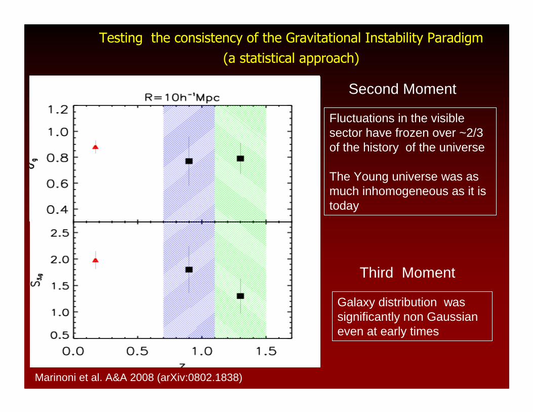
Testing the consistency of the Gravitational Instability Paradigm
(a statistical approach)
Marinoni et al. A&A 2005
Fluctuations in the visible sector have frozen over ~2/3 of the history of the universe
The Young universe was as much inhomogeneous as it is today
Second Moment
Galaxy distribution was significantly non Gaussian even at early times
Third Moment
Marinoni et al. A&A 2008 (arXiv:0802.1838)
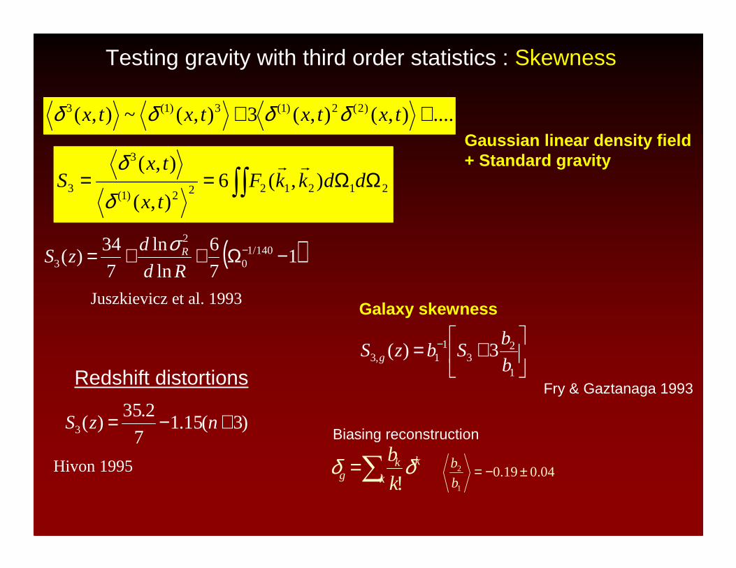
Testing gravity with third order statistics : Skewness
04.019.01
2 ±−=b
b∑=k
kkg k
b δδ!
Biasing reconstruction
R=10h-1Mpc
Juszkievicz et al. 1993
( )17
6
ln
ln
7
34)( 140/1
0
2
3 −Ω++= −
Rd
dzS Rσ
Gaussian linear density field+ Standard gravity
∫∫ ΩΩ== 2121222)1(
3
3 ),(6),(
),(ddkkF
tx
txS
rr
δ
δ
....),(),(3),(~),( )2(2)1(3)1(3 ++ txtxtxtx δδδδ
+= −
1
23
11,3 3)(
b
bSbzS g
Galaxy skewness
Hivon 1995
)3(15.17
2.35)(3 +−= nzS
Redshift distortionsFry & Gaztanaga 1993
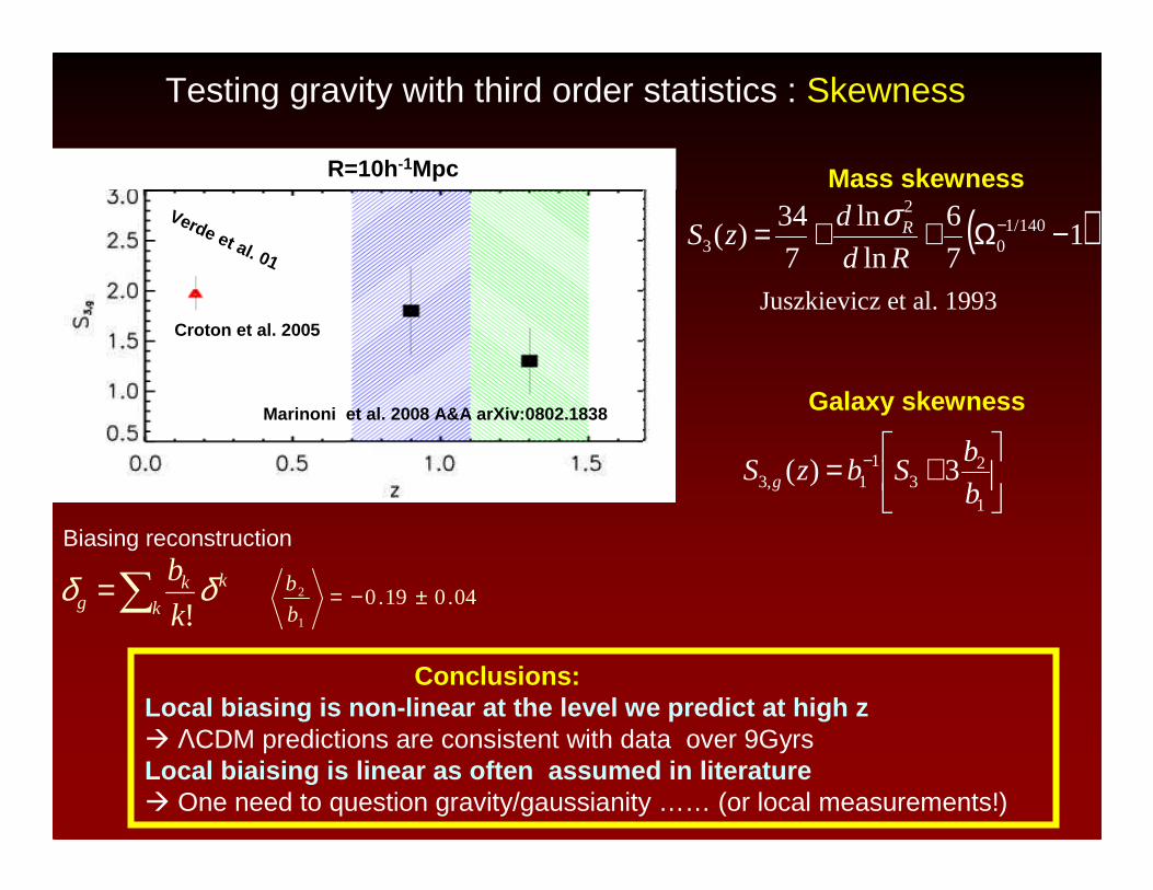
Testing gravity with third order statistics : Skewness
04.019.01
2 ±−=b
b∑=k
kkg k
b δδ!
Biasing reconstruction
R=10h-1Mpc
Marinoni et al. 2008 A&A arXiv:0802.1838
Verde et al. 01
Croton et al. 2005
Juszkievicz et al. 1993
( )17
6
ln
ln
7
34)( 140/1
0
2
3 −Ω++= −
Rd
dzS Rσ
+= −
1
23
11,3 3)(
b
bSbzS g
Mass skewness
Galaxy skewness
Conclusions:Local biasing is non-linear at the level we predict at high z ΛCDM predictions are consistent with data over 9GyrsLocal biaising is linear as often assumed in literature One need to question gravity/gaussianity …… (or local measurements!)
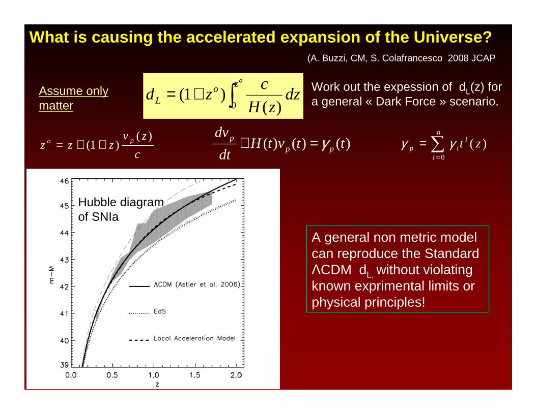
What is causing the accelerated expansion of the Univer se?
Assume onlymatter
Work out the expession of dL(z) for a general « Dark Force » scenario.∫+=
ozoL dz
zH
czd
0 )()1(
c
zvzzz po )()1( ++= ∑
=
=n
i
iip zt
0
)(γγ
A general non metric model can reproduce the Standard ΛCDM dL, without violating known exprimental limits or physical principles!
Hubble diagramof SNIa
)()()( ttvtHdt
dvpp
p γ=+
(A. Buzzi, CM, S. Colafrancesco 2008 JCAP
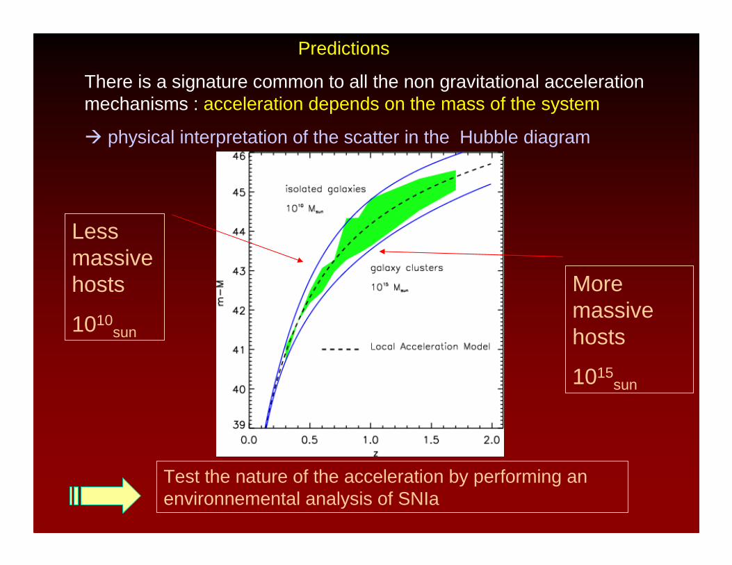
Test the nature of the acceleration by performing an environnemental analysis of SNIa
Lessmassive hosts
1010sun
More massive hosts
1015sun
Predictions
There is a signature common to all the non gravitational accelerationmechanisms : acceleration depends on the mass of the system
physical interpretation of the scatter in the Hubble diagram
• Testing Gravity at z=1
- with 2nd order statistics :
- redshift evolution of the linear growth factor of density fluctuations
- with 3rd order statistics :
- Redshift evolution of the skewness of the galaxy density fluctuations
• Testing cosmological models
- The cosmological lensing of galaxy diameters
- Counts of deep optical clusters VVDS+DEEP2
Outline
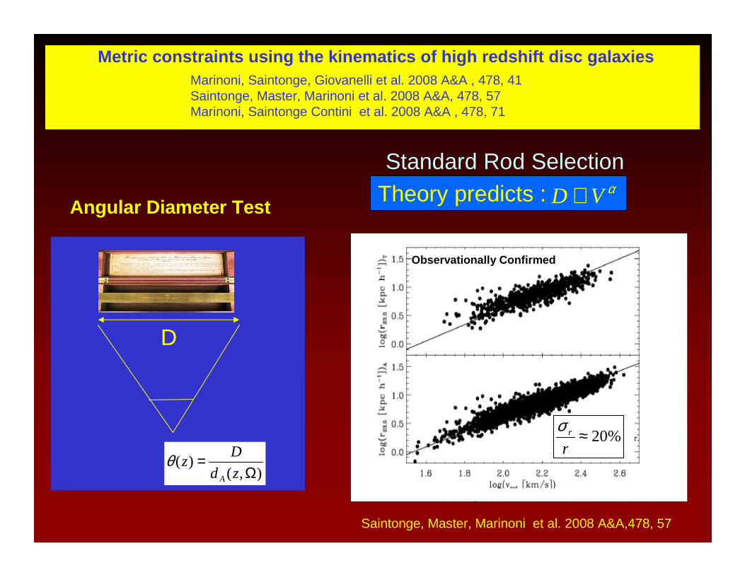
D
Angular Diameter Test
Metric constraints using the kinematics of high redshift disc galaxiesMarinoni, Saintonge, Giovanelli et al. 2008 A&A , 478, 41Saintonge, Master, Marinoni et al. 2008 A&A, 478, 57Marinoni, Saintonge Contini et al. 2008 A&A , 478, 71
),()(
Ω=
zd
Dz
A
θ
Theory predicts :Standard Rod Selection
Saintonge, Master, Marinoni et al. 2008 A&A,478, 57
Observationally Confirmed
%20≈r
rσ
αVD ∝
Z=0.5
Z=0.9
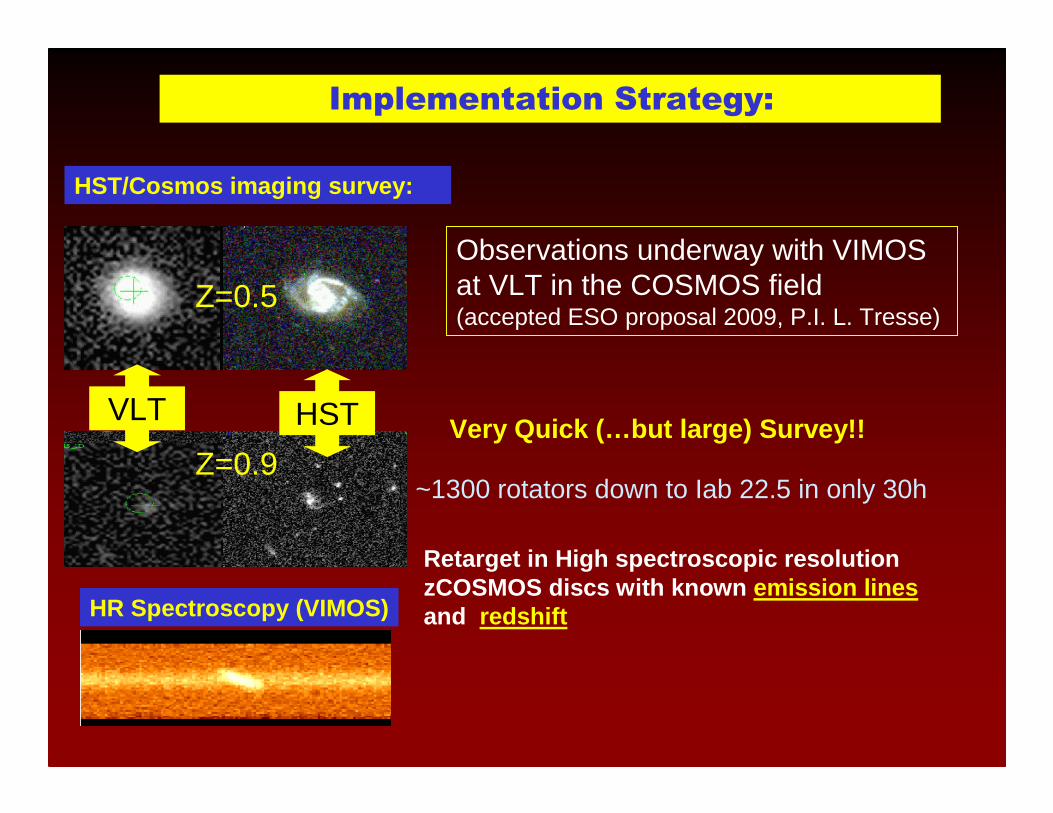
Implementation Strategy:
HST/Cosmos imaging survey:
HR Spectroscopy (VIMOS)
VLT HST
Observations underway with VIMOS at VLT in the COSMOS field(accepted ESO proposal 2009, P.I. L. Tresse)
Very Quick (…but large) Survey!!
~1300 rotators down to Iab 22.5 in only 30h
Retarget in High spectroscopic resolutionzCOSMOS discs with known emission linesand redshift

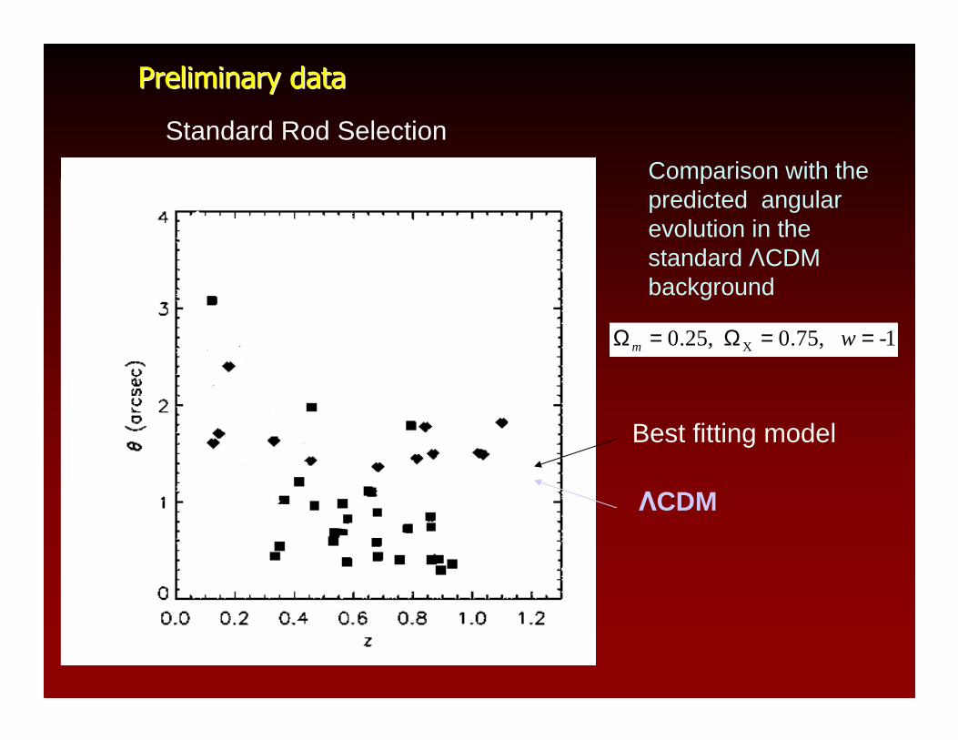
PreliminaryPreliminary datadata
1 ,75.0 ,25.0 X -wm ==Ω=Ω
Comparison with thepredicted angularevolution in the standard ΛCDM background
0<v(km/s)<100 100<v(km/s)<200
Standard Rod Selection
Best fitting model
ΛCDM
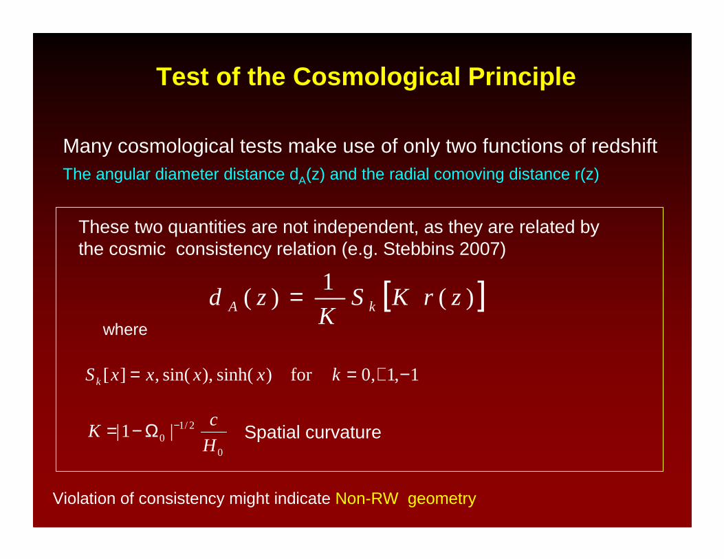
Many cosmological tests make use of only two functions of redshiftThe angular diameter distance dA(z) and the radial comoving distance r(z)
Violation of consistency might indicate Non-RW geometry
Test of the Cosmological Principle
These two quantities are not independent, as they are related by the cosmic consistency relation (e.g. Stebbins 2007)
[ ])( 1
)( zrKSK
zd kA =where
1,1,0for )sinh( ),sin( ,][ −+== kxxxxS k
0
2/10 |1|
H
cK −Ω−= Spatial curvature
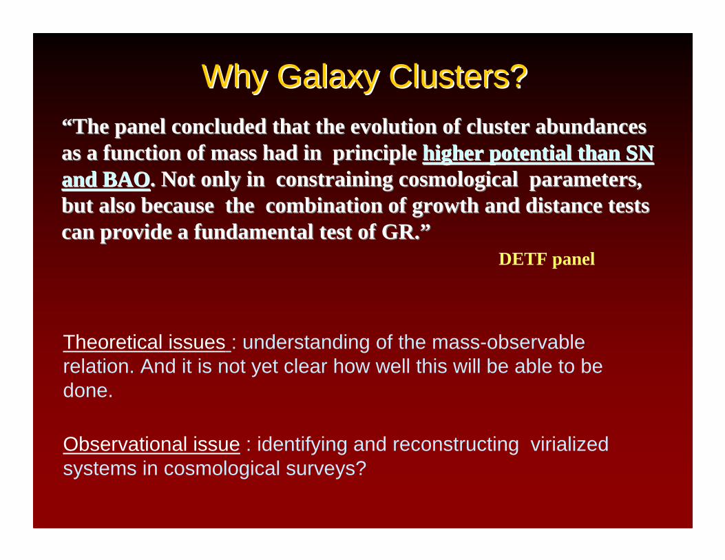
Why Galaxy Clusters?Why Galaxy Clusters?““ The panel concluded that the evolution of cluster abundances The panel concluded that the evolution of cluster abundances as a function of mass had in principle as a function of mass had in principle higher potential than SN higher potential than SN and BAOand BAO. Not only in constraining cosmological parameters, . Not only in constraining cosmological parameters, but also because the combination of growth and distance testsbut also because the combination of growth and distance testscan provide a fundamental test of GR.can provide a fundamental test of GR.””
DETF panel
Observational issue : identifying and reconstructing virializedsystems in cosmological surveys?
Theoretical issues : understanding of the mass-observable relation. And it is not yet clear how well this will be able to be done.
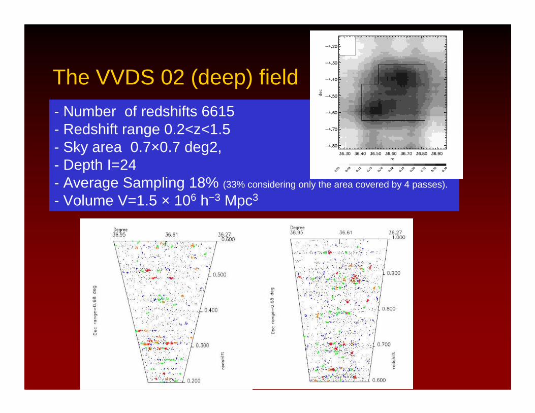
The VVDS 02 (deep) field
- Number of redshifts 6615- Redshift range 0.2<z<1.5- Sky area 0.7×0.7 deg2,- Depth I=24- Average Sampling 18% (33% considering only the area covered by 4 passes).
- Volume V=1.5 × 10⁶ h−3 Mpc3
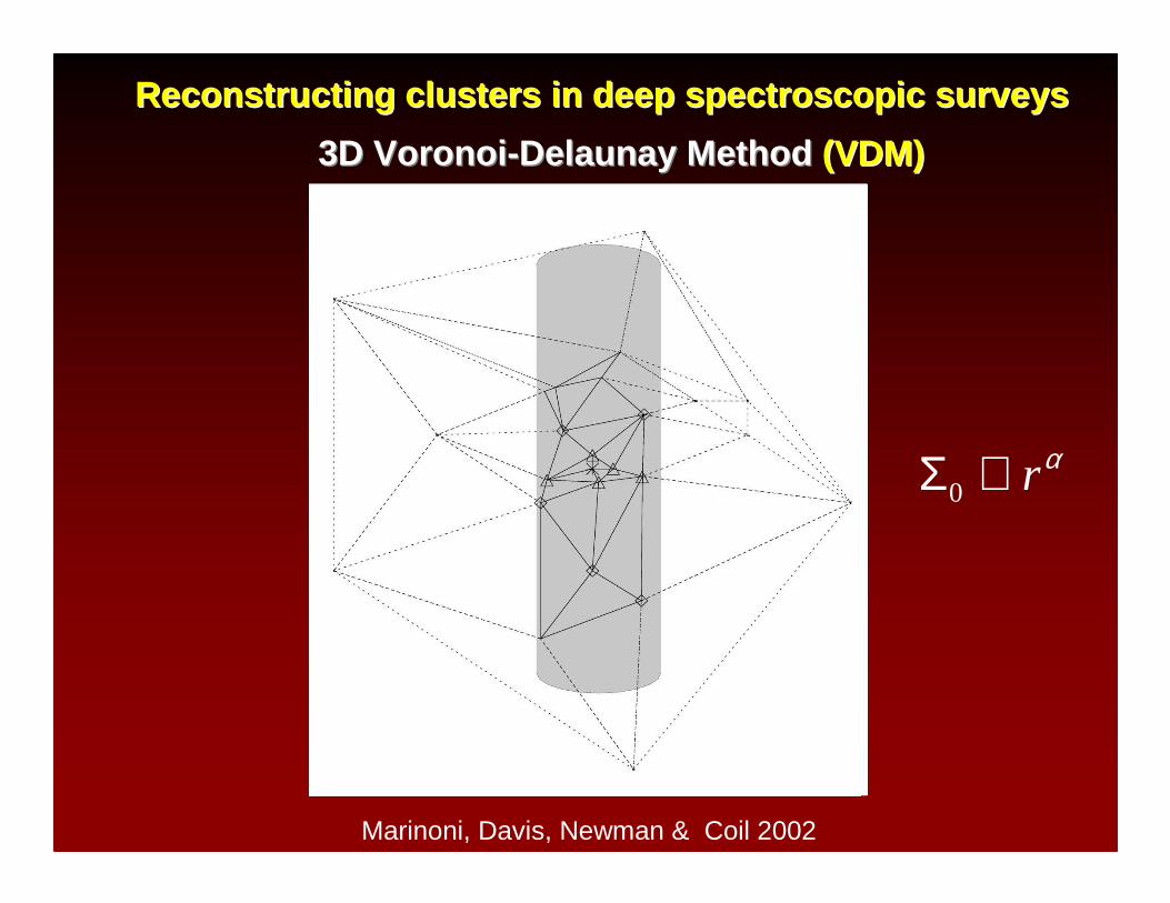
Reconstructing clusters in deep spectroscopic surve ysReconstructing clusters in deep spectroscopic surve ys
3D 3D VoronoiVoronoi --Delaunay Method Delaunay Method (VDM)(VDM)
Marinoni, Davis, Newman & Coil 2002
αr∝Σ0
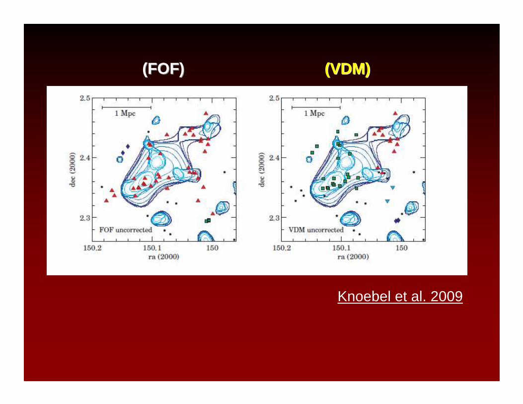
(FOF) (FOF) (VDM)(VDM)
Knoebel et al. 2009
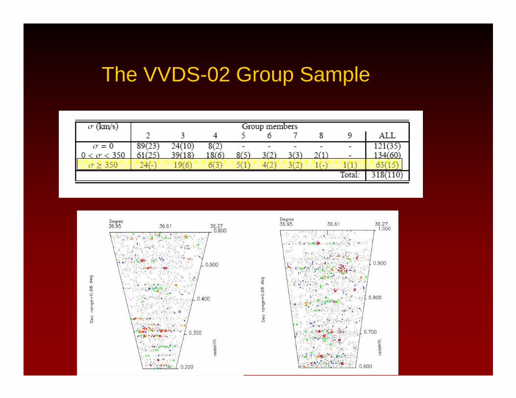
The VVDS-02 Group Sample
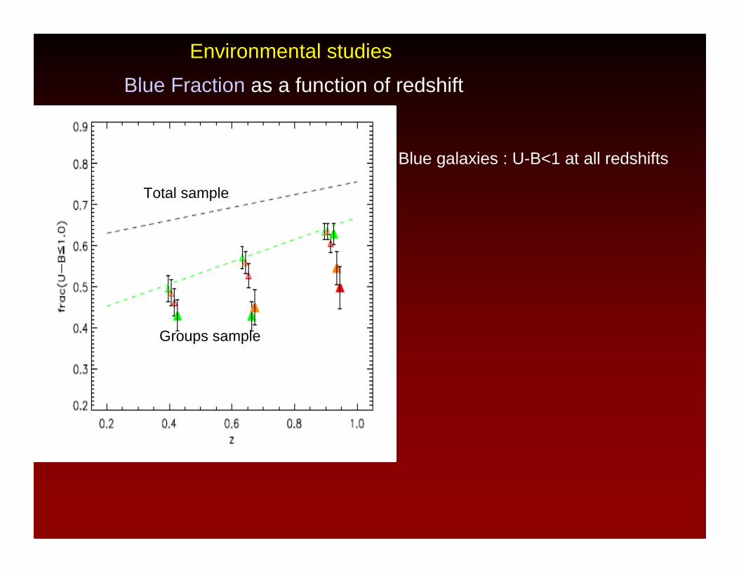
Blue Fraction as a function of redshift
Blue galaxies : U-B<1 at all redshifts
Environmental studies
Total sample
Groups sample
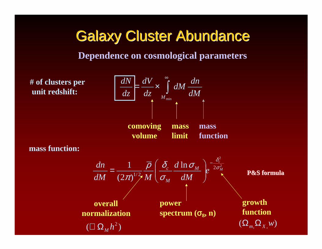
Galaxy Cluster AbundanceGalaxy Cluster AbundanceDependence on cosmological parameters
2
2
22/1
ln
)2(
1M
c
edM
d
MdM
dn M
M
c σδ
σσδρ
π
−
=
growthfunction
powerspectrum (σσσσ8, n)
P&S formulaP&S formula
∫∞
×=minM dM
dndM
dz
dV
dz
dN
comovingvolume
masslimit
massfunction
# of clusters perunit redshift:
mass function:
overallnormalization
)( 2hMΩ∝ )( ,, wXm ΩΩ
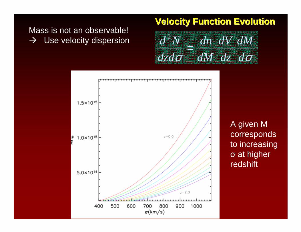
VelocityVelocity FunctionFunction EvolutionEvolution
σσ d
dM
dz
dV
dM
dn
dzd
Nd =2
Mass is not an observable! Use velocity dispersion
A given Mcorrespondsto increasingσ at higher redshift
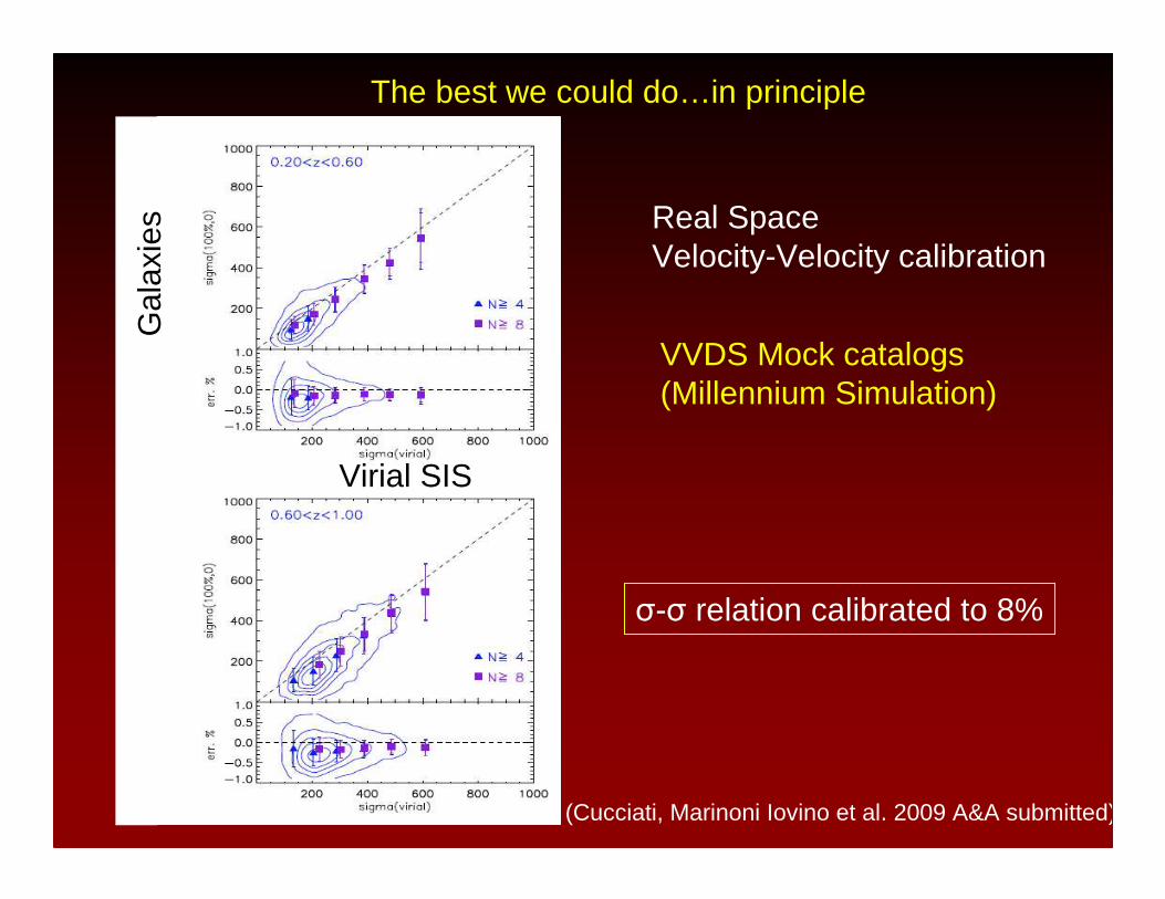
VVDS Mock catalogs (Millennium Simulation)
(Cucciati, Marinoni Iovino et al. 2009 A&A submitted)
Real SpaceVelocity-Velocity calibration
Gal
axie
s
σ-σ relation calibrated to 8%
Virial SIS
The best we could do…in principle
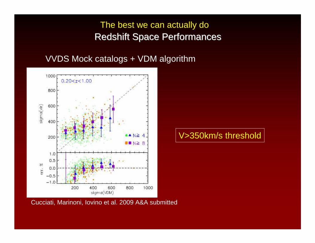
Redshift Redshift SpaceSpace Performances Performances
VVDS Mock catalogs + VDM algorithm
Cucciati, Marinoni, Iovino et al. 2009 A&A submitted
The best we can actually do
V>350km/s threshold
Velocity Function Evolutionσσ d
dM
dz
dVMn
dzd
Nd)(
2
=
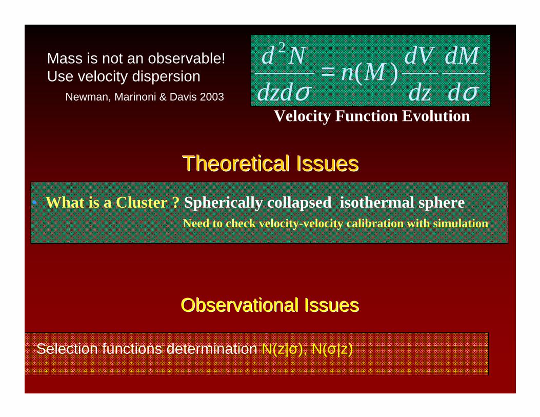
ObservationalObservational IssuesIssues
Selection functions determination N(z|σ), N(σ|z)
• What is a Cluster ? Spherically collapsed isothermal sphereNeed to check velocity-velocity calibration with simulation
Theoretical IssuesTheoretical Issues
Mass is not an observable!Use velocity dispersion
Newman, Marinoni & Davis 2003
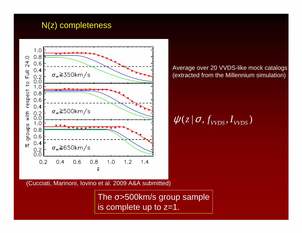
),,|( VVDSVVDS Ifz σψ
N(z) completeness
(Cucciati, Marinoni, Iovino et al. 2009 A&A submitted)
The σ>500km/s group sampleis complete up to z=1.
Average over 20 VVDS-like mock catalogs(extracted from the Millennium simulation)
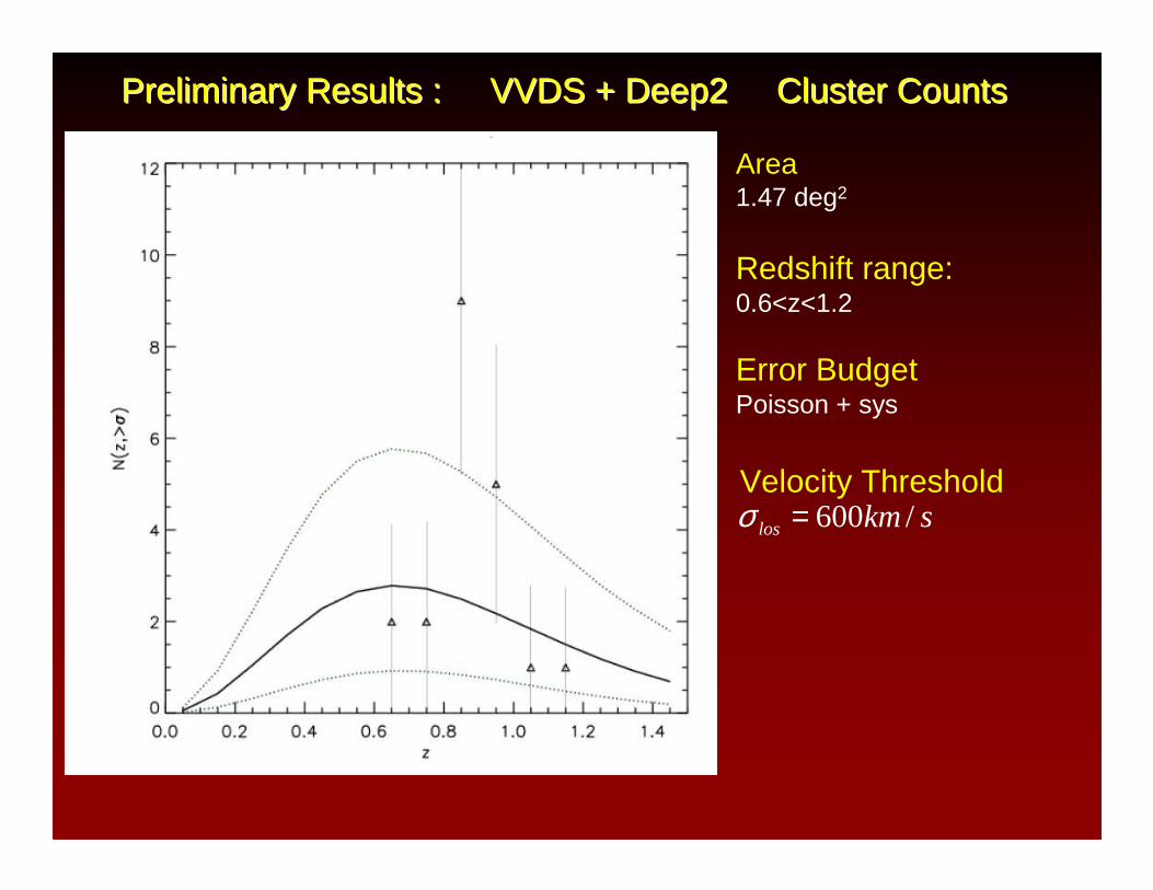
Preliminary Results : VVDS + Deep2 Cluster CountsPreliminary Results : VVDS + Deep2 Cluster Counts
Area1.47 deg2
Redshift range:0.6<z<1.2
Error BudgetPoisson + sys
Velocity Thresholdskmlos /600=σ
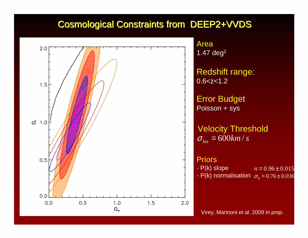
Priors- P(k) slope- P(k) normalisation
015.096.0 ±=n036.076.08 ±=σ
Cosmological Constraints from DEEP2+VVDSCosmological Constraints from DEEP2+VVDS
Area1.47 deg2
Redshift range:0.6<z<1.2
Error BudgetPoisson + sys
Velocity Thresholdskmlos /600=σ
Virey, Marinoni et al. 2009 in prep.
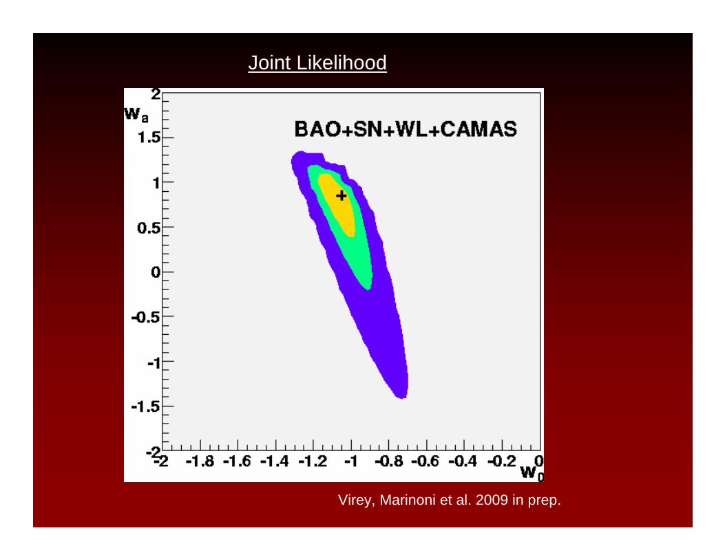
Joint Likelihood
Virey, Marinoni et al. 2009 in prep.
Conclusions
-Evolution of the linear growth factor gives insigths into the nature of DE. Still large errorbars affects VVDS measurements. Need larger deep surveys (e.g. SPACE/Euclide)
Right now : VIPER (P.I. L. Guzzo) 24 sq. deg. N=100,000 galaxies, I<22.5
Conclusions
- semi-linear GIP predictions for skewness evolution are consistent with data in the range 0<z<1.5 only if biasing is non-linear at the level measured by VVDS. If local (z=0) bias is linear GIP ruled out at 5 sigma by current data
-Evolution of the linear growth factor gives insigths into the nature of DE. Still large errorbars affects VVDS measurements. Need larger deep surveys (e.g. SPACE/Euclide)
- Observations underway in the COSMOS/HST field to collect a large sample of velocity selected standard rods (VIMOS @ VLT)and test cosmology with the angular diameter test of cosmology
- Optical Clusters are a unique tool to constrain DE via their velocityfunction evolution. Preliminary results from VVDS+DEEP2 analysis

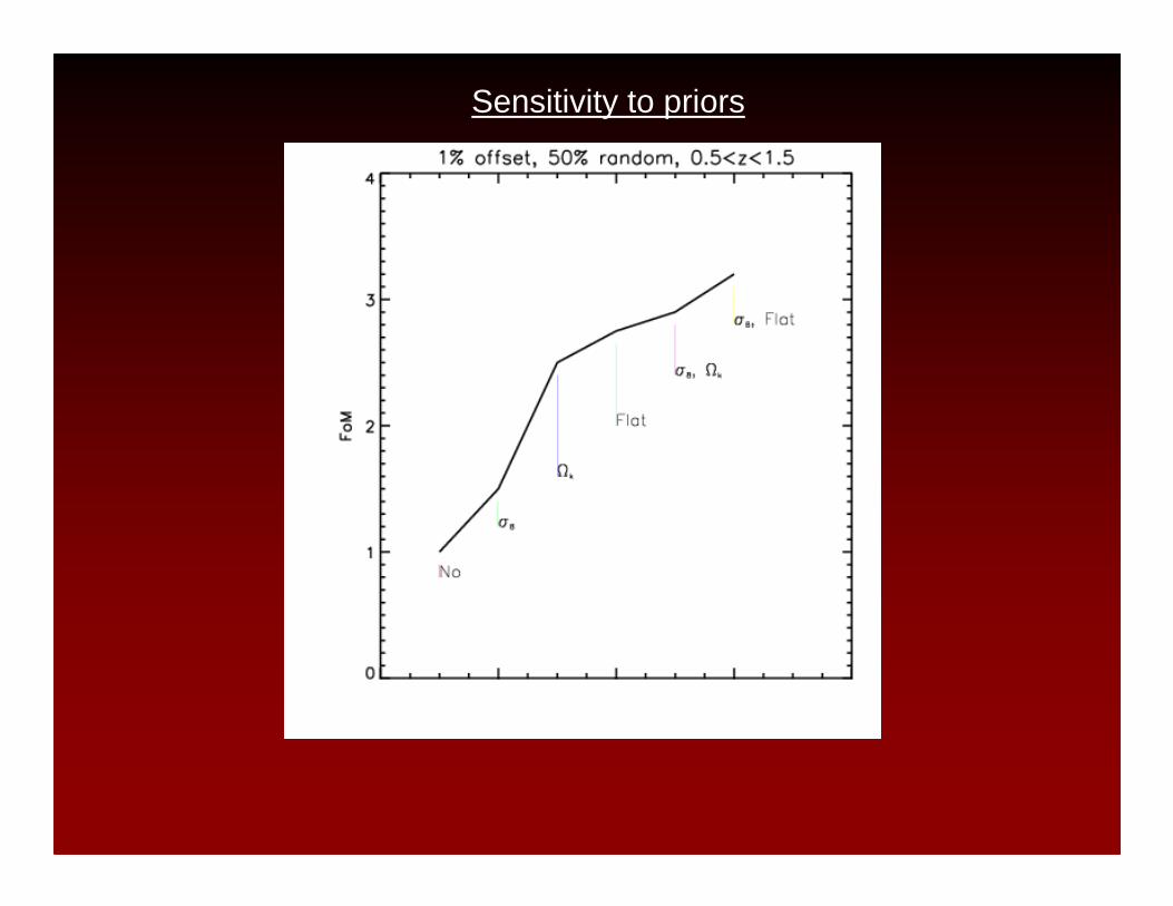
Sensitivity to priors
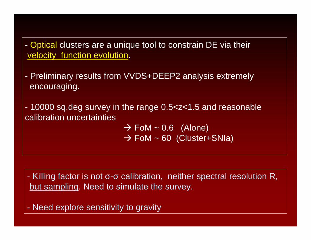
- Optical clusters are a unique tool to constrain DE via their velocity function evolution.
- Preliminary results from VVDS+DEEP2 analysis extremely encouraging.
- 10000 sq.deg survey in the range 0.5<z<1.5 and reasonable calibration uncertainties
FoM ~ 0.6 (Alone) FoM ~ 60 (Cluster+SNIa)
- Killing factor is not σ-σ calibration, neither spectral resolution R,but sampling. Need to simulate the survey.
- Need explore sensitivity to gravity
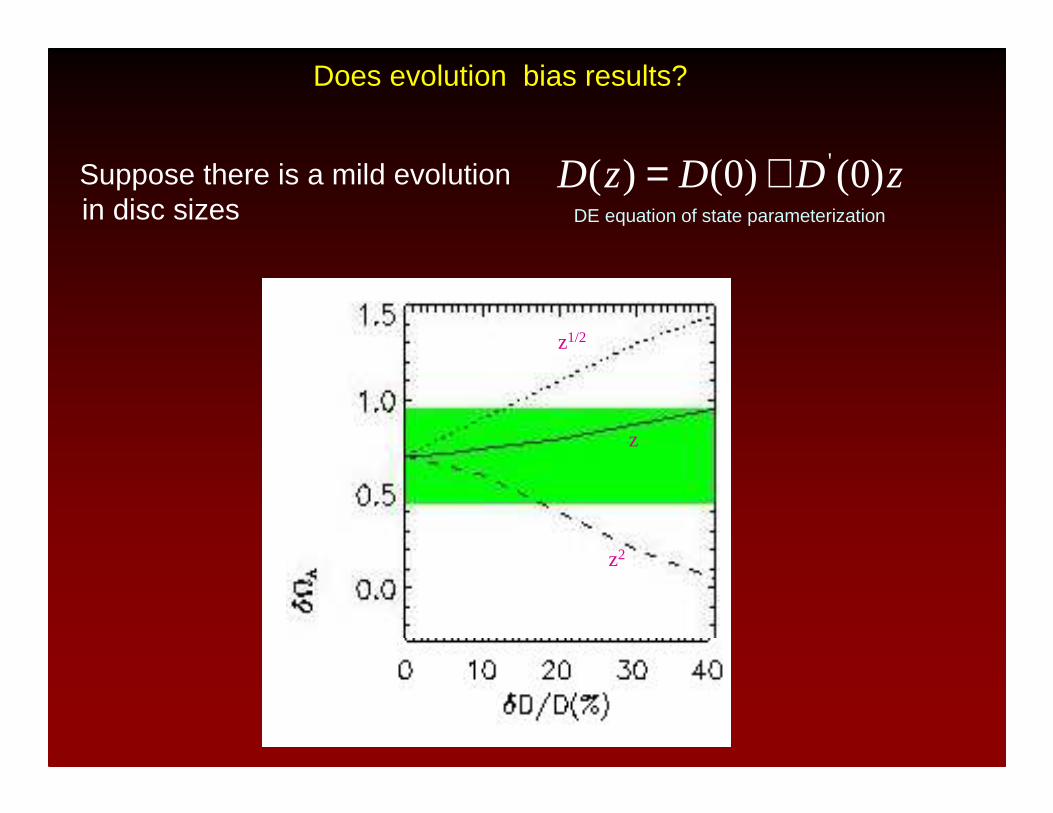
Suppose there is a mild evolutionin disc sizes
Does evolution bias results?
z1/2
z
z2
zDDzD )0()0()( '+=DE equation of state parameterization
PreliminaryPreliminary datadata
1 ,75.0 ,25.0 X -wm ==Ω=Ω
Comparison with thepredicted angularevolution in the standard ΛCDM background
0<v(km/s)<100 100<v(km/s)<200
Standard Rod Selection
Best fitting model
ΛCDM
The PDF of mass: ψ(δ)
Problem: we measure galaxies in redshift space!
Real Space Model Cole & Jones 1991
σz(R,z)
ψ (y) = 1
2πω 2
1y
Exp − [ln y + ω 2 /2]2
2ω 2
y =1+ δ ω 2 = ln[1+ σ r (R,z)2]
σz(z) =σr(0)D(z)[1+ 2
3f (z)+ 1
5f (z)2]
Kaiser 87

Is the lognormal PDF a good approximation?
ΛCDM Hubble Volume simulation (Virgo cons.)