TESTING MODELS OF STRATEGIC UNCERTAINTY:EQUILIBRIUM SELECTION IN REPEATED GAMES

EMANUEL VESPA, TAYLOR WEIDMAN, AND ALISTAIR WILSON

Abstract. In repeated-game applications where both the collusive and non-collusive out-comes can be supported as equilibria, researchers must resolve underlying selection ques-tions if theory will be used to understand counterfactual policies. One guide to selection,based on clear theoretical underpinnings, has shown promise in predicting when collusiveoutcomes will emerge in controlled repeated-game experiments. In this paper we both ex-pand upon and experimentally test this model of selection, and its underlying mechanism:strategic uncertainty. Adding an additional source of strategic uncertainty (the number ofplayers) to the more-standard payoff sources, we stress test the model. Our results affirmthe model as a tool for predicting when tacit collusion is likely/unlikely to be success-ful. Extending the analysis, we corroborate the mechanism of the model. When we removestrategic uncertainty through an explicit coordination device, the model no longer predictsthe selected equilibrium.

1. Introduction

Assumptions about which of the possible equilibria best captures the participants’ eco-nomic behavior take on a central role in applications with repeated interaction. For ex-ample, in models of oligopoly where firms interact repeatedly both collusive and non-collusive equilibria can arise. Researchers must often find evidence in the data to iden-tify which equilibrium best captures the status quo. But equilibrium-selection problemspersist when trying to predict counterfactual behavior, where appeals to the data are notpossible. Consider a market where the researcher can establish that the current behaviorof firms matches the non-cooperative equilibrium, but where their goal is to predict theeffect from industry consolidation on consumer welfare. Embedded within the questionis a concern on whether the selected equilibrium remains the same or will move underthe counterfactual. Were a change isolated solely to the number of firms in the market,a directional comparative-static on selection could be posited: With fewer firms in themarket, ceteris paribus, the equilibrium is likely to be pushed toward greater collusion.

But counterfactual analyses are often more involved than a simple comparative static.In our oligopoly example, while a lower number of firms might push behavior in thecollusive direction, consolidation tends to be accompanied by other concurrent changes.For example, bigger firms can generate efficiency gains, increasing the marginal returnsto price competition and product innovation. These accompanying shifts to the profit

Date: January, 2021.We would like to thank: David Cooper, Guillaume Fréchette, Daniella Puzzello and Lise Vesterlund.

This research was funded with support from the National Science Foundation (SES:1629193).1

arX

iv:2

101.

0590

0v1

[ec

on.G

N]

14

Jan

2021

functions could plausibly pull more towards the non-collusive equilibria.1 As such, con-solidation has the potential for conflicting effects on the likelihood of collusion. Morebroadly, whenever counterfactual policies involve richer changes to more than one vari-able, predicting the resulting effect on the selected equilibrium can become substantiallymore challenging.

In this paper we evaluate a model of equilibrium selection constructed over the theoreti-cal primitives; a model capable of integrating counterfactual shifts to many primitives atthe same time. In doing this, we build on experimental studies of the infinitely repeatedprisoner’s dilemma (RPD), where strategic uncertainty has been offered as an explanatorymodel for rationalizing several findings across this literature. Specifically, Dal Bó andFréchette (2011) outline the organizational power of a selection notion from Harsanyi andSelten (1988) when applied to data from their experimental treatments.2 The central ideahere is to formally model the strategic uncertainty surrounding the collusive, history-dependent, equilibrium. In so doing, the analyst can reduce the equilibrium-selectionproblem to an understanding of the risk/reward trade-off over collusion attempts. Thedeveloped strategic-uncertainty measure is therefore a pure function of the primitivesof the game. Thus, the model can help understand the trade-offs between two or morecompeting shifts of the primitives—for example, a change to the payoffs that increasesthe rewards to successful collusion combined with a reduction to the discount rate thatmakes such an attempt riskier. The model mediates the effects of any multivariate changeinto a single dimension, the effect on strategic uncertainty, which can then be used topredict the eventual likelihood of collusion. However, while the literature has shown theexplanatory power of the strategic-uncertainty measure, previous studies have not beendesigned to test it, to examine the mechanism, and its potential limitations.

To stress test this equilibrium-selection model we expand the set of primitives underconsideration. In so doing we introduce a new source of strategic uncertainty to therepeated environment, one that plays an important role in applications, as motivatedby our industry consolidation example above. Similar to the original two-player RPDexperiments, our treatments will manipulate payoff primitives (primarily a stage-gamepayoff-parameter x) that affects the riskiness of collusion. But we also manipulate thenumber of players within the environment (N ), where collusion in the model becomesriskier in larger groups. Hence, we can study joint changes in both x and N—changesthat push the equilibrium selection in two different directions, where the model’s abilityto predict the joint effect is the object of interest. As such, we will test the main hypothe-sis that equilibrium-selection across two distinct sources can be understood through thestrategic-uncertainty model. We therefore construct treatment manipulations that mod-ify x and N relative to a baseline in a way that the strategic-uncertainty measure is heldexactly constant. Finding constant cooperation across the double-barreled change would

1The industry-consolidation literature provides ample evidence that mergers are regularly accompanied byother changes in addition to a lower number of market participants. For instance, accompanying effectsinclude lower costs (Farrell and Shapiro, 1990), higher capacities (Perry and Porter, 1985), new productofferings (Deneckere and Davidson, 1985), and asymmetry among firms (Compte, Jenny, and Rey, 2002).2A subsequent meta-study across the literature (Dal Bó and Fréchette, 2018) confirmed the pattern.

2

be consistent with the modifications to x and N being perfect substitutes, per their mod-eled effect on strategic uncertainty.3 Complementing the construction and test of the corestrategic-uncertainty model, our design also embeds an alternative hypothesis (which wecharacterize the behavioral underpinnings of) in which the group-size variable N doesnot affect strategic uncertainty, with a clearly distinct set of predictions from our mainmodel.

Our main results allow us to clearly separate and validate the equilibrium-selection modelbased on strategic uncertainty. Across the six possible treatment comparative-statics inour design, four are predicted to have clear directional effects on selection (with the othertwo being perfect substitutes). In every single one of these four comparisons, data fromour experiments move in the predicted direction, with effects sizes that are both statisti-cally and economically significant. This is true for both initial and ongoing behavior forthe repeated games we examine. The more-challenging comparisons involve treatmentswith compound shifts that move selection in opposed directions. Two of our treatmentcomparisons are constructed so that changes across the payoff and group-size are per-fectly substituting as captured by the strategic-uncertainty model. Relative to successfulcoordination on the collusive outcome, the metric that likely matters most for applica-tions, our results show strong support for the selection model, and our designed shiftsto the payoffs and number of players are direct substitutes. Meanwhile, we documentdiscrepancies between the measure’s predictions and behavior in the first period of inter-action. As such, our results indicate that the extended selection model is more accuratein predicting ongoing collusion than in predicting initial intentions—where changes inN provide the key variation to identify this. Overall, our results validate the theoreticalmodel, providing a tool to understand which effects might dominate in counterfactualswhere policy shifts over multiple primitives. In particular, the results lend credence tothe idea that a reduction of the environment to a single dimension capturing strategicuncertainty can be predictive of equilibrium selection.

Uncertainty regarding the other players’ actions is put front-and-center in our main treat-ments as the driver of equilibrium selection. Hence, if strategic uncertainty is the causalmechanism driving selection, then removing or reducing the doubts about others’ playshould make the selection model’s predictions moot. We pursue this idea in an addi-tional set of treatments where we allow for pre-play communication in a setting wherewe would otherwise expect little collusion. Participants are given the opportunity toexchange free-form messages prior to the repeated game, a feature that can be used toreduce uncertainty over others’ intentions (see Kartal and Müller, 2018). For the sameexperimental parameterization where we observe ongoing cooperation rates below onepercent without communication, the effect from adding it is to shift behavior to the otherextreme: with initial (ongoing) cooperation rates of 95 (80) percent.4 Given these results,

3Our treatments also include manipulations where the strategic-uncertainty effects of one of the two vari-able changes theoretically dominates the competing effect, with a predicted effect on selection. Moreover,the design also embeds comparative-static comparisons where a single variable is manipulated.4As a check that the provided communication channel is not driving results separate from the equilibriumcoordination effects, we implement a second treatment with communication but where the collusive out-come is not a robust equilibrium outcome. Here we find that communication does not lead to successful

3

we conclude that strategic uncertainty, the mechanism underlying the model, is the causalchannel. In addition to mechanism validation, these results clearly outline the limitationof the model to understanding tacit collusion, in the sense that it fails to provide usefulguidance when collusion is more explicit.

In terms of the paper’s organization, we next outline the related literature. In section 2we outline our generalization of the selection model from the two-player repeated PDgame, outline the predictions from that literature, and provide design details. In section4 we analyze the results from our core treatments and demonstrate the model’s predictiveproperties generalize to N . Section 5 then examines some extensions: one showing thatour results hold for both between- and within-subject identification; and the other pin-ning down the strategic uncertainty mechanism via the opportunity for explicit collusion.Finally, in section 6 we conclude.

1.1. Literature. Our paper builds on the recent consolidation of the experimental RPDliterature presented in Dal Bó and Fréchette (2018). While one of our baseline treatmentsreplicates a standard finding in the literature,5 our core contribution is to generalize theequilibrium selection model outlined in the meta-study, adding an additional source ofstrategic uncertainty: the number of players, N .6 Where the literature has developed thismodel to be explanatory, our approach is both to expand the selection model to a newsetting, but also to take the model as the core experimental object to be tested.

Our generalization of the strategic uncertainty model in the RPD literature is carried outin two alternative ways. The first extension (and most-standard, given its use of indepen-dent beliefs) formalizes a distinct source of strategic uncertainty from the payoff-basedsource in the meta-study. An alternative extension (based on fully correlated beliefs)reflects a null effect, that the newly introduced source has no effect. As such, our gen-eralization offers a potentially profitable design approach for future research examiningother channels for strategic uncertainty effects—asymmetries in the action space or pay-offs, the effects of sequentiality, etc.7

Our environment also allows us to better distinguish between the empirical measureslinked to the selection model. That is, using literature-level data assembled by Dal Bó andFréchette (2018), we show that the two-player RPD strategic uncertainty model predictsboth initial and ongoing cooperation well. However, neither is identified particularly wellfrom the other. With more than two players though, this is no longer the case, where we

collusion. In other words, communication only has an effect when there are clear theoretical incentives forcollusion.5As pointed out in Berry, Coffman, Hanley, Gihleb, and Wilson (2017) many experimental replicationsbecome harder to find where the papers do not explicitly point out the replication components.6The extension of the notion of equilibrium selection described in Harsanyi and Selten (1988) to the RPDwas first proposed by Blonski and Spagnolo (2015) and first shown to organize data by Dal Bó and Fréchette(2011). See also Fudenberg, Rand, and Dreber (2010) for an examination of the effects with imperfectmonitoring, and Kartal and Müller (2018) for a test of a selection theory based on individual heterogeneityin preferences over dynamic strategies.7See Ghidoni and Suetens (forthcoming) and Kartal and Müller (2018) for experimental examinations theeffect sequentiality has in RPD settings through a reduction in strategic uncertainty.

4

use this to demonstrate that the developed strategic uncertainty model is better suitedfor predicting successful collusion rather than initial intentions.8

This paper is part of a broader literature seeking to understand and document regulari-ties in equilibrium selection. In particular, regularities that are amenable to theoreticalmodeling. To this end, the strategic-uncertainty measure that we examine is particularlypromising, as the equilibrium objects required for calculation are computationally sim-ple: the stationary non-collusive equilibrium and the history-dependent collusive equi-librium. In environments beyond the RPD where the equilibrium outcomes are heldconstant, the model can be similarly extended per our illustration with a move to N play-ers. However, in more complex environments where the equilibrium set changes moresubstantively, the constraint to two focal equilibria in the strategic uncertainty modelmay lose validity, and/or raise questions as to which two strategies are focal. Exam-ples of more-complex settings includes dynamic games, where the stage environmentcan change across the supergame and the space of strategies becomes substantially larger.Vespa and Wilson (2020) focus on a horse-race examination of which two equilibria arefocal (from a wider set of possible alternatives) for rationalizing behavior in dynamicgames. The paper identifies a similar strategic uncertainty measure constructed aroundthe most-efficient Markov perfect equilibrium and the best symmetric collusive equilib-rium. A strategic-uncertainty model based on these strategies predicts behavior, wherethese strategies dovetail with the repeated-game strategies in the simpler environmentstudied here.9

An experimental literature on behavior in oligopolies documents that collusion clearlyresponds to the number of players. Both Cournot (Huck, Normann, and Oechssler, 2004;Horstmann, Krämer, and Schnurr, 2018) and Bertrand settings (Dufwenberg and Gneezy,2000) indicate that as the number of players increases collusion becomes less likely, oftenas soon as N exceeds two.10 We contribute to this literature on two margins. First, papershere focus on out-of-equilibrium behavior in settings with a finite-time horizon, and asubsequently unique theoretical prediction. In contrast, we examine how changes to Naffect outcomes in an infinite-horizon environment with both collusive and non-collusiveequilibria. Second, and crucially, our focus is not just on the qualitative directional ef-fects from N , but on validating a model of how it affects strategic uncertainty. The modelallows for an understanding of the extent of substitutability between primitives underconsideration; and where validated can predict the directional effects of more-nuanced,multi-dimensional counterfactuals. Clearly, any equilibrium-selection notion suggestedfor such a task requires a great-deal of scrutiny. However, our findings do suggest sub-stantial optimism that this path may be fruitful.

8Ongoing cooperation is a measure that is likely to be more relevant for empirical applications wherecollusion may be a worry. For instance, from Harrington, Gonzalez, and Kujal (2016), page 256: “(...)collusion is more than high prices, it is a mutual understanding among firms to coordinate their behavior.(...) Firms may periodically raise price in order to attempt to coordinate a move to a collusive equilibrium,but never succeed in doing so; high average prices are then the product of failed attempts to collude.9Work on equilibrium selection in dynamic games builds on recent contributions in this area. For example:Battaglini, Nunnari, and Palfrey (2012, 2016); Agranov, Frechette, Palfrey, and Vespa (2016); Kloosterman(2019); Vespa and Wilson (2019); Rosokha and Wei (2020); Salz and Vespa (2020); Vespa (2020).10See also references in Potters and Suetens (2013) for similar findings.

5

Our work is also related to an experimental literature on mergers that manipulates thenumber of players. As surveyed by Goette and Schmutzler (2009), some experimentsdeal with a “pseudo-mergers,” where a subset of the original firms remain in the market(Huck, Konrad, Müller, and Normann, 2007, for example). Others experiments imple-ment “real mergers,” where mergers introduce other changes in the market beyond N(Davis, 2002). A contribution of our approach is that the strategic-uncertainty measurecan predict counterfactual behavior in both settings. Another discussion in this literatureis whether merger effects are evaluated within the same group of participants (within-subject designs) or across different groups (between-subject design). In this paper, whileour main treatments make use of between-subject identification, we also conduct within-subject sessions at the same parameterization, demonstrating that though there can bemeaningful short-run differences, with enough experience the results do not depend onthe approach.11

The effects of communication devices as a bolster for collusion are well-established inthe experimental literature. As surveyed in Cason (2008) and Harrington, Gonzalez, andKujal (2013), more-structured, limited forms of communication usually result in small,temporary collusive gains, where free-form communication generates large, long-lastingeffects.12 For these reasons, in one of our extensions we examine unrestricted chat mes-sages as a strong coordination device. The collusive results here clearly indicate that thedomain for our strategic-uncertainty measure based on tacit-collusion does not includeenvironments where explicit collusion is likely. However, we do show that there are clearlimits on the effects of explicit collusion, and that these limits are directly predicted bytheory. Using a change to the payoff primitives (here the discount rate) we make collu-sion a knife-edge, non-robust equilibrium, and show that the effects of communicationare entirely dissipated.

While much of the literature on repeated games studies the standard two-player PDgame, there is a large literature studying a canonicalN -player social dilemma: the volun-tary contribution public-goods game (see Vesterlund, 2016, for a survey). Though muchof this literature focuses on finite implementations, one notable exception is Lugovskyy,Puzzello, Sorensen, Walker, and Williams (2017). Similar to our paper, the authors useexperimental variation over both N and the payoff primitives (in their case the return togroup contribution). However, this is done with a different end goal. They design off-setting variation in the payoffs and N to identify the isolated effect of the stage-game’sMPCR. We instead do so to isolate strategic uncertainty, to test a predictive theory ofselection.

11Differences in behavior can be stickier if changes are small or introduced gradually. Weber (2006) showsthat increasing the number of players gradually in a coordination game leads to different results relativeto a situation when play starts with a large group. In repeated games gradual introduction of changesto the payoff primitives have also been found to have effects in repeated games, see Kartal, Müller, andTremewan (2017). These results suggest that the selection-notions we are examining are relevant for ‘large’counterfactual changes, and where future research can help clarify how to integrate ‘large’ into a predictivemodel of selection.12For further details on the effect of communication in repeated games with an unknown time horizon, seeFonseca and Normann (2012), Cooper and Kühn (2014), Harrington et al. (2016), Wilson and Vespa (2020)and Fréchette, Lizzeri, and Vespa (2020).

6

Beyond social dilemmas, our paper is also connected to the literature on coordinationgames (see Devetag and Ortmann, 2007, for a survey). The strategic-uncertainty measureexamined in our paper works because the infinitely repeated prisoner’s dilemma gamehas a stag-hunt normal-form representation (Blonski and Spagnolo, 2015), adapting therisk-dominance notion for one-shot coordination games in Harsanyi and Selten (1988).13

Risk dominance (and the cardinal implementation through the measure of strategic un-certainty) has been shown to have substantial predictive content in simple coordinationgames with trade-offs over payoff-dominance and risk-dominance (see Battalio, Samuel-son, and Van Huyck, 2001; Brandts and Cooper, 2006, and references therein). Strategicuncertainty has therefore demonstrated its usefulness as a theoretical selection deviceboth in directly presented one-shot games, and in repeated games. Our contribution tothis literature is to design an experiment to explicitly test it and show that the predictiveeffects extend further still, to multi-player infinite-horizon settings.

2. Generalizing the Basin of Attraction

Developing empirical criteria for equilibrium selection in games where collusion is pos-sible requires two measures: one theoretical, one empirical. On the theory side we needa prediction, a model that maps the primitives of the game into a scalar where up-ward/downward movements are clearly interpretable as increasing/decreasing the like-lihood of collusion. On the empirical side we need a precise target against which thetheoretical notion can be contrasted and validated. This empirical measure should exam-ine a behavior that differs starkly under the collusive and non-collusive equilibria.

We begin this section by summarizing the progress made towards validating a theoreticalprediction in the two-player infinitely repeated prisoner’s dilemma (RPD) literature. Thetheoretical notion here is the size of the basin of attraction for the strategy always defect.The focal outcome measure is the cooperation rate of individual players in the initialrounds. In what follows we discuss the issues as we extend the exercise to a new sourceof strategic uncertainty, the number of players N—both for the theoretical and empiricalmeasures.

2.1. Two-players. Consider an RPD with discount rate δ ∈ (0,1). In each period t =1,2, . . . players i ∈ {1,2} simultaneously select actions ai ∈ A :={(C)ooperate, (D)efect}.The period-payoff for player i is a function of both players’ choices, πi(ai , aj), where allsymmetric PD games can be expressed in a compact form by normalizing all payoffsrelative to the joint-defection payoff π0 = π(D,D), and rescaling with the relative gainfrom joint cooperation: ∆π := πi(C,C) − π0.14 Defining scale and normalization in thisway, the PD stage-game can be expressed with two parameters g and s for the different-action payoffs πi(D,C) = π0+(1+g)∆π and πi(C,D) = π0−s ·∆π. The parameters g > 0 ands > 0 thereby capture the relative temptation- and sucker-payoff parameters, respectively.

13The difference in our setting is that neither total payoffs nor strategic choices are directly provided toparticipants, as these are extensive-form objects. Instead they are provided with the stage-game pay-offs/actions, where strategies (such as the grim trigger or tit-for-tat) and gross payoffs must be endogenouslyformulated.14More exactly, game payoffs π can be transformed via π̃ = (πi −π0)/∆π to measure all payoffs relative tojoint defection in units of the optimization premium.

7

The RPD payoffs can be used as primitive inputs into a risk/reward model of collusionbased upon strategic uncertainty. Strategic uncertainty here is distilled into a decisionbetween two focal extensive-form RPD strategies:

(i) Always defect, αAll-D, which plays the stage-game Nash in all rounds (the uniqueMPE of the game).15

(ii) The Grim Trigger, αGrim, a strategy that begins by cooperating but switches toalways-defect after observing any defections in past play (the best-case collusiveSPE).16

As functions of the observable history ht, these two strategies are given by:

αGrim(ht) ={C if t = 1 or ht = ((C,C), (C,C), . . . , (C,C)),D otherwise;

αAll-D(ht) =D.

Strategic uncertainty in the two player RPD is measured through the size of the basin ofattraction for always defect. The model considers the expected payoff to player i whenuncertainty on the other player j is represented by a believed strategy mixture p ·αGrim ⊕(1−p)·αAll-D. The basin for always defect is defined as the set of beliefs p for which player iyields a higher expected payment from αAll-D than αGrim. The always-defect belief basin istherefore the interval [0,p?(g,s,δ)], where the critical-point/interval-width is given by:17

(1) p?(g,s,δ) ≡ (1− δ) · sδ − (1− δ) · (g − s)

.

The basin-size p?(g,s,δ) has a clear interpretation for strategic uncertainty: for any beliefp > p?(g,s,δ) on the other player using the collusive strategy αGrim, the player does strictlybetter choosing αGrim; for any belief p < p?(g,s,δ), they do strictly better by selecting thenon-collusive strategy αAll-D. As such, the smaller p? is, the lower the strategic uncertaintysurrounding collusion. Moreover, the cardinal basin-size measure directly implies theordinal risk-dominance relationship between the two strategies. If p?(g,s,δ) < 1/2 thenthe collusive strategy αGrim risk-dominates αAll-D, and vice versa. Henceforth, by ‘basin ofp? ’ we mean the maximal belief on the other cooperating for which the strategy αAll-D isoptimal.

Equation (1) represents an easy-to-derive theoretical relationship between the payoff prim-itives of the game (here g, s and δ) and a critical strategic belief on the other player’s likeli-hood of collusion. The hypothesized relationship is monotone, where the higher is p? , the

15A Markov strategy is history independent, removing any conditioning on past play. A Markov-perfectequilibrium (MPE) is a subgame-perfect equilibrium (SPE) in which agents use Markov strategies. In anRPD, if choices are forced to be history independent then there is a unique equilibrium: playing the stage-game Nash equilibrium in all periods.16The strategy here is ‘best case’ in three senses: (i) it can support the best-case outcome; (ii) it uses theharshest possible punishment, and so can support collusion at smaller values of δ than any other strategy;and (iii) any realized miscoordination is minimal, being resolved in a single round.17In the case that the strategy (αGrim,αGrim) is not an SPE of the repeated game, the basin size for alwaysdefects is defined as p?(xT ,xS ,δ) = 1.

8

(a) Initial cooperation (b) Ongoing cooperation

Figure 1. Meta-study relationship: Strategic Uncertainty and RPD Cooper-ation

Note: Figures show estimated effects and 95-percent confidence intervals for initial/ongoing cooperation inRPD meta-study (Dal Bó and Fréchette, 2018). Red dashed line in Panel (B) indicates implied theoreticalrelationship for ongoing cooperation based on the estimated relationship illustrated in Panel (A). Eachpoint indicates a separate treatment, with the number of participants indicated.

lower is the likelihood of cooperation, thereby allowing for unambiguous directional pre-dictions for any counterfactual change in the primitives. The posited mechanism withinthis model is also clear-cut: strategic uncertainty introduces a risk/reward trade-off forcollusion attempts, which can be solved using standard economic analysis. This has twobenefits: First, we can test the underlying strategic-uncertainty mechanism through otherchannels outside of the model, where we will do exactly that in an extension examiningcoordination devices. Second, the necessary assumptions for extending this model toanalyze alternative strategic-uncertainty sources are straightforward.

We now turn to the empirical criteria used to validate this theoretical measure. As asummary of the RPD literature we focus on the recent meta-study on the two player RPD(Dal Bó and Fréchette, 2018). Two of the main results here are to show that the scalarbasin-size measure of strategic uncertainty is highly predictive of behavior, though witha non-linear relationship. We illustrate this relationship in Figure 1 for two empiricaloutcome measures.

In both panels in Figure 1 the theoretical measure of strategic uncertainty (the basin-size p?) is presented on the horizontal axis. The empirical outcome measures are pre-sented on the vertical axes. In Panel (A) we present the results for initial cooperation inthe supergame, a measure tracking collusive intentions at the individual level as there isno interaction with matched partners at this point. In contrast, in Panel (B) we present

9

results for ongoing cooperation, choices in rounds two and beyond, a measure of the ex-tent to which collusion attempts are successful. While there is no mechanical relation-ship between initial and ongoing cooperation, the theoretical model used in the basinconstruction posits an indirect linkage between the two. If collusion functions throughconditional-cooperation with grim-trigger punishments, then the expected ongoing co-operation rate is the probability that the players jointly cooperate in the first round: theinitial cooperation rate all squared. Thus, the posited relationship between initial andongoing cooperation in the two-player RPD is not separately identifiable through any ofthe underlying payoff primitives.

Using the meta-study data from 996 participants across 18 experimental treatments, weestimate the relationship between late-session cooperation (supergames 16–20, the datawe focus on in our experiments) and the strategic-uncertainty basin-size measure. Per themeta-study, the fitted relationship is estimated using a piecewise–linear probit model.18

The solid line in each figure indicates the predicted cooperation rate at each p? from theprobit estimates, where the shaded region indicates the 95 percent confidence intervalfor the prediction (clustering by treatment). For both initial and ongoing cooperation thesame pattern is found: a consistently low cooperation level when always-defect is risk

dominant (p? >12

); and a significantly decreasing relationship with p? when collusion is

risk dominant (p? <12

). As such, Figure 1(A) illustrates Results 3 and 4 from the meta-

study.

Figure 1(B) indicates a similar qualitative relationship between strategic uncertainty andongoing cooperation. Going beyond just the form though, layered on top of the estimatedongoing-cooperation relationship we also indicate the implied theoretical relationshipwith the initial-cooperation results. Using the square of the estimated initial cooperationrate given in Panel (A) we therefore calculate the predicted joint cooperation rate in roundone. Under grim-trigger coordination, the initial joint-cooperation rate is exactly the on-going cooperation rate, and so we illustrate this implied relationship in Panel (B) as thered dashed line. There are certainly some differences between the estimated relationshipusing actual ongoing cooperation decisions (black solid line) and the implied rate frominitial cooperation (red dashed line). However, as the figure illustrates, these differencesare mostly in levels for the region where always-defect is risk dominant.19 Slopes and

levels for p? in the [0,12

] region where the strategic uncertainty input has a clearer empir-

ical response are not significantly different. The implication from this is that with onlytwo players we cannot separately identify the extent to which the strategic-uncertainty

18Individual-level cooperation decisions are the left-hand side variable, where the basin-size enters theright-hand side in a piecewise-linear fashion around the risk-dominance dividing point. The econometricspecification is motivated by Dal Bó and Fréchette (2018, Table 4); however to enforce level-continuityin the estimated relationship we remove a degree of freedom from their specification that allowed for adiscontinuity at p? = 1/2.19In particular, we find significantly more ongoing cooperation when the basin measure is above 1/2 thanwe might expect from the initial rates and the use of a grim-trigger. This is consistent with another findingin the literature, the frequent use of more-forgiving/lenient strategies than grim. Tit-for-tat, for instance,can generate substantial ongoing cooperation when matched with its variant that starts out defecting.

10

measure is predicting initial intentions and/or successful coordination. However, as wewill show, adding more players provides a channel to identify between the initial andongoing measures.20

2.2. Extending to N > 2. We now extend the strategic-uncertainty model above to anN -player environment. The core extension is intuitive: instead of considering one otherplayer choosing a mixture p ·αGrim⊕(1−p)·αAll-D, we considerN −1 other players choosingthis same strategic mixture.

To outline the extension, and set-up our design, we consider a family of symmetric socialdilemmas that nest the standard RPD when N = 2. However, to hold constant a 2 × 2stage-game representation for all N , our family of dilemmas make use of an aggregate(and deterministic) signal of the other agents’ actions. Each player i = 1, . . . ,N continuesto make a binary action choice ai ∈ A ≡ {C,D}, but their payoffs do not vary with (andthey do not receive feedback on) the separate actions of the other N − 1 players. Instead,payoffs are determined by the own-action ai and a deterministic binary signal σ (a−i) ∈{S(uccess),F(ailure)} of the others’ actions, a−i . In particular, the generic player i’s stage-game payoff and signal function are given, respectively, by:

πi(ai ,σ

)=

π0 +∆π if ai = C,σ = S,π0 +∆π · (1 + x) if ai =D,σ = S,π0 −∆π · x if ai = C,σ = F,π0 if ai =D,σ = F;

σ (a−i) ={S if aj = C for all j , i,F otherwise.

These choices lead to a symmetric game, where payoffs can be summarized with a 2 × 2table over: (i) the own action C or D; and (ii) the signal outcome, an S signal if the otherN − 1 players jointly cooperate, or an F signal if at least one matched player defects. Theexact payoffs (with the same implicit scale ∆π and normalization π0 as before) implementa PD-like environment where payoff-based strategic uncertainty is collapsed to a singleparameter x.21

The success/failure signal here is a deterministic function of the N − 1 other player’s ac-tions that dovetails with the standard RPD game when N = 2. The choice for the signalfunction σ (·) here maximizes the coordinative pressure, duplicating a Bertrand-like ten-sion: collusion is successful only when the other N − 1 players all cooperate.22

20For any setting where collusion requires N agents to initially cooperate to produce ongoing cooperationthen the relationship is simply initial cooperation rate to the N -th power. Separate identification betweenthe two measures then comes about through comparison across treatments with different values of N .21In the meta-study notation this is implemented with s = g = x. This single-parameter formulation isequivalent to the Fudenberg et al. (2010) benefit/cost formulation, where their benefit/cost ratio b/c pa-rameter is given by (1+x)/x here.22While potentially interesting, one disadvantage of a Cournot-like parameterization where the positiveexternality from others’ cooperation is strictly increasing in the number of cooperators is that the cardinal-ity of the signal/history spaces will then scale with N . However, note that the precise basin-size formula

11

Ignoring the game’s scale and normalization (held constant in our experiments with ∆π =$9 and π0 = $11) the repeated games we examine are summarized by three primitives: (i)The relative cost of cooperating, x. (ii) The number of players, N . (iii) The continuationprobability, δ. Our experiments will fix δ = 3/4 in all but one diagnostic treatment in theextensions section. This leaves us with two key experimental parameters: the relativecost x (actual cost X = x∆π) and the number of participants N .

In building a model of strategic uncertainty for arbitrary N , we will use a symmetricbelief over the others’ choices. That is, we assume each player chooses a mixture p ·αGrim⊕(1−p) ·αAll-D over the two strategies.23 Our family of social dilemmas require cooperationfrom all N players for everyone to get a success signal. Because of this, the strategicuncertainty reduces to the probability that the other N − 1 players jointly coordinate onthe collusive strategy,

Q (N ) = Pr {N − 1 others all choose αGrim} .

In every other case a failure will be received by at leastN −1 players, and the punishmentpath will be triggered.

In an identical manner to the two-player case, the critical belief Q?(N ) is given by thepoint of indifference between the amount given up with certainty from a single round of

cooperation, x ·∆π, and the continuation gain from collusion,δ

1− δ·∆π, obtained with

probability Q(N ). Indifference is therefore given by:

Q? (N ) =(1− δ)δ

x,

where the RHS is identical to the two-player construction in (1) for x = g = s.

To complete the extension we therefore need to relate the joint-cooperation of the otherN −1 players to the probability p that each other player individually attempts to collude.However, even though we have specified the marginal belief distribution and assumedsymmetry, we must still resolve the relationship between the joint and marginal distribu-tions: the extent to which beliefs are correlated. In particular our design and extensionwill focus on two extreme models as we extend the model toN -players. The ‘standard’ ex-tension, where beliefs are fully independent; and an alternative/null-effect model where

is identical under the Cournot formulation if own cooperation has an additive cost x ·∆π and the punish-ment path is triggered on any level of defection. An alternative choice for a signal σ (·) that does not scalewith N would be that successes are achieved whenever some minimal number of players cooperate (≥ 2say). Notice though, that such a choice introduces a second coordination problem over who cooperatesand who defects. Efficiency requires the minimal number of cooperators, with the rest free riding. Chang-ing the signal function in this way would therefore introduce a distributional asymmetry (see Wilson andVespa, 2020, for an illustration that these additional dimensions lead to non-trivial problems). Given ourfocus on understanding the effects from adding a new source of strategic uncertainty, we therefore chosean environment that did not introduce additional trade-offs/confounds.23For the N -player dilemma we define the grim-trigger strategy with imperfect-signals as:

αGrim(ht) =

C if t = 1 or ht = ((C,S), (C,S), . . . , (C,S))D otherwise.

12

beliefs are perfectly correlated.24 Assuming perfect correlation for the other N −1 agents,joint and individual probabilities are identical, Q (N ) = p, and so the extended criticalbelief (and correlated model outcome) is given by:

(2) p?Corr.(x) =1− δδ· x.

In constrast, when the beliefs are independent we have Q (N ) = pN−1, and the criticalbelief (and independent model extension) is:

(3) p?Ind.(x,N ) =(1− δδ· x

) 1N − 1 ≡

(p?Corr.(x)

) 1N − 1 .

Obviously, when N = 2 the basin measures in (2) and (3) are identical, dovetailing withthe standard construction. However, for N > 2 the two measures of strategic uncertaintyare distinct, where the standard model extension under independence has strategic un-certainty vary both through the payoff parameter x and the group-size N .

3. Experimental Design

The basin of attraction for always defect under independent beliefs serves as our measureof strategic uncertainty. Ceteris paribus, the greater the uncertainty on successful strate-gic coordination, the more likely the subject is to take refuge in the safer strategy—in thecase of an RPD game, the stage-game Nash outcome of defecting.

As outlined above, as we extend the environments toN > 2, this opens up a question as tohow strategic uncertainty is affected by N . If others’ behavior is thought to be highly cor-related, adding players but holding constant the payoffs will do little to affect the selectedbehavior in our games. If this is so, the null-effect p?Corr. measure of strategic-uncertaintywill predict behavior. In contrast, in a more-standard extension where beliefs on the otherplayers are independent, then p?Ind. will model the strategic uncertainty. Under this exten-sion, we will be able to use shifts in p?Ind. to understand changes in the selected behavior.While one implication of this is that the addition of more players will ceteris paribus re-duce collusion, a deeper implication of the model is to help us understand substitutioneffects across the two sources of strategic uncertainty, x and N .

Our experimental design attempts to untangle the effects of strategic uncertainty. Theaim of the design is to embed comparative-static tests on the effect of N (and so rule outthe p?Corr. null-effect model), but also to examine the possible substitution effects by con-structing perfect-substitutes treatments with the p?Ind. model. We achieve this through aseries of experimental implementations of the N -player 2-action–2-signal repeated gameoutlined above. In particular, the first part of our design will use this family of games todistinguish and separate between the two extremes of independence and perfect correla-tion, leveraging the theoretical relationships derived above.

While we cannot directly manipulate strategic uncertainty—as the basin-size measuresare indirect, theoretical relationships derived from the primitives—equations (2) and (3)

24See Cason, Sharma, and Vadovič (2020) for a clear example of correlated beliefs arising where indepen-dence would be the standard prediction.

13

Table 1. Experimental Design

Panel A. Stage-gamepayoffs

X = $9 X = $1

σ (a−i) = S σ (a−i) = F σ (a−i) = S σ (a−i) = F

Coop., πi(C,σ ) $20 $2 $20 $10Defect, πi(D,σ ) $29 $11 $21 $11

Panel B. All-D BasinSize

X = $9 (x = 1) X = $1 (x = 1/9)

N = 2 N = 4 N = 4 N = 10

Cor. basin, p?Cor.(x) p?0 p?0 p?0 −∆p?Cor. p?0 −∆p

?Cor.

[0.33] [0.33] [0.04] [0.04]Ind. basin, p?Ind.(x,N ) p?0 p?0 +∆p?Ind. p?0 p?0 +∆p?Ind.

[0.33] [0.69] [0.33] [0.69]

Sessions 3 3 3 2Subjects 60 60 72 60

Panel C. Meta-studypredictions

p?0 Marginal effect from:

[0.33] Basin increase to [0.69] Basin decrease to [0.04]

Initial coop. (t = 1) 0.50 −0.26 +0.35Ongoing coop. (t > 1) 0.37 −0.21 +0.50

Note: Meta-study prediction indicates the cooperation-rate estimation from the 2-player basin recoveredfrom the treatment-clustered probits illustrated in Figure 1.

allow us to implicitly manipulate each measure through shifts in x and/orN . Increases inx increase the strategic uncertainty in both models: as higher costs of cooperation requirea greater belief that the other(s) are cooperating. In contrast, increases to the number ofplayers N only increases strategic uncertainty for the independent basin-size measure,interacting with x in a non-linear manner.

Using equations (2) and (3), the two notions can be varied in isolation from one another.As such, it is possible to construct a 2 × 2 design that orthogonally varies each strategic-uncertainty measure. Next, we outline our design, summarized in Table 1.

Panel (A) of Table 1 illustrates our first treatment dimension, which manipulates thepayoff cost of cooperating X = x · ∆π, where ∆π = $9. The two values of X—a hightemptation of $9 (illustrated on the left, x = 1), and a low temptation of $1 (on the right,x = 1/9)—lead to two payoff environments over own-actions and the signals. The givenstage-game payoffs capture what a participant would see on their screens.25

Our design also manipulates the number of players N , captured in the column headingsof Panel (B) in Table 1. In total, we create four treatment environments, each defined byan (N,X)-pair, where we will refer to treatments with the directly varied parameter pair.In Panel (B), the rightmost four columns are headed by the chosen game variable, where

25See Figure A.3 in the Online Appendix for representative screenshots.14

the two rows of the table indicate how these choices affect the two basin-size measures ofstrategic uncertainty.

To manipulate each basin-size measure separately, our design takes(N=2X=$9

)as its starting

point. The values for both the independent and correlated basin-size measures are thesame: p?0 = 0.33. Holding the relative cooperation cost fixed and increasing the numberof players toN = 4 does not affect the correlated measure in (2). However, a shift toN = 4increases the independent basin measure to p?0 +∆p?Ind. = 0.69.

Now consider the manipulation of X. Comparing(N=4X=$1

)to

(N=2X=$9

), we hold constant the

independent basin-size measure at p?0 = 0.33. The shifts in both X and N have perfectlysubstituting effects in equation (3). However, the same change in both variables under thecorrelated-basin measure has a substantial effect, where the change inN does not providean offsetting effect. As such, the correlated-basin measure is lowered to p?0−∆p

?Corr. = 0.04.

Finally, in the(N=10X=$1

)treatment we complete the 2 × 2 design over the two basin-size

measures. Comparing(N=4X=$1

)to

(N=10X=$1

)holds constant the correlated basin, which does

not depend on N , at p?0 − ∆p?Corr. = 0.04. But the increased number of players does in-

crease strategic uncertainty in the independent basin. In particular, our parameterizationmatches the independent basin sizes for

(N=10X=$1

)and

(N=4X=$9

)at p?0 +∆p?Ind. = 0.69.

Through variation in the primitives x and N , our design thereby generates four corre-lated/independent basin measure pairs with a 2× 2 structure:26(

p?Corr.,p?Ind.

)∈{p?0 ,p

?0 −∆p

?Corr.

}×{p?0 ,p

?0 +∆p?Ind.

}:=

{0.33,0.04

}×{0.33,0.69

}.

The design therefore achieves the goal of orthogonal variation over the two basin mea-sures. However, the parameterization was also chosen so that the shifts in each dimensionwould be expected to have quantitatively large effects. Through the Dal Bó and Fréchette(2018) meta-study we can generate level predictions for the behavioral effects of eachchange. Our design generates three basin-size measures: p?0 = 0.33, p?0 −∆p

?Corr. = 0.04,

and p?0 + ∆p?Ind. = 0.69. Using the probit models illustrated in Figure 1 we leverage themeta-study to make quantitative predictions for the cooperation rates under each basin-size measure. These predictions are indicated in Panel (C) of Table 1.

Shifts in the basin-of-attraction under either model generate large changes in the pre-dicted outcomes. The first column in Panel (C) indicates the baseline initial (ongoing)cooperation rate expected at p? = 0.33 using the meta-data estimated relationship is 50percent (37 percent).27 The next column pair then indicates the expected treatment effectfor a shift in the strategic uncertainty level from p? = 0.33 to either of the two alternative

26We note that our choices of ∆π = $9 and δ = 3/4 were necessary choices here, as we aimed for exact-integer solutions for N and X for simplicity of the presentation. Our design over the basin measures ismore-exactly given by: (

p?Corr.,p?Ind.

)∈{3−1,3−3

}×{3−1,3−1/3

}.

27All predictions based on late-session meta-study data (supergames 16–20), the same point in the sessionsused to assess our hypotheses.

15

values. Panel (C) indicates that if either of the two strategic uncertainty measures cap-tures and generalize behavior, then we would expect a large treatment effect on one ofthe two design dimensions.

We formalize the two competing hypotheses as:

Correlated-Basin/Null-effect Hypothesis. Cooperation increases as we decreaseX, but thereis no effect as we vary the number of players N .

Independent-Basin Hypothesis. Cooperation decreases as we increase X and/or N . More-over, the substitution effects between X and N indicate no effect on cooperation if we decreaseX and increase N to hold constant the p?Ind. measure of strategic uncertainty.

That is, consider the prediction if the standard independence-based extension of strategicuncertainty is the correct model. In treatments

(N=2X=$9

)and

(N=4X=$1

)the independent basin-

size is 0.33, increasing to 0.69 in treatments(N=4X=$9

)and

(N=10X=$1

). If the strategic uncertainty

relationship estimated from the two-player RPD meta-data is perfectly extrapolated thenwe should expect: (i) A reduction of 26 (21) percentage points in initial (ongoing) co-operation across the treatment pair, caused by the increase in strategic uncertainty. (ii)A null effect on cooperation within each treatment pair, reflecting the designed perfectsubstitution across X and N .28

Notice that our hypotheses are silent with respect to which of the two outcome measures,initial and/or ongoing cooperation, we are supposed to match. The two measures havedifferent interpretations—where initial cooperation captures intentions, and ongoing co-operation captures successful coordination. In the case of the two-player RPD, Figure 1shows that the basin size tracks both cooperation measures relatively well, and that theeffects are hard to disentangle. ThroughN , we are able to generate additional variation inthe theoretical relationship between initial and ongoing cooperation variables that sepa-rates the two relationships on another dimension. An advantage of our design is that itwill allow us to better identify if either of the two measures is better predicted by eitherbasin-size measure.

Experimental Specifics. We use a between-subject design over the four distinct envi-ronments outlined in Table 1. Participants for each treatment were recruited from theundergraduate population at the University of Pittsburgh, participating in only one ses-sion. We recruited a total of 520 participants, with 252 for the first four treatments and268 for the extensions that we outline in Section 5. Three sessions were conducted foreach environment, with an aim to recruit at least 20 participants per session—the one

28Alternatively, under a null-effect fromN , given by the correlated basin measure, the basin-size is reducedfrom 0.33 to 0.04 as we move between the

(N=2X=$9

)and

(N=4X=$9

)treatment pair and the

(N=4X=$1

)and

(N=10X=$1

)pair.

The RPD prediction from the meta-study is then for an increase in the initial (ongoing) cooperation rate of35 (50) percentage points (and again, a null effect within each pair).

16

exception to this was the(N=10X=$1

)treatment, where we ran two sessions of 30.29 Sessions

lasted between 55 and 90 minutes with participants receiving an average payment of$18.61.

Each session comprised 20 supergames, where supergames used a random terminationchance of 1−δ = 1/4 after each completed round. However, supergame-lengths are matchedby session across treatment. Participants were randomly and anonymously matched to-gether across the 20 supergames in a stranger design.30 The 20 supergames were dividedinto two parts of ten supergames.31 For final payment, one supergame from each part wasrandomly selected, where only the actions/signals from the last round in the selected su-pergame counted for payment.32

4. Results

In the first section we begin by describing the aggregate treatment-level cooperation rates.We postpone inferential tests of our two basin-extension hypotheses to the second section.The main finding here is that while neither extension contains all the relevant informa-tion for predicting initial cooperation, we do find more definitive results for ongoingcooperation. Overall, we conclude that the basin-size measure based on a standard inde-pendence assumption contains all relevant information for predicting successful coordi-nation within the experimental supergames.

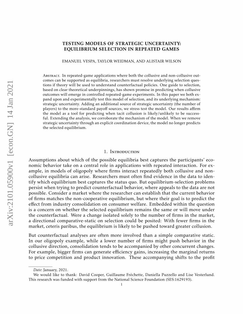
4.1. Main Treatment Differences. The top two lines of Panel (A) in Table 2 report coop-eration rates broken out across the four treatments, where we separately report initial (thefirst round) and ongoing cooperation (all subsequent rounds). The averages in the tableare for the last five supergames—late-session behavior, after subjects have amassed ex-perience in the environment—though including all rounds generates similar results (seeTable A.1 in the Online Appendix). The results point to large cooperation shifts acrossboth the cost to cooperating X and the group size N .

The initial cooperation rate in our(N=2X=$9

)treatment is 50.3 percent, essentially identical

to the 50 percent cooperation rate predicted by the PD meta-study. However, holdingconstant the cooperation cost at X = $9 and doubling the group size to four virtuallyeliminates cooperative behavior, with just 3.5 percent initial cooperation in

(N=4X=$9

). In

29In more detail, our design called for sessions to have at least 20 participants, but allowed us to recruit anadditional group of size N depending on realized show ups. For

(N=10X=$1

)we instead opted to recruit 30 for

each session so that we had at least three groups in each supergame.30All subjects received written and verbal instructions on the task and payoffs, where instructions areprovided for readers in the Online Appendix.31Subjects received full instructions for the first part and were told they would be given instructions onpart two after completing supergame ten. For the four between-subject treatments outlined in section 3,part two was then identical to part one. Later in the paper we will outline a further set of treatments witha within-subject change across the parts. The design choice for two identical parts here allows for directcomparisons in first-half play.32This method is developed in Sherstyuk, Tarui, and Saijo (2013) to induce risk neutrality over supergamelengths. Another benefit from this design choice is that there are no wealth effects within a supergame, andwhere history only matters as an instrument for others’ future play.

17

Table 2. Cooperation rates and basin-effect decomposition

Panel A. Action andsignal rates

X = $9 X = $1

N = 2 N = 4 N = 4 N = 10

Initial coop. 0.503(0.058)

0.035(0.017)

0.792(0.042)

0.357(0.055)

Ongoing coop. 0.450(0.055)

0.006(0.003)

0.409(0.050)

0.184(0.048)

Initial success 0.503 0.000 0.578 0.000Ongoing success 0.450 0.000 0.293 0.000

Panel B. Cooperationdecomposition

p?0 Marginal effect from:

Ind. basin increase to Corr. basin decrease to[0.33] p?0 +∆p?Ind. = [0.69] p?0 −∆p

?Corr. = [0.04]

Initial coop. 0.464(0.058)

−0.395(0.048)

+0.357(0.053)

Ongoing coop. 0.366(0.051)

−0.293(0.051)

+0.115(0.061)

Note: Results are calculated using data from the last-five supergames. Cooperation rates present rawproportions (with subject-clustered standard errors). The cooperation decomposition runs two subject-clustered probits on the cooperation decision (initial and ongoing) where variables are dummies for a lowcorrelated basin treatment (X = $1, both N values) and a high-independent–basin treatment (X = $9/N = 4and X = $1/N = 10). Coefficients shown are the predicted level at just the constant (the p?0 column) and thepredicted cooperation changes from each estimated dummy.

low-temptation settings (X = $1), groups ofN = 4 show highly cooperative behavior (79.2percent for initial decisions), while groups ofN = 10 generate moderate cooperation rates(35.7 percent). The second row of Panel (A) indicates the ongoing (t > 1) cooperation rate.Here the data indicates a decline in cooperation over the initial behavior in all treatments,though the quantitative effects are largest in the $X = 1 treatments.33

The third and fourth rows of Table 2 present the fraction of participant rounds wherea success signal was observed.34 Focusing on success signals, similar patters emerge toongoing cooperation, though with starker quantitative effects. While a success is themodal signal in the

(N=2X=$9

)and

(N=4X=$1

)treatments, in the

(N=4X=$9

)and

(N=10X=$1

)treatments we

observe no successes at all.35

33In the Online Appendix, Table A.2 further breaks out ongoing cooperation by the observed history inthe previous round. The results indicate clear evidence that individual cooperation is highly conditionalon successful coordination. However, strategies are significantly more-forgiving after failed cooperation atX = $1 than X = $9.34A success requires that the other N − 1 participants jointly cooperate. Success is a direct function ofgroup-level cooperation, where the expected success rate with an independent cooperation rate q is qN−1.In two-player games, the success rate is identical to the cooperation rate. For the initial round the expectedsuccess rates (in the Table 2 column order) are: 0.503, 4.2× 10−5, 0.497 and 9.5× 10−5.35As success is a direct aggregate of individual level cooperation we do not report standard errors (wherewe also cannot calculate standard errors when there is no variation). However, the starkness of the effectwith no successes when the independent basin-size is high make clear the underlying economic effects.

18

Using just the raw averages in the top panel of Table 2, the evidence clearly falsifies thecorrelated-basin/null hypothesis on the effect of N , for both initial and ongoing coop-eration. The experimental results indicate large shifts in behavior as we move N as acomparative-static, fixing the value of X. Fixing N = 4 we do find the comparative-staticeffect predicted by the correlated-basin measure as we move X, though this directionaleffect is also predicted by the independent basin.

The evidence suggests that the independent-basin hypothesis fares slightly better. Bothinitial and ongoing cooperation clearly respond in the predicted direction as we shifteither X or N in isolation. However, for initial cooperation, we do not find perfect substi-tution as we move both x and N , as predicted by the independent-basin hypothesis. Thehypothesis predicts no change in cooperation rates comparing either

(N=2X=$9

)to

(N=4X=$1

)or(

N=4X=$9

)to

(N=10X=$1

). When this hypothesis is scrutinized using initial cooperation rates, we

find large differences in either comparison.36 To see this finding from a different perspec-tive, let us pool treatments at each value of X. That is, we compare the average initialcooperation rate pooling

(N=2X=$9

)and

(N=4X=$9

)to the average pooling

(N=4X=$1

)and

(N=10X=$1

). Ini-

tial cooperation in the pooled treatments for X = $9 and X = $1 are 28.6 and 59.4 percent,respectively, and the difference is more than 30 percentage points. In other words, initialcooperation rates are inconsistent with the independent-basin hypothesis.

Results for ongoing cooperation though are substantially better for the independent basin,where

(N=2X=$9

)and

(N=4X=$1

)are not substantially different. We do note a difference between(

N=4X=$9

)and

(N=10X=$1

), this is primarily driven by the very stark finding of near-zero coop-

eration in(N=4X=$9

). We explore this further below. In the aggregate though, pooling the

ongoing cooperation rates across X, we find similar rates at 22.8 percent for X = $9 and29.8 percent for X = $1.

4.2. Evaluation of Independent- and Correlated-Basin Hypotheses. Panel (B) in Table2 provides a direct statistical evaluation of our two competing hypotheses. The table re-ports results of a probit model that assesses subjects’ cooperation decisions using dummyvariables for the 2×2 design in Table 1 Panel (B). The dummy covariates are an indicatorfor the ∆p?Cor. decrease in the correlated basin-size (as we decrease X), and an indicatorfor the ∆p?Ind. increase in the independent basin-size (as we increase N within each X).

Each row in Panel (B) provides the results from a separate estimation, one over initialcooperation, one over ongoing. The first column reports the estimated cooperation ratewhen both dummy variables are zero: essentially the cooperation rate for a game with abasin size of p?0 = 0.33. The final column-pair then report the estimated marginal effecton the cooperation rate for each basin shock, holding the other constant. If either of thetwo basin hypotheses fully explains behavior, we would expect a significant estimate forthe corresponding dummy and an insignificant effect on the other.

36The differences are economically large: 29 percentage points in the first comparison and 35 percentagepoints in the second.

19

(a) Initial cooperation (b) Ongoing cooperation

Figure 2. Cooperation and the Independent Basin-Size ModelNote: Figures show pooled data by the independent basin (diamonds) while the separate treatments areillustrated as the surrounding circles. See Figure A.1 in the appendix for an analogous figure for the corre-lated basin.

The estimation procedure here is designed to directly parallel the probit-model used togenerate predictions from the meta-study. The estimated cooperation rates at p?0 = 0.33is in fact quantitatively very close to the meta-study prediction in Panel (C) of Table 1.Where the meta-study predicts an initial (ongoing) cooperation of 49.5 (37.3) percent,our data at p?0 = 0.33 indicates similar (and statistically inseparable) rates of 46.4 (36.6)percent. To illustrate this, in Figure 2 we provide the fitted relationships from the metastudy but where we overlay results from our four treatments (the smaller circles) usingthe independent basin-size on the horizontal axis. In addition we also indicate the resultspooled over each value for the independent basin measure (the larger diamonds). Whilethere is substantial divergence for initial cooperation in Panel (A), the quantitatively sim-ilar results for ongoing cooperation in Panel (B) are clear.37

Our tests of the two competing hypotheses are focused on the second and third columnsof Panel (B) in Table 2. If the independent (correlated) basin measure captures all rele-vant facets of behavior, we would expect a significantly negative (insignificant) estimatefor the independent-basin increase (correlated-basin-decrease), and an insignificant (sig-nificantly negative) effect on the correlated (independent) basin-increase.

For initial cooperation, we find that changes to both basin-measures generate significanteffects (p < 0.001). The magnitudes of each estimated marginal effect are very similar,

37In Figure A.1 in the Online Appendix we present an analogous figure organized under the correlatedbasin-size model, illustrating much poorer organization of the data, both relatively across the treatmentcomparisons, and quantitatively.

20

though each moving in opposite directions, as predicted. Since neither effect dominates,we conclude that both X and N contain information for predicting initial cooperationthat is not fully absorbed by either basin measure.

However, consistent with our descriptive presentation of the raw treatment rates in Table2 Panel (A), the probit estimates for ongoing cooperation in Panel (B) do break towardsthe independent-basin construction. The coefficient on the increase in the independentbasin is negative and significant (p < 0.001), while the estimate on the decrease for thecorrelated basin is much smaller in magnitude and is not significant at the 5 percentlevel (p = 0.061). Beyond just the qualitative directional effects, the quantitative changein ongoing cooperation under the independent-basin measure is close to the predictedeffects from the relevant basin shifts that we would expect from the RPD meta-studydata. That is, the predicted effect from the meta study for ongoing cooperation when thesize of the basin increases from p?0 = 0.33 to 0.69 is a 21 percentage point drop (see Table1, Panel C), where our estimates indicate a 29 percentage point drop.38

As alluded to above, the differences on ongoing cooperation rates between our data andthe out-of-sample prediction from the meta-study is driven by the stark (essentially bound-ary) behavior in the

(N=4X=$9

)treatment. As illustrated in Figure 1(B) a two-player repeated

game with a a basin of size p? = 0.69 has a predicted ongoing cooperation rate of 16.3 per-cent, where we should be able to reject 11 percent cooperation at 95 percent confidence.While the

(N=10X=$1

)treatment is close to the predicted rate (as are the two other treatments

at p? = 0.33), Figure 1(B) clearly indicates the(N=4X=$9

)treatment being significantly below

the prediction. However, when the non-collusive strategy is risk dominant (when the

independent basin size is greater than12

), the argument made in the literature is that

we should not expect substantial cooperation in this region. Where the model predictslow cooperation at this basin-size, the evidence from Treatment

(N=4X=$9

)pushes towards

this same conclusion, just in a starker way. Aside from the more-extreme coordinationeffects at

(N=4X=$9

), for the other three treatments the theoretically standard extension of

the strategic uncertainty measure comes very close to quantitatively predicting the ongo-ing cooperation level using the out-of-sample relationship estimated from the two-playerRPD meta-data.

We summarize the main findings:

Result 1 (Independent-Basin Measure). The independent-basin measure qualitatively orga-nizes the results for ongoing cooperation, and in all but one treatment matches the quantitativelevel predictions. However, it does not contain all relevant information for predicting initialintentions to collude.

Result 2 (Correlated-Basin Measure). Our data is not consistent with the predictions fromthe correlated-basin hypothesis, neither for initial, nor ongoing cooperation. In particular,

38In contrast, for a decrease to 0.04 we should expect an ongoing cooperation-rate increase of 50 percentagepoints, where we instead we see 11.5 percent.

21

where the correlated basin predicts that behavior should ceteris paribus be unaffected by N weinstead find large cooperation decreases with increases to N .

5. Extensions

Our analysis so far has abstracted away other features of the coordination problem tofocus on the pure effects from the primitives of the strategic game. In this section we con-sider two extensions—with relevance both inside and outside the laboratory—that allowus to study possible limitations of the strategic-uncertainty model to predict changes inequilibrium selection.

First, we consider the extent to which beliefs on others’ collusive behavior may be dis-torted by prior experience. While a policy change can change market primitives and thestrategic-uncertainty measure, the underlying variable in this model is beliefs on others’collusion. It seems plausible that beliefs may be driven by experience before any changein the primitives, and so the model may fare poorly at predicting changes within a pop-ulation. For example, if a player has engaged extensively with the same population ofmarket participants under a status quo that led to non-collusive behavior, their beliefson others acting in this way may be sticky, and therefore unresponsive to shifts in theprimitives that have large effects in the strategic uncertainty model. Our treatments inthe previous section used a between-subjects design. Identification relied on compar-isons of late-session behavior across different populations, each with experience under afixed environment. In a modified treatment pair we examine the effects of varying thenumber of players N within the same population, so that participants have experienceat two distinct values. In this extension we show that outcomes do not exhibit long-runstickiness, where the between-subject results detailed previously are not substantiallydissimilar when we examine them within-subject.

In a second set of extensions, we examine the strategic uncertainty mechanism under-lying the basin-size selection device. In particular we examine the extent to which ourresults are affected by the possibility of explicit coordination, holding constant X and N .Here we seek to mirror an empirical finding that when collusion in industries is detected,it is often accompanied by evidence of explicit collusion—despite the illegality of suchmeetings.39 In one treatment we show that once explicit collusion is allowed for, neitherthe independent nor the correlated basin measures does a good job of predicting collusivebehavior levels. Once parties can explicitly collude we find very high levels of sustainedcooperation. This suggests that indeed uncertainty over the other strategic choices is amain driver of behavior in our main treatments. However, the extremeness of the ef-fect once communication is allowed for raises a question over the extent to which explicitcollusion might lead to high cooperation rates even when collusive outcomes are not equi-librium. To examine this, we show that there a clear limits on what explicit collusion canachieve is defined by the theoretical existence of collusive equilibria.

5.1. Between vs. Within Identification. The motivating idea for our first extension isthat in many settings of interest the policy-relevant comparative static is being varied

39See Marshall and Marx (2012) for a more comprehensive treatment.22

within a population. However, if agents have strong beliefs about others due to prior ex-periences, it may be that our theoretical construction lacks bite at predicting outcomes asthe policy shifts. If selected equilibria are very sticky within a population, then more-standard assumptions maintaining the equilibria across the counterfactual may havegreater validity. For example, within the experiment if a participant’s experience withothers is that they play the stage-game defection action every period, then this belief canpersist despite a policy shift that makes collusion easier.

Ideally, we would introduce a primitive change within a supergame—for example, a movefrom N = 4 to N = 2, where the matched player after the modification is one of thematched participants from before. In exploring potential designs for this, we were notsatisfied that they would produce clear results. First, it is well-documented that repeated-game environments require several supergames of experience for participants to inter-nalize the environment (Dal Bó, 2005). While implementing a surprise change in N asa mid-supergame manipulation would mirror an outside-the-laboratory consolidation,this would provide a single supergame observation, and require substantial explanationacross the surprise. An alternative design choice could implement a change in N withsome probability within each supergame. However, any observed effects would then beconfounded with the expectations over the primitive change (and greater complication inthe instructions) and would no longer comparable to our between-subject treatments.

Given the potential confounds with other designs we instead opted—certainly as a firstapproach— for a design with a surprise one-time shift in the number of players N , butwhere this occurred in a fixed session-level population. Holding constant the cooper-ation cost at X = $9, we initially set a value of N (either two or four) for the first tensupergames. We then change the value of N for the last ten supergames (to either four ortwo, respectively).

This led to two further experimental treatments, one with(N=2X=$9

)in the first half, and(

N=4X=$9

)in the second; and the converse treatment from

(N=4X=$9

)in the first, to

(N=2X=$9

)in the

second half. In both treatments, the change inN comes as a surprise: subjects know thereis a second part, but do not receive instructions on it until supergame ten concludes.40 Interms of the standard strategic-uncertainty model this creates a shift across the sessionfrom a low basin-size of 0.33 when N = 2, and a high basin-size of 0.69 when N = 4.In particular, this is a change in N where our between-subject design indicates a sub-stantial treatment effect. Given that we hold constant X = $9, for simplicity we label thetreatments as 2→ 4 and 4→ 2, for the first-half to second-half shifts.

In Figure 3(A) we present the average initial cooperation-rates across the session’s twentysupergames. The between-subject treatments with N = 2 and N = 4 are indicated by thetwo gray dashed lines (separately labeled), while the within-subject treatment results arerepresented by two black lines: a solid line for the 2→ 4 treatment, and a dash-dotted-line for the 4→ 2 treatment. The figure illustrates the substantial between-subject effect,with more cooperation in

(X=$9N=2

)over

(X=$9N=4

)for all twenty supergames. Our within and

40Our between-subject treatments also divided the session into two parts, except that once subjects reachedthe second half of the session they were told that part two was identical to part one.

23

between sessions are identical for the first ten supergames, where the figure indicatesreplicated effects. Pooling the between and within treatments with N = 2 in supergames6–10 the initial cooperation rate is 47.4 percent. In contrast, the pooled cooperation ratefor N = 4 is just 13.9 percent.41

As we move into supergames 11–20, the number of players matched in each supergamechanges for our within treatments. Figure 3(A) indicates the immediate shift in behavioras the primitive changes as the two vertical dotted lines. For the 2 → 4 treatment (theblack solid line) initial cooperation levels remain fairly high after the shift from N = 2to N = 4. In fact, cooperation in the first four-player interaction (supergame 11) actuallyexhibits an increase to 59.7 percent from the 53.0 percent from the last two-player inter-action (supergame 10). However, while there is no immediate cooperation drop-off, andthus stickiness, as subjects gain experience at N = 4 the cooperation rate falls rapidly,reaching 16.7 percent by supergame 20. In contrast, moving in the other direction fromN = 4 to N = 2 (the black dash-dot line) we find an immediate jump with the primitiveshift. Where initial-round cooperation in supergame 10 with four-players is 18.3 percent,the reduction to N = 2 pushes this rate up to 60.0 percent for supergame 11. The im-mediate jump in behavior is then sustained across the remaining supergames, with 58.3percent cooperation in supergame 20.

Inspecting the session time-series illustrated in Figure 3(A) it is clear that the there is littleevidence for the hypothesis that equilibrium selection is sticky in the long-run under awithin-population shift in N . Despite exposure to the alternative environment in thefirst half, longer-run behavior in the second-half is not substantially dissimilar from thebetween-subject levels. This is indicated by the close proximity of the two black/gray linepairs at supergame 20, and relative distance from the other pair.

In Online Appendix B we provide a more detailed like-with-like comparison of the between-subject and within-subject results. These more-detailed findings indicate no differencewith the between-subject results as we move from 2→ 4. However, in opposition to thehypothesis that the selected equilibrium is sticky, we actually find a significant increasesin the response to N over the between analysis as we move from 4→ 2. We summarizethe result:

Result 3 (Between vs. Within). Switching the identification to within does not substantiallychange our qualitative results, finding no evidence that the selected equilibrium is sticky inthe long run as we shift a primitive within the population. If anything, our within-subjectidentification shows a larger shift than the between-subject results as we decrease N .

5.2. Explicit Correlation. The focus so far, and for the RPD literature more generally,is an examination of implicit coordination. Our results thus far suggest that a model ofstrategic uncertainty extended via independence is relatively successful at organizing thedata. This is particularly so for ongoing cooperation. In contrast, a measure based on

41Testing the initial cooperation rate differences in supergames 6–10 over N (so across the between andwithin sessions with identical treatment at this point) we find p = 0.150 for N = 2 and p = 0.981 for N = 4from t-tests for a level difference, and p = 0.353 for a joint test.

24

(a) Between vs. Within (X = $9) (b) Explicit vs. Implicit ((N=4X=$9

))

Figure 3. Initial cooperation rates in extensions (by supergame)

perfectly correlated play fails to predict the substantial effect of N for both initial andongoing behavior.

These results are therefore a validation of a standard extension of the basin of attractionnotion. However, correlation across participants’ beliefs becomes much more plausiblewhen participants have access to a channel through which to explicitly coordinate. Inan extension to our previous experiments we now examine the extent to which multipleparties successfully collude when given a coordination device.

To this end, we designed a further treatment pair that modifies our environment withthe starkest coordination on the non-collusive outcome, the

(N=4X=$9

)treatment. In the first

chat treatment, the first 10 supergames were identical to the(N=4X=$9

)treatment, but we

introduce pre-supergame chat between the four matched players in supergames 11–20. Asecond chat treatment is identical to the first in terms of the timing for when we introducethe chat coordination device; the difference is that we reduce the continuation probabilityto δ′ = 1/2 for the entire session. The designed effect of this change is that while the stage-game payoffs and number of players is held constant, at this value of δ the grim trigger isnow only a knife-edge SPE, where the critical belief p?(δ′) = 1 under both (2) and (3). The

δ =12

treatment therefore serves as a test for whether explicit coordination can implement

outcomes that are not supportable as a robust equilibrium (that is, with arbitrarily smalltrembles in behavior).

In an online supplement we provide chat logs for the interested reader; however, we herefocus on the of effects of chat on cooperation levels. In Figure 3(B) we plot the average

25

Table 3. Cooperation: Implicit vs. Explicit

Implicit Explicit

NoChat(3/4) Chat(3/4) Chat(1/2)

Initial coop. 0.035(0.017)

0.988(0.007)

0.300(0.037)

Ongoing coop. 0.006(0.003)

0.806(0.030)

0.044(0.018)

Initial success 0.000 0.971 0.094Ongoing success 0.000 0.756 0.002

Note: All treatments have x = $9,N = 4, where NoChat(3/4) is from the core 2 × 2 between-subject designoutline in section 4. Data taken from last five supergames, participant-clustered standard errors in paren-theses.

initial cooperation rates across sessions (with the(N=4x=$9

)treatment provided as a base-

line, labeled here as NoChat(3/4)). Late-session cooperation and success rates (assessed insupergames 16–20 with subject-clustered standard errors) are provided in Table 3.

Our first chat treatment delivers unequivocal results: providing pre-play communica-tion at δ = 3/4 takes the near-zero cooperation rate in the absence of chat to almost com-plete cooperation. While ongoing cooperation drops slightly from the very high initial-cooperation levels, the large majority of supergames exhibit coordination by all four par-ticipants on the efficient/collusive outcome. Such high levels of cooperation with com-munication are inconsistent with the predictions of either model of equilibrium selectionfor these primitives. This suggests that once explicit coordination devices are allowedfor and strategic uncertainty is reduced, the independent model–that captured behaviorwhen collusion is tacit–is no longer helpful.

However, at the δ = 1/2 boundary for dynamic strategies to be incentive compatible, evenwith pre-play communication participants find it hard to coordinate. While initial coop-eration levels are substantially higher than the treatment without chat at 30.0 percent,ongoing cooperation falls to just 4.4 percent, where successful joint-cooperation acrossan entire group in an ongoing round becomes exceedingly rare at 0.2 percent. The find-ings therefore indicate that for explicit communication to play a role, clear incentives forcollusion do need to be present.

Given the very stark findings here, we simply summarize the extension result:

Result 4 (Implicit vs. Explicit). Explicit coordination leads to very high cooperation levelswith multiple players, in a setting where implicit cooperation achieves near-zero cooperation.However, in the limiting case, where cooperation is a knife-edge SPE outcome, even pre-playchat fails to support cooperation in our experiments.

26

6. Conclusion

Our paper examines equilibrium selection in repeated games, and the extent to which itcan be predicted with a model of strategic uncertainty. We leverage a model of equilib-rium selection that rationalizes behavior in data from repeated prisoner’s dilemma (RPD)experiments and design an experiment to stress test this specific theoretical model. Thepredictive model works by mediating the effects from multiple-primitives into a singledimension, strategic uncertainty. As such, even for rich counterfactual policies with manychanges to the setting, the model can still generate a directional prediction. The exper-imental design builds on this motivation for the model, introducing a novel source ofstrategic uncertainty that has not been studied in the RPD setting (the number of play-ers) while also manipulating a payoff parameter. We can thus change both sources ofstrategic uncertainty simultaneously and study the extent to which the evidence is con-sistent with the predictions of the selection model. Our main finding is that the model ofequilibrium selection can indeed be used as a device for understanding successful coor-dination on the collusive outcome. In particular, the model performs well in trading-offthe competing effects from the two distinct sources of strategic uncertainty.

After illustrating the theoretical power of the model for implicit coordination, we turnour attention to two application-motivated extensions that probe its limitations. In thefirst, we are motivated by the extent to which prior history and experience could makethe equilibria “sticky,” even where the model suggests a change. To do this, we studythe extent to which our findings still hold when treatment-variable manipulations takesplace within the same population, as opposed to between populations in our main study.The results indicate that eve when the participants experience a treatment-variable shift,the model still continues to predict the longer run outcomes. While we do find somehysteresis in the short-run response to a within-population policy change—initial stick-iness in behavior in one direction and a large immediate response to the change in theother—behavior after some experience under the new parameters is not distinct from thebetween-population treatments. As such, while a plausible limitation of the model wasthe effect of prior experience, these results suggest that the model prediction fares betterthan the more-standard assumption of maintaining a selected equilibrium across a policychange.

Finally, in a second extension, we examine the potential effects from explicit collusion.Shifting the experimental environment by providing an explicit coordination device (pre-play chat) we examine a necessary limitation on the model if the underlying strategic un-certainty mechanism is correct. Our main finding here is that once we allow for explicitcoordination then the selection-model prediction is very far from observed behavior. Infact, where the model suggests very low levels of cooperation, actual behavior is at theother extreme once coordination devices are present. The evidence from the second ex-tension therefore indicates both that strategic uncertainty plays a clear role, but also thatthe selection model based upon it is entirely inappropriate for predicting behavior whenexplicit collusion is suspected.

Though our results are encouraging, for the theoretical selection model we examine tobe useful in applications further tests are needed. First, as we point out when describing

27

our experimental design, there are many ways in which expanding the multiple playersmight impact the game.Because we do not want to introduce further coordination issues,we focus on a setting where collusion requires joint cooperation form all of the agents.But in other interesting environments cooperation among a subset of the agents may beenough for reaching an efficient outcome. Such environments introduce further distribu-tional coordination problems, over who cooperates and who free-rides. Further researchis needed to evaluate how and if models of equilibrium selection might be extended tosuch problems. Outside from the role of multiple players, there are also outstandingquestions with regard to how asymmetries for the players—in terms of actions, payoffs,and the sequentiality of moves—should be modeled.

From another perspective, our results also outline that there is room to evaluate the rolefor equilibrium selection model in environments with explicit collusion. Our findingssuggest one clear limit on where explicit collusion can play a role: the existence of a col-lusive equilibrium. However, beyond this point, not much is known about the conditionsfor which explicit communication between the parties is enough for collusion. Anotherdirection for future research is to try to understand if there are ways to manipulate theprimitives to understand when explicit collusion will and will not be successful.

References

Agranov, Marina, Guillaume Frechette, Thomas Palfrey, and Emanuel Vespa (2016),“Static and dynamic underinvestment: An experimental investigation.” Journal of Pub-lic Economics, 143, 125–141.

Battaglini, Marco, Salvatore Nunnari, and Thomas R Palfrey (2012), “Legislative bargain-ing and the dynamics of public investment.” American Political Science Review, 106,407–429.

Battaglini, Marco, Salvatore Nunnari, and Thomas R Palfrey (2016), “The dynamic freerider problem: A laboratory study.” American Economic Journal: Microeconomics, 8, 268–308.

Battalio, Raymond, Larry Samuelson, and John Van Huyck (2001), “Optimization incen-tives and coordination failure in laboratory stag hunt games.” Econometrica, 69, 749–764.

Berry, James, Lucas C Coffman, Douglas Hanley, Rania Gihleb, and Alistair J Wilson(2017), “Assessing the rate of replication in economics.” American Economic Review,107, 27–31.

Blonski, Matthias and Giancarlo Spagnolo (2015), “Prisoners’ other dilemma.” Interna-tional Journal of Game Theory, 44, 61–81.

Brandts, Jordi and David J Cooper (2006), “A change would do you good.... an exper-imental study on how to overcome coordination failure in organizations.” AmericanEconomic Review, 96, 669–693.

Cason, Timothy N. (2008), “Price signaling and ‘cheap talk’ in laboratory posted offermarkets.” Handbook of Experimental Economics Results, 1, 164–169.

28

Cason, Timothy N., Tridib Sharma, and Radovan Vadovič (2020), “Correlated beliefs:Predicting outcomes in 2× 2 games.” Games & Economic Behavior, 122, 256–276.

Compte, Olivier, Frederic Jenny, and Patrick Rey (2002), “Capacity constraints, mergersand collusion.” European Economic Review, 46, 1–29.

Cooper, David J. and Kai-Uwe Kühn (2014), “Communication, renegotiation, and thescope for collusion.” American Economic Journal: Microeconomics, 6, 247–78.

Dal Bó, Pedro (2005), “Cooperation under the shadow of the future: experimental evi-dence from infinitely repeated games.” American Economic Review, 95, 1591–1604.

Dal Bó, Pedro and Guillaume R Fréchette (2011), “The evolution of cooperation in infin-itely repeated games: Experimental evidence.” American Economic Review, 101, 411–429.

Dal Bó, Pedro and Guillaume R Fréchette (2018), “On the determinants of cooperation ininfinitely repeated games: A survey.” Journal of Economic Literature, 56, 60–114.

Davis, Douglas D (2002), “Strategic interactions, market information and predicting theeffects of mergers in differentiated product markets.” International Journal of IndustrialOrganization, 20, 1277–1312.

Deneckere, Raymond and Carl Davidson (1985), “Incentives to form coalitions withbertrand competition.” RAND Journal of Economics, 473–486.

Devetag, Giovanna and Andreas Ortmann (2007), “When and why? a critical survey oncoordination failure in the laboratory.” Experimental economics, 10, 331–344.

Dufwenberg, Martin and Uri Gneezy (2000), “Price competition and market concentra-tion: an experimental study.” International Journal of Industrial Organization, 18, 7–22.

Farrell, Joseph and Carl Shapiro (1990), “Horizontal mergers: an equilibrium analysis.”American Economic Review, 107–126.

Fonseca, Miguel A and Hans-Theo Normann (2012), “Explicit vs. tacit collusion—theimpact of communication in oligopoly experiments.” European Economic Review, 56,1759–1772.

Fréchette, Guillaume, Alessandro Lizzeri, and Emanuel Vespa (2020), “Collusion in mul-timarkets: An experiment.” NYU Working Paper.

Fudenberg, D., D.G. Rand, and A. Dreber (2010), “Slow to anger and fast to forgive:Cooperation in an uncertain world.” American Economic Review.

Ghidoni, Riccardo and Sigrid Suetens (forthcoming), “The effect of sequentiality on co-operation in repeated games.” American Economic Journal: Microeconomics.

Goette, Lorenz and Armin Schmutzler (2009), “Merger policy: What can we learn fromcompetition policy.” Experiments and Competition Policy; Hinloopen, J., Normann, HT,Eds, 185–216.

29

Harrington, Joseph E, Roberto Hernan Gonzalez, and Praveen Kujal (2013), “The relativeefficacy of price announcements and express communication for collusion: Experimen-tal findings.” Working paper. University of Pennsylvania, The Wharton School.

Harrington, Joseph E, Roberto Hernan Gonzalez, and Praveen Kujal (2016), “The relativeefficacy of price announcements and express communication for collusion: Experimen-tal findings.” Journal of Economic Behavior & Organization, 128, 251–264.

Harsanyi, John C and Reinhard Selten (1988), A general theory of equilibrium selection ingames. MIT Press, Cambridge, MA.

Horstmann, Niklas, Jan Krämer, and Daniel Schnurr (2018), “Number effects and tacitcollusion in experimental oligopolies.” Journal of Industrial Economics, 66, 650–700.

Huck, Steffen, Kai A. Konrad, Wieland Müller, and Hans-Theo Normann (2007), “Themerger paradox and why aspiration levels let it fail in the laboratory.” Economic Journal,117, 1073–1095.

Huck, Steffen, Hans-Theo Normann, and Jörg Oechssler (2004), “Two are few and fourare many: number effects in experimental oligopolies.” Journal of Economic Behavior &Organization, 53, 435–446.

Kartal, Melis and Wieland Müller (2018), “A new approach to the analysis of cooperationunder the shadow of the future: Theory and experimental evidence.” University ofVienna working paper.

Kartal, Melis, Wieland Müller, and James Tremewan (2017), “Building trust: The costsand benefits of gradualism.” University of Vienna working paper.

Kloosterman, Andrew (2019), “Cooperation in stochastic games: a prisoner’s dilemmaexperiment.” Experimental Economics, 1–21.

Lugovskyy, Volodymyr, Daniela Puzzello, Andrea Sorensen, James Walker, and Arling-ton Williams (2017), “An experimental study of finitely and infinitely repeated linearpublic goods games.” Games & Economic Behavior, 102, 286–302.

Marshall, Robert C and Leslie M Marx (2012), The economics of collusion: Cartels andbidding rings. MIT Press.

Perry, Martin K and Robert H Porter (1985), “Oligopoly and the incentive for horizontalmerger.” American Economic Review, 75, 219–227.

Potters, Jan and Sigrid Suetens (2013), “Oligopoly experiments in the current millen-nium.” Journal of Economic Surveys, 27, 439–460.

Rosokha, Yaroslav and Chen Wei (2020), “Cooperation in queueing systems.” WorkingPaper.

Salz, Tobias and Emanuel Vespa (2020), “Estimating dynamic games of oligopolistic com-petition: An experimental investigation.” RAND Journal of Economics, 51, 447–469.

Sherstyuk, Katerina, Nori Tarui, and Tatsuyoshi Saijo (2013), “Payment schemes ininfinite-horizon experimental games.” Experimental Economics, 16, 125–153.

30

Vespa, Emanuel (2020), “An experimental investigation of cooperation in the dynamiccommon pool game.” International Economic Review, 61, 417–440.

Vespa, Emanuel and Alistair J Wilson (2019), “Experimenting with the transition rule indynamic games.” Quantitative Economics, 10, 1825–1849.

Vespa, Emanuel and Alistair J Wilson (2020), “Experimenting with equilibrium selectionin dynamic games.” Working Paper.

Vesterlund, Lise (2016), “Using experimental methods to understand why and how wegive to charity.” Handbook of Experimental Economics, 2, 91–151.

Weber, Roberto A (2006), “Managing growth to achieve efficient coordination in largegroups.” American Economic Review, 96, 114–126.

Wilson, Alistair J. and Emanuel Vespa (2020), “Information transmission under theshadow of the future: An experiment.” American Economic Journal: Microeconomics,12.

31

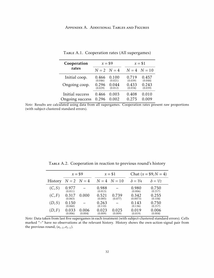
Appendix A. Additional Tables and Figures

Table A.1. Cooperation rates (All supergames)

Cooperationrates

x = $9 x = $1

N = 2 N = 4 N = 4 N = 10

Initial coop. 0.466(0.046)

0.100(0.021)

0.719(0.039)

0.457(0.044)

Ongoing coop. 0.296(0.029)

0.044(0.012)

0.433(0.034)

0.243(0.039)

Initial success 0.466 0.003 0.408 0.010Ongoing success 0.296 0.002 0.275 0.009

Note: Results are calculated using data from all supergames. Cooperation rates present raw proportions(with subject-clustered standard errors).

Table A.2. Cooperation in reaction to previous round’s history

x = $9 x = $1 Chat (x = $9,N = 4)

History N = 2 N = 4 N = 4 N = 10 δ = 3/4 δ = 1/2

(C,S) 0.977(0.011)

– 0.988(0.013)

– 0.980(0.006)

0.750(0.217)

(C,F) 0.317(0.063)

0.000 0.521(0.085)

0.739(0.077)

0.342(0.0073)

0.255(0.104)

(D,S) 0.150(0.060)

– 0.263(0.110)

– 0.143(0.136)

0.750(0.217)

(D,F) 0.033(0.006)

0.006(0.004)

0.023(0.009)

0.025(0.009)

0.019(0.019)

0.006(0.004)

Note: Data taken from last five supergames in each treatment (with subject-clustered standard errors). Cellsmarked “–” have no observations at the relevant history. History shows the own-action-signal pair fromthe previous round, (at−1,σt−1).

32

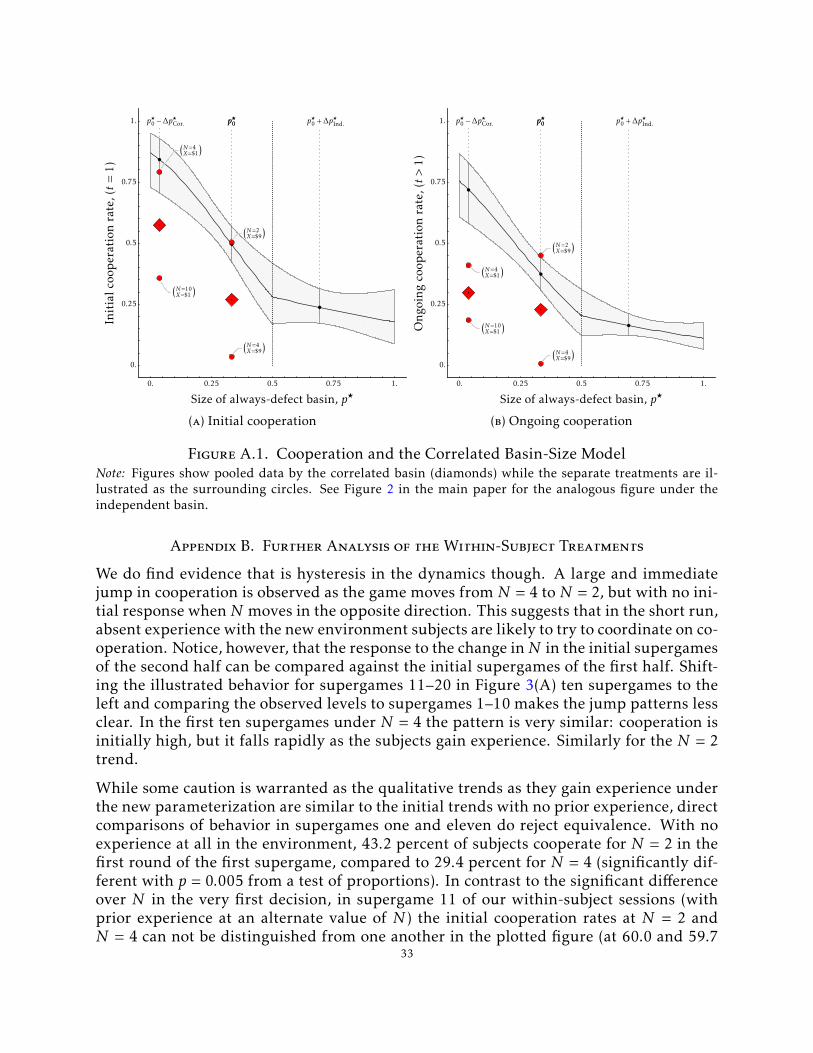
(a) Initial cooperation (b) Ongoing cooperation

Figure A.1. Cooperation and the Correlated Basin-Size ModelNote: Figures show pooled data by the correlated basin (diamonds) while the separate treatments are il-lustrated as the surrounding circles. See Figure 2 in the main paper for the analogous figure under theindependent basin.

Appendix B. Further Analysis of the Within-Subject Treatments

We do find evidence that is hysteresis in the dynamics though. A large and immediatejump in cooperation is observed as the game moves from N = 4 to N = 2, but with no ini-tial response whenN moves in the opposite direction. This suggests that in the short run,absent experience with the new environment subjects are likely to try to coordinate on co-operation. Notice, however, that the response to the change inN in the initial supergamesof the second half can be compared against the initial supergames of the first half. Shift-ing the illustrated behavior for supergames 11–20 in Figure 3(A) ten supergames to theleft and comparing the observed levels to supergames 1–10 makes the jump patterns lessclear. In the first ten supergames under N = 4 the pattern is very similar: cooperation isinitially high, but it falls rapidly as the subjects gain experience. Similarly for the N = 2trend.

While some caution is warranted as the qualitative trends as they gain experience underthe new parameterization are similar to the initial trends with no prior experience, directcomparisons of behavior in supergames one and eleven do reject equivalence. With noexperience at all in the environment, 43.2 percent of subjects cooperate for N = 2 in thefirst round of the first supergame, compared to 29.4 percent for N = 4 (significantly dif-ferent with p = 0.005 from a test of proportions). In contrast to the significant differenceover N in the very first decision, in supergame 11 of our within-subject sessions (withprior experience at an alternate value of N ) the initial cooperation rates at N = 2 andN = 4 can not be distinguished from one another in the plotted figure (at 60.0 and 59.7

33

Table A.3. Cooperation: Between vs. Within

Between (SG 6–10) Within (SG 16–20) ∆Btwn. ∆Wthn.

N = 2 N = 4 N = 2 N = 4 2→ 4 4→ 2

Initial coop. 0.474(0.036)

0.139(0.025)

0.643(0.056)

0.214(0.041)

−0.469(0.060)

−0.260(0.042)

−0.504(0.056)

Ongoing coop. 0.299(0.026)

0.054(0.012)

0.598(0.051)

0.042(0.016)

−0.444(0.055)

−0.258(0.029)

−0.544(0.050)

Initial success 0.474 0.011 0.643 0.042 -0.503 -0.433 -0.632Ongoing success 0.299 0.004 0.598 0.008 -0.450 -0.292 -0.594

Note: Comparisons at the same experience level are generated using supergames 6–10 across all sessions(fixing N , between and within sessions are identical until supergame 11). For the within change we mea-sure the cooperation rates in supergames 16–20. All cooperation rates are raw proportions (with subject-clustered standard errors). The last three columns measure the corresponding cooperation rate whenN = 4minus the cooperation rate when N = 2.

percent cooperation, respectively), let alone statistically (p = 0.974). Both cooperationrates are significantly greater than the initial responses in supergame one.42 We concludethat experience at another parameter value in the first half does cause both treatments’cooperation rates to increase.

In Table A.3 we provide more details, where we compare and contrast the behavior af-ter 5 rounds of experience. In the first two data columns we present average behavior(initial/ongoing cooperation and success, with subject-clustered standard errors for theindividual choices) in supergames 6–10 for N = 2, N = 4. In the next column pair wepresent the same information in supergames 16–20 for the within treatments only. Ex-amining the differences across the within and between cooperation levels, while we find nosignificant differences in behavior for N = 4 (p = 0.117/p = 0.539 for initial/ongoing co-operation) we do find significant differences across the N = 2 cooperation rates (p = 0.011for initial, p < 0.001 for ongoing). The significant differences here reflect the substantiallygreater upward shift in the 4→ 2 treatment.

In the final three columns, we compute (for three different cases) the average cooperationrate in supergames when N = 4 minus the cooperation rate when N = 2. In the firstcolumn (∆Btwn) we calculate the between-subject change using data from supergames16–20 in the X = $9 between-subject treatments. The results here are analogous to themarginal effect attributable to an increase in the independent basin of ∆p?Ind. = +0.36 inTable 2 once we remove the X = $1 treatments. In the final column pair we present thesame assessed treatment effect if we used the within-subject difference in the 2→ 4 and4→ 2 treatments (here we compare data in supergames 6–10 to supergames 16–20).

While the three measures agree qualitatively—and exhibit economically large effects inNin the same direction—there are differences, particularly in the comparisons to the 2→ 4

42Given the disjoint subject groups and identical treatment in supergames 1–10, we compare proportionsusing t-tests without clustering. We then compare the initial response under each value of N in the within-subject supergame eleven to all subjects at thatN in supergame one. Using these tests we reject equivalencewith p = 0.021 for N = 2 and p < 0.001 for N = 4.

34

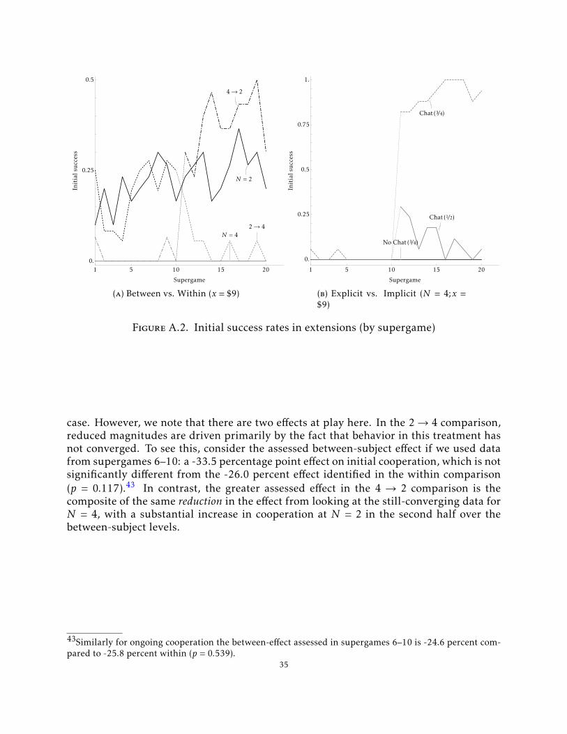
(a) Between vs. Within (x = $9) (b) Explicit vs. Implicit (N = 4;x =$9)

Figure A.2. Initial success rates in extensions (by supergame)

case. However, we note that there are two effects at play here. In the 2→ 4 comparison,reduced magnitudes are driven primarily by the fact that behavior in this treatment hasnot converged. To see this, consider the assessed between-subject effect if we used datafrom supergames 6–10: a -33.5 percentage point effect on initial cooperation, which is notsignificantly different from the -26.0 percent effect identified in the within comparison(p = 0.117).43 In contrast, the greater assessed effect in the 4 → 2 comparison is thecomposite of the same reduction in the effect from looking at the still-converging data forN = 4, with a substantial increase in cooperation at N = 2 in the second half over thebetween-subject levels.

43Similarly for ongoing cooperation the between-effect assessed in supergames 6–10 is -24.6 percent com-pared to -25.8 percent within (p = 0.539).

35

Appendix C. Interface Screenshots

(a) Action Selection

(b) Round Feedback

(c) Supergame Feedback

Figure A.3. Interface Screenshots

36

Appendix D. Provided Instructions

Below we include the instructions given to participants. All language deltas/treatment-specific language are included in braces. Text in red is for the N = 2 treatment, in bluefor the N > 2 treatments (here we provide the N = 4 implementation, where N = 10has only minor changes.). In green we provide the payoff text for X = $9, in orange forX = $1. Separate instructions for {Part two} are given by treatment for the extensions.The only unlisted treatment variation here is for the Chat(1/2) treatment, where the onlychanges are for the critical die rolls in the Study Organization & Payment section, wherethe supergame cutoff changes from 75 to 50.

37

Instructions

Welcome. You are about to participate in a study on decision-making. What you earndepends on your decisions, and the decisions of others in this room. Please turn off yourcell phones and any similar devices now. Please do not talk or in any way try to com-municate with other participants. We will start with a brief instruction period. Duringthe instruction period you will be given a description of the main features of the study.If you have any questions during this period, raise your hand and your question will beanswered in private at your computer carrel.

Study Organization & Payment.

• The study has two Parts, where each Part has 10 decision-making Cycles. EachCycle consists of a random number of Rounds where you make decisions.

• At the end of the study, one of the two Parts will be selected for payment withequal probability. For the selected Part, one of the 10 Cycles will be randomlyselected for payment. Your payment for this randomly selected Cycle will be basedon your decision’s in that Cycle’s last Round.

• The number of Rounds in each Cycle is random, where only the last Round in eachCycle counts for payment. Which Round is the last is determined as follows:

– In every Round, after participants make their decisions, the computer willroll a fair 100-sided die. If the die roll is greater than 75 (so 76–100) theround just completed is the one that is used to determine the current Cycle’spayment, and the Cycle ends. If instead the computer’s roll is less than 75 (so1– 75) then the Cycle continues into another Round.

– Because of this rule, after every Round decision there is a 25 percent chancethat the current Round is the ones that count for the Cycle’s payment, and a75 percent chance that the Cycle continues and the decisions in a subsequentround will count for that Cycle payment.

• Your final payment for the study will be made up of a $6 show-up fee, and yourpayment from the last Round in the randomly selected Cycle.

Part 1.

• In the first part of the study you will make decisions in 10 Cycles. In each Cy-cle you will be matched with {another participant}{a group of three other partic-ipants} in the room for a sequence of Rounds. You will interact with the same{other participant}{group of three other participants} in all rounds of the cycle.

• Once a Cycle is completed, you will be randomly matched to a new {partici-pant}{group of three participants} for the next Cycle.

• While the specific {participant}{participants} you are matched to is fixed across allRounds in the Cycle, the computer interface in which you make your decisions

38

is anonymous, so you will never find out which participants in the room you in-teracted with in a particular Cycle, nor will others be able to find out that theyinteracted with you.

Round Choices and Payoffs. For each Round in each Cycle, you and the matched {par-ticipant}{participants in your group} will make simultaneous choices. {Both}{All four} ofyou must choose between either the Green action or the Red action. After you and theother {participant}{three participants} have made your choices, you will be given feed-back on the {other participant’s}{other participants’} choices that Round, alongside theComputer’s die roll to determine if that Round counts for the Cycle payment.

If a particular Round is the Cycle’s last, and that Cycle is the one selected for final pay-ment, there are four possible payoff outcomes.

(i) If both you and {the other participant}{all three of the other participants} choosethe Green action, you get a round payoff of $20.

(ii) If you choose the Green action and {the other participant chooses}{any of the otherparticipants choose} Red, you get a round payoff of {$2}{$10}.

(iii) If you choose the Red action and {the other participant chooses}{all of the threeother participants choose} Green, you get a round payoff of {$29}{$21}.

(iv) If both you and {the other participant}{any of the other three participants} choosethe Red action, you get a round payoff of $11.

These four payoffs are summarized in the following table:

Other {Participant’s Action:}{Participants’ Actions:}{Green}{All 3 Green} {Red}{Any of 3 Red}

Your Action: Green $20 {$2}{$10}Red {$29}{$21} $11

Some examples of these payoffs:

Case 1. Suppose you choose Green and {the other participant}{all three of the other par-ticipants} in the Cycle also choose Green. If that Round is the final one in the Cycle{both}{all four} of you would get a payoff of $20.

Case 2. Suppose {you}{you and two of the other participants} choose Green while theother participant chooses Red. If that Round is the final one in the Cycle {you}{you andthe other two participants who chose Green} would get a payoff of {$2}{$10}, while theother participant would get a payoff of {$29}{$21}.

Case 3. Suppose you chooseRed while {the other participant chooses}{all three of theother participants choose} Green. If that Round is the final one in the Cycle you wouldget a payoff of {$29}{$21}, while the other {participant}{three participants} would get apayoff of {$2}{$10}.

Case 4. Suppose you and {the other participant choose Red.}{another participant chooseRed while the other two participants choose Green.} If that Round is the final one in the

39

Cycle {you}{you and the other participant that chose Red} would get a payoff of {$11}{$11,while the other two participants would get a payoff of{$2}{$10}} .

Part 2. After Part 1 is concluded, you will be given instructions on Part 2, which will havea very similar structure to the task in Part 1.

{END OF PART 1 HANDOUT}

Part 2 Instructions {Between Only, handed out Supergame 11}. Part 2 is identical toPart 1. In each of the 10 Cycles in Part 2 you will again be matched to {another partici-pant}{three other participants} in the room.

Similar to Part 1, the Cycle payoff is determined by the last round in the Cycle, where thepayoff depends on the action you chose and the {action chosen by the matched partici-pant}{actions chosen by the three matched participants} for that Cycle. Similar to Part 1,the below Table summarizes the payoff based upon the choices made in the Cycle’s lastround.

Other {Participant’s Action:}{Participants’ Actions:}{Green}{All 3 Green} {Red}{Any of 3 Red}

Your Action: Green $20 {$2}{$10}Red {$29}{$21} $11

{END OF PART 2 HANDOUT}

Part 2 Instructions {Within Only, handed out Supergame 11}. Part 2 is very similar toPart 1. However, in each of the 10 Cycles in Part 2 you will instead be matched to threeother participants in the room for each Cycle.

Similar to Part 1, the Cycle payoff is determined by the last round in the Cycle, wherethe payoff depends on the action you chose and the actions chosen by the three matchedparticipants for that Cycle. If a particular Round is the Cycle’s last, and that Cycle is theone selected for final payment, there are four possible payoff outcomes.

(i) If both you and all three of the other participants choose the Green action, you geta round payoff of $20.

(ii) If you choose the Green action and any of the other participants chooses Red, youget a round payoff of $2.

(iii) If you choose the Red action and all three other participants choose Green, youget a round payoff of $29.

(iv) If both you and any of the other three participants choose the Red action, you geta round payoff of $11.

These four payoffs are summarized in the following table:

Other Participant’s Action:All 3 Green Any of 3 Red

Your Action: Green $20 $2Red $29 $11

40

Some examples of these payoffs:

Case 1. Suppose you choose Green and all three of the other participants in the Cyclealso choose Green. If that Round is the final one in the Cycle all four of you would get apayoff of $20.

Case 2. Suppose you and two of the other participants choose Green while the otherparticipant chooses Red. If that Round is the final one in the Cycle you and the other twoparticipants who chose Green would get a payoff of $2, while the other participant wouldget a payoff of $29.

Case 3. Suppose you choose Red while all three of the other participants choose Green.If that Round is the final one in the Cycle you would get a payoff of $29, while the otherthree participants would get a Round payoff of $2.

Case 4. Suppose you and another participant choose Red while the other two participantschoose Green. If that Round is the final one in the Cycle you and the other participantthat chose Red would get a payoff of $11, while the other two participants would get apayoff of $2.

{END OF PART 2 HANDOUT}

Part 2 Instructions {Chat Only, handed out Supergame 11}. Part 2 is identical to Part 1except for the beginning of each cycle where we will now allow the matched participantsto chat to one another before the cycle begins. In each of the 10 Cycles in Part 2 you willagain be matched to three other participants in the room.

Similar to Part 1, the Cycle payoff is determined by the last round in the Cycle, wherethe payoff depends on the action you chose and the actions chosen by the three matchedparticipants for that Cycle. Similar to Part 1, the below Table summarizes the payoffbased upon the choices made in the Cycle’s last round.

Other Participants’ Actions:All 3 Green Any of 3 Red

Your Action: Green $20 $2Red $29 $11

In contrast to Part 1 though, at the beginning of each new cycle, a chat window will begiven to you, which will stay open for two minutes, or until all group members close it.

You may not use the chat to discuss details about your previous earnings, nor are youto provide any details that may help other participants in this room identify you. Thisis important to the validity of this study and will be not tolerated. However, you areencouraged to use the chat window to discuss the upcoming Cycle.

If at any point within the two-minute limit you wish to leave the chat, you can click the“Finish Chat” button. The other participants will be informed that you left.

{END OF PART 2 HANDOUT}

41