Embed Size (px)
Citation preview
1
Testing Spanish regional market integration for fuel oil retailers
Jacint Balaguer
Department of Economics, Universitat Jaume I, Castelló (Spain)
Jordi Ripollés
Department of Economics, Universitat Jaume I, Castelló (Spain)
Abstract
This paper investigates whether the regional markets in the Spanish fuel sector are
integrated. For it, we analyse the transmission of wholesale oil prices to retailing pre-tax
prices. Our results indicate that the degree of cost pass-through differs across regions,
which is evidence in favour of the presence of market segmentation. Moreover, similarities
in the degree of cost pass-through across provinces (NUTS 3) increase as they belong to the
same autonomous community (NUTS 2). This last outcome suggests that differences in the
regulations of the communities and the specific criteria of their governments are hindering
the integration of geographical markets.
JEL classification: L11, Q40, R19.
Keywords: Price transmission, regional market integration, retail oil sector.
2
1. Introduction
Since the liberalization of the energy sectors in Europe there has been a growing interest in
knowing the extent to which the energy markets are operating as though they were
integrated for producers. As a result, we can now benefit from an important body of
research on the geographical integration of both gas and electricity markets (e.g. Smeers,
1997; Joskow, 2008; Vassilopoulos, 2010; Balaguer, 2011). Most of these papers were
motivated by political concerns about the effectiveness of the process of liberalization that
occurred under a situation in which transmission capacity led to restraints and difficulties
for new competitors to access the networks.
In contrast, research on the geographical integration of mineral oil markets is very limited,
in spite of the large potential impact that this would have on social welfare due to the
present importance of the oil sector as an energy source. Although it is quite clear that
barriers to entry for oil competitors are not as apparent as in other energy markets,
integration difficulties have also been revealed, at least for the international retail markets.
Evidence recently provided by Dreher and Krieger (2008, 2010) suggested that, in spite of
the fact that retail prices of petroleum products have converged across the European
countries since the beginning of liberalization in the nineties, there is still a wide margin for
international convergence of prices even when they are considered net of taxes.1 However,
it is still unknown whether geographical markets in each of the European countries can also
be considered segmented, as has been highlighted for some specific regions in the USA (i.e.
1 The authors also examine consumer prices (i.e. prices with taxes) and indicate that cross-regional shopping
is a weak phenomenon. In view of the nature of fuel products this is reasonable, since consumers may have
difficulty in taking advantage of price differences among regions due to high displacement costs related with
the price of the product, the high frequency of purchase, and the short amount of time spent on the buying
decision process.
3
Paul et al., 2001; Slade, 1986).2 In fact, in a framework where operating sellers have
enough market power to establish some barriers to competition in certain regions or where
regulatory specificities for the industry exist for each of them, the assumption of a single oil
market for a country seems rather unlikely. A detailed knowledge of oil price formation
mechanisms within each country could be particularly useful to establish the extent to
which regional policies of market integration need to be encouraged as a prerequisite to
achieving a larger single European market for oil products.
In this paper we will focus our attention on the Spanish oil market. In this country, national
downstream oil activities were controlled by the government through a state-owned
monopoly (“Campsa”) for a long period of time (1927-1992). Since then, the liberalization
process conducted at the end of the last century (encouraged by European Union
requirements) entailed a deep reform in the fuel oil sector. Now, since any systematic
positive difference in prices (net of taxes) that cannot be attributed to transportation or
distribution costs may be efficiently eliminated by the entry of competitors, it could be
presumed that retail oil markets are operating as a single market. However, there are
reasonable doubts that lead us to question this. The suspicion can be derived from
ostensible differences on the supply-side at the regional level. For instance, according to
Spanish Government data (from 6th
July 2009), the Herfindahl indexes related to diesel
service stations for Segovia and Soria are about 0.45, while Navarra and Jaen are
approximately 0.07.
2
Empirical results show that, in general, oil market integration in the USA can be considered quite high,
which would support the policies of deregulation in markets completed in 1981. However, these works also
highlight the presence of market segmentation between some regions, which should not be too surprising due
to the large distances between them.
4
The exercise of market power as well as the role of regional regulations and institutions
may be favouring divergences in market structures at the regional level. On the one hand, in
spite of liberalization in the sector, there remains a high level of market concentration
basically attributed to the presence of large, vertically integrated firms. Thus, more than
50% of the diesel service stations in Spain are controlled by the three most important firms
that operate in the markets (Repsol, Cepsa-Elf and British Petroleum).3 It is possible that
the exercise of market power of this group of firms implies some implicit barriers, like the
control of certain productive resources, economies of scale or local predatory pricing
behaviour, among other obstacles to new potential competitors within a particular region.
On the other hand, the establishment of a new retail oil seller in each region is committed to
the specific criteria of the corresponding autonomous government (in accordance with
current Spanish regulations (RD 1906/1995)). In practice, this may result in some
administrative barriers to the free entry and relocation of firms from one region to another.4
If observed differences on the supply-side are permanent and are not sufficiently offset by
the demand-side (e.g. consumer preferences, regional income), then the elasticity of the
demand schedule perceived by firms for each region would be different, thus implying, in
turn, geographical divergences in pricing strategy and the relative failure of the law of one
price.
In this paper we investigate whether oil price transmission in retail fuel oil markets works
as in regionally integrated markets. Furthermore, we will try to shed light on whether
institutional factors play some role. The paper is organized as follows. In the next section
3 According to data from 6
th July 2009 (collected from the Spanish Ministry of Industry, Energy and
Tourism).
4 This may favour the presence of certain brands that only operate in specific Spanish regions, such as
Bonarea in Cataluña and Aragón, Iberdoex in Extremadura, Farruco in Toledo or PCAN in Canarias Islands.

5
we describe our dataset and develop the econometric specification used in the analysis. In
section 3 we present the empirical results and discuss their implications as referred to
regional market integration. Finally, in section 4 we present the concluding remarks.
2. The empirical framework
2.1. Basic hypotheses
To achieve our aims, we assume that regional markets can be considered integrated when
possible (pre-tax) price differences across regions can only be attributed to differences in
product transportation and distribution costs (removing the arbitrage opportunity).5 Thus,
transmission of common changes in production costs (i.e. prices of raw material) should be
equal for all markets in the long run (leading to the fulfilment of a relative version of the
“law of one price”). To test the extent to which markets are integrated, we base our
empirical analysis on the mechanism of retail price determination after changes in
international wholesale prices of the raw material. More specifically, we perform an
analysis of the long-run cost pass-through from the commercialization distribution chain.
The comparison of cost pass-through across regions then allows us to identify the extent of
the market integration. If regional markets are not integrated, the comparative analysis will
give us useful information about whether there is a regional effect on market segmentation
associated to the existence of autonomous communities.
Let us illustrate the underlying idea of our hypotheses by considering a representative firm
which sells a fuel oil product across several destination geographical regions (i=1,..,R). For
the sake of simplicity, we assume that the demand curves perceived by the firm for each of
5 For a discussion of this operating definition see, for example, Goldberg and Knetter (1997).

6
the regions where the oil product is sold can be described by a set of R exponential
functions as follows:
(1)
where represents the free on board price (fob) and is the absolute value of the
constant price elasticity of demand with respect to the region i. Then, the optimal price
fixed for each region i at time t can be expressed as the product of a specific-region cost
pass-through ( ) and common marginal costs of production ( , which we assume to
be time-dependent on raw material price :6
where
⁄.
The market integration hypothesis can be straightforwardly characterized from Eq. (2). In
the event that the firm treats all the markets as one, the elasticities of perceived demand
should be equal across any of the regions (i.e. ). So, before raw material price
variations, we can see that cost pass-through should be common to all regions (i.e.
. Moreover, under these types of demand functions with constant elasticity, cost pass-
through should be greater than unity except in the particular case of a single perfectly
competitive market (i.e. ), where it equals one. Alternatively, in a framework of
good market segmentation, elasticities of perceived demand would differ across the regions
6 Like many earlier works, we assume that variations in prices set by retailers depend on changes in prices of
the raw material (e.g. Bacon, 1991; Bachmeier and Griffin, 2003; Balaguer and Ripollés, 2012).
7
(i.e. ). Then, in this last case, we will obtain that the values of cost pass-through
should be greater than unity and idiosyncratic for regions.
2.2. Study framework and data
We are interested in empirically testing the hypotheses described above for the set of
Spanish regions. The regional disaggregation used in this paper corresponds to Provincial
Nomenclature of Territorial Units for Statistics (known as NUTS 3). Forty-seven of these
regions are located geographically on the Iberian Peninsula, whereas the Baleares Islands,
Santa Cruz de Tenerife and Las Palmas are insular regions. It should be noted that these
Spanish regions are grouped into supra-regions, each with their own autonomous
government, known as autonomous communities (known as NUTS 2). The seventeen
autonomous communities have administrative responsibilities such as provision of
education, healthcare, social services and retail fuel oil distribution. Each of these supra-
regions has the authority, on the one hand, to manage a part of the tax on hydrocarbons and,
on the other hand, to distribute the administrative concessions that allow new fuel oil
stations to be established in their territory. The rules and discretion of the governments in
each area can be one of the reasons explaining the differences observed in market
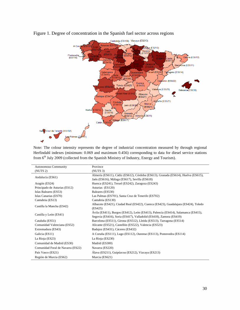
concentration. To illustrate our study framework, Figure 1 provides an outline of the
political sub-division by provinces and autonomous communities, as well as the market
concentration in each of the regions.
[Please insert Figure 1 here]
In order to perform the empirical analysis we have 728 daily data (from 1st October 2008 to
28th
September 2010) on the average retail fuel oil prices fixed by service stations in each
8
of the fifty provinces described above (excluding the autonomous cities of Ceuta and
Melilla). This dataset was provided by the Spanish Ministry of Industry, Tourism and
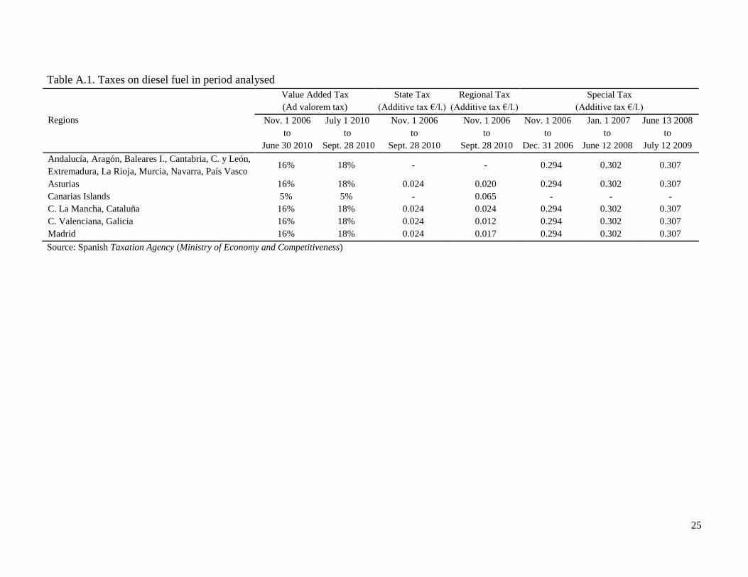
Trade.7 We have excluded all taxes from these prices. More specifically, the special tax on
hydrocarbons, the general tax established by the State, the taxes applied by each
autonomous community and value added tax (VAT) have all been removed in accordance
with information published by the Spanish Ministry of Economy’s Tax Office.8 We have
also considered the international spot prices (in fob terms) of the corresponding refined oil
product, which has been widely considered the most important direct cost for fuel retailers.
International oil prices, which are collected from the Energy Information Administration,
refer to the daily value of the refined oil product on the Amsterdam-Rotterdam-Antwerp
market. On weekends and holidays, where observations are missing as a consequence of
closure of the spot oil market, the wholesale prices from the day before will be applied.
Because international wholesale prices are collected in dollar terms (per litre), we convert
these prices into the local Spanish currency (Euro). For this purpose, we used the daily
Dollar/Euro exchange rate obtained from the Eurostat database.
2.3. Econometric specification
The fuel oil prices (measured in local terms for each province) in our sample differ from
theoretical fob prices described in Eq. (1) and Eq. (2). In fact, available retail prices include
transportation costs from different locations of oil refineries and local distribution costs,
which are unknown to us. With the aim of specifying an estimable empirical model, we
7 Sellers must report the set of retail prices at a sales point to the Ministry every Monday and also whenever
prices change (in accordance with the Ministerial Order ITC/2308/2007). In general, there are many service
stations that send information about changes in their selling prices several days per week.
8 Appendix A shows detailed information about each of the taxes applied on retail diesel fuel.
9
assume that these sorts of costs are time invariable, but still allowing for cross-sectional
heterogeneity. Then, differences between theoretical (fob) retail prices ( ) and local retail
prices can be captured by individual fixed effects ( ). In order to test the market
integration hypothesis we propose the following empirical model:
∑
∑
( )
where coefficients and will allow us to control for possible effects on retail prices of
seasonal changes in demand for month k and day q, respectively, with respect to a reference
time point (k = 1 and q = 1). The slopes can be interpreted as an empirical
approximation to the raw material cost pass-through for each of the R regions. Lastly, is
a random disturbance term, which is assumed to be iid.
We use available wholesale prices of refined fuel oil as a measure of raw material costs
( ).9 So, a comparative response of final prices to changes in refined fuel oil costs can
provide useful information about how far regions move away from a situation of market
integration. On the one hand, in cases where firms operate in a perfectly integrated market,
any common variation in refined fuel oil costs should be transmitted equally to final prices
in all regions. In terms of Eq. (3), this implies that (for overall i=1,..,R). That is,
for example, the particular extreme case of a perfectly competitive market where common
changes in marginal costs derived from refined fuel oil wholesale prices should be fully
transmitted to final retail prices ( . On the other hand, possible cases where the
9 As recommended for the measurement of oil raw material cost pass-through, we take prices for refined oil
instead of the spot price of crude oil (e.g. Borenstein et al., 1997). The reason for this is that our retail prices
should be treated as independent of the demand for other products derived from crude oil (due to joint
production in the industry).
10
common variations in costs of raw material were persistently transmitted to a different
degree across regions could only be explained by the presence of market power
and geographical segmentation.
3. Empirical results and discussion
3.1. Cost pass-through estimates
According to the stationary properties of the time series analysed in Annex B, we can be
sure that retail and wholesale prices are cointegrated and so Eq. (3) can be considered a
stable long-run equilibrium. Additionally, in accordance with the modified Wald statistic
proposed by Greene and Zhang (2003) and Wooldridge (2002), the presence of
heteroskedasticity and serial correlation is detected respectively. We also considered the
possibility of cross-sectional dependence among regions. Since the number of individuals is
smaller than the number of time observations, we chose to employ the LM-statistic
proposed by Breusch and Pagan (1980). From the statistical test, we can clearly reject the
null hypothesis of no spatial dependence (with a p-value virtually equal to zero). In view of
the results of the diagnostic test, we decided to estimate the fixed-effects model represented
in Eq. (3) by performing OLS with the standard errors of Driscoll and Kraay (1998). The
standard errors will thereby be corrected for heteroskedasticity and, furthermore, will be
robust to very general forms of temporal and spatial dependence.
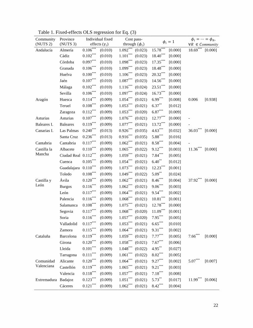
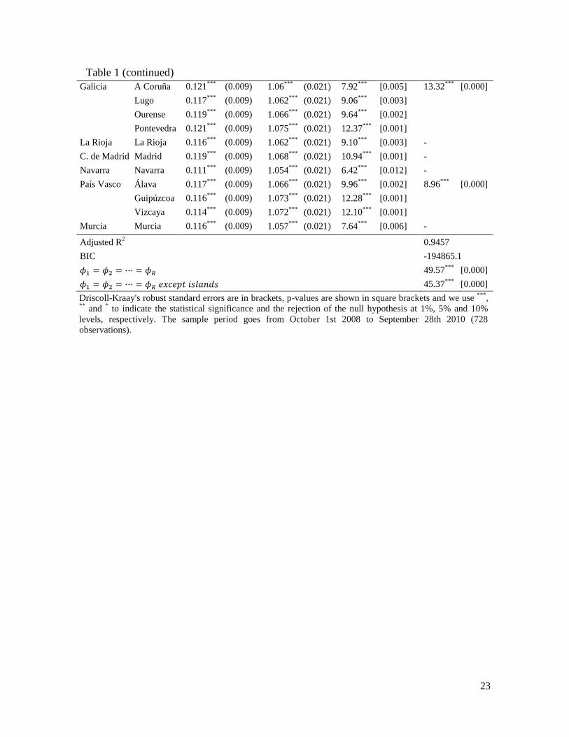
[Please insert Table 1 here]

11
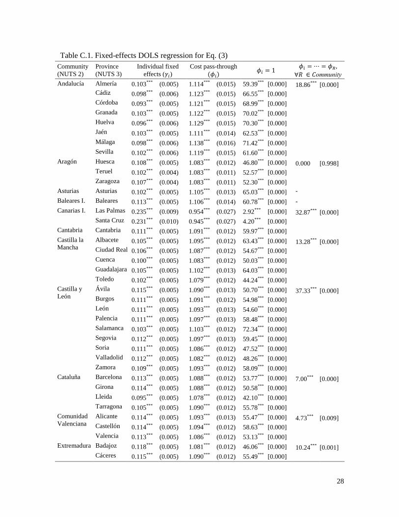
The individual fixed effects and the point estimates for raw material cost pass-through are
reported in Table 1.10
Estimates of individual fixed effects may reflect transportation costs
from different locations of oil refineries and local distribution costs. In this sense, this could
be consistent with the higher values obtained for provinces belonging to the Canarias
Islands. We are particularly interested in the estimates of raw material cost pass-through,
which are quite close to unity. However, in all cases, we can clearly reject the idea that
changes in raw material cost are fully transmitted to final prices. These empirical results are
not compatible with a situation of a fully integrated, perfectly competitive market
framework (i.e. ). Furthermore, we can also reject the null hypothesis related
with homogeneous cost pass-through among the fifty provinces ( ). This is also
true even after excluding the island territories from the sample (i.e. Baleares Islands and the
provinces that belong to Canarias Islands). Hence, the empirical outcomes suggest that the
Spanish regional markets are segmented even when we are dealing with the peninsular
territory.
Finally, with the aim of checking the robustness of the empirical results presented in Table
1, we have alternatively estimated the long-run equilibrium relationship from Eq. (3) by
using the dynamic OLS methodology for cointegrated panel data proposed by Kao and
Chiang (2000). As we can see in Annex C (Table C1), the results from the dynamic
empirical model are consistent with those discussed above.
10
A diagnostic test concerning the functional form has also been performed from our data. According to
Akaike Information Criterion (AIC), the model specification in levels is better than a double-log model
specification.

12
3.2. Cost pass-through differences
We formally explore the possibility of raw material cost pass-through being equal within
the same autonomous community (NUTS 2), but perhaps differing from one to another.
Therefore, we perform empirical tests which are shown in the last column of Table 1 (and
Table C1). Results indicate that, with the exception of Aragón, there is still a significant
degree of heterogeneity in the cost pass-through among provinces that belong to the same
autonomous community.
However, in spite of the heterogeneity, it seems that the magnitude of our point estimates
presented in Table 1 (and Table C1) could be linked to some extent to the division of
regions in autonomous communities. That is, in general, the degree of cost transmission for
provinces belonging to the same autonomous community seems more similar than in the
case of provinces that belong to different communities. This fact can be shown quite clearly
by a comparison of the provinces associated to the extreme values for estimated
coefficients. Thus, the two provinces belonging to the autonomous community Canarias
Islands correspond to the lowest estimated values. More specifically, we are referring to
Las Palmas and Santa Cruz de Tenerife. The opposite case is represented by the eight
provinces in the Community of Andalucía. That is, the highest estimated values are those
associated to the provinces of Málaga, Huelva, Cádiz, Granada, Córdoba, Sevilla, Almería
and Jaén.
We are therefore interested in formally exploring whether cross-sectional similarity in the
degree of estimated cost pass-through for a set of provinces can be explained well by a
latent factor associated to the autonomous community (e.g. the legal rules and discretionary
13
policy of each autonomous government). With this purpose in mind, let us further consider
a basic estimated dependent variable model (EDV) with the aim of analysing the
determinants of cost pass-through differences between provinces:
| | (4)
where the partner combinations of estimated regional coefficients of cost pass-through
and from Eq. (3) are regressed on a constant, a measure of proximity between provinces
(proximity) with the aim of controlling for typical spatial spillover effects, and a dummy
variable (community) that equals 1 if i and j belong to the same autonomous community
and 0 otherwise. Lastly, is a random disturbance term assumed to be iid.
We use alternative measures to capture the possible effect on cost pass-through similarity
derived from spatial proximity: boundary (as a dummy variable that takes a value of 1 if the
two regions share a common boundary and 0 otherwise), inverse of distance between the
capital cities of both regions and, lastly, inverse of squared distance between the capital
cities of both regions. The reason for considering the inverse distance between capital cities
as an approximation of spatial proximity among service stations is because the area around
these cities is where there are more stations in each province. Since the presence of an
estimated dependent variable can introduce heteroskedasticity into the regression
(Saxonhouse, 1976), we decided to apply OLS with White's consistent standard errors, as is
usual in these kinds of econometric specifications.

14
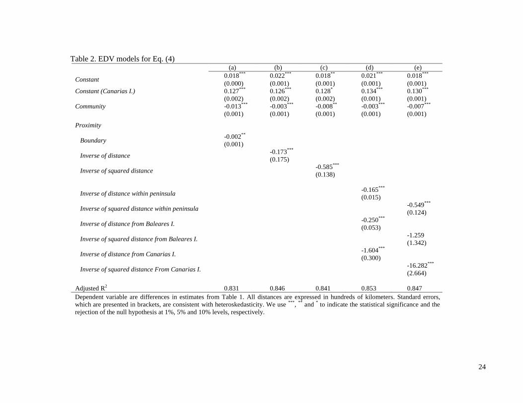
Empirical results for the spatial measures of geographical proximity discussed above are
shown in Table 2 (columns a, b, and c).11
As can be seen, the regression equations explain
more than 80% of the total variance of the differences in pass-through between provinces,
regardless of the alternative measures for spatial proximity between the provinces.
Estimated coefficients suggest that the presence of spillover effects among provinces is
quite significant. Therefore, after controlling for these spillover effects, we can know
whether belonging to the same autonomous community reduces the differences in cost
pass-through among provinces. Furthermore, regardless of the alternative specification
performed, the coefficients associated to the community variable always have a negative
sign and are highly significant. This indicates that the degree of cost transmission for those
provinces that share specific rules and a common political framework in oil fuel
distribution is clearly more similar.
[Please insert Table 2 here]
Finally, some additional considerations may be taken into account in the specification
model due the nature of the provinces included in our dataset. In this sense, because the
sample includes data for both peninsular and island territories, an appropriate empirical
strategy could be to split the coefficients. To be able to split coefficients we focus on
inverse distance because the goodness of fit of regressions when this control variable is
used is always greater than when the boundary variable is used. Then, on the one hand, we
will control for inverse distance between pairs of capital cities of provinces that belong to
the peninsula. On the other hand, we separately control for inverse distance when at least
11
We acknowledge possible unobserved effects linked with the Canarias Islands, mainly due to the region’s
idiosyncratic fuel taxes. Thus, we split the constant of the regression equation: one constant if the partner
regions or considered are Las Palmas or Santa Cruz de Tenerife and another for the rest of the cases.
15
one of the insular provinces is involved. Empirical results are provided in the last two
columns of Table 2 (columns d and e). The best goodness of fit is obtained for the most
general regression (column g). In any case, the estimated coefficients derived from all the
regressions performed are widely consistent with those discussed above and the
community-associated coefficient is always negative and highly significant.
4. Concluding remarks
This paper focuses on the comparison of the transmission of price variations of raw oil
material across regions. We found that the degree of cost pass-through to retail prices
differs significantly across the Spanish provinces, thereby suggesting a lack of market
integration at the regional level. In line with the existing evidence for the USA (i.e. Paul et
al., 2001; Slade, 1986), we found that more integration in retail oil markets is still possible.
These previous findings indicate that distance between the US regions explains the
presence of segmentation. However, since we have obtained cross-sectional estimates for
cost transmission, we can also ask ourselves whether there is a regional effect in market
segmentation derived from the existence of autonomous communities in Spain.
After controlling for the possible spillover effects across neighbouring regions, we explored
whether belonging to different autonomous community has some influence. We found that
there is more similarity in the raw material cost pass-through among provinces that belong
to the same autonomous community than in the rest of them. This effect according to
autonomous community could be attributed to discretional behaviour by the autonomous
regional governments, which is ultimately supported by the Spanish legislation framework.
That is, perhaps the difference in criteria across regional governments when they promote
16
and give administrative authorization to companies to operate in their territory plays an
important role in the existence of segmentation at the regional level. In sum, our results
suggest complete integration will be difficult without unification of the current legislation
and policies regarding the sector at the national level, as a step towards a larger single
European market for oil products. Obviously, the inherent behaviour of a highly
concentrated industry may also be behind the existence of the regional market segmentation
found in the study reported in this paper. To identify other factors of market behaviour that
become substantial drawbacks to integration in the oil retail industry, further work based on
firm-level data is required.
Acknowledgements
The authors wish to thank Massimo Filippini and the participants at the 12th
IAEE
European Conference in Venice. Any remaining errors are ours. Financial support from the
Spanish Ministry of Economy and Competitiveness (ECO2011-28155) and the Generalitat
Valenciana (VALI+D, ACIF/2010) are gratefully acknowledged.

17
Appendix A. Taxes
[Please insert Table A.1 here]
Appendix B. Time series properties
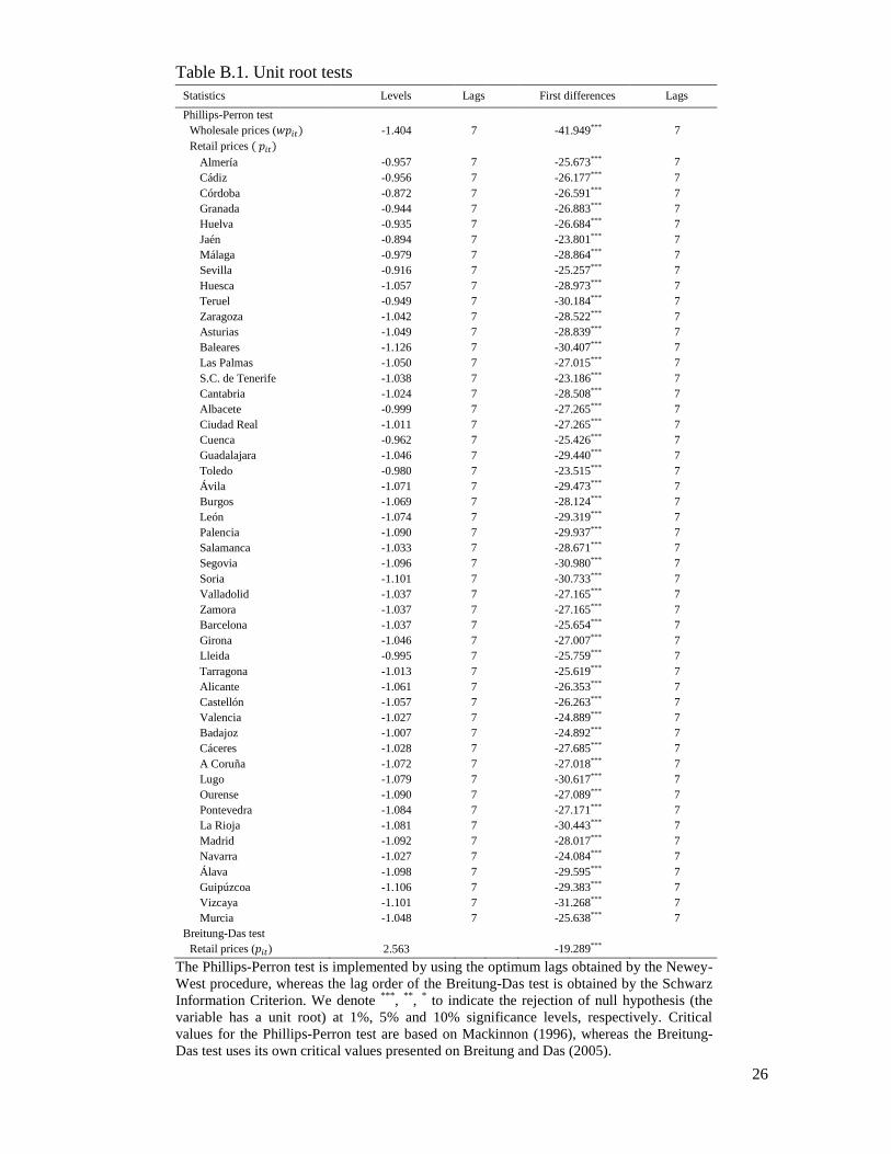
We use the unit root test proposed by Phillips-Perron (1988) on common wholesale prices
and retail prices for each separate region. However, the power of this last test can be low
when data combine both time-series and cross-sectional dimensions. Then, we additionally
employ the Breitung and Das (2005) unit root test on retail prices, since this statistic is
particularly suitable for panels with T ≥ N and the presence of cross-sectional
dependence.12
The corresponding results shown in Table B.1 indicate that both wholesale
and retail prices in levels are non-stationary, but after taking first differences we can reject
the null hypothesis of non-stationarity of the series (at the 0.01 level of significance). We
can therefore conclude that prices are integrated of order one, I(1).
[Please insert Table B.1 here]
To avoid a spurious regression by the potential presence of unit roots in variables from Eq.
(3), we must make sure that cointegration exists between retail and wholesale prices. If the
linear combination between dependent and independent variables is stationary I(0) while
each variable contains a unit root I(1), then Eq. (3) will represent a stable long-run
relationship. A methodology to test for cointegration under possible cross-sectional
12 In the panel unit root approach, we can distinguish a first group of tests based on the restrictive assumption
of cross-sectional independence (e.g. Maddala and Wu, 1999; Levin et al., 2002; Im et al., 2003). However,
Monte-Carlo simulations show that under cross-sectional dependence these panel tests may suffer from severe
size distortions. In fact, it is revealed that there is a tendency to over-reject the null hypothesis of unit root
(O’Connell, 1998; Breitung, 2002). Therefore, to address this problem, we use the robust OLS t-statistic
proposed by Breitung and Das (2005).

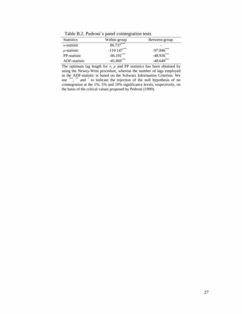
18
dependency is provided by Pedroni (1999, 2004). This author developed two types of tests
taking into account the residuals of the long-run equation. The first type is distributed as
being asymptotically standard-normal and is based on pooling the within-group residuals
for a long-run equation. The second type is also distributed as asymptotically standard-
normal, but is based on pooling the between-group residuals. Whereas the first type of
statistics is a panel version, the second statistics are based on averaging the corresponding
time series unit root test statistics. If all seven tests reject the null of non-cointegration
simultaneously, it is easy to draw a conclusion. Unfortunately, this is not always the case. If
the panel is large enough, so that size distortion is less of an issue, the panel υ-statistic tends
to have the best power relative to the other statistics and can be most useful when the
alternative is potentially very close to the null. Pedroni’s tests are presented in Table B.2.
All statistics can reject the null hypothesis of non-cointegration and, therefore, we can
verify that the linear combination between retail and refined prices moves jointly in the
long term.
[Please insert Table B.2 here]
Appendix C. Panel DOLS estimates of long-run cost pass-through from Eq. (3)
[Please insert Table C.1 here]
19
References
Bachmeier, L.J., Griffin, J.M. (2003). “New Evidence on Asymmetric Gasoline Price
Responses.” Review of Economics and Statistics 85(3): 772-776.
Bacon, R. (1991). “The Asymmetric Speed of Adjustment of UK Retail Gasoline Prices to
Cost Changes.” Energy Economics 13(3): 211-218.
Balaguer, J. (2011). Cross-border Integration in the European Electricity Market. “Evidence
from the pricing behavior of Norwegian and Swiss exporters.” Energy Policy 39(9): 4703-
4712.
Balaguer, J., Ripollés, J. (2012). “Testing for Price Response Asymmetries in the Spanish
Fuel Market. New Evidence from Daily Data.” Energy economics, forthcoming.
Borenstein, S., Cameron, A.C., Gilbert, R. (1997). “Do Gasoline Prices Respond
Asymmetrically to Crude Oil Price Changes?” Quarterly Journal of Economics 112(1):
305-339.
Breitung, J. (2002). “Nonparametric Tests for Unit Roots and Cointegration.” Journal of
Econometrics 108(2): 343-363.
Breitung, J., Das, S. (2005). “Panel Unit Root Tests Under Cross-sectional Dependence.”
Statistica Neerlandica 59(4): 414-433.
Breusch, T.S., Pagan, A.R. (1980). “The Lagrange Multiplier Test and its Applications to
Model Specification in Econometrics.” Review of Economic Studies 47(146): 239-254.
Dreher, A., Krieger, T. (2008). “Do Prices for Petroleum Products Converge in a Unified
Europe with Non-harmonized Tax Rates?” The Energy Journal 29(1): 61-88.
Dreher, A., Krieger, T. (2010). “Diesel Price Convergence and Mineral Oil Taxation in
Europe.” Applied Economics 42(15): 1955-1961.
Driscoll, J.C., Kraay, A.C. (1998). “Consistent Covariance Matrix Estimation with
Spatially Dependent Panel Data.” The Review of Economics and Statistics 80(4): 549-560.
20
Goldberg, P.K., Knetter, M.M. (1997). “Goods Prices and Exchange Rates: What Have we
Learned?” Journal of Economic Literature 5(3): 1243-1272.
Greene, W.H., Zhang, C. (2003). Econometric Analysis, Vol. 5. Prentice Hall, Upper
Saddle River, NJ.
Im, K.S., Pesaran, H.M., Shin, Y. (2003). “Testing for Unit Roots in Heterogeneous
Panels.” Journal of Econometrics 115(1): 53-74.
Joskow, P.L. (2008). “Lessons Learned from Electricity Market Liberalization.” The
Energy Journal 29(Special issue 2): 9-42.
Kao, C. and Chiang, M.H. (2000). “On the Estimation and Inference of a Cointegrated
Regression in Panel Data.” Advances in Econometrics 15: 179-222.
Levin, A., Lin, C.F. and Chu, C. (2002). “Unit Root Tests in Panel Data: Asymptotic and
Finite Sample Properties.” Journal of Econometrics 108(1): 1-24.
Maddala, G.S., Wu, S. (1999). “A Comparative Study of Unit Root Tests with Panel Data
and New Simple Test." Oxford Bulletin of Economics and Statistics 61(1): 631-652.
O’Connell, P.G.J. (1998). “The Overvaluation of Purchasing Power Parity.” Journal of
International Economics 44(1): 1-19.
Paul, R.J., Miljkovic, D., Ipe, V. (2001). “Market Integration in US Gasoline Markets.”
Applied Economics 33(10): 1335-1340.
Pedroni, P. (1999). “Critical Values for Cointegration Tests in Heterogeneous Panels with
Multiple Regressors.” Oxford Bulletin of Economics and Statistics 61(Special issue): 653-
670.
Pedroni, P. (2004). “Panel Cointegration: Asymptotic and Finite Sample Properties of
Pooled Time Series Tests with an Application to the PPP Hypothesis.” Econometric Theory
20(3): 597-625.
21
Phillips, P.C.B., Perron, P. (1988). “Testing for Unit Roots in Time Series Regression.”
Biometrika 75(2): 335-346.
Saxonhouse, G.R. (1976). “Estimated Parameters as Dependent Variables.” American
Economic Review 66(1): 178-83.
Slade, M.E. (1986). “Conjectures, Firms Characteristics, and Market Structure: An
Empirical Assessment.” International Journal of Industrial Organization 4(4): 347-370.
Smeers, Y. (1997). “Computable Equilibrium Models and the Restructuring of the
European Electricity and Gas Markets.” The Energy Journal 18(4): 1-31.
Vassilopoulos, P. (2010). Price Signals in “Energy-Only” Wholesale Electricity Markets:
An Empirical Analysis of the Price Signal in France.” The Energy Journal 31(3): 83-112.
Wooldridge, J.M. (2002). Econometric Analysis of Cross Section and Panel Data.
Cambridge, MA: MIT Press.
22
Table 1. Fixed-effects OLS regression for Eq. (3)
Community
(NUTS 2)
Province
(NUTS 3)
Individual fixed
effects ( )
Cost pass-
through
Andalucía Almería 0.106***
(0.010) 1.092***
(0.023) 15.78***
[0.000] 18.69***
[0.000]
Cádiz 0.102***
(0.010) 1.101***
(0.023) 18.40***
[0.000]
Córdoba 0.097***
(0.010) 1.098***
(0.023) 17.35***
[0.000]
Granada 0.106***
(0.010) 1.099***
(0.023) 18.48***
[0.000]
Huelva 0.100***
(0.010) 1.106***
(0.023) 20.32***
[0.000]
Jaén 0.107***
(0.010) 1.087***
(0.023) 14.56***
[0.000]
Málaga 0.102***
(0.010) 1.116***
(0.024) 23.51***
[0.000]
Sevilla 0.106***
(0.010) 1.097***
(0.024) 16.73***
[0.000]
Aragón Huesca 0.114***
(0.009) 1.054***
(0.021) 6.99***
[0.008] 0.006 [0.938]
Teruel 0.108***
(0.009) 1.053***
(0.021) 6.37**
[0.012]
Zaragoza 0.112***
(0.009) 1.053***
(0.020) 6.87***
[0.009]
Asturias Asturias 0.107***
(0.009) 1.076***
(0.021) 12.77***
[0.000] -
Baleares I. Baleares 0.119***
(0.009) 1.077***
(0.021) 13.72***
[0.000] -
Canarias I. Las Palmas 0.240***
(0.013) 0.926***
(0.035) 4.63***
[0.032] 36.03***
[0.000]
Santa Cruz 0.236***
(0.013) 0.916***
(0.035) 5.88***
[0.016]
Cantabria Cantabria 0.117***
(0.009) 1.062***
(0.021) 8.58***
[0.004] -
Castilla la
Mancha
Albacete 0.110***
(0.009) 1.065***
(0.022) 9.12***
[0.003] 11.36***
[0.000]
Ciudad Real 0.112***
(0.009) 1.059***
(0.021) 7.84***
[0.005]
Cuenca 0.105***
(0.009) 1.054***
(0.021) 6.40**
[0.012]
Guadalajara 0.110***
(0.009) 1.073***
(0.021) 12.23***
[0.001]
Toledo 0.108***
(0.009) 1.049***
(0.022) 5.09**
[0.024]
Castilla y
León
Ávila 0.120***
(0.009) 1.062***
(0.021) 8.46***
[0.004] 37.92***
[0.000]
Burgos 0.116***
(0.009) 1.062***
(0.021) 9.06***
[0.003]
León 0.117***
(0.009) 1.064***
(0.021) 9.54***
[0.002]
Palencia 0.116***
(0.009) 1.068***
(0.021) 10.81***
[0.001]
Salamanca 0.108***
(0.009) 1.075***
(0.021) 12.78***
[0.000]
Segovia 0.117***
(0.009) 1.068***
(0.020) 11.09***
[0.001]
Soria 0.116***
(0.009) 1.057***
(0.020) 7.95***
[0.005]
Valladolid 0.117***
(0.009) 1.053***
(0.021) 6.65***
[0.010]
Zamora 0.115***
(0.009) 1.064***
(0.021) 9.31***
[0.002]
Cataluña Barcelona 0.119***
(0.009) 1.059***
(0.021) 7.77***
[0.005] 7.66***
[0.000]
Girona 0.120***
(0.009) 1.058***
(0.021) 7.67***
[0.006]
Lleida 0.101***
(0.009) 1.048***
(0.022) 4.95**
[0.027]
Tarragona 0.111***
(0.009) 1.061***
(0.022) 8.02***
[0.005]
Comunidad
Valenciana
Alicante 0.120***
(0.009) 1.064***
(0.021) 9.27***
[0.002] 5.07***
[0.007]
Castellón 0.119***
(0.009) 1.065***
(0.021) 9.21***
[0.003]
Valencia 0.118***
(0.009) 1.057***
(0.021) 7.18***
[0.008]
Extremadura Badajoz 0.123***
(0.009) 1.051***
(0.021) 5.73**
[0.017] 11.99***
[0.006]
Cáceres 0.121***
(0.009) 1.062***
(0.021) 8.42***
[0.004]
23
Table 1 (continued)
Galicia A Coruña 0.121***
(0.009) 1.06***
(0.021) 7.92***
[0.005] 13.32***
[0.000]
Lugo 0.117***
(0.009) 1.062***
(0.021) 9.06***
[0.003]
Ourense 0.119***
(0.009) 1.066***
(0.021) 9.64***
[0.002]
Pontevedra 0.121***
(0.009) 1.075***
(0.021) 12.37***
[0.001]
La Rioja La Rioja 0.116***
(0.009) 1.062***
(0.021) 9.10***
[0.003] -
C. de Madrid Madrid 0.119***
(0.009) 1.068***
(0.021) 10.94***
[0.001] -
Navarra Navarra 0.111***
(0.009) 1.054***
(0.021) 6.42***
[0.012] -
País Vasco Álava 0.117***
(0.009) 1.066***
(0.021) 9.96***
[0.002] 8.96***
[0.000]
Guipúzcoa 0.116***
(0.009) 1.073***
(0.021) 12.28***
[0.001]
Vizcaya 0.114***
(0.009) 1.072***
(0.021) 12.10***
[0.001]
Murcia Murcia 0.116***
(0.009) 1.057***
(0.021) 7.64***
[0.006] -
Adjusted R2 0.9457
BIC -194865.1
49.57***
[0.000]
45.37***
[0.000]
Driscoll-Kraay's robust standard errors are in brackets, p-values are shown in square brackets and we use ***
, **
and * to indicate the statistical significance and the rejection of the null hypothesis at 1%, 5% and 10%
levels, respectively. The sample period goes from October 1st 2008 to September 28th 2010 (728
observations).
24
Table 2. EDV models for Eq. (4) (a) (b) (c) (d) (e)
Constant 0.018
*** 0.022
*** 0.018
** 0.021
*** 0.018
***
(0.000) (0.001) (0.001) (0.001) (0.001)
Constant (Canarias I.)
0.127***
0.126***
0.128* 0.134
*** 0.130
***
(0.002) (0.002) (0.002) (0.001) (0.001)
Community -0.013***
-0.003***
-0.008**
-0.003***
-0.007***
(0.001) (0.001) (0.001) (0.001) (0.001)
Proximity
Boundary -0.002
**
(0.001)
Inverse of distance -0.173
***
(0.175)
Inverse of squared distance -0.585
***
(0.138)
Inverse of distance within peninsula -0.165
***
(0.015)
Inverse of squared distance within peninsula -0.549
***
(0.124)
Inverse of distance from Baleares I. -0.250
***
(0.053)
Inverse of squared distance from Baleares I. -1.259
(1.342)
Inverse of distance from Canarias I. -1.604
***
(0.300)
Inverse of squared distance From Canarias I. -16.282
***
(2.664)
Adjusted R2 0.831 0.846 0.841 0.853 0.847
Dependent variable are differences in estimates from Table 1. All distances are expressed in hundreds of kilometers. Standard errors,
which are presented in brackets, are consistent with heteroskedasticity. We use ***
, **
and * to indicate the statistical significance and the
rejection of the null hypothesis at 1%, 5% and 10% levels, respectively.
25
Table A.1. Taxes on diesel fuel in period analysed
Regions
Value Added Tax
(Ad valorem tax)
State Tax
(Additive tax €/l.)
Regional Tax
(Additive tax €/l.)
Special Tax
(Additive tax €/l.)
Nov. 1 2006
to
June 30 2010
July 1 2010
to
Sept. 28 2010
Nov. 1 2006
to
Sept. 28 2010
Nov. 1 2006
to
Sept. 28 2010
Nov. 1 2006
to
Dec. 31 2006
Jan. 1 2007
to
June 12 2008
June 13 2008
to
July 12 2009
Andalucía, Aragón, Baleares I., Cantabria, C. y León,
Extremadura, La Rioja, Murcia, Navarra, País Vasco 16% 18% - - 0.294 0.302 0.307
Asturias 16% 18% 0.024 0.020 0.294 0.302 0.307
Canarias Islands 5% 5% - 0.065 - - -
C. La Mancha, Cataluña 16% 18% 0.024 0.024 0.294 0.302 0.307
C. Valenciana, Galicia 16% 18% 0.024 0.012 0.294 0.302 0.307
Madrid 16% 18% 0.024 0.017 0.294 0.302 0.307
Source: Spanish Taxation Agency (Ministry of Economy and Competitiveness)
26
Table B.1. Unit root tests
Statistics Levels Lags First differences Lags
Phillips-Perron test
Wholesale prices ( -1.404 7 -41.949*** 7
Retail prices
Almería -0.957 7 -25.673*** 7
Cádiz -0.956 7 -26.177*** 7
Córdoba -0.872 7 -26.591*** 7
Granada -0.944 7 -26.883*** 7
Huelva -0.935 7 -26.684*** 7
Jaén -0.894 7 -23.801*** 7
Málaga -0.979 7 -28.864*** 7
Sevilla -0.916 7 -25.257*** 7
Huesca -1.057 7 -28.973*** 7
Teruel -0.949 7 -30.184*** 7
Zaragoza -1.042 7 -28.522*** 7
Asturias -1.049 7 -28.839*** 7
Baleares -1.126 7 -30.407*** 7
Las Palmas -1.050 7 -27.015*** 7
S.C. de Tenerife -1.038 7 -23.186*** 7
Cantabria -1.024 7 -28.508*** 7
Albacete -0.999 7 -27.265*** 7
Ciudad Real -1.011 7 -27.265*** 7
Cuenca -0.962 7 -25.426*** 7
Guadalajara -1.046 7 -29.440*** 7
Toledo -0.980 7 -23.515*** 7
Ávila -1.071 7 -29.473*** 7
Burgos -1.069 7 -28.124*** 7
León -1.074 7 -29.319*** 7
Palencia -1.090 7 -29.937*** 7
Salamanca -1.033 7 -28.671*** 7
Segovia -1.096 7 -30.980*** 7
Soria -1.101 7 -30.733*** 7
Valladolid -1.037 7 -27.165*** 7
Zamora -1.037 7 -27.165*** 7
Barcelona -1.037 7 -25.654*** 7
Girona -1.046 7 -27.007*** 7
Lleida -0.995 7 -25.759*** 7
Tarragona -1.013 7 -25.619*** 7
Alicante -1.061 7 -26.353*** 7
Castellón -1.057 7 -26.263*** 7
Valencia -1.027 7 -24.889*** 7
Badajoz -1.007 7 -24.892*** 7
Cáceres -1.028 7 -27.685*** 7
A Coruña -1.072 7 -27.018*** 7
Lugo -1.079 7 -30.617*** 7
Ourense -1.090 7 -27.089*** 7
Pontevedra -1.084 7 -27.171*** 7
La Rioja -1.081 7 -30.443*** 7
Madrid -1.092 7 -28.017*** 7
Navarra -1.027 7 -24.084*** 7
Álava -1.098 7 -29.595*** 7
Guipúzcoa -1.106 7 -29.383*** 7
Vizcaya -1.101 7 -31.268*** 7
Murcia -1.048 7 -25.638*** 7
Breitung-Das test
Retail prices ( ) 2.563 -19.289***
The Phillips-Perron test is implemented by using the optimum lags obtained by the Newey-
West procedure, whereas the lag order of the Breitung-Das test is obtained by the Schwarz
Information Criterion. We denote ***
, **
, * to indicate the rejection of null hypothesis (the
variable has a unit root) at 1%, 5% and 10% significance levels, respectively. Critical
values for the Phillips-Perron test are based on Mackinnon (1996), whereas the Breitung-
Das test uses its own critical values presented on Breitung and Das (2005).
27
Table B.2. Pedroni’s panel cointegration tests
Statistics Within-group Between-group
υ-statistic 86.737***
-
ρ-statistic -110.147***
-97.846***
PP-statistic -46.191***
-48.936***
ADF-statistic -45.869***
-48.649***
The optimum lag length for υ, ρ and PP statistics has been obtained by
using the Newey-West procedure, whereas the number of lags employed
in the ADF-statistic is based on the Schwarz Information Criterion. We
use ***
, **
and * to indicate the rejection of the null hypothesis of no
cointegration at the 1%, 5% and 10% significance levels, respectively, on
the basis of the critical values proposed by Pedroni (1999).
28
Table C.1. Fixed-effects DOLS regression for Eq. (3)
Community
(NUTS 2)
Province
(NUTS 3)
Individual fixed
effects ( )
Cost pass-through
Andalucía Almería 0.103***
(0.005) 1.114***
(0.015) 59.39***
[0.000] 18.86***
[0.000]
Cádiz 0.098***
(0.006) 1.123***
(0.015) 66.55***
[0.000]
Córdoba 0.093***
(0.005) 1.121***
(0.015) 68.99***
[0.000]
Granada 0.103***
(0.005) 1.122***
(0.015) 70.02***
[0.000]
Huelva 0.096***
(0.006) 1.129***
(0.015) 70.30***
[0.000]
Jaén 0.103***
(0.005) 1.111***
(0.014) 62.53***
[0.000]
Málaga 0.098***
(0.006) 1.138***
(0.016) 71.42***
[0.000]
Sevilla 0.102***
(0.006) 1.119***
(0.015) 61.60***
[0.000]
Aragón Huesca 0.108***
(0.005) 1.083***
(0.012) 46.80***
[0.000] 0.000 [0.998]
Teruel 0.102***
(0.004) 1.083***
(0.011) 52.57***
[0.000]
Zaragoza 0.107***
(0.004) 1.083***
(0.011) 52.30***
[0.000]
Asturias Asturias 0.102***
(0.005) 1.105***
(0.013) 65.03***
[0.000] -
Baleares I. Baleares 0.113***
(0.005) 1.106***
(0.014) 60.78***
[0.000] -
Canarias I. Las Palmas 0.235***
(0.009) 0.954***
(0.027) 2.92***
[0.000] 32.87***
[0.000]
Santa Cruz 0.231***
(0.010) 0.945***
(0.027) 4.20***
[0.000]
Cantabria Cantabria 0.111***
(0.005) 1.091***
(0.012) 59.97***
[0.000]
Castilla la
Mancha
Albacete 0.105***
(0.005) 1.095***
(0.012) 63.43***
[0.000] 13.28***
[0.000]
Ciudad Real 0.106***
(0.005) 1.087***
(0.012) 54.67***
[0.000]
Cuenca 0.100***
(0.005) 1.083***
(0.012) 50.03***
[0.000]
Guadalajara 0.105***
(0.005) 1.102***
(0.013) 64.03***
[0.000]
Toledo 0.102***
(0.005) 1.079***
(0.012) 44.24***
[0.000]
Castilla y
León
Ávila 0.115***
(0.005) 1.090***
(0.013) 50.70***
[0.000] 37.33***
[0.000]
Burgos 0.111***
(0.005) 1.091***
(0.012) 54.98***
[0.000]
León 0.111***
(0.005) 1.093***
(0.013) 54.60***
[0.000]
Palencia 0.111***
(0.005) 1.097***
(0.013) 58.48***
[0.000]
Salamanca 0.103***
(0.005) 1.103***
(0.012) 72.34***
[0.000]
Segovia 0.112***
(0.005) 1.097***
(0.013) 59.45***
[0.000]
Soria 0.111***
(0.005) 1.086***
(0.012) 47.52***
[0.000]
Valladolid 0.112***
(0.005) 1.082***
(0.012) 48.26***
[0.000]
Zamora 0.109***
(0.005) 1.093***
(0.012) 58.09***
[0.000]
Cataluña Barcelona 0.113***
(0.005) 1.088***
(0.012) 53.77***
[0.000] 7.00***
[0.000]
Girona 0.114***
(0.005) 1.088***
(0.012) 50.58***
[0.000]
Lleida 0.095***
(0.005) 1.078***
(0.012) 42.10***
[0.000]
Tarragona 0.105***
(0.005) 1.090***
(0.012) 55.78***
[0.000]
Comunidad
Valenciana
Alicante 0.114***
(0.005) 1.093***
(0.013) 55.47***
[0.000] 4.73***
[0.009]
Castellón 0.114***
(0.005) 1.094***
(0.012) 58.63***
[0.000]
Valencia 0.113***
(0.005) 1.086***
(0.012) 53.13***
[0.000]
Extremadura Badajoz 0.118***
(0.005) 1.081***
(0.012) 46.06***
[0.000] 10.24***
[0.001]
Cáceres 0.115***
(0.005) 1.090***
(0.012) 55.49***
[0.000]

29
Table C.1 (continued)
Galicia A Coruña 0.115***
(0.005) 1.088***
(0.013) 48.33***
[0.000] 12.07***
[0.000]
Lugo 0.112***
(0.005) 1.091***
(0.012) 53.74***
[0.000]
Ourense 0.113***
(0.005) 1.095***
(0.013) 51.78***
[0.000]
Pontevedra 0.116***
(0.005) 1.104***
(0.014) 57.43***
[0.000]
La Rioja La Rioja 0.111***
(0.005) 1.091***
(0.012) 53.06***
[0.000] -
C. de Madrid Madrid 0.114***
(0.005) 1.098***
(0.013) 60.53***
[0.000] -
Navarra Navarra 0.105***
(0.005) 1.083***
(0.012) 46.27***
[0.000] -
País Vasco Álava 0.111***
(0.005) 1.096***
(0.013) 53.69***
[0.000] 8.26***
[0.000]
Guipúzcoa 0.111***
(0.005) 1.102***
(0.013) 63.39***
[0.000]
Vizcaya 0.109***
(0.005) 1.101***
(0.013) 62.60***
[0.000]
Murcia Murcia 0.111***
(0.005) 1.087***
(0.012) 53.94***
[0.000] -
Adjusted R2 0.999
BIC -235418
49.80***
[0.000]
47.30***
[0.000]
Driscoll-Kraay's robust standard errors are in brackets, p-values are shown in square brackets and we use ***
, **
and * to indicate the statistical significance and the rejection of the null hypothesis at the 1%, 5% and
10% levels, respectively. The panel DOLS has been estimated by using fifteen lags and leads of the first
difference of the explanatory variable chosen by the Schwarz information criterion (Schwarz, 1978). The
sample period goes from October 1st 2008 to September 28th 2010 (728 observations).
30
Figure 1. Degree of concentration in the Spanish fuel sector across regions
Note: The colour intensity represents the degree of industrial concentration measured by through regional
Herfindahl indexes (minimum: 0.069 and maximum 0.456) corresponding to data for diesel service stations
from 6th
July 2009 (collected from the Spanish Ministry of Industry, Energy and Tourism).
Autonomous Community Province
(NUTS 2) (NUTS 3)
Andalucía (ES61) Almería (ES611), Cádiz (ES612), Córdoba (ES613), Granada (ES614), Huelva (ES615),
Jaén (ES616), Málaga (ES617), Sevilla (ES618)
Aragón (ES24) Huesca (ES241), Teruel (ES242), Zaragoza (ES243)
Principado de Asturias (ES12) Asturias (ES120)
Islas Baleares (ES53) Baleares (ES530)
Islas Canarias (ES70) Las Palmas (ES701), Santa Cruz de Tenerife (ES702)
Cantabria (ES13) Cantabria (ES130)
Castilla la Mancha (ES42) Albacete (ES421), Ciudad Real (ES422), Cuenca (ES423), Guadalajara (ES424), Toledo
(ES425)
Castilla y León (ES41) Ávila (ES411), Burgos (ES412), León (ES413), Palencia (ES414), Salamanca (ES415),
Segovia (ES416), Soria (ES417), Valladolid (ES418), Zamora (ES419)
Cataluña (ES51) Barcelona (ES511), Girona (ES512), Lleida (ES513), Tarragona (ES514)
Comunidad Valenciana (ES52) Alicante (ES521), Castellón (ES522), Valencia (ES523)
Extremadura (ES43) Badajoz (ES431), Cáceres (ES432)
Galicia (ES11) A Coruña (ES111), Lugo (ES112), Ourense (ES113), Pontevedra (ES114)
La Rioja (ES23) La Rioja (ES230)
Comunidad de Madrid (ES30) Madrid (ES300)
Comunidad Foral de Navarra (ES22) Navarra (ES220)
País Vasco (ES21) Álava (ES211), Guipúzcoa (ES212), Vizcaya (ES213)
Región de Murcia (ES62) Murcia (ES621)