Testing the Asset Pricing Model of Exchange Rateswith Survey Forecasts

Anna Naszodi and Robert Lieli

May 21, 2014

Abstract

This paper proposes a new test for the asset pricing model of exchange rates.It examines whether forecasts produced by market analysts are more consistentwith a simple random walk view of the exchange rate or with a non-trivial rationalexpectations asset pricing model. The exploited difference between the models isthat the forecast is an exponential function of the forecast horizon in the assetpricing model, while it is constant in the random walk model. The asset pricingmodel is shown to have significantly better in-sample and out-of-sample fit on surveydata. As a second contribution, the paper also investigates whether some commonlyconsidered macroeconomic fundamental variables are linked to the exchange rate ina way consistent with the asset pricing model. By using historical data and surveyforecasts on both the exchange rate and potential economic fundamentals, we findthat GDP, budget deficit, as well as short and long-term interest rates, are importantdeterminants of the exchange rate. They explain between 32 and 45 percent of thevariance in excess currency returns over the one year horizon.

Keywords: asset pricing model of exchange rates, latent fundamentals, disconnectpuzzle, survey forecast.

JEL: F31, F36, G13.

1 Introduction

Although the asset pricing view has become a widely used building block in the exchangerate literature, it has been rejected by many empirical studies due to its rather poor

∗This research project has been started while Anna Naszodi has visited the European Central Bank,and the Sveriges Riksbank. The authors gratefully acknowledge comments and suggestions from PeterBenczur, Stefano Corradin, Paul De Grauwe, Casper G. de Vries, Hans Dewachter, Andras Fulop, Raf-faella Giacomini, Marianna Grimaldi, Laszlo Halpern, Zoltan Jakab, Gabor Kezdi, Julia Kiraly, TamasKollanyi, Istvan Konya, Miklos Koren, Manfred Kremer, Tamas Papp, Genaro Sucarrat, Lars Svensson,Akos Valentinyi, Peter Westaway, and from the participants of presentations at the Central EuropeanUniversity, the European Central Bank, the Magyar Nemzeti Bank, and the Sveriges Riksbank. Specialthanks to Francesca Fabbri for her excellent research assistance at the European Central Bank.†The views expressed in this paper are those of the authors and do not necessarily reflect the official

view of the European Central Bank, the Magyar Nemzeti Bank (National Bank of Hungary), and theSveriges Riksbank (National Bank of Sweden).

1

out-of-sample forecasting performance (see Meese and Rogoff (1983)). Notably, it cannotsignificantly and systematically outperform even the atheoretical random walk modelin forecasting the major exchange rates. Engel and West (2005) question the standardcriterion based on out-of-sample forecasting for judging exchange rate models. Theyargue that under certain conditions the standard rational expectations asset pricing modelimplies that the exchange rate follows a near random walk process. Therefore, evidencethat these models do not beat the random walk in forecasting cannot be taken as evidenceagainst the models. It seems essential to look for other means of evaluating exchange ratemodels.

The main contribution of this paper is that it proposes a new test for the asset pricingmodel by exploiting its implications for how market participants form their expectationsabout future spot exchange rates. These expectations, on the other hand, are identifiedfrom survey forecasts; specifically, we assume that the observed consensus exchange rateforecasts are noisy versions of the prevailing market expectations. The test exploits afunctional form disparity between forecasts from the asset pricing model and its nestedalternative, the random walk model. The general asset pricing model implies that thelog exchange rate forecast is an exponential function of the forecast horizon, while in therandom walk model, the term-structure of forecasts is constant. This difference has notbeen investigated before in the context of testing the asset pricing model for exchangerates. We present evidence on the in-sample and out-of-sample fit of the models, andfind that the results clearly favor the asset pricing model. The interpretation is that theexchange rate model professional forecasters seem to have in mind is closer to a generalasset pricing model than to the random walk. If we further assume that forecasters as agroup would not, in the long run, use a misspecified model, then a stronger interpretationof the results is that the asset pricing model can be a reasonable approximation of theunderlying data generating process.

One potential reason for the rejection of the asset pricing model by the previous empir-ical literature is the misspecification of the structural macroeconomic models that definethe exchange rate fundamentals.1 Indeed, there is no consensus among economists overwhat the relevant macro fundamentals are. For instance, Engel and West (2005) presentwidely-used structural exchange rate models with reduced form representations that fitthe asset pricing framework, but with different implications about what the fundamentalsshould be. A related point is that the fundamental process might contain, or might evenbe dominated by, “some other variable[s] that models have not captured or that [are]unobserved”. ((Engel and West, 2005), p. 499). For example, the risk premium is oftenassumed to be a fundamental variable, but is generally unobservable.

Therefore, in testing the asset pricing model against the random walk, we take a lesstheoretical approach and treat the fundamental process as an unobserved latent variable.We show that one can use the Kalman filter to estimate this latent process from the timeseries of the spot exchange rate and the survey forecasts for various forecast horizons.Filtering the fundamental allows us to bypass the problem of committing to a specificstructural model and a specific definition of the fundamental.2 The key idea is that

1Besides the problem of misspecification, Meese and Rogoff (1983) also name simultaneous equationbias, sampling errors, and parameter instability as potential reasons for the disappointing forecastingperformance of linear macro models.

2The filtering approach has been applied by a number of previous papers in the literature. See forinstance, Gardeazabal et al. (1997), Burda and Gerlach (1993) and De Grauwe et al. (1999). This paper

2

market expectations about future spot rates are based on the relevant set of fundamentals(whatever they might be), and, again, that survey forecasts essentially capture marketexpectations. Thus, while our results are not contingent on a particular definition of thefundamental, they do rely on the aforementioned interpretation of survey forecasts.

Nevertheless, this atheoretical, and somewhat intrinsic, view of the fundamental canalso be construed as a weakness. The problem, in particular, is that the filtered funda-mental process is hard to interpret. This motivates the second part of the paper, where weinvestigate whether some commonly considered economic fundamentals are linked to theexchange rate in a way consistent with the asset pricing model. Specifically, the questionis whether the difference between the exchange rate forecast and the spot rate is purelydue to some unobservable factors, like market sentiment and risk premia, or it can partlybe explained by any of the traditionally considered economic fundamentals.

On the usually available rather short samples, it is difficult to find a strong, statis-tically significant and stable link between the major exchange rates and those economicindicators that are suggested by international macroeconomic theory to determine theseexchange rates. (Obstfeld and Rogoff (2000) called the missing empirical link betweenexchange rates and macroeconomic fundamentals the disconnect puzzle.) In this paper,we circumvent the short sample problem by using survey forecasts on both the exchangerate and its macro fundamentals in addition to the time series of the target variables ofthe forecasts. The idea is that the estimated empirical link between the forecasted ex-change rate and the forecasted fundamentals can be exploited to identify the relationshipbetween the exchange rate and the fundamentals. Once again, the identification relies onthe assumption that market expectations are formed on the basis of the “right” set macrofundamentals with the “right” set of weights, and the consensus forecasts are informativeabout market expectations. In addition to enriching the commonly used data by surveyforecasts, our identification strategy is also facilitated by running panel regressions insteadof estimating a model for each exchange rate separately.

We find that GDP, budget deficit, oil price together with the short and long interestrates are significant determinants of the seven major exchange rates investigated in thispaper. They explain a substantial part, between 32 and 45 percent of the variance inexcess currency returns over the one year horizon.

The rest of the paper is structured as follows. Section 2 introduces the asset pricingexchange rate model and describes the estimation strategy in more detail. Section 3presents the data and the empirical results. Finally, Section 4 concludes.

2 The Asset Pricing Exchange Rate Model

In the conventional class of asset-pricing models the exchange rate is the discounted sumof current and expected future fundamentals.3

st = (1− b)∞∑j=0

bjEt(xt+j) with 0 < b < 1 , (1)

distinguishes itself by using survey forecasts to back out the time series of the fundamental.3The asset pricing model of exchange rates has different names in the literature. It is called the “asset

market view model”by Frenkel and Mussa (1980), the “canonical model”by Krugman (1992) and byGardeazabal et al. (1997) and the “rational expectations present-value model”by Engel and West (2005).

3

where st denotes the log exchange rate at time t, while xt+j is the fundamental at timet + j. It is important to emphasize that xt+j captures not only the usually consideredobservable macroeconomic variables, but also the unobservable drivers of the exchangerate. Et(.) is the expectation operator, where the expectation is conditional on all theinformation available at time t. Finally, b is the discount factor.

Macroeconomic models that rationalize the asset pricing exchange rate model offerdifferent interpretations of parameter b. For instance, Engel and West (2005) reviewsome standard models, where b

1−b is either the semi-elasticity of money demand withrespect to the interest rate, or 1 − b is the relative weight of the exchange rate in theTaylor rule. As the empirical identification of the discount factor b is problematic for anumber of reasons discussed at a later point in this paper, we calibrate b by relying onthe parameter estimates of some structural models in previous empirical studies.

These structural models provide different definitions for the fundamental xt as well.As we do not use the definition of any of these models, our results are general to a broadclass of structural models. Part of the cost of this generality is that we have to make anassumption about the dynamics of the fundamental process. The assumed process of xtis AR(2); specifically,

xt = α + ϕ1xt−1 + ϕ2xt−2 + εx,t , where εx,t ∼ i.i.d.N(0, σ2x) . (2)

When the sum of the autoregressive parameters ϕ1 and ϕ2 is 1, the fundamental processhas a unit root. The special case of α = 0, ϕ1 = 1 and ϕ2 = 0 corresponds to therandom walk. In this case Et(xt+j) = xt, and equation (1) reduces to st = xt, i.e., the logexchange rate trivially follows a random walk regardless of b. Furthermore, past changesin the fundamentals can neither explain nor predict future changes in the log exchangerate. Regarding the general case, when α 6= 0 or ϕ1 6= 1 or ϕ2 6= 0, near random walkbehavior of the exchange rate is still possible. As it is pointed out by Engel and West(2005), one cannot find significant correlation between exchange rate returns and pastchanges in the fundamentals given that the fundamental process is highly persistent andthe discount factor b is ”sufficiently large”. Therefore, the random walk model is nestedpractically by the present-value asset pricing model under more than one set of parameterrestrictions.

To facilitate the identification of the latent fundamental xt from survey forecasts,it is helpful to express the expected future exchange rate as a function of present andpast fundamentals. As we show in the Appendix, Et(st+k), k ≥ 0, is given by the firstcomponent of the vector

(1− b)F k(I − bF )−1ξt , where ξt =

xtxt−1

1

and F =

φ1 φ2 α1 0 00 0 1

. (3)

In the special case of zero forecast horizon, k = 0, the expected exchange rate Et(st+k)is identical to the spot exchange rate st. The restriction k = 0 reduces equation (3) to

st =1− b

1− bϕ1 − b2ϕ2

xt +(1− b)bϕ2

1− bϕ1 − b2ϕ2

xt−1 +bα

1− bϕ1 − b2ϕ2

. (4)

Equation (4) shows how the spot exchange rate depends on the contemporaneous andprevious period value of the fundamental.

4

For k > 0, the forecast horizon appears in the expression for Et(st+k) as an exponent.This characteristic distinguishes the general asset pricing model from the random walkmodel, where forecasts are the same for all forecast horizons. Accordingly, if forecasts,on average, are equal to the theoretical expected value of the target variable, then the“typical” forecast from the asset pricing model must be an exponential function of theforecast horizon. More precisely, we assume that

zt,t+k = Et(st+k) + εt,k , (5)

where zt,t+k is the survey forecast at time t with forecast horizon k > 0. The error termεt,k has a Gaussian distribution, with zero expected value and constant variance denotedby σ2

z,k. The errors εt1,k1 and εt2,k2 for any time t1 and t2 (t1 6= t2) are assumed to beindependent, while errors of the forecasts formed at the same time t but with differentforecast horizons k1, k2 are allowed to be correlated. The correlation between εt,k1 andεt,k2 is denoted by ρz,k1,k2 .

Equations (2), (4) and (5) together with (3) form a state-space system, where (2) isa transition equation specifying the dynamics of the underlying state variable xt, andequations (4) and (5) are observation equations specifying the observed variables as anaffine function of xt, xt−1, and an error (after substituting in for Et(st+k) from equation(3)). The coefficients in this system, along with the process xt, is readily estimable bythe Kalman filter.

3 Empirical Analysis

This section tests some empirical implications of the present-value asset pricing model.Section 3.1 describes the data used in the analysis. Section 3.2 investigates whetherthe way market analysts generate their exchange rate expectations is closer to the oneimplied by the asset pricing model or to that implied by the random walk model. Section3.3 investigates which economic fundamentals drive and thought to drive the exchangerate.

3.1 Description of the Data

This section describes the data used in the empirical part of the paper. First, it introducesthe survey forecasts on exchange rates. These data are used both for testing the assetpricing model and also for identifying the relevant macro fundamentals in the secondempirical exercise. Second, it describes those macro data and their forecasts that areused only in the second exercise.

The survey data on exchange rate forecasts are from the Consensus Economics. Con-sensus Economics surveys the opinion of the market analysts every month. The surveyrespondents report their expected 3 months (0.25Y), 1 year (1Y), and 2 years (2Y) aheadend-of-month exchange rates.4 5 The survey data used in this paper is the mean of theindividual forecasts, therefore it mirrors the consensus view of the professional forecasters.

4The reported forecasts are not the expected log exchange rates, but the expected exchange rates inlevel. we proxy the expected log exchange rates by the log of the reported expected exchange rates in allcalculations and estimations.

5The forecast horizons usually differ from 3 months, 1 year, and 2 years by a few days, because thesurveys do not take place exactly at the end of each month, while the forecasts refer to the end-of-

5

The sample spans between January 1999 and September 2008. Therefore, the size ofthe time series dimension of the sample is 117. The size of the cross-sectional dimensionof the data is seven as the surveys cover the following seven major exchange rates: theCanadian dollar (CAD), euro (EUR), the United Kingdom pound (GBP), the Japaneseyen (JPY) against the US dollar (USD), and the Swiss franc (CHF), Norwegian krone(NOK), Swedish krona (SEK) against the euro.

For the second empirical exercise presented in this paper, we use the time series ofsome macroeconomic data together with their forecasts. The time series of the macrovariables and their forecasts are collected for the following 8 countries: Canada, Ger-many (representing the Eurozone), the United Kingdom (UK), Japan, the United States(US), Switzerland, Norway and Sweden. The sample of the economic variables (both thehistorical data and the survey forecasts) spans between January 1999 and January 2009.

Out of the forecasted variables in the Consensus Economics survey the natural can-didates of exchange rate fundamentals are the growth rate of the real gross domesticproduct (GDP, percent change per annum), government budget balance (in level in localcurrency),6 current account (CA, in level in local currency), consumer price index (CPI,percent change per annum), 3-month interest rates (in percent), 10-year government bondyields (in percent) and oil price (WTI price in USD per barrel).

As the exchange rate fundamentals are defined by the domestic and foreign countrydifferences of the economic indicators, and the original budget forecast and CA forecast arepublished in different currencies for different countries, they need to be transformed. Wetransform them into budget per GDP forecast and CA per GDP forecast by dividing theiroriginal forecasts by the forecasted GDP (also in level and in local currency). Thereby,the transformed data are already measured in the same quantity in the domestic andforeign countries.

Although the considered economic indicators and the survey forecasts are availableeven on monthly frequency, we work with data on annual frequency. The motivation forthat is two-fold. First, the annual series of economic indicators are more reliable as theyare not exposed to seasonality and less exposed to data revisions. Second, typically theforecast horizon in the surveys shrinks over the course of the year, because it is the end-of-year value of most of the economic indicators that is predicted. The exceptions are theinterest rate forecasts and the oil price forecasts, where the forecast horizon is 1 year nomatter in which month the forecast is produced.

The source of the survey forecasts on the macro variables is the same as that of theexchange rate forecasts, it is the Consensus Economics. The historical time series of theforecasted variables are from the following sources. The short-term and long-term interestrates are from Bloomberg, while the oil price is from Thomson Reuters Datastream. Theseries of the rest of the variables are from the OECD’s Main Economic Indicators database.

month exchange rates. For instance, the survey can be on the 15th of December of a given year and theparticipants of that survey are asked to forecast the end-of-March, end-of-December exchange rates ofthe coming year and the end-of-December exchange rate of the year after. Unfortunately, the discretetime model in this paper cannot account for such an irregularity of the forecast horizons.

6Forecast on government budget is published by the Consensus Economics only for Japan, Germany,Canada, the US and the UK out of the eight countries in our sample.

6

3.2 Testing the Asset Pricing Exchange Rate Model Based onits In-Sample Fit and Out-of-Sample Fit on Survey Fore-casts

One way of testing the competing models is to compare their in-sample and out-of-samplefit on survey forecasts. This section explains how the competing models are estimated forthese tests, what the test statistics are, and interprets the results.

When comparing the in-sample fit of the models the model parameters are estimatedfrom survey forecasts with all the three different forecast horizons (3 months, 1 year and2 years), and the exchange rate on the survey dates. After estimating the models by theKalman filter, we compare their filtering likelihoods by the likelihood ratio test. Underthe null hypothesis the random walk model and the asset pricing model fit the dataequally well. Given that the random walk model is nested by the asset pricing model, thelikelihood ratio test provides a theoretically valid comparison of the models.

In addition to comparing the in-sample performances of the models, we also checkwhich of the two models has better out-of-sample fit on the survey forecasts. For thisexercise the asset pricing model is estimated again by the Kalman filter. However, thistime only the survey forecasts with the two longer forecast horizons (1 year and 2 years),and the exchange rate on the survey date are used as observed variables, but not thesurvey forecasts with the 3-month horizon. The time series of the 3-month forecast issaved to measure the out-of-sample fit. We choose the forecast with the shortest forecasthorizon for the out-of-sample test, because distinguishing empirically between the randomwalk model and the asset pricing model is more difficult on the short horizon.

After estimating the asset pricing model, we investigate how close its fitted 3-monthforecast is to the 3-month survey forecast. In case of the random walk model, we do notneed to estimate the model in order to obtain its 3-month fitted forecast as it is identicalwith the spot rate. Accordingly, the models are judged by comparing the distance betweenthe fitted 3-month forecast of the asset pricing model and the 3-month survey forecast onthe one hand with the distance between the spot rate and the 3-month survey forecast onthe other hand.

The logic of the proposed out-of-sample test can be illustrated by a magician’s trick.The magician asks someone from the audience to tell her 1-year and 2-year exchange rateforecast. The person is asked to make a 3-month forecast as well, but instead of telling itto the magician, she should write it down on a piece of paper and hide it in an envelope.If the magician can find out the secret 3-month forecast, then he is likely to know howthe forecasts were generated. Moreover, if the forecaster is rational, the model she hasin mind is identical to the data generating process of the exchange rate. Therefore, asuccessful magician knows not only what the forecaster thinks, but also how the exchangerate is determined.

As we have already indicated in Section 2, we use the Kalman filter to estimate theunobserved fundamental process in the state space system given by equations (2), (4)and (5).7 This involves maximizing the filtering likelihood, which is undertaken by thesimulated annealing algorithm (see, e.g., Goffe et al. (1994)). When investigating thein-sample fit of the models, we use four observation equations, one for the spot rate and

7The Kalman filter toolbox for Matlab written by Kevin Murphy is used. See http://www.ai.mit.edu/murphyk/Software/kalman.html for details.

7

three for forecasts with horizons 3 months, 1 year and 2 years. When investigating theout-of-sample fit of the models, we use three observation equations, one for the spot rateand two for forecasts with horizons 1 year and 2 years.

All model parameters with the exception of the discount factor b are estimated. So,the following 10 parameters are estimated in the most general model specification, whenthere is no parameter restriction imposed and all the survey forecasts with three differentforecast horizons are used to filter out the fundamentals: ϕ1, ϕ2, α, σ2

x, σ2z,k=0.25Y , σ2

z,k=1Y ,σ2z,k=2Y , ρz,k1=0.25Y,k2=1Y ,ρz,k1=0.25Y,k2=2Y and ρz,k1=1Y,k2=2Y . As opposed to these param-

eters, setting the discount factor needs special care. Lieli and Naszodi (2013) write thefollowing on the problem of identifying the discount factor: ”if the fundamental process isa random walk, then the exchange rate will be a random walk as well regardless of whatthe value of the discount factor is. To put it somewhat differently, the discount factor isidentified solely by the dynamics in the first difference of the fundamental process; if thefirst difference is white noise (more exactly, martingale difference), then the model hassimply no implications about the discount rate.” Furthermore, even if the fundamentalprocess is not an exact random walk, just a near random walk, its estimation is stillproblematic on finite samples of usual length. For the above reason, the discount factorb is calibrated. Its calibrated value is chosen to be consistent with the previous empiricalliterature. Engel and West (2005, page 497) note that the implied range for the quarterlydiscount factor is of 0.97-0.98 based on the works of Bilson (1978), Frankel (1979), Stockand Watson (1993, 802, table 2, panel I). Therefore, the annual discount factor should bein the range of 0.885 - 0.922 , while the monthly discount factor should be in the rangeof 0.990 - 0.993. Accordingly, the annual discount factor is set to 0.9, while the monthlydiscount factor is set to 0.9913 in this paper.

3.2.1 Results of the Test and their Interpretations

Table 1 presents the parameter estimates of the asset pricing model obtained by usingall three survey forecasts. As the sum of the estimated autoregressive parameters is closeto unity for all investigated exchange rates, the fundamentals follow a highly persistentprocess. This finding is consistent with the first condition of Engel and West (2005)that implies the approximately random walk behavior of the exchange rate together withthe high discount factor condition. Table 2 presents the parameter estimates obtainedalso from all three survey forecasts, but this time the estimated model is the random walkmodel. Accordingly, the parameters α, ϕ1 and ϕ2 are restricted to 0, 1 and 0, respectively.

When comparing the likelihoods of the two models, we find the following. First, thelog likelihood of the broader model, i.e., that of the asset pricing model is higher thanthat of the nested random walk model for all seven currency pairs. See the last rows inTables 1 and 2. Second, the differences between the log likelihoods are sufficiently large toreject the null hypothesis of equal in-sample performance of the models at any meaningfulsignificance level. This is inferred from the likelihood ratio test statistics that follows achi-square distribution with three degrees of freedom given that the random walk modelis obtained from the asset pricing model by imposing three parameter restrictions.

Not surprisingly, the relative goodness of out-of-sample fit of the models also confirmthat the asset pricing model out-performs the random walk model. For this comparisonof the models, we re-estimate the asset pricing model on a restricted sample that does notcover the 3-month survey forecasts. Once the asset pricing model is estimated, we can

8

easily obtain its fitted 3-month exchange rate forecast zAPt,t+0.25Y by substituting the pointestimates of the parameters and the filtered fundamental into equation (3). Obtainingthe fitted 3-month exchange rate forecast that is consistent with the random walk modelzRWt,t+0.25Y is even simpler as being equal to st. Than, we compare the models by using astandard measure on how well they fit the survey data on the expected 3-month aheadexchange rate zt,t+0.25Y .

The goodness of fit is measured by the root mean square error (RMSE).8 Accordingly,the tested hypothesis is that the squared errors of the asset pricing model are equal tothat of the random walk model in expected term.

H0 : E[(zt,t+0.25Y − zRWt,t+0.25Y )2 − (zt,t+0.25Y − zAPt,t+0.25Y )2

]= 0 . (6)

The alternative hypothesis is that the asset pricing model has better out-of-sample fit:

H1 : E[(zt,t+0.25Y − zRWt,t+0.25Y )2 − (zt,t+0.25Y − zAPt,t+0.25Y )2

]> 0 . (7)

The formal test of the null is missing from this version of the paper. It is an ongoingwork to select the adequate test-statistics.

Table 3 shows that the asset pricing model has better out-of-sample fit for all sevencurrency pairs. It is worth to remark that the asset pricing model out-performs the randomwalk model not simply because of being broader. A model that is complex enough can fitthe data in-sample even perfectly as an extreme example of overfitting. However, the samemodel usually performs poorly out-of-sample. The intuitive explanation for this findingis that a sufficiently broad model is flexible enough to learn sample specific regularitiesand consider them falsely as part of the underlying relationship. Since the goodness of fitis measured out-of-sample in this second test, the good performance of the asset pricingmodel cannot be attributed to the model complexity and to the potential problem ofoverfitting.

The main finding of this section can be summarized as follows. It is proved that theasset pricing model fits the survey forecasts better than the random walk model does bothin-sample and out-of-sample. The intuitive explanation for this finding is that the term-structure of survey forecasts is closer to the exponential curve than to a constant. As itis shown in the theoretical part of this paper in section 2 the exponential term-structureis consistent with the non-trivial asset pricing model, while the constant term-structureis consistent with the random walk model. The exponential relationship between theforecast horizon and the forecast comes from the present-value relationship between thespot exchange rate and future fundamentals, where the discount factor is raised to ahigher power for fundamentals more distant in time. So, the finding that the asset pricingmodel fits the survey forecasts well, provides empirical support to the functional form ofthe asset pricing model of (1).

By analyzing survey forecasts, Frankel and Froot (1987) also reject the static expecta-tion hypothesis. It means that they can also confute that the process of the exchange rateis thought to be random walk by the survey participants. So, the empirical finding of thispaper is in line with the previous literature, while its interpretation is new. This paperinterprets the results in the context of testing the asset pricing model, while Frankel andFroot (1987) test a number of hypotheses on how the survey forecasts are produced.

8By using the mean absolute error as an alternative to the root mean square error, we obtain quali-tatively the same results.

9

3.3 Linking Exchange Rate and Economic Fundamentals

Unfortunately, the test proposed in this paper does not reveal what specific economicvariables are important determinants of the exchange rate given that the fundamentalis treated as unobservable. Theoretically, it is possible that the filtered fundamentalcaptures mainly some unobservable exchange rate fundamentals, like market sentimentand risk premia, and it fails to capture the traditionally considered observable economicfundamentals. Due to this possibility, this section complements the test by investigatingthe main economic drivers of exchange rate.

A straightforward approach for identifying the important economic determinants ofexchange rate would be to regress the filtered fundamental on various economic indicators.This method is clearly a 2-stage method, where the series of fundamental is filtered in thefirst stage, while the coefficients of its economic components are estimated in the secondstage. The shortcoming of 2-stage methods in general is that it is difficult to take intoaccount in the second stage that the series obtained from the first stage is not directlyobserved, but are themselves estimates and so contain sampling variation. Due to thisissue, we do not use the series of the filtered fundamental in this section. And we identifythe economic determinants of exchange rate directly from some observed series.

The analysis in this section centers on the following empirical questions. First, whatare the economic fundamentals that drive the exchange rate. Second, what are the eco-nomic fundamentals that are thought to drive the exchange rate by the representativeforecaster. The important economic determinants of the exchange rate are identified byassuming that the answers to the above two questions are the same.

In this section, we define the fundamental xt as the index of some economic indicators.

xt =J∑j=1

αjyt,j , (8)

where yt,j denotes the jth macroeconomic indicator at time t (also called as the economicfundamentals of exchange rate) and αj is its weight.

By rearranging the asset pricing equation (1) in two ways, we can make it explicit,how the exchange rate is determined by its present and future fundamentals and by theexpected future exchange rate (which is also determined by the future fundamentals). Weobtain

st = bEt(st+1) + (1− b)xt , (9)

and

st = b2Et(st+2) + (1− b) [xt + bEt(xt+1)] . (10)

Equation (9) describes the link between the spot exchange rate st and the present funda-mental xt, while equation (10) captures how the expected future exchange rate Et(st+2)is related to the expected future fundamental Et(xt+1). As we are primarily interested inthe first link, the latter link is used only for identifying the former that is in the center ofour interested.

By substituting (8) into (9) and (10), and by proxying the expected exchange rates(Et(st+1) and Et(st+2)) and the expected fundamental components (Et(yt+1,j)) by theirsurvey counterparts, we obtain the system of equations of (11) and (12) that is ready to

10

be estimated.

st = bzt,t+1 + (1− b)J∑j=1

αjyt,j + η1 , where η1 ∼ i.i.d.N(0, σ2η1

) . (11)

st = b2zt,t+2 + (1− b)J∑j=1

αj [yt,j + bvt,t+1,j] + η2 , where η2 ∼ i.i.d.N(0, σ2η2

) . (12)

where vt,t+1,j denotes the survey forecast on the 1 period (1 year) ahead jth component ofthe fundamentals, while zt,t+k is the survey forecast on the k period ahead log exchangerate like before.

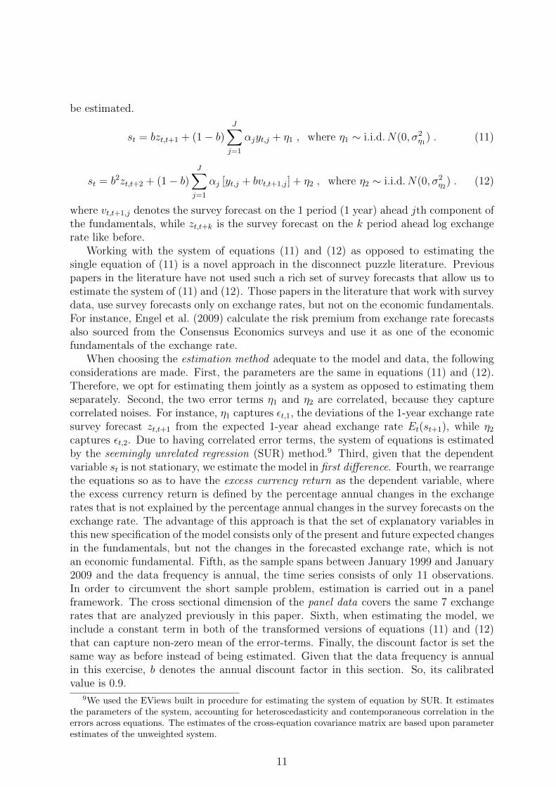
Working with the system of equations (11) and (12) as opposed to estimating thesingle equation of (11) is a novel approach in the disconnect puzzle literature. Previouspapers in the literature have not used such a rich set of survey forecasts that allow us toestimate the system of (11) and (12). Those papers in the literature that work with surveydata, use survey forecasts only on exchange rates, but not on the economic fundamentals.For instance, Engel et al. (2009) calculate the risk premium from exchange rate forecastsalso sourced from the Consensus Economics surveys and use it as one of the economicfundamentals of the exchange rate.

When choosing the estimation method adequate to the model and data, the followingconsiderations are made. First, the parameters are the same in equations (11) and (12).Therefore, we opt for estimating them jointly as a system as opposed to estimating themseparately. Second, the two error terms η1 and η2 are correlated, because they capturecorrelated noises. For instance, η1 captures εt,1, the deviations of the 1-year exchange ratesurvey forecast zt,t+1 from the expected 1-year ahead exchange rate Et(st+1), while η2captures εt,2. Due to having correlated error terms, the system of equations is estimatedby the seemingly unrelated regression (SUR) method.9 Third, given that the dependentvariable st is not stationary, we estimate the model in first difference. Fourth, we rearrangethe equations so as to have the excess currency return as the dependent variable, wherethe excess currency return is defined by the percentage annual changes in the exchangerates that is not explained by the percentage annual changes in the survey forecasts on theexchange rate. The advantage of this approach is that the set of explanatory variables inthis new specification of the model consists only of the present and future expected changesin the fundamentals, but not the changes in the forecasted exchange rate, which is notan economic fundamental. Fifth, as the sample spans between January 1999 and January2009 and the data frequency is annual, the time series consists of only 11 observations.In order to circumvent the short sample problem, estimation is carried out in a panelframework. The cross sectional dimension of the panel data covers the same 7 exchangerates that are analyzed previously in this paper. Sixth, when estimating the model, weinclude a constant term in both of the transformed versions of equations (11) and (12)that can capture non-zero mean of the error-terms. Finally, the discount factor is set thesame way as before instead of being estimated. Given that the data frequency is annualin this exercise, b denotes the annual discount factor in this section. So, its calibratedvalue is 0.9.

9We used the EViews built in procedure for estimating the system of equation by SUR. It estimatesthe parameters of the system, accounting for heteroscedasticity and contemporaneous correlation in theerrors across equations. The estimates of the cross-equation covariance matrix are based upon parameterestimates of the unweighted system.

11

After all these considerations, the system we estimate is:

st−st−1−0.9 [zt,t+1 − zt−1,t] = α0,1+0.1J∑j=1

αj(yt,j−yt−1,j)+λ1 , where λ1 ∼ i.i.d.N(0, σ2λ1

) .

(13)

st−st−1−0.92 [zt,t+2 − zt−1,t+1] = α0,2+0.1J∑j=1

αj [(yt,j − yt−1,j) + 0.9(vt,t+1,j − vt−1,t,j)]+λ2 ,

(14)where λ2 ∼ i.i.d.N(0, σ2

λ2) .

The important economic determinants of exchange rate can be found by estimatingthe system of equations of (13) and (14) on a wide range of economic indicators. Theeconomic indicators that are considered to be potential exchange rate fundamentals are theGDP growth rate, budget deficit relative to GDP, current account, inflation rate, shortterm interest rate, long term interest rate and oil price. More precisely, the potentialfundamentals are defined as the difference between the domestic and the foreign values ofthe above variables with the exception of global oil price.

As a first step, we estimate different specifications of the model that include onlyone of the economic variables. Than, we select those economic variables to the indexof fundamentals that are assigned significant coefficients in the first step. Finally, theweights αj for the components of the fundamental index are obtained by estimating thefinal model that controls for all the selected components. This way, we build the finalmodel with the bottom up approach. The economic fundamentals in the final model arethe GDP growth rate, the budget deficit relative to GDP, the short and long interest ratesand oil price. Surprisingly, neither inflation rate, nor current account are found significantdeterminants of the exchange rate in the first step. Therefore, they are not included inthe final model.

Regarding the oil price, we estimate its effect the following way. We re-estimate themodels that control for only one economic variable and its forecast, but this time we alsoinclude the oil price and its forecast. These estimates are carried out not only on paneldata, but also for each county separately, and for panels of various groups of countries.These estimates suggest that oil is an important determinant of the exchange rate only forsome oil producing countries, like Canada, Norway and the UK. The estimated coefficientsof oil are very close to each other for these three countries. Therefore, we restrict thecoefficient of oil in the final regression model to be the same for the 3 countries, whilezero for the rest of the countries.

The results obtained with the final model are presented in Table 4. It shows that fourof the five economic indicators are assigned statistically significant weights and each of theweights are significant also in economic terms. For instance, if the difference between thedomestic and the foreign annual GDP growth rate increases by one percentage point fromone year to another, then the appreciation of the domestic currency is 0.73 percentagehigher for that year, ceteris paribus.

The goodness of fit measured by the R2s are 0.32 and 0.45 for equations (13) and(14), respectively. These values of R2s indicate fairly good fit, especial in the light ofthe previous literature. Evans (2010) writes ”In fact, my empirical results indicate thatbetween 20 and 30 percent of the variance in excess currency returns over one- and two-month horizons can be linked back to developments in the macroeconomy. This level

12

of explanatory power is an order of magnitude higher than that found in traditionalmodels - even the newly developed monetary models incorporating central banks reactionfunctions.” Although the R2s of this paper are higher than those in Evans (2010), wecannot say that the results in this paper are stronger. When comparing the results ofEvans (2010) and those of this paper, the following considerations should be made. First,Evans (2010) defines the excess currency return differently, than this paper. There, it is thereturn not explained by the interest rate differential, while it is the return not explainedby survey forecasts on exchange rate. Second, another essential difference between Evans(2010) and this paper, is that the former investigates one-month and two-month returns,while the returns in this paper are annual. It is worth noting that Evans (2010) tackleda more challenging problem as it is more difficult to explain exchange rate movements onthe shorter than one year horizon.

In order to demonstrate the importance of working with the system of equationsof (13) and (14), we estimate also the single equation model of (13). The results arepresented in Table 5. As it is apparent from the comparison of Table 4 and Table 5, onecan obtain more precise estimates by the system. And also, more economic indicatorsprove to be significant determinants of the exchange rate with the system, than with thesingle equation approach. So, exploiting the link between forecasted exchange rate andforecasted economic fundamentals helps us to identify the link between exchange rate andeconomic fundamentals.

4 Conclusion

For a long while, the main means of evaluating exchange rate models was to compare theirout-of-sample forecasting performances. This paper has proposed a new test for the assetpricing model of exchange rate. The primary motivation for proposing an alternative testto the traditional one is that it is found by the recent literature that it is too harsh torequire the exchange rate models to outperform the random walk at forecasting. As itis argued by Engel and West (2005), it is almost impossible to come up with a betterforecast than the random walk. They point out that if the fundamentals have a persistentprocess and the discount factor is high enough, then the exchange rate follows a processthat is indistinguishable from the random walk on the usual sample sizes. For this reason,even if the traditional test formally rejects the asset pricing model against the randomwalk model, the former can still be the right one.

The test proposed in this paper uses survey data on exchange rate expectations. Itexamines whether the way market analysts generate their forecasts is closer to the oneimplied by the asset pricing model, or to that implied by the naive random walk model.The models differ in their predictions on the term-structure of forecasts. The forecast isan exponential function of the forecast horizon in the general asset pricing model, whileit is constant in the random walk model given that under the random walk assumptionno change is expected in the exchange rate in any horizon.

The remarkable result of the proposed test is that the asset pricing model has signif-icantly better fit on survey data, than the random walk. The relative goodness of fit ofthe competing models is found to be robust to whether it is measured in-sample or out-of-sample. We can interpret this result as follows. What the representative professionalexchange rate forecaster has in mind about the exchange rate can be better represented

13

by the asset pricing model. If we believe that the model used by the forecasters is iden-tical to the data generating process of the exchange rate, then the asset pricing modelcaptures better not only the way in which the expectations are formed, but also the waythe exchange rate is actually determined.

This paper investigated also whether some commonly considered economic fundamen-tals are linked to the exchange rate in a way consistent with the asset pricing model.The novelty in the applied empirical approach is to use not only historical data, but alsosurvey forecasts both on the exchange rate and on its potential economic fundamentals toidentify the significant determinants of the exchange rate. With these rich data, we foundthat GDP, budget deficit and oil price together with the short and long interest rates areimportant drivers of the exchange rate. It is also a remarkable result that these economicfundamentals can explain 32 and 45 percent of the variance in excess currency returnsover the one-year horizon. These values are comparable in magnitude to those obtainedby Evans (2010), whose model and economic fundamentals can explain between 20 and30 percent of the variance in excess currency returns over one- and two-month horizons.

14

AppendixIn this Appendix we show that under the assumed process of the fundamental xt of (2),the k period-ahead expected log exchange rate Et(st+k) is given by equation (3) in thereduced form asset-pricing model of (1).

First, it is important to note that matrix F is the transition matrix of vector ξt.

ξt =

xtxt−1

1

= Fξt−1 . (15)

This implies thatEt(ξt+j) = F jξt . (16)

We know that

Et(st+k) = (1− b)∞∑j=0

bjEt(xt+k+j) . (17)

Note from (16) that Et(xt+k+j) is given by the first component of the vector F k+jξt.Now consider

(1− b)∞∑j=0

bjF k+jξt = (1− b)F k

(∞∑j=0

bjF j

)ξt . (18)

The first component of this vector is Et(st+k). By formula [1.2.46] in Hamilton (1994),the matrix sum in the parenthesis is equal to

(I − bF )−1 . (19)

provided that the eigenvalues of F are all less than b−1 in absolute value.10 In sum, thefirst component of the vector (1− b)F k(I − bF )−1ξt is precisely Et(st+k) for k > 0.

10This eigenvalue condition is satisfied by all of the estimates in this paper.

15

References

Burda, M. C., Gerlach, S., 1993. Exchange rate dynamics and currency unification: Theostmark-dm rate. Empirical Economics 18 (3), 417–29.

De Grauwe, P., Dewachter, H., Veestraeten, D., 1999. Explaining recent europeanexchange-rate stability. International Finance 2 (1), 1–31.

Engel, C., Wang, J., Wu, J., 2009. Can long-horizon forecasts beat the random walk underthe engel-west explanation? Globalization and monetary policy institute working paper,Federal Reserve Bank of Dallas.

Engel, C., West, K. D., 2005. Exchange rates and fundamentals. Journal of PoliticalEconomy 113 (3), 485–517.

Evans, M. D., January 2010. Order flows and the exchange rate disconnect puzzle. Journalof International Economics 80 (1), 58–71.

Frankel, J. A., Froot, K. A., 1987. Using survey data to test standard propositions re-garding exchange rate expectations. American Economic Review 77 (1), 133–53.

Frenkel, J. A., Mussa, M. L., 1980. The efficiency of foreign exchange markets and mea-sures of turbulence. American Economic Review 70 (2), 374–81.

Gardeazabal, J., Regulez, M., Vazquez, J., 1997. Testing the canonical model of exchangerates with unobservable fundamentals. International Economic Review 38 (2), 389–404.

Goffe, W. L., Ferrier, G. D., Rogers, J., 1994. Global optimization of statistical functionswith simulated annealing. Journal of Econometrics 60 (1-2), 65–99.

Hamilton, J. D., 1994. Time Series Analysis. Princeton Univ. Press.

Krugman, P., 1992. Exchange rate in a currency band: A sketch of the new approach. In:Krugman, P., Miller, M. (Eds.), Exchange Rate Targets and Currency Bands. NBERBooks. National Bureau of Economic Research, Inc, pp. 9–14.

Lieli, R. P., Naszodi, A., 2013. Blame the discount factor no matter what the fundamentalsare, unpublished manuscript.

Meese, R. A., Rogoff, K., 1983. Empirical exchange rate models of the seventies: Do theyfit out of sample? Journal of International Economics 14 (1-2), 3–24.

Obstfeld, M., Rogoff, K., Jul. 2000. The six major puzzles in international macroeco-nomics: Is there a common cause? Nber working papers, National Bureau of EconomicResearch, Inc.

16

Table 1: Parameter Estimates of the Asset Pricing Model

CADUSD

USDEUR

USDGBP

JPYUSD

CHFEUR

NOKEUR

SEKEUR

b 99.13% 99.13% 99.13% 99.13% 99.13% 99.13% 99.13%ϕ1 0.1626 0.0589 1.0878 0.6684 0.4289 0.5513 0.8589std.dev. 0.1758 0.0491 0.0172 0.0301 0.5911 0.2094 0.0114ϕ2 0.8173 0.911 -0.0993 0.2459 0.5219 0.2454 0.0399std.dev. 0.174 0.0488 0.0171 0.0254 0.5732 0.1765 0.0108α 0.0046 0.0053 0.0057 0.4015 0.0209 0.4251 0.2194std.dev. 0.0006 0.0008 0.0007 0.0699 0.0089 0.0792 0.0103σx 0.0911 0.1759 0.0587 0.3691 0.0683 0.4125 0.1825std.dev. 0.012 0.0157 0.0047 0.0571 0.0274 0.074 0.0157σz,k=0.25Y 0.0131 0.0209 0.013 0.0317 0.0088 0.0172 0.0094std.dev. 0.0012 0.0016 0.0009 0.0029 0.0009 0.0021 0.0008σz,k=1Y 0.0151 0.0402 0.0182 0.0564 0.0143 0.0255 0.0151std.dev. 0.0015 0.0038 0.0016 0.0077 0.0017 0.004 0.0016σz,k=2Y 0.0158 0.0446 0.0228 0.0625 0.0178 0.0233 0.0176std.dev. 0.0014 0.0052 0.0019 0.0081 0.0022 0.0033 0.0017ρz,0.25Y ,1Y 0.853 0.8572 0.77 0.8997 0.8469 0.8976 0.6814std.dev. 0.0276 0.026 0.0359 0.0223 0.0345 0.0253 0.0662ρz,0.25Y ,2Y 0.614 0.7657 0.5623 0.8191 0.668 0.8152 0.5245std.dev. 0.092 0.0448 0.0679 0.046 0.0755 0.0622 0.0871ρz,1Y ,2Y 0.6502 0.9365 0.7835 0.9644 0.8933 0.9174 0.9439std.dev. 0.0952 0.0194 0.0443 0.0109 0.0304 0.0285 0.0138log likelihood 1371 1128 1287 1061 1574 1360 1521

Note: the covariance matrix of the parameter estimates (that is used to calculate the reportedstandard deviations (std.dev.)) is calculated as the outer product of the gradient.

17

Table 2: Parameter Estimates of the Random Walk Model

CADUSD

USDEUR

USDGBP

JPYUSD

CHFEUR

NOKEUR

SEKEUR

b 99.13% 99.13% 99.13% 99.13% 99.13% 99.13% 99.13%ϕ1 1 1 1 1 1 1 1ϕ2 0 0 0 0 0 0 0α 0 0 0 0 0 0 0σx 0.0224 0.0333 0.0267 0.0346 0.0097 0.0174 0.0143std.dev. 0.0017 0.0018 0.0013 0.0019 0.0007 0.001 0.001σz,k=0.25Y 0.0157 0.0254 0.0141 0.0278 0.0105 0.0144 0.0165std.dev. 0.0014 0.0016 0.0008 0.0019 0.0009 0.0009 0.0019σz,k=1Y 0.0304 0.0609 0.0272 0.0488 0.0202 0.0246 0.0324std.dev. 0.0029 0.0042 0.002 0.0036 0.0023 0.0019 0.0041σz,k=2Y 0.0383 0.0817 0.0389 0.062 0.0286 0.0266 0.0404std.dev. 0.0038 0.0058 0.0032 0.004 0.0032 0.0019 0.0052ρz,0.25Y ,1Y 0.8266 0.8855 0.7619 0.8253 0.9029 0.8012 0.927std.dev. 0.0305 0.0194 0.0376 0.0272 0.0189 0.0283 0.0165ρz,0.25Y ,2Y 0.7658 0.8286 0.6226 0.6408 0.7989 0.6465 0.8928std.dev. 0.042 0.0289 0.0562 0.0588 0.0468 0.0651 0.0268ρz,1Y ,2Y 0.9724 0.9789 0.9186 0.9274 0.9469 0.906 0.9882std.dev. 0.0058 0.0034 0.0135 0.0138 0.0178 0.0183 0.0036log likelihood 1297 1067 1223 1031 1521 1327 1431

Note: the same as below Table 1.

18

Table 3: Parameter Estimates of the Asset Pricing Model on the Restricted Sample

CADUSD

USDEUR

USDGBP

JPYUSD

CHFEUR

NOKEUR

SEKEUR

b 99.13% 99.13% 99.13% 99.13% 99.13% 99.13% 99.13%ϕ1 0.0638 0.1608 0.2745 0.8384 0.3162 0.7233 0.6215std.dev. 0.319 0.5819 0.3412 0.0033 0.4538 0.0043 0.0075ϕ2 0.9196 0.8121 0.7046 0.165 0.6193 0.1805 0.2555std.dev. 0.3166 0.573 0.3369 0.0053 0.4341 0.0041 0.0073α 0.0039 0.0046 0.0102 -0.0175 0.0274 0.2014 0.2668std.dev. 0.0011 0.0017 0.0025 0.0126 0.011 0.0005 0.0007σx 0.0846 0.162 0.1079 0.0051 0.0859 0.2048 0.2209std.dev. 0.0261 0.0523 0.023 0.002 0.0319 0.0008 0.0008σz,k=1Y 0.0179 0.0412 0.0183 0.0437 0.014 0.021 0.015std.dev. 0.0027 0.0038 0.0017 0.0032 0.0016 0.0008 0.0001σz,k=2Y 0.0169 0.0459 0.0228 0.0513 0.0177 0.0207 0.0175std.dev. 0.0011 0.005 0.0018 0.004 0.0021 0.0001 0ρz,1Y ,2Y 0.8145 0.9432 0.7899 0.905 0.889 0.8727 0.9433std.dev. 0.0297 0.0171 0.0433 0.0188 0.0293 0.007 0.0013RMSE AP 0.0214 0.0525 0.0192 0.0867 0.0086 0.0237 0.0103RMSE RW 0.0288 0.0752 0.0231 0.0904 0.013 0.0242 0.032

Notes: The restricted sample does not cover the 3-month forecasts. RMSE AP and RMSE RWmeasure the out-of-sample fit of the asset pricing model and the random walk model on the

3-month survey forecasts, respectively.

19

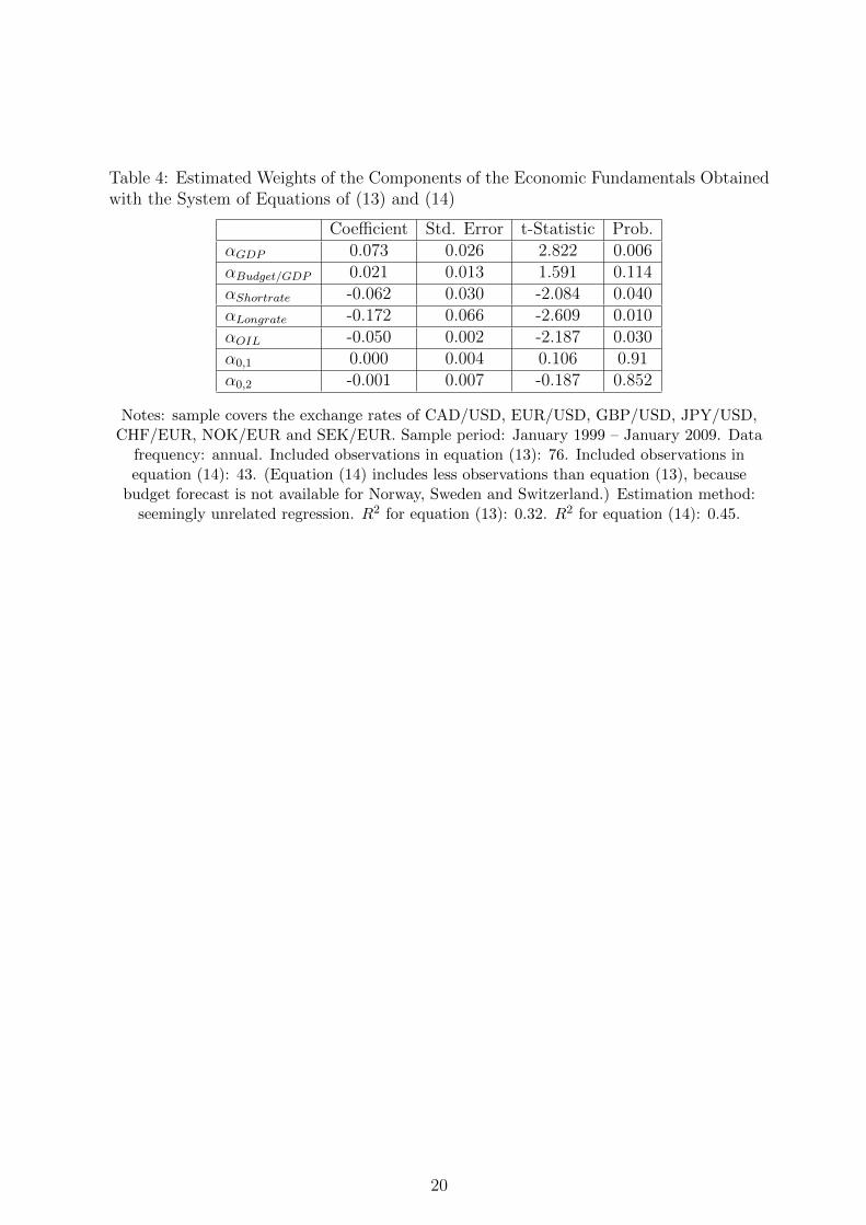
Table 4: Estimated Weights of the Components of the Economic Fundamentals Obtainedwith the System of Equations of (13) and (14)

Coefficient Std. Error t-Statistic Prob.αGDP 0.073 0.026 2.822 0.006αBudget/GDP 0.021 0.013 1.591 0.114αShortrate -0.062 0.030 -2.084 0.040αLongrate -0.172 0.066 -2.609 0.010αOIL -0.050 0.002 -2.187 0.030α0,1 0.000 0.004 0.106 0.91α0,2 -0.001 0.007 -0.187 0.852

Notes: sample covers the exchange rates of CAD/USD, EUR/USD, GBP/USD, JPY/USD,CHF/EUR, NOK/EUR and SEK/EUR. Sample period: January 1999 – January 2009. Data

frequency: annual. Included observations in equation (13): 76. Included observations inequation (14): 43. (Equation (14) includes less observations than equation (13), because

budget forecast is not available for Norway, Sweden and Switzerland.) Estimation method:seemingly unrelated regression. R2 for equation (13): 0.32. R2 for equation (14): 0.45.

20

Table 5: Estimated Weights of the Components of the Economic Fundamentals Obtainedwith Equation (13)

Coefficient Std. Error t-Statistic Prob.αGDP 0.060 0.032 1.907 0.061αBudget/GDP 0.018 0.017 1.020 0.311αShortrate -0.035 0.038 -0.909 0.367αLongrate -0.266 0.086 -3.105 0.003αOIL -0.006 0.003 -1.875 0.065α0,1 0.001 0.004 0.126 0.900

Notes: sample covers the exchange rates of CAD/USD, EUR/USD, GBP/USD, JPY/USD,CHF/EUR, NOK/EUR and SEK/EUR. Sample period: January 1999 – January 2009. Datafrequency: annual. Included observations in the : 76. Estimation method: least squares. R2

for equation (13): 0.33.

21