Testing the Data Assimilation Capability of the Profiler

ARL-TR-7601 ● FEB 2016

US Army Research Laboratory

Testing the Data Assimilation Capability of the Profiler Virtual Module

by Patrick A Haines, Jeffrey A Smith, Brian P Reen, James L Cogan, David R Stauffer, David J Epler, and RW Hornbaker Approved for public release; distribution is unlimited.

NOTICES

Disclaimers

The findings in this report are not to be construed as an official Department of the Army position unless so designated by other authorized documents. Citation of manufacturer’s or trade names does not constitute an official endorsement or approval of the use thereof. Destroy this report when it is no longer needed. Do not return it to the originator.

ARL-TR-7601 ● FEB 2016

US Army Research Laboratory

Testing the Data Assimilation Capability of the Profiler Virtual Module

by Patrick A Haines, Jeffrey A Smith, Brian P Reen, and James L Cogan Computational and Information Sciences Directorate, ARL and

David R Stauffer Pennsylvania State University, Department of Meteorology, University Park, PA

David J Epler CACI International, Lawton, OK

RW Hornbaker SpecPro Technical Services, Systems Integration (SSI), San Antonio, TX Approved for public release; distribution is unlimited.

ii

REPORT DOCUMENTATION PAGE Form Approved OMB No. 0704-0188

Public reporting burden for this collection of information is estimated to average 1 hour per response, including the time for reviewing instructions, searching existing data sources, gathering and maintaining the data needed, and completing and reviewing the collection information. Send comments regarding this burden estimate or any other aspect of this collection of information, including suggestions for reducing the burden, to Department of Defense, Washington Headquarters Services, Directorate for Information Operations and Reports (0704-0188), 1215 Jefferson Davis Highway, Suite 1204, Arlington, VA 22202-4302. Respondents should be aware that notwithstanding any other provision of law, no person shall be subject to any penalty for failing to comply with a collection of information if it does not display a currently valid OMB control number. PLEASE DO NOT RETURN YOUR FORM TO THE ABOVE ADDRESS.

1. REPORT DATE (DD-MM-YYYY)

February 2016 2. REPORT TYPE

Final 3. DATES COVERED (From - To)

2015 January–August 4. TITLE AND SUBTITLE

Testing the Data Assimilation Capability of the Profiler Virtual Module 5a. CONTRACT NUMBER

5b. GRANT NUMBER

5c. PROGRAM ELEMENT NUMBER

6. AUTHOR(S)

Patrick A Haines, Jeffrey A Smith, Brian P Reen, James L Cogan, David R Stauffer, David A Epler, and RW Hornbaker

5d. PROJECT NUMBER

5e. TASK NUMBER

5f. WORK UNIT NUMBER

7. PERFORMING ORGANIZATION NAME(S) AND ADDRESS(ES)

US Army Research Laboratory Computational and Information Sciences Directorate Battlefield Environment Division (ATTN: RDRL-CIE-M) White Sands Missile Range, NM 88002-5501

8. PERFORMING ORGANIZATION REPORT NUMBER

ARL-TR-7601

9. SPONSORING/MONITORING AGENCY NAME(S) AND ADDRESS(ES)

10. SPONSOR/MONITOR'S ACRONYM(S)

11. SPONSOR/MONITOR'S REPORT NUMBER(S)

12. DISTRIBUTION/AVAILABILITY STATEMENT

Approved for public release; distribution is unlimited. 13. SUPPLEMENTARY NOTES 14. ABSTRACT

This report presents the methodology and results of an analysis of the accuracy of meteorological computer messages derived from 1) a Profiler Virtual Module (PVM) using its data assimilation (DA) capability as compared with 2) a PVM with its DA capability turned off. The PVM’s Nowcasting accuracy was compared to the currently fielded artillery meteorological (MET) system, the Computer Meteorological Data-Profiler is described in an earlier technical report in 2014 by J Cogan, P Haines, J Seik, and A Wetmore, ARL-TR-7149; however, those comparisons were based on testing in which both systems relied only on Global Forecast System data for initialization and did not include assimilation of World Meteorological Organization data. In this report, accuracy is defined in terms of the closeness of the PVM’s Nowcast fields to coincident upper air rawinsondes (soundings) obtained from Yuma Proving Ground (YPG), Arizona. The YPG soundings made at the YPG MET station were launched and assimilated by one of the PVMs between 1200 and 0000 Coordinated Universal Time (UTC). The assimilated soundings were made every 3 h and noningested soundings were used for ground truth. The noningested YPG MET soundings were launched at intermediate times, and noningested soundings were made at 2 other YPG locations that were launched at varying times between 1200 and 0000 UTC.

15. SUBJECT TERMS

data assimilation, profiler virtual module, nudging, PVM, DA, weather research and forecasting, WRF

16. SECURITY CLASSIFICATION OF: 17. LIMITATION OF ABSTRACT

UU

18. NUMBER OF PAGES

56

19a. NAME OF RESPONSIBLE PERSON

Patrick Haines a. REPORT

Unclassified b. ABSTRACT

Unclassified c. THIS PAGE

Unclassified 19b. TELEPHONE NUMBER (Include area code)

(575) 678-5593 Standard Form 298 (Rev. 8/98) Prescribed by ANSI Std. Z39.18

Approved for public release; distribution is unlimited.

iii

Contents

List of Figures iv

List of Tables vi

Acknowledgments vii

1. Introduction 1

1.1 Background on DA 4

1.2 PVM WRF DA 8

2 Methodology and Test Procedures 11

2.1 Testing Profiler DA 11

2.2 Limitations to the Testing 11

2.3 Soundings Test Procedure 13

2.4 PVM Results 15

2.4.1 Data Analysis Methodology 15

2.4.2 Comparison Results 16

3. Summary and Conclusions 28

4. References and Notes 32

Appendix A. Required Additional Miltope Configuration and Scripts 35

Appendix B. Cross-Reference of Samples by Date, Time, and Location 41

Bibliography 43

List of Symbols, Abbreviations, and Acronyms 44

Distribution List 46


iv

List of Figures

Fig. 1 Overall timeline for one test event. The GFS was initialized with 12 Z data on the preceding day and run through its 144 h forecast cycle. The resulting GFS forecast data were disseminated several hours later and placed on the Army data folder. Those GFS data were downloaded and used to initialize the PVM. At 00 Z, the data receipt for the PVM laptop with DA was turned on and left on for the rest of the test period. The 00 Z WMO data were received and assimilated in the period from 00 Z to 12 Z, but there was little lingering effect on the PVM by 12 Z on the next day. ......................................................................................3

Fig. 2 Overall timeline for one test day. WMO soundings (including the YPG MET station sounding) and surface data were received at and somewhat after 12 Z at which time the data entered the DA cycle. Later, at 15 Z, a new YPG sounding was made and it was soon afterwards received by the PVM. It then too entered the PVM DA cycle. This process was also repeated at 18 Z and 21 Z. .......................3

Fig. 3 Decrease of model error with time when nudging with various nudging weights and assuming that all of the physical tendency terms are zero .......................................................................................................10

Fig. 4 YPG soundings sites. Building 3555, Tower 31, and Tower M soundings were used in this study. .......................................................12

Fig. 5 Overall timeline for one test event. The GFS was initialized with 12 Z data on the preceding day and run through its 144 h forecast cycle. The resulting GFS forecast data were disseminated several hours later and placed in the Army data folder. That set of GFS data was downloaded and used to initialize the PVM a little before 21 Z or 22 Z. Up to 00 Z no data were received by either PVM system. At 00 Z, METCMs were generated on both systems and compared. The data receipt for the PVM laptop with DA was then turned on and left on for the rest of the test period. That meant that the 00 Z WMO data were received and assimilated in the period from 00 Z to 04 Z; however, comparisons of METCMs generated at 12 Z the next day against verifying soundings show that there was very little lingering effect from the DA. The details on assimilated and verifying soundings are shown in Fig. 6. ...14

Fig. 6 Overall timeline for one test day. WMO soundings (including the YPG Building 3555 sounding) and surface data were received at and somewhat after 12 Z at which time the data entered the DA cycle. Later, at 15 Z, 18 Z, and 21 Z new YPG soundings were made (denoted by the blue boxes) and they shortly thereafter entered PVM’s DA cycle. At other hours independent verifying soundings (VS) were made as denoted by the gold colored boxes.........................................15


v

Fig. 7 Mean Absolute Density Error values: all stations with DA (darker blue), all stations without DA (violet). With DA: Station R only (red), Stations S and T only (light green). Without DA: Station R only (light blue), Stations S and T only (orange). .................................................17

Fig. 8 Mean Absolute Density Error values for Station R only: with DA (blue), without DA (red) ......................................................................18

Fig. 9 Mean Absolute Density Error values for Stations S and T only: with DA (blue), without DA (red) ...............................................................19

Fig. 10 Temperature Error Values: all stations with DA (darker blue), all stations without DA (violet). With DA: Station R only (red), Stations S and T only (light green). Without DA: Station R only (light blue), Stations S and T only (orange).............................................................20

Fig. 11 Temperature Error Values for Station R only: with DA (blue), without DA (red) ...............................................................................................21

Fig. 12 Temperature Error Values for Stations S and T only: with DA (blue), without DA (red) ..................................................................................22

Fig. 13 Mean Absolute Pressure Error Values: all stations with DA (Darker Blue), all stations without DA (Violet). With DA: Station R only (red), Stations S and T only (light green). Without DA: Station R only (light blue), Stations S and T only (orange). .................................................23

Fig. 14 Mean Absolute Pressure Error values for Station R only: with DA (blue), without DA (red) ......................................................................24

Fig. 15 Mean Absolute Pressure Error values for Stations S and T only: with DA (blue), without DA (red) ...............................................................25

Fig. 16 Vector Wind Mean Absolute Error values: all stations with DA (darker blue), all stations without DA (violet). With DA: Station R only (red), Stations S and T only (light green). Without DA: Station R only (light blue), Stations S and T only (orange). .................................................26

Fig. 17 Vector Wind Mean Absolute Error values for Station R only: with DA (blue), without DA (red) ......................................................................27

Fig. 18 Vector Wind Mean Absolute Error values for Stations S and T only: with DA (blue), without DA (red) .......................................................28


vi

List of Tables

Table 1 YPG sounding observation sites ..........................................................12

Table 2 Cross reference of samples by study date (all 2015) and study time for both with and without DA cases. The number within the cell indicates the number of model-sounding pairs available to compare at that date and time. ...............................................................................................16

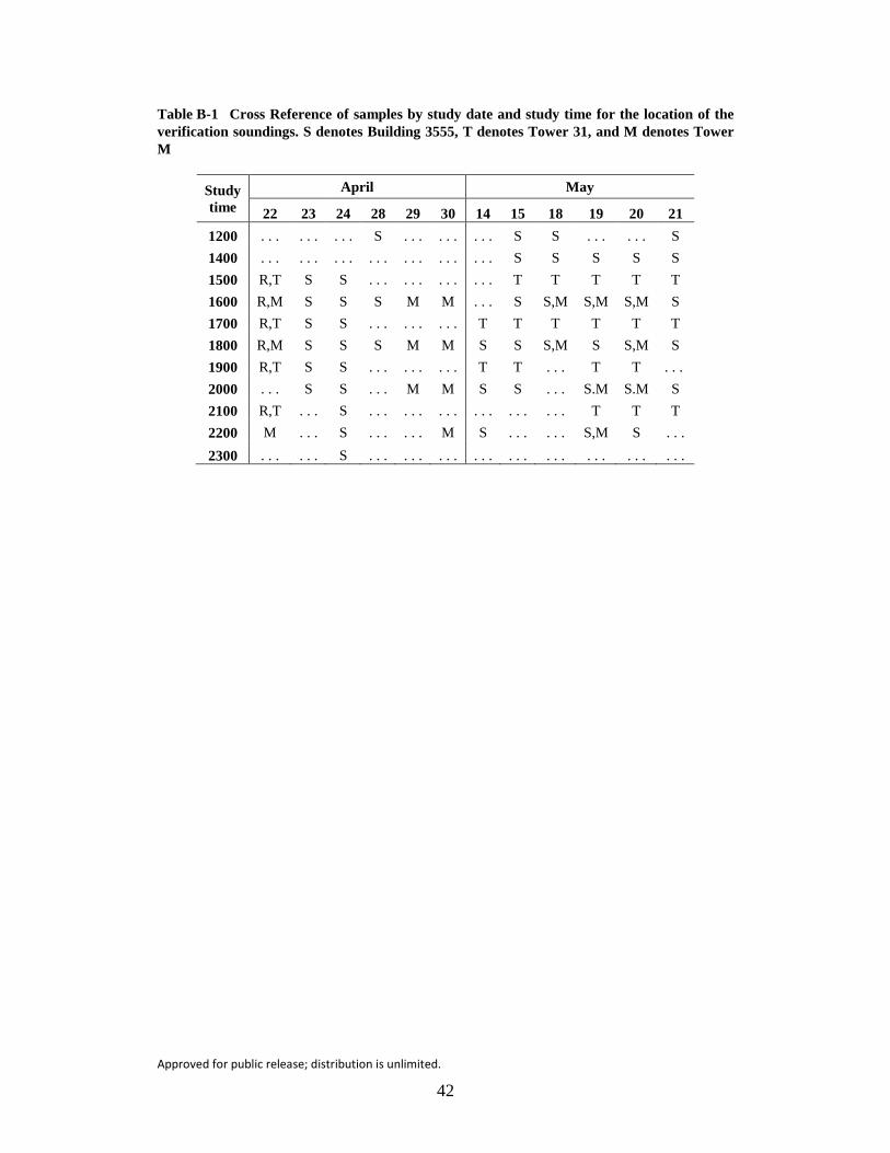
Table B-1 Cross Reference of samples by study date and study time for the location of the verification soundings. S denotes Building 3555, T denotes Tower 31, and M denotes Tower M .......................................42


vii

Acknowledgments

The authors would like to acknowledge Ms Gina Selga for generating meteorological (MET) messages on a lot of early mornings at 12 Zulu (Z) (0600 MDT). These messages showed that the assimilating and nonassimilating Profiler Virtual Module system’s messages were in close agreement just prior to assimilation of the 12 Z World Meteorological Organization soundings (including Yuma Proving Ground [YPG], Arizona).

This study would not have been possible without the cooperation of the YPG MET team and in particular Mr Mark Hendricksen who provided the sounding launch site and time information so that the MET messages could be generated at the US Army Research Laboratory (ARL) Artillery Test Laboratory in real time. They also provided all of the YPG MET soundings in a convenient format.

We would like to thank Mr Edward Creegan of ARL who also generated some of the early morning 12 Z MET messages.

Special thanks to Sherry Larson for her usual exemplary editing of this report.


viii

INTENTIONALLY LEFT BLANK.


1

1. Introduction

The Profiler Virtual Module (PVM) is a Numerical Weather Prediction (NWP) Nowcasting System currently being fielded by the US Army. It will be used to produce timely meteorological information for artillery trajectory calculations. The PVM receives Global Forecast System (GFS) global model weather prediction data via satellite transmission (Global Broadcast System [GBS]) or over the tactical Internet at a Tactical Operations Center. It also receives World Meteorological Organization (WMO) upper air sounding and surface data via GBS. GFS data are used to initialize the PVM’s Weather Research and Forecasting (WRF) Nowcasting System. The PVM version used in this study consisted of a triple-nested configuration: Domain 1 is a 101 × 101 grid with a 36-km grid spacing, Domain 2 is a 139 × 139 grid with a 12-km grid spacing and Domain 3, the finest nested grid, is a 133 × 133 grid with a 4-km grid spacing. The system is designed to provide a continuous stream of highly detailed Nowcasts, defined as gridded meteorological (MET) fields produced by a high-resolution nonhydrostatic mesoscale model continuously assimilating available observations (obs) and staying ahead of the clock to provide timely current meteorological conditions (e.g., Schroeder et al. 2006). The WMO data are assimilated in the Nowcast system to improve overall system accuracy for producing the field artillery MET messages.

This report presents the methodology and results of an analysis of the accuracy of meteorological computer messages (METCMs) derived from 1) a PVM using its data assimilation (DA) capability as compared with 2) a PVM with its DA capability turned off. The PVM’s Nowcasting accuracy was compared to the currently fielded artillery MET system, the Computer Meteorological Data-Profiler (CMD-P) in an earlier report (Cogan et al. 2014). That report showed that the PVM had nearly the same or slightly better accuracy than the CMD-P as related to coincident rawinsonde (sounding) data, but the comparisons were based on testing in which both systems relied only on GFS data for initialization and did not include assimilation of WMO data.

Accuracy is defined in terms of the closeness of the model Nowcast fields to coincident upper air rawinsondes (soundings) obtained from Yuma Proving Ground (YPG), Arizona. YPG soundings at one location were launched and assimilated by one of the PVMs between 1200 and 0000 Coordinated Universal Time (UTC) (also denoted by Zulu [Z]) approximately every 3 h while those at 2 other YPG locations were launched at varying times between 1200 and 0000 UTC and not ingested into the PVM systems. The system accuracy is composited over all sounding locations and times common to both PVM systems: data ingest and time since last data ingest are only defined at one of the 3 YPG sounding locations, while verification is


2

completely independent at the other 2 sounding locations for all verification times. Details on the data assimilated and the test procedure are presented in this report.

Two PVM systems were used and are described in the test and results section in this report. The first system was used as in Cogan et al. (2014), that is, no WMO data were received and used in producing the Nowcast/forecast results and the METCMs shown in that report. The second system, which had direct network connections to a special data folder at the Air Force Weather Agency (AFWA) (AFWA is now the 557th Weather Wing and will be hereafter referred to as the 557th WW), was able to move newly received WMO data from that folder to the test system every 6 min during the testing. The WMO data are typically available every hour at the surface and every 12 h above the surface. However, in this test, the additional YPG rawinsondes used for assimilation were generally available every 3 h between 1200 to 0000 UTC. Details on the PVM modifications necessary to perform this test and the method to query the special folder at the 557th WW are provided in Appendix A of this report. The comparisons were made in terms of the accuracy of the common MET variables of wind, pressure and temperature, and also in terms of the variables most pertinent to artillery accuracy, air density and vector wind error.

Both systems were initialized and started simultaneously with the same data and run for at least 2 30-min Nowcast cycles and typically 4–6 Nowcast cycles to create a baseline comparison without DA. Up to this point, no WMO data were received or used by either system. At this point, METCMs were generated on both systems and immediately compared in order to verify that they had identical or nearly identical initializations. Subsequently, receipt of data was turned on for the DA system and the 2 systems continued with their respective 30-min Nowcast cycles throughout the rest of the test period. During this time, WMO data were received and assimilated in the DA system (see Figs. 1 and 2). Data-ingest locations and times, are shown in Table B-1 in Appendix B.


3

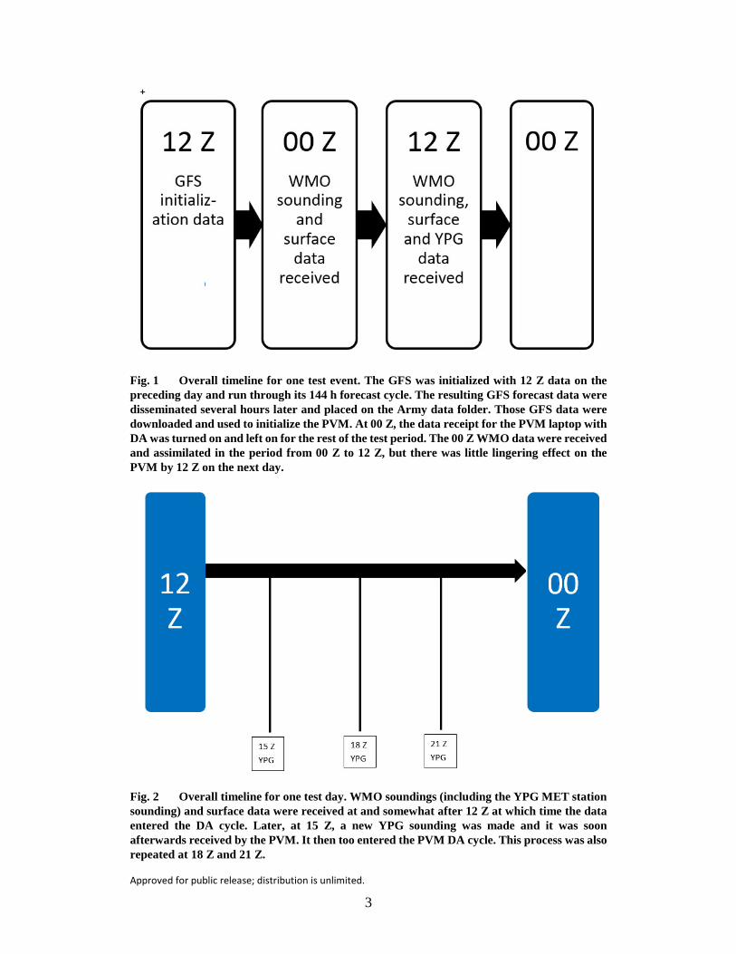
Fig. 1 Overall timeline for one test event. The GFS was initialized with 12 Z data on the preceding day and run through its 144 h forecast cycle. The resulting GFS forecast data were disseminated several hours later and placed on the Army data folder. Those GFS data were downloaded and used to initialize the PVM. At 00 Z, the data receipt for the PVM laptop with DA was turned on and left on for the rest of the test period. The 00 Z WMO data were received and assimilated in the period from 00 Z to 12 Z, but there was little lingering effect on the PVM by 12 Z on the next day.

Fig. 2 Overall timeline for one test day. WMO soundings (including the YPG MET station sounding) and surface data were received at and somewhat after 12 Z at which time the data entered the DA cycle. Later, at 15 Z, a new YPG sounding was made and it was soon afterwards received by the PVM. It then too entered the PVM DA cycle. This process was also repeated at 18 Z and 21 Z.


4

METCMs were generated on both systems at one, 2 or at all 3 locations and at the times when soundings were made. Note that only the YPG MET station sounding was used for sounding ingest by the system. Thus some of the verifications, as in Schroeder et al. (2006), at the time of the ingested sounding, measure the ability of the Nowcast model to use and leverage previous assimilation of data to improve the Nowcast at the time of the current sounding being assimilated. In this way, there is only some independence in the verification data. However, for the following one, 2 or 3 h after ingest time at the data ingest location, the sounding directly affects the Nowcast, and the verification is now measuring the “fit to the data”. At the other 2 sounding locations, for all sounding times, the verification is completely independent since these data were not assimilated.

The intent of this study is to quantify the impact of assimilating WMO obs on PVM system accuracy. The data used included both surface and sounding obs; the soundings have a more significant impact because they cover the depth of the troposphere and extend into the stratosphere. Meanwhile, the surface obs—though much more numerous—have a direct or indirect impact that is typically limited to the depth of the atmospheric boundary layer (e.g., Reen and Stauffer 2010). The depth of the atmospheric boundary layer varies widely over the test region but generally peaks at approximately 1,000 m in mid-afternoon; however, at times it may be significantly higher in a desert environment such as YPG. It was beyond the scope of this study to restrict use to either surface or sounding obs.

1.1 Background on DA

Nearly all objective analysis/DA methods are generally based on combining a model-generated “first guess” or background (xb) and obs (yo) to produce a gridded analysis of the obs (𝑥𝑥𝑎𝑎) as described by the analysis Eq. 1:

𝑥𝑥𝑎𝑎 = 𝑥𝑥𝑏𝑏 + 𝑊𝑊[𝑦𝑦𝑜𝑜 − 𝐻𝐻(𝑥𝑥𝑏𝑏)] , (1)

where yo –H(xb) is the “observation increment” or “innovation”, and H is the obs operator that performs the necessary interpolation and transformation from model variables to obs space. Details on how the model and obs are combined vary among the methods (e.g., Kalnay 2003; Warner 2011). For example, the weight, W, applied to the innovation can be a simple function based on distance between the obs and model grid cell (e.g., Cressman successive scan or traditional nudging), or based on minimizing the analysis error at each grid point (e.g., optimal interpolation [OI]), or based on model and obs error covariances (e.g., ensemble Kalman filter [EnKF]). The 𝑥𝑥𝑎𝑎 may also be determined by minimizing a cost function that measures the “distance” between the analysis and both the obs and model background, scaled by the obs error covariance and model background error covariance, respectively (e.g.,


5

3-dimensional variational [3DVAR]). An innovation-like term can also be included directly within the model itself (nudging), or inserted in a derivative (adjoint) model used to compute the model initial state that produces a forecast that “best fits the observations” (minimizes the cost function) through the forecast/assimilation period (e.g., 4-dimensional variational [4DVAR]). In all of these methods the role of the model is central since it propagates obs information into data-sparse regions and provides dynamic constraints.

DA strategies can be generally divided into intermittent and continuous methods, describing the frequency of data ingest into the model. Preference should be given to methods that generate the least amount of spurious insertion “noise” while enhancing the spinup and accuracy of the model forecast fields. Intermittent methods, such as 3DVAR or EnKF or their combined “hybrid” application, use a prior model forecast as the background for data insertion, then run the model without further data ingest for some time period (typically 1–3 h), and stop the model for another data ingest step before running the model again. This process is repeated throughout the assimilation period. However, these intermittent methods can produce large corrections to the model fields, and produce error/noise “spikes” related to the data insertion (e.g., Fujita et al. 2007), or discontinuities in fields at the seams between update periods (e.g., Bei et al. 2008). Digital filters are often used to reduce insertion errors (Kalnay 2003), but they can also remove realistic high-frequency atmospheric modes that may play a role in the forecast.

On the other hand, continuous DA methods using a strong dynamic constraint (model) include nudging and 4DVAR. Four-dimensional data assimilation (FDDA) or nudging (e.g., Stauffer and Seaman 1994) adds relaxation terms to the model’s prognostic equations to gradually and continuously assimilate data at every time step, which minimizes insertion noise. The innovations can be computed in grid space (analysis nudging) or obs space (obs nudging). The former is intended for coarser-scale grids and synoptic data, while the latter is more suitable for fine-scale grids and asynoptic data (Stauffer and Seaman 1994; Stauffer et al. 2007a, 2007b). Nudging is computationally efficient and easily adaptable to very fine grids, but includes artificial forcing terms while 4DVAR can assimilate non-state variables but generally assumes the model is perfect. Nonlinear discontinuous forcing greatly limits 4DVAR applicability to short assimilation windows, especially on finer scales. 4DVAR is quite computationally expensive requiring many iterations of the forward model and linear adjoint model, and simplified/smooth physics, but even in multi-incremental (dual resolution, inner/outer loop) applications to reduce computation costs, ensembles and 4DVAR are still not being applied to sub-10-km grid length scales as required here for PVM WRF. It must be remembered that these advanced DA methods were developed for larger scales and their application to


6

sub-10-km grid spacings will require further adjustment and approximations that may not improve operational model products for some time even with greater compute power. Nonetheless, hybrid methods that combine, for example, the advantages of EnKF (flow-dependent error covariance and obs weighting) and 3DVAR/4DVAR (e.g., Zhang et al. 2013), or combine the EnKF and obs nudging for time-continuous, gradual corrections, with flow-dependent error covariances and obs weighting (e.g., Lei et al. 2012), are growing in popularity. In this way, the flow-dependent error covariances can improve the static climatological values or ad hoc weighting functions while the EnKF mean is replaced with an analysis with greater dynamic consistency.

There are also a growing number of advanced DA methods and hybrid combinations including a hybrid EnKF 4DVAR that does not require a tangent linear model or adjoint (En4DVAR, Liu et al. 2008), and many methods to define and refine important DA parameters such as background error covariances, localization scales, inflation factors, and so forth. Nonetheless, the fit of the analysis to the obs depends in part on background and obs error covariances and the aforementioned parameters that are increasingly difficult to define for smaller sub-10-km grid length applications.

Therefore, given the much greater cost and complexity of the aforementioned ensemble-based DA methods for sub-10-km grid Nowcasts, the obs nudging FDDA method of Stauffer and Seaman (1994), adapted for the Meteorological Measuring Set-Profiler (MMS-P) (Schroeder et al. 2006), and available in WRF (e.g., Lei et al. 2012; Rogers et al. 2013), is deemed the best current approach for PVM WRF for Nowcasts to support field artillery trajectories.

Nudging is a continuous DA method that applies small, gradual corrections to the model equations every time step around an obs time rather than applying a large single-time correction as an intermittent DA approach. In other words, nudging is a continuous DA since it is applied at every time step over some period, in contrast to other DA techniques that change the model solution only intermittently at certain analysis times. As with any DA methodology there are advantages and disadvantages of the nudging technique. One advantage is that nudging is computationally simple, since it only requires adding an additional tendency term. Another advantage is that it does not require error covariance information used by some other methods such as 3DVAR, or an ensemble of forecasts as with the EnKF. Also, the continuous nature of nudging allows only relatively small changes to be made to the model solution at any given time step. This minimizes data insertion noise and makes it more likely that the model’s physical tendency terms will maintain a higher degree of dynamic balance than when intermittent DA techniques


7

apply much larger changes at a single time step. Nudging also makes it rather simple to incorporate physically based modifications to the functions used to spread information from an obs to the grid (e.g., spreading the influence of surface obs throughout the convective boundary layer due to its well-mixed nature, Reen and Stauffer 2010). One disadvantage of nudging is that it is not able to directly ingest obs of variables not forecasted by the model. For example, radial velocity obs from radar cannot be directly used in nudging because the model does not directly predict radial wind. Other DA methods (e.g., 3DVAR, 4DVAR, and EnKF) often use a forward operator/transformation matrix to ingest these obs. Another disadvantage of traditional nudging is that the weight at which an obs is applied is generally not flow-dependent, but the corrections can propagate throughout the flow and into data-sparse regions. Although there are hybrid, ensemble-based applications of nudging that produce flow-dependent nudging corrections (e.g., Lei et al. 2012), they again require a model ensemble and EnKF, and their computational cost/computing requirements are much larger. Reen (2015) provides further technical background on obs nudging as applied in WRF V3.6.

The PVM WRF employs FDDA through systematic application of obs nudging corrections to gridded fields of MET parameters that are spatially and temporally proximate to obs (e.g., Stauffer and Seaman 1994; Rogers et al. 2013). Obs nudging is a form of Newtonian relaxation wherein artificial tendency terms are introduced into the model to gradually “nudge” the model toward individual obs or asynoptic data (not at the same time); it is also known as station nudging. The other forms of nudging present in WRF (analysis nudging and spectral nudging) relax the model toward synoptic data at the same time as a gridded analysis.

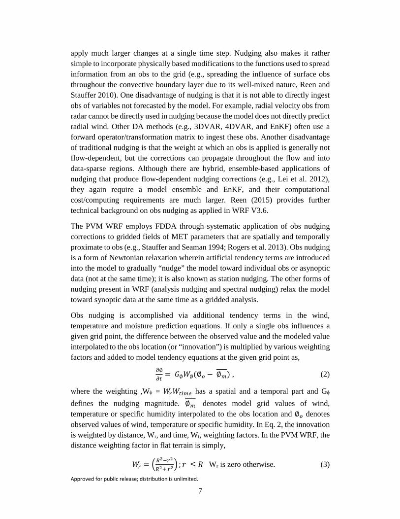
Obs nudging is accomplished via additional tendency terms in the wind, temperature and moisture prediction equations. If only a single obs influences a given grid point, the difference between the observed value and the modeled value interpolated to the obs location (or “innovation”) is multiplied by various weighting factors and added to model tendency equations at the given grid point as,

𝜕𝜕∅𝜕𝜕𝜕𝜕

= 𝐺𝐺∅𝑊𝑊∅(∅𝑜𝑜 − ∅𝑚𝑚) , (2)

where the weighting ,Wφ = 𝑊𝑊𝑟𝑟𝑊𝑊𝜕𝜕𝑡𝑡𝑚𝑚𝑡𝑡 has a spatial and a temporal part and Gφ defines the nudging magnitude. ∅𝑚𝑚 denotes model grid values of wind, temperature or specific humidity interpolated to the obs location and ∅𝑜𝑜 denotes observed values of wind, temperature or specific humidity. In Eq. 2, the innovation is weighted by distance, Wr, and time, Wt, weighting factors. In the PVM WRF, the distance weighting factor in flat terrain is simply,

𝑊𝑊𝑟𝑟 = �𝑅𝑅2−𝑟𝑟2

𝑅𝑅2+ 𝑟𝑟2� ; 𝑟𝑟 ≤ 𝑅𝑅 Wr is zero otherwise. (3)


8

Here r is the Euclidean distance on the map projection plane between a given grid point and the obs point, and R is the maximum distance over which an obs has influence. In the PVM WRF, the maximum error correlation length scale in the horizontal, R, is currently set to 150 km for Domain 1 (coarsest domain), 100 km for Domain 2 (intermediate), and 100 km for Domain 3 (finest) for obs immediately above the surface. The influence radius varies linearly with pressure from R immediately above the surface to 2R at 500 hPa and remains constant above 500 hPa as in Stauffer and Seaman (1994). This follows from the increased error correlation length scales at higher heights than at lower heights. The similar temporal weighting is described in Section 1.2. In WRF, obs nudging is implemented as

( ) ( )( ) ( ) ( )[ ]

( )∑

∑

=

=

−+=

∂∂

N

i

N

iiiimo

tzyxiW

tzyxitzyxiWGtzyxFtzyx

t1

1

2

,,,,

,,,,,,,,,,,,,

φ

φ

φφ

φφµφµ , (4)

where φ is the variable being nudged (e.g., water vapor mixing ratio), µ is the dry hydrostatic pressure, Fφ represents the physical tendency terms of φ, Gφ is the nudging magnitude or strength for φ, N is the total number of observations, i is the index to the current obs, Wφ is the spatiotemporal weighting function based on the temporal and spatial separation between the obs and the current model location and time, φο is the observed value of φ, and ∅𝑚𝑚(xi,yi,zi,t) is the model value of φ interpolated to the obs location. This equation is used for water vapor mixing ratio, potential temperature, and the u and v wind components. Note that the model ingests temperature obs and then converts them to potential temperature for application. The nudging tendency term should not dominate the other tendency terms, since the physically based tendency terms should still play an important role in the forecast to assure that the model solution is dynamically consistent as the obs are applied.

1.2 PVM WRF DA

WRF allows the surface observations to be spread through the entire planetary boundary layer (PBL) with full strength for the unstable PBL (Column C in Fig. 1 of Rogers et al. 2013), and then the weights decrease linearly to zero 50 m above the PBL top. For the stable PBL regimes, as the default, WRF allows the surface obs to be spread upward to 50 m with full strength and then decrease linearly to zero for the next 50 m (Column F in Fig. 1 of Rogers et al. 2013). The default surface data weighting functions (Columns C and F) are used for this test. Thus surface and near surface observations are also assimilated here but their spatial and


9

temporal influence is reduced compared to obs above the boundary layer (Stauffer and Seaman 1994; Schroeder et al. 2006). This occurs because although there are many more surface obs than upper air data, the surface obs are typically representative of a smaller area and time period depending on local terrain and weather conditions. This reduced representativeness/error correlation in space and time is also true for near-surface WMO sounding data.

The temporal weighting function, Wt, determines the time period relative to the valid time of the individual obs in which the obs is applied and how the strength of this application varies with time. In the PVM WRF, the length of half of the time window obs_twindo is set at 4 h (as in the default WRF codes and not as in MMS-P as in Schroeder et al. 2006 for MMS-P). Given an obs at time to, the temporal weight is one from the time it is received until half of the half-width of the DA time window, to+obs_twindo/2, is reached, and it then decreases linearly from one to zero at to+obs_twindo. The time weighting for nonsurface obs is thus one from the time observational data becomes available until 2 h after obs time. From that point until 4 h after its observation time, an observation’s weighting decreases linearly from one to zero. For surface obs the time window is multiplied by obs_sfcfact (0.667) to account for the shorter error correlation time period with surface MET conditions.

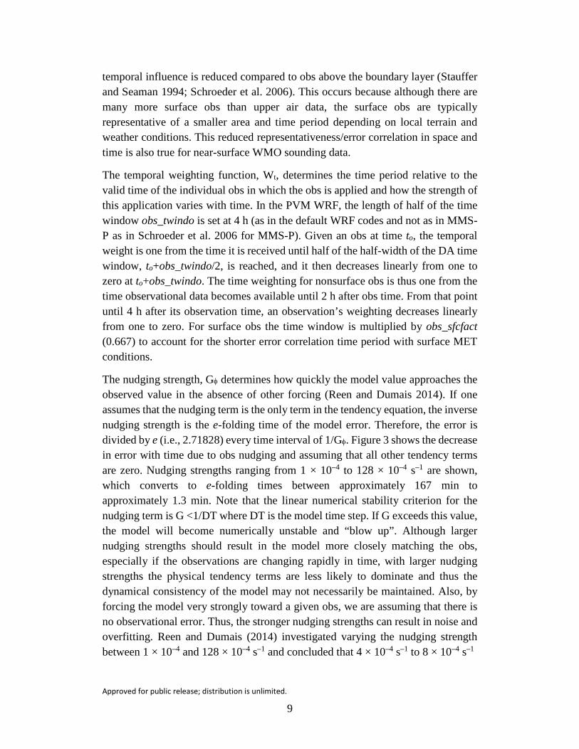
The nudging strength, Gφ determines how quickly the model value approaches the observed value in the absence of other forcing (Reen and Dumais 2014). If one assumes that the nudging term is the only term in the tendency equation, the inverse nudging strength is the e-folding time of the model error. Therefore, the error is divided by e (i.e., 2.71828) every time interval of 1/Gφ. Figure 3 shows the decrease in error with time due to obs nudging and assuming that all other tendency terms are zero. Nudging strengths ranging from 1 × 10–4 to 128 × 10–4 s–1 are shown, which converts to e-folding times between approximately 167 min to approximately 1.3 min. Note that the linear numerical stability criterion for the nudging term is G <1/DT where DT is the model time step. If G exceeds this value, the model will become numerically unstable and “blow up”. Although larger nudging strengths should result in the model more closely matching the obs, especially if the observations are changing rapidly in time, with larger nudging strengths the physical tendency terms are less likely to dominate and thus the dynamical consistency of the model may not necessarily be maintained. Also, by forcing the model very strongly toward a given obs, we are assuming that there is no observational error. Thus, the stronger nudging strengths can result in noise and overfitting. Reen and Dumais (2014) investigated varying the nudging strength between 1 × 10–4 and 128 × 10–4 s–1 and concluded that 4 × 10–4 s–1 to 8 × 10–4 s–1


10

seemed to work best. The nudging coefficient, Gφ, was set to 4 × 10–4 s–1 as in Stauffer and Seaman (1994) and subsequent Penn State published applications for all 3 predictive model variables in this study.

Fig. 3 Decrease of model error with time when nudging with various nudging weights and assuming that all of the physical tendency terms are zero

Setting the nudging coefficient at 4 × 10–4/s will reduce the difference between the modeled grid value and the obs by greater than 90% in 2 h if all physical forcings are zero. The value of G represents a compromise between too small a number, which leads to smaller reductions in the differences, and larger G, which will more rapidly reduce the differences but at the possible cost of inducing spurious effects on the forecast.

In the results that appear in this report, there are several WMO obs sites that fall within the outer 3,600 × 3,600 km domain (Domain 1, 36-km grid spacing). That domain defines the lateral boundaries of the middle 12-km domain (Domain 2) in which fewer WMO sites lie. It in turn defines the lateral boundary condition of the finest 4-km domain (Domain 3). For the results here, the center point was set to the MET station at YPG. The 1200 UTC YPG sounding from that site usually is included in WMO disseminated reports received by the PVM and so it was used directly in predictions on all domains. No other WMO site falls within Domain 3, so the DA impacts in Domain 3 are from the direct impact of the current YPG sounding, or indirect impact of previously assimilated YPG soundings, and any surface obs and indirect impacts from the propagation of corrections through its


11

lateral boundaries from assimilation of WMO soundings and surface obs on Domains 1 and 2.

2 Methodology and Test Procedures

2.1 Testing Profiler DA

The PVM was set up to assimilate WMO soundings (including the YPG MET station) and surface data from when received and processed until the data “aged out”. Typically, for free atmosphere obs in these artillery meteorology systems, “aged out” means that the data are 4 or more hours old. Surface data age out more quickly so that their weighting declines to zero by 2 2/3 h after obs time. To test the DA, there were 2 MILTOPES (MILTOPE refers to ruggedized laptops used by the military), and both had the latest version of PVM software installed. One PVM system was set up to receive timely WMO and surface data from a special folder set up at the 557th WW while the other PVM received no WMO and surface data.

2.2 Limitations to the Testing

In order to test the PVM’s DA, validation data were required. A major problem in testing this system’s DA is that there are limitations in using the WMO sounding network for validation. WMO soundings are typically made every 12 h; however, the effect of assimilating soundings made 12 h earlier largely or completely disappears by the time of the validating soundings. To get around this limitation, we tried testing the systems for locations in central Germany where there are several observing sites at which soundings are made 4 times daily spaced 6 h apart in time (0600, 1200, 1800, and 0000 UTC). The central German soundings while offering a better validation were still limited because their validation observation time is still 2 h after the DA time window that is 4 h after obs time, and so some or much of the effect of DA could be lost in the interim.

Another alternative considered is the European Wind Profiling Radar network. This network includes 30 sites extending mainly across western and central Europe. There is also one site quite far north located at Kiruna, Sweden. At many of the sites, the obs are made by 1,290-MHz radar; depending on the strength of radar backscatter energy, the maximum height for wind observations is about 6-km above ground level (AGL) but it is frequently lower. At a few sites, however, 482-MHz radar is used; with high mode these radars can measure winds to as high as 16-km AGL and usually can provide winds up to 14–15-km AGL. These wind profiler sites, however, do not observe temperature, pressure, and moisture except quite close to the ground where such data are observed using a Radar Acoustic Sounding


12

System (RASS). Therefore, because the profiler sites offer numerous wind obs but no temperature or pressure data above the surface, we continued looking for appropriate validation data sources.

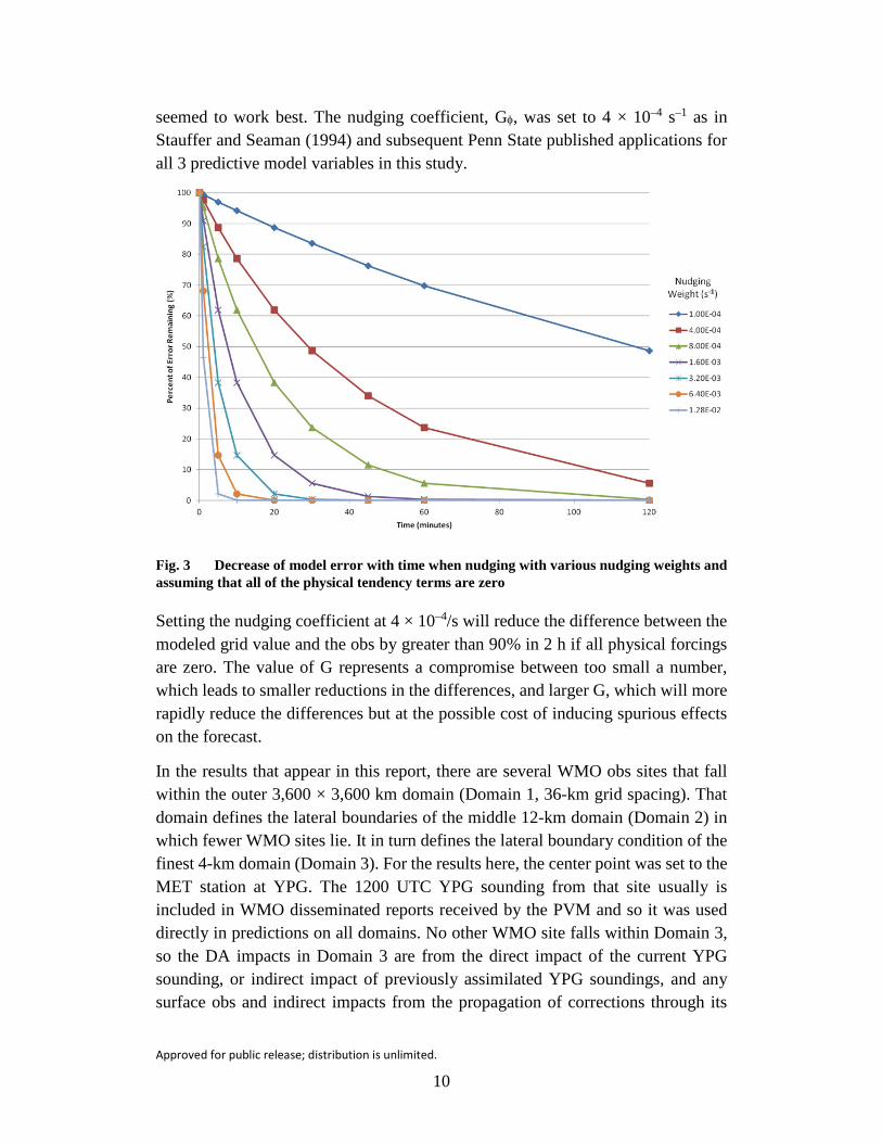
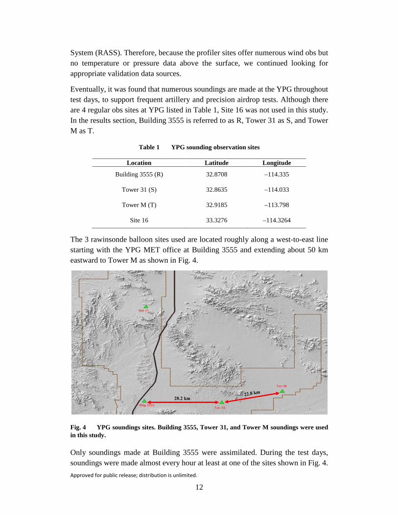
Eventually, it was found that numerous soundings are made at the YPG throughout test days, to support frequent artillery and precision airdrop tests. Although there are 4 regular obs sites at YPG listed in Table 1, Site 16 was not used in this study. In the results section, Building 3555 is referred to as R, Tower 31 as S, and Tower M as T.

Table 1 YPG sounding observation sites

Location Latitude Longitude

Building 3555 (R) 32.8708 –114.335

Tower 31 (S) 32.8635 –114.033

Tower M (T) 32.9185 –113.798

Site 16 33.3276 –114.3264

The 3 rawinsonde balloon sites used are located roughly along a west-to-east line starting with the YPG MET office at Building 3555 and extending about 50 km eastward to Tower M as shown in Fig. 4.

Fig. 4 YPG soundings sites. Building 3555, Tower 31, and Tower M soundings were used in this study.

Only soundings made at Building 3555 were assimilated. During the test days, soundings were made almost every hour at least at one of the sites shown in Fig. 4.


13

The YPG MET office provided the times and locations of their soundings in advance so that the PVM messages could be generated coincidentally in time and place with the YPG soundings. The YPG MET office also provided a number of such soundings in their “redimet” format. The redimet format was readily converted into METCM format using a program developed by Cogan (2015).

The Building 3555 sounding site is included on the WMO station list (74004, 1Y7) and it is usually disseminated for all 3-hourly launch times and included with the other world-wide WMO soundings. Soundings at the other YPG stations are not included in the WMO data dissemination. After this test it was discovered that the Building 3555 sounding was received by the PVM not only at 1200 UTC but also at 1500, 1800, and 2100 UTC, if available. Although this complicates the analysis of this test’s data, it allows analysis of PVM accuracy by previous DA at the time of the Building 3555 sounding (since it would not yet have been assimilated), as well as a measure of the “fit to the data” in the hours after the sounding time at Building 3555 (74004). The other 2 soundings are always independent data for verification.

The PVM was set up so that its modeling domain was centered on Building 3555 and messages were generated at the 3 sites: Building 3555, Tower 31, and Tower M (also as above). However, the system assimilated the Building 3555 sounding at the WMO table location as mentioned above or at a point 70.81 km south-southeast of where it should have been located. The US Army Research Laboratory (ARL) is working with the PVM contractor to get the table corrected for the YPG location. In the course of investigating this, it was discovered that there are other WMO site locations that are also incorrectly located on the WMO table; the locations of these other sites will also be corrected. Please note that the locations at which the PVM messages were generated and the sites at which the verification soundings were taken are correct.

2.3 Soundings Test Procedure

1) Synchronize laptop times. This was important and necessary so that the initializations on all laptops were the same or at least very nearly the same (to within 10–20 s).

2) Set center point location in the PVM’s graphical user interface (GUI) to location of YPG Building 3555.

3) Download 1200 UTC GFS data (North America) from website.

4) Read GFS data on all laptops.


14

5) Follow start procedure for PVM laptop (Step 6).

6) PVM:

a. Initially the data receipt switch was set to OFF.

b. Start PVM just after 2052 or 2152 UTC. This allowed the systems to complete 4 or even 6 modeling cycles (30 min each cycle) before METCMs for 0000 UTC were generated on both systems. It also allowed the messages to be generated at precisely 0000 UTC. Four modeling cycles were deemed a sufficiently long forecast time to expose any initialization differences between the test systems when the comparison messages were generated, but 6 modeling cycles were done if feasible.

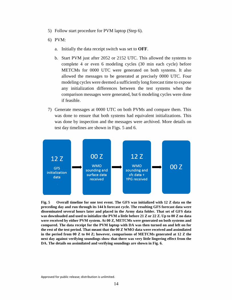
7) Generate messages at 0000 UTC on both PVMs and compare them. This was done to ensure that both systems had equivalent initializations. This was done by inspection and the messages were archived. More details on test day timelines are shown in Figs. 5 and 6.

Fig. 5 Overall timeline for one test event. The GFS was initialized with 12 Z data on the preceding day and run through its 144 h forecast cycle. The resulting GFS forecast data were disseminated several hours later and placed in the Army data folder. That set of GFS data was downloaded and used to initialize the PVM a little before 21 Z or 22 Z. Up to 00 Z no data were received by either PVM system. At 00 Z, METCMs were generated on both systems and compared. The data receipt for the PVM laptop with DA was then turned on and left on for the rest of the test period. That meant that the 00 Z WMO data were received and assimilated in the period from 00 Z to 04 Z; however, comparisons of METCMs generated at 12 Z the next day against verifying soundings show that there was very little lingering effect from the DA. The details on assimilated and verifying soundings are shown in Fig. 6.


15

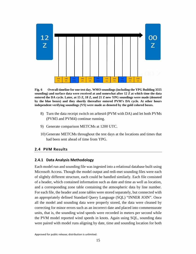
Fig. 6 Overall timeline for one test day. WMO soundings (including the YPG Building 3555 sounding) and surface data were received at and somewhat after 12 Z at which time the data entered the DA cycle. Later, at 15 Z, 18 Z, and 21 Z new YPG soundings were made (denoted by the blue boxes) and they shortly thereafter entered PVM’s DA cycle. At other hours independent verifying soundings (VS) were made as denoted by the gold colored boxes.

8) Turn the data receipt switch on arltest4 (PVM with DA) and let both PVMs (PVM3 and PVM4) continue running.

9) Generate comparison METCMs at 1200 UTC.

10) Generate METCMs throughout the test days at the locations and times that had been sent ahead of time from YPG.

2.4 PVM Results

2.4.1 Data Analysis Methodology

Each model run and sounding file was ingested into a relational database built using Microsoft Access. Though the model output and redi-met sounding files were each of slightly different structure, each could be handled similarly. Each file consisted of a header, which contained information such as date and time as well as location, and a corresponding zone table containing the atmospheric data by line number. For each file, the header and zone tables were stored separately, but connected with an appropriately defined Standard Query Language (SQL) “INNER JOIN”. Once all the model and sounding data were properly stored, the data were cleaned by correcting for minor errors such as an incorrect date and placed into commensurate units, that is, the sounding wind speeds were recorded in meters per second while the PVM model reported wind speeds in knots. Again using SQL, sounding data were paired with model runs aligning by date, time and sounding location for both


16

the “With” and “Without DA” cases to produce the sample comparison points in Table 2.

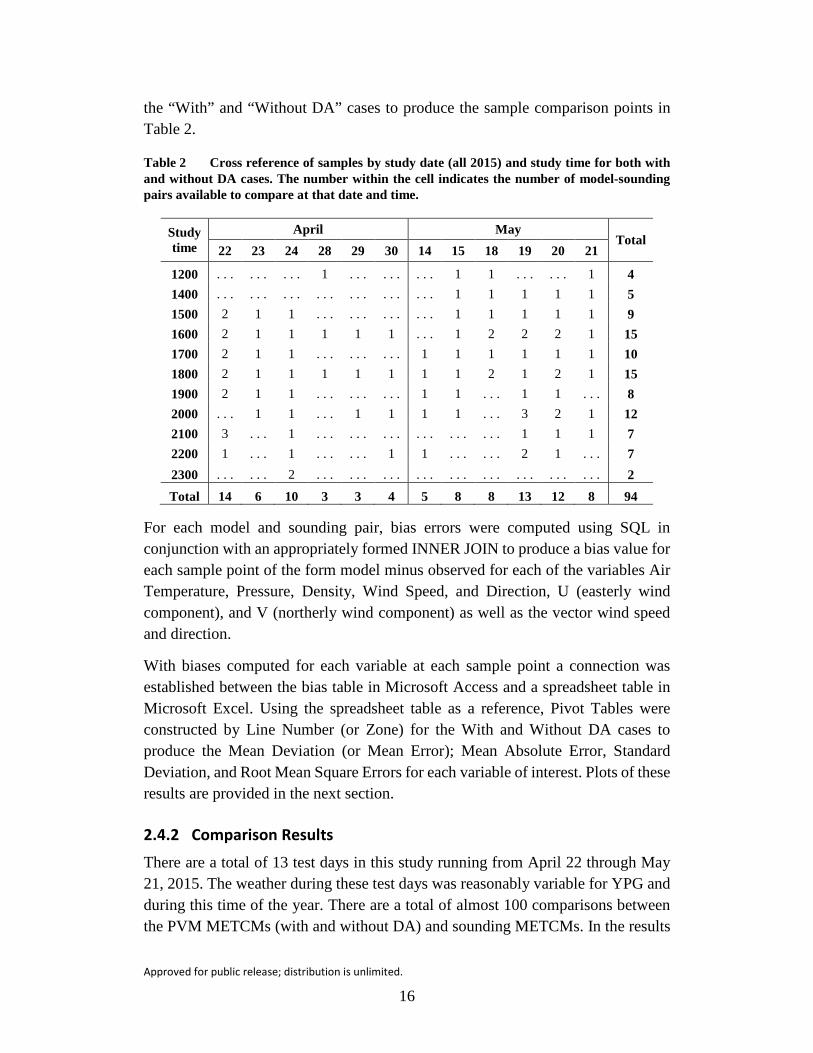
Table 2 Cross reference of samples by study date (all 2015) and study time for both with and without DA cases. The number within the cell indicates the number of model-sounding pairs available to compare at that date and time.

Study time

April May Total

22 23 24 28 29 30 14 15 18 19 20 21

1200 . . . . . . . . . 1 . . . . . . . . . 1 1 . . . . . . 1 4 1400 . . . . . . . . . . . . . . . . . . . . . 1 1 1 1 1 5 1500 2 1 1 . . . . . . . . . . . . 1 1 1 1 1 9 1600 2 1 1 1 1 1 . . . 1 2 2 2 1 15 1700 2 1 1 . . . . . . . . . 1 1 1 1 1 1 10 1800 2 1 1 1 1 1 1 1 2 1 2 1 15 1900 2 1 1 . . . . . . . . . 1 1 . . . 1 1 . . . 8 2000 . . . 1 1 . . . 1 1 1 1 . . . 3 2 1 12 2100 3 . . . 1 . . . . . . . . . . . . . . . . . . 1 1 1 7 2200 1 . . . 1 . . . . . . 1 1 . . . . . . 2 1 . . . 7 2300 . . . . . . 2 . . . . . . . . . . . . . . . . . . . . . . . . . . . 2 Total 14 6 10 3 3 4 5 8 8 13 12 8 94

For each model and sounding pair, bias errors were computed using SQL in conjunction with an appropriately formed INNER JOIN to produce a bias value for each sample point of the form model minus observed for each of the variables Air Temperature, Pressure, Density, Wind Speed, and Direction, U (easterly wind component), and V (northerly wind component) as well as the vector wind speed and direction.

With biases computed for each variable at each sample point a connection was established between the bias table in Microsoft Access and a spreadsheet table in Microsoft Excel. Using the spreadsheet table as a reference, Pivot Tables were constructed by Line Number (or Zone) for the With and Without DA cases to produce the Mean Deviation (or Mean Error); Mean Absolute Error, Standard Deviation, and Root Mean Square Errors for each variable of interest. Plots of these results are provided in the next section.

2.4.2 Comparison Results

There are a total of 13 test days in this study running from April 22 through May 21, 2015. The weather during these test days was reasonably variable for YPG and during this time of the year. There are a total of almost 100 comparisons between the PVM METCMs (with and without DA) and sounding METCMs. In the results


17

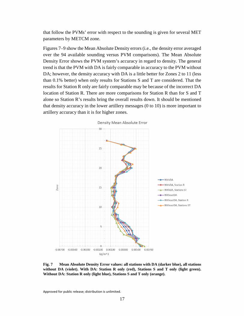
that follow the PVMs’ error with respect to the sounding is given for several MET parameters by METCM zone.

Figures 7–9 show the Mean Absolute Density errors (i.e., the density error averaged over the 94 available sounding versus PVM comparisons). The Mean Absolute Density Error shows the PVM system’s accuracy in regard to density. The general trend is that the PVM with DA is fairly comparable in accuracy to the PVM without DA; however, the density accuracy with DA is a little better for Zones 2 to 11 (less than 0.1% better) when only results for Stations S and T are considered. That the results for Station R only are fairly comparable may be because of the incorrect DA location of Station R. There are more comparisons for Station R than for S and T alone so Station R’s results bring the overall results down. It should be mentioned that density accuracy in the lower artillery messages (0 to 10) is more important to artillery accuracy than it is for higher zones.

Fig. 7 Mean Absolute Density Error values: all stations with DA (darker blue), all stations without DA (violet). With DA: Station R only (red), Stations S and T only (light green). Without DA: Station R only (light blue), Stations S and T only (orange).


18

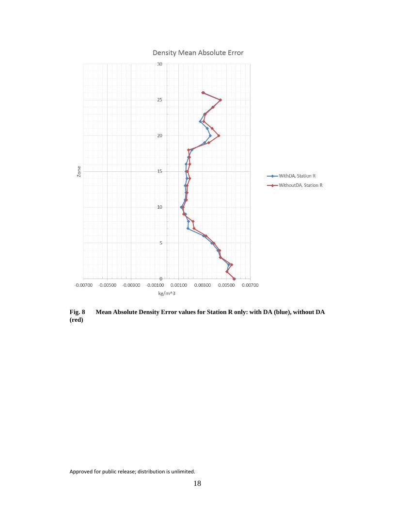
Fig. 8 Mean Absolute Density Error values for Station R only: with DA (blue), without DA (red)


19

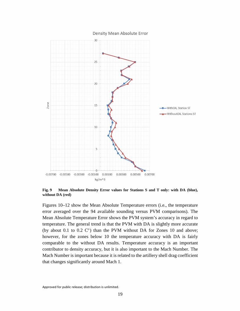
Fig. 9 Mean Absolute Density Error values for Stations S and T only: with DA (blue), without DA (red)

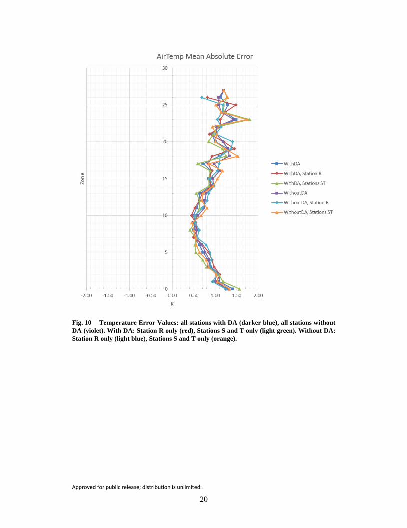
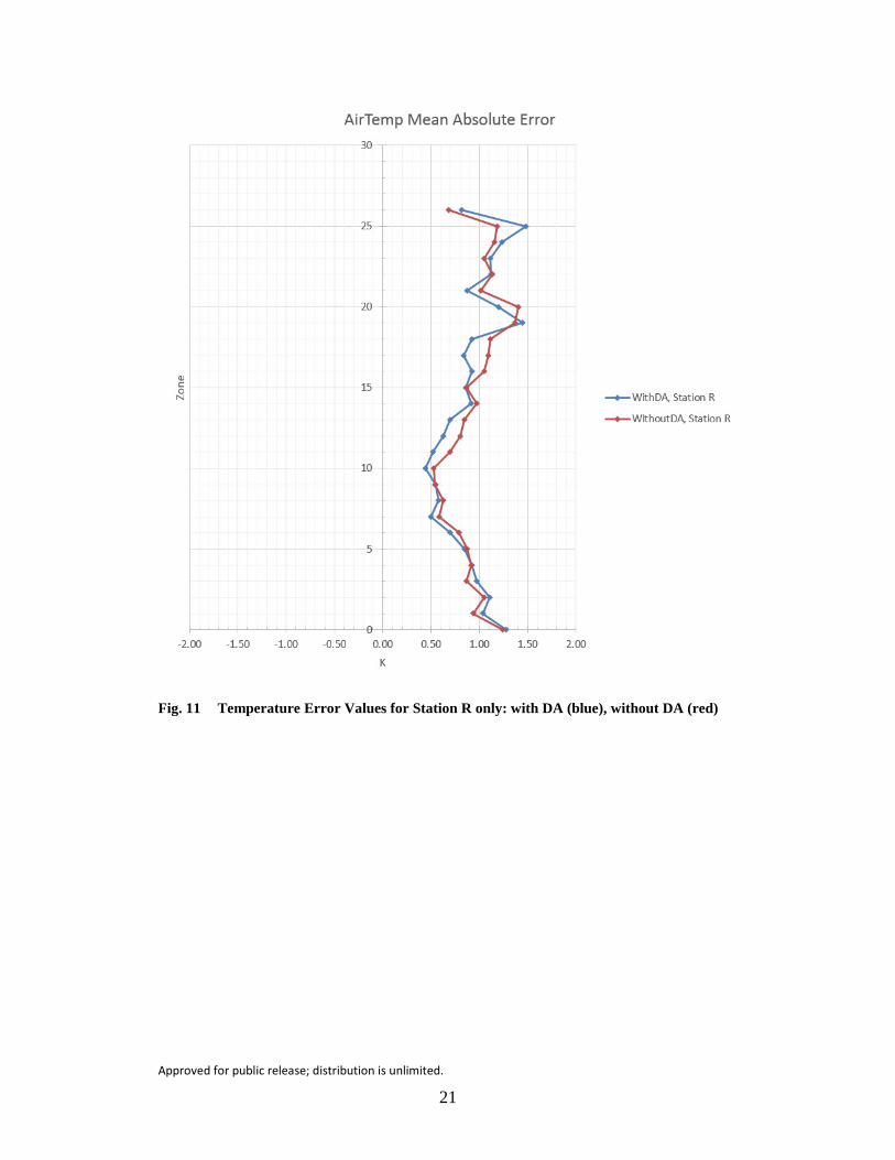
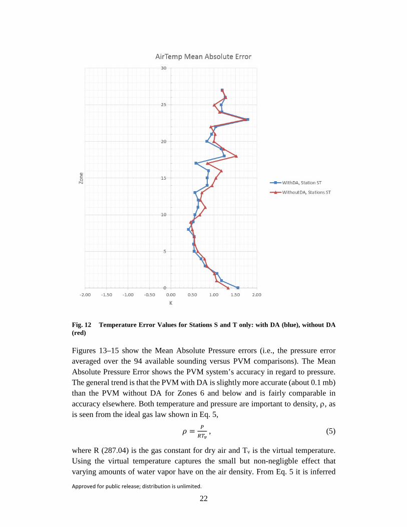
Figures 10–12 show the Mean Absolute Temperature errors (i.e., the temperature error averaged over the 94 available sounding versus PVM comparisons). The Mean Absolute Temperature Error shows the PVM system’s accuracy in regard to temperature. The general trend is that the PVM with DA is slightly more accurate (by about 0.1 to 0.2 C°) than the PVM without DA for Zones 10 and above; however, for the zones below 10 the temperature accuracy with DA is fairly comparable to the without DA results. Temperature accuracy is an important contributor to density accuracy, but it is also important to the Mach Number. The Mach Number is important because it is related to the artillery shell drag coefficient that changes significantly around Mach 1.


20

Fig. 10 Temperature Error Values: all stations with DA (darker blue), all stations without DA (violet). With DA: Station R only (red), Stations S and T only (light green). Without DA: Station R only (light blue), Stations S and T only (orange).


21

Fig. 11 Temperature Error Values for Station R only: with DA (blue), without DA (red)


22

Fig. 12 Temperature Error Values for Stations S and T only: with DA (blue), without DA (red)

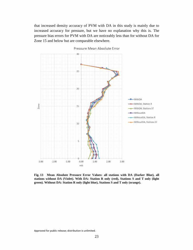
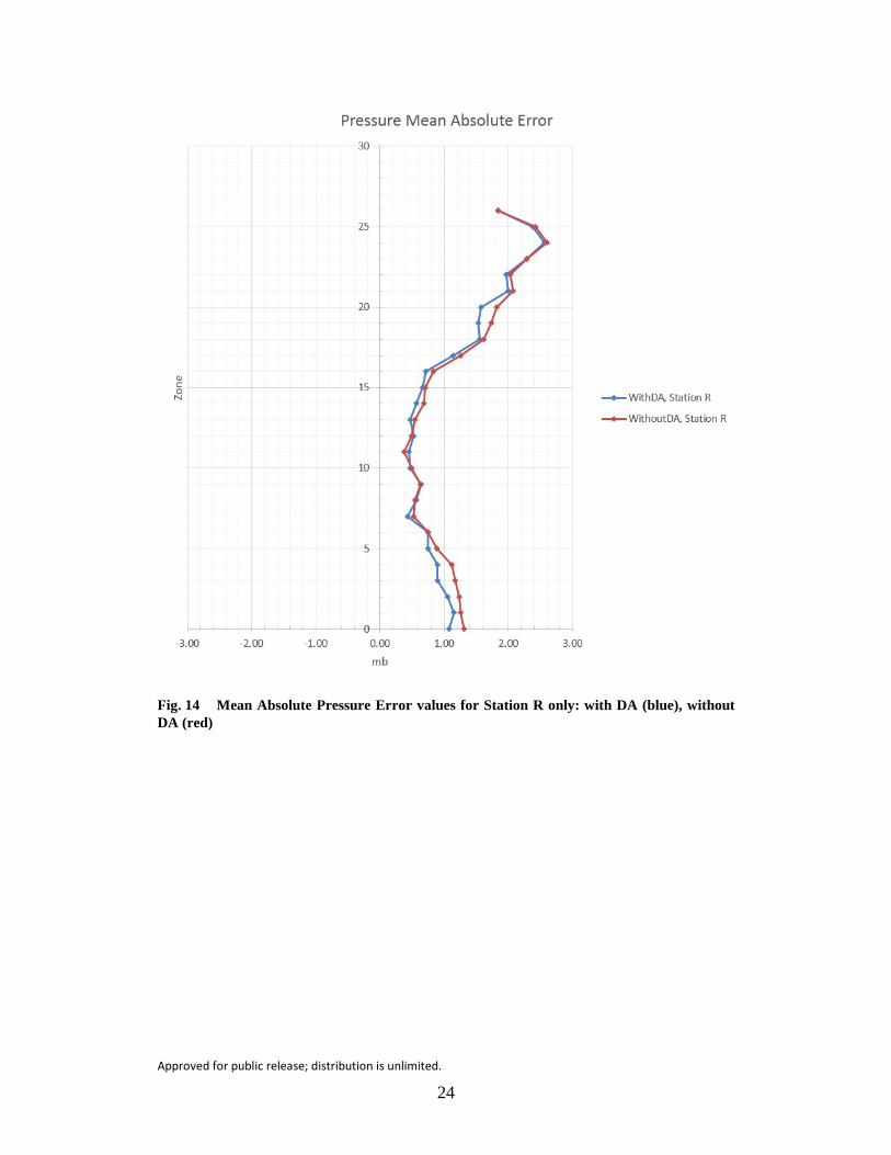
Figures 13–15 show the Mean Absolute Pressure errors (i.e., the pressure error averaged over the 94 available sounding versus PVM comparisons). The Mean Absolute Pressure Error shows the PVM system’s accuracy in regard to pressure. The general trend is that the PVM with DA is slightly more accurate (about 0.1 mb) than the PVM without DA for Zones 6 and below and is fairly comparable in accuracy elsewhere. Both temperature and pressure are important to density, ρ, as is seen from the ideal gas law shown in Eq. 5,

𝜌𝜌 = 𝑃𝑃𝑅𝑅𝑇𝑇𝑣𝑣

, (5)

where R (287.04) is the gas constant for dry air and Tv is the virtual temperature. Using the virtual temperature captures the small but non-negligble effect that varying amounts of water vapor have on the air density. From Eq. 5 it is inferred


23

that increased density accuracy of PVM with DA in this study is mainly due to increased accuracy for pressure, but we have no explanation why this is. The pressure bias errors for PVM with DA are noticeably less than for without DA for Zone 15 and below but are comparable elsewhere.

Fig. 13 Mean Absolute Pressure Error Values: all stations with DA (Darker Blue), all stations without DA (Violet). With DA: Station R only (red), Stations S and T only (light green). Without DA: Station R only (light blue), Stations S and T only (orange).


24

Fig. 14 Mean Absolute Pressure Error values for Station R only: with DA (blue), without DA (red)


25

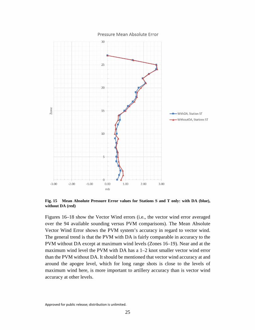
Fig. 15 Mean Absolute Pressure Error values for Stations S and T only: with DA (blue), without DA (red)

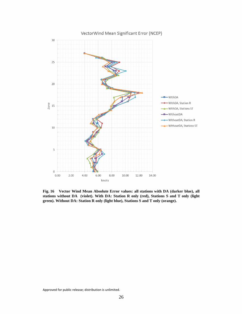
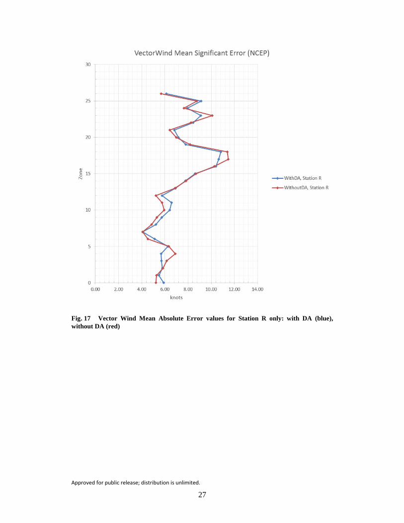
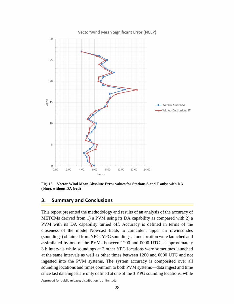
Figures 16–18 show the Vector Wind errors (i.e., the vector wind error averaged over the 94 available sounding versus PVM comparisons). The Mean Absolute Vector Wind Error shows the PVM system’s accuracy in regard to vector wind. The general trend is that the PVM with DA is fairly comparable in accuracy to the PVM without DA except at maximum wind levels (Zones 16–19). Near and at the maximum wind level the PVM with DA has a 1–2 knot smaller vector wind error than the PVM without DA. It should be mentioned that vector wind accuracy at and around the apogee level, which for long range shots is close to the levels of maximum wind here, is more important to artillery accuracy than is vector wind accuracy at other levels.


26

Fig. 16 Vector Wind Mean Absolute Error values: all stations with DA (darker blue), all stations without DA (violet). With DA: Station R only (red), Stations S and T only (light green). Without DA: Station R only (light blue), Stations S and T only (orange).


27

Fig. 17 Vector Wind Mean Absolute Error values for Station R only: with DA (blue), without DA (red)


28

Fig. 18 Vector Wind Mean Absolute Error values for Stations S and T only: with DA (blue), without DA (red)

3. Summary and Conclusions

This report presented the methodology and results of an analysis of the accuracy of METCMs derived from 1) a PVM using its DA capability as compared with 2) a PVM with its DA capability turned off. Accuracy is defined in terms of the closeness of the model Nowcast fields to coincident upper air rawinsondes (soundings) obtained from YPG. YPG soundings at one location were launched and assimilated by one of the PVMs between 1200 and 0000 UTC at approximately 3 h intervals while soundings at 2 other YPG locations were sometimes launched at the same intervals as well as other times between 1200 and 0000 UTC and not ingested into the PVM systems. The system accuracy is composited over all sounding locations and times common to both PVM systems—data ingest and time since last data ingest are only defined at one of the 3 YPG sounding locations, while


29

verification is completely independent at the other 2 sounding locations for all verification times.

The PVM’s Nowcasting accuracy was compared to the currently fielded artillery MET system, the CMD-P in an earlier report by Cogan et al. (2014). That report showed that the PVM had nearly the same or slightly better accuracy than the CMD-P as related to coincident rawinsonde (sounding) data, but the comparisons were based on testing in which both systems relied only on GFS data for initialization and did not include assimilation of WMO data as was done for the results reported here.

Two PVM systems were used. The first system was used as in Cogan et al. (2014), that is, no WMO data were received and used in producing the Nowcast/forecast results and the METCMs shown in that report. The second system, had direct network connections to a special data folder at the 557th WW, was able to move newly received WMO data from that folder to the test system every 6 min during the testing. The WMO data are typically available every hour at the surface and every 12 h above the surface. The additional YPG rawinsondes used for assimilation in this test were generally available every 3 h between 1200 and 0000 UTC. The comparisons were made in terms of the accuracy of the common MET variables of wind, pressure and temperature, and also in terms of the variables most pertinent to artillery accuracy, air density, and vector wind error.

Both systems were initialized and started simultaneously with the same data and run to create a baseline comparison without DA in which METCMs were generated on both systems and immediately compared in order to verify that they had identical or nearly identical initializations. Subsequently, receipt of data was turned on for the DA system and the 2 systems continued with their respective 30-min Nowcast cycles throughout the rest of the test period.

Each model run and sounding file was ingested into a relational database built using Microsoft Access. Once all the model and sounding data were properly stored, the data were quality-controlled by correcting for minor errors such as an incorrect date and placed into commensurate units, that is, the sounding wind speeds were recorded in meters per second while the PVM model reported wind speeds in knots. Using SQL, sounding data were paired with model runs aligning by date, time, and sounding location for both the “With” and “Without DA” cases to produce the sample comparison points

There are a total of 13 test days in this study running from April 22 through May 21, 2015. The weather during these test days was reasonably variable for YPG and


30

at that time of the year. Altogether, there are a total of almost 100 comparisons between the PVM METCMs (with and without DA) and sounding METCMs.

There were 3 YPG sites at which soundings were made: Building 3555, Tower 31, and Tower M. Only soundings made at Building 3555 were assimilated, but it was discovered after the conclusion of this test, that Building 3555’s location is incorrect in the WMO table of station locations. The WMO location is used in the system to place an obs so the difference between an observed value and the model forecast is calculated and applied at and around the WMO location point. Because of the incorrect position there was an error in the difference and the amount of this error was increased because it was applied to a somewhat different location than it should have been.

The DA is fairly comparable in density accuracy to the PVM without DA; however, the density accuracy with DA is a little better for Zones 2 to 11 (less than 0.1% better) when only the results for Stations S and T are considered. That the results for Station R only are fairly comparable may be because of the incorrect DA location of Station R. Density accuracy in the lower artillery message Zones (0 to 10) is more important to artillery accuracy than it is for higher zones.

The PVM with DA is slightly more than accurate (by about 0.1 to 0.2 C°) than the PVM without DA for Zones 10 and above; however, for zones below 10 the temperature accuracy with DA is fairly comparable to without DA results. Temperature accuracy is important for Mach Number.

The PVM with DA is slightly more than accurate in pressure (about 0.1 mb) than the PVM without DA for Zones 6 and below, and is fairly comparable in accuracy elsewhere. While, both temperature and pressure are important to density, it may be inferred that the slightly increased density accuracy of PVM with DA in this study is mainly due to its increased accuracy for pressure, but we have no explanation why this is.

The PVM with DA is fairly comparable in accuracy to the PVM without DA for the vector wind except at maximum wind levels (Zones 16–19). Near and at the maximum wind level the PVM with DA has a 1–2 knot smaller vector wind error than the PVM without DA. Vector wind accuracy at and around the level of maximum wind is somewhat more important to artillery accuracy than is vector wind accuracy at other levels.

Overall, the PVM with DA is slightly more accurate than the PVM without DA, but firing simulations with the General Trajectory model should be done to see if these differences lead to additional artillery accuracy. In most cases, the difference between an obs and a forecast field that is 71-km distant, will be greater than the


31

difference between the obs and the forecast field at the obs point. Therefore, the incorrect WMO station location used in the DA of this study degrades the value of the DA. In addition, this difference was applied at the wrong position, further degrading the DA. That is why we believe that there may be further advantage to using DA in PVM, than was shown in this study, but that will have to be shown in future studies using a corrected WMO station table.


32

4. References and Notes

Bei N, de Foy B, Lei W, Zaval M, Molina LT. Using 3DVAR data assimilation system to improve ozone simulations in the Mexico City basin. Atmos. Chem. Phys. 2008;8: 7353–7366. doi:10.5194/acp-8-7353-2008.

Cogan J. A generalized method for vertical profiles of mean layer values of meteorological variables. Adelphi Laboratory Center (MD): Army Research Laboratory (US); 2015 Sep. Report No.: ARL-TR-7434.

Cogan J, Haines P., Seik J, and Wetmore A. Accuracy of Computer Meteorological Messages (METCMs) from profiler virtual module vs. from computer, meteorological data-profiler. Adelphi Laboratory Center (MD): Army Research Laboratory (US); 2014 Dec. Report No.: ARL-TR-7149.

Fujita T, Stensrud DJ, Dowell DC. Surface data assimilation using an ensemble Kalman filter approach with initial condition and model physics uncertainty. Mon. Wea. Rev. 2007;135:1846–1868.

Kalnay E. Atmospheric modeling, data assimilation and predictability. Cambridge (MA): Cambridge University Press: 2003.

Lei L, Stauffer DR, Deng A. A hybrid nudging-ensemble Kalman filter approach to data assimilation in WRF/DART. Q.J.R Meterorol. Soc. 2012:DOI:10.1002/qj.1939.

Liu C, Xiao Q, Wang B. An ensemble-based four-dimensional variational data assimilation scheme. part 1: Technical formulation and preliminary test. Mon. Weather Rev. 2008;136:3363–3373:DOI:10.1175/2008MWR2312.1.

Reen BP. A brief guide to observation nudging in WRF. Adelphi (MD): Unpublished manuscript; 2015.

Reen BP, Dumais RE. Assimilating tropospheric airborne meteorological data reporting (TAMDAR) observations and the relative value of other observation types. Adelphi Laboratory Center (MD): Army Research Laboratory (US); 2014 Aug. Report No.: ARL-TR-7022.

Reen BP, Stauffer DR. Data Assimilation Strategies in the Planetary Boundary Layer. Bound-Lay Meteor. 2010;137:237–269.

Rogers RE, Deng A, Stauffer DR, Gaudet BJ, Jia Y, Soong S, Tanrikulu S. Application of the Weather Research and Forecasting Model for Air Quality Modeling in the San Francisco Bay Area. J. Appl Meteor and Climatol. 2013;52:1953–1973.


33

Schroeder AJ, Stauffer DR, Seaman NL, Deng A, Gibbs AM, Hunter GK, Young GS. An Automated high-resolution, rapidly relocatable meteorological nowcasting and prediction system. Mon. Wea. Rev. 2006;134:1228–1256.

Stauffer DR, Seaman SL. Multiscale four-dimensional data assimilation. J. Appl. Meteor. 1994;33:416–434.

Stauffer DR, Deng A, Hunter GK, Gibbs AM, Zielonka JR, Tinklepaugh K, Dobek J. NWP goes to war . . . , Preprints. Paper presented at: 22nd Conference on Weather Analysis and Forecasting/18th Conference on Numerical Weather Prediction; 2007 June 25–29; Park City (UT). 2007a.

Stauffer DR, Hunter GK, Deng A, Zielonka JR, Tinklepaugh K, Hayes P, Kiley C. On the role of atmospheric data assimilation and model resolution on model forecast accuracy for the Torino Winter Olympics, Preprints. Paper presented at: 22nd Conference on Weather Analysis and Forecasting/18th Conference on Numerical Weather Prediction; 2007 June 25–29; Park City (UT). 2007b.

Warner T. Numerical weather and climate prediction. Cambridge (UK): Cambridge University Press: 2011: ISBN: 978-0-521-51389-0.

Zhang F, Zhang M, Poterjoy J. E3DVar: Coupling an ensemble Kalman filter with three-dimensional variational data assimilation in a limited-area weather prediction model and comparison to E4DVar. Mon. Wea. Rev. 2013;141:900–917.


34



35

Appendix A. Required Additional Miltope Configuration and Scripts

This appendix appears in its original form, without editorial change.


36

Four military field hard laptops (Miltopes) were used to test the Profiler Virtual Module (PVM) and the Computer, Meteorological Data-Profiler (CMD-P). Two were installed with RHEL 5 and two with RHEL 6. We had to establish that these systems had the proper Certificate of Networthiness (CoN) before allowing them on our network without all the management/scanning software our systems require. CoNs were provided for CMD-P and PVM and for the RHEL 5 Operating System. Oddly, we were informed that RHEL 6 did not have a CoN because "it did not need it". Fortunately, our IAM permitted this. Because the Miltopes are secured field units, their operating systems, RHEL 5 and 6, required "opening", much as the hood of a car is opened, in the following ways, to allow us to perform the requisite testing: An existing script, IPchg, was greatly enhanced to accomplish the following configurations:

Configure/Unconfigure the Network Interface Card (NIC) to connect to the ARL network. PVM has a required section to set up the NIC; however, the gateway was never set up properly by PVM, and the Miltopes would lose network connectivity. IPchg was run after PVM to restore network connectivity.

When IPchg attempted changing the IP and set of the gateway,

NetworkManager would intrude with unworkable values. nm-connection-editor would show values that were not in the NIC configuration files (/etc/sysconfig/network and /etc/sysconfig/network-script/ifcfg-eth0). IPchg does a /etc/init.d/NetworkManager stop to shut it down and uses chkconfig to prevent it from restarting at boot.

IPchg creates a /etc/resolv.conf for the ARL DNS server so network

connection by hostname can be achieved.

Because the Miltopes have a very stiff keyboards, the monitors are small, and the systems use hard to see gnome default terminal settings, a normal ARL RHEL 6 system was used to develop the scripts documented here. Connection to the ARL workstation and between each of the Miltopes was configured by IPchg by adding these hosts to /etc/hosts.allow (TCP wrapper config)

For connection to the ARL development workstation and to AFWA, the ssh deamon (sshd) had to be turned on so that it would be restart after a reboot. IPchg accomplished this. However, the sshd start up script on the RHEL5 systems (/etc/init.d/sshd), had a bug which attempted to generate an rsa1 key when the sshd_config


37

was configured for Protocol 2. This line was commented out by IPchg before it started sshd.

In order to automatically download data from AFWA without having to enter

a password every 3 minutes, public and private keys were require. IPchg backs up1 /etc/ssh/ssh_config, then modifies it so "KerberosAuthentication no" is commented out.

The Miltopes also configure the OS firewall to block ssh, upon which rsync

depends. After backing up /etc/sysconfig/iptables, IPchg modifies it to allow ssh and sftp, flush the firewall, then restarts it:

# IPT=/etc/sysconfig/iptables # iptables -F; iptables-restore < $IPT # service iptables save

selinux constantly annoys with GUI popups which we do not have the

capacity to service; therefore, IPchg comments out the "SELINUX=permissive" setting and inserts the "SELINUX=disabled" setting into /etc/selinux/config.

The kernel audit feature is not configure properly and overruns the

/var/log/messages with error messages. IPchg removes this option from /boot/grub/grub.conf after backing up grub.conf

We frequently needed to login to another terminal as root to make adjustment

(like restarting the network after PVM had miss configured it). /etc/securetty prevented this so IPchg adds a full list of pseudo and hard terminals to this file.

Configure ntp for ARL time servers with ntp keys

A new script, dnldr, was written to download data from AFWA using rsync when run without options. By logging when new data has been added to the AFWA site (via rsync), the script verified when pulled data had been processed. If it has not been processed, new data is copied to the PVM consumption directory. This ensures data is fed into PVM only once. The download will only occur if a START file exists in the test users home directory which is used control when to start feeding PVM data files. dnldr's options are as follows: The -s Option

Schedules rsync, from within dnldr, to run every 3 minutes using crontab. rsync output was redirected by crontab to a log file used ensure all data processed and that it is only processed once.

1 The "back up" convention is to save the file as a hidden file with a .org extension. For example, /etc/ssh/ssh_config would be backed up as /etc/ssh/.ssh_config.org.


38

-s adds the test user to the profiler group, so the user can write AFWA data to the PVM consumption directory, and the wheel group so the test user can sudo to root for debugging and maintenance chores.

-s sets permissions for the profiler group so members can write to PVM data consumption directory (RHEL5:/h/data/IncomingData/Tvsat, and RHEL6:/h/data/incoming)

-s setsup/tearsdown entries in /etc/sudoers to allow the test user to reset system time, and switch to root user as necessary.

The -u Option Undo everything -s has setup

The -p Option rsync determines what files to download based on the files already

downloaded. -p "primes the pump" by pre-downloading all AFWA files. When PVM starts, it then will be fed only next new AFWA file from that point forward.

The -c Option

Over time the AFWA site discards older data files. If dnldr has been run previous it will maintain those older file. -c should be run before -p to clean out all AFWA files. -p should then be used to collect only current AFWA files.

The -t Option

Allows the test user to set the hardware and operating system clock. (This was quicker that trying get ntp working with the restriction set on the Miltopes and in the ARL network.)

The -h Option

Show a help screen describing the same options described in this section.

Running KEYINSTL -r (a previous existing script) in the AFWA user account sets up the ssh public key in ~/.ssh/authorized_keys. Running KEYINSTL without options on the Miltope in the test user's account created the matching private key in ~/.ssh/id_dsa. Assuming "PubkeyAuthentication yes" and "AuthorizedKeysFile .ssh/authorized_keys" sshd_config settings are in force on the remote AFWA system, allows the dnldr script to perform its rsync without the need for a password. A previously existing gconf script, gc, was modified to add an AFWA icon to the top task bar. When PVM is ready to run, clicking this icon runs the ~/.config/AFWAstart script which in turn creates the ~/START file. dnldr


39

verifies ~/START's existence before it will run rsync. Clicking the AFWA icon upon completion of PVM testing causes AFWAstart to remove ~/START. Thus stops dnldr from rsync'ing data from AFWA. gnome-terminal, logout, and shutdown icons were added as well.

The modified install.dots script extracts, from an embedded tarball, .bashrc, .profile, .vimrc, and .Xdefaults. .bashrc contains configuration to

Set the terminal prompt to show hostname and absolute path to the current directory Set ls to show colors for file types Set an s alias which allows the test user to track the progress of an AFWA

data file from download directory through consumption directory along with the relevant log files.

.Xdefaults configures xterm to display in a reasonable fashion used locally on the Miltope or remotely from the ARL development system. install.dots also discovers what vim is available on the Miltope and configures .bashrc and .vimrc with convenient features for vi/vim according to the version installed. The tarPARSE script was created to manually examine AFWA data. Initially, all the downloaded tarballs are presented in a numbered paged menu. Upon selection, the specified tarball is extracted and the resulting files are presented as a second paged menu. Selection of a file at displays its content. Exit from viewing returns to the menu of extracted files. At this point, the previously viewed file can be "bookmarked". All bookmarked file are logged. The autoPARSE script used a pattern discovered with tarPARSE to parse all downloaded tarballs and automatically logged the tarball and the files within it that contain the desired pattern.

Implemented and documented by: RW Hornbaker WSMR-ARL-BED System Administrator


40



41

Appendix B. Cross-Reference of Samples by Date, Time, and Location


42

Table B-1 Cross Reference of samples by study date and study time for the location of the verification soundings. S denotes Building 3555, T denotes Tower 31, and M denotes Tower M

Study time

April May

22 23 24 28 29 30 14 15 18 19 20 21 1200 . . . . . . . . . S . . . . . . . . . S S . . . . . . S 1400 . . . . . . . . . . . . . . . . . . . . . S S S S S 1500 R,T S S . . . . . . . . . . . . T T T T T 1600 R,M S S S M M . . . S S,M S,M S,M S 1700 R,T S S . . . . . . . . . T T T T T T 1800 R,M S S S M M S S S,M S S,M S 1900 R,T S S . . . . . . . . . T T . . . T T . . . 2000 . . . S S . . . M M S S . . . S.M S.M S 2100 R,T . . . S . . . . . . . . . . . . . . . . . . T T T 2200 M . . . S . . . . . . M S . . . . . . S,M S . . . 2300 . . . . . . S . . . . . . . . . . . . . . . . . . . . . . . . . . .


43

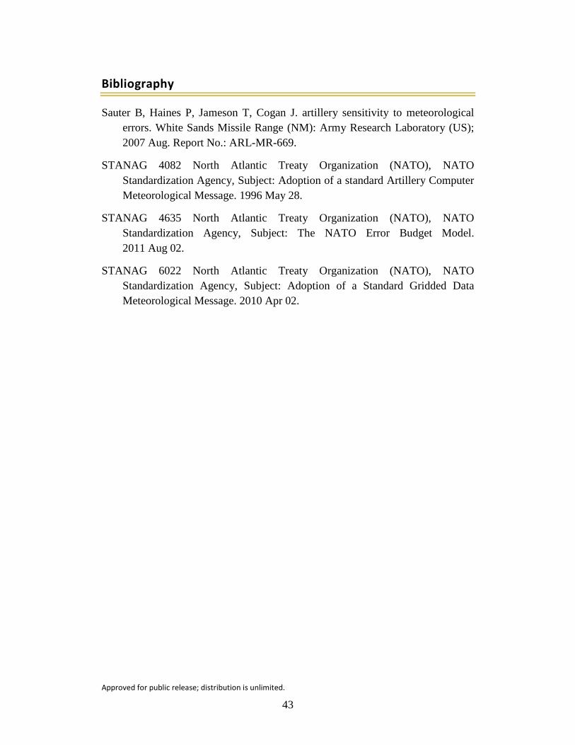
Bibliography

Sauter B, Haines P, Jameson T, Cogan J. artillery sensitivity to meteorological errors. White Sands Missile Range (NM): Army Research Laboratory (US); 2007 Aug. Report No.: ARL-MR-669.

STANAG 4082 North Atlantic Treaty Organization (NATO), NATO Standardization Agency, Subject: Adoption of a standard Artillery Computer Meteorological Message. 1996 May 28.

STANAG 4635 North Atlantic Treaty Organization (NATO), NATO Standardization Agency, Subject: The NATO Error Budget Model. 2011 Aug 02.

STANAG 6022 North Atlantic Treaty Organization (NATO), NATO Standardization Agency, Subject: Adoption of a Standard Gridded Data Meteorological Message. 2010 Apr 02.


44

List of Symbols, Abbreviations, and Acronyms

3DVAR 3-dimensional variational

4DVAR 4-dimensional variational

557th WW 557th Weather Wing

AFWA Air Force Weather Agency

AGL above ground level

ARL US Army Research Laboratory

CMD-P Computer Meteorological Data-Profiler

DA data assimilation

EnKF ensemble Kalman filter

FDDA 4-dimensional data assimilation

GBS Global Broadcast System

GFS Global Forecast System

MET meteorological

METCM meteorological computer message

NWP Numerical Weather Prediction

obs observation(s)

OI optimal interpolation

PBL planetary boundary layer

PVM Profiler Virtual Module

SQL Standard Query Language

UTC Coordinated Universal Time

VS verifying soundings

WMO World Meteorological Organization

WRF Weather Research and Forecasting


45

Z Zulu

YPG Yuma Proving Ground


46

1 DEFNS TECHL INFO CTR (PDF) DTIC OCA 2 DIRECTOR (PDF) US ARMY RSRCH LAB RDRL CIO LL IMAL HRA MAIL & RECORDS MGMT 1 GOVT PRINTG OFC (PDF) A MALHOTRA 5 US ARMY RSRCH LAB (PDF) ATTN RDRL CIE M PA HAINES JA SMITH BP REEN JL COGAN RW HORNBAKER (SSI) 1 CACI (PDF) DJ EPLER 1 PENN STATE UNIVERSITY (PDF) DEPARTMENT OF MET DR STAUFFER 2 OFFICE OF PRODUCT (PDF) DIRECTOR FSC2 SFAE CCC MCF R HUDUK K LY 1 FD PROJECT LEAD (PDF) D CAMPOS-BARAHONA 1 PROFILER ACTION OFFICIER (PDF) CDID TCM FIRES CELLS EE EDKIN 1 SENIOR PROGRAM ANALYST (PDF) KNOWLEDGE CAPITAL

ASSOC LLC S MITCHELL

Documents

Testing the Data Assimilation Capability of the Profiler