Testing the Determinants of Corruption from Multiple

Testing the Determinants of Corruptionfrom Multiple Theoretical Lenses:The Case of the U.S. States

Development Studies Series 26

Cheol Liu, Can Chen

Testing the Determinants of Corruptionfrom Multiple Theoretical Lenses:The Case of the U.S. States

Cheol Liu, Associate Professor, KDI School of Public Policy and [email protected]

Can Chen, Assistant Professor, Florida International University [email protected]

Abstract

This article compares the determinants of public corruption from multiple

theoretical lenses and then tests which ones are more effective in curbing

public corruption in the context of the U.S. states. We find that the

stringency of state tax and expenditure limits, fiscal transparency, voter

turnout rates, unified Democratic control, divided control of state governments,

political competitiveness, population with Scandinavian ancestry, and

educational attainment are all significantly and negatively associated with the

extent of public corruption. Compared with other approaches to curbing

corruption (i.e., the lawyer’s approach, the businessman’s approach, and the

economist’s approach), those that restrict public officials’ discretionary power

and encourage educated citizens’ participation appear to be more effective in

reducing corruption in the U.S. states.

Keywords

Corruption; Comparison of multiple theories; Determinants and cures for corruption

INTRODUCTION

This article compares various theoretical determinants of public corruption from the

perspective of their effectiveness in curbing corruption. For this comparison, we review the

existing literature related to the determinants and cures for corruption across countries, and

test which among those suggested by multiple theoretical approaches are the more effective

ones for reducing public corruption in the context of the U.S. states. Lopez-Iturriaga and

Sanz (2018) find that most existing corruption studies discussing the causes of corruption

tend to focus on cross-country comparisons and, therefore, call for further studies

employing within-country data and contexts.

One of the major challenges of corruption-related studies is the difficulty in defining

corruption and choosing practical measures of corruption for quantitative research with a

large N. Corruption is broadly understood as deviation from the rational-legal Max

Weberian bureaucracy. Lancaster and Montinola (1997) categorize various definitions of

corruption according to six broad meanings: 1) corruption implies public officials’

behaviors deviating from the public interest (public interest-centered definition), 2)

corruption means public officials’ behaviors that are different from legal norms (public

office-centered definition), 3) corruption involves public officials’ behaviors deviating not

only from legal norms but also from moral norms (public norm-based definition), 4)

patrimonialism implies “a form of domination with an administrative apparatus whose

members are recruited from personal dependents of the ruler”, 5) corrupt public officials

regard their public office as their private business (market-oriented definition), and 6) all

public officials’ behaviors deviating from the ideal principal-agent relationship are defined

as corruption. A long debate on the definition of corruption has led to a consensus that

corruption refers to public officials who engage in behaviors that use their public office,

authority, and power for their personal gain. Corruption also involves various elements of

nepotism, clientelism, favoritism, misuse of public power, patronage appointment, and moral

decay. Among the various definitions, the strictest one defines corruption as deviation from

formal rules regulating public workers’ behaviors. Because corruption occurs clandestinely,

it cannot be openly measured. Thus, most empirical studies capture the extent of corruption

by measuring the perceived degree of corruption instead of the actual level of corruption

(Lancaster and Montinola, 1997, 188-191).

The existing literature on corruption generally concurs that it is not possible to specify

a complete and comprehensive definition of corruption. It is also impossible to develop a

Testing the Determinants of Corruption from Multiple Theoretical Lenses: The Case of the U.S. States 5

comprehensive list of corruption practices that is universally applicable to all societies over

a long period of time. Different societies have different perceptions, cultures, and rules in

relation to corruption, which also change over time even within a society. The term

definitional quagmire expresses the difficulty in seeking a complete and universal definition

of corruption and constructing a comprehensive measure of the actual level of corruption

(Johnston, 1994). Thus, it is suggested that researchers might apply a useful definition and

a practically available measurement of corruption that are appropriate for their specific

research concerns and contexts, rather than becoming stalled in a quagmire of seeking

perfect definitions and measurements of corruption (Collier, 1999; Kaufmann, 1998).

Following in the tradition of corruption studies, this article limits the category of

corruption to its strictest definitional sense, namely, deviation from formal rules regulating

public officials’ behaviors. We capture the extent of corruption through the number of

public officials who are convicted of the violations of the corruption-related laws within a

country. Additionally, we argue that the number of convictions should be a better indicator

of corruption than the number of indictments and caseloads. This is because it is possible

that a number of indictments and accusations will eventually be dismissed by the courts

and not convicted as corruption. We thus assume that convicted cases correspond to

corruption cases.

This article proceeds as follows. The next section reviews relevant literature on

corruption and establishes the theoretical framework of the study. We then present the data

and develop empirical models to test the explanatory power of multiple theoretical lens

related to corruption. Next, we report the empirical results of the models and conclude by

discussing the implications of our research findings.

MULTIPLE THEORETICAL LENSES FOR EXPLAINING

CORRUPTION

This study makes use of a comprehensive review of the literature on corruption1).

Most of the research reviewed involved cross-country studies. Amongst them, this article

focuses on the theories that are applicable to a within-country study, particularly in the

context of the U.S. states.

Public choice theorists argue that public officials, like private individuals, make choices

1) We tabulate the comprehensive list of the existing literature in the Appendix (Tables A1~A4) for brevity.

to maximize their private self-interest (Buchanan and Tullock 1962; Niskanen 1971). A

public official is portrayed as a rational utility maximizer who could engage in corruption

when the potential benefit from corruption exceeds its potential cost (Rose-Ackerman and

Palifka 2016; De Graaf 2007). The theorists presume that maximizing the cost of

corruption and minimizing its potential benefit should deter or at least reduce unethical

behavior. We summarize discussions of the determinants of corruption from multiple

theoretical lenses and from the perspective of this benefit/cost comparison approach.

Bureaucratic Determinants of Corruption

Public bureaucrats are susceptible to corruption when “there is a lot of money lying

around loose and no one is watching” (Wilson 1966, 31). Bureaucratic explanations of

corruption are related to opportunities for corruption, including the following five key

factors: bureaucratic regulation, size of bureaucracy, bureaucratic structure (fragmentation

and decentralization), wages, and fiscal institutions to constrain the power of public

officials.

With reference to the first factor, the public interest model of bureaucratic regulation

assumes that regulation counteracts market failures and is instituted by government officials

to maximize the general welfare (Pigou 1938). However, the public choice literature on

bureaucratic regulation suggests that regulations are captured by the regulated industries and

usually benefit existing larger firms (Stigler 1971; Tullock 1967). Similarly, politicians and

bureaucrats cater to business interest in order to maximize their private self-interests and

use excessive bureaucratic regulations as a tool to extract larger bribes. Shleifer and

Vishny (1993) argue that many regulations exist to give public officials “the power to

deny them and to collect bribes in return for providing the permits” (601). When

regulation is stricter and license approval processes are slower, private businesses are more

likely to bribe government officials to avoid regulatory cost. Djankov et al. (2002) find

that various measures of firm entry regulation are positively associated with the level of

corruption in a cross-country sample.

For the second factor, as the size of government (bureaucracy) increases, opportunity

for corruption also increases. In addition, the size of government associates positively with

the size of rent from corruption. A larger size of government means a greater amount of

bureaucratic delay and induces rent-seekers to offer larger bribes (Goel and Nelson 1998).

As Scully (1991) asserts, “The increase in the size and scope of government expenditure

represents an enormous rise in the opportunities for rent-seeking through budgetary


reallocations” (91). Goel and Nelson (1998) also find that government size, in particular,

spending by the U.S. state governments, does indeed have a strong positive association

with corruption.

The third factor, namely, the structure of bureaucracy, is also perceived to affect

corruption. A more fragmented structure of government makes corruption less visible,

which reduces the chance of corrupt officials being detected. Fragmentation also impedes

coordination among public officials and incentivizes them to overgraze the common bribe

base (Goel and Nelson 2011). Henriques (1986) argues that the fragmentation of

government resulting from the proliferation of single purpose special districts stimulates

corruption. On the contrary, the decentralization of government brings public officials closer

to the people and stimulates inter-jurisdictional competition among governments for mobile

resources, which enhances government accountability and discipline and, as a consequence,

reduces corruption (Klitgaard 1988).

Concerning the fourth factor, Becker and Stigler (1974) maintain that bureaucratic

wages should be related to corruption. If public employees earn less than they could earn

in the private sector, the probability of their committing corruption increases. However, a

wage increase in the public sector reduces the need for corruption and makes bribe taking

less attractive. Moreover, higher pay in the public sector makes it possible to attract and

retain better qualified, more professional, and less corrupt public employees (Cornell and

Sundell 2019).

For the fifth factor, most fiscal institutions intend to constrain public officials’ fiscal

discretion and reduce corruption. The Leviathan model argues that government officials are

self-interested and maximize discretionary budget slack for private gains (Niskanen 1971,

1975). Fiscal institutions serve as ex-ante rules that limit the policy choices of government

officials and bind Leviathan because they prescribe what politicians can and cannot do

(e.g., Chan and Mestelman 1988; Moene 1986). A harder budget constraint will lower

budgetary slack (Borge et al. 2008). Tax and expenditure limitations (TELs) and balanced

budget requirements of the state and local governments in the U.S. aim to limit the

growth of government and impose fiscal discipline on public officials. TELs are expected

to reduce opportunities for corruption by constraining government expenditure and revenue.

Budgetary institutions aiming for transparency are also likely to reduce corruption.

Transparency increases the chance that corruption will be detected. If budgets and other

financial documents are transparent and available for all to see, it is more difficult for

public officials to distort information and conceal their corruption (Anechiarico and Jacobs

1996; De Graaf 2007). From the perspective of the principal-agent theory, transparent

environments reduce information asymmetries between public officials and voters, and help

align the interests of agents with those of principals. Transparency induces governments to

report both their planned budgets and their actual execution to citizens so that the public

(and its watchdogs) can monitor the budget process more effectively. This enhances public

oversight on the allocation and spending of public resources, and leaves less room for

agents to abuse public resources for their private gain (Blinded 2019).

Political Determinants of Corruption

Political explanations of corruption contend that politics can curb corruption if political

actions raise the cost of corruption by increasing the probability that corruption will be

detected and penalized. In this regard, the key factors discussed in the existing literature

are political competition, citizen voting, gubernatorial term limit, and political ideology.

Rose-Ackerman (1978) presents one of the most influential theories about the effect of

political competition on corruption. When the level of political competition is low, political

incumbents are more confident of their re-election and less motivated to hold accountability

for their behaviors. It is possible for them to seek rent without being voted out of their

office. However, a higher level of political competition (e.g., closely contested political

elections) mobilizes critical voters and intensifies the need to scrutinize current government

by opposing parties. This restricts elected officials’ incentives to use their office for private

gain. Likewise, divided government is associated with a lower level of corruption because

power sharing among political incumbents represents a variation of political competition.

The political agency model posits that citizens (the principals) delegate authority to

elected officials (the agents) to act on their behalf and in their interest (Barro 1973;

Ferejohn 1986; Persson et al. 1997). Yet voters and politicians face conflicting motivations

and incentives. Voters pay taxes to finance the provision of public goods and services.

Politicians can extract rent from tax revenue collected, thus leaving fewer funds for public

good provision. If voters perceive the current level of rent as too high, they vote the

incumbent out of office (retrospective voting). However, this kind of vertical accountability

works only if voters are actively involved in elections. An informed and active electorate

enhances the probability that corrupt politicians will be punished for their corruption.

Ferejohn (1986) states that achieving vertical accountability becomes harder in a

multidimensional policy space because various voters would use their one vote to decide

issues in different policy dimensions. Institutions such as citizen initiatives that reduce the


dimensionality of policy space help voters hold politicians more accountable, which results

in a lower level of rent and corruption (Alt and Lassen 2003).

Gubernatorial term limits are expected to associate negatively with corruption. Given

that governors in office are banned from holding their office again due to term limits, they

are more likely to fight corruption to preserve not only their parties’ reputation but also

their individual reputation (Escaleras and Calcagno 2009).

Finally, Meier and Holbrook (1992) underline the effect of political ideology on

corruption, although conflicting arguments for the association are possible. Conservative

citizens often perceive politics as means of seeking self-interest of public officials, so they

tend to be more tolerant of officials’ unethical behaviors. This encourages public officials

to believe that the probability of being penalized for their corruption might be low. In

contrast, conservatives who are strongly against larger governments tend to favor policies

and laws to fight against waste, inefficiency, and corruption in public programs.

Economic and Demographic Determinants of Corruption

Economic and demographic determinants of corruption are dominant factors according

to the existing literature on corruption. These include level of income, income inequality,

ethnic diversity, and female population. As the level of income increases in a society, the

demand for corruption falls. In addition, a rise in income will make more resources

available to curb corruption. It has been found that a high level of income has a

significantly negative effect on corruption (e.g., Damania et al. 2004; Persson et al. 2003).

On the contrary, a higher extent of income inequality is positively associated

corruption for two reasons. First, the chance of being caught for a corrupt behavior is

lower with a higher extent of income inequality because people who are at the lower end

of the income spectrum are largely unaware and incapable of monitoring public officials.

Second, when income inequality is higher, the benefit of corruption becomes greater for

wealthy persons. However, the cost of corruption becomes lower because resources

available for the masses of poor people to hold public officials accountable are constrained

(Jong-Sung and Khagram 2005). Paldam (2002) argues that “a skewed income distribution

may increase the temptation to make illicit gains” (224).

Ethnic diversity is associated with a higher level of corruption. Members of a certain

ethnic group often favor their group members over non-members (Vanhanen 1999). When

there are multiple ethnic groups in a society, public officials tend to allocate resources

towards supporters of their own ethnicity. Ethnic groups are more likely to support public

officials of their own ethnicity even if they are known to be corrupt (Glaeser and Saks

2006, 8). Ethnic diversity “rationalizes corruption extraction from others unlike self”

(Maxwell and Winter 2004, 18).

Finally, it is argued that the share of women in total population correlates with a

lower level of corruption. Women are more trustworthy and more risk averse than men.

Thus, they are willing to follow rules and feel there is a greater probability of being

caught for corruption, which results in a lower level of corruption (Swamy et al. 2001).

Historical and Cultural Determinants of Corruption

Historical and cultural explanations of corruption point out that historical and cultural

traditions might affect the perceived cost of corruption. The key determinants of corruption

from this perspective include urbanization, education, social capital, and immigration.

Historically, urban environments foster conditions that are conducive to corruption. The

social control of family and religion becomes weaker in urbanized areas, and government

programs and resources are concentrated more in urbanized areas. In an urbanized

environment, moreover, political machines tend to be established to “benefit individuals

who supported the urban political machine, and corruption was used to compensate

machine operators for their efforts” (Meier and Holbrook 1992, 138). Cities provide more

opportunities for corruption than rural areas.

The cultural explanations of corruption center on popular psychology. As Wilson

(1966) asserts, “There is a particular political ethos or style which attaches a relatively low

value to probity and impersonal efficiency and relatively high value to favors, personal

loyalty, and private gain” (30). The middle-class reformers seek to eliminate the traditional

political ethos and fight for a clean government. Meier and Holbrook (1992) argue that the

middle-class preference opposing corruption can be captured by the education levels of the

population. Well-educated citizens are less tolerant of corruption and more likely to push

public officials to be more accountable.

Corruption thrives in an environment where pro-social norms such as trust and altruism

are absent (Banerjee 2016). The lack of social trust may diminish the sense of wrongdoing

and neglect corruption in the society (Rotondi and Stanca 2015), which in turn breeds

even more corruption (Banerjee 2016). According to Persson et al. (2013), citizens’

willingness to control corruption depends largely on their expectation of how many people

in their society are engaged in corruption. If the majority perceives corruption as a

widespread social norm, citizens are less likely to monitor and sanction corruption. Thus, a


higher level of social capital can increase citizens’ willingness and cooperation to control

corruption.

Lastly, immigration is often associated with a higher level of corruption. Immigrants

from a society with a higher level of corruption may import their culturally corrupt

baggage and provide more opportunities for corruption in the destination society. They also

have fewer economic resources to lose and might perceive the cost of corruption as lower

(Meier and Holbrook 1992).

DATA, MODEL, & METHODOLOGY

Model Specification

Based on the multiple theories of corruption discussed in the previous section, we

construct a regression model of the determinants of corruption in the context of the U.S.

states as follows:

= 0 + 1 ( _ ) + 2 ( ) + 3 ( _ ℎ ) + 4 ( _ ) + + + In our model, is the observed level of corruption at state i in year t. The extent of

corruption across the 50 states is captured both by the number of convictions per 10,000

public employees and the number of convictions per 100,000 people of state population.

The U.S. Department of Justice annually publishes the number of federal, state, and local

employees who are convicted of federal corruption-related laws in a document entitled

Report to the Congress on the Activities and Operations of the Public Integrity Section.

The reliability, relevance, and validity of the conviction measures have been discussed by

many scholars and studies (e.g., Butler, Fauver, and Mortal 2009; Cordis and Milyo 2016;

Glaeser and Saks 2006; Meier and Holbrook 1992; Zhang and Kim 2017). We estimate

the extent of corruption in year t in three ways: the number of convictions in year t, the

number of convictions in year (t+1), and the average number of convictions in years (t+1),

(t+2), and (t+3). We use the lead values of the numbers of convictions, or those in years

(t+1),(t+2), and (t+3) to capture the extent of corruption in year t, as it is possible that

corruption cases convicted in year t actually took place in the previous years, not in year t.

Bureaucratic_Regulatory it is a vector of variables capturing state bureaucratic and

regulatory determinants of corruption. They include the degree of bureaucratic regulation,

the number of state public employees, the average level of state public employees’ wages,

the extent of fiscal decentralization, the degree of state government fragmentation, the

stringency of TELs, the stringency of state balanced budget rules, and the degree of state

budget transparency.

Political it represents a set of political factors assumed to affect state corruption. These

include voter turnout rates, the extent of state political competition, political ideology of

citizens, political ideology of state governments, a dummy of term limit for governors, a

dummy of citizen initiatives, a dummy of unified Democratic control of state governments,

a dummy of unified Republican control of state governments, and a dummy of politically

divided control of state governments.

𝐸𝑐𝑜𝑛𝑜𝑚𝑖𝑐_ 𝐷𝑒𝑚𝑜𝑔𝑟𝑎𝑝ℎ𝑖𝑐𝑖𝑡 is a vector of economic and socio-demographic drivers of

state corruption. This determinant captures the level of personal income per capita, the

extent of income inequality, the degree of ethnic diversity, and the percentage of female

citizens in state population.

𝐻𝑖𝑠𝑡𝑜𝑟𝑖𝑐𝑎𝑙 _ 𝐶𝑢𝑙𝑡𝑢𝑟𝑎𝑙 𝑖𝑡 denotes the factors related to historical, cultural, and religious

explanations of state corruption. These include the extent of educational attainment, social

capital index, Scandinavian ancestry (%), and the percentage of urban population.

𝜃𝑖 implies state fixed effect to control for unobservable state attributes, is the

time-specific effect to control for yearly changes in state external environment over 23

years in the period 1986-2008, and is the random error term. Table I displays the detailed

descriptive statistics of all variables, shows how to capture them, and where we collected

the data.


Table I. Descriptive Statistics: Variable Definition, Summary Statistics, and Data Sources

Variable Definition Mean SD Min Max Data Source

CorruptempNumber of state corruption-related convictions per 10,000 public employees

0.51 0.42 0 2.7U.S. Department of Justice

CorruptpopNumber of state corruption-related convictions per 1,000,000 residents

0.33 0.30 0 2.5U.S. Department of Justice

Bureaucratic Regulation

The regulation sub-index of state economic freedom index

4.81 1.33 0.7 8.7 The Fraser Institutions

Number Gov’t Employees

Number of state government full-time employees

11.51 1.63 8.1 16.9U.S. Bureau of Economic Analysis

Gov’t Employee Wages

Average payroll for state full-time employees


Fiscal Decentralization

The ratio of state expenditures to the sum of state and local government expenditures.

0.32 0.07 0.1 0.7U.S. Census Bureau State and Local Government Finance

Gov’t Fragmentation

The number of general-purpose local governments (counties, cities, township) per 1,000,000 residents

271.66 457.28 3.0 2797.2U.S. Census Bureau State and Local Government Finance

TELs StringencyAn index that measures the restrictiveness of state tax and expenditure limits (TEL)

24.13 8.08 0 32 Amiel et al. (2009)

Balance Budgets Stringency

A variable that measures the stringency of state balanced budget rules (BBR). It ranges from 0 to 10, with higher values indicating stricter rules.

7.35 2.97 0 10Krause and Melusky (2012)

Fiscal Transparency An index that measures the degree of fiscal transparency of state budgeting processes

0.51 0.19 0.1 1Alt, Lassen, and Rose (2006)

Voter Turnout Rates

Percentage of the voting-eligible population turnout rate for the highest office election

12.42 12.57 1.0 74 U.S. Election Project

Political Competition

The folded Ranney index measures interparty competition of governmental partisan control, ranging from 0.5 to 1. The larger the value is, the greater the interparty competition.

0.88 0.10 0.6 1 Klarner (2012)

Citizen Liberal Ideology

Berry et al. (1998) measure U.S. states’ political ideology.

50.53 15.11 8.4 96 Berry et al. (1998)

Gov’t Liberal Ideology

Berry et al. (1998) compute a weighted average of the ideology scores to measure state government’s political ideology.

50.74 25.58 0 98 Berry et al. (1998)

Governor’s Term Limits

A dummy variable that indicates whether a governor is subject to term limits

0.72 0.45 0 1 The Book of States

Citizen Initiative Dummy

A dummy variable that indicates whether a state allows for citizen initiative

0.53 0.50 0 1The Correlates of State Policy Projects

Unified Demo Control

A dummy variable that indicates unified Democratic control of state governments

0.23 0.42 0 1 Klarner (2012)

Unified Republican Control

A dummy variable that indicates unified Republican control of state governments

0.18 0.39 0 1 Klarner (2012)

Estimation Method

Due to the panel data structure, we employ a two-way panel estimator with state and

year dummies to control both state and year-invariant unobserved heterogeneity. The

variance inflation factor (VIF) test finds that the mean value of the VIF test is 3.63. VIFs

for all variables are less than 10, which implies that multicollinearity is not a serious

problem for this study. A series of panel unit root tests show that the dependent variables

are panel stationary, and thus fixed effect or random effect models are applicable to our

analysis and their results are not spurious. It is known that if a panel is stationary, then a

static panel data method should be applied; otherwise, a dynamic specification should be

used. We use two kinds of tests, namely, the Augmented Dickey-Fuller test and the

Phillips-Perron test, with different specifications on lags, a linear trend, or a drift for all

three dependent variables. All specifications reject the null hypothesis of unit root.

Hausman tests are performed to test the specification of fixed-effect versus random-effect

model. The null hypothesis, which states that the difference of the coefficients estimated

by the two specifications is not systematic, is rejected, thus indicating the choice of a

fixed-effect model is suitable.

We also conduct some conventional initial diagnostic tests before running the

regressions. First, the Breusch-Pagan/Cook-Weisberg test confirms that the estimated

Variable Definition Mean SD Min Max Data Source

Divided Gov’t

A dummy variable indicating that the control of the executive branch and the legislative branch is split between two parties

0.58 0.49 0 1 The Book of States

Real Personal Income

Natural log of real per capita personal income


Income Inequality (Gini)

Measure of income inequality ranging from 0 (perfect equality) to 1 (perfect inequality)

0.43 0.04 0.3 0.5The Correlates of State Policy Projects

Ethnic DiversityAn index measure of racial diversity that varies over time and across states

0.23 0.13 0.0 0.7Hawes, Rocha, and Meier (2013)

Female Pop (%)Percentage of females in state population

0.51 0.02 0.5 0.7 U.S. Census Bureau

Educational Attainment

Percentage of bachelor's degrees or higher for persons 25 years or over


Social CapitalAn index measure of social capital that varies over time and across states

0.14 0.98 -2.9 2.7Hawes, Rocha, and Meier (2013)

Scandinavian Ancestry (%)

Percentage of population with Scandinavian ancestry

9 3.39 2.9 19.7 U.S. Census Bureau

Urban Population (%)

Percentage of population residing in urban areas

70.49 14.68 32.2 94.9 U.S. Census Bureau


residuals are heteroskedastic. Second, the Wooldridge test confirms the existence of serial

correlation in error terms. Third, the Pesaran’s cross-sectional dependence (CD) test

confirms the existence of cross-sectional dependence. Heteoskedasticity, serial correlation,

and cross-sectional dependence will yield biased standard errors of estimated coefficients.

To correct the above issues, we use the Driscoll and Kraay standard errors as Driscoll and

Kraay (1998) suggest.

EMPIRICAL FINDINGS

We run two rounds of regressions of the determinants of public corruption in the U.S.

states. In the first round, our regression models separately include each set of the

determinants of corruption one by one. We have four sets of the public corruption

determinants: bureaucratic and regulatory determinants, political determinants, economic and

demographic determinants, and geographical, cultural, and religious determinants. The

second round of regressions includes all four sets of the determinants together. For brevity,

we do not report the regression results of the first round in detail,2) but summarize which

determinants are statistically significant in what follows. We only report the regression

results of the second round in the body of this article and discuss the main findings.

The results of the first round of regressions are summarized as follows. The positive

(+) and negative (-) signs in parentheses imply the directions of the association between

each determinant and the dependent variable (i.e., public corruption). Among the

bureaucratic and regulatory determinants of corruption, the number of state public

employees (+), the stringency of TELs (-), and the stringency of BBRs (-) are statistically

significantly associated with corruption in the context of the U.S. states. Among the

political determinants of corruption, voter turnout rates (-), political competition (-), the

liberal ideology of state governments (+), the existence of a term limit for governors (-),

unified control of state governments by Democrats (-), and divided controls of state

governments (-) are significant factors of corruption. Among the economic and demographic

determinants of public corruption, only income inequality (+) is significantly associated

with corruption. Finally, educational attainment (-) and Scandinavian ancestry (-) are

statistically significant and negatively associated with the extent of corruption.

At the second round of regressions, we combine all four sets of the determinants of

2) Tables A.5~A.0 in the Appendix display the regression results in greater detail.

public corruption, not separating them. Table II summarizes the regression result of our

benchmark models, which show that the regression results are consistent with those of the

first round of regressions. We have six different models (Models I~XI) in Table II with

different dependent variables (i.e., the measurements of the extent of corruption across the

states). The first three models capture the extent of public corruption by the number of

convictions per 10,000 state public employees (Corruptemp) at year t (Model I), at year

t+1 (Model II), and average numbers over future three years (Model III). The last three

models capture the level of public corruption by the number of convictions per 100,000

state population (Corruptpop) at year t (Model IV), at year t+1 (Model V), and average

numbers over the future three years (Model VI). We use shading to emphasize

determinants that show statistically significant associations with corruption. The result of

estimation looks consistent over all six models, as we summarize below.

There is a positive association between the number of public employees and the extent

of public corruption in the context of the U.S. states, which is statistically significant at

the 0.1% significance level. Public corruption is likely to be higher in a state with a larger

number of public employees. We may also interpret this result as providing evidence

supporting a theoretical argument that corruption should tend to increase as the size of the

public sector increases, as we use the number of public employees as a proxy for the size

of the public sector, following Dimant and Tosato (2018) and Kotera et al. (2012).

A U.S. state with a tighter stringency of state TELs is likely to have a lower degree

of corruption, which is statistically significant at the 1% and/or 0.1% significance levels. A

negative association between BBRs and corruption does not seem significant. Although the

impacts of regulation on corruption are controversial across the existing studies, we find

that state TELs reduce the extent of corruption by constraining public employees’

discretion on resource allocation in the context of the U.S. states. Likewise, it seems that

a U.S. state government with a higher level of fiscal transparency is likely to have a

lower level of corruption.

There is a negative association between voter turnout rates and corruption in the

context of the U.S. states, which is statistically significant at the 0.1% significance level.

We use voter turnout rates as proxies for the development of democracy or/and degree of

citizens’ participation in politics. Public corruption tends to become lower in a state with a

higher level of democracy and/or a higher degree of citizens’ participation because corrupt

politicians are removed by elections (e.g., Bhattacharyya and Hodler 2015).

Citizens’ liberal political ideology and unified Democratic controls tend to have a


negative association with the extent of corruption. Moreover, a U.S. state with a stronger

degree of political competition is likely to have a lower level of corruption, which is

statistically significant at the 0.1% significance level. This finding is consistent with the

result from the variable of divided control of state governments. Competition for political

positions helps politicians to avoid self-seeking behavior and, as a consequence, reduce

corruption (Brown et al. 2005; Sharafutdinova 2010).

A state with a higher level of income inequality tends to have a higher level of

corruption. In contrast, a state with a higher extent of educational attainment and a higher

percentage of population with Scandinavian ancestry is likely to have a lower extent of

corruption. We capture the level of educational attainment across the states by calculating

the percentages of state population acquiring a bachelor’s degree or higher for people who

are 25 years of age or older. The role of education matters in reducing public corruption

in the context of the U.S. states (Brunetti and Weder 2003; Truex 2011).

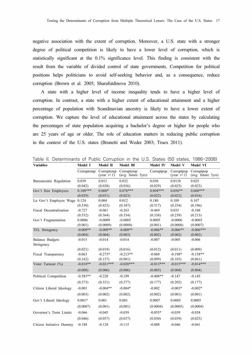
Table II. Determinants of Public Corruption in the U.S. States (50 states, 1986-2008)Variables Model I Model II Model III Model IV Model V Model VI

Corruptemp Corruptemp(year t+1)

Corruptemp(avg. future 3yrs)

Corruptpop Corruptpop(year t+1)

Corruptpop(avg. future 3yrs)

Bureaucratic Regulation 0.039 0.013 0.032 0.030 0.0138 0.025(0.042) (0.038) (0.036) (0.029) (0.025) (0.023)

Gov’t Size Employees 0.108*** 0.060* 0.078*** 0.094*** 0.056** 0.068***(0.029) (0.031) (0.023) (0.022) (0.022) (0.016)

Ln Gov’t Employee Wage 0.124 0.004 0.012 0.180 0.109 0.107(0.530) (0.423) (0.347) (0.317) (0.254) (0.196)

Fiscal Decentralization -0.727 -0.061 -0.263 -0.469 0.035 -0.108(0.532) (0.364) (0.334) (0.338) (0.239) (0.213)

Gov’t Fragmentation 0.0006 -0.0009 -0.0005 0.0005 -0.0006 -0.0003(0.001) (0.0009) (0.0009) (0.001) (0.0008) (0.0007)

TEL Stringency -0.009** -0.009** -0.009** -0.006** -0.006** -0.006***(0.004) (0.004) (0.003) (0.002) (0.002) (0.002)

Balance Budgets Stringency

-0.015 -0.014 -0.014 -0.007 -0.005 -0.006

(0.021) (0.019) (0.016) (0.012) (0.011) (0.009)Fiscal Transparency -0.063 -0.273* -0.213** -0.060 -0.198* -0.158**

(0.162) (0.157) (0.081) (0.099) (0.103) (0.061)Voter Turnout (%) -0.018** -0.021*** -0.020*** -0.013*** -0.015*** -0.014***

(0.008) (0.006) (0.006) (0.005) (0.004) (0.004)

Political Competition -0.583** -0.228 -0.199 -0.408** -0.147 -0.145

(0.273) (0.321) (0.277) (0.177) (0.202) (0.177)

Citizen Liberal Ideology -0.003 -0.004** -0.004* -0.002 -0.003* -0.002*

(0.003) (0.002) (0.002) (0.002) (0.001) (0.001)

Gov’t Liberal Ideology 0.001* 0.001 0.001 0.0007 0.0005 0.0005

(0.0007) (0.001) (0.001) (0.0004) (0.0005) (0.0004)

Governor’s Term Limits -0.066 -0.045 -0.039 -0.055* -0.039 -0.038

(0.046) (0.057) (0.037) (0.030) (0.039) (0.025)

Citizen Initiative Dummy -0.188 -0.128 -0.115 -0.088 -0.046 -0.041

DISCUSSION AND CONCLUSION

Table III summarizes the regression results of our benchmark models (Models I~VI in

Table II) and compares the determinants of public corruption suggested from multiple

theoretical lenses. In the context of the U.S. states, the number of public employees and

the degree of income inequality are positively associated with the level of state corruption.

On the contrary, the stringency of state TELs, the degree of fiscal transparency, voter

turnout rates, unified Democratic control, politically-divided control of state governments,

the extent of political competitiveness, the percentage of population with Scandinavian

ancestry, and the level of educational attainment are negatively associated with the extent

of state corruption. We do not find statistically significant associations between the level of

state public corruption and multiple variables suggested as significant determinants of

public corruption from multiple theoretical lenses. These include the level of public

employees’ wages, fiscal decentralization, the degree of government fragmentation, index of

Variables Model I Model II Model III Model IV Model V Model VI

Corruptemp Corruptemp(year t+1)

Corruptemp(avg. future 3yrs)

Corruptpop Corruptpop(year t+1)

Corruptpop(avg. future 3yrs)

(0.193) (0.166) (0.104) (0.132) (0.118) (0.077)

Unified Demo Control -0.143*** -0.149** -0.111*** -0.095*** -0.089** -0.068***(0.037) (0.056) (0.036) (0.025) (0.038) (0.024)

Unified Republican Control

-0.026 -0.091 -0.053 -0.025 -0.071 -0.044*

(0.036) (0.068) (0.039) (0.026) (0.046) (0.024)Divided Gov’t -0.078** -0.141** -0.104*** -0.054** -0.093** -0.068**

(0.035) (0.066) (0.037) (0.021) (0.045) (0.025)Ln Real Personal Income -0.055 -0.329 -0.067 0.088 -0.206 0.014

(0.409) (0.342) (0.320) (0.289) (0.223) (0.218)Income Inequality (Gini) 1.388* 1.526** 1.551*** 1.049** 1.026** 1.070***

(0.704) (0.631) (0.347) (0.445) (0.390) (0.193)Ethnic Diversity 0.087 0.051 0.027 0.074 0.038 0.022

(0.069) (0.066) (0.034) (0.045) (0.049) (0.024)Female Pop (%) 0.121 -0.314 -0.610 0.358 0.037 -0.171

(0.547) (0.782) (0.510) (0.394) (0.551) (0.365)Educational Attainment -0.038*** -0.048*** -0.040*** -0.027** -0.032*** -0.027***

(0.014) (0.013) (0.008) (0.010) (0.010) (0.006)Social Capital Index -0.004 0.019 0.0155 2.39e-05 0.013 0.011

(0.034) (0.034) (0.022) (0.022) (0.024) (0.015)Scandinavian Ancestry (%) -0.040** -0.025 -0.030*** -0.025** -0.016 -0.020***

(0.019) (0.019) (0.009) (0.012) (0.013) (0.006)Urban Population (%) -0.003 -0.001 -0.0003 -0.001 -0.0003 7.48e-05 (0.006) (0.005) (0.004) (0.004) (0.003) (0.00276)State Fixed Effects Yes Yes Yes Yes Yes YesTime Fixed Effect Yes Yes Yes Yes Yes YesN 1,150 1,150 1,150 1,150 1,150 1,150R-squares 0.1035 0.1046 0.1584 0.0982 0.0956 0.146


BBRs, citizens’ liberal ideology, government’s liberal ideology, existence of term limits for

governors, citizen initiatives, unified Republican control of state government, per capita

personal income, ethnic diversity, percentage of female population, social capital index, and

the percentage of population residing in urban areas.

Table III. Comparison of the Determinants of Corruption in the Context of the U.S. States

Theoretical Approach Positive (+) Negative (-) Insignificant

Bureaucratic andregulatory determinants

Size of publicemployees*(government size)

Stringency index of state TELs*Fiscal transparency

Gov’t employee wageFiscal decentralizationGov’t fragmentationBBR index

Political determinants N.A.

Voter’s turnout rates*Unified democratic control*Divided government*Political competition

Citizen liberal ideology Gov’t liberal Ideology Governor’s term limits Citizen initiatives Unified Republic control

Economic anddemographicdeterminants

Income Inequality* N.A.Real personal incomeEthnic diversityFemale population (%)

Historical, cultural, andreligious determinants N.A.

Educational attainment*Scandinavian ancestry (%)

Social capital indexUrban population (%)

* Significant across all the six benchmark models displayed in Table II.

A discussion of the cures for corruption (i.e., how to reduce corruption) should start

from understanding the determinants of corruption because controlling the causes of

corruption eventually leads its prevention (Jain 2001). In this regard, multiple approaches to

reduce public corruption can be divided into three categories: the lawyer’s approach, the

businessman’s approach, and the economist’s approach. The lawyer’s approach stems from

the work of Becker (1968) and emphasizes the role of law enforcement to increase the

cost of corruption, while reducing its benefit. This approach emphasizes efforts to increase

the extent of penalties and monitoring to reduce corruption. The businessman’s approach

provides public employees with sufficient wages, incentives, and compensations so that they

might not engage in corruption. It also includes a provision of non-monetary and informal

incentives, such as career development opportunities and reputation building. Finally, the

economist’s approach focuses on reducing the discretionary power of public officials, which

can be abused for their personal gain and corruption (Ades and Di Tella 1997; Andvig

and Fjeldstad 2001).

Most existing studies fail to find a statistically significant effect of the lawyer’s

approach to reducing public corruption in the context of the U.S. states. For example, a

higher extent of law enforcement, captured by the number of state judges, the amount of

caseloads and the pending rates of state courts, working hours of the U.S. attorneys, and

the amount of state judiciary expenditures is not significantly associated with a lower level

of public corruption in the U.S. states (BLINDED, 2014). It would be worthwhile to

perform an in-depth analysis of the ineffectiveness of the lawyer’s approach to reducing

corruption in the context of the U.S.

We fail to find a statistically significant effect of the businessman’s approach in

decreasing corruption in the context of the U.S. states. As seen in Table III, the

association between the level of public employees’ wages and the extent of corruption is

insignificant. However, we should not come to the hasty conclusion that the businessman’s

approach is never effective in reducing public corruption before we make further endeavors

to investigate other possible policy instruments in line with this approach.

Compared to the former two approaches, the economist’s approach works better in

reducing corruption in the context of the U.S. states. A higher stringency of state TELs, a

higher extent of fiscal transparency, a higher degree of political competition, and politically

divided control of state governments can contribute to restricting the discretionary power of

public officials and politicians. We find that all of them are statistically significantly

associated with a lower level of public corruption in the U.S. states.

Additionally, it is noteworthy that the roles of citizens are very important in reducing

public corruption in the context of the U.S. states. We find that a U.S. state with a higher

rate of voter turnout and a higher level of educational attainment is likely to have a lower

level of corruption. Citizens’ participation in elections and their role in watching over

public officials and politicians should not be overlooked, but rather highly promoted to

reduce public corruption. Likewise, education matters in preparing citizens as active

participants of democracy.


References

Ades, A. & Di Tella, R. (1997), National champions and corruption: some unpleasant interventionist arithmetic. Economic Journal 107, 1023–42.

Anechiarico, F., & Jacobs, J. B. (1996). The Pursuit of Absolute Integrity: How Corruption Control Makes Government Ineffective. Chicago, IL: University of Chicago Press.

Andvig, Jens C., & Fjeldstad, O.H. (2001). Corruption: A review of contemporary research. Technical Report R 2001: 7. Bergen: Chr. Michelsen Institute.

Banerjee, R. (2016). Corruption, norm violation and decay in social capital. Journal of Public Economics 137, 14–27.

Barro, R. J. (1973). The control of politicians: An economic model. Public Choice 14(1), 19–42.Becker, G. (1968). Crime and punishment: An economic approaches. Journal of Political Economy

76 (2), 169–217.Becker, G. S., & Stigler, G. J. (1974). Law enforcement, malfeasance, and compensation of

enforcers. The Journal of Legal Studies 3(1), 1-18.Bhattacharyya, S., & Hodler, R. (2015). Media freedom and democracy in the fight against

corruption. European Journal of Political Economy 39, 13–24.Borge, L., Falch, T., & Tovmo, P. (2008). Public sector efficiency: The roles of political and

budgetary institutions, fiscal capacity, and democratic participation. Public Choice 136, 475-495.

Brown, D. S., Touchton, M. & Whitford, A. B. (2005). Political polarization as a constraint on government: Evidence from corruption. on SSRN http://ssrn.com/abstract=782845.

Brunetti, A. & Weder, B. (2003). A free press is bad news for corruption.” Journal of Public Economics 87(7): 1801–1824.

Buchanan, J. M., and G. Tullock. (1962). The Calculus of Consent. Ann Arbor, MI: University of Michigan Press.

Butler, A. W., Fauver, L., & Mortal, S. (2009). Corruption, political connections, and municipal finance. The Review of Financial Studies 22(7), 2873-2905.

Chan, K. S., and Mestelman, S. (1988). “Institutions, efficiency and the strategic behavior of sponsors and bureaus.” Journal of Public Economics, 37, 91-102.

Blinded. (2019). “The effect of fiscal transparency on corruption: A panel cross‐country analysis.” Public Administration. Forthcoming

Collier, M.W. (1999). “Explaining Political Corruption: An Institutional-Choice Approach,” 40th Annual Convention, Washington D.C.

Cordis, A. S., & Milyo, J. (2016). Measuring public corruption in the United States: Evidence from administrative records of federal prosecutions. Public Integrity 18(2), 127-148.

Cornell, A., and Sundell, A. (2019). “Money Matters: The Role of Public Sector Wages in Corruption Prevention”. Public Administration. Forthcoming.

Damania, R., P.G. Fredriksson, and M. Mani. (2004), “The persistence of corruption and regulatory compliance failures: theory and evidence”, Public Choice, 121, 363–90.

Dimant, Eugene, and Guglielmo Tosato. (2018). “Causes and effects of corruption: What has past decade’s empirical research taught us? A survey.” Journal of Economic Survey 32 (2): 335-356.

Djankov, S., R. La Porta, F. Lopez-de-Silanes, and A. Shleifer (2002), “The regulation of entry”, Quarterly Journal of Economics, 117(1), 1–37.

Driscoll, J. C., & Kraay. A. C. (1998). Consistent covariance matrix estimation with spatially dependent panel data. Review of Economics and Statistics 80(4), 549–560.

Escaleras, M. P., and Calcagno, P. T. (2009). “Does the Gubernatorial Term Limit Type Affect State Government Expenditures?” Public Finance Review, 37(5), 572-595.

Ferejohn, J. (1986). “Incumbent Performance and Electoral Control.” Public Choice 50(1), 5–25.Glaeser, E.L., and Saks, R.E. (2006). “Corruption in America.” Journal of Public Economics 90(6):

1053–1072.Goel, R.K., and Nelson, M.A. (1998). “Corruption and government size: a disaggregated analysis.

Public Choice 97(1-2): 107–120.

Goel, R.K., and Nelson, M.A. (2011). "Government fragmentation versus fiscal decentralization and corruption." Public Choice 148, 471-490.

De Graaf, G. (2007). “Causes of Corruption: Towards a Contextual Theory of Corruption”. Public Administration Quarterly 31, 39–86.

Henriques, D. B. (1986). The machinery of greed: Public authority abuse and what to do about it. Lexington, MA: Lexington, Books.

Jain, A. K. 2001. Corruption: A Review. Journal of Economics Surveys 15: 71–121.Johnston, M. (1994). “Comparing Corruption: Conflicts, Standards and Development,” Paper

presented at the XVI World Congress of the International Political Science Association, Berlin, Germany (August).

Jong-Sung, Y., and Khagram, S. (2005). “A comparative study of inequality and corruption.” American sociological review, 70(1), 136-157.

Kaufmann, Daniel. (1998). “Challenges in the Next Stage of Anti-corruption,” Technical Report, World Bank 1998.

Klitgaard, Robert. (1988). Controlling Corruption. Berkeley: University of California Press.Kotera, G., Okada, K., and Samreth, S. (2012). “Government size, democracy, and corruption: an

empirical investigation.” Economic Modelling 29(6): 2340–2348.Lancaster, T., and G. Montinola. (1997). “Toward a Methodology for the Comparative Study of

Political Corruption.” Crime, Law and Social Change, 1997, 27 (3), 185–206. BLINDED. (2014). “The impact of public officials’ corruption on the size and allocation of U.S.

state spending.” Public Administration Review 74(3), 346–359.Lopez-Iturriaga, Felix J., and Ivan Pastor Sanz. (2018). “Predicting Public Corruption with Neural

Networks: An Analysis of Spanish Provinces.” Social Indicators Research 140 (3): 975-998. Maxwell, A. E., & Winters, R. F. (2004). “A Quarter-Century of (data on) Corruption in the

American States.” In Annual Meeting of the Midwest Political Science Association. Meier, K.J., and Holbrook, T. M. (1992). “I Seen My Opportunities and I Took’Em:” political

corruption in the American States.” The Journal of Politics 54(1): 135–155.Moene, K. O. (1986). “Types of bureaucratic interaction.” Journal of Public Economics, 29,

333-345.Niskanen, W. A. (1971). Bureaucracy and representative government. Chicago, US: Aldine–

Atherton.Niskanen, W. A. (1975). Bureaucrats and politicians. Journal of Law and Economics 18, 617-643.Paldam, M. (2002). “The cross-country pattern of corruption: economics, culture and the seesaw

dynamics.” European Journal of Political Economy 18(2): 215–240.Persson, T., G. Roland, and G. Tabellini. (1997). “Separation of Powers and Political

Accountability.” The Quarterly Journal of Economics 112(4), 1163–1202.Persson, T., G. Tabellini, and F. Trebbi. (2003). “Electoral rules and corruption.” Journal of the

European Economic Association, 1(4), 958–89.Persson, A., Rothstein, B., and Teorell, J. (2013). “Why anticorruption reforms fail—systemic

corruption as a collective action problem.” Governance, 26(3), 449-471.Pigou, A.C., 1938. “Money wages in relation to unemployment.” The Economic Journal, 48(189),

134-138.Rotondi, V., and Stanca, L. (2015). “The effect of particularism on corruption: Theory and

empirical evidence”. Journal of Economic Psychology, 51, 219-235.Rose-Ackerman, S. (1978). “Corruption: A Study in Political Economy”. New York: Academic

Press.Rose-Ackerman, S., & Palifka, B. J. (2016). Corruption and government: Causes, consequences, and

reform. Cambridge university press.Scully, G.W. (1991). “Rent-seeking in U.S. government budgets, 1900–88.” Public Choice 70, 99–

106.Sharafutdinova, G. (2010). “What explains corruption perceptions? The dark side of political

competition in Russia’s regions.” Comparative Politics 42(2): 147–166.Shleifer, A. and Vishny, R.W.1993. “Corruption.” The Quarterly Journal of Economics, 108(3),

599-617.Stigler, G.J., 1971. “The theory of economic regulation.” The Bell journal of economics and


management science, 3-21.Swamy, A., Knack, S., Lee, Y., and Azfar, O. (2001). “Gender and corruption.” Journal of

Development Economics 64(1): 25–55.Truex, R. (2011). “Corruption, attitudes, and education: survey evidence from Nepal.” World

Development 39(7): 1133–1142.Tullock, G., 1967. “The welfare costs of tariffs, monopolies, and theft.” Economic Inquiry, 5(3),

224-232.Vanhanen, T. (1999). “Domestic ethnic conflict and ethnic nepotism: A comparative analysis.”

Journal of Peace Research, 36(1), 55-73.Wilson, J. Q. (1966). "Corruption: the shame of the states." The Public Interest 2, 28.Zhang, Y., & Kim, M. H. (2017). Do public corruption convictions influence citizens’ trust in

government? The answer might not be a simple yes or no. The American Review of Public Administration 48(7), 1-14.

Documents

Testing the Determinants of Corruption from Multiple