1

Testing the Efficient Market Hypothesis

1

Testing the Efficient Market Hypothesis

Outline:

• Definition and Rationale

• Role in Option Pricing

• Historical EMH Tests

• Our Basic Test

2

Outline continued:

• Example Output

• Categories of Stocks Tested

• Results of the Basic Test

• Testing Technical Indicators

• Are Positive Results Exploitable

3

Definition

In 1900 Louis Bachelier stated that stock prices moved

randomly, like the steps taken by a drunk, and are

therefore unpredictable. Thus was born the ”random

walk hypothesis” of stock price movements.

How can this be explained? Bachelier and, in greater

detail, Eugene Fama offered the efficient market

hypothesis as the explanation.

4

The efficient market hypothesis (EMH) states that

financial markets are ”efficient” in that prices already

reflect all known information concerning a stock.

Information includes not only what is currently known,

but also future expectations, such as earnings or

dividends.

Only new information will move stock prices significantly,

and since new information is presently unknown and

occurs at random, good or bad, future movements in

stock prices are also unknown and, thus, move randomly.

5

The basis of the efficient market hypothesis is that the

market consists of many rational investors who are

constantly reading the news and react quickly to any new

significant information about a security.

6

Role in Option Pricing

The random walk hypothesis is at the heart of the

Black-Scholes equation for pricing options. The starting

point for the theory is that a stock’s (relative) price

changes from moment-to-moment, randomly, according

to a normal distribution. This means the price could go

up or down equally likely but small movements are more

likely than large ones∗.

7

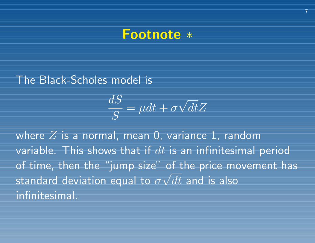
Footnote ∗

The Black-Scholes model is

dS

S= µdt + σ

√dtZ

where Z is a normal, mean 0, variance 1, random

variable. This shows that if dt is an infinitesimal period

of time, then the “jump size” of the price movement has

standard deviation equal to σ√

dt and is also

infinitesimal.

8

Historical EMH Tests

One of the strongest proponents of the EMH is Burton

Malkiel in the book ”Random Walk Down Wall Street.”

In his book Malkiel cites many tests of EMH e.g.:

• Fama and Blume (1966)

• Van Horne and Parker (1967)

• Jensen and Benington (1970)

9

All these studies conclude that no advantage can be

gained by Technical Analysis.

However, some studies, not cited in Malkiel, claim to

have shown that there is an edge to be had in certain

technical systems. For example:

• Brock, W., Lakonishock, J. and LeBaron, B. (1992)

proport that moving average and trading range breakout

trading shows consistent, positive results.

An excellent run-down of tests of the EMH can be found

10

in, “What do we know about the profitability of

Technical Analysis?” by Park and Irwin (2004) and

available on the internet for free.

11

Our Basic Test

Taking moment-to-moment in option pricing theory to

mean day-to-day, we first test the extent to which the

price of a stock tomorrow is up or down relative to today.

The test can be conducted on a restricted range of

stocks or dates.

We do this:

• a stock and a date are randomly selected compliant with

12

the restrictions

• the closing price of that stock on that date is noted,

and

• this price is compared with the closing price on the next

market day

• if they are the same, the sample is discarded; otherwise

the result is tabulated up or down

The statistic calculated is the probability p that a stock’s

price will be up tomorrow relative to today.

13

To generate confidence intervals for p, the samples are

batched 100 at a time. The batches are therefore

normally distributed. A run consists of 1,000 batches

typically. (Altogether then a run consists of 100,000

samples.)

Here is an example run:

NYSE, 1990 – 2008, 95.4% confidence interval (CI)

p = 49.91± .32

14

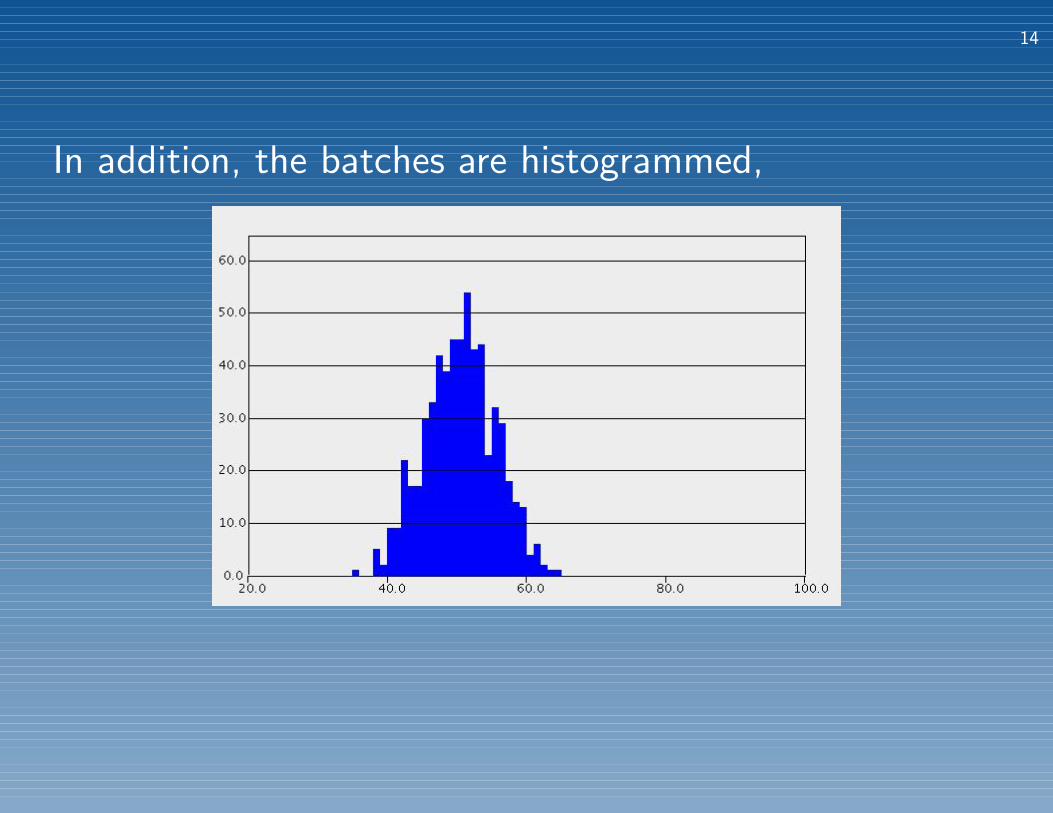
In addition, the batches are histogrammed,

15

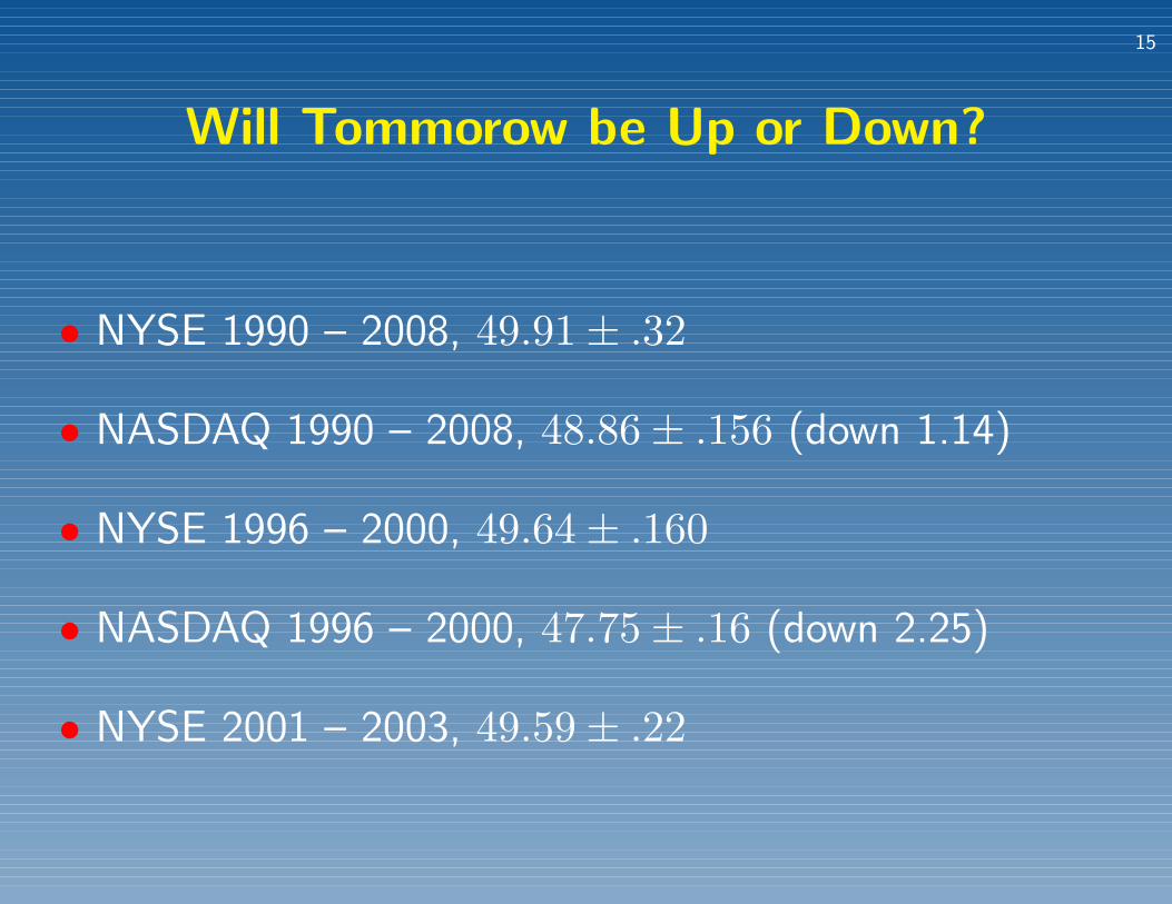
Will Tommorow be Up or Down?

• NYSE 1990 – 2008, 49.91± .32

• NASDAQ 1990 – 2008, 48.86± .156 (down 1.14)

• NYSE 1996 – 2000, 49.64± .160

• NASDAQ 1996 – 2000, 47.75± .16 (down 2.25)

• NYSE 2001 – 2003, 49.59± .22

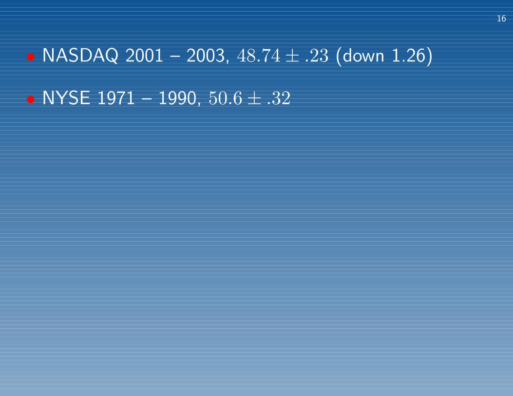
16

• NASDAQ 2001 – 2003, 48.74± .23 (down 1.26)

• NYSE 1971 – 1990, 50.6± .32

17

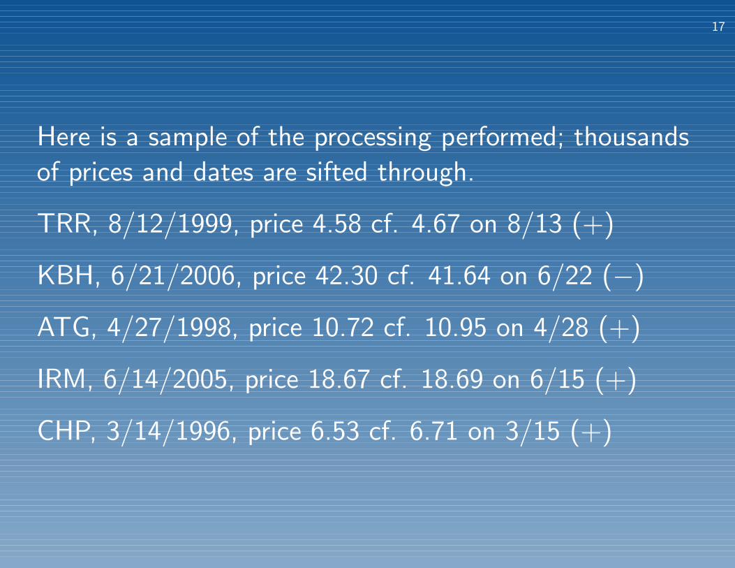
Here is a sample of the processing performed; thousands

of prices and dates are sifted through.

TRR, 8/12/1999, price 4.58 cf. 4.67 on 8/13 (+)

KBH, 6/21/2006, price 42.30 cf. 41.64 on 6/22 (−)

ATG, 4/27/1998, price 10.72 cf. 10.95 on 4/28 (+)

IRM, 6/14/2005, price 18.67 cf. 18.69 on 6/15 (+)

CHP, 3/14/1996, price 6.53 cf. 6.71 on 3/15 (+)

18

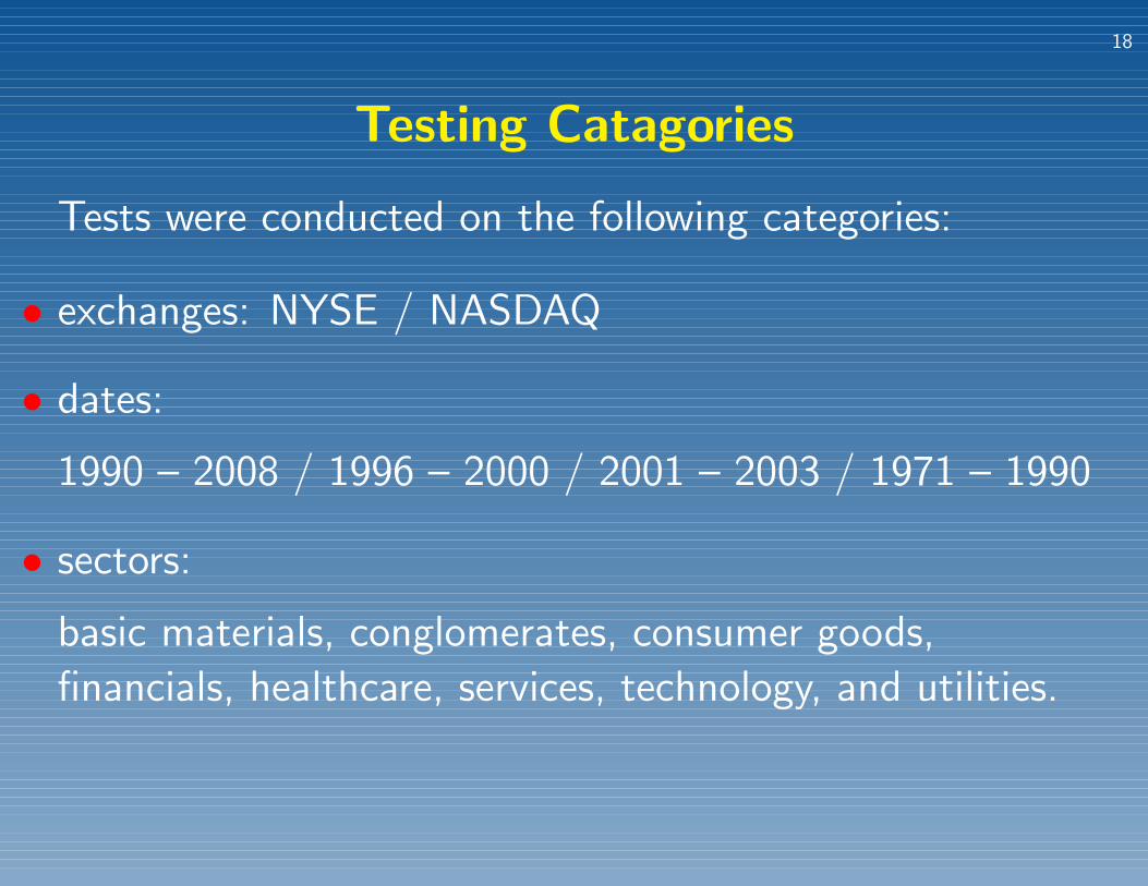
Testing Catagories

Tests were conducted on the following categories:

• exchanges: NYSE / NASDAQ

• dates:

1990 – 2008 / 1996 – 2000 / 2001 – 2003 / 1971 – 1990

• sectors:

basic materials, conglomerates, consumer goods,

financials, healthcare, services, technology, and utilities.

19

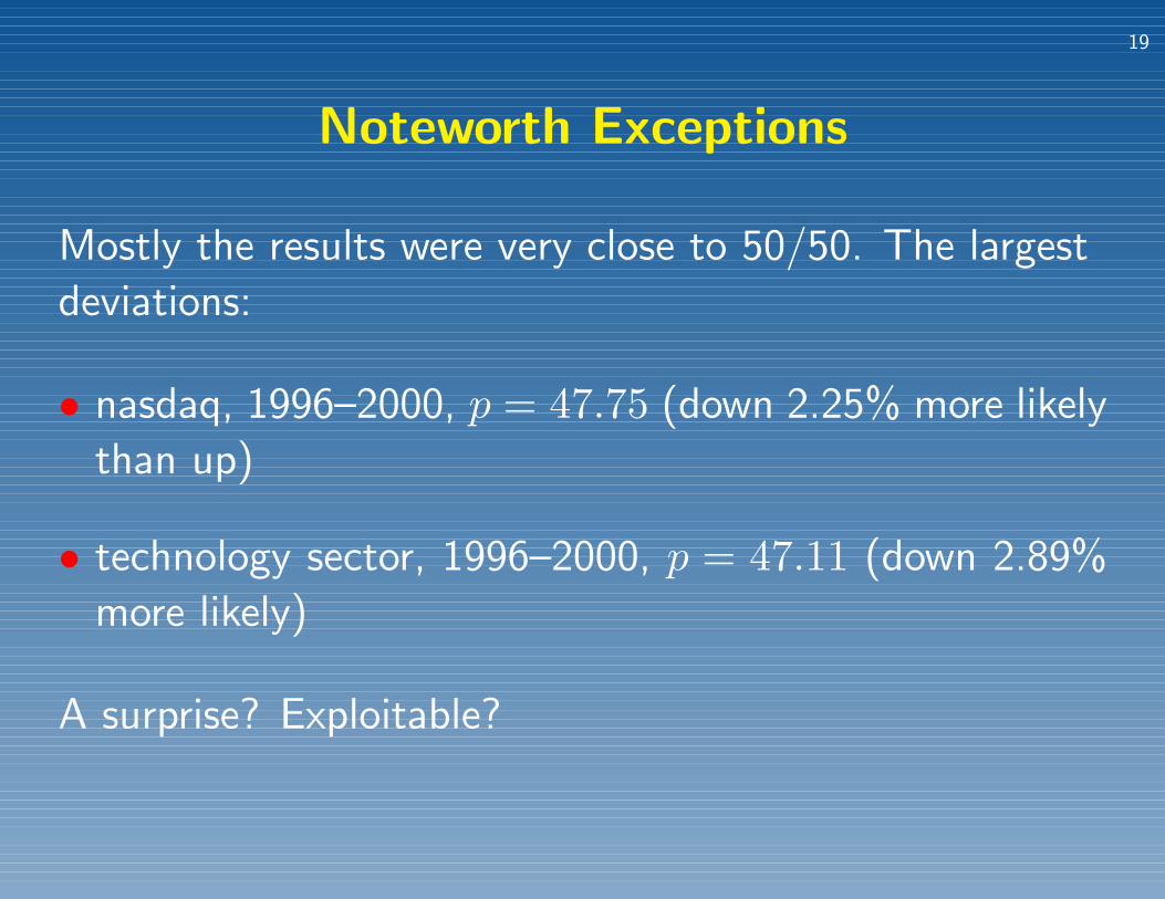
Noteworth Exceptions

Mostly the results were very close to 50/50. The largest

deviations:

• nasdaq, 1996–2000, p = 47.75 (down 2.25% more likely

than up)

• technology sector, 1996–2000, p = 47.11 (down 2.89%

more likely)

A surprise? Exploitable?

20

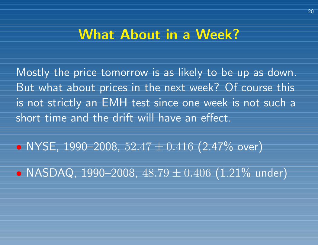
What About in a Week?

Mostly the price tomorrow is as likely to be up as down.

But what about prices in the next week? Of course this

is not strictly an EMH test since one week is not such a

short time and the drift will have an effect.

• NYSE, 1990–2008, 52.47± 0.416 (2.47% over)

• NASDAQ, 1990–2008, 48.79± 0.406 (1.21% under)

21

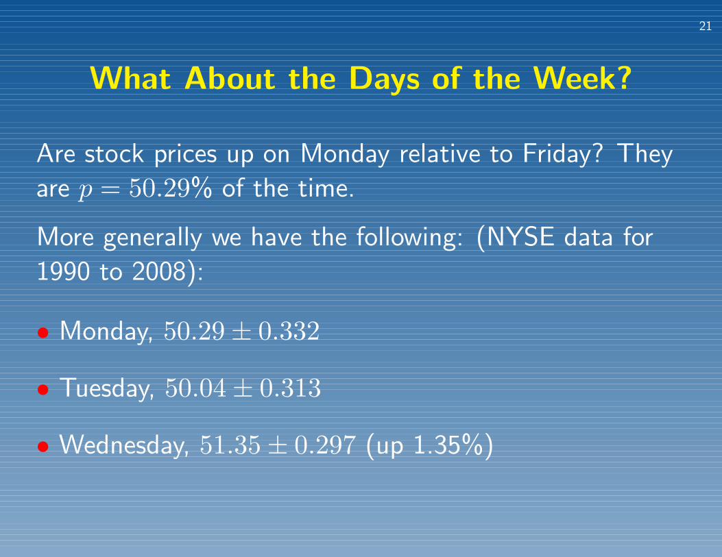
What About the Days of the Week?

Are stock prices up on Monday relative to Friday? They

are p = 50.29% of the time.

More generally we have the following: (NYSE data for

1990 to 2008):

• Monday, 50.29± 0.332

• Tuesday, 50.04± 0.313

• Wednesday, 51.35± 0.297 (up 1.35%)

22

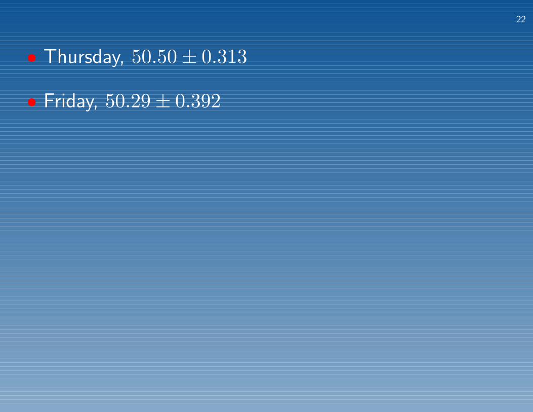
• Thursday, 50.50± 0.313

• Friday, 50.29± 0.392

23

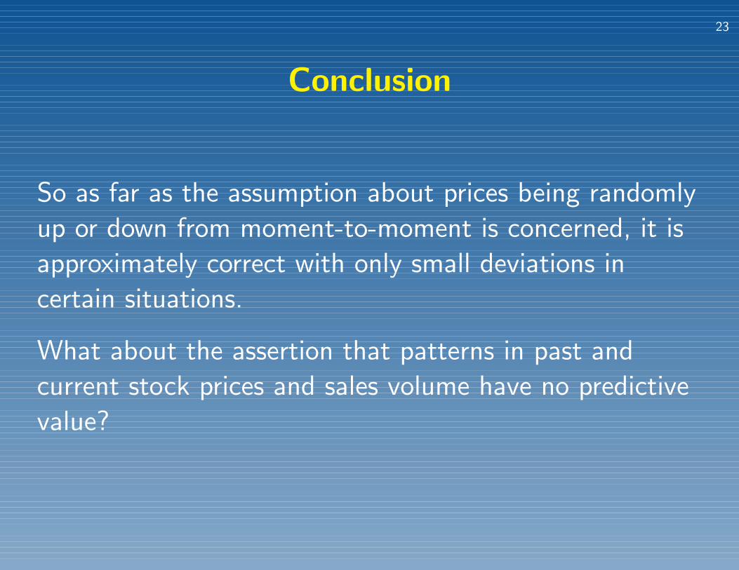
Conclusion

So as far as the assumption about prices being randomly

up or down from moment-to-moment is concerned, it is

approximately correct with only small deviations in

certain situations.

What about the assertion that patterns in past and

current stock prices and sales volume have no predictive

value?

24

Technical Indicators

The EMH implies that Technical Analysis is of no value,

all information available in charts is already incorporated

into the stock’s price; future price movement is due to

news.

Is it true?

25

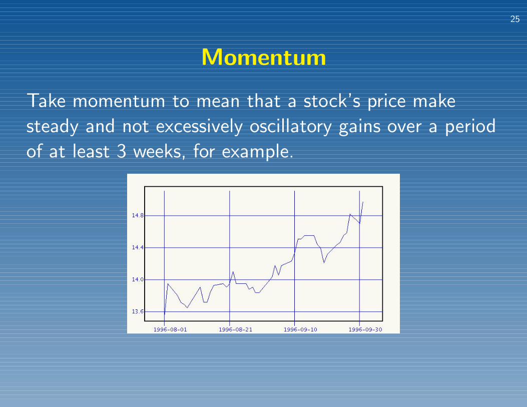
Momentum

Take momentum to mean that a stock’s price make

steady and not excessively oscillatory gains over a period

of at least 3 weeks, for example.

26

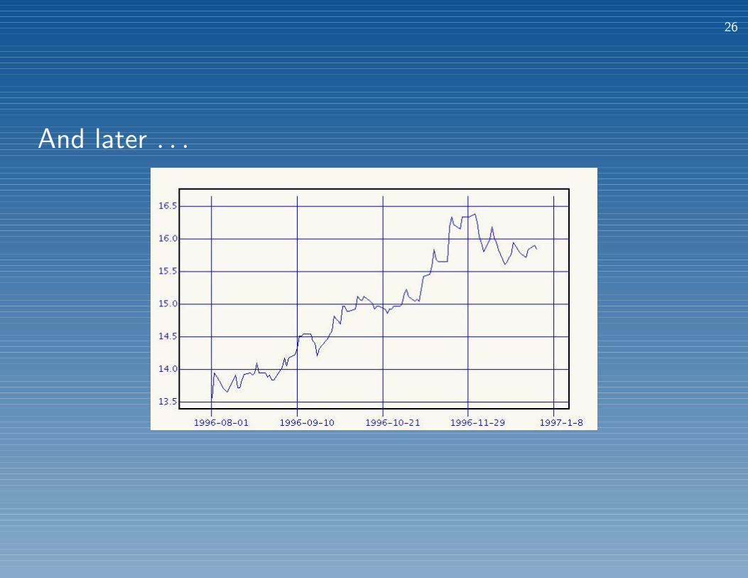
And later . . .

27

Do Stock Prices Have Momentum?

• NYSE, 1990–2008, gain 7cents/day over 20 days: up

tomorrow 50.9%

• NYSE, 1990–2008, gain 7cents/day over 45 days: up

tomorrow 52.2%

• NYSE, 1990–2008, gain 7cents/day over 45 days: up

next week 50.6%

28

Direction Movement Indicator (DMI)

OptionVue’s Steve Lenz suggests DMI generates a good

signal. “The amount by which today’s price is higher

than yesterday’s is dm+. Conversely, the amount by

which today’s price is below yesterday’s is (numerically)

dm-. Whichever is smallest on a given day is reset to 0.

The DMI indicator is the moving average of the

difference typically over 14 days. A signal is generated

when the 14 day dm+ crosses above the 14 day dm-.”

29

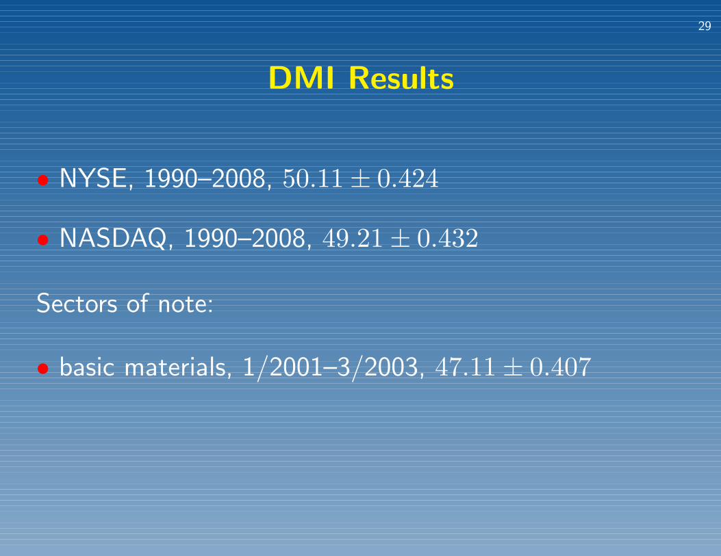
DMI Results

• NYSE, 1990–2008, 50.11± 0.424

• NASDAQ, 1990–2008, 49.21± 0.432

Sectors of note:

• basic materials, 1/2001–3/2003, 47.11± 0.407

30

The Hammer

“The Hammer is comprised of one candle identified by

the presence of a small body with a shadow at least two

times greater than the body. Found at the bottom of a

downtrend, this shows evidence that the bulls started to

step in. The color of the small body is not important but

a white candle has slightly more bullish implications than

the black body.”

31

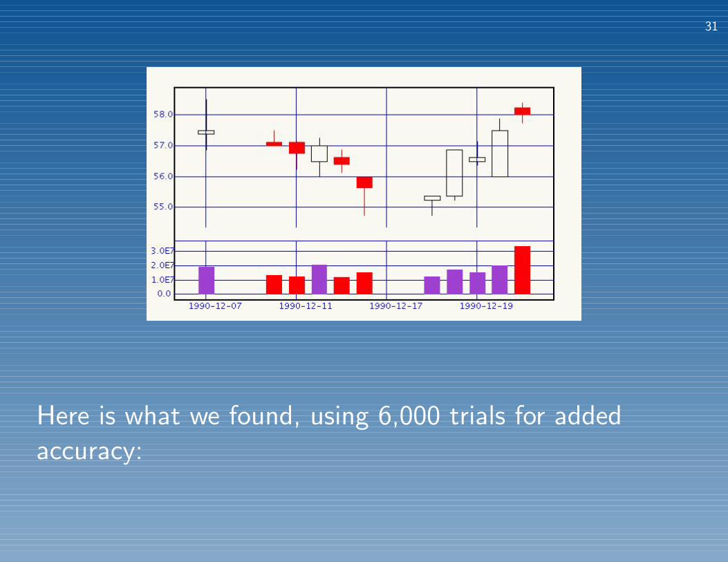
Here is what we found, using 6,000 trials for added

accuracy:

32

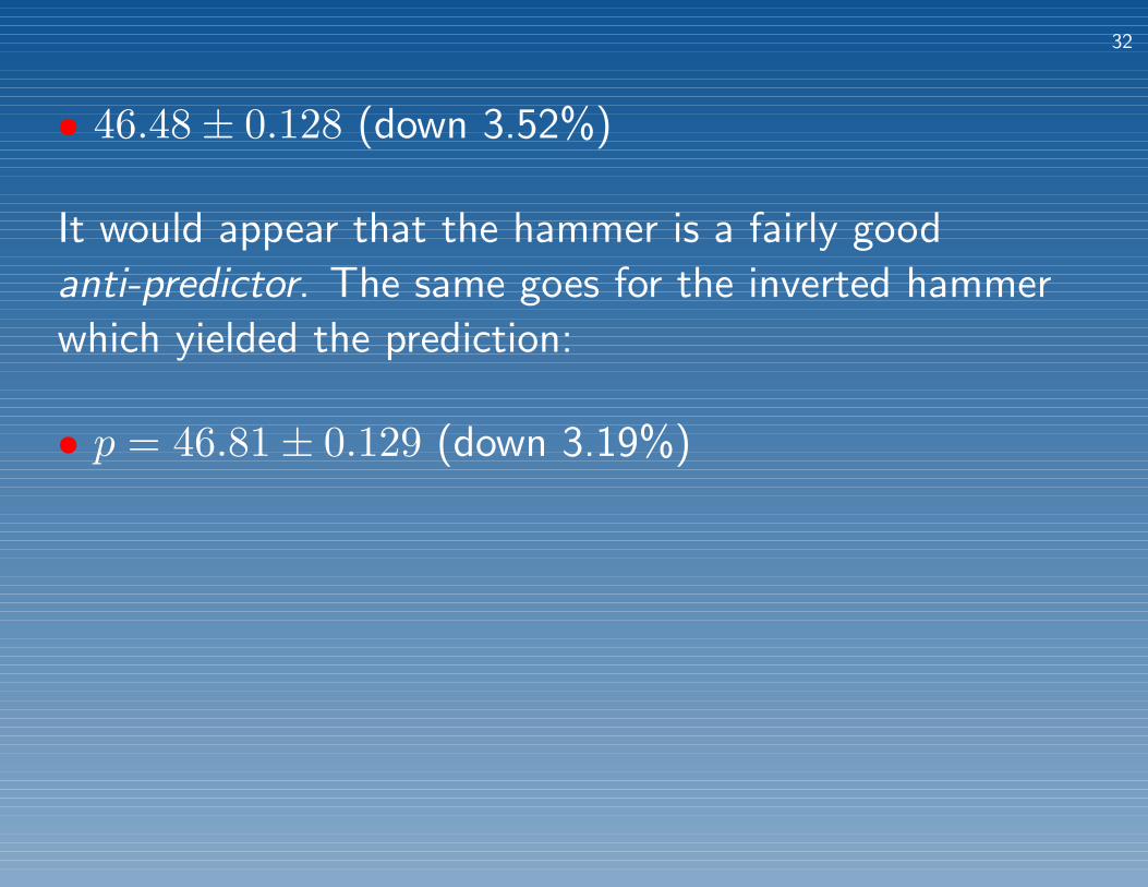
• 46.48± 0.128 (down 3.52%)

It would appear that the hammer is a fairly good

anti-predictor. The same goes for the inverted hammer

which yielded the prediction:

• p = 46.81± 0.129 (down 3.19%)

33

Two at a Time

I also tested some combinations of two at a time.

Suppose both dmi and momentum indicate the price will

rise.

• NYSE 1990–2008, 30 day gain of at least 3cents/day,

51.18± 0.407 (up 1.18%)

34

Moving Average Convergence/Divergence(MACD)

“MACD is the difference between a short term moving

average and a long term moving average. When the

short term exceeds the long term by a certain amount,

then then stock is overbought, the stock price is

predicted to fall. Conversely when the short term is less

than the the long term by more than a certain amount

then the stock is oversold, the price will rise.”

35

MACD Results

• NYSE 1990–2008, 12/26 day MA, 55.64± 0.414

• NASDAQ 1990–2008, 12/26 day MA, 52.80± 0.410

36

Recall we are testing whether or not the price tomorrow

is up relative to today if and when a signal is generated,

the data show that 55.6% of the time the stock price

agreed with the prediction when a MACD signal was

generated.

As pointed out at the beginning of the talk, this result

confirms that of Brock, Lakonishock, and LeBaron.

Can it be exploited ... ?

37

Some Recent Results

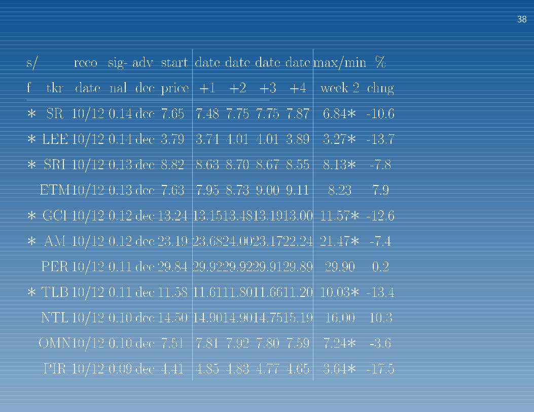
38

s/ reco sig- adv start date date date date max/min %

f tkr date nal dec price +1 +2 +3 +4 week 2 chng

∗ SR 10/12 0.14 dec 7.65 7.48 7.75 7.75 7.87 6.84∗ -10.6

∗ LEE 10/12 0.14 dec 3.79 3.74 4.01 4.01 3.89 3.27∗ -13.7

∗ SRI 10/12 0.13 dec 8.82 8.63 8.70 8.67 8.55 8.13∗ -7.8

ETM10/12 0.13 dec 7.63 7.95 8.73 9.00 9.11 8.23 7.9

∗ GCI 10/12 0.12 dec 13.24 13.1513.4813.1913.00 11.57∗ -12.6

∗ AM 10/12 0.12 dec 23.19 23.6824.0023.1722.24 21.47∗ -7.4

PER 10/12 0.11 dec 29.84 29.9229.9229.9129.89 29.90 0.2

∗ TLB 10/12 0.11 dec 11.58 11.6111.8011.6611.20 10.03∗ -13.4

NTL 10/12 0.10 dec 14.50 14.9014.9014.7515.19 16.00 10.3

OMN10/12 0.10 dec 7.51 7.81 7.92 7.80 7.59 7.24∗ -3.6

PIR 10/12 0.09 dec 4.41 4.85 4.83 4.77 4.65 3.64∗ -17.5

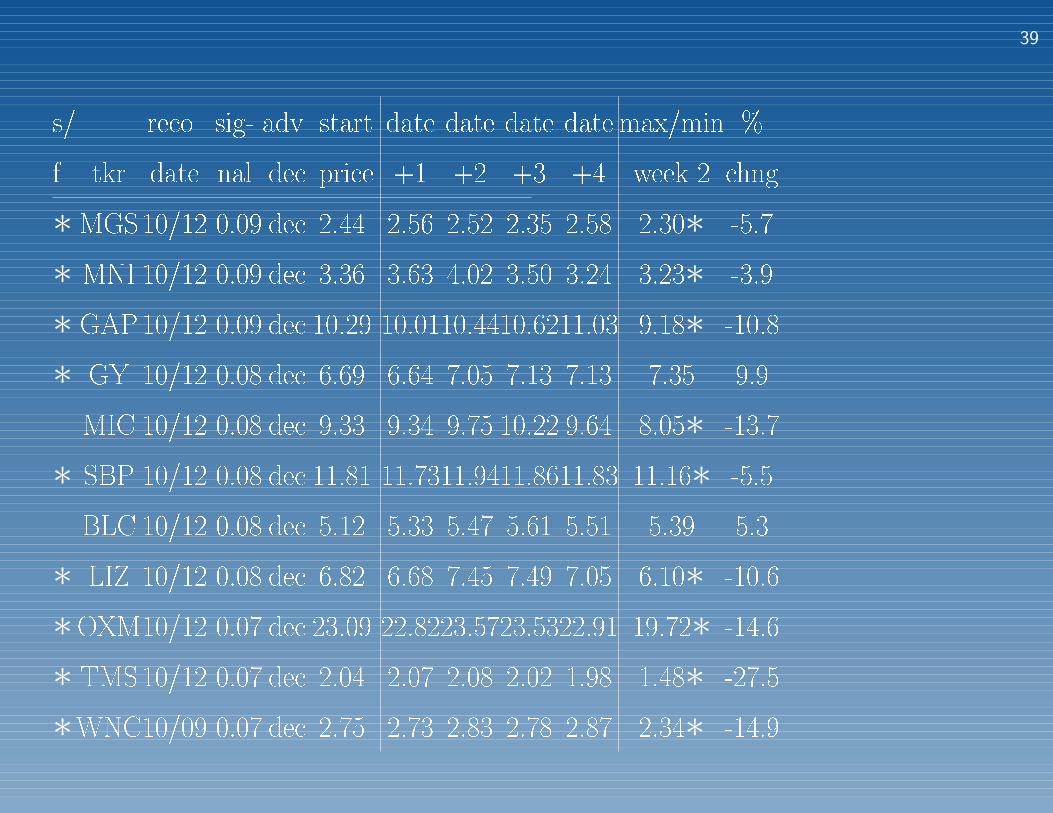
39

s/ reco sig- adv start date date date date max/min %

f tkr date nal dec price +1 +2 +3 +4 week 2 chng

∗MGS10/12 0.09 dec 2.44 2.56 2.52 2.35 2.58 2.30∗ -5.7

∗ MNI 10/12 0.09 dec 3.36 3.63 4.02 3.50 3.24 3.23∗ -3.9

∗ GAP10/12 0.09 dec 10.29 10.0110.4410.6211.03 9.18∗ -10.8

∗ GY 10/12 0.08 dec 6.69 6.64 7.05 7.13 7.13 7.35 9.9

MIC 10/12 0.08 dec 9.33 9.34 9.75 10.22 9.64 8.05∗ -13.7

∗ SBP 10/12 0.08 dec 11.81 11.7311.9411.8611.83 11.16∗ -5.5

BLC 10/12 0.08 dec 5.12 5.33 5.47 5.61 5.51 5.39 5.3

∗ LIZ 10/12 0.08 dec 6.82 6.68 7.45 7.49 7.05 6.10∗ -10.6

∗OXM10/12 0.07 dec 23.09 22.8223.5723.5322.91 19.72∗ -14.6

∗ TMS10/12 0.07 dec 2.04 2.07 2.08 2.02 1.98 1.48∗ -27.5

∗WNC10/09 0.07 dec 2.75 2.73 2.83 2.78 2.87 2.34∗ -14.9

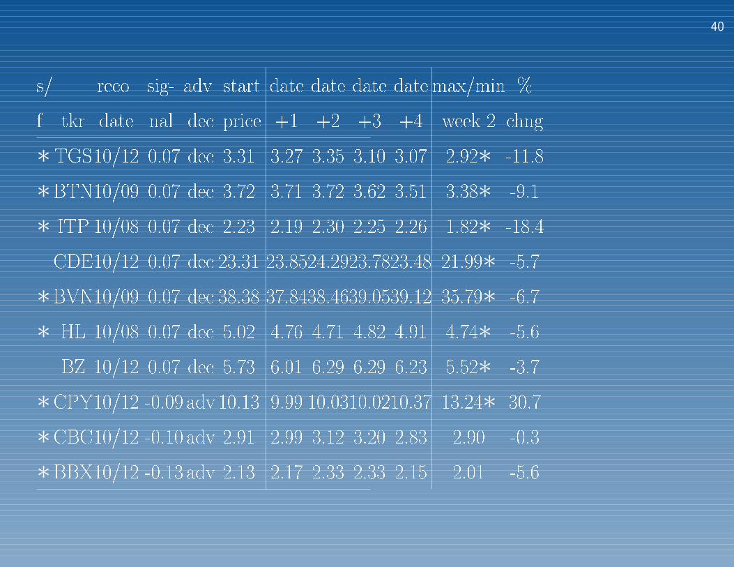
40

s/ reco sig- adv start date date date date max/min %

f tkr date nal dec price +1 +2 +3 +4 week 2 chng

∗TGS10/12 0.07 dec 3.31 3.27 3.35 3.10 3.07 2.92∗ -11.8

∗BTN10/09 0.07 dec 3.72 3.71 3.72 3.62 3.51 3.38∗ -9.1

∗ ITP 10/08 0.07 dec 2.23 2.19 2.30 2.25 2.26 1.82∗ -18.4

CDE10/12 0.07 dec 23.31 23.8524.2923.7823.48 21.99∗ -5.7

∗BVN10/09 0.07 dec 38.38 37.8438.4639.0539.12 35.79∗ -6.7

∗ HL 10/08 0.07 dec 5.02 4.76 4.71 4.82 4.91 4.74∗ -5.6

BZ 10/12 0.07 dec 5.73 6.01 6.29 6.29 6.23 5.52∗ -3.7

∗CPY10/12 -0.09 adv 10.13 9.99 10.0310.0210.37 13.24∗ 30.7

∗CBC10/12 -0.10 adv 2.91 2.99 3.12 3.20 2.83 2.90 -0.3

∗BBX10/12 -0.13 adv 2.13 2.17 2.33 2.33 2.15 2.01 -5.6

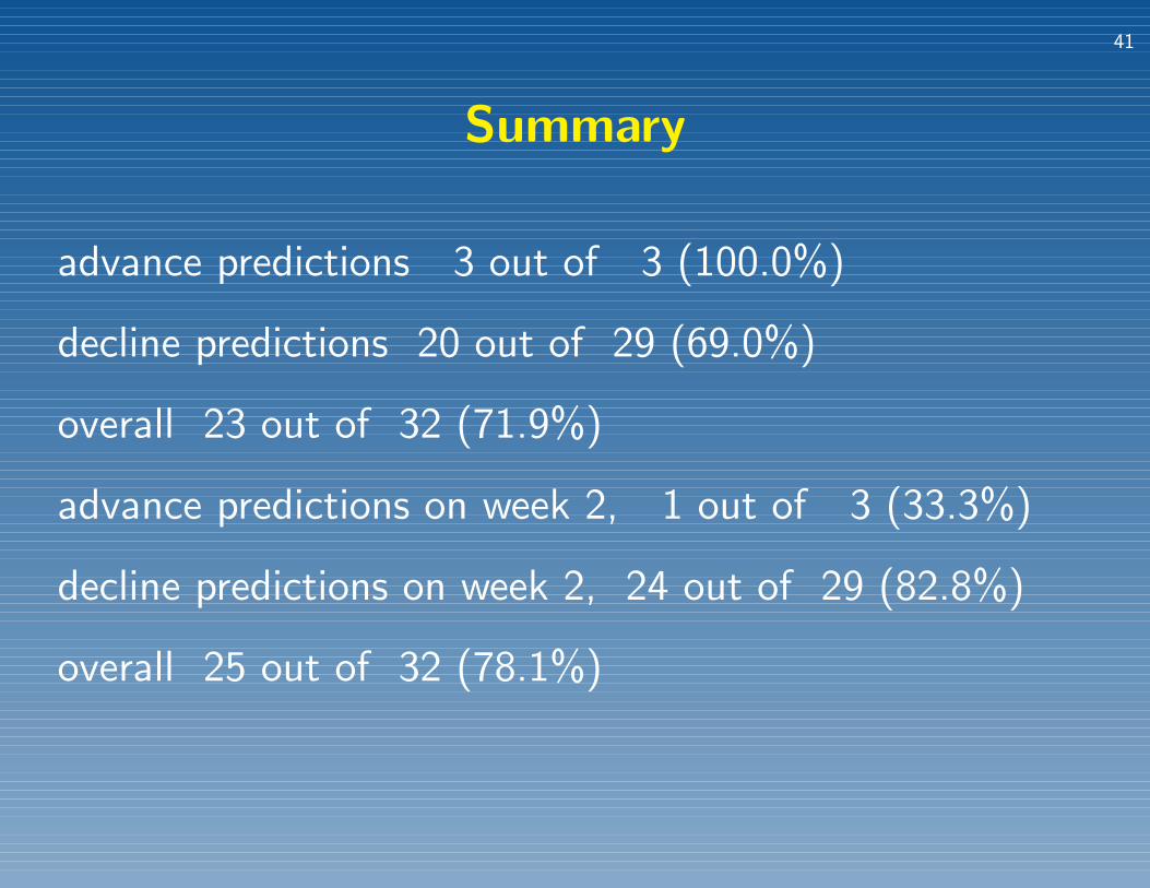
41

Summary

advance predictions 3 out of 3 (100.0%)

decline predictions 20 out of 29 (69.0%)

overall 23 out of 32 (71.9%)

advance predictions on week 2, 1 out of 3 (33.3%)

decline predictions on week 2, 24 out of 29 (82.8%)

overall 25 out of 32 (78.1%)

42

Over Aug/Sept/Oct

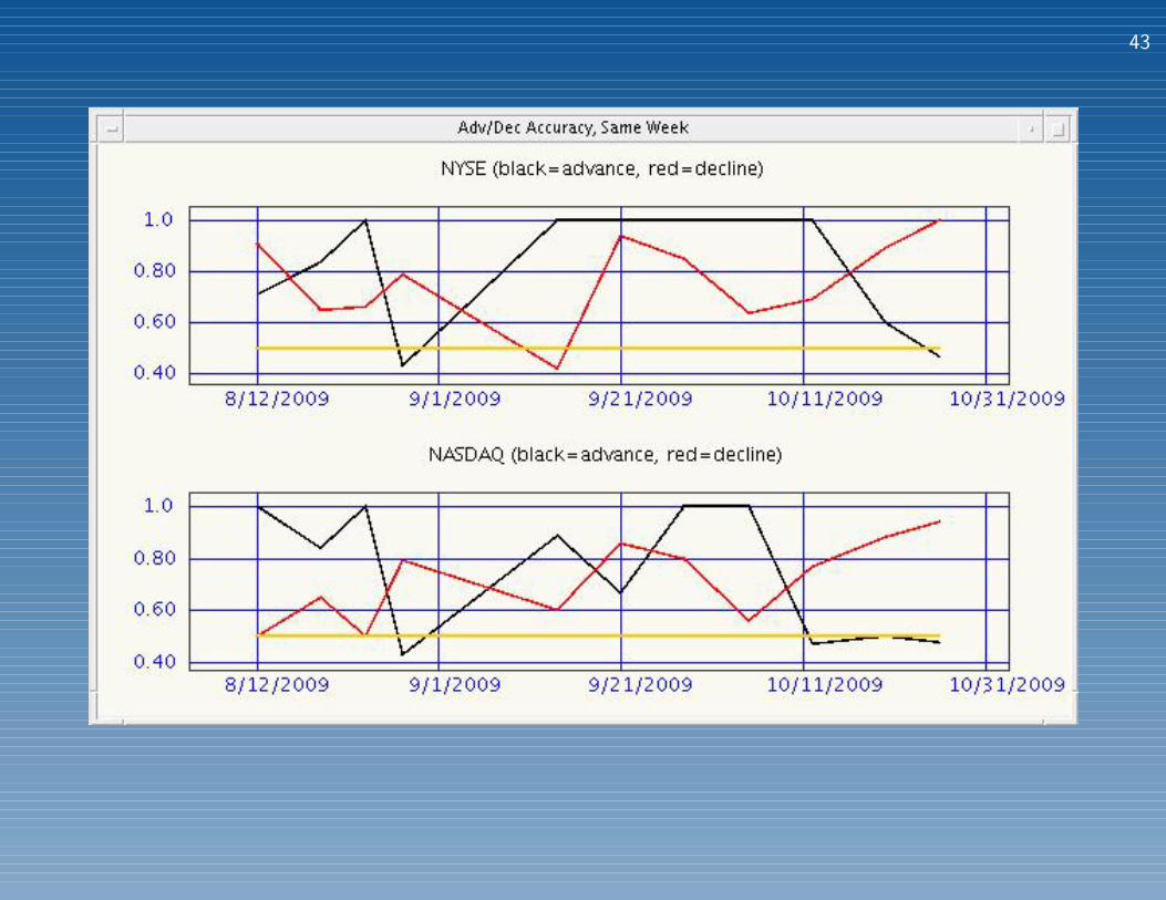
43