Testing the effectiveness of the French work-sharing

reform: a forecasting approach∗

Camille LogeayGerman Institute for Economic Research,

Berlin

clogeay@diw.de

Sven Schreiber†

Goethe-University Frankfurt

sschreiber@wiwi.uni-frankfurt.de

This revision: July 2004

Abstract

We analyze the macroeconomic impact of the French work-sharing reform

of 2000 (a reduction of standard working hours in combination with wage sub-

sidies). Using a vector error correction model (VECM) for several labor mar-

ket variables as well as inflation and output we produce out-of-sample forecasts

for 2000/2001. A comparison of these forecasts –which serve as a benchmark

simulation without structural shifts– to the realized values (with shifts) suggests

significant beneficial employment effects of the policy mix. Other shifts were

absent and thus cannot explain the outcome. Output, productivity, hourly labor

costs, and inflation are only transitorily affected or not at all.

JEL: E24, E27, C32

Keywords: unemployment, work-sharing, France, VECM, forecasting

1 Introduction

At the turn of the millennium, the French unemployment rate decreased by 2.2%-

points (1999-2001) after more than a decade with stubbornly high unemployment.

∗We wish to thank participants of the Berlin Econometrics Seminar, EALE, and Ecomod meetings aswell as Michael Funke, Bernard Salzmann, and an anonymous referee for helpful comments, and NathalieFourcade for help with the data. We remain responsible for any mistakes.

†Corresponding author, Dept. of Economics, Mertonstr. 17 (PF82), D-60054 Frankfurt, Germany;phone +49/69/798-28804, fax +49/69/798-28933.

1

The rest of the Eurozone experienced a decline as well, but the amount of 1.2%-points

was markedly lower (see table1 below for this and other basic data). An analogous

feature can be observed in employment figures: after growth rates below average in

1995-1998, France experienced above average growth rates from 1999 to 2002. The

rest of the Eurozone shared the tendency of the movement, but not quite its extent.

This development may partly be attributed to the above Eurozone-average real

GDP growth in France (3.1% p.a. for France against 2.5% p.a. for the rest of the Eu-

rozone in 1997-2001). However, another event that had an important influence on the

economic environment of France during this period was a “work-sharing” reform. A

brief summary of the complex institutional setting could read as follows: On the one

hand, the standard workweek was reduced from 39 to 35 hours, first on a voluntary

basis coupled with incentive schemes conditional on employment creation (Robien act

1996, Aubry I act 1998), then on a compulsory basis (Aubry II act 2000). On the other

hand the following alleviations were offered to firms: Greater managerial flexibility

w.r.t. working time allocation (Robien, Aubry I), payroll tax cuts through lower so-

cial security contributions for employers (in all acts), and a negotiated mid-term wage-

income growth restraint.

The explicit aim of this policy mix was to reduce unemployment levels. Thus it is

interesting to analyze if the reform had any noticeable effect or if it was just ordinary

economic growth that did the work. Also from the perspective of economic theory it is

still an unsettled issue whether a reduction of standard hours (alone) will lead to more

or less unemployment since in most models the outcome is in general ambiguous.

Earlier studies provided mixed results, see below, and a general consensus has not

been reached. Recent empirical assessments of other work-sharing reforms have not

been positive, see Hunt (1999) or Crepon and Kramarz (2002). But the respective

German and French/1982 reforms included persistent hourly wage hikes as income

compensation for workers and no alleviation for firms, such that the negative outcome

is perhaps not too surprising. However, the institutional environment of the recent

French reform was quite different which provides an interesting new perspective on

2

the issue of work-sharing.

The existing literature in the context of the recent French reform falls into roughly

three classes: First there were ex-ante simulations of several scenarios within macro

models (see e.g. DARES-BDF-OFCE 1998), second there is descriptive evidence (e.g.

DARES 2002), and finally micro data for selective samples of firms have been thor-

oughly analyzed (Bunel 2002, Passeron 2002). For those studies that allow drawing

conclusions with respect to employment effects, the results are mostly optimistic.

Our aim is to complement the literature by shedding some light on the macroe-

conomic consequences of the recent French work-sharing reform. To this end we

estimate an empirical system of labor market variables (as well as inflation and output)

using a vector error correction model (VECM) up to 1999. As there are two competing

possible break dates (namely 1999q4 and 2000q1, see section3 for detailed results),

we actually estimate two slightly different models. With these models we can pro-

duce forecasts for the subsequent period, acknowledging the fact that those forecasts

are based on the previous institutional regime. A comparison to actual observations

after the introduction of the 35h work-week allows us to pinpoint significant changes.

For both models we get very similar results; we find that unemployment was reduced

throughout the analyzed horizon at the cost of a transitory depression of total hours

worked reflecting a short-run rise of hourly labor costs. Labor costs and inflation re-

main somewhat higher than their forecasts, but not significantly so. Output is forecast

quite well in every period and in general seems unaffected by the break.

These results can be attributed to the work-sharing-cum-lower-costs reform be-

cause other forces that could have had an influence on the unemployment rate were

absent: For example, the labor supply grew at normal rates (see table1), if not faster

than usual. The coverage of active labor market policy actually declined somewhat

during our forecast period (Boulard and Lerais 2002), which makes our estimates even

slightly conservative. National accounts data show that other stimuli such as an ex-

pansionary fiscal policy did not occur, and not even ECB officials or other pro-Euro

economists claimed that the introduction of the Euro would fight unemployment; in-

3

stead they have always called for structural labor market reforms. (Also recall that the

Euro was adopted already in the beginning of 1999, not in 2000.) But even if these

arguments are disputed, our real output forecast turns out to be surprisingly accurate,

such that potentially stimulating business-cycle effects would be controlled for.

The rest of this contribution is structured as follows: In the next section we provide

a brief survey of the relevant literature, we describe some institutional details of the re-

form, and we discuss estimates and implications of existing studies. Section3 presents

the data and explains our model specification along with the resulting forecasts. The

final section summarizes the main findings.

[Tables1 and2 about here]

2 Theory, institutions, and existing evaluations

2.1 A glimpse at the recent work-sharing debate

Economists are usually very critical about work-sharing due to the “lump-of-labor”

fallacy, i.e. the assumption of a fixed labor input volume that is often implicitly made

in public debates on the issue (Layard, Nickell, and Jackman 1991, Snower 1997).

But most of the theoretical studies yield ambiguous predictions depending on what the

precise model or parameter values are.

For example, in the reference model of Calmfors and Hoel (1988) even the most

skeptical model variant predicts a definitely negative response of output and employ-

ment only if the overtime premium is constant. If a progressive premium system is

allowed instead, the response becomes uncertain. The predictions of the model by

FitzRoy, Funke, and Nolan (2002) are more optimistic, although it coincides with the

conclusions in Marimon and Zilibotti (2000), where the possible employment creation

would lower firms’ profits. In contrast to that, a possible Pareto improvement is found

in the matching models by Rocheteau (2002) and by Ortega (2003), where lower stan-

dard hours may offer a firm more flexibility to react to demand shocks.

4

On the empirical side, the results are also mixed. Crepon and Kramarz (2002) ana-

lyze the reduction of 40 to 39 hours in 1982 for France. At that time full wage income

compensation without reorganizational possibilities were the norm. Not surprisingly,

they find a negative effect on employment. In Hunt (1999), a similar work-sharing

reform without wage moderation is analyzed for West Germany in 1984-1994. De-

pending on the data set and method used she finds mostly insignificant coefficients of

both signs. On the other hand, after conditioning on wages Franz and Konig (1986)

find a positive partial effect of normal hours reduction on employment for West Ger-

many (p. S241), although it is not mainly a study about work-sharing.1

In contrast to former experiences, the reforms that recently took place in France

implied working-time reduction against tax cuts and subsequent wage growth restraint.

This policy mix therefore may have been more effective than earlier work-sharing

attempts.

2.2 The institutional background in France

The shortening of the standard work-week was implemented in several stages. A first

act to reduce working-time (named Robien) was passed in June 1996. This voluntary

measure had only very little impact, covering only 0.3m employees between June 1996

and June 1998 (Passeron 2002).

The main reform project was implemented in two stages. First the Robien act

was replaced by the Aubry I act in June 1998 which lowered the legally standard

work-week to 35 hours. (Martine Aubry was the minister of labor between June 1997

and October 2000.) However, while it became effective for firms with more than 20

employees on January 1st, 2000, smaller firms would not be affected until January

2002. Additionally an incentive scheme was introduced to promote a quickereffective

work-week reduction. The most important exception in this legislation was the civil1This list of empirical studies is of course not complete, but conveys the status quo of the research,

namely that evidence is diverse, and that a consensus has not been reached. Further references are given inOrtega (2003), Marimon and Zilibotti (2000), and Hunt (1999). The link between actual hours and legalhours was studied for the U.S. by Trejo (1991) and Costa (2000), arguing that work-sharing is irrelevantif firms and workers negotiate a constant compensation/workload-package. They find non-neutrality oflower working hours, whereas in Trejo (2001) irrelevance of work-sharing cannot be rejected.

5

service (but not state-owned firms). There were about 16m employees potentially

affected by this reform (DARES 2002), of which about one third worked in small

firms. (The overall number of employees in France in 2001 was about 22m people.)

The Aubry I incentive scheme provided reductions of social security contributions

for firms that effectively reduced the work-week and guaranteed a certain level of

employment. A useful source for details is Passeron (2002). Among the firms with a

work-week reduction up to the end of 2001, 58% participated in the Aubry I incentive

scheme (this covers 28% of all workers that had their working time reduced).

The second stage (Aubry II, passed in December 1999/January 2000) confirmed

the 39 to 35 hours transition and instated a system of structural aids. For bigger firms

the Aubry I scheme was being phased out, whereas for smaller firms the end date is

2002. The structural aids depend on wage levels; the average tax reduction per year

and employee was EUR 1067 (Passeron 2002); it was not conditional on guaranteed

employment levels anymore. Furthermore the flexibility of varying weekly hours over

the course of a year was increased. For a transition period of one year, the overtime

premium for the first four hours was reduced from 25% to 10% (the next four hours re-

mained subject to a 25% premium and hours beyond that must be paid at 150%). This

working-time reduction was mostly accompanied by an initial wage income compen-

sation (Pham 2002). For example, in 2000 98% of all employees covered by Aubry II

enjoyed a full wage compensation; however, 1/3 had to accept a wage stagnancy and

14% a wage growth moderation for the following one to three years.

Finally it should be noted that in some sense the work-sharing experience is already

history, because right after its election in early 2002 the new center-right government

started to reverse the reform.

2.3 Previous evaluations

Apart from the already mentioned descriptive evidence in DARES (2002), the macroe-

conomic studies for France were based on ex-ante simulations e.g. within the macro

models of the OFCE institute, the central bank (BdF), and the ministry of finance

6

(MINEFI). For a survey see Conseil Superieur de l’emploi, des revenus et des couts

(1998), DARES-BDF-OFCE (1998), or Commissariat General du Plan (2001). De-

pending on the various assumptions the assessment of the employment effects range

from optimistic (up to 700,000 additional jobs in the simulations of the OFCE and

of the BdF) to more sceptical (between 200 and 300,000 according to MINEFI, even

negative if a blockade between unions and employers is assumed).

The existing microeconomic studies (based on observed data) use samples of firms

with specific characteristics, apparently due to data limitations. Passeron (2002) for

example only analyzes firms in the Aubry I scheme. He concludes that the employ-

ment gain induced by the work-week reduction is between 6 and 7.5%. (Effects where

firms become eligible for subsidies without having beeninducedto meet the crite-

ria are supposedly not included in those numbers.) The resulting productivity gain

effect in his study is 4% which is a little more than what is often assumed on theoret-

ical grounds. According to Passeron the government subsidies decreased total labor

costs of the Aubry I firms by 4%. In addition to that, Passeron estimates a beneficial

“anti-seniority” effect of 1%, because newly hired workers are cheaper relative to their

productivity. Wage moderation is seen as 0.8%, such that altogether the work-week

reduction was approximately cost-neutral over the horizon until 2002. This study is

not representative for aggregates, and even the sign of the bias is ambiguous: Firms

that waited until 2000 to reduce their work-week receive less subsidies but also have

less restructuring costs. Another study for selected firms is Bunel (2002), who uses a

special data set (“Passages”) to compare all firms that reduced theireffectiveweekly

working time to 35 hours.

The existing macro evidence is only for scenarios, and it is not clear what the

selective micro studies imply for the aggregate level. An empirical macro analysis

therefore seems useful, and we now turn to it.

7

3 Empirical methods and results

3.1 Variables and data

In the context of imperfect competition, prices and wages are set simultaneously by

economic agents, see e.g. Layard, Nickell, and Jackman (1991), where the unemploy-

ment rate gives some feedback to the system. Therefore we require the following

variables: wages, prices, an employment measure, real output, and the unemployment

rate.

For wages there are basically three possibilities: 1. Total compensation including

social security contributions paid by employers, which represents the total cost of a

labor unit; 2. “gross” wages that include only social security contributions and taxes

paid by the worker herself; 3. net wages without taxes or contributions. For price

setting and the labor demand total compensation is clearly the appropriate variable.

For wage setting the level of net wages could also be relevant, but we restrict ourselves

to the total compensation measure, not least because net wages is a time series which

is difficult to obtain.

Prices: For labor demand and price setting it is the GDP deflator which is impor-

tant, while adding the consumer price index (CPI) would make sense for wage setting

analysis. Here we chose to include only the GDP deflator. Note that both price indices

display roughly the same development (not shown), such that the exclusion of the CPI

is not problematic.

Employment can be the labor volume (in hours) or the number of employed people,

where average working time links the two concepts. As the hours worked per person

is a central variable for the present study we include both employment measures. For

real output it is natural to choose real GDP, and the chosen unemployment rate is the

one according to ILO definitions.

W.r.t. the selected variable set it might be argued that potentially important vari-

ables are missing. Apart from the price/tax wedge and import prices, there are many

possible extensions. For example capital user costs may play a significant role as part

8

of marginal costs, and labor demand could also depend on the sectoral composition of

output. However, in this paper we do not follow up on these issues because our aim is

to work with a manageable labor market model. By analyzing the described data set

we have tried to follow a pragmatic middle-of-the-road approach.

The data are from the following sources: OECD, the French statistical office (IN-

SEE), and the statistical department of the French labor ministry (DARES); all series

are seasonally adjusted. The variable names, a survey of the sources and calculation

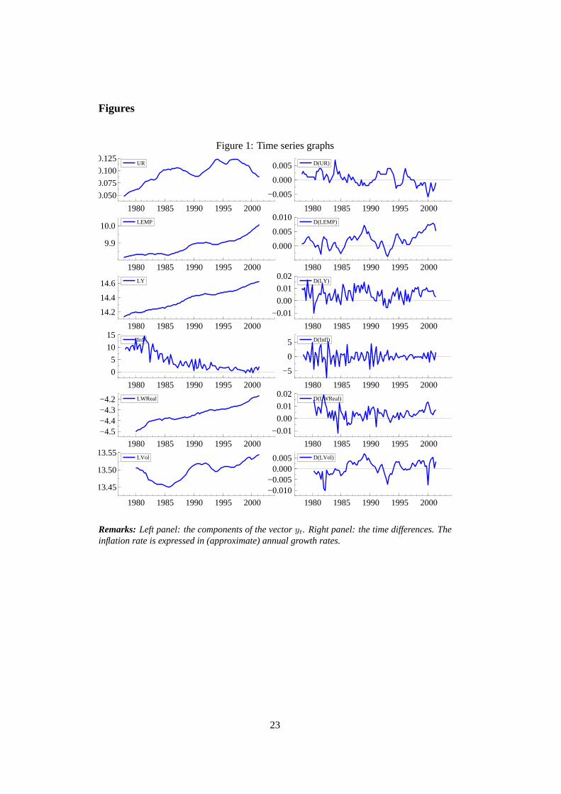
methods are given in table3. We present the analyzed time series in figure1 with some

anticipated transformations:LWRealt = LWt − LPYt will denote the hourly real

wage, andInflt = ∆LPYt(∗400) is essentially the first difference of the log price

level, i.e. the inflation rate.

Our general sample choice is determined by two facts: Data on hours worked are

only available from 1980 on, and it turns out that there is instability in the unemploy-

ment rate equation already towards the end of 1999, see the system analysis below

for more details. Thus the estimation period is set to 1980q1-1999q3, where the first

observations will be used as starting values for the necessary lagged regressors.

[Table3 about here]

[Figure1 about here]

3.2 Preliminary univariate data analysis

Obviously the inflation rate displays a very persistent behavior, such that using the

price level in the model would be difficult. But the inflation rate itself can well be in-

cluded as an integrated series (I(1)) in the multivariate system. Instead of the nominal

wage we therefore include the real wage “LWReal” (≡ LW − LPY ) in the system.

The variable vector is thus given by:

yt = (URt, LEMPt, LYt, Inflt, LWRealt, LV olt)′ (1)

The results of standard unit root tests are shown in table4. For all series the null

9

hypothesis of a unit root cannot be rejected, with the possible exception of the labor

volume. This does not pose any problemsper se, but another test in the system context

would still be interesting (see below).

[Table4 about here]

Before moving to the system analysis we perform a simple univariate forecast

of unemployment after the reduction of standard hours. Here we apply the standard

ARIMA model for the sample 1978q2-1999q3. We impose the unit root restriction

and after eliminating insignificant terms arrive at an ARIMA(3,1,2) specification. The

forecasts derived from this model beyond 1999q3 are displayed in figure2 along with

the forecast error confidence bands and the actually observed development. The devel-

opment of UR is clearly overestimated; actually, this model treats the unemployment

rate more or less as a random walk and thus simply sets the forecast close to the last

observed value. This automatically raises the question whether the information con-

tained in other variables enables us to produce better forecasts, or if the forecast failure

is due to a policy-induced structural break.

[Figure2 about here]

3.3 The multivariate forecasting model

Our statistical framework is the vector autoregressive model (VAR) with Gaussian

innovations that is widely used in empirical macroeconomics.2 We combine then = 6

variables in the column vectoryt for t = 1, ..., T , where in our caseT refers to 1999q3

or 1999q4, depending on the model variant, see below. Then the VAR has the following

shape:

yt =K∑

k=1

Φkyt−k + τt + µ + εt (2)

2For a textbook treatment see Lutkepohl (1991), and for the theory of a VAR with cointegration Jo-hansen (1995). The reported results were computed mainly with PcGive 10, see Doornik and Hendry(2001), with the exception of the Bartlett correction of the rank test which was performed with the pro-gram for RATS mentioned in Johansen (2002).

10

As deterministics a constantµ and a linear trend (serving as a proxy for technical

progress etc., with coefficientτ ) are allowed. After the appropriate reparametrization

the following vector error correction model (VECM) is obtained:

∆yt = Πyt−1 +K−1∑k=1

Γk∆yt−k + τt + µ + εt (3)

We adopt the conventional denomination for the matrix of the cointegration vec-

tors,β, and the matrix of adjustment coefficients,α, both of dimensionn × r for a

given cointegration rankr, such thatΠ = αβ′. The linear trend can only appear in the

cointegrating relations, i.e. we imposeτ = αρ′ (ρ freely varying).

First a choice about the number of lags in the VAR needs to be made. We use a

maximum of six lags, as this already means estimating 36+2 parameters in each equa-

tion. The Schwartz and HQ information criteria suggestK = 2, only the (inconsistent)

Akaike criterion choosesK = 6. However, because of remaining residual autocorre-

lation with two lags we are led to a choice ofK = 3. A single outlier in 1984q1

(especially in the unemployment equation) distorts the otherwise Gaussian properties

of the innovations, such that we include a restricted impulse dummy for that observa-

tion.3 Then the residual diagnostics are fully satisfactory, see table5.

[Table5 about here]

The rank of the matrixΠ is an important property of the system, although it is not

as crucial for forecasts as it would be for other analyses. We apply the well-known

Johansen procedure accounting for a restricted trend, see table6. Johansen (1995)

shows that this test procedure is unbiased if the rank tests are interpreted as a sequence,

starting from rank zero and stopping at the first insignificant test statistic. At first sight

the standard trace test statistics (in the third column) are all significant, and thus the

conclusion would be a (trend) stationary VAR without any unit roots in the system.

Apart from the fact that this would contradict the univariate unit root test evidence, it

3“Restricted” means that the impulse dummyi84q1t({. . . , 0, 0, 1, 0, 0, . . .}) is only allowed in thelevels of the data and not in the differences. This is achieved by includingi84q1t in the cointegrationspace and its difference∆i84q1t unrestrictedly in the VAR.

11

would be a highly unusual finding for macroeconomic time series.

However, the rank test is substantially oversized in small samples (i.e. it rejects

too often although the null hypothesis is true), and thus this nominal result may be

exaggerated. Fortunately, there exists a novel method to investigate this suspicion.

Following the Bartlett correction principle, Johansen (2002) develops a correction fac-

tor w.r.t. the rank test statistic. The idea is to find the expected value of the test statistic

for given models in small samples, compare that to the asymptotic value and derive

the corresponding correcting factor. It is obvious that this factor depends on nuisance

parameters that are asymptotically (and hence for the standard test setup) irrelevant.

The factor is applied to the measured test statistic and thereby the bias of the test is

decreased. Simulation studies show a beneficial effect.

In order to calculate the Bartlett corrections for the last four null hypotheses, we

estimated the VAR four times with the respective rank under the null to obtain the

necessary estimates of the parameter matrices. These were entered into the program of

Johansen (2002); the lag length is still fixed atK = 3. The results of this procedure are

provided in the last column of table6, and the test conclusions change considerably:

We have to stop atH0 : r = 4 when interpreting the sequence of corrected trace

tests, as this is the first non-rejected hypothesis. This choice implies thatn − r =

2 independent stochastic trends drive the system which is a reasonable property of

such a model. The results are not entirely straightforward because of the fact that –

viewed in isolation–H0 : r = 5 is also rejected. However, this is irrelevant for the

appropriate testing strategy of the Johansen procedure as explained before. Unreported

evidence about the estimated characteristic roots of the system also supports the choice

of exactly two unit roots. Therefore we proceeded with an imposed cointegration rank

of r = 4.

[Table6 about here]

It is beyond the scope of this paper to provide a structural analysis of the French

labor market. This aspect and the relatively high cointegration rank induced us to

refrain from an economic identification of the cointegrating relationships. However,

12

we checked that no harmful normalizations were used, e.g. no zero parameters were

normalized to unity.

We can now investigate a number of hypotheses within the cointegrated VAR:

First we return to the trend stationarity of the (log) labor volume. We test this as the

hypothesis that LVol alone is one of the components of the cointegration space. The LR

test of this restriction cannot reject, withχ2(2) = 3.76, p = 0.15. A second interesting

question is whether the linear trend is actually needed in the cointegrating relations.

The corresponding exclusion is clearly rejected (χ2(4) = 32.1, p = 0.00), so the trend

is essential for an adequate model. Finally, note that output does not adjust to any

equilibrium deviations (tested as a zero row in theα matrix,χ2(4) = 3.56, p = 0.47),

and is thus weakly exogenous for the long-run parameters. This partly explains why

we find that output is mostly unaffected by the structural break, see below.

3.4 Stability of the model and choice of breakpoint

The final check of the model is about its stability. Especially for our purposes a sta-

ble specification in the estimation period is obviously a desirable feature because an

unstable model would not yield meaningful forecasts.

Several recursively estimated test statistics indicate that parameter stability for the

described sample up to 1999q3 clearly holds, see figures3 through5. This means

that the quantitative impact of the previous reforms –Robien and Aubry I as described

before– was small and could easily be subsumed under the error term.

[Figures3, 4, and5 about here]

However, based on thea priori information about the beginning of the reform

we originally conjectured that any potential structural break should have happened

in 2000q1. But when we add the observation 1999q4 to the estimation period, there

is clear-cut evidence for instability at least in the unemployment equation (see figure

6), reflecting an unusual decline of the unemployment rate. As the coming reform

was publicly known in the end of 1999, this suggests that announcement effects were

13

already at work; the favorable product demand environment during that time probably

helped, too.

[Figure6 about here]

Given these findings, our strategy for the forecast test is to check both breakpoints

1999q4 and 2000q1 in the following way: For 1999q4, we simply estimate the model

until T = 1999q3 as described before and start our system forecast immediately af-

terwards. For the 2000q1 break date variant, we extend the estimation period until

T = 1999q4, but introduce an impulse dummy for the last observation to account for

the significant stability failure documented in figure6. (This impulse dummy is not

restricted to the cointegration space.) Note that the second variant is quite conserva-

tive in the sense thatno movements before 2000q1 are attributed to the work- sharing

reform.

Before we apply the forecasting model, note also that several robustness analyses

were done in the course of preparing this paper, varying both the number of lags, the

cointegration rank, and applying several model reduction strategies. The forecasts on

which our interest is centered were always very similar.

3.5 Forecasts and reality

Now we are in the position to answer the central question of this study, namely if the

policy of reducing standard hours in combination with wage subsidies had a significant

influence on the unemployment rate and other variables. To this end we compare the

observeddevelopment of the vectoryt until 2001q2 (i.e.yT+h, h = 1...H) and the

corresponding dynamic forecastsyfT+h = ET (yT+h), which are conditional on sam-

ple information up toT . These are computed recursively using the estimated VECM

coefficient matrices. For the first variant we haveT = 1999q3 andH = 7, whereas

the second variant usesT = 1999q4 andH = 6 (with an impulse dummy in 1999q4).

Our approach is related to the test of Box and Tiao (1976) which however is about

the joint significance of the forecast errors; a more detailed interpretation is possible

14

by considering the forecast errors separately. (The variance formulae for the entire

sequence of forecast errors can also be found in Clements and Hendry (1998).)

In line with our strategy of considering both 1999q3 and 1999q4 as potential break-

points, we present two sets of corresponding graphs in figures7 and8. There are some

quite interesting results to be pointed out:

[Figures7 and8 about here]

• The forecast of the unemployment rate (UR) falls slightly, but its confidence

bands drift apart quickly and become extremely large.In spite of thisthe ob-

served development of unemployment issignificantlylower than the forecast.

• Consequently, the employment development (LEMP) is consistently underesti-

mated. At the end of the forecast horizon the discrepancy of the forecast w.r.t.

reality constitutes about 0.5 million additional employed workers.

• The real output (LY) is forecast surprisingly well, so in this sense no extraordi-

nary goods market developments were responsible for the fall of the unemploy-

ment rate.

• There is nothing important to be seen in the inflation path, especially no dramatic

rise because of rising labor costs. However, the reliability of the forecast is very

low, given the extremely wide confidence bands stretching far into the negative

range.

• W.r.t. real hourly labor costs (LWReal) there is an unpredicted increase in the

beginning despite the paid subsidies. (The maximal difference between reality

and forecast is about 2%.) This is not surprising since an initial income com-

pensation had been negotiated which represents a short-run hourly wage hike.

However, this is gradually eliminated by subsequent wage growth restraint.

• Finally we observe a quite drastic slump of the labor volume (LVol) especially

in 2000q1, although this is slowly offset in the following quarters. It seems as if

the path of the labor volume relative to its forecast were partly a mirror image of

15

the development of labor costs. One would probably not have expected that the

labor volume after seven quarters is hardly distinguishable from its (forecast)

normal path.

During the forecast horizon higher labor costs correspond to higher productivity

(LY − LV ol) and somewhat higher inflation, although not all these deviations are

significant. Towards the end of the forecast horizon average hourly productivity is

back on track, a fact which also holds for labor costs, at least in the 2000q1-breakpoint

specification.

These developments make sense in a model where the increased individual pro-

ductivity due to less working hours is subsequently offset by lower productivity of the

formerly unemployed. It also implies that the labor cost subsidies were an important

factor of the policy mix.

As was already mentioned in the introduction, other obvious effects that might

have affected unemployment were not present during the forecast period. For exam-

ple, there was no hidden expansion of active labor market policies; the number of

the covered workers even dropped in 2000 (Boulard and Lerais 2002). Overall fiscal

deficits were also reduced in comparison with the 1998-1999 period (source: INSEE

national accounts data). There was no sign of other labor supply shifts happening

(again, see the labor force developments in table1), and the overall economic climate

is captured quite well by our implicit empirical output model.

Hence we conclude that there exists relatively strong evidence that the French

work-sharing-cum-labor-cost-subsidies reform was responsible for the lower unem-

ployment rate at least in 2000-2001 and in this sense was successful.

4 Summary

As the effects of a reduction of standard hours are not predictable on purely theoretical

grounds, it is the task of empirical studies to determine the efficacy of such policy

options. The present paper provides evidence for the case of France, where a reduction

16

of weekly standard hours in the beginning of 2000 was accompanied by subsidies of

the social security contributions.

Detailed firm level data only exist for subgroups of firms that are not represen-

tative; also, labor demand is only part of the story behind unemployment and wage

developments. Therefore we used aggregate data to measure possible influences of the

reform. We specified an empirical macroeconomic labor market model and examined

the differences between observed data and the dynamic model forecasts in the horizon

between the end of 1999 and mid 2001. Given that the economic environment is either

captured within our model (most importantly demand conditions) or remained stable

in France during our forecast period (most importantly active labor market policy), the

effect can only be attributed to the mentioned reforms.

Our analysis of the development of unemployment and other variables in France

imply that the reduction of standard hours in combination with the offered wage subsi-

dies was at least partly successful. This finding is significant in the sense that it holds

after accounting for the forecast uncertainty. Although there was a short-term wage

push and the labor input volume (in hours) displayed a sudden slump (implying higher

productivity in the short run), wages and labor demand afterwards slowly recovered

from this disturbance. Together with the shorter working hours, this meant that the

employment level grew faster than its forecast. But above all, the unemployment rate

fell more than would have been predicted on the basis of the old policy regime. Real

output as well as the inflation rate seemed relatively unaffected.

Given the various preceding stages of the work-sharing reform project, our ap-

proach of dating the structural break not earlier than 1999q4 may be criticized, al-

though the average working time data in table2 reveal that notable changes only occur

around 1999q4/2000q1. Furthermore, our model is empirically stable until the end of

1999 which also suggests that the effects of the preliminary reforms are not quantita-

tively important. But even in a broader sense an earlier and “smoother” structural break

would not invalidate our analysis, either: The observed decrease in unemployment in

1998-1999 is not counted as caused by the reform by choice of our breakpoint date.

17

Therefore, our tests are actually somewhat conservative in the sense that the overall

impact of the reform in terms of unemployment reduction was probably even bigger.

All things considered, the mix of imposing restructuring costs on firms while at the

same time offering cost alleviation in favor of unemployed workers apparently was a

good choice. But of course this relatively radical reform only helped roughly one fifth

of all unemployed, and unemployment in France remained a mass phenomenon.

18

A Data Appendix

The DARES publishes the average working time of full-time employees in each quarter

on the basis of the ACEMO survey carried out among employers. However, this data

covers only plants with more than ten employees in the non-agricultural private sectors

(hereafter competitive sector, excluding civil service, health services, etc. with about 6

to 7 million employees in the 1990’s). This is equal to the average working-time of all

employees under two assumptions: first full-time employees of small plants (less than

10 employees) work as long as those in medium and large companies, and second, the

working time in the competitive sector is the same as in the rest of the economy. (As

we use the log of the data, a weaker assumption is actually sufficient, namely that the

ratio of the different working hours is constant.)

The INSEE provides the number of full-time equivalent employees, thus part-time

effects are corrected for.

The volume of paid hours is thus the product of the average working time of all

full-time employees and the number of full-time equivalent employees.

However, starting in 1998 the effects of the shortening of the work-week became

noticeable, which up to 2002 concerned almost exclusively bigger firms. We therefore

applied a correction which only transmits part of the working time changes (published

by the DARES and concerning bigger plants) to the working time of all plants. Thus we

modify our first assumption by holding the working time of small plants unchanged.4

As bigger firms employ about two thirds of all employees (source: Eurostat, News

releases, Memo No 01/99, 10 March 1999) the correction beginning in 1998 is:

g[WorkingT imeall full-time employees] = 2/3 ∗ g[WorkingT imepublished by DARES]

with g[.] denominating the quarterly growth rate.

4At the end of 2000 only less than 5% and at the end of 2001 less than 10% of all small plants (<20employees) had reduced their working time, supporting this modified first assumption (Pham 2003).

19

References

BOULARD, N., AND F. LERAIS (2002): “La politique de l’emploi en 2000,”Premieres

syntheses (DARES), (09.2).

BOX, G. E. P.,AND G. C. TIAO (1976): “Comparison of Forecast and Actuality,”

Applied Statistics, 25, 195–200.

BUNEL, M. (2002): “Les determinants des embauches desetablissementsa 35 heures:

aides incitatives, effets de selection et modalites de mise en œuvre,” Working Paper

02-10, GATE/CNRS.

CALMFORS, L., AND M. HOEL (1988): “Work Sharing and Overtime,”Scandinavian

Journal of Economics, 90(1), 45–62.

CLEMENTS, M. P., AND D. F. HENDRY (1998): Forecasting Economic Time Series.

Cambridge University Press.

COMMISSARIAT GENERAL DU PLAN (2001): “Reduction du temps de travail: les

enseignements de l’observation,” Rapport de la commission, Paris.

CONSEIL SUPERIEUR DE L’ EMPLOI, DES REVENUS ET DES COUTS (1998): “Durees

du travail et emplois. Les 35 heures, le temps partiel, l’amenagement du temps de

travail,” Rapport au premier ministre, La Documentation Francaise.

COSTA, D. (2000): “Hours of Work and the Fair Labor Standards Act: A Study of

Retail and Wholesale Trade, 1938-1950,”Industrial and Labor Relations Review,

53(4), 648–64.

CREPON, B., AND F. KRAMARZ (2002): “Employed 40 Hours or Not Employed 39:

Lessons from the 1982 Mandatory Reduction of the Workweek,”Journal of Politi-

cal Economy, 110(6), 1355–1389.

DARES (2002): “La reduction negociee du temps de travail: bilan 2000-2001,” Projet

de rapport du gouvernement au parlement, La Documentation Francaise.

20

DARES-BDF-OFCE (1998): “L’impact macroeconomique d’une politique de

reduction de la duree du travail; L’approche par les modeleseconometriques (Sim-

ulationsa partir du modele Mosaıque de l’OFCE et du modele de la Banque de

France),” Document d’etude no.17, DARES, Paris.

DOORNIK, J. A., AND D. F. HENDRY (2001): Modelling Dynamic Systems Using

PcGive 10. Timberlake Consultants Ltd.

FITZROY, F. R., M. FUNKE, AND M. A. NOLAN (2002): “Working Time, Taxation

and Unemployment in General Equilibrium,”European Journal of Political Econ-

omy, 18, 333–344.

FRANZ, W., AND H. KONIG (1986): “The Nature and Causes of Unemployment in

the Federal Republic of Germany since the 1970s: An Empirical Investigation,”

Economica, pp. S196–S244.

HUNT, J. (1999): “Has Work-Sharing Worked in Germany?,”Quarterly Journal of

Economics, 114(1), 117–148.

JOHANSEN, S. (1995): Likelihood-Based Inference in Cointegrated Vector Autore-

gressive Models. Oxford University Press.

(2002): “A Small Sample Correction for the Test of Cointegrating Rank in the

Vector Autoregressive Model,”Econometrica, 70(5), 1929–1961.

LAYARD , R., S. NICKELL , AND R. JACKMAN (1991): Unemployment – Macroeco-

nomic Performance and the Labour Market. Oxford University Press.

L UTKEPOHL, H. (1991):Introduction to Multiple Time Series Analysis. Springer, Hei-

delberg.

MARIMON , R., AND F. ZILIBOTTI (2000): “Employment and Distributional Effects

of Restricting Working Time,”European Economic Review, 44, 1291–1326.

ORTEGA, J. (2003): “Working-time Regulation, Firm Heterogeneity, and Efficiency,”

Discussion Paper 3736, CEPR.

21

PASSERON, V. (2002): “35 heures: trois ans de mise en œuvre du dispositif ‘Aubry

I’,” Premieres syntheses (DARES), (06.2).

PHAM , H. (2002): “Les modalites de passagesa 35 heures en 2000,”Premieres Infor-

mations et Premieres Syntheses, 06(3).

(2003): “Les 35 heures dans les tres petites entreprises,”Premieres Informa-

tions et Premieres Syntheses, 46(1).

ROCHETEAU, G. (2002): “Working Time Regulation in a Search Economy with

Worker Moral Hazard,”Journal of Public Economics, 84(3), 387–425.

SNOWER, D. (1997): “Evaluating Unemployment Policies: What Do the Underlying

Theories Tell Us?,” inUnemployment Policy: Government Options for the Labour

Market, ed. by D. Snower,and G. de la Dehesa, chap. 2, pp. 15–53. Cambridge

University Press.

TREJO, S. (1991): “The Effects of Overtime Pay Regulation on Worker Compensa-

tion,” American Economic Review, 81(4), 719–740.

(2001): “Does the Statutory Overtime Premium Discourage Long Work-

weeks?,” Discussion Paper 373, IZA.

22

Figures

Figure 1: Time series graphs

1980 1985 1990 1995 2000

0.050

0.075

0.100

0.125UR

1980 1985 1990 1995 2000

−0.005

0.000

0.005 D(UR)

1980 1985 1990 1995 2000

9.9

10.0 LEMP

1980 1985 1990 1995 2000

0.000

0.005

0.010D(LEMP)

1980 1985 1990 1995 2000

14.2

14.4

14.6 LY

1980 1985 1990 1995 2000

−0.01

0.00

0.01

0.02D(LY)

1980 1985 1990 1995 2000

0

5

10

15Infl

1980 1985 1990 1995 2000

−5

0

5 D(Infl)

1980 1985 1990 1995 2000

−4.5−4.4−4.3−4.2 LWReal

1980 1985 1990 1995 2000

−0.01

0.00

0.01

0.02D(LWReal)

1980 1985 1990 1995 2000

13.45

13.50

13.55LVol

1980 1985 1990 1995 2000

−0.010−0.005

0.0000.005 D(LVol)

Remarks:Left panel: the components of the vectoryt. Right panel: the time differences. Theinflation rate is expressed in (approximate) annual growth rates.

23

Figure 2: Univariate forecast of the unemployment rate starting in 1999q4

2000 2001

0.10

0.12

Level UR Forecasts Actual

Remarks: Forecasts of the unemployment rate (UR) in France 1999q4-2001q2. The (95%)forecast error confidence bands take into account the innovation variances as well as param-eter uncertainty.

Figure 3: Recursive eigenvalues

1995 1996 1997 1998 1999

0.2

0.4

0.6 Eval1

1995 1996 1997 1998 1999

0.2

0.4

0.6

Eval2

1995 1996 1997 1998 1999

0.2

0.4

0.6Eval3

1995 1996 1997 1998 1999

0.2

0.4

0.6Eval4

Remarks:These are the recursively estimated paths of eigenvalues from the reduced rankregression under the restriction of cointegration rankr = 4; fluctuating estimates would hintat instabilities of the cointegration space.

24

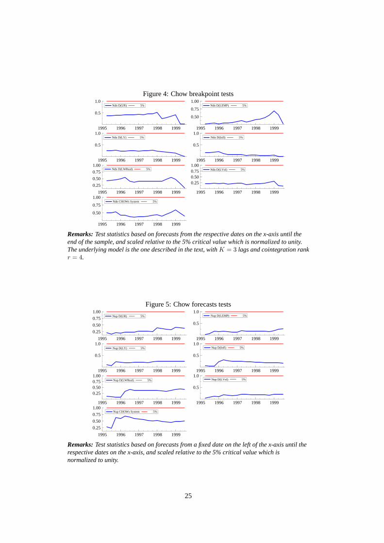
Figure 4: Chow breakpoint tests

1995 1996 1997 1998 1999

0.5

1.0Ndn D(UR) 5%

1995 1996 1997 1998 1999

0.50

0.75

1.00Ndn D(LEMP) 5%

1995 1996 1997 1998 1999

0.5

1.0Ndn D(LY) 5%

1995 1996 1997 1998 1999

0.5

1.0Ndn D(Infl) 5%

1995 1996 1997 1998 1999

0.25

0.50

0.75

1.00Ndn D(LWReal) 5%

1995 1996 1997 1998 1999

0.250.500.751.00

Ndn D(LVol) 5%

1995 1996 1997 1998 1999

0.50

0.75

1.00Ndn CHOWs System 5%

Remarks:Test statistics based on forecasts from the respective dates on the x-axis until theend of the sample, and scaled relative to the 5% critical value which is normalized to unity.The underlying model is the one described in the text, withK = 3 lags and cointegration rankr = 4.

Figure 5: Chow forecasts tests

1995 1996 1997 1998 1999

0.25

0.50

0.75

1.00Nup D(UR) 5%

1995 1996 1997 1998 1999

0.5

1.0Nup D(LEMP) 5%

1995 1996 1997 1998 1999

0.5

1.0Nup D(LY) 5%

1995 1996 1997 1998 1999

0.5

1.0Nup D(Infl) 5%

1995 1996 1997 1998 1999

0.250.500.751.00

Nup D(LWReal) 5%

1995 1996 1997 1998 1999

0.5

1.0Nup D(LVol) 5%

1995 1996 1997 1998 1999

0.25

0.50

0.75

1.00Nup CHOWs System 5%

Remarks:Test statistics based on forecasts from a fixed date on the left of the x-axis until therespective dates on the x-axis, and scaled relative to the 5% critical value which isnormalized to unity.

25

Figure 6:

1996 1997 1998 1999 2000

0.5

1.01up D(LEMP) 1%

1996 1997 1998 1999 2000

0.5

1.01up D(LY) 1%

1996 1997 1998 1999 2000

0.5

1.01up D(Infl) 1%

1996 1997 1998 1999 2000

0.5

1.01up D(LWReal) 1%

1996 1997 1998 1999 2000

0.5

1.01up D(LVol) 1%

1996 1997 1998 1999 2000

0.5

1.01up D(UR) 1%

1996 1997 1998 1999 2000

0.5

1.01up CHOWs system 1%

Remarks:The Chow test statistics are based on recursive 1-step forecast errors that are scaledrelative to the (1%) critical value which is normalized to unity.

26

Figure 7: VECM forecasts, break date 1999q4

19992000

2001

0.10

0.12F

orecasts U

R

19992000

2001

9.950

9.975

10.000F

orecasts LE

MP

19992000

2001

14.55

14.60

14.65F

orecasts LY

19992000

2001

−2.5

0.0

2.5

5.0F

orecasts Infl

19992000

2001−

4.25

−4.20

−4.15

Forecasts

LWR

eal

19992000

2001

13.52

13.53

13.54

13.55F

orecasts LV

ol

Remarks: The bands denote the 95% forecast confidence intervals taking into account theinnovation variance as well as parameter uncertainty.

27

Figure 8: VECM forecasts, break date 2000q1

19992000

2001

0.09

0.10

0.11

0.12F

orecasts U

R

19992000

2001

9.950

9.975

10.000F

orecasts LE

MP

19992000

200114.55

14.60

14.65F

orecasts LY

19992000

2001

−2.5

0.0

2.5

5.0F

orecasts Infl

19992000

2001

−4.20

−4.15

Forecasts

LWR

eal

19992000

2001

13.53

13.54

13.55

13.56F

orecasts LV

ol

Remarks: The bands denote the 95% forecast confidence intervals taking into account theinnovation variance as well as parameter uncertainty. The estimation sample includes the ob-servation 1999q4, but corrected with an impulse dummy due to the stability failure documentedin figure6.

28

Tables

Table 1: Comparison of the macroeconomic context between France and the EurozoneEU EU w/o Fr France EU EU w/o Fr France EU EU w/o Fr France EU EU w/o Fr France

real GDP1 Employment1 Labor costs1,2 Population1

1990 2.6 1.0 0.51991 1.0 0.2 2.8 0.51992 1.5 1.5 1.5 -0.9 -1.0 -0.7 7.3 7.7 5.9 0.5 0.5 0.51993 -0.8 -0.8 -0.9 -2.0 -2.2 -1.2 3.2 2.4 5.7 0.5 0.5 0.41994 2.4 2.4 2.1 -0.1 -0.1 0.2 2.5 2.5 2.2 0.3 0.3 0.41995 2.3 2.4 1.7 0.6 0.6 0.5 3.4 3.4 3.4 0.3 0.3 0.41996 1.4 1.5 1.1 0.6 0.6 0.5 2.8 2.9 2.3 0.3 0.3 0.31997 2.3 2.5 1.9 0.8 0.9 0.4 0.3 0.3 0.4 0.3 0.3 0.31998 2.9 2.7 3.4 1.9 1.9 1.7 0.8 0.5 1.8 0.2 0.2 0.41999 2.8 2.7 3.2 2.1 2.0 2.1 2.8 2.7 3.0 0.3 0.2 0.42000 3.5 3.4 3.8 2.3 2.3 2.5 2.7 2.8 2.2 0.4 0.3 0.52001 1.4 1.3 1.8 1.6 1.4 2.3 2.7 2.8 2.5 0.4 0.4 0.52002 0.8 0.7 1.2 0.4 0.3 0.6 2.5 2.5 2.6 0.4 0.3 0.5

Inflation rate (CPI)2 Employees1 Productivity1,5 Population (15-64)1

1990 1.5 1.61991 4.3 3.4 0.8 0.8 0.01992 3.8 2.5 -1.2 -1.4 -0.1 2.5 2.6 2.2 0.5 0.5 0.21993 3.4 2.2 -1.7 -1.9 -0.8 1.2 1.4 0.4 0.4 0.5 0.21994 2.8 1.7 -0.4 -0.6 0.6 2.4 2.6 1.9 0.3 0.3 0.21995 2.6 1.8 0.6 0.6 0.9 1.6 1.8 1.2 0.2 0.2 0.21996 2.3 2.3 2.1 0.5 0.5 0.8 0.8 0.9 0.6 0.2 0.2 0.31997 1.7 1.7 1.3 0.8 0.9 0.5 1.5 1.5 1.5 0.2 0.2 0.31998 1.2 1.3 0.7 2.0 2.0 1.9 1.0 0.8 1.7 0.2 0.1 0.31999 1.1 1.2 0.6 2.1 2.1 2.1 0.7 0.6 1.1 0.1 0.1 0.32000 2.1 2.2 1.8 2.4 2.3 2.8 1.1 1.1 1.2 0.2 0.2 0.42001 2.4 2.5 1.8 1.6 1.4 2.3 -0.2 -0.1 -0.4 0.3 0.2 0.42002 2.3 2.3 1.9 0.6 0.5 1.0 0.4 0.4 0.5 0.3 0.3 0.5

Real eff. exch. rate (CPI)2 Unemployment rate2,3 Unit labor costs1,2 Labor force1,4

1990 8.7 3.2 8.6 -1.61991 -2.8 -3.6 9.1 2.0 0.61992 3.7 1.3 10.0 4.8 5.1 3.6 0.0 -0.1 0.41993 -5.3 -2.2 10.1 9.9 11.3 2.0 1.0 5.4 0.0 -0.1 0.21994 -0.5 -0.6 10.8 10.6 11.8 0.1 -0.1 0.3 0.4 0.3 0.71995 6.2 1.4 10.6 10.4 11.3 1.8 1.6 2.2 0.4 0.4 0.31996 0.7 1.2 10.8 10.6 11.9 2.0 2.1 1.7 0.8 0.7 1.01997 -6.9 -2.9 10.8 10.6 11.8 -1.2 -1.2 -1.1 0.8 0.8 0.41998 2.7 0.4 10.2 10.0 11.4 -0.2 -0.3 0.1 1.3 1.4 1.01999 -3.8 -2.4 9.4 9.1 10.7 2.0 2.1 1.9 0.9 0.8 1.32000 -8.2 -5.8 8.5 8.3 9.3 1.5 1.7 1.0 1.1 1.1 1.02001 2.6 -0.5 8.0 7.9 8.5 2.9 2.9 3.0 0.9 0.8 1.02002 3.4 0.2 8.4 8.3 8.8 2.1 2.1 2.1 0.9 0.8 1.1All numbers are growth rates (yoy) in %, except for the unemployment rate, which is in level and in %. “EU” is the Euro area.1 AMECO, own calculations2 EUROSTAT, own calculations3 harmonized4 labor force statistics5 measured as output per headSource: AMECO, Eurostat, own calculations

29

Table 2: Different measures of working time1999q1 1999q2 1999q3 1999q4 2000q1 2000q2 2000q3 2000q4

ACEMO (2003)1 38.6 38.6 38.3 38.0 37.2 36.9 36.8 36.6-0.1 -0.2 -0.6 -0.7 -2.2 -0.7 -0.4 -0.4

DARES (2003)2 36.5 36.5 36.3 36.1 35.7 35.4 35.4 35.3-0.3 0.0 -0.5 -0.6 -1.1 -0.7 -0.2 -0.2

our data3 38.7 38.7 38.6 38.4 38.0 37.7 37.5 37.4-0.1 -0.1 -0.3 -0.5 -1.0 -1.0 -0.4 -0.3

The numbers in italics are quarterly growth rates in %.1 Working time published by the MES-DARES from the poll ACEMO. This data refers to firms with more than10 employees and full-time employees. It stems from the DARES database (as of November 2003).2 Working-time calculated by the MES-DARES correcting the results of ACEMO for firms with less than10 employees and part-time employees. It corrects additionally for a statistical break of the definition of theworking-time in 2000 induced by AUBRY II. This figure was published in the DARES database (as of Novem-ber 2003). Note that this series could not be used in our analysis because it only dates back to 1993.3 See the appendix for the exact calculation.

Table 3: Description of the data

Abbrev. Meaning Source / details

UR unemployment rate Standardized unemployment rate (ILOconcept) from the OECD.

LEMP number of employed workers(log of)

Source INSEE.

LY real GPD (1995 prices, log of) From OECD Main Economic Indica-tors (MEI).

LPY GDP deflator (log of) From OECD MEI. The first difference(times 400 to achieve approximate an-nual growth rates) is the inflation ratemeasure,Inflt ≡ 400 ∗∆LPYt.

LW hourly wage (log of) Total compensation taken from thequarterly national accounts of theOECD (QNA) and then divided by thelabor volume, see below.

LVol labor input volume of employedworkers (hours, log of)

See the appendix.

30

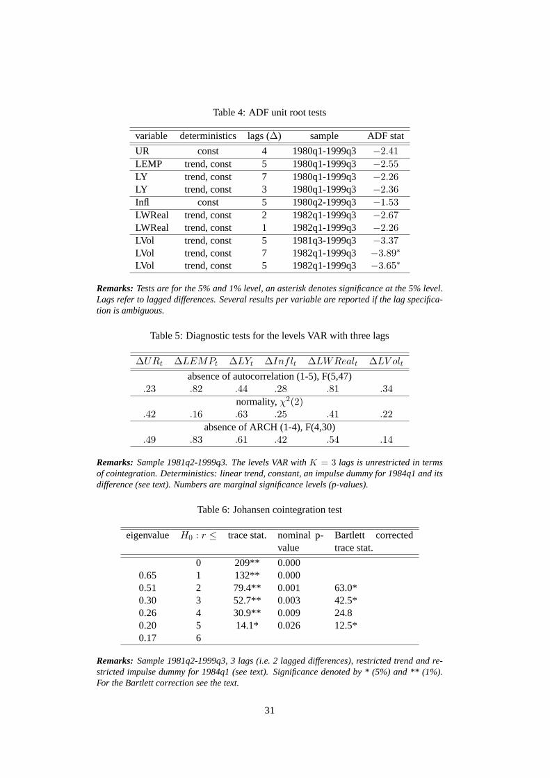
Table 4: ADF unit root tests

variable deterministics lags (∆) sample ADF stat

UR const 4 1980q1-1999q3 −2.41LEMP trend, const 5 1980q1-1999q3 −2.55LY trend, const 7 1980q1-1999q3 −2.26LY trend, const 3 1980q1-1999q3 −2.36Infl const 5 1980q2-1999q3 −1.53LWReal trend, const 2 1982q1-1999q3−2.67LWReal trend, const 1 1982q1-1999q3−2.26LVol trend, const 5 1981q3-1999q3 −3.37LVol trend, const 7 1982q1-1999q3 −3.89∗

LVol trend, const 5 1982q1-1999q3 −3.65∗

Remarks:Tests are for the 5% and 1% level, an asterisk denotes significance at the 5% level.Lags refer to lagged differences. Several results per variable are reported if the lag specifica-tion is ambiguous.

Table 5: Diagnostic tests for the levels VAR with three lags

∆URt ∆LEMPt ∆LYt ∆Inflt ∆LWRealt ∆LV olt

absence of autocorrelation (1-5), F(5,47).23 .82 .44 .28 .81 .34

normality,χ2(2).42 .16 .63 .25 .41 .22

absence of ARCH (1-4), F(4,30).49 .83 .61 .42 .54 .14

Remarks:Sample 1981q2-1999q3. The levels VAR withK = 3 lags is unrestricted in termsof cointegration. Deterministics: linear trend, constant, an impulse dummy for 1984q1 and itsdifference (see text). Numbers are marginal significance levels (p-values).

Table 6: Johansen cointegration test

eigenvalue H0 : r ≤ trace stat. nominal p-value

Bartlett correctedtrace stat.

0 209** 0.0000.65 1 132** 0.0000.51 2 79.4** 0.001 63.0*0.30 3 52.7** 0.003 42.5*0.26 4 30.9** 0.009 24.80.20 5 14.1* 0.026 12.5*0.17 6

Remarks:Sample 1981q2-1999q3, 3 lags (i.e. 2 lagged differences), restricted trend and re-stricted impulse dummy for 1984q1 (see text). Significance denoted by * (5%) and ** (1%).For the Bartlett correction see the text.

31