Testing the level of consistency between choices and ... · Testing the level of consistency between choices and beliefs in ... Costa-Gomes and ... A low level of consistency between

Testing the level of consistency between choices and beliefs in

games using eye-tracking

Luca Polonioa,b*

and Giorgio Coricellic

a Department of Economics, University of Minnesota, 4-101 Hanson Hall, Minneapolis, MN 55455,

USA. E-mail: [email protected], Tel.+393881990266

b Center for Mind/Brain Sciences, CIMec, University of Trento, Palazzo Fedrigotti – corso Bettini

31, 38068 Rovereto, Trento, Italy.

c Department of Economics, University of Southern California, 3620 S Vermont Ave 300, Los

Angeles, CA 90089, USA. E-mail: [email protected]

*To whom correspondence should be sent

Abstract

We use eye-tracking technique to test whether players’ actions are consistent with their expectations

of their opponent’s behavior. Participants play a series of two-player 3 by 3 one shot games and

state their beliefs about which actions they expect their counterpart to play (first-order beliefs) or

about which actions their counterparts expect them to play (second-order beliefs). We perform a

mixed model cluster analysis and classify participants into types according to both their attentional

patterns of visual information acquisition and choices. Players classified as strategic (Level-2

players) and players classified as having other-regarding preferences like Inequity aversion and

Prosociality exhibit patterns of visual attention and choices that are mainly consistent with their

stated beliefs. Conversely, players classified as non-strategic (Level-1, Pessimistic, Optimistic and

Competitive) do not best respond to any specific belief, but apply simple decision rules regardless of

whether they are playing or stating their beliefs. Thus, using eye-tracking data we could identify a

larger consistency between actions and stated beliefs compared with previous studies, and we could

characterize the behavioral rules associated with choice-beliefs inconsistency. Implications for the

theories of bounded rationality are discussed.

Keywords: Game theory, beliefs, bounded rationality, eye-tracking

JEL classification: C72, C51, D84

mailto:[email protected]

2

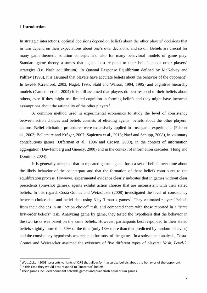
1 Introduction

In strategic interactions, optimal decisions depend on beliefs about the other players’ decisions that

in turn depend on their expectations about one’s own decisions, and so on. Beliefs are crucial for

many game-theoretic solution concepts and also for many behavioral models of game play.

Standard game theory assumes that agents best respond to their beliefs about other players’

strategies (i.e. Nash equilibrium). In Quantal Response Equilibrium defined by McKelvey and

Palfrey (1995), it is assumed that players have accurate beliefs about the behavior of the opponent1.

In level-k (Crawford, 2003; Nagel, 1995; Stahl and Wilson, 1994, 1995) and cognitive hierarchy

models (Camerer et al., 2004) it is still assumed that players do best respond to their beliefs about

others, even if they might use limited cognition in forming beliefs and they might have incorrect

assumptions about the rationality of the other players2.

A common method used in experimental economics to study the level of consistency

between action choices and beliefs consists of eliciting agents’ beliefs about the other players’

actions. Belief elicitation procedures were extensively applied in trust game experiments (Fehr et

al., 2003; Bellemare and Krôger, 2007; Sapienza et al., 2013; Naef and Schupp, 2008), in voluntary

contributions games (Offerman et al., 1996 and Croson, 2000), in the context of information

aggregation (Duwfemberg and Gneezy, 2000) and in the context of information cascades (Hung and

Dominitz 2004).

It is generally accepted that in repeated games agents form a set of beliefs over time about

the likely behavior of the counterpart and that the formation of these beliefs contributes to the

equilibration process. However, experimental evidence clearly indicates that in games without clear

precedents (one-shot games), agents exhibit action choices that are inconsistent with their stated

beliefs. In this regard, Costa-Gomes and Weizsäcker (2008) investigated the level of consistency

between choice data and belief data using 3 by 3 matrix games3. They estimated players’ beliefs

from their choices in an “action choice” task, and compared them with those reported in a “state

first-order beliefs” task. Analyzing game by game, they tested the hypothesis that the behavior in

the two tasks was based on the same beliefs. However, participants best responded to their stated

beliefs slightly more than 50% of the time (only 18% more than that predicted by random behavior)

and the consistency hypothesis was rejected for most of the games. In a subsequent analysis, Costa-

Gomes and Weizsäcker assumed the existence of five different types of players: Nash, Level-2,

1 Weizsäcker (2003) presents variants of QRE that allow for inaccurate beliefs about the behavior of the opponent.

2 In this case they would best respond to “incorrect” beliefs.

3 Their games included dominant solvable games and pure Nash equilibrium games.

3

Level-1, Dominance-1 and Optimistic. Among these five models, the Level-1 model4 described the

action data best. However, when the players stated their first-order beliefs, they attributed their own

level of sophistication to the other players. This behavior is inconsistent because if players believe

their counterpart to be Level-1 they should best respond to this belief, acting like a Level-2 player5.

The authors explained this inconsistency by stating that there is a general and significant difference

in the perception of the games and/or of how players’ counterparts play games6.

A low level of consistency between choices and stated beliefs was found also by Nyarko and

Schotter (2002). In a series of two person constant sum game experiments, the authors tested the

explanatory power of different belief-learning models and found that they do not predict stated

beliefs well. Conversely, Ivanov (2006 mimeo) and Rey Biel (2009) conducted experiments similar

to that of Costa-Gomes and Weizsäcker and found a higher level of consistency between action

choices and stated beliefs. They also used 3x3 normal form games but their games were simpler

than those of Costa-Gomes and Weizsäcker. The difference in the results obtained by different

investigators emphasizes the importance of the complexity of the environment and suggests that

inconsistency between choices and beliefs increases with increasing complexity of the decision

problem.

Another aspect to be taken into account when assessing the level of consistency between

choices and beliefs is related to the existence of heterogeneity in interdependent preferences. A

number of studies have reported a significant proportion of participants whose behavior is

consistent with different motives such as Inequity Aversion, Prosociality and Competition

(Andreoni and Miller, 2002; Fisman et al., 2007; Blanco et al., 2011; Iriberri and Rey-Biel, 2013;

Polonio et al., 2015). Heterogeneity in interdependent preferences requires defining the best

response for each agent’s belief based on her type. Therefore, to assess the level of consistency

between choices and beliefs we need to define, with precision, the interdependent preferences of

each agent, assuming that these preferences remain constant over the games the agent plays.

The aim of our study is to explain the general inconsistency observed in the literature

between action choices and stated belief data. To reach this goal, we used both choice and eye-

tracking data (i.e. lookup patterns) to associate participants with different decision rules; then their

stated beliefs about the actions of their counterpart and their stated beliefs about the stated beliefs of

their counterpart (second-order beliefs) were predicted based on their type. The analysis of the eye

movements allowed us to clearly distinguish between participants using different decision rules, and

4 Level-1 players best respond to a uniform probability belief over the actions of their counterpart.

5 Their results were shown to be independent to the order of the two tasks (“action choices” and “state beliefs”).

6 They also performed additional tests to exclude the possibility that inconsistency among choice data and belief data

are due to risk-aversion or other-regarding preferences. Their results ruled out these hypotheses.

4

more importantly, to identify those types of players who make choices without forming beliefs

about the expected action of their counterpart.

We started from the assumption that players' behavior is determined by decision rules or

types that can be defined by the interaction between two general components: the motives that drive

players’ actions and the level of sophistication that can be reached by the players. Following this

theoretical framework, we extended the Costa-Gomes and Weizsäcker study in six ways. Firstly, we

consider the possibility that players are guided by different motivations when choosing their

actions7. In this respect, we take into account a larger set of models that can be summarized as

follows: (1) “strategic sophistication-based models” including individualistic models having

different levels of sophistication (Equilibrium, Dominance-2, Dominance-1, Level-2 and Level-1

models). (2) “Risk-based models”, including individualistic models based on a high or low risk

propensity (Pessimistic and Optimistic models). (3) “Social preference-based models” including

Cooperative or Competitive models (Inequity Aversion, Prosocial and Competitive models).

Secondly, we used both attentional patterns of visual information search and choices to classify

players into different types; then, the level of consistency between action choices and beliefs was

estimated separately for each type. Thirdly, the information search analysis allowed us to evaluate

differences and similarities between the visual information acquisition patterns used by the agents

when choosing actions and stating their beliefs. Fourthly, we added (four) games with multiple

equilibria to the set of games used by Costa-Gomes and Weizsäcker, in order to evaluate possible

differences in the decision process in a wider range of games. Fifthly, we added a treatment in

which players have to guess what other players think they will choose (“state second-order beliefs

task”). This treatment was introduced in order to better evaluate the hypothesis of level-k and

cognitive hierarchy models regarding the belief based hierarchy of players8. Sixth, at the end of the

two tasks (action choices and belief statements tasks), participants were asked to complete

questionnaires analyzing their cognitive abilities (Unsworth and Engle, 2007; Walsh and Betz,

1995; Frederick, 2005), their risk attitude (Holt and Laury, 2002) and their social value orientation

(Van Lange and Liebrand, 1991; Murphy et al., 2011), in order to assess possible correlations

among variables related to strategic behavior (choices, belief statements and eye-movements) and

different aspects related to cognition and personality traits.

7 It is important to notice that Costa-Gomes and Weizsäcker included only individualistic types in their analyses. The

authors test whether the behavior of the players was driven by pure altruism (the willingness to choose the action that gives the counterpart the highest average payoff) or by Rawlsian preferences (the willingness to choose the action that maximize the lowest of the two players’ payoffs), but they did not test for the presence of agents with Inequity averse, Prosocial or Competitive attitudes. 8 For example, players classified as Level-2 are supposed to give the best response to the belief that their counterpart

is a level-1 player (level k models) or a mix of level-1 and level-0 players. Following the CH model, these players’ should believe that their counterpart believes that they are not more sophisticated than level-0.

5

We hypothesize that the level of consistency between choices and beliefs depends on the decision

rule adopted by the participant. More precisely, we hypothesize that sophisticated players

(Equilibrium, Dominance-2, Dominance-1 and Level-2) exhibit action choices that are mainly

consistent with their stated beliefs regarding the choice of their counterparts. Conversely, we

propose that less sophisticated players (Level-1, Pessimistic, Optimistic and Competitive) do not

form beliefs about the other player’s strategy but apply simple decision rules as if they were not

involved in any strategic interaction. Finally we hypothesize that players with other-regarding

preferences such as Inequity aversion and Prosociality want to coordinate their actions with those of

the counterpart and believe that the other player is doing likewise.

With our eye-tracking study, we identified the underlying reasoning processes adopted by

different agents in action choices and stated beliefs tasks and we were able to distinguish between

players who hold a clear set of beliefs about the other players' strategies and players who apply

simple decision rules regardless of whether they are playing or stating their beliefs.

2 Experimental design

2.1 Games and models of game play

We selected eighteen games including the fourteen games used in Costa-Gomes and Weizsäcker

study plus four games with multiple equilibria. These games allowed us to distinguish among ten

models of game play. The models were selected in order to have a large variability in terms of level

of sophistication (Nash Equilibrium, Dominance-2, Dominance-1, Level-2, Level-1), risk propensity

(Pessimistic and Optimistic) and other-regarding preferences (Inequity aversion, Prosociality and

Competition)9, three dimensions which have proved to be important as determinants of behavior in

interactive game playing. The ten models are summarized as follow:

1) Nash equilibrium model (EQ): players choosing according to the equilibrium.

2) Dominance-2 model (“D2”, Costa-Gomes et al., 2001): players selecting a best response

to a uniform prior over their partner's remaining decisions after applying two rounds of

deleting dominated strategies.

3) Dominance-1 model (“D1”, Costa-Gomes et al., 2001): players selecting a best response

against a uniform probability distribution of belief over the opponent undominated

actions only and zero otherwise.

9 The models included the five models adopted in Costa-Gomes and Weizsäcker study (Nash, Level-2, Dominance-1,

Level-1 and Optimistic) plus another five models that allowed for the possibility that the agents have other-regarding preferences (Inequity Averse, Prosocial, Competitive), are risk averse (Pessimistic) or perform two rounds of deleting dominated strategies (Dominance-2).

6

4) Level-2 model (“L2”, Stahl and Wilson, 1994, 1995, Nagel, 1995, and Costa-Gomes et

al., 2001): players selecting a best response to level-1 players.

5) Level-1 or Naïve model (“L1”, Stahl and Wilson, 1994, 1995, Costa-Gomes et al., 2001):

players selecting a best response against the uniform probability distribution of belief

over the opponent’s actions.

6) Pessimistic model (“Pess”, Haruvy et al., 1999): players selecting the option with the

highest minimum payoff.

7) Optimistic model (“Opt”, Haruvy et al., 1999): players selecting the option with the

highest payoff.

8) Inequity Aversion model (“IA”, Fehr and Schmidt, 1999): players selecting the option

that minimizes the difference between their own payoff and the payoff of their

counterpart.

9) Prosocial or cooperative model (“Pros”, Van Lange, 2000, defined as altruistic in Costa-

Gomes et al., 2001): players selecting the option that maximizes the joint payoff.

10) Competitive (“Comp”, Van Lange, 2000): players selecting the option that maximizes

the difference between their own payoff and the payoff of their counterpart.

Game Dominance

solvable

Rounds

of dom.

EQ

(Pareto)

D2 D1 L2 L1 Pess Opt IA Pros Comp

1 Y 2,3 T-L T-L T-L T-M M-L M-L B-M T-L B-R M-M

2 Y 3,2 M-L M-L M-L T-L M-M M-M T-R M-L B-R M-M

3 Y 2,3 B-R B-R B-M B-M T-M T-R M-M T-M T-M T-M

4 Y 3,2 M-M M-M T-M T-M T-L M-L T-R T-L T-L T-L

5 Y 2,3 T-M T-M T-L T-L B-L B-L M-L B-L B-R B-L

6 Y 3,2 B-M B-M M-M M-M M-R M-R M-L M-M T-R M-R

7 Y 2,3 M-R T-R M-R M-R B-R B-M T-M T-L T-L M-R

8 Y 3,2 B-R M-R B-R B-R B-L B-L T-M M-M M-M T-R

9 Y 3,4 T-R T-M T-M M-R T-L T-M M-L T-R T-R T-M

10 Y 4,3 B-L M-L M-L B-M T-L M-L T-M B-L B-L M-L

11 N –,– M-M B-M B-M M-R B-M B-M T-L M-M T-R B-M

12 N –,– B-L M-R M-R M-M M-R M-R T-L B-L B-L M-R

13 N –,– T-R T-M T-M B-R T-M T-M M-L T-R B-L T-M

14 N –,– T-L B-M B-M M-M B-M B-M T-R T-L T-L B-M

15 N –,– (T-L) B-R B-R B-R B-R B-R T-L T-L T-L B-R

16 N –,– (M-M) T-L T-L T-L T-L T-L M-M M-M M-M T-L

17 N –,– (B-L) M-R M-R M-R M-R M-R B-L B-L B-L M-R

18 N –,– (B-M) T-R T-R T-R T-R T-R B-M B-M B-M T-R

Table 1: Strategic structures of the 18 games and actions predicted by the 10 models. In the third column of the Table

are shown the number of rounds of dominance required by row and column players to reach the equilibrium. For the

Nash equilibrium model, in games with multiple equilibria (games from 15 to 18), we reported (in brackets) the actions

in accordance with the Pareto equilibria.

7

Game 1 L M R Game 2 L M R

T 78,73 69,23 12,14 T 21,67 59,57 85,63

M 67,52 59,61 78,53 M 71,76 50,65 74,14

B 16,76 65,87 94,79 B 12,10 51,76 77,92

Game 2’s payoffs are obtained by subtracting 2 points from Game 1’s payoffs.


T 74,38 78,71 46,43 T 73,80 20,85 91,12

M 96,12 10,89 57,25 M 45,48 64,71 27,59

B 15,51 83,18 69,62 B 40,76 53,17 14,98

Game 4’s payoffs are obtained by adding 2 points to Game 3’s payoffs.


T 78,49 60,68 27,35 T 39,99 36,28 57,86

M 10,82 49,10 98,38 M 83,11 50,79 65,70

B 69,64 42,39 85,56 B 11,50 69,61 40,43

Game 6’s payoffs are obtained by adding 1 points to Game 5’s payoffs.


T 84, 82 33, 95 12, 73 T 47, 30 94, 32 36, 38

M 21, 28 39, 37 68, 64 M 38, 69 81, 83 27, 20

B 70, 39 31, 48 59, 81 B 80, 58 72, 11 63, 67

Game 8’s payoffs are obtained by subtracting 1 points from Game 7’s payoffs.


T 57, 58 46, 34 74, 70 T 60, 59 34, 91 96, 43

M 89, 32 31, 83 12, 41 M 36, 48 85, 33 39, 18

B 41, 94 16, 37 53, 23 B 72, 76 43, 14 25, 55

Game 10’s payoffs are obtained by adding 2 points from Game 9’s payoffs.


T 43, 91 38, 81 92, 64 T 25,27 90, 43 38, 60

M 39, 27 79, 68 68, 19 M 49, 39 53, 73 78, 52

B 69, 10 66, 21 74, 54 B 64, 85 20, 46 19,78


T 83, 40 23, 68 70, 81 T 82, 61 36, 46 24, 22

M 93, 45 12, 71 29, 41 M 43, 17 70, 50 40, 87

B 66, 94 56, 76 21, 70 B 75, 16 49, 75 57, 35

Game 13’s payoffs are obtained by adding 2 points from Game 11’s payoffs. Game 14’s payoffs are obtained by

subtracting 3 points from Game 12’s payoffs.


T 73, 73 34,22 17, 55 T 68, 68 62, 22 60, 59

M 22, 34 68, 68 54, 57 M 39, 62 78, 78 22, 27

B 55, 17 57, 55 63, 63 B 59, 60 27, 39 73, 73


T 25, 37 71,71 57,60 T 62, 61 64, 24 70, 70

M 58, 20 60, 57 66,66 M 75, 75 61, 41 29, 62

B 76,76 37,25 20,58 B 24, 29 80, 80 41, 64

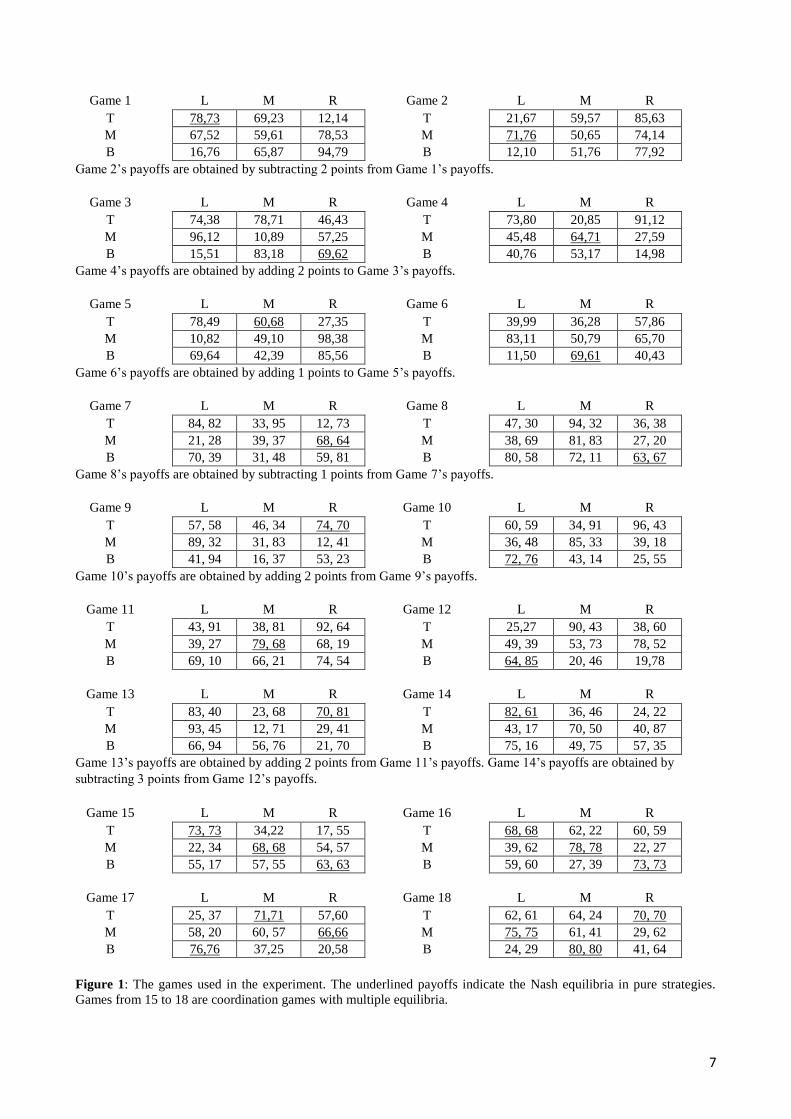
Figure 1: The games used in the experiment. The underlined payoffs indicate the Nash equilibria in pure strategies.

Games from 15 to 18 are coordination games with multiple equilibria.

8

In Table 1, a description of the strategic structure of the eighteen games is given and the action

predictions of the ten models of game play presented. Ten of our games are solvable in two, three or

four steps of iterated dominance, four games have unique Nash equilibrium without dominant

strategies and four games are weak-link games (a 3 by 3 version of the stag-hunt games) with three

equilibria, one of which is Pareto optimal. Games with unique pure-strategy equilibrium do not

contain salient payoffs. Conversely, weak-link games include possible game solutions that may act

as attractors. As shown in Figure 1, the games with unique pure-strategy equilibrium (games from 1

to 14) are organized into seven pairs of isomorphic games. The second game of each pair is

identical to the first except for transposing the players’ roles, changing the order of the three actions

for the two players and adding or subtracting a constant small amount to the payoffs of each game.

Using pairs of isomorphic games all participants face the same sets of games regardless of the role

they play (row or column). Importantly, participants cannot be aware of this because of the uniform

payoffs shift. In coordination games, we do not need to have pairs of isomorphic games because

each game has an isomorphic structure.

2.2 Overall structure

Our experimental design consisted of four treatments of two sessions each. The treatments were

defined as follows: in treatment “A1T”, players chose their action “A” (in all the 18 games) before

stating their first-order beliefs “1”. In treatment “A2T”, players chose their action “A” (in all the 18

games) before stating their second-order beliefs “2”. In treatment “1AT”, players stated their first-

order beliefs “1” (in all the 18 games) before choosing their action “A”. “T” indicates that eye

movements were recorded in the three treatments. Finally, in treatment “A1” players chose their

actions “A” (in all the 18 games) before stating their first-order beliefs “1” and eye-movements

were not recorded. Treatment “A1” have been included in order to control for possible effects due to

the eye-tracking apparatus. Participants were equally and randomly divided in row and column

players within each treatment.

All sessions were run at the EPL lab (Experimental Psychology Laboratory) of the

University of Trento. Participants were 128 undergraduate students at the University of Trento (42

males, 86 females), the mean age was 23 (SD 3.16). Presentation of the stimuli was performed

using a custom made program implemented using the Matlab Psychophysical toolbox.

Before the experiments started, a copy of preliminary instructions, which described a 3 by 3

strategic situation, was given to the participants and read aloud by the experimenter. The

participants were required to pass a comprehension test in which they had to demonstrate that they

knew how to map players’ actions in a game to outcomes and outcomes to players’ payoffs.

9

Participants who failed the test were dismissed. Excluding these participants, we had 28, 28, 28 and

44 participants in treatments A1T, A2T, 1AT, A1 respectively.

Participants in treatments A1T first read the instructions about how to choose their actions

and how they would be rewarded in the action choice task. After the eye-tracking system was

calibrated, participants underwent two practice games, and then played the 18 games (session I). At

the end of the first session, participants read the instructions on how to state their beliefs and how

they would be rewarded for the accuracy of their statements. Next, they stated their first-order

beliefs in all the 18 games10

(session II) without knowing in advance the outcome of their actions.

No time limit was imposed on participants to give their response. At the end of the two

sessions, participants were asked to complete questionnaires assessing their cognitive abilities,

social value orientation and risk propensity (session III). We administered an immediate free recall

working memory test (Unsworth and Engle, 2007), the Wechsler digit span test for short-term

memory (Walsh and Betz, 1995), the Cognitive Reflection Test (Frederick, 2005), a social value

orientation test (Murphy et al., 2011) and a risk aversion test without real payments (Holt and

Laury, 2002). Participants were paid for their decisions in the social value orientation test.

In treatment A2T, the order of the tasks was the same but the instructions and the tasks in

session II were about stating second-order beliefs. In treatment A1, the order was the same, except

that we did not record eye-tracking data. In treatment 1AT, the order was reversed, and the

participants stated all 18 first-order beliefs before they played the games. Participants first read the

instructions about how to choose their actions and how they would be rewarded in the action choice

task. Then, they read the instructions on first-order stated beliefs and how they would be rewarded

for the accuracy of their statements. Next, they stated their beliefs for all 18 games and finally they

played the 18 games.

Because of the peculiar characteristics of eye-tracking experiments, all participants were

tested individually. At the beginning of the experiment, the experimenter told the participants that

their responses would be paired with those of a randomly selected opponent belonging to the same

experimental treatment11

, and it was made clear that in each game they were facing the same

opponent when playing the game and when stating their beliefs. No feedback about the result of

their decisions was given to the participants until the end of the data collection. At the end of the

data collection, participants were anonymously and randomly paired, and their responses were

combined.

All participants returned to receive their payments a few days after the end of the experiment

and everyone drew three tags from three different jars. Each of the tags in the first and second jars 10

Two practice trials were administered before beginning the state first-order belief task. 11

Except for players in treatment A2T which were paired with players in treatment A1T and vice-versa.

10

was associated with one of the games used during the experiment. The tag extracted from the first

jar determined the payment for the action choice task and the tag extracted from the second jar

determined the payment for the belief elicitation task. Each of the tags in the third jar was

associated with a Social Value Orientation (SVO) slider item and the slider item extracted was used

to determine the payments for the SVO questionnaire.

For the action choice task, participants were paid at a rate of 10 cents per point. For the first

and second-order belief tasks participants were paid 5 Euro when their prediction was correct and 0

otherwise. For the SVO questionnaire, participants were paid 5 cents per point. They earned

between 1.75 and 19.9 Euro in addition to 4 Euro show-up fee. 10 participants in the eye-tracking

treatments were discarded due to poor calibration (see the eye-tracking procedure described in

section 5.1) and 1 participant in treatment A1 was discarded due to technical reasons. We collected

eye-tracking and behavioral data for 28, 19, 27 participants in treatments A1T, A2T, 1AT,

respectively and behavioral data for 43 participants in treatment A1. The ethical committee of the

University of Trento approved the study, and all participants gave informed consent prior to

admission into the study.

3 Results: Choices and beliefs

3.1 Testing for treatment effects

As in Costa-Gomes and Weizsäcker we evaluated possible treatment effects. We expected to

replicate their findings, showing small differences due to the order of tasks and the players’ role.

Furthermore, we expected no significant differences due to the use of the eye-tracking apparatus in

action choices and stated beliefs.

We used Fisher’s exact probability test to check whether the belief statement task has an

effect on actions12

. We paired the treatments (A1T, A2T, 1AT, A1) in all possible ways and

compared the participants’ aggregate actions separately for each of the 18 games. We found 4 p-

values lower than 5% (significance level), well within the limits of chance (10.8) for 216

comparisons (in A1T play vs. 1AT play in game 7, A1T play vs. A2T play in game 10, A1T play vs.

1AT play in game 11, and in 1AT play vs. A2T play in game 17). To control for possible learning

effects in the absence of feedback, we tested the hypothesis that the actions of Row and Column

players (within each treatment) in isomorphic or in pairs of isomorphic games were drawn from the

same distribution. This hypothesis was rejected for only two comparisons (in A1T row play in game

2 vs. Column play in game 1, and in A2T row play in game 13 vs. Column play in game 11), which

is within the limits of chance (3.6) for 72 comparisons. Based on these results we pooled the data of

12

This analysis was conducted without aggregating row and column players.

11

row and column players within each treatment and compared the players’ actions across treatments

again. We found only 3 comparisons with a p-value lower than 5%, which is within the limit of

chance (5.4) for 108 comparisons (in A1T play vs. 1AT play in game 2, in 1AT play vs. AT2 play in

game 10, AT2 play vs. A1 play in game 10). Overall, our results show that participants’ aggregate

actions are not affected by the order of the tasks or the usage of the eye-tracking device. The same

analyses were repeated using the stated beliefs data. Once again, we found that the treatments have

a non-significant effect on the aggregate belief statements.

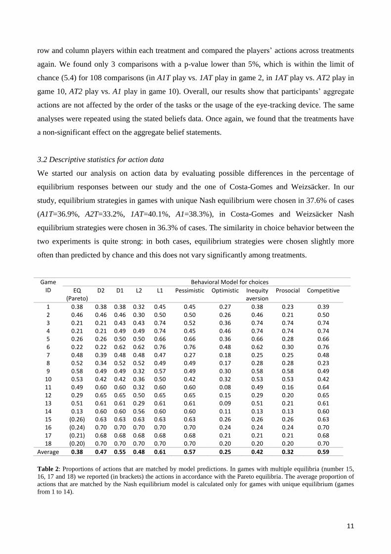
3.2 Descriptive statistics for action data

We started our analysis on action data by evaluating possible differences in the percentage of

equilibrium responses between our study and the one of Costa-Gomes and Weizsäcker. In our

study, equilibrium strategies in games with unique Nash equilibrium were chosen in 37.6% of cases

(A1T=36.9%, A2T=33.2%, 1AT=40.1%, A1=38.3%), in Costa-Gomes and Weizsäcker Nash

equilibrium strategies were chosen in 36.3% of cases. The similarity in choice behavior between the

two experiments is quite strong: in both cases, equilibrium strategies were chosen slightly more

often than predicted by chance and this does not vary significantly among treatments.

Game ID

Behavioral Model for choices

EQ (Pareto)

D2 D1 L2 L1 Pessimistic Optimistic Inequity aversion

Prosocial Competitive

1 0.38 0.38 0.38 0.32 0.45 0.45 0.27 0.38 0.23 0.39 2 0.46 0.46 0.46 0.30 0.50 0.50 0.26 0.46 0.21 0.50 3 0.21 0.21 0.43 0.43 0.74 0.52 0.36 0.74 0.74 0.74 4 0.21 0.21 0.49 0.49 0.74 0.45 0.46 0.74 0.74 0.74 5 0.26 0.26 0.50 0.50 0.66 0.66 0.36 0.66 0.28 0.66 6 0.22 0.22 0.62 0.62 0.76 0.76 0.48 0.62 0.30 0.76 7 0.48 0.39 0.48 0.48 0.47 0.27 0.18 0.25 0.25 0.48 8 0.52 0.34 0.52 0.52 0.49 0.49 0.17 0.28 0.28 0.23 9 0.58 0.49 0.49 0.32 0.57 0.49 0.30 0.58 0.58 0.49

10 0.53 0.42 0.42 0.36 0.50 0.42 0.32 0.53 0.53 0.42 11 0.49 0.60 0.60 0.32 0.60 0.60 0.08 0.49 0.16 0.64 12 0.29 0.65 0.65 0.50 0.65 0.65 0.15 0.29 0.20 0.65 13 0.51 0.61 0.61 0.29 0.61 0.61 0.09 0.51 0.21 0.61 14 0.13 0.60 0.60 0.56 0.60 0.60 0.11 0.13 0.13 0.60 15 (0.26) 0.63 0.63 0.63 0.63 0.63 0.26 0.26 0.26 0.63 16 (0.24) 0.70 0.70 0.70 0.70 0.70 0.24 0.24 0.24 0.70 17 (0.21) 0.68 0.68 0.68 0.68 0.68 0.21 0.21 0.21 0.68 18 (0.20) 0.70 0.70 0.70 0.70 0.70 0.20 0.20 0.20 0.70

Average 0.38 0.47 0.55 0.48 0.61 0.57 0.25 0.42 0.32 0.59

Table 2: Proportions of actions that are matched by model predictions. In games with multiple equilibria (number 15,

16, 17 and 18) we reported (in brackets) the actions in accordance with the Pareto equilibria. The average proportion of

actions that are matched by the Nash equilibrium model is calculated only for games with unique equilibrium (games

from 1 to 14).

12

Table 2 shows the proportions of actions that are matched by each of the ten models listed in Table

113

. Similarly to the results obtained by Costa-Gomes and Weizsäcker, Table 1 shows that the level-

1 model on average describes the action data best. Participants chose the action predicted by this

model 61% of the time. Competitive and Pessimistic models describe the action data almost as well

as the level-1 model (59% and 57% respectively), but in games where the two models make

different predictions, level-1 almost always describes the data better than the Competitive and

Pessimistic models (see Table 2).

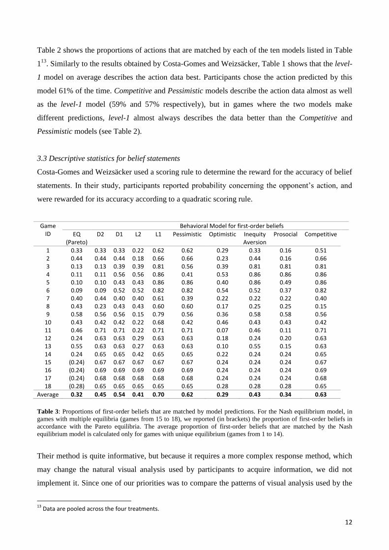
3.3 Descriptive statistics for belief statements

Costa-Gomes and Weizsäcker used a scoring rule to determine the reward for the accuracy of belief

statements. In their study, participants reported probability concerning the opponent’s action, and

were rewarded for its accuracy according to a quadratic scoring rule.

Game ID

Behavioral Model for first-order beliefs

EQ (Pareto)

D2 D1 L2 L1 Pessimistic Optimistic Inequity Aversion


1 0.33 0.33 0.33 0.22 0.62 0.62 0.29 0.33 0.16 0.51 2 0.44 0.44 0.44 0.18 0.66 0.66 0.23 0.44 0.16 0.66 3 0.13 0.13 0.39 0.39 0.81 0.56 0.39 0.81 0.81 0.81 4 0.11 0.11 0.56 0.56 0.86 0.41 0.53 0.86 0.86 0.86 5 0.10 0.10 0.43 0.43 0.86 0.86 0.40 0.86 0.49 0.86 6 0.09 0.09 0.52 0.52 0.82 0.82 0.54 0.52 0.37 0.82 7 0.40 0.44 0.40 0.40 0.61 0.39 0.22 0.22 0.22 0.40 8 0.43 0.23 0.43 0.43 0.60 0.60 0.17 0.25 0.25 0.15 9 0.58 0.56 0.56 0.15 0.79 0.56 0.36 0.58 0.58 0.56

10 0.43 0.42 0.42 0.22 0.68 0.42 0.46 0.43 0.43 0.42 11 0.46 0.71 0.71 0.22 0.71 0.71 0.07 0.46 0.11 0.71 12 0.24 0.63 0.63 0.29 0.63 0.63 0.18 0.24 0.20 0.63 13 0.55 0.63 0.63 0.27 0.63 0.63 0.10 0.55 0.15 0.63 14 0.24 0.65 0.65 0.42 0.65 0.65 0.22 0.24 0.24 0.65 15 (0.24) 0.67 0.67 0.67 0.67 0.67 0.24 0.24 0.24 0.67 16 (0.24) 0.69 0.69 0.69 0.69 0.69 0.24 0.24 0.24 0.69 17 (0.24) 0.68 0.68 0.68 0.68 0.68 0.24 0.24 0.24 0.68 18 (0.28) 0.65 0.65 0.65 0.65 0.65 0.28 0.28 0.28 0.65

Average 0.32 0.45 0.54 0.41 0.70 0.62 0.29 0.43 0.34 0.63

Table 3: Proportions of first-order beliefs that are matched by model predictions. For the Nash equilibrium model, in

games with multiple equilibria (games from 15 to 18), we reported (in brackets) the proportion of first-order beliefs in

accordance with the Pareto equilibria. The average proportion of first-order beliefs that are matched by the Nash

equilibrium model is calculated only for games with unique equilibrium (games from 1 to 14).

Their method is quite informative, but because it requires a more complex response method, which

may change the natural visual analysis used by participants to acquire information, we did not

implement it. Since one of our priorities was to compare the patterns of visual analysis used by the

13

Data are pooled across the four treatments.

13

players when they choose their actions and when they stated their beliefs, we kept the two tasks as

comparable as possible in terms of visual stimuli and type of response by asking the participants to

indicate which actions they expected their counterpart to choose (treatments A1T and 1AT) or which

action their counterpart expected them to choose (treatment A2T).

Equilibrium responses in games with unique-Nash equilibrium (from 1 to 14) were chosen

32.4% of the time in the first-order beliefs tasks (A1T=32.2%, 1AT=32.8%, A1=32.4%), and 29.7%

in the second-order beliefs tasks (A2T). Table 3 contains the proportion of stated first-order beliefs

that are matched by each of the ten models listed in Table 1, and shows that on average over the 18

games, belief statements follow the same pattern as action choices.

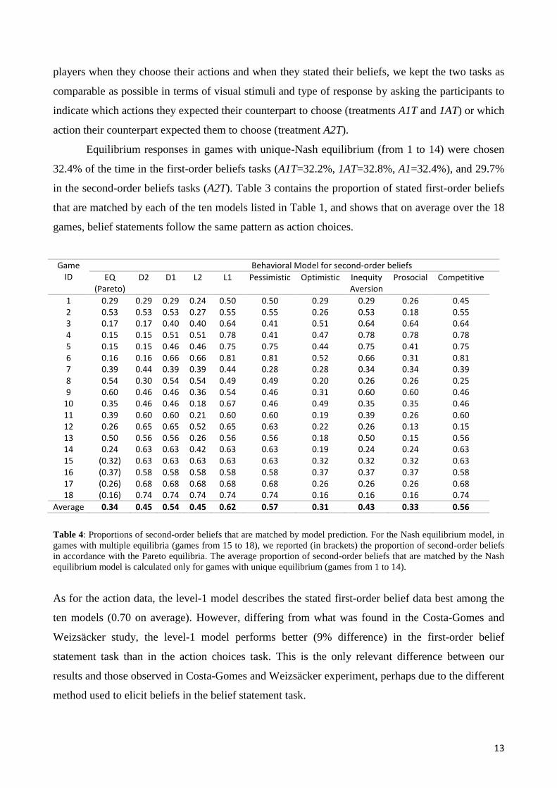
Game ID

Behavioral Model for second-order beliefs

EQ (Pareto)

D2 D1 L2 L1 Pessimistic Optimistic Inequity Aversion


1 0.29 0.29 0.29 0.24 0.50 0.50 0.29 0.29 0.26 0.45 2 0.53 0.53 0.53 0.27 0.55 0.55 0.26 0.53 0.18 0.55 3 0.17 0.17 0.40 0.40 0.64 0.41 0.51 0.64 0.64 0.64 4 0.15 0.15 0.51 0.51 0.78 0.41 0.47 0.78 0.78 0.78 5 0.15 0.15 0.46 0.46 0.75 0.75 0.44 0.75 0.41 0.75 6 0.16 0.16 0.66 0.66 0.81 0.81 0.52 0.66 0.31 0.81 7 0.39 0.44 0.39 0.39 0.44 0.28 0.28 0.34 0.34 0.39 8 0.54 0.30 0.54 0.54 0.49 0.49 0.20 0.26 0.26 0.25 9 0.60 0.46 0.46 0.36 0.54 0.46 0.31 0.60 0.60 0.46

10 0.35 0.46 0.46 0.18 0.67 0.46 0.49 0.35 0.35 0.46 11 0.39 0.60 0.60 0.21 0.60 0.60 0.19 0.39 0.26 0.60 12 0.26 0.65 0.65 0.52 0.65 0.63 0.22 0.26 0.13 0.15 13 0.50 0.56 0.56 0.26 0.56 0.56 0.18 0.50 0.15 0.56 14 0.24 0.63 0.63 0.42 0.63 0.63 0.19 0.24 0.24 0.63 15 (0.32) 0.63 0.63 0.63 0.63 0.63 0.32 0.32 0.32 0.63 16 (0.37) 0.58 0.58 0.58 0.58 0.58 0.37 0.37 0.37 0.58 17 (0.26) 0.68 0.68 0.68 0.68 0.68 0.26 0.26 0.26 0.68 18 (0.16) 0.74 0.74 0.74 0.74 0.74 0.16 0.16 0.16 0.74

Average 0.34 0.45 0.54 0.45 0.62 0.57 0.31 0.43 0.33 0.56

Table 4: Proportions of second-order beliefs that are matched by model prediction. For the Nash equilibrium model, in

games with multiple equilibria (games from 15 to 18), we reported (in brackets) the proportion of second-order beliefs

in accordance with the Pareto equilibria. The average proportion of second-order beliefs that are matched by the Nash

equilibrium model is calculated only for games with unique equilibrium (games from 1 to 14).

As for the action data, the level-1 model describes the stated first-order belief data best among the

ten models (0.70 on average). However, differing from what was found in the Costa-Gomes and

Weizsäcker study, the level-1 model performs better (9% difference) in the first-order belief

statement task than in the action choices task. This is the only relevant difference between our

results and those observed in Costa-Gomes and Weizsäcker experiment, perhaps due to the different

method used to elicit beliefs in the belief statement task.

14

The proportion of stated second-order beliefs that are matched by the ten models is reported

in Table 4. L1 is still the model that best explains the data but on average this model does not

perform as well as in the first-order belief task (0.62 on average). In general, the explanatory power

of the ten models does not change across the three tasks (action choices, first-order and second-

order beliefs).

3.4 Level of consistency between actions and belief statements.

We tested the level of consistency between actions and belief statements at the individual level. In

treatments A1T, 1AT and A1, we defined players’ own consistency as the relative frequency of

actions that are best responses to their first-order beliefs about the opponents’ expected actions. In

treatment A2T we defined players’ own consistency as the relative frequency of actions that are best

responses to what the players believe the opponent thinks they will do. Thus, we measured for each

participant the proportion of actions being best responses to stated first (treatments A1T, 1AT and

A1) and second (treatment A2T) order beliefs. Figure 2 shows the empirical absolute distribution

(Panel A) and the cumulative distribution (Panel B) of the number of players’ actions that are best

responses to stated beliefs, separately for each treatment.

According to Bhatt and Camerer (2005) and Goeree and Holt (2004), comparing the

correspondence between beliefs and choices as players reason further up the hierarchy from choices

to first-order beliefs, and from first-order beliefs to second-order beliefs, we should observe less

consistency. Therefore, second-order beliefs should be less consistent with choices than first-order

beliefs. This reasoning however does not apply to our data (as in Bhatt and Camerer study). On

average, participants chose actions that are best responses to their stated beliefs in 9.20, 8.47, 9.41,

and 8.91 games, respectively in treatments A1T, A2T, 1AT, and A1, over the 18 games. To test

whether the frequency of actions that are in accordance with the participants’ stated beliefs differ

significantly across treatments, we applied two-sample Kolmogorov–Smirnov tests and paired the

four treatments in all possible ways, no p-values below 0.05 were found. To test whether

participants in the four treatments best responded to their own stated beliefs more often than they

would if choosing actions randomly we applied Kolmogorov-Smirnov tests to compare the

empirical cumulative distribution of each of the four treatments with the cumulative distribution

expected for random choices. In this case, all distributions differ significantly (p-values always

lower than 0.001) from what would have been predicted by chance. Regardless of treatment, the

level of inconsistency between chosen actions and stated beliefs is notable. Participants gave a best

response to their belief statement 50% of the time, which is slightly less than that obtained by

Costa-Gomes and Weizsäcker (54%).

15

Figure 2: Panel A) Empirical absolute distribution of number of participants with n (ranging from 0 to 18) best

responses to stated first and second-order beliefs. Panel B) Empirical cumulative distribution of number of participants

with n (ranging from 0 to 18) best responses to stated first and second-order beliefs.

4 Models of game play

The level one model appears to be the most widely adopted model by the participants during both

game playing and stating beliefs. This shows inconsistency between choices and beliefs. A possible

way to explain the current results while maintaining the assumption of consistency between choices

and stated beliefs is to assume heterogeneity among individuals. We hypothesize that decision

makers have different motives and different cognitive abilities, which determine their choices as

well as their beliefs about other players’ actions. As in Costa-Gomes et al. (2001), we assume that

each agent’s type is drawn from a common prior distribution of different types, with each type of

player that remains constant across the games. We do not introduce ad-hoc models but consider ten

models that have received some attention in explaining agents’ behavior in game playing. The ten

models correspond to those introduced in section 2.1 and were tested in terms of beliefs about the

counterparts’ decisions (first-order beliefs, “B1”) and in term of players’ beliefs about what other

players think they will choose (second-order beliefs, “B2”).

(i) Nash equilibrium model (EQ): In games with unique equilibrium, B1 is the

counterpart’s Nash equilibrium strategy and B2 is the player’s Nash equilibrium

16

strategy. In games with multiple equilibria, B1 is the opponent’s mixed strategy

equilibrium and B2 is the player’s mixed strategy equilibrium.

(ii) Dominance-2 model (D2): B1 is uniform over the opponent’s undominated actions

that survive after one iteration and equal to zero for dominated actions. B2 is uniform

over the player’s undominated actions.

(iii) Dominance-1 model (D1): B1 is uniform over the opponent’s undominated actions

and equal to zero for dominated actions. B2 is uniform over the player’s actions.

(iv) Level-2 model (L2): B1 is the opponent’s best response to the uniform player

actions. B2 is uniform over the player’s actions.

(v) Level-1 or Naïve model (L1): B1 is uniform over the opponent’s actions. B2 is

uniform over the player’s actions.

(vi) Pessimistic model (Pes): B1 is uniform over the opponent’s actions. B2 is uniform

over the player’s actions14

.

(vii) Optimistic model (Opt): B1 is given by the counterpart’s strategy corresponding to

the own maximum payoff. B2 is the option with the player’s maximum payoff15

.

(viii) Inequity aversion model (IA): B1 and B2 both correspond to the strategy that

minimizes the difference between the payoffs of the two players.

(ix) Prosocial model (Pros): B1 and B2 both correspond to the strategy that maximizes

joint payoffs.

(x) Competitive model (Comp): B1 is uniform over the opponent’s actions. B2 is

uniform over the player’s actions.

Five of the models described above can be characterized in terms of level of sophistication

attributed by the players to the counterparts’ decisions, to the counterparts’ beliefs about the

players’ own decision, etc… (EQ, D2, D1, L2, L1). Where sophistication reflects the extent to

which players take the game structure and other players’ incentives into account (Costa-Gomes et

al., 2001). Two models are characterized by a high or low level of risk aversion (Pess and Opt) and

three models can be described in terms of social motives driving agents’ choices and beliefs about

the expected decisions of the counterpart (IA, Pros and Comp).

The rest of the paper will proceed as follows: in section 5.1 we provide a description of the

eye-tracking procedure. In section 5.2 we perform eye-fixation analyses to test whether the type of

14

We assume that Pessimistic players are Level-1 players characterized by a high level of risk aversion; therefore, instead of choosing the option with the highest average payoff, they choose the option with the highest minimum payoff. 15

We assume that Optimistic players believe that their opponent is altruistic and choose the strategy corresponding to the player’s maximum payoff; therefore, B2 is the option with the player’s maximum payoff.

17

treatment (A1T, A2T, 1AT) and the type of task (action choices, first-order beliefs and second-order

beliefs) affect the way in which participants allocate their attention to the payoffs. In section 5.3 we

define the expected Visual Information Acquisition patterns (VIA patterns) for the ten types of

players in the action choice task. In section 5.4, we perform a mixed model cluster analysis and

group participants according to the VIA patterns they use. In section 5.5 we assess the stability of

the VIA patterns adopted. In section 5.6 we test, separately for each cluster, the action prediction of

the 10 models. In section 5.7, we use action choices and VIA patterns to associate each participant

with a decision rule. In section 5.8 we assess the VIA patterns adopted by different types of players

when stating their first or second order beliefs. In section 5.9, we test the level of consistency

between choices and beliefs based on the decision rule estimated. In section 6 we report the results

of correlation test between variables related to strategic behavior (eye-movements and choices) and

variables that capture cognitive and personality traits. Finally, in section 7 results are discussed in

the context of theories of bounded rationality.

5 Non-choice data

5.1 Eye-tracking procedure

Participants in treatments A1T, A2T and 1AT were seated in a chair with a soft head restraint to

ensure a viewing distance of 60 centimeters from the monitor. Eye movements were monitored and

recorded using an Eyelink 1000 tower mount system (SR. Research Ontario Canada) with a

sampling rate of 1000 Hz. A fixation was defined as an interval in which gaze was focused within

1° of visual angle for at least 100 milliseconds (Manor and Gordon, 2003). A nine-point calibration

was performed at the beginning of each block. The calibration phase was repeated until the

difference between the positions of the points on the screen and the corresponding eye locations

was less than 1°. After the calibration phase, a nine-point validation phase was performed (similar

to the calibration phase) to make sure that the calibration was accurate. Recalibrations were

performed if necessary, and eye-tracking interrupted if these were unsuccessful. Before the

beginning of each trial a drift correction was performed (except for the first trial of each block).

After the drift correction, a fixation point was presented, located outside the area covered by the

matrix and between the two possible choices, to minimize biases related to the starting fixation

point. The game matrix was presented after the fixation point was fixated for 300 milliseconds and

remained on the screen until a response was made. Eye movements were recorded during the game

matrix display. To minimize noise, information displayed on the monitor was limited to payoffs and

participant’s strategy labels. In addition, the payoffs were positioned at an optimal distance from

18

each other (calibrated in a pilot study) to distinguish fixations and saccades between them, with row

and column player payoffs at different latitudes and in different colors.

For each of the 18 matrices, we defined 18 Areas Of Interest (AOIs). All of them have a

circular shape (Figure 3) and are centered on the payoffs. They cover less than 32% of the matrix

area and never overlap each other. Moreover, none of them are adjacent to one another16

. Fixation

points that were not located inside the AOIs were not considered in the analysis. Although a large

part of the matrix was not included in any AOI, the large majority of fixations (87%) fell inside the

AOIs. We recorded four different eye-tracking variables: (1) the total number of fixations made by

the participant inside an AOI (fixation count), (2) the time spent looking within an AOI (fixation

time), (3) the number of times a participant returned to look at the same area of interest during a

trial (number of runs), and (4) the number and type of saccades (defined as the eye movements from

one AOI to the next). Since the first three variables (fixation count, fixation time, and number of

runs) are strongly correlated, in our analysis we will mostly refer to the first variable (fixation

count).

5.2 Fixation analysis

Only fixations longer than 100 milliseconds were considered for the analysis, since this duration has

been shown to be an accurate threshold to discriminate between fixations and other ocular activities

(Manor and Gordon, 2003). We used a Kruskal-Wallis test to evaluate possible effects of the three

treatments (A1T, 1AT, A2T) on the proportion of own payoffs fixations (AOIs from 1 to 9) during

the choice task. Results show that the level of attention given to own (or other player) payoffs do

not differ across treatments (Kruskal-Wallis chi-square test = 0.442, p = 0.802). Then, we used a

Wilcoxon paired test to evaluate whether the order of the tasks (A1T, 1AT) affected the level of

attention given to own (or other player) payoffs during the stated beliefs task. Again, the level of

attention did not differ across the two treatments (Wilcoxon paired test, Z = 1.44, p = 0.149).

According to level-k and cognitive hierarchy models, when players states first-order beliefs

they should use a lower level of sophistication compared to when they choose their actions.

Therefore, our expectation was that when stating their first-order beliefs they would remain more

focused on the payoffs of the other player compared to the time they remain focused on their own

payoffs when choosing their actions.

16

In this way we avoid the possibility that small errors in gaze position measurements could result in an incorrect allocation of eye-tracking parameters located on the border of an AOI.

19

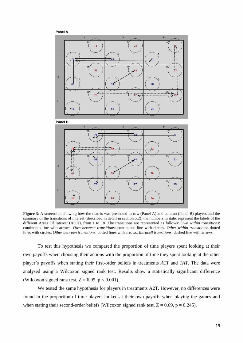
Figure 3: A screenshot showing how the matrix was presented to row (Panel A) and column (Panel B) players and the

summary of the transitions of interest (described in detail in section 5.2); the numbers in italic represent the labels of the

different Areas Of Interest (AOIs), from 1 to 18. The transitions are represented as follows: Own within transitions:

continuous line with arrows. Own between transitions: continuous line with circles. Other within transitions: dotted

lines with circles. Other between transitions: dotted lines with arrows. Intracell transitions: dashed line with arrows.

To test this hypothesis we compared the proportion of time players spent looking at their

own payoffs when choosing their actions with the proportion of time they spent looking at the other

player’s payoffs when stating their first-order beliefs in treatments A1T and 1AT. The data were

analysed using a Wilcoxon signed rank test. Results show a statistically significant difference

(Wilcoxon signed rank test, Z = 6.05, p < 0.001).

We tested the same hypothesis for players in treatments A2T. However, no differences were

found in the proportion of time players looked at their own payoffs when playing the games and

when stating their second-order beliefs (Wilcoxon signed rank test, Z = 0.69, p = 0.245).

20

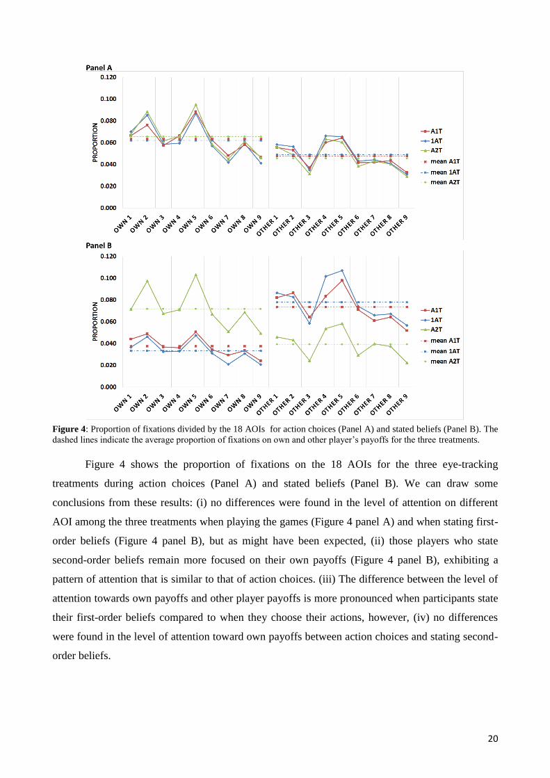
Figure 4: Proportion of fixations divided by the 18 AOIs for action choices (Panel A) and stated beliefs (Panel B). The

dashed lines indicate the average proportion of fixations on own and other player’s payoffs for the three treatments.

Figure 4 shows the proportion of fixations on the 18 AOIs for the three eye-tracking

treatments during action choices (Panel A) and stated beliefs (Panel B). We can draw some

conclusions from these results: (i) no differences were found in the level of attention on different

AOI among the three treatments when playing the games (Figure 4 panel A) and when stating first-

order beliefs (Figure 4 panel B), but as might have been expected, (ii) those players who state

second-order beliefs remain more focused on their own payoffs (Figure 4 panel B), exhibiting a

pattern of attention that is similar to that of action choices. (iii) The difference between the level of

attention towards own payoffs and other player payoffs is more pronounced when participants state

their first-order beliefs compared to when they choose their actions, however, (iv) no differences

were found in the level of attention toward own payoffs between action choices and stating second-

order beliefs.

21

5.3 Definition of the Visual Information acquisition patterns

Following Polonio et al. (2015), we defined the concept of Visual Information Acquisition pattern

(VIA pattern) as the sequence of transitions (a transition is defined as the passage from fixation on

one AOI to another) needed to extract information about the payoff structure of a game.

Considering all possible pairs of AOIs and assuming that each pair can be connected by transitions

(one for each direction), the number of transitions that could be potentially observed equals 324,

including transitions within the same AOI. However, our main objective when analyzing the

transitions was to identify which VIA patterns players used to acquire information about the

structure of the games when facing the 3 by 3 matrices. Therefore, we considered only those

transitions useful to capture pieces of information that are necessary to: 1) identify the presence of

dominant strategies for the player; (2) identify the presence of dominant strategies for the

counterpart; (3) identify the strategy with the highest average payoff among those of the player; (4)

identify the strategy with the highest average payoff among those of the counterpart; (5) compare

the payoffs of both players, within the same cell. The above-mentioned information can be capture

by considering the following five types of transitions, where AOI-own corresponds to the AOIs of

the players’ payoffs (AOIs from 1 to 9 for a row player and from 10 to 18 for a column player), and

AOI-other to those of the counterpart players’ payoffs (AOIs from 10 to 18 for a row player and

from 1 to 9 for a column player):

Own within transitions (Own W): transitions from one AOI-own to another AOI-own, within

the same option of the payoff matrix (e.g., from 1 to 2, or from 1 to 3 for a row player and

from 10 to 13 or from 10 to 16 for a column player). See Figure 3: continuous line with

arrows. Transitions that remain within the same AOI are excluded.

Own between transitions (Own B): transitions from one AOI-own to another AOI-own

between different options (e.g., from 1 to 4, or from 1 to 7 for a row player and from 10 to

11, or from 10 to 12 for a column player). See Figure 3: continuous line with circles.

Transitions that remain within the same AOI are excluded as well as transition that are not

useful to detect dominance (e.g. from 1 to 5, or from 1 to 9 for a row player and from 10 to

14, or from 11 to 18 for a column player).

Other within transitions (Other W): transitions from one AOI-other to another AOI-other,

within the same option of the payoff matrix (e.g., from 12 to 15, or from 12 to 18 for a row

player or from 1 to 2, or from 1 to 3 for a column player). See Figure 3: dotted line with

circles. Transitions that remain within the same AOI are excluded.

22

Other between transitions (Other B): transitions from one AOI-other to another AOI-other,

between different options (e.g., from 16 to 18, or from 17 to 18 for a row player and from 1

to 4 or from 1 to 7 for a column player). See Figure 3, dotted line with arrows. Transitions

that remain within the same AOI are excluded as well as transitions that are not useful to

detect dominance (e.g. from 16 to 15, or from 17 to 12).

Intracell transitions (Intracell): transitions from an AOI-own to an AOI-other or vice versa,

within the same cell (e.g. from 5 to 14). See Figure 3, dashed line with arrows.

From now on, we will refer to these five categories as relevant transitions.

Then, we defined the general VIA patterns that should be used by the players depending on

their types. As mentioned before, we hypothesize that in situations where there is no opportunity to

learn, choice behaviour is driven by 1) motivation, which is concerned with the aims of behavior

and how the human actions are influenced by social motives and 2) cognition, which stands for all

the high-level computational processes like thinking and reasoning. Motivation can drive players'

behavior in different ways, in particular we can distinguish between four different types of social

motives: (a) individualism (attempting to maximize one’s own gain); (b) cooperation or prosocial

behavior (attempting to maximize joint gain); (c) inequity aversion (attempting to minimize the

difference between one’s own gain and others’ gain); and (d) competition (attempting to maximize

the difference between one's own gain and others' gain)17

,

Cognition can be defined as the ability to process information accurately and to implement

adaptive behavior. In a strategic environment, individual differences in cognitive abilities can be

described in terms of different levels of sophistication. This notion concerns the extent to which

players consider the structure of a game and the other players’ incentives before deciding on their

strategy (Crawford et al., 2013). This is especially true in games like the ones we used, which

require at least two steps of iterations to be solved. Costa-Gomes et al. (2001), Bhatt and Camerer

(2005), and Brocas et al. (2014b mimeo) define the pattern of information acquisition employed by

players exhibiting different levels of strategic thinking when playing normal form games. In line

with these studies, we expect sophisticated players to acquire information about the payoffs of their

opponents in order to best respond to their expected actions. To identify equilibrium strategies,

agents can check for dominance or iterated dominance among own and/or other’s decision

strategies, alternatively, they can check directly for pure strategy equilibrium. In both cases own and

other between transitions are expected. A similar VIA pattern is expected from D1 and D2 players

17

There are few empirical evidences supporting a pure altruistic interpersonal orientation in one-shot games, therefore we did not include this model in our analysis.

23

because own between and/or other between transitions are required to check for the presence of

dominated strategies.

L2 players best respond to players who choose the option with the highest average payoff

(L1 players), and therefore they should devote considerable attention to the other player’s payoffs.

More specifically, they are expected to use other within transitions to find the option with the

highest average payoff among the other player’s strategies, and/or other between transitions to

check whether the other player have dominated strategies. Lastly, and before making a decision, we

expect them to use own between transitions in order to choose their best response once the probable

choice of the opponent has been singled out.

Conversely, we expect that less sophisticated players – such as L1, Pessimistic and

Optimistic types – who are not concerned with the opponent’s incentives, remain focused on their

own payoffs without taking into account the payoffs of their counterpart. We expect L1 players to

use own within transitions to calculate the expected value of each strategy or own between

transitions to look for dominance relations. Pessimistic players need to find the option with the

lowest minimum payoff; therefore, we expect them to use own between transitions. Finally,

Optimistic players just need to look their own payoffs to find the highest among them.

EQ, L2, D2, D1, L1, Pess and Opt models retain the assumption of rational self-interest,

whereas Inequity Averse, Prosocial and Competitive types are characterized for having different

motives. In terms of information processing, Inequity Averse players should search for the cell

where the difference between the payoffs of the players is the lowest; Prosocial players should

search for the cell having the highest joint gain; and players who adopt a Competitive decision rule

should search for the option where the overall difference between player’s own and counterpart’s

gain is larger. In each case, players having different motives need to compare the two players’

payoffs within the same cell for all passible game results. Therefore, we expect them to use intracell

transitions.

5.4 Cluster Analysis based on transitions

One of our objectives is to assign each participant to one of our models based on the combination

between action choices and the information search pattern used during the action choice task. To

reach this goal, we grouped participants in clusters based on their proportion of own within payoffs

transitions, own between payoffs transitions, other within payoffs transitions, other between payoffs

transitions and intra-cell transitions. To identify the clusters, we adopted a mixture models cluster

analysis that has extensively been used in studies of game theory and process data (Brocas et al.,

2014a; Devetag et al., 2015; Polonio et al., 2015) and proposed by Fraley and Raftery (2002). The

24

advantage of using this clustering method is that the number of clusters and the clustering criterion

are not determined a priory, but they are optimized by the method itself. Mixture models consider

each cluster like a component probability distribution; then a Bayesian statistical approach is used

to choose between different numbers of clusters and different statistical methods (Fraley and

Raftery, 2002; Fraley et al., 2012). We considered a maximum of nine clusters for up to ten

different models, choosing the combination that maximizes the Bayesian Information Criterion

(BIC). For our data, the BIC was maximized at 1328 by a diagonal model varying volume and

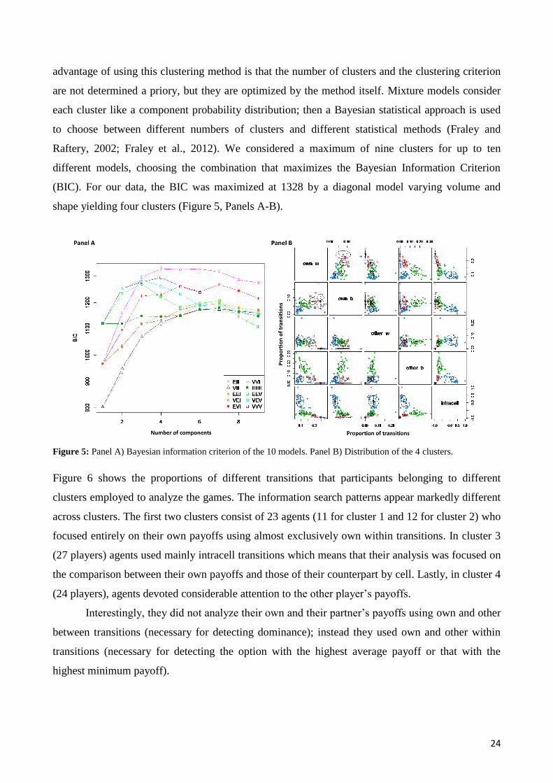
shape yielding four clusters (Figure 5, Panels A-B).

Figure 5: Panel A) Bayesian information criterion of the 10 models. Panel B) Distribution of the 4 clusters.

Figure 6 shows the proportions of different transitions that participants belonging to different

clusters employed to analyze the games. The information search patterns appear markedly different

across clusters. The first two clusters consist of 23 agents (11 for cluster 1 and 12 for cluster 2) who

focused entirely on their own payoffs using almost exclusively own within transitions. In cluster 3

(27 players) agents used mainly intracell transitions which means that their analysis was focused on

the comparison between their own payoffs and those of their counterpart by cell. Lastly, in cluster 4

(24 players), agents devoted considerable attention to the other player’s payoffs.

Interestingly, they did not analyze their own and their partner’s payoffs using own and other

between transitions (necessary for detecting dominance); instead they used own and other within

transitions (necessary for detecting the option with the highest average payoff or that with the

highest minimum payoff).

25

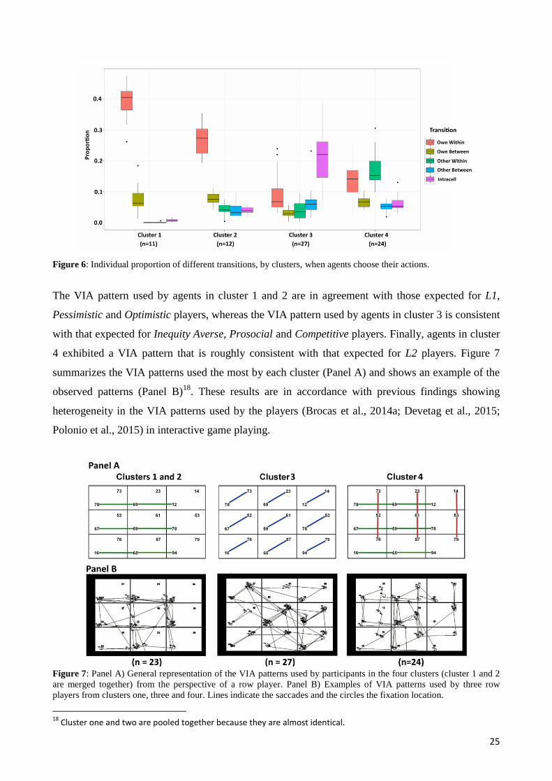
Figure 6: Individual proportion of different transitions, by clusters, when agents choose their actions.

The VIA pattern used by agents in cluster 1 and 2 are in agreement with those expected for L1,

Pessimistic and Optimistic players, whereas the VIA pattern used by agents in cluster 3 is consistent

with that expected for Inequity Averse, Prosocial and Competitive players. Finally, agents in cluster

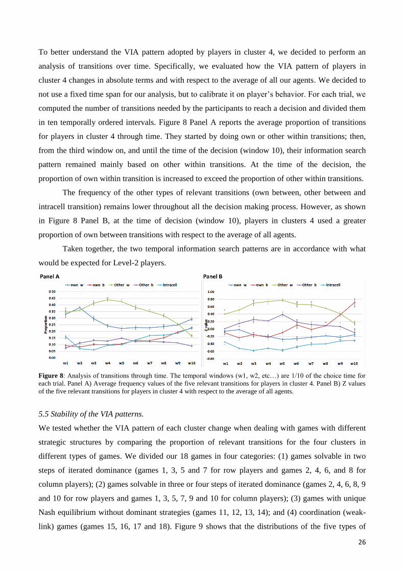
4 exhibited a VIA pattern that is roughly consistent with that expected for L2 players. Figure 7

summarizes the VIA patterns used the most by each cluster (Panel A) and shows an example of the

observed patterns (Panel B)18

. These results are in accordance with previous findings showing

heterogeneity in the VIA patterns used by the players (Brocas et al., 2014a; Devetag et al., 2015;

Polonio et al., 2015) in interactive game playing.

Figure 7: Panel A) General representation of the VIA patterns used by participants in the four clusters (cluster 1 and 2

are merged together) from the perspective of a row player. Panel B) Examples of VIA patterns used by three row

players from clusters one, three and four. Lines indicate the saccades and the circles the fixation location.

18

Cluster one and two are pooled together because they are almost identical.

26

To better understand the VIA pattern adopted by players in cluster 4, we decided to perform an

analysis of transitions over time. Specifically, we evaluated how the VIA pattern of players in

cluster 4 changes in absolute terms and with respect to the average of all our agents. We decided to

not use a fixed time span for our analysis, but to calibrate it on player’s behavior. For each trial, we

computed the number of transitions needed by the participants to reach a decision and divided them

in ten temporally ordered intervals. Figure 8 Panel A reports the average proportion of transitions

for players in cluster 4 through time. They started by doing own or other within transitions; then,

from the third window on, and until the time of the decision (window 10), their information search

pattern remained mainly based on other within transitions. At the time of the decision, the

proportion of own within transition is increased to exceed the proportion of other within transitions.

The frequency of the other types of relevant transitions (own between, other between and

intracell transition) remains lower throughout all the decision making process. However, as shown

in Figure 8 Panel B, at the time of decision (window 10), players in clusters 4 used a greater

proportion of own between transitions with respect to the average of all agents.

Taken together, the two temporal information search patterns are in accordance with what

would be expected for Level-2 players.

Figure 8: Analysis of transitions through time. The temporal windows (w1, w2, etc…) are 1/10 of the choice time for

each trial. Panel A) Average frequency values of the five relevant transitions for players in cluster 4. Panel B) Z values

of the five relevant transitions for players in cluster 4 with respect to the average of all agents.

5.5 Stability of the VIA patterns.

We tested whether the VIA pattern of each cluster change when dealing with games with different

strategic structures by comparing the proportion of relevant transitions for the four clusters in

different types of games. We divided our 18 games in four categories: (1) games solvable in two

steps of iterated dominance (games 1, 3, 5 and 7 for row players and games 2, 4, 6, and 8 for

column players); (2) games solvable in three or four steps of iterated dominance (games 2, 4, 6, 8, 9

and 10 for row players and games 1, 3, 5, 7, 9 and 10 for column players); (3) games with unique

Nash equilibrium without dominant strategies (games 11, 12, 13, 14); and (4) coordination (weak-

link) games (games 15, 16, 17 and 18). Figure 9 shows that the distributions of the five types of

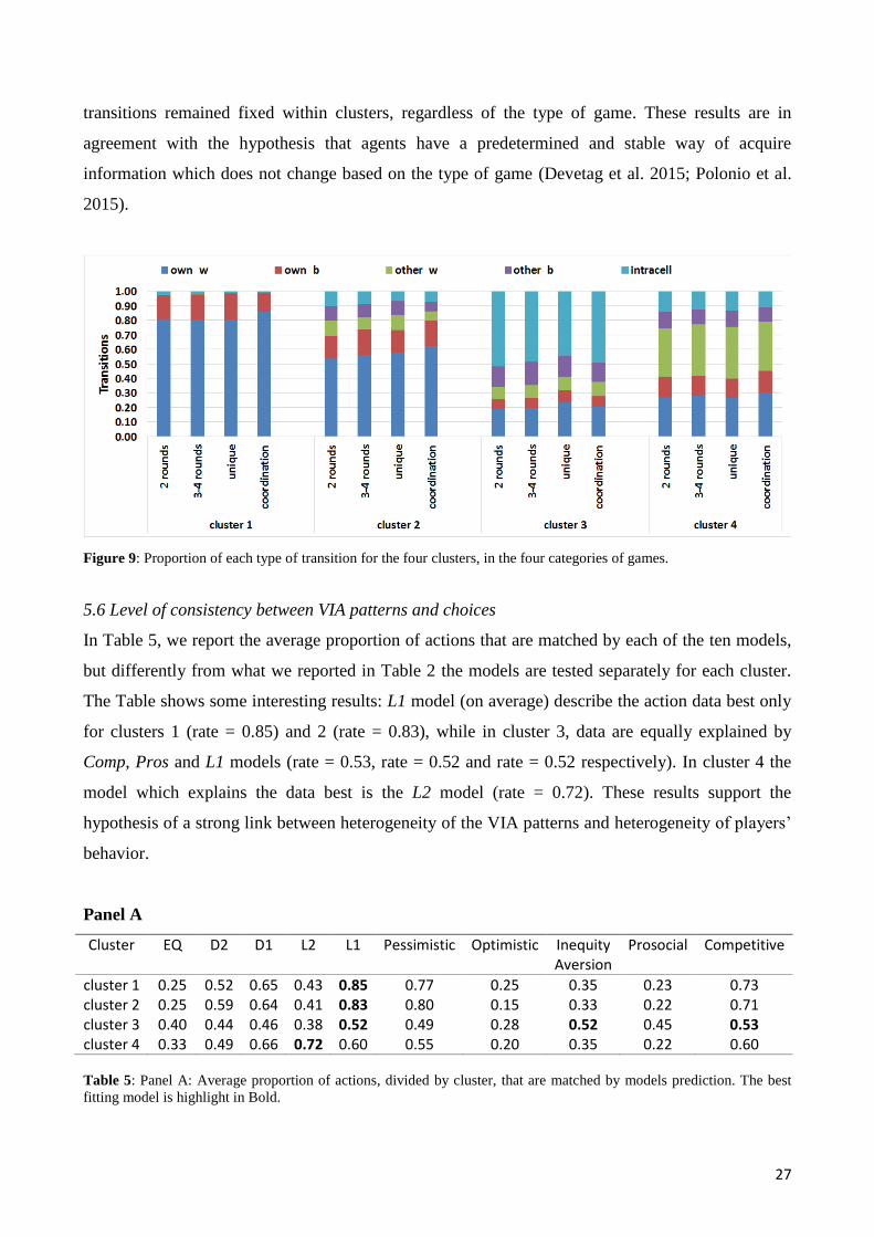
27

transitions remained fixed within clusters, regardless of the type of game. These results are in

agreement with the hypothesis that agents have a predetermined and stable way of acquire

information which does not change based on the type of game (Devetag et al. 2015; Polonio et al.

2015).

Figure 9: Proportion of each type of transition for the four clusters, in the four categories of games.

5.6 Level of consistency between VIA patterns and choices

In Table 5, we report the average proportion of actions that are matched by each of the ten models,

but differently from what we reported in Table 2 the models are tested separately for each cluster.

The Table shows some interesting results: L1 model (on average) describe the action data best only

for clusters 1 (rate = 0.85) and 2 (rate = 0.83), while in cluster 3, data are equally explained by

Comp, Pros and L1 models (rate = 0.53, rate = 0.52 and rate = 0.52 respectively). In cluster 4 the

model which explains the data best is the L2 model (rate = 0.72). These results support the

hypothesis of a strong link between heterogeneity of the VIA patterns and heterogeneity of players’

behavior.

Panel A

Cluster EQ D2 D1 L2 L1 Pessimistic Optimistic Inequity Aversion


cluster 1 0.25 0.52 0.65 0.43 0.85 0.77 0.25 0.35 0.23 0.73 cluster 2 0.25 0.59 0.64 0.41 0.83 0.80 0.15 0.33 0.22 0.71 cluster 3 0.40 0.44 0.46 0.38 0.52 0.49 0.28 0.52 0.45 0.53 cluster 4 0.33 0.49 0.66 0.72 0.60 0.55 0.20 0.35 0.22 0.60

Table 5: Panel A: Average proportion of actions, divided by cluster, that are matched by models prediction. The best

fitting model is highlight in Bold.

28

5.7 Analysis of decisions and information search

To associate each agent to a decision rule we used a procedural view similar to that of Costa-Gomes

et al. (2001), assuming that each type of player defines (with error) her VIA pattern, and her type

and search then jointly determines (again with error) her decision. More specifically, only those

decision models which are compatible with the VIA pattern exhibited by the agent were considered

as possible candidates. Then, each agent was associated with the decision model that best explains

her action choices among the possible candidates.

Equilibrium decisions can be identified by checking directly for pure strategy equilibria or

by best-response dynamics. To check directly for equilibrium (EQ model), own and other between

transitions are required. In dominance solvable games, agents can also use iterated dominance or a

combination of iterated dominance and equilibrium checking. In any case, for equilibrium detection

own and other between transitions are required (Costa-Gomes et al., 2001; Devetag et al., 2015).

Own and other between transitions are also required to check for dominated strategies (D2 and D1

models). However, none of our clusters exhibited a VIA pattern that includes a relevant proportion

of own or other between transitions; therefore, none of our participants were associated to EQ, D2

and D1 players.

In order to best respond to L1 players, L2 players need to collect information about the

payoffs of the counterpart (Costa-Gomes et al., 2001; Bhat and Camerer, 2005; Brocas et al., 2014a;

Devetag et al., 2015; Polonio et al., 2015). In particular, they need to use other within transitions to

look for the strategy giving the counterpart the highest average payoff, or alternatively, other

between transitions to look whether the other player has dominant strategies; then, before making a

decision, they should perform own between transitions to choose a best response to their beliefs.

The VIA pattern exhibited by agents in cluster 4 is compatible to this model.

L1, Pess and Opt models require the players to be focused on own payoffs. Therefore, players in

clusters 1 and 2 can be alternatively associated to one of these three models (Costa-Gomes et al.,

2001; Bhat and Camerer, 2005; Brocas et al., 2014a; Devetag et al., 2015; Polonio et al., 2015).

Inequity Averse, Prosocial and Competitive players need to perform intracell transitions in

order to compare own and other’s payoffs for each possible decision combination (Costa-Gomes et

al., 2001; Devetag et al., 2015; Polonio et al., 2015). Therefore, players in cluster 3 can be

alternatively associated to one of these three models.

To summarize, no agents were classified as EQ, D2 or D1 players. Agents in clusters 1 and

2 were classified as L1, Pessimistic or Optimistic players depending on the model that best explains

their choices. Agents in clusters 3 were classified as Inequity Averse, Prosocial or Competitive

players (again, depending on the model that best explains their choices). Finally, all agents in

29

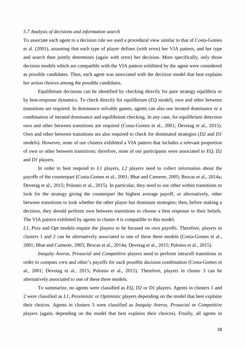
clusters 4 were classified as L2 players. Table 6 shows the number of agents (proportion in

parentheses) assigned to the seven models (L2, L1, Pessimistic, Optimistic, Inequity Aversion,

Prosocial and Competitive) and the average proportion of choices consistent with each model.

Choice consistency Type classification

L2 L1 Pessimistic Optimistic Inequity Aversion Prosocial Competitive

L2 0.72 0.43 0.44 0.22 0.31 0.22 0.48

L1 0.60 0.88 0.81 0.17 0.37 0.33 0.70

Pess. 0.55 0.81 0.89 0.06 0.34 0.25 0.67

Opt. 0.20 0.18 0.03 1.00 0.37 0.44 0.17

IA 0.35 0.34 0.31 0.44 0.69 0.60 0.37

Pros. 0.22 0.22 0.17 0.50 0.59 0.71 0.26

Comp. 0.60 0.75 0.72 0.17 0.36 0.32 0.73

N° of participants (Proportion)

24 (0.32)

20 (0.27)

2 (0.03)

1 (0.01)

10 (0.13)

4 (0.06)

13 (0.18)

Table 6: Proportion of actions in accordance with the seven models by model type, and number (proportion in brackets)

of participants assigned to each type (none of our players were classified as EQ, D2 or D1 types). The best fitting model

is highlight in Bold.

5.8 VIA patterns for the seven models when stating first and second-order beliefs

In this session we test for possible differences between the expected and the observed VIA patterns

used by the agents assigned to the 7 models (L2, L1, Pess, Opt, IA, Pros, Comp), when stating first

and second-order beliefs.

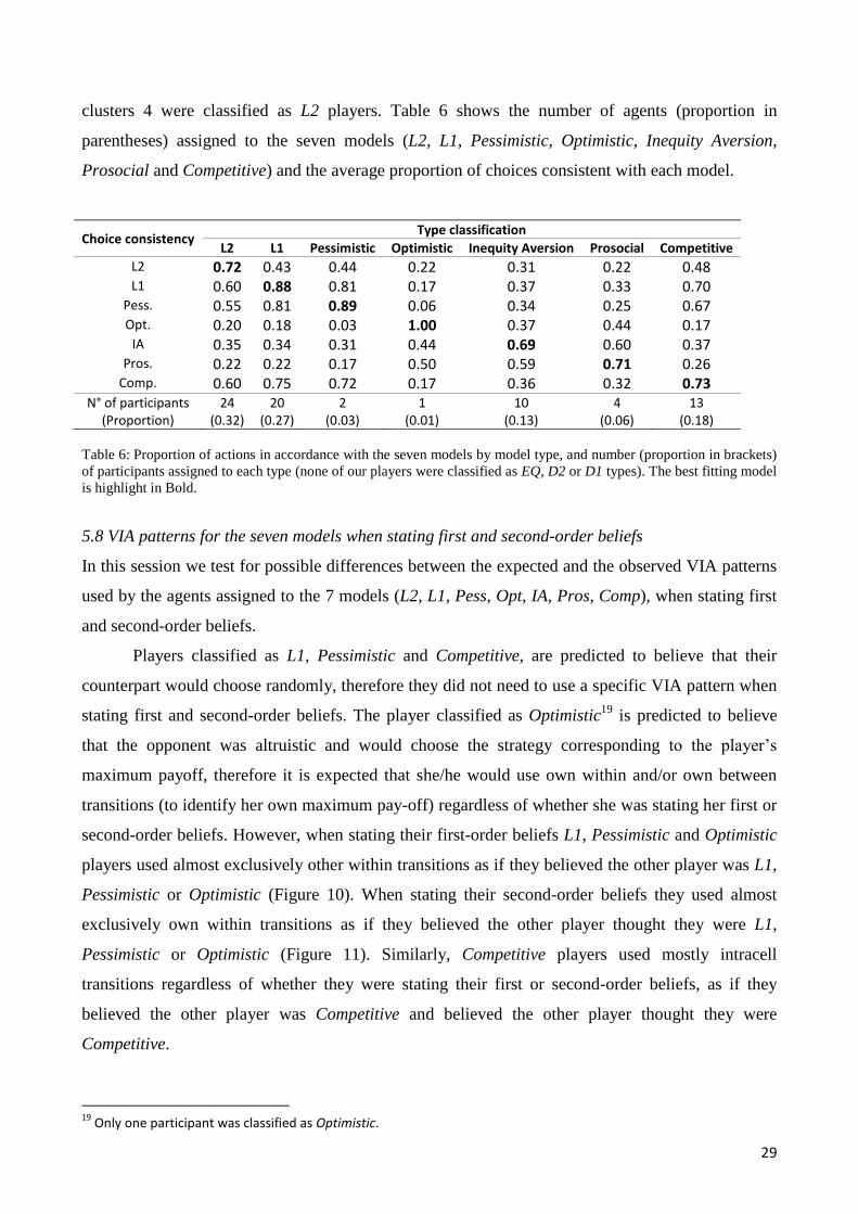
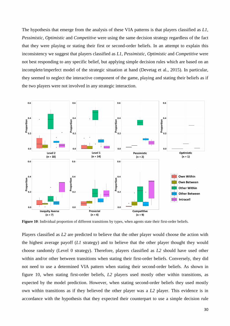
Players classified as L1, Pessimistic and Competitive, are predicted to believe that their

counterpart would choose randomly, therefore they did not need to use a specific VIA pattern when

stating first and second-order beliefs. The player classified as Optimistic19

is predicted to believe

that the opponent was altruistic and would choose the strategy corresponding to the player’s

maximum payoff, therefore it is expected that she/he would use own within and/or own between

transitions (to identify her own maximum pay-off) regardless of whether she was stating her first or

second-order beliefs. However, when stating their first-order beliefs L1, Pessimistic and Optimistic

players used almost exclusively other within transitions as if they believed the other player was L1,

Pessimistic or Optimistic (Figure 10). When stating their second-order beliefs they used almost

exclusively own within transitions as if they believed the other player thought they were L1,

Pessimistic or Optimistic (Figure 11). Similarly, Competitive players used mostly intracell

transitions regardless of whether they were stating their first or second-order beliefs, as if they

believed the other player was Competitive and believed the other player thought they were

Competitive.

19

Only one participant was classified as Optimistic.

30

The hypothesis that emerge from the analysis of these VIA patterns is that players classified as L1,

Pessimistic, Optimistic and Competitive were using the same decision strategy regardless of the fact

that they were playing or stating their first or second-order beliefs. In an attempt to explain this

inconsistency we suggest that players classified as L1, Pessimistic, Optimistic and Competitive were

not best responding to any specific belief, but applying simple decision rules which are based on an

incomplete/imperfect model of the strategic situation at hand (Devetag et al., 2015). In particular,

they seemed to neglect the interactive component of the game, playing and stating their beliefs as if

the two players were not involved in any strategic interaction.

Figure 10: Individual proportion of different transitions by types, when agents state their first-order beliefs.

Players classified as L2 are predicted to believe that the other player would choose the action with

the highest average payoff (L1 strategy) and to believe that the other player thought they would

choose randomly (Level 0 strategy). Therefore, players classified as L2 should have used other

within and/or other between transitions when stating their first-order beliefs. Conversely, they did

not need to use a determined VIA pattern when stating their second-order beliefs. As shown in

figure 10, when stating first-order beliefs, L2 players used mostly other within transitions, as

expected by the model prediction. However, when stating second-order beliefs they used mostly

own within transitions as if they believed the other player was a L2 player. This evidence is in

accordance with the hypothesis that they expected their counterpart to use a simple decision rule

31

(e.g. choosing the option with the highest average payoffs) regardless of the fact that she was

choosing her actions or stating her first-order beliefs.

Players classified as Inequity Averse and Prosocial are predicted to believe that their

counterpart would be cooperative20

and that they believe their counterpart thought they would be

cooperative. Therefore, regardless of the fact that they were stating first or second-order beliefs,

players classified as Inequity Averse and Prosocial should have used intracell transitions. Data in

Figures 10 and 11 show that this prediction is confirmed.

To summarize, from the analyses of the VIA patterns we can make specific predictions

about the expected behavior of the seven types of players when stating first and second-order

beliefs: first, we expect that players classified as L1, Pessimistic, Optimistic and Competitive types

used the same simple decision rules regardless of whether they were choosing their actions or

stating their first or second-order beliefs. Second, we expect that players classified as L2 types

believed that their counterpart would use a simple decision rule (L1 strategy) regardless of whether

she was choosing her actions or stating her first-order beliefs. Third, we expect that players

classified as Inequity Averse/Prosocial types believed their counterpart was Inequity

Averse/Prosocial and thought their counterpart believed they were Inequity Averse/Prosocial.

Figure 11: Individual proportion of different transitions by types when agents state their second-order beliefs.

5.9 Level of consistency between players’ choices and their stated beliefs

In Table 7, we show the proportion of first and second-order beliefs that are in accordance with the

seven models divided by type classification.

Players classified as L2 should have believed that their opponents acted as L1 players; this

prediction is satisfied 86% of the time. Accordingly, we found that players classified as L2 best

responded to their first-order beliefs 71% (SD = 15) of the time (well above the level of chance).

20

Inequity Averse and Prosocial players carry out two different types of cooperative behavior (see session 4). Both types want to coordinate their choices with those of the counterpart but Inequity Averse players want to coordinate on the outcome that minimizes the difference between the payoffs of the two players and Prosocial players want to coordinate on the outcome that maximize the join payoff.

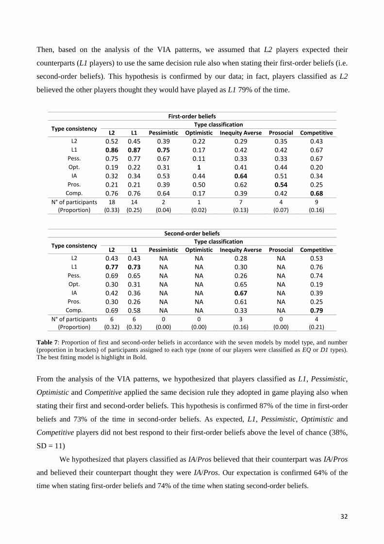
32

Then, based on the analysis of the VIA patterns, we assumed that L2 players expected their

counterparts (L1 players) to use the same decision rule also when stating their first-order beliefs (i.e.

second-order beliefs). This hypothesis is confirmed by our data; in fact, players classified as L2

believed the other players thought they would have played as L1 79% of the time.

First-order beliefs

Type consistency Type classification

L2 L1 Pessimistic Optimistic Inequity Averse Prosocial Competitive

L2 0.52 0.45 0.39 0.22 0.29 0.35 0.43

L1 0.86 0.87 0.75 0.17 0.42 0.42 0.67

Pess. 0.75 0.77 0.67 0.11 0.33 0.33 0.67

Opt. 0.19 0.22 0.31 1 0.41 0.44 0.20

IA 0.32 0.34 0.53 0.44 0.64 0.51 0.34

Pros. 0.21 0.21 0.39 0.50 0.62 0.54 0.25

Comp. 0.76 0.76 0.64 0.17 0.39 0.42 0.68


18 (0.33)

14 (0.25)

2 (0.04)

1 (0.02)

7 (0.13)

4 (0.07)

9 (0.16)

Second-order beliefs

Type consistency Type classification

L2 L1 Pessimistic Optimistic Inequity Averse Prosocial Competitive

L2 0.43 0.43 NA NA 0.28 NA 0.53

L1 0.77 0.73 NA NA 0.30 NA 0.76

Pess. 0.69 0.65 NA NA 0.26 NA 0.74

Opt. 0.30 0.31 NA NA 0.65 NA 0.19

IA 0.42 0.36 NA NA 0.67 NA 0.39

Pros. 0.30 0.26 NA NA 0.61 NA 0.25

Comp. 0.69 0.58 NA NA 0.33 NA 0.79


6 (0.32)

6 (0.32)

0 (0.00)

0 (0.00)

3 (0.16)

0 (0.00)

4 (0.21)

Table 7: Proportion of first and second-order beliefs in accordance with the seven models by model type, and number

(proportion in brackets) of participants assigned to each type (none of our players were classified as EQ or D1 types).

The best fitting model is highlight in Bold.

From the analysis of the VIA patterns, we hypothesized that players classified as L1, Pessimistic,

Optimistic and Competitive applied the same decision rule they adopted in game playing also when

stating their first and second-order beliefs. This hypothesis is confirmed 87% of the time in first-order

beliefs and 73% of the time in second-order beliefs. As expected, L1, Pessimistic, Optimistic and

Competitive players did not best respond to their first-order beliefs above the level of chance (38%,

SD = 11)

We hypothesized that players classified as IA/Pros believed that their counterpart was IA/Pros

and believed their counterpart thought they were IA/Pros. Our expectation is confirmed 64% of the

time when stating first-order beliefs and 74% of the time when stating second-order beliefs.

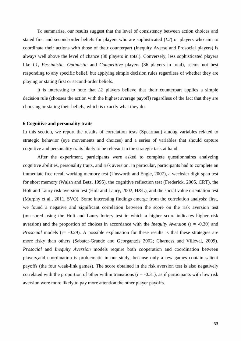
33

To summarize, our results suggest that the level of consistency between action choices and

stated first and second-order beliefs for players who are sophisticated (L2) or players who aim to

coordinate their actions with those of their counterpart (Inequity Averse and Prosocial players) is

always well above the level of chance (38 players in total). Conversely, less sophisticated players

like L1, Pessimistic, Optimistic and Competitive players (36 players in total), seems not best

responding to any specific belief, but applying simple decision rules regardless of whether they are

playing or stating first or second-order beliefs.

It is interesting to note that L2 players believe that their counterpart applies a simple

decision rule (chooses the action with the highest average payoff) regardless of the fact that they are

choosing or stating their beliefs, which is exactly what they do.

6 Cognitive and personality traits

In this section, we report the results of correlation tests (Spearman) among variables related to

strategic behavior (eye movements and choices) and a series of variables that should capture

cognitive and personality traits likely to be relevant in the strategic task at hand.

After the experiment, participants were asked to complete questionnaires analyzing

cognitive abilities, personality traits, and risk aversion. In particular, participants had to complete an

immediate free recall working memory test (Unsworth and Engle, 2007), a wechsler digit span test

for short memory (Walsh and Betz, 1995), the cognitive reflection test (Frederick, 2005, CRT), the

Holt and Laury risk aversion test (Holt and Laury, 2002, H&L), and the social value orientation test

(Murphy et al., 2011, SVO). Some interesting findings emerge from the correlation analysis: first,

we found a negative and significant correlation between the score on the risk aversion test

(measured using the Holt and Laury lottery test in which a higher score indicates higher risk

aversion) and the proportion of choices in accordance with the Inequity Aversion (r = -0.30) and

Prosocial models (r= -0.29). A possible explanation for these results is that these strategies are

more risky than others (Sabater-Grande and Georgantzis 2002; Charness and Villeval, 2009).

Prosocial and Inequity Aversion models require both cooperation and coordination between

players,and coordination is problematic in our study, because only a few games contain salient

payoffs (the four weak-link games). The score obtained in the risk aversion test is also negatively

correlated with the proportion of other within transitions (r = -0.31), as if participants with low risk

aversion were more likely to pay more attention the other player payoffs.

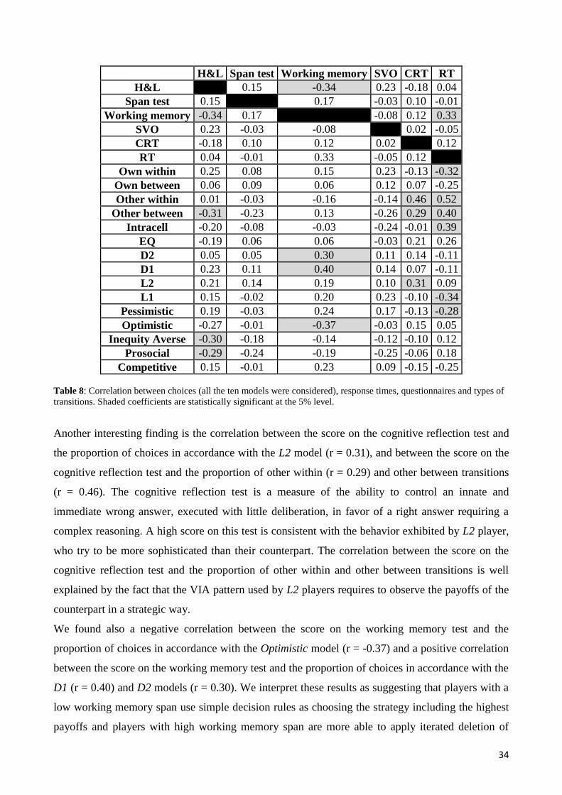
34

H&L Span test Working memory SVO CRT RT

H&L

0.15 -0.34 0.23 -0.18 0.04

Span test 0.15

0.17 -0.03 0.10 -0.01

Working memory -0.34 0.17

-0.08 0.12 0.33

SVO 0.23 -0.03 -0.08

0.02 -0.05

CRT -0.18 0.10 0.12 0.02

0.12

RT 0.04 -0.01 0.33 -0.05 0.12

Own within 0.25 0.08 0.15 0.23 -0.13 -0.32

Own between 0.06 0.09 0.06 0.12 0.07 -0.25

Other within 0.01 -0.03 -0.16 -0.14 0.46 0.52

Other between -0.31 -0.23 0.13 -0.26 0.29 0.40

Intracell -0.20 -0.08 -0.03 -0.24 -0.01 0.39

EQ -0.19 0.06 0.06 -0.03 0.21 0.26

D2 0.05 0.05 0.30 0.11 0.14 -0.11

D1 0.23 0.11 0.40 0.14 0.07 -0.11

L2 0.21 0.14 0.19 0.10 0.31 0.09

L1 0.15 -0.02 0.20 0.23 -0.10 -0.34

Pessimistic 0.19 -0.03 0.24 0.17 -0.13 -0.28

Optimistic -0.27 -0.01 -0.37 -0.03 0.15 0.05

Inequity Averse -0.30 -0.18 -0.14 -0.12 -0.10 0.12

Prosocial -0.29 -0.24 -0.19 -0.25 -0.06 0.18

Competitive 0.15 -0.01 0.23 0.09 -0.15 -0.25

Table 8: Correlation between choices (all the ten models were considered), response times, questionnaires and types of

transitions. Shaded coefficients are statistically significant at the 5% level.

Another interesting finding is the correlation between the score on the cognitive reflection test and

the proportion of choices in accordance with the L2 model (r = 0.31), and between the score on the

cognitive reflection test and the proportion of other within (r = 0.29) and other between transitions

(r = 0.46). The cognitive reflection test is a measure of the ability to control an innate and

immediate wrong answer, executed with little deliberation, in favor of a right answer requiring a

complex reasoning. A high score on this test is consistent with the behavior exhibited by L2 player,

who try to be more sophisticated than their counterpart. The correlation between the score on the

cognitive reflection test and the proportion of other within and other between transitions is well

explained by the fact that the VIA pattern used by L2 players requires to observe the payoffs of the

counterpart in a strategic way.

We found also a negative correlation between the score on the working memory test and the

proportion of choices in accordance with the Optimistic model (r = -0.37) and a positive correlation

between the score on the working memory test and the proportion of choices in accordance with the

D1 (r = 0.40) and D2 models (r = 0.30). We interpret these results as suggesting that players with a

low working memory span use simple decision rules as choosing the strategy including the highest

payoffs and players with high working memory span are more able to apply iterated deletion of

35

dominated strategies. These results, confirm the importance of short-term memory capacity in

strategic reasoning and strategic performance.

Response times (RT) are negatively correlated with the proportion of choices in accordance

with the level-1 model (r = -0.34), as expected considering the low level of complexity of this

model of choices. Moreover, we found positive correlations between RT and other within (r = 0.40),

other between (r = 0.52) and intracell transitions (r = 0.39) and a negative correlation between RT

and own within transitions (r = - 0.32), showing that applying a decision strategy that require a

higher level of sophistication is time demanding. Table 8 reports the correlation coefficients

(correlation coefficients in the shaded cells are significant at the 5 percent level).

7 Conclusions

In this study we report an experiment in which 118 participants played and stated first or second-

order beliefs about their counterparts’ actions in 18 one-shot matrix games. Eye-movements were

recorded for 74 of them. The level of consistency between choices and beliefs is tested by assuming

that participants can be one of several types, and each type may have a different underlying belief

about the counterpart’s strategy. We performed a mixed-model cluster analysis and classified

participants according to their information search patterns. The cluster analysis clearly revealed 3

different types of visual analysis, according to which we categorized players into different types:

one cluster of players was shown to focus prevalently on information regarding their own payoffs,

and they chose accordingly with 3 simple non-strategic models (Level-1, Pessimistic and

Optimistic). A second cluster contained players focused mainly on the comparison between their

own and their counterpart payoffs. They chose accordingly with 3 models of social value

orientation (Inequity averse, Prosocial and Competitive). The third cluster contained players that

exhibited a more balanced mixture of all types of visual analysis, and they chose accordingly with a

sophisticated model (Level-2).

Our results showed that participants have not played according to equilibrium, and neither

they expected their counterpart to do so. However, the level of consistency between action choices

and stated first and second order beliefs for players who were strategically sophisticated (Level-2)

or players who aimed to coordinate their actions with those of their counterpart (Inequity averse and

Prosocial) was always well above the level of chance. Conversely, non-strategic (Level-1,

Pessimistic, Optimistic) and competitive players did not best respond to any specific belief, but

applied simple decision rules regardless of whether they were playing or stating their beliefs.

We found that players categorized as level-2 exhibited a less sophisticated VIA pattern when

stating their first and second order beliefs than when choosing their actions. We also found that

36

Level-2 players believed that the opponent applied a simple decision rule (chose the action with the

highest average payoff) regardless of whether she was choosing her actions or stating her beliefs.

Importantly, we found that this belief was consistent with the behavior exhibited by players

classified as non-sophisticated (Level-1, Pessimistic and Optimistic).

Players classified as non-sophisticated (Level-1, Pessimistic and Optimistic) or Competitive

exhibited the same VIA pattern and used the same decision rules regardless of whether they were

choosing their actions or stating their first or second order beliefs. This is in accordance with the

hypothesis that they were not best responding to any specific belief, but applied simple decision

rules based on an incomplete/imperfect model of the strategic situation at hand (Devetag et al.,

2015). They seemed to neglect the interactive component of the game, playing and stating their

beliefs as if the two players were not involved in any strategic interaction.

Assuming coordination on a mutually advantageous outcome as the objective of Inequity

Averse and Prosocial players, we found consistency between action choices and beliefs also for

players having other-regarding preferences. The VIA pattern exhibited by players classified as

Inequity Averse or Prosocial was characterized by intra-cell saccades between own and other

player’s payoffs regardless of whether they were choosing their actions or stating their first or

second order beliefs. This is exactly the behavior we would expect from players who wanted to

coordinate their actions with those of the counterpart and who believed that the counterpart would

do the same.

Our results have important implications for non-equilibrium models such as level-k

(Crawford, 2003; Nagel, 1995; Stahl and Wilson, 1994, 1995) and Cognitive Hierarchy Models

(CH, Camerer et al., 2004). In a level k model, level-1 best respond to level-0, level-2 to level-1,

and so on. CH model also has a recursive structure but in this case a level-k player best responds not

only to level k-1 but to a mixture of lower-level types. According to these models, we found that

level-2 players best respond to the belief that the opponent is level-1. However, our results show

that level-1 players do not form beliefs at all. Instead, they apply a simple decision rule while

attributing to the opponent their own decision strategy. Our results suggest that strategic players

(level k > 1) anchor their beliefs to an initial assessment of other’s actions corresponding to a level-

1 type instead of a level-0 type.

More generally, our study supports the hypothesis that players’ behavior and stated beliefs,

in one-shot games, are driven by two different types of mental processes: motivation and cognition,

which determined different decision rules or types that remain constant over different games. Our

classification based on the combination of eye-tracking and choice data allows us to accurately

identify the decision rules adopted by the participants, and show an higher level of consistency

37

between choices and stated beliefs compared with previous work (Costa-Gomes and Weizsäcker,

2008; Bhatt and Camerer, 2005).

Finally, we found that part of the heterogeneity observed in players’ behavior can be

explained by differences in risk attitudes, by the ability to control intuitive responses in favor of

reflective and deliberative actions and by the short-term memory capacity.

38

References

Andreoni, J., & Miller, J. (2002). Giving according to GARP: An experimental test of the

consistency of preferences for altruism. Econometrica, 737-753.

Bellemare, C., & Kröger, S. (2007). On representative social capital. European Economic

Review, 51(1), 183-202.

Bhatt, M., & Camerer, C. F. (2005). Self-referential thinking and equilibrium as states of mind in

games: fMRI evidence. Games and Economic Behavior, 52(2), 424-459.

Blanco, M., Engelmann, D., & Normann, H. T. (2011). A within-subject analysis of other-regarding

preferences. Games and Economic Behavior, 72(2), 321-338.

Brocas, I., Carrillo, J. D., Wang, S. W., & Camerer, C. F. (2014a). Imperfect choice or imperfect

attention? Understanding strategic thinking in private information games. Review of

Economic Studies.

Brocas, I., Carrillo, J. D., & Sachdeva, A. (2014b). The Path to Equilibrium in Sequential and

Simultaneous Games. Mimeo.

Camerer, C. F., Ho, T. H., & Chong, J. K. (2004). A cognitive hierarchy model of games. The

Quarterly Journal of Economics, 119(3), 861-898.

Charness, G., & Villeval, M. C. (2009). Cooperation and Competition in Intergenerational

Experiments in the Field and the Laboratory. The American Economic Review, 99(3), 956-

978.

Costa‐Gomes, M., Crawford, V. P., & Broseta, B. (2001). Cognition and Behavior in Normal‐Form

Games: An Experimental Study. Econometrica, 69(5), 1193-1235.

Costa-Gomes, M. A., & Weizsäcker, G. (2008). Stated beliefs and play in normal-form games. The

Review of Economic Studies, 75(3), 729-762.

Crawford, V. P. (2003). Lying for strategic advantage: Rational and boundedly rational

misrepresentation of intentions. American Economic Review, 133-149.

Crawford, V. P., Costa-Gomes, M. A., & Iriberri, N. (2013). Structural models of nonequilibrium

strategic thinking: Theory, evidence, and applications. Journal of Economic

Literature, 51(1), 5-62.

Croson, R. T. A. (2000): Feedback in Voluntary Contribution Mechanisms: An Experiment in Team

Production. Research in Experimental Economics 8, 85-97.

Devetag, G., Di Guida, S., & Polonio, L. (2015). An eye-tracking study of feature-based choice in

one-shot games, forthcoming in Experimental Economics.

Dufwenberg, M., & Gneezy, U. (2000). Measuring beliefs in an experimental lost wallet

game. Games and economic Behavior, 30(2), 163-182.

39

Fehr, E., & Rockenbach, B. (2003). Detrimental effects of sanctions on human altruism. Nature,

422(6928), 137-140.

Fehr, E., & Schmidt, K. M. (1999). A theory of fairness, competition, and cooperation. The

quarterly journal of economics, 114(3), 817-868.

Fisman, R., Kariv, S., and Markovits, D. (2007). Individual Preferences for Giving. American

Economic Review, 97, 1858-1877.

Fraley, C., & Raftery, A. E. (2002). Model-based clustering, discriminant analysis, and density

estimation. Journal of the American Statistical Association, 97(458), 611-631.

Fraley, C., & Raftery, A. E., Murphy, T. B. and Scrucca L., (2012). Normal Mixture Modeling for

Model-Based Clustering, Classification, and Density Estimation. Technical Report No.

597, Department of Statistics, University of Washington.

Frederick, S. (2005). Cognitive reflection and decision making. Journal of Economic perspectives,

25-42.

Goeree, J. K., & Holt, C. A. (2004). A model of noisy introspection. Games and Economic

Behavior, 46(2), 365-382.

Haruvy, E., Stahl, D. O., & Wilson, P. W. (1999). Evidence for optimistic and pessimistic behavior

in normal-form games. Economics Letters, 63(3), 255-259.

Holt, C. A., & Laury, S. K. (2002). Risk Aversion and Incentive Effects. American Economic

Review, 92(5), 1644–1655.

Hung, A., & Dominitz, J. (2004). Homogeneous actions and heterogeneous beliefs: Experimental

evidence on the formation of information cascades. Econometric Society 2004 North

American Winter Meetings (No. 64). Econometric Society.

Iriberri, N., & Rey-Biel, P. (2013). Elicited beliefs and social information in modified dictator

games: what do dictators believe other dictators do.Quantitative Economics, 4(3), 515-547.

Ivanov, A. (2006). Strategic play and risk aversion in one-shot normal-form games: An

experimental study. (Mimeo, Ohio State University).

Manor, B. R., & Gordon, E. (2003). Defining the temporal threshold for ocular fixation in free-

viewing visuocognitive tasks. Journal of neuroscience methods,128(1), 85-93.

Murphy, R. O., Ackermann, K. A., & Handgraaf, M. J. (2011). Measuring social value

orientation. Judgment and Decision Making, 6(8), 771-781.

Nagel, R. (1995). Unraveling in guessing games: An experimental study. American Economic

Review, 85(5), 1313-1326.

Naef, M., and J. Schupp (2008). Measuring Trust: Experiments and Surveys in Contrast and

Combination. Working Paper, Royal Holloway College, London.

40

Nyarko, Y., & Schotter, A. (2002). An experimental study of belief learning using elicited

beliefs. Econometrica, 70(3), 971-1005.

Offerman, T., Sonnemans, J., & Schram, A. (1996). Value orientations, expectations and voluntary

contributions in public goods. The economic journal, 817-845.

Polonio, L., Di Guida, S., Coricelli, G. (2015). Strategic sophistication and attention in games: an

eye-tracking study. ECARES Working Papers.

Rey-Biel, P. (2009). Equilibrium play and best response to (stated) beliefs in normal form

games. Games and Economic Behavior, 65(2), 572-585.

Sabater-Grande, G., & Georgantzis, N. (2002). Accounting for risk aversion in repeated prisoners’

dilemma games: An experimental test. Journal of economic behavior & organization, 48(1),

37-50.

Sapienza, P., Toldra‐Simats, A., & Zingales, L. (2013). Understanding trust. The Economic

Journal, 123(573), 1313-1332.

Stahl, D. O., & Wilson, P. W. (1994). Experimental evidence on players' models of other

players. Journal of economic behavior & organization, 25(3), 309-327.

Stahl, D. O., & Wilson, P. W. (1995). On Players′ Models of Other Players: Theory and

Experimental Evidence. Games and Economic Behavior, 10(1), 218-254.

Unsworth, N., & Engle, R. W. (2007). On the division of short-term and working memory: an

examination of simple and complex span and their relation to higher order

abilities. Psychological bulletin, 133(6), 1038-1066.

Van Lange, P. A., & Liebrand, W. B. (1991). Social value orientation and intelligence: A test of the

goal prescribes rationality principle. European journal of social psychology, 21(4), 273-292.

Van Lange, P. A. (2000). Beyond self-interest: A set of propositions relevant to interpersonal

orientations. European review of social psychology, 11(1), 297-331.

Walsh, W. B., & Betz, N. E. (1995). Tests and assessment . Englewood Cliffs, NJ: Prentice-Hall,

Inc.

Weizsäcker, G. (2003). Ignoring the rationality of others: evidence from experimental normal-form

games. Games and Economic Behavior, 44(1), 145-171.

Documents

Testing the level of consistency between choices and ... · Testing the level of consistency between choices and beliefs in ... Costa-Gomes and ... A low level of consistency between