Testing the Restrictions of the Almon Lag Technique

Testing the Restrictions of the Almon Lag TechniqueAuthor(s): L. G. Godfrey and D. S. PoskittSource: Journal of the American Statistical Association, Vol. 70, No. 349 (Mar., 1975), pp. 105-108Published by: American Statistical AssociationStable URL: http://www.jstor.org/stable/2285384 .

Accessed: 16/06/2014 02:37

Your use of the JSTOR archive indicates your acceptance of the Terms & Conditions of Use, available at .http://www.jstor.org/page/info/about/policies/terms.jsp

.JSTOR is a not-for-profit service that helps scholars, researchers, and students discover, use, and build upon a wide range ofcontent in a trusted digital archive. We use information technology and tools to increase productivity and facilitate new formsof scholarship. For more information about JSTOR, please contact [email protected].

.

American Statistical Association is collaborating with JSTOR to digitize, preserve and extend access to Journalof the American Statistical Association.

http://www.jstor.org

This content downloaded from 188.72.126.55 on Mon, 16 Jun 2014 02:37:24 AMAll use subject to JSTOR Terms and Conditions

http://www.jstor.org/action/showPublisher?publisherCode=astata

http://www.jstor.org/stable/2285384?origin=JSTOR-pdf

http://www.jstor.org/page/info/about/policies/terms.jsp


Testing the Restrictions of the Almon Lag Technique

L. G. GODFREY and D. S. POSKITT*

This article considers testing the restrictions imposed by Almon's approach to estimation of distributed lag relationships. The conventional likelihood ratio test procedure requires that the regression equation be estimated in unrestricted form and then subject to the Almon restrictions. An alternative test is suggested which has the advantage of requiring only that the unrestricted version be estimated. The problem of selecting the order of the polynomial is discussed and a numerical example is presented.

1. INTRODUCTION

Schmidt and Waud [9] have recently considered the polynomial approximation approach to the estimation of distributed lag relationships. This approach was origi- nally suggested by Almon [1] and consists of constraining the lag coefficients to lie on a polynomial. Schmidt and Waud point out that imposing these restrictions when they are false will lead to biased and inconsistent estimates and invalid tests. It is therefore essential to test the acceptability of the Almon restrictions.

The usual approach to testing the restrictions is to fit the unrestricted distributed lag equation and then to fit the imposed Almon structure. The consistency of the restrictions with the sample data is then investigated by applying a likelihood ratio test based on the restricted and unrestricted error sums of squares (see [3, Sect. 8.2, pp. 227-9]).

This article outlines a test based only on the least squares estimates of the unrestricted distributed lag equation, so that the acceptability of the polynomial restrictions can be assessed without actually using Almon's estimation method. The procedure of this note therefore permits the testing of various alternative orders of polynomials without incurring the cost of estimating the corresponding restricted lag models, as required by the likelihood ratio approach. It follows that this test will be especially useful when the investigator does not know the order of the polynomial and has to search for an acceptable value.' The problem of selecting the order of the polynomial is discussed and a numerical

* L.G. Godfrey and D.S. Poskitt are lecturers, Department of Economics and Related Studies, University of York, Heslington, York Y01 5DD, England. The authors are grateful to R.A. Cooper, J.P. Hutton, a referee and an associate editor for helpful comments.

1 The use of the likelihood ratio test procedure in this situation would require that the investigator undertake the unnecessary burden of estimating each of the Almon models to be considered. The additional cost of the likelihood ratio approach is especially high if the Almon model is based on the Lagrangian polynomials rather than the simple polynomials.

example is presented to illustrate the test procedure described here.

2. THE MODEL

Consider the simple distributed lag model'

Yt = Xtwo + Xt_1W1 + * *-- + xtw + ut, (2.1)

where yt is the value of the dependent variable in period t, xti is the value of the exogenous variable x in period (t - i), and the ut are assumed to be independently normally distributed with mean zero and variance 72. It is assumed that T observations are available on (2.1).

The Almon polynomial approach is to restrict the lag coefficients wi to lie on a polynomial of order p, i.e.,

W = +X1jjXli + X2 +- + XjP,p

(i = O, n), p < n . (2.2)

These restrictions reduce the number of coefficients to be estimated from (n + 1) to (p + 1). If p equals n, then no restrictions are imposed since it is always possible to find a polynomial of order n passing through (n + 1) specified points in Eudlidean 2-space. In the no restrictions case, (2.2) can be expressed in matrix-vector form as

w = Al (2.3)

where w' = (wo, wi, * *, W Z) It = (Xo, X1, ..., IX n) and A is an (n + 1) by (n + 1) nonsingular matrix with typical element

a= iJ (i,j= O 1, * n)

It will be useful to rewrite (2.3) as

2= Bw, (B = A-'). (2.4)

3. THE TEST PROCEDURE

The testing of a typical set of Almon restrictions is now considered, and the null hypothesis is that the wi coefficients lie on a polynomial of order p, (p < n). The following partitions of A, B and X will be required:

A = (Ap+?: A1p+) y

2 The value of n is assumed to have been known or determined by the researcher. Malinvaud [6, pp. 580-2], and Schmidt and Waud [9, pp. 12-3], have discussed the problem of selecting the length of the lag.

? Journal of the American Statistical Association March 1975, Volume 70, Number 349

Theory and Methods Section

105



106 Journal of the American Statistical Association, March 1975

where A,+, is (n + 1) by (p + 1) and A,+, is (n + 1) by (n -p);

B' = ((Bp+i'): (Bp+i'))I

where BP+1 is (p + 1) by (n + 1) and Rp+j is (n - p) by (n + 1); and

it = ((1p+l ): (1p+l )) I

where lp+l is (p + 1) by 1 and 4p+1 is (n - p) by 1.

Equation (2.4) can therefore be written as

1p+l = BP+w+ , (2.4a) and

1P+ = BP+1w. (2.4b)

Under the null hypothesis that the coefficients of the distributed lag model (2.1) lie on a polynomial of order p, the vector lp+i has every element equal to zero. The Almon technique, therefore, implies the coefficient restrictions

O = P+1w, (3.1)

where flB1 is a matrix of known constants. The test procedure of this note is essentially a test of

the hypothesis embodied in (3.1) and will be based only on simple least squares estimation of the unrestricted model (2.1). The matrix-vector representation of the basic model will be taken as

y = Xw?u, (3.2)

where y is a T by 1 vector of observations on the dependent variable, X is a T by (n + 1) matrix of observations on the regressors, and u is a T by 1 vector of residuals. The Almon distributed lag model associated with the restrictions represented by (3.1) is

y = XAp+lAp+l + u = X> +11p+1 + u , where X*+1 = XAp+l. (3.2a)

The unrestricted least squares estimator of the vector of lag coefficients is

* = (X'X)-lX'y , (3.3)

which is normally distributed with mean vector w and variance-covariance matrix r2 (X'X)-l. In practice, o-2 will be unknown and estimated by S2 which is defined by

S2 = (y - Xw)'(y - Xw')/(T - n - 1) . (3.5)

The estimated variance-covariance matrix of 'w is denoted by

V = s2(X'X)-1 (3.6)

The hypothesis that the Almon restrictions are valid can then be tested by calculating

F = (Bp+i w)'(Rp+,V(Rp+,'))-1(lRp+, w)/(n -p), (3.7)

which is distributed as iFn-p,T-n-1 under the null hypothesis (see [7, Sect. 4b.2, pp. 196-7]). Significantly high values of F imply that the polynomial restrictions

are not consistent with the sample data and should not be applied.3

It is straightforward to show that the test statistic defined by (3.7) is equal to the likelihood ratio test statistic

FLR = (ESS (-p+) - ESS (W))/s2 (n - p),

where ESS ( w) and ESS ("p+') are the error sums of squares associated with the least squares estimation of (3.2) and (3.2.a), respectively. It follows that the test procedure suggested above yields the likelihood ratio test without the cost of estimating the Almon model (3.2.a). This saving will be especially important in the usual case when the degree of the polynomial is unknown and so the researcher has to experiment with different values of p. Since the test of this note is equal to the likelihood ratio test, it has the optimum properties described by Kendall and Stuart [5, pp. 265-6].

The test procedure is then:

(a) estimate the unrestricted equation to obtain 'w and V; (b) obtain B, the inverse of the matrix A; (c) for each value of p to be considered, compute F according

to (3.7) and compare the sample values to the critical values for prespecified levels of significance and appropriate degrees of freedom parameters.

If an acceptable value of p can be found, then the Almon lag technique can be applied.

The calculation of the matrix B, the inverse of the matrix A, is clearly an important part of the test procedure. The matrix A is a Vandermonde matrix, and its determinant is equal to n!(n - 1)!... 1!. The magnitude of its determinant for moderate values of n suggests that direct inversion using standard methods may pose computational problems. Fortunately, it is not necessary to invert the matrix A to obtain the elements of the matrix B. Consider the Lagrangian polynomials

Xi(Z) = Hi (z)/i (zi,), (i = 0, 1 *, n) where

Hi (z) = (Z-Zo)(Z-Z )-

(z - zi-1)(z - zi+1) ... (z - Zn)

and zi i, (i = , 1, ,n). Let

Xi(Z)= c cjzi, (i,j = 0,1, *, n) . (3.8) i

It is clear that

i(ji) = bij, where Sij is the Kronecker delta (i, j = 0, l, , n)

so that the coefficients (coi, cii, ***, C,j) of the Lagrangian polynomials of (3.8) are the elements of the ith column of the matrix B. The coefficients of these polynomials can be readily evaluated.4

3 The distribution of the test statistic under the alternative hypothesis is non- central <i-p T_n_l with noncentrality parameter equal to

4 A set of FORTRAN IV subroutines have been programmed to compute the inverse of A and the F-statistic. Listings will be available on request.



Testing Almon Restrictions 107

Finally, it seems likely that the basic econometric model (2.1) will include variables other than current and lagged values of the variable x, so that, in general, the relationship will be of the form

y = Xw + Zd + u (3.9)

where Z is a T by m matrix of exogenous variables and d is an m size vector of regression coefficients. The only change to the practical implementation of the F-test implied by this modification of the model is that the F statistic now has the 5;n-p,T-.-1-m distribution. The error variance estimator S2 and V, the variance-covariance matrix of the *r subset of the least squares estimators, are, of course, no longer given by (3.5) and (3.6).

4. DETERMINING THE DEGREE OF THE ALMON POLYNOMIAL

This section discusses the application of the test just proposed to the problem of determining the degree of the Almon polynomial. The null hypothesis considered in Section 3 is that the polynomial is of degree less than or equal to p, given that its degree can be at most n. In empirical investigations, however, the researcher will not know the degree of the Almon polynomial and will want to select the most appropriate degree within some range of possibilities and not merely to test whether the polynomial should be of some specified order or less. It will therefore be assumed that there is some number r(r > 0) which is the lowest possible degree and some maximum degree s(s < n), and the problem is to decide whether the polynomial is of degree r, r + 1, , s - 1, or s. It will be assumed in the following that there is no a priori information available about r and s, so that the researcher sets r equal to zero and s equal to n.

Formally, the investigator is faced by the following set of hypotheses:

H.: xn = 0 Hn-1 XwnI= n= 0

Hi: Xi = )iur1 = X* * = )n = ? (4.1)

Hi: Xi = )2 = *=n = O .

The hypotheses are nested in the sense that if any hypothesis of (4.1) is true, the preceding hypotheses must be true, and if any hypothesis is false, then the succeed- ing ones must also be false, i.e., H1 C ... C Hn. The null hypotheses become more and more stringent, forming an increasingly finer partition of the parameter space (X1, * * *, Xn). Thus, for this multiple decision problem, a statistical procedure is required consisting of a set of n regions in the sample space S = (w, V), denoted by Ri, .. *, Rn, such that if the sample falls in Ri, then the hypothesis Hi is accepted and R1 C* * C Rn.

The test proposed in the foregoing is a member of the class of consistent variance ratio tests, and the results of Saw [8] imply that the UMP critical region for testing

Hi at critical level ei is given by Wi consisting of (W, V) satisfying

(Ri W") (iV(Bi'))-l V /(n - i + 1) > Fi* , (4.2)

where Fi* is chosen so that the probability of a random variable which has the central 5Y distribution with parameters n - i + 1 and T - n - 1 exceeding Fi* is i. Thus, the optimal procedure for a given Type I error -i is to select Ri = Wi, the complement of Wi, thereby minimizing the probabilities of deciding that the coefficients are zero when they are not and so using too low a degree for the Almon polynomial.

As the hypotheses form an increasingly finer partition of the parameter space, the Type I risks E, should form a monotonically nondecreasing sequence since the probability of rejecting a more restrictive null hypothesis when it is true must be at least as great as that of rejecting a less restrictive null hypothesis when it is true. Consider therefore the selection of Ei = Pr (Wi Hi), i = n, n-1, * 1.

Suppose that the investigator controls directly the probability of choosing a higher degree polynomial than is necessary and that he wishes to ensure that

Pr (R,I I Hn) = (1 - a)

and

Pr (Ri I Ri+l, Hi) = (1- a) i-n -1, n- 2, , 1 .(4.3)

The procedure represented by (4.3) was suggested by Anderson [2] in the context of choosing the degree of a polynomial regression.5 The investigator is assumed to test Hn, then to test Hn-1 if Hn is accepted and so on until some Hi is rejected. Equation (4.3) implies that the 'conditional' Type I error is constant, so that the probability of deciding that the polynomial is of degree i when it is actually less is independent of i. The un- conditioned Type I errors Ei can be obtained from (4.3) since

Pr (Ri f Hi) = (1-Ei) = Pr (Ri I Ri+1, Hi) * Pr (Ri+i I Hi) = (1 -a) Pr (Ri+iI Hi) I

and it is easily verified that the Type I errors are given by6

et = 1 - (1 - a)n-i+1 , {i = n, n -1, ... 11 .

The choice of a, and hence of ei, will in part be determined by the investigator's attitude to overstating the degree of the polynomial. The statistical cost of employing too high a degree is that there will be a loss of efficiency, although the Almon estimators will still be consistent and unbiased. The use of too low a degree will

5 The problem investigated by Anderson is similar in construction and solution to the one examined in this section. Dhrymes [3, Sect. 11.1, pp. 326-9], has considered Anderson's method of analysis in a discussion of tests on the parameters of the rational distributed lag model.

6 A table of Ei values for conventional values of a will be available from the authors.



108 Journal of the American Statistical Association, March 1975

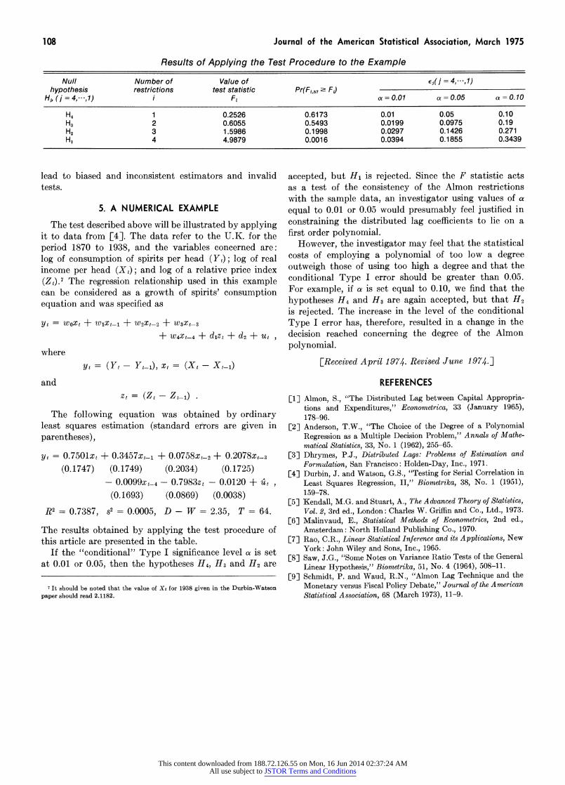
Results of Applying the Test Procedure to the Example

Null Number of Value of Ej(j = 4,---,l) hypothesis restrictions test statistic Pr(Fi,57 ? FJ

Hj, ( j = 4,-. -, 1) i Fi ac= 0.01 a = 0.05 a = 0.10

H4 1 0.2526 0.6173 0.01 0.05 0.10 H3 2 0.6055 0.5493 0.0199 0.0975 0.19 H2 3 1.5986 0.1998 0.0297 0.1426 0.271 H1 4 4.9879 0.0016 0.0394 0.1855 0.3439

lead to biased and inconsistent estimators and invalid tests.

5. A NUMERICAL EXAMPLE

The test described above will be illustrated by applying it to data from [4]. The data refer to the U.K. for the period 1870 to 1938, and the variables concerned are: log of consumption of spirits per head (Yt); log of real income per head (Xt); and log of a relative price index (Zt).7 The regression relationship used in this example can be considered as a growth of spirits' consurn'ption equation and was specified as

Yt = WOXt + WlXtil + W2X,_2 + W3Xt-3

+ W4Xt4 + dlzt + d2 + Ut

where yt = (Yt - Yt_1), xt = (Xt -xt_)

and Zt = (Zt- Zt-_)

The following equation was obtained by ordinary least squares estimation (standard errors are given in parentheses),

yt = 0.7501xt + 0.3457xt1- + 0.0758xt-2 + 0.2078xt-3 (0.1747) (0.1749) (0.2034) (0.1725)

- 0.0099xt4 - 0.7983zt - 0.0120 + u (0.1693) (0.0869) (0.0038)

R' = 0.7387, s2 = 0.0005, D - W = 2.35, T = 64.

The results obtained by applying the test procedure of this article are presented in the table.

If the "conditional" Type I significance level a is set at 0.01 or 0.05, then the hypotheses H4, H3 and H2 are

7 It should be noted that the value of Xt for 1938 given in the Durbin-Watson paper should read 2.1182.

accepted, but H1 is rejected. Since the F statistic acts as a test of the consistency of the Almon restrictions with the sample data, an investigator using values of a equal to 0.01 or 0.05 would presumably feel justified in constraining the distributed lag coefficients to lie on a first order polynomial.

However, the investigator may feel that the statistical costs of employing a polynomial of too low a degree outweigh those of using too high a degree and that the conditional Type I error should be greater than 0.05. For example, if a is set equal to 0.10, we find that the hypotheses H4 and H3 are again accepted, but that H2 is rejected. The increase in the level of the conditional Type I error has, therefore, resulted in a change in the decision reached concerning the degree of the Almon polynomial.

EReceived April 1974. Revised June 1974.]

REFERENCES

[1] Almon, S., "The Distributed Lag between Capital Appropria- tions and Expenditures," Econometrica, 33 (January 1965), 178-96.

[2] Anderson, T.W., "The Choice of the Degree of a Polynomial Regression as a Multiple Decision Problem," Annals of Mathe- matical Statistics, 33, No. 1 (1962), 255-65.

[3] Dhrymes, P.J., Distributed Lags: Problems of Estimation and Formulation, San Francisco: Holden-Day, Inc., 1971.

[4] Durbin, J. and Watson, G.S., "Testing for Serial Correlation in Least Squares Regression, II," Biometrika, 38, No. 1 (1951), 159-78.

[5] Kendall, M.G. and Stuart, A., The Advanced Theory of Statistics, Vol. 2, 3rd ed., London: Charles W. Griffin and Co., Ltd., 1973.

[6] Malinvaud, E., Statistical Methods of Econometrics, 2nd ed., Amsterdam: North Holland Publishing Co., 1970.

[7] Rao, C.R., Linear Statistical Inference and its Applications, New York: John Wiley and Sons, Inc., 1965.

[8] Saw, J.G., "Some Notes on Variance Ratio Tests of the General Linear Hypothesis," Biometrika, 51, No. 4 (1964), 508-11.

[9] Schmidt, P. and Waud, R.N., "Almon Lag Technique and the Monetary versus Fiscal Policy Debate," Journal of the American Statistical Association, 68 (March 1973), 11-9.



Documents

Testing the Restrictions of the Almon Lag Technique