( '

I I

( I

( I

I I

( I

I I

I }

I I

I I

\ I

( I

TESTS OF DISTRIBUTIONAL ASSUMPTIONS AND THE INFORMATIONAL CONTENT OF AGRICULTURAL FUTURES OPTIONS

by

Lee Ziegler

A thesis submitted in partial fulfillment of the requirements for the degree

of

Master of Science

m

Applied Economics

MONTANA STATE UNNERSITY-BOZEMAN Bozeman, Montana

May 1997

I l

! '

I I

( i

I I

( I

I I

I I

I I

I I

I I

11

APPROVAL

of a thesis submitted by

Lee Ziegler

Tins thesis has been read by each member of the thesis committee and has been found to be satisfactory regarding content, English usage, format, citations, bibliographic style, and consistency, and is ready for subnlission to the College of Graduate Studies.

David Buschena (Signature) Date

Approved for the Department of Agricultural Economics and Economics

Myles Watts (Signature) Date

Approved for the College of Graduate Studies

Robert Brown (Signature) Date

( I

I I

I I

I I

I I

I '

I I

I 1

( I

I I

I I

( I

111

STATEMENT OF PERMISSION TO USE

In presenting this thesis in partial fulfilhnent of the requirements for a master's

degree at Montana State University-Bozeman, I agree that the Library shall make it

available to bonowers under rules of the Library.

If I have indicated my intention to copyright this thesis by including a copyright

notice page, copying is allowable only for scholarly purposes, consistent with "fair use"

as prescribed in the U.S. Copyright Law. Requests for pennission for extended quotation

fi:om or reproduction of tllis thesis in whole or in parts may be granted only by the

copyright holder.

Signature------------

Dme __________________ _

(

I I

I I

I I

I I

I I

I I

I I

I I

I I

IV

VITA

Lee Zachary Ziegler was bom in Billings, Montana on Febmary 25, 1973 and is the son of Leighton and Karen Ziegler. He grew up in Sidney, Montana, where he attended school, receiving his high school diploma in May, 1991. He graduated from Rocky Mountain College in May, 1995, where he eamed degrees in mathematics and economics. He began graduate study in applied economics at Montana State University in August, 1995, and received his master of science degree in May of 1997.

( '

i '

I I

I I

( '

I I

( I

I i

( '

v

ACKNOWLEDGMENTS

I would like to thank my graduate committee chair, Dr. David Buschena. Without

his help this thesis would never have been completed. I would also like to thank the other

members of my committee: Professor Joe Atwood, who suggested the use of the Fortran

search procedure to find implied volatilities; Myles Watts, whose insight helped me

develop a better understanding of the various econometric techniques used throughout in

this thesis; and Alan Baquet, who helped provide the futures and options data used in this

thesis. I also wish to aclmowledge my two major undergraduate advisors, Bill Jamison,

Professor of mathematics, and Bernard Rose, Professor of economics, both of Rocky

Mountain College in Billings, Montana. They were nonetheless an important part of my

successful completion of graduate school.

Finally, I wish to thruuc Jan Chavosta, Sheila Smith, and Julie Seru·le for their

computer and editorial assistance in the completion of tlus thesis.

Vl

TABLE OF CONTENTS

Page

INTRODUCTION...................................................................................................... 1

LITERATURE REVIEW AND MODEL LAYOUT................................................. 5

An Overview of Futures and Options Markets.................................................... 5 ( I Potential Infmmational Content of Agricultural Futures Options Market.. ......... 13 ( ' Modeling Futures Price Movements .................................................................... 15

The Lognormal Distribution of Futures Plices .................................................... 17 Framework for Empirical Model. ........................................................................ 19 Option P1icing Models ......................................................................................... 21 The Black-Scholes Parameters ............................................................................. 25 Seasonality of Futures Price Volatility ................................................................. 30 A Method for Testing the Informational Content ofimplied Volatility ............... 32 Description of the Data .......................................................................................... 41

I ' EMPIRICAL RESULTS .............................................................................................. 45

Histmical Futures Price Standard Deviation ........................................................ .45

( ' Futures Price as Unbiased Mean Estimate ............................................................ 50 Futures Price Lognormality ................................................................................... 57 linplied Volatility .................................................................................................. 66 linplied Standard Deviation .................................................................................. 7 4 Relationship Between Put and Calllinplied Volatilities ...................................... 81 Levels of linplied Volatilities and Price Changes ................................................. 82 OLS Estimation ..................................................................................................... 95 Heteroskedasticity ................................................................................................ 1 04

CONCLUSIONS......................................................................................................... 111

Smnmary ofResults ............................................................................................. 111 Implications .......................................................................................................... 113

LITERATURE CITED ............................................................................................... 116

APPENDIX ................................................................................................................. 118

vii

LIST OF TABLES

Page

Table 1: Payoffs From Fom Basic Options Positions ........................................................ 11

Table 2: Monthly Futmes Price Log-Change Standard Deviation, December Com Futmes .................................................................................................................. 47

Table 3: Monthly Futures Price Log-Change Standard Deviation, November CBOT Soybeans .............................................................................................................. 48

Table 4: Monthly Futmes Price Log-Change Standard Deviation, September CBOT Spring Wl1eat. ...................................................................................................... 49

I I

Table 5: Futmes Price Unbiased Estimate Test for Com, OLS Test.. ............................... 52

Table 6: Futmes Price Unbiased Estimate Test for Soybeans, OLS Test.. ........................ 53

Table 7: Futmes Price Unbiased Estimate Test for Spring Wl1eat, OLS Test.. ................. 53

I ' Table 8: Futmes Price Unbiased Estimate Test for Com, Soybeans, and Spring Wlleat: Restrictions Test. ..................................................................................... 56

Table 9: Lognonnality Tests for December CBOT Com Futmes Prices .......................... 60

Table 10: Lognonnality Tests for November CBOT Soybean Futmes Prices .................. 62

Table 11: Lognonnality Tests for September Spring W11eat Futmes Prices ..................... 64

Table 12: Volatilities Implied in December CBOT Com Call Futmes Options P1ices ..... 68

Table 13: Volatilities Implied in December CBOT Com Put Futures Options Prices ...... 69

Table 14: Volatilities Implied in November CBOT Soybean Call Futmes Options Prices .................................................................................................... 70

Table 15: Volatilities Implied in November CBOT Soybean Put Futmes Options Plices .................................................................................................... 71

V111

LIST OF TABLES-Continued

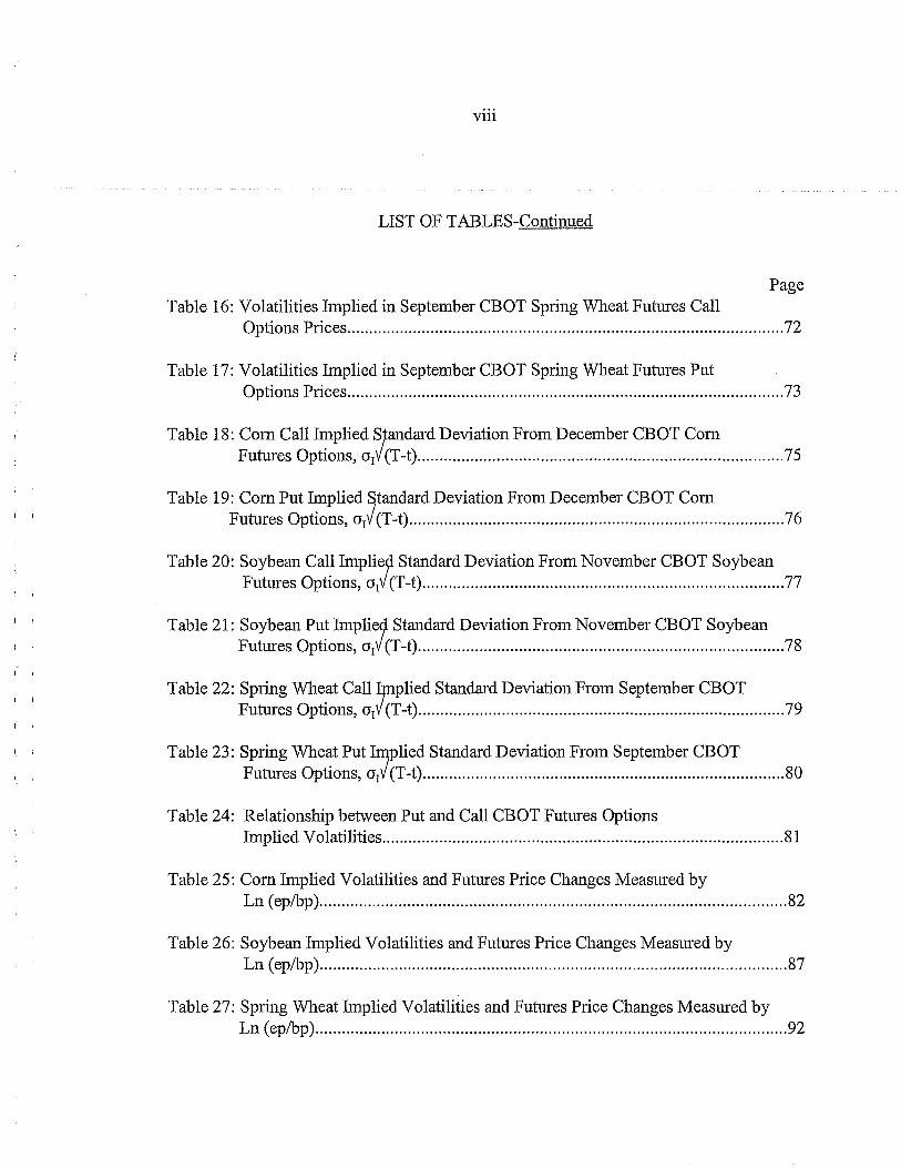
Page Table 16: Volatilities Implied in September CBOT Spring Wheat Futures Call

Options Prices ................................................................................................... 72

Table 17: Volatilities hnplied in September CBOT Spring Wheat Futures Put Options Prices ................................................................................................... 73

Table 18: Com Call Implied Standard Deviation From December CBOT Com Futures Options, a1V(T-t) ................................................................................... 75

I I

Table 19: Com Put hnplied Standard Deviation From December CBOT Com Futures Options, a1V(T-t) ..................................................................................... 76

I I

I I

Table 24: Relationship between Put and Call CBOT Futures Options Implied Volatilities ........................................................................................... 81

Table 25: Com Implied Volatilities and Futures Price Changes Measured by Ln (ep/bp) .......................................................................................................... 82

Table 26: Soybean Implied Volatilities and Futures Price Changes Measured by Ln (ep/bp) .......................................................................................................... 87

Table 27: Sp1ing Wheat hnplied Volatilities and Futures Price Changes Measured by Ln (ep/bp) ........................................................................................................... 92

IX

LIST OF TABLES-Continued Page

Table 28: OLS Results for Ln (ep/bp) on Corn Call hnplied Volatility ................. :··········98

Table 29: OLS Results for Ln (ep/bp) on Corn Put hnplied Volatility ............................ 99

Table 30: OLS Results for Ln (ep/bp) on Soybean Call hnplied Volatility ................... 100

( I Table 31: OLS Results for Ln (ep/bp) on Soybean Put hnplied Volatility ..................... 101

Table 32: OLS Results for Ln (ep/bp) on Spring Wheat Call hnplied Volatility ........... 101

Table 33: OLS Results for Ln (ep/bp) on Spring Wheat Put hnplied Volatility ............ 102 ( I

Table 34: Heteroskedasticity for Corn, Ln ( ep/bp) on hnplied Volatility ...................... 1 07

Table 35: Heteroskedasticity for Soybeans, Ln(ep/bp) on hnplied Volatility ................ 108

Table 36: Heteroskedasticity for Spring wheat, Ln(ep/bp) on hnplied Volatility .......... 109 \ I

I I Table 3 7: Sample Size for Corn Call Futures Options hnplied Volatilities ................. 119

( I

Table 3 8: Sample Size for Corn Put Futures Options hnplied Volatilities .................... 119 ~ I

Table 39: Sample Size for Soybean Call Futures Options hnplied Volatilities ............. l20

Table 40: Sample Size for Soybean Put Futures Options hnplied Volatilities .............. 120

Table 41: Sample Size for Spring Wheat Call Futures Options hnplied Volatilities .... 121

Table 42: Sample Size for Spring Wheat Put Futures Options hnplied Volatilities ...... 121

( '

I I

I I

( I

I I

I I

I I

X

ABSTRACT

It has been proposed that agricultural futures options contain information which may be used by those involved in agriculture, such as rate setting for crop (revenue) insurance. Specifically, it is proposed that these options may be used to predict the variance and perhaps higher moments of the distribution of the respective futures prices. This thesis first tests distributional assumptions maintained by the Black-Scholes analysis. It is found that many ofthese assumptions, such as the commonly used lognormality, are empirically rejected. FJ.rrthermore, it is found that futures price change standard deviations and futures options implied volatilities display seasonal patterns. Second, this thesis tests whether com, soybean, and spring wheat futures options implied volatilities obtained from the Black formula are accurate predictors of futures price variance. Empirically, these implied volatilities are found to be very poor predictors of subsequent futures price variance. Furthennore, there is no empirical support to show that the agricultural futures options market has become more efficient since it first stmied trading' in the mid-1980's.

I I

I I

( I

( I

( I

I I

1

INTRODUCTION

Futures options are now traded on a variety of agricultural commodities. Three of

the largest crops traded on the Chicago Board of Trade (CBOT) futmes options market are

com, soybeans, and spring wheat. Com and soybean futures options have actively traded

since 1985, while spring wheat futures options have traded since 1987.

Gardner has proposed that agricultural futures options may contain useful infonnation

which may be utilized by those involved in agricultme. This may include not only individual

producers but also those involved in agricultural public policy and fann programs. Fackler

and King as well as Sherrick, Garcia, and Tirupattur have also proposed that the options

market may provide useful information regarding the tmderlying asset price distribution.

The informational content of futures options prices is currently an important area of research

which should be of interest to those in agriculture.

One specific application involves rate setting for crop (revenue) insurance. When

considering revenue insurance, estimating second and higher moments of the distribution of

futures prices is important in detennining actuarially fair premiums. It is hypothesized that

volatilities implied by agricultural futures options may be used to estimate tins variance.

There are two general sections included in this thesis. The first section provides a

review of the literatme and a layout of the empirical model pertinent to this thesis. Included

is an overview of futures and options markets, a discussion of the potential informational

2

content offutmes options p1ices, and the empirical fi:amework which focuses on the Black-

Scholes option plicing models and futures plice distributional assuinptiohs.

It is hypothesized that agliculhu·al futures options implied volatilities may be used

to estimate the vmiance of futures plices. There have been a number of previous sh1dies . .

which have tested the potential infmmational content of stock option implied volatilities.

I I

Beckers, Chiras a11d Manaster, and Cmrina a11d Figlewski have looked at stock options. The

I I general conclusion has been that stock option implied volatilities are not good predictors of

I 1

stock plice valiance.

Implied volatility may be numelically calculated from the Black formula for

commodity fuhu·es options, which is an extension of the oliginal a11d welllmown Black-

Scholes option p1icing model for non-dividend stock. The Blaclc-Scholes model maintains I I

several importm1t assumptions regarding the distlibution of futmes plices. First, it is

I I assmned that the futures plice follows a lognormal diffusion process with a constm1t implied

volatility parameter. It is also assmned that the cmTent futmes plice is an unbiased estimate

for the mean of the distribution of futures plices at some later time. These distlibutional

assumptions are discussed in detail in the first section. The section concludes with a

thorough descliption of the method used to test the informational content of aglicultural

fuhu-es options implied volatilities as predictors of futmes plice valiance and discusses the

data used, which is CBOT futures options data for com, soybem1s, a11d spling wheat

beginning with their respective start of trade (1985 for com and soybeans, 1987 for spling

wheat) through the end of 1996.

3

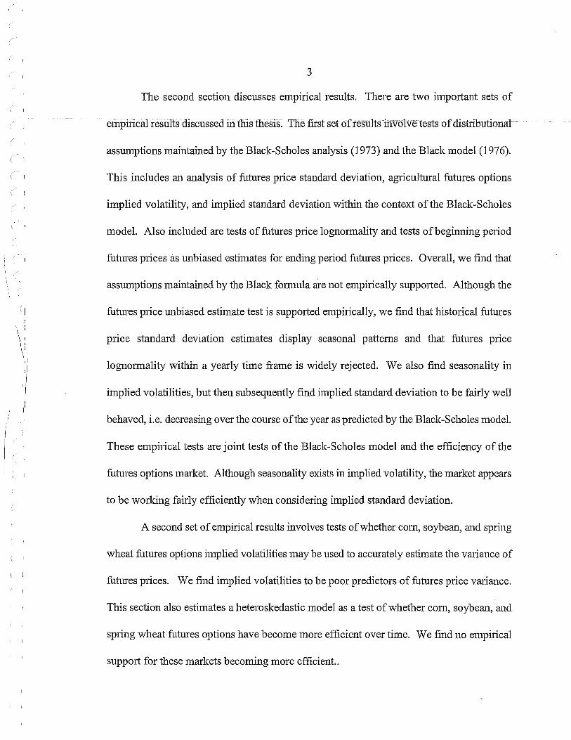
The second section discusses empirical results. There are two important sets of

empilical results discussed in this thesis. The first set of results involve tests of distributional

I I assumptions maintained by the Black-Scholes analysis (1973) and the Black model (1976).

This includes an analysis of futures plice standard deviation, agricultural futures options

implied volatility, and implied standard deviation within the context of the Black-Scholes

model. Also included are tests of futures price lognonnality and tests of beginning period

futmes p1ices as tmbiased estimates for ending period futures prices. Overall, we find that

assmnptions maintained by the Black fonnula are not empirically supported. Although the

I futures price unbiased estimate test is supported empirically, we find that historical futmes

price standard deviation estimates display seasonal pattems and that futures plice

lognormality within a yearly time frame is widely rejected. We also find seasonality in

implied volatilities, but then subsequently find implied standard deviation to be fairly well

behaved, i.e. decreasing over the course ofthe year as predicted by the Black-Scholes model.

These empirical tests are joint tests of the Black-Scholes model and the efficiency of the

futures options market. Although seasonality exists in implied volatility, the market appears

to be working fairly efficiently when considering implied standard deviation.

A second set of empirical results involves tests of whether com, soybean, and spring

\ I wheat futures options implied volatilities may be used to accmately estimate the variance of

I I

futures prices. We find implied volatilities to be poor predictors of futm·es price vmiance.

Tins section also estimates a heteroskedastic model as a test of whether com, soybean, m1d

spling wheat futmes options have become more efficient over time. We find no empirical

support for these mm·kets becoming more efficient..

I '

! '

I I

( i

I '

4

The second section summarizes empirical results and discusses implications for

fhture research. The empirical results found in this thesis are important when discussing ·

future research because they provide a direction which future research should take with

respect to the potential for recovering probabili~tic information from agricultural futures

options.

Several important points are made with respect to future research. First, this thesis

provides evidence that the Black-Scholes distributional assumptions may be inaccurate and

suggests the need to use more flexible distributions as an altemative to the commonly used

lognonnal. Second, option pricing models need to directly incorporate seasonality in futures

price change standard deviation. Such models may then be compm·ed with other, more

general models which do not incorporate seasonality.

5

LITERATURE REVIEW AND MODEL LAYOUT

An Overview ofFutures and Options Markets

A derivative security may be defined as a secmity whose value depends on one or

I ' more tmderlying vmiables. Derivative secmities have become impmiant financial

instruments in recent years, and many different types of derivative secmities are now actively

traded on the mm·ket. Examples of derivative secmities include fmward contracts, futures l ,

contracts, and option contracts. 1

A derivative secmity is also called a contingent claim, since the value or price ofthe

security is contingent on the values of one or more underlying vmiables. Often these

variables are ptices of traded securities, such as with stock options. Derivative securities

( I can essentially be contingent on a host ohmderlying vmiables.

The most basic type of derivative security is called a forward contract. A fmwm·d

contract is simply an agreement between two parties to transact a specified asset at a specific

time in the future at a pre-determined price. A fmward contract is usually between two

financial or other plivate institutions and not traded on an exchange.

There m·e two positions in a forward contract between two parties. One pmiy

assumes a short position and agrees to sell the asset at the specified time at the specified

1For a good introduction and overview of detivative securities, see Hull, John. Options, Futures, and Other Derivative Secmities.

I I

( I

I I

I I

6

price. The other party assumes a long position and agrees to buy the asset at the specified

time at the specified price. The predetermined price at which the asset is transacted is called

the delive1y price, and the time of transaction is generally referred to as the maturity.

In general when first entering into a forward contract, the delivery price is chosen

such that it has zero value to both parties at that particular time. Initially, there is no explicit

cost to take a long or short position in a forward contract. The forward contract is settled at

maturity and can have positive or negative realized value to either of the parties. Although

the contract initially has zero value to both sides, its value is contingent upon the market

price of the asset tmder contract and thus may change over time as the asset's market price

changes.

To better understand fmward contracts, it is necessary to understand the potential

payoffs or losses from entering into the contract. Let the cash price (or spot price) at

matmity be Cr and let K be the delivery price. The payoff to the holder of a long position

in the forward contract is Cr- K and the payoff to the holder of a short position is K - G .

This is because the holder of a long position has an obligation to buy the underlying asset at

the delivery price K and thus gains if Cr > K. The holder of the short position similarly

gains if K > Cr.

Afutures contract is a specific type of forward contract. Like a fmward contract, a

:futmes contract is an agreement between two pmiies to trm1sact a specified asset at a specific

time in the futme for a predetermined price. Unlike forward contracts, however, futmes

contracts are traded on an exchm1ge. The exchange is important because it specifies certain

stm1dm·dized features of the contract such as delivery time (which is usually some pe1iod of

I I

~ I

( I

7

time within a particular month), the amount and quality of the asset for one contract, and the

method in which the futures price is quoted. It also guarantees that the contract will be

honored, since the two parties involved may not necessarily lmow each other. For a

commodity futures contract, the exchange also specifies the product quality and place of

delivery. Fmihermore, the exchange assmes that there is a convenient and consistent method

of quoting prices, and it also assmes that a particular day's trading quickly becomes public

infonnation. Two common exchanges are the Chicago Board of Trade (CBOT) and the

Chicago Mercantile of Exchange (CME). Together, all of the exchanges involve a wide

range of assets which underlie futmes contracts. These include, among others, pork bellies,

cattle, sugar, wool, lumber, copper, aluminum, com, soybeans, and a variety of financial

assets such as stock indices, currencies, Treasury bills, and various types of bonds.

As with forward contracts, there are two sides to a futures contract. One side has

agreed to buy the asset at matmity and has thus taken a long position. The other side has

taken a shmi position and has agreed to sell the underlying asset.

Volume and open interest are two tenns cmmnonly used to characterize the "amolmt"

of futures (or other security) trading that has occurred on a pmiicular day. Volume represents

the total number of contracts that have been traded, while the open interest represents the

nmnber of outstm1ding contracts. An open contract is defined as a contract which has neither

been offset or delivered; it is a contract that remains to be acted upon. To clmi.fy tlns

terminology, suppose that A sells to B.2 A has taken a shmi position and B a long position.

2This tenninology is commonly used as a simple way of saying that A has taken a shmi position in a futmes contract with B.

I '

I I

I I

I I

I I

I I

I !

8

There is one open contract, and thus the open interest is one. If C sells to B, then A is still

short one contract, B is now long two contracts, and C is short one contract. There are two

outstanding contracts and so the open interest is two. IfD then sells to A, A is even, C is still

short one, B is still long two, and D is now short one. The open interest is still two.

Although the open interest is two, there has been a much higher volume of trading than two.

As seen in tlris example, it generally takes a large volume to change the open interest by a

slight amount.

Options are another important type of delivative seculity. Options are contingent

seculities that give the holder the plivilege of enteling into a contract if desired. Options are

now traded throughout the world on a wide range of assets including stocks, stock indices,

foreign cuiTencies, debt instruments, commodities, and various fhtures contracts. This thesis

will be concemed with futures options, which are options on futures contracts.

There are two basic types of futures options. A call option gives the holder the right

to purchase a futures contract by a specified date at a predetermined price. A put option

gives the holder the right to sell a futures contract by a specified date at a predetennined

plice. The predetermined price at which the holder may opt to transact is called the exercise

price or the strike price and is typically denoted X. The specified time by winch the holder

may opt to transact is called the expiration date, the exercise date, or simply 1naturity, and

is denoted T. The fhtures price, which is the plice of the asset tmderlying a futures contract,

is denoted F. The futures price may change over the life of the conh·act, and so it is often

useful to consider the relationslrip of the futures plice at matulity, denoted Fy, with the

futures plice at some time prior to maturity, denoted F,.

I ,

I '

I I

I I

I I

I '

I I

9

When the holder of a futures call option exercises, he or she assumes a long position

in a futures contract plus a cash amount equal to the excess of the futures price (F) over the

strike price (X). When the holder of a futures put option exercises, he or she assumes a short

futures position and receives cash equal to the excess of the strike price (X) over the futures

price (F).

Futures options are further classified based on their exercise possibilities. An option

is said to be European if it can only be exercised at matmity. Ifthe holder may exercise the '

option at any time prior to matmity then the option is said to be American.

It is important to understand that a futmes option contract is different fi·om a futures

contract. In a sole futures contract, the two sides (long and shmi) have entered a binding

agreement and, assuming that the contracts haven't been offset beforehand, a transaction

must take place at maturity. A futmes option contract, on the other hand, gives the holder

the choice of whether or not to transact. Thus, an option gives the holder more flexibility

than does a futmes contract. As a result, entering into a :futmes contract costs nothing

outside of transactions costs (brokers' fees, etc.), whereas an investor must pay for the

"privileges" provided by an option.

There are two sides to every futm·es option contract, and thus a total of fom possible

options positions when considering puts and calls. The investor who has sold the option has

taken a sho1i position, while the investor who has pmchased the option has taken a long

position. The four basic option positions are thus:

10

1. Long call position (purchase a call option) 2. Short call position (sell a call option) 3. Long put position (purchase a put option) 4. Short put position (sell a put option)

To better understand options it is important to tmderstand the potential payoffs

associated with these four options positions.3 First, consider a simple futures option

example. Suppose an investor buys a futures call option. The p1ice of the option is $5, the

ctment futures price (F) is $25, and the option stlike price (X) is $20. Suppose the futures

price rises at matmity to $30. The investor will choose to exercise and realize a payoff of

$30- $20- $5 = $5, assuming no transactions costs. Note that this payoff includes the initial

price of the option, $5. Likewise, if the futures price at maturity is less than $20, then the

holder will clearly choose not to exercise. Note that losses may potentially occur even if the

option is exercised. Suppose for instance the maturity futm·es p1ice is $22. Ifthe holder did

not exercise, he or she would incur a loss of$5, the initial price of the option. Ifthe holder

chose to exercise, however, then he or she would only lose $3. Thus, option exercise may

be optimal in order to minimize losses.

In general, the relationship of the underlying asset price and the strike price

detennines the potential payoffs :fi·om exercise. The payoff :fi·om a long position in a futures

call option is:

MAX(FT -X,O)

3This basic option payoff analysis is similar to options on other secmities (i.e. stocks) as well.

( '

( I

I i

( I

I I

I !

I '

11

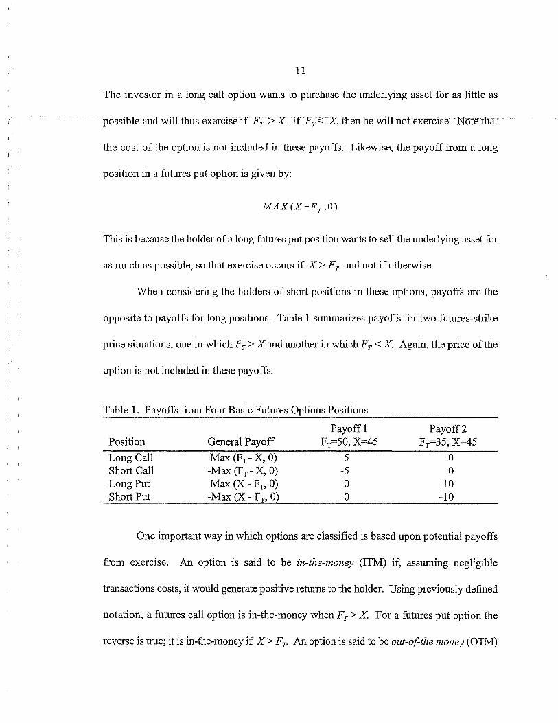
The investor in a long call option wants to purchase the underlying asset for as little as

possible and will thus exercise if Fr >X If Fr< X, thei1 he will not exercise. Note that

the cost of the option is not included in these payoffs. Likewise, the payoff from a long

position in a futures put option is given by:

Tins is because the holder of a long futures put position wants to sell the underlying asset for

as much as possible, so that exercise occurs if X> Fr and not if otherwise.

When considering the holders of short positions in these options, payoffs are the

opposite to payoffs for long positions. Table 1 sUTilmarizes payoffs for two futures-strike

price situations, one in which F T > X and another in whlch F T < X. Again, the price of the

option is not included in these payoffs.

Table 1. Payoffs :limn Four Basic Futures Options Positions

Position

Long Call Short Call Long Put Short Put

General Payoff

Max (FT- X, 0) -Max (FT- X, 0) Max (X - FT, 0) -Max (X- Fn 0)

Payoff1 FT=50, X=45

5 -5 0 0

Payoff2 FT=35, X=45

0 0

10 -10

One important way in winch options are classified is based upon potential payoffs

:li"om exercise. An option is said to be in-the-money (ITM) if, assuming negligible

transactions costs, it would generate positive retun1s to the holder. Using previously defined

notation, a futures call option is in-the-money when Fr >X For a futures put option the

reverse is true; it is in-the-money if X> Fr. An option is said to be out-ofthe money (OTM)

I I

I I

I I

I I

I I

12

if exercise would result in a loss to the holder. Thus, a futures call option is out-of-the

money when X< Fr. Third, an option said to be at-the-money (ATM) ifthe underlying asset

price is equal to the option strike price, so exercise would result in zero return to the holder;

a futures option is thus at-the-money when X= F.

A fuhu·es option (or any option) will only be exercised if it is in-the-money. As will

be discussed later, this method of option classification (ITM, ATM, OTM) will be important

when proposing to use futures options data empirically.

An option may also be characterized by its intrinsic value, which is defined as the

maximum of zero and the value it would have if exercised immediately. A fuh1res call

option's intrinsic value is thus MAX (F,- X, 0). Similarly, the intrinsic value for a fuhu·es put

option is MAX (X- F,, 0). This is directly analogous to the payoffs from futures put and call

options exercise discussed earlier.

Futures and options markets are valuable tools with which to hedge risk. For

instance, a com producer is concemed with harvest time prices throughout the growing year.

He is faced with the probability ofboth increases and decreases in com prices as the growing

season progresses and thus faces risk with respect to the probability of harvest com prices.

As a way to eliminate some of this risk, the producer may take a short position in a com

futures contract to effectively "lock in" his harvest-time price. Altematively, he may

purchase a com fuhrres option which will provide even more flexibility, since the option is

not a binding contract. Keep in mind, however, that flexibility comes at a price. Whereas

it costs nothing to enter into a fuhu·es contract, the hedger must pay for the option.

I I

I I

I I

I I

I I

( I

I I

13

Potential Infonnational Content of Agricultural Futures Options Markets

It has been proposed that the options market for agricultural commodities contains

a wealth of potentially valuable information that could be utilized by those who work in

agriculture. Gardner (1977) proposed that agricultural options may be useful for three

general areas: risk management by individuals, the functioning of tmderlying commodity

markets, and the management of public policy with respect to agricultural production.4

It is impmiant to point out that the tenn "agticultural options" is used fairly generally

here. An option may be written on an agricultural commodity itself (i.e., an option on

physical com), or it may be written on an agricultural cmmnodity futures contract (i.e., an

option on a com futures contract). While Gardner's analysis is concemed with options on

physical commodities, his reasoning may be readily extended to include futmes options,

which is the focus of this thesis.5

The first area of agricultmal interest with respect to the informational content of

futures options involves individual producers, such as the com producer example bliefly

discussed previously. Risk reduction may be done with futures contracts, options contracts,

or a combination thereof, such as with futures options. While the use of futures contracts

4Gardner, Bruce. "Cmmnodity Options for Agticulture." American Jotm1al of Agricultural Economics. December, 1977.

5The reader should be aware of the fact that futures on agricultural commodities have traded for several decades, while futures cmmnodities options are relatively new, having been traded since about 1985. Thus, agticultural futures options were not traded when Gardner published the article in 1977, and options on sole physical cmmnodities were relatively new. Nevetiheless, his analysis is equally applicable to futmes options.

I I

I I

I, I

I I

I I

I I

14

may be effective in hedging risk, options are a more flexible way of dealing with such risks.

Gardner points out that a futures contract fixes the definite price in advance for a hedger.

This is because a futures contract is a binding agreement. An option contract fixes a

potential price over a range of outcomes, yet confronts the producer with prices over a

different range. Futures options are thus a vmy flexible way for producers to deal with risk.

A second agricultural area in which futures options may be useful is public policy and

fann programs. Gardner has proposed that agricultural options prices contain valuable

infmmation regarding the expected vmiability of the tmderlying commodity price. In the

case of a futures option, this would mean that option p1ices contain information not only

about expected futures price variability but also about the commodity spot price vmiability

as well. One area of fm1n policy in which such information may be potentially valuable is

crop instrrm1ce. For instance, when considering rate setting for revenue insurance, estimating

futures price variance is important for statistically detennining actuarially fair premiums.

Since revenue is the quantity of a commodity times the price for which it is sold, estimating

expected price changes is a critical part of revenue insurance analysis.

Heifher (1996) also proposes that cmmnodity fhtures options may contain potentially

useful information in evaluating futures price variability for purposes of crop insurance rate

setting. The tmderlying argument hinges on the fact that futures contracts and futures

options take ctment infonnation into account to provide an "optimal" forecast of fuhrre price

variability. The general notion is that these markets reflect the judgments of traders who

stand to make arbitrage profits if they can forecast better.

I I

I I

I I

( )

I I

15

Heifner's reasoning is thus consistent with Gardner's, and, like Gardner, Heifner

hypothesizes that the options market may be used to estimate expected variability in a way

analagous to the use of futures markets in estimating expected prices.

In summary, futures options may contain potentially useful information that may be

of interest not only to individual producers, but also to those concemed with agricultural

programs and policies such as crop insurance as well as to those wishing to acquire a better

m1derstanding of risks associated with tmderlying commodity markets. One of the primary

purposes of this thesis is to test the hypothesized usefuh1ess of futmes options for com,

soybeans, and spring wheat in predicting futures price variability. Com, soybeans, and

spring wheat are three of the largest agricultmal crops in the world. Furthermore, there is

a large volume of futures options traded on these three crops. Tllis indicates that there is a

sufficiently large amotmt of market information and lends credibility to the hypothesis that

agricultural futmes options markets may potentially be used to accurately assess futmes plice

variability. Specifically, we will look at whether implied volatilities from histolical futures

options prices are accurate predictors of futmes price variance between early (beginning)

peliods and later (ending) peliods within a particular production year. Such a test of futmes

plice variance predictability is fairly general yet has important economic meaning and should

thus be of interest to various areas of agriculture such as those discussed above.

Modeling Futures Plice Movements

A substantial amount of work has been done to model the behavior of asset prices

underlying option contracts. This analysis is specifically concemed with the behavior of

I '

I I

I I

I 1

I '

16

fhtures pdces, which is the underlying variable in a futures option contract. Understanding

the behavior of fuhltes pdces not only helps to tmderstand the nature of the aetna! futures

market itself, but it provides a mechanism with which to model the futures options market

and is necessary when considedng option pdcing theory.

Asset pdces (secudty pdces, futures pdces, etc.) are often assumed to follow a

continuous vmiable, continuous time stochastic model of the fonn: 6

dS

s = 1.1. dt + a dz (1)

S is the asset price, f1 is a growth (or ddft) rate parameter, and adz is a term which adds

random "noise" or vmiability to the growth inS via a scaled Wiener process dz. Technically,

security pdces aren't continuous as such but rather observed in discrete values (such as in

eights) a11d in discrete time intervals (when the exchm1ge is open). h1 practice, such discrete

differences are small, and using continuous variable processes is most useful when modeling

pdce behavior.

The general process given by (1) may be used to model futures pdce movements. For

a futures price, however, the growth rate parameter, fl, is zero. This should be expected,

since it costs nothing to enter into a futures contract agreement. As will be discussed later,

this is also consistent with the use of a "beginning" period futures price as an unbiased

6This model of security pdce motion is known as geometric Brownian motion, which originated in physics to model atomic phenomena. Hull provides a good overview of the model as used in finm1ce to model asset pdce movements.

( I

I I

I I

I I

17

estimate of an "ending" peliod futures plice, so that E( Fr) = F;, where Trepresents an

ending peliod time and t represents some plior time.7

The Lognmmal Distlibution of Futures Pdces

The continuous variable stochastic process used to model futures plices implies

important distlibutional assumptions regarding changes in the futures plice over finite time

intervals. These distributional assumptions are critical in the Black-Scholes analysis, which

will be discussed in detail later.

Black and Scholes (1973, 1976) assume that the futures p1ice follows the general

process given by equation (1 ). Using welllmown results in stochastic calculus, Black (1976)

fiuiher assumes that the futures price is distlibuted lognormally, which means that changes

in the naturallogmithm of the futures price F are normally distlibuted.

To illustrate, suppose that the futures price today is F1 and we are interested in F y; the

futures p1ice at some later timeT. The naturallogmithm ofthe chm1ge in F between t and

T is nonnally distributed a11d is written:

(2)

N (n,m) denotes a nonnal distlibution with mem1 n a11d vmim1ce m. T- tis the time horizon,

Oj is a volatility parmneter eventually lmown as the implied volatility, and e is a growth (or

d1ift) rate parameter.

7T is typically used to denote the contract maturity, but for illustrative purposes may be used to represent any future time.

18

As discussed previously, when specifically consideling futures plices, there is no

expected growth in the futures plice. The expected futures plice at some later time is the

cun·ent futures price, so that E (Fr- FJ = 0, whence Jl = 0 in (1) and 8 0 in (2). Using

mles oflogalithms, equation (2) becomes:

(3)

( I

Equation (3) reflects the fact that there is no expected growth in the futures price. By

considering propetiies ofthe nmmal distlibution, (3) may be futiher rewritten:

(4)

Both (3) and ( 4) are consistent with the notion that E (F -d = F 1, and any change in the futures

I I price over time is the result of random fluctuations, the degree of which is measure by

I !

variance (or standard deviation), which is proportional to the time interval tmder I I

consideration. I I

It is important to point out that the lognonnality of futures prices applies not only to

day to day (infinitesimal) changes but also to longer periods of time. Whether we are

interested in the change in the futures plice in the time peliod of a day or in two months, the

relationship concerning the change inln F1 still has the probability distribution.as given in

equation ( 4).

I I

I I

19

Framework for Empirical Model

There are two important parts of the empirical analysis in this thesis. First, tests of

Black-Scholes option pricing assumptions are perfonned. This may be important for several

reasons. First, the Black-Scholes pricing formulas (including the Black formula) were a

major breakthrough il:i option pricing theory and are probably the most widely used models

to analyze options prices empirically. Second, it is believed that actual option market

participants actively use Black-Scholes models for potential infmmational content.

Furthmmore, tests ofBlack-Scholes assumptions are a tool to guide :fhture research in option

plicing theory.

The second part of the empirical analysis focuses on whether com, soybean, and

spring wheat futmes options contain useful information in predicting futures plice changes.

Specifically, it is hypothesized that volatilities implied in futmes options prices may be good

predictors of changes in futmes price between beginning and ending periods.

These empmcal tests are of interest to those involved in agriculture for a variety of

reasons. As previously discussed, one of the areas in which the informational content of

fhtures options prices may be of potential use is price analysis for crop revenue insurance.

The main problem in statistically determining actuarially fair premiums is finding estimates

of the second and perhaps higher moments of the distribution of possible ending peliod

prices duling a given (beginning) period. An ending peliod futures price on a given day

during the beginning period is considered an unbiased estimate for the mean of possible

futures plices dming the ending period, which is later shown to be empirically supported.

It is a harder task to estimate the vmiance and higher moments of tins distribution of possible

I I

I I

I I

.( I

20

prices. Testing the inf01111ational content of agricultural futures options implied volatility

is thus of direct interest with respect to revenue insurance plice analysis.

When consideling the potential in:f01111ational content of the futures options market,

it is important to tmderstand the basic factors affecting futures options plices. Black and

Scholes (1973) point out that the higher the value of the underlying secmity (a futures plice

in this case), the greater the value of a call option for a given stlike price. 8 As discussed

previously, a futures call option will only be exercised if it is in-the-money, i.e. will generate

positive rettm1s to the holder. Thus, for a futures call, greater chances of option exercise are

present the higher the futtrres plice (F) above the stiike plice (.x). h1 such cases, the value

of the option should be approximately equal to the futures plice (F) minus the plice of a

discount bond that matures at the same time as the option, where the bond has a face value

equal to the option stiike plice (.x). A futures call option will not be exercised if it is out-of-

the money, that is ifF< X If the futures plice (F) is less than the stlilce plice (.x) by a large

enough amount, then it has a value close to 0.9 The value of an option also depends on the

time to maturity as well. Black and Scholes point out that if the matulity is of sufficiently

long duration, then the plice of a bond paying the stlike price (face value) at matmity will

be very low, so that the option value will be close to the futures plice. This makes sense

because if the plice of a futtrres call option exceeded the futtrres plice F, then an arbitrage

8See Myron Scholes and Fischer Black. "The Plicing of Options and Corporate Liabilities." Joumal ofPolitical Economy. 81. May/Jm1e, 1973.

9Black and Scholes (1973) oliginally presented this analysis with respect to options on non-dividend paying stock. These basic plice relationships are applicable to futures options prices, which is of plimary concem in tllis thesis.

I ,

I '

I I

21

profit could be made by taking a long position in the futures contract and selling the futmes

call option. If the expiration time is close, on the otherhand, then the value of a futures call

option will be F- X, if F > X, or 0 if F < X This reflects the fact that the holder of the

futures ca,ll option will exercise ifthe option is in-the-money (F > X) and not ifF < X It is

important to keep in mind that an out-of-the money option does not necessarily have zero

value, because depending on the time horizon and the amotmt by which the option is out-of-

the money, there is always a chance that the option will become in-the-money by expiration

and thus be exercised.

Discussion of these price relationships is important, because it implies upper and

lower botmds which the futures option price must lie between. The upper value of a futures

call option is F, since the option can never be worth more than the futures price. The

minimmn value of the option is 0 or F -X, whichever is larger. Similar bom1ds may be

found for put p1ices.

Option Plicing Models

To test whether options p1ices may be used to predict futures price vatiance, option

pricing models must be considered. A general fonn for option pricing miginally proposed

by Cox at1d Ross (1976) is discussed in Sherrick, et. al. (1996) 10. The only assmnption

required by tllis general option pricing fmmula is that there are no arbitrage opportunities.

10Shenick, Bruce, Philip Garcia, and Viswm1ath Tirupattur. "Recoveling Probabilistic Infonnation from Option Markets: Tests ofDistlibutional Assmnptions." Jotm1al ofFutures Markets. Volume 16. No.5.

I I

I I

i I

( I

I I

I I

I I

I I

I I

I I

22

As Sherrick et. al. point out, "no arbitrage" may be defined as the condition that any two

portfolios with identical distributions of future payOffs have ide11tical current prices, so that

there are no riskless arbitrage opportunities. This is a reasonable assumption, since any

riskless profits resulting from market distortions should be quickly dissipated.

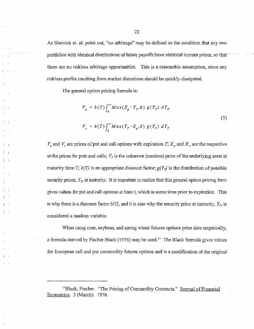
The general option pricing formula is:

(5)

VP and Vc are prices of put and call options with expiration T; XP and X care the respective

strike prices for puts and calls; Yr is the unlmown (random) plice of the underlying asset at

maturity time T; b(T) is an appropriate discmmt factor; g(Y rJ is the distribution of possible

secmity plices, Yr, at matmity. It is important to realize that tllis general option plicing fonn

gives values for put and call options at time t, wllich is some time prior to expiration. Tllis

is why there is a discount factor b(T), and it is also why the security price at maturity, Yr, is

considered a random valiable.

When using com, soybean, and spring wheat futures options plice data empirically,

a fonnula delived by Fischer Black (1976) may be used. 11 The Black fonnula gives values

for European call and put commodity futures options and is a modification of the miginal

11Black, Fischer. "The Plicing of Commodity Contracts." Joumal ofFinancial Economics. 3 (March). 1976.

, I

23

Black-Scholes pricing fmmulas for European put and call options on non-dividend paying

stock.

Several key assumptions underlie the Black formula. As with the original Black-

Scholes analysis, Black assumes that the fhtures price F follows the general stochastic

process given in (1 ), so that :fi:actional changes in the futures price over any finite interval are

lognonnally distributed with lmown, constant variance rate d. Lognmmality is probably the

most common asset price distributional assumption used empirically because it has several

desirable properties. First, lognormality is intuitively simple and mathematically easy to use.

Second, the lognonnal distribution is bounded below by zero, so negative prices are mled

out. Fmihmmore, equal percentage changes either way (for example doubling and halving)

are equally likely tmder lognormality. Tllis is equivalent to assmning that the futures price

follows a random walk process.

Although there are several advantages to using the lognormal distribution as a model

for futures (or other security) price movements over time, Campbell et. al. point out that the

lognonnal may not be entirely consistent with hlstorical secmity price movements. They

suggest that lustorical security price behavior often shows evidence of skewness and excess

kurtosis, neither ofwhlch are accounted for in the lognonnal distribution. 12

The other Black-Scholes assumptions include that there are no transactions costs or

taxes, no risldess arbitrage opportunities, that the risk free interest rate r is constant, and that

12The nmmal distribution has skewness= 0 and kurtosis= 3. Excess kurtosis is defined as the sample kmiosis minus 3.

I '

I '

I '

I ,

I I

I ,

24

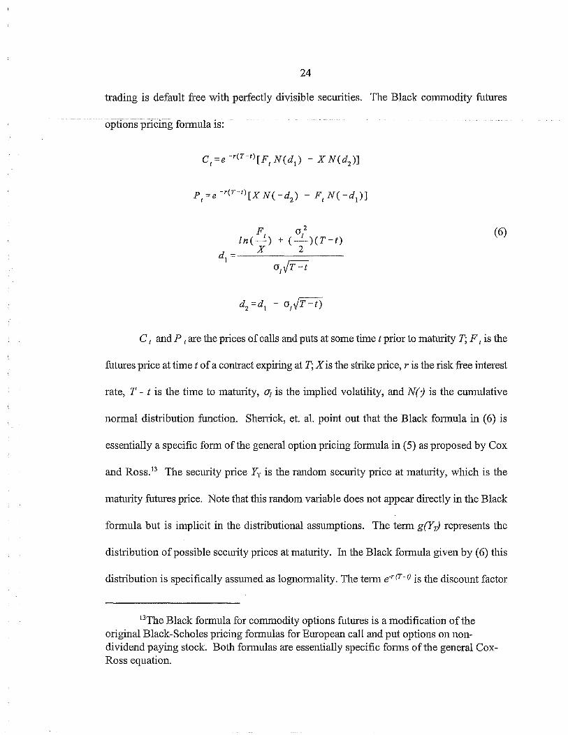
trading is default fi·ee with perfectly divisible securities. The Black commodity futures

options pricing fonnula is:

F 1 a/ ln(-) + (-)(T-t)

X 2 dl=-----------------

aiJr -t

(6)

C 1 and P 1 are the prices of calls and puts at some time t prior to maturity T; F 1 is the

futures price at time t of a contract expiring at T; X is the strike price, r is the risk free interest

rate, T - t is the time to maturity, Oj is the implied volatility, and N( j is the cumulative

normal distribution function. Sheni.ck, et. al. point out that the Black formula in (6) is

essentially a specific fonn ofthe general option pricing fonnula in (5) as proposed by Cox

and Ross. 13 The security price YT is the random security price at maturity, which is the

maturity futures p1i.ce. Note that this random variable does not appear directly in the Black

fonnula but is implicit in the distributional assumptions. The te1m g(Y JJ represents the

distribution of possible security prices at maturity. In the Black formula given by (6) this

distli.bution is specifically assumed as lognormality. The te1m e·r(T-tJ is the discotmt factor

13The Black fonnula for commodity options futures is a modification of the odginal Black-Scholes pli.cing formulas for European call and put options on non­dividend paying stock. Both fonnulas are essentially specific fonns of the general Cox­Ross equation.

I I

25

denoted b(T) in the general formula. The Black formula is essentially an application of

integral calculus to the general option pricing formula given in (5).

The Black-Scholes Parameters

To better tmderstand the Black-Scholes analysis (1973) and the subsequent Black

fonnula (1976), it is necessary to consider the variables which affect futures options prices,

looking qualitatively at how changes in a single variable affect the option price, holding all

others constant. Upper and lower bounds for futures options prices were discussed before

in more general tenns.

The first and probably most important variable affecting the price of a futures option

is the futures price F. 14 For both European and American call options with a given strike

price X, option value increases as the futures price increases. Tins is because the hlgher the

futmes price, ceteris paribus, the greater the chance that the option will be in-the-money and

thus exercised; hence, the more valuable the option. For both European and American put

options, the reverse is true, so that the value of the option declines as the futmes price

mcreases.

The second important variable is the option strike price X. Using similar arguments

as before, the value of futures call options will decrease as the shike ptice increases, since

the holder wants to purchase the underlying futures contract for as little as possible. For

14Similar argmnents could be made for stock options as well. In our case we are primatily concerned with futures options.

I ,.

I '

I I

I I

26

puts, futures options value increases as the strike price increases, since the holder wants to

sell for as much as possible.

Next consider the time to expiration. Here the distinction between European and

American options is important. For American options, it is generally argued that option

holders have more opportunities the longer the time to maturity. Tllis is due to the fact that

they have more exercise opportunities available to them, since American options may be

exercised at any time prior to maturity. Thus, the longer the time to maturity the more

valuable the option, ceteris paribus.

The holders of European options do not have the same exercise possibilities available

to them as do their American counterparts. Thus, it is generally considered ambiguous as

to the changes in the value of the option when the time to maturity increases.

The Black fonnula gives analytic formulas for the value of European fhtures options.

In practice, however, agricultural futures options are American, so that the problem of early

exercise needs to be considered. Black (1976) showed that a futures price is mathematically

analogous to a security which pays a continuous dividend at a rate equal to the risk free

interest rater. Merton (1973) showed mathematically that for the case of a stock option, in

which the stock pays discrete dividends, it is unlikely that early exercise will occur tmtil

possibly just prior to the final dividend payment. It follows that, for a stock wlllch pays a

continuous dividend yield, early exercise will never be optimal. Since a futures option in the

Black model is analogous to a security wlllch pays a continuous dividend yield at rate r, we

conclude that early exercise of agricultural futures option is never optimal. From now on,

( I

I I

I I

I, I

27

fhtmes option will be essentially treated as European, and the distinction between American

and European options will not be important.

The next parameter to consider is the risk free interest rate r. An increase in the risk

fi·ee interest rate will decrease the present value of any future cash flows. Also, the higher

the interest rate the higher the opportunity cost ofbuying futmes options. If the risk fi·ee

interest rate was sufficiently high, the investor would simply invest at this rate, since he

could never do better in the futmes options market. h1 the case of a stock option, an increase

in the interest rate will also have the effect of increasing the expected growth rate of the stock

price. For a futmes option, however, this is not the case. The expected growth rate in a

futures price is zero, which is consistent with using the cmrent futmes price as an tmbiased

estimate of the futures price at some later time. As a result it can be argued that an increase

in the interest rate will decrease the values of both put and call futures options.

The parameter of primary interest in this analysis is the implied volatility, Oj. Under

the stochastic process and distributional assmnptions regarding the underlying futures price

maintained by the Black formula, implied volatility is the constant parameter in (1) such that,

when multiplied by the square root of the time horizon, T- t, gives the market's forecast of

the standard deviation of the change in the natural logarithm of the futures price as seen in

(3).

The implied volatility is thus an "infonnational" parameter because it presmnably

incorporates all relevant market information regarding futme price vmiance as "embedded"

in the price of the option. In accordance with this, Mayhew (1995) defines implied volatility

as the market's assessment of the tmderlying asset's volatility (in our case the volatility of

I '

I '

( '

I I

28

the futures price) as reflected in the option price. For both put and call futures options, the

option price and implied volatility should be positively correlated, so that the higher the level

of implied volatility the higher the price ofthe option.

As discussed earlier, agricultural futures options prices are hypothesized as having

valuable infonnation regarding expected futures price vmiability. When proposing to test

tllis hypothesized infmmational content empirically, several impmiant qualifications must

be made conceming implied volatilities with respect to Black-Scholes assumptions.

Recall that the Black-Scholes analysis assumes that the implied volatility parmneter

is constm1t. Mayhew points out that even ifthe tmderlying asset's volatility is allowed to be

stochastic, then implied volatility may be interpreted as the market's assessment of the

average volatility over the remaining life of the option, and thus should still have potentially

valuable information as to the variability of futures prices expected by the market.

hnplied volatility should properly be considered an "index" or order statistic which

gives the market's best forecast as to the predicted variance of the futures price. This

interpretation of implied volatility is important because, as we will empirically show later,

many ofthe distributional assumptions maintained by the Black formula are rejected. This

may lead one to question the validity of implied volatility as m1 efficient assessment of future

volatility. Tins problem may be reconciled if implied volatility is interpreted as an order

statistic whlch is directly related to the market's assessment of future volatility. Thus,

despite the fact that Black-Scholes assumptions may not be suppmied empilically, it is still

a reasonable hypothesis that implied volatilities may be potentially useful in predicting

subsequent realized futures price variance.

I I

I I

I I

I I

I I

I I

I I

29

An important point emerges from tlris discussion. If the Black-Scholes world was

perfect, then implied volatilities from options differing only by strike price should be

constant, not only across strike prices for a particular trading day but also across the life of

the option contract. Mayhew points out that often times empirically, however, implied

volatilities are found to vary systematically across strike prices and across time, which

Mayhew refers to as the "implied volatility smiles." As we will show later, there is a

systematic seasonal pattern in com, soybean, and spring wheat implied volatilities across

months witlrin a particular year.

Although such seasonal patterns may at first glance be interpreted as strong signs that

the Black-Scholes analysis is incorrect, it is inappropriate to make tills conclusion without

ftuiher considering the market itself. Mayhew points out that the real problem with

"volatility smiles" may be a combination of imperfections in both the market and in the

Black-Scholes model. First, Mayhew points out that market imperfections may prevent

prices fi·om taking their true Black-Scholes values. Second, patterns in implied volatility

across time wlrich are inconsistent with Black-Scholes assumptions may in fact be the result

of a true ftrtures price process wlrich differs from the assumed lognmmal diffusion process.

Mayhew also points out that such phenomenon may be the result of actual option market

participants who strongly rely on Black-Scholes implied volatility quotes when making

trading decisions. It is thus important to realize that tests involving implied volatility are

tests of the market and the Black-Scholes model jointly.

30

Seasonality ofFutures Price Volatility

It has been shown in previous literature that agricultural commodity fhtures price

volatility, which may be generally defined as the variance of futures price changes per time

or the vmiance per time of futures prices themselves, often displays seasonal pattems. It is

typically low in the em·ly pmi ofthe year, such as at or just plior to crop plm1ting, lises m1d

peaks during summer months, and eventually falls as contract matu:tity approaches. Kenyon, ( I

Kling, et. al. (1987) found seasonality in Mm·ch com, March soybeans, and July wheat.

Anderson (1985) tested a null hypothesis of seasonality against a11 altemative of no

seasonality and found strong evidence in support of seasonality for com, wheat, and

soybeans. Anderson concludes that seasonality is an impmiant determinant in futures price

I ' volatility over time. Hennessy and Wahl (1996) summarize anumberoftheories proposed

in previous literature with regard to the causes of such seasonal pattems. 15 Although

I I

hypotheses about seasonality in futu:t·es price volatility are different in many aspects, there

seems to be a consensus that one of the biggest factors affecting futures plice volatility is a

basic pattem ofinfonnation flows. In an early part of the year such as February or Mm·ch,

little is lmown about the expected crop. After the crop is planted and emerges (late Ap1il,

May, or early Jtme) information becomes increasingly available to producers as to expected

crop yields at hm-vest. It is generally m·gued that such infonnation flows lead to resolution

oftmcertainty, which in tu:tn results in an increase in monthly futures price change stm1dard

15Hennessy, David and Thomas Wahl. "The Effects ofFutures Plice Volatility." Americm1 Joumal of Agricultural Economics. 78 (August 1996). 591-603.

I I

I I

I I

i I

31

deviation. Furthermore, there is in general a greater probability that factors occurring during

summer months such as adverse weather may severely hinder growing conditions. To reduce

this potential risk, producers may purchase commodity futures or futures options contracts,

thereby increasing the demand for futures contracts; such infmmation "shocks" will likely

lead to an increase in the standard deviation of futures price changes in these localized

"shock" times.

Hennessy and Wahl (1996) hypothesize that inflexibilities in production and demand

may result in seasonal futures price volatility. In general tenus, their hypothesis rests on the

notion that a decision made on the supply side will make future supply responses more

inelastic. Similarly, decisions made on the demand side will tend to make demand responses

more inelastic.

As the growing season progresses and the actual planted crop begins to grow,

production decisions become more costly, primarily because there is less flexibility in

decision making due to the fact that there are fewer production options available. The supply

cmve thus becomes more inelastic as the season progresses. As harvest approaches, there

is little if any flexibility in production. It is virtUally impossible to produce more output,

given the limited amotmt of time and the lack of feasible production choices. Supply is

nearly fixed at this point.

He1messy and Wahl point out that this "inflexibility" hypothesis is not necessarily

inconsistent with other hypotheses such as the generally accepted "information flows"

hypothesis. h1 fact, it is reasonable to expect information flows and production inflexibilities

to be very closely related.

32

Seasonality in futures price volatility is important when considering the Black­

Scholes analysis, especially when looking at implied volatilities. Since seasonality in futures

p1ice volatility is a fairly well established phenomenon, it will be interesting to test whether

implied volatilities display such seasonal patterns. If the futures options market was efficient

and the Black-Scholes assumptions were accurate, implied volatility should be constant over

the course of a year.

A Method for Testing the Informational Content of Implied Volatility

It is hypothesized that futures options on agricultural commodities contain

information that could be useful in predicting the variance of respective commodity futures

prices. Although there have been a number of previous studies which have tested the

potential informational content of stock options, there has been only limited effort dealing

with agricultural futures options. Beckers (1981), Chiras and Manaster (1977) and Canina

and Figlewski (1993) have investigated the informational content of stock option implied

volatility. The general conclusion is that stock option implied volatilities have not been

found to be good predictors of subsequent realized stock option price variability.

As discussed earlier, the ability of implied volatilities to forecast futures price

variance is of interest to those in agriculture. For example, the problem with respect to crop

insurance is estimating the variance and higher moments of the distribution of ending period

futures prices during the beginning period. The price of a futures contract with ending period

expiration is shown an unbiased estimate for the ending period futures price. As Heifuer

(1996) points out, the futures market is the best source of information available during the

33

beginning period about expected cash (spot) prices during the ending period, since the

market reflects the judgment of informed traders and arbitragers who will profit if they can

forecast better. Thus, it is highly unlikely that there is a better prediction of prices than the

market's. 16

To understand why the beginning period futures price is an unbiased estimate for the

future cash price, it is necessary to understand the relationship between the futures price and

the cash price. Denote F1 the futures price at some time t during the growing season prior

to contract maturity and E(C1 ) the expected maturity cash price at this prior time t. It is

reasonable to expect that the futures price should, on average, be equal to the expected cash

price, so F 1 = E(G). If this relationship did not hold, then arbitrage profits would be

possible. For instance, if F 1 < E(G ), then traders could hold long positions in futures

contracts and anticipate selling at the expected cash price, thereby making positive profits.

IfF,> E(CJJ, a trader should, over a sufficiently long period of time make positive profits

by holding short positions in futures contracts. In equilibrium, we thus expect F1 = E(CJJ,

so that on average the futures price is equal to the expected spot price at maturity. 17

An important result of this discussion is that as the expiration of the contract draws

near, the futures price should converge to the spot price. Thus F1 -- Cr as t -- T, so that

16 Richard Heifuer, "Price Analysis for Determining Revenue Insurance Indemnities and Premiums," Report to the Office of Risk Management, Economic Research Service, USDA.

17See Hull for a more thorough discussion of the relationship between the spot price and futures price of a security.

34

F = C at T. If the futures price were above the cash price, the commodity could be

purchased in the market at the cash price and sold at the futures price. If the cash price were

above the futures price, similar profits would result. Arbitrage between the cash and futures

marl<Zet will assure that the futures price will be equal to the cash (spot) price at contract

maturity. 18

At time T, contract expiration, the distribution of possible cash prices is the same as

the distribution of possible futures prices because of arbitrage arguments discussed above.

One can thus use the futures price at some earlier time t as an expectation for both the futures

price and the cash price at maturity T. At T, cash prices and futures prices may be used

interchangeably, a result that might be of particular relevance for crop insurance rate setting

considerations.

When using futures prices to forecast ending period prices, it is necessary to establish

the appropriate beginning and ending periods for a given commodity, which may vary :fi·om

crop to crop due to production and futures option trading considerations. For com, soybeans,

and spring wheat February is used as the beginning period. Ending periods for these crops

are, respectively, December, November, and September. During a particular beginning

period, futures prices for contracts expiring in these ending periods are used as unbiased

estimates for the ending period futures price.

In this model, a monthly average of beginning period futures prices is used for the

beginning price and is denoted BP. The futures price on the expiration ofthe contract is used

18This discussion is in Hieronymus, The Economics of Futures Trading."

35

as an ending period price and is denoted EP. From these futures prices, a forecast error is

calculated which is defined as the absolute value of the natural logarithm ofthe ratio of the

two prices, denoted lln(ep/bp)i. It is essentially this change which we would like to predict,

since the larger the variance of the beginning period price distribution the larger this absolute

price change.

The parameter of primary interest is ab which is the well known implied volatility

given in equation (6), the Black valuation formula for commodity futures options. Given the

option price (P cor Pp), the strike price (X), the risk free rate of interest (r), and the time to

maturity (T-t), all of which are easily observed, the correct value of implied volatility under

the assumption of lognormality is the one that equates the theoretical option price and the

price observed in the market.

It is not analytically possible to solve equation ( 6) for the implied volatility in closed

fmm as a function of the other parameters. Numerical techniques will be used to search for

the correct value of volatility, which will be discussed in more detail later.

It is again important to distinguish between implied volatility and historical futures

price volatility, both of which have potential uses for predicting future variability. Historical

futures price volatility is an actual variance estimate from historical data. It is an ex-post

measure only, looking back in time at the actual observable behavior of futures prices.

Implied volatility, on the other hand, is a very different measure of variability. Implied

volatility is the constant of proportionality such that when multiplied by the square root of

the time horizon gives the market's best guess for the standard deviation of the futures price

at maturity. As discussed previously, Mayhew defines implied volatility as the market's

36

assessment of the underlying futures price volatility as reflected in the option price19• The

higher the implied volatility, ceteris paribus, the higher the expected futures price variance.

Implied volatility is an order statistic which gives the market's perceived level of future

volatility, which is "embedded" in the price of the option. The higher the perceived level of

variability, the higher the implied volatility and the higher the price of the option. This is

because the higher the level of implied volatility the greater the market's assessment of

future variability. As this variability assessment increases, the more appealing the options

market becomes as a way to reduce future risk, and the more risk writers of options take on

as a result. Prices of options thus increase.

It will be shown empirically that implied volatilities calculated from futures option

premia have a seasonal pattern with peaks in mid-year as information about planted crops

becomes available. Mayhew points out that even if the underlying asset's volatility is

stochastic over time, implied volatility may be interpreted as the market's assessment of the

average volatility over the remaining life of the option.

When proposing to use implied volatilities empirically, several issues must be

addressed. On a given trading day there is a futures price F1 for a particular commodity and

options with several strike prices (Xb A;, ... , A;; ) traded on the same futures contract.

Furthermore, both put and call options are traded. The relationship of the futures price and

strike price is important when considering option theory. As defined earlier, an option is said

to be in-the-money if, assuming negligible transaction costs, it would generate positive

19Stewart Mayhew. "Implied Volatility." Financial Analysts Journal. July­August 1995.

37

returns to the holder if exercised immediately. Thus, a futures call option is in-the-money

if (F- x;) > 0, i.e. the futures price exceeds the strike price. For a put option, the reverse

is true, so that a put is in-the-money if~- F)> 0. An option is said to be out-of-the money

if there would be negative returns upon exercise. An option is at-the-money if the strike

price exactly equals the futures price, so there would be zero return to the holder.

An important issue when considering implied volatility is which strike price to use.

Under Black-Scholes assumptions, options on a particular futures contract differing only by

strike price should have the same implied volatility and should thus be equally useful in

predicting future price variability. Often times empirically, however, different implied

volatilities are obtained from different strike prices on the same contract, a phenomenon

Mayhew (1995) calls the "implied volatility smile." Such a phenomenon raises questions

as to which strike price volatilities to estimate. Mayhew discusses various weighting

schemes to use with implied volatilities obtained from different strike prices. Although

several different weighting schemes have been proposed, the general consensus is that using

options near-the-money seems to work best when testing the potential predictive power of

implied volatilities. Furthermore, trading tends to be most active at options that are near-the-

money. In general these options will likely have higher volumes of trade and thus contain

more information than options that are further in or out of the money. In this paper, options

near-the-money are used: in this paper, near-the-money options are defined as those that are

at-the-money or closest in-the-money.20

20The term near-the-money used in this thesis may not necessarily be defined as in previous literature. There is no standard definition for the term.

38

Another issue is whether to use puts or calls in calculating implied volatility. In

theory, the Black formula predicts that a put option and a call option on the same contract

should yield the same implied volatility. In this study, both puts and calls are used, and

implied volatilities from each group are tested separately as potential predictors for futures

price variance. By doing this we are essentially testing the efficiency of the put and call

market in relation to one another. If puts and calls were not operating "in line" with respect

to one another, then arbitrage opportunities might result. Thus, we expect that implied

volatilities from puts should be highly correlated with implied volatilities from calls, and that

using puts and calls should lead to similar results when considering the information

contained in options prices regarding future price variability.

Fortune (1995) points out that if this were not the case, then one side (puts or calls)

would be overpriced relative to the other. For instance, if implied volatilities from puts

tended to be higher than those from calls, then puts might be "overpriced" relative to calls.

Ifthe reverse was true, then calls might be "overpriced" relative to puts. Fortune continues

to su'ggest that if this was the case, then arbitragers could earn potential profits by purchasing

underpriced options and selling overpriced ones. In short, arbitragers would force puts and

calls back into equilibrium.21

When looking at whether implied volatilities are useful in predicting futures price

variance, alternate beginning periods are used. These beginning periods are moved up from

21Fortune's article discusses and tests the Black-Scholes model with European S&:P 500 stock options. Although he doesn't discuss futures options or the Black formula, the same arbitrage arguments may be used for these types of contracts as well.

39

February until one month prior to the month of contract expiration. Thus, the final beginning

periods for com, soybeans, and spring wheat are, respectively, November, October and

August.

There are several reasons for considering altemate beginning periods. As Heifuer

points out, little is lmown about growing conditions during early months such as February.

As the season progresses, more is lmown about the crop. These information flows may result

in different forecasts of price variance.

Furthermore, by looking at altemate beginning periods, implicit tests of the Black

formula can be made. One important assumption of the Black formula22 is that fractional

changes in the futures price over any interval are lognormally distributed with constant

variance rate d. As seen in equation (3), the variance of ln(Fr!FJ is d (T- t), so that the

standard deviation is av(T- t). It is this volatility parameter, awhich is assumed constant

over time; and a is the parameter which is estimated as the implied volatility from equation

(6). By looking at implied volatilities over successive beginning periods within a particular

year, we will be able to test assumptions maintained by the Black-Scholes model and the

Black formula.

The final day of the contract expiration is used as the ending period price. Futures

contracts normally expire around the twentieth of the month. Options on futures expire just

prior to the futures contract expiration.

22See Fischer Black. "The Pricing of Commodity Contracts." Joumal of Financial Economics. 3 (1976).

40

The previous discussion suggests looking at another measure, the implied standard

deviation.23 As previously discussed, the lognormal assumption of futures prices and the

underlying model of futures price motion implies that ln F r is normally distributed with

standard deviation Oj v(T-t) , which is defined in this paper as the implied standard

deviation. The implied standard deviation may be interpreted as the market's best estimate

for the standard deviation of the distribution of possible futures prices for time T from the

perspective ofthe current (earlier) time t.

Looking at the implied standard deviation is useful for several reasons. First, we will

see if seasonality exists in this implicit measure of variability. Under the Black-Scholes

assumption that the volatility parameter ( a1) is constant, the implied standard deviation

[ a1VrT-t)] should be a monotonic decreasing function across a given year, since T- t IS a

monotonic decreasing function as contract maturity approaches.

Seasonality in the implied standard deviation has important implications for the

Black-Scholes analysis and market performance. First, seasonality in the implied standard

deviation might contradict Black-Scholes assumptions and therefore raise questions as to the

validity of the distributional and motion assumptions of the futures price. Second,

seasonality in the implied standard deviation suggests potential arbitrage opportunities,

which means that the market is not efficiently considering all available information. The

higher the expected variance of the futures price, ceteris paribus the higher the price of the

option. If implied standard deviation did indeed peale, then a potential profit could be made

23This definition only pertains to the analysis in this paper and may not necessarily be the same definition as others have used in previous literature.

41

by purchasing options early in the year when expected variance is relatively low and sold

later when expected variance is high. Such arbitrage possibilities should force implied

volatility and implied standard deviation back into a "no arbitrage" equilibrium.

If there is indeed seasonality in implied standard deviations, then mathematically it

follows that there must also be seasonality in implied volatilities. This is because the implied

standard deviation is the product of the implied volatility ( Oj) and the square root of the time

to maturity ( vT-t), and since the horizon is a monotonic decreasing function over a year, the

implied volatility must unambiguously display seasonality as well, i.e. it must rise and peale

also. To be complete in the analysis it is thus important to look at implied standard deviation

together with implied volatility when considering seasonality, market efficiency and

arbitrage, and the usefulness of the Black formula.

Description of the Data

The data used to find implied volatilities is futures options data obtained from the

Chicago Board ofTrade (CBOT). It contains data for futures options on trading days from

1985, when futures options began trading, through 1996. Data used here includes the day

of trade (timet), the strike price traded on that day (X), a put or call indicator, the expiration

month of the contract (T), the option closing price (P1 or C1), and the volume of trade and

open interest in number of contracts.

As previously discussed, on a given day there is a futures price and options with

several strike prices traded on the same futures contract. From the CBOT data, the option

near-the-money is chosen, which was previously defined as the option at-the-money or

42

closest in-the-money. For instance, if the futures price is 264.50 then the near-the-money

call is that with strike price of260, while the strike price for the near-the-money put was 270.

In some cases the appropriate near-the-money contract had a closing price listed yet had zero

volume, which means it was not traded on that particular day.Z4 These observations were

removed from the data used to numerically find implied volatility. These occurances

typically happen early in the year when trading is fairly thin, such as in February or March.

For com and soybean puts and calls, such zero-volume exclusions are a limited problem, as

on average there are over half of the 23 possible maximum observations. Trading picks up

by March for these crops.

Spring wheat poses the biggest problem with respect to thin trading. For both spring

wheat puts and calls, trading is extremely thin in February, improves slightly in March, and

then picks up to normal levels in April and May.

It should be pointed out that trading generally increases over time. When the futures

options market was new in 1985, it is not too surprising that trading was thin in early

months. By 1996, however, there tended to be more volume traded.

Sample sizes for the monthly com, soybean, and spring wheat futures options data

used to find implied volatilities are included in the appendix.

Once the appropriate futures options data has been obtained, the Black formula may

be used to find implied volatilities. The interest rate p on U.S. Treasury bills adjusted for

24These occurances were typically denoted with an 'N' in the CBOT data files. Although there were no trades on that particular day, a closing price was still listed if the option traded on a previous day.

43

the rate of inflation I is used as the risk free rate of interest, so that r= p - I. The gdp deflator

(chain-type price index) is used to deflate F and X and to calculate inflation rates with which

to adjust the nominal U.S. T -bill rate.25 The time to maturity is based on the number of

calendar days from the day of trade of the option until around the twentieth of the expiration

month, which is used as the expiration ofboth the option and the futures contract26 • When

used in the Black formula, the time to maturity is divided by 365 and expressed as a fraction

of a year.

As discussed earlier, the Black formula gives the price of a call or put option as a

function of several parameters, all of which are observable except the implied volatility. It

is not possible to invert the formula to find volatility as a function of the other parameters.

Therefore an iterative search procedure is used. The search finds the value of implied

volatility such that when plugged into the Black formula, the correct option price (the one

observed in the market) is obtained.

There are different search procedures that may by used to find the implied volatility.

In this study, Fortran was used to try different values ofimplied volatility between 0 and 1

with·a grid search width of .0001. The search was done over the sample of options prices in

a pamcular month. For each value of implied volatility in the Fortran grid search interval,

25Specifically, inflation rates for each year were obtained by subtracting the ratio of the gdp deflator from the subsequent year to the gdp deflator of the current year from one. To obtain the necessary inflation adjustments, averages were used. For example, for 1987, the average of the 1987 and 1986 numbers described above was taken and used for 1987 inflation adjustment.

26The gdp deflator and the interest rate on six month treasury bills (used here as the risk free interest rate) are obtained from Economic Report of the President for 1996.

44

there is a corresponding sum of squared errors for the set of options prices over the entire

month. The program is designed to pick the level of implied volatility that minimizes this

sum of squared errors.27 It should be noted that implied volatility is positive and bounded

below by zero in the limit since the Black formula call and put prices are not defined for zero

volatility.

There are advantages to using the "brute-force" technique in finding implied

volatilities. Such a technique is simple to program and may be executed fairly quicldy.

Furthermore, the search procedure does not rely on curvature properties of the sum of

squared errors :fi.mction, which may adversely affect search algorithms based on numeric

derivatives. In the case in which the sum of squared errors function has more than one

critical point, this numerical technique increases the likelihood that a unique minimum will

be found.

27This search technique has been called the "shotgun" method or the ''brute-force" method.

45

EMPIRlCAL RESULTS

Historical Futures Price Standard Deviation

The most important assumption underlying the Black-Scholes analysis (1973) and

maintained by Black (1976) is that the futures price F follows a lognormal diffusion process

of the general form

dF

F = !l dt + a dz (la)

where Jl is a constant growth rate parameter and adz is a random noise Wiener process in

which the volatility parameter a is assumed constant. The reader should be aware that the

general form (la) is given without loss of generality, as !l = 0 for a futures price. As a result

of this process it is further assumed that fractional changes in F over a time interval lJ.t are

lognormally distributed with zero mean and variance d lJ.t, or equivalently a standard

deviation of avYiJ.t), which is consistent with equation (3).

To partially test these distributional assumptions, the standard deviation of the natural

logarithm of fractional price changes of the form

is calculated for a particular month, where t represents a trading day and t-1 the previous

trading day within that month. If markets were perfect and the Black-Scholes model was

46

accurate, the standard deviation in these monthly "log-fractional" changes should be constant

across a giVen year.

As previously discussed, it has been shown in previous literature (i.e. Hennessy,

et.al.) that historical futures price volatility often displays seasonal patterns, typically

showing peaks during summer months. It is thus of interest to see if standard deviation in

"log..:fractional" changes over successive months within a year display similar seasonal

"peaks."

Tables 2 through 4 show standard deviations for monthly "log-fractional" changes

for com, soybeans, and spring wheat futures prices over successive months. Com and

soybean futures prices show seasonal patterns. Com has five peaks in June, four in July, and

one "late" peak each in August, September, and October. Soybeans show three peaks in

June, seven in July, and one each in May and August. Overall, June and July appear to be

the "peak" months for com and soybean futures prices.

As seen in table 3, spring wheat futures prices also display seasonality, although the

seas0nal pattern is much less strong than for com and soybeans. Spring wheat peaks are

spread out across successive months. May, July and August have two peaks; the remaining

months each have one peale

Overall, there is strong seasonality for com and soybeans, and peaks for these crops

occur primarily in June or July. Spring wheat shows less strong evidence in seasonality, as

there are pealcs not only in mid-year but also in early and late months as well.

This overall pattern of seasonality in monthly "log-fractional" price changes does not

support assumptions maintained by the Black formula. It is again important to realize,

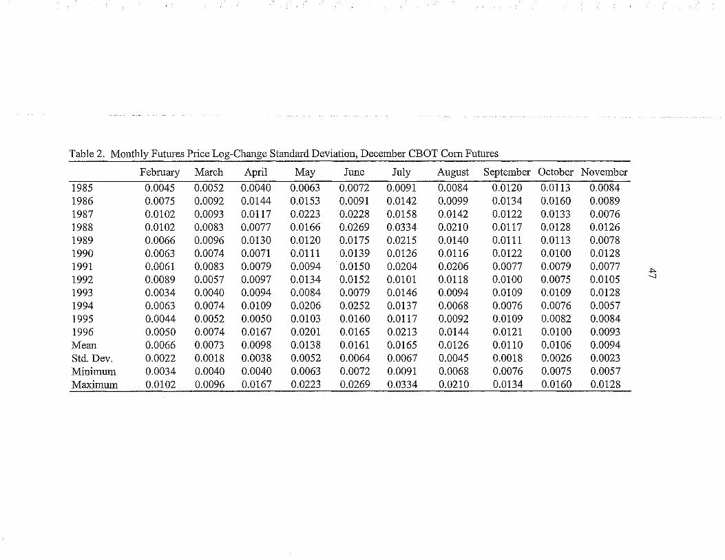
Table 2. Monthly Futures Price Log-Change Standard Deviation, December CBOT Com Futures

February March April May Jlme July August September October November

1985 0.0045 0.0052 0.0040 0.0063 0.0072 0.0091 0.0084 0.0120 0.0113 0.0084 1986 0.0075 0.0092 0.0144 0.0153 0.0091 0.0142 0.0099 0.0134 0.0160 0.0089 1987 0.0102 0.0093 0.0117 0.0223 0.0228 0.0158 0.0142 0.0122 0.0133 0.0076 1988 0.0102 0.0083 0.0077 0.0166 0.0269 0.0334 0.0210 0.0117 0.0128 0.0126 1989 0.0066 0.0096 0.0130 0.0120 0.0175 0.0215 0.0140 0.0111 0.0113 0.0078 1990 0.0063 0.0074 0.0071 0.0111 0.0139 0.0126 0.0116 0.0122 0.0100 0.0128 1991 0.0061 0.0083 0.0079 0.0094 0.0150 0.0204 0.0206 0.0077 0.0079 0.0077 ..j::.

1992 0.0089 0.0057 0.0097 0.0134 0.0152 0.0101 0.0118 0.0100 0.0075 0.0105 ..._..

1993 0.0034 0.0040 0.0094 0.0084 0.0079 0.0146 0.0094 0.0109 0.0109 0.0128 1994 0.0063 0.0074 0.0109 0.0206 0.0252 0.0137 0.0068 0.0076 0.0076 0.0057 1995 0.0044 0.0052 0.0050 0.0103 0.0160 0.0117 0.0092 0.0109 0.0082 0.0084 1996 0.0050 0.0074 0.0167 0.0201 0.0165 0.0213 0.0144 0.0121 0.0100 0.0093 Mean 0.0066 0.0073 0.0098 0.0138 0.0161 0.0165 0.0126 0.0110 0.0106 0.0094 Std. Dev. 0.0022 0.0018 0.0038 0.0052 0.0064 0.0067 0.0045 0.0018 0.0026 0.0023 Minimum 0.0034 0.0040 0.0040 0.0063 0.0072 0.0091 0.0068 0.0076 0.0075 0.0057 Maximum 0.0102 0.0096 0.0167 0.0223 0.0269 0.0334 0.0210 0.0134 0.0160 0.0128

Table 3. Monthly Futures Price Log-Change Standard Deviation, November CBOT Soybeans

Februruy March April May Jm1e July August September October

1985 0.0071 0.0076 0.0073 0.0085 0.0114 0.0165 0.0095 0.0106 0.0081 1986 0.0052 0.0076 0.0122 0.0103 0.0078 0.0141 0.0102 0.0072 0.0098 1987 0.0053 0.0062 0.0104 0.0249 0.0224 0.0198 0.0077 0.0075 0.0111 1988 0.0096 0.0104 0.0117 0.0184 0.0270 0.0350 0.0211 0.0147 0.0138 1989 0.0101 0.0101 0.0106 0.0120 0.0153 0.0222 0.0176 0.0098 0.0083 1990 0.0053 0.0085 0.0083 0.0128 0.0135 0.0129 0.0108 0.0096 0.0104 1991 0.0063 0.0089 0.0086 0.0079 0.0127 0.0214 0.0258 0.0104 0.0133 ,.J:::..

1992 0.0093 0.0073 0.0067 0.0124 0.0137 0.0091 0.0107 0.0085 0.0063 00

1993 0.0049 0.0057 0.0051 0.0059 0.0127 0.0167 0.0141 0.0146 0.0070 1994 0.0051 0.0066 0.0062 0.0226 0.0231 0.0137 0.0070 0.0079 0.0076 1995 0.0042 0.0070 0.0073 0.0137 0.0137 0.0167 0.0087 0.0141 0.0070 1996 0.0063 0.0066 0.0154 0.0101 0.0140 0.0187 0.0105 0.0128 0.0134 Mean 0.0065 0.0077 0.0091 0.0133 0.0156 0.0181 0.0128 0.0107 0.0097 Std. Dev. 0.0020 0.0015 0.0030 0.0058 0.0056 0.0065 0.0058 0.0028 0.0027 Minimum 0.0042 0.0057 0.0051 0.0059 0.0078 0.0091 0.0070 0.0072 0.0063 Maximmn 0.0101 0.0104 0.0154 0.0249 0.0270 0.0350 0.0258 0.0147 0.0138

Table 4. Monthly Futures Price Log-Change Standard Deviation, September CBOT Spring Wheat

February March April May June July August

1987 0.0117 0.0082 0.0127 0.0197 0.0140 0.0122 0.0097 1988 0.0077 0.0092 0.0089 0.0157 0.0361 0.0304 0.0127 1989 0.0079 0.0119 0.0077 0.0081 0.0098 0.0116 0.0063 1990 0.0044 0.0049 0.0083 0.0079 0.0068 0.0093 0.0147 1991 0.0096 0.0122 0.0085 0.0080 0.0136 0.0167 0.0220 1992 0.0185 0.0111 0.0104 0.0150 0.0113 0.0116 0.0115 1993 0.0088 0.0072 0.0074 0.0086 0.0090 0.0172 0.0117 ..j:::..

1994 0.0084 0.0085 0.0123 0.0153 0.0139 0.0106 0.0099 1.0

1995 0.0078 0.0090 0.0111 0.0136 0.0168 0.0201 0.0191 1996 0.0097 0.0121 0.0272 0.0205 0.0192 0.0177 0.0126 Mean 0.0094 0.0094 0.0114 0.0132 0.0151 0.0157 0.0130 Std. Dev. 0.0037 0.0024 0.0059 0.0049 0.0083 0.0063 0.0046 Minimmn 0.0044 0.0049 0.0074 0.0079 0.0068 0.0093 0.0063 Maximum 0.0185 0.0122 0.0272 0.0205 0.0361 0.0304 0.0220

50

however, that such tests are not tests solely ofBlack-Scholes, but rather joint tests of market

efficiency and Black-Scholes together. Seasonality is contradictory not only with respect to

the Black-Scholes analysis, but also because it seems plausible that the market should

prop~rly adjust to such seasonal patterns. Implications of seasonality for both the Black-

Scholes model and the futures options market itself will be discussed further when

considering implied volatility and implied standard deviation.

Futures Price as Unbiased Mean Estimate

As discussed earlier, futures options prices are hypothesized to contain infonnation

which may be used to predict futures price variability, and as such may be of interest to

different areas of agriculture. For example, crop insurance may be interested in whether

futures options contain information which may be used to predict futures price variance with

respect to beginning and ending periods.

When considering the distribution of possible ending period futures prices, the futures

price during a particular beginning period is used as an unbiased estimate for the ending

period price. If not, then arbitrage opportunities would be possible in the cash-futures

market; it is unlikely that there is a better forecast than the futures market's regarding ending

'

period prices.

To test whether beginning period futures prices are indeed unbiased estimates for the

ending period futures price, ending period futures prices are regressed on average futures

prices during beginning periods ranging from February until one month prior to contract

51

expiration. The appropriate ending period price is the final trading day futures price for the

particular commodity futures contract (i.e. December for com, November for soybeans, and

September for spring wheat.)28

The estimated empirical form is:

EP = ex + PCBP)

BP is the average futures price during a particular beginning period, for instance the average

Febmary futures price on the December com contract. EP is the futures price on the final

day ofthe contract expiration month, i.e. December 20 for com. This regression is run for

each beginning period using futures data from 1960 through 1996. It thus includes Febmary

through November on the December com contract, Febmary through October on the

November soybean contract, and Febmary through August on the September spring wheat

contract.

If beginning period futures prices are indeed unbiased mean estimates for ending

period futures prices, then we would expect beta not to differ significantly from one. This

is because on average we expect the beginning period futures price to equal the ending

period price. Put differently, although it is totally reasonable to expect futures prices to

differ occasionally from actual realized ending prices, there should as many above as below,

so that an estimate of p = 1 should still result.

Tables 5 through 7 show "OLS expected futures price" tests for com, soybeans, and

spring wheat for successive beginning periods from 1960 through 1996. Shown is the

28This final day is around the 20th of the contract expiration month.

52

estimated intercept alpha, the estimated slope beta (with standard errors in parentheses), and

at-test of whether beta is significantly different from 1. The appropriate t-statistic is given

by:

/}* is the estimated slope coefficient and SE is the standard error. A high value of this

statistic indicates that beta is significantly different from one.

Table 5. Futures Price Unbiased Estimate Test for Com, OLS Test

Alpha Beta T -test forBeta;e 1

February .2101 .9492 -.4190 (.5259) (.1213)

March .0077 .9992 -.0068 (.5326) (.1234)

April -.0796 1.0199 .1500 (.5713) (.1327)

May -.3861 1.0975 .7558 (.5521) (.1290)

June -.5003 1.1080 .9626 (.4884) (.1122)

July -.2211 1.0350 .5132 (.3024) (.0682)

August .2812 .9157 -2.1022 (.1810) (.0401)

September .1685 .9509 -1.3016 (.1681) (.0377)

October .2438 .9359 -2.0808 (.1376) (.0308)

November .0671 .9824 -.8904 (.0874) (.0198)

Note: Standard Errors in Parentheses Sample size includes 37 years of futures data from 1960-1996

53

Table 6. Futures Price Unbiased Estimate Tests for Soybeans, OLS

Alpha Beta Beta* 1

February -.0560 1.0419 .3923 (1.038) (.1 068)

March -.2819 1.0629 .5803 (1.0550) (.1084)

April -.4572 1.0790 .6524 (1.1770) (.1211)

May -.8842 1.1161 1.1089 (1.026) (.1047)

June .2497 .9756 -.2802 (.8786) (.0870)

July .7119 .9109 -1.6748 (.5530) (.0532)

August 1.7646 .8010 -3.7688 (.5577) (.0528)

September .7853 .9072 -2.3671 (.4075) (.0392)

October 1.0427 .8898 -3.2896 (.3457) (.0335)

Note: Standard errors in parentheses, sample size includes 37 years, 1960-1996

Table 7. Futures Price Unbiased Estimate Tests for Spring Wheat, OLS Test

Alpha Beta Beta* 1

February .9348 .8619 -1.1042 (.7659) (.1251)

March .6141 .9341 -.4985 (.7905) (.1322)

April -.0386 1.0595 .4250 (.8218) (.1400)

May -.6314 1.1739 1.2872 (.7841) (.1351)

Jtme -.4009 1.1213 1.0773 (.6645) (.1126)

July -.2121 1.0832 .9265 (.5368) (.0898)

August -.0824 1.0386 1.5820 (.1510) (.0244)

Note: Standard errors in parentheses, sample size includes 37 years, 1960-1996

54

For soybeans, we find that there are more beginning months for which beta appears

to differ significantly differ from one. There is marginal significance for May and July, and

more significance for August, September, and October. Again, this may result from alpha

estimates that are significantly different from zero.

For spring wheat, February, May, June, and August have betas which are marginally

different from one. The alphas for these months, however aren't significantly different from

zero except for February, which is only marginally different.

Overall, the notion that futures prices early in the year are optimal forecasts for prices

later in the year is fairly well supported. Although there are instances in which the estimated

slope differs significantly from one, it may still be reasonable to conclude that the theory

holds since it could very well be the result of alpha estimates which differ significantly from

zero.

This "futures price unbiased estimate" hypothesis is tested another way, which is

discussed in Judge, et.al: Specifically, when considering the OLS empirical form discussed

earlier in this section, it is hypothesized a=O and ~= 1; as discussed in Judge, et.al., our null

hypothesis is that the coefficients are restricted. We thus test the null (restricted) hypothesis

against the alternative that the coefficients are unrestricted. The appropriate test statistic is:29

SSER - SSEU A = ------ ~ F(J,T-K)

Jaz e

29For a description of this test see Judge, et. al. Introduction to the Theory and Practice ofEconometrics, 1988.

55

SSER and SSF.u are the sums of squared errors, respectively, from the restricted and

unrestricted models, Tis the sample size, J is the number of constraints, K is the number of

parameters in model, and o/ is an estimate for the unrestricted error variance. Specifically,

an estimate for o/ used here is SSEu IT- K. fu our case, J and K are 2, and the sample size

Tis 3 7, which represents the number of years from 1960 through 1996 in which futures data

is taken.

Given a level of significance alpha, the null hypothesis that the coefficients are

restricted is rejected if the sample statistic A.- F(J, T-K,o:) is larger than the critical F-value at

that particular alpha. If the reverse is true, so that the sample statistic A is smaller than the

critical F-value, then we do not reject the null hypothesis and thus conclude that the

estimated coefficients are not significantly different from their hypothesized (restricted)

values.

Table 8 summarizes results of the "restrictions" test for com, soybeans, and spring

wheat for two separate cases. The first case includes the outlier 1973, the year in which

prices made a seemingly discontinuous jump as a result of the grain embargo of 1972. The

second case is with 1973 removed. This is done to see if results improve significantly.

For com, results support the hypothesis that beginning period futures prices are

unbiased estimates for ending period futures prices. fu the case in which 1973 is included,

none of the months are rejected, although October appears to be "worse" than the other

months. fu the no-1973 case, October is rejected, and it appears that removing 1973 did not

result in significant improvement.

Table 8: Futures Price Unbiased Estimate Test for Com, Soybeans, and Spring Wheat: Restrictions Test

Dece1l1ber Com Novefnoer Soybear1s September Spring Wheat

With 1973 Without 1973 With 1973 Without 1973 With 1973 Without 1973

February .0877 .1473 .8045 .3392 .7496 2.6640 March .0007 .2769 .7857 .3007 .5293 .7609 April .0114 .2044 .6789 .2473 .7216 .1529 May .2916 .1897 .9600 .5480 1.7926 .8121 Jtme .5286 .4300 .0409 .0822 1.4012 .3140 July .4401 .8014 1.8546 .1559 1.3620 .5436 August 2.8672 1.2124 7.6579 1.2317 4.0790 2.0454 September 1.0393 2.4564 3.2445 1.2701 *********** *********** October 2.2689. 5.4783 5.4470 5.2703 *********** *********** November .4179 2.1027 ********* *********** *********** ***********

Note: Boldface indicates rejection of hypothesis that begimung futures price is an tmbiased estimate for ending futures price The critical x2 statistic is 5.285 when1973 is included and 5.306 when1973 is removed as an outlier

Vl 0\

57

For soybeans, August and October are rejected when 1973 is included. Results

improved significantly when 1973 is removed; in the no-1973 none of the months are

rejected.

For spring wheat none of the months are rejected, both when 1973 is included and

when1973 is removed as an outlier.

Overall, results based on the "restrictions" tests are extremely favorable for com and

spring wheat. Results appear overall less favorable for soybeans, although throwing out

1973 makes a significant improvement: one month is rejected without 1973 as compared to

three months rejected with 1973.

Futures Price Lognormality

Probably the most important assumption maintained by the Black-Scholes analysis

is that futures price changes are distributed lognormally. It is thus appropriate to test the

hypothesis that futures price changes are lognormally distributed for com, soybeans and

spring wheat. Rejecting lognormality has serious implications for the Black formula.

Lognormality is tested in the following way. Using deflated futures prices, the

natural logarithm of the ratio of a trading day's futures price to the previous trading day's

futures price is calculated within a year. These yearly futures prices range from February

through the appropriate final beginning period (November for com, October for soybeans,

and September for spring wheat). The series of price changes obtained is then regressed

against a constant, 1, using a no-constant model. This technique allows us to look at the

normality of residuals to determine normality of the actual price changes themselves. The

58

appropriate test statistic is the Jarque-Bera statistic, which is distributed X2 with two degrees

of :freedom in this case. Lognormality is rejected if the chi-squared statistic is too large.

Tests oflognormality are critical when evaluating assumptions made by the Black

Fonnula. One reason that lognormality is rejected often may be the result of problems with

skewness and kurtosis. Sherrick, et.al. point out that the lognormal distribution is not

considered to be very flexible because it does not allow for varying degrees of skewness and

kurtosis. As presented in Campbell, et.al., skewness, or the normalized third moment, of a

random variable Ewith mean Jl and variance30 dis:

Skewness is a measure of the degree to which the distribution "leans" to one side or the

other and may be positive or negative. The normal distribution is symmetric and thus has

zero iskewn~ss.

Kurtosis is the normalized fourth moment and, using similar notation, is defined by:

Kurtosis is a measure of how "fat" the tails of the distribution are. Thus, the more

probability mass ("fatter") included in the tails, the higher the kurtosis of the distribution.

The kurtosis of a normal distribution is 3.

30:0o not confuse these generic distributional parameters with those specifically defined and used throughout this thesis.

59

It is suspected that non-zero skewness and excess kurtosis, defined as sample kurtosis

minus three, may be two key problems which result in rejection oflognormality (remember

that when testing for lognormality we are actually testing the normality of the natural log of

the fractional price changes).

Tables 9 through 11 give estimated Jarque-Bera statistics, coefficients of skewness,

and coefficients of excess kurtosis (with t-statistics in parentheses) for corn, soybeans, and

spring wheat data from 1960 through 1996. Overall, lognormality is strongly rejected. For

December corn futures prices, 21 of the possible 37 years from 1960 through 1996 are

rejected. For November soybeans, 25 of the years are rejected, and for September spring

wheat 18 of the years are rejected. When considering all three crops collectively over these

37 years, lognormality is rejected almost sixty percent of the time.

It is worthwhile to examine the coefficients of skewness and excess kurtosis and

compare years in which lognormality is rejected with years in which lognormality is not

rejected. If the distribution of futures prices was truly lognormal, then the coefficients of

skewness and excess kurtosis, hereafter denoted C(s) and C(k), should be close to zero. For

years in which lognormality is not rejected, C(s) and C(k) are usually not significantly

different from zero. For years in which lognormality is rejected, there are fairly high t-values

for C(s) and C(k). Furthermore, by inspection ofthe table it appears that kurtosis is likely

to be the most "significant" problem that results in rejection oflognormality.

Sherrick et. al. have also tested lognormality for soybean futures prices. By looking

at monthly data for 22 different months between March 1988 and March 1991, Sherrick et.

al. reject lognormality about a third ofthe time. Sherrick et. al point out that these results

60

Table 9. Lognorma1ity Tests for December CBOT Com Futures Prices, Jarque-Bera~x2(2)

Jarque-Bera Statistic Coefficient of Skewness Coefficient ofExcess Kurtosis

1960 75.9851 -.0235 2.9449 (-.1445) (9.0948)

1961 1.3495 -.1215 .3291 (-.7459) (1.0142)

1962 433.9476 .7290 6.8923 (4.4533) (21.1485)

1963 1117.0126 .2781 11.2539 (1.7030) (34.6061)

1964 6.4969 .1230 .8453 (.7551) (2.6049)

1965 7.9622 .3358 .6805 (2.0652) (2.1016)

1966 100.9831 -.1298 3.3889 (-.7986) (10.4435)

1967 26.2786 .0395 1.7456 (.2425) (5.3794)

1968 135.9788 1.0148 3.3745 (6.1991) (10.3544)

1969 372.1339 -.4990 6.4672 (-3.0427) (19.8016)

1970 179.4807 .9046 4.1296 (5.5531) (12.7260)

1971 33.5260 .0139 1.9653 (.0855) (6.0695)

1972 160.0029 .3994 4.1934 (2.4518) (12.9227)

1973 5.1144 -.1290 -.6901 (-.7866) (-2.1130)

1974 9.1232 -.0234 -.9895 (-.1429) (-3.0362)

1975 2.9412 .2569 -.2179 (1.5732) (-.6700)

1976 22.3239 .1896 1.5652 (1.1639) (4.8234)

1977 4.3695 -.1860 .6183 (-1.1418) (1.9054)

1978 .8833 -.0659 .3139 (-.4036) (.9653)

Note: Boldface: Lognorma1ity not rejected, ex .005, sample size ;:: 230 per year. T -values for skewness/kurtosis shown in parentheses.

61

Table 9 (cont.)

Jarque-Bera Statistic Coefficient of Skewness Coefficient ofExcess Kurtosis

1979 6.0882 -.2338 .7079 (-1.4317) (2.1768)

1980 1.5135 .1547 .2965 (.9473) (.9117)

1981 .0927 -.0176 -.0682 (-.1082) (-.2106)

1982 24.5629 -.1162 1.6735 (-.7133) (5.1572)

1983 3.8462 .3230 .0055 (1.9865) (.0170)

1984 10.4736 -.1162 1.0846 (-.7146) (3.3496)

1985 21.6373 .5857 1.1191 (3.4822) (3.3416)

1986 44.2118 .5515 2.0532 (3.2711) (6.1162)

1987 14.7366 -.2831 1.2310 (-1.6831) (3.6757)

1988 3.8642 -.0773 .6895 (-.4617) (2.0613)

1989 29.4426 -.0082 1.9078 (-.0489) (5.7103)

1990 8.6004 -.3747 .7003 (-2.2330) (2.0961)

1991 38.1278 .1794 1.0666 (2.1413) (6.3938)

1992 30.4704 -.4997 1.6652 (-2.9568) (4.9486)

1993 58.8582 .7348 2.2334 (4.3686) (6.6689)

1994 138.0692 -.4469 4.0054 (-2.6570) (11.9600)

1995 46.4168 .0103 2.3133 (.0632) (7.1288)

1996 .2226 .0394 -.1110 (.2386) (-.3376)

Note: Boldface: Lognormality not rejected, ex= .005, sample size :::;< 230 per year. T -values for skewness/kurtosis shown in parentheses.

62

Table 10. Lognonnality Tests for November Soybean Futures Prices, Jarque-Bera-x2(zJ

Jarque-Bera Statistic Coefficient of Skewness Coefficient of Excess Kurtosis

1960 62.4081 .0251 2.8141 (.1470) (8.2841)

1961 411.9714 -.8835 6.9545 (-5.1757) (20.4725)

1962 1233.1139 .7987 12.3325 (4.6680) (36.2188)

1963 81.8752 -.0194 3.2276 (-.1134) (.3405)

1964 265.9895 .6253 5.6669 (3.6461) (16.5990)

1965 82.8431 -.0851 3.2335 (-.4985) (9.5187)

1966 42.0171 .1720 2.2940 (1.0053) (6.7372)

1967 294.1186 .8012 5.8508 (4.6936) (17.2234)

1968 69.3496 .1327 2.9765 (.7720) (8.6981)

1969 54.8447 .0653 2.6651 (.3790) (7.7700)

1970 51.7057 .5197 2.3481 (3.0303) (6.8779)

1971 29.7326 -.2810 1.8650 (-1.6462) (5.4901)

1972 18.6633 .1268 1.5308 (.7428) (4.5063)

1973 3.5333 .0292 -.6345 (.1699) (-1.8542)

1974 9.7699 .0142 -1.0793 (.0826) (-3.1540)

1975 1. 7938 .0715 -.4212 (.4169) (-1.2337)

1976 3.5453 -.0580 -.6245 (-.3390) (-1.8341)

1977 .3970 -.0658 .2081 (-.3846) (.6112)

1978 16.9068 -.6331 .7019 (-3.7002) (2.0614)

Note: Boldface: Lognonnality not rejected, a = .005, sample size :::: 200 per year. T -values for skewness/kurtosis shown in parentheses.

63

Table 10 (cont.)

Jarque-Bera Statistic Coefficient of Skewness Coefficient ofExcess Kurtosis

1979 12.7615 -.3488 1.0701 (-2.0434) (3.1501)

1980 .2854 .0554 .1825 (.3230) (.5346)

1981 4.6874 -.0244 .7938 (-.1426) (2.3313)

1982 .9223 .0759 -.2719 (.4436) (-.7985)

1983 .5294 .1255 .0078 (.7352) (.0230)

1984 23.2718 -.4250 1.4889 (-2.4956) (4.3933)

1985 67.0444 .8081 2.5360 (4.5707) (7.2086)

1986 19.6940 .2105 1.5988 (1.1906) (4.5446)

1987 61.8960 -.1388 2.8976 (-.7851) (8.2365)

1988 7.5471 -.3738 .6843 (-2.1202) (1.9501)

1989 10.2196 -.2641 1.0712 ( -1.4938) (3.0449)

1990 1.4641 -.0329 .4701 (-.1861) (1.3363)

1991 82.7556 .1024 3.3550 (.5792) (9.5367)

1992 13.4718 -.4397 1.0434 (-2.4744) (2.9508)

1993 65.3678 -.0834 2.9863 (-.4717) (8.4886)

1994 155.7526 -.4939 4.5006 (-2.7872) (12.7604)

1995 121.0458 .0494 3.9067 (.2894) (11.5004)

1996 7.7789 -.2647 .8525 (-1.5507) (2.5096)

Note: Boldface: Lognormality not rejected, ex= .005, sample size~ 200 per year. T -values for skewness/kurtosis shown in parentheses.

64

Table 11. Lognormality Tests for September Spring Wht. Futures Prices, Jarque-Bera~x2(2l

Jarque-Bera Statistic Coefficient of Skewness Coefficient ofExcess Kurtosis

1960 .5561 .1403 .1113 (.7357) (.2935)

1961 94.4796 -.7750 3.5855 (-4.0386) (9.3984)

1962 19.1245 -.4152 1.5732 (-2.1569) (4.1119)

1963 8.6900 .1518 1.1794 (.7886) (3.0826)

1964 8.8466 -.2874 1.0719 (1.5849) (2.8097)

1965 3.2785 .1634 .6775 (.8542) (1.7815)

1966 30.6383 .2345 2.1905 (1.2258) (5.7599)

1967 17.2079 -.5895 1.1700 (-3.0719) (3.0852)

1968 10.4285 -.5766 .5848 (-2.9860) (1.5237)

1969 39.7601 -.6151 2.2523 (-3.1755) (5.8501)

1970 774.3505 .7070 11.0661 (3.6842) (29.0068)

1971 16.5030 .6377 .9972 (3.3335) (2.6221)

1972 57.0802 .9928 2.2607 (5.1898) (5.9445)

1973 12.1355 -.2371 -1.2714 (-1.2317) (-3.3231)

1974 5.2389 .0493 -.8765/ (.2553) (-2.2837)

1975 5.2442 .4206 .3609 (2.1849) (.9433)

1976 .2161 .0602 .1766 (.3147) (.4644)

1977 .1046 .0034 .1675 (.0177) (.4391)

1978 1.2179 -.0383 .4725 (-.1996) (1.2385)

Note: Boldface: Lognormality not rejected, a .005, sample size ::: 150 per year. T -values for skewness/kurtosis shown in parentheses.

65

Table 11 (cont.)

Jarque-Bera Statistic Coefficient of Skewness Coefficient of Excess Kurtosis

1979 10.8455 .2685 1.2398 (1.3984) (3.2405)

1980 5.6287 .2891 .7800 (1.5065) (2.0446)

1981 1.3693 -.0901 .4683 (-.4695) (1.2275)

1982 .2652 -.0140 -.1649 (-.0732) (-.4336)

1983 66.0893 .2467 3.2372 (1.2896) (8.5122)

1984 3.3858 .3470 .2320 (1.8082) (.6081)

1985 11.2103 -.3649 1.1550 (-1.8956) (3.0188)

1986 83.1107 .5685 3.5048 (2.9532) (9.1605)

1987 19.3812 .2665 1.8073 (1.3279) (4.5318)

1988 24.8158 .1346 2.0988 (.6754) (5.2987)

1989 21.7906 -.5961 1.5647 (-2.9805) (3.9364)

1990 21.0227 -.6257 1.4677 (-3.1285) (3.6923)

1991 85.2603 .0676 3.9149 (.3368) (9.8167)

1992 5.8908 -.0859 1.0538 (-.4252) (2.6253)

1993 .2981 .0519 .2440 (.2595) (.2981)

1994 7.8097 -.1621 1.1671 (-.8077) (2.9265)

1995 2.1648 .0411 .6205 (.2142) (1.6265)

1996 1.0039 -:0390 .4309 (-.2032) (1.1295)

Note: Boldface: Lognormality not rejected, a= .005, sample size ::: 150 per year. T-values for skewness/kurtosis shown in parentheses.

66

indicate that the assumption of lognormality may be inaccurate. They further point out that

it may be desirable to model futures prices with probability distributions that have higher

moment flexibility than the lognormal.

Overall, these results suggest that lognormality and the underlying price motion

assumptions may be inappropriate and suggest the need to research techniques of estimating

price variances that do not rely on assumed distributions. Several possible candidates have

been proposed in the literature. One of these is the Burr Ill distribution discussed in

Sherrick, et. al. One of the problems with lognormality is that it is a restrictive distribution

in that it does not allow for varying degrees of skewness and kurtosis. As Sherrick et.al point

out, the Burr Ill distribution allows for a wide range of skewness and kurtosis and thus would

. seems a reasonable alternative to the "benchmark" lognormal distribution.

The Burr Ill cumulative distribution is given by:

1 F=1-----

1 + ( y t 't"

Y represents the appropriate random variable, which is the futures price in this case. A, r; and

a are parameters that must be estimated. From this a PDF for the Burr Ill could be calculated

which could then be potentially useful in predicting future price variability.

Implied Volatility

By using the techniques outlined in detail earlier, implied volatilities were calculated

from monthly options data starting with February and moved forward month by month until

67

one month prior to expiration. Thus, for each beginning (monthly) period considered, there

is one average level of implied volatility using the technique described earlier. Tables 12

through 17 show implied volatilities for com, soybean, and spring wheat futures call and put

options for these alternate beginning periods. Seasonality is evident for all three crops.

Implied volatility is fairly low in the beginning of the year, rises and peaks during the

growing season, then gradually falls as the season progresses. For com and soybeans, this

peak occurs mostly in June, with two years in which the peak occurred in May and two years

in which the peak occurred in July. It is interesting to note that for both com and soybeans,

peale implied volatilities for a given year occur in the same beginning period month for both

calls • and puts. This reflects the fact that put and call markets are highly correspondent to one

another. Although spring wheat shows seasonality as Well, it is not as strong as for com and

soybeans. In two cases, puts and calls had peale volatilities in February, the first beginning

month considered. The greatest number of peaks is split between May and July for calls and

April, May, and July for puts. In general, spring wheat futures options display peak implied

volatilities across a wider area of the year.

This seasonality may have important implications not only for the Black formula, but

for the futures options market as well. First, seasonality in implied volatility suggests that

the constant volatility parameter assumption maintained by the Black formula is

inappropriate. If the market was efficient and the Black-Scholes distributional assumptions

accurate, implied volatility should be constant throughout a given year.

As will be discussed in the next section, it is necessary to look at the implied

standard deviation, Oj!{T-t), in addition to looking at the implied volatility. Given the

Table 12: Volatilities Implied in December CBOT Com Call Futures Options Plices

February March Apiil May Jlliie July Atigust September October Noveinb-er

1985 .1017* 0.1193 0.1215 0.1266 0.1459 0.1343 0.1284 0.1204 0.0964 0.0724 1986 0.1493 0.1595 0.1793 0.2242 0.1965 . 0.2175 0.2085 0.1842 0.1615 0.0241 1987 0.1847 0.2019 0.2132 0.2743 0.2878 0.2196 0.1891 0.1863 0.1835 0.0952 1988 0.2329 0.1767 0.1776 0.2047 0.4013 0.4020 0.3374 0.2081 0.1485 0.1110 1989 0.2201 0.2400 0.2554 0.2424 0.2357 0.2339 0.1758 0.1606 0.1363 0.0832 1990 0.1814 0.1808 0.1859 0.2128 0.2217 0.1796 0.1579 0.1705 0.1376 0.0931 1991 0.1838 0.1947 0.2088 0.1875 0.1904 0.2081 0.1996 0.1574 0.1215 0.0933 0\

1992 0.2102 0.2010 0.1958 0.2199 0.2328 0.1666 0.1650 0.1552 0.1350 0.1036 00

1993 0.1732 0.1835 0.1842 0.1803 0.1744 0.2199 0.1792 0.1386 0.1173 0.1149 1994 0.2229 0.1855 0.1894 0.2077 0.2458 0.1483 0.1252 0.1230 0.1216 0.1057 1995 0.1701 0.1845 0.2013 0.2087 0.2206 0.2162 0.1558 0.1521 0.1276 0.0873 1996 0.2074 0.2171 0.2714 0.2973 0.2829 0.2655 0.2413 0.1950 0.1427 0.1267 Mean 0.1780 0.1870 0.1987 0.2155 0.2363 0.2176 0.1886 0.1626 0.1358 0.0925 Std. Dev. 0.0613 0.0297 0.0382 0.0438 0.0663 0.0691 0.0571 0.0275 0.0224 0.0261 Minimum 0.0000 0.1193 0.1215 0.1266 0.1459 0.1343 0.1252 0.1204 0.0964 0.0241 Maximum 0.2329 0.2400 0.2714 0.2973 0.4013 0.4020 0.3374 0.2081 0.1835 0.1267

Note: Boldface italic indicates peale volatility in a given year Astelisk (*) indicates fewer than five observations Implied volatilities are calculated fi:om the Black fonnula using a Fortran search procedure

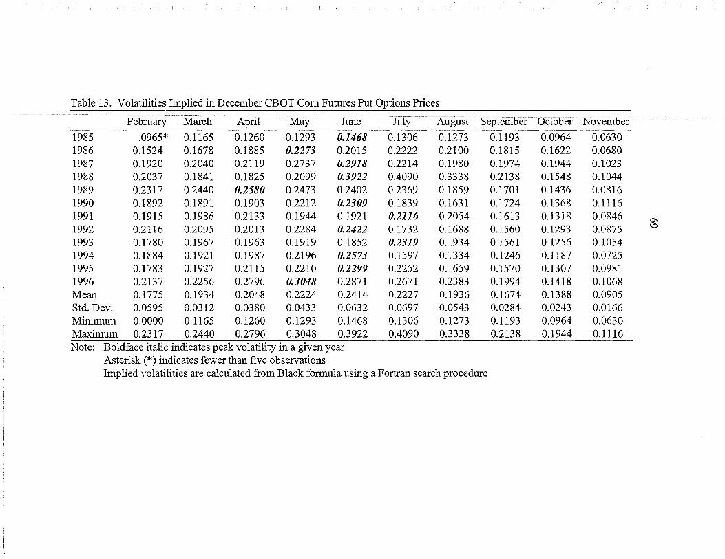
Table 13. Volatilities Implied in December CBOT Com Futures Put Options Prices

February March April May Jl.iile July August Septen1ber OCtober

1985 .0965* 0.1165 0.1260 0.1293 0.1468 0.1306 0.1273 0.1193 0.0964 0.0630 1986 0.1524 0.1678 0.1885 0.2273 0.2015 0.2222 0.2100 0.1815 0.1622 0.0680 1987 0.1920 0.2040 0.2119 0.2737 0.2918 0.2214 0.1980 0.1974 0.1944 0.1023 1988 0.2037 0.1841 0.1825 0.2099 0.3922 0.4090 0.3338 0.2138 0.1548 0.1044 1989 0.2317 0.2440 0.2580 0.2473 0.2402 0.2369 0.1859 0.1701 0.1436 0.0816 1990 0.1892 0.1891 0.1903 0.2212 0.2309 0.1839 0.1631 0.1724 0.1368 0.1116 1991 0.1915 0.1986 0.2133 0.1944 0.1921 0.2116 0.2054 0.1613 0.1318 0.0846 0\

1992 0.2116 0.2095 0.2013 0.2284 0.2422 0.1732 0.1688 0.1560 0.1293 0.0875 \0

1993 0.1780 0.1967 0.1963 0.1919 0.1852 0.2319 0.1934 0.1561 0.1256 0.1054 1994 0.1884 0.1921 0.1987 0.2196 0.2573 0.1597 0.1334 0.1246 0.1187 0.0725 1995 0.1783 0.1927 0.2115 0.2210 0.2299 0.2252 0.1659 0.1570 0.1307 0.0981 1996 0.2137 0.2256 0.2796 0.3048 0.2871 0.2671 0.2383 0.1994 0.1418 0.1068 Mean 0.1775 0.1934 0.2048 0.2224 0.2414 0.2227 0.1936 0.1674 0.1388 0.0905 Std. Dev. 0.0595 0.0312 0.0380 0.0433 0.0632 0.0697 0.0543 0.0284 0.0243 0.0166 Minimmn 0.0000 0.1165 0.1260 0.1293 0.1468 0.1306 0.1273 0.1193 0.0964 0.0630 Maximmn 0.2317 0.2440 0.2796 0.3048 0.3922 0.4090 0.3338 0.2138 0.1944 0.1116 Note: Boldface italic indicates peak volatility in a given year

Asterisk (*) indicates fewer than five observations Implied volatilities are calculated from Black formula using a Fortran search procedure

Table 14: Volatilities Implied in November CBOT Soybean Futures Call Options Prices

February March Aprif May Jtme July August September Octo bet

1985 0.1508 0.1430 0.1541 0.1564 0.1694 0.1488 0.1423 0.1136 0.0731 1986 0.1352 0.1384 0.1583 0.1626 0.1402 0.1602 0.1606 0.1072 0.0917 1987 0.1069 0.1204 0.1502 0.2268 0.2568 0.2193 0.1286 0.0957 0.0999 1988 0.1801 0.1769 0.1935 0.2257 0.3410 0.3594 0.3247 0.2142 0.1155 1989 0.2151 0.2315 0.2327 0.2109 0.2120 0.2381 0.1771 0.1534 0.1072 1990 0.1428 0.1537 0.1603 0.1762 0.1883 0.1708 0.1547 0.1270 0.0916 1991 0.1642 0.1709 0.1771 0.1661 0.1553 0.1948 0.2106 0.1626 0.0836 -..l

1992 0.1842 0.1923 0.1821 0.2140 0.2329 0.1400 0.1273 0.1232 0.1014 0

1993 0.0641 0.1697 0.1735 0.1740 0.1761 0.2714 0.1944 0.1354 0.0977 1994 0.1593 0.1589 0.1565 0.1950 0.2510 0.1543 0.1248 0.1182 0.0976 1995 0.1543 0.1210 0.1019 0.1021 0.1486 0.1260 0.0656 0.0603 0.0164 1996 0.1705 0.1663 0.2169 0.2259 0.2149 0.2067 0.1966 0.1559 0.1025 Mean 0.1523 0.1619 0.1714 0.1863 0.2072 0.1992 0.1673 0.1306 0.0899 Std. Dev. 0.0387 0.0309 0.0338 0.0374 0.0575 0.0665 0.0635 0.0386 0.0256 Minimum 0.0641 0.1204 0.1019 0.1021 0.1402 0.1260 0.0656 0.0603 0.0164 Maximum 0.2151 0.2315 0.2327 0.2268 0.3410 0.3594 0.3247 0.2142 0.1155 Note: Boldface italic indicates peale volatility in a given year

Implied volatilities are calculated from Black fonnula using a Fortran search procedure

Table 15. Volatilities hnplied in November CBOT Soybean Futures Put Options Prices

February March Apiil Ma.Y Jiuie ·July August Septe1nber October

1985 0.1505 0.1431 0.1571 0.1614 0.1784 0.1605 0.1455 0.1106 0.0737 1986 0.1414 0.1484 0.1713 0.1785 0.1528 0.1752 0.1578 0.1161 0.0670 1987 0.1091 0.1303 0.1604 0.2426 0.2712 0.2345 0.1486 0.1157 0.0997 1988 0.1871 0.1845 0.2001 0.2317 0.3390 0.3797 0.3286 0.2133 0.1212 1989 0.2170 0.2338 0.2336 0.2126 0.2179 0.2408 0.1851 0.1576 0.1024 1990 0.1530 0.1670 0.1714 0.1851 0.1973 0.1842 0.1666 0.1366 0.0857 1991 0.1696 0.1768 0.1834 0.1774 0.1702 0.2057 0.2334 0.1797 0.0931 -....l

1992 0.1878 0.2042 0.1901 0.2324 0.2507 0.1577 0.1342 0.1257 0.0523 ......

1993 0.1657 0.1783 0.1862 0.1920 0.1982 0.2802 0.2181 0.1617 0.0809 1994 0.1651 0.1698 0.1700 0.2154 0.2682 0.1677 0.1215 0.1164 0.0650 1995 0.1678 0.1836 0.1996 0.2096 0.2290 0.2270 0.1577 0.1604 0.0999 1996 0.1818 0.1820 0.2307 0.2380 0.2238 0.2159 0.2077 0.1648 0.1022 Mean 0.1663 0.1752 0.1878 0.2064 0.2247 0.2191 0.1837 0.1466 0.0869 Std. Dev. 0.0270 0.0276 0.0249 0.0271 0.0519 0.0629 0.0571 0.0317 0.0198 Minimum 0.1091 0.1303 0.1571 0.1614 0.1528 0.1577 0.1215 0.1106 0.0523 Maximum 0.2170 0.2338 0.2336 0.2426 0.3390 0.3797 0.3286 0.2133 0.1212 Note: Boldface italic indicates peak volatility in a given year

hnplied volatilities are calculated from Black formula using a Fortran search procedure

Table 16. Volatilities Implied in September CBOT Spring Wheat Futures Call Options Prices

February ··March Ap1il May June July August

1987 .1924* 0.1506 0.1533 0.2428 0.2176 0.1543 0.1165 1988 .2153* 0.2015 0.1854 0.2061 0.3794 0.3865 0.2118 1989 0.2235 0.2157 0.2126 0.2000 0.1611 0.1349 0.0894 1990 0.1379 .1399* 0.1376 0.1578 0.1241 0.1198 0.1309 1991 .1805* 0.1995 0.1913 0.1661 0.1454 0.1691 0.1404 1992 0.2479 0.2246 0.1963 0.1987 0.1805 0.1199 0.1016 1993 .1609* 0.1761 0.1790 0.1556 0.1398 0.1841 0.1143 'J

1994 .1803* 0.1706 0.1711 . 0.1839 0.1942 0.1474 0.0963 N

1995 0.0259 0.1520 0.1650 0.1873 0.2188 0.2306 0.1296 1996 0.2127 0.2029 0.2815 0.2930 0.2446 0.2057 0.1169 Mean 0.0848 0.1694 0.1873 0.1991 0.2006 0.1852 0.1248 Std. Dev. 0.1077 0.0647 0.0395 0.0419 0.0739 0.0794 0.0345 Minimum 0.0000 0.0000 0.1376 0.1556 0.1241 0.1198 0.0894 Maximum 0.2479 0.2246 0.2815 0.2930 0.3794 0.3865 0.2118 Note: Boldface italic indicates peak volatility in a given year

Asterisk(*) indicates five or fewer observations Implied volatilities are calculated from Black formula using a Fortran search procedure

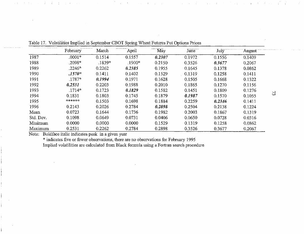
Table 17. Volatilities Implied in September CBOT Spring Wheat Futures Put Options Prices

February March. April May Jurie July August

1987 .0001 * 0.1514 0.1557 0.2307 0.1972 0.1556 0.1409 1988 .2098* .1839* .1900* 0.2150 0.3526 0.3677 0.2067 1989 .2246* 0.2262 0.2385 0.1955 0.1645 0.1378 0.0862 1990 .1570* 0.1411 0.1402 0.1529 0.1319 0.1258 0.1411 1991 .1787* 0.1994 0.1971 0.1628 0.1505 0.1668 0.1322 1992 0.2531 0.2203 0.1988 0.2010 0.1865 0.1270 0.1156 1993 .1714* 0.1723 0.1829 0.1582 0.1451 0.1809 0.1276 -....l

1994 0.1831 0.1803 0.1745 0.1879 0.1987 0.1570 0.1055 v.>

1995 ****** 0.1503 0.1698 0.1884 0.2259 0.2346 0.1411 1996 0.2143 0.2026 0.2784 0.2898 0.2504 0.2138 0.1224 Mean 0.0723 0.1644 0.1736 0.1982 0.2003 0.1867 0.1319 Std. Dev. 0.1098 0.0649 0.0731 0.0406 0.0650 0.0728 0.0316 Minimum 0.0000 0.0000 0.0000 0.1529 0.1319 0.1258 0.0862 Maximum 0.2531 0.2262 0.2784 0.2898 0.3526 0.3677 0.2067 Note: Boldface italic indicates peale in a given year

*indicates five or fewer observations, there are no observations for February 1995 Implied volatilities are calculated from Black formula using a Fortran search procedure

74

distributional assumptions ofthe Black-Scholes analysis, the implied standard deviation is

the futures options market's optimal forecast of the standard deviation of the distribution of

futures price over the discrete interval between t and T-t. It is thus necessary to look at

implied standard deviation when considering Black-Scholes assumptions and market

efficiency. The reader should note that seasonality in implied volatility is a necessary but

not sufficient condition for seasonality in implied standard deviation. As a result it is

important to look at both implied volatility and implied standard deviation when considering

Black-Scholes assumptions.

Implied Standard Deviation

The second measure of variability that is analyzed is the implied standard deviation,

which is the implied volatility times the square root of the horizon, Oj vrr- t).

As discussed in the previous section, it is important to look at implied standard

deviation in conjunction with implied volatility in order to provide a complete analysis of

Black-Scholes assumptions. If the Black-Scholes analysis were correct, then implied

standard deviation should be a monotonic decreasing function over the time span of the

. contract (or at "worst" a horizontal line given the seasonality in implied volatility).

These are shown in tables 18 through 23. Although there are instances in which the

implied standard deviation displays peaks in mid-year, it does not appear that implied

standard deviations display an overall seasonal pattern. When looking at the mean implied

standard deviation, there is a peak in June for com puts and soybean calls. These peaks are

Table 18. Com Call Implied Standard Deviation From CBOT December Com Futures Options, orV(T-t)

Februmy March Aplil May June July August September October November

1985 0.0936 * 0.1045 0.1003 0.0981 0.1047 0.0884 0.0757 0.0617 0.0410 0.0224 1986 0.1374 0:1397 0.1481 OJ737 0.14-10 0;1431 0;12.30 0.0945 0,0687 0,0075 1987 0.1699 0.1768 0.1761 0.2125 0.2066 0.1445 0.1116 0.0955 0.0780 0.0295 1988 0.2143 0.1548 0.1467 0.1586 0.2880 0.2645 0.1990 0.1067 0.0631 0.0344 1989 0.2025 0.2102 0.2109 0.1878 0.1692 0.1539 0.1037 0.0824 0.0580 0.0258 1990 0.1669 0.1584 0.1535 0.1648 0.1591 0.1182 0.0931 0.0874 0.0585 0.0288 1991 0.1691 0.1705 0.1724 0.1452 0.1367 0.1369 0.1177 0.0807 0.0517 0.0289 -.....}

1992 0.1934 0.1761 0.1617 0.1703 0.1671 0.1096 0.0973 0.0796 0.0574 0.0321 VI

1993 0.1594 0.1607 0.1521 0.1397 0.1252 0.1447 0.1057 0.0711 0.0499 0.0356 1994 0.2051 0.1625 0.1564 0.1609 0.1764 0.0976 0.0739 0.0631 0.0517 0.0327 1995 0.1565 0.1616 0.1663 0.1617 0.1583 0.1422 0.0919 0.0780 0.0543 0.0270 1996 0.1908 0.1902 0.2241 0.2303 0.2030 0.1747 0.1423 0.1000 0.0607 0.0392 Mem1 0.1716 0.1638 0.1641 0.1670 0.1696 0.1432 0.1113 0.0834 0.0577 0.0287 Std. Dev. 0.0336 0.0260 0.0316 0.0339 0.0476 0.0454 0.0337 0.0141 0.0095 0.0081 Minimmn 0.0936 0.1045 0.1003 0.0981 0.1047 0.0884 0.0739 0.0617 0.0410 0.0075 Maximmn 0.2143 0.2102 0.2241 0.2303 0.2880 0.2645 0.1990 0.1067 0.0780 0.0392 Note: Boldface italic indicates peale in a given year

Astelisk (*) indicates fewer than five observations

Table 19. Com Put Implied Standard Deviation From December CBOT Com Futures Options, a1V(T-t)

February March April May Jtme July August September October November

1985 .0888* 0.1020 0.1041 0.1002 0.1054 0.0859 0.0751 0.0612 0.0410 0.0195 1986 0.1402 0.1470 0.1557 0.1761 0.1446 0.1462 0.1239 0.0931 0.0690 0.0211 1987 0.1767 0.1787 0.1750 0.2120 0.2094 0.1457 0.1168 0.1012 0.0827 0.0317 1988 0.1874 0.1613 0.1507 0.1626 0.2815 0.2691 0.1969 0.1096 0.0658 0.0323 1989 0.2132 0.2137 0.2131 0.1916 0.1724 0.1559 0.1097 0.0872 0.0611 0.0253 1990 0.1741 0.1656 0.1572 0.1713 0.1657 0.1210 0.0962 0.0884 0.0582 0.0346 1991 0.1762 0.1740 0.1762 0.1506 0.1379 0.1392 0.1212 0.0827 0.0560 0.0262 ---1

1992 0.1947 0.1835 0.1663 0.1769 0.1738 0.1139 0.0996 0.0800 0.0550 0.0271 0\

1993 0.1638 0.1723 0.1621 0.1486 0.1329 0.1526 0.1141 0.0800 0.0534 0.0326 1994 0.1733 0.1683 0.1641 0.1701 0.1847 0.1051 0.0787 0.0639 0.0505 0.0225 1995 0.1641 0.1688 0.1747 0.1712 0.1650 0.1482 0.0979 0.0805 0.0556 0.0304 1996 0.1966 0.1976 0.2309 0.2361 0.2061 0.1757 0.1406 0.1023 0.0603 0.0331 Mean 0.1708 0.1694 0.1692 0.1723 0.1733 0.1465 0.1142 0.0858 0.059 0.028 Std. Dev. 0.0318 0.0273 0.0314 0.0336 0.0454 0.0459 0.0321 0.0146 0.0103 0.0051 Minimum 0.0888 0.102 0.1041 0.1002 0.1054 0.0859 0.0751 0.0612 0.041 0.0195 Maximum 0.2132 0.2137 0.2309 0.2361 0.2815 0.2691 0.1969 0.1096 0.0827 0.0346 Note: Boldface italic indicates peak in a given year

Asterisk (*) indicates fewer than five observations

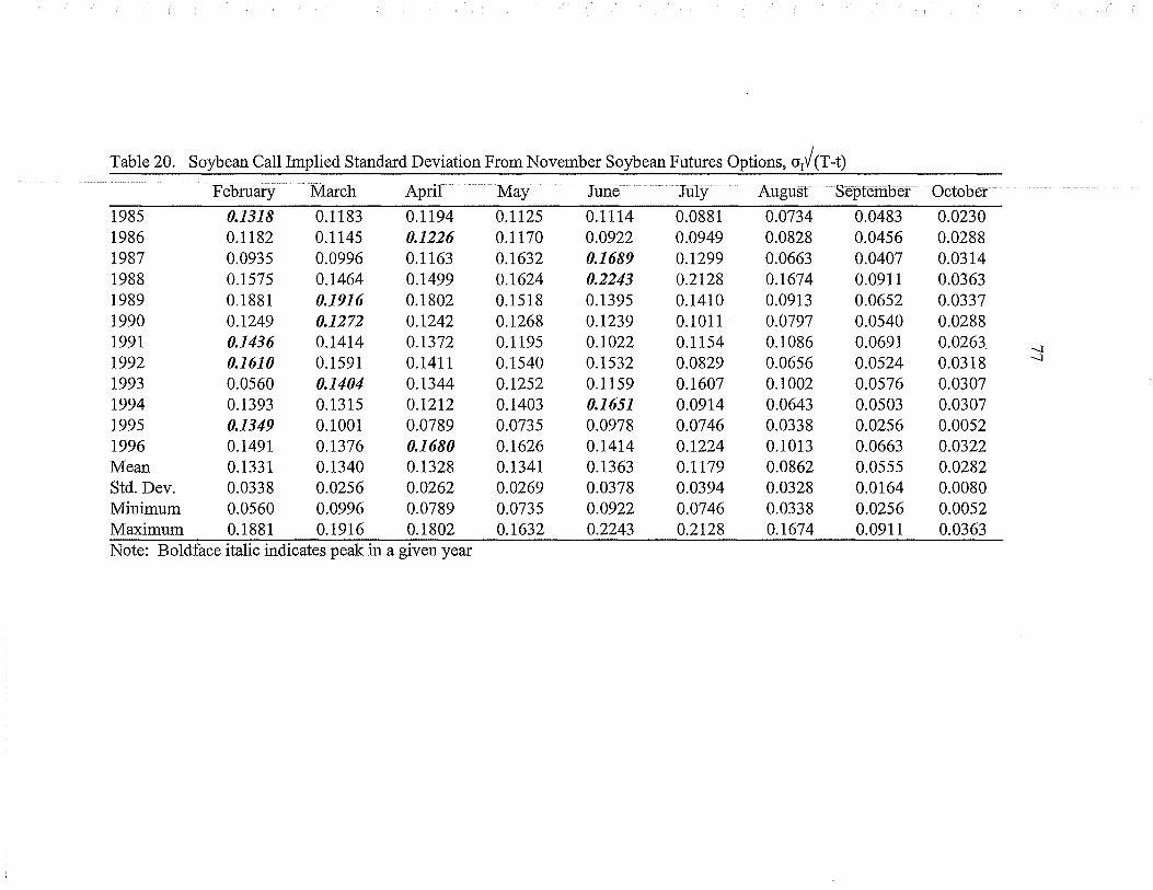
Table 20. Soybean Call Implied Standard Deviation From November Soybean Futures Options, a1V (T -t)

Februa1y March April May Jl.l.Ile July August September October

1985 0.1318 0.1183 0.1194 0.1125 0.1114 0.0881 0.0734 0.0483 0.0230 1986 0.1182 0.1145 0.1226 0.1170 0.0922 0.0949 0.0828 0.0456 0.0288 1987 0.0935 0.0996 0.1163 0.1632 0.1689 0.1299 0.0663 0.0407 0.0314 1988 0.1575 0.1464 0.1499 0.1624 0.2243 0.2128 0.1674 0.0911 0.0363 1989 0.1881 0.1916 0.1802 0.1518 0.1395 0.1410 0.0913 0.0652 0.0337 1990 0.1249 0.1272 0.1242 0.1268 0.1239 0.1011 0.0797 0.0540 0.0288 1991 0.1436 0.1414 0.1372 0.1195 0.1022 0.1154 0.1086 0.0691 0.0263. .........

1992 0.1610 0.1591 0.1411 0.1540 0.1532 0.0829 0.0656 0.0524 0.0318 .........

1993 0.0560 0.1404 0.1344 0.1252 0.1159 0.1607 0.1002 0.0576 0.0307 1994 0.1393 0.1315 0.1212 0.1403 0.1651 0.0914 0.0643 0.0503 0.0307 1995 0.1349 0.1001 0.0789 0.0735 0.0978 0.0746 0.0338 0.0256 0.0052 1996 0.1491 0.1376 0.1680 0.1626 0.1414 0.1224 0.1013 0.0663 0.0322 Mean 0.1331 0.1340 0.1328 0.1341 0.1363 0.1179 0.0862 0.0555 0.0282 Std. Dev. 0.0338 0.0256 0.0262 0.0269 0.0378 0.0394 0.0328 0.0164 0.0080 Minimum 0.0560 0.0996 0.0789 0.0735 0.0922 0.0746 0.0338 0.0256 0.0052 Maximum 0.1881 0.1916 0.1802 0.1632 0.2243 0.2128 0.1674 0.0911 0.0363 Note: Boldface italic indicates peak in a given year

Table 21. Soybean Put Implied Standard Deviation From November CBOT Soybean Futures Options, a/ (T -t)

Februar)r March April May June July August September October

1985 0.1316 0.1184 0.1217 0.1161 0.1174 0.0950 0.0750 0.0470 0.0231 1986 0.1236 0.1228 0.1327 0.1284 0.1005 0.1038 0.0813 0.0494 0.0210 1987 0.0954 0.1078 0.1242 0.1746 0.1784 0.1389 0.0766 0.0492 0.0313 1988 0.1636 0.1527 0.1550 0.1667 0.2230 0.2249 0.1694 0.0907 0.0381 1989 0.1897 0.1935 0.1809 0.1530 0.1434 0.1426 0.0954 0.0670 0.0322 1990 0.1338 0.1382 0.1328 0.1332 0.1298 0.1091 0.0859 0.0581 0.0269 1991 0.1483 0.1463 0.1421 0.1277 0.1120 0.1218 0.1203 0.0764 0.0292 ......:)

1992 0.1642 0.1690 0.1473 0.1672 0.1649 0.0934 0.0692 0.0534 0.0164 00

1993 0.1449 0.1476 0.1442 0.1382 0.1304 0.1659 0.1124 0.0688 0.0254 1994 0.1443 0.1405 0.1317 0.1550 0.1764 0.0993 0.0626 0.0495 0.0204 1995 0.1467 0.1519 0.1546 0.1508 0.1507 0.1344 0.0813 0.0682 0.0314 1996 0.1589 0.1506 0.1787 0.1713 0.1472 0.1279 0.1071 0.0701 0.0321 Mean 0.1454 0.1450 0.1455 0.1485 0.1478 0.1297 0.0947 0.0623 0.0273 Std. Dev. 0.0236 0.0228 0.0193 0.0195 0.0341 0.0372 0.0294 0.0135 0.0062 Minimum 0.0954 0.1078 0.1217 0.1161 0.1005 0.0934 0.0626 0.0470 0.0164 Maximum 0.1897 0.1935 0.1809 0.1746 0.2230 0.2249 0.1694 0.0907 0.0381 Note: Boldface italic indicates peak in a given year

Table 22. Spring Wheat Call Implied Standard Deviation From September CBOT Spring Wl1eat Futures Options, a/(T-t)

February March April May Jtme July August

1987 .1487* 0.1084 0.1009 0.1438 0.1122 0.0661 0.0366 1988 .1664* 0.1450 0.1220 0.1221 0.1956 0.1656 0.0665 1989 0.1727 0.1552 0.1399 0.1184 0.0830 0.0578 0.0281 1990 0.1066 .1007* 0.0905 0.0934 0.0640 0.0513 0.0411 1991 .1395* 0.1436 0.1259 0.0984 0.0750 0.0724 0.0441 1992 0.1916 0.1616 0.1291 0.1177 0.0930 0.0514 0.0319 1993 .1243* 0.1267 0.1178 0.0921 0.0721 0.0789 0.0359 -....l

1994 .1393* 0.1228 0.1126 0.1089 0.1001 0.0631 0.0302 \0

1995 0.0200 0.1094 0.1086 0.1109 0.1128 0.0988 0.0407 1996 0.1644 0.1460 0.1852 0.1735 0.1261 0.0881 0.0367 Mean 0.1374 0.1319 0.1232 0.1179 0.1034 0.0794 0.0392 Std. Dev. 0.0481 0.0213 0.0260 0.0248 0.0381 0.0340 0.0108 Minimum 0.0200 0.1007 0.0905 0.0921 0.0640 0.0513 0.0281 Maximum 0.1916 0.1616 0.1852 0.1735 0.1956 0.1656 0.0665 Note: Boldface italic indicates peale in a given year

Asterisk (*) indicates five or fewer observations

Table 23. Spring Wheat Put Implied Standard Deviation From September CBOT Spring Wheat Futures Options, a1V(T-t)

February March April May Jfuie July August

1987 .00008* 0.1089 0.1024 0.1366 0.1017 0.0666 0.0443 1988 .1621 * .1323* .1250* 0.1273 0.1818 0.1574 0.0649 1989 .1736* 0.1628 0.1569 0.1158 0.0848 0.0590 0.0271 1990 .1213* 0.1015 0.0922 0.0905 0.0680 0.0539 0.0443 1991 .1381 * 0.1435 0.1297 0.0964 0.0776 0.0714 0.0415 1992 0.1956 0.1585 0.1308 0.1190 0.0961 0.0544 0.0363 1993 .1325* 0.1240 0.1203 0.0937 0.0748 0.0775 0.0401 00

1994 0.1415 0.1297 0.1148 0.1113 0.1024 0.0672 0.0331 0

1995 ****** 0.1082 0.1117 0.1116 0.1165 0.1005 0.0443 1996 0.1656 0.1458 0.1832 0.1716 0.1291 0.0915 0.0384 Mean 0.1538 0.1315 0.1267 0.1174 0.1033 0.0799 0.0414 Std. Dev. 0.0247 0.0213 0.0265 0.0241 0.0335 0.0312 0.0099 Minimum 0.1213 0.1015 0.0922 0.0905 0.068 0.0539 0.0271 Maximum 0.1956 0.1628 0.1832 0.1716 0.1818 0.1574 0.0649 Note: Boldface italic indicates peale in a given year

Asterisk (*) indicates five or fewer observations February 1987 is not used in summary statistic calculations There are no observations for February 1995

81

not significantly different from those in earlier months when considering a standard deviation

of about .03 for both crops.

Overall, it cannot be concluded that there is significant evidence for seasonality in

standard deviations implied in com, soybean, and spring wheat futures options. Although

evidence strongly supports seasonality in implied volatility, it appears that the market is

"correcting" such seasonality through the implied standard deviation.

Relationship Between Put and Call Implied Volatilities

It is suspected that implied volatilities from puts and calls on the same futures

contract should be highly correlated. If not, then potential arbitrage opportunities exist,

which would force the put and call markets back into equilibrium. Implied volatilities from

calls are regressed on those from puts using OLS estimation of the following empirical form:

Implied Call = a + PUmplied Put)

Results are summarized in table 24 below:

Table 24: Relationship between Put and Call CBOT Futures Options Implied Volatilities

Com

-.00002 (-.0074) .9786*

(71.9559) T-statistic for P*1 -1.5735 R-Square .9778 Note: T -values are shown in parentheses

Soybeans

.0031 (.3735) .9007*

(20.2860) -2.2365*

.7950

* denotes significance at the 5 % level for a two-tailed test

Wheat

-.0155 (-3.9744) 1.0738*

(52.3805) 3.6000* .9794

Sample sizes used are 120, 108, and 60 respectively for com, soybeans, and wheat

82

While com and spring wheat implied volatilities appear to be very highly correlated,

soybean seems surprisingly low. The estimated beta for all three crops, however, is strongly

significant. When considering a test of p * 1, it is interesting to note that beta appears to be

significantly different from one for soybeans and wheat.

Levels oflrnplied Volatilities and Price Changes

Tables 25 through 27 show estimated call implied volatilities, put implied volatilities,

and ln( ep/bp ), which is used as a measure of change between the average monthly futures

price and the ending price. These are the relevant data for put and call implied volatilities

and commodity futures price changes between beginning and ending periods which are

ultimately used to test whether futures options prices are accurate predictors of futures price

changes by means of estimated implied volatilities.

Table 25. Com Implied Volatilities and Futures Price Changes Measured by Ln (ep/bp) February

1985 1986 1987 1988 1989 1990 1991 1992 1993 1994 1995 1996 Mean Std. Dev. Minimum Maximum

Call Implied Volatility

0.1017 0.1493 0.1847 0.2329 0.2201 0.1814 0.1838 0.2102 0.1732 0.2229 0.1701 0.2074 0.1865 0.0365 0.1017 0.2329

Put Implied Volatility

0.0965 0.1524 0.1920 0.2037 0.2317 0.1892 0.1915 0.2116 0.1780 0.1884 0.1783 0.2137 0.1856 0.0346 0.0965 0.2317

Ln(ep/bp)

0.0674 0.3309 0.0599 0.2089 0.1487 0.0994 0.0304 0.2518 0.1896 0.2022 0.2900 0.1351 0.1679 0.0947 0.0304 0.3309

83

Table 25 (cont.) March

Com Implied Volatility Put Implied Volatility Ln(ep/bp)

1985 0.1193 0.1165 0.0612 1986 0.1595 0.1678 0.3127 1987 0.2019 0.2040 0.0347 1988 0.1767 0.1841 0.1998 1989 0.2400 0.2440 0.1465 1990 0.1808 0.1891 0.1289 1991 0.1947 0.1986 0.0414 1992 0.2010 0.2095 0.2407 1993 0.1835 0.1967 0.1769 1994 0.1855 0.1921 0.1823 1995 0.1845 0.1927 0.2782 1996 0.2171 0.2256 0.1558 Mean 0.1870 0.1934 0.1633 Std.Dev. 0.0297 0.0312 0.0888 Minimum 0.1193 0.1165 0.0347 Maximum 0.2400 0.2440 0.3127

April

Com Implied Volatility Put Implied Volatility Ln(ep/bp)

1985 0.1215 0.1260 0.0737 1986 0.1793 0.1885 0.2769 1987 0.2132 0.2119 0.0130 1988 0.1776 0.1825 0.1706 1989 0.2554 0.2580 0.1171 1990 0.1859 0.1903 0.1674 1991 0.2088 0.2133 0.0352 1992 0.1958 0.2013 0.1874 1993 0.1842 0.1963 0.1720 1994 0.1894 0.1987 0.1518 1995 0.2013 0.2115 0.2670 1996 0.2714 0.2796 0.2094 Mean 0.1987 0.2048 0.1535 Std. Dev. 0.0382 0.0380 0.0824 Minimum 0.1215 0.1260 0.0130 Maximum 0.2714 0.2796 0.2769

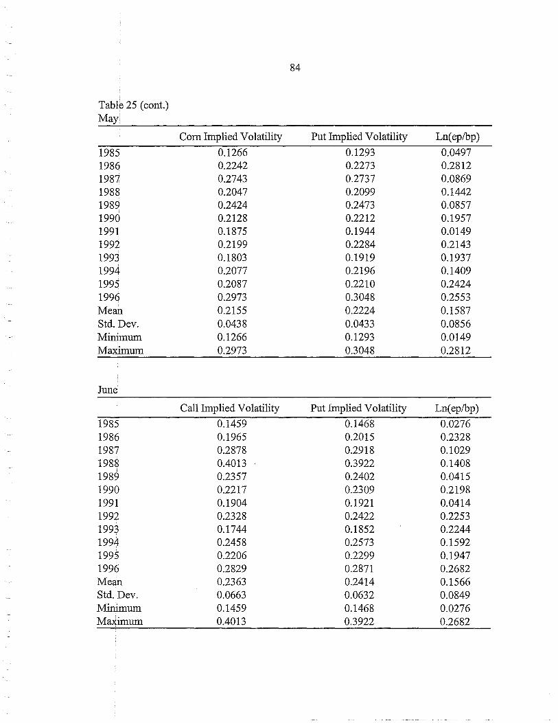
84

Table 25 (cont.) May

Com Implied Volatility Put Implied Volatility Ln(ep/bp)

1985 0.1266 0.1293 0.0497 1986 0.2242 0.2273 0.2812 1987 0.2743 0.2737 0.0869 1988 0.2047 0.2099 0.1442 1989 0.2424 0.2473 0.0857 1990 0.2128 0.2212 0.1957 1991 0.1875 0.1944 0.0149 1992 0.2199 0.2284 0.2143 1993 0.1803 0.1919 0.1937 1994 0.2077 0.2196 0.1409 1995 0.2087 0.2210 0.2424 1996 0.2973 0.3048 0.2553 Mean 0.2155 0.2224 0.1587 Std. Dev. 0.0438 0.0433 0.0856 Minimum 0.1266 0.1293 0.0149 Maximum 0.2973 0.3048 0.2812

June

Call Implied Volatility Put Implied Volatility Ln(ep/bp)

1985 0.1459 0.1468 0.0276 1986 0.1965 0.2015 0.2328 1987 0.2878 0.2918 0.1029 1988 0.4013 0.3922 0.1408 1989 0.2357 0.2402 0.0415 1990 0.2217 0.2309 0.2198 1991 0.1904 0.1921 0.0414 1992 0.2328 0.2422 0.2253 1993 0.1744 0.1852 0.2244 1994 0.2458 0.2573 0.1592 1995 0.2206 0.2299 0.1947 1996 0.2829 0.2871 0.2682 Mean 0.2363 0.2414 0.1566 Std.Dev. 0.0663 0.0632 0.0849 Minimum 0.1459 0.1468 0.0276 Maximum 0.4013 0.3922 0.2682

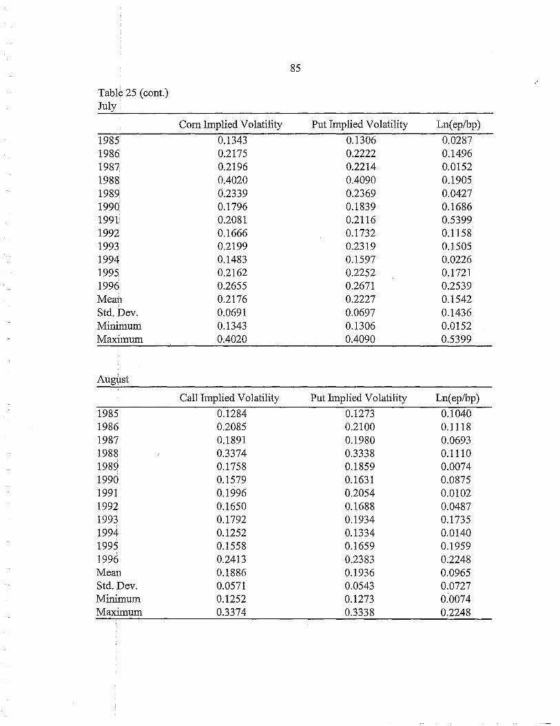
85 I

Table 25 (cont.) July

Com Implied Volatility Put Implied Volatility Ln(ep/bp)

1985 0.1343 0.1306 0.0287 1986 0.2175 0.2222 0.1496 1987 0.2196 0.2214 0.0152 1988 0.4020 0.4090 0.1905 1989 0.2339 0.2369 0.0427 1990 0.1796 0.1839 0.1686 1991 0.2081 0.2116 0.5399 1992 0.1666 0.1732 0.1158 1993 0.2199 0.2319 0.1505 1994 0.1483 0.1597 0.0226 1995 0.2162 0.2252 0.1721 1996 0.2655 0.2671 0.2539 Mean 0.2176 0.2227 0.1542 Std. Dev. 0.0691 0.0697 0.1436 Minimum 0.1343 0.1306 0.0152 Maximum 0.4020 0.4090 0.5399

August

Call Implied Volatility Put Implied Volatility Ln(ep/bp)

1985 0.1284 0.1273 0.1040 1986 0.2085 0.2100 0.1118 1987 0.1891 0.1980 0.0693 1988 0.3374 0.3338 0.1110 1989 0.1758 0.1859 0.0074 1990 0.1579 0.1631 0.0875 1991 0.1996 0.2054 0.0102 1992 0.1650 0.1688 0.0487 1993 0.1792 0.1934 0.1735 1994 0.1252 0.1334 0.0140 1995 0.1558 0.1659 0.1959 1996 0.2413 0.2383 0.2248 Mean 0.1886 0.1936 0.0965 Std. Dev. 0.0571 0.0543 0.0727 Minimum 0.1252 0.1273 0.0074 Maximum 0.3374 0.3338 0.2248

86

Table 25 (cont.) September

Call hnplied Volatility Put hnplied Volatility Ln(eplbp)

1985 0.1204 0.1193 0.1181 1986 0.1842 0.1815 0.0963 1987 0.1863 0.1974 0.0242 1988 0.2081 0.2138 0.0935 1989 0.1606 0.1701 0.0046 1990 0.1705 0.1724 0.0241 1991 0.1574 0.1613 0.0010 1992 0.1552 0.1560 0.0370 1993 0.1386 0.1561 0.1858 1994 0.1230 0.1246 0.0060 1995 0.1521 0.1570 0.1253 1996 0.1950 0.1994 0.1717 Mean 0.1626 0.1674 0.0740 Std. Dev. 0.0275 0.0284 0.0665 Minimum 0.1204 0.1193 0.0010 Maximum 0.2081 0.2138 0.1858

October

Call hnplied Volatility Put hnplied Volatility Ln(eplbp)

1985 0.0964 0.0964 0.1023 1986 0.1615 0.1622 0.1131 1987 0.1835 0.1944 0.0197 1988 0.1485 0.1548 0.0779 1989 0.1363 0.1436 0.0242 1990 0.1376 0.1368 0.0255 1991 0.1215 0.1318 0.0015 1992 0.1350 0.1293 0.0065 1993 0.1173 0.1256 0.1532 1994 0.1216 0.1187 0.0140 1995 0.1276 0.1307 0.0612 1996 0.1427 0.1418 0.0517 Mean 0.1358 0.1388 0.0542 Std.nev. 0.0224 0.0243 0.0484 Minimum 0.0964 0.0964 0.0015 Maximum 0.1835 0.1944 0.1532

87

Table 25 (cont.) November

Com Implied Volatility Put Implied Volatility Ln(ep/bp)

1985 0.0724 0.0630 0.0384 1986 0.0241 0.0680 0.1193 1987 0.0952 0.1023 0.0213 1988 0.1110 0.1044 0.0093 1989 0.0832 0.0816 0.0189 1990 0.0931 0.1116 0.0097 1991 0.0933 0.0846 0.0315 1992 0.1036 0.0875 0.0075 1993 0.1149 0.1054 0.0565 1994 0.1057 0.0725 0.0152 1995 0.0873 0.0981 0.0454 1996 0.1267 0.1068 0.0054 Mean 0.0925 0.0905 0.0315 Std. Dev. 0.0261 0.0166 0.0321 Minimum 0.0241 0.0630 0.0054 Maximum 0.1267 0.1116 0.1193

Table 26. Soybean Implied Volatilities and Futures Price Change Measured by Ln ( ep/bp) February

Call Implied Volatility Put Implied Volatility Ln(ep/bp)

1985 0.1508 0.1505 0.2106 1986 0.1352 0.1414 0.0425 1987 0.1069 0.1091 0.1858 1988 0.1801 0.1871 0.1238 1989 0.2151 0.2170 0.2301 1990 0.1428 0.1530 0.0667 1991 0.1642 0.1696 0.0842 1992 0.1842 0.1878 0.0752 1993 0.0641 0.1657 0.1545 1994 0.1593 0.1651 0.1434 1995 0.1543 0.1678 0.1541 1996 0.1705 0.1818 0.0239 Mean 0.1523 0.1663 0.1246 Std. Dev. 0.0387 0.0270 0.0665 Minimum 0.0641 0.1091 0.0239 Maximum 0.2151 0.2170 0.2301

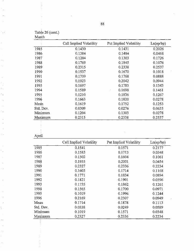
88

Table 26 (cont.) March

Call Implied Volatility Put Implied Volatility Ln(ep/bp)

1985 0.1430 0.1431 0.2026 1986 0.1384 0.1484 0.0468 1987 0.1204 0.1303 0.1726 1988 0.1769 0.1845 0.1076 1989 0.2315 0.2338 0.2537 1990 0.1537 0.1670 0.1018 1991 0.1709 0.1768 0.0888 1992 0.1923 0.2042 0.0944 1993 0.1697 0.1783 0.1343 1994 0.1589 0.1698 0.1461 1995 0.1210 0.1836 0.1267 1996 0.1663 0.1820 0.0278 Mean 0.1619 0.1752 0.1253 Std .. Dev. 0.0309 0.0276 0.0633 Minimum 0.1204 0.1303 0.0278 Maximum 0.2315 0.2338 0.2537

April

Call Implied Volatility Put Implied Volatility Ln(ep/bp)

1985 0.1541 0.1571 0.2177 1986 0.1583 0.1713 0.0348 1987 0.1502 0.1604 0.1061 1988 0.1935 0.2001 0.0454 1989 0.2327 0.2336 0.2234 1990 0.1603 0.1714 0.1168 1991 0.1771 0.1834 0.0894 1992 0.1821 0.1901 0.0596 1993 0.1735 0.1862 0.1261 1994 0.1565 0.1700 0.0971 1995 0.1019 0.1996 0.1244 1996 0.2169 0.2307 0.0949 Mean 0.1714 0.1878 0.1113 Std. Dev. 0.0338 0.0249 0.0589 Minimum 0.1019 0.1571 0.0348 Maximum 0.2327 0.2336 0.2234

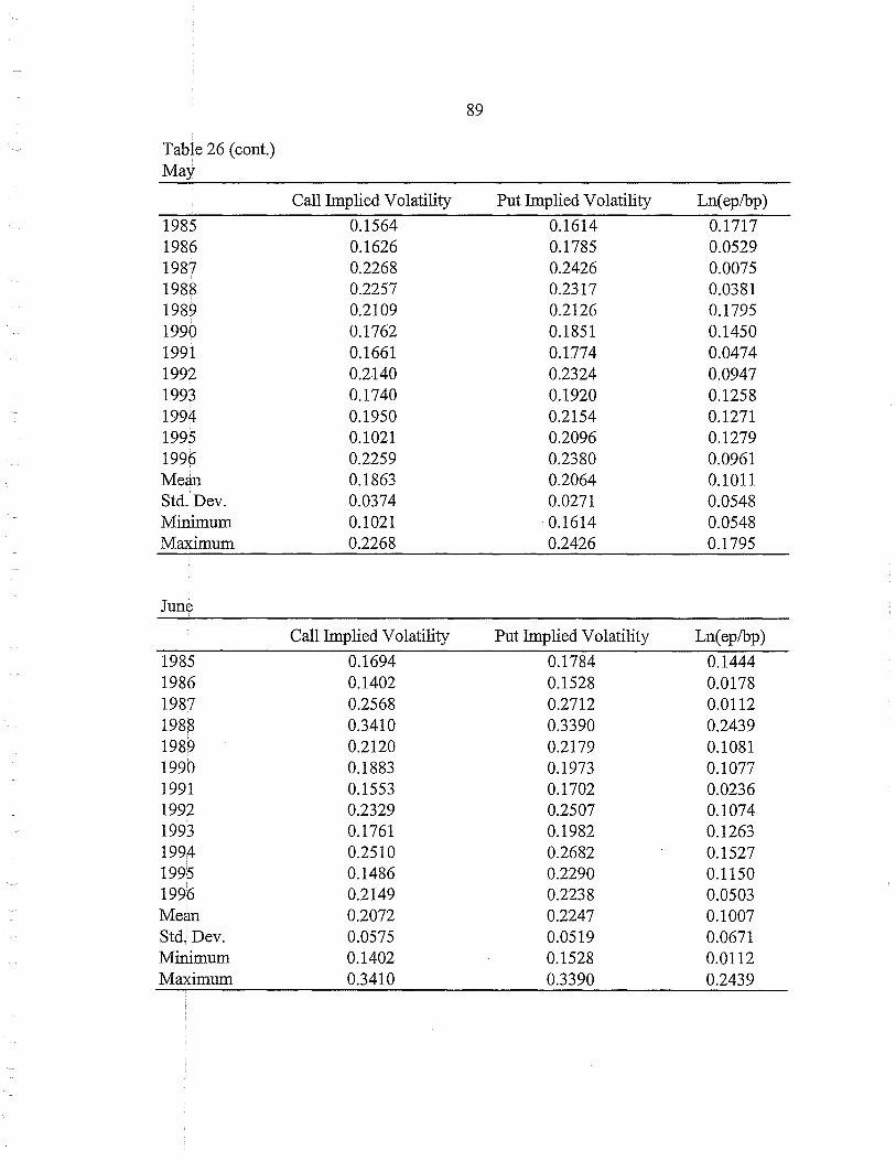
89

Table 26 (cont.) May

Call hnplied Volatility Put hnplied Volatility Ln(ep/bp)

1985 0.1564 0.1614 0.1717 1986 0.1626 0.1785 0.0529 1987 0.2268 0.2426 0.0075 1988 0.2257 0.2317 0.0381 1989 0.2109 0.2126 0.1795 1990 0.1762 0.1851 0.1450 1991 0.1661 0.1774 0.0474 1992 0.2140 0.2324 0.0947 1993 0.1740 0.1920 0.1258 1994 0.1950 0.2154 0.1271 1995 0.1021 0.2096 0.1279 1996 0.2259 0.2380 0.0961 Mean 0.1863 0.2064 0.1011 Std.Dev. 0.0374 0.0271 0.0548 Minimum 0.1021 0.1614 0.0548 Maximum 0.2268 0.2426 0.1795

June

Call hnplied Volatility Put hnplied Volatility Ln(eplbp)

1985 0.1694 0.1784 0.1444 1986 0.1402 0.1528 0.0178 1987 0.2568 0.2712 0.0112 1988 0.3410 0.3390 0.2439 1989 0.2120 0.2179 0.1081 1990 0.1883 0.1973 0.1077 1991 0.1553 0.1702 0.0236 1992 0.2329 0.2507 0.1074 1993 0.1761 0.1982 0.1263 1994 0.2510 0.2682 0.1527 1995 0.1486 0.2290 0.1150 1996 0.2149 0.2238 0.0503 Mean 0.2072 0.2247 0.1007 Std: Dev. 0.0575 0.0519 0.0671 Minimum 0.1402 0.1528 0.0112 Maximum 0.3410 0.3390 0.2439

90

Table 26 (cont.) July

Call hnplied Volatility Put hnplied Volatility Ln(ep/bp)

1985 0.1488 0.1605 0.1209 1986 0.1602 0.1752 0.0097 1987 0.2193 0.2345 0.0702 1988 0.3594 0.3797 0.1868 1989 0.2381 0.2408 0.0995 1990 0.1708 0.1842 0.1156 1991 0.1948 0.2057 0.0322 1992 0.1400 0.1577 0.0199 1993 0.2714 0.2802 0.0332 1994 0.1543 0.1677 0.0222 1995 0.1260 0.2270 0.0796 1996 0.2067 0.2159 0.0653 Mean 0.1992 0.2191 0.0713 Std.Dev. 0.0665 0.0629 0.0526 Minimum 0.1260 0.1577 0.0097 Maximum 0.3594 0.3797 0.1868

August

Call hnplied Volatility Put hnplied Volatility Ln(ep/bp)

1985 0.1423 0.1455 0.0500 1986 0.1606 0.1578 0.0379 1987 0.1286 0.1486 0.1174 1988 0.3247 0.3286 0.1696 1989 0.1771 0.1851 0.0066 1990 0.1547 0.1666 0.1075 1991 0.2106 0.2334 0.0246 1992 0.1273 0.1342 0.0327 1993 0.1944 0.2181 0.0176 1994 0.1248 0.1215 0.0072 1995 0.0656 0.1577 0.1173 1996 0.1966 0.2077 0.0907 Mean 0.1673 0.1837 0.0649 Std. Dev. 0.0635 0.0571 0.0535 Minimum 0.0656 0.1215 0.0066 Maximum 0.3247 0.3286 0.1696

91

Table 26 (cont.) Sepfember

Call Implied Volatility Put Implied Volatility Ln(ep/bp)

1985 0.1136 0.1106 0.0425 1986 0.1072 0.1161 0.0297 1987 0.0957 0.1157 0.0788 1988 0.2142 0.2133 0.1634 1989 0.1534 0.1576 0.0028 1990 0.1270 0.1366 0.1156 1991 0.1626 0.1797 0.0496 1992 0.1232 0.1257 0.0266 1993 0.1354 0.1617 0.0687 1994 0.1182 0.1164 0.0017 1995 0.0603 0.1604 0.0662 1996 0.1559 0.1648 0.1181 Mean 0.1306 0.1466 0.0636 Std. Dev. 0.0386 0.0317 0.0492 Minimum 0.0603 0.1106 0.0017 Maximum 0.2142 0.2133 0.1634

October

Call Implied Volatility Put Implied Volatility Ln(ep/bp)

1985 0.0731 0.0737 0.0280 1986 0.0917 0.0670 0.0253 1987 0.0999 0.0997 0.0531 1988 0.1155 0.1212 . 0.0853 1989 0.1072 0.1024 0.0239 1990 0.0916 0.0857 0.0937 1991 0.0836 0.0931 0.0096 1992 0.1014 0.0523 0.0442 1993 0.0977 0.0809 0.1063 1994 0.0976 0.0650 0.0373 1995 0.0164 0.0999 0.0392 1996 0.1025 0.1022 0.0021 Mean 0.0869 0.0869 0.0457 Std. Dev. 0.0198 0.0198 0.0332 Minimum 0.0523 0.0523 0.0021 Maximum 0.1212 0.1212 0.1063

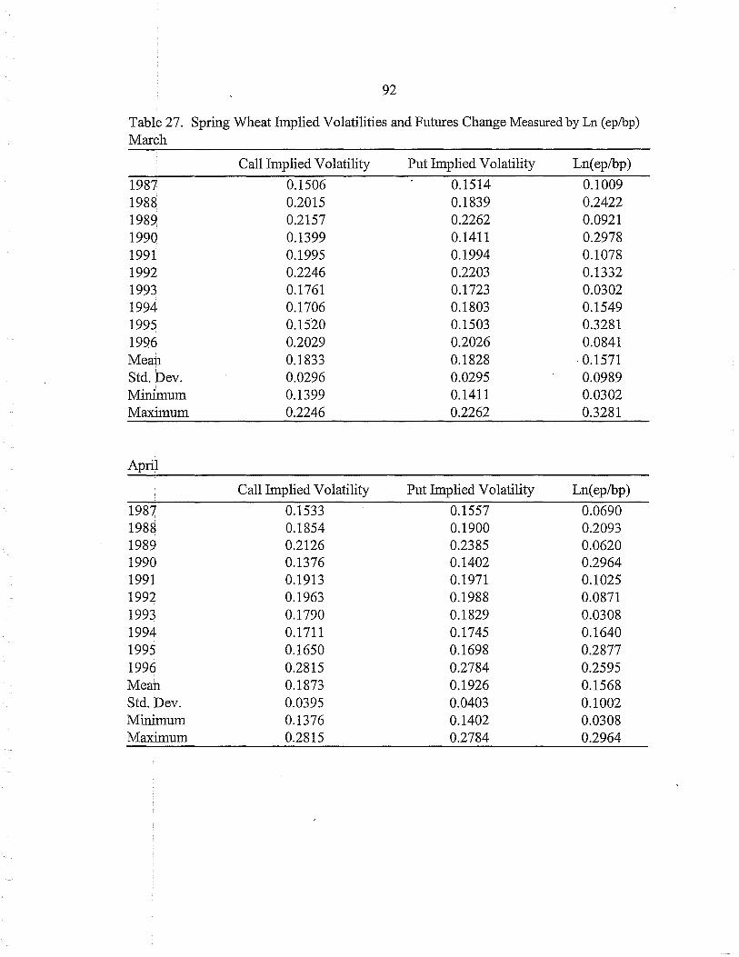
92

Table 27. Spring Wheat Implied Volatilities and Futures Change Measured by Ln ( ep/bp) March

Call Implied Volatility Put Implied Volatility Ln(ep/bp)

1987 0.1506 0.1514 0.1009 1988 0.2015 0.1839 0.2422 1989 0.2157 0.2262 0.0921 1990 0.1399 0.1411 0.2978 1991 0.1995 0.1994 0.1078 1992 0.2246 0.2203 0.1332 1993 0.1761 0.1723 0.0302 1994 0.1706 0.1803 0.1549 1995 0.1520 0.1503 0.3281 1996 0.2029 0.2026 0.0841 Mean 0.1833 0.1828 0.1571 Std. Dev. 0.0296 0.0295 0.0989 Minimum 0.1399 0.1411 0.0302 Maximum 0.2246 0.2262 0.3281

April

Call Implied Volatility Put Implied Volatility Ln(ep/bp)

1987 0.1533 0.1557 0.0690 1988 0.1854 0.1900 0.2093 1989 0.2126 0.2385 0.0620 1990 0.1376 0.1402 0.2964 1991 0.1913 0.1971 0.1025 1992 0.1963 0.1988 0.0871 1993 0.1790 0.1829 0.0308 1994 0.1711 0.1745 0.1640 1995 0.1650 0.1698 0.2877 1996 0.2815 0.2784 0.2595 Mean 0.1873 0.1926 0.1568 Std. Dev. 0.0395 0.0403 0.1002 Minimum 0.1376 0.1402 0.0308 Maximum 0.2815 0.2784 0.2964

93

Table 27 (cont.) May

Call Implied Volatility Put Implied Volatility Ln(ep/bp)

1987 0.2428 0.2307 0.0127 1988 0.2061 0.2150 0.1928 1989 0.2000 0.1955 0.0816 1990 0.1578 0.1529 0.2974 1991 0.1661 0.1628 0.1089 1992 0.1987 0.2010 0.0895 1993 0.1556 0.1582 0.0216 1994 0.1839 0.1879 0.1486 1995 0.1873 0.1884 0.2460 1996 . 0.2930 0.2898 0.2934 Mean 0.1991 0.1982 0.1493 Std. Dev. 0.0419 0.0406 0.1047 Minimum 0.1556 0.1529 0.0127 Maximum 0.2930 0.2898 0.2974

June

Call Implied Volatility Put Implied Volatility Ln(ep/bp)

1987 0.2176 0.1972 0.0648 1988 0.3794 0.3526 0.0488 1989 0.1611 0.1645 0.0544 1990 0.1241 0.1319 0.2699 1991 0.1454 0.1505 0.1312 1992 0.1805 0.1865 0.0900 1993 0.1398 0.1451 0.0513 1994 0.1942 0.1987 0.1364 1995 0.2188 0.2259 0.1590 1996 0.2446 0.2504 0.1723 Mean 0.2006 0.2003 0.1178 Std. Dev. 0.0739 0.0650 0.0708 Minimum 0.1241 0.1319 0.0488 Maximum 0.3794 0.3526 0.2699

94

Table 27 (cont.) July

Call Implied Volatility Put Implied Volatility Ln(ep/bp)

1987 0.1543 0.1556 0.0935 1988 0.3865 0.3677 0.0527 1989 0.1349 0.1378 0.0387 1990 0.1198 0.1258 0.1826 1991 0.1691 0.1668 0.1852 1992 0.1199 0.1270 0.0217 1993 0.1841 0.1809 0.0063 1994 0.1474 0.1570 0.1699 1995 0.2306 0.2346 0.0570 1996 0.2057 0.2138 0.1069 Mean 0.1852 0.1867 0.0915 Std. Dev. 0.0794 0.0728 0.0676 Minimum 0.1198 0.1258 0.0063 Maximum 0.3865 0.3677 0.1852

August

Call Implied Volatility Put Implied Volatility Ln(ep/bp)

1987 0.1165 0.1409 0.0732 1988 0.2118 0.2067 0.0481 1989 0.0894 0.0862 0.0305 1990 0.1309 0.1411 0.0849 1991 0.1404 0.1322 0.1154 1992 0.1016 0.1156 0.0582 1993 0.1143 0.1276 0.0185 1994 0.0963 0.1055 0.1075 1995 0.1296 0.1411 0.0823 1996 0.1169 0.1224 0.0745 Mean 0.1248 0.1319 0.0693 Std. :Dev. 0.0345 0.0316 0.0311 Minimum 0.0894 0.0862 0.0185 Maximum 0.2118 0.2067 0.1154

95

OLS Estimation

Despite the fact that many of the assumptions maintained by the Black-Scholes

analysis are not empirically supported, it is still hypothesized that implied volatilities may

nonetheless be useful predictors of futures price variability. As discussed earlier, Mayhew

points out that implied volatility is still the market's assessment of volatility as reflected in

the price of the option. Mayhew also points out that even ifthe underlying asset's volatility

is considered stochastic, implied volatility would be interpreted as the market's assessment

of the average volatility over the life of the option.

fu a sense such a hypothesis is awkward. On one hand we are rejecting many of the

assumptions maintained by the Black formula, primarily those involving the stochastic

behavior of futures prices. On the other hand, we still hypothesize that implied volatilities

may contain useful information in predicting futures price variance, even though their

behavior across time (in our case a growing year) does not conform to Black Scholes

predictions.

To test this potential predictive power, the absolute log-ratio estimate for futures

price variance, Jln(ep/bp)J, is regressed on implied volatility. fu practice, different estimates

of futures price variance may be used in such a regression. For instance, it may also be

feasible to use the absolute difference in the average beginning period futures price and the

beginning period price. fu practice, these alternate measures of futures price change should

be highly correlated. This analysis will consider only Jln (ep/bp)J as a measure ofbeginning­

ending futures price change.

96

The average futures price during a particular beginning month is used as the

beginning period price and thus as an unbiased estimate of the ending futures price. The

futures price on the final day of the contract expiration is used as the ending price. The

beginning periods under consideration are February through November for December com,

February through October on November soybeans, and February through August on

September spring wheat.

The beginning period months of primary interest with respect to crop insurance are

February and March, since that is the sign up period for revenue insurance. It is still

worthwhile to test whether implied volatilities from successive beginning periods display

better predictive power. The fact that implied volatilities display seasonal patterns would

indicate that implied volatilities could potentially become more useful in predicting futures

price variability as the growing season progresses.

The estimated equation has the empirical form:

In( eP) A = ex + P ai bP

Ln(ep/bp) is the absolute value of the natural logarithm of the ending-beginning futures price

ratio (absolute logratio ), and Oj is the corresponding beginning period implied volatility.

Ifthe hypothesis that implied volatilities are good predictors of futures price variance

(as estimated by the measure of price change ln ep/pp ) is true, then we would expect alpha

to be zero, since intuitively zero implied volatility would mean that the market is perceiving

97

no future changes in price.31 We would expect beta to be positive and significantly different

from zero. It is not possible to predict what the magnitude of beta should be, since there is

no reason to believe that futures price changes and implied volatility should be correlated

one-for-one.

It should be pointed out that we regress the absolute log-ratio on the implied volatility

and not the implied standard deviation. This is because in the regression, a constant

beginning period is used, and within a beginning period T-t is considered a constant. It is

therefore sufficient to use only implied volatility when estimating the regression.

Tables 28 through 33 show regression results for absolute log-ratio on implied

volatility :fi.·om put and call futures options for com, soybeans, and spring wheat. Shown is

the estimated intercept a, the estimated slope coefficient fJ, the R-Square statistic, and the

log of the likelihood function (LLF). T -statistics for the estimated coefficients are shown in

parentheses.

For com, implied volatilities appear to be poor predictors of futures price variability.

For both puts and calls, May and July are significant. Both have a beta estimate which is

positive and significant as expected, and alpha for both is not significantly different from

zero. In addition, October is fairly significant for com calls.

With respect to crop insurance, we are primarily interested in February and March,

since that is around the sign up time for revenue insurance. For com calls, beta has the

31It is important to remember that the Black formula is not defined for an implied volatility value of zero. Such an argument is thus an intuitive one and not one implied directly by the formula.

98

Table 28. OLS Results for Ln( ep/bp) on Com Call Implied Volatility

Alpha Beta R-Square LLF

February .3022 -.6449 .0324 11.1502 (1.3133) (-.5489)

March .1750 -.0631 .0004 12.5529 (.9782) (-.0667)

April .1296 .1201 .0031 13.4707 (.9425) (.1765)

May .0042 .7170 .1347 13.8583 (.0333) (1.2476)

June .1180 .1631 .0162 13.1853 (1.1992) (.4058)

July -.0161 .5965* .2726 15.8807 (-.2297) (1.9361)

August .0357 .3228 .0644 15.3604 (.4673) (.8300)

September .0474 .1637 .0046 16.0536 (.3777) (.2148)

October -.4231 .1117 .0383 20.0657 (-.6311) (1.2115)

November .1222 -.9798 .6368 30.8409 (5.4554) (-4.1872)

Note: *indicates significance at the 5% level for a one-:-tailed test on estimated beta Sample includes 12 observations (1985-1996) for each month analyzed

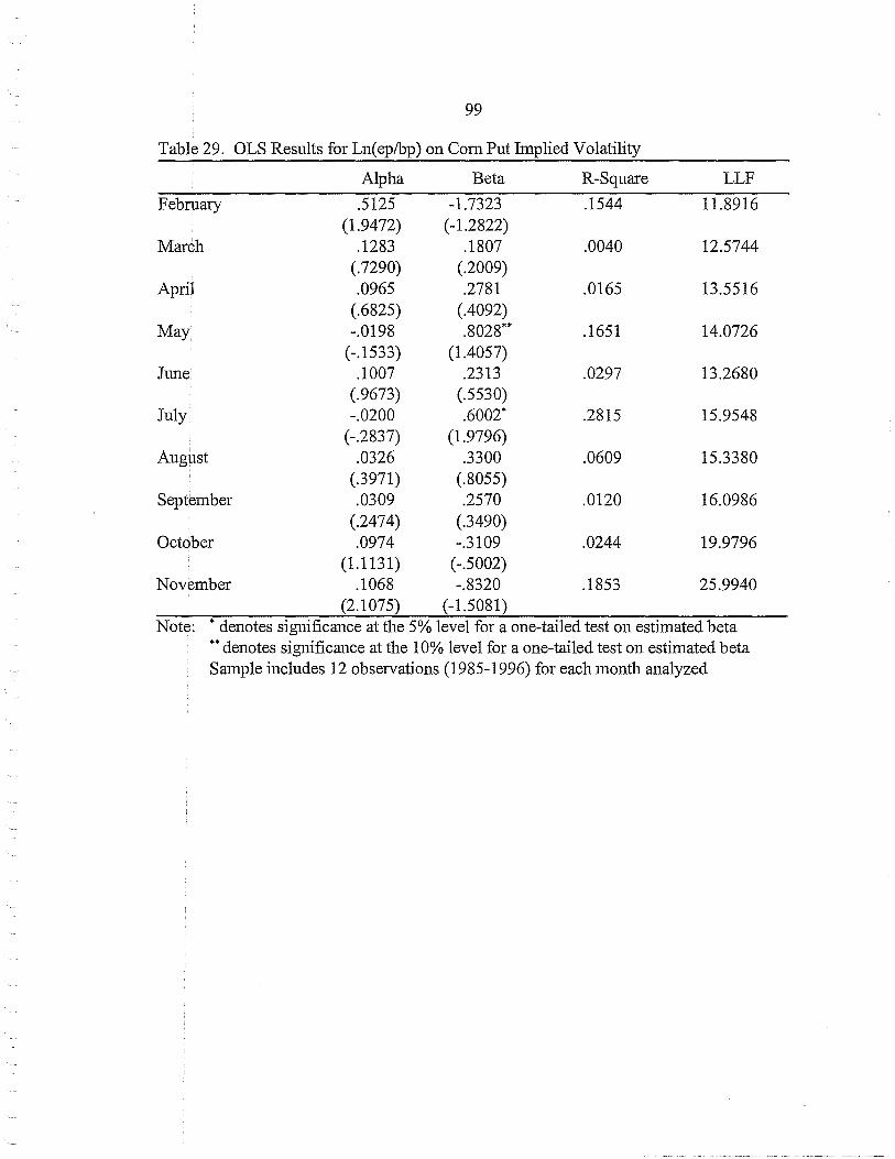
99

Table 29. OLS Results for Ln( ep/bp) on Com Put hnplied Volatility

Alpha Beta R-Square LLF

February .5125 -1.7323 .1544 11.8916 (1.94 72) ( -1.2822)

March .1283 .1807 .0040 12.5744 (.7290) (.2009)

April .0965 .2781 .0165 13.5516 (.6825) (.4092)

May -.0198 .8028** .1651 14.0726 (-.1533) (1.4057)

June .1007 .2313 .0297 13.2680 (.9673) (.5530)

July -.0200 .6002* .2815 15.9548 (-.2837) (1.9796)

August .0326 .3300 .0609 15.3380 (3971) (8055)

September .0309 .2570 .0120 16.0986 (.2474) (.3490)

October .0974 -.3109 .0244 19.9796 (1.1131) (-.5002)

November .1068 -.8320 .1853 25.9940 (2.1075) (-1.5081)

Note: * denotes significance at the 5% level for a one-tailed test on estimated beta **denotes significance at the 10% level for a one-tailed test on estimated beta Sample includes 12 observations (1985-1996) for each month analyzed

100

Table 30. OLS Results for Ln(hp/pp) on Soybean Call Implied Volatility

Alpha Beta R-Square LLF

February .1309 -.0414 .0006 16.0175 (1.5364) ( -.0762)

March .0401 .5258 .0661 17.0284 (.3901) (.8415)

April .0767 .2018 .0134 17.5605 (.8031) (.3687)

May .1903 -.4787 .1069 19.0126 (2.2928) (-1.0939)

June -.0300 .6308* .2926 17.9935 (-.4511) (2.0335)

July -.0117 .4164* .2765 20.7682 ( -.2629) (1.9549)

August .0271 .2261 .0720 19.0731 (.5930) (.8811)

September -.0095 .5605** .1940 20.9419 (-.1939) (1.5513)

October .0257 .2226 .0294 24.5350 (.6817) (.5504)

Note: * indicates significance at the 5% level for a one-tailed test ** indicates significance at the 10% level for a one-tailed test Sample includes 12 observations (1985-1996) for each month analyzed

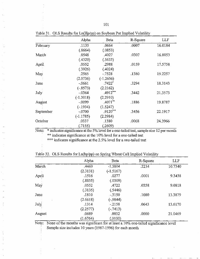
101

Table 31. OLS Results for Ln(Hp/pp) on Soybean Put Implied Volatility

Alpha Beta R-Square LLF

February .1135 .0664 .0007 16.0184 (.8664) (.0853)

March .0548 .4027 .0307 16.8053 (.4329) (.5633)

April .0552 .2988 .0159 17.5758 (.3926) (.4024)

May .2565 -.7528 .1380 19.2257 (2.0736) ( -1.2656)

June -.0661 .7422* .3294 18.3143 (-.8573) (2.2162)

July -.0364 .4912*** .3442 21.3573 (-1.3018) (2.2910)

August -.0099 .4071 ** .1886 19.8787 (-.1934) (1.5247)

September -.0700 .9120*** .3456 22.1917 (-1.1785) (2.2984)

October .0337 .1380 .0068 24.3966 (.7155) (.2609)

Note: * indicates significance at the 5% level for a one-tailed test, sample size 12 per month ** indicates significance at the 10% level for a one-tailed test ***indicates significance at the 2.5% level for a one-tailed test

Table 32. OLS Results for Ln(hp/pp) on Spring Wheat Call Implied Volatility

Alpha Beta R-Square LLF

March .4469 -1.5804 .2234 10.7340 (2.3131) (-1.5167)

April .1516 .0277 .0001 9.3438 (.8855) (.0309)

May .0552 .4722 .0358 9.0818 (.3135) (.5446)

June .1810 -.3150 .1080 13.3879 (2.6618) (-.9844)

July .1314 -.2158 .0643 13.6170 (2.2577) (-.7413)

August .0689 .0032 .0000 21.0469 (1.6764) (.0100)

Note: None ofthe months was significant for at least a 10% one-tailed significance level Sample size includes 10 years (1987-1996) for each month

102

Table 33. OLS Results for Ln(hp/pp) on Spring Wheat Put Implied Volatility

Alpha Beta R-Square LLF

March .2642 -1.2832 .0397 3.1268 (.6399) (-.5747)

April .3000 -1.5074 .0988 3.3057 (.9494) ( -.9363)

May .2515 -1.2974 .0779 3.4085 (.7889) (-.8217)

June -.0771 .3874 .0310 5.9471 ( -.4807) (.5063)

July -.0270 .2531 .0253 8.0266 (-.2443) (.4561)

August -.0112 .2942 .0159 12.4715 (-.1011) (.3592)

Note: None of the months was significant for at least a 10% one-tailed significance level Sample size includes 10 years (1987 -1996) for each month

103

wrong sign (is negative) but is insignificant. For puts, beta for February is negative but

positive for March. Neither are significant.

Results are similar for soybeans. For soybeans calls, June and July have positive and

significant beta estimates and alpha estimates which don't significantly differ from zero.

For soybean puts June, July, August, and September are significant. It is interesting to note

that for both soybean puts and calls, May has a beta estimate which is negative and

significant and an alpha which appears to be significantly different from zero. Again,

February and March are not significant with respect to crop insurance rate setting purposes.

For soybean calls, February has a negative beta which is insignificant and an alpha

significantly different from zero. Otherwise, beta estimates are positive but insignificant.

Results for spring wheat appear to be the poorest ofthe three crops tested. For spring

wheat calls, March has a negative, insignificant beta and an alpha which is significantly

different fi·om zero. For puts, none of the beginning period months have significant beta

estimates. The "best" month, April, has the wrong sign.

Overall it can be concluded that volatilities implied in futures options premia are very

poor predictors of futures price variability. Despite the fact that there are some months in

which beta estimates are significant, there is no evidence to support that implied volatilities

have useful information in predicting futures price variance. It is interesting to note,

however, that the most significant beginning period seems to be around June or July (at least

for com and soybeans), which is around the peak time for implied volatility. Again, this may

be attributed to the fact that early in the year such as in February, little is lmown about the

crop. Hennessy and Wahl point out that as the season progresses, information about the crop

104

becomes increasingly available. It seems plausible that better forecasts of futures price

variance should be made during these "peale" months, which is empirically the case for com

and soybeans.

Heteroskedasticity

The options market is relatively new. Options on futures have actively traded for

only a little more than a decade. For com and soybeans, we have Chicago Board of Trade

(CBOT) data beginning in 1985, thus giving us only 12 years of data. For spring wheat, we

have data beginning in 1987 which is 10 years of data.

One interesting question that arises is whether the option market has improved over

time. fu other words, do option prices today better convey information than those from, say,

1986 when the market was young?

To test whether the options market has become more efficient, a heteroskedastic

model is estimated. Heteroskedasticity occurs when the error variance is non-constant.

When considering whether the options market has become more efficient over time, testing

for heteroskedasticity is important since error variance should decrease if the markets are

truly becoming more efficient over time.

A multiplicative heteroskedastic model is used. This model has the empirical form:

(Z a) var = e 1

Such a model specifies the variance var as a function of exogenous parameters Z1 and a

vector of unlmown parameters a. fu this model, Z represents a "learning" index for market

105

age, ranging from Z=1 in 1985 to Z=12 in 1996. Such a variable seems appropriate if we are

testing whether the options market is improving over time. As such, this variable is defined

as time in the data set.

The heteroskedastic model thus estimates an equation of the form

var = CX0

+ cx1 (Time)

where h is the variance, time is the exogenous variable Z which is hypothesized to affect the

variance, and ai are the parameters estimated in the variance equation. 32

The parameter of interest is a1• If a1 is negative, then the error variance is decreasing

over time, which means the market is becoming "better." If a1 is positive then it is unlikely

that the market is improving. If a1 is zero then there is no effect on the market's "efficiency"

overtime.

A way to test for heteroskedasticity (denoted hereafter as HE I) is to compute the log

of the likelihood functions obtained from the OLS and HET models. If the two statistics do

not differ significantly, then OLS cannot be rejected. If there is significant difference, then

heteroskedasticity is more likely.

In this empirical framework, OLS is considered a restricted model, since it essentially

assuines or "restricts" the error variance to be constant. HET is considered the unrestricted

model, since error variance is allowed to change.

32The heteroskedastic model is estimated using Shazam, and for models with exogenous heteroskedasticity Shazam estimates an intercept term in the variance equation.

106

The appropriate test to consider is discussed in Judge, et al.. The test statistic of

interest is given by:

LR = 2[LLF(HET) - LLF(OLS)] - X2 (2)

LLF(HET) is the log likelihood function of the HET (unrestricted) model, while LLF(OLS)

is from the OLS (restricted) model33• It can be shown that this statistic is distributed as a X2

with degrees of freedom k equal to the number of restrictions. In this case there is one

restriction; thus there is only one degree of freedom. OLS is rejected if the test statistic LR

is too large, that is, if it exceeds the appropriate chi-squared statistic.

Results for heteroskedasticity are summarized in tables 34 through 36. Each table

summarizes results for the HET model from both puts and calls. Shown is the LR for calls,

the LR for puts, and the estimated coefficient on time. T -statistics are shown in parentheses.

If there is indeed heteroskedasticity in which the error variance is decreasing over time as a

result of"learning" in the market, then it is expected that coefficient estimates on time would

be negative and significantly different from zero.

For com, OLS is rejected in August for both calls and puts based on the LR test at

a significance level of alpha=.025. When considering the coefficients on time, however, beta

is positive and significant, which is not the sign expected if error variance is decreasing over

time.

33It is actually the absolute value of the LR statistic which is of interest. If LLF(OLS) were greater than LLF(HET) then it would be necessary to multiply by -2 instead of2.

107

Table 34. Heteroskedasticity for Corn, Ln( eplbp) on Implied Volatility

LR (Calls) Time LR (Puts) Time

February .8650 -.1349 ******** ******** (-1.0000) ******** ********

March 1.7078 -.1779 1.4828 -.1618 (-1.5040) (-1.3680)

April 1.0376 -.1426 1.1104 -.1453 (-4.2426) (-1.2290)

May .8330 -.1532 .9498 -.1582 (-1.2960) (-1.3370)

June .3750 -.1107 .3952 -.1173 (-.9364) (-.9918)

July .4480 .0962 .5584 .1048 (.8137) (.8859)

August 5.9680* .3380 5.9034* .3393 (2.8580) (2.8690)

September 2.2156 .2122 2.3564 .2458 (1.794) (2.0780)

October .0034 .0087 .0255 .0243 (.0740) (.2056)

November 1.1602 .2558 1.4308 -.1622 (2.1630) (-1.3720)

Note: Asymptotic t-values shown in parentheses LR statistic is distributed X2

<1l

*denotes OLS rejected based on LR test at alpha=.025 significance Sample size includes 12 years of data for each month

108

Table 35. Heteroskedasticity Results for Soybeans, Ln(hp/pp) on Implied Volatility

LR (Calls) Time LR (Puts) Time

February .2998 -.0653 .2232 -.0527 ( -.5523) ( -.4453)

March .2278 -.0524 .3722 -.0698 ( -.4434) ( -.5900)

April 9.6886* -.5968 7.5276** -.4062 (-5.046) (-3.4350)

May 7.5438** -.5174 5.5172*** -.4573 (-4.3750) (-3.8670)

Jm1e 1.1148 -.1142 2.8772**** -.1859 (-.9652) (-1.5720)

July .7052 -.1348 2.2252 -.2320 (-1.1390) (-1.9620)

August .1142 .0557 .0428 .0313 (.4706) (.2650)

September .0678 .0399 .1562 -.0677 (.3372) (-.5725)

October 1.4426 .2343 2.7126**** .4377 (1.9810) (3.7010)

Note: Asymptotic t-values shown in parentheses LR statistic is distributed X2

ct)

Sample size includes 12 years of data for each month *denotes OLS rejected based on LR test at alpha=.005 significance **denotes OLS rejected based on LR test at alpha=.010 significance ***denotes OLS rejected based on LR test at alpha =.025 significance ****denotes OLS rejected based on LR test at alpha=.100 significance

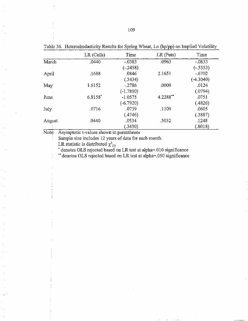
109

Table 36. Heteroskedasticity Results for Spring Wheat, Ln (hp/pp) on Implied Volatility

LR (Calls) Time LR (Puts) Time

March .0440 -.0383 .0963 -.0833 (-.2458) ( -.5353)

April .1688 .0846 2.1651 -.6702 (.5434) (-4.3040)

May 1.6152 -.2786 .0009 .0124 (-1.7890) (.0794)

June 6.8158* -1.0575 4.2288** .0751 (-6.7920) (.4826)

July .0716 .0739 .1109 .0605 (.4746) (.3887)

August .0440 .0534 .5052 .1248 (.3430) (.8018)

Note: Asymptotic t-values shown in parantheses Sample size includes 12 years of data for each month LR statistic is distributed X2c1)

*denotes OLS rejected based on LR test at alpha=.010 significance **denotes OLS rejected based on LR test at alpha=.050 significance

110

For soybeans, April is rejected for calls based on the LR test at alpha=.005.

Furthermore, the estimated coefficient on time is negative and significant. For April puts and

May calls OLS is rejected at alpha=.Ol, for May puts at alpha=.025, and for June and

October puts at alpha=.lOO. For October puts, however, the coefficient on time has the

wrong (positive) sign.

For spring wheat, June calls are rejected based on the LR test at alpha=.OlO.

Furthermore, the coefficient on time is negative and significant. June puts are rejected at

alpha=.050, but time has the wrong sign.

Overall, the hypothesis that the futures options market is becoming better over time

is not strongly supported. There are a few instances in which heteroskedasticity looks

probable, such as in August for com, April and May for soybeans, and June for spring wheat.

When further considering the estimated coefficients on time, however, the likelihood of

heteroskedasticity is narrowed down to April and May for soybeans and June for spring

wheat, since it is expected that the coefficient on time would be negative if options markets

were indeed improving over time.

Furthermore, with respect to crop insurance, there seems to be no improvement in

Febmary or March for the futures options market. Since Febmary and March is around the

sign up period, testing for heteroskedasticity seems most relevant in these months.

Overall, there is not much validity in the "learning" story for com, soybean, and

spring wheat futures options.

111

CONCLUSIONS

Summary ofResults

This thesis tests important Black-Scholes distributional assumptions and also the

infmmational content of com, soybean, and spring wheat futures options prices as potential

predictors of futures price changes. Data used included com, soybean, and spring wheat

futures price data from 1960 through 1996, com and soybean futures options data from 1985

through 1996, and spring wheat futures options data from 1987 through 1996

There are several findings regarding assumptions maintained by the original Black­

Scholes option pricing formulas (1973) and the subsequent extension to futures options

prices by Black (1976). Black-Scholes assumes that futures prices are lognormally

distributed with a constant variance rate parameter (implied volatility), and that current

futures prices are unbiased estimates for later futures prices.

First, it is found that standard deviations of the natural logarithm of daily price

changes calculated within months display seasonality across months. These historical

standard deviations are low early in the year, rise and peak during mid-year (summer)

months, and fall as the appropriate contract maturity month (December, November, and

September for com, soybeans, and spring wheat) approaches. This is consistent with futures

price seasonality findings already in the literature. This seasonality contradicts Black-

112

Scholes constant volatility assumptions. One point that is stressed throughout this thesis is

that tests ofBlack-Scholes assumptions are in actuality simultaneous tests ofBlack-Scholes

model and the efficiency of the futures option market.

A second conclusion is that average futures prices for successive beginning periods

starting with February are indeed unbiased estimates for ending period futures prices.

A third important finding which primarily concerns the Black-Scholes analysis and

the Black formula is that the assumption of lognormality is widely rejected for com,

soybeans, and spring wheat futures prices. Lognormality is the most important distributional

assumption maintained by the Black formula; rejection oflognormality is evidence which

casts doubt on the validity ofBlack-Scholes distributional assumptions. It is also found that

excess kurtosis is the main reason why lognormality is often rejected.

A fourth finding is that implied volatilities calculated from the Black formula display

seasonal patterns. This seasonality is further evidence that Black-Scholes assumptions are

inaccurate, since Black-Scholes assumes that the implied volatility parameter is constant.

Although there is seasonality in implied volatility, we find that implied standard

deviation is fairly well behaved, i.e. decreasing over the course of a year. Although there are

instances in which implied standard deviation peaks in mid-year, there is no significant

evidence to support the notion that there is seasonality in these measures also. Overall, the

futures options market appears to be "correcting" the seasonality in implied volatility.

A second set of results concerns the potential usefulness of agricultural futures

options in predicting the variance in futures prices. Despite the fact that most Black-Scholes

assumptions are statistically rejected, it is still hypothesized that implied volatilities may be

113

useful in predicting the variability of futures prices. Mayhew points out that implied

volatility may still be considered an optimal assessment of futures variability, and even if

futures price volatility is lmown to be stochastic implied volatility may be interpreted as the

market's average assessment of variability over the remaining life of the option.

First, an OLS regression of the absolute value of the natural logarithm of the ratio

of beginning period to ending period futures prices on implied volatility was estimated.

Overall, these implied volatilities are poor predictors of subsequent realized price changes

for individual successive beginning periods starting with February and moved forward until

one month prior to contract maturity.

As a possible explanation for the poor results of the "informational content" tests for

corn, soybean, and spring wheat puts and calls, a heteroskedastic model is estimated, where

error variance is hypothesized to be a function of market age (time). We are interested in

whether the agricultural futures options market has improved over time, as these futures

options have only traded for slightly more than a decade. Overall, heteroskedasticity is not

significant for any of these three crops. There is no evidence to suggest that there has been

"learning" or improved efficiency in these markets over time.

Implications

The empirical results in this thesis suggest the direction for future research, in order

to evaluate the use of futures options prices to recover ex-ante probabilistic information

about second and higher moments of futures price distributions. As discussed, applications

of the general Cox and Ross (197 6) option pricing formula (equation 5) may be used, and

114

various distributions have been proposed as alternatives to the commonly used lognormal.

Many of these alternate distributions have the advantage of providing more flexible

parameterization than the lognormal. The lognormal is inflexible in that it does not allow

for varying degrees of skewness and kurtosis, which may be better handled by other, more

flexible distributions.

Sherrick, Irwin and Foster (1996) discuss the use of the BURR-XII distribution,

which they point out has become a popular distribution for modeling prices and which has

been utilized extensively by the insurance industry. Empirically, Sherrick, et. al. find that

the BURR-XII generally performs better than the lognormal. Faclder and King also discuss

the use of the BURR-XII (parametric) distribution as well as non-parametric methods.

Sherrick, Garcia, and Tirupattur (1996) propose the use ofthe BURR-ill distribution,

another "flexible" distributional candidate. They find that in depicting ex-ante price

variability, the BURR-ill substantially outperforms the lognormal.

Myers and Hanson (1993) suggest the use of a generalized autoregressive conditional

heteroskedastic (GARCH) process. They recognize that the lognormal may be an

inappropriate representation of futures price changes and also that volatility may be

stochastic, thereby suggesting the use of the GARCH model. Myers and Hanson also point

out that the GARCH model does a good job of modeling excess kurtosis and time-varying

volatility, which are shown in this thesis to be two possible problems with the use of the

Black-Scholes model and the assumption of lognormality. When testing a GARCH

specification for CBOT soybean futures prices, Myers and Hanson find that the model

115

estimates actual market prices significantly better than the Black formula, which further

supports the need for more flexible distributional models.

A key point in this discussion concerns seasonality. Overall, it is found that historical

futures price standard deviation and implied volatility display strong, systematic seasonal

patterns. Neither the GARCH models nor the BURR distributions incorporate variables

which account for such systematic seasonality; thus, seasonality presents serious challenges

to the proposed models. ·

116

LITERATURE CITED

Beckers, Stan. "Standard Deviations Implied in Option Prices as Predictors of Future Stock Price Variability." Journal ofBanking and Finance 5 (1981).

Black, Fischer and Myron Scholes. "The Pricing of Options and Corporate Liabilities." Journal ofPolitical Economy. May-June 1973.

Black, Fischer. "The Pricing of Commodity Contracts." Journal of Financial Economics. March, 1976.

Campbell, John Y., Andrew W. Lo and A. Craig MacKinlay. The Econometrics of Financial Markets. Princeton University Press. Princeton, NJ. 1997

Canina, Linda and Stephen Figlewski. "The Informational Content of Implied Volatility." The Review ofFinancial Studies. 1993. Volume 6. Number 3.

Chiras, Donald and Steven Manaster. "The Information Content of Option Prices and a Test ofMarket Efficiency." Journal ofFinancial Economics. 6 (1978).

Cox, John C. and Stephen A. Ross. "Some New Results in Financial Option Pricing Theory." Journal ofFinance. Volume XXXI. No.2. May, 1976.

Faclder, Paul and Robert P. King "The Evaluation ofProbability Distributions with Special Emphasis on Price Distributions Derived from Option Premiums." Proceedings of a Seminar Sponsored by Southern Regional Project s-180. August, 1987

Forhme, Peter. "Anomalies in Option Pricing: The Black-Scholes Model Revisited." New England Economic Review. March/April1996.

Gardner, Bruce L. "Commodity Options for Agriculture." American Journal of Agricultural Economics. December, 1977.

Heifner, Richard. "Price Analysis for Determining Revenue Insurance Indemnities and Premiums." Report to Office ofRisk Management. September, 1996.

117

Hennessy, David and Thomas I. Wahl. "The Effects ofDecision Making on Futures Price Volatility." American Journal of Agricultural Economics. 78. August, 1996.

Hieronymus, Thomas A. The Economics of Futures Trading. Commodity Research Bureau, Inc. New York, NY, 1971.

Hull, John C. Options, Futures, and Other Derivative Securities. Prentice Hall. Upper Saddle River, NJ. 3rd Edition. 1997.

Judge, George C., R. Carter Hill, William E. Griffiths, Helmut Lutkepohl, and Troung­Chao Lee. Introduction to the Theozy and Practice of Econometrics. 2nd Edition. John Wiley and Sons, Inc. New York, 1988.

Mayhew, Stewart. "Implied Volatility." Financial Analysts Journal. July-August, 1995.

Merton, Robert C. "Theory of Rational Option Pricing." Bell Journal of Economics and Management Science. 4. Spring 1973.

Myers, Robert J. and Steven D. Hanson. "Pricing Commodity Options When the Underlying Futures Price Exhibits Time-Varying Volatility." American Journal of Agricultural Economics. 75. February 1993.

Sherrick, Bruce, Philip Garcia, and Viswanath Tirupattur. "Recovering Probabilistic Information from Options Markets: Tests ofDistributional Assumptions." Journal ofFutures Markets. Vol. 16, No.5. 1996.

118

APPENDIX

119

Table 37: Sample Size for Com Call Futures Options Implied Volatilities

Feb Mar Apr May Jun Jul Aug Sep Oct Nov 1985 2 18 18 21 18 20 22 19 22 6 1986 18 20 15 19 18 21 20 21 23 5 1987 16 22 21 20 22 22 20 21 22 15 1988 19 21 20 21 22 20 23 21 21 14 1989 17 22 19 21 21 20 23 20 22 13 1990 19 22 20 22 21 21 23 19 23 16 1991 17 20 20 21 18 22 22 20 23 11 1992 18 22 17 19 22 22 21 21 22 15 1993 14 20 20 19 21 21 22 21 21 15 1994 18 21 19 21 22 20 23 21 21 14 1995 19 23 19 22 22 20 23 20 22 13 1996 20 21 21 22 20 22 22 20 23 11

Table 38: Sample Size for Com Put Futures Options Implied Volatilities

Feb Mar Apr May Jun Jul Aug Sep Oct Nov 1985 2 14 19 21 20 22 22 20 23 6 1986 19 20 22 21 21 22 21 21 23 5 1987 18 17 20 19 19 22 21 21 22 15 1988 12 12 18 19 19 20 23 20 21 14 1989 14 19 19 22 21 20 23 20 22 13 1990 19 20 20 19 20 21 23 19 23 16 1991 10 19 19 22 10 22 22 20 23 11 1992 10 17 17 19 19 22 21 21 22 15 1993 8 13 21 20 22 21 22 21 22 15 1994 15 20 19 21 22 20 23 21 21 14 1995 19 22 19 22 22 20 23 20 20 13 1996 19 21 20 21 20 22 22 20 23 11

120

Table 39: Sample Size for Soybean Call Futures Options Implied Volatilities

Feb Mar Apr May Jun Jul Aug Sep Oct 1985 14 18 19 21 20 22 22 20 9 1986 15 19 21 21 18 20 18 19 8 19.87 16 20 21 20 22 22 21 21 17 1988 19 23 20 21 22 20 23 21 15 1989 17 17 20 21 21 19 22 20 15 1990 19 22 20 22 21 21 23 19 15 1991 14 18 14 17 14 21 22 20 13 1992 16 20 17 20 22 22 21 21 17 1993 18 18 21 20 22 21 22 21 15 1994 18 23 18 21 22 20 23 21 15 1995 19 23 19 22 22 20 23 20 15 1996 20 21 21 22 20 22 22 20 14

Table 40: Sample Size for Soybean Put Futures Options Implied Volatilities

Feb Mar Apr May Jun Jul Aug Sep Oct 1985 13 19 13 22 19 22 22 20 9 1986 10 16 16 19 18 20 21 21 13 1987 17 15 18 18 20 22 21 21 17 1988 9 13 14 18 22 20 23 19 15 1989 9 16 18 19 22 20 23 20 15 1990 15 18 17 22 21 21 23 19 15 1991 6 8 14 22 20 21 22 20 14 1992 12 14 14 17 19 22 21 21 17 1993 15 13 12 12 21 19 22 21 16 1994 12 15 16 19 20 20 23 21 15 1995 14 12 15 22 18 16 23 20 15 1996 17 17 19 22 19 21 22 19 14

121

Table 41: Sample Size for Spr. Wheat Call Futures Options Implied Volatilities

I '-~

Feb Mar Apr May Jun Jul Aug 1987 3 13 15 19 16 11 13

I 1988 5 6 11 19 22 20 15

- 1989 10 18 17 22 19 20 13 1990 7 5 8 14 17 17 18 1991 3 11 19 18 18 20 17 1992 12 17 16 15 22 22 9 1993 4 13 19 20 21 21 15 1994 2 17 17 21 21 20 15 1995 9 18 19 22 22 20 14 1996 11 18 21 22 19 21 17

' ,_

Table 42: Sample Size for Spr. Wheat Put Futures Options for Implied Volatilities

Feb Mar Apr May Jun Jul Aug 1987 2 12 11 12 18 22 13 1988 2 3 3 16 19 17 15 1989 4 11 7 14 17 19 14 1990 3 7 9 17 20 20 12 1991 2 6 11 18 20 22 15 1992 11 12 13 16 21 22 15 1993 5 20 19 20 22 21 14 1994 13 8 15 18 17 19 14 1995 0 14 18 16 13 20 14 1996 8 8 15 16 19 22 17