Embed Size (px)
Citation preview

Manus
cript
Tetrahedral vs. polyhedral mesh size evaluation on flow velocity and wall shear stress forcerebral hemodynamic simulation
Martin Spiegela,b,c,d*, Thomas Redelc, Y. Jonathan Zhange, Tobias Struffertb, Joachim Horneggera,d, Robert G. Grossmane,
Arnd Doerflerb and Christof Karmonike
aPattern Recognition Lab, Department of Computer Science, Friedrich-Alexander University Erlangen-Nuremberg (FAU), Erlangen,Germany; bDepartment of Neuroradiology, FAU, Erlangen, Germany; cSiemens AG Healthcare Sector, Forchheim, Germany; dErlangenGraduate School in Advanced Optical Technologies (SAOT), Erlangen, Germany; eThe Methodist Hospital Research Institute, Houston,
TX, USA
(Received 11 May 2010; final version received 23 August 2010)
Haemodynamic factors, in particular wall shear stresses (WSSs) may have significant impact on growth and rupture of cerebralaneurysms. Without a means to measure WSS reliably in vivo, computational fluid dynamic (CFD) simulations are frequentlyemployed to visualise and quantify blood flow from patient-specific computational models. With increasing interest inintegrating these CFD simulations into pretreatment planning, a better understanding of the validity of the calculations inrespect to computation parameters such as volumeelement type,mesh size andmesh composition is needed. In this study, CFDresults for the two most common aneurysm types (saccular and terminal) are compared for polyhedral- vs. tetrahedral-basedmeshes and discussed regarding future clinical applications. For this purpose, a set of models were constructed for eachaneurysmwith spatially varying surface and volumemesh configurations (mesh size range: 5119–258, 481 volume elements).WSSdistribution on themodelwall and point-based velocitymeasurementswere compared for each configurationmodel. Ourresults indicate a benefit of polyhedral meshes in respect to convergence speed and more homogeneous WSS patterns.Computational variations of WSS values and blood velocities are between 0.84 and 6.3% from the most simple mesh(tetrahedral elements only) and the most advanced mesh design investigated (polyhedral mesh with boundary layer).
Keywords: mesh size evaluation; mesh independence analysis; polyhedral; tetrahedral; wall shear stress; blood flowvelocity
1. Introduction
Ischaemic stroke, being the third common cause of death in
the western world, is a serious clinical event. Of the two main
causes of a stroke, arterial obstruction and intra-cerebral
haemorrhage, about 10–15% of the latter are induced by the
rupture of a cerebral aneurysm (Winn et al. 2002). More and
more cerebral aneurysms are now incidentally detected
because of recent advances in the field of medical imaging
techniques such as 64 slice computation time (CT) or
magnetic resonance imaging (MRI) at 3T. So far, the reason
for growth or rupture of an aneurysm is not entirely
understood, but it is assumed that the haemodynamic within
an aneurysm plays an important role (Jou et al. 2008).
Geometric factors, e.g. lesion size and aspect ratio (AR)
(Ujiie et al. 2001; Nader-Sepahi et al. 2004; Raghavan et al.
2005) are also considered to determine the risk of rupture.
However, even haemodynamic information together with
geometric aspects has so far proven insufficient for the
calculations of a reliable patient-specific risk index for a
particular aneurysm. Other biological mechanisms and
systemic conditions may also contribute to aneurysm
rupture. To assess intra-aneurysmal haemodynamics,
computational fluid dynamic (CFD) simulations have been
employed with patient-specific geometries derived from
clinical image data in Steinman et al. (2003), Hoi et al.
(2004), Karmonik et al. (2004), Shojima et al. (2004), Cebral
and Lohner (2005), Cebral et al. (2005b) and Venugopal et al.
(2007). A reliable patient-specific CFD-based blood flow
simulation will be strongly influenced by two factors: (1) the
geometric accuracy of the patient-specific vascular model
dependent on the segmentation method used and (2) the
boundary conditions and simulation parameters such as
inflow blood speed, blood density/viscosity and rigid
walls. Patient-specific boundary conditions can either be
obtained through invasive measurements during treatment
(i.e. pressure catheter) or, as demonstrated recently, by 2-D
phase-contrast MRI providing the time-varying blood flow
profile at the inlet of the computational model as shown in
Karmonik et al. (2008). The sensitivity of other compu-
tational parameters on the simulation results, in particular
mesh size and mesh design, has not been evaluated in detail
for this particular vascular pathology. The haemodynamic
situation in cerebral aneurysms is favourable to be simulated
ISSN 1025-5842 print/ISSN 1476-8259 online
q 2010 Taylor & Francis
DOI: 10.1080/10255842.2010.518565
http://www.informaworld.com
*Corresponding author. Email: [email protected]
Computer Methods in Biomechanics and Biomedical Engineering
iFirst article, 2010, 1–14
Downloaded By: [informa internal users] At: 15:06 4 January 2011

Manus
cript
using CFD: blood flow in cerebral vessels is always
antegrade as compared to the blood flow in the aorta with
modest pulsatility. Unless downstream vascular disease is
present such as a stenotic lesion distal to the aneurysm,
vascular resistance is low. Reynolds numbers are low (in the
order of 100 s) and, therefore, no turbulence flow can be
expected. Due to these favourable conditions, most studies so
far have successfully employed simple meshes such as
tetrahedral meshes with no adaptation or boundary layer.
Still, the assessment of the mesh quality is considered as a
very important task, because inaccurate meshing including
high skewness (SN) of cells or course spatial resolution may
lead to non-valid CFD results and thus leading to potentially
inaccurate local velocities or wall shear stress (WSS)
patterns. In particular, for a future clinical CFD-based
diagnostic and treatment tool, the performed simulations
have to be fast and stable. The mesh size has to be as small as
possible, but concerning accuracy as fine as necessary to
avoid numerical prediction errors (velocity and WSS). Two
different approaches are known to verify the mesh suitability
for CFD simulation introduced by Prakash and Ethier
(2001): (1) Comparison of CFD results with experimental
measured data and (2) a mesh independence analysis. This
work applies the second approach to evaluate the impact of
varying surface and volume mesh resolutions as well as
different meshing techniques represented by polyhedral
(Oaks and Paoletti 2000) and tetrahedral meshes. In
particular, the question which mesh granularity can be
considered as accurate enough to get reliable blood flow
simulation results is investigated with time restraints existing
for future clinical applications in mind. A preliminary
version of this work was reported by Spiegel et al. (2009).
Two cerebral vessel geometries were investigated, i.e. a
sidewall aneurysm of the internal carotid artery and a basilar
bifurcation aneurysm as depicted in Figure 1. Blood flow
velocity and WSS distributions according to varying spatial
mesh resolutions and configurations (polyhedral vs. tetra-
hedral elements) are evaluated. Effects of boundary layer
regarding WSS are studied by means of comparing boundary
layer-based meshes with those exhibiting no boundary layer.
Unsteady simulations are performed with varying time step
(TS) to determine the largest step delivering still valid
simulation results.
2. Methods
3-D digital subtraction angiography image data (Heran et al.
2006) of the two cerebral aneurysms (see Figure 1) were
acquired during endovascular interventions using Siemens
C-arm System (AXIOM Artis dBA, Siemens AG Healthcare
Sector) in Forchheim (Germany) and Houston, TX (USA).
3-D image reconstructions of both aneurysms led to an
image volume for case 1 of 138.24 £ 138.24 £ 57.72 mm
with a voxel spacing of 0.27 £ 0.27 £ 0.13 mm and for
case 2 97.28 £ 97.26 £ 66.43 mm (voxel spacing 0.19 £
0.19 £ 0.1 mm), respectively. The non-isotropic voxel
spacing comes from image downsampling in x/y-direction
due to segmentation and memory issues. For mesh
generation and smoothing, the marching cubes (Lorensen
andCline 1987) and a Laplacian-based smoothing algorithm
(VTKKitware Inc., Clifton Park, NY, USA) were applied as
an additional step. The image data were stored as a
stereolithographic file providing the input data for the
meshing software GAMBIT (ANSYS Inc., Canonsburg, PA,
USA) The mesh corresponding to case 1 exhibits a volume
of 537mm3 and the mesh of case 2 of 282mm3. The
maximal diameters of the inlet and outlets are as follows: (1)
case 1: inlet 5.2mm, outlet 1 2.0mm, outlet 2 2.3mm and
outlet 3 2.6mmand (2) case 2: inlet 3.3mm, outlet 1 2.5mm,
outlet 2 1.5mm, outlet 3 1.5mm and outlet 4 2.4mm.
Different surface mesh resolutions were generated by
using the GAMBIT curvature size function (Cooperation
2007). This function constraints the angle between
outward-pointing normals for any two adjacent surface
triangles. That leads to a denser mesh resolution in areas
exhibiting high curvature like the aneurysm and coarser
resolution in more flat regions. Four parameters define the
curvature size function, i.e. angle, growth, max. and min.
triangle size. Table 1 contains a detailed overview of the
applied curvature size function parameters as well as the set
of meshes. The final number of triangles representing the
surface mesh is automatically determined by the meshing
algorithm according to the chosen parameter values and the
geometry. The resolution of the surface mesh rules the final
number of tetrahedral control volume elements – the larger
the number of surface triangles, the larger is the number of
tetrahedral control volume elements.
To study the effects of boundary layer usage, almost all
meshes (see Table 1) were generated without and with
Figure 1. 3-D mesh representations of the evaluated aneurysms:(a) case 1 depicts an internal carotid aneurysm and (b) case 2illustrates a basilar tip aneurysm. The red spheres show thepositions of the velocity measurement points distributed in thevicinity of the aneurysms, i.e. at the inlet, within the aneurysmand at the outlet.
M. Spiegel et al.2
Downloaded By: [informa internal users] At: 15:06 4 January 2011

Manus
cript
Tab
le1
.S
eto
fm
esh
es–
case
1an
dca
se2
.
#T
et.
cell
s(B
L)
Dif
fere
nce
no
-B
Lto
BL
for
Tet
.ce
lls
in(%
)#
Po
ly.
cell
s(B
L)
Dif
fere
nce
no
-BL
toB
Lfo
rP
oly
.ce
lls
in(%
)
Dif
fere
nce
Po
ly.
vs.
Tet
.in
(%)
Dif
fere
nce
Po
ly.
vs.
Tet
.B
Lin
(%)
Dif
fere
nce
Po
ly.
BL
vs.
Tet
.n
on
-B
Lin
(%)
Max
./m
in.
tria
ng
leG
row
thA
ng
le
Cas
e1
13
,84
1(2
)–
51
19
(2)
––
––
6/0
.00
11
.22
52
6,7
02
(40
,69
9)
52
.47
28
3(2
4,2
06
)2
32
.42
72
.72
40
.52
9.3
3.6
/0.0
01
1.2
14
52
,37
4(7
7,2
52
)4
7.5
12
,46
7(3
1,5
48
)1
53
.12
76
.22
59
.22
39
.81
.8/0
.00
11
.11
47
6,4
93
(10
9,6
38
)4
3.3
17
,69
5(3
8,5
64
)1
17
.92
76
.92
64
.82
49
.61
.2/0
.00
11
.26
86
,62
1(1
07
,33
6)
23
.91
8,6
81
(32
,01
2)
71
.42
78
.42
70
.22
63
.00
.4/0
.00
11
.11
21
06
,01
0(1
24
,04
1)
17
.02
2,2
97
(35
,86
6)
60
.92
79
.02
71
.12
66
.20
.36
/0.0
01
1.1
12
11
5,0
14
(16
0,7
71
)3
9.8
25
,54
0(4
8,6
87
)9
0.6
27
7.8
26
9.7
25
7.7
0.3
/0.0
01
1.1
10
18
9,6
25
(20
2,5
65
)6
.83
7,4
95
(53
,79
4)
43
.52
80
.22
73
.42
71
.60
.28
/0.0
01
1.1
10
19
7,0
98
(22
8,0
97
)1
5.7
38
,99
1(5
8,8
79
)5
1.0
28
0.2
27
4.2
27
0.1
0.2
7/0
.00
11
.11
02
31
,35
4(2
58
,48
1)
11
.74
5,1
58
(65
,70
7)
45
.52
80
.52
74
.62
71
.60
.25
8/0
.00
11
.11
0
Cas
e2
31
,69
6(4
7,3
11
)4
9.3
88
14
(26
,01
4)
19
5.1
27
2.2
24
5.0
21
7.9
0.4
2/0
.00
11
.21
74
3,0
63
(59
,91
4)
39
.11
0,8
43
(21
,15
3)
95
.12
74
.82
64
.72
50
.90
.37
/0.0
01
1.1
71
75
6,1
76
(75
,44
7)
34
.31
3,2
80
(24
,97
8)
88
.12
76
.42
66
.92
55
.50
.34
/0.0
01
1.1
21
57
5,4
69
(10
0,5
87
)3
3.3
16
,79
5(3
0,4
35
)8
1.2
27
7.7
26
9.7
25
9.7
0.3
2/0
.00
11
.10
13
98
,39
9(1
29
,51
6)
31
.62
1,1
08
(37
,22
1)
76
.32
78
.62
71
.32
62
.20
.3/0
.00
11
.10
10
11
4,2
27
(14
2,3
36
)2
4.6
23
,84
6(3
9,8
33
)6
7.0
27
9.1
27
2.0
26
5.1
0.2
8/0
.00
11
.10
10
14
8,6
25
(15
9,7
97
)7
.53
0,1
67
(44
,65
2)
48
.02
79
.72
72
.12
70
.00
.25
/0.0
01
1.0
98
18
4,2
26
(21
9,9
22
)1
9.4
36
,84
5(6
5,3
98
)7
7.5
28
0.0
27
0.3
26
4.5
0.2
4/0
.00
11
.10
6
Av
g.
29
.29
3.8
27
7.7
26
6.5
25
5.6
Tet
.an
dP
oly
.,te
trah
edra
lan
dpoly
hed
ral,
resp
ecti
vel
yan
dB
L,
boundar
yla
yer
.
Computer Methods in Biomechanics and Biomedical Engineering 3
Downloaded By: [informa internal users] At: 15:06 4 January 2011

Manus
cript
boundary layers (Garimella and Shephard 2000; Loehner
and Cebral 2000). Since a boundary layer approximates the
boundary of the vessel tubes with prisms as shown in
Figure 2, this automatically results in a higher number of
tetrahedral control elements as compared to meshes
without a boundary layer. The boundary layers were
created through GAMBIT’s boundary layer algorithm
featuring two levels. The height of the first level was
chosen to be 0.04 mm and the second one 20% larger, i.e.
0.048 mm. The mesh quality in terms of AR and
surface/mesh SN is summarised in Table 2.
The tetrahedral meshes were imported into the
simulation software Fluent (ANSYS Inc.) A conversion
algorithm, part of the Fluent CFD solver, was used to
generate for each tetrahedral mesh a corresponding
polyhedral mesh. The surface of the vessel models was
assumed to be rigid walls and no slip as shear condition.
Blood was modelled as an incompressible Newtonian fluid
with a density of 1050 kg/m3 and a viscosity of 0.004 N/m2
(Hassan et al. 2004). The boundary conditions for all
conducted simulations were as follows: the inlet was
considered as velocity inlet and all outlets were modelled
as pressure outlet zero. A constant inflow rate of 0.3 and
0.5 m/s was applied in the steady simulations for the case 1
and case 2, respectively. In unsteady simulations, two
different inflow waveforms were used (Figure 3): for case
1, an MRI-measured waveform and for case 2, we applied
a waveform taken from a former publication (Groden et al.
2001) which was measured with ultrasound, since there
was no patient-specific blood flow profile measured with
MRI or ultrasound. Similar blood flow velocity profiles
concerning the basilar artery were also measured by Kato
et al. (2002). Steady-state simulations were considered as
converged if the relative residuals fall under 0.001 (i.e. the
absolute values of the residuals were reduced by 3 orders
of magnitude). In addition, the mass flow was measured to
prove convergence by subtracting outflow from inflow. All
converged solutions exhibit a mass flow difference
between inflow and outflow of ^5 e28.
Seven points were defined to measure the simulated
blood flow velocity occurring in the environment of the
aneurysm. In case 1, two points were placed in the inlet
region of the aneurysm, three inside the aneurysm dome
and two in the outlet region of the aneurysm. In case 2, one
point was located within the inlet vessel part, another one
Figure 2. Meshing example regarding case 2. (a) and (c) showtetrahedral and polyhedral meshes. (b) and (d) depict tetrahedraland polyhedral-based meshes with a boundary layer.
Table 2. Overview mesh quality, i.e. aspect ratio (AR) and skewness (SN) for surface and mesh.
Surface Mesh
#Tet. cells (BL) #Poly. cells (BL) AR SN AR SN
Case 1 26,702 (40,699) 7283 (24,206) 1–1.76 0–0.43 1–4 0–0.7552,374 (77,252) 12,467 (31,548) 1–1.52 0–0.40 1–3.19 0–0.7776,493 (109,638) 17,695 (38,564) 1–1.60 0–0.48 1–3.34 0–0.8086,621 (107,336) 18,681 (32,012) 1–1.74 0–0.51 1–3.52 0–0.77
106,010 (124,041) 22,297 (35,866) 1–1.63 0–0.46 1–3.28 0–0.78115,014 (160,771) 25,540 (48,687) 1–1.53 0–0.45 1–3.34 0–0.74189,625 (202,565) 37,495 (53,794) 1–1.62 0–0.49 1–3.31 0–0.77197,098 (228,097) 38,991 (58,879) 1–1.55 0–0.46 1–3.28 0–0.77231,354 (258,481) 45,158 (65,707) 1–1.44 0–0.40 1–3.43 0–0.75
Case 2 31,696 (47,311) 8814 (26,014) 1–1.62 0–0.49 1–3.10 0–0.7643,063 (59,914) 10,843 (21,153) 1–1.62 0–0.49 1–3.22 0–0.7656,176 (75,447) 13,280 (24,978) 1–1.41 0–0.38 1–3.10 0–0.7875,469 (100,587) 16,795 (30,435) 1–1.42 0–0.38 1–3.31 0–0.7698,399 (129,516) 21,108 (37,221) 1–1.63 0–0.50 1–3.19 0–0.77
114,227 (142,336) 23,846 (39,833) 1–1.38 0–0.36 1–3.25 0–0.76148,625 (159,797) 30,167 (44,652) 1–1.58 0–0.47 1–3.34 0–0.75184,226 (219,922) 36,845 (65,398) 1–1.56 0–0.46 1–3.31 0–0.77
M. Spiegel et al.4
Downloaded By: [informa internal users] At: 15:06 4 January 2011

Manus
criptinside the aneurysm dome and the remaining points were
distributed near the aneurysm neck and within the outlets,
respectively. The different point distributions between
case 1 and case 2 are reflected in the different vessel
geometries, i.e. side wall vs. tip aneurysm. Figure 1 gives a
good overview about distributions of the measurement
points for both cases. In reality, the points are located
inside the geometry.
The simulation experiments performed in this article
can be separated into three types as follows:
(1) Starting with the given number of tetrahedral cells,
we compare this number with the corresponding
number of polyhedral cells and also without and with
boundary layer.
(2) A series of steady-state simulations is performed to
compare tetrahedral vs. polyhedral meshes in terms
of velocity and WSS. This series is supposed to shed
light on the question what spatial resolution is
required to avoid inaccurate CFD results caused by
unsuitable CFD meshes. The results were analysed in
terms of (A) computational convergence, (B) velocity
convergence and (C) WSS convergence. Also, these
steady-state simulations were repeated with boundary
layer-based meshes to evaluate both the effects on the
WSS distribution and the increased complexity
concerning the mesh generation process.
(3) A series of unsteady simulations is conducted
according to varying TS, i.e. 1, 5 and 10 ms. The
unsteady simulations for both cases were only
performed with the highest resolved boundary layer-
based polyhedral meshes (see, Table 3 rows 12 and
23). A total of three cardiac cycles were computed and
only the results of the second and third cardiac cycle
are stored to avoid transient effects as good as
possible.
The area-weighted-average WSS distribution was used
to express and compare WSS distributions between
meshes in terms of numbers. It is defined as follows:
1
A
ðfdA ¼
1
A
Xni¼1
fijAij; ð1Þ
where A denotes the total area being considered and
fi describes the WSS associated with the facet area Ai.
For the analysis, the complete aneurysmal surface was
included but without considering the surrounding vessel
segments.
Since tetrahedral-based meshes are considered as
state-of-the-art within the simulation community, they are
taken as the golden base. Thus, the differences in Tables 3
and 4 between polyhedral and tetrahedral meshes, i.e.
number of volume elements (NVE), WSS and iterations
are computed by the following formula:
diffi ¼xi £ 100
yi2 100; ð2Þ
with i [ {#iter:; area–weightedaverageWSS}; ð3Þ
where xi and yi denote values given from polyhedral and
tetrahedral meshes, respectively.
3. Results
3.1 Cell numbers
Considering Table 1 last row, a boundary layer increased
the NVE for tetrahedrals about 29% (column 3) and for
polyhedrals about 93% (column 5) on average. Poly-
hedrals reduced the NVE compared to tetrahedrals about
77% (column 6) on average. Polyhedral meshes with
boundary layer needed 66% (column 7) less NVE
PC-MRI measured inlet waveform Idealized inlet waveform
0.3
0.25
0.2
0.15
0.10 0.1 0.2 0.3 0.4 0.5 0.6 0.7 0.8 0.9
Time in seconds
0 0.1 0.2 0.3 0.4 0.5 0.6 0.7 0.8 0.9
Time in seconds
Vel
ocity
in m
/s
Vel
ocity
in m
/s
0.52
0.48
0.46
0.44
0.42
0.4
0.38
0.36
0.5
Figure 3. Inlet velocity waveforms applied for unsteady simulations. Left: phase contrast MRI measured blood flow waveform used forcase 1. Right: idealised waveform used for case 2. This waveform is inspired by Groden et al. (2001).
Computer Methods in Biomechanics and Biomedical Engineering 5
Downloaded By: [informa internal users] At: 15:06 4 January 2011

Manus
cript
Tab
le3
.S
um
mar
yo
fth
ere
sult
s.
No
bo
un
dar
yla
yer
#T
et.
(Po
ly.)
cell
s#
Iter
.T
et.
(Po
ly.)
Dif
fere
nce
#It
er.
Tet
.v
s.P
oly
.in
(%)
WS
ST
et.
WS
SP
oly
.D
iffe
ren
ceW
SS
Tet
.v
s.P
oly
in(%
)
Cas
e1
13
,84
1(5
11
9)
12
9(5
8)
25
5.0
4.6
04
.66
1.3
26
,70
2(7
28
3)
16
9(7
2)
25
7.4
5.3
95
.31
1.5
52
,37
4(1
2,4
67
)2
38
(98
)2
58
.85
.98
5.7
32
4.2
76
,49
3(1
7,6
95
)2
25
(10
2)
25
4.7
6.3
35
.94
26
.28
6,6
21
(18
,68
1)
38
4(1
34
)2
65
.16
.39
6.0
32
5.6
10
6,0
10
(22
,29
7)
37
7(1
51
)2
60
.06
.51
6.0
72
6.8
11
5,0
14
(25
,54
0)
29
7(1
31
)2
55
.96
.33
6.0
82
4.0
18
9,6
25
(37
,49
5)
98
7(2
13
)2
78
.46
.82
6.5
92
3.4
19
7,0
98
(38
,99
1)
81
5(2
14
)2
73
.76
.89
6.5
92
4.4
23
1,3
54
(45
,15
8)
11
42
(24
8)
27
8.3
7.0
16
.69
24
.6
Av
erag
ev
alu
e2
63
.76
.76
6.4
9S
tan
dar
dd
evia
tio
n.
0.2
20
.20
Un
cert
ain
ty3
.20
%3
.14
%
Cas
e2
31
,69
6(8
81
4)
24
2(1
11
)2
54
.15
.91
5.2
61
2.4
43
,06
3(1
0,8
43
)3
78
(17
6)
25
3.7
7.1
86
.20
21
3.7
56
,17
6(1
3,2
80
)3
65
(18
5)
24
9.3
7.0
66
.51
27
.87
5,4
69
(16
,79
5)
43
7(2
02
)2
53
.87
.33
6.8
47
.39
8,3
99
(21
,10
8)
46
2(2
11
)2
54
.37
.43
7.1
52
3.7
11
4,2
27
(23
,84
6)
49
6(2
30
)2
53
.67
.47
7.2
32
3.2
14
8,6
25
(30
,16
7)
71
4(2
69
)2
62
.37
.62
7.4
52
2.1
18
4,2
26
(36
,84
5)
93
4(3
99
)2
57
.37
.70
7.6
61
.2
Av
erag
ev
alu
e2
54
.87
.51
7.2
7S
tan
dar
dd
evia
tio
n0
.12
0.2
3U
nce
rtai
nty
1.6
%3
.18
%
Tet
.an
dP
oly
,te
trah
edra
lan
dpoly
hed
ral,
resp
ecti
vel
y;
Dif
f.an
dIt
er.,
dif
fere
nce
and
iter
atio
ns
and
WS
S,
mea
sure
din
Pas
cal.
M. Spiegel et al.6
Downloaded By: [informa internal users] At: 15:06 4 January 2011

Manus
cript
Tab
le4
.S
um
mar
yo
fth
ere
sult
s.
Wit
hb
ou
nd
ary
lay
er
#T
et.
(Po
ly.)
cell
s#
Iter
.T
et.
(Po
ly.)
Dif
fere
nce
#It
erT
et.
vs.
Po
ly.
in(%
)W
SS
Tet
.W
SS
Po
ly.
Dif
fere
nce
WS
ST
et.
vs.
Po
lyin
(%)
Cas
e1
40
,69
9(2
4,2
06
)1
70
(77
)2
54
.75
.48
5.4
52
0.5
77
,25
2(3
1,5
48
)2
52
(10
9)
25
6.8
5.9
35
.82
21
.91
09
,63
8(3
8,5
64
)2
55
(11
5)
25
4.9
6.2
06
.00
23
.21
07
,33
6(3
2,0
12
)3
46
(13
9)
25
9.8
6.0
26
.04
0.3
31
24
,04
1(3
5,8
66
)4
43
(15
4)
26
2.2
6.3
86
.14
23
.81
60
,77
1(4
8,6
87
)3
31
(14
7)
25
5.6
6.3
86
.13
23
.92
02
,56
5(5
3,7
94
)8
91
(20
9)
27
6.5
6.6
36
.42
23
.22
28
,09
7(5
8,8
79
)2
40
4(2
41
)2
90
.06
.68
6.4
92
2.8
25
8,4
81
(65
,70
7)
18
04
(25
8)
28
5.7
6.7
86
.56
23
.2
Av
erag
ev
alu
e2
66
.66
.62
6.4
0S
tan
dar
dd
evia
tio
n0
.12
0.1
4U
nce
rtai
nty
1.7
9%
2.1
1%
Cas
e2
47
,31
1(2
6,0
14
)2
56
(12
3)
25
1.9
5.9
85
.19
21
3.2
%5
9,9
14
(21
,15
3)
32
4(1
80
)2
44
.46
.84
6.0
32
11
.9%
75
,44
7(2
4,9
78
)3
53
(18
2)
24
8.4
9.0
66
.44
22
8.9
%1
00
,58
7(3
0,4
35
)4
50
(21
4)
25
2.4
7.1
16
.53
28
.11
29
,51
6(3
7,2
21
)5
63
(23
6)
25
8.1
7.1
96
.80
25
.41
42
,33
6(3
9,8
33
)1
70
5(2
66
)2
84
.47
.22
6.9
32
4.4
15
9,7
97
(44
,65
2)
68
4(2
53
)2
63
.07
.29
7.0
22
3.6
21
9,9
22
(65
,39
8)
19
02
(32
0)
28
3.1
7.3
17
.12
22
.6
Av
erag
ev
alu
e2
60
.77
.22
6.8
8S
tan
dar
dd
evia
tio
n0
.06
0.1
7U
nce
rtai
nty
0.8
4%
2.5
0%
Tet
.an
dP
oly
.,te
trah
edra
lan
dpoly
hed
ral,
resp
ecti
vel
y;
Dif
f.an
dIt
er.,
dif
fere
nce
and
iter
atio
ns
and
WS
S,
mea
sure
din
Pas
cal.
Computer Methods in Biomechanics and Biomedical Engineering 7
Downloaded By: [informa internal users] At: 15:06 4 January 2011

Manus
cript
compared to the corresponding boundary layer-based
tetrahedrals meshes. Even polyhedral meshes with
boundary layer exhibited less than 55% NVE than
tetrahedral meshes without a boundary layer.
3.2 Convergence
3.2.1 Computational convergence
Polyhedral meshes exhibited a far better convergence as
tetrahedral ones as can be easily seen in Tables 3 and 4
(column 3 and 4). Polyhedral meshes needed ca. 60% (see,
Tables 3 and 4, 263.7, 254.8, 266.6 and 260.7%) less
iterations than the corresponding tetrahedral ones.
3.2.2 Velocity convergence
The blood flow velocity generally converged with
increasing mesh size. Figure 4 illustrates the point-based
measurement results regarding case 1 and case 2. For both
cases, there were no significant differences between the
simulated velocities of polyhedral and tetrahedral meshes.
The velocity fluctuations rapidly decreased for mesh sizes
larger than 125,000 tetrahedral and 22,000 polyhedral
elements in case 1 and 60,000 tetrahedral and 16,000
polyhedral elements for case 2, respectively (see, Figure 4
red bars). In the following, these mesh sizes are considered
as convergence criterion and only the results of meshes
larger than that are taken into account for the following
velocity and WSS analysis.
Considering the data meeting the convergence
criterion given above, the averaged uncertainty of the
simulated velocities over all points is as follows:
. Case 1. Tetrahedral/polyhedral – 6.3/4.4%.
. Case 2. Tetrahedral/polyhedral – 1.8/1.9%.
3.2.3 WSS convergence
This section describes the WSS distribution between
polyhedral and tetrahedral meshes with and without
boundary layer usage. First, the results and findings of
non-boundary layer meshes are presented and later in this
0.8
0.7
0.6
0.5
0.4
Vel
ocity
in m
/s
0.3
0.2
0.1
0
0.8
0.7
0.6
0.5
0.4
Vel
ocity
in m
/s
0.3
0.2
0.1
0
0.8
0.7
0.6
0.5
0.4
Vel
ocity
in m
/s
0.3
0.2
0.1
0
0.8
0.7
0.6
0.5
0.4
Vel
ocity
in m
/s
0.3
0.2
0.1
0
0 50
20 40 60 80 100 120 140 160 180
100 150 200 0
5 10 15 20 25 30 35 40
10 20 30 40 50
# Tet. cells in k # Poly. cells in k
# Tet. cells in k # Poly. cells in k
Case 1 - Velocity tetrahedral meshes Case 1 - Velocity polyhedral meshes
Case 2 - Velocity tetrahedral meshes Case 2 - Velocity polyhedral meshes
P1 P2 P3 P4P5 P6 P7
P1 P2 P3 P4P5 P6 P7
P1 P2 P3 P4P5 P6 P7
P1 P2 P3 P4P5 P6 P7
Figure 4. Velocity measurements for different mesh sizes. Top row depicts the velocity results for case 1. Bottom row illustrates thevelocity values for case 2. The simulated velocities converge with increasing meshes. An increase in the mesh resolution leads to aconvergence of the simulated velocity values for all point measurements. The red bar shows the border for convergence. In our study, allmeshes left of the red bar are considered as non-converged velocities.
M. Spiegel et al.8
Downloaded By: [informa internal users] At: 15:06 4 January 2011

Manus
cript
section the results of boundary layer-based meshes are
shown and compared to those without a boundary layer.
The WSS results obtained without using boundary layer
are presented in the left-hand side of Figures 5 and 6. The
WSS pattern of polyhedral meshes appeared more
homogeneous than that of the tetrahedral ones. This is
illustrated by the yellow circles in Figure 5 on the left.
Moreover, it turned out that polyhedral meshes were able to
resolve significant WSS pattern with far less elements than
the corresponding tetrahedral ones (see, Figure 5 red circles).
Table 3 (column 5/6) shows a detailed comparison
regarding WSS between tetrahedral and polyhedral meshes
without boundary layer. Convergence behaviour can be seen
for the mesh size variations for both cases. All values
highlighted in grey meet the convergence criterion and thus,
being considered for the statistics, i.e. average, standard
deviation (SD) and uncertainty. In case 1, the averaged WSS
is 6.76 Pa, SD 0.22 Pa, (tetrahedral) compared to 6.49 Pa, SD
0.20 Pa (polyhedral). In case 2, 7.51 Pa, SD 0.12 Pa,
(tetrahedral) against 7.27 Pa, SD 0.23 Pa (polyhedral).
The results for meshes with boundary layer are shown
in Table 4. Again, convergence behaviour can be seen for
mesh size variations with boundary layer for both cases. In
case 1, the averaged WSS is 6.62 Pa (tetrahedral)
compared to 6.40 Pa (polyhedral). In case 2, 7.22 Pa
(tetrahedral) against 6.88 Pa (polyhedral).
No boundary layer could be generated regarding the
polyhedral mesh with the fewest NVE (see, Table 1 second
row), because its approximation of the original vessel
geometry is too coarse. Thus, there is no comparison with
the corresponding tetrahedral mesh. The WSS pattern,
obtained with a boundary layer-based mesh, is depicted
in Figures 5 and 6 (right). The findings are as follows:
(1) generally WSS pattern appeared smoother and
better developed than those having no boundary layer
and (2) however, the differences became more and more
negligible with increasing mesh size, especially when
comparing the highest resolved meshes as illustrated in the
bottom row of Figures 5 and 6. The primary WSS pattern
was also visible and recognisable without a boundary layer
except for the meshes shown in the top row of Figures 5 and
6. Here, the WSS patterns considerably differ from the ones
with boundary layer. But this is also due to the fact that a
boundary layer-based mesh automatically exhibits more
tetrahedral/polyhedral elements.
Case 1
No BL
Tetrahedral Polyhedral
With BL
Tetrahedral Polyhedral
26702
86621
197089
7283
18681
38991
40699
107336
228097
24206
32012
58879
0.0 Pascal >35 Pascal
Figure 5. WSS distribution for polyhedral and tetrahedral meshes in comparison. Polyhedral meshes were also able to representsignificant WSS pattern with fewer cells than tetrahedral ones as marked by the red circles. The numbers below the individual figuresdenote the number of cells of the mesh.
Computer Methods in Biomechanics and Biomedical Engineering 9
Downloaded By: [informa internal users] At: 15:06 4 January 2011

Manus
cript
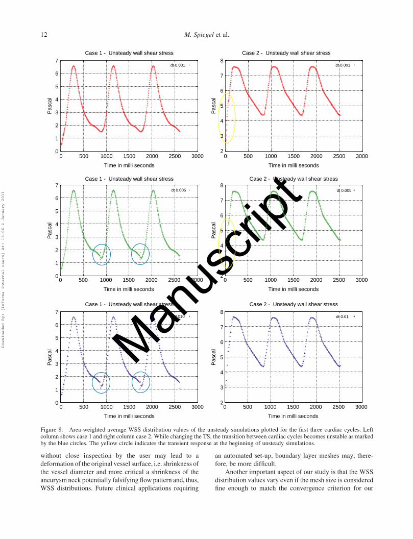
3.3 Unsteady simulation effects of varying TS size
The WSS distributions between the unsteady simulations
with different TS sizes were negligible, considering the
results at the moment of systole. This is shown in Figures 7
and 8. Table 5 summarises the differences in the area-
weighted average WSS distribution between the different
unsteady simulations averaged over the second and third
cardiac cycles. The CT significantly decreased as indicated
in Table 5, column 2. However, while increasing the
computational TS size for the Fluent CFD solver, there are
some important issues coming up: (a) the transition from
one cardiac cycle to the next cardiac cycle became
unstable in a sense of rapidly changing WSS distributions
as illustrated in Figure 8 blue circles and (b) regarding a
TS size of 0.001, the computation of each TS converged.
While increasing the TS size for unsteady simulation from
0.001 to 0.005 or 0.005 to 0.01 s, the number of non-
converged TS was also increasing. Consequently, the
number of iterations per TS had to be increased in order to
assure precise numerical simulation results. This led to
increased time requirement for computation. However, the
total time requirement for unsteady simulations performed
with 0.005 or 0.01 s significantly decreased compared to
the one with 0.001 s. The detailed time requirements for
each unsteady simulation are given in Table 5.
4. Discussion
In our study, a certain threshold of the mesh resolution was
required to obtain converged blood flow velocities and WSS
distributions. With a resolution lower than this threshold, the
velocity field and the WSS patterns fluctuated (see, Tables 3
and 4 grey areas and Figures 5 and 6). These results comply
with the work of Prakash and Ethier (2001), Dompierre et al.
(2002) and Lu et al. (2009) who stated that different mesh
resolutions lead to different flow predictions and only mesh-
independent flow solutions should be taken into account.
Once converged, WSS distributions obtained with either
tetrahedral or polyhedral meshes were of similar appearance.
Case 2
No BL
Tetrahedral Polyhedral
With BL
Tetrahedral Polyhedral
0.0 Pascal >45 Pascal
31696
75469
148625
8814
16795
30167
47311
100587
159797
26014
30435
44652
Figure 6. WSS distribution for polyhedral and tetrahedral meshes in comparison to boundary layer-based meshes. The numbers belowthe individual figures denote the number of cells of the mesh.
Table 5. Unsteady WSS simulation results – case 1 and case 2.
Wall shear stress
CT in h (TS in s.) Avg. StDev.
Case 1 12 (0.001) 3.3832 1.43954.5 (0.005) 3.2885 1.6721
2 (0.01) 3.2893 1.6874Case 2 7 (0.001) 5.9294 1.1007
4 (0.005) 5.9291 1.10192.5 (0.01) 5.9089 1.1019
CT and TS, computation time and time step.
M. Spiegel et al.10
Downloaded By: [informa internal users] At: 15:06 4 January 2011

Manus
cript
Polyhedral meshes may, therefore, be considered as a viable
alternative to tetrahedral meshes: (1) improved compu-
tational convergence as previously described by Peric
(2004). This becomes very important considering the clinical
applicability of CFD-based haemodynamic simulations.
Future clinical CFD-based diagnostic and treatment tools
have to perform fast and stable. Varying simulation
parameters for convergence optimisation is not feasible
during an intervention and (2) polyhedral elements resolve
significant WSS pattern with far less control elements in a
more homogeneous manner than tetrahedral meshes. The
reason for this lies in the way the WSS magnitude is
calculated which depends on two major aspects: firstly, only
those cell elements are considered which actually share a
face with the vessel boundary. Not all tetrahedral elements
located at the vessel boundary share necessarily an entire
face with the boundary – some may touch the boundary with
its corner, while all polyhedral elements located at the wall
share an entire face with the boundary itself. Secondly, the
distances of the considered tetrahedral centres are not equal
to the vessel wall leading to a more inhomogeneous WSS
appearance. Polyhedral meshes should be preferred over
tetrahedral meshes in future standardised clinical simu-
lations, since they have shown superior CFD properties in
terms of better convergence and less control elements which
directly lead to a shorter CT.
The usage of boundary layer leads to a more detailed
appearance of WSS distributions. This occurs because the
small prism elements approximate the vessel wall in
denser and accurate manner.
Accurately approximating WSS on the aneurysm wall
is of particular interest, as previous studies (Cebral, et al.
2005a; Jou et al. 2008) have demonstrated that aneurysms
exhibiting a WSS distribution with a higher portion of
lower values were more prone to expansion and perhaps
rupture. Although boundary layers lead to more details in
the WSS patterns, major features were already well
resolved in meshes without boundary layers. The drawback
of boundary layer meshes consists in their set-up resulting
in an increased complexity in user interaction. Correct
initiation of a boundary layer requires high smoothness and
spatial resolution of the vessel surface mesh to avoid highly
skewed elements at surface region exhibiting high
curvature, e.g. vessel bifurcations. Extensive smoothing
TS
0.00
1T
S0.
005
TS
0.01
Case 1
0.0 Pascal 43.0 Pascal 0.0 Pascal 15.5 Pascal
0.0 Pascal 61.5 Pascal
Case 2
Systole Diastole
Systole Diastole
Systole Diastole
Systole Diastole
Systole Diastole
Systole Diastole
0.0 Pascal 43.0 Pascal 0.0 Pascal 15.5 Pascal
0.0 Pascal 43.0 Pascal 0.0 Pascal 15.5 Pascal
TS
0.00
1T
S0.
005
TS
0.01
0.0 Pascal 61.5 Pascal
0.0 Pascal 61.5 Pascal
Figure 7. WSS distribution regarding unsteady simulation performed with different TS. The images show results at systole and diastole.Overall, there are no significant differences between the WSS patterns obtained from simulations with TS 0.001, 0.005 or 0.01 s.
Computer Methods in Biomechanics and Biomedical Engineering 11
Downloaded By: [informa internal users] At: 15:06 4 January 2011
Manus
cript
without close inspection by the user may lead to a
deformation of the original vessel surface, i.e. shrinkness of
the vessel diameter and more critical a shrinkness of the
aneurysm neck potentially falsifying flow pattern and, thus,
WSS distributions. Future clinical applications requiring
an automated set-up, boundary layer meshes may, there-
fore, be more difficult.
Another important aspect of our study is that the WSS
distribution values vary even if the mesh size is considered
fine enough to match the convergence criterion for our
7Case 1 - Unsteady wall shear stress Case 2 - Unsteady wall shear stress
Case 1 - Unsteady wall shear stress Case 2 - Unsteady wall shear stress
Case 1 - Unsteady wall shear stress Case 2 - Unsteady wall shear stress
6
4
3Pas
cal
Pas
cal
Pas
cal
Pas
cal
2
1
00 500 1000 1500 2000 2500 3000
Time in milli seconds
0 500 1000 1500 2000 2500 3000
Time in milli seconds
0 500 1000 1500 2000 2500 3000
Time in milli seconds
0 500 1000 1500 2000 2500 3000
Time in milli seconds
0 500 1000 1500 2000 2500 3000
Time in milli seconds
0 500 1000 1500 2000 2500 3000
Time in milli seconds
5
7
8
6
4
3
2
5
7
6
4
3Pas
cal
2
1
0
5
7
8
6
4
3
2
5
7
6
4
3Pas
cal
2
1
0
5
7
8
6
4
3
2
5
dt 0.001dt 0.001
dt 0.005 dt 0.005
dt 0.010 dt 0.01
Figure 8. Area-weighted average WSS distribution values of the unsteady simulations plotted for the first three cardiac cycles. Leftcolumn shows case 1 and right column case 2. While changing the TS, the transition between cardiac cycles becomes unstable as markedby the blue circles. The yellow circle indicates the transient response at the beginning of unsteady simulations.
M. Spiegel et al.12
Downloaded By: [informa internal users] At: 15:06 4 January 2011

Manus
cript
cases (see, Section 2). Since the true WSS distribution
cannot be measured in vivo, one has to be aware that the
WSS distribution simulations have an intrinsic uncertainty.
Within this study, this uncertainty for WSS values and
velocities ranges between 0.84 and 6.3% comparing
polyhedral vs. tetrahedral meshes with and without
boundary layers. This uncertainty has to be taken into
account clinically when making a quantitative statement
concerningWSS, blood velocity or blood flow pattern. The
key step in performing haemodynamic simulations, there-
fore, may be considered to generate a series of spatial
varyingmeshes and to postulate convergence oncevariation
of WSS falls in the range of 3–6%. If that is the case, then
themeshmay be considered to bewithin a convergence area
where mesh-independent simulation values can be
computed. Given this evaluation, we propose to omit the
usage of boundary layer for future clinical CFD application
at least in the research phase. Thiswill help to keep themesh
generation process simpler and easily automatable.
Unsteady simulations according to a patient-specific
cardiac cycle may lead to different WSS distributions as
obtained by steady simulations. However, unsteady
simulations induce a much higher computational demand
and thus lead to longer CT making a clinical CFD
application difficult during an intervention. The CT can be
minimised by either a reduction in the mesh resolution
(which may lead to non-reliable results) or an increase in
the computation TS governing the Fluent CFD solver for
solving the Navier–Stokes equation. Our experiments have
shown that an increase in the TS from 0.001 to 0.01 s does
not lead to any observable changes in the WSS distribution
at systole time, but a decrease in the CT by a factor of 6
(case 1) and 3 (case 2) (see, Table 3 column 2). An increase
in the TS, however, has to be regarded with suspicion
because there will be for sure a point once the TS is above a
certain value which leads to unstable or even disconverging
numerical solution. Overall, the first cardiac cycle should
not be used for evaluation or diagnosis, because of the
transient response of the corresponding Navier–Stokes
equations.
The results obtained during this study may be affected
due to several limitations of the analysis. Our assumptions
concerning the conducted CFD experiments differ from
the in vivo state in terms of rigid vessel walls, Newtonian-
based blood fluid and the determination of the boundary
conditions. The outflows of the patient-specific models are
defined as pressure outlet zero which does not have to
match with the real environment. There might be natural
resistances at the outflows. As with other computational
studies, it is assumed that these limitations have only
minor effects on the resulting flow pattern (Cebral et al.
2005b). Future work, however, has to focus on the
reduction in these limitations in the sense of validation
against in vivo measurements, perform this analysis with
much more cases and repeat it for the unsteady simulation.
5. Conclusion
This study has presented the first mesh granularity and mesh
independency analysis in the field of cerebral blood flow
simulation of aneurysms. Here, the focus is on the influence
of the CFD mesh, as aneurysms represent a complex
geometry. The aim was to determine how to reduce the CT.
Our results illustrate the importance of a well-founded
mesh granularity evaluation. A certain resolution is needed
to obtain valid and stable WSS patterns and velocity values.
However, even the CFD results of sufficient fine resolved
meshes show an uncertainty of 3–6%. Polyhedral meshes
are preferred for cerebral aneurysm CFD simulations due
to their advantages concerning better convergence, shorter
CT and high WSS accuracy. The usage of boundary layer
revealed that it does not significantly change the accuracy
of the WSS distributions, especially when using polyhedral
cell elements. Our variations of the TS for our unsteady
simulation experiments have illustrated that this leads to a
reduction in time without losing significant WSS
information at the systole time. This approach serves as a
first key step towards a future clinical CFD application
where the mesh generation process has to be automated.
The concepts and information presented in this paper
are based on research and are not commercially available.
Acknowledgements
The authors would like to thank Dr Ralf Kroeger (ANSYSGermany Inc.) for his advice and simulation support. The authorsgratefully acknowledge funding of the Erlangen Graduate Schoolin Advanced Optical Technologies (SAOT) by the GermanNational Science Foundation (DFG) in the framework of theexcellence initiative.
References
Cebral J, Castro M, Burgess J, Pergolizzi R, Sheridan M, PutmanC. 2005. Characterization of cerebral aneurysms forassessing risk of rupture by using patient-specific compu-tational hemodynamics models. Am J Neuroradiol.26:2550–2559.
Cebral J, Castro M, Appanaboyina S, Putman C, Millan D,Frangi A. 2005. Efficient pipeline for image-based patient-specific analysis of cerebral aneurysm hemodynamics:technique and sensitivity. IEEE Trans Med Imaging. 24(4):457–467.
Cebral J, Lohner R. 2005. Efficient simulation of blood flow pastcomplex endovascular devices using an adaptive embeddingtechnique. IEEE Trans Med Imaging. 24(4):468–476.
Cooperation F. 2007. Gambit 2.4 user’s guide. Wilmington, DE:du Pont de Nemours and Co.
Dompierre J, Vallet MG, Bourgault Y, Fortin M, Habashi WG.2002. Anisotropic mesh adaptation towards user-indepen-dent mesh-independent and solver-independent CFD part 3unstructured meshes. Int J Numer Methods Fluids.39:675–702.
Garimella R, Shephard M. 2000. Boundary layer meshgeneration for viscous flow simulation. Int J Numer MethodsEng. 49(2):193–218.
Computer Methods in Biomechanics and Biomedical Engineering 13
Downloaded By: [informa internal users] At: 15:06 4 January 2011

Manus
cript
Groden C, Laudan J, Gatchell S, Zeumer H. 2001. Three-dimensional pulsatile flow simulation before and afterendovascular coil embolization of a terminal cerebralaneurysm. J Cereb Blood Flow Metab. 21(12):1464–1471.
Hassan T, Ezura M, Timofeev E, Tominaga T, Saito T, TakahashiA, Takayama K, Yoshimoto T. 2004. Computationalsimulation of therapeutic parent artery occlusion to treatgiant vertebrobasilar aneurysm. Am J Neuroradiol.25(1):63–68.
Heran N, Song J, Namba K, Smith W, Niimi Y, Berenstein A.2006. The utility of DynaCT in neuroendovascularprocedures. Am J Neuroradiol. 27(2):330–332.
Hoi Y, Meng H, Woodward S, Bendok B, Hanel R, Guterman L,Hopkins L. 2004. Effects of arterial geometry on aneurysmgrowth: three-dimensional computational fluid dynamicsstudy. J Neurosurg. 101(4):676–681.
Jou L, Lee D, Morsi H, Mawad M. 2008. Wall shear stress onruptured and unruptured intracranial aneurysms at theinternal carotid artery. Am J Neuroradiol. 29(9):1761–1767.
Karmonik C, Arat A, Benndorf G, Akpek S, Klucznik R, MawadM, Strother C. 2004. A technique for improved quantitativecharacterization of intracranial aneurysms. Am J Neuror-adiol. 25(7):1158–1161.
Karmonik C, Klucznik R, Benndorf G. 2008. Blood flow incerebral aneurysms: comparison of phase contrast magneticresonance and computational fluid dynamics – preliminaryexperience. Rofo. 180(3):209–215.
Kato T, Indo T, Yoshida E, Iwasaki Y, Sone M, Sobue G. 2002.Contrast-enhanced 2D cine phase MR angiography formeasurement of basilar artery blood flow in posteriorcirculation ischemia. Am J Neuroradiol. 23:1346–1351.
Loehner R, Cebral J. 2000. Generation of non-isotropicunstructured grids via directional enrichment. Int J NumerMethods Eng. 49(2):219–232.
Lorensen WE, Cline H. 1987. Marching cubes: a high resolution3D surface construction algorithm. Comput Graph.21(4):163–169.
Lu B, Wang W, Li J. 2009. Searching for a mesh-independentsub-grid model for CFD simulation of gas–solid riser flows.Chem Eng Sci. 64:3437–3447.
Nader-Sepahi A, Casimiro M, Sen J, Kitchen N. 2004. Is aspectratio a reliable predictor of intracranial aneurysm rupture?Neurosurgery. 54(6):1343–1347.
Oaks W, Paoletti S. 2000. Polyhedral mesh generation. In:Proceedings ot the 9th International Meshing Round Table.New Orlean Louisiana: Sandia National Laboratoriesp. 57–66.
Peric M. 2004. Flow simulation using control volumes ofarbitrary polyhedral shape. In: ERCOFTAC bulletin;September, European Research Community on flow,turbulence combustion, p. 62.
Prakash S, Ethier CR. 2001. Requirements for mesh resolution in3D computational hemodynamics. J Biomech Eng.123:134–144.
Raghavan M, Ma B, Harbaugh R. 2005. Quantified aneurysmshape and rupture risk. J Neurosurg. 102(2):355–362.
Shojima M, Oshima M, Takagi K, Torii R, Hayakawa M, KatadaK, Morita A, Kirino T. 2004. Magnitude and role of wallshear stress on cerebral aneurysm computational fluiddynamic study of 20 middle cerebral artery aneurysms.Stroke. 35(11):2500–2505.
Spiegel M, Redel T, Zhang J, Struffert T, Hornegger J, GrossmanR, Doerfler A, Karmonik C. 2009. Tetrahedral andpolyhedral mesh evaluation for cerebral hemodynamicsimulation – a comparison. In: Multiscale BiomedicalEngineering (31st Annual International Conference of theIEEE EMBS Minneapolis, IEEE Society, Minneapolis, MN,USA, September 2–6). p. 2787–2790.
Steinman D, Milner J, Norley C, Lownie S, Holdsworth D. 2003.Image-based computational simulation of flow dynamics in agiant intracraniel aneurysm. Am J Neuroradiol.24(4):559–566.
Ujiie H, Tamano Y, Sasaki K, Hori T. 2001. Is the aspect ratio areliable index for predicting the rupture of a saccularaneurysm? Neurosurgery. 48(3):495–502.
Venugopal P, Valentino D, Schmitt H, Villablanca J, Vinuela F,Duckwiler G. 2007. Sensitivity of patient-specific numericalsimulation of cerebral aneurysm hemodynamics to inflowboundary conditions. J Neurosurg. 106(6):1051–1060.
Winn H, Jane J, Taylor J, Kaiser D, Britz G. 2002. Detection ofasymptomatic incidental aneurysms: review of 4568arteriograms. J Neurosurg. 96(1):43–49.
M. Spiegel et al.14
Downloaded By: [informa internal users] At: 15:06 4 January 2011


![Tetrahedral Mesh Generation for Deformable Bodies · Tetrahedral Mesh Generation for Deformable Bodies ... 2000; Hormann et al. 2002] to wrap subdivision surfaces around implicit](https://img.pdfslide.net/doc/110x75/611bd8b4e9a8473e5f0f61b8/tetrahedral-mesh-generation-for-deformable-bodies-tetrahedral-mesh-generation-for.jpg)