Simulation and Optimization of Spacecraft Re-entry Trajectories

A THESIS

SUBMITTED TO THE FACULTY OF THE GRADUATE SCHOOL

OF THE UNIVERSITY OF MINNESOTA

BY

Derrick G. Tetzman

IN PARTIAL FULFILLMENT OF THE REQUIREMENTS

FOR THE DEGREE OF

MASTER OF SCIENCE

Dr. William Garrard, Dr. Yiyuan Zhao

May 2010

© Derrick G. Tetzman 2010

i

Acknowledgements

I would first like to thank my advisor, Dr. William Garrard, for all of his time and advice

throughout the research process. I was very fortunate to have someone with the expertise

and perspective of Dr. Garrard in both giving me an outstanding space-related topic to

research, and in guiding me along the way with reality checks and insight. I am also

grateful for the financial award from Space Grant, which gave me valuable time to

complete this thesis.

Dr. Yiyuan Zhao played a crucial role in offering timely advice throughout the writing

process and in developing the optimization program. Dr. Zhao’s passion for his work,

constant enthusiasm and encouragement motivated and inspired me to aggressively

pursue understanding and implementing the algorithm. You can tell he loves his work

and loves working with students, as he always has a smile on his face, and he just radiates

optimism—in addition to optimization. I thank him for his time and assistance.

ii

Dedication

To my loving family and friends for all of their encouragement and support.

And

To the teachers and professors that helped motivate and inspire me to pursue my interest

in science, aviation and space, from the Minneapolis Public Schools, Minneapolis

Community and Technical College, and the University of Minnesota.

Thank you!

iii

Abstract

Parameter optimal control has the advantage of often being easier and faster to

solve than general optimal control methods, and may be better suited to the task of

spacecraft re-entry trajectory optimization. In this thesis, a parameter optimal control

algorithm is implemented in MATLAB® to optimize a 2-D re-entry trajectory simulated

via Simulink®. Simulation results are validated by comparison with data from the flight

of Apollo 4. Behavior of the algorithm is observed as it optimizes the control input under

different conditions without constraints applied. The performance of the optimization

program is observed as the complexity of the control input is increased up to the point

where constraints are required to continue the optimization process. Finally, a guide is

laid out for further development of the algorithm towards both pre-flight trajectory

planning and real-time control applications for re-entry.

iv

Table of Contents

List of Tables .............................................................................................................................. vi

List of Figures ............................................................................................................................ vii

Chapter 1: Introduction ............................................................................................................. 1

1.1 Motivations ...................................................................................................................... 1

1.2 Historical Background ..................................................................................................... 2

1.3 Parameter Optimal Control .............................................................................................. 2

1.4 Thesis Objectives ............................................................................................................. 3

1.5 Thesis Overview .............................................................................................................. 4

Chapter 2: Re-entry Model ........................................................................................................ 5

2.1 Overview .......................................................................................................................... 5

2.2 Coordinate Frames ........................................................................................................... 5

2.3 Equations of Motion ........................................................................................................ 9

2.4 Density Variation with Altitude ..................................................................................... 10

2.5 Variation in Gravity with Altitude ................................................................................. 11

2.6 Additional Calculations ................................................................................................. 12

2.7 Re-entry Heat Flux ......................................................................................................... 13

2.8 Wind Addition ............................................................................................................... 15

2.9 Earth Atmosphere Model Parameters ............................................................................ 16

Chapter 3: Simulation Studies ................................................................................................. 20

3.1 Simulation Parameters ................................................................................................... 20

3.2 Planetary entry via Simulink .......................................................................................... 21

3.3 Simulation Accuracy ...................................................................................................... 23

3.4 Step-Solver Study .......................................................................................................... 23

3.5 Apollo 4 Case Study ...................................................................................................... 24

3.6 Correction of Stagnation Point Heating Constant .......................................................... 27

3.7 Comparison of Results with Apollo 4 Flight Data ......................................................... 27

3.8 Wind Addition ............................................................................................................... 34

Chapter 4: Problem Formulation ............................................................................................ 38

4.1 Problem Definition and Description .............................................................................. 38

4.2 Application of Parameter Optimal Control to Re-entry ................................................. 39

v

4.3 Optimization Study ........................................................................................................ 41

4.3.1 Validation ....................................................................................................................... 41

4.3.2 Program Robustness ....................................................................................................... 42

4.3.3 Effects of Wind Addition and Increasing the Number of Intervals ............................... 42

4.3.4 Constraint addition ......................................................................................................... 43

4.3.5 Apollo 4 Conditions ....................................................................................................... 44

Chapter 5: Numerical Methods ............................................................................................... 45

5.1 Control Input and Constraint Information via Simulink ................................................ 45

5.2 Algorithm Implementation ............................................................................................. 46

5.3 Wind Addition ............................................................................................................... 47

Chapter 6: Results..................................................................................................................... 49

6.1 Summary ........................................................................................................................ 49

6.1.1 Test Parameters .............................................................................................................. 49

6.2 Validation ....................................................................................................................... 51

6.3 Program Robustness ....................................................................................................... 56

6.4 Effects of Wind Addition and Increasing the Number of Intervals ............................... 62

6.5 Constraint addition ......................................................................................................... 69

6.6 Apollo 4 Conditions ....................................................................................................... 73

Chapter 7: Conclusions ............................................................................................................ 74

7.1 Summary ........................................................................................................................ 74

7.2 Simulation and Optimization Program Development .................................................... 74

7.3 Additional Problem Formulations .................................................................................. 76

7.4 Stochastic Re-entry ........................................................................................................ 77

7.5 Simulating Mars and Titan ............................................................................................. 79

7.6 Suggested References for Further Research .................................................................. 81

Epilogue ..................................................................................................................................... 83

References .................................................................................................................................. 86

Appendix A: Equations of Motion Proof ................................................................................ 89

Appendix B: Heat Flux Derivation .......................................................................................... 94

Appendix C: Exponential Density Model ............................................................................... 97

Appendix D: Opt. Study Results Tables ................................................................................. 99

Appendix E: Optimization Code ........................................................................................... 102

Appendix F: Simulink Model ................................................................................................. 108

vi

List of Tables

Table 2.1 Parameters for the Earth model including mole fractions of the three major

constituents of the atmosphere [8] [13]. ........................................................................... 17

Table 3.1 Notable parameters from the flight of Apollo 4 used in simulations................ 26

Table 6.1 Baseline or “undershoot” test parameters. ........................................................ 50

Table 6.2 Hardware and software specifications. ............................................................. 50

Table 6.3 Results of changing the initial step. .................................................................. 61

Table 7.1 Parameters for the Mars model including mole fractions of the three major

constituents of the atmosphere [25] [26]. ......................................................................... 80

Table 7.2 Parameters for the Titan model including mole fractions of the three major

constituents of the atmosphere [27] [28]. ......................................................................... 81

Table D.1 Results from Chapter 6 undershoot case. ......................................................... 99

Table D.2 Results from Chapter 6 for the overshoot case. ............................................. 100

Table D.3 Results from Chapter 6 for the undershoot with wind case. .......................... 101

vii

List of Figures

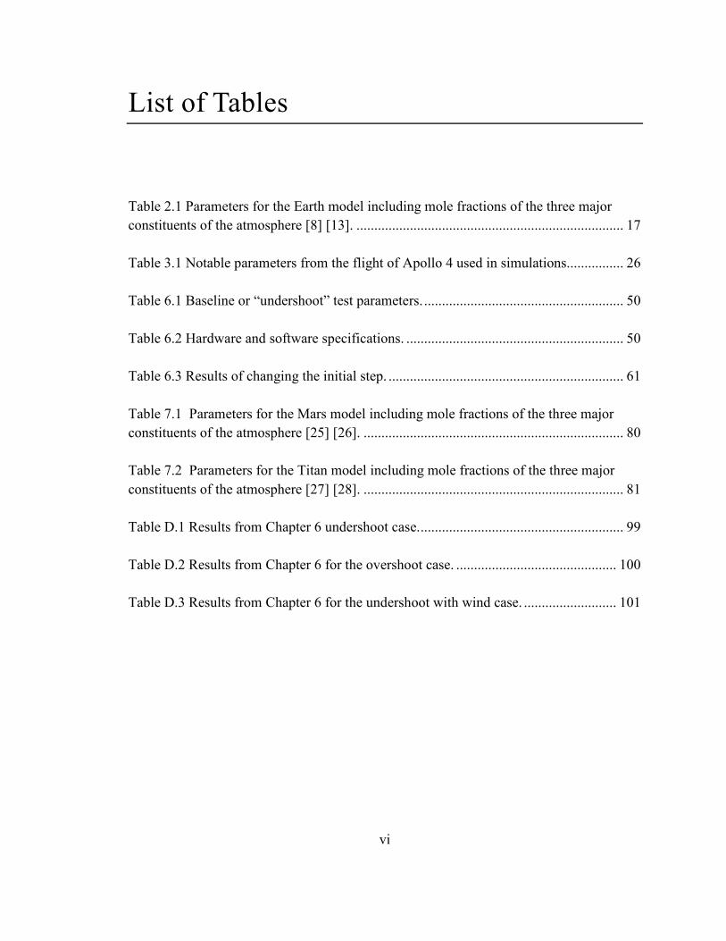
Figure 1.1 Control input of a general optimal control problem vs. a parameter optimal

control problem. .................................................................................................................. 3

Figure 2.1 Motion of spacecraft relative to planet’s fixed axis. ......................................... 7

Figure 2.2 A snapshot of the body and local frame motion about the fixed frame of the

planet. .................................................................................................................................. 8

Figure 2.3 Wind vector addition. ...................................................................................... 15

Figure 2.4 Error between isothermal model and tabulated density values for each

kilometer of the 1976 standard atmosphere. ..................................................................... 18

Figure 2.5 Comparison between isothermal model and tabulated density values for each

kilometer of the 1976 standard atmosphere (for a different perspective). ........................ 19

Figure 3.1 Process diagram for a single time step in the Simulink program. .................. 22

Figure 3.2 The Apollo 4 Command Module CM-017 being hoisted above its recovery

ship, the U.S.S. Bennington [14]. ..................................................................................... 25

Figure 3.3 Apollo 4 vertical lift to drag ratio vs. ground elapsed time in seconds. .......... 29

Figure 3.4 Approximated control input using average values from [14] at 30 s intervals.

........................................................................................................................................... 29

Figure 3.5 Simulated trajectory after applying the approximate Apollo 4 control input

compared with the reconstructed trajectory of Apollo 4 from flight data. ....................... 30

Figure 3.6 Stagnation point heat flux vs. horizontal range from the simulation .............. 31

Figure 3.7 Deceleration load factor vs. range for the simulation...................................... 32

viii

Figure 3.8 Apollo 4 deceleration loading vs. ground elapsed time from [14], for

comparison with Figure 3.7. ............................................................................................. 33

Figure 3.9 Simulated trajectories at constant L/D for calm and constant wind

conditions. ......................................................................................................................... 34

Figure 3.10 Plot of horizontal wind velocity from the HWM93 wind model at the place

and time of year of the Apollo 4 splashdown. .................................................................. 35

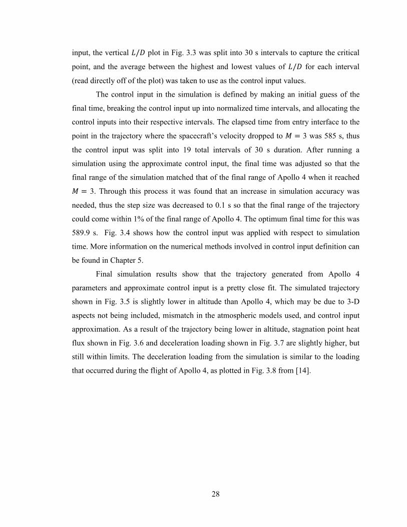
Figure 3.11 Simulated trajectories at constant L/D for calm (dotted line) and wind profile

conditions. ......................................................................................................................... 36

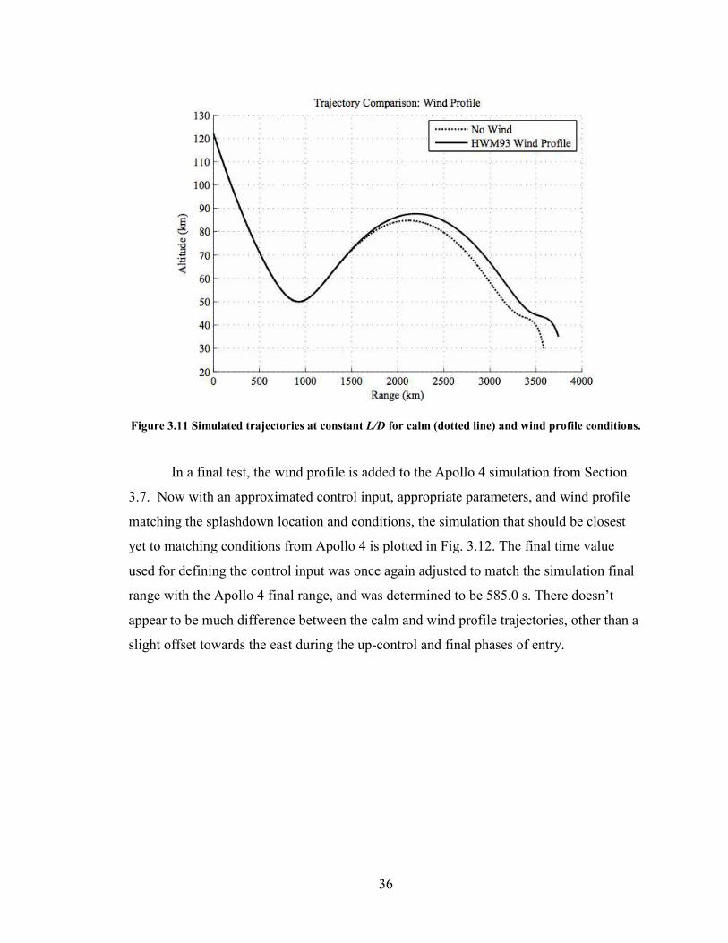
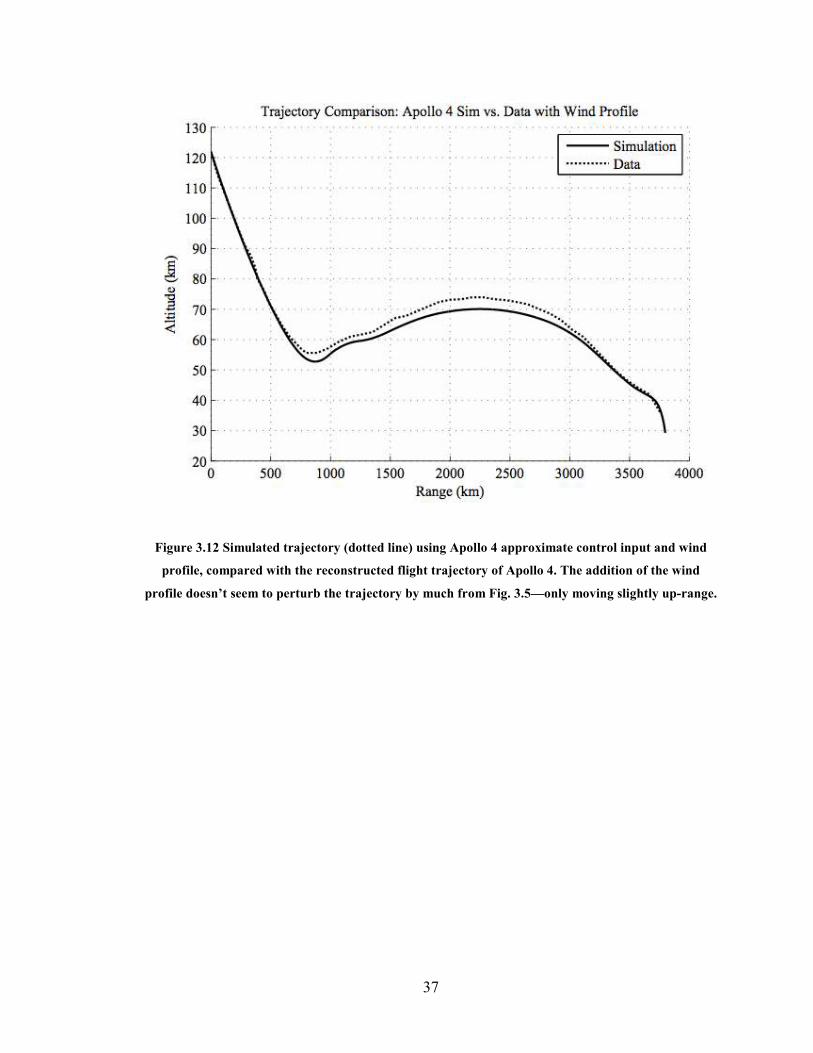
Figure 3.12 Simulated trajectory (dotted line) using Apollo 4 approximate control input

and wind profile, compared with the reconstructed flight trajectory of Apollo 4. ........... 37

Figure 4.1 Predicted results for increasing n. ................................................................... 43

Figure 4.2 Predicted ability of program to handle constraints as n is increased. .............. 44

Figure 5.1 “Interval” embedded m-function block within the Simulink model. ............. 46

Figure 5.2 “hwindv” embedded m-function block within the Simulink model. .............. 48

Figure 6.1 Cost function progress vs. loop iteration for � � 1, baseline parameters. ...... 52

Figure 6.2 Cost function progress vs. final range � � 1, baseline parameters. ................ 53

Figure 6.3 Final time progress vs. loop iteration � � 1, baseline parameters. ................. 54

Figure 6.4 Optimized control input vs. time � � 1, baseline parameters. ........................ 55

Figure 6.5 Optimized trajectory for � � 1, baseline parameters (solid line), compared

with the trajectory of Apollo 4 as reconstructed in Chapter 3. ......................................... 56

Figure 6.6 Final time progress vs. loop iteration for � � 1, overshoot parameters. ......... 57

Figure 6.7 Cost function progress vs. final range � � 1, overshoot parameters. ............. 58

ix

Figure 6.8 Optimized trajectory for � � 1, overshoot parameters, compared with the

trajectory of Apollo 4 as reconstructed in Chapter 3. ....................................................... 59

Figure 6.9 Optimized control input vs. time for � � 3, overshoot parameters compared

with the baseline optimized control input for � � 3. ........................................................ 60

Figure 6.10 Optimized control input vs. time for � � 6, baseline parameters compared

with the wind optimized control input for � � 6. ............................................................. 63

Figure 6.11 Computational cost in terms of the number of iterations required to find the

optimal control input. ........................................................................................................ 65

Figure 6.12 Computation cost in terms of program run time to find the optimal control

input. ................................................................................................................................. 65

Figure 6.13 Optimization progress after 100 loop iterations for 1-5 intervals used. . ...... 66

Figure 6.14 Optimization progress after 140 loop iterations for 1-5 intervals used. ....... 67

Figure 6.15 Optimization progress after 180 loop iterations for 1-6 intervals used. ........ 67

Figure 6.16 Baseline trajectories from n = 2 through n = 6 plotted on the same graph, as

well as the Apollo 4 trajectory for comparison. ................................................................ 68

Figure 6.17 Zoomed-in view of trajectories from n = 2 through n = 6 from Figure 6.16

........................................................................................................................................... 69

Figure A.1 Geometry of body frame rotation. .................................................................. 91

Figure F.1 Gravity and density calculations. .................................................................. 108

Figure F.2 Interval m-function, absolute acceleration and flight path angular velocity

equations. ........................................................................................................................ 109

Figure F.3 Calculations for vertical and horizontal components of velocity, freestream

velocity, and stag. pt. heat flux. ...................................................................................... 110

Figure F.4 Conversion of range an altitude from m to km, mach number and dynamic

pressure calculations. ...................................................................................................... 111

x

Figure F.5 Loading calculation, heat flux and flight path angle fed to workspace, and stop

simulation conditions. ..................................................................................................... 112

Figure F.6 Correction to velocity and flight path angle for wind. .................................. 113

1

Chapter 1: Introduction

1.1 Motivations

Spacecraft atmospheric entry remains one of the most challenging, dangerous and

extreme phases of spaceflight. We were reminded of this fact on February 1st, 2003, when

seven astronauts lost their lives during the break up of the space shuttle Columbia during

re-entry. The crash of the Genesis space capsule on September 9th

, 2004 due to a para-

chute malfunction demonstrated the risk to some of our most valued and expensive

scientific payloads—those involving sample return. Safety is of utmost importance in

re-entry, as the result of failure is highly disastrous and costly in our furthered under-

standing of our solar system, in dollars, and in human lives. While much progress in re-

entry vehicle and trajectory design has been made in the last half century of spaceflight,

further improvements in our current systems are as important as ever.

In the design of a re-entry trajectory, there is much to be considered. With the

characteristics of the spacecraft and the planetary environment in mind, an optimal

trajectory maximizes the performance of the spacecraft in meeting mission objectives

while at the same time minimizing the negative effects of the environment such that

uncertainty is accounted for, and the physical limitations of the spacecraft and its payload

are not exceeded. To accomplish this, algorithms are implemented in both pre-flight

trajectory planning and in real-time control during re-entry to find the optimal control

input that in turn generates an optimal trajectory achieving the mission objectives.

In the case of real-time optimal control, a solution must be generated as quickly as

possible so that the system can adequately adapt to rapidly changing conditions. This

thesis presents an optimization study of a parameter optimal control algorithm that when

applied to re-entry, may help address this problem.

2

1.2 Historical Background

Advances in numerical methods for trajectory optimization have paralleled

advances in space exploration and computer processing power [1]. For re-entry, solution

methods typically involve solving two-point boundary value problems (TPBVPs) directly

using non-linear programming and shooting methods. Solving these boundary value

problems is computationally intensive, and may take too long to be used in real-time.

Bulirsch [2, pp. 565] presented early results for “an Apollo type vehicle” using these

methods. References [3] through [5] further describe the application of solving TPBVPs

for re-entry trajectories of the X-38 Crew Return Vehicle (cancelled in 2002) [3, pp.

295], and of the space shuttle [4, pp. 133] [5].

1.3 Parameter Optimal Control

Instead of finding a control history ���� that minimizes some cost function I

(determined by the mission objectives and/or spacecraft design limitations) as in the

general optimal control problem, parameter optimal control instead seeks to optimize a

control input by approximating it as several piecewise-defined segments, whose duration

depend upon the final time and number and spacing of intervals used. This transforms the

optimal control problem into a parameter optimization problem where the unknowns are:

1) the endpoints of the intervals, �, 2) the vector containing the control input for each

interval, ��, and 3) the final time �. This has the potential benefit of making the optimal

control problem simpler to solve, but still requires numerical solution methods via non-

linear programming. A comparison between general and parameter optimal control

methods is depicted in Fig. 1.1. A more comprehensive description of this can be found

in Hull [6, pp. 350]. In addition to the benefit of lower computational cost, this method is

more fitting spacecraft trajectory correction because it requires less update to the control

input, while general methods require continuous update.

3

Figure 1.1 Control input of a general optimal control problem (left) vs. a parameter optimal control

problem (right).

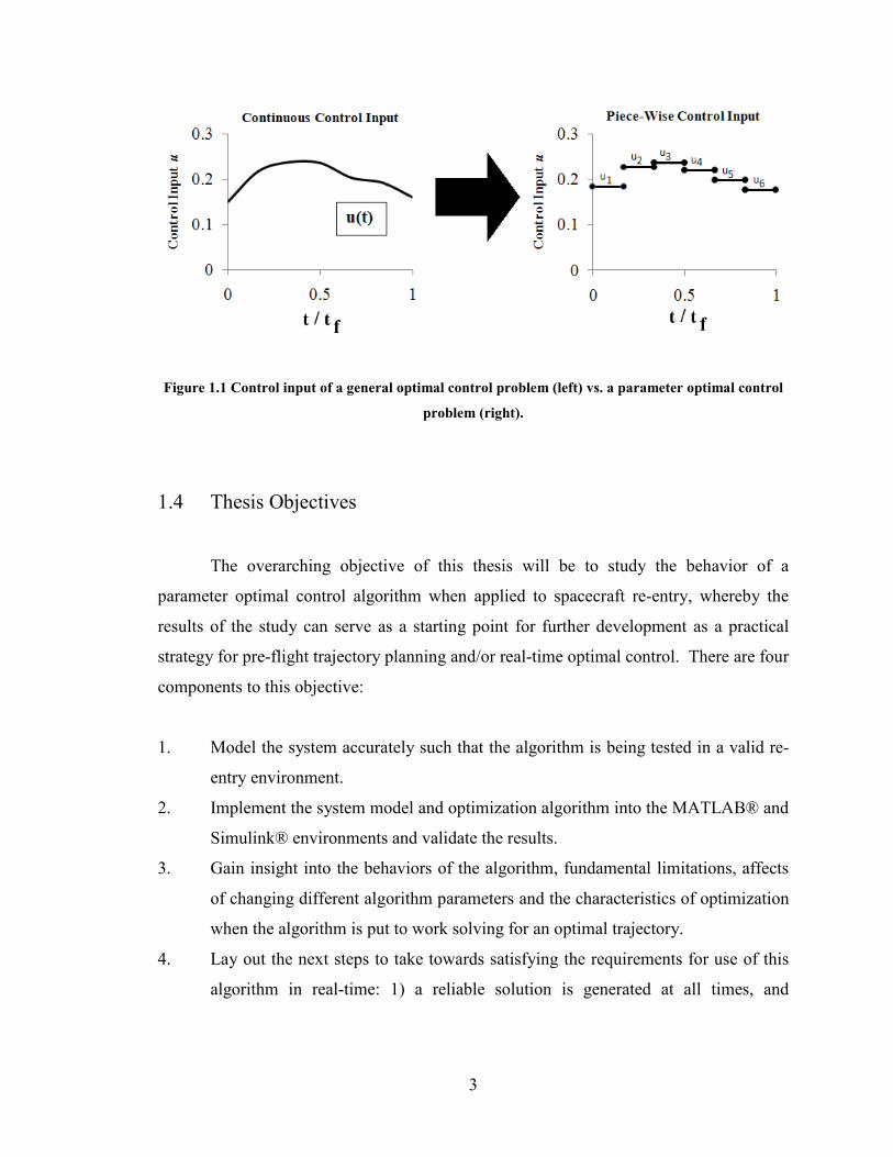
1.4 Thesis Objectives

The overarching objective of this thesis will be to study the behavior of a

parameter optimal control algorithm when applied to spacecraft re-entry, whereby the

results of the study can serve as a starting point for further development as a practical

strategy for pre-flight trajectory planning and/or real-time optimal control. There are four

components to this objective:

1. Model the system accurately such that the algorithm is being tested in a valid re-

entry environment.

2. Implement the system model and optimization algorithm into the MATLAB® and

Simulink® environments and validate the results.

3. Gain insight into the behaviors of the algorithm, fundamental limitations, affects

of changing different algorithm parameters and the characteristics of optimization

when the algorithm is put to work solving for an optimal trajectory.

4. Lay out the next steps to take towards satisfying the requirements for use of this

algorithm in real-time: 1) a reliable solution is generated at all times, and

4

2) solutions are generated quickly. All of the conclusions reached from the

optimization study are intended to serve as a guide for suitable further research

All experiments, results, and conclusions reached in Chapters 3, 6, and 7 trace back to

one of these component-objectives.

1.5 Thesis Overview

In Chapter 2 we will begin with an overview of the model used for simulation of

re-entry and the physics from which it is derived. In Chapter 3, the means of simulating

re-entry using this model through MATLAB and Simulink, and the methods of validating

the simulations will be described. The full optimization problem will be formulated in

Chapter 4, including a description of the parameter optimal control algorithm as well as a

list of the tests to be done to analyze it. The full implementation of this algorithm in the

MATLAB and Simulink environment will be described in Chapter 5: Numerical

Methods. Results of the tests laid out in Chapter 4 are presented and discussed in Chapter

6. Finally, conclusions reached from the results are discussed in Chapter 7, along with a

guide for relevant future research to improve and build upon the optimization program

developed.

5

Chapter 2: Re-entry Model

2.1 Overview

A simplified two-dimensional, three degree-of-freedom re-entry model is used for

re-entry simulation. This chapter lays out the differential equations describing

atmospheric characteristics, motion of the spacecraft, and stagnation point heat flux

during re-entry, and the assumptions needed to derive them. Note that while the case

study described in Chapter 3 uses this model to simulate re-entry for a capsule, it can be

used for any space vehicle. This model is not accurate enough to be used in detailed

spacecraft design, but is sufficient for broad research and trajectory analysis.

2.2 Coordinate Frames

In order to simplify the complex environment of re-entry so that this model can be

constructed, reasonable assumptions must be made. Assumptions listed in [7, pp. 275] are

the basis for this model. However, the application of this model requires more accuracy,

thus not all of the assumptions in [7] are used.

For this model, the following assumptions are made for the equations of motion:

1. Spherical planet.

2. No initial acceleration.

3. Non-rotating planet—sets the coordinate frame of the planet as fixed. The velocity of

the spacecraft is then absolute with respect to the planet.

6

Additional assumptions necessary to approximate atmospheric density variation with

altitude, variation in gravitational acceleration with altitude, and the stagnation point heat

flux on the spacecraft will be listed in subsequent sections.

Three coordinate frames are necessary to fully describe the motion of the

spacecraft in this model: 1) a fixed frame, with its origin at the center of the planet, 2) a

moving local reference frame with its origin at the spacecraft’s center of gravity, and

vertical axis parallel to the vector � extending from the center of the planet to the center

of gravity of the spacecraft, and 3) a rotating body frame for the spacecraft with its origin

also at the center of gravity, tangential axis parallel to the velocity vector, and normal

axis pointing down towards the planet. Figure 2.1 depicts the motion of the spacecraft

about the fixed frame, and Figure 2.2 depicts the motion of the local and body frames, as

well as the orientation of the force vectors and velocity vector. These relationships will

prove important in deriving the equations of motion for the spacecraft during re-entry.

7

Figure 2.1 Motion of spacecraft relative to planet’s fixed axis. Altitudes above the surface are

exaggerated in scale to show detail. The trajectory begins at the altitude of entry interface, � � � , and ������ � . The vector �� extends from the planet’s center to the CG of the spacecraft, and has a magnitude equal to the sum of the planet’s radius R and altitude above the surface h. The angle �

extends from ������ to the spacecraft’s current location at ��.

8

Figure 2.2 A snapshot of the body and local frame motion about the fixed frame of the planet. Lift,

drag, and gravitational forces, as well as the absolute velocity vector, are also shown in relation to the

frames. The y-axis of the local frame is defined to be parallel with ��, and the tangential axis of the body frame is defined to be parallel with that of the velocity vector. The flight path angle � is defined as the angle between the velocity vector and the local horizontal (or horizon), and is shown here in a

negative orientation—experienced if the spacecraft is in an “up control” phase of re-entry.

9

2.3 Equations of Motion

The differential equations defining the spacecraft’s entry trajectory are derived

from the lift and drag forces acting on the spacecraft with respect to the body frame, as

well as from the absolute velocity with respect to the local frame. Full derivations of

these equations can be found in Appendix A.

There are four differential equations that are essential for simulating the entry

trajectory. The horizontal velocity

�� � �cos�, (2.1)

and vertical velocity

�� � �sin�, (2.2)

are both defined with respect to the local frame. The absolute acceleration

�� � ! "#$%& ' (sinγ , (2.3)

where B is the ballistic coefficient

) � +,-. , (2.4)

is derived from summing the forces in the body frame. An additional assumption must be

made to compute this:

4. Drag coefficient /0 is constant for the spacecraft during re-entry.

10

Finally, the flight path angular velocity

�� � ! "#12 03 4%& ' 5 6789

# ! # 678 9: , (2.5)

is derived from both the sum of forces in the body frame as well as geometry and

kinematic relationships. This expression for �� also takes into account the rotation of the

local frame caused by the curvature of the planet. With only these four equations of

motion and supporting calculations for density and gravitational variation with altitude, a

re-entry trajectory can be simulated.

2.4 Density Variation with Altitude

In order to calculate the density at a given altitude continuously with the

equations of motion, an exponential model for density variation is derived from the

equation of hydrostatic equilibrium and the following assumptions:

5. Gas composing the atmosphere acts as ideal gas.

6. Isothermal atmosphere.

7. The atmosphere is homogeneous in its constituent gasses, thus having a molecular

weight ; that is constant with altitude.

The result of the derivation laid out in Appendix C is

< � <=>?@ABC

, (2.6)

where <= is the density at � � 0, and E is the scale height,

E � : FG 5H , (2.7)

11

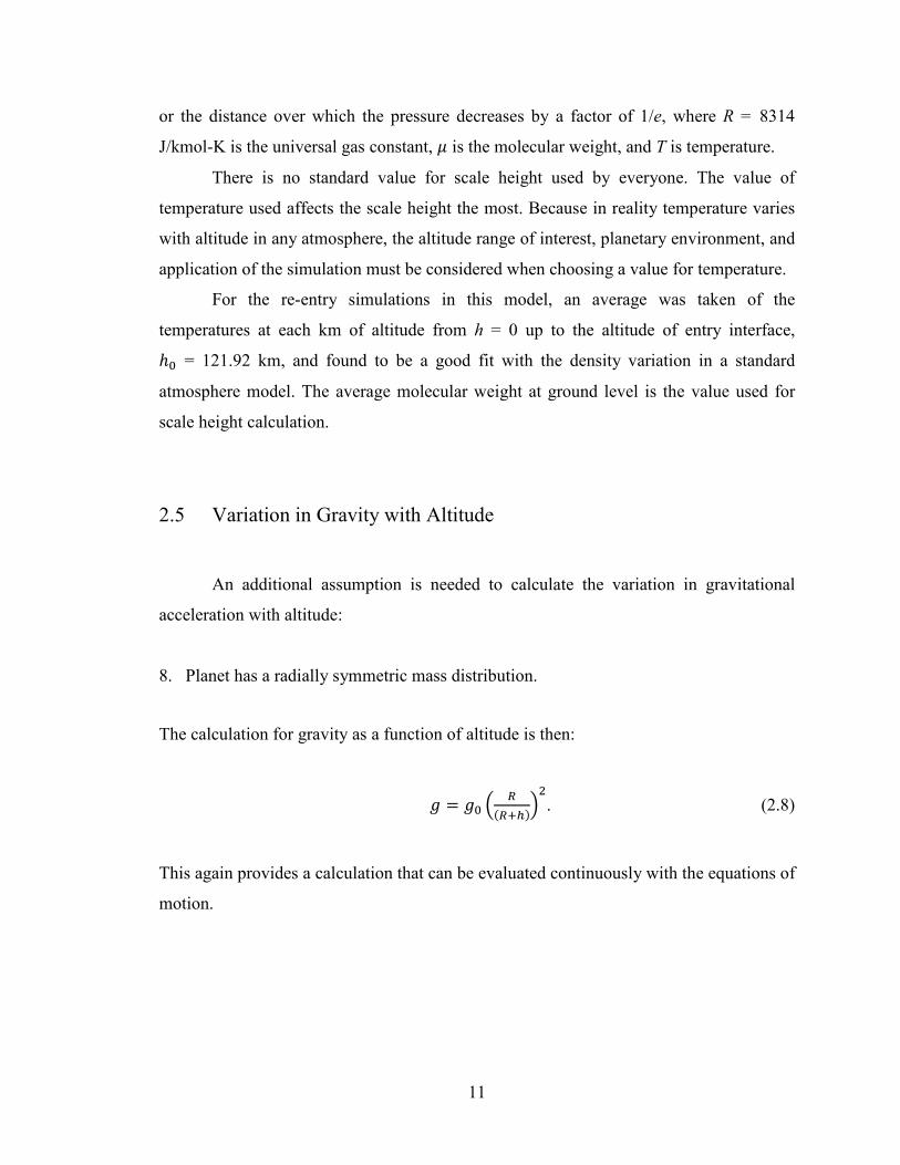
or the distance over which the pressure decreases by a factor of 1/e, where R = 8314

J/kmol-K is the universal gas constant, ; is the molecular weight, and T is temperature.

There is no standard value for scale height used by everyone. The value of

temperature used affects the scale height the most. Because in reality temperature varies

with altitude in any atmosphere, the altitude range of interest, planetary environment, and

application of the simulation must be considered when choosing a value for temperature.

For the re-entry simulations in this model, an average was taken of the

temperatures at each km of altitude from h = 0 up to the altitude of entry interface,

�= = 121.92 km, and found to be a good fit with the density variation in a standard

atmosphere model. The average molecular weight at ground level is the value used for

scale height calculation.

2.5 Variation in Gravity with Altitude

An additional assumption is needed to calculate the variation in gravitational

acceleration with altitude:

8. Planet has a radially symmetric mass distribution.

The calculation for gravity as a function of altitude is then:

( � (= ? :�:IJ�C

%. (2.8)

This again provides a calculation that can be evaluated continuously with the equations of

motion.

12

2.6 Additional Calculations

There are a few other equations of importance in trajectory analysis. One is the

speed of sound

K � L�MN, (2.9)

where � is the specific heat ratio. After applying assumptions 5 and 6, � and a are

constant with respect to altitude. The Mach number is then

O � #P . (2.10)

Mach number is only needed to determine if the spacecraft is at the threshold of

hypersonic flight, which will be assumed here as O � 3. The dynamic pressure

RS � T% <�%, (2.11)

may also be of interest. However, the biggest limiting factors in trajectory design stem

from the extreme amount of heating produced during re-entry, described in the next

section, and the deceleration load factor

U � #�5H,WXYZA , (2.12)

where (=,[P\]J is the acceleration of gravity specific to Earth at ground level.

13

2.7 Re-entry Heat Flux

Heat transfer to the spacecraft during re-entry must be considered when

simulating and analyzing its trajectory. Heating induced from the hypersonic flow around

the spacecraft heavily influences its design, due to limitations of the materials used to

shield it as well as what the payload can tolerate, be it manned or unmanned. In turn,

these limitations often constrain the optimum trajectory of the spacecraft.

The large amount of potential and kinetic energy of a re-entering spacecraft is

dissipated as heat as it enters the atmosphere. The shock wave created by a spacecraft

moving at high hypersonic velocities induces extremely high temperatures that dissociate

air molecules into ions [8]. Total drag on the spacecraft is the sum of friction drag and

pressure drag. Because friction drag will produce much higher levels of heating than

pressure drag, a blunt shape is desired for the component of the spacecraft most directly

facing the oncoming flow, or the nose (in the case of a capsule spacecraft, this would be

the heat shield). Most of the heat is carried away by the detached bow shock wave [9],

with the remainder of the heat transferred to the spacecraft through convection and

radiation. Temperature gradients are proportional to the surface heat flux, and vary with

position along the surface [9].

For a blunt-body, the maximum heat flux can be assumed to occur at the

stagnation point. Though there are some exceptions to this, for the intents and purposes of

this model stagnation point heating is our main concern. Fay and Riddle originally

tackled this problem in the 1950s [10], then further investigated for re-entry applications

by Allen and Eggers [9], and by Sutton and Graves during the Apollo era for different gas

mixtures [11].

14

From Allen and Eggers [9, pp. 5], the following assumptions are made to derive a

simple differential equation of the heat flux at the stagnation point:

9. Assume convective heat transfer is the only source of heat transfer (radiation

negligible across boundary layer).

10. Assume perfect gas model through the shock wave.

11. Neglect gaseous imperfections (specifically dissociation).

12. Neglect shock-wave boundary layer interaction.

13. Reynolds’ analogy is applicable.

14. The Prandtl number is unity.

15. N _ N∞, and N _ N .

Where N∞, N , and N are the freestream, boundary layer edge (at the stagnation point),

and wall temperatures, respectively. The result of the derivation laid out in Appendix B is

R� � ,#aL"L:b , (2.13)

where Mc is the nose radius (radius of curvature at the stagnation point), and C is a

constant dependant on the gas composing the atmosphere. Values for C suggested by [12]

are 1.83 d 10@f kgT %3 m@T for Earth and 1.89 d 10@f kgT %3 m@T for Mars. However, the

assumptions of Allen and Eggers begin to break down at entry speeds approaching

around 6 km/s due to gaseous imperfections and specifically, disassociation. To take this

into account, the value used for C will be adjusted to approximately match actual

re-entry data.

15

2.8 Wind Addition

A modification must be made to the velocity, flight path angle, heat flux, and

loading equations to account for horizontal wind. This comes from the vector addition of

absolute velocity with the wind vector, and is depicted in Figure 2.3. An additional

calculation will also need to be made to compute the spacecraft’s velocity relative to the

freestream. This will become crucial in heat flux and loading calculations.

Figure 2.3 Wind vector addition.

Using components of velocity as a means of vector addition,

�� � � cos � ' j � � ′ cos � ′ (2.14)

k� � � sin � � � ′ sin � ′, (2.15)

where j is the wind, � ′ is the resultant velocity, and � ′ is the resultant flight path angle,

the velocity update becomes

� ′ � # 678 9Il678 9′

. (2.16)

16

The update in flight path angle is derived from the equation for tan� ′,

� ′ � tan@T o 8pq 9678 9Ir

st . (2.17)

Freestream velocity

��∞ � L�� cos � ! j�% ' �� sin ��% , (2.18)

will then replace absolute velocity in the acceleration, heating, loading, and dynamic

pressure calculations.

2.9 Earth Atmosphere Model Parameters

Planetary constants used in this model are from the 1976 U.S. Standard

Atmosphere [13] as well as [8]. The 1976 model has been widely used, and our

knowledge of the Earth’s atmosphere has not changed very much since it was created.

The temperature used to calculate scale height was found by averaging the temperature at

each kilometer of altitude from sea level up to 123 km (just above the standard entry

interface altitude of 121.92 km). Molecular weight was calculated from the mole frac-

tions of the three major constituents of the atmosphere as listed in [13]. Table 2.3 lists all

parameters needed to simulate Earth entry.

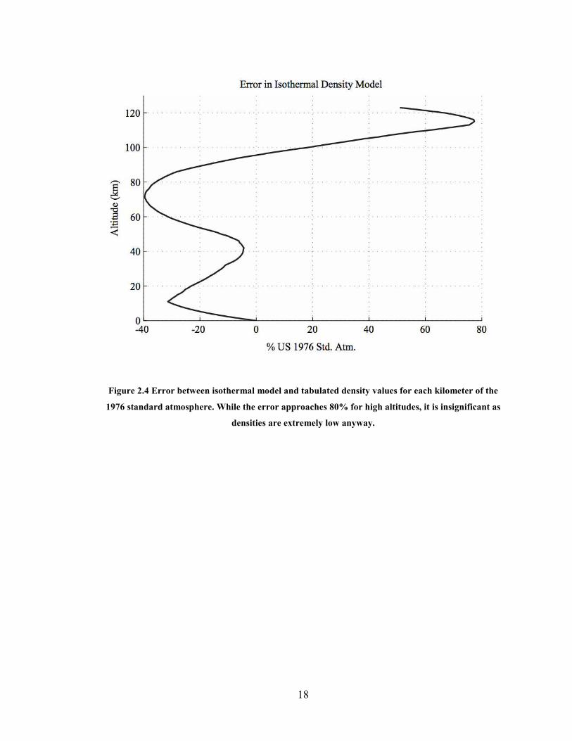
Values for scale height for Earth as listed by other sources typically fall

somewhere between 6-8 km. Using the values listed in Table 2.1, scale height was

calculated to be 6.93 km, which is close to the value used by Allen and Eggers, 6.7 km.

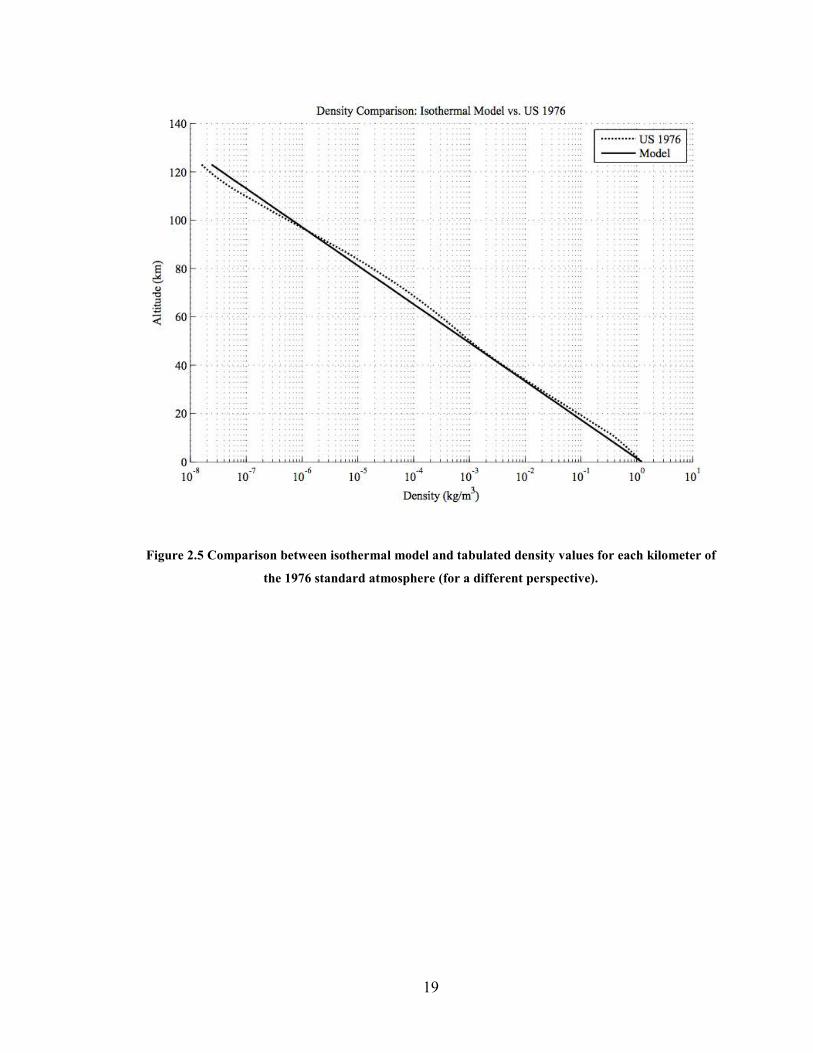
The error between the computed density from the exponential model and the values listed

for density in [13] is plotted in Fig. 2.4, and just to show a different perspective, a

comparison between the exponential model and [13] is plotted in Fig. 2.5.

17

Table 2.1 Parameters for the Earth model including mole fractions of the three major constituents of

the atmosphere [8] [13].

Parameter Value

R 6378 km

E 6.93 km

�= 121.92 km

<= 1.225 kg/m%

(= 9.81 m/s%

� 1.4

T 236.715 K

; 28.95 kg/kmol

uv$ 0.78084

uw$ 0.209476

ux\ 0.00934

18

Figure 2.4 Error between isothermal model and tabulated density values for each kilometer of the

1976 standard atmosphere. While the error approaches 80% for high altitudes, it is insignificant as

densities are extremely low anyway.

19

Figure 2.5 Comparison between isothermal model and tabulated density values for each kilometer of

the 1976 standard atmosphere (for a different perspective).

20

Chapter 3: Simulation Studies

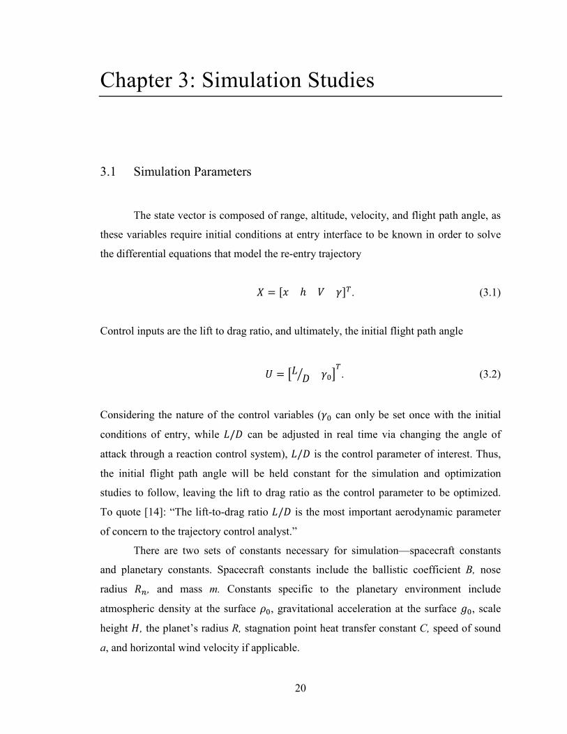
3.1 Simulation Parameters

The state vector is composed of range, altitude, velocity, and flight path angle, as

these variables require initial conditions at entry interface to be known in order to solve

the differential equations that model the re-entry trajectory

u � y� � � �zF. (3.1)

Control inputs are the lift to drag ratio, and ultimately, the initial flight path angle

{ � |U }3 �=~F. (3.2)

Considering the nature of the control variables (�= can only be set once with the initial

conditions of entry, while U/} can be adjusted in real time via changing the angle of

attack through a reaction control system), U/} is the control parameter of interest. Thus,

the initial flight path angle will be held constant for the simulation and optimization

studies to follow, leaving the lift to drag ratio as the control parameter to be optimized.

To quote [14]: “The lift-to-drag ratio U/} is the most important aerodynamic parameter

of concern to the trajectory control analyst.”

There are two sets of constants necessary for simulation—spacecraft constants

and planetary constants. Spacecraft constants include the ballistic coefficient B, nose

radius Mc, and mass m. Constants specific to the planetary environment include

atmospheric density at the surface <=, gravitational acceleration at the surface (=, scale

height E, the planet’s radius R, stagnation point heat transfer constant C, speed of sound

a, and horizontal wind velocity if applicable.

21

3.2 Planetary entry via Simulink

Implementation of the re-entry model discussed in Chapter 2 is done through

MATLAB and Simulink. Widely used for dynamic system modeling and control theory

applications, the visual programming interface of Simulink allows the programmer to

easily set up and view the flow of a model. The MATLAB and Simulink code used to

simulate re-entry trajectories can be found in Appendices E and F, respectively, as part of

the parameter optimal control program.

The differential equations describing the equations of motion, and the calculations

required to compute the stagnation point heat flux, density and gravity variations with

altitude, and deceleration loading are set up as connected blocks. Simulink applies a

sorted order to these blocks to determine the sequence in which they are evaluated. The

three major phases of the simulation are outlined below:

1) Initialization:

First the Simulink engine compiles the model to an executable form. Initial

conditions for the ODEs, as well as other constants needed for the simulation, are

specified within a MATLAB m-file and passed into the Simulink model.

2) Simulation:

An ODE step solver is used to solve the differential equations at each time step.

The control input for a given time interval is selected and input to the system via

an embedded m-function. This converts a function written in MATLAB syntax to

a working block in the Simulink program. Further information on this block can

be found in Chapter 5. Figure 3.1 shows the process described here in visual

format as a high-level view of all the subsystems involved in the simulation and

their interconnections.

22

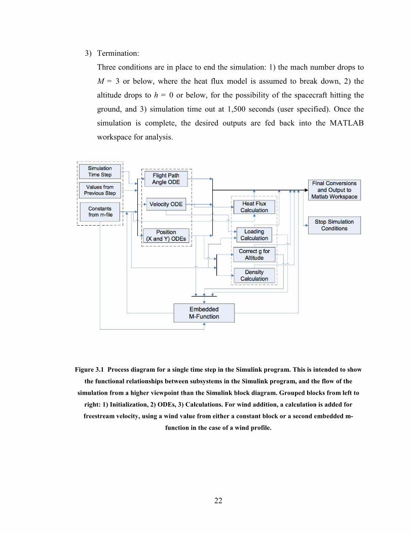
3) Termination:

Three conditions are in place to end the simulation: 1) the mach number drops to

M = 3 or below, where the heat flux model is assumed to break down, 2) the

altitude drops to h = 0 or below, for the possibility of the spacecraft hitting the

ground, and 3) simulation time out at 1,500 seconds (user specified). Once the

simulation is complete, the desired outputs are fed back into the MATLAB

workspace for analysis.

Figure 3.1 Process diagram for a single time step in the Simulink program. This is intended to show

the functional relationships between subsystems in the Simulink program, and the flow of the

simulation from a higher viewpoint than the Simulink block diagram. Grouped blocks from left to

right: 1) Initialization, 2) ODEs, 3) Calculations. For wind addition, a calculation is added for

freestream velocity, using a wind value from either a constant block or a second embedded m-

function in the case of a wind profile.

23

3.3 Simulation Accuracy

The physical model must be well understood before its results can be validated as

realistic—especially for models using differential equations, as integrator blocks may

hide errors in the model by smoothing their outputs [15]. To test the physical model,

simulation results will be compared with data from the re-entry of the Apollo 4 spacecraft

in Section 3.6.

Beyond the physical model, optimum simulation accuracy is achieved by

choosing an appropriate step-size and ODE solver. A smaller step size will give more

accurate results, but at the cost of computational effort. Comparing the simulation results

with data from Apollo 4 will help in determining this, as well as finding an appropriate

step solver to use out of the many choices Simulink offers—which is a process that

contains its own trade-offs.

3.4 Step-Solver Study

There are many step solvers to choose from in Simulink, each with its own

advantages and disadvantages. The best way to choose a step solver is by

experimentation. There are two types of solvers available, fixed and variable. Variable

step solvers change the step size depending on the rate of change of the model states,

allowing for less computation and faster simulation run times, but at the cost of loosing

some information. Fixed step solvers keep the same step size throughout the simulation.

Because information about the entire re-entry trajectory was desired for this study, using

a fixed step solver was determined to be the way to go.

All of the fixed, continuous solvers were tested using the final set of parameters

derived from the results of Sections 3.7 and 3.8 (the default fixed-step solver ODE3 was

used to generate results for these sections). The purpose of testing the other solvers was

to see if any added efficiency could be gained without loosing accuracy, i.e. if using a

different solver would allow faster computation times. Results showed that most solvers

24

performed similar to or worse than ODE3 in computation times and generated similar

results, with the final range of each trajectory being close to the one generated by ODE3.

Thus, it was decided that ODE3 should still be the solver to use for the simulations.

3.5 Apollo 4 Case Study

To confirm the validity of the model, simulation and optimization programs,

reconstructed data from the flight of Apollo 4 will be used. The data used for comparison

with the simulations in this study has been taken directly off of graphs from [14] and [16]

available for download on the NASA History Division website. The NASA History

Division did not provide raw data points from the flight, but considering the simulation

model is already based upon many simplifying assumptions, a reconstruction of the data

from these documents will suffice.

The first Apollo spacecraft to be launched atop the behemoth Saturn V rocket on

November 9th

, 1967, Apollo 4 (also known as AS-501) was an unmanned test of the

Apollo space capsule designed to bring astronauts to the moon, and the first to return the

spacecraft to Earth at a lunar return velocity. One of the main objectives of the flight was

to test the performance of the heat shield at lunar re-entry velocities, making it a good

source of re-entry heating data in addition to guidance and control information.

While the spacecraft entered at a lunar return velocity, it was not flown to the

moon. The engines of the Saturn V and its component boosters were burned in such a

way as to produce a trajectory that would bring it back to Earth at lunar return speed.

Approximately 8 hours after being launched, Apollo 4 splashed down northwest of

Hawaii at 172.52°W and 30.10°N, approximately 10 nautical miles from the target

splashdown point [17]. Fig. 3.2 is a photo of the recovered capsule from [14].

25

Figure 3.2 The Apollo 4 Command Module CM-017 being hoisted above its recovery ship, the U.S.S.

Bennington [14]. The capsule is currently on display at NASA’s Stennis Space Center in Bay St.

Louis, Mississippi.

While it is currently uncertain as to which vehicle the United States will use in the

near future to get humans to low Earth orbit, be it the Orion capsule from Lockheed, the

Dragon capsule from SpaceX, or a spacecraft from another company, one thing is certain:

the space shuttle will be retiring soon, and any future human-rated spacecraft in develop-

ment, at least in the near future, will be a capsule. These upcoming changes to the U.S.

space program underpin the value of using data from Apollo 4 for simulation validity in

Section 3.7. Table 3.1 lists parameters for the flight, which will be used as parameters for

the simulation.

26

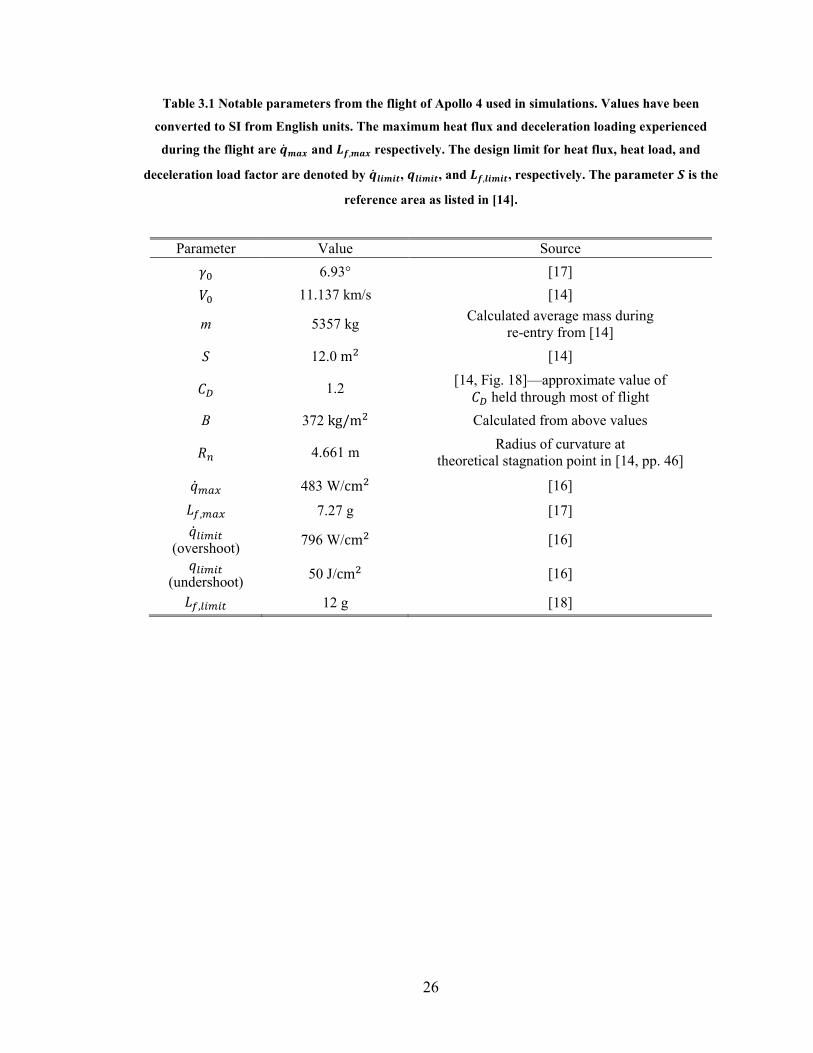
Table 3.1 Notable parameters from the flight of Apollo 4 used in simulations. Values have been

converted to SI from English units. The maximum heat flux and deceleration loading experienced

during the flight are �� ��� and ��,��� respectively. The design limit for heat flux, heat load, and deceleration load factor are denoted by �� �����, ������, and ��,�����, respectively. The parameter � is the

reference area as listed in [14].

Parameter Value Source

�= 6.93° [17]

�= 11.137 km/s [14]

m 5357 kg Calculated average mass during

re-entry from [14]

� 12.0 m% [14]

/0 1.2 [14, Fig. 18]—approximate value of /0 held through most of flight

B 372 kg/m% Calculated from above values

Mc 4.661 m Radius of curvature at

theoretical stagnation point in [14, pp. 46]

R�+P� 483 W/cm% [16]

U,+P� 7.27 g [17]

R���+�] (overshoot)

796 W/cm% [16]

R��+�] (undershoot)

50 J/cm% [16]

U,��+�] 12 g [18]

27

3.6 Correction of Stagnation Point Heating Constant

The exact point at which maximum heat flux occurs in the re-entry of Apollo 4, or

clues as to how to find it, are not listed in any of the sources used in this chapter.

However, it was found that for simulated trajectories close to that of Apollo 4, the

maximum value of heat flux always occurs in the initial entry phase of the flight—i.e.

before or during the first local altitude minimum in the trajectory.

To adjust the constant C in Eq. (2.13) such that the maximum heat flux of a

trajectory matched that of Apollo 4, a value of U/} was found such that the first local

minimum of the simulated flight path matched that of the reconstructed flight path of

Apollo 4. Using the value of C from [12] and a constant U/} � 0.52 in the simulation,

the location of peak heating was found at a range of 773.9 km, just before the local

altitude minimum at around 800 km. The heat flux at this point was less than half of that

experienced during Apollo 4—thus the constant from [12] is too low. The velocity and

density were found at the location of peak heating to be 10.38 km/s and 4.035 E-4

kg/m�, respectively, and were put back into Eq. (2.13) along with the maximum heat

flux experienced during Apollo 4 of 483 W/cm%, to solve for a new value of C. This

value was calculated to be C = 4.642 E-4 ��� �3 �@�, and will be used in all further

simulations.

3.7 Comparison of Results with Apollo 4 Flight Data

In order to prove that the results being generated by the simulation are valid, it

will be compared with the reconstructed flight data of Apollo 4 from [14]. First, the

control input is approximated to best match the vertical U/} from [14] as shown in

Figure 3.3. During the flight of Apollo 4 in the initial phase of re-entry, the guidance

program directed the vertical lift vector down for approximately 22 s to prevent skip out.

As shown in Fig. 3.3, this was a very rapid, short duration change, and was critical to

keeping the spacecraft along the desired trajectory. Thus, to approximate the control

28

input, the vertical U/} plot in Fig. 3.3 was split into 30 s intervals to capture the critical

point, and the average between the highest and lowest values of U/} for each interval

(read directly off of the plot) was taken to use as the control input values.

The control input in the simulation is defined by making an initial guess of the

final time, breaking the control input up into normalized time intervals, and allocating the

control inputs into their respective intervals. The elapsed time from entry interface to the

point in the trajectory where the spacecraft’s velocity dropped to O � 3 was 585 s, thus

the control input was split into 19 total intervals of 30 s duration. After running a

simulation using the approximate control input, the final time was adjusted so that the

final range of the simulation matched that of the final range of Apollo 4 when it reached

O � 3. Through this process it was found that an increase in simulation accuracy was

needed, thus the step size was decreased to 0.1 s so that the final range of the trajectory

could come within 1% of the final range of Apollo 4. The optimum final time for this was

589.9 s. Fig. 3.4 shows how the control input was applied with respect to simulation

time. More information on the numerical methods involved in control input definition can

be found in Chapter 5.

Final simulation results show that the trajectory generated from Apollo 4

parameters and approximate control input is a pretty close fit. The simulated trajectory

shown in Fig. 3.5 is slightly lower in altitude than Apollo 4, which may be due to 3-D

aspects not being included, mismatch in the atmospheric models used, and control input

approximation. As a result of the trajectory being lower in altitude, stagnation point heat

flux shown in Fig. 3.6 and deceleration loading shown in Fig. 3.7 are slightly higher, but

still within limits. The deceleration loading from the simulation is similar to the loading

that occurred during the flight of Apollo 4, as plotted in Fig. 3.8 from [14].

29

Figure 3.3 Apollo 4 vertical lift to drag ratio vs. ground elapsed time in seconds. This has been

deliberately modified from the original plot in [14] to end at ~30553 s, or the time at which Apollo 4

reached Mach 3 (585 s after entry interface).

Figure 3.4 Approximated control input using average values from [14] at 30 s intervals.

30

Figure 3.5 Simulated trajectory after applying the approximate Apollo 4 control input (solid line),

compared with the reconstructed trajectory of Apollo 4 from flight data (dotted line). The mismatch

in trajectories may be due to differences between the atmospheric models, and 3-D control aspects

not being included.

31

Figure 3.6 Stagnation point heat flux vs. horizontal range from the simulation. The maximum value

at 520 W/c�� is slightly higher than that of Apollo 4 at 483 W/c��, but this is to be expected as the simulated trajectory dips slightly lower in altitude from the flight path of Apollo 4 in the initial

altitude minimum.

32

Figure 3.7 Deceleration load factor vs. range for the simulation. The maximum value at 7.91 g, like

the heat flux, is slightly higher than that of Apollo 4 at 7.27 g. Again, this is to be expected, as the

simulated trajectory dips slightly lower in altitude from the flight path of Apollo 4 in the initial

altitude minimum.

33

Figure 3.8 Apollo 4 deceleration loading vs. ground elapsed time from [14], for comparison with

Figure 3.7. This plot covers the entire trajectory until guidance program termination.

34

3.8 Wind Addition

The effect of adding wind on a simulated trajectory based on the model laid out in

Chapter 2, and numerical methods to be described in Chapter 5, is discussed in this

section. First, a simulation was run with a constant tail wind of 30 m/s, and constant

control input of U/} � 0.22. Predicted results of adding a tail wind include an increase in

final range and a decrease in the maximum heat flux and deceleration loading that results

from the lower velocity of the spacecraft with respect to air (or the freestream). Results of

the trajectory comparison shown in Figure 3.9 between calm and constant 30 m/s wind

agree with these predictions. However, it was also expected that the final range offset

would be small, comparable to the zero-angle of attack results presented in [12], yet

results show a large extension in final range. There may be many factors that contribute

to this, perhaps the added kinetic energy just continues to build throughout the trajectory,

in turn sending it higher upon the second maximum in the trajectory where drag forces

are lower, thus allowing even more velocity to be retained.

Figure 3.9 Simulated trajectories at constant L/D for calm (dotted line) and constant wind conditions.

35

In order to better simulate actual atmospheric conditions, the HWM93 horizontal

wind profile [19] is used for the location and time of year of the Apollo 4 splashdown

from [17]. Fig. 3.10 shows a plot of this profile, which only extends up to 75 km. Wind

velocities above 75 km are assumed to be zero, based on the fact that the air density

beyond this altitude is extremely low anyway, and thus wind will have little effect on the

trajectory.

Figure 3.10 Plot of horizontal wind velocity from the HWM93 wind model at the location and time of

year of the Apollo 4 splashdown. Positive wind velocities are in the East direction.

A similar comparison was made between calm and profile wind trajectories as in

the constant wind case. Results plotted in Fig. 3.11 show that the wind profile pushes the

trajectory slightly less east than the constant 30 m/s wind did.

36

Figure 3.11 Simulated trajectories at constant L/D for calm (dotted line) and wind profile conditions.

In a final test, the wind profile is added to the Apollo 4 simulation from Section

3.7. Now with an approximated control input, appropriate parameters, and wind profile

matching the splashdown location and conditions, the simulation that should be closest

yet to matching conditions from Apollo 4 is plotted in Fig. 3.12. The final time value

used for defining the control input was once again adjusted to match the simulation final

range with the Apollo 4 final range, and was determined to be 585.0 s. There doesn’t

appear to be much difference between the calm and wind profile trajectories, other than a

slight offset towards the east during the up-control and final phases of entry.

37

Figure 3.12 Simulated trajectory (dotted line) using Apollo 4 approximate control input and wind

profile, compared with the reconstructed flight trajectory of Apollo 4. The addition of the wind

profile doesn’t seem to perturb the trajectory by much from Fig. 3.5—only moving slightly up-range.

38

Chapter 4: Problem Formulation

4.1 Problem Definition and Description

This thesis focuses on the mission objective of minimizing the distance between a

specified target range and the final range of the trajectory (as defined by the simulation

stop conditions listed in Chapter 3, i.e. � � 0, and O � 3). The control to be optimized in

accomplishing this is the lift-to-drag ratio, U/}. A change in U/} during re-entry is made

by adjusting the spacecraft’s angle of attack with a Reaction Control System (RCS). It is

desirable to correct the trajectory as little as possible to conserve fuel for the RCS, thus a

minimum amount of control input is also desired.

Safety constraints, based upon the design limitations of the spacecraft and the

ability of its payload to withstand the intense heat and deceleration loading produced by

re-entry, must also be considered. Increasing the lift on the vehicle may be a means of

reducing the amount of heating and loading, but too much lift will cause the spacecraft to

skip out of the atmosphere. This imposes an additional constraint on the trajectory. A

“skip-out” trajectory will be defined here as a trajectory with an altitude greater than a

specified value ���+�]. In summary, the constraints imposed on the trajectory are:

U � U,��+�] , (4.1)

R� � R���+�] , (4.2)

and

� � ���+�] . (4.3)

In addition to the challenges listed so far, uncertainties in the re-entry trajectory,

generated by multiple sources, must be taken into consideration and minimized. Robust

39

trajectory planning as a means of dealing with these uncertainties will be discussed in

Chapter 7, but not studied or tested for in this thesis.

4.2 Application of Parameter Optimal Control to Re-entry

The advantages of using parameter optimal control are twofold: 1) it is easier to

solve for numerically, and 2) it fits the real-world situation better, as applying control

input in short bursts when needed is desired anyway, as opposed to continuously applying

control input knowing a control history ���� to follow from a general optimal control

solution. A generic parameter optimal control algorithm as described in [20] will be

applied to the re-entry model described in Chapters 2 and 3 to satisfy the mission

objective. The numerical implementation of this algorithm will be described in Chapter 5.

We will start by laying out the parameters defining the control input, then lay out

the algorithm. The control input is broken up into n normalized time intervals, �, such

that

�� � �c ��cP�, (4.4)

where k is an integer with values inside 1 � � � �, and ��cP� is the total time it takes for

the trajectory to be flown. This can also be expressed in vector form, and will be referred

to here as the � d 1 interval vector,

� � y�T �% � ��cP�z�. (4.5)

The control inputs for each interval make up the � d 1 control vector,

�� � y�T �% � �cz�. (4.6)

We then wish to minimize the distance from the target range, i.e. the scalar cost,

40

� � 1���� ! �]P\5^]4%. (4.7)

Three initial guesses must be made so that the partial derivatives of the cost

function with respect to each control input can be calculated: 1) an initial guess for the

optimum control input that achieves the target final range �]P\5^] (call this the initial

control input ��=), 2) an initial guess of the final time of the simulation to define the inter-

vals of control input, and 3) an initial parameter update, aimed at minimizing the cost

function after the first simulation has been run with the first set of inputs.

The partial derivatives of the cost function with respect to the control input for

each interval are required to generate a parameter update, thus prompting the need for an

� d 1 initial parameter update vector ∆��T. The first update of the control vector,

��T � ��= ' ∆��T, (4.8)

is used to compute the partial derivatives contained by the � d 1 derivative vector,

����� � � ������

��$��$ � ��b

��b � . (4.9)

Note each cost function is specific to its interval and will not be the same value as the

cost function used to determine optimality (i.e. from a simulation run with all inputs

updated). Further details on how this derivative is computed are laid out in Chapter 5.

All further parameter updates are computed from the derivative vector, where the

expression for the update is:

���IT � ��� ! ¡ ������ , (4.10)

where i is the current iteration and ¡ ¢ 0 is a step size. This process is repeated until the

control input is optimized, with the previous final time used as the final time guess for the

next iteration. The idea behind this is that if a small enough step size is used, the

difference in final time from one loop iteration to the next is negligible—ideally,

41

infinitesimally small such that Δ� ¤ 0. Then the value of � from the previous iteration

can be assumed to define the normalized time intervals of the current iteration.

A solution is achieved if either of two conditions are satisfied: 1) the cost function

I drops below a value �+�c determined by the user to be low enough to be considered an

optimum solution, or 2) the number of iterations i of the algorithm equal ¦+P�, also

determined by the user based upon what is considered optimal.

4.3 Optimization Study

After validating that the algorithm is implemented correctly, the goal is to observe

the behavior of the parameter optimal control algorithm when applied to the problem

stated in Section 4.1, to draw some conclusions as to how effective a solution the

algorithm is, and to identify areas worthy of further research and development towards

use of the algorithm as an approach to trajectory planning and real-time optimization. The

subsections to follow outline the tests to be completed in the study, purpose for each, and

predicted results. Test parameters, methods used, and results of each test will be listed in

the respective sections of Chapter 6.

4.3.1 Validation

Before the algorithm can be studied it must first be confirmed to work properly

and generate valid results. If it is optimizing the control input, the expected result will be

the cost function decreasing smoothly with each iteration of the loop until it reaches

either of the user-defined conditions for an optimal solution. For multiple intervals

(� ¢ 1), each control input value should be optimized independently of the other values,

e.g. if the initial guess for the control input has the same value for each interval, and the

values are not optimized independently, then upon completion of the program, all

optimized values would be the same—as if there was only one interval used, � � 1.

42

4.3.2 Program Robustness

If the program is robust, it should be able to optimize the trajectory regardless of

the initial guess for control input, initial step, or final time. The cost function should

decrease regardless if the initial guess is above or below the optimum value, i.e. the initial

trajectory overshoots or undershoots the target range. If the final time is far off from the

actual final time of the simulation, the program should be able to correct for it. There may

be limits to the program’s ability to compensate for a far off initial guess—these limits

should be identified as a measure of how robust the program is. In addition to the initial

guess parameters, the program should be able to optimize despite changes in other control

parameters as well, such as the target range or step size.

4.3.3 Effects of Wind Addition and Increasing the Number of Intervals

These tests attempt to gain insight into the behavior of the program when an

increased amount of complexity is added by addressing the following questions:

• What happens if wind is present in the re-entry model?

• What happens as the number of intervals n is increased?

• Are there any benefits to increasing the number of intervals?

• What is the computational cost of increasing n?

• Is there a limit to how much n can be increased? If so, what is this limit and what

causes it?

With the above questions in mind, the following predictions are made:

1. With wind added, it should take more effort to reach a solution.

2. As n increases, computational cost will increase, ability to minimize the cost

function will increase, and step size needed should decrease in order to handle the

added complexity.

43

3. The program should be able to solve for any number of intervals used.

Figure 4.1 illustrates the predicted results.

Figure 4.1 Predicted results for increasing n.

4.3.4 Constraint addition

If constraints are added successfully, the program should be able to find an

optimal trajectory that satisfies the constraints. It should be able to correct for constraint

violations when they occur during optimization, and ideally, also be able to correct an

initial guess that violates constraints before proceeding with optimization. Increasing the

number of intervals should allow more flexibility in the solution, and allow the program

to more precisely adjust the control input. Evidence of the possible need for this is the

sudden change in the lift vector from positive to negative for 22 seconds near the

beginning of the trajectory for Apollo 4, determined by the guidance control system to be

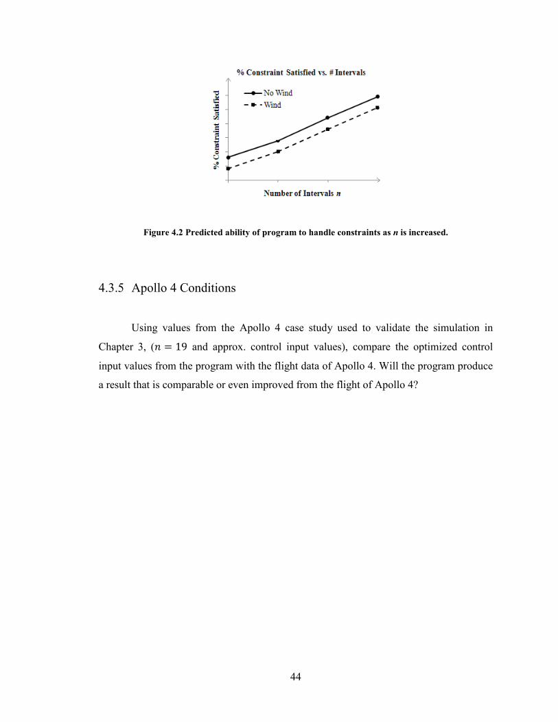
necessary to prevent skip-out. Figure 4.2 illustrates the predicted results, assuming that

even if the program is unable to fully satisfy the constraint, it should at least be able to

partially satisfy it. Another way this potential benefit could be shown is if the program

takes less iteration (and therefore less run time) to solve for the optimal solution, or is

able to drive the cost function lower with the added precision of more intervals.

44

Figure 4.2 Predicted ability of program to handle constraints as n is increased.

4.3.5 Apollo 4 Conditions

Using values from the Apollo 4 case study used to validate the simulation in

Chapter 3, (� � 19 and approx. control input values), compare the optimized control

input values from the program with the flight data of Apollo 4. Will the program produce

a result that is comparable or even improved from the flight of Apollo 4?

45

Chapter 5: Numerical Methods

5.1 Control Input and Constraint Information via Simulink

The “interval” embedded m-function collects constraint information and chooses

the control input to use based on the current time interval. For the control input at a given

time step, once the current time interval is identified, the value of U/} corresponding to

that interval is picked out of the control vector and used as the input at that time step. If

the simulation time surpasses the final time guess � specified by the user, the control

input is reset to the value in the first interval, � � 1. This avoids discontinuities in the

control input.

If a constraint is violated during the time step, the element of the � d 1 constraint

vector corresponding to the current interval is updated with the type of violation that

occurs (heating, loading, altitude, or combination of the three). The constraint vectors

from each time step in the simulation are assembled into an � d © constraint matrix that is

fed into the MATLAB workspace for use in the optimization loop. This information is

then used to stop a normal update to the input if it violates a constraint, or in the case of

the first run of the simulation, to exit the program altogether and ask for a different initial

guess. Figure 5.1 shows the embedded m-function block within the Simulink model.

46

Figure 5.1 “Interval” embedded m-function block within the Simulink model. Inputs are on the left

and outputs on the right.

5.2 Algorithm Implementation

The MATLAB code used to implement the parameter optimal control algorithm

in Chapter 4 can be found in Appendix E. This will optimize the control input for a 2D

re-entry trajectory given the required parameters.

The first iteration of the algorithm is performed outside of the optimization loop

itself. This uses the user-specified optimization parameters, initial guess, and constraints

to simulate the first trajectory, compute the initial value of the cost function, and check

for constraint violations. If statements are used to exit the program at this point if any of

the constraints are violated, prompting the user to try another initial guess. Otherwise, the

control vector is updated with the initial parameter update ∆��T, the interval vector � is

updated based on the final time of the first simulation, and other results are passed into

the optimization loop for use in further computation.

A for loop is used to carry out the optimization algorithm after the first run

through. First, a simulation is run using the updated control vector computed from the

previous iteration as input. Constraint information is obtained from this simulation, along

with an updated cost function and interval vector. If the cost function drops below the

user specified value �+�c, or if the number of loop iterations i is equal to the user

47

specified value ¦+P�, the values in the control vector will be considered optimum and the

loop will terminate.

A nested for loop is used to carry out the partial derivative calculations and

parameter update for each interval. For an interval n, a simulation is run to find the effect

of its parameter update from the previous iteration, �c,�, on the current cost function ��. This is done by allowing only one interval’s control input to be the updated value in the

control vector, while holding all other inputs to their pre-update values. For example, if

we split the control input into four intervals, and we are seeking a parameter update for

the second interval, the input vector would be:

�� � y�T,�@T �%,� ��,�@T �f,�@Tz� . (5.1)

The partial derivative is then,

? ���ªCc,� � �b,«@�«¬�

ªb,«@ªb,«¬� (5.2)

where �c,� is the cost function resulting from the control input in Eq. (5.1), and ? ���ªCc,� is

the partial derivative for interval n in the current iteration of the loop. The full partial

derivative vector ����� is then constructed from the partial derivatives calculated for each

interval, and then used in Eq. (4.8) for the parameter update. Once the entire control

vector has been updated, the loop is complete, and the updated vector is used as input for

the simulation in the next iteration.

5.3 Wind Addition

To add horizontal wind to the simulation, a calculation is added to the Simulink

model for freestream velocity, as well as a modified update to the absolute acceleration

equation and flight path angle equation. All that is needed to include a constant wind in

48

these updates is a “constant” block. For a wind profile, a second embedded m-function is

added. In a similar manner as the “interval” m-function, the “hwindv” function shown in

Fig. 5.2 outputs the value of horizontal wind from an array of wind velocities generated

by the HWM93 wind profile that corresponds to the current km of altitude.

Figure 5.2 “hwindv” embedded m-function block within the Simulink model. Inputs are on the left

and outputs on the right.

Notes on Simulink implementation:

• Array of wind velocities from the wind profile read in from a text file.

• Velocity update follows integrator block in acceleration equation.

• Flight Path Angle (FPA) update follows FPA integrator block in FP angular

velocity equation.

• Freestream velocity replaces the absolute velocity when fed into acceleration, heat

flux and dynamic pressure equations.

• For loading, a derivative block is used to find the freestream acceleration,

replacing the absolute acceleration fed into this calculation.

49

Chapter 6: Results

6.1 Summary

This chapter describes the methods and results of each test that was laid out in

Chapter 4. Results show that implementation of the optimization loop was successful up

to a certain point, and that a different approach is required if constraints are to be applied

successfully with this parameter optimal control algorithm. Conclusions drawn from

these results are discussed in Chapter 7. Tabulated results for the undershoot, overshoot,

and undershoot with wind profile cases used in this study are included in Appendix D.

6.1.1 Test Parameters

The same optimization parameter values as listed in Table 6.1 are used for each

test unless otherwise noted. Specifications for the computer hardware and software used

for conducting the tests are in Table 6.2.

50

Table 6.1 Baseline or “undershoot” test parameters. Limits on heating, loading, and altitude apply

only to the constrained tests. The ­ d � superscript indicates that the value is the same for all elements of the vector. No wind is present in the baseline case.

Parameter Value

¡ 10@TT

∆��T y0.001zcdT

��= y0.2zcdT

� (initial) 589.5 s

�]P\5^] 3797 km

�+�c 1

¦+P� 1000

R���+�] 700 W/cm%

U,��+�] 12 g

���+�] 121.9 km

Max Sim Time

Allowed 1500 s

Solver ode3 (Bogacki-

Shampine)

Sim Step Size 0.1 s

Table 6.2 Hardware and software specifications. X11 is required to run MATLAB in Mac OS® X,

and without it the embedded m-functions will not compile. Mac® and Mac OS are trademarks of

Apple Inc., registered in the U.S. and other countries. X11 © Copyright X.org Foundation.

Computer Used: 2009 MacBook® Pro 15”

Operating System Mac OS X 10.6.2

Processor: 2.66 GHz Intel® Core™ 2 Duo

Memory: 4 GB 1067 MHz DDR3

MATLAB Version Used: 7.9.0.529 (R2009b)

32-bit (maci)

August 12, 2009

Simulink Version Used: V7.4 (R2009b)

X11 Version Used: XQuartz 2.3.4 (xorg-server 1.4.2-

apple45)

51

6.2 Validation

First, the simplest possible case was tested—only one interval (� � 1), calm

winds, and no constraints applied. Figures 6.1 and 6.2 show a smooth decrease in the cost

function with loop iteration and final range, respectively, and Figure 6.3 shows a smooth

final time update as well. The optimized control inputs and trajectory are presented in

Figure 6.4 and 6.5, respectively. This shows a successful implementation of the algorithm

with smooth updates of the cost function and final time. The cost function was able to be

minimized to within the �+�c parameter, thus the final range of the optimized trajectory

was within 1 km of the target range. The optimum control input that achieved this was

U/} ¯ 0.225.

To show that the control input for each interval is optimized independently, the

same program configuration was run, but for � �1, 2, and 3. All results show inde-

pendent updates for the control input regardless of the number of intervals. For most

intervals, it appears the optimum control input values are close to 0.22. Figure 6.6 shows

the final control input for � � 3 intervals as an example of the results produced.

If the initial guess is very far off from the optimum value(s) for the control input,

the trajectory may skip out past entry interface altitude. When this happens, no updates

are made to the control input as a consequence of the lack of air density. In other words,

with no air, there is no lift or drag forces on the spacecraft, and thus changes to L/D have

no effect on the trajectory (i.e., the derivative ����� ¤ 0, thus the update ∆�� ¤ 0). With no

updates, the optimization process becomes unstable, and the cost function actually

increases until all intervals skip out. Once this occurs, the control values are stuck, and

the program must be terminated manually (CTRL + C). This reinforces the need to

implement an altitude constraint in the program.

52

Figure 6.1 Cost function progress vs. loop iteration for ­ � 1, baseline parameters.

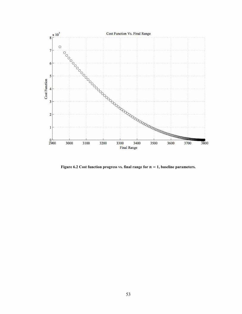
53

Figure 6.2 Cost function progress vs. final range for ­ � 1, baseline parameters.

54

Figure 6.3 Final time progress vs. loop iteration for ­ � 1, baseline parameters.

55

Figure 6.4 Optimized control input vs. time for ­ � 1, baseline parameters.

56

Figure 6.5 Optimized trajectory for ­ � 1, baseline parameters (solid line), compared with the trajectory of Apollo 4 as reconstructed in Chapter 3.

6.3 Program Robustness

To judge if the program was robust to different values of ��=, the program was run

using an initial guess of ��= � y0.24zcdT for � � 1, 2, and 3 intervals, and other param-

eters set to the same values as in the previous section. The value of ��= chosen is on the

“other side” of the optimum input from the initial guess used in Section 6.2, thus these

tests were intended to show that the program can optimize the trajectory in “both

directions.” All results demonstrated that the program could optimize the trajectory for an

initial guess that undershoots or overshoots the target range. Figures 6.6, 6.7, 6.8, and

6.9 show the final time update, cost function update, optimized trajectory and control

input, respectively for the single interval test.

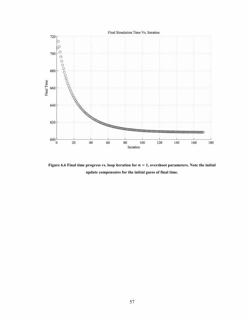
57

Figure 6.6 Final time progress vs. loop iteration for ­ � 1, overshoot parameters. Note the initial update compensates for the initial guess of final time.

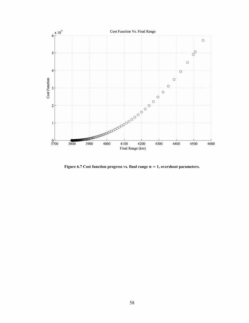
58

Figure 6.7 Cost function progress vs. final range ­ � 1, overshoot parameters.

59

Figure 6.8 Optimized trajectory for ­ � 1, overshoot parameters (solid line), compared with the trajectory of Apollo 4 as reconstructed in Chapter 3.

60

Figure 6.9 Optimized control input vs. time for ­ � 3, overshoot parameters (thin black line) compared with the baseline optimized control input for ­ � 3 (thick gray line).

Intuitively, one would expect the optimum values of U/} to be the same

regardless of the initial guess, but from Figure 6.9 we can observe that this is not the case.

While the optimized inputs for the first interval are close to being the same value, the

other intervals are closer to their initial guess values. This demonstrates the influence

each interval has over the trajectory—and that one interval is dominant over the others in

its influence. The same result can be observed with other initial guess values and number

of intervals used. This result also shows that the control input used at the beginning of the

trajectory has a large effect on how the remainder of the trajectory will play out—

matching up with conclusions drawn from observing the brief 22 s switch to negative

control input early in the trajectory of Apollo 4. Greater resolution in the control input

(i.e. greater values of n) may help to pinpoint the locations of greatest influence over the

input.

61

To show the programs response for a change in the initial guess for final time,

simulations were run using � � 3 and values of � equal to 10 s and 1000 s, with all other

parameters the same as listed in Table 6.1. A single interval was not used because as

noted in Chapter 5, the control input is reset to the value in the first interval after the time

reaches the guess for � —therefore even if the predicted final time was far below the

actual final time, it wouldn’t make a difference anyway because the control input would

stay the same. Results of these tests show that the final time was corrected for

immediately upon the first iteration of the optimization loop—thus the algorithm works

as intended in this respect.

To observe the program’s behavior due to a change in the initial step, two

simulations were run using � � 3 and baseline parameters, with the exception of the

initial step, set at 0.01 and 0.0001. Comparing results using these parameters to the

results using the baseline value of 0.001, it appears that increasing ∆��T will decrease the

simulation run time, as listed in Table 6.3. However, once the initial step is increased

beyond a certain point, there is a higher risk of the trajectory skipping out, either after the

first update or sometime during the simulation.

Table 6.3 Results of changing the initial step.

Initial Step Runtime # Iterations to solution

0.01 525 s 215

0.001 561 s 236

0.0001 567 s 237

It seems that from the beginning of the loop onward, the initial step has an effect on the

overall step size the optimization loop is taking in improving the cost function. Thus,

when choosing the control update step size ¡, or when considering the level of accuracy

needed in the control input updates, the initial step must also be taken into consideration

as a component of the control update.

A smaller step size value ¡ will allow more resolution in the optimization

process, which may be needed in satisfying constraints or in optimizing for a large

62

number of intervals, but if too small with cause the run time to be too slow, such that it

would take days or weeks to find a solution with the hardware and software configuration

used. There is also an additional risk of non-updates, due to very small derivatives being

multiplied by a very small step size. MATLAB can handle numbers as small as

2 d 10@�=±, but after many loop iterations, the update may be driven down small enough

such that it is equivalently zero.

Increasing the target range will allow the program to have more flexibility in

finding a solution. A target range of 5000 km was used in the initial development of the

program. Once the baseline parameters were put into the program, the program was much

more limited in the initial guesses that could be used without skip-out occurring.

For the unconstrained case, �+�c can be driven to very low values. The lowest

value attempted was 0.1, and the program optimized the trajectory within this parameter

successfully. It is reasonable to assume it could be driven even lower, but other factors,

such as using a large number of intervals or applying constraints may limit the value of

�+�c that is possible to achieve.

6.4 Effects of Wind Addition and Increasing the Number of Intervals

Chapter 3 showed the effect of constant wind and a wind profile on a single

trajectory. In this section, the HWM93 wind profile will be added to the simulation used

in the optimization loop, with all other parameters at their baseline values. In addition to

wind being added to the program, undershoot and overshoot values in the previous

sections are run from � � 1 up to as many intervals as the program can handle. This was

intended to determine if there was a limit to the number of intervals the program could

run, if the limit stayed the same for each scenario, what the potential cause(s) may be for

the limit, and what the cost, benefits, and behavior of the program were with an

increasing number of intervals.

With wind added, it was expected that the program would require more effort to

compute an optimal trajectory—this prediction turned out to be mostly correct. It appears

as though adding the wind profile to the baseline case decreases the number of intervals

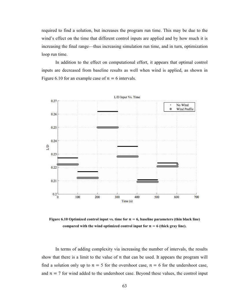
63

required to find a solution, but increases the program run time. This may be due to the

wind’s effect on the time that different control inputs are applied and by how much it is

increasing the final range—thus increasing simulation run time, and in turn, optimization

loop run time.

In addition to the effect on computational effort, it appears that optimal control

inputs are decreased from baseline results as well when wind is applied, as shown in

Figure 6.10 for an example case of � � 6 intervals.

Figure 6.10 Optimized control input vs. time for ­ � 6, baseline parameters (thin black line) compared with the wind optimized control input for ­ � 6 (thick gray line).

In terms of adding complexity via increasing the number of intervals, the results

show that there is a limit to the value of � that can be used. It appears the program will

find a solution only up to � � 5 for the overshoot case, � � 6 for the undershoot case,

and � � 7 for wind added to the undershoot case. Beyond these values, the control input

64

will be optimized and the cost function will decrease for a certain number of iterations,

until at some point a parameter update results in a trajectory that skips out past entry

interface altitude. In turn, further iterations only make the situation worse, with the skip

out occurring earlier in the trajectory with each iteration, until all intervals skip out and

no further parameter updates are made. This “skip-out instability” is similar to the one

that occurs for a bad initial guess, as noted in Section 6.2. The reason the wind case is

able to optimize using an additional interval may be due to the lower optimized control

input values that result when wind is applied, or perhaps a higher value of U/} is not

being applied until later in the trajectory—thus preventing skip-out.

The costs of increasing � are weighed in terms of the number of iterations and the

program run time it took to find an optimal trajectory. Figure 6.11 shows that for all three

scenarios, the number of iterations increased from one to two intervals, then slowly

decreased—thus showing a potential advantage to using more intervals. While the

program can optimize with seven intervals when wind is applied, clearly the results show

that it takes much more effort to solve for the optimum control input—a potential

precursor to instability in using larger values of n. For simulation run time, Figure 6.12

shows an increase in the simulation run time with increasing �, as expected in Figure 4.1.

This may be attributed to the derivative loop requiring an additional simulation run for

every interval added, in turn adding additional time to complete each iteration of the

optimization loop.

65

Figure 6.11 Computational cost in terms of the number of iterations required to find the optimal

control input.

Figure 6.12 Computation cost in terms of program run time to find the optimal control input.

150

200

250

300

350

1 2 3 4 5 6 7

Iterations i

Number of Intervals n

# Loop Iterations to Solution vs. # Intervals

Undershoot

Wind Profile

Overshoot

0

500

1000

1500

2000

2500

1 2 3 4 5 6 7

Run Time (s)

Number of Intervals n

Loop Run Time vs. # Intervals

Undershoot

Wind Profile

Overshoot

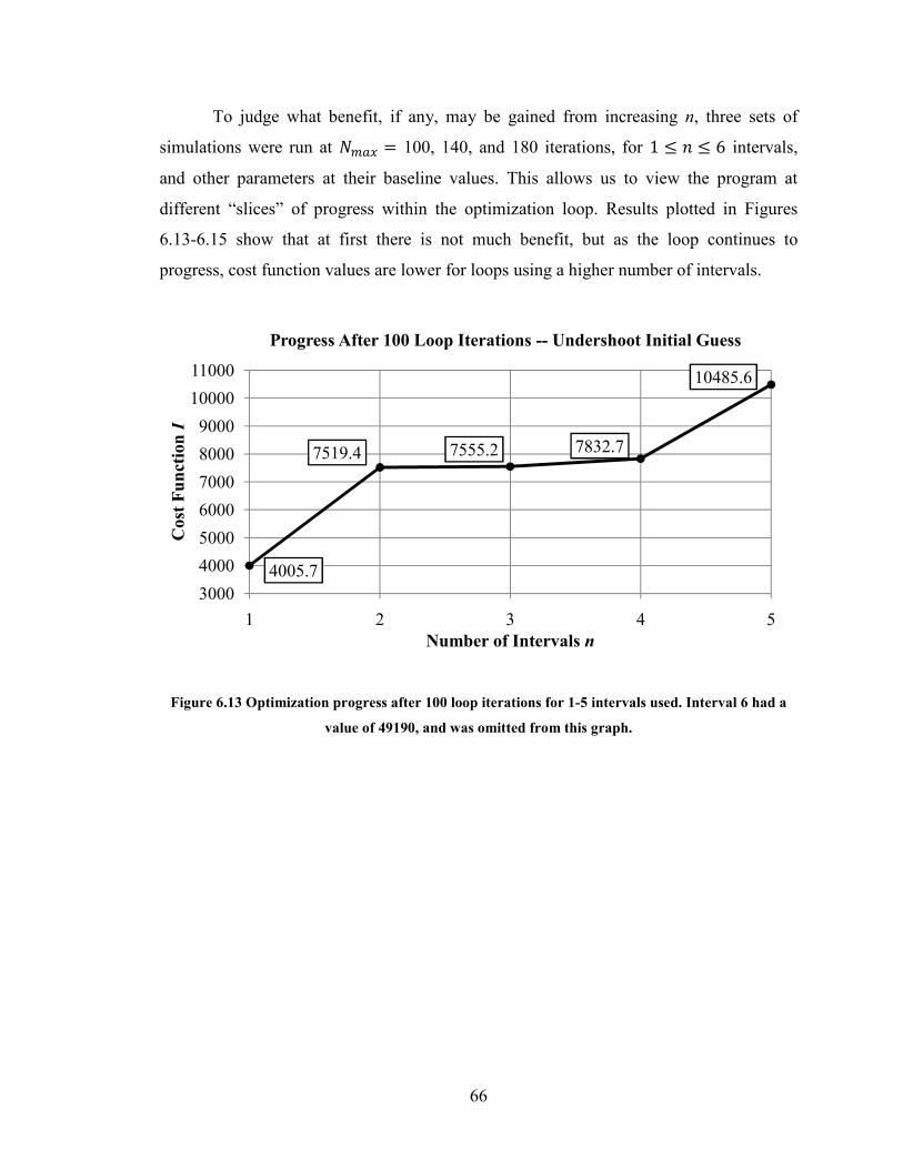
66

To judge what benefit, if any, may be gained from increasing n, three sets of

simulations were run at ¦+P� � 100, 140, and 180 iterations, for 1 � � � 6 intervals,

and other parameters at their baseline values. This allows us to view the program at

different “slices” of progress within the optimization loop. Results plotted in Figures

6.13-6.15 show that at first there is not much benefit, but as the loop continues to

progress, cost function values are lower for loops using a higher number of intervals.

Figure 6.13 Optimization progress after 100 loop iterations for 1-5 intervals used. Interval 6 had a

value of 49190, and was omitted from this graph.

4005.7

7519.4 7555.2 7832.7

10485.6

3000

4000

5000

6000

7000

8000

9000

10000

11000

1 2 3 4 5

Cost Function I

Number of Intervals n

Progress After 100 Loop Iterations -- Undershoot Initial Guess

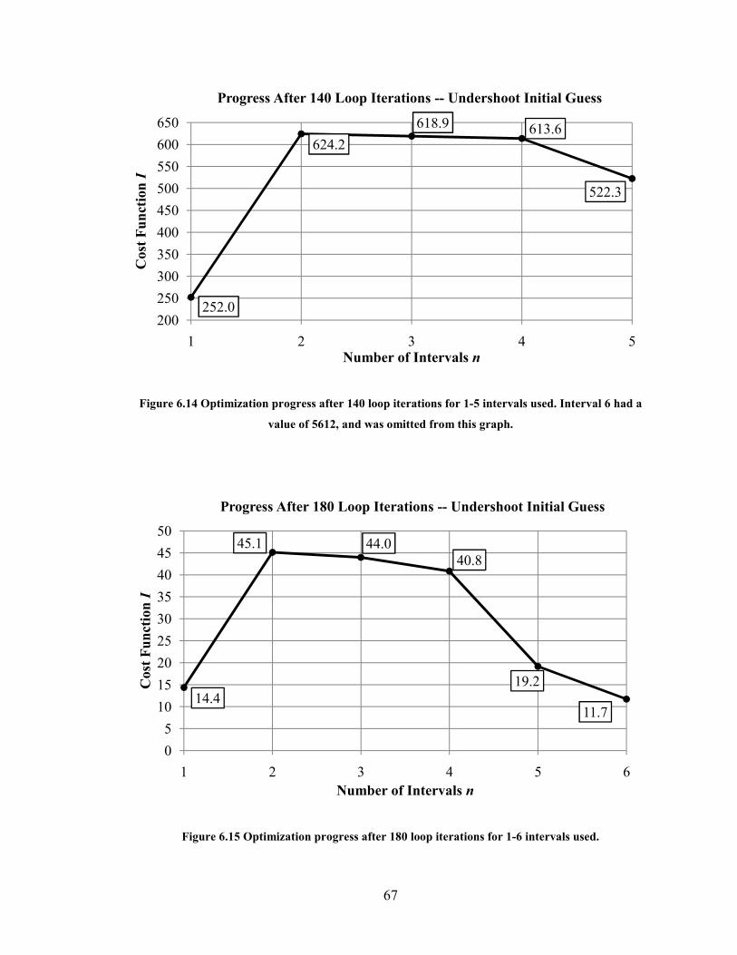
67

Figure 6.14 Optimization progress after 140 loop iterations for 1-5 intervals used. Interval 6 had a

value of 5612, and was omitted from this graph.

Figure 6.15 Optimization progress after 180 loop iterations for 1-6 intervals used.

252.0

624.2

618.9 613.6

522.3

200

250

300

350

400

450

500

550

600

650

1 2 3 4 5

Cost Function I

Number of Intervals n

Progress After 140 Loop Iterations -- Undershoot Initial Guess

14.4

45.1 44.0

40.8

19.2

11.7

0

5

10

15

20

25

30

35

40

45

50

1 2 3 4 5 6

Cost Function I

Number of Intervals n

Progress After 180 Loop Iterations -- Undershoot Initial Guess

68

In an attempt to show the direct effect of using different values of n on the

trajectory for the baseline case, trajectories from n = 2 through n = 6 are plotted on the

same graph in Figure 6.16. The trajectories are too close together to show much diff-

erence on this scale, so a zoomed in portion of the trajectory is plotted in Figure 6.17. The

overall trend is apparent with the trajectory going further inward as n increases.

Figure 6.16 Baseline trajectories from n = 2 through n = 6 plotted on the same graph, as well as the

Apollo 4 trajectory for comparison (faint dotted line). Obviously the trajectories are very close

together and not much detail can be shown. Figure 6.17 shows a zoomed-in portion of the graph

marked by the box.

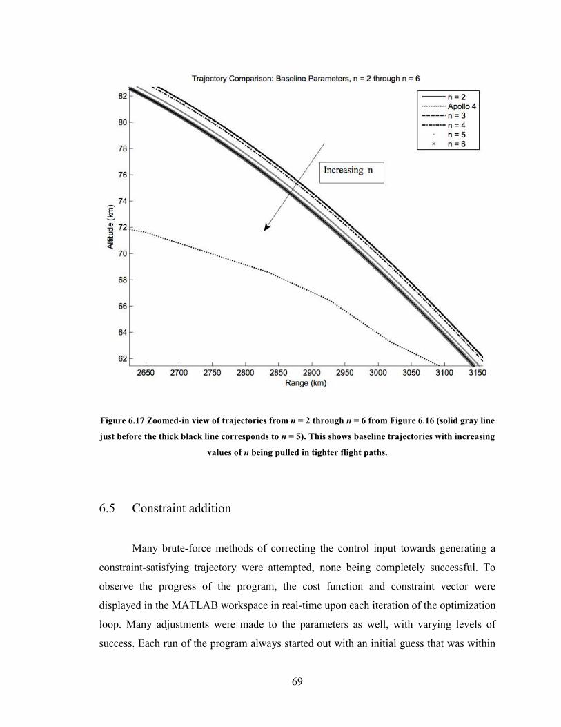
69

Figure 6.17 Zoomed-in view of trajectories from n = 2 through n = 6 from Figure 6.16 (solid gray line

just before the thick black line corresponds to n = 5). This shows baseline trajectories with increasing

values of n being pulled in tighter flight paths.

6.5 Constraint addition

Many brute-force methods of correcting the control input towards generating a

constraint-satisfying trajectory were attempted, none being completely successful. To

observe the progress of the program, the cost function and constraint vector were

displayed in the MATLAB workspace in real-time upon each iteration of the optimization

loop. Many adjustments were made to the parameters as well, with varying levels of

success. Each run of the program always started out with an initial guess that was within

70

the constraints, as the methods attempted to correct the initial guess before the loop was

executed also proved unsuccessful. Depending on the number of intervals used,

“ascending” or “descending” initial guesses for the control input vector (where the input

values increased or decreased with each successive element of the vector) were necessary

to initially satisfy the constraints. Typically constraints would then be violated in the next

iteration after the initial step was applied. This section lays out each method that was

attempted, and the behavior of the program that followed. Suggested methods to try next

in solving this problem are laid out in Chapter 7.

The first method attempted simply held the input of the constraint-violating

interval to that of its value before the violation occurred

��,�IT � ��,�@T , (6.1)

within the update loop, while allowing normal control input updates to the intervals that

did satisfy the constraints. Depending on the parameters used, this would at times allow

the algorithm to optimize-out the violations and then continue to update the inputs

normally, but eventually after a number of iterations a constraint violation would pop-up

in some other interval. Sometimes this would lead to a “yo-yo” effect, where the cost

function would jump back and fourth between two different values, sometimes with

improvement, sometimes with no updates to the control inputs such that the program had

to be terminated. A severe mismatch in the final time guess between loop iterations is the

most likely cause of this. Near skip-out trajectories have very long final times while

overly-steep trajectories have very short final times, thus a mismatch between the desired

and actual control input due to the final time guess is likely. Eventually, all cases lead to

a skip-out instability.

Many times the program would yo-yo back and fourth between violating the

heating and loading constraints (or both), and violating the altitude constraint. The

altitude constraint was taken out to judge if the program could handle just improving the

heating and loading constraints, but this also proved ineffective, as the program could

successfully weed out violations in an interval when they occurred, only to have them

pop up in other intervals, not unlike the “Wacky Gator” arcade game where the player

71

has to hit an alligator with a mallet when it pops out of its hole, only to have other

alligators pop out of the other holes and have to hit them too.

There are two places in the trajectory where heating and loading violations are

likely to occur—during the initial phase before the spacecraft begins to ascend again

(a.k.a. the “up-control” phase in Apollo), and during the final phase of entry when the

spacecraft is making its final descent to the ground. Thus it is possible for constraint

violations to be satisfied in one phase of the trajectory only to be violated in the other

phase. Sometimes the program was able to satisfy the constraints and reduce the cost

function normally for a few iterations, but somehow violations would slip in again, the

control inputs and cost function would jump around, and it would be back to square one.

This behavior would continue until © � ¦+P�, therefore yielding no useful solution.

Relaxing the constraints to allow higher values of heating, loading, and altitude yielded

similar results.

Going further approaching altitude, heating and loading constraints differently, a

different update was attempted, adding a constant to the control input of an interval that

violated the heating or loading constraints

��,�IT � ��,� ' Constant, (6.2)

and subtracting by a constant for an altitude constraint

��,�IT � ��,� ! Constant, (6.3)

where many different values for the constant were tried, from 0.001 to as high as 10. This

worked a little better in eliminating the constraints, the only downfall being that

sometimes the normal update of control input for certain intervals would blow up to huge

values, obviously violating constraints in the process. Because the constants used were

small in comparison to these input values, this method would do little to improve the

constraint from one loop iteration to the next. Making the constant very large only made

the situation worse. Many of the unstable behaviors noted for the previous approach were

also observed.

72

Attempting to make up for large updates when they occurred, a proportional

response to violations was attempted. Based upon “cost functions” of the constraint

values and the maximum values that occur in the constraint-violating trajectory

´T � �R�+P� ! R���+�]�% (6.4)

´% � 1U,+P� ! U,��+�]4% (6.5)

´� � �E+P� ! E��+�]�% , (6.6)

where the update will then be determined by the type of constraint that occurs

��,�IT � ��,� ' ´T�Constant� (6.7)

��,�IT � ��,� ' ´%�Constant� (6.8)

��,�IT � ��,� ! ´��Constant�. (6.9)

This involved adding a lot of additional complexity to the program in terms of logic

statements. Again, many different values for the constants were attempted, with results

similar to the previous results of applying just adding or subtracting a constant. There

seems to be just too much variation between these types of updates for fixing a constraint

violation and normal updates for optimization.

The results of these tests also show that the control input for the interval

immediately preceding the interval in which a constraint violation occurs also plays a role

in satisfying the constraints. For this reason, additional updates were included for these

intervals. While this was still ultimately unsuccessful, results show that this did help to

improve the constraints much faster than simply updating the control input for the

violating interval.

Going further in complexity with the constraint cost functions, another approach I

attempted to formulate was to pause the loop when a violation occurred and use a nested

73

optimization loop using the same algorithm to minimize the constraint cost function. This

would have added an immense amount of complexity to the program, especially

considering the partial derivatives of the constraint cost with respect to each interval’s

update would have been zero in most cases. It is my assertion from these results that

brute force methods will not work, and a different approach to these constraints is needed

before moving forward.

6.6 Apollo 4 Conditions

To see how the optimized input from the program would compare with the control

input of Apollo 4, and attempt was made to run the program with � � 19 intervals, and

an initial guess for the control input as listed in the case study of Chapter 3. Without

constraints working, this attempt was unsuccessful. If the step size ¡ was too large, a

skip-out instability would occur. For smaller values, the cost function did minimize

smoothly without violating constraints, but at a very slow rate, such that it would take

days or weeks for the program to finally compute a solution if allowed to run. Different

initial step values were used as well, but still did not ultimately yield better results.

Again, this highlights the need for constraints to be applied successfully for any practical

use of this optimization method.

74

Chapter 7: Conclusions

7.1 Summary

In summary, the results generated by the re-entry simulation have been

successfully validated, along with the optimization program up to a point. Constraints

will need to be added successfully for any further development of the algorithm. The

remaining sections of this chapter lay out areas of potential further research.

7.2 Simulation and Optimization Program Development

There are basically two directions to go in improving the program: adding

constraints successfully and increasing program efficiency. The next step in attempting to

add constraints to the program would be to first go back to what was used in the previous

optimal control algorithms for re-entry, such as [2] or other references listed in Chapter 1.

While these methods might not exactly fit with the parameter optimal control algorithm,

they may be a good place to start in developing new ideas and approaches towards

applying constraints.

There are also two other ideas were not formulated or implemented in Chapter 6

that may work—indirectly constraining the trajectory by applying constraints to other

parameters, and using a penalty function. Because the constraints don’t just depend on

U/} but also on many other parameters, such as freestream velocity, it may be more

effective to directly constrain the velocity instead of U/}. Applying a summation or

integral penalty function to heat flux for example

µ��� � ¶ ·R� · ¹�R� ! R�+P�� º�, (7.1)

75

where · is a weight and ¹ is a step function, may also be worth trying out. A quick

search online will yield many references on penalty functions. No matter what methods

are tried next, it is advisable to work on implementing only one type of constraint at a

time, then once they are working individually, try applying more than one constraint to

the trajectory. The brute force methods mentioned in Chapter 6 may not have ultimately

worked, but the benefit of approaching each constraint on a case-by-case basis was clear.

As far as improving the speed of the program towards computing fast enough to

be used in real-time, there are many paths to pursue. The most obvious would be to

simply use a faster computer set-up, but finding a more efficient way run the algorithm

will probably be a cheaper means of increasing speed. From the perspective of the

Simulink model, an increase in step size (assuming the accuracy loss is insignificant), or

the use of a variable step solver (assuming only the end state is needed and loosing

information about the trajectory is inconsequential) will certainly make each simulation

take less time to run. Considering the model has been validated as accurate, a variable

step solver might be the way to go—as long it is tested first. Using a different method

other than Simulink altogether, such as the ODE23 function in MATLAB, or even a

completely different programming language, may also be something to try.

Simulating real-time updates is also something that could be developed by

modifying the current program. All that would be needed is to pause or stop the

simulation at a desired point during entry, run the optimization loop, then use the values

of the state variables at that point as the initial values for the states in the next simulation.

In terms of run-time speeds, only the first run of the program will be the longest, then as

updates come in, simulations will take less time to compute, and run times will be

increasingly fast as the trajectory goes on. In addition, considering the “dominant

interval” results of Chapter 6, it may only be necessary to optimize for several control

inputs at the beginning of the trajectory, then use fewer and fewer intervals as the

trajectory progresses. In other words, the initial phase of the trajectory may require more

intervals of input at critical points (e.g. the 22 second negative input to keep Apollo 4

from skipping out), while the rest of the trajectory might only require one interval. It

would be wise to study not only optimum input values, but also the optimum number of

76

intervals to use in a given situation, and the optimum placement of these intervals. Less is

more when it comes to program efficiency—the less the program has to do, the better.

A few other ideas that may be worth pursuing in further development and testing

of the algorithm:

• Add a vertical component of wind, and account for its effects.

• Use different models for stagnation point heat flux, based upon appropriate

boundary layer conditions (i.e. frozen or equilibrium), wall temperature assump-

tions, and surface catalytic properties (this might be required if attempting to

simulate a space shuttle entry).

• See how well the program, once working, can optimize the trajectory of Apollo 4

in comparison to the flight data. This would provide many insights into the

performance of the program.

• Instead of using piecewise-constant control input, use piecewise-linear,

piecewise-quadratic, piecewise-cubic, etc. Though this might defeat the use of

parameter optimal control to save RCS fuel, perhaps in certain instances a

different control input method works best.

• Add a transfer function to represent the control response of an RCS motor.

7.3 Additional Problem Formulations

In addition to the problem laid out in Section 4.1, there are many other possible

re-entry problems in which applying parameter optimal control is a potential solution.

These include:

• Minimizing the final vertical velocity, changing the cost function to � � »�� ». • Taking heat shield ablator mass loss into account, minimize the amount or rate of

mass loss, and thus implement a cost function of � � ¼� .

77

• Extending the model to 3-D, 6-DOF. In this case, an additional constraint could

be applied to the cross-range, or it may be desired to maximize the cross-range

distance. This would also add the horizontal component of U/} (varied by the

RCS changing the roll and sideslip angles) and initial azimuth as control variables

that could be optimized. Some equations on this are listed in [12, pp. 143].

• Minimize the amount of fuel consumption from the Reaction Control System.

This may involve many different parameters to optimize, including the length of

time the engine is burned, and identifying the optimal places along the trajectory

the burns should be made.

There are most likely other formulations in which the algorithm may be useful. The

following sections describe modifications and changes that could be made to the re-entry

environment itself.

7.4 Stochastic Re-entry

A true optimal trajectory must take into consideration all possible sources of

restrictions and challenge reality places on it—and in reality, uncertainties are always

present. During re-entry, descent and landing or splashdown, many uncertainties arise,

such as:

• Non-standard atmospheric conditions

• Aerodynamic environment

• Wind and wind variation

• Modeling errors

• Knowledge uncertainty (e.g. sensor readings of position, orientation, etc.)

• Control uncertainty (e.g. from RCS firings)

• Parachutes

• Landing site obstacles

78

• Unfavorable weather and/or sea conditions

and so on [12] [21] [22].

Not addressing these uncertainties either in planning or executing a trajectory

would be disastrous and most likely result in mission failure. For example, if we were to

land a large habitat (HAB) module carrying astronauts to the surface of Mars, it may be

necessary to land it close to an Earth Return Vehicle (ERV). If uncertainties are not

adequately accounted for, and the vehicle’s re-entry trajectory places it a large distance

from the ERV, it may be too far away for the astronauts to reach, leaving them stranded

on Mars with no way to get back to Earth. In addition to this, spacecraft entering Mars

are often discarding components needed for different phases of re-entry, which if not also

accounted for in the uncertainty profile, have a chance of hitting the ERV on the surface.

Real-time guidance, navigation and control development helps to address these problems,

such as using the ERV as a navigational beacon to steer to during entry [21]. However, it

is also desirable to minimize the need for real-time adjustments and RCS fuel

consumption. Control authority during entry, descent, and landing, depends in part by the

amount of fuel available for corrections; the more fuel available, the greater the capacity

of the system to overcome obstacles when encountered [22]. This falls under the area of

research known as Robust Trajectory Planning, which is widely used in robotics

applications, such as the case described in [23, pp. 133], but is also discussed for re-entry

in [3] and especially [24].

The goal of RTP is to find not just the optimal trajectory, but to provide a desired

amount of certainty that a desired trajectory will—in reality—actually be carried out. By

planning for uncertainties and non-standard atmospheric conditions after finding an

optimal trajectory using a nominal model, the ability to predict a trajectory is gained.

Performance of an ideal, optimal trajectory must be balanced with trajectories that are

most predictable to meet the mission objectives.

The model and optimization program laid out in this thesis can be modified to

include uncertainties. For instance, to add wind uncertainty, all that would be needed is to

add a random variable with a desired variance and mean to the wind constant or wind

79

profile. This could be done either within the m-file before the simulation is run by

reading in the wind profile values and adding a line of code like this:

wind = wind + randn(mean, variance); (7.2)

or during the simulation with a random number block in Simulink. There are also many

custom blocks and m-functions available for adding uncertainty by doing a search

through The MathWorks™ website, www.mathworks.com. It would be wise to also do a

search for the typical wind variations in re-entry trajectories or in the atmosphere of

interest. Reference [12] also discusses entry errors and uncertainties.

Once uncertainties are added, Monte-Carlo methods could be employed to

produce a probability density function of the final range. Landing dispersions of the

trajectories could also be plotted (referred to as landing ellipses for 3-D, 6 DOF re-entry).

This would of course, take quite a bit of time to do, but may be an approach to finding the

most predictable trajectory.

7.5 Simulating Mars and Titan

Testing the optimization algorithm for different atmospheres may prove useful

depending on the application. Simulation parameters for other atmospheres found using

the same methods as described in Chapter 2 can be used as a starting point for this. Table

7.1 lists values for a Mars atmosphere, and Table 7.2 lists values for a Titan atmosphere.

Like in Chapter 2, values for the atmospheric parameters will vary slightly from one

reference to the next, so choose the source of the data wisely. Finding re-entry data from

a previous mission, such as the Pathfinder mission for Mars, or the Huygens mission for

Titan, would also be wise for validating the re-entry model, just as Apollo 4 data was

used to validate the Earth model in Chapter 3.

It would be wise to modify the model, however, to accommodate the different

atmospheric characteristics. While the methods used in Chapter 2 are more or less about

as good a fit for Mars as they were for Earth, there is a “knee” in the actual density

80

variation, and [12] recommends using two values for scale height depending on the

altitude of the spacecraft. This would not be hard to implement in the current Simulink

model, and perhaps adding a third embedded m-function would accomplish this.

The model will definitely need to be modified for Titan. With a dense

atmosphere, very weak surface gravity, different gas layers with varying molecular

weights, and large temperature variations with respect to altitude, it may be wise to use

two or more different values for scale height at different levels of the atmosphere. There

are no “standard atmospheres” for Mars or Titan defined as there is for Earth—the best

one can do is state which reference atmosphere is used, and under what conditions.

Table 7.1 Parameters for the Mars model including mole fractions of the three major constituents of

the atmosphere [25] [26]. Values averaged for temperature were taken from [25]. Altitude of zero

elevation for Mars is established at the Mars Orbiting Laser Altimeter (MOLA) aeroid.

Parameter Value <= 0.0152 kg/m%

T 173 K � 1.3

(= 3.71 m/½%

R 3390 km

; 43.34 g/mol

u,w$ 0.9532

uv$ 0.0270

ux\ 0.0160

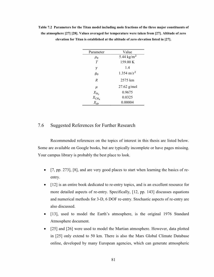
81

Table 7.2 Parameters for the Titan model including mole fractions of the three major constituents of

the atmosphere [27] [28]. Values averaged for temperature were taken from [27]. Altitude of zero

elevation for Titan is established at the altitude of zero elevation listed in [27].

Parameter Value <= 5.44 kg/m%

T 159.00 K

� 1.4

(= 1.354 m/½%

R 2575 km

; 27.62 g/mol

uv$ 0.9675

u,¾¿ 0.0325

ux\ 0.00004

7.6 Suggested References for Further Research

Recommended references on the topics of interest in this thesis are listed below.

Some are available on Google books, but are typically incomplete or have pages missing.

Your campus library is probably the best place to look.

• [7, pp. 273], [8], and are very good places to start when learning the basics of re-

entry.

• [12] is an entire book dedicated to re-entry topics, and is an excellent resource for

more detailed aspects of re-entry. Specifically, [12, pp. 143] discusses equations

and numerical methods for 3-D, 6 DOF re-entry. Stochastic aspects of re-entry are

also discussed.

• [13], used to model the Earth’s atmosphere, is the original 1976 Standard

Atmosphere document.

• [25] and [26] were used to model the Martian atmosphere. However, data plotted

in [25] only extend to 50 km. There is also the Mars Global Climate Database

online, developed by many European agencies, which can generate atmospheric

82

data for any location, time of year and day, and weather conditions on Mars. It is

available at http://www-mars.lmd.jussieu.fr/.

• [29] discusses systems for pinpoint landing on Mars.

• [27] and [28] were used to model Titan’s atmosphere.

• Re-entry and descent information on the Huygens probe, which landed

successfully on Titan in 2005, is included in [30]. The probe is also discussed

somewhat in [28]. NASA’s Jet Propulsion Laboratory also has reports that may be

available upon request on its website for the Cassini probe currently orbiting

Saturn, http://saturn.jpl.nasa.gov/.

• Books by Bryson and Hull are good general recourses on optimal control.

• [23, pp. 133] may be good to read before starting any studies involving stochastic

re-entry models.

• [31, pp. 737] describes equations for stagnation point heat flux under different

boundary layer and catalytic conditions in hypersonic flow. Also a good resource

for other re-entry heating topics.

The NASA History Division is a good place to start when searching for historical

documents, such as Apollo mission reports. They also list contact information, and it

would by wise to try and contact them if after an exhaustive search the data or

information sought after cannot be found. The website is http://history.nasa.gov/.

As far as getting re-entry data from actual missions to Mars, Titan or other places

of interest, data may be difficult to find online. The best bet is then to try and get in

contact with the agency or agencies in charge of the mission, such as the Jet Propulsion

Lab (JPL), the European Space Agency (ESA), or the supporting institutions such as the

California Institute of Technology or Georgia Tech, for example. Patience and persis-

tence are most likely needed in attempting to reach these agencies, so it would be wise to

plan accordingly and contact them as early as possible in the research process.

83

Epilogue

While writing this thesis, I have not only enjoyed paging through the old

historical documents of the 1960s and 70s on Apollo (and at the very least, better

understood the ending of the movie Apollo 13), but have enjoyed learning an incredible

amount about the current state of space politics in the United States.

As I write this, the fate of the manned space program is more uncertain than ever.

I was an intern at NASA Glenn Research Center in the summer of 2008, where I sat in on

a presentation to a large audience of employees about the progress of the constellation

program. I remember the presenter specifically saying “We are on track to have human

footprints on the moon by 2019.” I was excited by the prospect, and I thought NASA’s

plans were pretty set in stone. So when I flipped on NASA TV a year later to find the

Augustine Committee discussing the possible scrapping of the Constellation program and

various options that would replace it—I was honestly a little shocked. I’ve paid closer

attention to the political situation ever since, yet the more I learn about what influences

space policy, the more unanswered questions there seem to be.

Last February the new budget was rolled out, directing NASA to end

Constellation totally and switch to commercial companies for providing Astronauts

access to Low Earth Orbit (LEO), with few other details. On April 15th, President Obama

delivered a speech at Kennedy Space Center and outlined further details, including

bringing back the Orion capsule as a Crew Return Vehicle (CRV) for the space station,

technology development programs, and missions to deep space towards a Mars landing

decades from now. Even with these new details, it is hard to predict what other changes

will be made in this new plan, what actions congress will take in the next year, or

whether the deep space missions outlined for the next two decades will actually be

carried out.

I’m cautiously optimistic about the change in policy. With so much debate about

it, it is hard to decide who to believe (which I find interesting because I just spent the past

six years of my life getting two engineering degrees, yet my opinion on space policy still

84

depends on who I choose to believe). Why was constellation so far behind and over-

budget? Those supporting the program point out that it was underfunded, but considering

the design for Ares and Orion was based off of currently existing hardware from the

Shuttle and Apollo eras, I’m still skeptical as to the reason they’re not meeting their

deadlines. Fully funding Constellation would have also required splashing the Inter-

national Space Station in 2015, which would be a bad move considering the enormous

investment. I’m skeptical of some of the Augustine Committee findings as well, with

some prominent engineers claiming the cost estimates were far overblown, especially for

heavy lift development. There’s also reason to be skeptical of the claims made by the new

start-up space companies in the so-called “New Space” community. I applaud the bold

efforts of SpaceX and other companies, and I think there are good arguments to be made

for switching from cost-plus contracts to fixed-price contracts, but I still take some of

their statements with a grain of salt. I can also say the same thing of politicians on both

sides of the aisle, who often seem uninformed or only motivated by potential job losses in

their districts. Yet, who can blame them? From what the polls seem to indicate, the

majority of Americans like the space program, but a very small percentage actually pay

attention to it. In addition, considering the current financial state of the country, it is also

easy to see how half of those polled by Rasmussen on January 15th

of this year favored

cutting NASA’s budget.

Since Apollo, one of the main objectives in deciding which vehicle to develop has

been to bring down the cost of sending humans to LEO. Facilitating private industry to

provide access to LEO has much potential to this end, and has the potential to free up

more of NASA’s resources towards deep space exploration, which seems a more fitting

goal for an exploration agency that should be on the cutting edge.

Personally, I am not endorsing any particular plan yet as I am still forming my

opinion on it, but I do know this—we can’t change the rocket equation. The best we can

do is change the way we do business. A human space flight program that is “worthy of a

great nation” is one that makes access to space easier and more robust such that more of

the investment in space is returned to the people who pay for it—and hopefully, that

makes the benefits of space more visible to the public.

85

Whatever path is chosen for the space program, I sincerely hope we are able to

keep the human space flight program in existence, to make it more robust and

sustainable, and hopefully in my lifetime, to send humans to explore Mars and the rest of

the solar system. Considering the possibility of discovering life off the Earth, the known

resources that could be utilized in-situ to support a mission, and because of its similarity

to Earth in many respects, Mars is a destination that is worthy of being the current goal.

As the only known component of the universe that is able to truly understand itself and its

surroundings, we humans need to better understand the cosmos and our place within it.

The better a perspective we have on our home by exploring the solar system and the rest

of the universe, the better a chance we have of doing the right thing, making the right

choices, and making the best use of the incredible gift we have been given.

—Derrick Tetzman, May 11th

, 2010.

86

References

[1] Betts, John T., “Survey of Numerical Methods for Trajectory Optimization,” Journal

of Guidance, Control, and Dynamics, Vol. 21, No. 2, 1998, pp. 193-207

[2] Stoer, J. and Bulirsch, R., Introduction to Numerical Analysis, 3rd

ed., Springer-

Verlag, New York, 2002.

[3] Grimm, W. and Rot Àarmel, W., “Integrated Guidance and Control for Entry

Vehicles,” From Nano to Space, Applied Mathematics Inspired by Roland Bulirsch,

Springer-Verlag, Berlin Heidelberg, 2008, pp. 295-308.

[4] Betts, John T., Practical Methods for Optimal Control Using Nonlinear

Programming, Society for Industrial and Applied Mathematics, Philadelphia, 2001, pp.

133-138.

[5] Bonnans, J. and Launay, G., Large Scale Direct Optimal Control Applied to the Re-

entry Problem, Rapport de recherche, Program 5: Traitment du signal, automatique et

productique, No. 2402, Institut National De Recherche en Informatique et en

Automatique (INRIA) Rocquencourt, Le Chesnay, France, 1994.

[6] Hull, David G., Optimal Control Theory for Applications, Springer-Verlag, New

York, 2003.

[7] Griffin, Michael D. and French, James R., Space Vehicle Design, 2nd

ed., AIAA

Education Series, AIAA, Reston, VA, 2004.

[8] Anderson, John D., Jr, Introduction to Flight, 5th

ed., McGraw-Hill, New York, NY

2005.

[9] Allen, H. Julian and Eggers, A. J., Jr., “A Study of the Motion and Aerodynamic

Heating of Ballistic Missiles Entering the Earth’s Atmosphere at High Supersonic

Speeds”, NACA Report 1381, Ames Aeronautical Laboratory, Moffett Field, CA 1953.

[10] Fay, J. A. and Riddell, F. R., “Theory of Stagnation Point Heat Transfer in

Dissociated Air,” Journal of the Aeronautical Sciences, Vol. 25, No. 2, 1958, pp. 73-85,

121.

[11] Sutton, Kenneth and Graves, Randolph A., Jr., “A General Stagnation-Point

Convective Heating Equation for Arbitrary Gas Mixtures,” NASA TR R-376, Langley

Research Center, Hampton, VA, 1971.

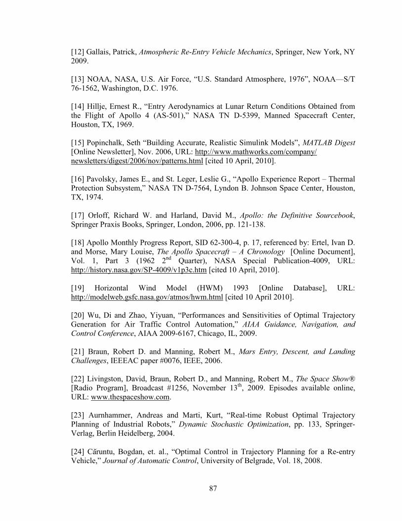
87

[12] Gallais, Patrick, Atmospheric Re-Entry Vehicle Mechanics, Springer, New York, NY

2009.

[13] NOAA, NASA, U.S. Air Force, “U.S. Standard Atmosphere, 1976”, NOAA—S/T

76-1562, Washington, D.C. 1976.

[14] Hillje, Ernest R., “Entry Aerodynamics at Lunar Return Conditions Obtained from

the Flight of Apollo 4 (AS-501),” NASA TN D-5399, Manned Spacecraft Center,

Houston, TX, 1969.

[15] Popinchalk, Seth “Building Accurate, Realistic Simulink Models”, MATLAB Digest

[Online Newsletter], Nov. 2006, URL: http://www.mathworks.com/company/

newsletters/digest/2006/nov/patterns.html [cited 10 April, 2010].

[16] Pavolsky, James E., and St. Leger, Leslie G., “Apollo Experience Report – Thermal

Protection Subsystem,” NASA TN D-7564, Lyndon B. Johnson Space Center, Houston,

TX, 1974.

[17] Orloff, Richard W. and Harland, David M., Apollo: the Definitive Sourcebook,

Springer Praxis Books, Springer, London, 2006, pp. 121-138.

[18] Apollo Monthly Progress Report, SID 62-300-4, p. 17, referenced by: Ertel, Ivan D.

and Morse, Mary Louise, The Apollo Spacecraft – A Chronology [Online Document],

Vol. 1, Part 3 (1962 2nd

Quarter), NASA Special Publication-4009, URL:

http://history.nasa.gov/SP-4009/v1p3c.htm [cited 10 April, 2010].

[19] Horizontal Wind Model (HWM) 1993 [Online Database], URL:

http://modelweb.gsfc.nasa.gov/atmos/hwm.html [cited 10 April 2010].

[20] Wu, Di and Zhao, Yiyuan, “Performances and Sensitivities of Optimal Trajectory

Generation for Air Traffic Control Automation,” AIAA Guidance, Navigation, and

Control Conference, AIAA 2009-6167, Chicago, IL, 2009.

[21] Braun, Robert D. and Manning, Robert M., Mars Entry, Descent, and Landing

Challenges, IEEEAC paper #0076, IEEE, 2006.

[22] Livingston, David, Braun, Robert D., and Manning, Robert M., The Space Show®

[Radio Program], Broadcast #1256, November 13th

, 2009. Episodes available online,

URL: www.thespaceshow.com.

[23] Aurnhammer, Andreas and Marti, Kurt, “Real-time Robust Optimal Trajectory

Planning of Industrial Robots,” Dynamic Stochastic Optimization, pp. 133, Springer-

Verlag, Berlin Heidelberg, 2004.

[24] Caruntu, Bogdan, et. al., “Optimal Control in Trajectory Planning for a Re-entry

Vehicle,” Journal of Automatic Control, University of Belgrade, Vol. 18, 2008.

88

[25] Justh, H. L. and Justus, C. G., “Mars Global Reference Atmospheric Model (Mars-

GRAM 2005) Applications for Mars Science Laboratory Mission Site Selection

Processes”, Seventh International Conference on Mars, Caltech, 2007.

[26] Barlow, Nadine G., Mars, an Introduction to its Interior, Surface and Atmosphere,

Cambridge University Press, New York, NY, 2008.

[27] R. V. Yelle et. al., “Engineering Models for Titan’s Atmosphere”, 1997ESASP1177

243Y, 1997.

[28] Coustenis, Athena and Taylor, Fredric W., Titan: Exploring an Earthlike World,

World Scientific, Singapore, 2008.

[29] Wolf, Aron A. et. al., “Systems for Pinpoint Landing at Mars,” AAS 04-272, 2004.

[30] Kazeminejad, Bobby et. al., “Huygens’ entry and descent through Titan’s

atmosphere—Methodology and results of the trajectory reconstruction,” Planetary and

Space Science, vol. 55, pp. 1845-1876, 2007.

[31] Anderson, John D., Jr., Hypersonic and High Temperature Gas Dynamics Second

Edition, AIAA Education Series, AIAA, Reston, VA, 2006.

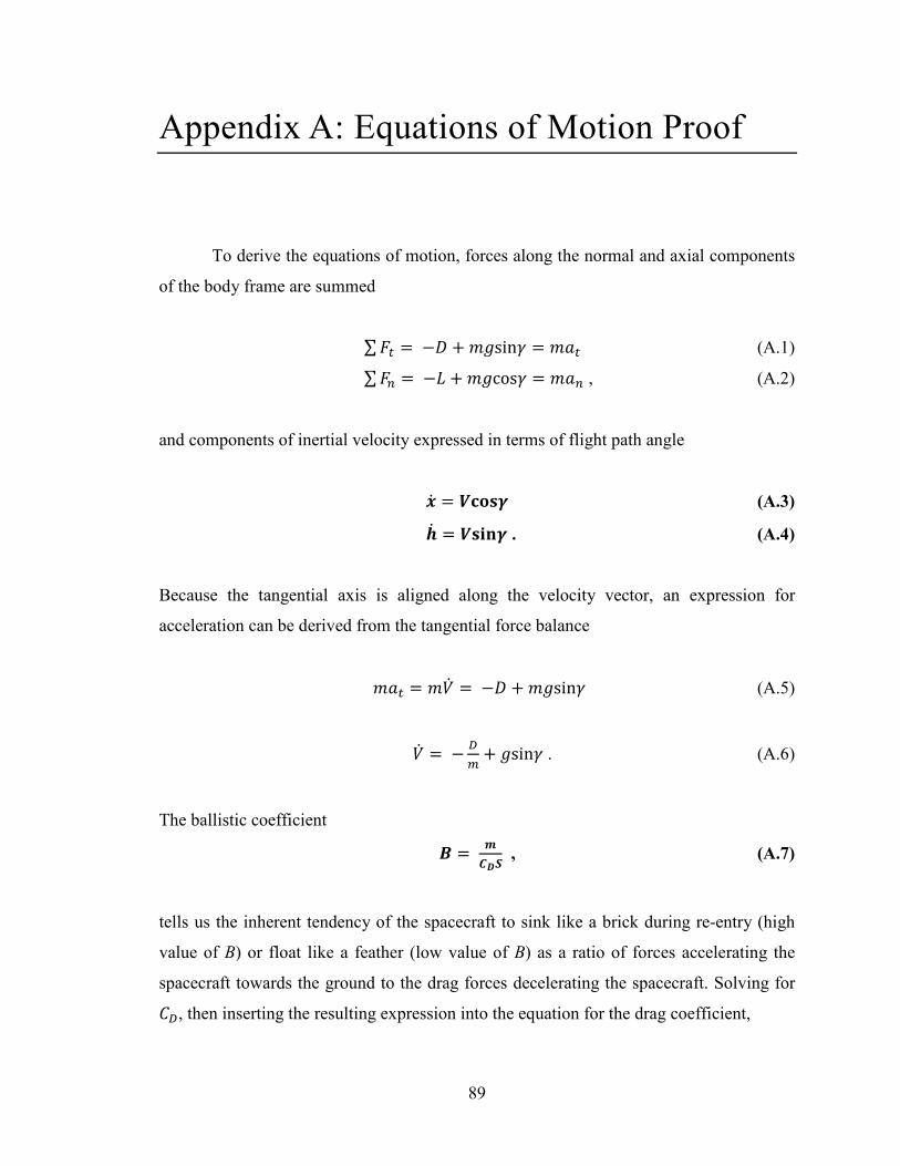
89

Appendix A: Equations of Motion Proof

To derive the equations of motion, forces along the normal and axial components

of the body frame are summed

∑ Ã] � !} ' ¼(sin� � ¼K] (A.1)

∑ Ãc � !U ' ¼(cos� � ¼Kc , (A.2)

and components of inertial velocity expressed in terms of flight path angle

�� � ÄÅÆÇ� (A.3)

�� � ÄÇÈÉ� . (A.4)

Because the tangential axis is aligned along the velocity vector, an expression for

acceleration can be derived from the tangential force balance

¼K] � ¼�� � !} ' ¼(sin� (A.5)

�� � ! 0+ ' (sin� . (A.6)

The ballistic coefficient

Ê � �ËÌ� , (A.7)

tells us the inherent tendency of the spacecraft to sink like a brick during re-entry (high

value of B) or float like a feather (low value of B) as a ratio of forces accelerating the

spacecraft towards the ground to the drag forces decelerating the spacecraft. Solving for

/0, then inserting the resulting expression into the equation for the drag coefficient,

90

/0 � 0�$"#$. , (A.8)

then substitute that expression into Eq. (A.5), we arrive at a very useful expression for

acceleration

Ä� � ! ÍÄ��Ê ' ÎÇÈÉÏ . (A.9)

To derive the flight path angular velocity, we start with the equation for the normal and

tangential components of the spacecraft’s acceleration along the flight path:

K � Ð#��Ð] � �� >] ' �>]� . (A.10)

The rotation of the body frame, and the rotation of the local frame about the fixed frame

must be taken into account, thus we define a new angular velocity

Ò � !1Ó� ' ��4 . (A.11)

The rate of change of the tangential unit vector can be expressed in terms of Ò as shown

in Figure A.1 for the spacecraft at an instantaneous moment in time.

91

Figure A.1 Geometry of body frame rotation. The flight path angle is corrected for � in the simulation with each calculation of �� .

Once �� is calculated, then integrated with respect to time during the simulation to find the

instantaneous value of �, this difference is taken into account. Knowing that the change

in direction of >] as it rotates is the normal unit vector

>c � Ð^ZÐ�ÔI9� , (A.12)

we can break down >] into components of >c. Let s equal the distance along the flight

path. Velocity � is then defined to include the change in distance s along the flight path

over time, and the change in the total angle (Ó ' �) over distance s

Ð^ZÐ] � Ð^Z

Ð�ÔI9�Ð�ÔI9�

ÐÕÐÕÐ] . (A.13)

Making the substitution

º�Ó ' �� � !Òº� , (A.14)

92

then cancelling out the ds and dt terms, we arrive at an expression for the rate of change

of the tangential unit vector in terms of Ò and the normal unit vector

Ð^ZÐ] � !Ò>c , (A.15)

which can be substituted for >]� in Eq. (A.10)

K � Ð#��Ð] � �� >] ! �Ò>c . (A.16)

Another way to express the acceleration

K � K]>] ' Kc>c , (A.17)

is equivalent to Eq. (A.16). Substituting Eq. (A.11) for Ò in Eq. (A.16), the normal

component of acceleration Kc becomes

Kc � ?�1� ' ��4C >c . (A.18)

The angular velocity associated with the rotation of the body frame about the fixed axis is

Ó� � #6789: , (A.19)

thus the expression for Kc now becomes

Kc � ?#$6789: ' ���C >c . (A.20)

When substituted into the equation for the forces along the normal axis, along with

expressing lift in terms of the lift coefficient,

93

U � T% /2<�%� , (A.21)

eq. (A.2) becomes

¼ ?#$6789: ' ���C � ! T

% /2<�%� ' ¼(cos� , (A.22)

solving for ��

�� � ! "#,Ö.%+ ' 5 6789

# ! # 678 9: , (A.23)

and substituting in ballistic and drag coefficients into the first term

T&,- � .

+ , (A.24)

the first term becomes ! "#?,Ö ,-3 C%& . /2 /0⁄ is the same as the lift to drag ratio, thus the

final expression for the flight path angular velocity is

�� � ! ÍÄ1� Ì3 4�Ê ' Î ÅÆÇ�

Ä ! Ä ÅÆÇ �Ø . (A.25)

94

Appendix B: Heat Flux Derivation

To derive the equation used for stagnation point heat flux, we start with the basic

convective heat transfer equation

R� � � ΔN , (B.1)

where R� is the surface heat flux in W/m%, ∆N is the change in temperature in K, and h is

the convective heat transfer coefficient in kg/s�K, whose value can be found through the

expression

� � ?� Mc3 C ¦� ΔN , (B.2)

where k is the thermal conductivity of the gas in kg-m/s�K, Mc is the nose radius for the

vehicle in meters (defined as the radius of curvature of the nose) and Nu is the non-

dimensional Nusselt number. The Nusselt number as derived by Allen and Eggers after

applying assumption 10 is:

¦� ~ M>T %3 � Û"#:bG , (B.3)

where Re is the Reynolds number. From conservation of energy of a fluid

> � ¨�NS ' #$% � ¨�N , (B.4)

where ¨� is the specific heat in ½@%Ü@T, and NS and N are freestream and boundary

layer edge (at the stagnation point) temperatures, respectively in Kelvin. It is reasonable

to assume:

95

14. N _ NS, and N _ N , the wall temperature.

After simplifying both Eq. (B.4)

N � #$%,Ý , (B.5)

and Eq. (B.1), then substituting Eq. (B.4) and Eq. (B.5) into the simplified Eq. (B.1)

R� � ?� Mc3 C ¦� N

R� � ?� Mc3 C Û"#:bG #$

%,Ý

R� � ?� Mc3 C Û"#:bG #$

%,Ý . (B.6)

From basic convective heat transfer, we take the expression for the Prandtl number

Þ� � GßÝ� , (B.7)

solve for the thermal conductivity k, apply assumption 13 that the Prandtl number is one,

then substitute this expression into Eq. (B.6) and simplify, the equation for heat flux now

becomes

R� � Û"G:b #à/$

%,Ý . (B.8)

From kinetic theory for fluids

; ¯ /TNT/% , (B.9)

96

where /T is a constant. Substituting Eq. (B.5) for NÕ, then substituting the resulting exp-

ression for ; in Eq. (B.8), we end up with

R� � oT% Û ,�

%ßÝt á#aL"L:b â . (B.10)

After combining the first term as a single constant C, we arrive at the equation for re-

entry heat flux

�� � ËÄãLÍLØ­ . (B.11)

97

Appendix C: Exponential Density Model

The derivation of this model begins with the equation of hydrostatic equilibrium

for the atmosphere

Ð�ÐJ � !<(. (C.1)

where p is pressure. The equation for density of a gas is

< � c Gä , (C.2)

where n is the number of moles, ; is the molar mass, and · is volume. Solving for n and

substituting the expression into the ideal gas law

å· � �MN, (C.3)

where R = 8.314 J/mol-K is the ideal gas constant and T is temperature, yields an

expression for density in terms of pressure, molecular mass, the ideal gas constant and

temperature

< � �G:F . (C.4)

Substituting Eq. (C.4) into Eq. (C.1)

�� � ! G5

:F ºæ, (C.5)

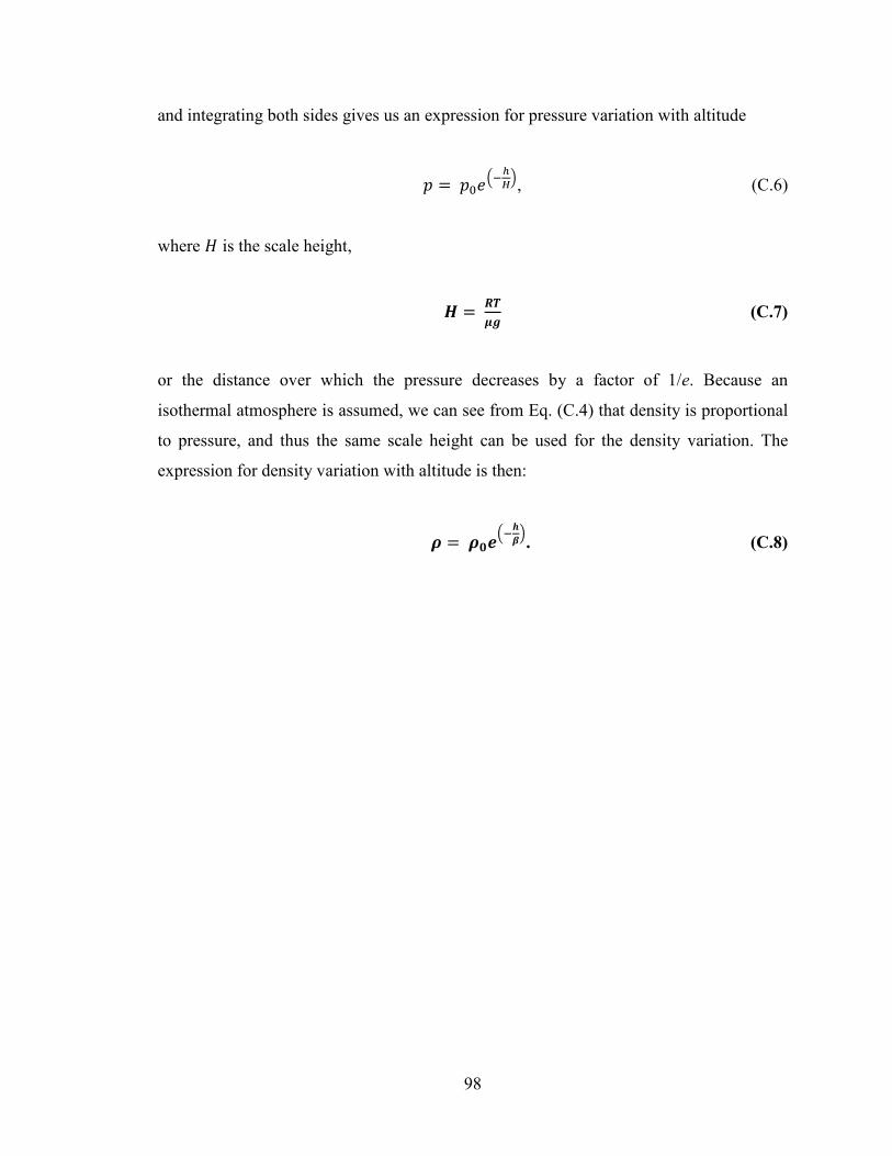
98

and integrating both sides gives us an expression for pressure variation with altitude

å � å=>?@ABC

, (C.6)

where E is the scale height,

ç � ØèéÎ (C.7)

or the distance over which the pressure decreases by a factor of 1/e. Because an

isothermal atmosphere is assumed, we can see from Eq. (C.4) that density is proportional

to pressure, and thus the same scale height can be used for the density variation. The

expression for density variation with altitude is then:

Í � Í �?@�êC. (C.8)

99

Appendix D: Opt. Study Results Tables

Table D.1 Results from Chapter 6 undershoot case. Runtime difference between results listed in this

table from Table 6.3 are due to other programs being run on the same computer while the test was

conducted. This was the only instance of this. Conditions are otherwise the same for each test in a

series.

# Intervals Run Time (s) # Iterations Optimum Input

1 257.2 218 0.22527

2 421.8 238 0.22649

0.20261

3 568.6 236

0.22652

0.20247

0.20297

4 705.7 233

0.22659

0.2046

0.20493

0.20486

5 804.6 222

0.2268

0.20922

0.23516

0.2085

0.21229

6 791.0 190

0.22718

0.21682

0.26189

0.23578

0.21083

0.22336

100

Table D.2 Results from Chapter 6 for the overshoot case.

# Intervals Run Time (s) # Iterations Optimum Input

1 212.8 171 0.22532

2 366.8 193 0.22448

0.24007

3 499.9 196

0.22443

0.23974

0.24048

4 739.6 233

0.22418

0.24414

0.23991

0.24493

5 817.8 213

0.22393

0.23258

0.24842

0.24444

0.24076

101

Table D.3 Results from Chapter 6 for the undershoot with wind case.

# Intervals Run Time (s) # Iterations Optimum Input

1 375.9 207 0.2205

2 641.3 231 0.22153

0.2022

3 848 228

0.22155

0.20202

0.2024

4 1003.6 225

0.22161

0.20477

0.20366

0.20363

5 1148.9 215

0.2219

0.20651

0.21778

0.20613

0.20804

6 1228.7 198

0.22228

0.21213

0.25006

0.22814

0.20921

0.22074

7 2695.7 358

0.2209

0.22239

0.30675

0.47463

0.18366

0.19914

0.15897

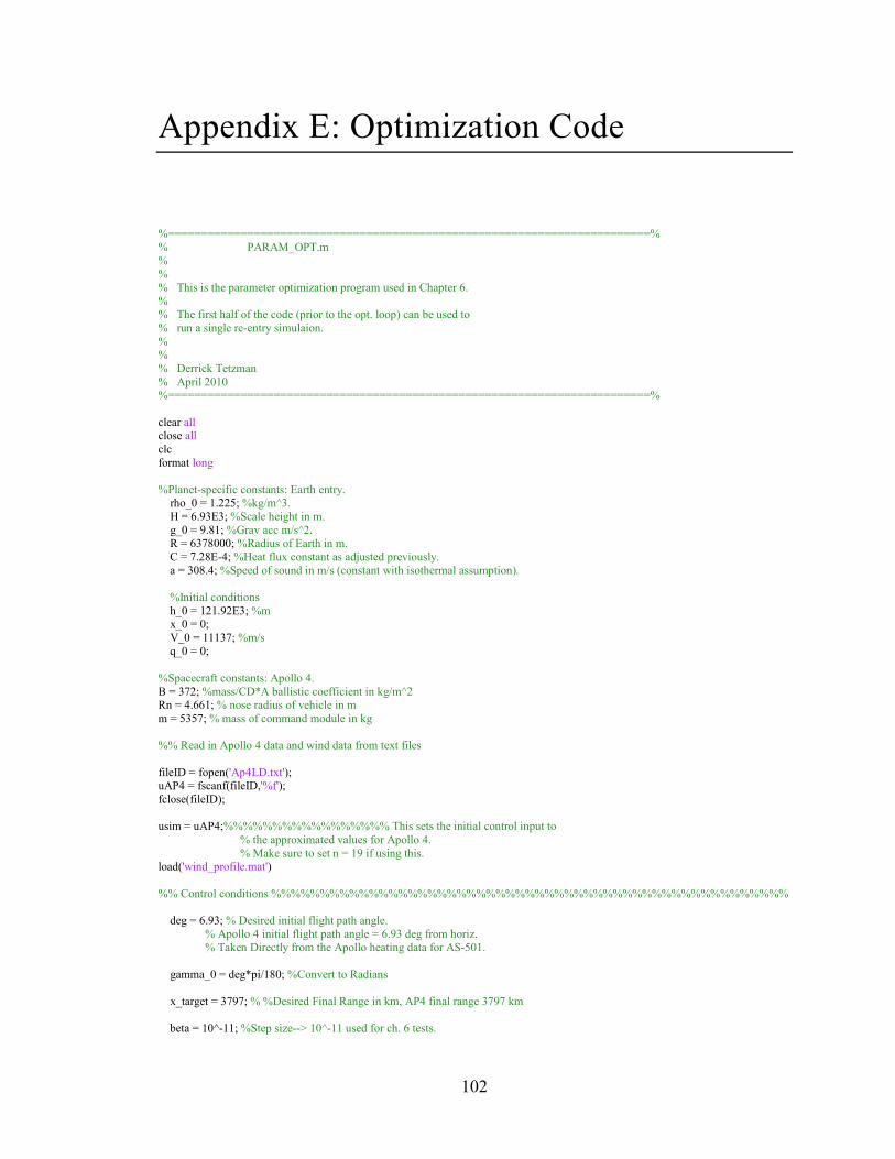
102

Appendix E: Optimization Code

%=========================================================================%

% PARAM_OPT.m

% %

% This is the parameter optimization program used in Chapter 6.

% % The first half of the code (prior to the opt. loop) can be used to

% run a single re-entry simulaion.

% %

% Derrick Tetzman

% April 2010 %=========================================================================%

clear all close all

clc

format long

%Planet-specific constants: Earth entry. rho_0 = 1.225; %kg/m^3.

H = 6.93E3; %Scale height in m.

g_0 = 9.81; %Grav acc m/s^2. R = 6378000; %Radius of Earth in m.

C = 7.28E-4; %Heat flux constant as adjusted previously.

a = 308.4; %Speed of sound in m/s (constant with isothermal assumption).

%Initial conditions

h_0 = 121.92E3; %m x_0 = 0;

V_0 = 11137; %m/s

q_0 = 0;

%Spacecraft constants: Apollo 4.

B = 372; %mass/CD*A ballistic coefficient in kg/m^2 Rn = 4.661; % nose radius of vehicle in m

m = 5357; % mass of command module in kg

%% Read in Apollo 4 data and wind data from text files

fileID = fopen('Ap4LD.txt'); uAP4 = fscanf(fileID,'%f');

fclose(fileID);

usim = uAP4;%%%%%%%%%%%%%%%%% This sets the initial control input to

% the approximated values for Apollo 4.

% Make sure to set n = 19 if using this. load('wind_profile.mat')

%% Control conditions %%%%%%%%%%%%%%%%%%%%%%%%%%%%%%%%%%%%%%%%%%%%%%%%%%%%%

deg = 6.93; % Desired initial flight path angle.

% Apollo 4 initial flight path angle = 6.93 deg from horiz. % Taken Directly from the Apollo heating data for AS-501.

gamma_0 = deg*pi/180; %Convert to Radians

x_target = 3797; % %Desired Final Range in km, AP4 final range 3797 km

beta = 10^-11; %Step size--> 10^-11 used for ch. 6 tests.

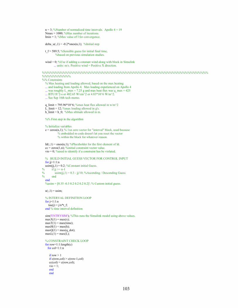
103

n = 3; %Number of normalized time intervals. Apollo 4 = 19

Nmax = 1000; %Max number of iterations. Imin = 1; %Max value of I for convergence.

delta_u(:,1) = -0.2*ones(n,1); %Initial step

t_f = 589.5; %Sensible guess for initial final time,

%based on previous simulation studies.

wind = 0; %Use if adding a constant wind along with block in Simulink

... units: m/s. Positive wind = Positive X direction.

%%%%%%%%%%%%%%%%%%%%%%%%%%%%%%%%%%%%%%%%%%%%%%%%%%%%%%%%%%%%%%%%

%%%%%%%%%%% %% Constraints

% Max heating and loading allowed, based on the max heating

... and loading from Apollo 4. Max loading experienced on Apollo 4 ... was roughly L_max = 7.25 g and max heat flux was q_max = 425

... BTU/ft^2-s or 482.65 W/cm^2 or 4.83*10^6 W/m^2.

... See Sep 16th tech memo.

q_limit = 795.96*10^6; %max heat flux allowed in w/m^2

L_limit = 12; %max loading allowed in g's. h_limit = h_0; %Max altitude allowed in m.

%% First step in the algorithm

% Initialize variables e = zeros(n,1); % 1xn zero vector for "interval" block, used because

% embedded m-code doesn't let you reset the vector

% within the block for whatever reason.

Id(:,1) = ones(n,1); %Placeholder for the first element of Id.

cc = zeros(1,n); %initial constraint vector value. vio = 0; %used to identify if a constraint has be violated.

% BUILD INITIAL GUESS VECTOR FOR CONTROL INPUT for jj=1:1:n

usim(jj,1) = 0.2; %Constant initial Guess.

% if jj >= n-1 % usim(jj,1) = 0.3 - jj/10; %Ascending / Descending Guess

% end

end %usim = [0.35 -0.3 0.2 0.2 0.2 0.2]'; % Custom initial guess.

u(:,1) = usim;

% INTERVAL DEFINITION LOOP

for j=1:1:n tau(j) = j/n*t_f;

end % time interval definition

sim('ENTRYSIM'); %This runs the Simulink model using above values.

maxX(1) = max(x);

maxT(1) = max(time); maxH(1) = max(h);

maxQ(1) = max(q_dot);

maxL(1) = max(L);

% CONSTRAINT CHECK LOOP

for row=1:1:length(c) for col=1:1:n

if row > 1 if c(row,col) > c(row-1,col)

cc(col) = c(row,col);

vio = 1; end

end

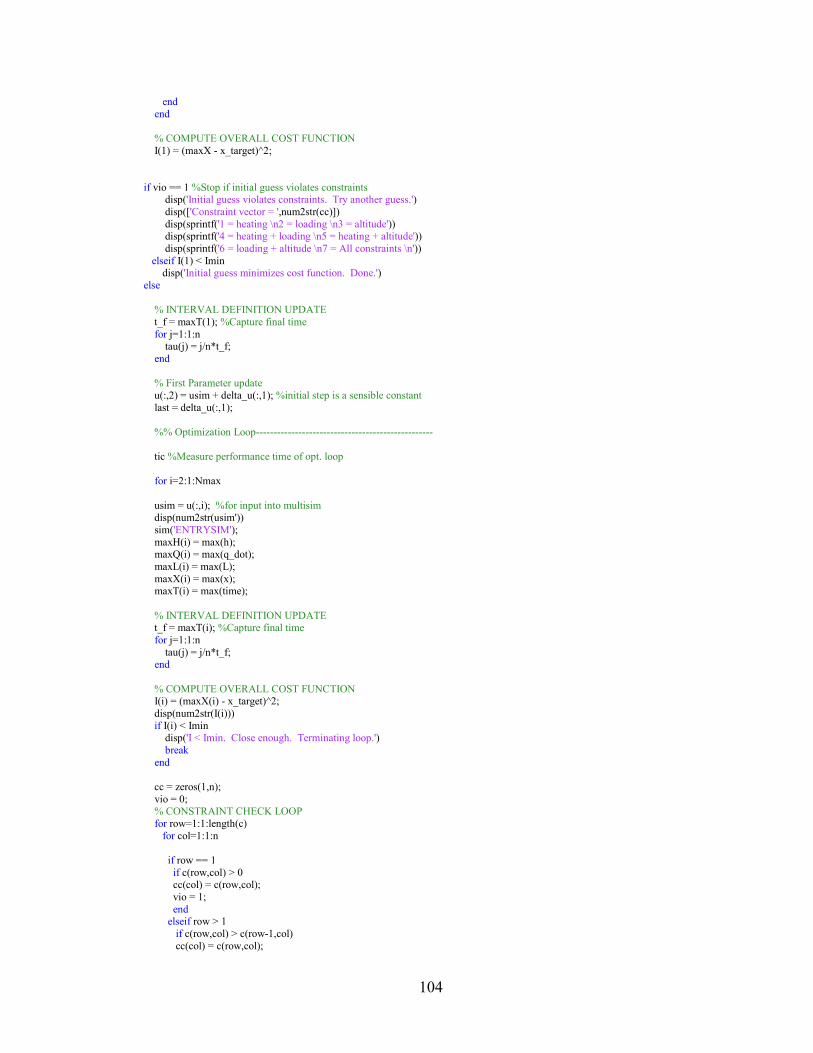
104

end

end

% COMPUTE OVERALL COST FUNCTION

I(1) = (maxX - x_target)^2;

if vio == 1 %Stop if initial guess violates constraints disp('Initial guess violates constraints. Try another guess.')

disp(['Constraint vector = ',num2str(cc)])

disp(sprintf('1 = heating \n2 = loading \n3 = altitude')) disp(sprintf('4 = heating + loading \n5 = heating + altitude'))

disp(sprintf('6 = loading + altitude \n7 = All constraints \n'))

elseif I(1) < Imin disp('Initial guess minimizes cost function. Done.')

else

% INTERVAL DEFINITION UPDATE

t_f = maxT(1); %Capture final time

for j=1:1:n tau(j) = j/n*t_f;

end

% First Parameter update

u(:,2) = usim + delta_u(:,1); %initial step is a sensible constant

last = delta_u(:,1);

%% Optimization Loop--------------------------------------------------

tic %Measure performance time of opt. loop

for i=2:1:Nmax

usim = u(:,i); %for input into multisim disp(num2str(usim'))

sim('ENTRYSIM');

maxH(i) = max(h); maxQ(i) = max(q_dot);

maxL(i) = max(L);

maxX(i) = max(x); maxT(i) = max(time);

% INTERVAL DEFINITION UPDATE t_f = maxT(i); %Capture final time

for j=1:1:n

tau(j) = j/n*t_f; end

% COMPUTE OVERALL COST FUNCTION I(i) = (maxX(i) - x_target)^2;

disp(num2str(I(i)))

if I(i) < Imin disp('I < Imin. Close enough. Terminating loop.')

break

end

cc = zeros(1,n);

vio = 0; % CONSTRAINT CHECK LOOP

for row=1:1:length(c)

for col=1:1:n

if row == 1

if c(row,col) > 0 cc(col) = c(row,col);

vio = 1;

end elseif row > 1

if c(row,col) > c(row-1,col)

cc(col) = c(row,col);

105

vio = 1;

end end

end end

if vio == 1 disp(num2str(cc))

end

disp(' ')

if i == Nmax %value reached after Nmax iterations disp('Max number of iterations reached. i = Nmax.')

break % Further update unnecessary.

end

% DERIVATIVE / PARAMETER UPDATE LOOP ------

t_f = maxT(i-1); % Use previous final time

for j=1:1:n tau(j) = j/n*t_f;

end

for k=1:1:n

if (cc(k) ~= 0) %Constraint Control

% ADD CONSTRAINT LOGIC HERE %

% EXAMPLE BRUTE FORCE METHOD I USED:

if (cc(k)==1) || (cc(k)==2) || (cc(k)==4) u(k,i+1) = u(k,i) + 0.1;

if k ~= 1

u(k-1,i+1) = u(k-1,i+1) + 0.0001 ; end

elseif cc(k)==3 u(k,i+1) = u(k,i) - 0.1 ;

if k ~= 1

u(k-1,i+1) = u(k-1,i+1) - 0.001 ; end

else u(k,i+1) = u(k,i-1);

end

Id(k,i) = 10^-6; %Placeholder for the derivative array

elseif (u(k,i) == u(k,i-1)) u(k,i+1) = u(k,i) - 10^-3;

disp('NO UPDATE!')

disp(['interval = ',num2str(k)]) beep

%Alerts the user if algorithm gets stuck.

%This typically happens when the spacecraft skips out. else

usim = u(:,i-1);

usim(k) = u(k,i); sim('ENTRYSIM')

maxsX = max(x);

Id(k,i) = ((maxsX - x_target)^2-I(i-1)) / (usim(k)-u(k,i-1));

if Id(k,i) == 0

Id(k,i) = 10^-4; end

% PARAMETER UPDATE

106

delta_u(k,i) = -beta * Id(k,i);

u(k,i+1) = u(k,i) + delta_u(k,i); last = delta_u(:,i);

end

end

t_f = maxT(i); %Switch back for the next loop iteration.

for j=1:1:n tau(j) = j/n*t_f;

end

% Note: it might seem strange to have these additional loops ...for tau just for the derivative loop, but it saves memory

...by eliminating the need to store yet ANOTHER large array.

end

%% Display Results MODIFIED FOR ONLY ONE RUN THROUGH!

disp('************* RESULTS **************') disp(' ')

disp(['For n = ',num2str(n)])

disp(' ')

if vio == 1

disp('Constraints violated.') disp(['Constraint vector = ', num2str(cc)])

disp(sprintf('1 = heating \n2 = loading \n3 = altitude')) disp(sprintf('4 = heating + loading \n5 = heating + altitude'))

disp(sprintf('6 = loading + altitude \n7 = All constraints \n'))

else disp('No constraint violations.')

end

toc

disp(' ') disp(['# Iterations: ',num2str(i)])

disp(' ')

disp('The optimum values of L/D are:') disp(num2str(u(:,i)))

disp(' ')

disp('The final cost function value is:') disp(['I = ',num2str(I(i))])

disp(' ')

disp('With a corresponding final range of:') disp(['x_final = ',num2str(maxX(i))])

%% Read in Approximate AP4 Trajectory XY reconstruction

fileIDX = fopen('AP4apxrecX.txt');

fileIDY = fopen('AP4apxrecY.txt'); Xrec = fscanf(fileIDX,'%f');

Yrec = fscanf(fileIDY,'%f');

fclose(fileIDX); fclose(fileIDY);

%% Plot

% Plot Final Trajectory

figure5 = figure('Color',[1 1 1]); hold on

plot(x,h,'b','DisplayName','Simulated Trajectory');

plot(Xrec,Yrec,'k','DisplayName','Approx. Reconstruction'); grid on; xlabel('Range (km)'); ylabel('Altitude (km)');

title('Final Trajectory');

hold off

end % For the initial constraint violation check.

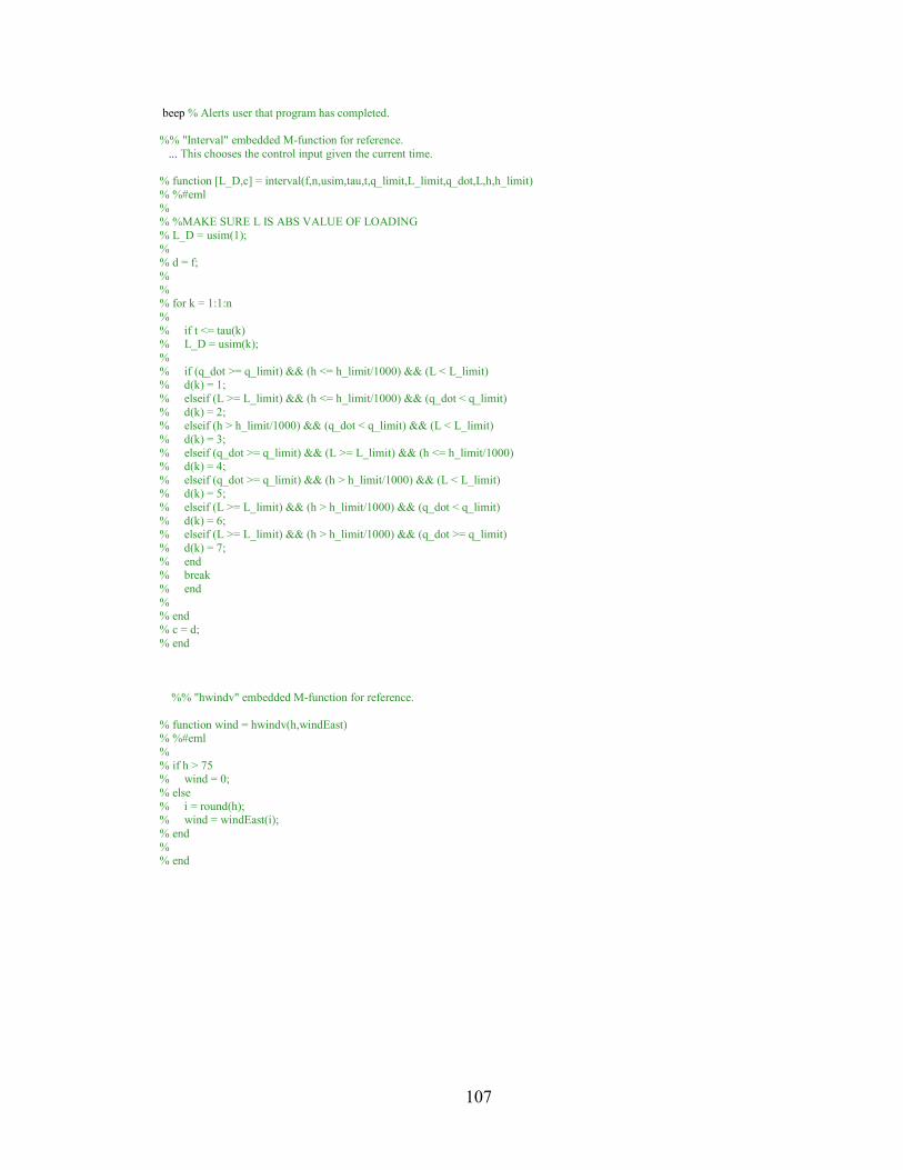
107

beep % Alerts user that program has completed.

%% "Interval" embedded M-function for reference.

... This chooses the control input given the current time.

% function [L_D,c] = interval(f,n,usim,tau,t,q_limit,L_limit,q_dot,L,h,h_limit)

% %#eml

% % %MAKE SURE L IS ABS VALUE OF LOADING

% L_D = usim(1);

% % d = f;

%

% % for k = 1:1:n

%

% if t <= tau(k) % L_D = usim(k);

%

% if (q_dot >= q_limit) && (h <= h_limit/1000) && (L < L_limit) % d(k) = 1;

% elseif (L >= L_limit) && (h <= h_limit/1000) && (q_dot < q_limit)

% d(k) = 2; % elseif (h > h_limit/1000) && (q_dot < q_limit) && (L < L_limit)

% d(k) = 3;

% elseif (q_dot >= q_limit) && (L >= L_limit) && (h <= h_limit/1000) % d(k) = 4;

% elseif (q_dot >= q_limit) && (h > h_limit/1000) && (L < L_limit) % d(k) = 5;

% elseif (L >= L_limit) && (h > h_limit/1000) && (q_dot < q_limit)

% d(k) = 6; % elseif (L >= L_limit) && (h > h_limit/1000) && (q_dot >= q_limit)

% d(k) = 7;

% end % break

% end

% % end

% c = d;

% end

%% "hwindv" embedded M-function for reference.

% function wind = hwindv(h,windEast) % %#eml

%

% if h > 75 % wind = 0;

% else

% i = round(h); % wind = windEast(i);

% end

% % end

108

Appendix F: Simulink Model

Figure F.1 Gravity and density calculations.

109

Figure F.2 Interval m-function, absolute acceleration and flight path angular velocity equations.

110

Figure F.3 Calculations for vertical and horizontal components of velocity, freestream velocity, and

stag. pt. heat flux.

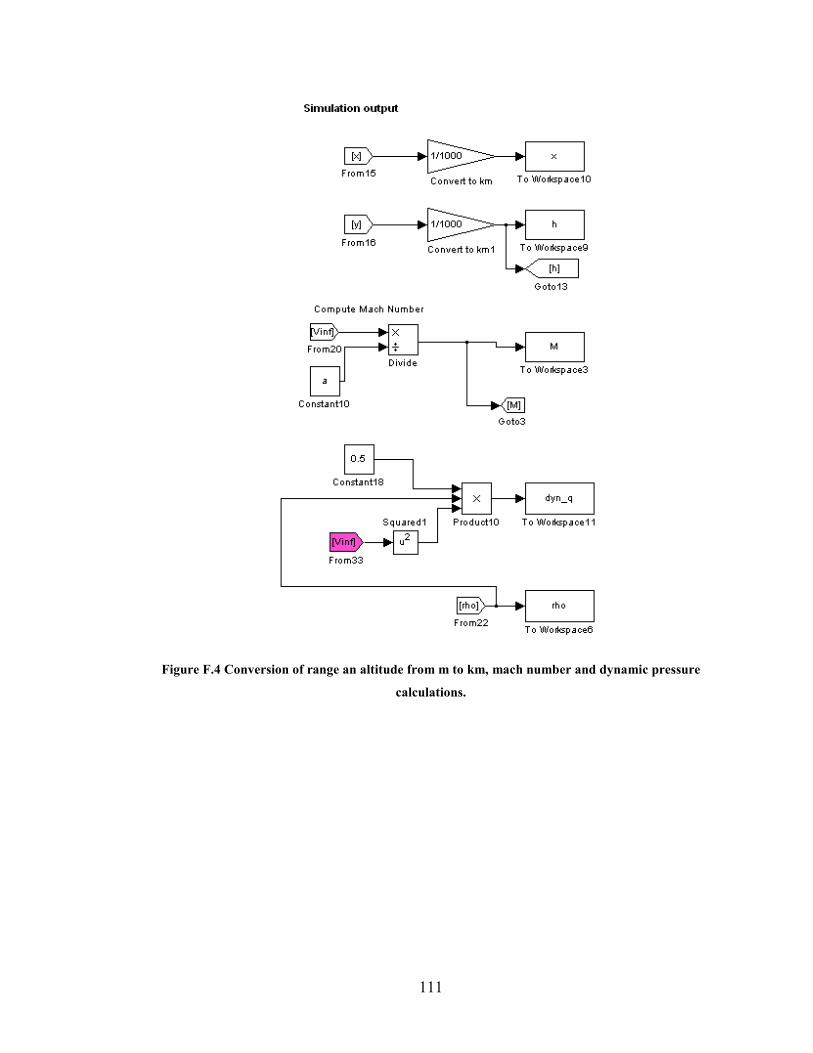
111

Figure F.4 Conversion of range an altitude from m to km, mach number and dynamic pressure

calculations.

112

Figure F.5 Loading calculation, heat flux and flight path angle fed to workspace, and stop simulation

conditions.

113

Figure F.6 Correction to velocity and flight path angle for wind, branch extending from “hwindv” m-

function fed into freestream velocity equation.