Text Classi cation from Labeled and Unlabeled …knigam/papers/emcat-mlj99.pdfMachine Learning, , 1{34 Kluwer Academic Publishers, Boston. Manufactured in The Netherlands.c Text Classi

Machine Learning, , 1–34 ()c© Kluwer Academic Publishers, Boston. Manufactured in The Netherlands.

Text Classification from Labeled and UnlabeledDocuments using EM

KAMAL NIGAM† [email protected]

ANDREW KACHITES MCCALLUM‡† [email protected]

SEBASTIAN THRUN† [email protected]

TOM MITCHELL† [email protected]

†School of Computer Science, Carnegie Mellon University, Pittsburgh, PA 15213‡Just Research, 4616 Henry Street, Pittsburgh, PA 15213

Received March 15, 1998; Revised February 20, 1999

Editor: William W. Cohen

Abstract. This paper shows that the accuracy of learned text classifiers can be improved byaugmenting a small number of labeled training documents with a large pool of unlabeled docu-ments. This is important because in many text classification problems obtaining training labelsis expensive, while large quantities of unlabeled documents are readily available.

We introduce an algorithm for learning from labeled and unlabeled documents based on thecombination of Expectation-Maximization (EM) and a naive Bayes classifier. The algorithm firsttrains a classifier using the available labeled documents, and probabilistically labels the unlabeleddocuments. It then trains a new classifier using the labels for all the documents, and iteratesto convergence. This basic EM procedure works well when the data conform to the generativeassumptions of the model. However these assumptions are often violated in practice, and poorperformance can result. We present two extensions to the algorithm that improve classificationaccuracy under these conditions: (1) a weighting factor to modulate the contribution of theunlabeled data, and (2) the use of multiple mixture components per class. Experimental results,obtained using text from three different real-world tasks, show that the use of unlabeled datareduces classification error by up to 30%.

Keywords: text classification, Expectation-Maximization, integrating supervised and unsuper-vised learning, combining labeled and unlabeled data, Bayesian learning

1. Introduction

Consider the problem of automatically classifying text documents. This problemis of great practical importance given the massive volume of online text avail-able through the World Wide Web, Internet news feeds, electronic mail, corporatedatabases, medical patient records and digital libraries. Existing statistical textlearning algorithms can be trained to approximately classify documents, given asufficient set of labeled training examples. These text classification algorithms havebeen used to automatically catalog news articles (Lewis & Gale, 1994; Joachims,1998) and web pages (Craven, DiPasquo, Freitag, McCallum, Mitchell, Nigam, &Slattery, 1998; Shavlik & Eliassi-Rad, 1998), automatically learn the reading in-terests of users (Pazzani, Muramatsu, & Billsus, 1996; Lang, 1995), and automati-

2 NIGAM, MCCALLUM, THRUN AND MITCHELL

cally sort electronic mail (Lewis & Knowles, 1997; Sahami, Dumais, Heckerman, &Horvitz, 1998).

One key difficulty with these current algorithms, and the issue addressed by thispaper, is that they require a large, often prohibitive, number of labeled trainingexamples to learn accurately. Labeling must often be done by a person; this is apainfully time-consuming process.

Take, for example, the task of learning which UseNet newsgroup articles are ofinterest to a particular person reading UseNet news. Systems that filter or pre-sortarticles and present only the ones the user finds interesting are highly desirable,and are of great commercial interest today. Work by Lang (1995) found that after aperson read and labeled about 1000 articles, a learned classifier achieved a precisionof about 50% when making predictions for only the top 10% of documents aboutwhich it was most confident. Most users of a practical system, however, wouldnot have the patience to label a thousand articles—especially to obtain only thislevel of precision. One would obviously prefer algorithms that can provide accurateclassifications after hand-labeling only a few dozen articles, rather than thousands.

The need for large quantities of data to obtain high accuracy, and the difficultyof obtaining labeled data, raises an important question: what other sources ofinformation can reduce the need for labeled data?

This paper addresses the problem of learning accurate text classifiers from limitednumbers of labeled examples by using unlabeled documents to augment the availablelabeled documents. In many text domains, especially those involving online sources,collecting unlabeled documents is easy and inexpensive. The filtering task above,where there are thousands of unlabeled articles freely available on UseNet, is onesuch example. It is the labeling, not the collecting of documents, that is expensive.

How is it that unlabeled data can increase classification accuracy? At first con-sideration, one might be inclined to think that nothing is to be gained by access tounlabeled data. However, they do provide information about the joint probabilitydistribution over words. Suppose, for example, that using only the labeled data wedetermine that documents containing the word “homework” tend to belong to thepositive class. If we use this fact to estimate the classification of the many unla-beled documents, we might find that the word “lecture” occurs frequently in theunlabeled examples that are now believed to belong to the positive class. This co-occurrence of the words “homework” and “lecture” over the large set of unlabeledtraining data can provide useful information to construct a more accurate classifierthat considers both “homework” and “lecture” as indicators of positive examples.In this paper, we explain that such correlations are a helpful source of informationfor increasing classification rates, specifically when labeled data are scarce.

This paper uses Expectation-Maximization (EM) to learn classifiers that take ad-vantage of both labeled and unlabeled data. EM is a class of iterative algorithms formaximum likelihood or maximum a posteriori estimation in problems with incom-plete data (Dempster, Laird, & Rubin, 1977). In our case, the unlabeled data areconsidered incomplete because they come without class labels. The algorithm firsttrains a classifier with only the available labeled documents, and uses the classifierto assign probabilistically-weighted class labels to each unlabeled document by cal-

TEXT CLASSIFICATION FROM LABELED AND UNLABELED DOCUMENTS USING EM 3

culating the expectation of the missing class labels. It then trains a new classifierusing all the documents—both the originally labeled and the formerly unlabeled—and iterates. In its maximum likelihood formulation, EM performs hill-climbing indata likelihood space, finding the classifier parameters that locally maximize thelikelihood of all the data—both the labeled and the unlabeled. We combine EMwith naive Bayes, a classifier based on a mixture of multinomials, that is commonlyused in text classification.

We also propose two augmentations to the basic EM scheme. In order for basicEM to improve classifier accuracy, several assumptions about how the data aregenerated must be satisfied. The assumptions are that the data are generated bya mixture model, and that there is a correspondence between mixture componentsand classes. When these assumptions are not satisfied, EM may actually degraderather than improve classifier accuracy. Since these assumptions rarely hold in real-world data, we propose extensions to the basic EM/naive-Bayes combination thatallow unlabeled data to still improve classification accuracy, in spite of violatedassumptions. The first extension introduces a weighting factor that dynamicallyadjusts the strength of the unlabeled data’s contribution to parameter estimationin EM. The second reduces the bias of naive Bayes by modeling each class withmultiple mixture components, instead of a single component.

Over the course of several experimental comparisons, we show that (1) unlabeleddata can significantly increase performance, (2) the basic EM algorithm can suf-fer from a misfit between the modeling assumptions and the unlabeled data, and(3) each extension mentioned above often reduces the effect of this problem andimproves classification.

The reduction in the number of labeled examples needed can be dramatic. Forexample, to identify the source newsgroup for a UseNet article with 70% classifi-cation accuracy, a traditional learner requires 2000 labeled examples; alternativelyour algorithm takes advantage of 10000 unlabeled examples and requires only 600labeled examples to achieve the same accuracy. Thus, in this task, the techniquereduces the need for labeled training examples by more than a factor of three. Withonly 40 labeled documents (two per class), accuracy is improved from 27% to 43%by adding unlabeled data. These findings illustrate the power of unlabeled data intext classification problems, and also demonstrate the strength of the algorithmsproposed here.

The remainder of the paper is organized as follows. Section 2 describes, froma theoretical point of view, the problem of learning from labeled and unlabeleddata. Sections 3 and 4 present the formal framework for naive Bayes. In Section 5,we present the combination of EM and naive Bayes, and our extensions to thisalgorithm. Section 6 describes a systematic experimental comparison using threeclassification domains: newsgroup articles, web pages, and newswire articles. Thefirst two domains are multi-class classification problems where each class is relativelyfrequent. The third domain is treated as binary classification, with the “positive”class having a frequency between 1% and 30%, depending on the task. Relatedwork is discussed in Section 7. Finally, advantages, limitations, and future researchdirections are discussed in Section 8.


1 2 3 4 5 6 7

0.05

0.1

0.15

0.2 class 0 class 1

µ0 µ1d

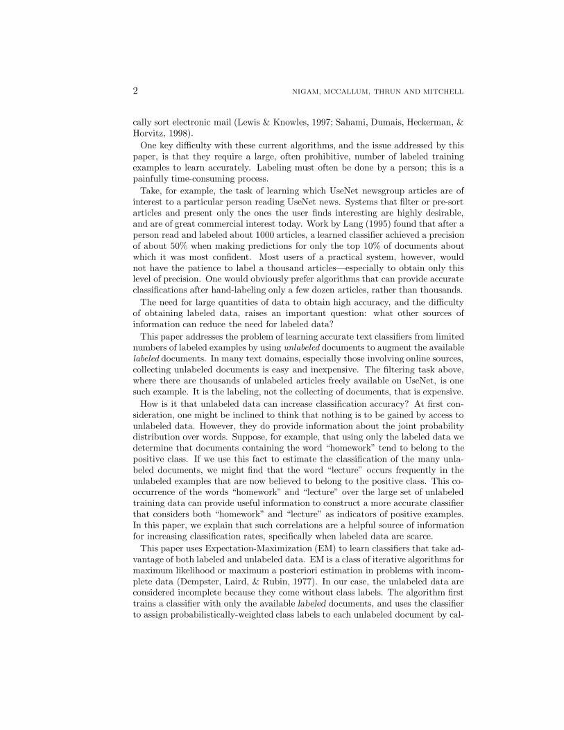
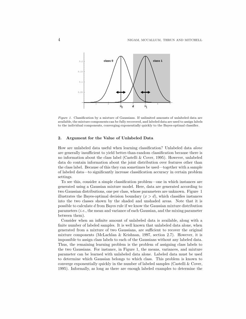
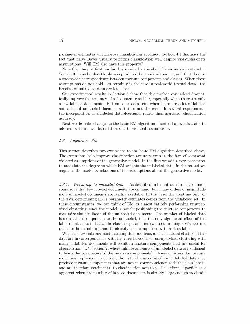
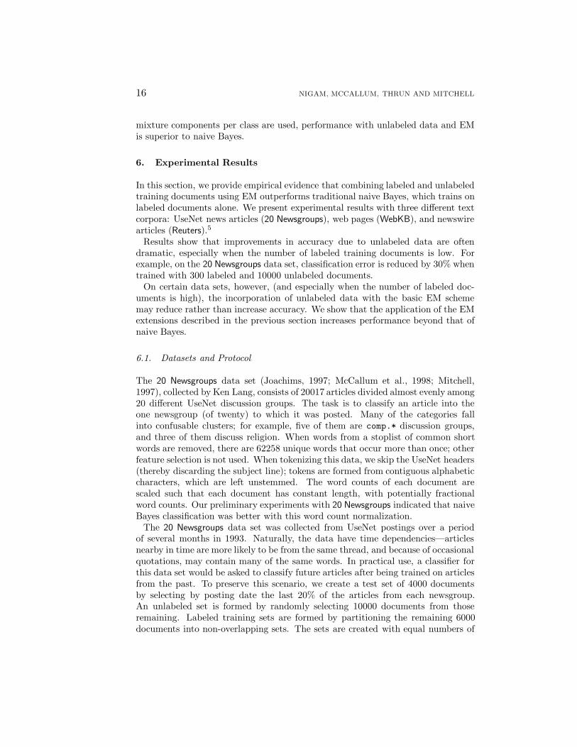
Figure 1. Classification by a mixture of Gaussians. If unlimited amounts of unlabeled data areavailable, the mixture components can be fully recovered, and labeled data are used to assign labelsto the individual components, converging exponentially quickly to the Bayes-optimal classifier.

2. Argument for the Value of Unlabeled Data

How are unlabeled data useful when learning classification? Unlabeled data aloneare generally insufficient to yield better-than-random classification because there isno information about the class label (Castelli & Cover, 1995). However, unlabeleddata do contain information about the joint distribution over features other thanthe class label. Because of this they can sometimes be used—together with a sampleof labeled data—to significantly increase classification accuracy in certain problemsettings.

To see this, consider a simple classification problem—one in which instances aregenerated using a Gaussian mixture model. Here, data are generated according totwo Gaussian distributions, one per class, whose parameters are unknown. Figure 1illustrates the Bayes-optimal decision boundary (x > d), which classifies instancesinto the two classes shown by the shaded and unshaded areas. Note that it ispossible to calculate d from Bayes rule if we know the Gaussian mixture distributionparameters (i.e., the mean and variance of each Gaussian, and the mixing parameterbetween them).

Consider when an infinite amount of unlabeled data is available, along with afinite number of labeled samples. It is well known that unlabeled data alone, whengenerated from a mixture of two Gaussians, are sufficient to recover the originalmixture components (McLachlan & Krishnan, 1997, section 2.7). However, it isimpossible to assign class labels to each of the Gaussians without any labeled data.Thus, the remaining learning problem is the problem of assigning class labels tothe two Gaussians. For instance, in Figure 1, the means, variances, and mixtureparameter can be learned with unlabeled data alone. Labeled data must be usedto determine which Gaussian belongs to which class. This problem is known toconverge exponentially quickly in the number of labeled samples (Castelli & Cover,1995). Informally, as long as there are enough labeled examples to determine the


class of each component, the parameter estimation can be done with unlabeled dataalone.

It is important to notice that this result depends on the critical assumption thatthe data indeed have been generated using the same parametric model as used inclassification, something that almost certainly is untrue in real-world domains suchas text classification. This raises the important empirical question as to what extentunlabeled data can be useful in practice in spite of the violated assumptions. In thefollowing sections we address this by describing in detail a parametric generativemodel for text classification and by presenting empirical results using this modelon real-world data.

3. The Probabilistic Framework

This section presents a probabilistic framework for characterizing the nature ofdocuments and classifiers. The framework defines a probabilistic generative modelfor the data, and embodies two assumptions about the generative process: (1) thedata are produced by a mixture model, and (2) there is a one-to-one correspondencebetween mixture components and classes.1 The naive Bayes text classifier we willdiscuss later falls into this framework, as does the example in Section 2.

In this setting, every document is generated according to a probability distributiondefined by a set of parameters, denoted θ. The probability distribution consists of amixture of components cj ∈ C = {c1, ..., c|C|}. Each component is parameterized bya disjoint subset of θ. A document, di, is created by first selecting a mixture com-ponent according to the mixture weights (or class prior probabilities), P(cj |θ), thenhaving this selected mixture component generate a document according to its ownparameters, with distribution P(di|cj; θ).2 Thus, we can characterize the likelihoodof document di with a sum of total probability over all mixture components:

P(di|θ) =|C|∑j=1

P(cj |θ)P(di|cj; θ). (1)

Each document has a class label. We assume that there is a one-to-one corre-spondence between mixture model components and classes, and thus (for the timebeing) use cj to indicate the jth mixture component as well as, the jth class. Theclass label for a particular document di is written yi. If document di was generatedby mixture component cj we say yi = cj. The class label may or may not be knownfor a given document.

4. Text Classification with Naive Bayes

This section presents naive Bayes—a well-known probabilistic classifier—and de-scribes its application to text. Naive Bayes is the foundation upon which we willlater build in order to incorporate unlabeled data.

The learning task in this section is to estimate the parameters of a generativemodel using labeled training data only. The algorithm uses the estimated param-


eters to classify new documents by calculating which class was most likely to havegenerated the given document.

4.1. The Generative Model

Naive Bayes assumes a particular probabilistic generative model for text. The modelis a specialization of the mixture model presented in the previous section, and thusalso makes the two assumptions discussed there. Additionally, naive Bayes makesword independence assumptions that allow the generative model to be characterizedwith a greatly reduced number of parameters. The rest of this subsection describesthe generative model more formally, giving a precise specification of the modelparameters, and deriving the probability that a particular document is generatedgiven its class label (Equation 4).

First let us introduce some notation to describe text. A document, di, is con-sidered to be an ordered list of word events, 〈wdi,1 , wdi,2, . . .〉. We write wdi,k forthe word wt in position k of document di, where wt is a word in the vocabularyV = 〈w1, w2, . . . , w|V |〉.

When a document is to be generated by a particular mixture component, cj, adocument length, |di|, is chosen independently of the component. (Note that thisassumes that document length is independent of class.3) Then, the selected mixturecomponent generates a word sequence of the specified length. We furthermoreassume it generates each word independently of the length.

Thus, we can expand the second term from Equation 1, and express the probabil-ity of a document given a mixture component in terms of its constituent features:the document length and the words in the document. Note that, in this generalsetting, the probability of a word event must be conditioned on all the words thatprecede it.

P(di|cj; θ) = P(〈wdi,1 , . . . , wdi,|di|〉|cj; θ) = P(|di|)|di|∏k=1

P(wdi,k |cj; θ;wdi,q , q < k) (2)

Next we make the standard naive Bayes assumption: that the words of a documentare generated independently of context, that is, independently of the other wordsin the same document given the class label. We further assume that the probabilityof a word is independent of its position within the document; thus, for example,the probability of seeing the word “homework” in the first position of a documentis the same as seeing it in any other position. We can express these assumptionsas:

P(wdi,k |cj; θ;wdi,q , q < k) = P(wdi,k |cj; θ). (3)

Combining these last two equations gives the naive Bayes expression for the prob-ability of a document given its class:

P(di|cj; θ) = P(|di|)|di|∏k=1

P(wdi,k |cj; θ). (4)


Thus the parameters of an individual mixture component are a multinomial dis-tribution over words, i.e. the collection of word probabilities, each written θwt |cj ,such that θwt |cj = P(wt|cj; θ), where t = {1, . . . , |V |} and

∑t P(wt|cj; θ) = 1. Since

we assume that for all classes, document length is identically distributed, it doesnot need to be parameterized for classification. The only other parameters of themodel are the mixture weights (class prior probabilities), written θcj , which indicatethe probabilities of selecting the different mixture components. Thus the completecollection of model parameters, θ, is a set of multinomials and prior probabilitiesover those multinomials: θ = {θwt|cj : wt ∈ V, cj ∈ C ; θcj : cj ∈ C}.

4.2. Training a Classifier

Learning a naive Bayes text classifier consists of estimating the parameters of thegenerative model by using a set of labeled training data, D = {d1, . . . , d|D|}. Thissubsection derives a method for calculating these estimates from the training data.

The estimate of θ is written θ. Naive Bayes uses the maximum a posterioriestimate, thus finding arg maxθ P(θ|D). This is the value of θ that is most probablegiven the evidence of the training data and a prior.

The parameter estimation formulae that result from this maximization are thefamiliar ratios of empirical counts. The estimated probability of a word given aclass, θwt|cj , is simply the number of times word wt occurs in the training data forclass cj , divided by the total number of word occurrences in the training data forthat class—where counts in both the numerator and denominator are augmentedwith “pseudo-counts” (one for each word) that come from the prior distributionover θ. The use of this type of prior is sometimes referred to as Laplace smooth-ing. Smoothing is necessary to prevent zero probabilities for infrequently occurringwords.

The word probability estimates θwt|cj are:

θwt|cj ≡ P(wt|cj; θ) =1 +

∑|D|i=1 N(wt, di)P(yi = cj|di)

|V |+∑|V |s=1

∑|D|i=1 N(ws, di)P(yi = cj|di)

, (5)

where N(wt, di) is the count of the number of times word wt occurs in documentdi and where P(yi = cj|di) ∈ {0, 1} as given by the class label.

The class prior probabilities, θcj , are estimated in the same manner, and alsoinvolve a ratio of counts with smoothing:

θcj ≡ P(cj |θ) =1 +

∑|D|i=1 P(yi = cj |di)|C|+ |D| . (6)

The derivation of these “ratios of counts” formulae comes directly from maxi-mum a posteriori parameter estimation, and will be appealed to again later whenderiving parameter estimation formulae for EM and augmented EM. Finding theθ that maximizes P(θ|D) is accomplished by first breaking this expression intotwo terms by Bayes’ rule: P(θ|D) ∝ P(D|θ)P(θ). The first term is calculated by


the product of all the document likelihoods (from Equation 1). The second term,the prior distribution over parameters, we represent by a Dirichlet distribution:P(θ) ∝

∏cj∈C

((θcj )α−1

∏wt∈V (θwt |cj)

α−1), where α is a parameter that effects

the strength of the prior, and is some constant greater than zero.4 In this paper, weset α = 2, which (with maximum a posteriori estimation) is equivalent to Laplacesmoothing. The whole expression is maximized by solving the system of partialderivatives of log(P(θ|D)), using Lagrange multipliers to enforce the constraintthat the word probabilities in a class must sum to one. This maximization yieldsthe ratio of counts seen above.

4.3. Using a Classifier

Given estimates of these parameters calculated from the training documents ac-cording to Equations 5 and 6, it is possible to turn the generative model backwardsand calculate the probability that a particular mixture component generated agiven document. We derive this by an application of Bayes’ rule, and then bysubstitutions using Equations 1 and 4:

P(yi = cj|di; θ) =P(cj |θ)P(di|cj; θ)

P(di|θ)

=P(cj |θ)

∏|di|k=1 P(wdi,k |cj; θ)∑|C|

r=1 P(cr |θ)∏|di|k=1 P(wdi,k |cr; θ)

. (7)

If the task is to classify a test document di into a single class, then the class withthe highest posterior probability, arg maxj P(yi = cj |di; θ), is selected.

4.4. Discussion

Note that all four assumptions about the generation of text documents (mixturemodel, one-to-one correspondence between mixture components and classes, wordindependence, and document length distribution) are violated in real-world textdata. Documents are often mixtures of multiple topics. Words within a documentare not independent of each other—grammar and topicality make this so.

Despite these violations, empirically the Naive Bayes classifier does a good job ofclassifying text documents (Lewis & Ringuette, 1994; Craven et al., 1998; Yang &Pederson, 1997; Joachims, 1997; McCallum, Rosenfeld, Mitchell, & Ng, 1998). Thisobservation is explained in part by the fact that classification estimation is only afunction of the sign (in binary classification) of the function estimation (Domingos& Pazzani, 1997; Friedman, 1997). The word independence assumption causesnaive Bayes to give extreme (almost 0 or 1) class probability estimates. However,these estimates can still be poor while classification accuracy remains high.

The above formulation of naive Bayes uses a generative model that accounts forthe number of times a word appears in a document. It is a multinomial (or in lan-


guage modeling terms, “unigram”) model, where the classifier is a mixture of multi-nomials (McCallum & Nigam, 1998). This formulation has been used by numerouspractitioners of naive Bayes text classification (Lewis & Gale, 1994; Joachims, 1997;Li & Yamanishi, 1997; Mitchell, 1997; McCallum et al., 1998; Lewis, 1998). How-ever, there is another formulation of naive Bayes text classification that instead usesa generative model and document representation in which each word in the vocab-ulary is a binary feature, and is modeled by a mixture of multi-variate Bernoullis(Robertson & Sparck-Jones, 1976; Lewis, 1992; Larkey & Croft, 1996; Koller & Sa-hami, 1997). Empirical comparisons show that the multinomial formulation yieldsclassifiers with consistently higher accuracy (McCallum & Nigam, 1998).

5. Incorporating Unlabeled Data with EM

We now proceed to the main topic of this paper: how unlabeled data can be usedto improve a text classifier. When naive Bayes is given just a small set of labeledtraining data, classification accuracy will suffer because variance in the parameterestimates of the generative model will be high. However, by augmenting this smallset with a large set of unlabeled data, and combining the two sets with EM, we canimprove the parameter estimates.

EM is a class of iterative algorithms for maximum likelihood or maximum aposteriori estimation in problems with incomplete data (Dempster et al., 1977). Inour case, the unlabeled data are considered incomplete because they come withoutclass labels.

Applying EM to naive Bayes is quite straightforward. First, the naive Bayesparameters, θ, are estimated from just the labeled documents. Then, the classifier isused to assign probabilistically-weighted class labels to each unlabeled document bycalculating expectations of the missing class labels, P(cj |di; θ). Next, new classifierparameters, θ, are estimated using all the documents—both the originally and newlylabeled. These last two steps are iterated until θ does not change. As shown byDempster et al. (1977), at each iteration, this process is guaranteed to find modelparameters that have equal or higher likelihood than at the previous iteration.

This section describes EM and our extensions within the probabilistic frameworkof naive Bayes text classification.

5.1. Basic EM

We are given a set of training documents D and the task is to build a classifier in theform of the previous section. However, unlike previously, in this section we assumethat only some subset of the documents di ∈ Dl come with class labels yi ∈ C, andfor the rest of the documents, in subset Du, the class labels are unknown. Thus wehave a disjoint partitioning of D, such that D = Dl ∪ Du.

As in Section 4.2, learning a classifier is approached as calculating a maximuma posteriori estimate of θ, i.e. arg maxθ P(θ)P(D|θ). Consider the second term ofthe maximization, the probability of all the training data, D. The probability of allthe data is simply the product over all the documents, because each document is


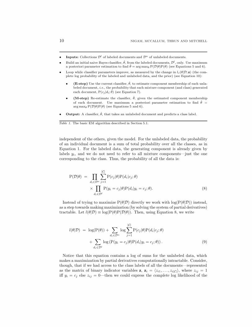
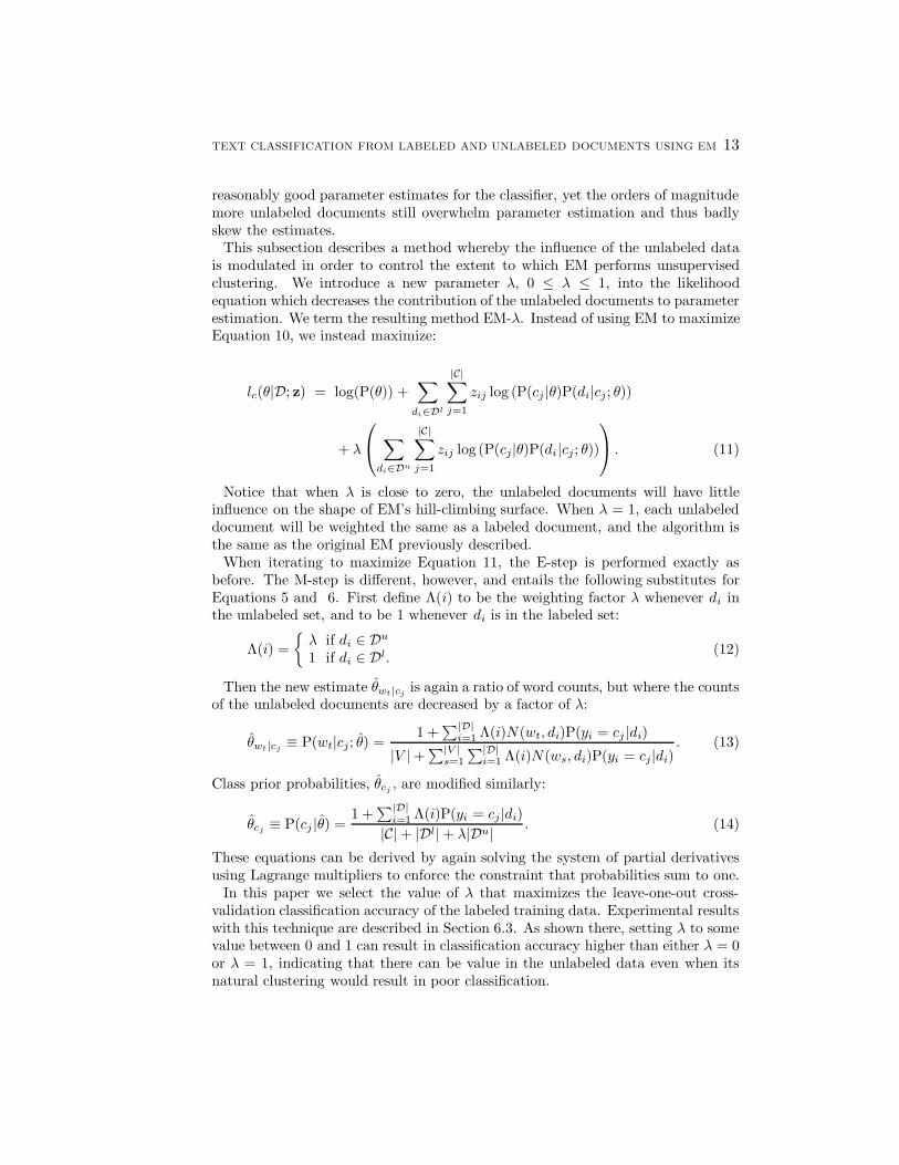
• Inputs: Collections Dl of labeled documents and Du of unlabeled documents.

• Build an initial naive Bayes classifier, θ, from the labeled documents,Dl, only. Use maximuma posteriori parameter estimation to find θ = arg maxθ P(D|θ)P(θ) (see Equations 5 and 6).

• Loop while classifier parameters improve, as measured by the change in lc(θ|D; z) (the com-plete log probability of the labeled and unlabeled data, and the prior) (see Equation 10):

• (E-step) Use the current classifier, θ, to estimate component membership of each unla-beled document, i.e., the probability that each mixture component (and class) generated

each document, P(cj |di; θ) (see Equation 7).

• (M-step) Re-estimate the classifier, θ, given the estimated component membership

of each document. Use maximum a posteriori parameter estimation to find θ =arg maxθ P(D|θ)P(θ) (see Equations 5 and 6).

• Output: A classifier, θ, that takes an unlabeled document and predicts a class label.

Table 1. The basic EM algorithm described in Section 5.1.

independent of the others, given the model. For the unlabeled data, the probabilityof an individual document is a sum of total probability over all the classes, as inEquation 1. For the labeled data, the generating component is already given bylabels yi, and we do not need to refer to all mixture components—just the onecorresponding to the class. Thus, the probability of all the data is:

P(D|θ) =∏

di∈Du

|C|∑j=1

P(cj|θ)P(di|cj; θ)

×∏di∈Dl

P(yi = cj |θ)P(di|yi = cj; θ). (8)

Instead of trying to maximize P(θ|D) directly we work with log(P(θ|D)) instead,as a step towards making maximization (by solving the system of partial derivatives)tractable. Let l(θ|D) ≡ log(P(θ)P(D|θ)). Then, using Equation 8, we write

l(θ|D) = log(P(θ)) +∑di∈Du

log|C|∑j=1

P(cj |θ)P(di|cj; θ)

+∑di∈Dl

log (P(yi = cj |θ)P(di|yi = cj; θ)) . (9)

Notice that this equation contains a log of sums for the unlabeled data, whichmakes a maximization by partial derivatives computationally intractable. Consider,though, that if we had access to the class labels of all the documents—representedas the matrix of binary indicator variables z, zi = 〈zi1, . . . , zi|C|〉, where zij = 1iff yi = cj else zij = 0—then we could express the complete log likelihood of the


parameters, lc(θ|D, z), without a log of sums, because only one term inside the sumwould be non-zero.

lc(θ|D; z) = log(P(θ)) +∑di∈D

|C|∑j=1

zij log (P(cj |θ)P(di|cj; θ)) (10)

If we replace zij by its expected value according to the current model, thenEquation 10 bounds from below the incomplete log likelihood from Equation 9. Thiscan be shown by an application of Jensen’s inequality (e.g. E[log(X)] ≥ log(E[X])).As a result one can find a locally maximum θ by a hill climbing procedure. Thiswas formalized as the Expectation-Maximization (EM) algorithm by Dempster et al.(1977).

The iterative hill climbing procedure alternately recomputes the expected valueof z and the maximum a posteriori parameters given the expected value of z, E[z].Note that for the labeled documents zi is already known. It must, however, beestimated for the unlabeled documents. Let z(k) and θ(k) denote the estimates forz and θ at iteration k. Then, the algorithm finds a local maximum of l(θ|D) byiterating the following two steps:

• E-step: Set z(k+1) = E[z|D; θ(k)].

• M-step: Set θ(k+1) = arg maxθ P(θ|D; z(k+1)).

In practice, the E-step corresponds to calculating probabilistic labels P(cj |di; θ)for the unlabeled documents by using the current estimate of the parameters, θ, andEquation 7. The M-step, maximizing the complete likelihood equation, correspondsto calculating a new maximum a posteriori estimate for the parameters, θ, usingthe current estimates for P(cj |di; θ), and Equations 5 and 6.

Our iteration process is initialized with a “priming” M-step, in which only thelabeled documents are used to estimate the classifier parameters, θ, as in Equa-tions 5 and 6. Then the cycle begins with an E-step that uses this classifier toprobabilistically label the unlabeled documents for the first time.

The algorithm iterates over the E- and M-steps until it converges to a point whereθ does not change from one iteration to the next. Algorithmically, we determinethat convergence has occurred by observing a below-threshold change in the log-probability of the parameters (Equation 10), which is the height of the surface onwhich EM is hill-climbing.

Table 1 gives an outline of the basic EM algorithm from this section.

5.2. Discussion

In summary, EM finds a θ that locally maximizes the likelihood of its parame-ters given all the data—both the labeled and the unlabeled. It provides a methodwhereby unlabeled data can augment limited labeled data and contribute to param-eter estimation. An interesting empirical question is whether these higher likelihood


parameter estimates will improve classification accuracy. Section 4.4 discusses thefact that naive Bayes usually performs classification well despite violations of itsassumptions. Will EM also have this property?

Note that the justifications for this approach depend on the assumptions stated inSection 3, namely, that the data is produced by a mixture model, and that there isa one-to-one correspondence between mixture components and classes. When theseassumptions do not hold—as certainly is the case in real-world textual data—thebenefits of unlabeled data are less clear.

Our experimental results in Section 6 show that this method can indeed dramat-ically improve the accuracy of a document classifier, especially when there are onlya few labeled documents. But on some data sets, when there are a lot of labeledand a lot of unlabeled documents, this is not the case. In several experiments,the incorporation of unlabeled data decreases, rather than increases, classificationaccuracy.

Next we describe changes to the basic EM algorithm described above that aim toaddress performance degradation due to violated assumptions.

5.3. Augmented EM

This section describes two extensions to the basic EM algorithm described above.The extensions help improve classification accuracy even in the face of somewhatviolated assumptions of the generative model. In the first we add a new parameterto modulate the degree to which EM weights the unlabeled data; in the second weaugment the model to relax one of the assumptions about the generative model.

5.3.1. Weighting the unlabeled data. As described in the introduction, a commonscenario is that few labeled documents are on hand, but many orders of magnitudemore unlabeled documents are readily available. In this case, the great majority ofthe data determining EM’s parameter estimates comes from the unlabeled set. Inthese circumstances, we can think of EM as almost entirely performing unsuper-vised clustering, since the model is mostly positioning the mixture components tomaximize the likelihood of the unlabeled documents. The number of labeled datais so small in comparison to the unlabeled, that the only significant effect of thelabeled data is to initialize the classifier parameters (i.e. determining EM’s startingpoint for hill climbing), and to identify each component with a class label.

When the two mixture model assumptions are true, and the natural clusters of thedata are in correspondence with the class labels, then unsupervised clustering withmany unlabeled documents will result in mixture components that are useful forclassification (c.f. Section 2, where infinite amounts of unlabeled data are sufficientto learn the parameters of the mixture components). However, when the mixturemodel assumptions are not true, the natural clustering of the unlabeled data mayproduce mixture components that are not in correspondence with the class labels,and are therefore detrimental to classification accuracy. This effect is particularlyapparent when the number of labeled documents is already large enough to obtain


reasonably good parameter estimates for the classifier, yet the orders of magnitudemore unlabeled documents still overwhelm parameter estimation and thus badlyskew the estimates.

This subsection describes a method whereby the influence of the unlabeled datais modulated in order to control the extent to which EM performs unsupervisedclustering. We introduce a new parameter λ, 0 ≤ λ ≤ 1, into the likelihoodequation which decreases the contribution of the unlabeled documents to parameterestimation. We term the resulting method EM-λ. Instead of using EM to maximizeEquation 10, we instead maximize:

lc(θ|D; z) = log(P(θ)) +∑di∈Dl

|C|∑j=1

zij log (P(cj |θ)P(di|cj; θ))

+ λ

∑di∈Du

|C|∑j=1

zij log (P(cj|θ)P(di|cj; θ))

. (11)

Notice that when λ is close to zero, the unlabeled documents will have littleinfluence on the shape of EM’s hill-climbing surface. When λ = 1, each unlabeleddocument will be weighted the same as a labeled document, and the algorithm isthe same as the original EM previously described.

When iterating to maximize Equation 11, the E-step is performed exactly asbefore. The M-step is different, however, and entails the following substitutes forEquations 5 and 6. First define Λ(i) to be the weighting factor λ whenever di inthe unlabeled set, and to be 1 whenever di is in the labeled set:

Λ(i) ={λ if di ∈ Du1 if di ∈ Dl.

(12)

Then the new estimate θwt|cj is again a ratio of word counts, but where the countsof the unlabeled documents are decreased by a factor of λ:

θwt|cj ≡ P(wt|cj; θ) =1 +

∑|D|i=1 Λ(i)N(wt, di)P(yi = cj |di)

|V |+∑|V |s=1

∑|D|i=1 Λ(i)N(ws, di)P(yi = cj|di)

. (13)

Class prior probabilities, θcj , are modified similarly:

θcj ≡ P(cj |θ) =1 +

∑|D|i=1 Λ(i)P(yi = cj|di)|C|+ |Dl|+ λ|Du| . (14)

These equations can be derived by again solving the system of partial derivativesusing Lagrange multipliers to enforce the constraint that probabilities sum to one.

In this paper we select the value of λ that maximizes the leave-one-out cross-validation classification accuracy of the labeled training data. Experimental resultswith this technique are described in Section 6.3. As shown there, setting λ to somevalue between 0 and 1 can result in classification accuracy higher than either λ = 0or λ = 1, indicating that there can be value in the unlabeled data even when itsnatural clustering would result in poor classification.


5.3.2. Multiple mixture components per class. The EM-λ technique describedabove addresses violated mixture model assumptions by reducing the effect of thoseviolated assumptions on parameter estimation. An alternative approach is to at-tack the problem head-on by removing or weakening a restrictive assumption. Thissubsection takes exactly this approach by relaxing the assumption of a one-to-onecorrespondence between mixture components and classes. We replace it with aless restrictive assumption: a many-to-one correspondence between mixture com-ponents and classes.

For textual data, this corresponds to saying that a class may be comprised ofseveral different sub-topics, each best captured with a different word distribution.Furthermore, using multiple mixture components per class can capture some depen-dencies between words. For example, consider a sports class consisting of documentsabout both hockey and baseball. In these documents, the words “ice” and “puck”are likely to co-occur, and the words “bat” and “base” are likely to co-occur. How-ever, these dependencies cannot be captured by a single multinomial distributionover words in the sports class. On the other hand, with multiple mixture compo-nents per class, one multinomial can cover the hockey sub-topic, and another thebaseball sub-topic—thus more accurately capturing the co-occurrence patterns ofthe above four words.

For some or all of the classes we now allow multiple multinomial mixture com-ponents. Note that as a result, there are now “missing values” for the labeled aswell as the unlabeled documents—it is unknown which mixture component, amongthose covering the given label, is responsible for generating a particular labeled doc-ument. Parameter estimation will still be performed with EM except that, for eachlabeled document, we must now estimate which mixture component the documentcame from.

Let us introduce the following notation for separating mixture components fromclasses. Instead of using cj to denote both a class and its corresponding mixturecomponent, we will now write ta for the ath class (“topic”), and cj will continueto denote the jth mixture component. We write P(ta|cj; θ) ∈ {0, 1} for the pre-determined, deterministic, many-to-one mapping between mixture components andclasses.

Parameter estimation is again done with EM. The M-step is the same as ba-sic EM, building maximum a posteriori parameter estimates for the multinomialof each component. In the E-step, unlabeled documents are treated as before,calculating probabilistically-weighted mixture component membership, P(cj |di; θ).For labeled documents, the previous P(cj |di; θ) ∈ {0, 1} that was considered tobe fixed by the class label is now allowed to vary between 0 and 1 for mixturecomponents assigned to that document’s class. Thus, the algorithm also calculatesprobabilistically-weighted mixture component membership for the labeled docu-ments. Note, however, that all P(cj |di; θ), for which P(yi = ta|cj; θ) is zero, areclamped at zero, and the rest are normalized to sum to one.

Multiple mixture components for the same class are initialized by randomlyspreading the labeled training data across the mixture components matching theappropriate class label. That is, components are initialized by performing a ran-


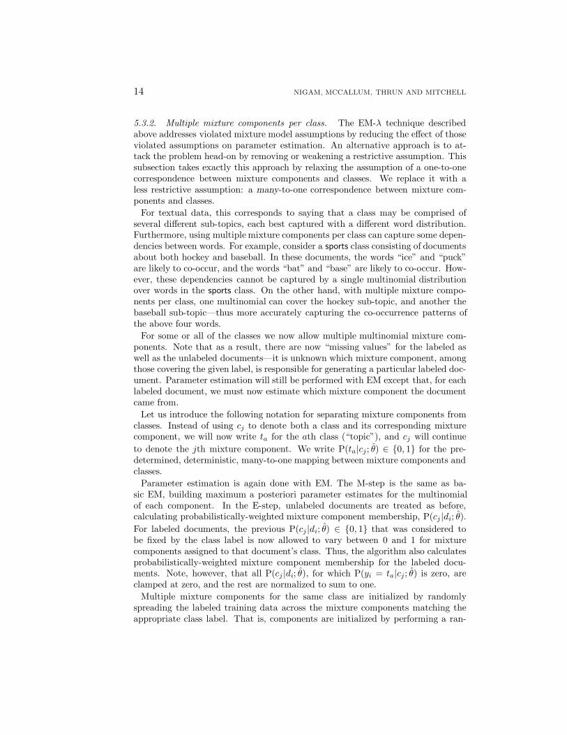
• Inputs: Collections Dl of labeled documents and Du of unlabeled documents.

• [Weighted only]: Set the discount factor of the unlabeled data, λ, by cross-validation (seeSections 6.1 and 6.3).

• [Multiple only]: Set the number of mixture components per class by cross-validation (seeSections 6.1 and 6.4).

• [Multiple only]: For each labeled document, randomly assign P(cj |di; θ) for mixture com-ponents that correspond to the document’s class label, to initialize each mixture component.

• Build an initial naive Bayes classifier, θ, from the labeled documents only. Use maximum aposteriori parameter estimation to find θ = arg maxθ P(D|θ)P(θ) (see Equations 5 and 6).

• Loop while classifier parameters improve (0.05 < ∆lc(θ|D; z), the change in complete logprobability of the labeled and unlabeled data, and the prior) (see Equation 10):

• (E-step) Use the current classifier, θ, to estimate the component membership of eachdocument, i.e. the probability that each mixture component generated each document,P(cj |di; θ) (see Equation 7).

[Multiple only]: Restrict the membership probability estimates of labeled documentsto be zero for components associated with other classes, and renormalize.

• (M-step) Re-estimate the classifier, θ, given the estimated component membership

of each document. Use maximum a posteriori parameter estimation to find θ =arg maxθ P(D|θ)P(θ) (see Equations 5 and 6).

[Weighted only]: When counting events for parameter estimation, word and documentcounts from unlabeled documents are reduced by a factor λ (see Equations 13 and 14).

• Output: A classifier, θ, that takes an unlabeled document and predicts a class label.

Table 2. The Algorithm described in this paper, and used to generate the experimental resultsin Section 6. The algorithm enhancements for EM-λ that vary the contribution of the unlabeleddata (Section 5.3.1) are indicated by [Weighted only]. The optional use of multiple mixturecomponents per class (Section 5.3.2) is indicated by [Multiple only]. Unmarked paragraphs arecommon to all variations of the algorithm.

domized E-step in which P(cj |di; θ) is sampled from a uniform distribution overmixture components for which P(ta = yi|cj; θ) is one.

When there are multiple mixture components per class, classification becomes amatter of probabilistically “classifying” documents into the mixture components,and then summing the mixture component probabilities into class probabilities:

P(ta|di; θ) =∑cj

P(ta|cj; θ)P(cj|θ)

∏|di|k=1 P(wdi,k |cj; θ)∑|C|

r=1 P(cr |θ)∏|di|k=1 P(wdi,k |cr; θ)

. (15)

In this paper, we select the number of mixture components per class by cross-validation. Table 2 gives an outline of the EM algorithm with the extensions of thisand the previous section.

Experimental results from this technique are described in Section 6.4. As shownthere, when the data are not naturally modeled by a single component per class,the use of unlabeled data with EM degrades performance. However, when multiple


mixture components per class are used, performance with unlabeled data and EMis superior to naive Bayes.

6. Experimental Results

In this section, we provide empirical evidence that combining labeled and unlabeledtraining documents using EM outperforms traditional naive Bayes, which trains onlabeled documents alone. We present experimental results with three different textcorpora: UseNet news articles (20 Newsgroups), web pages (WebKB), and newswirearticles (Reuters).5

Results show that improvements in accuracy due to unlabeled data are oftendramatic, especially when the number of labeled training documents is low. Forexample, on the 20 Newsgroups data set, classification error is reduced by 30% whentrained with 300 labeled and 10000 unlabeled documents.

On certain data sets, however, (and especially when the number of labeled doc-uments is high), the incorporation of unlabeled data with the basic EM schememay reduce rather than increase accuracy. We show that the application of the EMextensions described in the previous section increases performance beyond that ofnaive Bayes.

6.1. Datasets and Protocol

The 20 Newsgroups data set (Joachims, 1997; McCallum et al., 1998; Mitchell,1997), collected by Ken Lang, consists of 20017 articles divided almost evenly among20 different UseNet discussion groups. The task is to classify an article into theone newsgroup (of twenty) to which it was posted. Many of the categories fallinto confusable clusters; for example, five of them are comp.* discussion groups,and three of them discuss religion. When words from a stoplist of common shortwords are removed, there are 62258 unique words that occur more than once; otherfeature selection is not used. When tokenizing this data, we skip the UseNet headers(thereby discarding the subject line); tokens are formed from contiguous alphabeticcharacters, which are left unstemmed. The word counts of each document arescaled such that each document has constant length, with potentially fractionalword counts. Our preliminary experiments with 20 Newsgroups indicated that naiveBayes classification was better with this word count normalization.

The 20 Newsgroups data set was collected from UseNet postings over a periodof several months in 1993. Naturally, the data have time dependencies—articlesnearby in time are more likely to be from the same thread, and because of occasionalquotations, may contain many of the same words. In practical use, a classifier forthis data set would be asked to classify future articles after being trained on articlesfrom the past. To preserve this scenario, we create a test set of 4000 documentsby selecting by posting date the last 20% of the articles from each newsgroup.An unlabeled set is formed by randomly selecting 10000 documents from thoseremaining. Labeled training sets are formed by partitioning the remaining 6000documents into non-overlapping sets. The sets are created with equal numbers of


documents per class. For experiments with different labeled set sizes, we create upto ten sets per size; obviously, fewer sets are possible for experiments with labeledsets containing more than 600 documents. The use of each non-overlapping trainingset comprises a new trial of the given experiment. Results are reported as averagesover all trials of the experiment.

The WebKB data set (Craven et al., 1998) contains 8145 web pages gathered fromuniversity computer science departments. The collection includes the entirety offour departments, and additionally, an assortment of pages from other universities.The pages are divided into seven categories: student, faculty, staff, course, project,department and other. In this paper, we use the four most populous non-othercategories: student, faculty, course and project—all together containing 4199 pages.The task is to classify a web page into the appropriate one of the four categories.For consistency with previous studies with this data set (Craven et al., 1998), whentokenizing the WebKB data, numbers were converted into a time or a phone numbertoken, if appropriate, or otherwise a sequence-of-length-n token.

We did not use stemming or a stoplist; we found that using a stoplist actually hurtperformance. For example, “my” is an excellent indicator of a student homepageand is the fourth-ranked word by information gain. We limit the vocabulary tothe 300 most informative words, as measured by average mutual information withthe class variable. This feature selection method is commonly used for text (Yang& Pederson, 1997; Koller & Sahami, 1997; Joachims, 1997). We selected thisvocabulary size by running leave-one-out cross-validation on the training data tooptimize classification accuracy.

The WebKB data set was collected as part of an effort to create a crawler thatexplores previously unseen computer science departments and classifies web pagesinto a knowledge-base ontology. To mimic the crawler’s intended use, and to avoidreporting performance based on idiosyncrasies particular to a single department,we test using a leave-one-university-out approach. That is, we create four test sets,each containing all the pages from one of the four complete computer science de-partments. For each test set, an unlabeled set of 2500 pages is formed by randomlyselecting from the remaining web pages. Non-overlapping training sets are formedby the same method as in 20 Newsgroups. Also as before, results are reported asaverages over all trials that share the same number of labeled training documents.

The Reuters 21578 Distribution 1.0 data set consists of 12902 articles and 90 topiccategories from the Reuters newswire. Following several other studies (Joachims,1998; Liere & Tadepalli, 1997) we build binary classifiers for each of the ten mostpopulous classes to identify the news topic. We use all the words inside the <TEXT>tags, including the title and the dateline, except that we remove the REUTER and&# tags that occur at the top and bottom of every document. We use a stoplist,but do not stem.

In Reuters, classifiers for different categories perform best with widely varyingvocabulary sizes (which are chosen by average mutual information with the classvariable). This variance in optimal vocabulary size is unsurprising. As previouslynoted (Joachims, 1997), categories like “wheat” and “corn” are known for a strongcorrespondence between a small set of words (like their title words) and the cate-


gories, while categories like “acq” are known for more complex characteristics. Thecategories with narrow definitions attain best classification with small vocabularies,while those with a broader definition require a large vocabulary. The vocabularysize for each Reuters trial is selected by optimizing accuracy as measured by leave-one-out cross-validation on the labeled training set.

As with the 20 Newsgroups data set, there are time dependencies in Reuters. Thestandard ‘ModApte’ train/test split divides the articles by time, such that the later3299 documents form the test set, and the earlier 9603 are available for training.In our experiments, 7000 documents from this training set are randomly selectedto form the unlabeled set. From the remaining training documents, we randomlyselect up to ten non-overlapping training sets of ten positively labeled documentsand 40 negatively labeled documents, as previously described for the other twodata sets. We use non-uniform number of labelings across the classes because thenegative class is much more frequent than the positive class in all of the binaryReuters classification tasks.

Results on Reuters are reported as precision-recall breakeven points, a standardinformation retrieval measure for binary classification. Accuracy is not a goodperformance metric here because very high accuracy can be achieved by alwayspredicting the negative class. The task on this data set is less like classificationthan it is like filtering—find the few positive examples from a large sea of negativeexamples. Recall and precision capture the inherent duality of this task, and aredefined as:

Recall =# of correct positive predictions

# of positive examples(16)

Precision =# of correct positive predictions

# of positive predictions. (17)

The classifier can achieve a trade-off between precision and recall by adjusting thedecision boundary between the positive and negative class away from its previousdefault of P(cj |di; θ) = 0.5. The precision-recall breakeven point is defined as theprecision and recall value at which the two are equal (e.g. Joachims, 1998).

The algorithm used for experiments with EM is described in Table 2.In this section, when leave-one-out cross-validation is performed in conjunction

with EM, we make one simplification for computational efficiency. We first run EMto convergence with all the training data, and then subtract the word counts of eachlabeled document in turn before testing that document. Thus, when performingcross-validation for a specific combination of parameter settings, only one run ofEM is required instead of one run of EM per labeled example. Note, however, thatthere are still some residual effects of the held-out document.

The computational complexity of EM, however, is not prohibitive. Each iterationrequires classifying the training documents (E-step), and building a new classifier(M-step). In our experiments, EM usually converges after about 10 iterations. Thewall-clock time to read the document-word matrix from disk, build an EM modelby iterating to convergence, and classify the test documents is less than one minute


0%

10%

20%

30%

40%

50%

60%

70%

80%

90%

100%

10 20 50 100 200 500 1000 2000 5000

Acc

urac

y

Number of Labeled Documents

10000 unlabeled documentsNo unlabeled documents

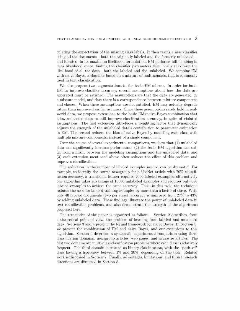
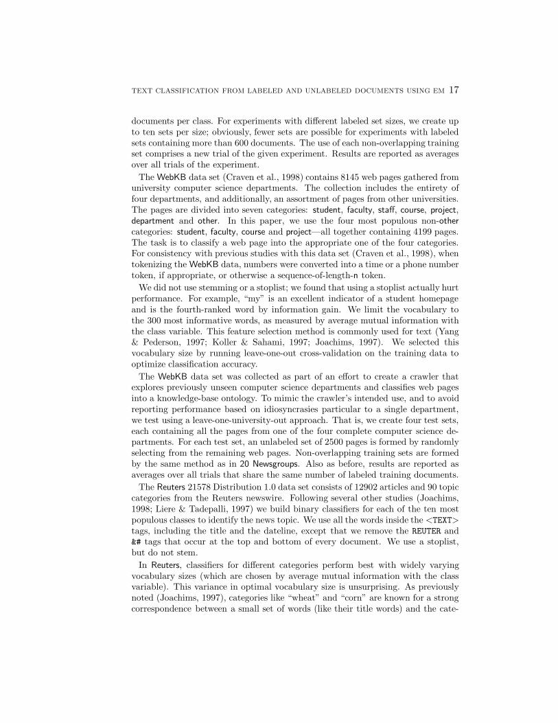
Figure 2. Classification accuracy on the 20 Newsgroups data set, both with and without 10,000unlabeled documents. With small amounts of training data, using EM yields more accurateclassifiers. With large amounts of labeled training data, accurate parameter estimates can beobtained without the use of unlabeled data, and the two methods begin to converge.

for the WebKB data set, and less than 15 minutes for 20 Newsgroups. The 20Newsgroups data set takes longer because it has more documents and more wordsin the vocabulary.

6.2. EM with Unlabeled Data Increases Accuracy

We first consider the use of basic EM to incorporate information from unlabeleddocuments. Figure 2 shows the effect of using basic EM with unlabeled data onthe 20 Newsgroups data set. The vertical axis indicates average classifier accuracyon test sets, and the horizontal axis indicates the amount of labeled training dataon a log scale. We vary the amount of labeled training data, and compare theclassification accuracy of traditional naive Bayes (no unlabeled data) with an EMlearner that has access to 10000 unlabeled documents.

EM performs significantly better. For example, with 300 labeled documents (15documents per class), naive Bayes reaches 52% accuracy while EM achieves 66%.This represents a 30% reduction in classification error. Note that EM also performswell even with a very small number of labeled documents; with only 20 documents (asingle labeled document per class), naive Bayes obtains 20%, EM 35%. As expected,when there is a lot of labeled data, and the naive Bayes learning curve is close toa plateau, having unlabeled data does not help nearly as much, because there isalready enough labeled data to accurately estimate the classifier parameters. With5500 labeled documents (275 per class), classification accuracy increases from 76%to 78%. Each of these results is statistically significant (p < 0.05).6

These results demonstrate that EM finds parameter estimates that improve clas-sification accuracy and reduce the need for labeled training examples. For example,to reach 70% classification accuracy, naive Bayes requires 2000 labeled examples,while EM requires only 600 labeled examples to achieve the same accuracy.


0%

10%

20%

30%

40%

50%

60%

70%

80%

90%

100%

0 1000 3000 5000 7000 9000 11000 13000

Acc

urac

y

Number of Unlabeled Documents

3000 labeled documents600 labeled documents300 labeled documents140 labeled documents40 labeled documents

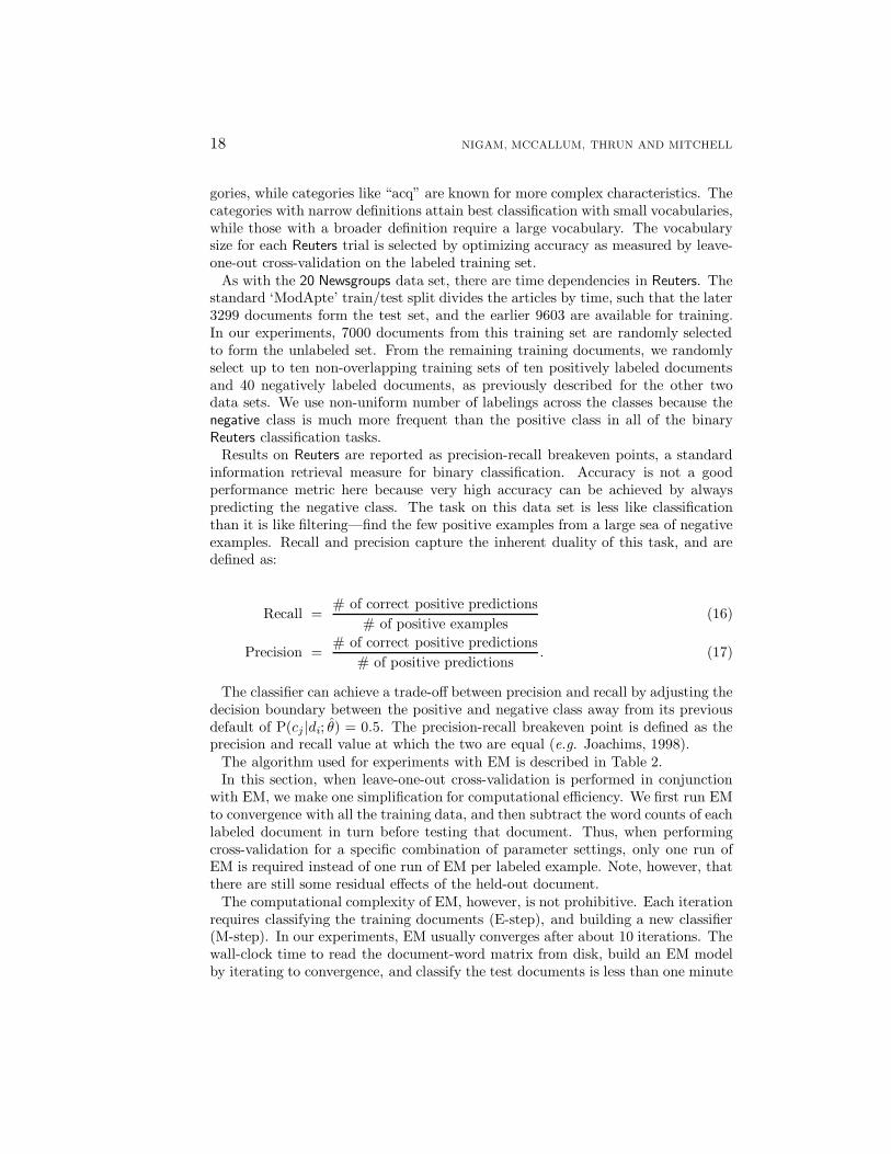
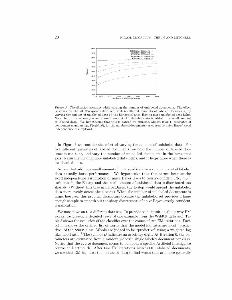
Figure 3. Classification accuracy while varying the number of unlabeled documents. The effectis shown on the 20 Newsgroups data set, with 5 different amounts of labeled documents, byvarying the amount of unlabeled data on the horizontal axis. Having more unlabeled data helps.Note the dip in accuracy when a small amount of unlabeled data is added to a small amountof labeled data. We hypothesize that this is caused by extreme, almost 0 or 1, estimates ofcomponent membership, P(cj |di, θ), for the unlabeled documents (as caused by naive Bayes’ wordindependence assumption).

In Figure 3 we consider the effect of varying the amount of unlabeled data. Forfive different quantities of labeled documents, we hold the number of labeled doc-uments constant, and vary the number of unlabeled documents in the horizontalaxis. Naturally, having more unlabeled data helps, and it helps more when there isless labeled data.

Notice that adding a small amount of unlabeled data to a small amount of labeleddata actually hurts performance. We hypothesize that this occurs because theword independence assumption of naive Bayes leads to overly-confident P(cj |di, θ)estimates in the E-step, and the small amount of unlabeled data is distributed toosharply. (Without this bias in naive Bayes, the E-step would spread the unlabeleddata more evenly across the classes.) When the number of unlabeled documents islarge, however, this problem disappears because the unlabeled set provides a largeenough sample to smooth out the sharp discreteness of naive Bayes’ overly-confidentclassification.

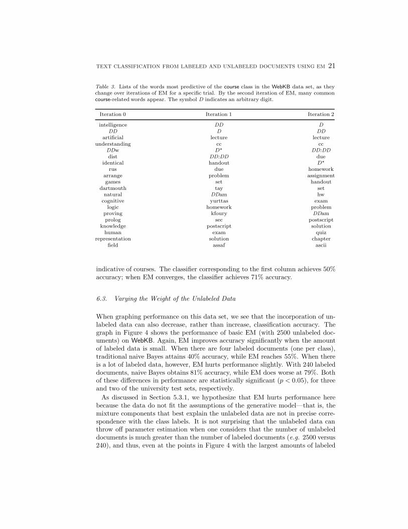
We now move on to a different data set. To provide some intuition about why EMworks, we present a detailed trace of one example from the WebKB data set. Ta-ble 3 shows the evolution of the classifier over the course of two EM iterations. Eachcolumn shows the ordered list of words that the model indicates are most “predic-tive” of the course class. Words are judged to be “predictive” using a weighted loglikelihood ratio.7 The symbol D indicates an arbitrary digit. At Iteration 0, the pa-rameters are estimated from a randomly-chosen single labeled document per class.Notice that the course document seems to be about a specific Artificial Intelligencecourse at Dartmouth. After two EM iterations with 2500 unlabeled documents,we see that EM has used the unlabeled data to find words that are more generally


Table 3. Lists of the words most predictive of the course class in the WebKB data set, as theychange over iterations of EM for a specific trial. By the second iteration of EM, many commoncourse-related words appear. The symbol D indicates an arbitrary digit.

Iteration 0 Iteration 1 Iteration 2

intelligence DD DDD D DD

artificial lecture lectureunderstanding cc cc

DDw D? DD:DDdist DD:DD due

identical handout D?

rus due homeworkarrange problem assignmentgames set handout

dartmouth tay setnatural DDam hw

cognitive yurttas examlogic homework problem

proving kfoury DDamprolog sec postscript

knowledge postscript solutionhuman exam quiz

representation solution chapterfield assaf ascii

indicative of courses. The classifier corresponding to the first column achieves 50%accuracy; when EM converges, the classifier achieves 71% accuracy.

6.3. Varying the Weight of the Unlabeled Data

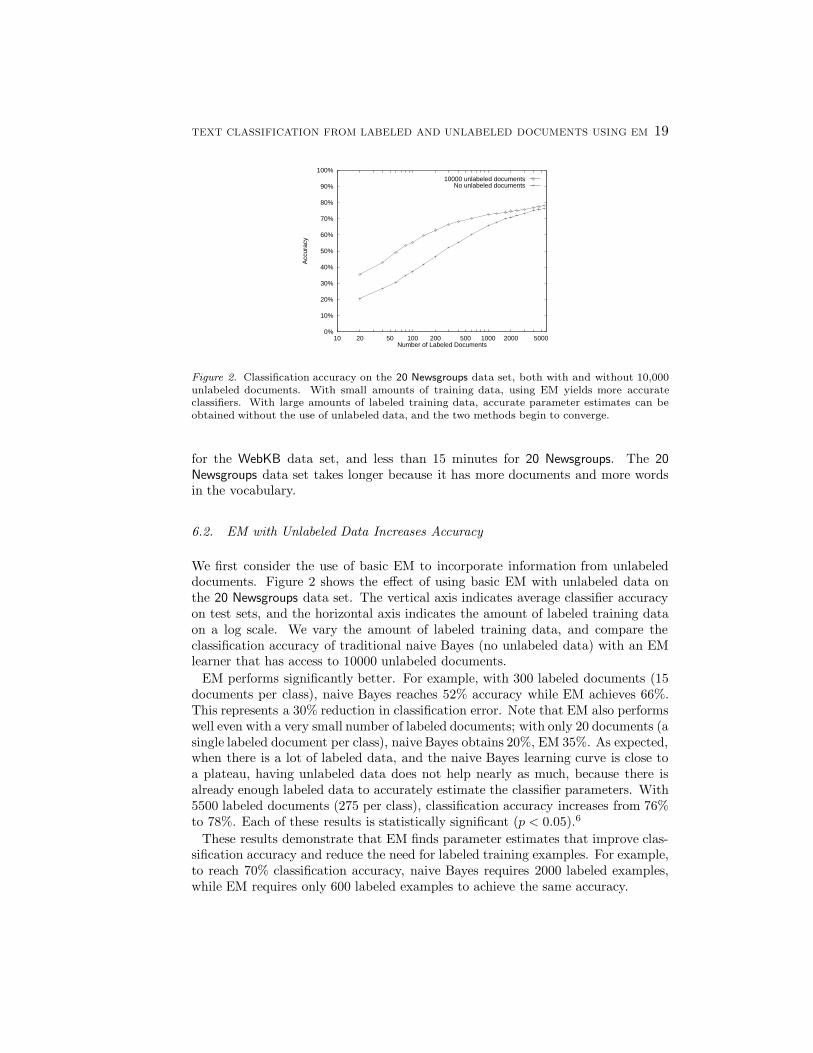
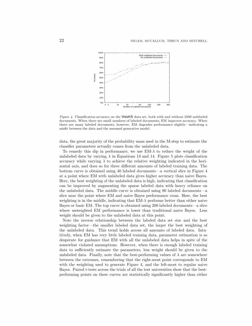
When graphing performance on this data set, we see that the incorporation of un-labeled data can also decrease, rather than increase, classification accuracy. Thegraph in Figure 4 shows the performance of basic EM (with 2500 unlabeled doc-uments) on WebKB. Again, EM improves accuracy significantly when the amountof labeled data is small. When there are four labeled documents (one per class),traditional naive Bayes attains 40% accuracy, while EM reaches 55%. When thereis a lot of labeled data, however, EM hurts performance slightly. With 240 labeleddocuments, naive Bayes obtains 81% accuracy, while EM does worse at 79%. Bothof these differences in performance are statistically significant (p < 0.05), for threeand two of the university test sets, respectively.

As discussed in Section 5.3.1, we hypothesize that EM hurts performance herebecause the data do not fit the assumptions of the generative model—that is, themixture components that best explain the unlabeled data are not in precise corre-spondence with the class labels. It is not surprising that the unlabeled data canthrow off parameter estimation when one considers that the number of unlabeleddocuments is much greater than the number of labeled documents (e.g. 2500 versus240), and thus, even at the points in Figure 4 with the largest amounts of labeled


0%

10%

20%

30%

40%

50%

60%

70%

80%

90%

100%

4 5 10 20 50 100 200 400

Acc

urac

y


2500 unlabeled documentsNo unlabeled documents

Figure 4. Classification accuracy on the WebKB data set, both with and without 2500 unlabeleddocuments. When there are small numbers of labeled documents, EM improves accuracy. Whenthere are many labeled documents, however, EM degrades performance slightly—indicating amisfit between the data and the assumed generative model.

data, the great majority of the probability mass used in the M-step to estimate theclassifier parameters actually comes from the unlabeled data.

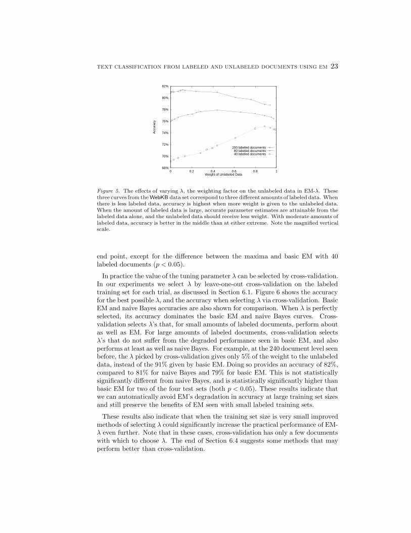
To remedy this dip in performance, we use EM-λ to reduce the weight of theunlabeled data by varying λ in Equations 13 and 14. Figure 5 plots classificationaccuracy while varying λ to achieve the relative weighting indicated in the hori-zontal axis, and does so for three different amounts of labeled training data. Thebottom curve is obtained using 40 labeled documents—a vertical slice in Figure 4at a point where EM with unlabeled data gives higher accuracy than naive Bayes.Here, the best weighting of the unlabeled data is high, indicating that classificationcan be improved by augmenting the sparse labeled data with heavy reliance onthe unlabeled data. The middle curve is obtained using 80 labeled documents—aslice near the point where EM and naive Bayes performance cross. Here, the bestweighting is in the middle, indicating that EM-λ performs better than either naiveBayes or basic EM. The top curve is obtained using 200 labeled documents—a slicewhere unweighted EM performance is lower than traditional naive Bayes. Lessweight should be given to the unlabeled data at this point.

Note the inverse relationship between the labeled data set size and the bestweighting factor—the smaller labeled data set, the larger the best weighting ofthe unlabeled data. This trend holds across all amounts of labeled data. Intu-itively, when EM has very little labeled training data, parameter estimation is sodesperate for guidance that EM with all the unlabeled data helps in spite of thesomewhat violated assumptions. However, when there is enough labeled trainingdata to sufficiently estimate the parameters, less weight should be given to theunlabeled data. Finally, note that the best-performing values of λ are somewherebetween the extremes, remembering that the right-most point corresponds to EMwith the weighting used to generate Figure 4, and the left-most to regular naiveBayes. Paired t-tests across the trials of all the test universities show that the best-performing points on these curves are statistically significantly higher than either


68%

70%

72%

74%

76%

78%

80%

82%

0 0.2 0.4 0.6 0.8 1

Acc

urac

y

Weight of Unlabeled Data

200 labeled documents80 labeled documents40 labeled documents

Figure 5. The effects of varying λ, the weighting factor on the unlabeled data in EM-λ. Thesethree curves from the WebKB data set correspond to three different amounts of labeled data. Whenthere is less labeled data, accuracy is highest when more weight is given to the unlabeled data.When the amount of labeled data is large, accurate parameter estimates are attainable from thelabeled data alone, and the unlabeled data should receive less weight. With moderate amounts oflabeled data, accuracy is better in the middle than at either extreme. Note the magnified verticalscale.

end point, except for the difference between the maxima and basic EM with 40labeled documents (p < 0.05).

In practice the value of the tuning parameter λ can be selected by cross-validation.In our experiments we select λ by leave-one-out cross-validation on the labeledtraining set for each trial, as discussed in Section 6.1. Figure 6 shows the accuracyfor the best possible λ, and the accuracy when selecting λ via cross-validation. BasicEM and naive Bayes accuracies are also shown for comparison. When λ is perfectlyselected, its accuracy dominates the basic EM and naive Bayes curves. Cross-validation selects λ’s that, for small amounts of labeled documents, perform aboutas well as EM. For large amounts of labeled documents, cross-validation selectsλ’s that do not suffer from the degraded performance seen in basic EM, and alsoperforms at least as well as naive Bayes. For example, at the 240 document level seenbefore, the λ picked by cross-validation gives only 5% of the weight to the unlabeleddata, instead of the 91% given by basic EM. Doing so provides an accuracy of 82%,compared to 81% for naive Bayes and 79% for basic EM. This is not statisticallysignificantly different from naive Bayes, and is statistically significantly higher thanbasic EM for two of the four test sets (both p < 0.05). These results indicate thatwe can automatically avoid EM’s degradation in accuracy at large training set sizesand still preserve the benefits of EM seen with small labeled training sets.

These results also indicate that when the training set size is very small improvedmethods of selecting λ could significantly increase the practical performance of EM-λ even further. Note that in these cases, cross-validation has only a few documentswith which to choose λ. The end of Section 6.4 suggests some methods that mayperform better than cross-validation.


40%

45%

50%

55%

60%

65%

70%

75%

80%

85%

4 5 10 20 50 100 200 400

Acc

urac

y


2500 unlabeled documents with best EM-lambda2500 unlabeled documents with CV EM-lambda

2500 unlabeled documents with basic EMNo unlabeled documents

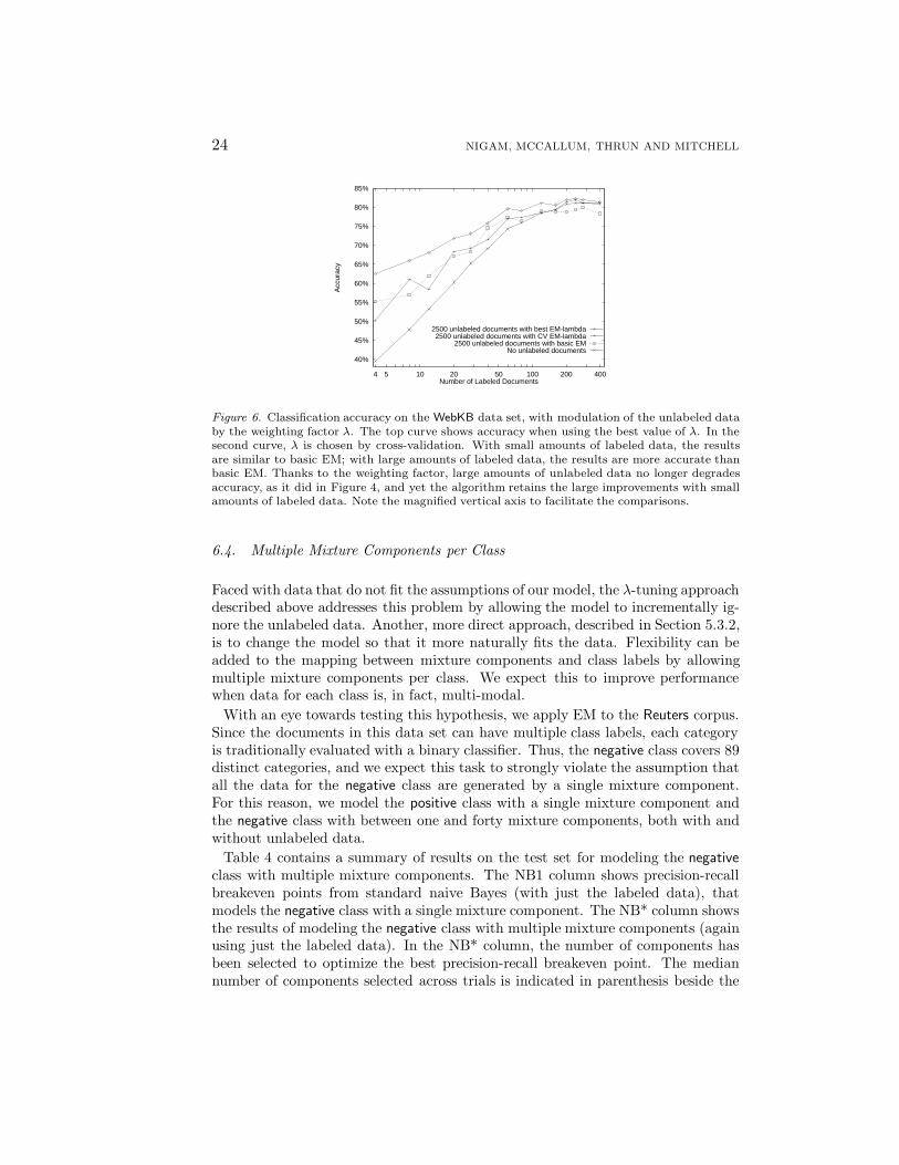
Figure 6. Classification accuracy on the WebKB data set, with modulation of the unlabeled databy the weighting factor λ. The top curve shows accuracy when using the best value of λ. In thesecond curve, λ is chosen by cross-validation. With small amounts of labeled data, the resultsare similar to basic EM; with large amounts of labeled data, the results are more accurate thanbasic EM. Thanks to the weighting factor, large amounts of unlabeled data no longer degradesaccuracy, as it did in Figure 4, and yet the algorithm retains the large improvements with smallamounts of labeled data. Note the magnified vertical axis to facilitate the comparisons.

6.4. Multiple Mixture Components per Class

Faced with data that do not fit the assumptions of our model, the λ-tuning approachdescribed above addresses this problem by allowing the model to incrementally ig-nore the unlabeled data. Another, more direct approach, described in Section 5.3.2,is to change the model so that it more naturally fits the data. Flexibility can beadded to the mapping between mixture components and class labels by allowingmultiple mixture components per class. We expect this to improve performancewhen data for each class is, in fact, multi-modal.

With an eye towards testing this hypothesis, we apply EM to the Reuters corpus.Since the documents in this data set can have multiple class labels, each categoryis traditionally evaluated with a binary classifier. Thus, the negative class covers 89distinct categories, and we expect this task to strongly violate the assumption thatall the data for the negative class are generated by a single mixture component.For this reason, we model the positive class with a single mixture component andthe negative class with between one and forty mixture components, both with andwithout unlabeled data.

Table 4 contains a summary of results on the test set for modeling the negativeclass with multiple mixture components. The NB1 column shows precision-recallbreakeven points from standard naive Bayes (with just the labeled data), thatmodels the negative class with a single mixture component. The NB* column showsthe results of modeling the negative class with multiple mixture components (againusing just the labeled data). In the NB* column, the number of components hasbeen selected to optimize the best precision-recall breakeven point. The mediannumber of components selected across trials is indicated in parenthesis beside the


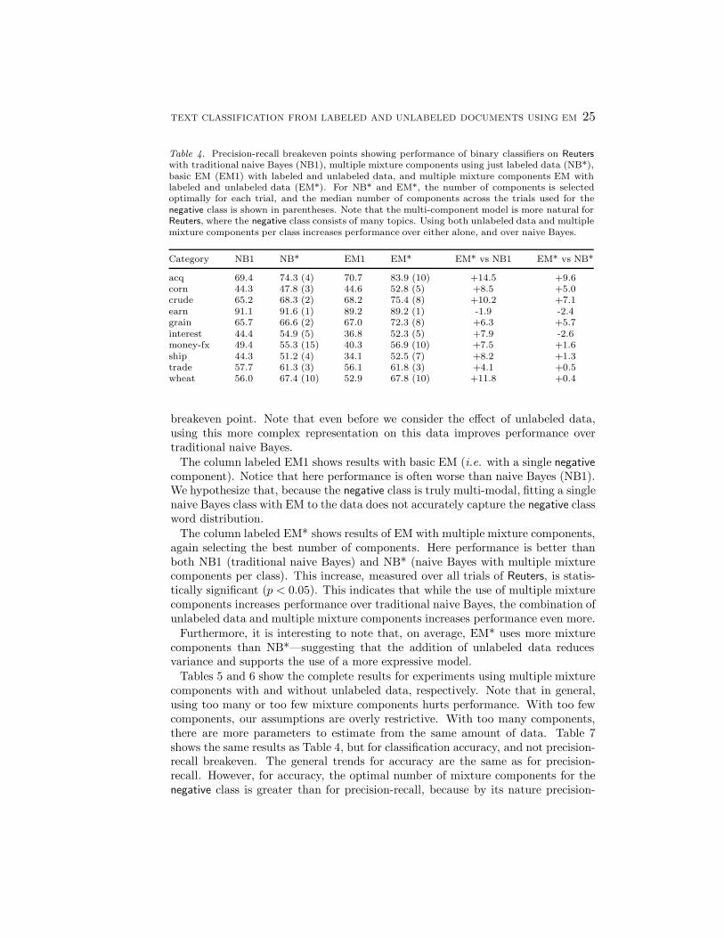
Table 4. Precision-recall breakeven points showing performance of binary classifiers on Reuterswith traditional naive Bayes (NB1), multiple mixture components using just labeled data (NB*),basic EM (EM1) with labeled and unlabeled data, and multiple mixture components EM withlabeled and unlabeled data (EM*). For NB* and EM*, the number of components is selectedoptimally for each trial, and the median number of components across the trials used for thenegative class is shown in parentheses. Note that the multi-component model is more natural forReuters, where the negative class consists of many topics. Using both unlabeled data and multiplemixture components per class increases performance over either alone, and over naive Bayes.

Category NB1 NB* EM1 EM* EM* vs NB1 EM* vs NB*

acq 69.4 74.3 (4) 70.7 83.9 (10) +14.5 +9.6corn 44.3 47.8 (3) 44.6 52.8 (5) +8.5 +5.0crude 65.2 68.3 (2) 68.2 75.4 (8) +10.2 +7.1earn 91.1 91.6 (1) 89.2 89.2 (1) -1.9 -2.4grain 65.7 66.6 (2) 67.0 72.3 (8) +6.3 +5.7interest 44.4 54.9 (5) 36.8 52.3 (5) +7.9 -2.6money-fx 49.4 55.3 (15) 40.3 56.9 (10) +7.5 +1.6ship 44.3 51.2 (4) 34.1 52.5 (7) +8.2 +1.3trade 57.7 61.3 (3) 56.1 61.8 (3) +4.1 +0.5wheat 56.0 67.4 (10) 52.9 67.8 (10) +11.8 +0.4

breakeven point. Note that even before we consider the effect of unlabeled data,using this more complex representation on this data improves performance overtraditional naive Bayes.

The column labeled EM1 shows results with basic EM (i.e. with a single negativecomponent). Notice that here performance is often worse than naive Bayes (NB1).We hypothesize that, because the negative class is truly multi-modal, fitting a singlenaive Bayes class with EM to the data does not accurately capture the negative classword distribution.

The column labeled EM* shows results of EM with multiple mixture components,again selecting the best number of components. Here performance is better thanboth NB1 (traditional naive Bayes) and NB* (naive Bayes with multiple mixturecomponents per class). This increase, measured over all trials of Reuters, is statis-tically significant (p < 0.05). This indicates that while the use of multiple mixturecomponents increases performance over traditional naive Bayes, the combination ofunlabeled data and multiple mixture components increases performance even more.

Furthermore, it is interesting to note that, on average, EM* uses more mixturecomponents than NB*—suggesting that the addition of unlabeled data reducesvariance and supports the use of a more expressive model.

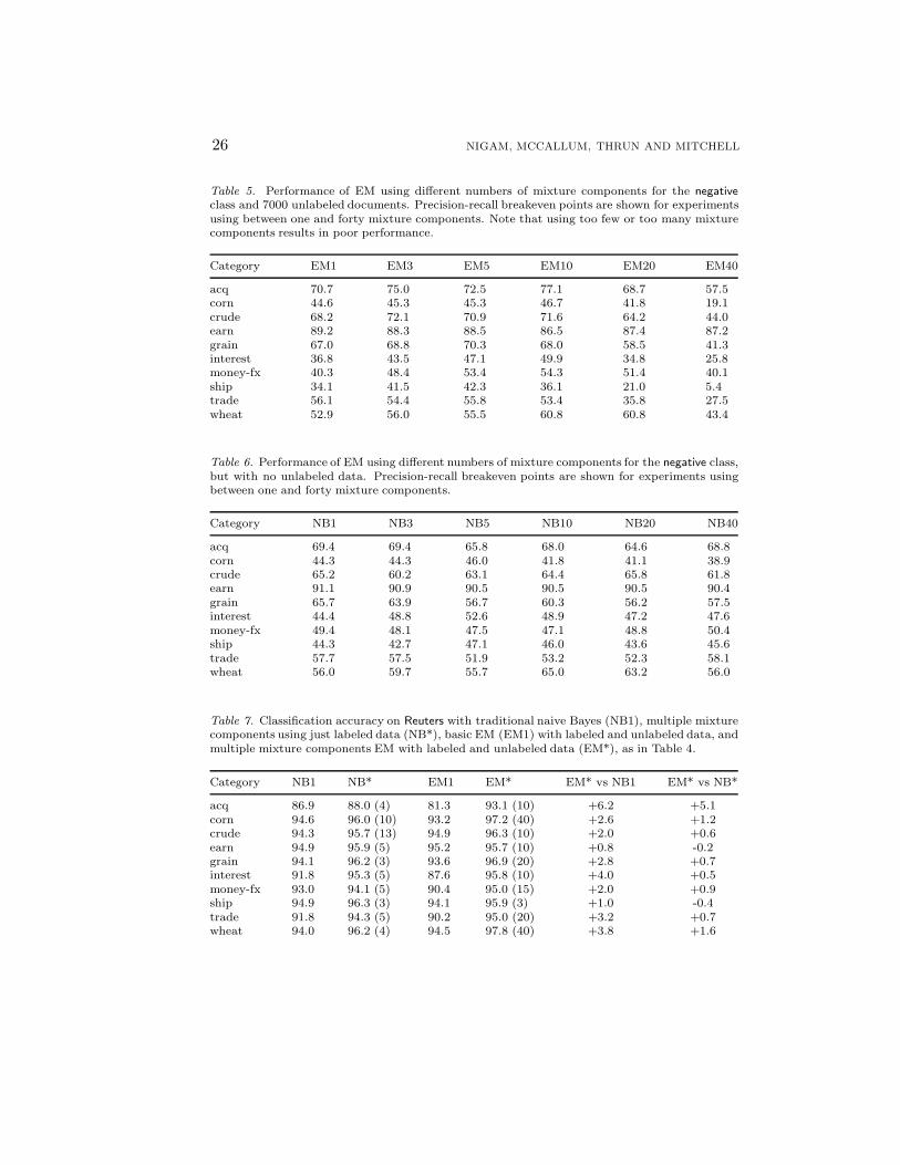
Tables 5 and 6 show the complete results for experiments using multiple mixturecomponents with and without unlabeled data, respectively. Note that in general,using too many or too few mixture components hurts performance. With too fewcomponents, our assumptions are overly restrictive. With too many components,there are more parameters to estimate from the same amount of data. Table 7shows the same results as Table 4, but for classification accuracy, and not precision-recall breakeven. The general trends for accuracy are the same as for precision-recall. However, for accuracy, the optimal number of mixture components for thenegative class is greater than for precision-recall, because by its nature precision-


Table 5. Performance of EM using different numbers of mixture components for the negativeclass and 7000 unlabeled documents. Precision-recall breakeven points are shown for experimentsusing between one and forty mixture components. Note that using too few or too many mixturecomponents results in poor performance.

Category EM1 EM3 EM5 EM10 EM20 EM40

acq 70.7 75.0 72.5 77.1 68.7 57.5corn 44.6 45.3 45.3 46.7 41.8 19.1crude 68.2 72.1 70.9 71.6 64.2 44.0earn 89.2 88.3 88.5 86.5 87.4 87.2grain 67.0 68.8 70.3 68.0 58.5 41.3interest 36.8 43.5 47.1 49.9 34.8 25.8money-fx 40.3 48.4 53.4 54.3 51.4 40.1ship 34.1 41.5 42.3 36.1 21.0 5.4trade 56.1 54.4 55.8 53.4 35.8 27.5wheat 52.9 56.0 55.5 60.8 60.8 43.4

Table 6. Performance of EM using different numbers of mixture components for the negative class,but with no unlabeled data. Precision-recall breakeven points are shown for experiments usingbetween one and forty mixture components.

Category NB1 NB3 NB5 NB10 NB20 NB40

acq 69.4 69.4 65.8 68.0 64.6 68.8corn 44.3 44.3 46.0 41.8 41.1 38.9crude 65.2 60.2 63.1 64.4 65.8 61.8earn 91.1 90.9 90.5 90.5 90.5 90.4grain 65.7 63.9 56.7 60.3 56.2 57.5interest 44.4 48.8 52.6 48.9 47.2 47.6money-fx 49.4 48.1 47.5 47.1 48.8 50.4ship 44.3 42.7 47.1 46.0 43.6 45.6trade 57.7 57.5 51.9 53.2 52.3 58.1wheat 56.0 59.7 55.7 65.0 63.2 56.0

Table 7. Classification accuracy on Reuters with traditional naive Bayes (NB1), multiple mixturecomponents using just labeled data (NB*), basic EM (EM1) with labeled and unlabeled data, andmultiple mixture components EM with labeled and unlabeled data (EM*), as in Table 4.

Category NB1 NB* EM1 EM* EM* vs NB1 EM* vs NB*

acq 86.9 88.0 (4) 81.3 93.1 (10) +6.2 +5.1corn 94.6 96.0 (10) 93.2 97.2 (40) +2.6 +1.2crude 94.3 95.7 (13) 94.9 96.3 (10) +2.0 +0.6earn 94.9 95.9 (5) 95.2 95.7 (10) +0.8 -0.2grain 94.1 96.2 (3) 93.6 96.9 (20) +2.8 +0.7interest 91.8 95.3 (5) 87.6 95.8 (10) +4.0 +0.5money-fx 93.0 94.1 (5) 90.4 95.0 (15) +2.0 +0.9ship 94.9 96.3 (3) 94.1 95.9 (3) +1.0 -0.4trade 91.8 94.3 (5) 90.2 95.0 (20) +3.2 +0.7wheat 94.0 96.2 (4) 94.5 97.8 (40) +3.8 +1.6


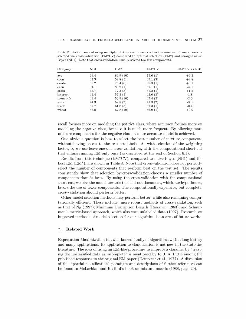
Table 8. Performance of using multiple mixture components when the number of components isselected via cross-validation (EM*CV) compared to optimal selection (EM*) and straight naiveBayes (NB1). Note that cross-validation usually selects too few components.

Category NB1 EM* EM*CV EM*CV vs NB1

acq 69.4 83.9 (10) 75.6 (1) +6.2corn 44.3 52.8 (5) 47.1 (3) +2.8crude 65.2 75.4 (8) 68.3 (1) +3.1earn 91.1 89.2 (1) 87.1 (1) -4.0grain 65.7 72.3 (8) 67.2 (1) +1.5interest 44.4 52.3 (5) 42.6 (3) -1.8money-fx 49.4 56.9 (10) 47.4 (2) -2.0ship 44.3 52.5 (7) 41.3 (2) -3.0trade 57.7 61.8 (3) 57.3 (1) -0.4wheat 56.0 67.8 (10) 56.9 (1) +0.9

recall focuses more on modeling the positive class, where accuracy focuses more onmodeling the negative class, because it is much more frequent. By allowing moremixture components for the negative class, a more accurate model is achieved.

One obvious question is how to select the best number of mixture componentswithout having access to the test set labels. As with selection of the weightingfactor, λ, we use leave-one-out cross-validation, with the computational short-cutthat entails running EM only once (as described at the end of Section 6.1).

Results from this technique (EM*CV), compared to naive Bayes (NB1) and thebest EM (EM*), are shown in Table 8. Note that cross-validation does not perfectlyselect the number of components that perform best on the test set. The resultsconsistently show that selection by cross-validation chooses a smaller number ofcomponents than is best. By using the cross-validation with the computationalshort-cut, we bias the model towards the held-out document, which, we hypothesize,favors the use of fewer components. The computationally expensive, but complete,cross-validation should perform better.

Other model selection methods may perform better, while also remaining compu-tationally efficient. These include: more robust methods of cross-validation, suchas that of Ng (1997); Minimum Description Length (Rissanen, 1983); and Schuur-man’s metric-based approach, which also uses unlabeled data (1997). Research onimproved methods of model selection for our algorithm is an area of future work.

7. Related Work

Expectation-Maximization is a well-known family of algorithms with a long historyand many applications. Its application to classification is not new in the statisticsliterature. The idea of using an EM-like procedure to improve a classifier by “treat-ing the unclassified data as incomplete” is mentioned by R. J. A. Little among thepublished responses to the original EM paper (Dempster et al., 1977). A discussionof this “partial classification” paradigm and descriptions of further references canbe found in McLachlan and Basford’s book on mixture models (1988, page 29).


Two recent studies in the machine learning literature have used EM to combinelabeled and unlabeled data for classification (Miller & Uyar, 1997; Shahshahani& Landgrebe, 1994). Instead of naive Bayes, Shahshahani and Landgrebe use amixture of Gaussians; Miller and Uyar use Mixtures of Experts. They demonstrateexperimental results on non-text data sets with up to 40 features. In contrast, ourtextual data sets have three orders of magnitude more features, which, we hypoth-esize, exacerbate violations of the independence and mixture model assumptions.

Shahshahani and Landgrebe (1994) also theoretically investigate the utility ofunlabeled data in supervised learning, with quite different results. They analyzethe convergence rate under the assumption that unbiased estimators are availablefor θ, for both the labeled and the unlabeled data. Their bounds, which are basedon Fisher information gain, show a linear (instead of exponential) value of labeledversus unlabeled data. Unfortunately, their analysis assumes that unlabeled dataalone is sufficient to estimate both parameter vectors; thus, they assume that thetarget concept can be recovered without any target labels. This assumption is un-realistic. As shown by Castelli and Cover (1995), unlabeled data does not improvethe classification results in the absence of labeled data.

Our work is an example of applying EM to fill in missing values—the missingvalues are the class labels of the unlabeled training examples. Work by Ghahramaniand Jordan (1994) is another example in the machine learning literature of usingEM with mixture models to fill in missing values. Whereas we focus on data wherethe class labels are missing, they focus on data where features other than the classlabels are missing. The AutoClass project (Cheeseman & Stutz, 1996) investigatesthe combination of Expectation-Maximization with a naive Bayes generative model.The emphasis of their research is the discovery of novel clustering for unsupervisedlearning over unlabeled data.

Our use of multiple mixture components per class is an example of using mixturesto improve modeling of probability density functions. Jaakkola and Jordan (1998)provide a general discussion of using mixtures to improve mean field approximations(of which naive Bayes is an example).

Another paradigm that reduces the need for labeled training examples is activelearning. In this scenario, the algorithm repeatedly selects an unlabeled example,asks a human labeler for its true class label, and rebuilds its classifier. Active learn-ing algorithms differ in their methods of selecting the unlabeled example. Threesuch examples applied to text are “Query By Committee” (Dagan & Engelson, 1995;Liere & Tadepalli, 1997), relevance sampling and uncertainty sampling (Lewis &Gale, 1994; Lewis, 1995).

Recent work by some of the authors combines active learning with Expectation-Maximization (McCallum & Nigam, 1998). EM is applied to the unlabeled docu-ments both to help inform the algorithm’s choice of documents for labeling requests,and also to boost accuracy using the documents that remain unlabeled (as in thispaper). Experimental results show that the combination of active learning and EMrequires only slightly more than half as many labeled training examples to achievethe same accuracy as either active learning or EM alone.


Another effort to use unlabeled data in support of supervised learning is the workon co-training by Blum and Mitchell (1998). They consider a particular subclass oflearning problems distinct from the problems addressed in this paper. In particular,they consider problems where a target function f(x) is to be learned, and where theattributes describing each instance x can be partitioned into two sets such that eachis sufficient to calculate f . This redundancy in the attributes describing x allowslearning two distinct classifiers, then using them to train one another over unlabeleddata. They present experimental results showing the success of this approach ona web page classification task, as well as a proof that under certain conditions thetarget function can be PAC learned given an initial weak classifier and unlabeleddata only.

A variety of statistical techniques other than naive Bayes have been applied totext classification, including Support Vector Machines (Joachims, 1998), k nearestneighbor (Yang, 1994, 1999), TFIDF/Rocchio (Salton, 1991; Rocchio, 1971), ex-ponential gradient and covering algorithms (Cohen & Singer, 1996). We use naiveBayes in this paper because is has a strong probabilistic foundation for Expectation-Maximization, and is more efficient for large data sets. Furthermore, the thrust ofthis paper is to straightforwardly demonstrate the value of unlabeled data; a similarapproach could apply unlabeled data to more complex classifiers.

8. Summary and Conclusions

This paper has presented a family of algorithms that address the question of whenand how unlabeled data may be used to supplement scarce labeled data, espe-cially when learning to classify text documents. This is an important question intext learning, because of the high cost of hand-labeling data and because of theavailability of large volumes of unlabeled data. We have presented an algorithmthat takes advantage of it and experimental results that show significant improve-ments by using unlabeled documents for training classifiers in three real-world textclassification tasks.

When our assumptions of data generation are correct, basic EM can effectivelyincorporate information from unlabeled data. However, the full complexity of real-world text data cannot be completely captured by known statistical models. Itis interesting then, to consider the performance of a classifier based on generativemodels that make incorrect assumptions about the data. In such cases, when thedata is inconsistent with the assumptions of the model, our method for adjustingthe relative contribution of the unlabeled data (EM-λ) prevents the unlabeled datafrom degrading classification accuracy.

In another augmentation to the basic EM scheme, we study the effect of multiplemixture components per class. This is an effort to relax the assumptions of themodel, and make the generative model better match the data. Experimental re-sults show improvements in classification, and suggest the exploration of even morecomplex mixture models that would correspond even better to textual data dis-tributions. These results also recommend a study of improvements to the current


cross-validation methods for selecting both the unlabeled data weight λ and thenumber of mixture components per class.

We believe that our algorithm and others using unlabeled data require a closermatch between the data and the generative model than those using labeled dataalone. If the intended target concept and model differ from the actual distributionof the data too strongly, then the use of unlabeled data will hurt instead of helpperformance. In future work we intend to make a closer theoretical and empiri-cal study of the tradeoffs between the use of unlabeled data and inherent modelinadequacies.

We also see several other interesting directions for future work with unlabeleddata. Two other task formulations could also benefit from using EM: (1) activelearning could use an explicit model of unlabeled data and incorporate EM, bothto improve selection of examples for which to request a label and to improve classifi-cation accuracy using the examples that remain unlabeled at the end; initial studyin this area has already begun (McCallum & Nigam, 1998); (2) an incrementallearning algorithm that re-trains throughout the testing phase could use the unla-beled test data received early in the testing phase in order to improve performanceon the later test data.

Furthermore, other problem domains share some similarities with text domains,and also have limited, expensive labeled data, but abundant and inexpensive un-labeled data. Robotics, vision, and information extraction are three such domains.Applying the techniques in this paper could improve performance in these areas aswell.

Acknowledgments

We thank Larry Wasserman for his extensive help on some of the theoretical as-pects of this work. We thank our anonymous reviewers for helpful suggestions andcorrections. Doug Baker helped us format the Reuters data set. John Lafferty pro-vided insightful discussions about EM. We thank Jason Rennie for comments onan earlier draft. This research was supported in part by the Darpa HPKB programunder contract F30602-97-1-0215.

Notes

1. This assumption will be relaxed in Section 5.3.2 by making this a many-to-one correspondence.Other work (Li & Yamanishi, 1997) relaxes this assumption in a one-to-many fashion.

2. Throughout the paper we use standard notational shorthand for random variables, wherebyP(X = xi|Y = yj ) is written P(xi|yj ) for random variables X and Y taking on values xi andyj .

3. Previous naive Bayes formalizations do not include this document length effect. In the mostgeneral case, document length should be modeled and parameterized on a class-by-class basis.

4. The Dirichlet is a commonly-used conjugate prior distribution over multinomials. Dirichletdistributions are discussed in more detail by, for example, Stolcke and Omohundro (1994).

5. All three of these data sets are available on the Internet. Seehttp://www.cs.cmu.edu/∼textlearning and http://www.research.att.com/∼lewis.


6. For all statistical results in this paper, when the number of labeled examples is small, we havemultiple trials, and use paired t-tests. When the number of labeled examples is large, we havea single trial, and report results instead with a McNemar test. These tests are discussed furtherby Dietterich (1998).

7. The weighted log likelihood ratio used to rank the words in Figure 3 is:

P(wt|cj ; θ) log

(P(wt|cj ; θ)

P(wt|¬cj ; θ)

), (18)

which can be understood in information-theoretic terms as word wt ’s contribution to the aver-age inefficiency of encoding words from class cj using a code that is optimal for the distributionof words in ¬cj . The sum of this quantity over all words is the Kullback-Leibler divergencebetween the distribution of words in cj and the distribution of words in ¬cj (Cover & Thomas,1991).

References

Blum, A., & Mitchell, T. (1998). Combining labeled and unlabeled data with co-training.In Proceedings of the 11th Annual Conference on Computational Learning Theory(COLT ’98), pp. 92–100.

Castelli, V., & Cover, T. M. (1995). On the exponential value of labeled samples. PatternRecognition Letters, 16 (1), 105–111.

Cheeseman, P., & Stutz, J. (1996). Bayesian classification (AutoClass): Theory andresults. In Fayyad, U., Piatetsky-Shapiro, G., Smyth, P., & Uthurusamy, R. (Eds.),Advances in Knowledge Discovery and Data Mining. MIT Press.

Cohen, W. W., & Singer, Y. (1996). Context-sensitive learning methods for text catego-rization. In SIGIR ’96: Proceedings of the Nineteenth Annual International ACMSIGIR Conference on Research and Development in Information Retrieval, pp. 307–315.

Cover, T. M., & Thomas, J. A. (1991). Elements of Information Theory. John Wiley andSons, New York.

Craven, M., DiPasquo, D., Freitag, D., McCallum, A., Mitchell, T., Nigam, K., & Slattery,S. (1998). Learning to extract symbolic knowledge from the World Wide Web. InProceedings of the Fifteenth National Conference on Artificial Intellligence (AAAI-98), pp. 509–516.

Dagan, I., & Engelson, S. P. (1995). Committee-based sampling for training probabilisticclassifiers. In Machine Learning: Proceedings of the Twelfth International Confer-ence (ICML ’95), pp. 150–157.

Dempster, A. P., Laird, N. M., & Rubin, D. B. (1977). Maximum likelihood from incom-plete data via the EM algorithm. Journal of the Royal Statistical Society, Series B,39 (1), 1–38.

Dietterich, T. G. (1998). Approximate statistical tests for comparing supervised classifi-cation learning algorithms. Neural Computation, 10 (7).

Domingos, P., & Pazzani, M. (1997). On the optimality of the simple Bayesian classifierunder zero-one loss. Machine Learning, 29, 103–130.

Friedman, J. H. (1997). On bias, variance, 0/1-loss, and the curse-of-dimensionality. DataMining and Knowledge Discovery, 1 (1), 55–77.


Ghahramani, Z., & Jordan, M. I. (1994). Supervised learning from incomplete data viaan EM approach. In Advances in Neural Information Processing Systems 6, pp.120–127.

Jaakkola, T. S., & Jordan, M. I. (1998). Improving the mean field approximation via theuse of mixture distributions. In Jordan, M. I. (Ed.), Learning in Graphical Models.Kluwer Academic Publishers.

Joachims, T. (1997). A probabilistic analysis of the Rocchio algorithm with TFIDF for textcategorization. In Machine Learning: Proceedings of the Fourteenth InternationalConference (ICML ’97), pp. 143–151.

Joachims, T. (1998). Text categorization with Support Vector Machines: Learning withmany relevant features. In Machine Learning: ECML-98, Tenth European Confer-ence on Machine Learning, pp. 137–142.

Koller, D., & Sahami, M. (1997). Hierarchically classifying documents using very fewwords. In Machine Learning: Proceedings of the Fourteenth International Confer-ence (ICML ’97), pp. 170–178.

Lang, K. (1995). Newsweeder: Learning to filter netnews. In Machine Learning: Proceed-ings of the Twelfth International Conference (ICML ’95), pp. 331–339.

Larkey, L. S., & Croft, W. B. (1996). Combining classifiers in text categorization. In SIGIR’96: Proceedings of the Nineteenth Annual International ACM SIGIR Conferenceon Research and Development in Information Retrieval, pp. 289–297.

Lewis, D. D. (1992). An evaluation of phrasal and clustered representations on a textcategorization task. In SIGIR ’92: Proceedings of the Fifteenth Annual InternationalACM SIGIR Conference on Research and Development in Information Retrieval, pp.37–50.

Lewis, D. D. (1995). A sequential algorithm for training text classifiers: Corrigendum andadditional data. SIGIR Forum, 29 (2), 13–19.

Lewis, D. D. (1998). Naive (Bayes) at forty: The independence assumption in informationretrieval. In Machine Learning: ECML-98, Tenth European Conference on MachineLearning, pp. 4–15.

Lewis, D. D., & Gale, W. A. (1994). A sequential algorithm for training text classifiers.In SIGIR ’94: Proceedings of the Seventeenth Annual International ACM SIGIRConference on Research and Development in Information Retrieval, pp. 3–12.

Lewis, D. D., & Knowles, K. A. (1997). Threading electronic mail: A preliminary study.Information Processing and Management, 33 (2), 209–217.

Lewis, D. D., & Ringuette, M. (1994). A comparison of two learning algorithms for textcategorization. In Third Annual Symposium on Document Analysis and InformationRetrieval, pp. 81–93.

Li, H., & Yamanishi, K. (1997). Document classification using a finite mixture model.In Proceedings of the 35th Annual Meeting of the Association for ComputationalLinguistics, pp. 39–47.

Liere, R., & Tadepalli, P. (1997). Active learning with committees for text categoriza-tion. In Proceedings of the Fourteenth National Conference on Artificial Intelligence(AAAI-97), pp. 591–596.

McCallum, A., & Nigam, K. (1998). A comparison of event models for naive Bayes textclassification. In AAAI-98 Workshop on Learning for Text Categorization. Tech.rep. WS-98-05, AAAI Press. http://www.cs.cmu.edu/∼mccallum.


McCallum, A., Rosenfeld, R., Mitchell, T., & Ng, A. (1998). Improving text clasificationby shrinkage in a hierarchy of classes. In Machine Learning: Proceedings of theFifteenth International Conference (ICML ’98), pp. 359–367.

McCallum, A. K., & Nigam, K. (1998). Employing EM in pool-based active learning fortext classification. In Machine Learning: Proceedings of the Fifteenth InternationalConference (ICML ’98), pp. 350–358.

McLachlan, G. J., & Krishnan, T. (1997). The EM Algorithm and Extensions. John Wileyand Sons, New York.

McLachlan, G., & Basford, K. (1988). Mixture Models. Marcel Dekker, New York.

Miller, D. J., & Uyar, H. S. (1997). A mixture of experts classifier with learning based onboth labelled and unlabelled data. In Advances in Neural Information ProcessingSystems 9, pp. 571–577.

Mitchell, T. M. (1997). Machine Learning. McGraw-Hill, New York.

Ng, A. Y. (1997). Preventing “overfitting” of cross-validation data. In Machine Learning:Proceedings of the Fourteenth International Conference (ICML ’97), pp. 245–253.

Pazzani, M. J., Muramatsu, J., & Billsus, D. (1996). Syskill & Webert: Identifyinginteresting Web sites. In Proceedings of the Thirteenth National Conference onArtificial Intelligence (AAAI-96), pp. 54–59.

Rissanen, J. (1983). A universal prior for integers and estimation by minimum descriptionlength. Annals of Statistics, 11 (2), 416–431.

Robertson, S. E., & Sparck-Jones, K. (1976). Relevance weighting of search terms. Journalof the American Society for Information Science, 27 (3), 129–146.

Rocchio, J. (1971). Relevance feedback in information retrieval. In Salton, G. (Ed.), TheSMART Retrieval System:Experiments in Automatic Document Processing. PrenticeHall, Englewood Cliffs, NJ.

Sahami, M., Dumais, S., Heckerman, D., & Horvitz, E. (1998). A Baysian approachto filtering junke-mail. In AAAI-98 Workshop on Learning for Text Categorization. Tech. rep.WS-98-05, AAAI Press. http://robotics.stanford.edu/users/sahami/papers.html.

Salton, G. (1991). Developments in automatic text retrieval. Science, 253 (5023), 974–980.

Schuurmans, D. (1997). A new metric-based approach to model selection. In Proceedingsof the Fourteenth National Conference on Artificial Intelligence (AAAI-97), pp.552–558.

Shahshahani, B., & Landgrebe, D. (1994). The effect of unlabeled samples in reduc-ing the small sample size problem and mitigating the Hughes phenomenon. IEEETransactions on Geoscience and Remote Sensing, 32 (5), 1087–1095.

Shavlik, J., &Eliassi-Rad, T. (1998). Intelligent agents for web-based tasks: An advice-takingapproach. In AAAI-98 Workshop on Learning for Text Categorization. Tech. rep.WS-98-05, AAAI Press. http://www.cs.wisc.edu/∼shavlik/mlrg/publications.html.

Stolcke, A., & Omohundro, S. M. (1994). Best-first model merging for hidden Markovmodel induction. Tech. rep. TR-94-003, ICSI, University of California, Berkeley.http://www.icsi.berkeley.edu/techreports/1994.html.


Yang, Y. (1994). Expert network: Effective and efficient learning from human decisionsin text categorization and retrieval.. In SIGIR ’94: Proceedings of the SeventeenthAnnual International ACM SIGIR Conference on Research and Development inInformation Retrieval, pp. 13–22.

Yang, Y. (1999). An evaluation of statistical approaches to text categorization. Journalof Information Retrieval. To appear.

Yang, Y., & Pederson, J. O. (1997). Feature selection in statistical learning of text cate-gorization. In Machine Learning: Proceedings of the Fourteenth International Con-ference (ICML ’97), pp. 412–420.