Embed Size (px)
Citation preview
University of MiamiScholarly Repository
Open Access Theses Electronic Theses and Dissertations
2008-01-01
Text Document Categorization by MachineLearningZeynel SendurUniversity of Miami, [email protected]
Follow this and additional works at: https://scholarlyrepository.miami.edu/oa_theses
This Open access is brought to you for free and open access by the Electronic Theses and Dissertations at Scholarly Repository. It has been accepted forinclusion in Open Access Theses by an authorized administrator of Scholarly Repository. For more information, please [email protected].
Recommended CitationSendur, Zeynel, "Text Document Categorization by Machine Learning" (2008). Open Access Theses. 209.https://scholarlyrepository.miami.edu/oa_theses/209
UNIVERSITY OF MIAMI
TEXT DOCUMENT CATEGORIZATION BY MACHINE LEARNING
By
Zeynel Sendur
A THESIS
Submitted to the Faculty of the University of Miami
in partial fulfillment of the requirements for the degree of Master of Science
Coral Gables, Florida
May 2008

UNIVERSITY OF MIAMI
A thesis submitted in partial fulfillment of the requirements for the degree of
Master of Science
TEXT DOCUMENT CATEGORIZATION BY MACHINE LEARNING
Zeynel Sendur
Approved: _________________________ _________________________ Dr. Miroslav Kubat Dr. Terri A. Scandura Associate Professor of Electrical and Dean of the Graduate School Computer Engineering
_________________________ _________________________ Dr. Moiez A. Tapia Dr. Huseyin Kocak Professor of Electrical and Professor of Computer Science Computer Engineering

SENDUR, ZEYNEL (M.S., Electrical and Computer Engineering) Text Document Categorization by (May 2008) Machine Learning
Abstract of a thesis at the University of Miami.
Thesis supervised by Dr. Moiez A. Tapia and Dr. Miroslav Kubat. No. of pages in text. (101)
Because of the explosion of digital and online text information, automatic
organization of documents has become a very important research area. There
are mainly two machine learning approaches to enhance the organization task of
the digital documents. One of them is the supervised approach, where pre-
defined category labels are assigned to documents based on the likelihood
suggested by a training set of labeled documents; and the other one is the
unsupervised approach, where there is no need for human intervention or
labeled documents at any point in the whole process. In this thesis, we
concentrate on the supervised learning task which deals with document
classification.
One of the most important tasks of information retrieval is to induce
classifiers capable of categorizing text documents. The same document can
belong to two or more categories and this situation is referred by the term multi-
label classification. Multi-label classification domains have been encountered in
diverse fields. Most of the existing machine learning techniques which are in
multi-label classification domains are extremely expensive since the documents

are characterized by an extremely large number of features. In this thesis, we are
trying to reduce these computational costs by applying different types of
algorithms to the documents which are characterized by large number of
features. Another important thing that we deal in this thesis is to have the highest
possible accuracy when we have the high computational performance on text
document categorization.

iii
ACKNOWLEDGMENTS
First and foremost I would like to express my thanks and gratitude to my
advisors and thesis supervisors Dr. Miroslav Kubat and Dr. Moiez A. Tapia for
their invaluable supervision, motivation and support during my graduate studies
and research. I want to offer my heartfelt thanks to my committee member, Dr.
Huseyin Kocak because of his support, motivation and sharing his invaluable
knowledge with me.
I would like to thank Batuhan Osmanoglu for his help during my research.
This research would not have been possible to end this time by using a regular
computer since we run all experiments on his research computer in the RSMAS
campus which has eight processors.
I would also like to thank to Kanoksri Sarinnapakorn and Sareewan
Dendamrongvit for their help. Kanoksri was the one who provided me the
EUROVOC data and she explained all previous works and experiments that she
did on this data. She gave me her code from her studies and I had a chance to
run her experiments to compare the performances with my experiments. We
worked on the same project with Sareewan and she also helped me a lot. She
shared all her work with me which was very valuable and helpful for me.
iv
Contents
Notation vi
List of Figures viii
List of Tables ix
CHAPTER 1 Introduction 1
1.1 Document Classification………………………………………………….. 3 1.2 Document Clustering………………………………………………….…...5 1.3 Motivation……………………………………………………………………7 1.4 Challenges and Research Objective………………………………...…...8 1.5 Thesis Organization……..………………………………………………. 10
CHAPTER 2 Multi-label Classification 12
2.1 Classification Methods……………..…………………………………..…13
2.1.1. Algorithm Adaptation Methods………………………………..13 2.2 Problem Statement……………………………………………………..…17 2.3 Performance Criteria……………………………………………………...20
CHAPTER 3 Multi-label Classification Algorithms 23
3.1 Boosting Algorithms……………………….………………………………23
3.1.1 AdaBoost.MH algorithm………………………………………..24 3.2 C4.5 Algorithm……………………………………………………………..26
CHAPTER 4 Decision Tree Combination 29
4.1 Methodology…………………………………………………………...…..31 4.2 The New Combining Method…………………………………………….33 4.3 The Algorithm for Decision Tree Combination………………………....34 4.4 Rule Generation…………………………………………………………...36
v
CHAPTER 5 Experiment Results 40
5.1 EUROVOC Data………………………………………………………..…41 5.2 Multi-label C4.5 Results…………………………………………………..45
5.2.1 Average F-Macro and F-Micro Values………………………..47 5.2.2 Detailed CPU Time Values for C4.5……………………..……49
5.3 Cross-Validation Results for Different Algorithms……………………..50 5.3.1 F-Macro Values for Different CV Values…………………..…53 5.3.2 F-Micro Values for Different CV Values………………………56
5.4 Experiment Results with Decision Tree Combination…………………59
CHAPTER 6 Conclusions and Future Work 60
APPENDIX A System MATLAB Code 63
APPENDIX B Code Update of Multi-label C4.5 (Clare 2003) 67
Bibliography 98
vi
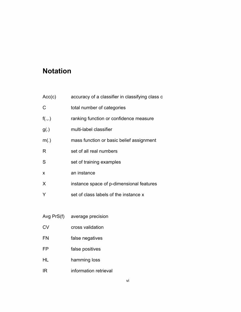
Notation
Acc(c) accuracy of a classifier in classifying class c
C total number of categories
f(.,.) ranking function or confidence measure
g(.) multi-label classifier
m(.) mass function or basic belief assignment
R set of all real numbers
S set of training examples
x an instance
X instance space of p-dimensional features
Y set of class labels of the instance x
Avg PrS(f) average precision
CV cross validation
FN false negatives
FP false positives
HL hamming loss
IR information retrieval
vii
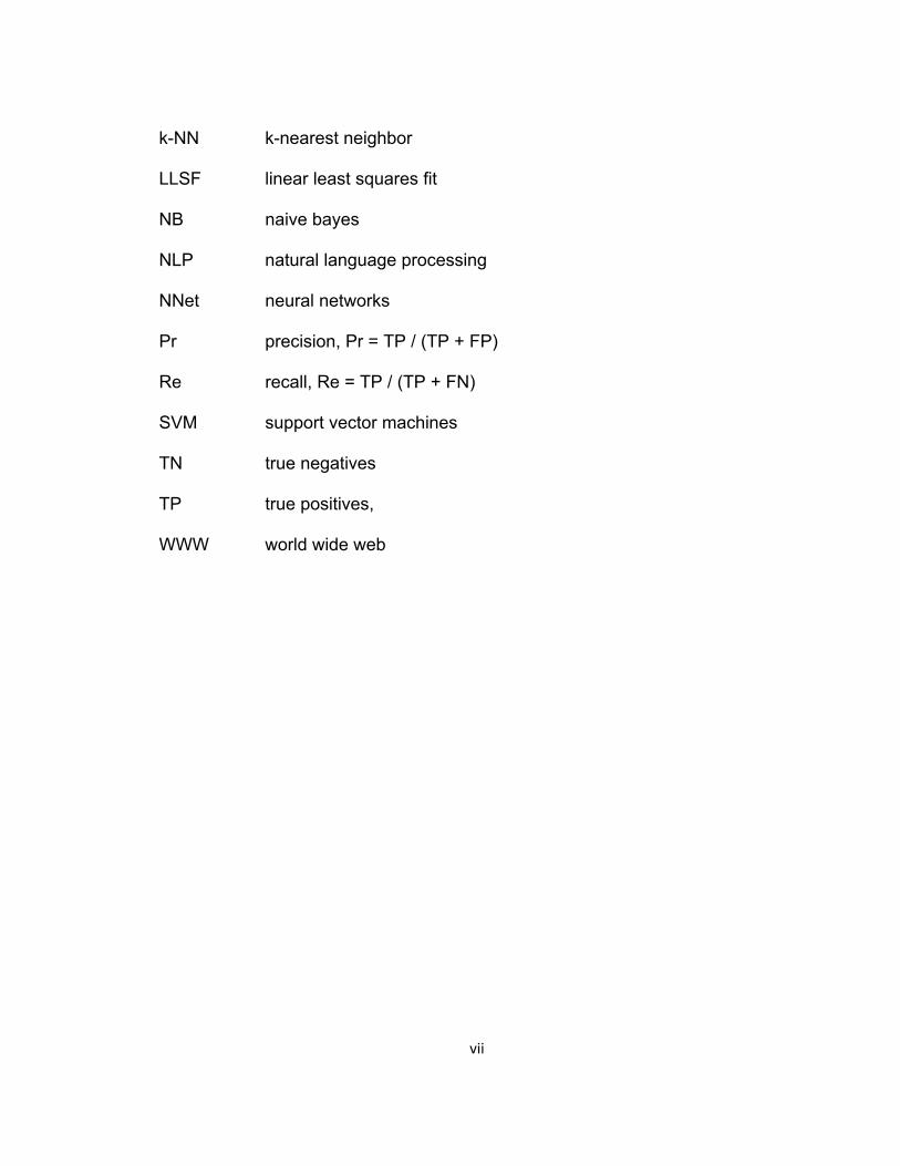
k-NN k-nearest neighbor
LLSF linear least squares fit
NB naive bayes
NLP natural language processing
NNet neural networks
Pr precision, Pr = TP / (TP + FP)
Re recall, Re = TP / (TP + FN)
SVM support vector machines
TN true negatives
TP true positives,
WWW world wide web
viii
List of Figures
Figure 5.1: Class distribution of 10,000 documents in experimental data, non-disjoint classes……………………………………………………………44
Figure 5.2: Number of documents in the experimental data having different number of class labels………………………………………………………...45
Figure 5.3: CPU times for different CV values and different number of features…………………………………………………………………………50
Figure 5.4: F-Macro values of different number of features for CV-1…....53
Figure 5.5: F-Macro values of different number of features for CV-2…....53
Figure 5.6: F-Macro values of different number of features for CV-3……54
Figure 5.7: F-Macro values of different number of features for CV-4……54
Figure 5.8: F-Macro values of different number of features for CV-5……55
Figure 5.9: F-Macro average values of different number of features…….55
Figure 5.10: F-Micro values of different number of features for CV-1……56
Figure 5.11: F-Micro values of different number of features for CV-2…...56
Figure 5.12: F-Micro values of different number of features for CV-3……57
Figure 5.13: F-Micro values of different number of features for CV-4……57
Figure 5.14: F-Micro values of different number of features for CV-5……58
Figure 5.15: F-Micro average values of different number of features……58
ix
List of Tables
Table 2.1: The macro-averaging and micro-averaging versions of the precision and recall performance criteria for domains with multi-label examples………………………………………………………………………..22
Table 4.1: Differences of different combining methods……………………33
Table 4.2: A generalized pattern table………………………………………35
Table 4.3: Subset 1 of the decision tree combination……………..………37
Table 4.4: Subset 2 of the decision tree combination………………..……37
Table 4.5: Subset 3 of the decision tree combination…………………..…38
Table 4.6: Subset 4 of the decision tree combination……………..………38
Table 4.7: Rule Generation of the decision tree combination…………….39
Table 5.1: Multi-label C4.5 results for different number of features……...47
Table 5.2: Average F-Macro and F-Micro values for 500 Features………48
Table 5.3: Average F-Macro and F-Micro values for 1000 Features…….48
Table 5.4: Average F-Macro and F-Micro values for 2000 Features…….49
Table 5.5: Total CPU time (min) for different CV’s of C4.5………………..49
Table 5.6: Cross-validation results for different algorithms………….……52
Table 5.7: F-Micro and F-Macro values for different number of
features…………………………………………………………………………59
CHAPTER 1 Introduction
In today’s world, most of the documents including publications, books,
messages, and articles are stored in the digital format and as a result, the
amount of electronic text information is increasing rapidly. The big increment in
online text information also increases the challenge of extracting relevant
knowledge. The need for tools that enhance people find, filter, and manage these
resources has grown. As a result, automatic organization of text document
collections has become a very important research area. A number of machine
learning techniques have been proposed to enhance automatic organization of
text data. There are two basic groups for these techniques which are the
supervised and unsupervised approaches. Supervised approach is the one
where pre-defined category labels are assigned to documents based on the
likelihood suggested by a training set of labeled documents; and the
unsupervised approach is the one where there is no need for human intervention
or labeled documents at any point in the whole process. Supervised approach is
used for document classification which we mostly deal with in this research, and
unsupervised approach is used for document clustering.
1

2
Machine learning is a subfield of artificial intelligence that is concerned
with the development of algorithms and techniques that make computers capable
of acquiring skill and integrating knowledge from data or experience, with the
objective of solving a given problem in a way analogical to human learning
(Michalski et al. 1998). Machine learning algorithms allow computers to learn by
automatically improving their performances based on their previous experiences.
Machine learning is related to data mining, statistics, and computer science since
it uses computational and statistical methods to extract information data
automatically.
Some of the machine learning applications is search engines, natural
language processing, syntactic pattern recognition, medical diagnosis,
bioinformatics, credit card fraud detection, stock market analysis, DNA sequence
classification, speech recognition, object recognition in computer vision including
face recognition, computer game programming and robot locomotion.
Classification is a particular task requiring machine learning and it has a
broad spectrum of applications including the entire machine learning applications
that we previously listed. Classification term generally describes the result of a
learning process by which a classification system is constructed. Classification
schemes or rules which are extracted from a training set data are known as
classifiers. The classification rules relate the class labels to some features and
this work considers as supervised learning in which pre-defined category labels

3
are assigned to documents based on the likelihood suggested by a training set of
labeled documents.
The traditional classification problem is to assign an object to one class.
However, in real world, it is very common to see that one example belongs to
several classes. This case is known as multi-label classification. In this research,
we are going to be working on the text document classification where multi-label
setting is the problem.
1.1 Document Classification
Text classification which is also known as text categorization is a
supervised learning task where pre-defined category labels are assigned to
documents based on the likelihood suggested by a training set of labeled
documents. The most popular approach was knowledge engineering before this
machine learning approach to text categorization. In knowledge engineering,
expert knowledge is used to define manually a set of rules on how to classify
documents under the pre-defined categories. Sebastiani (2002) discussed the
machine learning approach to text document classification leads to time and cost
savings in terms of expert manpower without failure in accuracy. We have a set
D of documents and a set S of pre-defined categories in the problem of text
classification The aim of text classification is to assign a Boolean value to each
<di,cj> pair, where di is an element of D and cj is an element of S. A true Boolean
value assigned to <di,cj> stands for the decision of assigning document di to
4
category cj, and the false Boolean value is assigned to <di,cj> stands for the
decision of not assigning document di to category cj. Our task in this problem is
to approximate the unknown target function f: DxS -> {true, false}. This function
describes the way the documents should actually be classified, by the classifier
function f': DxS -> {true, false} such that number of decisions of f and f' that do
not match is minimized.
There is a lot of learning algorithms which has been applied to text
document classification including k-nearest neighbor (k-NN), Support Vector
Machines (SVM), neural networks (NNet), linear least squares fit (LLSF), and
naive Bayes (NB). Yang and Liu (1999) presents a comparison of these learning
algorithms. All these techniques perform comparably when each category
contains over 300 documents. However; SVM, k-NN, and LLSF outperform
significantly NNet and NB when the number of positive training documents per
category is less than 10.
Document organization, text filtering and hierarchical categorization of
web pages are some of the interesting application areas of text categorization.
Document categorization is the task of structuring documents of a corporate
document base into folders. Text document categorization was used by Larkey
(1999) in order to organize patents into categories to enhance their search. The
process of classifying a dynamic collection of text documents into two disjoint
categories as relevant and irrelevant is known as text filtering. For example, an
email filter may be implemented to classify incoming messages as spam or not
5
spam, and block the spam messages. It is more effective and easier to navigate
in the hierarchy of categories first and restrict the search to the particular
categories of interest instead of posing a generic query to a general purpose
search engine. Koller and Sahami (1997) and by Dumais and Chen (2000)
mentioned the hierarchical classification of documents. The classification
problem is divided into smaller classification problems to classify documents
hierarchically.
1.2 Document Clustering
As we previously mentioned, document classification is a supervised
learning task whereas document clustering is an unsupervised learning task
which does not require pre-defined categories and labeled documents. After the
text clustering process, text documents are going to be grouped with higher intra-
group similarities and lower inter-group similarities. Information Retrieval (IR) is
one of the most important application areas of document clustering which has
been used to improve precision and recall. IR is also an efficient way of finding
similar documents. Koller and Sahami (1997) used document clustering in
automatic generation of hierarchical grouping of documents in document
browsing to organize the results returned by a search engine which was
designed by Zamir et al (1997).
6
Hierarchical clustering algorithms and partitioned clustering algorithms
(1999) are two main groups of machine learning algorithms for clustering.
Hierarchical algorithms produce nested partitions of data by splitting which is
known as divisive approach or merging which is the agglomerative approach
clusters based on the similarity among them. Divisive algorithms start with one
cluster of all data points and they split the most appropriate cluster until a
stopping criterion such as a requested number k of clusters is achieved at each
iteration. On the other hand, each item starts as an individual cluster in
agglomerative algorithms and the most similar pair of clusters is merged at each
step. Zhao and Karypis (2002) presented the evaluation of hierarchical clustering
algorithms for document data sets.
The data is grouped into un-nested non-overlapping partitions that locally
optimize a clustering criterion by partitioned clustering algorithms. K-means and
its variant bisecting k-means are the most popular partitioned clustering methods
which are applied to the text document domain. Steinbach et al (1999) showed
that the average-link algorithm generally performs better than single-link and
complete-link algorithms for the document data sets used in the experiments by
comparing agglomerative hierarchical techniques with k-means and bisecting k-
means.

7
1.3 Motivation
There are a lot of supervised machine learning techniques which have
been previously applied to text document classification. However in text
classification, there is a need of predefining the categories and assigning
category labels to the documents in the training set. Predefining the categories
and assigning category labels to the documents in the training set can be
extremely hard in large and dynamic text databases. We can give World Wide
Web (WWW) as an example of this kind of databases which will be hard to
defining the categories on.
Information retrieval is the science of searching, sorting, recovering, and
interpreting information in documents. Most of the documents including
publications, books, messages, and articles are stored in the digital format and
as a result, the amount of electronic text information is increasing rapidly. The big
increment in online text information also increases the challenge of extracting
relevant knowledge. The need for tools that enhance people find, filter, and
manage these resources has grown. As a result, automatic organization of text
document collections has become a very important research area in information
retrieval systems. The purpose of this kind of systems is to find and retrieve
categories of relevant documents in a collection of documents, and this can be
done by text document categorization.

8
Text document categorization process is time-consuming and the
computational cost of this process is extremely high. Text document
categorization is beyond human's ability due to the huge amount of documents
and that is why the need for solving multi-label classification problems are
increasing. We can say that solving the multi-label classification problems is the
only way to enable the people to manage resources and improve the accuracy
and efficiency of categorization.
1.4 Challenges and Research Objective
We can list the most common challenges of solving multi-label
classification problems as follow:
• For text categorization problems, input data space is extremely large.
These kinds of datasets consist of thousands of documents and they are
characterized by thousands of features. Training classifiers with
thousands of training examples has an extremely high computational cost
since the data take a while to run depending on the number of features.
• There are a lot of redundant features which are not informative and have
little discriminative power to predict category membership and they also
affect the computational cost and running time of the system. As a result,
it is desirable to run small subset of features instead of using too many

9
features since using too many features can give inaccurate classification
and it is the same thing with using insufficient number of features.
• Curse of dimensionality is another problem that we deal with in this
project. This problem occurs when the dimension of the feature space is
much higher than the number of the training examples and it makes
performing the numerical computations harder.
• Most documents have fewer words comparing to the total number of
words in the document collection. As a result, text documents are
represented as sparse vectors when we use the words as features which
make the learning process harder.
• In our data, it is common to see some examples have few examples and
some other has a lot of examples which means the multi-label examples
are imbalanced. Imbalanced training data can affect classification
accuracy as we can see in the previous studies (Liu and Motoda 2002).
• As we mentioned previously, we preferred to use small subset of features
instead of using too many features at the same time since it makes the
computational costs extremely high. One important problem that we deal
with in this project is to generate small subset of features since we
sometimes had noisy examples at the end of this process. Noisy
information in the training examples may affect the results and it is an
important problem to deal with.

10
When we check the computational costs of the multi-label classification
problems, we can easily see that it is necessary to find alternative learning
mechanism to reduce these costs and give accurate results at the same time.
Our objective in this research project is to run different algorithms on the same
data, compare the results of these algorithms for computational cost and
accuracy and implement a new possible alternative mechanism to have less cost
and more accuracy as much as possible at the same time.
1.5 Thesis Organization
Chapter 2 starts with the definition of multi-label classification and
continues with the classification methods. In this project, we only deal with the
algorithm based classification methods. In Chapter 2, we also described our
performance criteria to compare the performances of different multi-label
classification algorithms.
We are describing the multi-label classification algorithms that we used in
this research in Chapter 3. We mostly used multi-label C4.5 in this project and
we compared the performance of this algorithm with the other existing algorithms
including Boostexter.
In Chapter 4, we proposed a method for combining the decision trees
which was described by Kim (2001). We mentioned the steps to implement the
algorithm for decision tree combination and we talked about the way that we do

11
the rule generation to fix the misclassification to attain better results on
combining.
In Chapter 5, we provided the experiment results of different algorithms
including multi-label C4.5 and Boostexter. We compared the performances of
different algorithms by the criteria that we described at Chapter 2. We also
provided the decision tree combination results that we described at Chapter 4.
CHAPTER 2 Multi-label Classification
Multi-label classification deals with the value of |L| > 2 where L is the set of
disjoint labels whereas traditional single-label classification deals with learning
from a set of examples that are associated with a single label l from the same set
of disjoint labels as in the multi-label classification L, |L| > 1. Learning problem is
called a binary classification problem when the value of |L| = 2 and the problem
called multi-label classification problem when |L| > 2. As a result, we can say that
the traditional classification problem is to assign an object to one class whereas
one example belongs to several classes in multi-label classification problem.
The set of examples are associated with a set of labels in multi-label
classification problem. Multi-label classification was previously used on search
engines, natural language processing, syntactic pattern recognition, medical
diagnosis, bioinformatics, credit card fraud detection, stock market analysis, DNA
sequence classification, speech recognition, object recognition in computer vision
including face recognition, computer game programming and robot locomotion.
12
13
i
2.1 Classification Methods
There are two basic categories of existing multi-label classification
methods which are the problem transformation methods, and the algorithm
adaptation methods. Problem transformation methods are the ones which
transform the multi-label classification problem into one or more traditional single-
label classification problems. Algorithm adaptation methods for multi-label
classification are the methods which extend specific learning algorithms in order
to directly deal with multi-label data.
2.1.1. Algorithm Adaptation Methods
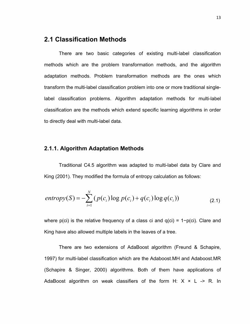
Traditional C4.5 algorithm was adapted to multi-label data by Clare and
King (2001). They modified the formula of entropy calculation as follows:
1( ) ( ( ) log ( ) ( ) log ( ))
N
i i ii
entropy S p c p c q c q c=
= − +∑ (2.1)
where p(ci) is the relative frequency of a class ci and q(ci) = 1−p(ci). Clare and
King have also allowed multiple labels in the leaves of a tree.
There are two extensions of AdaBoost algorithm (Freund & Schapire,
1997) for multi-label classification which are the Adaboost.MH and Adaboost.MR
(Schapire & Singer, 2000) algorithms. Both of them have applications of
AdaBoost algorithm on weak classifiers of the form H: X × L -> R. In
14
AdaBoost.MH algorithm, an example can be labeled with l if the output sign of
the weak classifiers is positive for a new example x and a label l. We do not
label an example with l if the same value is negative. In AdaBoost.MR algorithm,
the output of the weak classifiers is considered for ranking each of the labels in L
where L is the set of disjoint labels.
AdaBoost.MH AdaBoost.MR algorithms are adaptations of a specific
learning approach. However, these algorithms use a problem transformation.
Every example of (x, Y) is decomposed into |L| examples (x, l, Y[l]), for all l L,
where Y[l] = 1 if l Y, and otherwise [l] = −1.
ML-kNN (Zhang & Zhou, 2005) is an improvement of the traditional kNN
learning algorithm for multi-label data. kNN algorithm was used by the improved
ML-kNN algorithm independently for each label l. The new improved ML-kNN
algorithm finds the k nearest examples to the test instance and considers the k
nearest examples as labeled at least with l as positive and the rest as negative.
ML-kNN algorithm is also capable of producing a ranking of the labels as an
output.
Two more systems for multi-label document classification were presented
by Luo and Zincir-Heywood (2005) and these algorithms were based on the kNN
classifier too. The main involvement of their research was on the pre-processing
stage in order to represent the documents effectively. The system that Luo and
Zincir-Heywood described finds the k nearest examples initially in order to
15
classify the new instance. The next step of this system is to increase a
corresponding counter for each label in which the examples appear. The last
step of the system is to output N labels with the largest counts. They choose the
N value based on the number of labels of the instance. Since the number of
labels of a new instance is unknown, this is an unacceptable strategy for real-
world use.
A probabilistic generative model was proposed by McCallum (1999) and in
this model, each label generated different words. The system produced a multi-
label document by a mixture of the word distributions of its labels based on this
model described by McCallum. In this model, expectation maximization method
was used to calculate which labels were both the mixture weights and the word
distributions for each label where the parameters of the model described by
McCallum were learned from labeled training documents by maximum posteriori
estimation method. In this model, each different set of labels was considered as
a new class by themselves.
A ranking algorithm for multi-label classification was proposed by Elisseeff
and Weston (2002). They used the SVMs (Support Vector Machines) method on
their algorithm. SVMs are a set of supervised learning methods that are used for
classification and these methods belong to linear classifiers. The aim of these
methods is to minimize a cost function while maintaining a large margin. Ranking
loss was the cost function that Elisseeff and Weston used for their algorithm and
this function was defined as the average fraction of incorrectly ordered labels. As
16
we previously mentioned, ranking algorithm has the disadvantage since it does
not output a set of labels.
Two improvements for SVMs were presented by Godbole and Sarawagi
(2004) for multi-label classification. The first improvement for SVMs was to be
used with any classification algorithm. The idea behind this algorithm was to
extend the original data set with |L| extra features containing the predictions of
each binary classifier. In the following step, extended datasets were used in
order to train |L| new binary classifiers. The binary classifiers of the first step
were initially used and their output was added to the features of the example to
form a meta-example for classification. At the second step, binary classifiers
classify the meta-example. The new approach described by Godbole and
Sarawagi takes into consideration the potential dependencies among the
different labels through this extension.
The second improvement which was presented by Godbole and Sarawagi
(2004) was SVM-specific and this method concerned the margin of SVMs in
multi-label classification problems. Godbole and Sarawagi used two different
approaches to improve the margin. The first approach to improve the margin was
to remove very similar negative training instances which are within a threshold
distance from the learnt hyper plane, and the second approach that they used
was to remove negative training instances of a complete class when it is very
similar to the positive class. They implemented their method based on a
confusion matrix which is estimated by using any fast and moderately accurate

17
classifier on a held out validation set. We can say that the second approach for
margin improvement is not dependent to SVMs.
Thabtah, Cowling & Peng (2004) described and algorithm called MMAC
which follows the associative classification pattern. The associative classification
pattern uses association rule mining to deal with the construction of classification
rule sets. The aim of MMAC algorithm is to learn an initial set of classification
rules by using association rule mining, and to remove the examples which are
associated with th rule set. This algorithm learns a new rule set from the
remaining examples until no further frequent items are left. The MMAC algorithm
ranks the labels depending on the corresponding individual rule support.
2.2 Problem Statement
We cannot say that all datasets are equally multi-label. The number of
labels on each example is small comparing to |L| in some datasets, whereas the
number of labels on each example is large comparing to |L| in some other
datasets. The number of labels on each example can be a parameter that affects
the performance of the different multi-label methods.
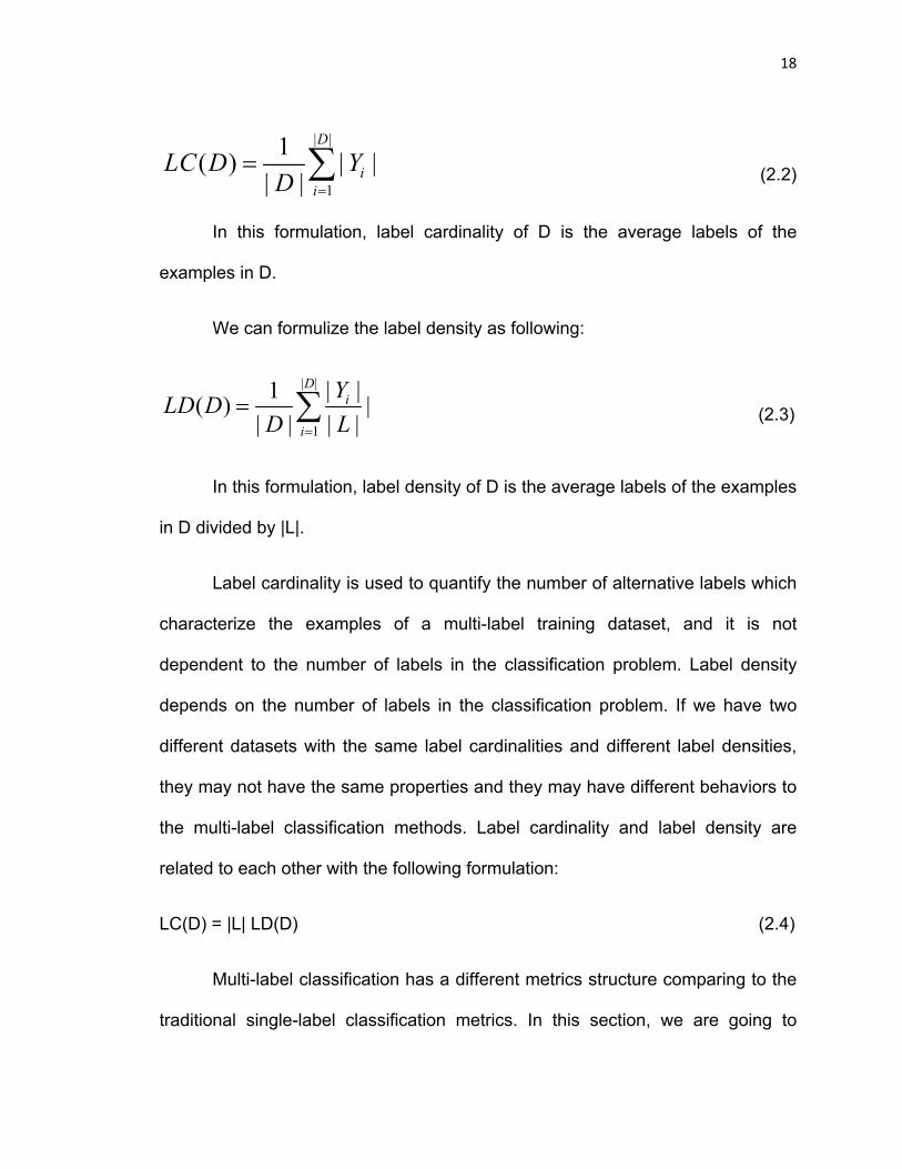
In this section, we are going to introduce the label cardinality and label
density concepts of a dataset where D is the multi-label data set consisting of |D|
multi-label examples (xi, Yi), i = 1..|D|.
We can formulize the label cardinality as following:
18
| |
1
1( ) | || |
D
ii
LC D YD =
= ∑ (2.2)
In this formulation, label cardinality of D is the average labels of the
examples in D.
We can formulize the label density as following:
| |
1
| |1( ) || | | |
Di
i
YLD DD L=
= ∑ (2.3)
In this formulation, label density of D is the average labels of the examples
in D divided by |L|.
Label cardinality is used to quantify the number of alternative labels which
characterize the examples of a multi-label training dataset, and it is not
dependent to the number of labels in the classification problem. Label density
depends on the number of labels in the classification problem. If we have two
different datasets with the same label cardinalities and different label densities,
they may not have the same properties and they may have different behaviors to
the multi-label classification methods. Label cardinality and label density are
related to each other with the following formulation:
LC(D) = |L| LD(D) (2.4)
Multi-label classification has a different metrics structure comparing to the
traditional single-label classification metrics. In this section, we are going to
19
present the metrics of multi-label classification. We define D as a multi-label
evaluation dataset, consisting of |D| multi-label examples (xi, Yi), i = 1..|D|, Yi
L. We define H as a multi-label classifier and Zi = H(xi) is the set of labels
predicted by H for example xi.
Hamming Loss was defined by Schapire and Singer (2000) as the
following:
| |
1
| |1( , )| | | |
Di i
i
Y ZHL H DD L=
Δ= ∑ (2.5)
In this formulation, Δ is the symmetric difference of two datasets and defined as
the XOR operation in Boolean logic.
Godbole & Sarawagi (2004) used the following metrics of accuracy,
precision, and recall for the evaluation of H on D where H is the multi-label
classifier and D is the multi-label evaluation dataset:
| |
1
| |1( , )| | |
Di i
i i i
Y ZAccuracy H D|D Y Z=
∩=
∪∑ (2.6)
| |
1
| |1( , )| | | |
Di i
i i
Y ZPrecision H DD Z=
∩= ∑ (2.7)
| |
1
| |1( , )| | | |
Di i
i i
Y ZRecall H DD Y=
∩= ∑ (2.8)
20
Boutell et al. (2004) used an alpha parameter to provide a more
generalized version of the accuracy formulation where α ≥ 0, and called the alpha
parameter as forgiveness rate:
| |
1
| |1( , ) ( )| | | |
Di i
i i i
Y ZAccuracy H DD Y Z=
∩=
∪∑ α (2.9)
The aim of this parameter is to control the forgiveness of errors that are
made in label prediction.
2.3 Performance Criteria
Let X be a p-dimensional instance space and Y a set of classes, and let
each example, xi X, belong to a subset Yi Y. Given a set of training
examples,
S = {(x1; Y1),…,(xn,Yn)}, we want to induce a classifier, g : X -> 2y, with
maximum classification performance. Let us first summarize the performance
criteria used by the field of information retrieval for single-label domains, denoting
by TP (true positives) the number of correctly classified positive examples, by FN
(false negatives) the number of positive examples misclassified as negative, by
FP (false positives) the number of negative examples misclassified as positive
ones, and by TN (true negatives) the number of correctly classified negative
examples. These four quantities define precision and recall as follows:
21
TPPrTP FP
=+ (2.10)
TPReTP FN
=+ (2.11)
Observing that the user often wants to maximize both of them, while
balancing their values, van Rijsbergen (1979) combined precision and recall in a
single formula, Fβ, that is parameterized by the user-specified β [0,∞) that
quantifies the relative importance ascribed to either criterion:
2
2
1)xPrxReFxPr Reβ
(β +=
β + (2.12)
Here, β > 1 gives more weight to recall and β < 1 gives more weight to
precision; Fβ converges to recall if β -> ∞ and to precision if β = 0. The situation
where precision and recall are deemed equally relevant is marked by β = 1, in
which case F1 degenerates to the following equation:
12xPrxReFPr Re
=+ (2.13)
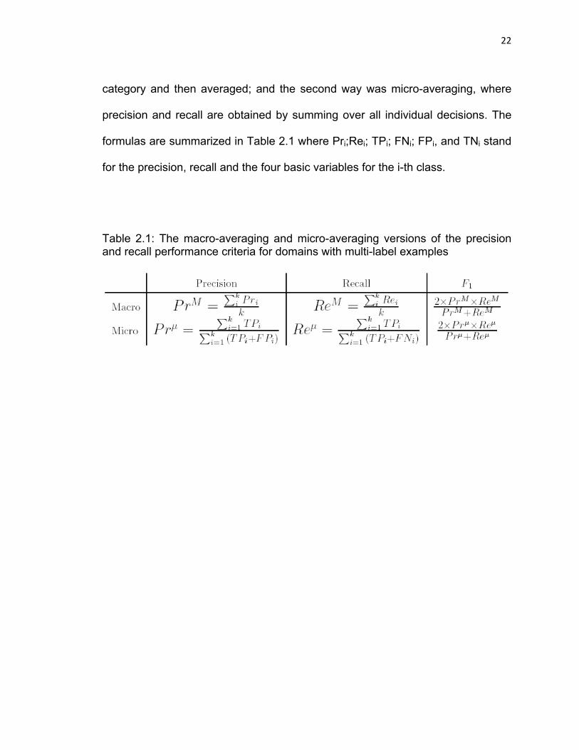
Based on these preliminaries, Yang (1999) proposed two alternative ways
these criteria can be generalized for domains with multi-label examples. The fist
way was macro-averaging, where precision and recall are first computed for each
22
category and then averaged; and the second way was micro-averaging, where
precision and recall are obtained by summing over all individual decisions. The
formulas are summarized in Table 2.1 where Pri;Rei; TPi; FNi; FPi, and TNi stand
for the precision, recall and the four basic variables for the i-th class.
Table 2.1: The macro-averaging and micro-averaging versions of the precision and recall performance criteria for domains with multi-label examples

CHAPTER 3 Multi-label Classification Algorithms
In this chapter, we are going to discuss different algorithms to apply to
multi-label classification or text document categorization. Two basic approaches
of multi-label classification problems are problem transformation and algorithm
adaptation as we mentioned on the previous section. There are various learning
algorithms and in this section, we are going to discuss the specific methods that
we used in our experiments for multi-label classification. AdaBoost.MH and
ADTree algorithms are multi-label learning algorithms, and C4.5 and k-nearest
neighbor algorithms are single-label learning algorithms.
3.1 Boosting Algorithms
Boosting is a machine learning algorithm based on Kearns' (1988) idea.
He was seeking the answer of the question: can a set of weak learners create a
single strong learner? As we can understand from this question, the idea behind
the boosting algorithms is to use the wrongly classified examples more often so
that the classifier can learn and correctly classify the wrongly classified
examples.
23
24
The first boosting algorithms were used by Robert Schapire (1990) which
was the recursive majority gate formulation and by Yoav Freund which was the
boost by majority. The first boosting algorithms that we mentioned were not
adaptive which means they were not able to implement the weak learners idea
with a full capacity.
There is a lot of boosting algorithms but most of them were not able to
adapt to the weak learners idea. The first boosting algorithm was presented by
Schapire (1990) and more efficient variations followed, including Adaptive
Boosting, AdaBoost (Freund and Schapire 1996; Freund and Schapire 1997)
which is the most populer boosting algorithm and AdaBoost is the first algorithm
which was able to adapt to the weak learners idea. Schapire and Singer (1999)
then introduced two extensions to their boosting algorithms which are
AdaBoost.MH and AdaBoost.MR. The former induces a classifier that minimizes
the Hamming distance between the example's correct class labels and those
proposed by the classifier; the latter provides label ranking, seeking to output
higher rankings for correct class labels. This lays the foundations for BoosTexter
which includes four earlier versions of AdaBoost.MH and AdaBoost.MR
algorithms.
3.1.1 AdaBoost.MH algorithm
AdaBoost is a machine learning meta-algorithm and it can be used with
other learning algorithms to improve the performance. AdaBoost is the first
25
boosting algorithm which adapts to the weal classifier idea. This algorithm calls a
weak classifier simultaneously and for each of them, the algorithm updates a
distribution of weights which is a measure of importance of the examples in the
dataset. The idea behind the AdaBoost algorithm is to use the wrongly classified
examples more often so that the classifier can learn and correctly classify the
wrongly classified examples. So we can say that for each round, AdaBoost
algorithm increases the weights of misclassified examples so that it focus on
those misclassified examples to learn based on its previous experience to
correctly classify those examples.
We can give the steps of AdaBoost algorithm as the following:
Given: (x1,Y1),...,(xn; Y n ) where xi X, Yi Y
Initialize D1(i,c) = 1/(nC), where C is the size of Y.
Do for t = 1,...,T, where T is the number of boosting iterations:
• Pass distribution Dt to weak learner.
• Get weak hypothesis ht: X x Y -> R.
• Choose αt R
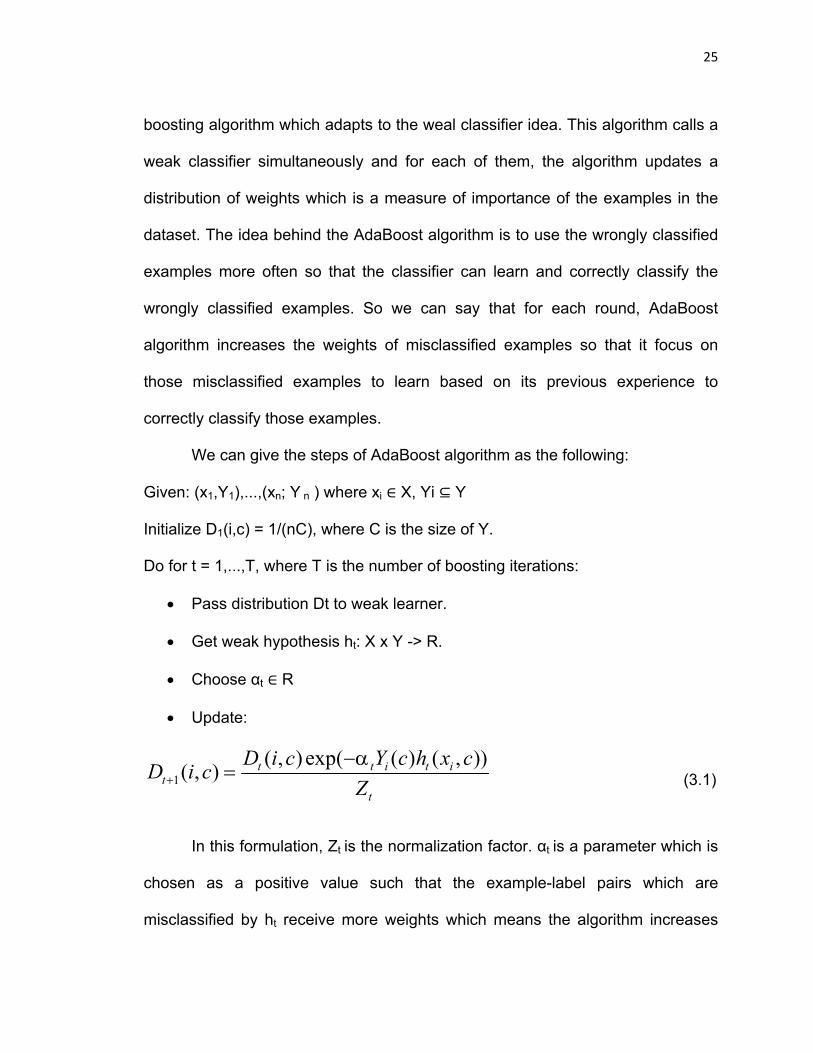
• Update:
1( , ) exp( ( ) ( , ))( , ) t t i t
tt
D i c Y c h x cD i cZ+
i−α= (3.1)
In this formulation, Zt is the normalization factor. αt is a parameter which is
chosen as a positive value such that the example-label pairs which are
misclassified by ht receive more weights which means the algorithm increases
26
1
( , ) ( , )T
t tt
the weights of misclassified examples so that it focus on those misclassified
examples to learn based on its previous experience to correctly classify those
examples.
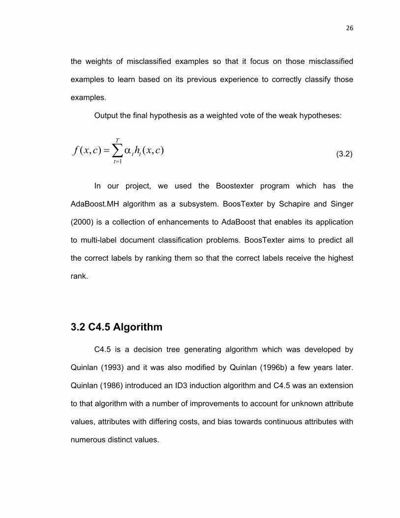
Output the final hypothesis as a weighted vote of the weak hypotheses:
x c h x c=
= α∑f (3.2)
In our project, we used the Boostexter program which has the
AdaBoost.MH algorithm as a subsystem. BoosTexter by Schapire and Singer
(2000) is a collection of enhancements to AdaBoost that enables its application
to multi-label document classification problems. BoosTexter aims to predict all
the correct labels by ranking them so that the correct labels receive the highest
rank.
3.2 C4.5 Algorithm
C4.5 is a decision tree generating algorithm which was developed by
Quinlan (1993) and it was also modified by Quinlan (1996b) a few years later.
Quinlan (1986) introduced an ID3 induction algorithm and C4.5 was an extension
to that algorithm with a number of improvements to account for unknown attribute
values, attributes with differing costs, and bias towards continuous attributes with
numerous distinct values.
27
C4.5 uses the information entropy concept to measure the information of a
node and this algorithm builds decision trees from training data by using this
concept. This algorithm examines the information gain, which is the effective
decrease in entropy that results from choosing a feature to split the data at a
particular node in the tree. The feature which has the highest information gain is
the best for discriminating among cases at that node, and as a result, it will be
the one which makes the decision.
Quinlan (1996b) showed that the new version of C4.5 has higher
predictive accuracies for smaller decision trees. Williams et al. (2006) compared
four different machine learning algorithms which are the Bayesian network, naive
Bayes, naive Bayes tree, and C4.5 decision tree, and they attained the best
results for real-time classification with C4.5 algorithm in their IP traffic flow
classification study. In that study, all algorithms had similar classification
accuracies, but the C4.5 algorithm was significantly faster than the other
algorithm when they compare the classification speed. Based on previous
experiences and experiments, we can say that the C4.5 algorithm is a good
choice for practical classification due to the ease of its interpretability and its
ability to deal with numeric attributes, missing values, and noisy data.
The standard machine learning algorithm C4.5 was extended to allow
multi-label classes by Clare, A. (2003). In the multi-label version of C4.5, each
class was taken in turn and made binary C4.5 classifiers. For example, a
classifier that could predict either class “1/0/0/0” or “not 1/0/0/0”.

28
C4.5 algorithm is efficient and robust. This algorithm produces a decision
tree, or a set of symbolic rules as an output. In C4.5 algorithm, the tree is
constructed top down. The attribute is chosen which best classifies the remaining
training examples for each node.

CHAPTER 4 Decision Tree Combination
The last step of our project was to combine the decision trees. We used
the method described by Kim (2001) to combine the decision trees. The most
common combining methods are Bagging method, M-method, and Stacking
method. Kim (2001) introduced a new method in his paper which uses cross-
validation or bootstrap as a re-sampling technique and discretization as a
combining method and achieved better prediction accuracy than a single
decision tree algorithm. Also, this method performs reasonably well with fewer
numbers of re-samples compared to the Bagging and Boosting methods.
y = (y1; … ; yN)T is the class variable observed on N instances and the
observed data matrix is X = (x1; … ; xN)T , where xi = (x1; … ; xp)i denote the
observed vector for ith instance. X is a p-dimensional measurement space
containing all possible values of x1; … ; xp. Xs is the disjoint partitions of X such
that X = Us Xs. A decision tree learning algorithm partitions the data space into
sub-regions and the algorithm finds Xs by this way which means the distribution
of classes is going to be more homogeneous. It provides a tree-structure
according to the split taking the {Is xi ≤ c?} form for ordered variables or of {Is xj
29
30
C?} for nominal variables. In these forms, c is an arbitrary point in the range of xi
and C is in the range of all subsets of categories on xj. At this point, we can grow
a sequence of trees by recursively choosing splits which is going to maximize the
homogeneity of the classes of the node. Tree growing will be going on until the
stopping criteria are satisfied. After that point, a decision tree is going to be
selected by pruning back the tree based on certain criteria. The distribution of
classes in each terminal node determines the predictions.
Because of the fact that the decision tree algorithms such as C4.5
(Quinlan, 1993) or CART (Breiman, Friedman, Olshen and Stone, 1984) provide
intuitive interpretations, they have attracted many researchers. In Computer
Science and Statistics areas, combining methods become very important since
there is a need to increase the prediction accuracy of decision trees. Many
researchers have used the combining predictions technique of individually
trained classifiers when they classify the future instances. After Wolpert (1992)
described the stacking algorithm in the context of regression, the idea of
combining predictions of different models become much more popular. Stacked
regression algorithm was developed by Breiman (1996b) by adopting backward
elimination and ridge regression. Methods such as Bagging (Breiman, 1996a)
and Boosting (Freund and Schapire, 1996) was very successful in the sense of
improving the accuracy of the classification algorithm in the context of
classification which we can see at the experiments of Bauer and Kohavi (1999),
Opitz (1999), and Dietterich (2000) for comparison results. These methods
31
depend on re-sampling techniques in order to obtain different learning samples
for each of the decision trees. There are many combining methods which were
previously developed. We can give Schapire and Singer (1999), Breiman (2000),
and Web (2000) as an example of some of the most important combining
methods.
4.1 Methodology
The first step of decision tree combination methods in classification is to
generate many different learning samples via re-sampling technique. Let L be the
training data and b re-samples denoted by L1; … ;Lb are generated from L. Then
we can apply the classification algorithm and construct classifiers on these
samples. If an algorithm A is used, b classifiers denoted by T1; … ; Tb are
constructed based on L1; … ;Lb, respectively. T1; … ; Tb are constructed by the
same algorithm.
There are three basic components of combining methods where the first
component is the selection of re-sampling technique, the second component is
the number of participating classification algorithms, and the third one is
combining method to get overall prediction. Bagging uses bootstrap technique for
the first and majority voting for the third. It uses only one classification algorithm
for the second component because its main purpose is to increase the accuracy
of the specific classification algorithm.
32
A method to combine several classification algorithms without re-sampling
technique was described by Mojirsheibani (1999). The main aim of this method
was to combine different algorithms instead of combining prediction results of
one algorithm. Several classification algorithms A1; … ; Ab are used to generate
classifiers T1; … ; Tb, respectively as an illustration. The prediction results based
on T1; … ; Tb are used to predict the learning or evaluation data. This method
does not re-sample the learning dataset L. This method uses discretization to
combine the predictions. This method is not appropriate for combining
predictions of the specific algorithm since it requires several classification
algorithms to be applied on the same learning sample. Mojirsheibani’s algorithm
does not have the first component while several classification algorithms are
required for the second. Discretizations of the predictions are utilized as the third
component to get overall prediction of each instance. This method is called the
M-method.
Wolpert (1992) and Breiman (1996b) used the leave-one-out data which
they called level-one data for the stacking algorithm. The stacking algorithm uses
leave-one-out technique for the first component. It also requires several
regression methods for the second as in M-method, then combining predictions
is achieved by ridge regression based on the prediction results of all participating
regression methods. Stacking method is designed for the regression problem.
The differences of the existing and the new combining methods are shown
in Table 4.1. As we can see in this table, the new method that we used on our
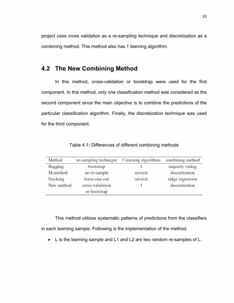
33
project uses cross validation as a re-sampling technique and discretization as a
combining method. This method also has 1 learning algorithm.
4.2 The New Combining Method
In this method, cross-validation or bootstrap were used for the first
component. In this method, only one classification method was considered as the
second component since the main objective is to combine the predictions of the
particular classification algorithm. Finally, the discretization technique was used
for the third component.
Table 4.1: Differences of different combining methods
This method utilizes systematic patterns of predictions from the classifiers
in each learning sample. Following is the implementation of the method:
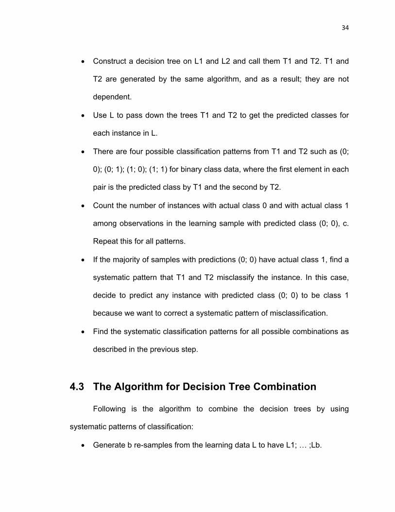
• L is the learning sample and L1 and L2 are two random re-samples of L.
34
• Construct a decision tree on L1 and L2 and call them T1 and T2. T1 and
T2 are generated by the same algorithm, and as a result; they are not
dependent.
• Use L to pass down the trees T1 and T2 to get the predicted classes for
each instance in L.
• There are four possible classification patterns from T1 and T2 such as (0;
0); (0; 1); (1; 0); (1; 1) for binary class data, where the first element in each
pair is the predicted class by T1 and the second by T2.
• Count the number of instances with actual class 0 and with actual class 1
among observations in the learning sample with predicted class (0; 0), c.
Repeat this for all patterns.
• If the majority of samples with predictions (0; 0) have actual class 1, find a
systematic pattern that T1 and T2 misclassify the instance. In this case,
decide to predict any instance with predicted class (0; 0) to be class 1
because we want to correct a systematic pattern of misclassification.
• Find the systematic classification patterns for all possible combinations as
described in the previous step.
4.3 The Algorithm for Decision Tree Combination
Following is the algorithm to combine the decision trees by using
systematic patterns of classification:
• Generate b re-samples from the learning data L to have L1; … ;Lb.
35
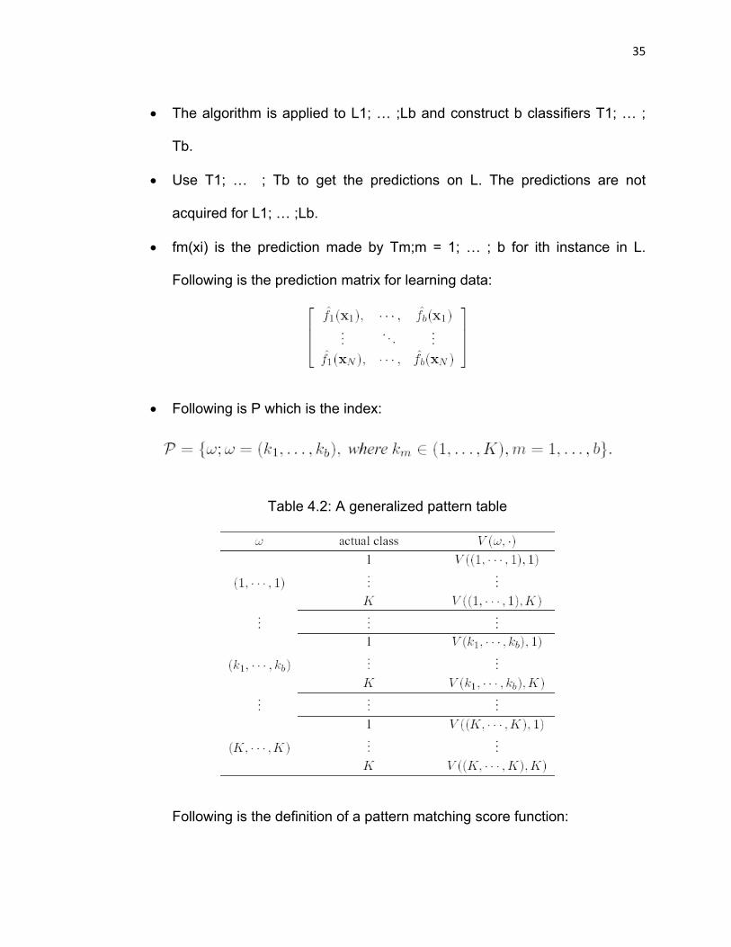
• The algorithm is applied to L1; … ;Lb and construct b classifiers T1; … ;
Tb.
• Use T1; … ; Tb to get the predictions on L. The predictions are not
acquired for L1; … ;Lb.
• fm(xi) is the prediction made by Tm;m = 1; … ; b for ith instance in L.
Following is the prediction matrix for learning data:
• Following is P which is the index:
Table 4.2: A generalized pattern table
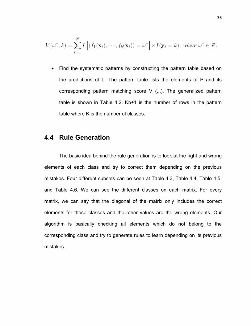
Following is the definition of a pattern matching score function:
36
• Find the systematic patterns by constructing the pattern table based on
the predictions of L. The pattern table lists the elements of P and its
corresponding pattern matching score V (.,.). The generalized pattern
table is shown in Table 4.2. Kb+1 is the number of rows in the pattern
table where K is the number of classes.
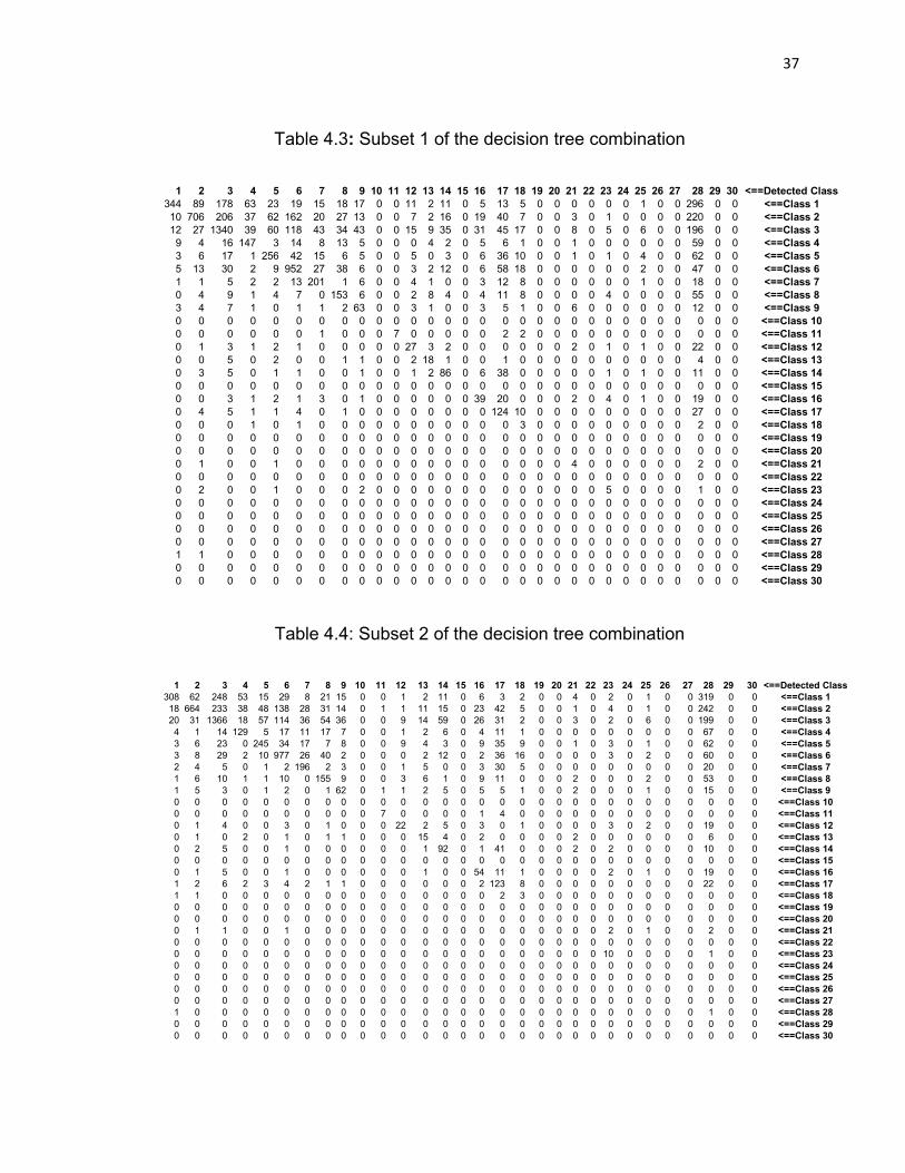
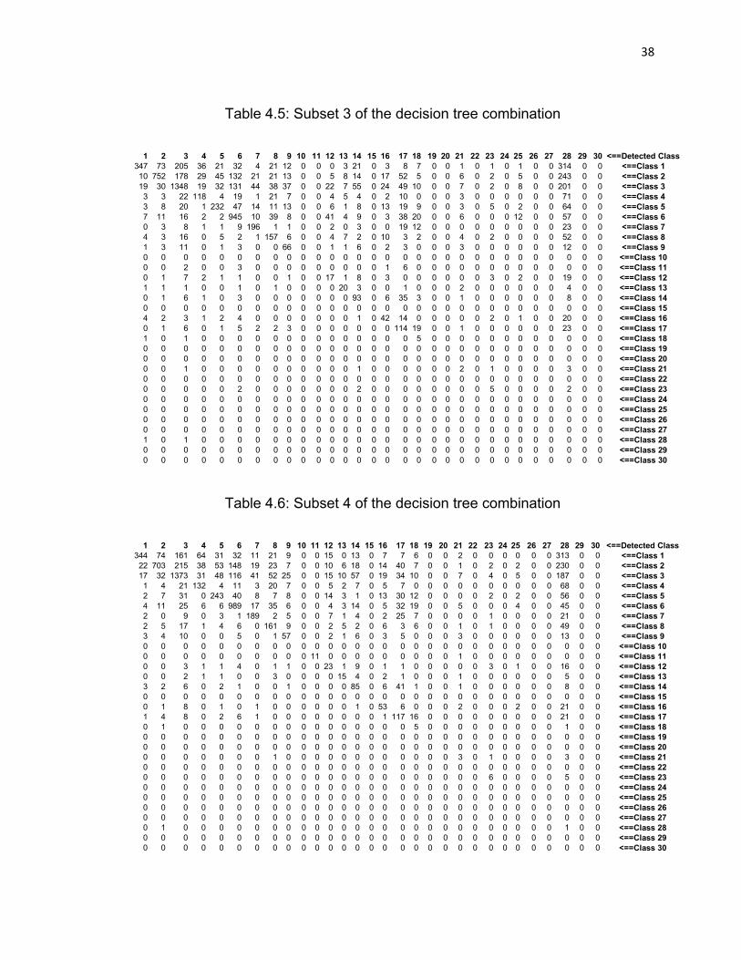
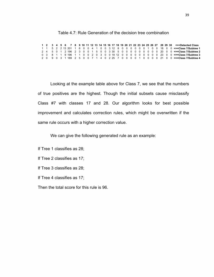
4.4 Rule Generation
The basic idea behind the rule generation is to look at the right and wrong
elements of each class and try to correct them depending on the previous
mistakes. Four different subsets can be seen at Table 4.3, Table 4.4, Table 4.5,
and Table 4.6. We can see the different classes on each matrix. For every
matrix, we can say that the diagonal of the matrix only includes the correct
elements for those classes and the other values are the wrong elements. Our
algorithm is basically checking all elements which do not belong to the
corresponding class and try to generate rules to learn depending on its previous
mistakes.
37
Table 4.3: Subset 1 of the decision tree combination
1 2 3 4 5 6 7 8 9 10 11 12 13 14 15 16 17 18 19 20 21 22 23 24 25 26 27 28 29 30 <==Detected Class344 89 178 63 23 19 15 18 17 0 0 11 2 11 0 5 13 5 0 0 0 0 0 0 1 0 0 296 0 0 <==Class 110 706 206 37 62 162 20 27 13 0 0 7 2 16 0 19 40 7 0 0 3 0 1 0 0 0 0 220 0 0 <==Class 212 27 1340 39 60 118 43 34 43 0 0 15 9 35 0 31 45 17 0 0 8 0 5 0 6 0 0 196 0 0 <==Class 39 4 16 147 3 14 8 13 5 0 0 0 4 2 0 5 6 1 0 0 1 0 0 0 0 0 0 59 0 0 <==Class 43 6 17 1 256 42 15 6 5 0 0 5 0 3 0 6 36 10 0 0 1 0 1 0 4 0 0 62 0 0 <==Class 55 13 30 2 9 952 27 38 6 0 0 3 2 12 0 6 58 18 0 0 0 0 0 0 2 0 0 47 0 0 <==Class 61 1 5 2 2 13 201 1 6 0 0 4 1 0 0 3 12 8 0 0 0 0 0 0 1 0 0 18 0 0 <==Class 70 4 9 1 4 7 0 153 6 0 0 2 8 4 0 4 11 8 0 0 0 0 4 0 0 0 0 55 0 0 <==Class 83 4 7 1 0 1 1 2 63 0 0 3 1 0 0 3 5 1 0 0 6 0 0 0 0 0 0 12 0 0 <==Class 90 0 0 0 0 0 0 0 0 0 0 0 0 0 0 0 0 0 0 0 0 0 0 0 0 0 0 0 0 0 <==Class 100 0 0 0 0 0 1 0 0 0 7 0 0 0 0 0 2 2 0 0 0 0 0 0 0 0 0 0 0 0 <==Class 110 1 3 1 2 1 0 0 0 0 0 27 3 2 0 0 0 0 0 0 2 0 1 0 1 0 0 22 0 0 <==Class 120 0 5 0 2 0 0 1 1 0 0 2 18 1 0 0 1 0 0 0 0 0 0 0 0 0 0 4 0 0 <==Class 130 3 5 0 1 1 0 0 1 0 0 1 2 86 0 6 38 0 0 0 0 0 1 0 1 0 0 11 0 0 <==Class 140 0 0 0 0 0 0 0 0 0 0 0 0 0 0 0 0 0 0 0 0 0 0 0 0 0 0 0 0 0 <==Class 150 0 3 1 2 1 3 0 1 0 0 0 0 0 0 39 20 0 0 0 2 0 4 0 1 0 0 19 0 0 <==Class 160 4 5 1 1 4 0 1 0 0 0 0 0 0 0 0 124 10 0 0 0 0 0 0 0 0 0 27 0 0 <==Class 170 0 0 1 0 1 0 0 0 0 0 0 0 0 0 0 0 3 0 0 0 0 0 0 0 0 0 2 0 0 <==Class 180 0 0 0 0 0 0 0 0 0 0 0 0 0 0 0 0 0 0 0 0 0 0 0 0 0 0 0 0 0 <==Class 190 0 0 0 0 0 0 0 0 0 0 0 0 0 0 0 0 0 0 0 0 0 0 0 0 0 0 0 0 0 <==Class 200 1 0 0 1 0 0 0 0 0 0 0 0 0 0 0 0 0 0 0 4 0 0 0 0 0 0 2 0 0 <==Class 210 0 0 0 0 0 0 0 0 0 0 0 0 0 0 0 0 0 0 0 0 0 0 0 0 0 0 0 0 0 <==Class 220 2 0 0 1 0 0 0 2 0 0 0 0 0 0 0 0 0 0 0 0 0 5 0 0 0 0 1 0 0 <==Class 230 0 0 0 0 0 0 0 0 0 0 0 0 0 0 0 0 0 0 0 0 0 0 0 0 0 0 0 0 0 <==Class 240 0 0 0 0 0 0 0 0 0 0 0 0 0 0 0 0 0 0 0 0 0 0 0 0 0 0 0 0 0 <==Class 250 0 0 0 0 0 0 0 0 0 0 0 0 0 0 0 0 0 0 0 0 0 0 0 0 0 0 0 0 0 <==Class 260 0 0 0 0 0 0 0 0 0 0 0 0 0 0 0 0 0 0 0 0 0 0 0 0 0 0 0 0 0 <==Class 271 1 0 0 0 0 0 0 0 0 0 0 0 0 0 0 0 0 0 0 0 0 0 0 0 0 0 0 0 0 <==Class 280 0 0 0 0 0 0 0 0 0 0 0 0 0 0 0 0 0 0 0 0 0 0 0 0 0 0 0 0 0 <==Class 290 0 0 0 0 0 0 0 0 0 0 0 0 0 0 0 0 0 0 0 0 0 0 0 0 0 0 0 0 0 <==Class 30
Table 4.4: Subset 2 of the decision tree combination
1 2 3 4 5 6 7 8 9 10 11 12 13 14 15 16 17 18 19 20 21 22 23 24 25 26 27 28 29 30 <==Detected Class308 62 248 53 15 29 8 21 15 0 0 1 2 11 0 6 3 2 0 0 4 0 2 0 1 0 0 319 0 0 <==Class 118 664 233 38 48 138 28 31 14 0 1 1 11 15 0 23 42 5 0 0 1 0 4 0 1 0 0 242 0 0 <==Class 220 31 1366 18 57 114 36 54 36 0 0 9 14 59 0 26 31 2 0 0 3 0 2 0 6 0 0 199 0 0 <==Class 34 1 14 129 5 17 11 17 7 0 0 1 2 6 0 4 11 1 0 0 0 0 0 0 0 0 0 67 0 0 <==Class 43 6 23 0 245 34 17 7 8 0 0 9 4 3 0 9 35 9 0 0 1 0 3 0 1 0 0 62 0 0 <==Class 53 8 29 2 10 977 26 40 2 0 0 0 2 12 0 2 36 16 0 0 0 0 3 0 2 0 0 60 0 0 <==Class 62 4 5 0 1 2 196 2 3 0 0 1 5 0 0 3 30 5 0 0 0 0 0 0 0 0 0 20 0 0 <==Class 71 6 10 1 1 10 0 155 9 0 0 3 6 1 0 9 11 0 0 0 2 0 0 0 2 0 0 53 0 0 <==Class 81 5 3 0 1 2 0 1 62 0 1 1 2 5 0 5 5 1 0 0 2 0 0 0 1 0 0 15 0 0 <==Class 90 0 0 0 0 0 0 0 0 0 0 0 0 0 0 0 0 0 0 0 0 0 0 0 0 0 0 0 0 0 <==Class 100 0 0 0 0 0 0 0 0 0 7 0 0 0 0 1 4 0 0 0 0 0 0 0 0 0 0 0 0 0 <==Class 110 1 4 0 0 3 0 1 0 0 0 22 2 5 0 3 0 1 0 0 0 0 3 0 2 0 0 19 0 0 <==Class 120 1 0 2 0 1 0 1 1 0 0 0 15 4 0 2 0 0 0 0 2 0 0 0 0 0 0 6 0 0 <==Class 130 2 5 0 0 1 0 0 0 0 0 0 1 92 0 1 41 0 0 0 2 0 2 0 0 0 0 10 0 0 <==Class 140 0 0 0 0 0 0 0 0 0 0 0 0 0 0 0 0 0 0 0 0 0 0 0 0 0 0 0 0 0 <==Class 150 1 5 0 0 1 0 0 0 0 0 0 1 0 0 54 11 1 0 0 0 0 2 0 1 0 0 19 0 0 <==Class 161 2 6 2 3 4 2 1 1 0 0 0 0 0 0 2 123 8 0 0 0 0 0 0 0 0 0 22 0 0 <==Class 171 1 0 0 0 0 0 0 0 0 0 0 0 0 0 0 2 3 0 0 0 0 0 0 0 0 0 0 0 0 <==Class 180 0 0 0 0 0 0 0 0 0 0 0 0 0 0 0 0 0 0 0 0 0 0 0 0 0 0 0 0 0 <==Class 190 0 0 0 0 0 0 0 0 0 0 0 0 0 0 0 0 0 0 0 0 0 0 0 0 0 0 0 0 0 <==Class 200 1 1 0 0 1 0 0 0 0 0 0 0 0 0 0 0 0 0 0 0 0 2 0 1 0 0 2 0 0 <==Class 210 0 0 0 0 0 0 0 0 0 0 0 0 0 0 0 0 0 0 0 0 0 0 0 0 0 0 0 0 0 <==Class 220 0 0 0 0 0 0 0 0 0 0 0 0 0 0 0 0 0 0 0 0 0 10 0 0 0 0 1 0 0 <==Class 230 0 0 0 0 0 0 0 0 0 0 0 0 0 0 0 0 0 0 0 0 0 0 0 0 0 0 0 0 0 <==Class 240 0 0 0 0 0 0 0 0 0 0 0 0 0 0 0 0 0 0 0 0 0 0 0 0 0 0 0 0 0 <==Class 250 0 0 0 0 0 0 0 0 0 0 0 0 0 0 0 0 0 0 0 0 0 0 0 0 0 0 0 0 0 <==Class 260 0 0 0 0 0 0 0 0 0 0 0 0 0 0 0 0 0 0 0 0 0 0 0 0 0 0 0 0 0 <==Class 271 0 0 0 0 0 0 0 0 0 0 0 0 0 0 0 0 0 0 0 0 0 0 0 0 0 0 1 0 0 <==Class 280 0 0 0 0 0 0 0 0 0 0 0 0 0 0 0 0 0 0 0 0 0 0 0 0 0 0 0 0 0 <==Class 290 0 0 0 0 0 0 0 0 0 0 0 0 0 0 0 0 0 0 0 0 0 0 0 0 0 0 0 0 0 <==Class 30
38
0 0 0 0 0 0 0 0 0 0 0 0 0 0 0 0 0 0 0 0 0 0 0 0 0 0 0 0 0 0 <==Class 271 0 1 0 0 0 0 0 0 0 0 0 0 0 0 0 0 0 0 0 0 0 0 0 0 0 0 0 0 0 <==Class 280 0 0 0 0 0 0 0 0 0 0 0 0 0 0 0 0 0 0 0 0 0 0 0 0 0 0 0 0 0 <==Class 290 0 0 0 0 0 0 0 0 0 0 0 0 0 0 0 0 0 0 0 0 0 0 0 0 0 0 0 0 0 <==Class 30
Table 4.5: Subset 3 of the decision tree combination
1 2 3 4 5 6 7 8 9 10 11 12 13 14 15 16 17 18 19 20 21 22 23 24 25 26 27 28 29 30 <==Detected Class347 73 205 36 21 32 4 21 12 0 0 0 3 21 0 3 8 7 0 0 1 0 1 0 1 0 0 314 0 0 <==Class 110 752 178 29 45 132 21 21 13 0 0 5 8 14 0 17 52 5 0 0 6 0 2 0 5 0 0 243 0 0 <==Class 219 30 1348 19 32 131 44 38 37 0 0 22 7 55 0 24 49 10 0 0 7 0 2 0 8 0 0 201 0 0 <==Class 33 3 22 118 4 19 1 21 7 0 0 4 5 4 0 2 10 0 0 0 3 0 0 0 0 0 0 71 0 0 <==Class 43 8 20 1 232 47 14 11 13 0 0 6 1 8 0 13 19 9 0 0 3 0 5 0 2 0 0 64 0 0 <==Class 57 11 16 2 2 945 10 39 8 0 0 41 4 9 0 3 38 20 0 0 6 0 0 0 12 0 0 57 0 0 <==Class 60 3 8 1 1 9 196 1 1 0 0 2 0 3 0 0 19 12 0 0 0 0 0 0 0 0 0 23 0 0 <==Class 74 3 16 0 5 2 1 157 6 0 0 4 7 2 0 10 3 2 0 0 4 0 2 0 0 0 0 52 0 0 <==Class 81 3 11 0 1 3 0 0 66 0 0 1 1 6 0 2 3 0 0 0 3 0 0 0 0 0 0 12 0 0 <==Class 90 0 0 0 0 0 0 0 0 0 0 0 0 0 0 0 0 0 0 0 0 0 0 0 0 0 0 0 0 0 <==Class 100 0 2 0 0 3 0 0 0 0 0 0 0 0 0 1 6 0 0 0 0 0 0 0 0 0 0 0 0 0 <==Class 110 1 7 2 1 1 0 0 1 0 0 17 1 8 0 3 0 0 0 0 0 0 3 0 2 0 0 19 0 0 <==Class 121 1 1 0 0 1 0 1 0 0 0 0 20 3 0 0 1 0 0 0 2 0 0 0 0 0 0 4 0 0 <==Class 130 1 6 1 0 3 0 0 0 0 0 0 0 93 0 6 35 3 0 0 1 0 0 0 0 0 0 8 0 0 <==Class 140 0 0 0 0 0 0 0 0 0 0 0 0 0 0 0 0 0 0 0 0 0 0 0 0 0 0 0 0 0 <==Class 154 2 3 1 2 4 0 0 0 0 0 0 0 1 0 42 14 0 0 0 0 0 2 0 1 0 0 20 0 0 <==Class 160 1 6 0 1 5 2 2 3 0 0 0 0 0 0 0 114 19 0 0 1 0 0 0 0 0 0 23 0 0 <==Class 171 0 1 0 0 0 0 0 0 0 0 0 0 0 0 0 0 5 0 0 0 0 0 0 0 0 0 0 0 0 <==Class 180 0 0 0 0 0 0 0 0 0 0 0 0 0 0 0 0 0 0 0 0 0 0 0 0 0 0 0 0 0 <==Class 190 0 0 0 0 0 0 0 0 0 0 0 0 0 0 0 0 0 0 0 0 0 0 0 0 0 0 0 0 0 <==Class 200 0 1 0 0 0 0 0 0 0 0 0 0 1 0 0 0 0 0 0 2 0 1 0 0 0 0 3 0 0 <==Class 210 0 0 0 0 0 0 0 0 0 0 0 0 0 0 0 0 0 0 0 0 0 0 0 0 0 0 0 0 0 <==Class 220 0 0 0 0 2 0 0 0 0 0 0 0 2 0 0 0 0 0 0 0 0 5 0 0 0 0 2 0 0 <==Class 230 0 0 0 0 0 0 0 0 0 0 0 0 0 0 0 0 0 0 0 0 0 0 0 0 0 0 0 0 0 <==Class 240 0 0 0 0 0 0 0 0 0 0 0 0 0 0 0 0 0 0 0 0 0 0 0 0 0 0 0 0 0 <==Class 250 0 0 0 0 0 0 0 0 0 0 0 0 0 0 0 0 0 0 0 0 0 0 0 0 0 0 0 0 0 <==Class 26
Table 4.6: Subset 4 of the decision tree combination
1 2 3 4 5 6 7 8 9 10 11 12 13 14 15 16 17 18 19 20 21 22 23 24 25 26 27 28 29 30 <==Detected Class344 74 161 64 31 32 11 21 9 0 0 15 0 13 0 7 7 6 0 0 2 0 0 0 0 0 0 313 0 0 <==Class 122 703 215 38 53 148 19 23 7 0 0 10 6 18 0 14 40 7 0 0 1 0 2 0 2 0 0 230 0 0 <==Class 217 32 1373 31 48 116 41 52 25 0 0 15 10 57 0 19 34 10 0 0 7 0 4 0 5 0 0 187 0 0 <==Class 31 4 21 132 4 11 3 20 7 0 0 5 2 7 0 5 7 0 0 0 0 0 0 0 0 0 0 68 0 0 <==Class 42 7 31 0 243 40 8 7 8 0 0 14 3 1 0 13 30 12 0 0 0 0 2 0 2 0 0 56 0 0 <==Class 54 11 25 6 6 989 17 35 6 0 0 4 3 14 0 5 32 19 0 0 5 0 0 0 4 0 0 45 0 0 <==Class 62 0 9 0 3 1 189 2 5 0 0 7 1 4 0 2 25 7 0 0 0 0 1 0 0 0 0 21 0 0 <==Class 72 5 17 1 4 6 0 161 9 0 0 2 5 2 0 6 3 6 0 0 1 0 1 0 0 0 0 49 0 0 <==Class 83 4 10 0 0 5 0 1 57 0 0 2 1 6 0 3 5 0 0 0 3 0 0 0 0 0 0 13 0 0 <==Class 90 0 0 0 0 0 0 0 0 0 0 0 0 0 0 0 0 0 0 0 0 0 0 0 0 0 0 0 0 0 <==Class 100 0 0 0 0 0 0 0 0 0 11 0 0 0 0 0 0 0 0 0 1 0 0 0 0 0 0 0 0 0 <==Class 110 0 3 1 1 4 0 1 1 0 0 23 1 9 0 1 1 0 0 0 0 0 3 0 1 0 0 16 0 0 <==Class 120 0 2 1 1 0 0 3 0 0 0 0 15 4 0 2 1 0 0 0 1 0 0 0 0 0 0 5 0 0 <==Class 133 2 6 0 2 1 0 0 1 0 0 0 0 85 0 6 41 1 0 0 1 0 0 0 0 0 0 8 0 0 <==Class 140 0 0 0 0 0 0 0 0 0 0 0 0 0 0 0 0 0 0 0 0 0 0 0 0 0 0 0 0 0 <==Class 150 1 8 0 1 0 1 0 0 0 0 0 0 1 0 53 6 0 0 0 2 0 0 0 2 0 0 21 0 0 <==Class 161 4 8 0 2 6 1 0 0 0 0 0 0 0 0 1 117 16 0 0 0 0 0 0 0 0 0 21 0 0 <==Class 170 1 0 0 0 0 0 0 0 0 0 0 0 0 0 0 0 5 0 0 0 0 0 0 0 0 0 1 0 0 <==Class 180 0 0 0 0 0 0 0 0 0 0 0 0 0 0 0 0 0 0 0 0 0 0 0 0 0 0 0 0 0 <==Class 190 0 0 0 0 0 0 0 0 0 0 0 0 0 0 0 0 0 0 0 0 0 0 0 0 0 0 0 0 0 <==Class 200 0 0 0 0 0 0 1 0 0 0 0 0 0 0 0 0 0 0 0 3 0 1 0 0 0 0 3 0 0 <==Class 210 0 0 0 0 0 0 0 0 0 0 0 0 0 0 0 0 0 0 0 0 0 0 0 0 0 0 0 0 0 <==Class 220 0 0 0 0 0 0 0 0 0 0 0 0 0 0 0 0 0 0 0 0 0 6 0 0 0 0 5 0 0 <==Class 230 0 0 0 0 0 0 0 0 0 0 0 0 0 0 0 0 0 0 0 0 0 0 0 0 0 0 0 0 0 <==Class 240 0 0 0 0 0 0 0 0 0 0 0 0 0 0 0 0 0 0 0 0 0 0 0 0 0 0 0 0 0 <==Class 250 0 0 0 0 0 0 0 0 0 0 0 0 0 0 0 0 0 0 0 0 0 0 0 0 0 0 0 0 0 <==Class 260 0 0 0 0 0 0 0 0 0 0 0 0 0 0 0 0 0 0 0 0 0 0 0 0 0 0 0 0 0 <==Class 270 1 0 0 0 0 0 0 0 0 0 0 0 0 0 0 0 0 0 0 0 0 0 0 0 0 0 1 0 0 <==Class 280 0 0 0 0 0 0 0 0 0 0 0 0 0 0 0 0 0 0 0 0 0 0 0 0 0 0 0 0 0 <==Class 290 0 0 0 0 0 0 0 0 0 0 0 0 0 0 0 0 0 0 0 0 0 0 0 0 0 0 0 0 0 <==Class 30
39
1 1 5 2 2 13 201 1 6 0 0 4 1 0 0 3 12 8 0 0 0 0 0 0 1 0 0 18 0 0 <==Class 7/Subtree 12 4 5 0 1 2 196 2 3 0 0 1 5 0 0 3 30 5 0 0 0 0 0 0 0 0 0 20 0 0 <==Class 7/Subtree 20 3 8 1 1 9 196 1 1 0 0 2 0 3 0 0 19 12 0 0 0 0 0 0 0 0 0 23 0 0 <==Class 7/Subtree 32 0 9 0 3 1 189 2 5 0 0 7 1 4 0 2 25 7 0 0 0 0 1 0 0 0 0 21 0 0 <==Class 7/Subtree 4
Table 4.7: Rule Generation of the decision tree combination
1 2 3 4 5 6 7 8 9 10 11 12 13 14 15 16 17 18 19 20 21 22 23 24 25 26 27 28 29 30 <==Detected Class
Looking at the example table above for Class 7, we see that the numbers
of true positives are the highest. Though the initial subsets cause misclassify
Class #7 with classes 17 and 28. Our algorithm looks for best possible
improvement and calculates correction rules, which might be overwritten if the
same rule occurs with a higher correction value.
We can give the following generated rule as an example:
If Tree 1 classifies as 28;
If Tree 2 classifies as 17;
If Tree 3 classifies as 28;
If Tree 4 classifies as 17;
Then the total score for this rule is 96.
CHAPTER 5 Experiment Results
In this chapter, we are going to provide our data after running the data on
different algorithms that we discussed at Chapter 3 and we are going to compare
the computational costs and accuracy measures. For our project, we used a data
called EUROVOC which is a large-scale database. The size of this data is a
really big problem since even the simplified version has 10,000 documents
described by a set of 4,000 features and classified into 30 major classes which
makes almost impossible to run the whole data at the same on a regular
computer. For our experiments, we generally used the smaller subsets of the
data with 500, 1000 and 2000 features which let us get the results faster and
efficiently. The computer that we used for our experiments has Intel Pentium
Quadcore Duo 2.66 GHz processor, 4MB L2 cache memory, 8GB RAM, 750 GB
SATA Disc, and 80GB RAID1 Disc.
40

41
5.1 EUROVOC Data
EUROVOC classification data is an example of a massive real-world
document collection. EUROVOC1 is a multilingual, polythematic thesaurus
developed in the course of close cooperation between the European Parliament,
the European Commission’s Publications Office, and the national organizations
of the European Union (EU) member states. The EUROVOC thesaurus focuses
on many different fields of interest to EU such as law and legislation, economics,
trade, education and communications, science, employment, transport,
environment, agriculture, forestry and fisheries, foodstuffs, production,
technology and research, energy, international organizations, industry,
employment and working conditions, business and competition, and many
others. The thesaurus is used in libraries and document centers of national
parliaments as well as other governmental and private organizations of member
and non-member countries of the EU, and provides indexing of the documents
available in the documentation systems of the European institutions.
We were given access to a part of EUROVOC classification data which is
consisting of 78,599 documents with over 5,000 descriptor terms (class labels)
organized hierarchically into eight levels, the top-most level having 30 different
classes. 10,868 documents are not assigned any descriptors among 78,599
documents.
____________________________________
1http://langtech.jrc.it/Eurovoc.html
42
Excluding those unlabeled documents leaves us with 67,731 documents in 5,452
fields or classes. Each document can belong to more than one field, with some
documents belonging to as many as 30 fields. Each document is described by
105,355 features representing the frequency of prespecified words in the
document. The file size of unprocessed data where all data with value 0 are
omitted is about 3GB. The total size of data files becomes more than 16GB
which gives us an idea about the size of the data after filling necessary data
values.
It is desirable to have decision rules that enable the classification of a
document into areas or categories where it belongs to for information retrieval
purpose. However, it is extremely hard to do text categorization of these data
using currently available methods because of a huge number of classes and
features that EUROVOC contains. Computer time and resource requirements to
process this vast amount of data would hold back the task of finding good
classifiers. The primary concern is whether the technique has any computational
advantage over traditional methods upon proposing the new classifier induction
technique for the problem with a large feature set. Unfortunately, the large data
volume of this database virtually excludes the possibility of performing
comparison studies on a personal computer using the entire database. It is
impossible to go through the hundreds of experiments needed for statistically
justified conclusions since each experimental run takes many days. This situation
leads us to experiment with a small portion of the entire EUROVOC database.
43
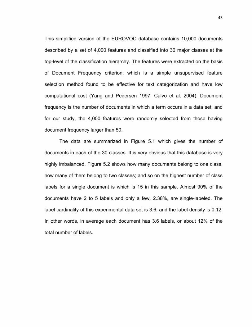
This simplified version of the EUROVOC database contains 10,000 documents
described by a set of 4,000 features and classified into 30 major classes at the
top-level of the classification hierarchy. The features were extracted on the basis
of Document Frequency criterion, which is a simple unsupervised feature
selection method found to be effective for text categorization and have low
computational cost (Yang and Pedersen 1997; Calvo et al. 2004). Document
frequency is the number of documents in which a term occurs in a data set, and
for our study, the 4,000 features were randomly selected from those having
document frequency larger than 50.
The data are summarized in Figure 5.1 which gives the number of
documents in each of the 30 classes. It is very obvious that this database is very
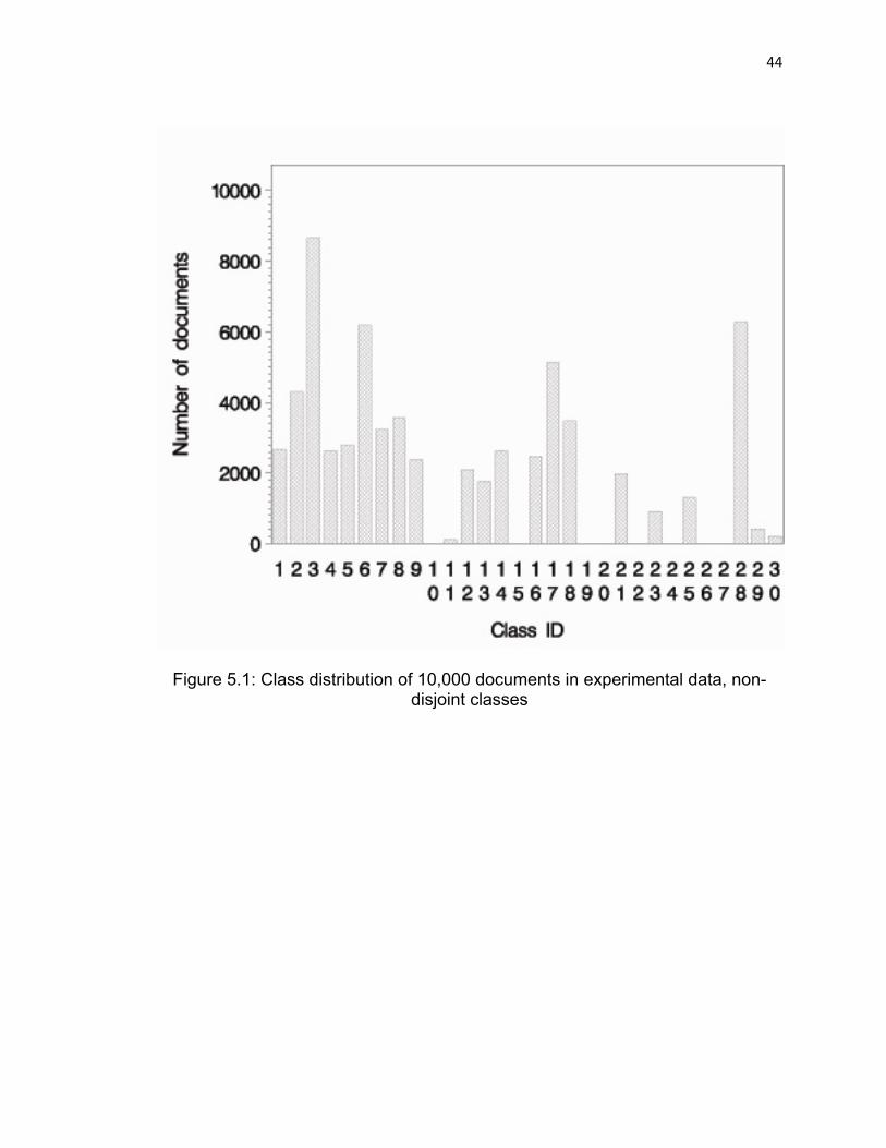
highly imbalanced. Figure 5.2 shows how many documents belong to one class,
how many of them belong to two classes; and so on the highest number of class
labels for a single document is which is 15 in this sample. Almost 90% of the
documents have 2 to 5 labels and only a few, 2.38%, are single-labeled. The
label cardinality of this experimental data set is 3.6, and the label density is 0.12.
In other words, in average each document has 3.6 labels, or about 12% of the
total number of labels.
44
Figure 5.1: Class distribution of 10,000 documents in experimental data, non-disjoint classes
45
Figure 5.2: Number of documents in the experimental data having different number of class labels
5.2 Multi-label C4.5 Results
In this project, we mostly worked on the multi-label C4.5 algorithm. Table
5.1 shows the results of our experiments when we used the multi-label C4.5
algorithm on our dataset. This table shows the F-Macro and F-Micro values
which we used as our performance criteria and it also includes the information
46
about the total CPU time which let us have a better idea about the performance
of this algorithm for different number of features.
The first three values that we can see on the table are the experiments
with the original data which has 500, 1000, and 2000 features. As we can see on
the table, running 2000 features usually takes more than four times of running
500 features. However, F-Micro and F-Macro values are higher for the big data.
At this point, the thing that we want to do is to find the minimum possible CPU
time with the maximum possible accuracy at the same time.
When we divide the 2000 feature dataset by two which we can see at the
4th and 5th row, we will see that the average CPU time of running the same data
is 24.5 minutes which is almost the same with running the 1000 features at the
same time. When we compare those two F-Micro and F-Macro values, we will
see that there is no major difference on the accuracies and the performance of
the system is doubled since it takes half time of running the experiment on 2000
features at the same time.
In the following table, we can also compare the performances of running
the same data by dividing the features into four and eight parts. When we divide
the 2000 feature dataset by four and run the same algorithm on every 500
feature dataset, we will see that the average time to run the data is only 7.75
minutes. It sounds good to run the same data in 7.75 minutes instead of 42
minutes but as we know, there is one more criteria that we need to deal with
which is the accuracy. There is a major difference when we divide the 2000
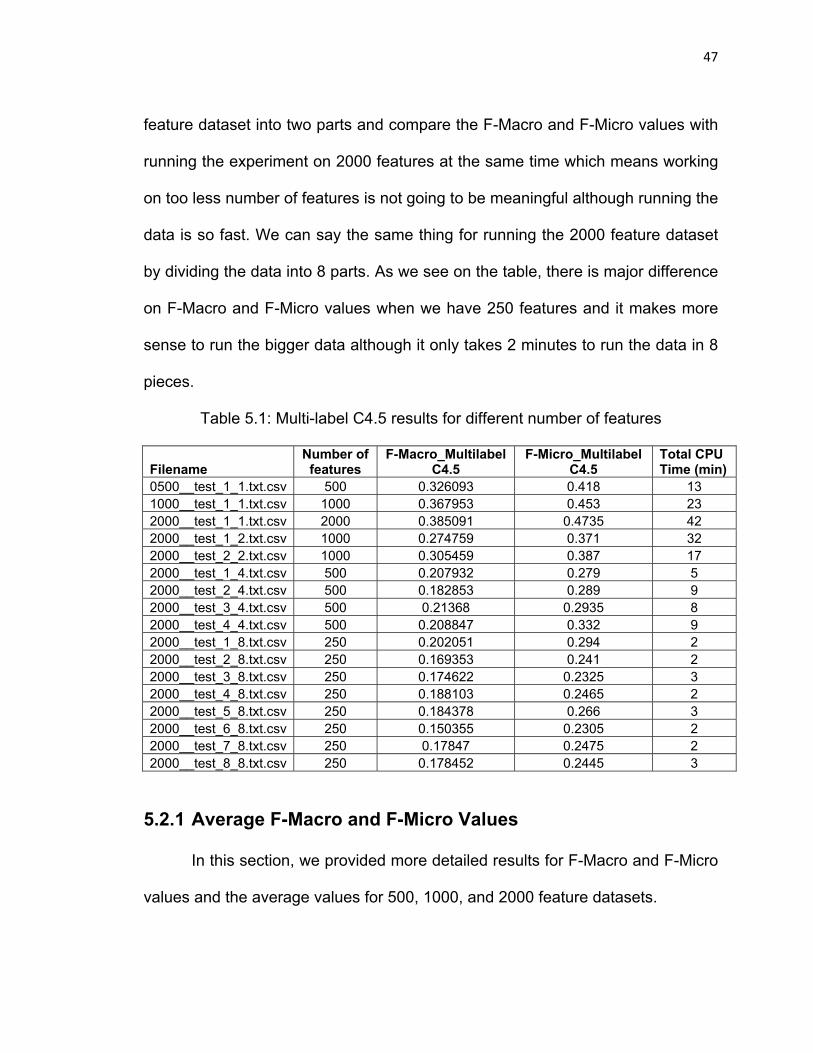
47
feature dataset into two parts and compare the F-Macro and F-Micro values with
running the experiment on 2000 features at the same time which means working
on too less number of features is not going to be meaningful although running the
data is so fast. We can say the same thing for running the 2000 feature dataset
by dividing the data into 8 parts. As we see on the table, there is major difference
on F-Macro and F-Micro values when we have 250 features and it makes more
sense to run the bigger data although it only takes 2 minutes to run the data in 8
pieces.
Table 5.1: Multi-label C4.5 results for different number of features
Filename Number of
features F-Macro_Multilabel
C4.5 F-Micro_Multilabel
C4.5 Total CPU Time (min)
0500__test_1_1.txt.csv 500 0.326093 0.418 13 1000__test_1_1.txt.csv 1000 0.367953 0.453 23 2000__test_1_1.txt.csv 2000 0.385091 0.4735 42 2000__test_1_2.txt.csv 1000 0.274759 0.371 32 2000__test_2_2.txt.csv 1000 0.305459 0.387 17 2000__test_1_4.txt.csv 500 0.207932 0.279 5 2000__test_2_4.txt.csv 500 0.182853 0.289 9 2000__test_3_4.txt.csv 500 0.21368 0.2935 8 2000__test_4_4.txt.csv 500 0.208847 0.332 9 2000__test_1_8.txt.csv 250 0.202051 0.294 2 2000__test_2_8.txt.csv 250 0.169353 0.241 2 2000__test_3_8.txt.csv 250 0.174622 0.2325 3 2000__test_4_8.txt.csv 250 0.188103 0.2465 2 2000__test_5_8.txt.csv 250 0.184378 0.266 3 2000__test_6_8.txt.csv 250 0.150355 0.2305 2 2000__test_7_8.txt.csv 250 0.17847 0.2475 2 2000__test_8_8.txt.csv 250 0.178452 0.2445 3
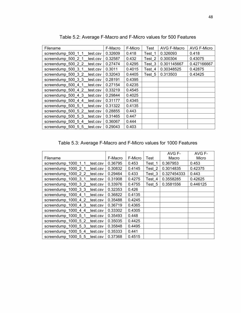
5.2.1 Average F-Macro and F-Micro Values
In this section, we provided more detailed results for F-Macro and F-Micro
values and the average values for 500, 1000, and 2000 feature datasets.
48
Table 5.2: Average F-Macro and F-Micro values for 500 Features
Filename F-Macro F-Micro Test AVG F-Macro AVG F-Micro screendump_500_1_1__test.csv 0.32609 0.418 Test_1 0.326093 0.418 screendump_500_2_1__test.csv 0.32587 0.432 Test_2 0.300304 0.43075 screendump_500_2_2__test.csv 0.27474 0.4295 Test_3 0.301145667 0.427166667screendump_500_3_1__test.csv 0.3011 0.4015 Test_4 0.30348525 0.42875 screendump_500_3_2__test.csv 0.32043 0.4405 Test_5 0.313503 0.43425 screendump_500_3_3__test.csv 0.28191 0.4395 screendump_500_4_1__test.csv 0.27154 0.4235 screendump_500_4_2__test.csv 0.33219 0.4545 screendump_500_4_3__test.csv 0.29844 0.4025 screendump_500_4_4__test.csv 0.31177 0.4345 screendump_500_5_1__test.csv 0.31322 0.4135 screendump_500_5_2__test.csv 0.28855 0.443 screendump_500_5_3__test.csv 0.31465 0.447 screendump_500_5_4__test.csv 0.36067 0.444 screendump_500_5_5__test.csv 0.29043 0.403
Table 5.3: Average F-Macro and F-Micro values for 1000 Features
Filename F-Macro F-Micro Test AVG F-Macro
AVG F-Micro
screendump_1000_1_1__test.csv 0.36795 0.453 Test_1 0.367953 0.453 screendump_1000_2_1__test.csv 0.30832 0.4145 Test_2 0.3014835 0.42375 screendump_1000_2_2__test.csv 0.29464 0.433 Test_3 0.327454333 0.443 screendump_1000_3_1__test.csv 0.31908 0.4275 Test_4 0.3558285 0.42625 screendump_1000_3_2__test.csv 0.33976 0.4755 Test_5 0.3581556 0.446125 screendump_1000_3_3__test.csv 0.32353 0.426 screendump_1000_4_1__test.csv 0.36822 0.4135 screendump_1000_4_2__test.csv 0.35488 0.4245 screendump_1000_4_3__test.csv 0.36719 0.4365 screendump_1000_4_4__test.csv 0.33302 0.4305 screendump_1000_5_1__test.csv 0.35493 0.448 screendump_1000_5_2__test.csv 0.35035 0.4425 screendump_1000_5_3__test.csv 0.35848 0.4495 screendump_1000_5_4__test.csv 0.35333 0.441 screendump_1000_5_5__test.csv 0.37368 0.4515
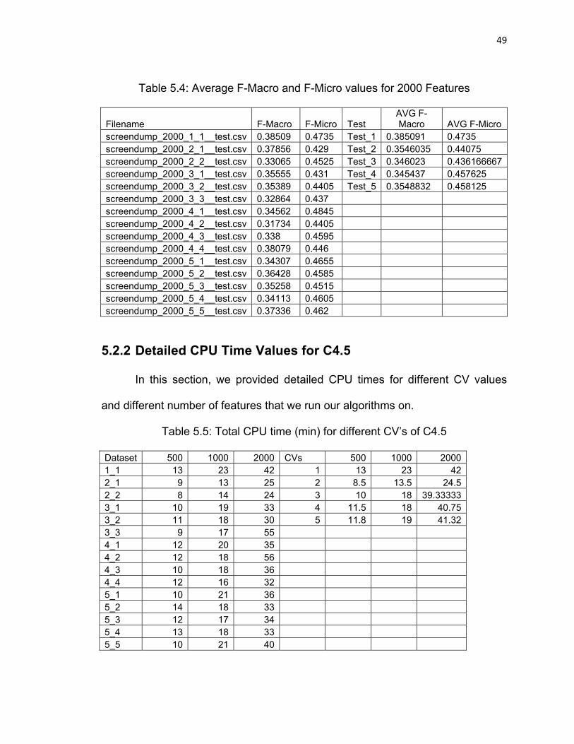
49
Table 5.4: Average F-Macro and F-Micro values for 2000 Features
Filename F-Macro F-Micro Test AVG F-Macro AVG F-Micro
screendump_2000_1_1__test.csv 0.38509 0.4735 Test_1 0.385091 0.4735 screendump_2000_2_1__test.csv 0.37856 0.429 Test_2 0.3546035 0.44075 screendump_2000_2_2__test.csv 0.33065 0.4525 Test_3 0.346023 0.436166667screendump_2000_3_1__test.csv 0.35555 0.431 Test_4 0.345437 0.457625 screendump_2000_3_2__test.csv 0.35389 0.4405 Test_5 0.3548832 0.458125 screendump_2000_3_3__test.csv 0.32864 0.437 screendump_2000_4_1__test.csv 0.34562 0.4845 screendump_2000_4_2__test.csv 0.31734 0.4405 screendump_2000_4_3__test.csv 0.338 0.4595 screendump_2000_4_4__test.csv 0.38079 0.446 screendump_2000_5_1__test.csv 0.34307 0.4655 screendump_2000_5_2__test.csv 0.36428 0.4585 screendump_2000_5_3__test.csv 0.35258 0.4515 screendump_2000_5_4__test.csv 0.34113 0.4605 screendump_2000_5_5__test.csv 0.37336 0.462
5.2.2 Detailed CPU Time Values for C4.5
In this section, we provided detailed CPU times for different CV values
and different number of features that we run our algorithms on.
Table 5.5: Total CPU time (min) for different CV’s of C4.5
Dataset 500 1000 2000 CVs 500 1000 2000 1_1 13 23 42 1 13 23 42 2_1 9 13 25 2 8.5 13.5 24.5 2_2 8 14 24 3 10 18 39.33333 3_1 10 19 33 4 11.5 18 40.75 3_2 11 18 30 5 11.8 19 41.32 3_3 9 17 55 4_1 12 20 35 4_2 12 18 56 4_3 10 18 36 4_4 12 16 32 5_1 10 21 36 5_2 14 18 33 5_3 12 17 34 5_4 13 18 33 5_5 10 21 40
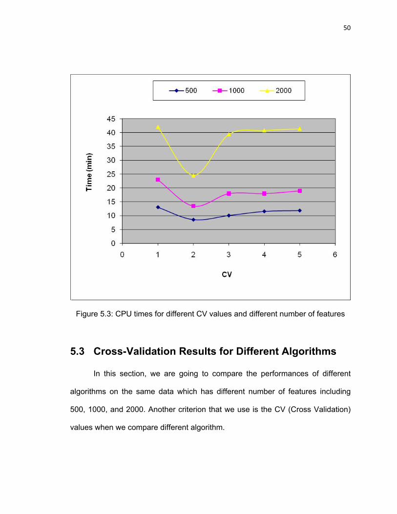
50
Figure 5.3: CPU times for different CV values and different number of features
5.3 Cross-Validation Results for Different Algorithms
In this section, we are going to compare the performances of different
algorithms on the same data which has different number of features including
500, 1000, and 2000. Another criterion that we use is the CV (Cross Validation)
values when we compare different algorithm.
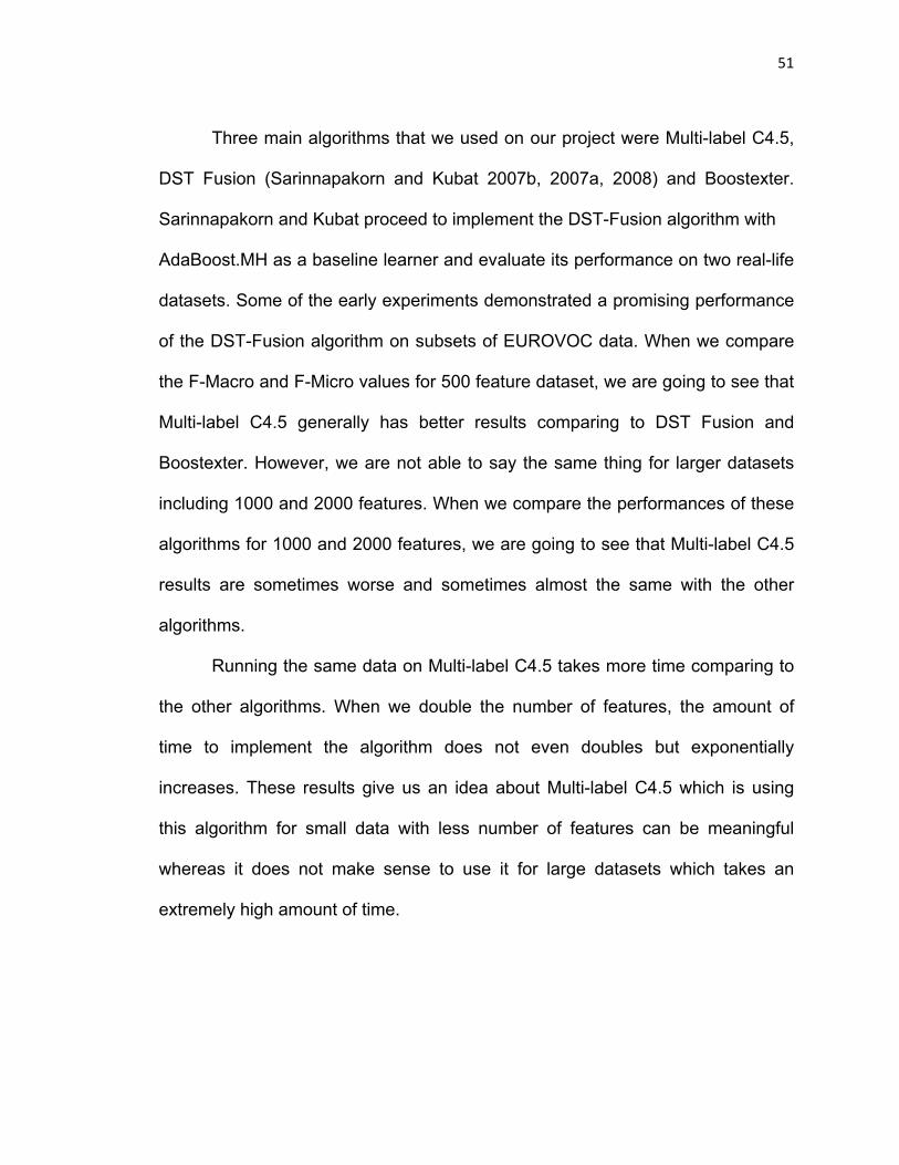
51
Three main algorithms that we used on our project were Multi-label C4.5,
DST Fusion (Sarinnapakorn and Kubat 2007b, 2007a, 2008) and Boostexter.
Sarinnapakorn and Kubat proceed to implement the DST-Fusion algorithm with
AdaBoost.MH as a baseline learner and evaluate its performance on two real-life
datasets. Some of the early experiments demonstrated a promising performance
of the DST-Fusion algorithm on subsets of EUROVOC data. When we compare
the F-Macro and F-Micro values for 500 feature dataset, we are going to see that
Multi-label C4.5 generally has better results comparing to DST Fusion and
Boostexter. However, we are not able to say the same thing for larger datasets
including 1000 and 2000 features. When we compare the performances of these
algorithms for 1000 and 2000 features, we are going to see that Multi-label C4.5
results are sometimes worse and sometimes almost the same with the other
algorithms.
Running the same data on Multi-label C4.5 takes more time comparing to
the other algorithms. When we double the number of features, the amount of
time to implement the algorithm does not even doubles but exponentially
increases. These results give us an idea about Multi-label C4.5 which is using
this algorithm for small data with less number of features can be meaningful
whereas it does not make sense to use it for large datasets which takes an
extremely high amount of time.
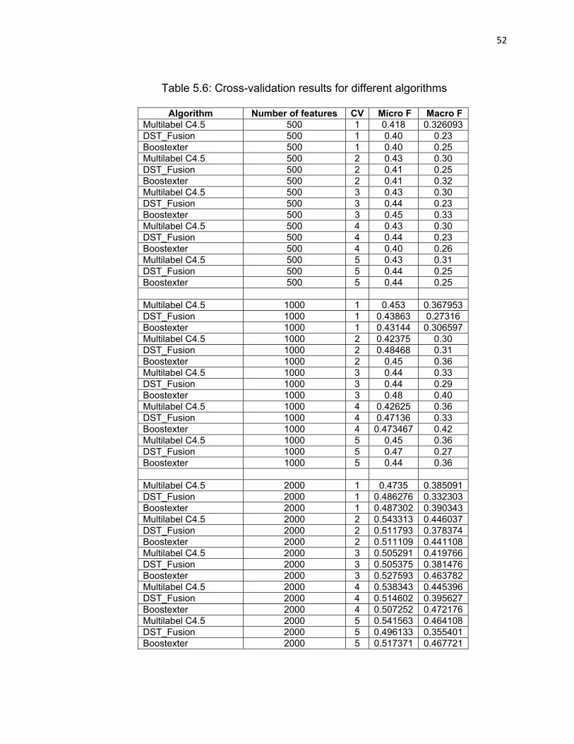
52
Table 5.6: Cross-validation results for different algorithms
Algorithm Number of features CV Micro F Macro F Multilabel C4.5 500 1 0.418 0.326093DST_Fusion 500 1 0.40 0.23 Boostexter 500 1 0.40 0.25 Multilabel C4.5 500 2 0.43 0.30 DST_Fusion 500 2 0.41 0.25 Boostexter 500 2 0.41 0.32 Multilabel C4.5 500 3 0.43 0.30 DST_Fusion 500 3 0.44 0.23 Boostexter 500 3 0.45 0.33 Multilabel C4.5 500 4 0.43 0.30 DST_Fusion 500 4 0.44 0.23 Boostexter 500 4 0.40 0.26 Multilabel C4.5 500 5 0.43 0.31 DST_Fusion 500 5 0.44 0.25 Boostexter 500 5 0.44 0.25 Multilabel C4.5 1000 1 0.453 0.367953DST_Fusion 1000 1 0.43863 0.27316 Boostexter 1000 1 0.43144 0.306597Multilabel C4.5 1000 2 0.42375 0.30 DST_Fusion 1000 2 0.48468 0.31 Boostexter 1000 2 0.45 0.36 Multilabel C4.5 1000 3 0.44 0.33 DST_Fusion 1000 3 0.44 0.29 Boostexter 1000 3 0.48 0.40 Multilabel C4.5 1000 4 0.42625 0.36 DST_Fusion 1000 4 0.47136 0.33 Boostexter 1000 4 0.473467 0.42 Multilabel C4.5 1000 5 0.45 0.36 DST_Fusion 1000 5 0.47 0.27 Boostexter 1000 5 0.44 0.36 Multilabel C4.5 2000 1 0.4735 0.385091DST_Fusion 2000 1 0.486276 0.332303Boostexter 2000 1 0.487302 0.390343Multilabel C4.5 2000 2 0.543313 0.446037DST_Fusion 2000 2 0.511793 0.378374Boostexter 2000 2 0.511109 0.441108Multilabel C4.5 2000 3 0.505291 0.419766DST_Fusion 2000 3 0.505375 0.381476Boostexter 2000 3 0.527593 0.463782Multilabel C4.5 2000 4 0.538343 0.445396DST_Fusion 2000 4 0.514602 0.395627Boostexter 2000 4 0.507252 0.472176Multilabel C4.5 2000 5 0.541563 0.464108DST_Fusion 2000 5 0.496133 0.355401Boostexter 2000 5 0.517371 0.467721
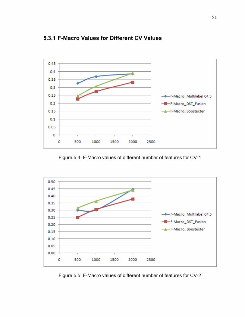
53
5.3.1 F-Macro Values for Different CV Values
Figure 5.4: F-Macro values of different number of features for CV-1
Figure 5.5: F-Macro values of different number of features for CV-2
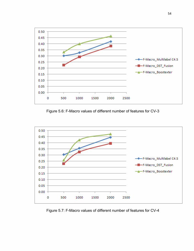
54
Figure 5.6: F-Macro values of different number of features for CV-3
Figure 5.7: F-Macro values of different number of features for CV-4
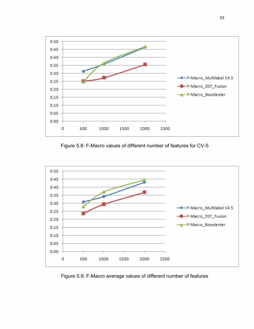
55
Figure 5.8: F-Macro values of different number of features for CV-5
Figure 5.9: F-Macro average values of different number of features
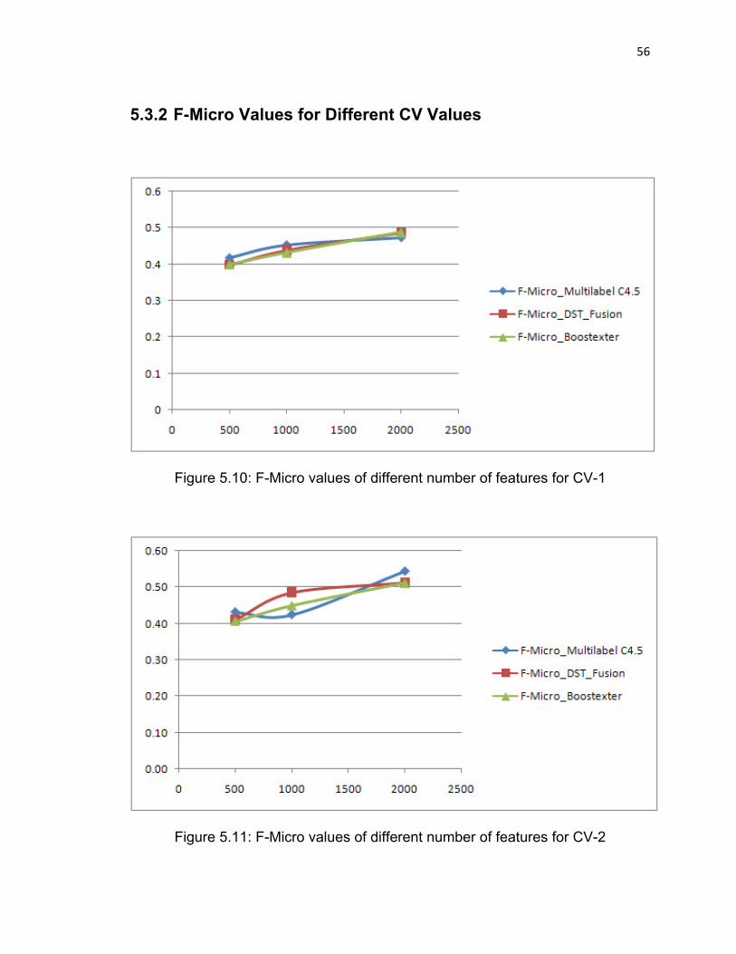
56
5.3.2 F-Micro Values for Different CV Values
Figure 5.10: F-Micro values of different number of features for CV-1
Figure 5.11: F-Micro values of different number of features for CV-2
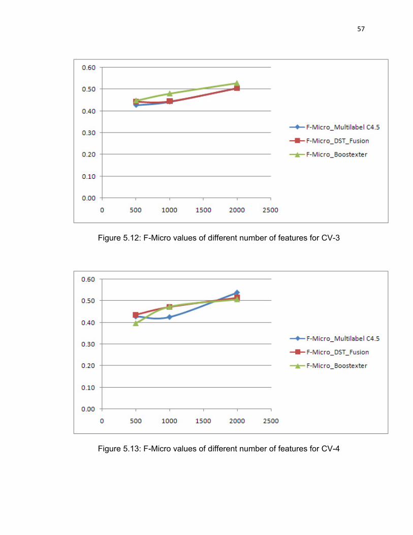
57
Figure 5.12: F-Micro values of different number of features for CV-3
Figure 5.13: F-Micro values of different number of features for CV-4
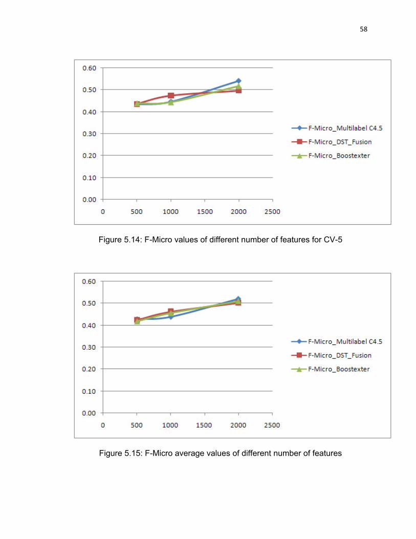
58
Figure 5.14: F-Micro values of different number of features for CV-5
Figure 5.15: F-Micro average values of different number of features
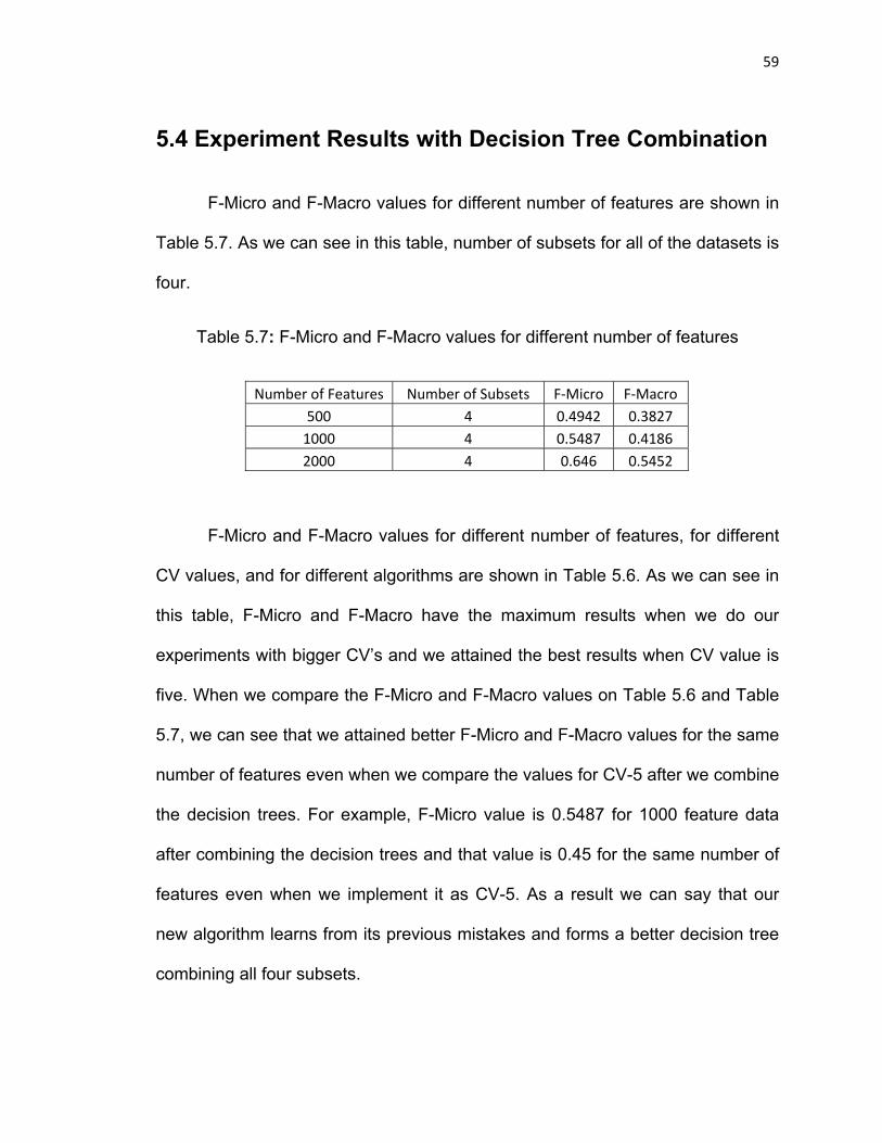
59
5.4 Experiment Results with Decision Tree Combination
F-Micro and F-Macro values for different number of features are shown in
Table 5.7. As we can see in this table, number of subsets for all of the datasets is
four.
Table 5.7: F-Micro and F-Macro values for different number of features
Number of Features Number of Subsets F‐Micro F‐Macro 500 4 0.4942 0.3827 1000 4 0.5487 0.4186 2000 4 0.646 0.5452
F-Micro and F-Macro values for different number of features, for different
CV values, and for different algorithms are shown in Table 5.6. As we can see in
this table, F-Micro and F-Macro have the maximum results when we do our
experiments with bigger CV’s and we attained the best results when CV value is
five. When we compare the F-Micro and F-Macro values on Table 5.6 and Table
5.7, we can see that we attained better F-Micro and F-Macro values for the same
number of features even when we compare the values for CV-5 after we combine
the decision trees. For example, F-Micro value is 0.5487 for 1000 feature data
after combining the decision trees and that value is 0.45 for the same number of
features even when we implement it as CV-5. As a result we can say that our
new algorithm learns from its previous mistakes and forms a better decision tree
combining all four subsets.
CHAPTER 6
Conclusions and Future Work
In this project, we used different algorithms for multi-label classification
and we compared their performances by the criteria that we described at Chapter
2. The most frequently used algorithm in this project was multi-label C4.5 and we
had a chance to compare its performance with the other famous boosting
algorithm. Boostexter was one of the boosting algorithms that we used on this
project to compare with multi-label C4.5. In this project, we saw that C4.5 has
better results comparing to the other algorithms especially for smaller datasets.
We also practiced that the biggest problem with C4.5 is the speed of running the
algorithm since it was extremely slow comparing to Boostexter on the same data
with the same number of features.
We proposed a method to solve the speed problem of C4.5 on this project
which is dividing the data by the number of features and running the same data
with smaller number of features. We got very reasonable results especially when
we divide the data into two parts by the number of features and run the data on
60

61
C4.5. F-Micro and F-Macro results which we used as our performance criteria
were very close to the original dataset when we run the same algorithm into two
parts of the same data which makes the computational cost half of running the
data completely at the same time and the results were very reasonable. We also
tried to run the same algorithm on smaller number of features of the same data
but we did not get reasonable results for smaller number of features since there
was a big difference on F-Micro and F-Macro values when we compared with the
original dataset’s results.
Based on our experience with all of these experiments, we decided that it
will be meaningful to use multi-label C4.5 especially for smaller datasets since
we got better results comparing to Boostexter and other algorithms on small
amount of features.
The last step of our project was to combine the decision trees with a
method described by Kim (2001). Kim introduced a decision tree combining
method which has better results comparing to the famous decision tree
combining methods; Bagging method, M-method, and Stacking method. This
new method uses cross-validation or bootstrap as a re-sampling technique and
discretization as a combining method and achieved better prediction accuracy
than a single decision tree algorithm. We implemented the same decision tree
combination algorithm for our project to combine the decision trees. Our
algorithm was basically checking all elements which did not belong to the
corresponding class and tried to generate rules to learn depending on its

62
previous mistakes. Our algorithm looks for best possible improvement and
calculates correction rules and we got very reasonable improvement when we
implemented this algorithm on our project in the sense of fixing the
misclassifications.
We were able to finish the experiments and got the results in a timely
manner since we used a computer which has eight processors. In this project, we
tried to improve the performances of existing algorithms by different experiments
and we got reasonable results on our studies. However, it is not possible to say
that this performance improvement or the method that we proposed to solve the
computational cost problem of multi-label C4.5 is enough since the same
experiments still take months to run especially on a regular computer. The
algorithms that we used have the highest performances all over the multi-label
classification algorithms but on a huge data collection like EUROVOC which we
used for our experiments, they are still so weak and so far of being high
performance algorithms in this case. As a result, we can say that there is still a
long way to take to improve these multi-label classification algorithms especially
when they are used on a huge dataset with many classes and features.
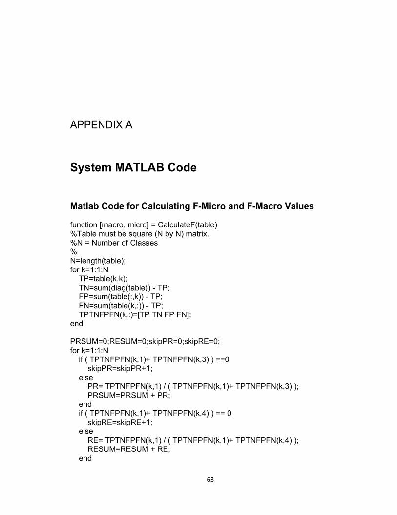
APPENDIX A
System MATLAB Code
Matlab Code for Calculating F-Micro and F-Macro Values function [macro, micro] = CalculateF(table) %Table must be square (N by N) matrix. %N = Number of Classes % N=length(table); for k=1:1:N TP=table(k,k); TN=sum(diag(table)) - TP; FP=sum(table(:,k)) - TP; FN=sum(table(k,:)) - TP; TPTNFPFN(k,:)=[TP TN FP FN]; end PRSUM=0;RESUM=0;skipPR=0;skipRE=0; for k=1:1:N if ( TPTNFPFN(k,1)+ TPTNFPFN(k,3) ) ==0 skipPR=skipPR+1; else PR= TPTNFPFN(k,1) / ( TPTNFPFN(k,1)+ TPTNFPFN(k,3) ); PRSUM=PRSUM + PR; end if ( TPTNFPFN(k,1)+ TPTNFPFN(k,4) ) == 0 skipRE=skipRE+1; else RE= TPTNFPFN(k,1) / ( TPTNFPFN(k,1)+ TPTNFPFN(k,4) ); RESUM=RESUM + RE; end
63
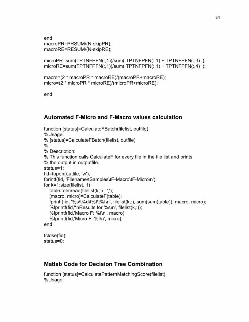
64
end macroPR=PRSUM/(N-skipPR); macroRE=RESUM/(N-skipRE); microPR=sum(TPTNFPFN(:,1))/sum( TPTNFPFN(:,1) + TPTNFPFN(:,3) ); microRE=sum(TPTNFPFN(:,1))/sum( TPTNFPFN(:,1) + TPTNFPFN(:,4) ); macro=(2 * macroPR * macroRE)/(macroPR+macroRE); micro=(2 * microPR * microRE)/(microPR+microRE); end Automated F-Micro and F-Macro values calculation function [status]=CalculateFBatch(filelist, outfile) %Usage: % [status]=CalculateFBatch(filelist, outfile) % % Description: % This function calls CalculateF for every file in the file list and prints % the output in outputfile. status=1; fid=fopen(outfile, 'w'); fprintf(fid, 'Filename\tSamples\tF-Macro\tF-Micro\n'); for k=1:size(filelist, 1) table=dlmread(filelist(k,:) , ','); [macro, micro]=CalculateF(table); fprintf(fid, '%s\t%d\t%f\t%f\n', filelist(k,:), sum(sum(table)), macro, micro); %fprintf(fid,'\nResults for %s\n', filelist(k,:)); %fprintf(fid,'Macro F: %f\n', macro); %fprintf(fid,'Micro F: %f\n', micro); end fclose(fid); status=0; Matlab Code for Decision Tree Combination function [status]=CalculatePatternMatchingScore(filelist) %Usage:
65
% [status]=CalculatePatternMatchingScore(filelist, outfile) % % Description: % This function calculates the pattern matching score for every possible pattern for each class, % and outputs it to a file... status=1; % fid=fopen(outfile, 'w'); %fprintf(fid, 'Filename\tSamples\tF-Macro\tF-Micro\n'); for k=1:size(filelist, 1) trees(k).table=dlmread(filelist(k,:) , ','); end numofclasses=size(trees(1).table,1); numoftrees=4; % ONLY 4 SUBSETS ALLOWED %numrules=0; % Rule counter %maxrules=1000; % Maximum Rules %rules=zeros(5,maxrules); %Genereate Rules Matrix 4Classes+1Value for 30^4 permutations... rules=sparse(numofclasses^numoftrees,1); %for each actual class for a=1:numofclasses %for eachtree for t=1:numoftrees %get that actual class from each tree p(t).index=find(trees(t).table(a,:) > 0); %Get nonzero classifications and indexes end %for each nonzero-class in each tree for c1=1:length(p(1).index) %get first nonzero for c2=1:length(p(2).index) for c3=1:length(p(3).index) for c4=1:length(p(4).index) V=trees(1).table(a,p(1).index(c1)) + trees(2).table(a,p(2).index(c2)) + trees(3).table(a,p(3).index(c3)) + trees(4).table(a,p(4).index(c4)) ;
66
rules_index=30^3*(p(1).index(c1)-1)+ 30^2*(p(2).index(c2)-1) + 30*(p(3).index(c3)-1) + p(4).index(c4); if rules(rules_index) < V rules(rules_index) = a; % Found new rule! end end end end end disp(a) end save rules rules %fclose(fid); status=0;
APPENDIX B
Code Update of Multi-label C4.5 (Clare 2003)
C4.5 Main Routine
/*************************************************************************/ /* */ /* Main routine, c4.5 */ /* ------------------ */ /* */ /*************************************************************************/ #include "defns.i" #include "types.i" /* External data, described in extern.i */ int MaxAtt; short MaxClass, MaxDiscrVal = 2; ItemNo MaxItem; Description *Item; DiscrValue *MaxAttVal; char *SpecialStatus; String *ClassName,
67
68
*AttName, **AttValName, FileName = "DF"; short VERBOSITY = 0, TRIALS = 10; Boolean GAINRATIO = true, SUBSET = false, BATCH = true, UNSEENS = false, PROBTHRESH = false; ItemNo MINOBJS = 2, WINDOW = 0, INCREMENT = 0; float CF = 0.25; Tree *Pruned; Boolean AllKnown = true; main(Argc, Argv) /* ---- */ int Argc; char *Argv[]; { int o; extern char *optarg; extern int optind; Boolean FirstTime=true; short Best, BestTree(); PrintHeader("decision tree generator"); /* Process options */ while ( (o = getopt(Argc, Argv, "f:bupv:t:w:i:gsm:c:")) != EOF ) { if ( FirstTime ) { printf("\n Options:\n");
69
FirstTime = false; } switch (o) { case 'f': FileName = optarg; printf("\tFile stem <%s>\n", FileName); break; case 'b': BATCH = true; printf("\tWindowing disabled (now the default)\n"); break; case 'u': UNSEENS = true; printf("\tTrees evaluated on unseen cases\n"); break; case 'p': PROBTHRESH = true; printf("\tProbability thresholds used\n"); break; case 'v': VERBOSITY = atoi(optarg); printf("\tVerbosity level %d\n", VERBOSITY); break; case 't': TRIALS = atoi(optarg); printf("\tWindowing enabled with %d trials\n", TRIALS); Check(TRIALS, 1, 10000); BATCH = false; break; case 'w': WINDOW = atoi(optarg); printf("\tInitial window size of %d items\n", WINDOW); Check(WINDOW, 1, 1000000); BATCH = false; break; case 'i': INCREMENT = atoi(optarg); printf("\tMaximum window increment of %d items\n", INCREMENT); Check(INCREMENT, 1, 1000000); BATCH = false; break; case 'g': GAINRATIO = false; printf("\tGain criterion used\n"); break; case 's': SUBSET = true; printf("\tTests on discrete attribute groups\n"); break; case 'm': MINOBJS = atoi(optarg); printf("\tSensible test requires 2 branches with >=%d cases\n",
70
MINOBJS); Check(MINOBJS, 1, 1000000); break; case 'c': CF = atof(optarg); printf("\tPruning confidence level %g%%\n", CF); Check(CF, Epsilon, 100); CF /= 100; break; case '?': printf("unrecognised option\n"); exit(1); } } /* Initialise */ GetNames(); GetData(".data"); printf("\nRead %d cases (%d attributes) from %s.data\n", MaxItem+1, MaxAtt+1, FileName); /* Build decision trees */ if ( BATCH ) { TRIALS = 1; OneTree(); Best = 0; } else { Best = BestTree(); } /* Soften thresholds in best tree */ if ( PROBTHRESH ) { printf("Softening thresholds"); if ( ! BATCH ) printf(" for best tree from trial %d", Best); printf("\n"); SoftenThresh(Pruned[Best]); printf("\n"); PrintTree(Pruned[Best]); }
71
/* Save best tree */ if ( BATCH || TRIALS == 1 ) { printf("\nTree saved\n"); } else { printf("\nBest tree from trial %d saved\n", Best); } SaveTree(Pruned[Best], ".tree"); /* Evaluation */ PrintHeader("Starting Evaluation on Training Data"); printf("\n\nEvaluation on training data (%d items):\n", MaxItem+1); // Evaluate(false, Best); Evaluate(true, Best); //Print ConfMat if ( UNSEENS ) { GetData(".test"); printf("\nEvaluation on test data (%d items):\n", MaxItem+1); Evaluate(true, Best); } PrintHeader("decision tree generator complete."); exit(0); }
Main Routine for Constructing Sets of Production Rules
/*************************************************************************/ /* */ /* Main routine for constructing sets of production rules from trees */ /* ----------------------------------------------------------------- */ /* */ /*************************************************************************/ #include "defns.i"
72
#include "types.i" /* External data. Note: uncommented variables have the same meaning as for decision trees */ int MaxAtt; short MaxClass, MaxDiscrVal; ItemNo MaxItem; Description *Item; DiscrValue *MaxAttVal; char *SpecialStatus; String *ClassName, *AttName, **AttValName, FileName = "DF"; short VERBOSITY = 0, TRIALS; Boolean UNSEENS = false, SIGTEST = false, /* use significance test in rule pruning */ SIMANNEAL = false; /* use simulated annealing */ float SIGTHRESH = 0.05, CF = 0.25, REDUNDANCY = 1.0; /* factor that guesstimates the amount of redundancy and irrelevance in the attributes */ PR *Rule; /* current rules */ RuleNo NRules = 0, /* number of current rules */ *RuleIndex; /* rule index */ short RuleSpace = 0; /* space allocated for rules */ ClassNo DefaultClass; /* current default class */
73
RuleSet *PRSet; /* sets of rulesets */ float AttTestBits, /* bits to encode tested att */ *BranchBits; /* ditto attribute value */ main(Argc, Argv) /* ---- */ int Argc; char *Argv[]; { int o; extern char *optarg; extern int optind; Boolean FirstTime=true; PrintHeader("rule generator"); /* Process options */ while ( (o = getopt(Argc, Argv, "f:uv:c:r:F:a")) != EOF ) { if ( FirstTime ) { printf("\n Options:\n"); FirstTime = false; } switch (o) { case 'f': FileName = optarg; printf("\tFile stem <%s>\n", FileName); break; case 'u': UNSEENS = true; printf("\tRulesets evaluated on unseen cases\n"); break; case 'v': VERBOSITY = atoi(optarg); printf("\tVerbosity level %d\n", VERBOSITY); break; case 'c': CF = atof(optarg); printf("\tPruning confidence level %g%%\n", CF); Check(CF, 0, 100); CF /= 100;
74
break; case 'r': REDUNDANCY = atof(optarg); printf("\tRedundancy factor %g\n", REDUNDANCY); Check(REDUNDANCY, 0, 10000); break; case 'F': SIGTHRESH = atof(optarg); printf("\tSignificance test in rule pruning, "); printf("threshold %g%%\n", SIGTHRESH); Check(SIGTHRESH, 0, 100); SIGTHRESH /= 100; SIGTEST = true; break; case 'a': SIMANNEAL = true; printf("\tSimulated annealing for selecting rules\n"); break; case '?': printf("unrecognised option\n"); exit(1); } } /* Initialise */ GetNames(); GetData(".data"); printf("\nRead %d cases (%d attributes) from %s\n", MaxItem+1, MaxAtt+1, FileName); GenerateLogs(); printf("Completed: Generate Logs. Starting Generate Rules.\n"); /* Construct rules */ GenerateRules(); printf("Completed: Generate Rules. Starting Generate Evaluations.\n"); /* Evaluations */ printf("\n\nEvaluation on training data (%d items):\n", MaxItem+1); EvaluateRulesets(true); printf("Completed: Training Evaluations. Saving Rules.\n"); /* Save current ruleset */ SaveRules();
75
if ( UNSEENS ) { GetData(".test"); printf("\nEvaluation on test data (%d items):\n", MaxItem+1); EvaluateRulesets(false); } printf("Completed: Evaluating Test Data. Exiting.\n"); exit(0); } Average Results for Training and Testing Sets
/*************************************************************************/ /* */ /* Average results for training and test sets */ /* ------------------------------------------ */ /* */ /* This is a generic program that averages any numbers found on */ /* a set of lines of the same pattern. */ /* */ /*************************************************************************/ #include <stdio.h> #define MAXLINE 200 /* max line length */ #define MAXVALS 10 /* max values to be averaged */ main() { char Line[MAXLINE], *p1, *p2; int Numbers=0, Lines=0, i, TrainTest; float Val, Sum[2][MAXVALS]; double strtod(); for ( i = 0 ; i < MAXVALS ; i++ ) { Sum[0][i] = Sum[1][i] = 0; } while ( fgets(Line, MAXLINE, stdin) )
76
{ i = 0; TrainTest = Lines % 2; printf("%s", Line); /* Count the numbers appearing on the line */ for ( p1 = Line ; *p1 != '\n' ; p1++ ) { if ( *p1 < '0' || *p1 > '9' ) continue; Val = strtod(p1, &p2); Sum[TrainTest][i++] += Val; p1 = p2-1; } /* The number of numbers must match any previous lines */ if ( Lines ) { if ( i != Numbers ) { exit(0); } } else { Numbers = i; } Lines++; } putchar('\n'); for ( TrainTest = 0 ; TrainTest <= 1 ; TrainTest++ ) { i = 0; printf("%s:\t", TrainTest ? "test" : "train"); for ( p1 = Line ; *p1 != '\n' ; p1++ ) { if ( *p1 < '0' || *p1 > '9' ) { putchar(*p1); }
77
else { printf("%.1f", Sum[TrainTest][i++] / (0.5 * Lines)); strtod(p1, &p2); p1 = p2-1; } } putchar('\n'); } }
Form a Set of Rules from a Decision Tree
/*************************************************************************/ /* */ /* Form a set of rules from a decision tree */ /* ---------------------------------------- */ /* */ /*************************************************************************/ #include "defns.i" #include "types.i" #include "extern.i" #include "rulex.i" ItemNo *TargetClassFreq, /* [Boolean] */ *Errors, /* [Condition] */ *Total; /* [Condition] */ float *Pessimistic, /* [Condition] */ *Actual, /* [Condition] */ *CondSigLevel; /* [Condition] */ Boolean **CondSatisfiedBy, /* [Condition][ItemNo] */ *Deleted; /* [Condition] */ DiscrValue *SingleValue; /* [Attribute] */ Condition *Stack; short MaxDisjuncts,
78
MaxDepth; short Zeynel; /*************************************************************************/ /* */ /* Form a ruleset from decision tree t */ /* */ /*************************************************************************/ FormRules(t) /* ---------- */ Tree t; { short i; /* Find essential parameters and allocate storage */ MaxDepth = 0; MaxDisjuncts = 0; TreeParameters(t, 0); Actual = (float *) calloc(MaxDepth+2, sizeof(float)); Total = (ItemNo *) calloc(MaxDepth+2, sizeof(ItemNo)); Errors = (ItemNo *) calloc(MaxDepth+2, sizeof(ItemNo)); Pessimistic = (float *) calloc(MaxDepth+2, sizeof(float)); CondSigLevel = (float *) calloc(MaxDepth+2, sizeof(float)); TargetClassFreq = (ItemNo *) calloc(2, sizeof(ItemNo)); Deleted = (Boolean *) calloc(MaxDepth+2, sizeof(Boolean)); CondSatisfiedBy = (char **) calloc(MaxDepth+2, sizeof(char *)); Stack = (Condition *) calloc(MaxDepth+2, sizeof(Condition)); ForEach(i, 0, MaxDepth+1) { CondSatisfiedBy[i] = (char *) calloc(MaxItem+1, sizeof(char)); Stack[i] = (Condition) malloc(sizeof(struct CondRec)); } SingleValue = (DiscrValue *) calloc(MaxAtt+1, sizeof(DiscrValue));
79
printf("In FormRules, Initialising Rules!\n"); InitialiseRules(); /* Extract and prune disjuncts */ Zeynel=0; printf("In FormRules, Scanning tree\n"); Scan(t, 0); printf("Scan Complete!\n"); /* Deallocate storage */ ForEach(i, 0, MaxDepth+1) { cfree(CondSatisfiedBy[i]); cfree(Stack[i]); } cfree(Deleted); cfree(CondSatisfiedBy); cfree(Stack); cfree(Actual); cfree(Total); cfree(Errors); cfree(Pessimistic); cfree(CondSigLevel); cfree(TargetClassFreq); } /*************************************************************************/ /* */ /* Find the maximum depth and the number of leaves in tree t */ /* with initial depth d */ /* */ /*************************************************************************/ TreeParameters(t, d) /* --------------- */ Tree t; short d; {
80
DiscrValue v; if ( t->NodeType ) { ForEach(v, 1, t->Forks) { TreeParameters(t->Branch[v], d+1); } } else { /* This is a leaf */ if ( d > MaxDepth ) MaxDepth = d; MaxDisjuncts++; } } /*************************************************************************/ /* */ /* Extract disjuncts from tree t at depth d, and process them */ /* */ /*************************************************************************/ Scan(t, d) /* ---- */ Tree t; short d; { DiscrValue v; short i; printf("condition\n"); Condition *Term; printf("testx \n"); Test x, FindTest(); Zeynel++; if (t == NULL) printf("t is NULL\n"); printf("Zeynel: %d - %o\n", Zeynel, t); printf("Nodetype: %d, Items %f Forks %d\n", t->NodeType, t->Items, t->Forks); if ( t->NodeType ) {
81
d++; printf("d: %d v:%d i:%d \n", d, v, i); x = (Test) malloc(sizeof(struct TestRec)); x->NodeType = t->NodeType; x->Tested = t->Tested; x->Forks = t->Forks; x->Cut = ( t->NodeType == ThreshContin ? t->Cut : 0 ); if ( t->NodeType == BrSubset ) { x->Subset = (Set *) calloc(t->Forks + 1, sizeof(Set)); ForEach(v, 1, t->Forks) { x->Subset[v] = t->Subset[v]; } } Stack[d]->CondTest = FindTest(x); ForEach(v, 1, t->Forks) { if(t->Branch[v]>0){ Stack[d]->TestValue = v; Scan(t->Branch[v], d); } printf("T-Branch[v]: %o\n", t->Branch[v]); } } else if ( t->Items >= 1 ) { /* Leaf of decision tree - construct the set of conditions associated with this leaf and prune */ Term = (Condition *) calloc(d+1, sizeof(Condition)); ForEach(i, 1, d) { Term[i] = (Condition) malloc(sizeof(struct CondRec)); Term[i]->CondTest = Stack[i]->CondTest; Term[i]->TestValue = Stack[i]->TestValue; } PruneRule(Term, d, t->LeafCount, t->Leaf); cfree(Term);
82
} printf("\t d: %d v:%d i:%d\n", d, v, i); }
Generating all Rules from the Decision Trees
/*************************************************************************/ /* */ /* Generate all rulesets from the decision trees */ /* --------------------------------------------- */ /* */ /*************************************************************************/ #include "defns.i" #include "types.i" #include "extern.i" #include "rulex.i" /*************************************************************************/ /* */ /* For each tree, form a set of rules and process them, then form a */ /* composite set of rules from all of these sets. */ /* If there is only one tree, then no composite set is formed. */ /* */ /* Rulesets are stored in PRSet[0] to PRSet[TRIALS], where */ /* PRSet[TRIALS] contains the composite ruleset. */ /* */ /* On completion, the current ruleset is the composite ruleset (if one */ /* has been made), otherwise the ruleset from the single tree. */ /* */ /*************************************************************************/ GenerateRules() /* ------------- */ { Tree DecisionTree, GetTree(); short t=0, RuleSetSpace=0, r; /* Find bits to encode attributes and branches */
83
FindTestCodes(); /* Now process each decision tree */ while ( DecisionTree = GetTree(".unpruned") ) { printf("\n------------------\n"); printf("Processing tree %d\n", t); /* Form a set of rules from the next tree */ FormRules(DecisionTree); /* Process the set of rules for this trial */ printf("Rules Formed! Constructing Ruleset!\n"); ConstructRuleset(); printf("\nFinal rules from tree %d:\n", t); PrintIndexedRules(); /* Make sure there is enough room for the new ruleset */ if ( t + 1 >= RuleSetSpace ) { RuleSetSpace += 10; if ( RuleSetSpace > 10 ) { PRSet = (RuleSet *) realloc(PRSet, RuleSetSpace * sizeof(RuleSet)); } else { PRSet = (RuleSet *) malloc(RuleSetSpace * sizeof(RuleSet)); } } PRSet[t].SNRules = NRules; PRSet[t].SRule = Rule; PRSet[t].SRuleIndex = RuleIndex; PRSet[t].SDefaultClass = DefaultClass; ++t;
84
} if ( ! t ) { printf("\nERROR: can't find any decision trees\n"); exit(1); } TRIALS = t; /* If there is more than one tree in the trees file, make a composite ruleset of the rules from all trees */ if ( TRIALS > 1 ) { CompositeRuleset(); } } /*************************************************************************/ /* */ /* Determine code lengths for attributes and branches */ /* */ /*************************************************************************/ FindTestCodes() /* ------------- */ { Attribute Att; DiscrValue v, V; ItemNo i, *ValFreq; int PossibleCuts; float Sum, SumBranches=0, p; void SwapUnweighted(); BranchBits = (float *) malloc((MaxAtt+1) * sizeof(float)); ForEach(Att, 0, MaxAtt) { if ( (V = MaxAttVal[Att]) ) {
85
ValFreq = (ItemNo *) calloc(V+1, sizeof(ItemNo)); ForEach(i, 0, MaxItem) { ValFreq[DVal(Item[i],Att)]++; } Sum = 0; ForEach(v, 1, V) { if ( ValFreq[v] ) { Sum += (ValFreq[v] / (MaxItem+1.0)) * (LogItemNo[MaxItem+1] - LogItemNo[ValFreq[v]]); } } free(ValFreq); BranchBits[Att] = Sum; } else { Quicksort(0, MaxItem, Att, SwapUnweighted); PossibleCuts = 1; ForEach(i, 1, MaxItem) { if ( CVal(Item[i],Att) > CVal(Item[i-1],Att) ) { PossibleCuts++; } } BranchBits[Att] = PossibleCuts > 1 ? 1 + LogItemNo[PossibleCuts] / 2 : 0 ; } SumBranches += BranchBits[Att]; } AttTestBits = 0; ForEach(Att, 0, MaxAtt) { if ( (p = BranchBits[Att] / SumBranches) > 0 )
86
{ AttTestBits -= p * log(p) / log(2.0); } } } /*************************************************************************/ /* */ /* Exchange items at a and b. Note: unlike the similar routine in */ /* buildtree, this does not assume that items have a Weight to be */ /* swapped as well! */ /* */ /*************************************************************************/ void SwapUnweighted(a, b) /* -------------- */ ItemNo a, b; { Description Hold; Hold = Item[a]; Item[a] = Item[b]; Item[b] = Hold; } /*************************************************************************/ /* */ /* Form composite ruleset for all trials */ /* */ /*************************************************************************/ CompositeRuleset() /* ---------------- */ { RuleNo r; short t, ri; Boolean NewRule();
87
InitialiseRules(); /* Lump together all the rules from each ruleset */ ForEach(t, 0, TRIALS-1) { ForEach(ri, 1, PRSet[t].SNRules) { r = PRSet[t].SRuleIndex[ri]; NewRule(PRSet[t].SRule[r].Lhs, PRSet[t].SRule[r].Size, PRSet[t].SRule[r].Rhs, PRSet[t].SRule[r].Error); } } /* ... and select a subset in the usual way */ ConstructRuleset(); printf("\nComposite ruleset:\n"); PrintIndexedRules(); PRSet[TRIALS].SNRules = NRules; PRSet[TRIALS].SRule = Rule; PRSet[TRIALS].SRuleIndex = RuleIndex; PRSet[TRIALS].SDefaultClass = DefaultClass; }
Routines to Manage Tree Growth, Pruning, and Evaluation
/*************************************************************************/ /* */ /* Routines to manage tree growth, pruning and evaluation */ /* ------------------------------------------------------ */ /* */ /*************************************************************************/ #include "defns.i" #include "types.i" #include "extern.i" ItemNo *TargetClassFreq; Tree *Raw;
88
extern Tree *Pruned; /*************************************************************************/ /* */ /* Grow and prune a single tree from all data */ /* */ /*************************************************************************/ OneTree() /* --------- */ { Tree FormTree(), CopyTree(); Boolean Prune(); InitialiseTreeData(); InitialiseWeights(); Raw = (Tree *) calloc(1, sizeof(Tree)); Pruned = (Tree *) calloc(1, sizeof(Tree)); AllKnown = true; Raw[0] = FormTree(0, MaxItem); printf("\n"); PrintTree(Raw[0]); /* fflush(NULL); */ SaveTree(Raw[0], ".unpruned"); Pruned[0] = CopyTree(Raw[0]); if ( Prune(Pruned[0]) ) { printf("\nSimplified "); PrintTree(Pruned[0]); } /* fflush(NULL); */ } /*************************************************************************/ /* */
89
/* Grow and prune TRIALS trees and select the best of them */ /* */ /*************************************************************************/ short BestTree() /* -------- */ { Tree CopyTree(), Iterate(); Boolean Prune(); short t, Best=0; InitialiseTreeData(); TargetClassFreq = (ItemNo *) calloc(MaxClass+1, sizeof(ItemNo)); Raw = (Tree *) calloc(TRIALS, sizeof(Tree)); Pruned = (Tree *) calloc(TRIALS, sizeof(Tree)); /* If necessary, set initial size of window to 20% (or twice the sqrt, if this is larger) of the number of data items, and the maximum number of items that can be added to the window at each iteration to 20% of the initial window size */ if ( ! WINDOW ) { WINDOW = Max(2 * sqrt(MaxItem+1.0), (MaxItem+1) / 5); } if ( ! INCREMENT ) { INCREMENT = Max(WINDOW / 5, 1); } FormTarget(WINDOW); /* Form set of trees by iteration and prune */ printf("Calculating Best Tree...\n"); ForEach(t, 0, TRIALS-1 ) { FormInitialWindow(); printf("\n--------\nTrial %d\n--------\n\n", t);
90
Raw[t] = Iterate(WINDOW, INCREMENT); printf("\n"); PrintTree(Raw[t]); SaveTree(Raw[t], ".unpruned"); Pruned[t] = CopyTree(Raw[t]); if ( Prune(Pruned[t]) ) { printf("\nSimplified "); PrintTree(Pruned[t]); } if ( Pruned[t]->Errors < Pruned[Best]->Errors ) { Best = t; } } printf("\n--------\n"); return Best; } /*************************************************************************/ /* */ /* The windowing approach seems to work best when the class */ /* distribution of the initial window is as close to uniform as */ /* possible. FormTarget generates this initial target distribution, */ /* setting up a TargetClassFreq value for each class. */ /* */ /*************************************************************************/ FormTarget(Size) /* ----------- */ ItemNo Size; { ItemNo i, *ClassFreq; ClassNo c, Smallest, ClassesLeft=0; int NoClasses, n;
91
ClassFreq = (ItemNo *) calloc(MaxClass+1, sizeof(ItemNo)); /* Generate the class frequency distribution */ ForEach(i, 0, MaxItem) { NoClasses = NumberOfClasses(Item[i]); ForEach(n, 1, NoClasses) { ClassFreq[ ClassAt(Item[i],n) ]++; } /* ClassFreq[ Class(Item[i]) ]++; */ } /* Calculate the no. of classes of which there are items */ ForEach(c, 0, MaxClass) { if ( ClassFreq[c] ) { ClassesLeft++; } else { TargetClassFreq[c] = 0; } } while ( ClassesLeft ) { /* Find least common class of which there are some items */ Smallest = -1; ForEach(c, 0, MaxClass) { if ( ClassFreq[c] && ( Smallest < 0 || ClassFreq[c] < ClassFreq[Smallest] ) ) { Smallest = c; } } /* Allocate the no. of items of this class to use in the window */
92
TargetClassFreq[Smallest] = Min(ClassFreq[Smallest], Round(Size/ClassesLeft)); ClassFreq[Smallest] = 0; Size -= TargetClassFreq[Smallest]; ClassesLeft--; } cfree(ClassFreq); } /*************************************************************************/ /* */ /* Form initial window, attempting to obtain the target class profile */ /* in TargetClassFreq. This is done by placing the targeted number */ /* of items of each class at the beginning of the set of data items. */ /* */ /*************************************************************************/ FormInitialWindow() /* ------------------- */ { ItemNo i, Start=0, More; ClassNo c; void Swap(); Shuffle(); ForEach(c, 0, MaxClass) { More = TargetClassFreq[c]; //printf("Forming Initial Window- Class: %d of %d\n%d -%d \n", c, MaxClass, Start, More); for ( i = Start ; More ; i++ ) { if( i> MaxItem) i=0; //ZSendur If number of elements are not enough go back to first element to complete the tree... if( IsInClasses( Item[i], c )) {
93
Swap(Start, i); Start++; More--; // printf("\titem: %d, %d, %d\n", i, Start, More); } } } } /*************************************************************************/ /* */ /* Shuffle the data items randomly */ /* */ /*************************************************************************/ Shuffle() /* ------- */ { ItemNo This, Alt, Left; Description Hold; This = 0; for( Left = MaxItem+1 ; Left ; ) { Alt = This + (Left--) * Random; Hold = Item[This]; Item[This++] = Item[Alt]; Item[Alt] = Hold; } } /*************************************************************************/ /* */ /* Grow a tree iteratively with initial window size Window and */ /* initial window increment IncExceptions. */ /* */ /* Construct a classifier tree using the data items in the */ /* window, then test for the successful classification of other */ /* data items by this tree. If there are misclassified items, */
94
/* put them immediately after the items in the window, increase */ /* the size of the window and build another classifier tree, and */ /* so on until we have a tree which successfully classifies all */ /* of the test items or no improvement is apparent. */ /* */ /* On completion, return the tree which produced the least errors. */ /* */ /*************************************************************************/ Tree Iterate(Window, IncExceptions) /* ------- */ ItemNo Window, IncExceptions; { Tree Classifier, BestClassifier=Nil, FormTree(); ItemNo i, Errors, TotalErrors, BestTotalErrors=MaxItem+1, Exceptions, Additions; ClassNo Assigned, Category(); short Cycle=0; void Swap(); printf("Cycle Tree -----Cases----"); printf(" -----------------Errors-----------------\n"); printf(" size window other"); printf(" window rate other rate total rate\n"); printf("----- ---- ------ ------"); printf(" ------ ---- ------ ---- ------ ----\n"); do { /* Build a classifier tree with the first Window items */ InitialiseWeights(); AllKnown = true; Classifier = FormTree(0, Window-1); /* Error analysis */ Errors = Round(Classifier->Errors); /* Move all items that are incorrectly classified by the classifier tree to immediately after the items in the current window. */
95
Exceptions = Window; ForEach(i, Window, MaxItem) { Assigned = Category(Item[i], Classifier); /* if ( Assigned != Class(Item[i]) ) */ if( ! (IsInClasses( Item[i],Assigned))) { Swap(Exceptions, i); Exceptions++; } } Exceptions -= Window; TotalErrors = Errors + Exceptions; /* Print error analysis */ printf("%3d %7d %8d %6d %8d%5.1f%% %6d%5.1f%% %6d%5.1f%%\n", ++Cycle, TreeSize(Classifier), Window, MaxItem-Window+1, Errors, 100*(float)Errors/Window, Exceptions, 100*Exceptions/(MaxItem-Window+1.001), TotalErrors, 100*TotalErrors/(MaxItem+1.0)); /* Keep track of the most successful classifier tree so far */ if ( ! BestClassifier || TotalErrors < BestTotalErrors ) { if ( BestClassifier ) ReleaseTree(BestClassifier); BestClassifier = Classifier; BestTotalErrors = TotalErrors; } else { ReleaseTree(Classifier); } /* Increment window size */ Additions = Min(Exceptions, IncExceptions); Window = Min(Window + Max(Additions, Exceptions / 2), MaxItem + 1); } while ( Exceptions ); return BestClassifier;
96
} /*************************************************************************/ /* */ /* Print report of errors for each of the trials */ /* */ /*************************************************************************/ Evaluate(CMInfo, Saved) /* -------- */ Boolean CMInfo; short Saved; { ClassNo RealClass, PrunedClass, Category(); short t; ItemNo *ConfusionMat, i, RawErrors, PrunedErrors; if ( CMInfo ) { ConfusionMat = (ItemNo *) calloc((MaxClass+1)*(MaxClass+1), sizeof(ItemNo)); } printf("\n"); if ( TRIALS > 1 ) { printf("Trial\t Before Pruning After Pruning\n"); printf("-----\t---------------- ---------------------------\n"); } else { printf("\t Before Pruning After Pruning\n"); printf("\t---------------- ---------------------------\n"); } printf("\tSize Errors Size Errors Estimate\n\n"); ForEach(t, 0, TRIALS-1) { RawErrors = PrunedErrors = 0;
97
ForEach(i, 0, MaxItem) { /* RealClass = Class(Item[i]); */ RealClass = ClassAt(Item[i],1); if ( Category(Item[i], Raw[t]) != RealClass ) RawErrors++; PrunedClass = Category(Item[i], Pruned[t]); if ( PrunedClass != RealClass ) PrunedErrors++; if ( CMInfo && t == Saved ) { ConfusionMat[RealClass*(MaxClass+1)+PrunedClass]++; } } if ( TRIALS > 1 ) { printf("%4d", t); } printf("\t%4d %3d(%4.1f%%) %4d %3d(%4.1f%%) (%4.1f%%)%s\n", TreeSize(Raw[t]), RawErrors, 100.0*RawErrors / (MaxItem+1.0), TreeSize(Pruned[t]), PrunedErrors, 100.0*PrunedErrors / (MaxItem+1.0), 100 * Pruned[t]->Errors / Pruned[t]->Items, ( t == Saved ? " <<" : "" )); } if ( CMInfo ) { PrintConfusionMatrix(ConfusionMat); free(ConfusionMat); } }
Bibliography
Bauer, E. and Kohavi, R. (1999). An empirical comparison of voting classification algorithms: bagging, boosting, and variants, Machine Learning 36: 105–139. Boutell, M.R., Luo, J., Shen, X. & Brown, C.M. (2004), Learning multi-label scene classification, Pattern Recognition, vol. 37, no. 9, pp. 1757-71. Breiman, L. (1996a). Bagging predictors, Machine Learning 24: 123–140. Breiman, L. (1996b). Stacked regressions, Machine Learning 24: 49–64. Breiman, L. (2000). Randomizing outputs to increase prediction accuracy, Machine Learning 40: 229–242. Breiman, L., Friedman, J. H., Olshen, R. A. and Stone, C. J. (1984). Classification and Regression Trees, Chapman & Hall, New York. Clare, A. & King, R.D. (2001), Knowledge Discovery in Multi-Label Phenotype Data, paper presented to Proceedings of the 5th European Conference on Principles of Data Mining and Knowledge Discovery (PKDD 2001), Freiburg, Germany. Clare, A. (2003) Machine learning and data mining for yeast functional genomics. PhD thesis. University of Wales Aberystwyth. Dietterich, T. (2000). An experimental comparison of three methods for constructing ensembles of decision trees: Bagging, boosting, and randomization, Machine Learning 40: 139–157. Dumais, S. T. and H. Chen (2000), Hierarchical Classification of Web Content, Proceedings of SIGIR-00, 23rd ACM International Conference on Research and Development in Information Retrieval , pp. 256–263, Athens, GR.
98
99
Elisseeff, A. & Weston, J. (2002), A kernel method for multi-labeled classification, paper presented to Advances in Neural Information Processing Systems 14. Freund, Y. and Mason, L. (1999). The alternating decision tree learning algorithm. In Proc. Int'l Conf. on Machine Learning (ICML'99). Morgan Kaufmann, San Francisco, CA, 124-133. Freund, Y. and Schapire, R. E. (1996). Experiments with a new boosting algorithm. In Proc. Int'l Conf. on Machine Learning (ICML'96). 148-156. Freund, Y. and Schapire, R. E. (1997). A decision-theoretic generalization of on-line learning and an application to boosting. Jour. of Computer and System Sciences 55, 1 (Aug.), 119-139. Godbole, S. & Sarawagi, S. (2004), Discriminative Methods for Multi-labeled Classification, paper presented to Proceedings of the 8th Pacific-Asia Conference on Knowledge Discovery and Data Mining (PAKDD 2004). Jain, A. K., M. N. Murty, and P. J. Flynn (1999), Data Clustering: A Review, ACM Computing Surveys, Vol. 31, No. 3, pp. 264–323. Kim, H. (2001). Combining Decision Trees using Systematic Patterns. Koller, D. and M. Sahami (1997), Hierarchically Classifying Documents Using Very Few Words, Proceedings of 14th International Conference on Machine Learning, pp.170–178, Nashville, US. Larkey, L. S. (1999), A Patent Search and Classification System, Proceedings of 4th ACM Conference on Digital Libraries, pp. 179–187, Berkely, US. Luo, X. & Zincir-Heywood, A.N. (2005), Evaluation of Two Systems on Multi-class Multi-label Document Classification, paper presented to Proceedings of the 15th International Symposium on Methodologies for Intelligent Systems. McCallum, A. (1999), Multi-label text classification with a mixture model trained by EM, paper presented to Proceedings of the AAAI' 99 Workshop on Text Learning. Michael Kearns (1988). Thoughts on hypothesis boosting. Unpublished manuscript. Mojirsheibani, M. (1999). Combining classifiers via discretization, Journal of the American Statistical Association 94: 600–609.
100
Opitz, D. (1999). Popular ensemble methods: An empirical study, Journal of Artificial Intelligence Research 11: 169–198. Quinlan, J. (1993). C4.5: Programs for Machine Learning, Morgan Kaufmann, San Mateo. Rob Schapire (1990). Strength of Weak Learnability. Journal of Machine Learning Vol. 5, pp. 197-227. Sarinnapakorn, K. and Kubat, M. (2007a). Combining subclassifiers in text classification: A dst-based solution and a case study. IEEE Transactions on Knowledge and Data Engineering 19, 12, 1638-1651. Sarinnapakorn, K. and Kubat, M. (2007b). Induction from multi-label training examples in text categorization: Combining subclassifiers (a case study). In Proc. of the 2007 International Conference on Artificial Intelligence (ICAI'07). CSREA Press, 351-357. Sarinnapakorn, K. and Kubat, M. (2008). Induction from multi-label examples in information retrieval systems. Applied Artificial Intelligence 22, 1. Schapire, R. E. and Singer, Y. (1999). Improved boosting using confidence- rated predictions. Machine Learning 37, 3, 297-336. Schapire, R. E. and Singer, Y. (2000). BoosTexter: A boosting-based system for text categorization. Machine Learning 39, 2/3, 135-168. Sebastiani, F. (2002), Machine Learning in Automated Text Categorization, ACM Computing Surveys, Vol. 34, No. 1, pp. 1–47. Steinbach, M., G. Karypis, and V. Kumar (1999), A Comparison of Document Clustering Techniques, KDD Workshop on Text Mining. Steinberg, D. and Colla, P. (1997). CART—Classification and Regression Trees: A Supplementary Manual for Windows, Salford Systems Inc., San Diego. Thabtah, F.A., Cowling, P. & Peng, Y. (2004), MMAC: A New Multi-class, Multi-label Associative Classification Approach, paper presented to Proceedings of the 4th IEEE International Conference on Data Mining, ICDM '04. Van Rijsbergen, C. J. (1979). Information Retrieval (2 ed.). London: Butterworths. Web, G. (2000). Multiboosting: A technique for combining boosting and wagging, Machine Learning 40: 159–196.
101
Wolpert, D.H. (1992), Stacked Generalization, Neural Networks, vol. 5, pp. 241-59. Yang, Y. and Pedersen, J. O. (1997). A comparative study on feature selection in text categorization. In Proceedings of ICML-97, 14th International Conference on Machine Learning, D. H. Fisher, Ed. Morgan Kaufmann Publishers, San Francisco, US, Nashville, US, 412-420. Yang, Y. and X. Liu (1999), A Re-examination of Text Categorization Methods, Proceedings of SIGIR-99, 22nd ACM International Conference on Research and Development in Information Retrieval, Berkeley, US. Yoav Freund (1990). Boosting a weak learning algorithm by majority. Proceedings of the Third Annual Workshop on Computational Learning Theory. Zamir, O., O. Etzioni, O. Madani, and R. M. Karp (1997), Fast and Intuitive Clustering of Web Documents, KDD’97, pp. 287–290. Zhao, Y. and G. Karypis (2002), Evaluation of Hierarchical Clustering Algorithms for Document Datasets, Proceedings of CIKM. Zhang, M.-L. & Zhou, Z.-H. (2005), A k-Nearest Neighbor Based Algorithm for Multi-label Classification, paper presented to Proceedings of the 1st IEEE International Conference on Granular Computing.