The 1918 U.S. Influenza Pandemic

as a Natural Experiment, Revisited

Ryan Brown

Duke University

February, 2011

Abstract

Douglas Almond’s use of the 1918 U.S. influenza pandemic as a

natural experiment led to the seminal works on the subject of in utero

health’s impact on later life outcomes. The identification strength of

his work, though, is driven by the inherent natural experiment suppo-

sition of random assignment. By using data from the 1920 and 1930

U.S. Censuses, this study investigates this keystone assumption and

shows that the families of the “treatment” cohort were significantly

less literate and economically prosperous than the families of the “con-

trol” group. Additionally, when proxies for childhood environment are

added to Almond’s analyses, his findings are appreciably reduced in

magnitude and significance. This research implies that failing to con-

trol for the first order effect of parent’s education and wealth on a

child’s long-run outcomes, eliminates Douglas Almond’s ability to use

the 1918 U.S. influenza pandemic to make direct inferences regarding

fetal health’s impact on long-term wellbeing.

1

I Introduction

Douglas Almond’s 2006 paper in the Journal of Political Economy and

2005 research in the American Economic Review Papers and Proceedings

(with Bhashkar Mazumder), are two of the most influential works on the

impact of maternal health on the long-term outcomes of the in utero child.

Both of these papers achieve their results by relying on the power of using

the 1918 U.S. flu pandemic as a natural experiment. The strategy used in

these studies is to analyze the long run outcomes of the 1919 birth cohort,

whose mothers had the highest probability of being infected at some point

during pregnancy, versus cohorts born before and after 1919. Almond’s re-

sults indicate that, in adulthood, the exposure group has less education,

poorer economic performance, and worse health than the surrounding co-

hort groups. These results are seen as the strongest proof of the fetal-origins

hypothesis and are cited ubiquitously throughout the early life health and

human capital literature. Moreover, by asserting that the health of expect-

ing mothers impacts the next generation’s earnings and output potential,

Almond’s work suggests a new method of aid and welfare policy specifically

directed at pregnant women. These important findings though, as do all

that rely on natural experiments, sit on a knife’s edge. If the in utero expo-

sure to the 1918 U.S. flu outbreak was not random, particularly with respect

to characteristics correlated with later life health, education, and economic

outcomes, maternal health can no longer be identified as the cause.

Using data from the 1920 and 1930 U.S. Censuses, this paper investi-

gates the claim that the 1918 U.S. influenza pandemic is a valid natural

experiment for the effects of maternal health on the long-term outcomes of

children. The results indicate that parents that produced a child in 1919

were significantly less literate, of lower economic status, and had jobs that

produced less income. In addition, the 1919 birth cohort was a member

of significantly larger families with older parents. Finally, when controlling

for proxies of parental characteristics, many of Almonds 2006 results are

greatly attenuated in size and significance. Thus, while inferior in utero

health may play a part in the significantly poorer later life outcomes of the

2

1919 birth cohort, first order family factors systematic to being part of the

1919 birth cohort make Almond’s interpretation of the effect of maternal

health inconclusive.

This paper is organized as follows. Section II.1 will present a brief his-

tory of the 1918 U.S. influenza pandemic and the case for its use as a natural

experiment. Section II.2 will discuss the fetal-origins hypothesis, the prior

evidence of its existence, and how using the 1918 U.S. pandemic as a natural

experiment could allow for major progress in its verification. Section II.3 will

provide the results of the seminal papers written by Douglas Almond about

maternal health’s effect on later life outcomes. Section III will highlight a

major event that took place during the pertinent period and explain how its

occurrence creates potentially damaging selection problems for social scien-

tists that wish to use the 1918 influenza pandemic as a natural experiment

for in utero health. Sections IV through VI present the methodology and

results of three approaches to identifying the validity of these concerns using

data from the 1930 U.S. Census, the 1920 U.S. Census and a combination

of both datasets, respectively. Section VII offers a rough estimation of the

impact this paper’s findings have on Almond’s results. Lastly, Section VIII

provides conclusions.

II Using the 1918 U.S. Influenza Pandemic

to Evaluate the Fetal-Origins Hypothesis

II.1 History of the 1918 U.S. Influenza Pandemic

The justification for using the 1918 U.S. influenza pandemic as a natu-

ral experiment revolves around a few keys aspects of its history. The first,

and possibly most crucial element is the onset of the disease; the pandemic

began unexpectedly in October 1918.1 This creates the necessary criteria

that subjects are unable to change behavior prior to the exposure period in a

1Most historians now note that the first wave of influenza appeared in March 1918 inan army base in Kansas. This wave though received minimal media coverage at the timeand was not reported as influenza until years later, and thus has little potential to impactbehavior (Almond 2006).

3

way that would affect the researcher’s sample or group assignment. Further,

the disease struck violently, yet quickly, and was almost completely inert by

the end of January 1919.2 In fact, the disease’s impact was so condensed

that approximately 85% of all the U.S. influenza deaths occurred between

October 1918 and January 1918 (Almond 2006). The swift onset and de-

parture of the disease is another beneficial aspect of the 1918 U.S. influenza

pandemic as it allows the researcher to assume that there is very little room

for meaningful behavior adjustment during the exposure period. Addition-

ally, the pandemic struck an incredibly large portion of the population, 28%,

which affords researchers the ability to treat the entire population alive in

that period as an “intent-to-treat” exposure group (Jordan 1927 as cited

in Almond 2006). Finally, the disease is portrayed as having no prejudices.

Avoiding the disease was nearly impossible as it was transmitted and ob-

tained through the common air everyone shares. As the old children’s rhyme

popular at the time explained, “I opened up the window and in-flu-Enza”

(Crawford 2005). Thus, there were extremely variant exposure intensities

throughout the country, but most importantly, the variance seems to have

had no discernable pattern with regard to an area’s wealth, climate, or to-

pographical characteristics (Brainerd and Siegler 2003).

The general picture of life in 1918 given by social scientists is that it

was in no way different than previous or subsequent years, except for the

sudden, short-lived, and widespread outbreak of influenza. This version of

U.S. history creates the opportunity for a near-textbook natural experiment

using the 1918 cohort as the treatment group and surrounding cohorts as

controls. More specifically, this portrayal of the 1918 pandemic, along with

some additional key features of this particular influenza strain, lends itself

perfectly to the investigation of a greatly theorized, hotly-debated, yet rel-

atively unverified topic; the impact of a pregnant mother’s health on the

later-life outcomes of the child in utero.

2There was a final mild flare up of the disease in the spring of 1919, but it was quitebenign and went relatively unnoticed and is thus not considered a threat to the validityof the natural experiment (1918.pandemic.gov).

4

II.2 Connecting the Fetal Origins Hypothesis to the 1918

U.S. Influenza Pandemic

For many decades it has been an accepted fact that what happens dur-

ing several crucial periods of human development have long lasting effects

(Rasmussen 2001). What has been in dispute over this time, though, is

how early these periods begin and how far their impacts span. At the tail

end of the 1980’s David J. P. Barker introduced what would later be pop-

ularly referred to as the fetal-origins hypothesis. He suggested that poor

health as early as the fetal period had dire consequences for mid to late life

chronic diseases (Barker 1994). This theory, and others like it, including

fetal programming and the “thrifty phenotype”, gained a great deal of trac-

tion via results gleaned from non-experimental work. These studies, though,

lacked acceptable controls for observable (SES, income, education) and/or

more difficult to observe (parental investment in the child’s health and hu-

man capital) characteristics of the families, leading to results that do not

properly identify the effect of in utero health (Rasmussen 2001).3 To avoid

the selection concerns apparent in non-experimental work, fetal health re-

searchers turned to the natural experiment, and in particular, to the study

of the effect of in utero famine on later life outcomes.

The first example is the study of the Finnish famine of 1866-1868. Re-

searchers found no long-term effects on those subjects that were in utero

during the famine. The length of this famine, though, does not lend it-

self to a strong natural experiment. Since the treatment period is over two

years long there is plenty of time for subjects to self-select into or out of the

treatment group through family planning, creating a non-random experi-

mental group. Further, due to the severity of the famine, a larger portion

of the weakest children perished in utero, creating the type of bias within

the treatment group that would skew estimates toward a non-result (Kan-

nisto, Christensen, and Vaupel 1997). Similarly, Stanner et. al.’s study of

the long run impact of being in utero during the Nazi created famine in

3Animal experiments have also provided confirmatory results, but issues of small samplesize and lack of proper external validity temper their insights.

5

Leningrad did not provide support for the fetal-origins hypothesis (1997).

However, as before, the potential bias caused by selective attrition in the

treatment group, cast doubt over the soundness of the findings. A third

historical event that has been used extensively as a natural experiment to

study early life health is the 1944 - 1945 Dutch famine imposed by Germany

during WWII. Most studies of this event have found results that concur with

the Barker hypothesis, including findings of increased incidences of obesity,

heart disease, and adult psychological disorders, but not all research has

been confirmatory (Ravelli et al 1999, Roseboom et al 2000, and Neugebaur

et al. 1999, concur respectively, and Roseboom et al. 1999 dissents). One

major issue with these studies though, is that while the timing of the of-

ficial famine event was presumably unanticipated, food supply restriction

had been occurring since the beginning of the war. The fact that, due to

food shortage and the stress of war, the Netherlands was already facing

an adverse environment before the 1944 famine means parents that have a

preference for raising higher quality, healthy children are more likely to wait

to have children until after the war. This behavioral change would effect

random selection into exposure and mitigate some of the weight of findings

that use this natural experiment. Thus, while much thought and effort had

been given to the study of the fetal-origins hypotheses, opinion about its

validity was still greatly divided. By innovatively using the 1918 U.S. in-

fluenza pandemic as a natural experiment to study the long-term effects of

in utero health, Douglas Almond’s work was the first major step towards

bridging that gap.

Above and beyond the historical aspects mentioned in the previous sec-

tion, the 1918 U.S. influenza pandemic contained unique attributes that lent

themselves perfectly to the evaluation of the fetal-origins hypothesis. First

of all, unlike previous influenza pandemics, this one had particularly high

incidence amongst people between the ages of 25 and 35 (Almond 2006).

More specifically, Almond cites multiple sources which indicate that preg-

nant women and women of childbearing age were especially susceptible to

infection. Additionally, unlike some of the previously mentioned studies,

mortality, though severe in terms of typical influenza exposure, was quite

6

low. Finally, the fact that the event took place over 80 years ago allows

those in utero at the time to be viewed in mid to late life, when the fetal-

origins hypothesis posits that they should be experiencing the detrimental

effects of exposure. The value of the research topic coupled with the, as

reported, seemingly ideal methodological construct, created the platform to

propel the importance of Almond’s work. The next section will provide a

summary of his findings.

II.3 Review of Douglas Almond’s 2005 and 2006 Results

The reverence given to Douglas Almond’s 2005 and 2006 work on early

childhood health, though founded in his clever natural experiment, is driven

by the bold and diverse nature of his findings. While his 2005 paper with

Bhashkar Mazmuder and parts of his 2006 work speak directly to the fetal-

origins hypothesis, that is later life chronic health conditions, the 2006 study

also makes striking statements about later life outcomes such as economic

status and education attainment.

In 2005, Almond and Mazmuder published work using 10 waves of panel

data, over the period 1984 to 1996, from the Survey of Income and Pro-

gram Participation to identify the long-term health impact of being in utero

during the 1918 pandemic. Due to the intent-to-treat/control structure the

methodology affords, the identification strategy is rather simple; compare

the later life health of the cohort born in 1919, those that were in utero

during the peak of the pandemic, to the later life health conditions of the

unexposed surrounding cohorts.4 The coefficient estimates reported in the

2005 paper for the 1919 birth year dummy variable are shown in Table 1.

As is immediately clear, being in utero during the pandemic has severe

and significant effects on one’s later life health conditions. Not only does

the 1919 birth cohort report poorer general health, they also have a higher

incidence of several chronic health problems, including diabetes and stroke.

4The main specification is a regression of the health outcome on a set of survey yeardummies, age at survey squared interacted with survey year, and a dummy variable forbeing born in 1919. The authors, though, indicate that the results are robust to severalother models.

7

Additionally, Almond and Mazmuder run a regression that breaks the 1919

cohort dummy into 4 variables, one for each quarter, and that includes

general quarter of birth indicator variables. The point estimates reported in

the 2005 paper for the four 1919 birth quarter dummy variables are shown

in Table 2 and are offered by the authors as proof of the purity of the

natural experiment. They suggest that since the results are consistently

significantly adverse for subjects born in the first two quarter of 1919, and

thus conceived before the onset of the pandemic, selective fertility decisions

are not driving results. Further, any attrition bias that may occur from

an increase in miscarriages during the pandemic would presumably censor

the weakest subjects in the treatment group and simply cause the results

to be a lower bound estimate of the complete effect of in utero health. In

light of these findings the authors declare that by using a sound natural

experiment one can uncover clear and unambiguous evidence of the fetal-

origins hypothesis. Douglas Almond took his analysis one step further in

his 2006 work, when he added more than health outcomes to the domain

of this research. The large and detailed data that can be obtained for the

adult years of the pertinent cohorts in the U.S. Census Integrated Public

Use Microdata Series (IPUMS) afforded Douglas Almond the ability to push

his analysis to the areas of long run economic and educational outcomes.

His 2006 research used the 1% sample of the 1960, a combined 3% sample

of the 1970, and a 5% sample of the 1980 U.S. Censuses from IPUMS. With

this data he was able to analyze outcomes such as educational attainment,

SES, and disability. As before, he treated those born in 1919 as the intent-to-

treat group and the surrounding birth cohorts, in this case 1912 to 1918 and

1920 to 1922, as the controls. As shown below, his specification measures

the effect of being born in 1919, Ii(Y OB = 1919), on a later life outcome, yi,

while controlling for the yearly trend, Y OBi, and a quadratic of the yearly

trend, Y OB2i :

yi = β0 + β1 · Y OBi + β2 · Y OB2i + β3 · Ii(Y OB = 1919) + εi (1)

Almond’s results, once again, are striking. Table 3 presents his estimates

8

of the coefficient on the 1919 year of birth dummy for regressions run on

males.5 Every one of the outcomes of interest, be it economic, educational,

or health related, is significantly adversely affected by being born in 1919.

These results are even more impressive when one remembers these are find-

ings based on a group in which only approximately a third of the mothers

were infected (Jordan 1927 cited in Almond 2006). As in the previous pa-

per, Almond further tests the quarter-by-quarter timing of his findings as

evidence that the results are not driven by family planning. Figure 1 con-

tains the coefficient estimates from a regression on high school completion

that includes a dummy for each quarter of birth between 1916 and 1920 and

controls for seasonal effects and the yearly trend (estimated over the years

1912-1923). As the figure suggests, being born in the first two quarters of

1919 significantly lowers one’s probability of obtaining a high school degree.

The combined power of both sets of results make these two works the

seminal proof of the connection between maternal health and the long-term

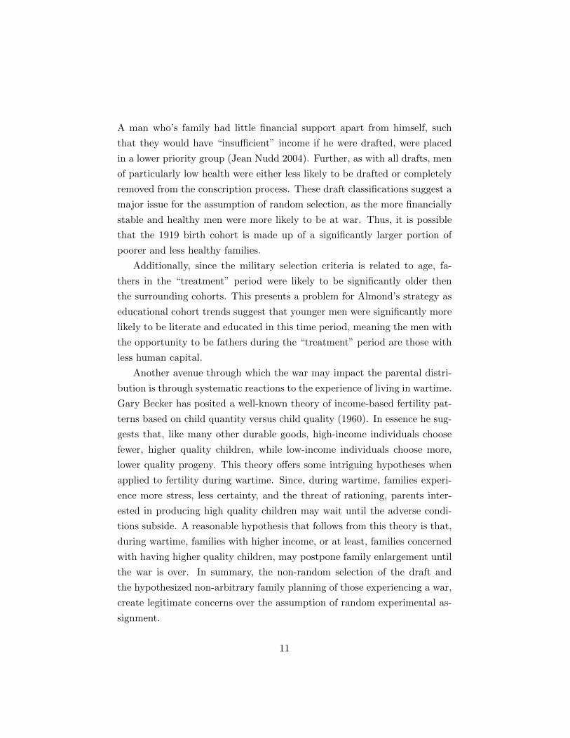
future of one’s child. In fact, graphs such as Figure 2, from Almond’s 2006

paper, have become common starting points for policy makers and scientists

who would like to stress the importance of fetal programming. As mentioned

in the introduction though, results from natural experiments rest precari-

ously on the assumption of randomness. Thus, it is critical to investigate

the theoretical foundation on which this natural experiment is built, because

while there is no denying the stark clarity of Figure 2, the interpretation of

the diagram becomes quite different if exposure status is non-random in a

manner correlated with poor later life outcomes.

Figure 3 plots the average socioeconomic status in 1930, as measured

by Otis Duncan’s socioeconomic index (SEI), of the fathers of people born

between 1912 and 1922 by year of birth from the 1930 U.S. Census.6 This

figure, as Duncan Thomas established, strongly suggests that the 1919 birth

cohort, the cohort of interest in Almond’s work, had fathers of substan-

tially lower socioeconomic quality. This stylized fact does not fit the general

5In his paper, Almond provides tables for women and non-whites with similar results.6Figure 3 is a replication of a graph created by and first shown to the researcher by

Prof. Duncan Thomas (2010).

9

history given by Douglas Almond and greatly hinders the assumption of

randomness necessary for his natural experiment. In the next section this

paper will highlight a major event in U.S. history that was taking place dur-

ing the pertinent period and describe how the impact of this event may help

to clarify the cause of the non-random selection that Figure 3 suggests.

III The Great War and its Implications

The major threat to Almond’s natural experiment framework is the fact

that overlapping the 1918 U.S. influenza pandemic was an event that signifi-

cantly impacted fertility during the entire “treatment” period; World War I.

Not only is a war of its magnitude always of great demographic significance

when evaluating a particular time period, but, in addition, the timing of the

United States involvement in WWI is directly correlated with the creation

and spread of the 1918 influenza bug.

The United States declared war on Germany in April 1917, was regu-

larly sending troops in the summer of 1918, and had accepted Germany’s

surrender by November 1918. Thus, during the key conception periods of

Almond’s studies, the second and third quarter of 1918, a large and select

group of child bearing age men were either stationed in an army barracks

or overseas. In other words, the “treatment” cohort is made up of children

whose fathers are predominately less likely to have served in WWI. For this

selection issue to be a problem, that is create upward and thus misleading

bias of the importance of fetal heath, it would have to be the case that WWI

veterans were, on average and significantly, men of higher parental quality.

While in many wars this would not seem like a reasonable fear, there are

some legitimate reasons for concern in this case.

First of all this was the first war in which a U.S. citizen was not allowed

to hire a proxy to serve in his place. This ruled out the possibility of the

upper class simply buying their way out of service. In fact, due to the

draft categories in use in 1917, men with means were more likely to be

conscripted. While almost all draft eligible men were put in Class I, one of

the main deferments was based on the income dependency of one’s family.

10

A man who’s family had little financial support apart from himself, such

that they would have “insufficient” income if he were drafted, were placed

in a lower priority group (Jean Nudd 2004). Further, as with all drafts, men

of particularly low health were either less likely to be drafted or completely

removed from the conscription process. These draft classifications suggest a

major issue for the assumption of random selection, as the more financially

stable and healthy men were more likely to be at war. Thus, it is possible

that the 1919 birth cohort is made up of a significantly larger portion of

poorer and less healthy families.

Additionally, since the military selection criteria is related to age, fa-

thers in the “treatment” period were likely to be significantly older then

the surrounding cohorts. This presents a problem for Almond’s strategy as

educational cohort trends suggest that younger men were significantly more

likely to be literate and educated in this time period, meaning the men with

the opportunity to be fathers during the “treatment” period are those with

less human capital.

Another avenue through which the war may impact the parental distri-

bution is through systematic reactions to the experience of living in wartime.

Gary Becker has posited a well-known theory of income-based fertility pat-

terns based on child quantity versus child quality (1960). In essence he sug-

gests that, like many other durable goods, high-income individuals choose

fewer, higher quality children, while low-income individuals choose more,

lower quality progeny. This theory offers some intriguing hypotheses when

applied to fertility during wartime. Since, during wartime, families experi-

ence more stress, less certainty, and the threat of rationing, parents inter-

ested in producing high quality children may wait until the adverse condi-

tions subside. A reasonable hypothesis that follows from this theory is that,

during wartime, families with higher income, or at least, families concerned

with having higher quality children, may postpone family enlargement until

the war is over. In summary, the non-random selection of the draft and

the hypothesized non-arbitrary family planning of those experiencing a war,

create legitimate concerns over the assumption of random experimental as-

signment.

11

These hypotheses suggest that the income, health, and education of the

parents of the 1919 birth cohort were significantly lower than surrounding

birth cohorts. This type of sorting would present a major problem for iden-

tifying the impact of maternal health on the child’s later life wealth, health,

and education conditions, as numerous studies have connected parental

wealth, health, and schooling with these very same outcomes (Davis-Kean

2005, Duflo 2000, Thomas and Strauss 1998, Brooks-Gunn and Duncan

1997, Corcoran et al. 1992, Hill and Duncan 1987). Additionally, if fam-

ilies interested in raising quality children were more likely to select out of

the 1919 birth cohort, as is suggested by the Becker hypothesis, this would

obviously cause being in the “treatment” group to misidentify the impact

of fetal health on the outcomes of interest.

While Figure 3 suggests that the concerns presented in this section are

real, the goal of the remainder of this paper is to rigorously compare the fam-

ily characteristics of those born in 1919 with the surrounding birth cohorts.

Namely, this paper will test the hypotheses that assert that the parents of

children born in 1919 were significantly worse in the areas of income and

education, that they were older, and that they desired a larger quantity,

rather than a higher quality of children, than the parents of children from

surrounding cohorts.7 The next three sections will present three approaches

to analyzing the validity of these suppositions.

IV First Approach, 1930 U.S. Census Data

IV.1 Methodology

To examine the hypotheses, it was imperative to find data that contained

the parental characteristics of the early 1900’s birth cohorts. As Almond,

this research takes advantage of the comprehensive and demographically rich

U.S. Census data. The IPUMS 1% sample of the 1930 U.S. Census data is

particularly useful as it contains information on the parents of U.S. born

7Unfortunately, this paper is unable to directly test the hypothesis that the 1919 birthcohort had significantly less healthy parents as no variable that measured or could proxyfor parental health existed in the data.

12

children over the entire time period of Almond’s 2006 analysis, 1912 - 1922.

Although the range of parental characteristics is not exhaustive in relation

to this study’s hypotheses, the 1930 census contains ample demographic

statistics to provide informative analysis.8

One area in which the 1930 census is particularly thorough is in infor-

mation about the economic status of the parents, which includes outcomes

such as whether the father is in the labor force, the father’s Duncan’s SEI

score, the father’s occupational income score, and the father’s occupational

earnings score.9 An additional proxy for wealth is whether the family owns

a radio, as radio ownership is a clear sign of disposable income. A less rich

data category is education. Unfortunately, the only relevant educational

characteristic, other than what is inherent in the Duncan’s SEI score, is the

parent’s literacy. More promisingly, family size can be used to address the

quantity versus quality hypothesis. In this case, the number of the father’s

or mother’s children in the household will be used as a signal of a family’s

preference. Another nice element of the 1930 census data is that it can be

used to directly test the inference that children born in 1919 were less likely

to be the child of a WWI veteran. Finally, the age of the parents at the

time of the child’s birth will be used to test if the 1919 birth cohort had

significantly older parents than those in surrounding cohorts. This data,

with all its richness, is not without its drawbacks.

The 1930 U.S. Census was collected on April 1, 1930 and, rather than

asking for the birth date information of the respondents, they simply asked

for their age as of March 31, 1930. Due to this data collection decision,

this approach is limited to placing people into birth cohort bins between

April 1st and March 31st rather than January 1st and December 31st. This

hinders the analysis, in that, the birth cohort of interest, 1919, loses a major

8All data is as of March 31, 1930.9Otis Duncan’s SEI is a measure of occupational status based upon the income level

and educational attainment associated with each occupation in 1950. Occupational incomescore assigns each occupation a value representing the median total income (in hundreds of1950 dollars) of all persons with that particular occupation in 1950. Occupational earningsscore is created in two steps. First a z-score indicating the number of standard deviationsby which each occupational category differed from the mean earnings of all occupationsis created. Then these scores are translated into a percentile rank.

13

quarter of exposure, those conceived in the 2nd quarter of 1918, and replaces

them with an unexposed group, those conceived in the 2nd quarter of 1919.

Theoretically, this would simply cause the results to be a lower bound, but

due to the lack of more precise birth date data, this problem cannot be

solved directly. In the rest of Section IV, unless otherwise noted, reference

to any birth year indicates the person was born between April 1st of that

year and March 31st of the subsequent year.

As this study purposefully follows Almond’s own model, the 1919 birth

cohort will be isolated to test if it is significantly different than the surround-

ing cohorts, 1912 to 1922, while controlling for the time trend.10 The only

difference in the two models is that where his outcomes, yi, were individual

i’s outcomes in later years, the dependent variables in these specifications

are the individual’s parent’s characteristics in 1930:

yi = β0 + β1 · Y OBi + β2 · Y OB2i + β3 · Ii(Y OB = 1919) + εi (2)

Since the specification choice was made to mirror Almond’s work this

study’s main findings use a model that includes a quadratic in the time trend.

It should be noted, though, that at no time in Almond’s 2006 study does he

provide the basis for his decision to include a quadratic in the time trend,

and further, no obvious historical or theoretical intuition for its inclusion is

apparent. Thus, all the results presented in this section are accompanied

in the Appendix by identical analysis that excludes this variable, Tables

A1 - A3. The change does not substantially impact any of the results or

interpretations.

IV.2 Results

Table 4 presents the coefficient estimates of β3 from the analysis of the

IPUMS 1% sample of the 1930 U.S. Census. The education coefficients,

while not significant, each have the predicted sign. Further, the indicators

of economic success are almost all significantly negative, at least at the

10The actual period used in the analysis was April 1st, 1911 to March 31st, 1923, inorder to capture all the respondents born between 1912 and 1922.

14

10% level. This suggests that there was some treatment group assignment

bias with respect to an individual’s wealth. In regards to one of the other

hypotheses, it is clear that the 1919 birth cohort is a member of significantly

larger families, suggesting that Becker’s theory of quality versus quantity

may be biasing Almond’s findings. Additionally, a further marker of parental

composition, age of parent at birth, suggests that the parents of the 1919

birth cohort were significantly older at the time of the child’s birth. Aside

from the negative distributional change this suggests with respect to the

education of the parents of the 1919 birth cohort, this fact can also adversely

impact a child’s long-term educational, economic, and health outcomes in a

few additional ways.

First and foremost, children of older mothers have more health prob-

lems/risks than those of younger mothers, including birth defects, low birth

weight, Down syndrome, and autism (Park and Falco 2010). In fact, it has

even been shown that the age of the father is positively correlated with

autism incidence in their children. Beyond the severe initial health risks

they pose, older parents also need care from their children at a younger age

which is associated with significantly higher levels of stress (Deimling and

Bass 1986; Noelker and Townsend 1987; Stoller and Pugliesi 1989). Further,

this additional need for care earlier in the child’s life may stunt their edu-

cational and income trajectories, as the time, effort, and money spent on

caring for the aging parent can limit the child’s ability to take advantage of

all opportunities and fully realize their potential.

Finally, the results using two additional parental characteristics are worth

noting. First, as expected, the 1919 birth cohort is significantly less likely

to be the child of a World War I veteran. Furthermore, a child born in the

U.S. in 1919 was significantly less likely to have Caucasian parents. The

latter of these composition differences is a clear signal of being born into a

less ideal environment as, in 1930 America, being white provided not just

circumstantially better educated and more economically viable parents but,

due to rampant racism, also better long term opportunities for one’s own

achievement. Moreover, as mentioned, the draft classifications would suggest

that children of non-WWI veterans are more likely to be born into finan-

15

cially unstable households. To more firmly establish both of these claims,

this study examined the correlation between being a white father or being a

WWI veteran father and the father’s literacy, economic standing, and num-

ber of children while controlling for the father’s age, father’s age squared,

and state of birth fixed effects. For each variable, being white or being a

WWI veteran was significantly positively related to having more desirable

traits.11

The 1930 U.S. Census indicates that the parents of the 1919 birth co-

hort were not random. Further, the attributes on which they selected into

the “treatment” group are all negatively related to the child’s future edu-

cational, economic, and health outcomes. While these results suggest that

identification issues exist for Almond’s findings, to feel entirely confident, it

is important to make sure that the underlying census data is not biased and

that the findings are unique to the 1919 birth cohort.

IV.3 Tests of Robustness

There are two main areas of sampling concern with respect to using the

1930 U.S. Census data. First, it is a reasonable conjecture that fathers of

the 1919 birth cohort were less likely to be in WWI. Further, to be included

in the regressions related to a father’s characteristics, one’s father must be

alive in 1930. If it were the case that smarter and more economically viable

soldiers were less likely to be killed at war, then the sample of pre-war birth

cohort fathers may be biased because the weakest fathers are missing. If this

issue is a valid concern, it should be the case that the children born before

the war are significantly more likely to be missing data on their fathers.

Evidence of this problem is not found.12 Thus, while the intuition presents

a problem, the data does not identify this bias.

A second area of concern is that the 1930 U.S. Census does not contain

data for one’s parents if the person was living independently from their par-

ents. This is particularly problematic if those children that move out and

live by themselves earlier are the children from lower quality households. To

11The results of this analysis can be found in the Appendix, Table A4.12Analysis provided upon request.

16

determine the severity of this problem this study examined if early birth co-

horts, the older children in 1930, had significantly less parental information.

In the end, only the earliest birth cohort in the trend, 1912, exhibited this

problem. Another way this issue could come into play is if the women from

the most low quality households are being married off significantly younger

than others. After a close examination of the data, it does appear that

women in the pertinent period, 1912 to 1922, are significantly more likely to

be missing parental than men. To test the robustness of the results to each

of these potential composition concerns, the regressions from Table 4 were

separately run using one specification that only included the period 1913 to

1922 and another which only used data on male children.

Table 5 presents the estimates when using the smaller time period. The

results are very consistent with the base case in Table 4. Similarly, in Table

6, where only male children are included, only 2 of the 10 original significant

findings have lost statistical significance. In addition, the point estimates

from most of the remaining statistically significant regressions, owning a

radio, father’s occupation score, family size, and race, have all increased.

An additional potential critique of the findings in Table 4 is that, due to

the large sample size being used, they may be non-unique to the 1919 birth

cohort. If similar estimates, in sign and significance, are found for other

birth cohorts the interpretation and importance of the results of Table 4

would be greatly hindered. Thus, to add strength to the results, placebo

tests were run in which the dummy variable for the 1919 birth cohort was

replaced by either an indicator variable for the 1917 birth cohort or the 1920

birth cohort.13,14 Using either specification, estimates are non-significant or

opposing from those in Table 4 in the literacy, socioeconomic status, family

size, and parental age estimates. Only 2 of the 32 placebo regressions provide

significant results in the same direction as Table 4, lending support to the

13To be a true placebo test the 1917 birth cohort was used rather than the 1918 birthcohort because the approximation of the 1918 birth cohort in the 1930 U.S. Census datacontains an important quarter of the exposure group, those born in the first quarter of1919.

14The results of this analysis can be found in the Appendix, Tables A5 and A6, respec-tively.

17

uniqueness of the 1919 birth cohort estimates.

In summary, even after testing for robustness, the overall message re-

mains consistent; the children born in 1919 had family situations that were

significantly more undesirable than children from the surrounding cohorts.

Additionally, these results were significant despite losing a key segment of

the pertinent birth cohort due to the limitations of the 1930 U.S. Census

data. Including the children of the 1919 birth cohort that were unable to

be properly assigned, those conceived in the 2nd quarter of 1918, should

only strengthen the results. To address this inadequacy, as well as, to take

a closer look at the timing of the treatment assignment bias, a second ap-

proach which uses the 1920 U.S. Census data was employed.

V Second Approach, 1920 U.S. Census Data

V.1 Methodology

Using the 1920 U.S. Census data provides some straightforward gains.

First and most importantly, the 1920 census was taken on January 1st,

1920, thus one’s age accurately predicts the respondent’s year of birth and

each birth cohort can be accurately identified. Further, in this census they

recorded the age in months of all children 5 years old and younger, which

means that for the birth cohorts from 1915 to 1919 the researcher knows the

child’s conception date down to the month. By exploiting these advantages,

the study can examine the parental attributes of the true 1919 birth cohort,

as well as, speak directly to the fact that children conceived in the 2nd and

3rd quarters of 1918 drive Almond’s findings. Additionally, due to the fact

that the cohorts of interest are 10 years younger in 1920, there is no concern

that lower quality older children will have moved out, and as such, left the

sample.15 Along with these beneficial elements of the 1920 census data,

though, are some obvious shortcomings.

The major problem with using data obtained on January 1st, 1920 is

15As before, the father’s data is not missing significantly more for the pre-war cohorts.

18

that the comparison group loses almost the entire post pandemic cohort.16

Although all indications from the 1930 U.S. Census analysis suggest that

this is not the case, losing the post pandemic cohort leaves the significant

differences found in the 1919 birth group open to the interpretation that they

are simply the result of the start of a new trend. An additional restriction

for this data, as mentioned above, is that the 1920 U.S. Census only has

the more detailed age data back to 1915. Thus, analysis that wishes to use

month or quarter of birth information is even more constrained. Finally,

in the 1920 U.S. Census they do not ask about military status or radio

ownership, so both of these outcomes are no longer testable.

The primary specification will be the same as equation (2) except the

indicator for being born in 1919 will actually refer to being born between

January 1st 1919 and December 31st 1919 and the trend will be from 1912

to 1919. A second model is used to establish the timing of the 1919 differ-

ences. Related in spirit to a similar regression in Almond 2005 it splits the

1919 birth year indicator into four separate quarter-of-1919 birth dummy

variables. In addition, this model includes dummy variables for quarter of

birth to control for the types of seasonal effects on the education and income

composition of families that choose to have children during these quarters

(Buckles and Hungerman 2008). As before, all the regressions were addi-

tionally run excluding the year of birth quadratic term. The alternative

estimates were consistent with the main results and can be found in the

Appendix, Tables B1 and B2.

V.2 Results

Table 7 presents the coefficient estimates of the 1919 birth cohort dummy

from regressions over the 1912 to 1919 time period. The majority of the

results are identical in interpretation to the estimates using the 1930 U.S.

Census data. One conclusion for which there is a change is that being

born in 1919 now has no significant relationship with the probability of

one’s father being in the labor force. This non-result, though, may stem

16Only the 4th quarter 1919 birth cohort could be considered relatively unexposed.

19

from the fact that so few fathers are not in the labor force in 1920, only

1.2%. If the 1919 birth cohort fathers were just as likely to be employed

in 1920 as the fathers of the previous cohorts, it is hypothesized that they

were employed in significantly lower income jobs. The results confirm this

expectation. For both occupation score variables as well as the Duncan SEI

outcome, fathers of children born in 1919 are doing significantly worse in

1920, after controlling for the time trend, than the fathers of the previous

cohorts. Additionally, unlike in the previous section, both of the study’s

education proxies are now significant. Further, as before, the 1919 birth

cohort is part of significantly larger families, has significantly older parents,

and is significantly less likely to have white parents. Once again, the findings

suggest that “treatment” group assignment is non-random in a way that is

correlated with potential for poor later life outcomes.17 What must still be

addressed are Almond’s findings that the 1st and 2nd quarter 1919 births

have the poorest long-term outcomes. Table 8 presents results that explain

these results through selection bias.

Table 8 displays the coefficient estimates for each of the quarter dummy

variables of the 1919 birth cohort when using data from the 1915 to 1919

time period. The results mirror those in Table 7 and also offer a counter to

Almond’s claim that there should be no concern over non-random selection

into giving birth during the 1st two quarters of 1919. In stark contrast, both

of these quarters portend significant sorting behavior based on education,

income, family size, parent’s age, and race. Further, since the direction of all

the coefficients indicate poorer conditions and they are usually the largest of

the point estimates, it is unsurprising that Almond finds the worst outcomes

for these cohorts.

Finally, as a counterpoint to Almond’s Figure 1, Figure 4 presents the

point estimates from each quarter of birth dummy over the 1916 to 3rd

quarter 1919 time period from a regression of father’s literacy rate, which

17As before, a placebo test was used to determine the uniqueness of the results. Theestimates from regressions which replaced the 1919 birth cohort dummy with an indicatorvariable for the 1918 birth cohort are found in the Appendix, Table B3. In support ofthis study’s hypotheses, none of the results were similar in sign and significance to thosein Table 7.

20

controls for a birth year trend and seasonal effects (estimated over the 1915

to 1919 birth cohorts). As is clear, being born in the first 3 quarters of

1919 has an adverse relationship with father’s literacy, severely hindering

the inference Almond makes when presenting Figure 1. As in Section IV,

the sum of the results indicates an acute problem for Almond’s ability to

determine the impact of fetal health on long-term health, wealth, and edu-

cational outcomes. As mentioned earlier though, this dataset, due to its lack

of post-pandemic cohorts, may not hold water for all skeptics, so an attempt

was made to repeat the analysis using a dataset which pulls together the

benefits of both the 1920 and 1930 U.S. Censuses.

VI Third Approach, Combining Datasets

VI.1 Methodology

The previous section shows the power one gains in this analysis by cor-

rectly specifying the 1919 birth cohort. In particular, the quarter that the

1930 census analysis loses, the 1st quarter of 1919, is especially important

to the results. It seems reasonable that if the 1919 birth cohort could be

accurately determine in the 1930 census data, the results in section IV would

make an even stronger statement. The final approach used in this study adds

the 1920 U.S. Census’s ability to correctly identify the 1919 birth cohort to

the more complete 1930 U.S. Census data.

The first hurdle when combing these two datasets is that, as mentioned

previously, they were conducted during different parts of the year and do not

contain complete birth date information. This makes defining a consistent

“birth year” variable more difficult. In order to do this, the part of the 1920

census data that also provides quarter of birth data is used, so that, as is

the case in the 1930 U.S. Census, birth year can be defined as of March 31st.

The combined dataset uses 1930 census information for the periods April

1st, 1911 to March 31st, 1915 and April 1st, 1920 to March 31st, 1923 and

1920 census information for the period April 1st, 1915 to December 31st,

1919. Constructed in this way, the dataset can accurately identify all the

21

members of the 1919 birth cohort and contains the post-pandemic cohorts

of interest. The drawback is that, by combining the censuses, one loses the

entire January 1st, 1920 to March 31st, 1920 birth cohort.

While losing this data is far from ideal, analysis of the children born from

1915 to 1919 indicate that families who have their child in the first quarter

of the year, controlling for those born in the 1st quarter of 1919, are sig-

nificantly more literate, economically viable, and more likely to be white.18

Following this logic, losing the 1st quarter 1920 birth cohort simply causes

the analysis to underestimate the low quality of the parents of the 1919 birth

cohort. The only variable for which there is concern that excluding the 1st

quarter of 1920 birth cohort would overestimate the results is with age at

birth, as the parents of first quarter children are significantly older during

the 1915 to 1919 period, even when controlling for the first quarter 1919

birth cohort.

Choice of specification, when using the combined dataset, is also a bit

more complicated. First of all, due to the fact that these responses are taken

from separate censuses, given 10 years apart, there are certainly temporal

and life cycle shifts in education and economic standing that need to be

controlled. Further, beyond a simple intercept shift, there also may have

been a change in the slope of outcomes. In this analysis, though, the slope

change seems less likely as it would have to be assumed that, in the 10 years

since 1920, the change in outcomes between parents, assumed to be on

average one year different from each other, has significantly shifted trends.

The initial choice of specification was a model consistent with the previ-

ous analysis, which simply added a dummy variable for the 1930 census.19

This model is slightly flawed though, as it does not account for the fact that,

unlike in the previous analysis, birth year no longer linearly predicts the age

of the child at the time of survey. For example in this combined data a

child born in 1914 is 16 at the time of survey, 1930, while a child born in

18Father’s inclusion in the labor force, as well as, the family size variables were notsignificantly different than zero.

19Estimates from this model are completely consistent with the primary model used inthis section except for in the regressions on family size. Analysis provided upon request.

22

1915 is 5 at the time of survey, 1920. To control for this, following Almond

2005, an alternate specification choice is used that includes the 1930 survey

year dummy, as well as, a quadratic in age of survey interacted with the

1930 census dummy term. Also, similar to Almond 2005, multiple other

specifications were estimated with consistent results.20 As in the previous

sections, estimates from the main model, which exclude the year of birth

quadratic, are completely consistent with the primary results and are found

in the Appendix, Tables C1 - C3.

VI.2 Results

The coefficient estimates of the 1919 birth year dummy variable using

the combined dataset are presented in Table 9. Consistent with all the

previous findings, the 1919 birth cohort has fathers who are significantly less

occupationally prosperous, have significantly lower socioeconomic status,

and come from larger families with older parents.21 Additionally, as was the

case using the 1920 census, the estimates from the combined data indicate

that the parents of the 1919 birth cohort are significantly less literate. Taken

together, these findings continue to confirm the suspicion that Almond’s

natural experiment is non-random in a way which clouds identification of

the impact of fetal health on long-term outcomes.

VI.3 Tests of Robustness

The same attrition concerns espoused in Section IV are present in the

combined dataset. As before, the concern over losing pre-war cohort data

from relatively lower quality fathers who passed away in the war, is not

empirically founded, as there is no significant relationship between missing

one’s father’s information and being born before WWI. On the other hand,

as in Section IV, there does appear to be a relationship between missing

parental data and being from the 1912 birth cohort or being an older girl.

20Estimates of three alternate models can be found in the Appendix, Tables C4 - C6.21As mentioned previously, the age of the parents’ estimates may be biased due to the

missing 1st quarter 1920 birth cohort.

23

As in Section IV, robustness tests were conducted by repeating the analysis

from Table 9 using one specification that only included the period 1913

to 1922 and another that only used data on males. The results for these

two analyses can be found in Tables 10 and 11, respectively. The inference

made on the estimates from these alternative models remains completely

consistent with the primary findings.

Finally, as in the previous sections, placebo tests were conducted to

examine the uniqueness of the findings with respect to the 1919 birth cohort.

Tables C7 and C8, in the Appendix, provide the results of regressions which

replace the 1919 birth cohort indicator variable with dummy variables for the

1918 birth cohort and the 1920 birth cohort, respectively.22 In congruence

with the previous placebo tests, Tables C7 and C8 support this study’s

hypotheses, as none of the estimates are similar in sign and significance to

the main findings found in Table 9.

VII Discussion

The previous three sections make a strong case that the parents of the

1919 birth cohort were significantly different than the parents of surrounding

cohorts in areas that damage the identification strategy used in Almond’s

U.S. influenza papers. The next appropriate step to take, after identifying

this bias, is to estimate to what extent controlling for parental character-

istics reduces the magnitude and significance of Almond’s findings. Unfor-

tunately, testing this directly is not possible as neither data source used

in Almond’s U.S. influenza papers (U.S. Census and SIPP) has data on

parental or family background characteristics. In order to provide a lower

bound approximation of the importance of factoring in parental characteris-

tics when examining the persistent effect of fetal health using the 1918 U.S.

influenza pandemic, an additional analysis was conducted.

The strategy was to replicate Douglas Almond’s 2006 work, which uses

22Due to the appending process and the 1930 U.S. Census data, the 1920 birth cohortdummy used in these regressions represents people born between April 1, 1920 and March31, 1921.

24

the 1960, 1970, and 1980 IPUMS samples, and compare his findings to the

same model which additionally includes as close a control for parental char-

acteristics as is available in the data.23 The most useful data to proxy

parental characteristics is information about the respondent’s childhood en-

vironment. The only variables that fit this description in the data are the

respondent’s state of birth and race. While these variables are clearly insuffi-

cient to hold constant all the differences in parental characteristics identified

in the previous sections, incorporating them into the regressions can serve

as a partial control for the differential childhood environment factors faced

by the 1919 birth cohort.24

This correction analysis was conducted by first replicating Almond’s 2006

findings using his original specification (shown in Equation 1) and then

comparing the magnitude and significance of the point estimates on the 1919

birth cohort dummy variable to the same model that additionally includes

23The data used for the replication and additional analysis was the same IPUMS U.S.Census microdata used in Almond’s work, except, while he did not use any age or birth-place data with a census quality flag above 3, this study does not use any variable’s valuewhich had a quality flag above 3. In addition, this study’s analysis removed any individ-ual not born in the U.S. These changes in the data had little impact on the magnitudeor significance of his original findings. In the 54 regressions replicating Almond’s work,the significance level interpretation (significant at or below 5%, vs. other) only changed6 times. Further, of these 6 changes, two resulted in lower p-values, three only changedfrom significant at or below the 5% level to having p-values between .06 and .09, and onlyone changed from significant at the 5% level to insignificant.

24Along with the methodology already mentioned, in his 2006 paper, Douglas Almonduses an alternative strategy in order to look at outcome differences by state of birth. Inthis analysis he uses maternal mortality rates by state and year prior to birth to proxyfor infection intensity. This methodology though, does not control for the identificationbiases discussed in this paper, as high maternal mortality rates in one year are likely to becorrelated with poor parental characteristics and a weaker health environment for the nextbirth cohort. High maternal mortality rates, particularly when the rate is trending up, canserve as a signal of a poor quality health environment. In states where maternal mortalityrates where relatively high or steadily increasing in the previous year, the families that stillchoose to conceive a child are likely to have weaker preferences for health and the childis likely being born into an increasingly low quality health environment. Using Almond’sstate of birth model the subsequent inferior long-term outcomes of the child would simplybe viewed as the result of poorer in utero health, and the findings would seemingly verifyAlmond’s hypotheses. As is apparent from this example though, the fetal health variationAlmond is using in this analysis is significantly correlated with parental and environmentalcharacteristics and, similar to his simpler methodology, a failure to control for these factorswill lead to biased results.

25

indicators for the respondent’s state of birth, race, and an interaction of

the two.25 By using this alternative model the comparison group that the

members of the 1919 birth cohort is being evaluated against will be stripped

of the differential parental characteristics that are constant within a state,

racial group, and its interaction over this time period.

Tables 12 and 13 present the results of this analysis for men and women,

respectively. As an overview, of the 37 estimates of the 1919 birth cohort

effect that had the sign that corresponded to Almond’s hypothesis and were

significant at or below the 5% level in the 2006 paper, approximately 40%,

14, are no longer significant at that level.26 Further, on average, those 37

point estimates lost 40% of their magnitude.

The results that hold up the most to these artificial controls for parental

characteristics are the education regressions. None of the 12 male or female

regressions of interest, which look at high school graduation or total years

of education, lose their significance. Even with no changes of statistical sig-

nificance though, the magnitudes of the point estimates are greatly reduced.

The high school graduation point estimates are reduced by an average of

one-third (34% for men and 32% for women) and the years of education

magnitudes are reduced by 42% (40% for men and 44% for women). These

findings suggest that at least at an upper bound, Almond’s estimates, while

greatly reduced, still remain significant for educational outcomes. The esti-

mates using the financial outcomes are less favorable.

Of the 18 regressions of interest that deal with in utero health’s impact

on long term financial outcomes (total income, wage income, neighbors’ in-

come, poverty, and Duncan’s SEI) half of the results are no longer significant

25The race variable used is an indicator variable taking the value one if the subject iswhite and zero otherwise. All regressions follow Equation 1, except in the few instancesthat Almond specifically uses a different model. The “years of disability in 1970” regres-sions were not replicated as the public data only had it coded as a categorical rather thanordinal variable.

26This 37 drops two regressions that fit the criteria given in the text; the 1970 regressionfor men on “years of disability” as it was not replicated for reasons mentioned in footnote25, as well as, the 1970 regression for women on “disability prevents work”, as simplyusing higher quality data, even before fixed effects were introduced, made the coefficientnon-significant.

26

at the 5% level. As expected the magnitudes are also greatly reduced; the

point estimates of interest are reduced by approximately 44% for men and

51% for women (56% for the 9 made non-significant and 37% for the 9 that

remained significant at the 5% level). Taken all together, these results sug-

gest that, even at an upper bound, Almond’s findings with regard to in

utero health’s impact on later life economic well-being is greatly diminished

once parental characteristics are controlled. Similarly, the effects on disabil-

ity and entitlement payments are also not supportive of Almond’s original

findings.

To analyze fetal health’s impact on adult health Douglas Almond’s 2006

research uses measures of disability and entitlement payments as its indi-

cators. For males, he finds some consistent and significant support for the

hypothesis that the 1919 birth cohort is more likely to have a disability that

prevents or limits work and more likely to be receiving entitlement payments

(6 of his 8 estimates are significant at the 5% level), but when the same re-

gressions are run adding proxies for parental characteristics, the evidence is

greatly attenuated. Four of the 6 previously significant results are no longer

significant at the 5% level, and the point estimates are reduced by an aver-

age of 25% after partially controlling for childhood environment. Further,

when analyzing women, Almond’s results were mostly non-supportive; only

2 of 8 were originally significant at the 5% level and had the hypothesized

sign and, moreover, 1 of the regressions was significant and had the oppo-

site sign. Additionally, when the regressions were re-estimated, one of these

two supportive findings lost significance once the controls were added, and

the other’s significance was unable to be replicated with either the original

or alternative specification as mentioned in footnote 26. In summary, of

the 16 estimates of the impact of in utero health on disability and entitle-

ment payments, only 2 remained significant at the 5% level with Almond’s

hypothesized sign once proxies for parental characterizes were added.

While the two analysis described in this section is imperfect, it makes

a point consistent with the previous sections; the sample selection issue

expressed in this study has a significant attenuating effect on the magnitude

and power of results that use the 1918 U.S. influenza pandemic as a natural

27

experiment for in utero health and do not control for parental characteristics.

VIII Conclusion

Testing the fetal-origins hypothesis using methods other than a natural

experiment is rife with empirical and logistical issues. Controlling for all the

unobserved parental characteristics correlated with both a parent’s health

and a child’s later life outcomes, as well as, obtaining data which includes

the health of pregnant mothers, family characteristics, and follows the child

to adulthood is seemingly impossible. Further, experimenting with mater-

nal health has ethical constraints, as well as, financial burdens inherent in

tracking the sample children for several decades. Given this reality, a num-

ber of researchers, as documented in Section II, have tried to use the natural

experiment framework with limited precision and varying results. Douglas

Almond’s clever use of the 1918 U.S. influenza pandemic and its landmark

findings appeared to be the long awaited breakthrough in the study of fetal

health’s persistence. What was taken for granted though, was the appropri-

ateness of the natural experiment framework to the U.S. experience of the

influenza pandemic. This paper set out to explore the underlying assump-

tions necessary to support Almond’s influential findings.

The more complete historical circumstances, presented in Section III, led

to reasonable hypotheses that challenged the concept of randomness neces-

sary to the use of the 1918 U.S. influenza pandemic as a natural experiment.

The approaches presented in Sections IV-VI, while each having their own

unique data limitations, consistently confirmed many of these suppositions,

including that families of the “treatment” group were significantly less edu-

cated, less wealthy, and larger. Most damaging to Almond’s inference, each

of these characteristics is a direct or theoretical sign of low quality parentage

that can impact a child’s later life health, wealth, and educational outcomes.

While this paper in no way comments on the legitimacy of the fetal-origins

hypothesis, it does assert that its most seminal work in economics has large

enough identification ambiguity to make its estimates untenable.

28

IX References

Almond, D. (2006). “Is the 1918 Influenza Pandemic Over? Long-Term

Effects of In Utero Influenza Exposure in the Post-1940 U.S. Population.”

Journal of Political Economy, 114 (4), 672-712.

Almond, D. and Mazumder B. (2005). “The 1918 Influenza Pandemic

and Subsequent Health Outcomes: An Analysis of SIPP Data.” American

Economic Review Papers and Proceedings, 95 (2), 258-62.

Barker, D. (1994). Mothers, Babies, and Disease in Later Life, London:

BMJ Publishing Group.

Becker, G. (1960). “An Economic Analysis of Fertility.” in:Demographic

and Economic Change in Developed Countries, Princeton: Princeton Uni-

versity Press for the National Bureau of Economic Research.

Brainerd, E. and Siegler M. (2003). “The Economic Effects of the 1918

Influenza Epidemic.” Discussion Paper no. 3791, Centre Econ. Policy Res.,

Paris. British Medical Journal , July, 13 1918.

Brooks-Gunn, J. and Duncan G. (1997). “The Effects of Poverty on

Children.” The Future of Children, 7 (2), 55-71.

Buckles, K. and Hungerman D. (2008). “Season of Birth and Later

Outcomes: Old Questions, New Answers.” Working Paper No. 14573 (De-

cember), NBER, Cambridge, MA.

Corcoran, M., Gordon, R., Laren, D., and Solon, G. (1992). “The Asso-

ciation Between Men’s Economic Status and Their Family and Community

Origins”.J. Hum. Resour. 27, 575 601.

Crawford, Richard. (1995). “The Spanish Flu,” Stranger Than Fiction:

Vignettes of San Diego History., San Diego Historical Society.

http://edweb.sdsu.edu/sdhs/stranger/flu.htm

Davis-Kean, P. (2005). “The Inuence of Parent Education and Family

Income on Child Achievement: The Indirect Role of Parental Expectations

and the Home Environment.” Journal of Family Psychology, 19 (2), 294

-304.

Deimling G. and Bass, D. (1986). “Symptoms of Mental Impairment

Among Elderly Adults and their Effects on Family Caregivers.” Journal of

29

Gerontology: Social Sciences, 41, 778-785.

Duflo, E. (2000). “Child Health and Household Resources in South

Africa: Evidence from the Old Age Pension Program.” American Economic

Review Papers and Proceedings, 90 (2), 393-98.

Hill, M.. and Duncan, G. (1987). “Parental Family Income and the

Socioeconomic Attainment of Children.” Soc. Sci. Res., 16, 37 73.

Kannisto, V. , Christensen K., and Vaupel J. (1997.) “No Increased

Mortality in Later Life for Cohorts Born during Famine.” American J. Epi-

demiology, 145 ( June 1), 98794.

Neugebauer, R., Hoek H., and Susser, E..(1999). “Prenatal Exposure

to Wartime Famine and Development of Antisocial Personality Disorder in

Early Adulthood.” J. American Medical Assoc., 282 (August 4), 45562.

Noelker, L. and Townsend. A. (1987). “Perceived Caregiving Effec-

tiveness: The Impact of Parental Impairment, Community Resources, and

Caregiver Characteristics.” T. H. Brubaker (Ed.) Aging, Health, and Fam-

ily: Long-Term Care Newbury Park, CA: Sage, 58-79.

Nudd, Jean. (2004). “U.S. World War I Draft Registrations.” Yester-

days, 24 (1), 34-41.

Park, M. and Falco, M. “Older Mothers’ Kids Have Higher Autism Risk,

Study Finds.” CNN.com, Feb. 8, 2010.

http://www.cnn.com/2010/HEALTH/02/08/autism.mother.age.risks/

Rasmussen, K. (2001). “The ‘Fetal Origins’ Hypothesis: Challenges and

Opportunities for Maternal and Child Nutrition.” Ann. Rev. Nutrition 21

(July), 7395.

Ravelli A. et al. (1999). “Obesity at the Age of 50 y in Men and Women

Exposed to Famine Prenatally.” American Journal of Clinical Nutrition, 70,

81116.

Roseboom, T. et al. (1999). “Blood Pressure in Adults After Prenatal

Exposure to Famine.” Journal of Hypertension, 17, 32530.

Roseboom, T. et al. (2000). “Coronary Heart Disease after Prenatal

Exposure to the Dutch Famine, 194445.” Heart, 84 (December 1), 59598.

Stanner, S. et al. (1997). “Does Malnutrition In Utero Determine

Diabetes and Coronary Heart Disease in Adulthood? Results from the

30

Leningrad Seige Study, a Cross Sectional Study.” British Medical Journal,

315 (November 22), 134248.

Stoller, E. and Pugliesi, K. (1989). “Other Roles of Caregivers: Com-

peting Responsibilities or Supportive Resources.” Journal of Gerontology:

SocialSciences, 44, 231-238.

Thomas, D. (2010). “Health and Socioeconomic Status: The Importance

of Causal Pathways.” B. Pelskovic and J.Y. Lin (Eds.) World Bank Annual

Conference on Development Economics.

Thomas, D. and Strauss, J. (1998). “Health, Nutrition, and Economic

Development.” Journal of Economic Literature, 36 (2), 766 817.

www.1918.pandemic.gov

31

X Tables and Figures

32

260 AEA PAPERS AND PROCEEDINGS MAY 2005

250,000-- - 330

200,000-

150,000 . 3 15

?3.o0 3. 10

E o 3 00 1918:1191821918:3 1918:4 19191 19192 19193 19194 z

QuarterlQuarter of Birth Influenza desaths

Average health

FIGURE 2. INFLUENZA DEATHS AND AVERAGE HEALTH INDEX IN SIPP

Individuals born in the third quarter of 1918, just before the height of the Pandemic, have similar levels of reported health as those born in the fourth quarter of 1919, who were conceived after the peak of the Pandemic in October 1918. Most notably, however, we observe a sharp falloff in health for those born during the second quarter of 1919 who were in utero at the height of the Pandemic.

We now present econometric results, which demonstrate the statistical significance of the cohort effects on health. This also allows us to control for the age effects apparent in Figure 1 as well as any survey year effects. Outcomes may change over time due to such factors as technological improvement, changes in medical care access, and attrition of the cohorts. To the extent that these factors may affect certain ages more than others (and thereby potentially bias cohort estimates), it is important to allow the age profile to vary by survey year. Our preferred regression specification therefore controls for survey year dummies and a quadratic in age interacted with survey year.8

In Table 1 we present results where we test for a cohort effect for the entire birth year of

1919 for selected health outcomes.9 For both self-reported health measures, we find that the 1919 cohort effect is large and statistically significant at the 1-percent level. For example, individuals born in 1919 are nearly 4 percentage points more likely to be in fair or poor health (or 10 percent).10 We also find that the 1919 cohort is more likely to have a range of functional limitations, including trouble hearing, speaking, lifting, and walking. These differences are sta- tistically significant and large, resulting in ap- proximately 19-, 35-, 13-, and 17-percent increases in the incidence of these limitations, respectively. Finally, both diabetes and stroke are found to be more common for the 1919 birth cohort than would be expected.

Effects should be concentrated in the first two

TABLE 1-ESTIMATES OF 1919 COHORT EFFECTS ON HEALTH OUTCOMES

1919 Outcome coefficient

Health (1 to 5) 0.070 (0.026)

Fair or poor health 0.037 (0.011)

Trouble hearing 0.025 (0.008)

Trouble speaking 0.008 (0.004)

Trouble lifting 0.030 (0.011)

Trouble walking at all 0.024 (0.009)

Diabetes 0.010 (0.005)

Stroke 0.010 (0.004)

Notes: Standard errors are in parentheses. Equations include survey year dummies and survey year interacted with qua- dratic in age.

8 We have also experimented with using age dummies along with survey year dummies and with different orders of the age polynomial. We find that the results are not sensitive to these alternate specifications. Since many of the outcomes are 0,1 variables, we estimate linear probability models. The results, however, are not sensitive to using a probit.

9 This includes health outcomes that are statistically sig- nificant for the full year 1919 birth cohort. It does not include several health outcomes that are found to be signif- icant when we look at birth month, which we discuss later. The health outcomes that are not significant in any specifi- cation include: hospitalization stays, days in bed, trouble climbing stairs, trouble lifting at all, trouble getting around inside the house, trouble getting in and out of bed, arthritis, and blindness.

0o If we use the fact that approximately one in three mothers contracted the influenza virus, the estimated effect for the "treated" pregnancies would be three time this, or approximately 30 percent.

33

VOL. 95 NO. 2 RECENT DEVELOPMENTS IN HEALTH ECONOMICS 261

TABLE 2-ESTIMATES OF 1919 QUARTER OF BIRTH EFFECTS ON HEALTH OUTCOMES

Quarter Outcome 1919:1 1919:2 1919:3 1919:4

Health (1-5) 0.050 0.141 0.053 0.043 (0.049) (0.050) (0.050) (0.047)

Fair or poor health 0.040 0.065 0.035 0.013 (0.021) (0.021) (0.021) (0.020)

Trouble hearing 0.031 0.023 0.017 0.029 (0.016) (0.016) (0.016) (0.015)

Trouble speaking 0.012 0.008 -0.002 0.011 (0.007) (0.007) (0.007) (0.007)

Trouble lifting 0.021 0.039 0.025 0.030 (0.020) (0.020) (0.020) (0.019)

Trouble walking at all 0.034 0.013 0.004 0.043 (0.017) (0.017) (0.017) (0.016)

Diabetes 0.005 0.023 -0.003 0.016 (0.009) (0.009) (0.009) (0.008)

Stroke 0.007 0.011 0.014 0.010 (0.007) (0.007) (0.007) (0.007)

Notes: Standard errors are in parentheses. Results in bold are significant at the 10-percent level. Equations include survey year dummies, survey year interacted with quadratic in age, and dummies for quarter of birth to absorb seasonal effects.

quarters of 1919 if a persistent effect of fetal influenza exposure is driving the 1919 result. If, in contrast, results were generated by negative selection into fertility after the onset of the Pandemic, one would expect the third quarter of 1919 to have the worst outcomes (given the timing of the Pandemic, and the reduction of births reported in the third quarter of 1919).

Regression estimates for birth quarters are reported in Table 2. With respect to self- reported health, outcomes of those born be- tween April and June of 1919 are clearly driving the compromised health of the 1919 cohort. This is important, as essentially the entire three- month cohort would have been in utero when the Pandemic arrived in October 1918. The co- efficient for the second-quarter dummy (0.14) is twice the size as the coefficient for the full year (0.07) and is significant at the 1-percent level. The dummies for the other 1919 quarters are positive but not significantly different from zero.

In an additional specification (not shown) where we include all 36 quarters of birth dum- mies from 1915 to 1923, the second quarter of 1919 remains significant at the 1-percent level. Moreover, it is the only cohort that is signifi- cantly different from zero at even the 10-percent level. We find similarly striking results when

TABLE 3-TIMING OF FETAL EXPOSURE TO INFLUENZA AND LONG-TERM HEALTH EFFECTS

Peak birth Months of month(s) 1918 gestation at

November 1918- conception Pandemic's Effect June 1919 month peaka

Fair or poor health Apr Jul 3 Trouble hearing at all Nov, Jan Feb, Apr 6, 8 Trouble with speech Apr Jul 3 Trouble speaking at all Jan, Feb Apr, May 5, 6 Trouble walking at all Feb May 5 Trouble getting around Nov Feb 8

outside Needs help inside Mar Jun 4 Cancer Nov Feb 8 Diabetes May Aug 2 Heart problems May Aug 2 Hypertension Mar Jun 4 Kidney problems Nov, Mar Feb, Jun 4, 8 Stomach problems Mar Jun 4

Notes: Outcomes are based on regressions using monthly birth indicators. Results are presented only for those birth months that are significant at least the 10-percent level. More than one month is shown whenever necessary. a October 1918.

our outcome is rating one's health as fair or poor. Individuals born in the second quarter of 1919 are 16 percent more likely to fall into this category.11

Table 2 also provides information on the tim- ing within the 1919 birth year of particular functional limitations and health conditions. The parameter estimates assuage concern that negative selection into fertility accounts for the results. Nevertheless, there is substantial varia- tion across the outcomes in the relative impor- tance of the first and second quarters. These estimates would suggest that injuries suffered during pregnancy affect different outcomes de- pending on trimester of injury.

To more finely assess the range of health outcomes affected and the timing of these ef- fects, we now focus on month of birth. The results reveal that many more health outcomes are associated with fetal exposure to the influ- enza virus than could be detected using birth year or even birth quarter. We now find that cancer, heart problems, kidney problems, hy- pertension, and stomach problems are all statis- tically significant during at least one of the birth months where individuals were in utero during the height of the Pandemic. Table 3 presents

1 For this outcome we also find that the first quarter is quantitatively important and significant at the 10-percent level.

34

Table 3

35

Figure 1

Note: Regression-adjusted 1980 high school graduation rate by quarter of birth

36

Figure 2

Note: 1960 average years of schooling; men and women born in the United States

Figure 3

25.6

25.8

26

26.2

26.4

26.6

26.8

27

27.2

1910 1913 1916 1919 1922

Year of Birth

Fath

er's

Du

nca

n S

oci

oec

on

om

ic I

nd

ex

Notes and Sources:

Data obtained from 1 percent sample of 1930 U.S. CensusYear of birth covers 4/1/YOB - 3/31/YOB+1

37

Table 4

Departure of 1919 Birth Cohort1 Parental Characteristics from 1912-1922 Trend

2

Using 1930 U.S. Census Data

Parental Characteristics Observations Mean Born in 19191

Father's Literacy d_litpN 237,785 blitpr 92.8% blitpr -0.001 blitpr2

plitpr plitpr (0.002) plitpr2

Mother's Literacy d_litmN 252,565 blitmr 93.1% blitmr -0.002 blitmr2

plitmr plitmr (0.002) plitmr2

Father in the Labor Force d_labfN 237,783 blabfr 97.5% blabfr -0.002 ** blabfr2

plabfr plabfr (0.001) plabfr2

Father's Duncan SEI seiN 233,865 bsei 26.2 bsei -0.266 * bsei2

psei psei (0.158) psei2

Father's Occupation Income Score occN 233,865 bocc 23.6 bocc -0.134 * bocc2

pocc pocc (0.077) pocc2

Father's Occupation Earnings Score erscN 233,714 bersc 44.6 bersc -0.286 bersc2

persc persc (0.230) persc2

Parents Own a Radio d_radioN 281,463 bradior 34.6% bradior -0.009 ** bradior2

pradior pradior (0.003) pradior2

Number of Father's Children in HH chldpN 237,785 bchldpr 4.1 bwhiter 0.068 *** bchldpr2

pchldpr pwhiter (0.016) pchldpr2

Number of Mother's Children in HH chldmN 252,565 bchldmr 4.1 bwhitep 0.067 *** bchldmr2

pchldmr pwhitep (0.015) pchldmr2

Father's Age at Birth aabpN 237,785 baabpp 32.1 baabp 0.250 *** baabp2

paabpp paabp (0.059) paabp2

Mother's Age at Birth aabmN 252,556 baabm 27.6 baabm 0.237 *** baabm2

paabm paabm (0.050) paabm2

Father's a WWI Veteran d_WW1N237,785 bWW1r 6.9% bWW1r -0.011 *** bWW1r2

pWW1r pWW1r (0.002) pWW1r2

Parents are White d_whiteN 281,463 bwhiter 87.6% bwhiter -0.008 *** bwhiter2

pwhiter pwhiter (0.002) pwhiter2

Notes:

Robust standard errors are in parenthesis.

* Significant at 10 percent

** Significant at 5 percent

*** Significant at 1 percent1Due to the timing of the 1930 U.S. Census, 1919 birth cohort consists of people born between

April 1, 1919 and March 31, 1920.2Due to the timing of the 1930 U.S. Census, trend is from April 1, 1911 to March 31, 1923.

38

Table 5

Departure of 1919 Birth Cohort1 Parental Characteristics from 1913-1922 Trend

2

Using 1930 U.S. Census Data

Parental Characteristics Observations Mean Born in 19191

Father's Literacy d_litpN 222,545 blitpr 92.8% blitpr -0.001 blitpr2

plitpr plitpr (0.002) plitpr2

Mother's Literacy d_litmN 235,817 blitmr 93.2% blitmr -0.003 blitmr2

plitmr plitmr (0.002) plitmr2

Father in the Labor Force d_labfN 222,543 blabfr 97.6% blabfr -0.002 * blabfr2

plabfr plabfr (0.001) plabfr2

Father's Duncan SEI seiN 219,098 bsei 26.2 bsei -0.309 * bsei2

psei psei (0.160) psei2

Father's Occupation Income Score occN 219,098 bocc 23.6 bocc -0.157 ** bocc2

pocc pocc (0.078) pocc2

Father's Occupation Earnings Score erscN 218,955 bersc 44.6 bersc -0.362 bersc2

persc persc (0.232) persc2

Parents Own a Radio d_radioN 259,062 bradior 34.4% bradior -0.009 ** bradior2

pradior pradior (0.003) pradior2

Number of Father's Children in HH chldpN 222,545 bchldpr 4.1 bwhiter 0.067 *** bchldpr2

pchldpr pwhiter (0.016) pchldpr2

Number of Mother's Children in HH chldmN 235,817 bchldmr 4.1 bwhitep 0.069 *** bchldmr2

pchldmr pwhitep (0.015) pchldmr2

Father's Age at Birth aabpN 222,545 baabpp 32.1 baabp 0.254 *** baabp2

paabpp paabp (0.059) paabp2

Mother's Age at Birth aabmN 235,813 baabm 27.6 baabm 0.217 *** baabm2

paabm paabm (0.050) paabm2

Father's a WWI Veteran d_WW1N222,545 bWW1r 7.2% bWW1r -0.010 *** bWW1r2

pWW1r pWW1r (0.002) pWW1r2

Parents are White d_whiteN 259,062 bwhiter 87.7% bwhiter -0.007 ** bwhiter2

pwhiter pwhiter (0.002) pwhiter2

Notes:

Robust standard errors are in parenthesis.

* Significant at 10 percent

** Significant at 5 percent

*** Significant at 1 percent1Due to the timing of the 1930 U.S. Census, 1919 birth cohort consists of people born between

April 1, 1919 and March 31, 1920.2Due to the timing of the 1930 U.S. Census, trend is from April 1, 1912 to March 31, 1923.

39

Table 6

Departure of 1919 Male Birth Cohort1 Parental Characteristics from 1912-1922 Male Trend

2

Using 1930 U.S. Census Data

Parental Characteristics Observations Mean Born in 19191

Father's Literacy d_litpN 121,164 blitpr 92.8% blitpr -0.001 blitpr2

plitpr plitpr (0.003) plitpr2

Mother's Literacy d_litmN 128,431 blitmr 93.1% blitmr -0.002 blitmr2

plitmr plitmr (0.003) plitmr2

Father in the Labor Force d_labfN 121,164 blabfr 97.5% blabfr -0.001 blabfr2

plabfr plabfr (0.002) plabfr2

Father's Duncan SEI seiN 119,197 bsei 26.1 bsei -0.229 bsei2

psei psei (0.222) psei2

Father's Occupation Income Score occN 119,197 bocc 23.5 bocc -0.190 * bocc2

pocc pocc (0.108) pocc2

Father's Occupation Earnings Score erscN 119,121 bersc 44.3 bersc -0.373 bersc2

persc persc (0.323) persc2

Parents Own a Radio d_radioN 141,658 bradior 34.8% bradior -0.013 ** bradior2

pradior pradior (0.005) pradior2

Number of Father's Children in HH chldpN 121,164 bchldpr 4.1 bwhiter 0.088 *** bchldpr2

pchldpr pwhiter (0.022) pchldpr2

Number of Mother's Children in HH chldmN 128,431 bchldmr 4.1 bwhitep 0.086 *** bchldmr2

pchldmr pwhitep (0.021) pchldmr2

Father's Age at Birth aabpN 121,164 baabpp 32.1 baabp 0.226 ** baabp2

paabpp paabp (0.082) paabp2

Mother's Age at Birth aabmN 128,427 baabm 27.6 baabm 0.205 ** baabm2

paabm paabm (0.070) paabm2

Father's a WWI Veteran d_WW1N 121,164 bWW1r 6.8% bWW1r -0.011 *** bWW1r2

pWW1r pWW1r (0.003) pWW1r2

Parents are White d_whiteN 141,658 bwhiter 87.8% bwhiter -0.011 *** bwhiter2

pwhiter pwhiter (0.003) pwhiter2

Notes:

Robust standard errors are in parenthesis.

* Significant at 10 percent

** Significant at 5 percent

*** Significant at 1 percent1Due to the timing of the 1930 U.S. Census, 1919 birth cohort consists of people born between

April 1, 1919 and March 31, 1920.2Due to the timing of the 1930 U.S. Census, trend is from April 1, 1911 to March 31, 1923.

40

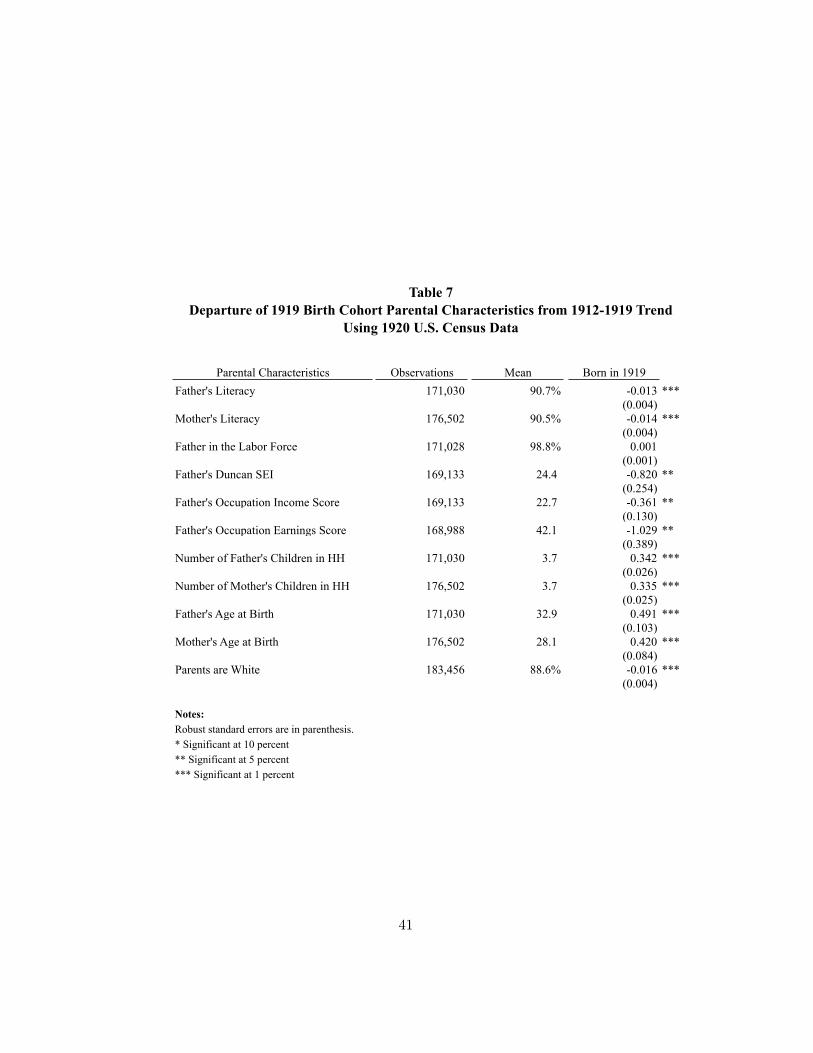
Table 7

Departure of 1919 Birth Cohort Parental Characteristics from 1912-1919 Trend

Using 1920 U.S. Census Data

Parental Characteristics Observations Mean Born in 1919

Father's Literacy d_litpN 171,030 blitpYRr 90.7% blitpr -0.013 *** blitpYRr2

plitpYRr plitpr (0.004) plitpYRr2

Mother's Literacy d_litmN 176,502 blitmYRr 90.5% blitmr -0.014 *** blitmYRr2

plitmYRr plitmr (0.004) plitmYRr2

Father in the Labor Force d_labfN 171,028 blabfYRr 98.8% blabfr 0.001 blabfYRr2

plabfYRr plabfr (0.001) plabfYRr2

Father's Duncan SEI seiN 169,133 bseiYR 24.4 bsei -0.820 ** bseiYR2

pseiYR psei (0.254) pseiYR2

Father's Occupation Income Score occN 169,133 boccYR 22.7 bocc -0.361 ** boccYR2

poccYR pocc (0.130) poccYR2

Father's Occupation Earnings Score erscorN 168,988 bersYR 42.1 bersc -1.029 ** bersYR2

persYR persc (0.389) persYR2

Number of Father's Children in HH chldpN 171,030 bchldpYR 3.7 bwhiter 0.342 *** bchldpYR2

pchldpYR (0.026) pchldpYR2

Number of Mother's Children in HH chldmN 176,502 bchldmYr 3.7 bwhitep 0.335 *** bchldmYr2

pchldmYR pwhitep (0.025) pchldmYR2

Father's Age at Birth aabpN 171,030 baabpYR 32.9 baabp 0.491 *** baabpYR2

paabpYR paabp (0.103) paabpYR2

Mother's Age at Birth aabmN 176,502 baabmYR 28.1 baabm 0.420 *** baabmYR2

paabmYR paabm (0.084) paabmYR2

Parents are White d_whiteN 183,456 bwhiYRr 88.6% bwhiter -0.016 *** bwhiYRr2

pwhiYRr pwhiter (0.004) pwhiYRr2

Notes:

Robust standard errors are in parenthesis.

* Significant at 10 percent

** Significant at 5 percent

*** Significant at 1 percent

41

Tab

le 8

Dep

art

ure

of

1919 B

irth

Coh

ort

by Q

uart

er P

are

nta

l C

hara

cter

isti

cs f

rom

1915-1

919 T

ren

d

Usi

ng 1

920 U

.S. C

ensu

s D

ata

Par

enta

l C

har

acte

rist

ics

Obse

rvat

ions

Mea

nB

orn

1Q

1919

Born

2Q

1919

Born

3Q

1919

Born

4Q

1919

Fat

her

's L

iter

acy

d_li

tpN107,8

36

bli

tp2Q

r91.0

%bli

tp2Q

r-0

.016

**

bli

tp3Q

r-0

.010

bli

tp4Q

r-0

.018

**

bli

tp5Q

r-0

.005

mean_lit_pop

pli

tp2Q

rpli

tp2Q

r(0.0

07)

pli

tp3Q

r(0.0

07)

pli

tp4Q

r(0.0

07)

pli

tp5Q

r(0.0

07)

Moth

er's

Lit

erac

yd_li

tmN1

11,1

43

bli

tm2Q

r90.9

%bli

tm2Q

r-0.0

27

***

bli

tm3Q

r-0.0

11

*bli

tm4Q

r-0.0

24

***

bli

tm5Q

r-0.0

10

mean_lit_mom

pli

tm2Q

rpli

tm2Q

r(0.0

07)

pli

tm3Q

r(0.0

07)

pli

tm4Q

r(0.0

07)

pli

tm5Q

r(0.0

07)

Fat

her

in t

he

Lab

or

Forc

ed_la

bfN

107,8

34

bla

bf2

Qr9

8.9

%bla

bf2

Qr-

0.0

04

*bla

bf3

Qr-

0.0

03

bla

bf4

Qr-

0.0

02

bla

bf5

Qr-

0.0

01

mean_labf_pop

pla

bf2

Qr

pla

bf2

Qr(0

.003)

pla

bf3

Qr(0

.002)

pla

bf4

Qr(0

.002)

pla

bf5

Qr(0

.002)

Fat

her

's D

unca

n S

EI

seiN

106,7

33

bse

i2Q

24.4

bse

i2Q

-1.2

81

**

bse

i3Q

-1.2

94

**

bse

i4Q

-1.1

29

**

bse

i5Q

-0.2

40

mean_sei_pop

pse

i2Q

pse

i2Q

(0.4

87)

pse

i3Q

(0.4

80)

pse

i4Q

(0.4

82)

pse

i5Q

(0.4

92)

Fat

her

's O

ccupat

ion I

nco

me

Sco

reocc

N106,7

33

bocc

2Q

22.8

bocc

2Q

-0.6

90

**

bocc

3Q

-0.7

45

**

bocc

4Q

-0.4

94

**

bocc

5Q

-0.2

63

mean_occ_pop

pocc

2Q

pocc

2Q

(0.2

48)

pocc

3Q

(0.2

44)

pocc

4Q

(0.2

46)

pocc

5Q

(0.2

50)

Fat

her

's O

ccupat

ion E

arnin

gs

Sco

reer

scorN

106,6

28

ber

s2Q

42.3

ber

s2Q

-1.9

37

**

ber

s3Q

-2.3

97

**

ber

s4Q

-1.2

38

*ber

s5Q

-0.3

78

mean_ersc

per

s2Q

per

s2Q

(0.7

42)

per

s3Q

(0.7

34)

per

s4Q

(0.7

38)

per

s5Q

(0.7

54)

Num

ber

of

Fat

her

's C

hil

dre

n i

n H

Hch

ldpN

107,8

36

bch

ldp2Q

3.4

bch

ldp2Q

0.2

95

***

bch

ldp3Q

0.4

39

***

bch

ldp4Q

0.4

28

***

bch

ldp5Q

0.3

29

***mean_chlp

pch

ldp2Q

pch

ldp2Q(0

.049)

pch

ldp3Q(0

.049)

pch

ldp4Q(0

.049)

pch

ldp5Q(0

.050)

Num

ber

of

Moth

er's

Chil

dre

n i

n H

Hch

ldm

N111,1

43

bch

ldm

2Q

3.4

bch

ldm

2Q0

.307

***

bch

ldm

3Q0

.434

***

bch

ldm

4Q0

.423

***

bch

ldm

5Q0

.343

***mean_chlm

pch

ldm

2Q

pch

ldm

2Q(0

.048)

pch

ldm

3Q(0

.048)

pch

ldm

4Q(0

.048)

pch

ldm

5Q(0

.049)

Fat

her

's A

ge

at B

irth

aabpN

107,8

36

baa

bp2Q

32.9

baa

bp2Q

0.4

22

**

baa

bp3Q

0.7

33

***

baa

bp4Q

0.6

60

***

baa

bp5Q

0.1

10

mean_aabp

paa

bp2Q

paa

bp2Q(

0.1

96)

paa

bp3Q(

0.1

94)

paa

bp4Q(

0.1

95)

paa

bp5Q(

0.2

00)

Moth

er's

Age

at B

irth

aabm

N111,1

43

baa

bm

2Q

28.1

baa

bm

2Q

0.4

35

**

baa

bm

3Q

0.5

73

***

baa

bm

4Q

0.3

70

**

baa

bm

5Q

0.0

83

mean_aabm

paa

bm

2Q

paa

bm

2Q(0

.160)

paa

bm

3Q(0

.158)

paa

bm

4Q(0

.157)

paa

bm

5Q(0

.162)

Par

ents

are

Whit

ed_w

hit

eN114,4

43

bw

hi2

Qr8

9.1

%bw

hi2

Qr-

0.0

27

***

bw

hi3

Qr-

0.0

23

**

bw

hi4

Qr-

0.0

20

**

bw

hi5

Qr-

0.0

03

mean_white

pw

hi2

Qr

pw

hi2

Qr(0

.007)

pw

hi3

Qr(0

.007)

pw

hi4

Qr(0

.007)

pw

hi5

Qr(0

.007)

No

tes:

Sp

ecif

icat

ion

in

clu

des

qu

arte

r o

f b

irth

fix

ed e

ffec

ts.

Ro

bu

st s

tan

dar

d e

rro

rs a

re i

n p

aren

thes

is.

* S

ign

ific

ant

at 1

0 p

erce

nt

**

Sig

nif

ican

t at

5 p

erce

nt

**

* S

ign

ific

ant

at 1

per

cen

t

42

Figure 4

-0.02

-0.015

-0.01

-0.005

0

0.005

0.01

0.015

1916 1917 1918 1919 1920

Quarter of Birth

Perc

en

t of

Lit

erate

Fath

ers

Note: Regression-adjusted 1920 literacy rate of fathers by quarter of child's birth.

43

Table 9

Departure of 1919 Birth Cohort Parental Characteristics from 1912-1922 Trend1

Using Combined 1920 and 1930 U.S. Census Data2

and Model to Account for Child's Age at Survey3

Parental Characteristics Observations Mean Born in 1919

Father's Literacy d_litpN 238,768 blitpr 92.0% blitpr -0.007 ** blitpr2

plitpr plitpr (0.003) plitpr2

Mother's Literacy d_litmN 250,778 blitmr 92.2% blitmr -0.005 * blitmr2

plitmr plitmr (0.003) plitmr2

Father in the Labor Force d_labfN 238,765 blabfr 98.0% blabfr 0.001 blabfr2

plabfr plabfr (0.001) plabfr2

Father's Duncan SEI seiN 235,282 bsei 25.5 burbanp -0.559 ** bsei2

psei purbanp (0.209) psei2

Father's Occupation Income Score occN 235,282 bocc 23.3 bwhiter -0.244 ** bocc2

pocc pwhiter (0.106) pocc2

Father's Occupation Earnings Score erscN 235,097 bersc 43.7 bwhitep -0.674 ** bersc2

persc pwhitep (0.320) persc2

Number of Father's Children in HH chldpN 238,768 bchldpr 3.8 bwhiter 0.212 *** bchldpr2

pchldpr pwhiter (0.021) pchldpr2

Number of Mother's Children in HH chldmN 250,778 bchldmr 3.8 bwhitep 0.214 *** bchldmr2

pchldmr pwhitep (0.021) pchldmr2

Father's Age at Birth aabpN 238,768 baabpp 32.5 baabp 0.571 *** baabp2

paabpp paabp (0.085) paabp2

Mother's Age at Birth aabmN 250,770 baabm 27.8 baabm 0.509 *** baabm2

paabm paabm (0.069) paabm2

Parents are White d_whiteN 273,457 bwhiter 88.0% bwhiter -0.005 bwhiter

pwhiter pwhiter (0.003) pwhiter

Notes:

Robust standard errors are in parenthesis.

* Significant at 10 percent

** Significant at 5 percent

*** Significant at 1 percent1Due to the timing of the 1930 U.S. Census, trend is from April 1, 1911 to March 31, 1923.2Data for people born between April 1, 1911 and March 31, 1915 or April 1, 1920 and March 31, 1923

is taken from 1930 U.S. Census. Data for people born between April 1, 1915 and December 31, 1919 is taken

from the 1920 U.S. Census. Data on people born between January 1, 1920 and March 31, 1920 is unavailable.3Model uses birth year, birth year squared, 1930 census year dummy, 1930 census year dummy interacted with

quadratic in age at survey, and 1919 birth cohort dummy as right hand side variables.

Age at survey was determined as the age of the child as of April 1st of the census year.

44

Table 10

Departure of 1919 Birth Cohort Parental Characteristics from 1913-1922 Trend1

Using Combined 1920 and 1930 U.S. Census Data2

and Model to Account for Child's Age at Survey3

Parental Characteristics Observations Mean Born in 1919

Father's Literacy d_litpN 223,528 blitpr 92.0% blitpr -0.007 ** blitpr2

plitpr plitpr (0.003) plitpr2

Mother's Literacy d_litmN 234,030 blitmr 92.2% blitmr -0.005 blitmr2

plitmr plitmr (0.003) plitmr2

Father in the Labor Force d_labfN 223,525 blabfr 98.1% blabfr 0.001 blabfr2

plabfr plabfr (0.001) plabfr2

Father's Duncan SEI seiN 220,515 bsei 25.4 burbanp -0.513 ** bsei2

psei purbanp (0.210) psei2

Father's Occupation Income Score occN 220,515 bocc 23.2 bwhiter -0.217 ** bocc2

pocc pwhiter (0.107) pocc2

Father's Occupation Earnings Score erscN 220,338 bersc 43.6 bwhitep -0.586 * bersc2

persc pwhitep (0.322) persc2

Number of Father's Children in HH chldpN 223,528 bchldpr 3.8 bwhiter 0.210 *** bchldpr2

pchldpr pwhiter (0.021) pchldpr2

Number of Mother's Children in HH chldmN 234,030 bchldmr 3.7 bwhitep 0.210 *** bchldmr2

pchldmr pwhitep (0.021) pchldmr2

Father's Age at Birth aabpN 223,528 baabpp 32.5 baabp 0.563 *** baabp2

paabpp paabp (0.085) paabp2

Mother's Age at Birth aabmN 234,027 baabm 27.8 baabm 0.520 *** baabm2

pMiss1r pwhitep (0.002) pMiss1r2

Parents are White d_whiteN 251,056 bwhiter 88.1% bwhiter -0.006 * bwhiter

pwhiter pwhiter (0.003) pwhiter

Notes:

Robust standard errors are in parenthesis.

* Significant at 10 percent

** Significant at 5 percent

*** Significant at 1 percent1Due to the timing of the 1930 U.S. Census, trend is from April 1, 1912 to March 31, 1923.2Data for people born between April 1, 1912 and March 31, 1915 or April 1, 1920 and March 31, 1923

is taken from 1930 U.S. Census. Data for people born between April 1, 1915 and December 31, 1919 is taken

from the 1920 U.S. Census. Data on people born between January 1, 1920 and March 31, 1920 is unavailable.3Model uses birth year, birth year squared, 1930 census year dummy, 1930 census year dummy interacted with

quadratic in age at survey, and 1919 birth cohort dummy as right hand side variables.

Age at survey was determined as the age of the child as of April 1st of the census year.

45

Table 11

Departure of 1919 Male Birth Cohort Parental Characteristics from 1912-1922 Male Trend1

Using Combined 1920 and 1930 U.S. Census Data2

and Model to Account for Child's Age at Survey3

Parental Characteristics Observations Mean Born in 1919

Father's Literacy d_litpN 122,612 blitpr 92.1% blitpr -0.009 ** blitpr2

plitpr plitpr (0.004) plitpr2

Mother's Literacy d_litmN 128,561 blitmr 92.3% blitmr -0.007 * blitmr2

plitmr plitmr (0.004) plitmr2

Father in the Labor Force d_labfN 122,611 blabfr 98.0% blabfr 0.001 blabfr2

plabfr plabfr (0.002) plabfr2

Father's Duncan SEI seiN 120,866 bsei 25.4 burbanp -0.822 ** bsei2

psei purbanp (0.293) psei2

Father's Occupation Income Score occN 120,866 bocc 23.2 bwhiter -0.329 ** bocc2

pocc pwhiter (0.148) pocc2

Father's Occupation Earnings Score erscN 120,777 bersc 43.6 bwhitep -0.946 ** bersc2

persc pwhitep (0.447) persc2

Number of Father's Children in HH chldpN 122,612 bchldpr 3.8 bwhiter 0.222 *** bchldpr2

pchldpr pwhiter (0.030) pchldpr2

Number of Mother's Children in HH chldmN 128,561 bchldmr 3.8 bwhitep 0.223 *** bchldmr2

pchldmr pwhitep (0.029) pchldmr2

Father's Age at Birth aabpN 122,612 baabpp 32.4 baabp 0.575 *** baabp2

paabpp paabp (0.118) paabp2

Mother's Age at Birth aabmN 128,558 baabm 27.8 baabm 0.512 *** baabm2

paabm paabm (0.096) paabm2

Parents are White d_whiteN 138,575 bwhiter 88.3% bwhiter -0.009 ** bwhiter

pwhiter pwhiter (0.004) pwhiter

Notes:

Robust standard errors are in parenthesis.

* Significant at 10 percent

** Significant at 5 percent

*** Significant at 1 percent1Due to the timing of the 1930 U.S. Census, trend is from April 1, 1911 to March 31, 1923.2Data for people born between April 1, 1911 and March 31, 1915 or April 1, 1920 and March 31, 1923

is taken from 1930 U.S. Census. Data for people born between April 1, 1915 and December 31, 1919 is taken

from the 1920 U.S. Census. Data on people born between January 1, 1920 and March 31, 1920 is unavailable.3Model uses birth year, birth year squared, 1930 census year dummy, 1930 census year dummy interacted with

quadratic in age at survey, and 1919 birth cohort dummy as right hand side variables.

Age at survey was determined as the age of the child as of April 1st of the census year.

46

Ta

ble

12

An

aly

sis

of

the

Ma

gn

itu

de

an

d S

ign

ific

an

ce o

f th

e A

lmo

nd

20

06

Est

ima

tes

of

the

Imp

act

of

Bei

ng

Bo

rn i

n 1

91

9 f

or

Men

Wh

en A

dd

ing

Pla

ce o

f B

irth

In

dic

ato

rs,

a R

ace

In

dic

ato

r, a

s w

ell

as

thei

r In

tera

ctio

n1

1960 U

.S. C

ensu

s1970 U

.S. C

ensu

s1980 U

.S. C

ensu

s

Long-T

erm

Outc

om

eM

agnit

ude

Red

uct

ion

2S

till

Sig

. at

5%

3M

agnit

ude

Red

uct

ion

2S

till

Sig

. at

5%

3M

agnit

ude

Red

uct

ion

2S

till

Sig

. at

5%

3

Hig

h S

chool

Gra

duat

e!"#$%&'(

26%

YE

S!"#$%&'(

33%

YE

S!"#$%&'(

41%

YE

S

Yea

rs o

f E

duca

tion

!)*$%&(

40%

YE

S!)*$%&(

35%

YE

S!)*$%&(

46%

YE

S

Tota

l In

com

e!*+,-.-(

62%

n/a

!*+,-.-(

46%

YE

S!*+,-.-(

27%

YE

S

Wag

e In

com

e!*+,/

&$(

48%

NO

!*+,/

&$(

44%

YE

S!*+,/

&$(

28%

YE

S

Poor

(bel

ow

150%

of

the

pover

ty l

evel

)!'0..%(

52%

NO

!'0..%(

47%

YE

S!'0..%(

86%

NO

Nei

ghbors

' Inco

me

!12*(

!32'*(

41%

YE

S!12*(

Dunca

n's

Soci

oec

onom

ic I

ndex

!12*(

41%

NO

!12*(

35%

YE

S!12*(

36%

NO

Dis

abil

ity L

imit

s W

ork

bdli

mM

19%

YE

Sbdli

mM

35%

NO

Dis

abil

ity P

reven

ts W

ork

bdprv

M46%

NO

4bdprv

M92%

n/a

Soci

al S

ecuri

ty I

nco

me

bin

cssM

955%

n/a

bin

cssM

-7%

YE

S

Wel

fare

Inco

me

bin

cwel

M23%

NO

5bin

cwel

M33%

NO

6

Note

s:

Com

par

ison r

egre

ssio

ns

use

the

sam

e m

odel

s as

in A

lmond's

2006 p

aper

and d

ata

is t

aken

fro

m I

PU

MS

sam

ple

note

d i

n t

he

colu

mn h

eader

.

IPU

MS

dat

a use

d f

or

all

regre

ssio

ns

was

cle

aned

of

resp

onden

ts b

orn

outs

ide

the

U.S

. an

d n

o v

alue

wit

h a

qual

ity f

lag a

bove

3 i

s use

d (

i.e.

"hot

dec

k"

and "

cold

dec

k"

allo

cate

d v

alues

are

not

use

d).

1A

dum

my v

aria

ble

for

whet

her

the

resp

onden

t w

as w

hit

e w

as u

sed a

s th

e ra

ce i

ndic

ator.

2R

educt

ion i

s ca

lcula

ted a

s (O

rig. C

oef

f. -

New

Coef

f.)/

(Ori

g. C

oef

f.).

N

egat

ive

reduct

ion i

ndic

ates

the

poin

t es

tim

ate

bec

ame

larg

er i

n a

bso

lute

ter

ms.

3"Y

ES

"/"N

O"

indic

ates

whet

her

bei

ng b

orn

in 1

919 r

emai

ned

sig

nif

ican

t at

or

bel

ow

the

5%

lev

el i

n t

he

fixed

eff

ect

spec

ific

atio

n o

f A

lmond's

model

. "

n/a

" in

dic

ates

that

the

1919 d

um

my v

aria

ble

was

not

signif

ican

t in

Alm

ond's

ori

gin

al s

pec

ific

atio

n.

4W

hen

lim

itin

g t

o o

nly

hig

her

qual

ity v

alues

, th

e re

pli

cate

d n

on-f

ixed

eff

ect

regre

ssio

n n

o l

onger

was

sig

nif

ican

t at

or

bel

ow

the

5%

lev

el a

s in

the

Alm

ond 2

006 p

aper

(p-v

alue

of

repli

cati

on i

s .0

9).

The

fixed

eff

ects

spec

ific

atio

n f

urt

her

incr

ease

s th

e p-v

alue

to .35.

5A

s in

footn

ote

4, re

pli

cati

on o

f A

lmond's

reg

ress

ion g

ives

p-v

alue

no l

onger

at

or

bel

ow

.05 (

p-v

alue

of

repli

cati

on i

s .0

6).

T

he

fixed

eff

ects

spec

ific

atio

n f

urt

her

incr

ease

s th

e p-v

alue

to .14.

6A

s in

footn

ote

4, re

pli

cati

on o

f A

lmond's

reg

ress

ion g

ives

p-v

alue

no l

onger

at

or

bel

ow

.05 (

p-v

alue

of

repli

cati

on i

s .0

7).

T

he

fixed

eff

ects

spec

ific

atio

n f

urt

her

incr

ease

s th

e p-v

alue

to .30.

47

Ta

ble

13

An

aly

sis

of

the

Ma

gn

itu

de

an

d S

ign

ific

an

ce o

f th

e A

lmo

nd

20

06

Est

ima

tes

of

the

Imp

act

of

Bei

ng

Bo

rn i

n 1

91

9 f

or

Wo

men

Wh

en A

dd

ing

Pla

ce o

f B

irth

In

dic

ato

rs,

a R

ace

In

dic

ato

r, a

s w

ell

as

thei

r In

tera

ctio

n1

1960 U

.S. C

ensu

s1970 U

.S. C

ensu

s1980 U

.S. C

ensu

s

Long-T

erm

Outc

om

eM

agnit

ude

Red

uct

ion

2S

till

Sig

. at

5%

3M

agnit

ude

Red

uct

ion

2S

till

Sig

. at

5%

3M

agnit

ude

Red

uct

ion

2S

till

Sig

. at

5%

3

Hig

h S

chool

Gra

duat

e!"#$%&'(

29%

YE

S!"#$%&'(

32%

YE

S!"#$%&'(

35%

YE

S

Yea

rs o

f E

duca

tion

!)*$%&(

40%

YE

S!)*$%&(

38%

YE

S!)*$%&(

54%

YE

S

Tota

l In

com

e!*+,-.-(

-21%

Oth

er4

!*+,-.-(

34%

n/a

!*+,-.-(

24%

YE

S

Wag

e In

com

e!*+,/

&$(

-57%

n/a

!*+,/

&$(

53%

n/a

!*+,/

&$(

36%

n/a

Poor

(bel

ow

150%

of

the

pover

ty l

evel

)!'0..%(

64%

NO

!'0..%(

57%

NO

!'0..%(

70%

NO

7

Nei

ghbors

' Inco

me

!12*(

!32'*(

73%

NO

!12*(

Dunca

n's

Soci

oec

onom

ic I

ndex

!12*(

60%

NO

5!12*(

50%

NO

!12*(

41%

YE

S

Dis

abil

ity L

imit

s W

ork

bdli

mM

71%

n/a

bdli

mM

72%

n/a

Dis

abil

ity P

reven

ts W

ork

bdprv

M47%

NO

6bdprv

M71%

n/a

Soci

al S

ecuri

ty I

nco

me

bin

cssM

158%

n/a

bin

cssM

6%

YE

S8

Wel

fare

Inco

me

bin

cwel

M36%

NO

bin

cwel

M64%

n/a

Note

s:

Com

par

ison r

egre

ssio

ns

use

the

sam

e m

odel

s as

in A

lmond's

2006 p

aper

and d

ata

is t

aken

fro

m I

PU

MS

sam

ple

note

d i

n t

he

colu

mn h

eader

.

IPU

MS

dat

a use

d f

or

all

regre

ssio

ns

was

cle

aned

of

resp

onden

ts b

orn

outs

ide

the

U.S

. an

d n

o v

alue

wit

h a

qual

ity f

lag a

bove

3 i

s use

d (

i.e.

"hot

dec

k"

and "

cold

dec

k"

allo

cate

d v

alues

are

not

use

d).

1A

dum

my v

aria

ble

for

whet

her

the

resp

onden

t w

as w

hit

e w

as u

sed a

s th

e ra

ce i

ndic

ator.

2R

educt

ion i

s ca

lcula

ted a

s (O

rig. C

oef

f. -

New

Coef

f.)/

(Ori

g. C

oef

f.).

N

egat

ive

reduct

ion i

ndic

ates

the

poin

t es

tim

ate

bec

ame

larg

er i

n a

bso

lute

ter

ms.

3"Y

ES

"/"N

O"

indic

ates

whet

her

bei

ng b

orn

in 1

919 r

emai

ned

sig

nif

ican

t at

or

bel

ow

the

5%

lev

el i

n t

he

fixed

eff

ect

spec

ific

atio

n o

f A

lmond's

model

. "

n/a

" in

dic

ates

that

the

1919 d

um

my v

aria

ble

was

not

signif

ican

t in

Alm

ond's

ori

gin

al s

pec

ific

atio

n.

4In

Alm

ond 2

006 t

ota

l in

com

e is

sig

nif

ican

t at

the

10%

lev

el, but

the

sign o

f th

e co

effi

cien

t, c

ontr

adic

ting h

is h

ypoth

esis

, is

posi

tive.

U

sing t

he

fixed

eff

ects

spec

ific

atio

n

the

poin

t es

tim

ate

rem

ains

posi

tive

and b

ecom

es s

ignif

ican

t at

the

5%

lev

el.

5W

hen

lim

itin

g t

o o

nly

hig

her

qual

ity v

alues

, th

e re

pli

cate

d n

on-f

ixed

eff

ect

regre

ssio

n w

as s

ignif

ican

t at

the

5%

lev

el, w

hil

e in

the

Alm

ond 2

006 p

aper

it

was

not.

T

he

fixed

eff

ects

spec

ific

atio

n i

ncr

ease

s th

e p-v

alue

to .31.

6W

hen

lim

itin

g t

o o

nly

hig

her

qual

ity v

alues

, th

e re

pli

cate

d n

on-f

ixed

eff

ect

regre

ssio

n n

o l

onger

was

sig

nif

ican

t at

or

bel

ow

the

5%

lev

el a

s in

the

Alm

ond 2

006 p

aper

(p-v

alue

of

repli

cati

on i

s .1

6).

The

fixed

eff

ects

spec

ific

atio

n f

urt

her

incr

ease

s th

e p-v

alue

to .45.

7A

s in

footn

ote

5, th

e re

pli

cate

d n

on-f

ixed

eff

ect

regre

ssio

n w

as s

ignif

ican

t at

the

5%

lev

el, w

hil

e in

the

Alm

ond 2

006 p

aper

it

was

not.

T

he

fixed

eff

ects

spec

ific

atio

n i

ncr

ease

s th

e p-v

alue

to .34.

8In

Alm

ond 2

006 S

S i

nco

me

is s

ignif

ican

t at

or

bel

ow

the

5%

lev

el, but

the

sign o

f th

e co

effi

cien

t, c

ontr

adic

ting h

is h

ypoth

esis

, is

neg

ativ

e. U

sing t

he

fixed

eff

ects

spec

ific

atio

n

the

poin

t es

tim

ate

rem

ains

neg

ativ

e an

d s

ignif

ican

t at

or

bel

ow

the

5%

lev

el.

48

XI Appendix

49

Table A1

Departure of 1919 Birth Cohort1 Parental Characteristics from 1912-1922 Trend

2

Using 1930 U.S. Census Data and Alternative Specification3

Parental Characteristics Observations Mean Born in 19191

Father's Literacy d_litpN 237,785 blitpr 92.8% blitpr -0.002 blitpr2

plitpr plitpr (0.002) plitpr2

Mother's Literacy d_litmN 252,565 blitmr 93.1% blitmr -0.003 blitmr2

plitmr plitmr (0.002) plitmr2

Father in the Labor Force d_labfN 237,783 blabfr 97.5% blabfr -0.001 blabfr2

plabfr plabfr (0.001) plabfr2

Father's Duncan SEI seiN 233,865 bsei 26.2 bsei -0.356 ** bsei2

psei psei (0.155) psei2

Father's Occupation Income Score occN 233,865 bocc 23.6 bocc -0.174 ** bocc2

pocc pocc (0.076) pocc2

Father's Occupation Earnings Score erscN 233,714 bersc 44.6 bersc -0.410 * bersc2

persc persc (0.225) persc2

Parents Own a Radio d_radioN 281,463 bradior 34.6% bradior -0.010 ** bradior2

pradior pradior (0.003) pradior2

Number of Father's Children in HH chldpN 237,785 bchldpr 4.1 bwhiter 0.118 *** bchldpr2

pchldpr pwhiter (0.015) pchldpr2

Number of Mother's Children in HH chldmN 252,565 bchldmr 4.1 bwhitep 0.121 *** bchldmr2

pchldmr pwhitep (0.015) pchldmr2

Father's Age at Birth aabpN 237,785 baabpp 32.1 baabp 0.226 *** baabp2

paabpp paabp (0.058) paabp2

Mother's Age at Birth aabmN 252,556 baabm 27.6 baabm 0.225 *** baabm2

paabm paabm (0.049) paabm2

Father's a WWI Veteran d_WW1N237,785 bWW1r 6.9% bWW1r -0.027 *** bWW1r2

pWW1r pWW1r (0.002) pWW1r2

Parents are White d_whiteN 281,463 bwhiter 87.6% bwhiter -0.004 * bwhiter2

pwhiter pwhiter (0.002) pwhiter2

Notes:

Robust standard errors are in parenthesis.

* Significant at 10 percent

** Significant at 5 percent

*** Significant at 1 percent1Due to the timing of the 1930 U.S. Census, 1919 birth cohort consists of people born between

April 1, 1919 and March 31, 1920.2Due to the timing of the 1930 U.S. Census, trend is from April 1, 1911 to March 31, 1923.3Model excludes quadratic in year of birth.

50

Table A2

Departure of 1919 Birth Cohort1 Parental Characteristics from 1913-1922 Trend

2

Using 1930 U.S. Census Data and Alternative Specification3

Parental Characteristics Observations Mean Born in 19191

Father's Literacy d_litpN 222,545 blitpr 92.8% blitpr -0.002 blitpr2

plitpr plitpr (0.002) plitpr2

Mother's Literacy d_litmN 235,817 blitmr 93.2% blitmr -0.003 blitmr2

plitmr plitmr (0.002) plitmr2

Father in the Labor Force d_labfN 222,543 blabfr 97.6% blabfr -0.001 blabfr2

plabfr plabfr (0.001) plabfr2

Father's Duncan SEI seiN 219,098 bsei 26.2 bsei -0.360 ** bsei2

psei psei (0.155) psei2

Father's Occupation Income Score occN 219,098 bocc 23.6 bocc -0.176 ** bocc2

pocc pocc (0.076) pocc2

Father's Occupation Earnings Score erscN 218,955 bersc 44.6 bersc -0.416 * bersc2

persc persc (0.225) persc2

Parents Own a Radio d_radioN 259,062 bradior 34.4% bradior -0.010 ** bradior2

pradior pradior (0.003) pradior2

Number of Father's Children in HH chldpN 222,545 bchldpr 4.1 bwhiter 0.119 *** bchldpr2

pchldpr pwhiter (0.015) pchldpr2

Number of Mother's Children in HH chldmN 235,817 bchldmr 4.1 bwhitep 0.123 *** bchldmr2

pchldmr pwhitep (0.015) pchldmr2

Father's Age at Birth aabpN 222,545 baabpp 32.1 baabp 0.225 *** baabp2

paabpp paabp (0.058) paabp2

Mother's Age at Birth aabmN 235,813 baabm 27.6 baabm 0.224 *** baabm2

paabm paabm (0.049) paabm2

Father's a WWI Veteran d_WW1N222,545 bWW1r 7.2% bWW1r -0.027 *** bWW1r2

pWW1r pWW1r (0.002) pWW1r2

Parents are White d_whiteN 259,062 bwhiter 87.7% bwhiter -0.004 bwhiter2

pwhiter pwhiter (0.002) pwhiter2

Notes:

Robust standard errors are in parenthesis.

* Significant at 10 percent

** Significant at 5 percent

*** Significant at 1 percent1Due to the timing of the 1930 U.S. Census, 1919 birth cohort consists of people born between

April 1, 1919 and March 31, 1920.2Due to the timing of the 1930 U.S. Census, trend is from April 1, 1912 to March 31, 1923.3Model excludes quadratic in year of birth.

51

Table A3

Departure of 1919 Male Birth Cohort1 Parental Characteristics from 1912-1922 Male Trend

2

Using 1930 U.S. Census Data and Alternative Specification3

Parental Characteristics Observations Mean Born in 19191

Father's Literacy d_litpN 121,164 blitpr 92.8% blitpr -0.002 blitpr2

plitpr plitpr (0.003) plitpr2

Mother's Literacy d_litmN 128,431 blitmr 93.1% blitmr -0.003 blitmr2

plitmr plitmr (0.003) plitmr2

Father in the Labor Force d_labfN 121,164 blabfr 97.5% blabfr 0.000 blabfr2

plabfr plabfr (0.001) plabfr2

Father's Duncan SEI seiN 119,197 bsei 26.1 bsei -0.247 bsei2

psei psei (0.218) psei2

Father's Occupation Income Score occN 119,197 bocc 23.5 bocc -0.204 * bocc2

pocc pocc (0.106) pocc2

Father's Occupation Earnings Score erscN 119,121 bersc 44.3 bersc -0.456 bersc2

persc persc (0.317) persc2

Parents Own a Radio d_radioN 141,658 bradior 34.8% bradior -0.015 *** bradior2

pradior pradior (0.005) pradior2

Number of Father's Children in HH chldpN 121,164 bchldpr 4.1 bwhiter 0.136 *** bchldpr2

pchldpr pwhiter (0.021) pchldpr2

Number of Mother's Children in HH chldmN 128,431 bchldmr 4.1 bwhitep 0.137 *** bchldmr2

pchldmr pwhitep (0.021) pchldmr2

Father's Age at Birth aabpN 121,164 baabpp 32.1 baabp 0.211 ** baabp2

paabpp paabp (0.081) paabp2

Mother's Age at Birth aabmN 128,427 baabm 27.6 baabm 0.208 ** baabm2

paabm paabm (0.069) paabm2

Father's a WWI Veteran d_WW1N 121,164 bWW1r 6.8% bWW1r -0.027 *** bWW1r2

pWW1r pWW1r (0.003) pWW1r2

Parents are White d_whiteN 141,658 bwhiter 87.8% bwhiter -0.008 ** bwhiter2

pwhiter pwhiter (0.003) pwhiter2

Notes:

Robust standard errors are in parenthesis.

* Significant at 10 percent

** Significant at 5 percent

*** Significant at 1 percent1Due to the timing of the 1930 U.S. Census, 1919 birth cohort consists of people born between

April 1, 1919 and March 31, 1920.2Due to the timing of the 1930 U.S. Census, trend is from April 1, 1911 to March 31, 1923.3Model excludes quadratic in year of birth.

52

Ta

ble

A4

Dep

art

ure

of

Wh

ite

Fa

ther

s a

nd

Wo

rld

Wa

r I

Vet

era

n F

ath

ers

fro

m A

ll F

ath

ers

in 1

91

2 t

o 1

92

21

Usi

ng

19

30

U.S

. C

ensu

s D

ata

Par

enta

l C

har

acte

rist

ics

Obse

rvat

ions

Mea

nW

hit

eW

WI

Vet

eran

Fat

her

's L

iter

acy

d_li

tpN

237,7

85

bli

tpr

92.8

%bli

tpr

0.1

61

***

bli

tpr

0.0

30

***

bli

tpr2

pli

tpr

pli

tpr

(0.0

03)

pli

tpr

(0.0

01)

pli

tpr2

Fat

her

's D

unca

n S

EI

seiN

233,8

65

bse

i26.2

bse

i11.0

40

***

bse

i6.5

03

***

bse

i2

pse

ipse

i(0

.114)

pse

i(0

.195)

pse

i2

Fat

her

's O

ccupat

ion I

nco

me

Sco

reocc

N233,8

65

bocc

23.6

bocc

4.9

85

***

bocc

2.9

55

***

bocc

2

pocc

pocc

(0.0

61)

pocc

(0.0

95)

pocc

2

Fat

her

's O

ccupat

ion E

arnin

gs

Sco

reer

scN

233,7

14

ber

sc44.6

ber

sc13.6

18

***

ber

sc7.9

05

***

ber

sc2

per

scper

sc(0

.186)

per

sc(0

.240)

per

sc2

Par

ents

Ow

n a

Rad

iod_ra

dio

N281,4

63

bra

dio

r34.6

%bra

dio

r0.1

55

***

bra

dio

r0.0

93

***

bra

dio

r2

pra

dio

rpra

dio

r(0

.002)

pra

dio

r(0

.004)

pra

dio

r2

Num

ber

of

Fat

her

's C

hil

dre

n i

n H

Hch

ldpN

237,7

85

bch

ldpr

4.1

bw

hit

er-0

.574

***

bw

hit

er-0

.850

***

bch

ldpr2

pch

ldpr

pw

hit

er(0

.017)

pw

hit

er(0

.014)

pch

ldpr2

No

tes:

Ro

bu

st s

tan

dar

d e

rro

rs a

re i

n p

aren

thes

is.

* S

ign

ific

ant

at 1

0 p

erce

nt

**

Sig

nif

ican

t at

5 p

erce

nt

**

* S

ign

ific

ant

at 1

per

cen

t1D

ue

to t

he

tim

ing

of

the

19

30

U.S

. C

ensu

s, t

ren

d i

s fr

om

Ap

ril

1,

19

11

to

Mar

ch 3

1,

19

23

.

Sp

ecif

icat

ion

use

s ag

e o

f fa

ther

, ag

e o

f fa

ther

sq

uar

ed,

stat

e o

f b

irth

fix

ed e

ffec

ts,

du

mm

y f

or

wh

ite,

an

d d

um

my

fo

r W

WI

vet

eran

as

the

rig

ht

han

d s

ide

var

iab

les.

53

Table A5

Departure of 1917 Birth Cohort1 Parental Characteristics from 1912-1922 Trend

2

Using 1930 U.S. Census Data

Parental Characteristics Observations Mean Born in 19171

Father's Literacy d_litpN 237,785 blitpr 92.8% blitpr 0.000 blitpr2

plitpr plitpr (0.002) plitpr2

Mother's Literacy d_litmN 252,565 blitmr 93.1% blitmr -0.003 blitmr2

plitmr plitmr (0.002) plitmr2

Father in the Labor Force d_labfN 237,783 blabfr 97.5% blabfr 0.000 blabfr2

plabfr plabfr (0.001) plabfr2

Father's Duncan SEI seiN 233,865 bsei 26.2 bsei -0.031 bsei2

psei psei (0.165) psei2

Father's Occupation Income Score occN 233,865 bocc 23.6 bocc -0.042 bocc2

pocc pocc (0.081) pocc2

Father's Occupation Earnings Score erscN 233,714 bersc 44.6 bersc -0.133 bersc2

persc persc (0.239) persc2

Parents Own a Radio d_radioN 281,463 bradior 34.6% bradior 0.004 bradior2

pradior pradior (0.003) pradior2

Number of Father's Children in HH chldpN 237,785 bchldpr 4.1 bwhiter 0.008 bchldpr2

pchldpr pwhiter (0.016) pchldpr2

Number of Mother's Children in HH chldmN 252,565 bchldmr 4.1 bwhitep 0.001 bchldmr2

pchldmr pwhitep (0.016) pchldmr2

Father's Age at Birth aabpN 237,785 baabpp 32.1 baabp -0.124 ** baabp2

paabpp paabp (0.060) paabp2

Mother's Age at Birth aabmN 252,556 baabm 27.6 baabm -0.062 baabm2

paabm paabm (0.052) paabm2

Father's a WWI Veteran d_WW1N237,785 bWW1r 6.9% bWW1r -0.015 *** bWW1r2

pWW1r pWW1r (0.001) pWW1r2

Parents are White d_whiteN 281,463 bwhiter 87.6% bwhiter -0.005 ** bwhiter2

pwhiter pwhiter (0.002) pwhiter2

Notes:

Robust standard errors are in parenthesis.

* Significant at 10 percent

** Significant at 5 percent

*** Significant at 1 percent1Due to the timing of the 1930 U.S. Census, 1917 birth cohort consists of people born between

April 1, 1917 and March 31, 1918.2Due to the timing of the 1930 U.S. Census, trend is from April 1, 1911 to March 31, 1923.

54

Table A6

Departure of 1920 Birth Cohort1 Parental Characteristics from 1912-1922 Trend

2

Using 1930 U.S. Census Data

Parental Characteristics Observations Mean Born in 19201

Father's Literacy d_litpN 237,785 blitpr 92.8% blitpr 0.001 blitpr2

plitpr plitpr (0.002) plitpr2

Mother's Literacy d_litmN 252,565 blitmr 93.1% blitmr 0.003 blitmr2

plitmr plitmr (0.002) plitmr2

Father in the Labor Force d_labfN 237,783 blabfr 97.5% blabfr 0.001 blabfr2

plabfr plabfr (0.001) plabfr2

Father's Duncan SEI seiN 233,865 bsei 26.2 bsei 0.208 bsei2

psei psei (0.159) psei2

Father's Occupation Income Score occN 233,865 bocc 23.6 bocc 0.137 * bocc2

pocc pocc (0.078) pocc2

Father's Occupation Earnings Score erscN 233,714 bersc 44.6 bersc 0.431 * bersc2

persc persc (0.228) persc2

Parents Own a Radio d_radioN 281,463 bradior 34.6% bradior 0.009 ** bradior2

pradior pradior (0.003) pradior2

Number of Father's Children in HH chldpN 237,785 bchldpr 4.1 bwhiter -0.061 *** bchldpr2

pchldpr pwhiter (0.015) pchldpr2

Number of Mother's Children in HH chldmN 252,565 bchldmr 4.1 bwhitep -0.063 *** bchldmr2

pchldmr pwhitep (0.015) pchldmr2

Father's Age at Birth aabpN 237,785 baabpp 32.1 baabp -0.191 ** baabp2

paabpp paabp (0.059) paabp2

Mother's Age at Birth aabmN 252,556 baabm 27.6 baabm -0.108 ** baabm2

paabm paabm (0.050) paabm2

Father's a WWI Veteran d_WW1N237,785 bWW1r 6.9% bWW1r 0.034 *** bWW1r2

pWW1r pWW1r (0.003) pWW1r2

Parents are White d_whiteN 281,463 bwhiter 87.6% bwhiter -0.002 bwhiter2

pwhiter pwhiter (0.002) pwhiter2

Notes:

Robust standard errors are in parenthesis.

* Significant at 10 percent

** Significant at 5 percent

*** Significant at 1 percent1Due to the timing of the 1930 U.S. Census, 1920 birth cohort consists of people born between

April 1, 1920 and March 31, 1921.2Due to the timing of the 1930 U.S. Census, trend is from April 1, 1911 to March 31, 1923.

55

Table B1

Departure of 1919 Birth Cohort Parental Characteristics from 1912-1919 Trend

Using 1920 U.S. Census Data and Alternative Specification1

Parental Characteristics Observations Mean Born in 1919

Father's Literacy d_litpN 171,030 blitpYRr 90.7% blitpr -0.007 ** blitpYRr2

plitpYRr plitpr (0.003) plitpYRr2

Mother's Literacy d_litmN 176,502 blitmYRr 90.5% blitmr -0.003 blitmYRr2

plitmYRr plitmr (0.003) plitmYRr2

Father in the Labor Force d_labfN 171,028 blabfYRr 98.8% blabfr -0.001 blabfYRr2

plabfYRr plabfr (0.001) plabfYRr2

Father's Duncan SEI seiN 169,133 bseiYR 24.4 bsei -0.646 *** bseiYR2

pseiYR psei (0.178) pseiYR2

Father's Occupation Income Score occN 169,133 boccYR 22.7 bocc -0.356 *** boccYR2

poccYR pocc (0.091) poccYR2

Father's Occupation Earnings Score erscorN 168,988 bersYR 42.1 bersc -0.979 *** bersYR2

persYR persc (0.274) persYR2

Number of Father's Children in HH chldpN 171,030 bchldpYR 3.7 bwhiter 0.176 *** bchldpYR2

pchldpYR (0.018) pchldpYR2

Number of Mother's Children in HH chldmN 176,502 bchldmYr 3.7 bwhitep 0.177 *** bchldmYr2

pchldmYR pwhitep (0.018) pchldmYR2

Father's Age at Birth aabpN 171,030 baabpYR 32.9 baabp 0.527 *** baabpYR2

paabpYR paabp (0.073) paabpYR2

Mother's Age at Birth aabmN 176,502 baabmYR 28.1 baabm 0.418 *** baabmYR2

paabmYR paabm (0.059) paabmYR2

Parents are White d_whiteN 183,456 bwhiYRr 88.6% bwhiter -0.013 *** bwhiYRr2

pwhiYRr pwhiter (0.003) pwhiYRr2

Notes:

Robust standard errors are in parenthesis.

* Significant at 10 percent

** Significant at 5 percent

*** Significant at 1 percent1Model excludes quadratic in year of birth.

56

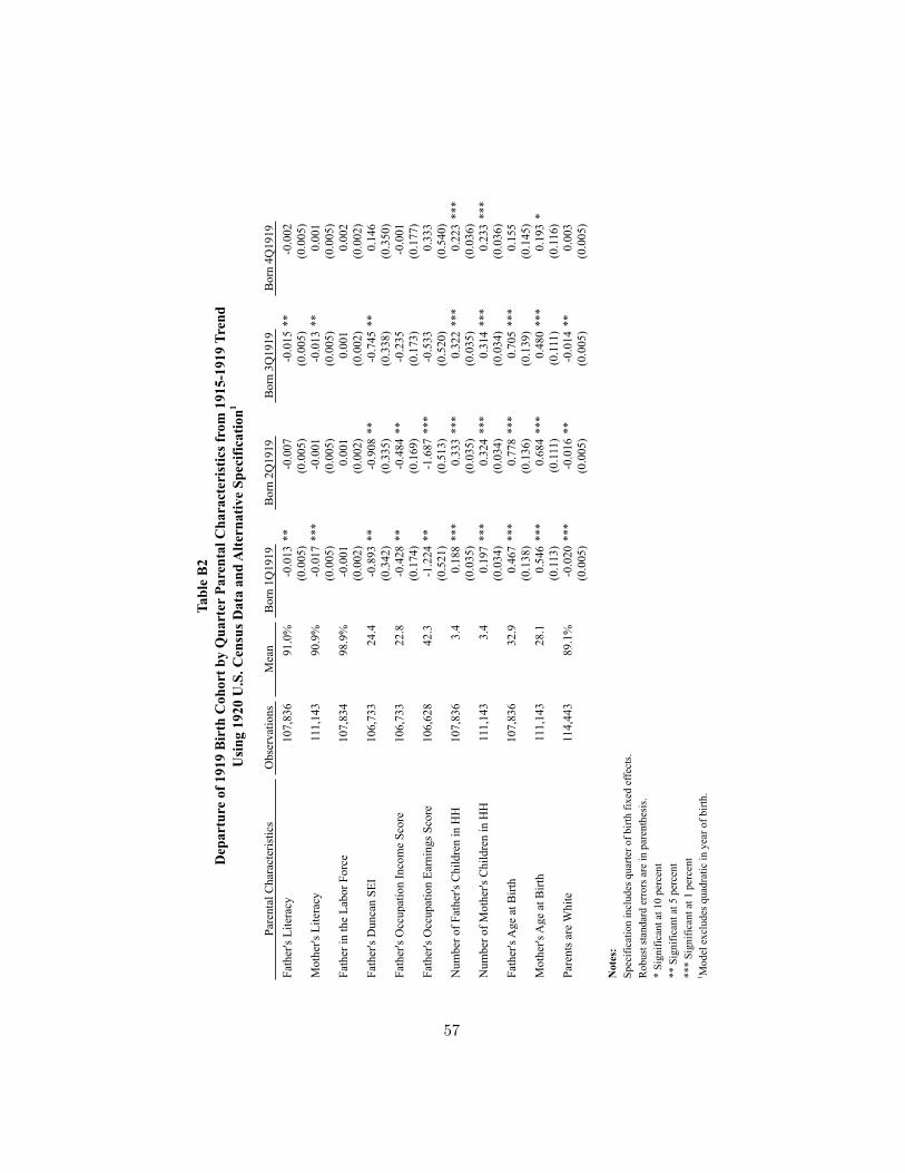
Tab

le B

2

Dep

art

ure

of

1919 B

irth

Coh

ort

by Q

uart

er P

are

nta

l C

hara

cter

isti

cs f

rom

1915-1

919 T

ren

d

Usi

ng 1

920 U

.S. C

ensu

s D

ata

an

d A

lter

nati

ve

Sp

ecif

icati

on

1

Par

enta

l C

har

acte

rist

ics

Obse

rvat

ions

Mea

nB

orn

1Q

1919

Born

2Q

1919

Born

3Q

1919

Born

4Q

1919

Fat

her

's L

iter

acy

d_li

tpN107,8

36

bli

tp2Q

r91.0

%bli

tp2Q

r-0

.013

**

bli

tp3Q

r-0

.007

bli

tp4Q

r-0

.015

**

bli

tp5Q

r-0

.002

mean_lit_pop

pli

tp2Q

rpli

tp2Q

r(0.0

05)

pli

tp3Q

r(0.0

05)

pli

tp4Q

r(0.0

05)

pli

tp5Q

r(0.0

05)

Moth

er's

Lit

erac

yd_li

tmN1

11,1

43

bli

tm2Q

r90.9

%bli

tm2Q

r-0.0

17

***

bli

tm3Q

r-0.0

01

bli

tm4Q

r-0.0

13

**

bli

tm5Q

r0.0

01

mean_lit_mom

pli

tm2Q

rpli

tm2Q

r(0.0

05)

pli

tm3Q

r(0.0

05)

pli

tm4Q

r(0.0

05)

pli

tm5Q

r(0.0

05)

Fat

her

in t

he

Lab

or

Forc

ed_la

bfN

107,8

34

bla

bf2

Qr9

8.9

%bla

bf2

Qr-

0.0

01

bla

bf3

Qr

0.0

01

bla

bf4

Qr

0.0

01

bla

bf5

Qr

0.0

02

mean_labf_pop

pla

bf2

Qr

pla

bf2

Qr(0

.002)

pla

bf3

Qr(0

.002)

pla

bf4

Qr(0

.002)

pla

bf5

Qr(0

.002)

Fat

her

's D

unca

n S

EI

seiN

106,7

33

bse

i2Q

24.4

bse

i2Q

-0.8

93

**

bse

i3Q

-0.9

08

**

bse

i4Q

-0.7

45

**

bse

i5Q

0.1

46

mean_sei_pop

pse

i2Q

pse

i2Q

(0.3

42)

pse

i3Q

(0.3

35)

pse

i4Q

(0.3

38)

pse

i5Q

(0.3

50)

Fat

her

's O

ccupat

ion I

nco

me

Sco

reocc

N106,7

33

bocc

2Q

22.8

bocc

2Q

-0.4

28

**

bocc

3Q

-0.4

84

**

bocc

4Q

-0.2

35

bocc

5Q

-0.0

01

mean_occ_pop

pocc

2Q

pocc

2Q

(0.1

74)

pocc

3Q

(0.1

69)

pocc

4Q

(0.1

73)

pocc

5Q

(0.1

77)

Fat

her

's O

ccupat

ion E

arnin

gs

Sco

reer

scorN

106,6

28

ber

s2Q

42.3

ber

s2Q

-1.2

24

**

ber

s3Q

-1.6

87

***

ber

s4Q

-0.5

33

ber

s5Q

0.3

33

mean_ersc

per

s2Q

per

s2Q

(0.5

21)

per

s3Q

(0.5

13)

per

s4Q

(0.5

20)

per

s5Q

(0.5

40)

Num

ber

of

Fat

her

's C

hil

dre

n i

n H

Hch

ldpN

107,8

36

bch

ldp2Q

3.4

bch

ldp2Q

0.1

88

***

bch

ldp3Q

0.3

33

***

bch

ldp4Q

0.3

22

***

bch

ldp5Q

0.2

23

***mean_chlp

pch

ldp2Q

pch

ldp2Q(0

.035)

pch

ldp3Q(0

.035)

pch

ldp4Q(0

.035)

pch

ldp5Q(0

.036)

Num

ber

of

Moth

er's

Chil

dre

n i

n H

Hch

ldm

N111,1

43

bch

ldm

2Q

3.4

bch

ldm

2Q0

.197

***

bch

ldm

3Q0

.324

***

bch

ldm

4Q0

.314

***

bch

ldm

5Q0

.233

***mean_chlm

pch

ldm

2Q

pch

ldm

2Q(0

.034)

pch

ldm

3Q(0

.034)

pch

ldm

4Q(0

.034)

pch

ldm

5Q(0

.036)

Fat

her

's A

ge

at B

irth

aabpN

107,8

36

baa

bp2Q

32.9

baa

bp2Q

0.4

67

***

baa

bp3Q

0.7

78

***

baa

bp4Q

0.7

05

***

baa

bp5Q

0.1

55

mean_aabp

paa

bp2Q

paa

bp2Q(

0.1

38)

paa

bp3Q(

0.1

36)

paa

bp4Q(

0.1

39)

paa

bp5Q(

0.1

45)

Moth

er's

Age

at B

irth

aabm

N111,1

43

baa

bm

2Q

28.1

baa

bm

2Q

0.5

46

***

baa

bm

3Q

0.6

84

***

baa

bm

4Q

0.4

80

***

baa

bm

5Q

0.1

93

*mean_aabm

paa

bm

2Q

paa

bm

2Q(0

.113)

paa

bm

3Q(

0.1

11)

paa

bm

4Q(

0.1

11)

paa

bm

5Q(0

.116)

Par

ents

are

Whit

ed_w

hit

eN114,4

43

bw

hi2

Qr8

9.1

%bw

hi2

Qr-

0.0

20

***

bw

hi3

Qr-

0.0

16

**

bw

hi4

Qr-

0.0

14

**

bw

hi5

Qr

0.0

03

mean_white

pw

hi2

Qr

pw

hi2

Qr(0

.005)

pw

hi3

Qr(0

.005)

pw

hi4

Qr(0

.005)

pw

hi5

Qr(0

.005)

No

tes:

Sp

ecif

icat

ion

in

clu

des

qu

arte

r o

f b

irth

fix

ed e

ffec

ts.

Ro

bu

st s

tan

dar

d e

rro

rs a

re i

n p

aren

thes

is.

* S

ign

ific

ant

at 1

0 p

erce

nt

**

Sig

nif

ican

t at

5 p

erce

nt

**

* S

ign

ific

ant

at 1

per

cen

t1M

od

el e

xcl

ud

es q

uad

rati

c in

yea

r o

f b

irth

.

57

Table B3

Departure of 1918 Birth Cohort Parental Characteristics from 1912-1919 Trend

Using 1920 U.S. Census Data

Parental Characteristics Observations Mean Born in 1918

Father's Literacy d_litpN 171,030 blitpYRr 90.7% blitpr 0.006 ** blitpYRr2

plitpYRr plitpr (0.002) plitpYRr2

Mother's Literacy d_litmN 176,502 blitmYRr 90.5% blitmr 0.008 *** blitmYRr2

plitmYRr plitmr (0.002) plitmYRr2

Father in the Labor Force d_labfN 171,028 blabfYRr 98.8% blabfr 0.000 blabfYRr2

plabfYRr plabfr (0.001) plabfYRr2

Father's Duncan SEI seiN 169,133 bseiYR 24.4 bsei 0.531 ** bseiYR2

pseiYR psei (0.162) pseiYR2

Father's Occupation Income Score occN 169,133 boccYR 22.7 bocc 0.285 *** boccYR2

poccYR pocc (0.082) poccYR2

Father's Occupation Earnings Score erscorN 168,988 bersYR 42.1 bersc 0.804 ** bersYR2

persYR persc (0.247) persYR2

Number of Father's Children in HH chldpN 171,030 bchldpYR 3.7 bwhiter -0.183 *** bchldpYR2

pchldpYR (0.016) pchldpYR2

Number of Mother's Children in HH chldmN 176,502 bchldmYr 3.7 bwhitep -0.186 *** bchldmYr2

pchldmYR pwhitep (0.016) pchldmYR2

Father's Age at Birth aabpN 171,030 baabpYR 32.9 baabp -0.258 *** baabpYR2

paabpYR paabp (0.065) paabpYR2

Mother's Age at Birth aabmN 176,502 baabmYR 28.1 baabm -0.232 *** baabmYR2

paabmYR paabm (0.053) paabmYR2

Parents are White d_whiteN 183,456 bwhiYRr 88.6% bwhiter 0.008 *** bwhiYRr2

pwhiYRr pwhiter (0.002) pwhiYRr2

Notes:

Robust standard errors are in parenthesis.

* Significant at 10 percent

** Significant at 5 percent

*** Significant at 1 percent

58

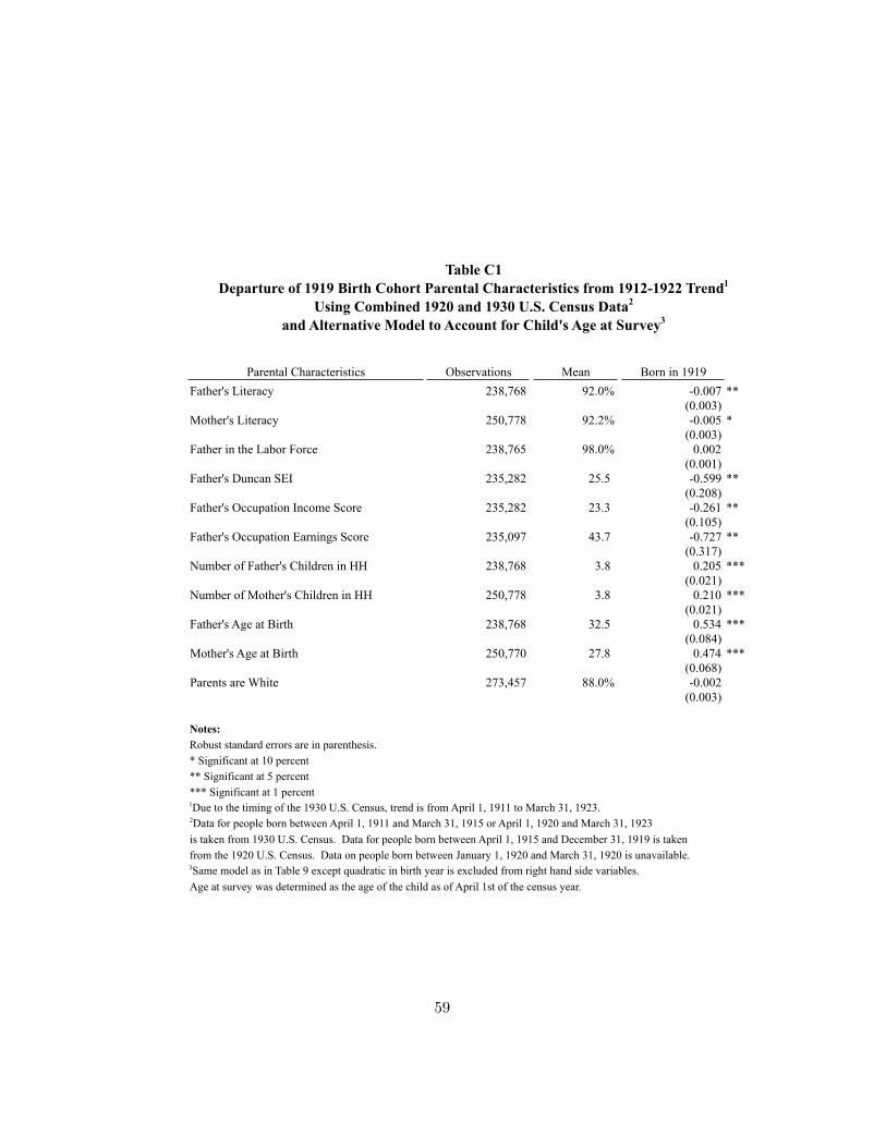
Table C1

Departure of 1919 Birth Cohort Parental Characteristics from 1912-1922 Trend1

Using Combined 1920 and 1930 U.S. Census Data2

and Alternative Model to Account for Child's Age at Survey3

Parental Characteristics Observations Mean Born in 1919

Father's Literacy d_litpN 238,768 blitpr 92.0% blitpr -0.007 ** blitprblitpr2

plitpr plitpr (0.003) plitprplitpr2

Mother's Literacy d_litmN 250,778 blitmr 92.2% blitmr -0.005 * blitmrblitmr2

plitmr plitmr (0.003) plitmrplitmr2

Father in the Labor Force d_labfN 238,765 blabfr 98.0% blabfr 0.002 blabfrblabfr2

plabfr plabfr (0.001) plabfrplabfr2

Father's Duncan SEI seiN 235,282 bsei 25.5 burbanp -0.599 ** burbanpbsei2

psei purbanp (0.208) purbanppsei2

Father's Occupation Income Score occN 235,282 bocc 23.3 bwhiter -0.261 ** bocc2

pocc pwhiter (0.105) pocc2

Father's Occupation Earnings Score erscN 235,097 bersc 43.7 bwhitep -0.727 ** bersc2

persc pwhitep (0.317) pwhiteppersc2

Number of Father's Children in HH chldpN 238,768 bchldpr 3.8 bwhiter 0.205 *** bchldpr2

pchldpr pwhiter (0.021) pchldpr2

Number of Mother's Children in HH chldmN 250,778 bchldmr 3.8 bwhitep 0.210 *** bchldmr2

pchldmr pwhitep (0.021) pwhiteppchldmr2

Father's Age at Birth aabpN 238,768 baabpp 32.5 baabp 0.534 *** baabpbaabp2

paabpp paabp (0.084) paabppaabp2

Mother's Age at Birth aabmN 250,770 baabm 27.8 baabm 0.474 *** baabmbaabm2

paabm paabm (0.068) paabmpaabm2

Parents are White d_whiteN 273,457 bwhiter 88.0% bwhiter -0.002 bwhiter

pwhiter pwhiter (0.003) pwhiter

Notes:

Robust standard errors are in parenthesis.

* Significant at 10 percent

** Significant at 5 percent

*** Significant at 1 percent1Due to the timing of the 1930 U.S. Census, trend is from April 1, 1911 to March 31, 1923.2Data for people born between April 1, 1911 and March 31, 1915 or April 1, 1920 and March 31, 1923

is taken from 1930 U.S. Census. Data for people born between April 1, 1915 and December 31, 1919 is taken

from the 1920 U.S. Census. Data on people born between January 1, 1920 and March 31, 1920 is unavailable.3Same model as in Table 9 except quadratic in birth year is excluded from right hand side variables.

Age at survey was determined as the age of the child as of April 1st of the census year.

59

Table C2

Departure of 1919 Birth Cohort Parental Characteristics from 1913-1922 Trend1

Using Combined 1920 and 1930 U.S. Census Data2

and Alternative Model to Account for Child's Age at Survey3

Parental Characteristics Observations Mean Born in 1919

Father's Literacy d_litpN 223,528 blitpr 92.0% blitpr -0.007 ** blitpr2

plitpr plitpr (0.003) plitpr2

Mother's Literacy d_litmN 234,030 blitmr 92.2% blitmr -0.005 blitmr2

plitmr plitmr (0.003) plitmr2

Father in the Labor Force d_labfN 223,525 blabfr 98.1% blabfr 0.001 blabfr2

plabfr plabfr (0.001) plabfr2

Father's Duncan SEI seiN 220,515 bsei 25.4 burbanp -0.512 ** bsei2

psei purbanp (0.210) psei2

Father's Occupation Income Score occN 220,515 bocc 23.2 bwhiter -0.215 ** bocc2

pocc pwhiter (0.107) pocc2

Father's Occupation Earnings Score erscN 220,338 bersc 43.6 bwhitep -0.579 * bersc2

persc pwhitep (0.321) persc2

Number of Father's Children in HH chldpN 223,528 bchldpr 3.8 bwhiter 0.208 *** bchldpr2

pchldpr pwhiter (0.021) pchldpr2

Number of Mother's Children in HH chldmN 234,030 bchldmr 3.7 bwhitep 0.208 *** bchldmr2

pchldmr pwhitep (0.021) pchldmr2

Father's Age at Birth aabpN 223,528 baabpp 32.5 baabp 0.553 *** baabp2

paabpp paabp (0.085) paabp2

Mother's Age at Birth aabmN 234,027 baabm 27.8 baabm 0.514 *** baabm2

paabm paabm (0.069) paabm2

Parents are White d_whiteN 251,056 bwhiter 88.1% bwhiter -0.005 bwhiter

pwhiter pwhiter (0.003) pwhiter

Notes:

Robust standard errors are in parenthesis.

* Significant at 10 percent

** Significant at 5 percent

*** Significant at 1 percent1Due to the timing of the 1930 U.S. Census, trend is from April 1, 1912 to March 31, 1923.2Data for people born between April 1, 1912 and March 31, 1915 or April 1, 1920 and March 31, 1923

is taken from 1930 U.S. Census. Data for people born between April 1, 1915 and December 31, 1919 is taken

from the 1920 U.S. Census. Data on people born between January 1, 1920 and March 31, 1920 is unavailable.3Same model as in Table 10 except quadratic in birth year is excluded from right hand side variables.

Age at survey was determined as the age of the child as of April 1st of the census year.

60

Table C3

Departure of 1919 Male Birth Cohort Parental Characteristics from 1912-1922 Male Trend1

Using Combined 1920 and 1930 U.S. Census Data2

and Alternative Model to Account for Child's Age at Survey3

Parental Characteristics Observations Mean Born in 1919

Father's Literacy d_litpN 122,612 blitpr 92.1% blitpr -0.009 ** blitpr2

plitpr plitpr (0.004) plitpr2

Mother's Literacy d_litmN 128,561 blitmr 92.3% blitmr -0.008 * blitmr2

plitmr plitmr (0.004) plitmr2

Father in the Labor Force d_labfN 122,611 blabfr 98.0% blabfr 0.001 blabfr2

plabfr plabfr (0.002) plabfr2

Father's Duncan SEI seiN 120,866 bsei 25.4 burbanp -0.774 ** bsei2

psei purbanp (0.291) psei2

Father's Occupation Income Score occN 120,866 bocc 23.2 bwhiter -0.320 ** bocc2

pocc pwhiter (0.147) pocc2

Father's Occupation Earnings Score erscN 120,777 bersc 43.6 bwhitep -0.961 ** bersc2

persc pwhitep (0.444) persc2

Number of Father's Children in HH chldpN 122,612 bchldpr 3.8 bwhiter 0.213 *** bchldpr2

pchldpr pwhiter (0.030) pchldpr2

Number of Mother's Children in HH chldmN 128,561 bchldmr 3.8 bwhitep 0.216 *** bchldmr2

pchldmr pwhitep (0.029) pchldmr2

Father's Age at Birth aabpN 122,612 baabpp 32.4 baabp 0.539 *** baabp2

paabpp paabp (0.117) paabp2

Mother's Age at Birth aabmN 128,558 baabm 27.8 baabm 0.490 *** baabm2

paabm paabm (0.095) paabm2

Parents are White d_whiteN 138,575 bwhiter 88.3% bwhiter -0.006 bwhiter

pwhiter pwhiter (0.004) pwhiter

Notes:

Robust standard errors are in parenthesis.

* Significant at 10 percent

** Significant at 5 percent

*** Significant at 1 percent1Due to the timing of the 1930 U.S. Census, trend is from April 1, 1911 to March 31, 1923.2Data for people born between April 1, 1911 and March 31, 1915 or April 1, 1920 and March 31, 1923

is taken from 1930 U.S. Census. Data for people born between April 1, 1915 and December 31, 1919 is taken

from the 1920 U.S. Census. Data on people born between January 1, 1920 and March 31, 1920 is unavailable.3Same model as in Table 11 except quadratic in birth year is excluded from right hand side variables.

Age at survey was determined as the age of the child as of April 1st of the census year.

61

Table C4

Departure of 1919 Birth Cohort Parental Characteristics from 1912-1922 Trend1

Using Combined 1920 and 1930 U.S. Census Data2

and Alternative Model to Account for Child's Age at Survey3

Parental Characteristics Observations Mean Born in 1919

Father's Literacy d_litpN 238,768 blitpr 92.0% blitpr -0.007 ** blitpr2

plitpr plitpr (0.003) plitpr2

Mother's Literacy d_litmN 250,778 blitmr 92.2% blitmr -0.005 * blitmr2

plitmr plitmr (0.003) plitmr2

Father in the Labor Force d_labfN 238,765 blabfr 98.0% blabfr 0.001 blabfr2

plabfr plabfr (0.001) plabfr2

Father's Duncan SEI seiN 235,282 bsei 25.5 burbanp -0.561 ** bsei2

psei purbanp (0.216) psei2

Father's Occupation Income Score occN 235,282 bocc 23.3 bwhiter -0.241 ** bocc2

pocc pwhiter (0.110) pocc2

Father's Occupation Earnings Score erscN 235,097 bersc 43.7 bwhitep -0.667 ** bersc2

persc pwhitep (0.330) persc2

Number of Father's Children in HH chldpN 238,768 bchldpr 3.8 bwhiter 0.239 *** bchldpr2

pchldpr pwhiter (0.022) pchldpr2

Number of Mother's Children in HH chldmN 250,778 bchldmr 3.8 bwhitep 0.241 *** bchldmr2

pchldmr pwhitep (0.022) pchldmr2

Father's Age at Birth aabpN 238,768 baabpp 32.5 baabp 0.593 *** baabp2

paabpp paabp (0.087) paabp2

Mother's Age at Birth aabmN 250,770 baabm 27.8 baabm 0.525 *** baabm2

paabm paabm (0.071) paabm2

Parents are White d_whiteN 273,457 bwhiter 88.0% bwhiter -0.005 bwhiter

pwhiter pwhiter (0.003) pwhiter

Notes:

Robust standard errors are in parenthesis.

* Significant at 10 percent

** Significant at 5 percent

*** Significant at 1 percent1Due to the timing of the 1930 U.S. Census, trend is from April 1, 1911 to March 31, 1923.2Data for people born between April 1, 1911 and March 31, 1915 or April 1, 1920 and March 31, 1923

is taken from 1930 U.S. Census. Data for people born between April 1, 1915 and December 31, 1919 is taken

from the 1920 U.S. Census. Data on people born between January 1, 1920 and March 31, 1920 is unavailable.3Model uses birth year, birth year squared, 1930 census year dummy, 1930 census year dummy interacted with

age at survey, and 1919 birth cohort dummy as right hand side variables.

Age at survey was determined as the age of the child as of April 1st of the census year.

62

Table C5

Departure of 1919 Birth Cohort Parental Characteristics from 1912-1922 Trend1

Using Combined 1920 and 1930 U.S. Census Data2

and Alternative Model to Account for Child's Age at Survey3

Parental Characteristics Observations Mean Born in 1919

Father's Literacy d_litpN 238,768 blitpr 92.0% blitpr -0.007 ** blitpr2

plitpr plitpr (0.003) plitpr2

Mother's Literacy d_litmN 250,778 blitmr 92.2% blitmr -0.005 * blitmr2

plitmr plitmr (0.003) plitmr2

Father in the Labor Force d_labfN 238,765 blabfr 98.0% blabfr 0.001 blabfr2

plabfr plabfr (0.001) plabfr2

Father's Duncan SEI seiN 235,282 bsei 25.5 burbanp -0.561 ** bsei2

psei purbanp (0.216) psei2

Father's Occupation Income Score occN 235,282 bocc 23.3 bwhiter -0.241 ** bocc2

pocc pwhiter (0.110) pocc2

Father's Occupation Earnings Score erscN 235,097 bersc 43.7 bwhitep -0.667 ** bersc2

persc pwhitep (0.330) persc2

Number of Father's Children in HH chldpN 238,768 bchldpr 3.8 bwhiter 0.239 *** bchldpr2

pchldpr pwhiter (0.022) pchldpr2

Number of Mother's Children in HH chldmN 250,778 bchldmr 3.8 bwhitep 0.241 *** bchldmr2

pchldmr pwhitep (0.022) pchldmr2

Father's Age at Birth aabpN 238,768 baabpp 32.5 baabp 0.593 *** baabp2

paabpp paabp (0.087) paabp2

Mother's Age at Birth aabmN 250,770 baabm 27.8 baabm 0.525 *** baabm2

paabm paabm (0.071) paabm2

Parents are White d_whiteN 273,457 bwhiter 88.0% bwhiter -0.005 bwhiter

pwhiter pwhiter (0.003) pwhiter

Notes:

Robust standard errors are in parenthesis.

* Significant at 10 percent

** Significant at 5 percent

*** Significant at 1 percent1Due to the timing of the 1930 U.S. Census, trend is from April 1, 1911 to March 31, 1923.2Data for people born between April 1, 1911 and March 31, 1915 or April 1, 1920 and March 31, 1923

is taken from 1930 U.S. Census. Data for people born between April 1, 1915 and December 31, 1919 is taken

from the 1920 U.S. Census. Data on people born between January 1, 1920 and March 31, 1920 is unavailable.3Model uses birth year, birth year squared, age at survey, age at survey squared, and 1919 birth cohort dummy

as right hand side variables. Age at survey was determined as the age of the child as of April 1st of the census year.

63

Table C6

Departure of 1919 Birth Cohort Parental Characteristics from 1912-1922 Trend1

Using Combined 1920 and 1930 U.S. Census Data2

and Alternative Model to Account for Child's Age at Survey3

Parental Characteristics Observations Mean Born in 1919

Father's Literacy d_litpN 238,768 blitpr 92.0% blitpr -0.007 ** blitpr2

plitpr plitpr (0.003) plitpr2

Mother's Literacy d_litmN 250,778 blitmr 92.2% blitmr -0.006 * blitmr2

plitmr plitmr (0.003) plitmr2

Father in the Labor Force d_labfN 238,765 blabfr 98.0% blabfr 0.002 * blabfr2

plabfr plabfr (0.001) plabfr2

Father's Duncan SEI seiN 235,282 bsei 25.5 burbanp -0.621 ** bsei2

psei purbanp (0.212) psei2

Father's Occupation Income Score occN 235,282 bocc 23.3 bwhiter -0.267 ** bocc2

pocc pwhiter (0.108) pocc2

Father's Occupation Earnings Score erscN 235,097 bersc 43.7 bwhitep -0.748 ** bersc2

persc pwhitep (0.324) persc2

Number of Father's Children in HH chldpN 238,768 bchldpr 3.8 bwhiter 0.217 *** bchldpr2

pchldpr pwhiter (0.022) pchldpr2

Number of Mother's Children in HH chldmN 250,778 bchldmr 3.8 bwhitep 0.222 *** bchldmr2

pchldmr pwhitep (0.021) pchldmr2

Father's Age at Birth aabpN 238,768 baabpp 32.5 baabp 0.529 *** baabp2

paabpp paabp (0.085) paabp2

Mother's Age at Birth aabmN 250,770 baabm 27.8 baabm 0.468 *** baabm2

paabm paabm (0.070) paabm2

Parents are White d_whiteN 273,457 bwhiter 88.0% bwhiter 0.000 bwhiter

pwhiter pwhiter (0.003) pwhiter

Notes:

Robust standard errors are in parenthesis.

* Significant at 10 percent

** Significant at 5 percent

*** Significant at 1 percent1Due to the timing of the 1930 U.S. Census, trend is from April 1, 1911 to March 31, 1923.2Data for people born between April 1, 1911 and March 31, 1915 or April 1, 1920 and March 31, 1923

is taken from 1930 U.S. Census. Data for people born between April 1, 1915 and December 31, 1919 is taken

from the 1920 U.S. Census. Data on people born between January 1, 1920 and March 31, 1920 is unavailable.3Model uses age at survey, age at survey squared, 1930 census year dummy, and 1919 birth cohort dummy

as right hand side variables. Age at survey was determined as the age of the child as of April 1st of the census year.

64

Departure of 1918 Birth Cohort Parental Characteristics from 1912-1922 Trend1

Using Combined 1920 and 1930 U.S. Census Data2

and Model to Account for Child's Age at Survey3

Parental Characteristics Observations Mean Born in 1918

Father's Literacy d_litpN 238,768 blitpr 92.0% blitpr 0.007 ** blitpr2

plitpr plitpr (0.002) plitpr2

Mother's Literacy d_litmN 250,778 blitmr 92.2% blitmr 0.009 *** blitmr2

plitmr plitmr (0.002) plitmr2

Father in the Labor Force d_labfN 238,765 blabfr 98.0% blabfr 0.000 blabfr2

plabfr plabfr (0.001) plabfr2

Father's Duncan SEI seiN 235,282 bsei 25.5 burbanp 0.630 *** bsei2

psei purbanp (0.165) psei2

Father's Occupation Income Score occN 235,282 bocc 23.3 bwhiter 0.348 *** bocc2

pocc pwhiter (0.084) pocc2

Father's Occupation Earnings Score erscN 235,097 bersc 43.7 bwhitep 0.992 *** bersc2

persc pwhitep (0.252) persc2

Number of Father's Children in HH chldpN 238,768 bchldpr 3.8 bwhiter -0.194 *** bchldpr2

pchldpr pwhiter (0.017) pchldpr2

Number of Mother's Children in HH chldmN 250,778 bchldmr 3.8 bwhitep -0.198 *** bchldmr2

pchldmr pwhitep (0.016) pchldmr2

Father's Age at Birth aabpN 238,768 baabpp 32.5 baabp -0.230 *** baabp2

paabpp paabp (0.066) paabp2

Mother's Age at Birth aabmN 250,770 baabm 27.8 baabm -0.201 *** baabm2

paabm paabm (0.054) paabm2

Parents are White d_whiteN 273,457 bwhiter 88.0% bwhiter 0.010 *** bwhiter

pwhiter pwhiter (0.002) pwhiter

Notes:

Robust standard errors are in parenthesis.

* Significant at 10 percent

** Significant at 5 percent

*** Significant at 1 percent1Due to the timing of the 1930 U.S. Census, trend is from April 1, 1911 to March 31, 1923.2Data for people born between April 1, 1911 and March 31, 1915 or April 1, 1920 and March 31, 1923

is taken from 1930 U.S. Census. Data for people born between April 1, 1915 and December 31, 1919 is taken

from the 1920 U.S. Census. Data on people born between January 1, 1920 and March 31, 1920 is unavailable.3Model uses birth year, birth year squared, 1930 census year dummy, 1930 census year dummy interacted with

quadratic in age at survey, and 1918 birth cohort dummy as right hand side variables.

Age at survey was determined as the age of the child as of April 1st of the census year.

Table C7

65

Departure of 1920 Birth Cohort Parental Characteristics from 1912-1922 Trend1,2

Using Combined 1920 and 1930 U.S. Census Data3

and Model to Account for Child's Age at Survey4

Parental Characteristics Observations Mean Born in 19201

Father's Literacy d_litpN 238,768 blitpr 92.0% blitpr 0.001 blitpr2

plitpr plitpr (0.002) plitpr2

Mother's Literacy d_litmN 250,778 blitmr 92.2% blitmr 0.004 * blitmr2

plitmr plitmr (0.002) plitmr2

Father in the Labor Force d_labfN 238,765 blabfr 98.0% blabfr 0.001 blabfr2

plabfr plabfr (0.001) plabfr2

Father's Duncan SEI seiN 235,282 bsei 25.5 burbanp 0.203 bsei2

psei purbanp (0.186) psei2

Father's Occupation Income Score occN 235,282 bocc 23.3 bwhiter 0.124 bocc2

pocc pwhiter (0.091) pocc2

Father's Occupation Earnings Score erscN 235,097 bersc 43.7 bwhitep 0.437 bersc2

persc pwhitep (0.268) persc2

Number of Father's Children in HH chldpN 238,768 bchldpr 3.8 bwhiter -0.042 ** bchldpr2

pchldpr pwhiter (0.018) pchldpr2

Number of Mother's Children in HH chldmN 250,778 bchldmr 3.8 bwhitep -0.050 ** bchldmr2

pchldmr pwhitep (0.018) pchldmr2

Father's Age at Birth aabpN 238,768 baabpp 32.5 baabp -0.127 * baabp2

paabpp paabp (0.068) paabp2

Mother's Age at Birth aabmN 250,770 baabm 27.8 baabm 0.028 baabm2

paabm paabm (0.058) paabm2

Parents are White d_whiteN 273,457 bwhiter 88.0% bwhiter -0.004 bwhiter

pwhiter pwhiter (0.003) pwhiter

Notes:

Robust standard errors are in parenthesis.

* Significant at 10 percent

** Significant at 5 percent

*** Significant at 1 percent1Due to the timing of the 1930 U.S. Census, 1920 birth cohort consists of people born between

April 1, 1920 and March 31, 1921.2Due to the timing of the 1930 U.S. Census, trend is from April 1, 1911 to March 31, 1923.3Data for people born between April 1, 1911 and March 31, 1915 or April 1, 1920 and March 31, 1923

is taken from 1930 U.S. Census. Data for people born between April 1, 1915 and December 31, 1919 is taken

from the 1920 U.S. Census. Data on people born between January 1, 1920 and March 31, 1920 is unavailable.4Model uses birth year, birth year squared, 1930 census year dummy, 1930 census year dummy interacted with

quadratic in age at survey, and 1920 birth cohort dummy as right hand side variables.

Age at survey was determined as the age of the child as of April 1st of the census year.

Table C8

66