Embed Size (px)
Citation preview

The 2008 U.S. Auto Market Collapse∗
Bill Dupor†, Rong Li‡, Saif Mehkari§, and Yi-Chan Tsai¶
October 4, 2018
Abstract
New vehicle sales in the U.S. fell nearly 40 percent during the last recession, causing signif-icant job losses and unprecedented government interventions in the auto industry. This paperexplores two potential explanations for this decline: falling home values and falling households’income expectations. First, we establish that declining home values explain only a small portionof the observed reduction in household new vehicle sales. Using a county-level panel from theepisode, we find: (1) A one-dollar fall in home values reduced household new vehicle spendingby 0.5 to 0.7 cents and overall new vehicle spending by 0.9 to 1.2 cents; and (2) Falling homevalues explain between 16 and 19 percent of the overall new vehicle spending decline. Next,examining state-level data from 1997-2016, we find: (3) The short-run responses of new vehicleconsumption to home value changes are larger in the 2005-2011 period relative to other years,but at longer horizons (e.g. 5 years), the responses are similar across the two sub-periods; and(4) The service flow from vehicles, as measured by miles traveled, responds very little to houseprice shocks. We also detail the sources of the differences between our findings (1) and (2)from existing research. Second, we establish that declining current and expected future incomeexpectations potentially played an important role in the auto market’s collapse. We build apermanent income model augmented to include infrequent, repeated car buying. Our calibratedmodel matches the pre-recession distribution of auto vintages and the liquid-wealth-to-incomeratio, and exhibits a large vehicle sales decline in response to a mild decline in expected per-manent income due to a transitory slowdown in income growth. In response to the shock,households delay replacing existing vehicles, allowing them to smooth the effects of the incomeshock without significantly adjusting the service flow from their vehicles. Combining our neg-ative results regarding housing wealth with our positive model-based findings, we interpret theauto market collapse as consistent with existing permanent income based approaches to durablegoods purchases (e.g., Leahy and Zeira (2005)).
∗Thanks to Evan Carson, James Eubanks and Rodrigo Guerrero for useful research assistance as well as Adrienne Brennecke
for help acquiring the auto count data. The analysis set forth does not reflect the views of the Federal Reserve Bank of St.
Louis or the Federal Reserve System. We thank John Leahy for very useful comments.† Federal Reserve Bank of St. Louis, [email protected], [email protected].‡ School of Finance, Renmin University of China, [email protected].§ University of Richmond, [email protected].¶ National Taiwan University, [email protected].
1

1 Introdution
The decline in autos purchased played a large role in the personal consumption decline during the
last recession. Figure 1 plots the accumulated change in motor vehicle consumption relative to
2007.1 It drops dramatically, reaching negative $200 billion by 2010, and recovers very slowly. In
contrast, as seen in the figure, the corresponding variable for total consumption (excluding vehicles)
never becomes negative and recovers very quickly.
Figure 1: Cumulative change in components of personal consumption expenditure since 2007
-200
0
200
400
600
800
Bill
ions
of D
olla
rs
2008 2009 2010 2011
Motor vehicle consumptionTotal consumption net of motor vehicle consumption
Notes: Data are annual and from the Bureau of Economic Analysis. Each bar corresponds to the accumulated change
in Xt measured as∑δt=2008 (Xt −X2007).
The new vehicle sales decline was intense and violent. In one 12-month period alone, personal
new vehicle sales fell by $107 billion.2 By Spring of 2009, Chrysler and General Motors faced
bankruptcy. This led the U.S. government to use TARP funds to bailout both. At one point, the
1Our usage of the phrase motor vehicle consumption here follows BEA terminology. Later in the paper, weassociate investment in the stock of durables with consumption and distinguish it from the consumption of theservice flow from the stock of vehicles in the economy.
2This is a nominal seasonally-adjusted rate between 2007Q4 and 2008Q4.
2

federal government owned 61 percent of General Motors.3
Despite the bailout, the decline in new vehicle sales had a devastating impact. Over a 2-year
period, employment in the motor vehicle industry fell over 45 percent, which excludes additional
knock-on effects reverberating through upstream and downstream industries.
The story is not a new one. As Martin Zimmerman (1998), then-chief economist at Ford Motor
Company, wrote “I cannot think of an industry more cyclical or more dependent on the business
cycle than the auto industry.”
This paper explores two potential explanations for the auto market collapse: falling home values
and changes in income expectations. We begin with the housing market. One view holds that, as
homeowners see house prices fall, they internalize this as a reduction in wealth and respond by cut-
ting auto purchases. This effect might be stronger if homeowners use home equity to purchase cars.
With falling house prices, homeowners become more borrowing constrained which only intensifies
the fall in auto sales.
In the first part of this paper, we exploit variation in home value and price changes to assess
the role of home prices in explaining the auto sales collapse. We regress new auto sales on home
values across U.S. counties and show that a one dollar decline in home values reduced household
new auto spending by between 0.5 and 0.7 cents. Overall new auto spending, i.e., from consumers,
businesses and government, fell by between 0.9 and 1.2 cents in response to the same change. This
relatively weak response helps explain our second finding: falling home values explain between 16
and 19 percent of the overall new auto sales reduction during the period.4 In the historic auto
market collapse, declining home values played a small part.5
The relatively mild responses of auto sales to home value changes might seem surprising given
the attention researchers have placed on household leverage during the period. Aggregate household
debt-to-income rose from roughly 0.75 in 1997 to its peak of 1.2 in 2009. According to one view,
over-levered households should have dramatically cut back auto purchases because of their falling
housing wealth.
If leverage effects were quantitatively important in the aggregate during the last recession, then
one might expect to see even smaller responses of auto sales to home values outside of that period.
We test this possibility by estimating similar responses using a panel of annual state-level data
from 1997-2017. The state-level data are based on the same underlying house prices but we replace
vehicle sales counts with BEA motor vehicle consumption data.
Our state-level estimates of the response elasticities of motor vehicle consumption to house price
3“GM and Chrysler, owned by the government, lobby the government,” The Washington Post, January 13, 2011.4Later in the paper, we compare our findings to those of MRS (2013), who run similar regressions and report a
much larger response of auto sales to home values.5Our paper, like many others studying macroeconomic phenomenon using cross-sectional regressions, suffers from
the potential complication associated with estimating relative rather than aggregate effects of shocks or policy changes.Nakamura and Steinsson (2014), Dupor and Guerrero (2017) and Dupor and Guerrero (2018) present discussions andsuggest strategies for comparing aggregate and relative effects in the context of fiscal multipliers.
3

changes are broadly in line with our results described above. There is a positive and statistically
significant, but quantitatively mild, effect of house prices. The short-run responses (i.e. 1 to 3-
years) are somewhat larger; however, at longer horizons (e.g., 5-years) leverage has little effect on
the causal impact of home values on vehicle sales.
Next, we examine the effect of home values on auto usage. We replace auto sales with vehicle
miles travelled in our state-level regressions and show that miles travelled was nearly unaffected
by changes in home values. As such, households were able to smooth the flow of services from
the stock of vehicles, as measured by miles traveled, in response to house price shocks. From the
households’ perspective, home price shocks did not disrupt auto usage.
Having established that house prices played a minor role in explaining the auto sales collapse,
the natural question is: what caused the auto sales decline? According to the PIH, households
will reduce current consumption when expected future income falls, even in absence of borrowing
constraints or reductions in tangible wealth. Moreover, if the expected future income declines were
broad-based, it may be difficult to identify this effect using astructural cross-sectional regressions.
We provide microeconomic survey evidence showing that many individuals decided it was a
bad time to purchase a car; moreover, the surveys establish that poor current and expected future
economic conditions were primary drivers of this increased aversion to auto buying.
These survey-based findings motivate an alternative explanation for the auto market’s collapse:
falling future income expectations.6
The durability of autos together with the discrete nature with which individuals adjust their
auto stocks may be important. During the last recession, households may have cut back on new
auto purchases and simultaneously maintained their driving patterns by continuing to use their
existing autos for a period of time.
With this in mind, we build a model with nondurable consumption, savings and infrequent,
repeated auto purchases. In the model, individuals are subject to transitory idiosyncratic level
income shocks and an unanticipated persistent aggregate income growth rate shock. The latter
shock is calibrated to drive a mild decline in expected permanent income. Individuals optimally
respond to negative shocks of this kind by delaying auto replacement. The model matches the cross
sectional distribution of autos by vintages and liquid-wealth-to-income ratio in the period prior to
the 2007-2009 recession.
The shock amplification mechanism is very strong: a 3.1 percent decline in expected permanent
income drives a 45 percent decline in aggregate new vehicle sales.
Our paper relates to several lines of research. McCully, Pence and Vine (2015) report that
very few households in the U.S. purchase cars with home equity lines or credit or proceeds from
6This brings to mind De Nardi, French and Benson (2012), who study how large a decline in future income wouldbe required to explain the observed fall in total real personal expenditures based on a permanent income model. Thatpaper finds that a large persistent decline in expected future income is capable of causing the decline in aggregateconsumption. De Nardi, French and Benson (2012) use a model with only nondurable consumption to perform theircalculations.
4

cash-out refinancing. Auto buyers that do use these sources are affluent and have ample access to
credit. Along the same lines, it is somewhat incongruous to think about borrowing constraints as
important for an acquiring autos, since a purchased auto is itself collateral for its corresponding
auto loan.
Other papers link the home price decline during the last recession to the drop in consumer
spending in the U.S. These include Mian, Rao and Sufi (2013), which finds a strong positive
relationship between house prices and both durable and nondurable consumption during the period.
Based on county-level data, MRS report that consumption increases by 5.4 cents from a one dollar
increase in housing wealth. They find that 43 percent of this increase (2.3 cents per dollar) comes
from new auto spending. We explain the reasons for differences between our findings and MRS and
detail several pitfalls with their approach later in the paper.
Kaplan, Mitman and Violante (2016) find a positive relationship between house prices and
nondurable consumption in the cross section during the last recession. General equilibrium analyses
regarding consumption and the housing market include Garriga and Hedlund (2017) and Kaplan,
Mitman and Violante (2017). Most of the papers on the consumption response to house value
changes focus on non-durable consumption. They do not model non-housing durable goods, we do
in our paper.7 Lehnert (2004) is a seminal early contribution on the consumption effects of home
value changes.
Our economic model’s mechanism has been described in existing theoretical work. Leahy and
Zeira (2005) present a model with infrequent durable goods purchases in which the timing decision
of auto purchases amplifies and propagates shocks. In response to negative shocks, individuals who
were going to purchase the durable good postpone their purchases.8
There are other–at least partial–explanations for the auto sales collapse. Benmelech, Meisenzahl
and Ramcharan (2017) argue that the disruption in the asset-backed commercial paper market
reduced the availability of auto loans, and caused up to 31 percent of the auto sales fall during the
episode. Another explanation focuses on the mismatch between the increased demand for higher
efficiency cars, in light of positive oil price shocks, with the lack of supply of efficient vehicles by
some major auto manufacturers.
Section 2 presents our county-level findings from the 2007-2009 Recession. Section 3 presents
our state-level findings using data from the past two decades. It finds a weak response of auto sales,
and also miles traveled, to home value changes. Section 4 presents a dynamic permanent income
model augmented with auto purchases in which declines in expected permanent income generate
large decline in aggregate autos purchased. The final section recaps.
7These include, for example, Berger, et.al. (2018), Corbae and Quintin (2015), and Favilukis, Ludvigson and VanNieuwerburg (2016).
8Empirical work on autos and the permanent income hypothesis include Adda and Cooper (2000), Bernanke (1984)and Eberly (1994).
5

2 County-Level Analysis
2.1 Data and Econometric Model
Let Ai,t denote the dollar value of new vehicles sold overall in county i in quarter t. We calculate auto
counts from county-level auto registrations, which includes vehicles sold to households, businesses
and government.9 The vehicles acquired include those gotten via: straight cash purchases, trade-in
purchases, leases, etc. To go from quantities to dollar values, we multiply the quantity of autos
by the nationwide average new auto price, which was in a range of $26,200 to $26,950 during the
period according to the Bureau of Transportation Statistics.10
At times we distinguish the household response of vehicle spending from that of overall vehicle
spending. We map from overall spending to household spending by using the aggregate share of new
vehicles purchased by consumers as a fraction of total new vehicle purchases (from consumers, busi-
nesses and government), which is available annually from the Bureau of Transportation Statistics.
Over 40 percent of new cars are sold to businesses and government during this period.11
Let Vi,t denote the dollar value of the owner-occupied housing stock in county i in quarter t.
CoreLogic constructs monthly house price data at the county-level; however, these are reported as
indices rather than dollar amounts. To go from indices to dollar prices, we begin with the county-
level median house price available from the 2000 U.S. Census. Then we multiply this Census house
price by the gross growth rate of the Corelogic index between the month of interest and January
of 2000. Let Pi,t denote the current dollar price of an owner-occupied house, calculated according
to the procedure.
To calculate the value of the county-level housing stock we multiply Pi,t by the number of
households in owner-occupied housing from the 2006 Census.
Let ai,t,δ = log (Ai,t+δ−1) − log (Ai,t−1). Next, let aci,t,δ be the cumulative percentage increase
in auto sales over a δ quarter horizon relative to a quarter t− 1 baseline in county i:
aci,t,δ =1
4
δ∑j=1
ai,t,j
The variables pi,t,δ and pci,t,δ are defined similarly.12
Let pi,t,δ and pci,t,δ denote the nation-wide averages of their county-level counterparts, where the
9Vehicles includes autos, light trucks and SUV.10Average new car auto prices changed very little during the period considered. The federal data on auto price
stops in 2010, and we use the 2010 price for later years where required. See Table 11 in the Appendix for the timeseries of the average new vehicle price over this period.
11See Table 12 in the Appendix for the time series on the share of new autos purchased by households.12The use of accumulated growth rates means that our resulting regression coefficients can be interpreted as areas
under impulse response functions. Ramey and Zubairy (2017) argue compellingly that this is an useful way tosummarize dynamic responses to shocks.
6

averages are weighted by the number of households in a county.
Defining these variables as such permits us to estimate the dynamic, cumulative responses of
auto sales to house value shocks. Cumulative responses give the change in auto sales accumulated
over a specific horizon with respect to the accumulated change in home prices over the same
horizon.13
First, we estimate the elasticity of vehicle sales to house price changes, using:
aci,t,δ = φδpci,t,δ + βδXi,t + vi,t,δ (1)
for δ = 1, ..., D. By the form it takes, equation (1) implements the Jorda (2005) local projections
approach.
Here, Xi,t consist of a linear trend, seasonal dummies and a “cash for clunkers” dummy, which
equals one in 2009Q3 through 2010Q1. We also include one lag of the growth rate in auto sales
and house prices at t− 1 (i.e., ai,t−1,1 and pi,t−1,1). The sample covers 2007Q2 through 2010Q2.
The coefficient φδ is then the cumulative percentage increase in auto sales through horizon δ in
response to a 1 percent increase in house prices (cumulative through horizon δ). We shall call this
the dynamic sales elasticity or simply the sales elasticity. The estimation uses least-squares and is
weighted by the number of households in a county. We report heteroskedasticity and autocorrelation
corrected (HAC) standard errors throughout the paper.
Table 1 reports the sales elasticities at various horizons. Note that the largest potential sample
size falls as we move to longer horizons because we lose observations as we extend the horizon of
the cumulative responses. To make estimates more comparable, every estimate is based on the
observations for the 3 year horizon sample.
Column (1) reports a one-year elasticity equals 1.08 (SE=0.059). Columns (2) and (3) report the
2- and 3-year horizon responses. The responses are all positive and statistically different from zero.
Moreover the responses fall with the horizon. The 3-year sales elasticity equal 0.60 (SE=0.03).
Interestingly, the cumulative response of auto sales falls rather than increases in response to an
accumulated change in home prices. In a standard adjustment cost model, if changes the growth
rate of purchases of a good lead to additional convex costs, this would lead to a gradual increasing
cumulative response to a positive wealth shock. On the other hand, the decreasing cumulative
response seen in Table 1 may be due to the durable nature of autos.
A short-run increase in vehicle sales in response to a positive house price shock is not simply
an immediate increase in sales with no related dynamic effects. Rather, an increase in house
prices could in part generate greater sales immediately because the now-richer households pull
consumption from the future to the present.
The control variable coefficients are all statistically different from zero and of the expected
13Later in the paper, we estimate the regressions in growth rates rather that cumulative changes for a specificcross-section. The main findings using either approach are similar.
7

Table 1: Cumulative overall new sales elasticities to home price changes, county-level, least squares)
(1) (2) (3)Coef./SE Coef./SE Coef./SE
1-yr cum HP growth 1.079*** - -(0.059)
2-yr cum HP growth - 0.696*** -(0.041)
3-yr cum HP growth - - 0.599***(0.033)
Vehicles sold (lag -0.001* -0.005*** -0.009***growth rate) (0.001) (0.001) (0.002)House Price (lag 0.005*** 0.011*** 0.016***growth rate) (0.001) (0.003) (0.004)Cash for Clunker FE 0.086*** 0.150*** 0.144***
(0.009) (0.018) (0.028)Quarter 0.006*** 0.066*** 0.140***
(0.001) (0.002) (0.003)
R2 0.39 0.58 0.66N 14916 14916 14916
Notes: The dependent variable is the cumulative percentage change in new auto sales at the appropriate horizon. *
p < .1, ** p < .05, *** p < .01. Regressions weight each observation by the number of households in the county
and include seasonal fixed effects (not reported). Standard errors are robust with respect to heteroskedacity and
autocorrelation. HP = home price.
8

signs. The Cash-for-Clunkers fixed effect coefficient is positive, indicating (very sensibly) that sales
growth was stronger over horizons that included the government incentive program. The coefficient
on lagged house price growth is positive, suggesting a somewhat delayed reaction of vehicle sales
to auto prices. Finally, the coefficient on vehicle sales is negative. This is likely due to the durable
nature of autos. Intuitively, a recent past period of intense accumulation of the stock of autos likely
reduces the need to invest in autos in the near future. The coefficients on the second and third
quarter seasonal dummies, not reported here, are positive and statistically different from zero.
Under a set of simplifying assumptions, one can map an elasticity reported here into a derivative:
specifically, the per dollar change in overall vehicle spending in response to a one dollar increase in
home values. Suppose new auto prices and the home ownership rate are roughly unchanged over the
period. Then this derivative is approximately equal to the corresponding estimated elasticity times
the ratio of the value of new vehicles sold relative to the value of the housing stock, averaged over
the same period. For the 2006-2009 period, this ratio is approximately 0.02. In other words, the
value of the housing stock is about 50 times greater than value of one-year’s overall auto purchases.
This implies that, at the 3-year horizon, each dollar of additional housing wealth increases
overall auto sales by 1.2 cents (= 0.02× 0.599). This is an approximation. In the next subsection,
we estimate this derivative, sometimes called a marginal propensity to consume, directly.
2.2 Vehicle Acquisition Responses
Next, we estimate the model using cumulative changes in levels rather than cumulative changes in
growth rates. All of the variables in this subsection are reported in per household terms. Define
V ci,t,δ =
1
4
δ∑j=1
(Vi,t+δ−1 − Vi,t−1)
and let Aci,t,δ be defined analogously. The regression specification is:
Aci,t,δ = βδVci,t,δ + ΓδSi,t + εi,t
Here, Si,t consist of a linear trend, seasonal dummies and a “cash for clunkers” dummy, which
equals one in the 2009Q3-2010Q1. We also include one lag of the change in auto sales and house
vales at t−1 (i.e., ∆Ai,t−1 and ∆Vi,t−1 and). As before, the regressions are weighted by the number
of households in the county.
This second model has a straightforward interpretation. We call the coefficient βδ the overall
vehicle acquisition response, or acquisition response (AQR). It is the cumulative dollar change in
vehicle acquisitions in a county over a δ quarter horizon in response to a one dollar cumulative
increase in housing values over the same δ quarter horizon.
9

This term more precisely describes what we actually can measure given the data available
than some other language used in existing research, such as the marginal propensity to consume
(MPC). The language MPC is not suitable in the current context. First, vehicles are durable goods;
households and business consume the service flow from their stock of durables. Second, while our
data tell us something about durable goods investment through new car registrations, we do not
know the extent to which individuals disinvested in vehicles by scrapping or selling their existing
stock. An individual who purchases a new car but “trades in” a similar but slightly used car may
experience a very small increase in the flow of services despite the new car purchase.
To this point, Figure 2 plots indices calculated from the number of new autos sold along with the
total vehicle miles travelled during the period. While new auto sales fall dramatically, total vehicle
miles travelled changes very little. This suggests that the flow of services associated with autos was
been nearly unchanged, meaning that households were largely able to smooth consumption of auto
usage.
A slightly better, but also deficient, term might be marginal propensity to spend (MPS). Since
we do not know the frequency or value of trade-ins for new vehicle purchases, we cannot infer how
much out of pocket spending occurred when a vehicle is acquired. Even apart from trade-ins, many
vehicles are rented, or leased. In this case, a person who acquires an auto would spend only a
fraction of the auto’s full purchase price.
Table 2 presents the overall (i.e., inclusive of consumers, businesses and government) AQR at
three different horizons. Examining columns (1) through (3), note that the AQR is positive and
statistically different from zero at each horizon. The response is nearly unchanged across horizons.
We focus particular attention on the 3-year horizon, since a related paper (MRS 2013) examines
3-year changes throughout. The 3-year AQR equals 0.012 (SE=0.001). This means that a one
dollar increase in home values is associated with a 1.2 cent increase in auto sales. Reassuringly, the
estimate of the AQR is equal to the approximated value using the elasticity estimate of the last
section.
Vehicle registrations include those of businesses, governments and consumers. Thus, our overall
AQR reflects the contribution of both types of buyers.
To distinguish the overall AQR from the household AQR, we map from overall spending to
household spending by using the aggregate share of new autos purchased by consumers as a frac-
tion of total new auto purchases (from consumers, businesses and government), which is available
annually from the Bureau of Transportation Statistics. Over 40 percent of new cars are sold to
businesses and government during this period.14
Table 14 presents the household AQR regressions based on this measure of vehicle sales. The
coefficient should be interpreted as the response of vehicles acquired for personal use to a change
14The time series for this share appears in Table 12 in the appendix. This partition implicitly assumes that theshare of vehicles sold to individuals in a county approximates that counties’ share of vehicles sold to both individualsand businesses.
10
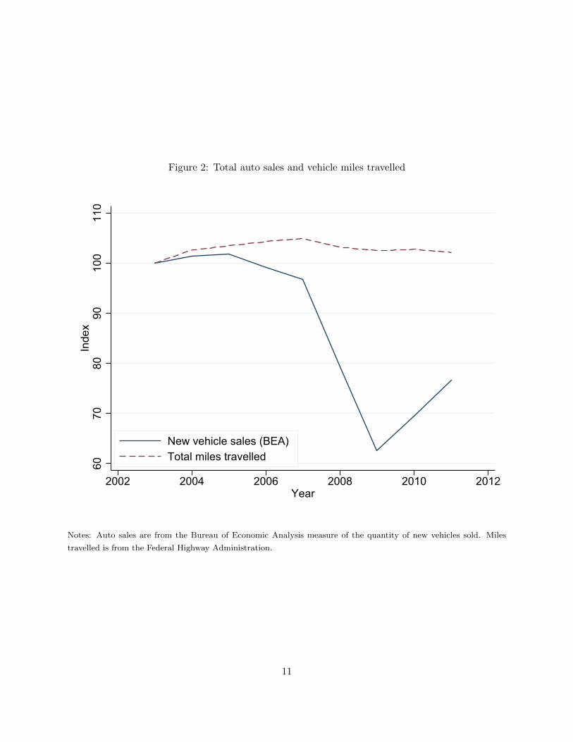
Figure 2: Total auto sales and vehicle miles travelled
6070
8090
100
110
Inde
x
2002 2004 2006 2008 2010 2012Year
New vehicle sales (BEA)Total miles travelled
Notes: Auto sales are from the Bureau of Economic Analysis measure of the quantity of new vehicles sold. Miles
travelled is from the Federal Highway Administration.
11

Table 2: Cumulative overall vehicle acquisition responses, county-level panel
(1) (2) (3)Coef./SE Coef./SE Coef./SE
1-yr Cum Home Val 0.012*** - -Change (0.002)2-yr Cum Home Val - 0.011*** -Change (0.001)3-yr Cum Home Val - - 0.012***Change (0.001)Vehicles sold (lag -0.131 -0.391 -0.628change) (0.244) (0.521) (0.867)House value (lag 0.008 0.014 0.016change) (0.006) (0.013) (0.021)Cash for Clunker FE 0.343*** 0.447* 0.569
(0.110) (0.243) (0.416)Quarter 0.055*** 0.282*** 0.504***
(0.008) (0.018) (0.033)
R2 0.15 0.22 0.22N 13673 13673 13673
Notes: The dependent variable is the cumulative change in vehicle sales at the appropriate horizon. * p < .1, ** p
< .05, *** p < .01. Regressions weight each observation by the number of households in the county and includes
seasonal fixed effects (not reported). Standard errors are robust with respect to heteroskedacity and autocorrelation.
12
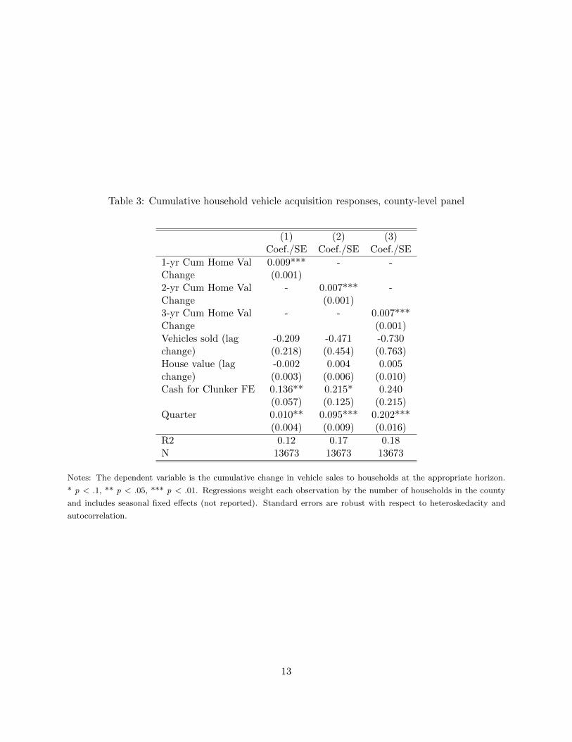
Table 3: Cumulative household vehicle acquisition responses, county-level panel
(1) (2) (3)Coef./SE Coef./SE Coef./SE
1-yr Cum Home Val 0.009*** - -Change (0.001)2-yr Cum Home Val - 0.007*** -Change (0.001)3-yr Cum Home Val - - 0.007***Change (0.001)Vehicles sold (lag -0.209 -0.471 -0.730change) (0.218) (0.454) (0.763)House value (lag -0.002 0.004 0.005change) (0.003) (0.006) (0.010)Cash for Clunker FE 0.136** 0.215* 0.240
(0.057) (0.125) (0.215)Quarter 0.010** 0.095*** 0.202***
(0.004) (0.009) (0.016)
R2 0.12 0.17 0.18N 13673 13673 13673
Notes: The dependent variable is the cumulative change in vehicle sales to households at the appropriate horizon.
* p < .1, ** p < .05, *** p < .01. Regressions weight each observation by the number of households in the county
and includes seasonal fixed effects (not reported). Standard errors are robust with respect to heteroskedacity and
autocorrelation.
13

in home values. The coefficients at the three horizons are between 0.007 and 0.009.
2.3 A Cross-Sectional Specification
In a well-known paper, MRS (2013) also estimate the response of consumer new vehicle sales to
home value changes. They use a cross-section rather than panel analysis and use changes in
home values rather cumulative changes. In their baseline specification, they estimate a coefficient–
analogous to our AQR–equal to 2.3 cents. Thus, their estimate is over 300 percent larger than
ours.
To compare our findings with MRS (2013), we modify our specification to: (a) use a cross-
section, (b) study changes in auto sales and home values, and (c) strip out some of the control
variables used above.
Our dependent variable is the change in the dollar value of overall auto acquisitions between
the first half of 2007 and the first half of 2009 in county j. We choose 2009 as the end year because
it follows the collapse of vehicle sales that began in September of 2008. It excludes the second
half of 2009 because this period contains a transitory spike in sales due to the Cash for Clunkers
program. We choose the starting year as 2007 because it precedes the auto market’s collapse and
also it is the first year of data available to us. Our independent variable is the change in the value
of the housing stock in each county between 2007H1 and 2009H1.
We estimate the cross-sectional model in a way that necessitates fewer control variables than
in our panel regressions. First, we take differences over the same half-years, therefore we do not
require seasonal dummies. Second, the estimation sample ends before implementation of Cash-for-
Clunkers, which eliminates the need for the corresponding fixed effect. We estimate the model with
and without lagged changes in vehicle sales and home values.15
Table 4 contains the first set of regressions. It reports HAC standard errors and uses observation
weights given by the number of households in each county. Column (1) contains the simplest
specification. The coefficient on the change in home values equals 0.010 (SE = 0.002). That is, an
increase in housing value of one dollar in a county is associated with a one cent increase in new
vehicles acquired (by households, businesses and government) in that county. In this specification,
the coefficient equals the AQR. As with the cumulative response, there is a muted, but statistically
significant and precisely estimated, increase in overall auto acquisitions in response to increases in
home values.
Next, the intercept coefficient plays an important role in the study. The intercept coefficient can
be interpreted as the best linear predictor of the change in auto sales in a county with no change in
home values. Its value equals -1.42 (SE = 0.07). The weighted average of the dependent variable
is -1.65. This implies that 80 percent (= -1.42 / -1.65) of the typical new auto sales change in a
county is captured by the intercept rather than being associated with the change in home values.
15MRS (2013) do not include lagged variables in their specifications.
14

The reduction in sales by vehicle manufacturers was nationwide, occurring largely in regions
with and without depressed house prices. There is a small effect of declining home values on vehicle
sales no doubt, but most of the decline in vehicle acquisitions is captured in the regression intercept.
Table 4: Overall vehicle acquisition responses (AQR) of new vehicle sales to changes in home values
(1) (2) (3) (4)Coef./SE Coef./SE Coef./SE Coef./SE
Home value change 0.010*** 0.011*** 0.011*** 0.009***07H1-09H1 (0.002) (0.002) (0.002) (0.002)Home value change - -0.007 -0.008 -0.008*06H1-07H1 (0.005) (0.005) (0.005)Income pc (2006) - - -0.006** -
(0.003)Nonbank finance loan - - - -1.968***share (0.368)Intercept -1.422*** -1.389*** -1.042*** -0.622***
(0.073) (0.078) (0.164) (0.140)Frac. explained by home value declines 0.185 0.209 0.193 0.163
R2 0.114 0.118 0.126 0.156N 1243 1243 1242 1243
Notes: The dependent variable is the change in auto sales (annualized, 000s dollars per household). * p < .1, ** p <
.05, *** p < .01. “Fraction explained by home value declines” is the proportion of the average change in auto sales
due to falling home values. Changes in variables are computed from 2007H1 to 2009H1. Regressions weight each
observation by the number of households in the county. hh=household.
To a great extent, new auto sales fell because the average household and business in most
counties cut back on auto purchases, and not because of declining sales of the average car owner
mainly in counties that experienced dramatic house price declines.
One can also see the limited role of housing in explaining the auto market collapse by applying
the following counterfactual to our regression results. Take the vector of observations of house value
changes in the sample and change every negative value to instead equal zero. Next, compute the
fitted values from the regression using the non-negative modified vector. These fitted values are
the econometric model’s best predictor of the auto sales changes for the counties had there been
no observed house price declines.
Next, divide the weighted average of this auto sales change predictor by the weighted average
of the actual sample auto sales changes. This ratio is the fraction of the change in auto sales that
can be explained without allowing for house price declines. The row labelled “Fraction explained
by home value declines” in Table 4 reports this ratio subtracted from one. In Column (1), only 19
percent of the auto sales decline is explained by reductions in home values.
Figure 3 contains a scatter plot corresponding to this specification. The long-dashed line indi-
15

cates the best fit line from the weighted regression. Its slope is the AQR. The best fit line intersects
the vertical axis at the regression intercept. This is the best estimate of the county-average change
in auto sales in a county that saw no house price change between 2007H1 and 2009H1. We plot
the unconditional weighted average of the change in auto sales as the horizontal dash-dotted line.
Figure 3: Response of overall new vehicle sales to changes in home values
-15
-10
-5
0
Cha
nge
in a
uto
sale
s ($
000
per h
h)
-150 -100 -50 0 50
Change in home values ($000 per hh)
Notes: The long-dash line is the best fit from a weighted regression of changes in overall new auto sales on changes
in home values. Circle sizes are proportional to the number of households in each county. The short-dash line
corresponds to the regression intercept, i.e. the best linear predictor of overall new auto sales in a county that
saw no change in home values. The dash-dotted line is the unconditional weighted average of change in auto sales.
hh=household. Changes in variables are computed from 2007H1 to 2009H1. The auto sales change in annualized.
The close proximity of the two horizontal lines indicates that changes in home values are ex-
plaining only a small fraction of the observed decline in auto sales. This is despite the fact that
there is a statistically significant relationship between auto sales and home values. If the aggregate
decline in auto sales had been entirely accounted for by home value changes, then the intercept
would be zero or equivalently the short-dashed line would lie on the horizontal axis.
Column (2) in Table 4 adds the lagged change in home prices as a control, which brings us closer
16

to the panel specification used earlier.16 Both of our two main results—a low response of autos
to home value changes and a low fraction of vehicle sales explained by declining home values—are
maintained in this specification.
Column (3) adds income per household to the regression.17 The coefficient on income is negative:
lower average income counties had a smaller increase in auto purchases ceteris paribus. The AQR
is nearly unchanged.
Column (4) adds the pre-recession share of auto loans provided by non-bank finance companies
as an additional control. Benmelech, Meisenzahl and Ramcharan (2017) find that this was an
important driver of auto sales. They argue that a negative shock to the asset-backed commercial
paper market during the financial crisis reduced credit availability in regions that had relied on
non-bank finance companies The coefficient on non-bank finance loan share is of the expected sign;
however, the inclusion of the variable has only a small effect on the AQR response to home value
changes.
Table 5: Household vehicle acquisition responses (AQR) of new vehicle sales to changes in homevalues
(1) (2) (3) (4)Coef./SE Coef./SE Coef./SE Coef./SE
Home value change 0.005*** 0.006*** 0.006*** 0.005***07H1-09H1 (0.001) (0.001) (0.001) (0.001)Home value change - -0.004 -0.004 -0.004*06H1-07H1 (0.003) (0.003) (0.003)Income pc (2006) - - -0.002 -
(0.001)Nonbank finance loan - - - -1.036***share (0.188)Intercept -0.645*** -0.628*** -0.539*** -0.224***
(0.036) (0.039) (0.083) (0.072)Frac. explained by home value declines 0.210 0.238 0.228 0.186
R2 0.126 0.130 0.132 0.172N 1243 1243 1242 1243
Notes: The dependent variable is the change in household auto sales (annualized, 000s dollars per household). * p
< .1, ** p < .05, *** p < .01. “Fraction explained by home value declines” is the proportion of the average change
in auto sales due to falling home values. Changes in variables are computed from 2007H1 to 2009H1. Regressions
weight each observation by the number of households in the county. hh=household.
Table 5 presents results analogous to Table 4 except that we use household rather than overall
16We do not add the lagged change in vehicle sales because of lack of available data.17We also use the average 2006 income per household, which is calculated from IRS data as the adjusted gross
income in a county divided by the number of filers in that county.
17
new auto sales in calculating the dependent variable. Each household AQR is in a range of 0.005
and 0.006 across the specifications. A one dollar fall in home values leads to a 0.5 and 0.6 cent
decline in new auto purchases by consumers.
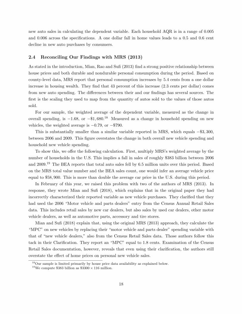
2.4 Reconciling Our Findings with MRS (2013)
As stated in the introduction, Mian, Rao and Sufi (2013) find a strong positive relationship between
house prices and both durable and nondurable personal consumption during the period. Based on
county-level data, MRS report that personal consumption increases by 5.4 cents from a one dollar
increase in housing wealth. They find that 43 percent of this increase (2.3 cents per dollar) comes
from new auto spending. The differences between their and our findings has several sources. The
first is the scaling they used to map from the quantity of autos sold to the values of those autos
sold.
For our sample, the weighted average of the dependent variable, measured as the change in
overall spending, is −1.68, or −$1, 680.18 Measured as a change in household spending on new
vehicles, the weighted average is −0.79, or −$790.
This is substantially smaller than a similar variable reported in MRS, which equals −$3, 300,
between 2006 and 2009. This figure overstates the change in both overall new vehicle spending and
household new vehicle spending.
To show this, we offer the following calculation. First, multiply MRS’s weighted average by the
number of households in the U.S. This implies a fall in sales of roughly $383 billion between 2006
and 2009.19 The BEA reports that total auto sales fell by 6.5 million units over this period. Based
on the MRS total value number and the BEA sales count, one would infer an average vehicle price
equal to $58, 900. This is more than double the average car price in the U.S. during this period.
In February of this year, we raised this problem with two of the authors of MRS (2013). In
response, they wrote Mian and Sufi (2018), which explains that in the original paper they had
incorrectly characterized their reported variable as new vehicle purchases. They clarified that they
had used the 2006 “Motor vehicle and parts dealers” entry from the Census Annual Retail Sales
data. This includes retail sales by new car dealers, but also sales by used car dealers, other motor
vehicle dealers, as well as automotive parts, accessory and tire stores.
Mian and Sufi (2018) explain that, using the original MRS (2013) approach, they calculate the
“MPC” on new vehicles by replacing their “motor vehicle and parts dealer” spending variable with
that of “new vehicle dealers,” also from the Census Retail Sales data. Those authors follow this
tack in their Clarification. They report an “MPC” equal to 1.8 cents. Examination of the Census
Retail Sales documentation, however, reveals that even using their clarification, the authors still
overstate the effect of home prices on personal new vehicle sales.
18Our sample is limited primarily by house price data availability as explained below.19We compute $383 billion as $3300 × 116 million.
18

Retail sales by new vehicle dealers include revenue from retailing new vehicles “in combination
with activities, such as repair services, retailing used cars and selling replacement parts and ac-
cessories.” Unless one could strip out the value of these other activities, one would overstate the
value of new cars sold in a particular county using the MRS approach. If, for example, a new car
dealership sold a new car for $30, 000 and took a trade in that it was able to resell for $25, 000,
then dealership would record $55, 000 in sales to the Census.20
Table 6 provides the definition of motor vehicle spending used in several papers as well as the
dollar amounts for those spending variables in 2006 and 2007. Mian, Rao and Sufi (2013) uses
amounts from Census Annual Retail Sales, which equals $900 billion in 2006. This is more than
double our measure used to compute the overall AQR and quadruple our measure used to compute
the household AQR, which are based on government-reported average auto prices. Replacing the
Mian, Rao and Sufi (2013) definition with “New Car Dealers” from Census Retail Sales includes
used car sales and dealership sales replacement parts and accessories.
Our measure for calculating the household AQR combines data on county-level new vehicle sales
quantities, the BTS average vehicle price and the share of new vehicles sold to consumers. In 2007,
this calculation implies new vehicle sales to consumers equal to $221 billion. We can check this
against Bureau of Economic Analysis aggregate data. Reassuringly, total personal consumption
expenditure on new motor vehicles reported by the BEA is very close to our number, equaling $233
billion in 2007.
An alternative approach would be to consider both new and used vehicles in constructing the
dependent variable. This would generate additional problems. First, the vehicle counts are based
on registration data. An auto handed down from a mother to a son in which the registration
changed would be counted as a sale. Similarly, someone moving a car’s registration from one state
to another would be counted as a sale, without having any offsetting reduction from the place where
the person relocated. More generally, there would remain an implicit double-or-more counting as
once-new cars were sold as used cars and those used cars were sold again as used cars. Also,
spending on used cars is not reflected in GDP. While potentially important for some questions,
the reshuffling of used vehicles amongst households does not directly impact the quantity of newly
produced goods and services in the economy.
There are two additional problems with using Census Retail Sales data. First, these data also
include some retail sales to businesses and government. If one is interested in the effect on household
purchases, then one must first strip out new vehicle sales to businesses and government.
Second, if one includes used car sales and motor vehicle parts stores, it is questionable whether
one should parse spending on these categories across counties based on their share of new car sales.
For instance, it is plausible that spending at motor parts stores would be higher rather than lower
in counties where fewer new cars were soldas individuals might spend relatively more on upkeep of
20The questionnaire sent by the Census to dealers states that, in filling out their surveys, the value of trade-insshould be included as partial payment.
19
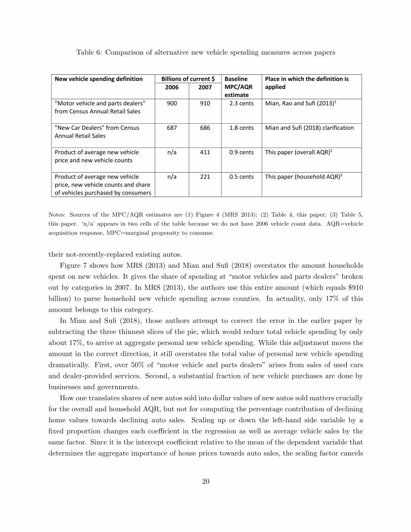
Table 6: Comparison of alternative new vehicle spending measures across papers
New vehicle spending definition Billions of current $ Baseline MPC/AQR estimate
Place in which the definition is applied 2006 2007
"Motor vehicle and parts dealers" from Census Annual Retail Sales
900 910 2.3 cents Mian, Rao and Sufi (2013)1
"New Car Dealers" from Census Annual Retail Sales
687 686 1.8 cents Mian and Sufi (2018) clarification
Product of average new vehicle price and new vehicle counts
n/a
411 0.9 cents This paper (overall AQR)2
Product of average new vehicle price, new vehicle counts and share of vehicles purchased by consumers
n/a 221 0.5 cents This paper (household AQR)3
Notes: Sources of the MPC/AQR estimates are (1) Figure 4 (MRS 2013); (2) Table 4, this paper; (3) Table 5,
this paper. ‘n/a’ appears in two cells of the table because we do not have 2006 vehicle count data. AQR=vehicle
acquisition response, MPC=marginal propensity to consume.
their not-recently-replaced existing autos.
Figure 7 shows how MRS (2013) and Mian and Sufi (2018) overstates the amount households
spent on new vehicles. It gives the share of spending at “motor vehicles and parts dealers” broken
out by categories in 2007. In MRS (2013), the authors use this entire amount (which equals $910
billion) to parse household new vehicle spending across counties. In actuality, only 17% of this
amount belongs to this category.
In Mian and Sufi (2018), those authors attempt to correct the error in the earlier paper by
subtracting the three thinnest slices of the pie, which would reduce total vehicle spending by only
about 17%, to arrive at aggregate personal new vehicle spending. While this adjustment moves the
amount in the correct direction, it still overstates the total value of personal new vehicle spending
dramatically. First, over 50% of “motor vehicle and parts dealers” arises from sales of used cars
and dealer-provided services. Second, a substantial fraction of new vehicle purchases are done by
businesses and governments.
How one translates shares of new autos sold into dollar values of new autos sold matters crucially
for the overall and household AQR, but not for computing the percentage contribution of declining
home values towards declining auto sales. Scaling up or down the left-hand side variable by a
fixed proportion changes each coefficient in the regression as well as average vehicle sales by the
same factor. Since it is the intercept coefficient relative to the mean of the dependent variable that
determines the aggregate importance of house prices towards auto sales, the scaling factor cancels
20

Table 7: Sales by motor vehicle and parts dealers in 2007, by category
New vehicles sold to consumers
17%
New vehicles sold to businesses and government
14%
New car dealers: Service and used car
sales52%
Other motor vehicle dealers5%
Automotive parts, access., and tire stores
6%Used car dealers
6%
Sources are Market IHS, Bureau of Economic Analysis, U.S. Census Bureau, Bureau of Transportation Statistics.
Total dollar value represented in the chart is spending at “motor vehicles and parts dealers,” which equaled $910
billion dollars in 2007.
21

out in the numerator and denominator. Thus the second main finding our paper—the inability of
house prices to explain much of the auto market collapse—is unrelated to the auto count scaling
issue.
One way to avoid having to set an auto price is to look at vehicle sales in logs. In this case,
the “units” drop out. If one regresses log changes in autos on log changes in house prices, the
resulting coefficient on house price changes will be an elasticity rather than an AQR (or MPC). In
an appendix to their paper, MRS run this elasticity regression.
As with the AQR regression, the intercept coefficient is of particular interest here. MRS report
in intercept equal to -0.366. This means that a county which experienced a zero house price shock
would be expected to see a 36.6 percent decline in auto sales between 2006 and 2009. Based on
aggregate data, new vehicle sales fell 47.1 percent over this period. Thus, 77 percent of the decline
in auto sales is unexplained by house price changes in the MRS regression. Once again, most of
the auto sales decline was unrelated to housing.
On another matter, one variable that we do not consider is a measure of total net worth. It
would be interesting to examine the influence of total net worth (housing and non-housing) on auto
sales. However, estimating net worth at the county-level requires financial wealth information,
which requires some imputation. MRS impute financial wealth by calculating the share of each
counties’ dividend plus interest earnings relative to national dividend plus earnings. They then
divide the aggregate financial wealth from the Flow of Funds according to those shares. Following
this procedure, we found that the weighted average of financial wealth equals over $300,000 per
household in 2007. By contrast, the median financial wealth from the Survey of Consumer Finances
in that year equaled $120, 000.21 As such, we interpret this imputation method as providing
unreliable results and do not study net worth.
Having a measure of net worth, which requires a measure financial wealth, would allow us to
estimate the effect of ”net worth shocks” as in MRS (2013) rather than home price or home value
shocks. The difference between net worth shocks and home price shocks is initial leverage. Kaplan,
Mitman and Violante (2016), however, show that after controlling for the change in home price
there is no statistically significant effect of initial leverage on nondurable consumption.
3 State-Level Panel Analysis
3.1 Data and Econometric Model
In this section, we compare the relationship between home prices and personal new vehicle sales
during the last recession period relative to the remainder of the last two decades. We cannot repeat
the exact analysis because of data limitations.
We lack vehicle count data before 2007, and instead use personal consumption expenditures
21Bucks et. al. (2009).
22

on motor vehicles in this section of the paper.22 This variable is available at the state level at an
annual rate beginning in 1997.23
Figure 4: Ratio of household debt to disposable personal income
.8
.9
1
1.1
1.2
Hou
seho
ld d
ebt t
o D
ispo
sabl
e in
com
e
1997q3 2002q3 2007q3 2012q3 2017q3
Quarter
Notes: Data sources are the Federal Reserve Board and the Bureau of Economic Analysis.
This will move us from a county-level quarterly analysis to a state-level annual one. Let Gi,t
denote the per capita motor vehicle consumption in state i in year t. The raw data are nominal
and we translate them into real series using the Consumer Price Index.
Our independent variable is based on county-level house price indices constructed by CoreLogic.
Our annual variable is averaged across monthly observations. State-level house price indices are
constructed by using the county-level averages weighted by the number of households in the county
22Motor vehicle consumption also includes motor vehicle parts.23Personal consumption expenditures of motor vehicles includes net purchases of used vehicles, measured as dealer
margins and net transactions, and the value of new vehicles purchased, as described in NIPA documentation. Dealermargins, for the most part, include the difference between the selling price and the dealer’s acquisition cost. Theyalso include wholesale margins for vehicles sold by wholesalers to dealers. According to NIPA documentation, nettransactions consist primarily of the “wholesale value of purchase by persons from dealers less sales by persons todealers.”
23
in 2007. We use home prices rather than home values on the right-hand side because the number
of homes is not available for the entire sample.
Our estimation equation is:
gci,t,δ = φδpci,t,δ + βδDi,t + vi,t,δ
for δ = 1, ...,H.
Census-region fixed effects, the lagged one-year growth rate of home prices and motor vehicle
consumption are included as controls. We estimate the model using least-squares at the 1-year,
3-year and 5-year horizons. To make estimates comparable, for each horizon we use the 5-year
horizon sample (which implies that we drop some observations for the shorter horizon regressions).
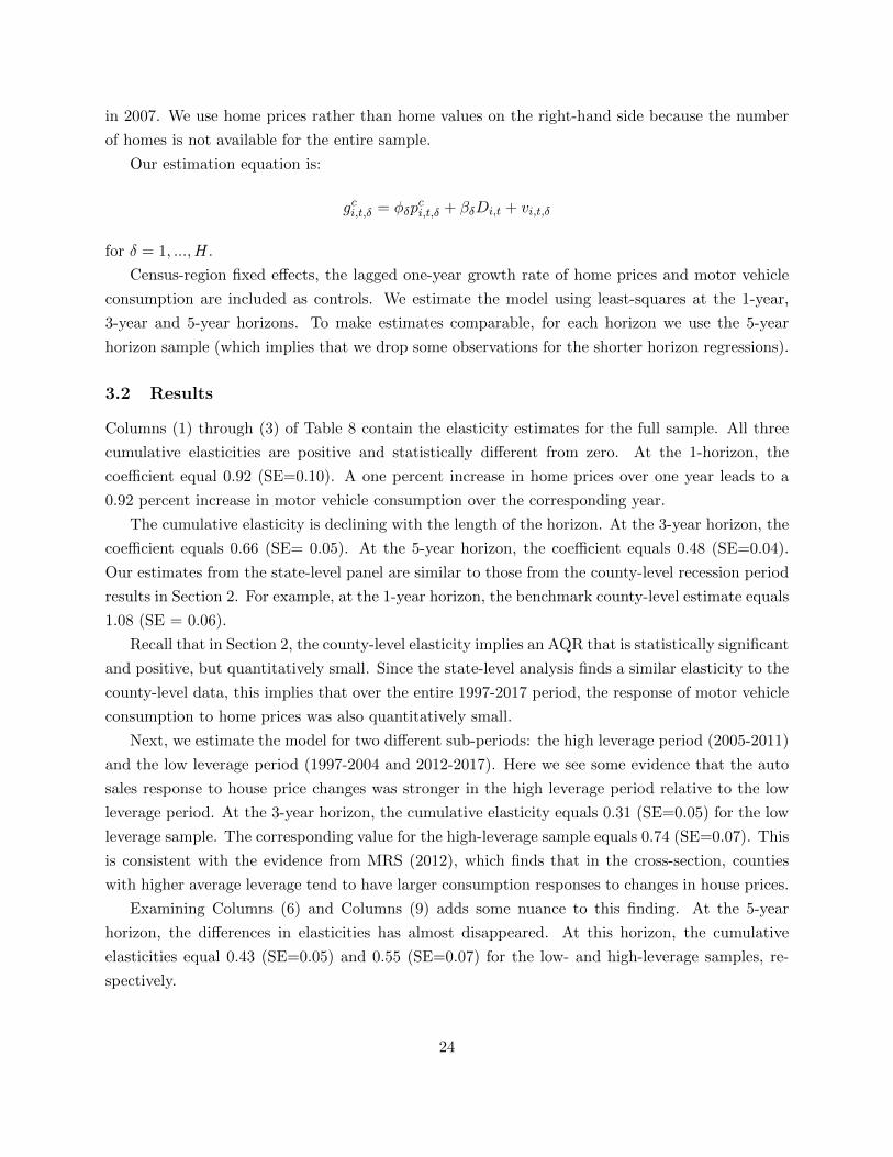
3.2 Results
Columns (1) through (3) of Table 8 contain the elasticity estimates for the full sample. All three
cumulative elasticities are positive and statistically different from zero. At the 1-horizon, the
coefficient equal 0.92 (SE=0.10). A one percent increase in home prices over one year leads to a
0.92 percent increase in motor vehicle consumption over the corresponding year.
The cumulative elasticity is declining with the length of the horizon. At the 3-year horizon, the
coefficient equals 0.66 (SE= 0.05). At the 5-year horizon, the coefficient equals 0.48 (SE=0.04).
Our estimates from the state-level panel are similar to those from the county-level recession period
results in Section 2. For example, at the 1-year horizon, the benchmark county-level estimate equals
1.08 (SE = 0.06).
Recall that in Section 2, the county-level elasticity implies an AQR that is statistically significant
and positive, but quantitatively small. Since the state-level analysis finds a similar elasticity to the
county-level data, this implies that over the entire 1997-2017 period, the response of motor vehicle
consumption to home prices was also quantitatively small.
Next, we estimate the model for two different sub-periods: the high leverage period (2005-2011)
and the low leverage period (1997-2004 and 2012-2017). Here we see some evidence that the auto
sales response to house price changes was stronger in the high leverage period relative to the low
leverage period. At the 3-year horizon, the cumulative elasticity equals 0.31 (SE=0.05) for the low
leverage sample. The corresponding value for the high-leverage sample equals 0.74 (SE=0.07). This
is consistent with the evidence from MRS (2012), which finds that in the cross-section, counties
with higher average leverage tend to have larger consumption responses to changes in house prices.
Examining Columns (6) and Columns (9) adds some nuance to this finding. At the 5-year
horizon, the differences in elasticities has almost disappeared. At this horizon, the cumulative
elasticities equal 0.43 (SE=0.05) and 0.55 (SE=0.07) for the low- and high-leverage samples, re-
spectively.
24

Tab
le8:
Cu
mu
lati
vere
spon
seel
asti
citi
esof
auto
sale
sto
hou
sep
rice
chan
ges
atva
riou
sh
oriz
ons
(sta
te-l
evel
pan
el,
leas
t-sq
uar
es)
Fu
llS
amp
leL
owL
ev.
Sam
ple
Hig
hL
ev.
Sam
ple
(1)
(2)
(3)
(4)
(5)
(6)
(7)
(8)
(9)
Coef
./S
EC
oef
./S
EC
oef
./S
EC
oef
./SE
Coef
./S
EC
oef
./S
EC
oef
./S
EC
oef
./S
EC
oef
./S
E
1-yr
HP
grow
th0.
918**
*-
-0.
417*
**-
-0.
932*
**-
-(0
.098)
(0.0
85)
(0.1
10)
3-yr
cum
HP
gro
wth
-0.
659*
**-
-0.
305*
**-
-0.
739*
**-
(0.0
52)
(0.0
50)
(0.0
73)
5-yr
cum
HP
gro
wth
--
0.48
0***
--
0.42
5***
--
0.54
8***
(0.0
39)
(0.0
52)
(0.0
69)
R2
0.4
20.
580.
620.
300.
500.
610.
350.
560.
63N
714
714
714
357
357
357
357
357
357
Note
s:T
he
dep
enden
tva
riable
isth
eacc
um
ula
ted
per
centa
ge
change
inauto
sale
sre
lati
ve
toa
yea
rt−
1base
line.
*p<
.1,
**p<
.05,
***p<
.01.
Reg
ress
ions
wei
ght
each
obse
rvati
on
by
the
num
ber
of
house
hold
sin
the
state
.E
ach
esti
mate
incl
udes
censu
s-re
gio
nfixed
effec
ts,
the
one
yea
rla
gof
the
one
yea
rgro
wth
rate
of
auto
sale
sand
house
pri
ces
as
contr
ols
.L
ev.
=le
ver
age.
25

Important dynamic considerations may influence how leverage interacts with housing wealth for
how individuals adjust auto sales. Highly leveraged individuals may choose or be forced to react
quickly in adjusting auto purchases when housing wealth falls, however, following the shock their
purchasing patterns begin to look more and more like the otherwise similarly affected low-leverage
households.
3.3 Miles Traveled and Home Prices
Because of its durability, investment in vehicles provides a poor basis to measure the marginal
utility of consumption of vehicle services. This marginal utility is better reflected by the service
flow from the stock of vehicles. We contend that vehicle miles travelled provides a more direct
measure of vehicle services provided. Therefore, we next estimate the relationship between the
growth in miles travelled and home prices.
Monthly miles traveled are available at the state-level from the Federal Highway Administration
beginning in 2006. We time-average monthly miles traveled up to the quarterly frequency. We
similarly take quarterly averages of the monthly house price data and aggregate these to the state
level using the weighted average the number of households in each county.
We then run regressions where the dependent variables are the analogous change in the log of
miles travelled at alternative horizons (1, 2 and 3-years). Our independent variable is the analogous
house price variables at the corresponding horizons.
We estimate the regression via least squares with weights given by the number of households
in each state and include state fixed effects in our baseline specification. These are presented in
Columns (1), (3) and (5) of Table 9. Columns (2), (4), and (6) add additional controls. These
are real income per household, the quarter-to-quarter growth rate in oil prices and the first lag
thereof. Including these additional variables has very little impact on house price elasticities at
every horizon.
Across each horizon and for alternative specifications, the elasticity is estimated within the
range 0.019 and 0.038. Each is statistically different from zero at conventional confidence levels.
Take for example Column (5), with an estimate of 0.038 (SE=0.016). If house prices on average
increase by 10 percent accumulated over a 3-year period, then one would expect a 0.38 percent
increase in vehicle miles travelled accumulated over the corresponding 3 years.
Thus, the effect of house prices on vehicle miles travelled is very small. By comparison, the
cumulative elasticity of vehicle sales to house price changes over a 3-year horizon, from Table 1,
equaled 0.60. The elasticity of house prices on vehicle sales, as we already explained was modest,
is more than fifteen times as large as the effect of home values on miles travelled.
There is little evidence that house price changes disrupted the service flow provided by vehicles
to a significant extent. Thus, households were able to smooth the effects of home price shocks on
their vehicle usage during the period. The economic model developed and calibrated in the next
26

Tab
le9:
Cu
mu
lati
vere
spon
seel
ast
icit
ies
ofm
iles
trav
eled
toh
ome
pri
cech
ange
sat
vari
ous
hor
izon
s(s
tate
-lev
elp
anel
,le
ast-
squ
ares
)
(1)
(2)
(3)
(4)
(5)
(6)
Coef
./S
EC
oef
./S
EC
oef
./S
EC
oef
./S
EC
oef
./S
EC
oef
./S
E
1-yr
cum
HP
gro
wth
0.03
5*0.
020
--
--
(0.0
21)
(0.0
21)
2-y
rcu
mH
Pgr
owth
--
0.03
6**
0.01
9-
-(0
.018
)(0
.017
)3-y
rcu
mH
Pgr
owth
--
--
0.03
8**
0.01
9(0
.016
)(0
.016
)L
agged
inco
me,
oil
pri
ces
No
Yes
No
Yes
No
Yes
R2
0.01
0.04
0.01
0.05
0.02
0.06
N21
9721
4721
9721
4721
9721
47
Note
s:T
he
dep
enden
tva
riable
isth
ecu
mula
tive
per
centa
ge
change
inm
iles
trav
eled
rela
tive
toa
yea
rt−
1base
line.
*p<
.1,
**p<
.05,
***p<
.01.
Reg
ress
ions
wei
ght
each
obse
rvati
on
by
the
num
ber
of
house
hold
sin
the
state
.E
ach
esti
mate
incl
udes
state
-fixed
effec
ts.
HP
=hom
epri
ce.
27
section is motivated by this observation: One can see a large change in investment in durable goods
alongside only a small change in the flow of services delivered by the stock of the durable good.
4 Expected Income and Auto Purchases
4.1 Survey Evidence on Economic Conditions
We look to individual-level survey data to find other potential explanations for the auto market col-
lapse besides house prices. The Michigan Survey of Consumers asks questions regarding consumers’
likelihood of buying a car as well as their reason for their answer.
Figure 5 plots the fraction of respondents who state that, in the current quarter, it is an
unfavorable time to purchase an auto over time. The figure shows an upward spike at the time of
the auto market collapse. The survey also asked respondents to state why it is either a favorable
or unfavorable time to purchase a car.
We take a subset of these responses and group them into one of two categories. The first
category is credit and debt conditions, both at the individual level and nationwide.24 The second is
economic conditions.25 Other categories, such as changes in the price of gasoline, are not included
here. Figure 6 plots the fraction of respondents who answered that it was an unfavorable time for
the reasons belonging to one of these groups.
The figure shows almost no change in the fraction motivated by credit and debt conditions and
a dramatic increase in the fraction motivated by economic conditions at the time of the collapse.
According to the MRS explanation, house prices declines during the period increased the net value
of household debt, inducing a negative wealth effect on auto purchases, and tighter borrowing
constraints. We take the nearly flat line for “credit/debt conditions” in Figure 6 as evidence
against the MRS explanation. On the other hand, the “economic conditions” reason motivates our
dynamic model of auto purchases, which uses shocks to current and expected future income as the
driving force for the auto market collapse.
Respondents are also asked about the expected future growth of their own homes’ values. This
allows us to compare the relative importance of house price expectations versus perceived economic
conditions on self-reported attitude towards auto buying. We estimate a probit regression of the
likelihood of buying a car dummy variable using a panel of respondents between 2004Q1 and
2018Q2. The left hand side variable equals 1 if the respondent answers that it is a favorable time
to buy a car in the current quarter. The right hand side variables are the expected percentage
increase in own home price, the probability of losing one’s own job over the next year, log income, a
dummy for whether the individual predicts favorable economic conditions over the next five years.
24The specific answers are described in survey documentation as: debt or credit is bad; larger/higher down paymentrequired; interest rates are high, will go up; and credit hard to get, tight money.
25The specific answers are: people cannot afford to buy now, times bad; people should save money, bad timesahead.
28

Figure 5: Fraction of individuals reporting that the current quarter is a bad time to buy an auto,1995Q1 to 2014Q4
1020
3040
50R
epor
ting
bad
time
to b
uy c
ar (%
)
1995q1 2000q1 2005q1 2010q1 2015q1Quarter
Notes: Source is Michigan Survey of Consumers.
29
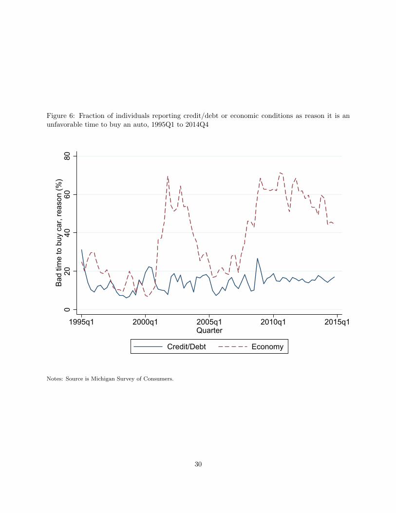
Figure 6: Fraction of individuals reporting credit/debt or economic conditions as reason it is anunfavorable time to buy an auto, 1995Q1 to 2014Q4
020
4060
80B
ad ti
me
to b
uy c
ar, r
easo
n (%
)
1995q1 2000q1 2005q1 2010q1 2015q1Quarter
Credit/Debt Economy
Notes: Source is Michigan Survey of Consumers.
30

Alternative specification include or exclude time and region fixed effects.26
Table 10: Marginal effect on probability of reporting that it is a good time to buy a car, 2004 -2018
(1) (2) (3) (4)Coef./SE Coef./SE Coef./SE Coef./SE
Percentage increase 0.005*** 0.005*** 0.006*** 0.004***in home price (0.000) (0.000) (0.000) (0.000)Positive 5-yr 0.173*** 0.173*** 0.176*** 0.171***economic outlook (0.005) (0.005) (0.005) (0.005)Prob of losing job -0.001*** -0.001*** -0.001*** -0.001***
(0.000) (0.000) (0.000) (0.000)Log of income 0.065*** 0.064*** 0.067*** 0.064***
(0.003) (0.003) (0.003) (0.003)Increase in home - - - 0.019***price (0.005)Decrease in home - - - -0.021***price (0.006)
Region FE Yes No Yes YesQtr FE Yes Yes No YesN 49466 49466 49466 49466
Notes: The dependent variable equals 1 if an agent views the present as a good time to buy a car. Data are from the
Michigan Survey of Consumers. * p < .1, ** p < .05, *** p < .01.
Table 10 displays the marginal effects in which explanatory variables are set equal to their
means in the sample. It shows that an individual’s personal view about the overall economy is
a key determinant of attitudes towards purchasing autos. Consider Column (1). Keeping other
variables at their means, an individual that moves their opinion about the economic performance
from positive to negative reduces the probability of having a positive car buying attitude by more
than 17 percent.
The regression also shows that although house price growth expectations influence car buying
attitudes, the marginal effect is small. According to column (1), an individual who expects their
house price to further decline by 1 percent from the average expectation sees an 0.5 percent reduc-
tion in having a positive attitude towards car buying. Columns (2) and (3) alter fix effects. The
results are nearly unchanged. Column (4) adds two dummy variables, whether own house price
increased over the past year and decreased over the next year. The coefficients are of the expected
sign, but have little impact on the remaining coefficients.
26Respondents are classified into one of four regions.
31

4.2 The Idea and the Mechanism
Next, we develop a permanent income model augmented with an auto-purchase choice to illustrate
the effect of expected income changes on the auto purchase decision. In the model, at multiple
points over their life, a household pays a fixed price to buy a new car. The utility associated
with owning a car is decreasing in the vehicle’s age. There are idiosyncratic shocks to income and
aggregate shocks to the growth rate of economy-wide average income. In the model, car owners
experience relatively small changes in the marginal disutility of holding on to an old vehicle when
expected income falls. Delaying auto replacement is an effective way to smooth the path of the
marginal utility of consumption in response to the negative shock.
The calibrated model exhibits a large short-run decline in new vehicle purchases in response
to weaker expected income growth going forward. A slowing of the real income growth rate to
-2 percent, similar to that experienced during the last recession, delivers an over 45 percent auto
sales decline on impact. This decline in auto sales is roughly equal to that experienced in the
second half of 2008. In contrast, a model that simply treated auto purchases as part of nondurable
consumption would have a elasticity that would be much too low to match the observed decline in
auto sales during the episode.
We abstract from several real-world features of the auto market, such as car loans and leasing.
The power of our approach is to show that, even absent these frictions, a largely standard permanent
income model can quantitatively replicate salient features of the 2008 auto market collapse.
We do not directly model the housing decision. This is because, earlier in the paper, we establish
that house price fluctuations explain only a small fraction of the auto sales decline. Moreover, for
many individuals, house prices are unlikely to influence the auto buying choice. For a homeowner
planning to stay put, a home price decline largely nets out to a zero effect because it reduces
tangible wealth but also increases the user cost of staying in the home. Also, survey data indicate
that very few individuals use home equity to purchase vehicles. For a renter not close to the margin
of buying a home, negative home price changes have no direct effect on own wealth and therefore
auto purchases. The effect on consumption for the two remaining groups, renters close to buying
homes and homeowners close to selling homes, work in opposite directions and therefore are likely
to be largely offset in the aggregate.
Finally, we note that our paper’s first two results—the quite limited role for house prices in
explaining the new auto sales decline—is established using cross sectional data without bringing
a specific economic model to the table. It might seem natural that we investigate the role of
income and future income expectations using cross sectional data as well. Unfortunately, highly
disaggregate (e.g., county-level) future income expectations data are not available. As such, we
change approaches by shifting to a calibrated economic model. Note, however, that we will use the
limited available survey data on future income expectations in calibrating our model.
32

4.3 The Model
Our model consists of a unit mass of households indexed i ∈ [0, 1]. Each household i earns an
exogenous stochastic income, and maximizes lifetime utility by choosing a stream of savings, non-
durable consumption, and vehicle purchases. We calibrate the model so that a period lasts one
year. The household buys only newly produced, i.e. not pre-owned cars.27
Let income be given by Yi,t = exp (yi,t)Zt, where Zt indexes aggregate income and evolves
according to Zt/Zt−1 = 1 + gt. Also, gt evolves according to a two-state Markov chain, {gL, gH},and yi,t evolves according to a first-order autoregression:
yi,t = ρyi,t−1 + εi,t (2)
where the innovation εi,t has mean zero, standard deviation σε and is i.i.d over time and household.
Let yi,−1 and Z−1 be positive and given as initial conditions.
The expected utility function is
Ui,t =∞∑j=0
βjEt
[UN
(Ci,t+j
)+ αUD (vi,t+j)
]
where Ci,t is consumption and vi,t is the vintage of the auto currently owned by the household, and
UN and UD give the period utility of nondurable and durable goods respectively. We assume the
utility is increasing and concave in nondurable consumption, and given as
UN
(C)
= log(C) (3)
We further assume that each household owns exactly one car, and the utility of owning a car
depends on the depreciated value of the car.
UD (v) = log(Pv,Car) (4)
With the depreciated value of a vintage v car given as
Pv,Car = (1− δv)P0,Car (5)
with δv giving the accumulated depreciation rate of a car that is v years old and P0,Car is the price
of a new car.
Next, the individual’s wealth Wi,t evolves according to:
Wi,t+1 = (1 + r) Wi,t + Yi,t − Ci,t − (P0,Car − Pv,Car)× 1 (vi,t+1 = 0)
27Our calibration will match data on autos originally purchased new. Thus, one should think about the new andpre-owned car markets as segmented, with our analysis solely focused on the former.
33

where borrowing is not allowed (i.e., Wi,t ≥ 0) and the price of buying a new auto is given as
(P0,Car − Pv,Car). This is the post trade-in cost of buying a new var.
To allow us to write the individual’s problem in recursive form we assume that the new car
price is a constant fraction of the current average income index: P0,Car = ZtP0,Car. Without
rising auto prices, as income trended upwards, the vehicle vintage distribution would pile up at
v = 0. Furthermore, this relationship between auto prices and income is reflected in the data. The
real price of autos generally increases over time; however, the price was flat during the 2007-2009
recession—the same time that income growth was very low. Note also that this assumption biases
us towards finding a smaller auto purchase response to the shock, because the price effect during
the low income growth period pushes individuals to purchase car prices (which rise in expected
price over time) sooner rather than later.
If we define Ci,t = Ci,t/Zt−1 and Wi,t = Wi,t/Zt−1, i.e. consumption and wealth, then we can
express the household i’s optimization problem recursively in the transformed system:
V (W, v, y, g) = max{VN (W, v, y, g) , VB (W, v, y, g)}
where VN and VB denote the values associated with car retention (i.e. not buying a new car) and
car replacement (i.e. buying a new car), respectively, with
VN (W, v, y, g) = maxC,W ′
{log (C) + α log(Pv,Car) + E
[S(W ′, v + 1, y′, g′
)|y, g
]}subject to:
W ′ +1
1 + gC =
1 + r
1 + gW + y
and
VB (W, v, y, g) = maxC,W ′
{log (C) + α log(Pv,Car) + E
[S(W ′, 0, y′, g′
)|y, g
]}subject to:
W ′ + (P0,Car − Pv,Car) +1
1 + gC =
1 + r
1 + gW + y
both with W ′i ≥ 0. The prime superscript advances time by one period.
Note that
v′ =
{0 if auto is purchased
v + 1 otherwise
To understand the household’s car buying decision let W = W (v; y, g) denote the level of W
that leaves a household with income level, y, and current car with vintage, v, indifferent between
car replacement and car retainment. The car replacement decision can then be written as
34
v′ =
{0 if W ≤ W
v + 1 if W ≥ W(6)
Given (6), we can explicitly define the evolution of the distribution of individuals over car
vintages. At each date, the fraction of individuals associated with each car vintage is given by
the predetermined vector Θt = {θv,y}, where each θv,y describes the number of individuals with
income level being y currently owning vintage v cars, and θ0,y denotes the number of individuals
with income y that replace their cars in the previous period. The evolution of the cross-sectional
distribution over time is determined as follows. Let αvy denote the vector of adjustment rates, then
the fraction of individuals associated with each car vintage in the support at Θ is summarized by
equations (7) and (8) below.
θ′0,y =∑∞
v=0 αv,yθv,y (7)
θ′v,y = θv−1,y(1− αv−1,y), v = 1, 2, ...,∞ (8)
4.4 Calibration
We start by assuming β = 0.94, which is a standard assumptions.
Next, we assume g ∈ (gL, gH) with transition matrix
Π =
[πL,L 1− πL,L
1− πH,H πH,H = 1
]
We use data from the Michigan Survey of Consumers to choose the values gL = −0.02 and gH =
0. Figure 7 plots the average one year ahead expected real growth of personal income across
respondents to the Michigan survey. Expected growth is for the upcoming year and subtracts each
respondents expected nominal income growth minus there expected inflation over the following
year. The figure shows a clear break around the time of the auto sales collapse. The red dashed
line is the average annual expected growth in 2006 and 2007. It equals approximately 0 percent.
The average annual expected growth over the following four years equals approximately -2 percent.
We assume that πL,L = 2/3, which is consistent with a decline in income growth that would
last 3 years in expectation, after which it would revert to its original growth path. Furthermore,
we set πH,H = 1 to indicate the economy is initially in steady state with a constant growth rate of
gSS = gH . This implies an expected decline in permanent income equal to 3.1 percent.28
To calibrate r, we rely on wealth data. In the standard permanent income model, if the economy
were in the high growth steady state, then given log preferences over nondurable consumption, the
28See the appendix for a derivation of this relationship.
35

Figure 7: Average one-year ahead real income growth expectations
-4-2
02
Exp
ecte
d re
al in
com
e gr
owth
(1-y
r for
war
d)
2006q3 2008q1 2009q3 2011q1 2012q3Quarter
Notes: Source is Michigan Survey of Consumers. For each quarter, we calculate the difference between
reported expected one-year ahead nominal income growth net of reported expected one-year ahead inflation.
36

real interest rate consistent with steady-state growth would be:
1 + r∗ = (1 + gSS) /β
In our model, this would lead to over savings with average wealth being too high. For this reason,
we introduce a wedge κ that lowers the rate of return on savings and thus discourages wealth
accumulation.
r =
(1 + gSS
β
)− 1− κ
We set κ = 0.005 Given the values of gSS and β, this implies r = 0.08 and implies a 3.1 percent
decline in expected permanent income by assuming πL,L = 0.66.
Next, we calibrate the vehicle cost P0,Car. The Kelly Blue Book price of a new vehicle in 2008
was approximately $27,000. Using a household income of $60,000, the average price of a car is 45%
of household income and thus we set P0,Car = 0.45.
To calibrate the accumulated depreciation rate of a car we look at the annual used car prices for
a 2006 Chervolet Malibu and a 2006 Honda Accord from when they were sold new in 2006 through
being 12 years old in 2018. We find that these cars roughly depreciated in value 30% during the
first year and then 15% on an accumulated basis every subsequent year. Thus, we set 1− δ1 = 0.7
and for v > 1 we set 1− δv = 0.7× 0.85v. 29 30
Finally, we set ρ = 0.95 and calibrate the standard deviation of the household’s income pro-
cess, σε, and the relative disutility, α, to match the empirical liquid assets/income ratio and the
distribution of car vintages, both for households that own a car that they bought new.
The empirical liquid assets/income ratio comes from the 2007 Survey of Consumer Finances
(SCF). Liquid assets are defined as the sum of money market accounts, checking accounts, saving
accounts, call accounts, and prepaid cards (variable: liq). Income includes wage income, business
farm income, rent incomes, interest & dividend income, self employed income, etc (variable: in-
come). In table 11 we compare various percentiles of the liquid asset/income ratio in both the SCF
data and the calibrated model. The SCF data is for the subsample of households that own at least
one car, van, minivan, SUV, or pickup that they bought new. Weights are accounted for when
calculating percentiles in the SCF data.
The car vintage distribution gives us the probability that a household x years later still owns
a car that they originally bought new. Figure 8 plots both the empirical distribution and the
distribution from our calibrated model. The empirical car vintage distribution comes for the 2007
Survey of Consumer Expenditures (CEX). To determine the distribution we consider all automo-
biles, trucks, minivans, vans, and SUVs. There is an unexplained dip in the distribution for new
29Many reasons have been proposed for this asymmetry in depreciation values. One explanation is the lemonsproblem which may be most severe for new cars as shown in House and Leahy (2004).
30We are now in the process of collecting used car price data on a wide variety of vehicles to ensure robustness ofthis calibration.
37

Table 11: Liquid Assets/Income Ratio
Percentile SCF Model
25th 0.04 0.0050th 0.11 0.1575th 0.30 0.4690th 0.75 1.0199th 3.80 3.13
Notes: Liquid Assets/Income Ratio = variable:liq/variable:income. The Survey Of Consumer Finance (SCF)data is from 2007 and for the subsample of households that own at least one car, van, minivan, SUV, orpickup that they bought new. Weights are accounted for when calculating percentiles in the SCF data.
Table 12: Parameter Values
Parameter Value Description Motivation
β 0.94 Discount factor Standard value for annual modelr 0.08 Interest rate Set a little below (1 + gSS)/β
P0,Car 0.45 Price of new car relative to income New car price = 45% of average income1− δ1 0.7 Car depreciation after 1 year Car depreciates 30% first year1− δv 0.7× 0.85v Car depreciation after v years and 15% every subsequent yearρ 0.95 Persistence of income level Standard value
gH = gSS 0.00 Steady state income growth rate From Michigan Survey of ConsumersgL −0.02 Steady state income growth rate From Michigan Survey of ConsumersπH,H 1.0 High to high transition probability High income growth is the steady stateπL,L 0.66 Low to low transition probability Set to match income slowdown expectationsσε 0.002 Standard deviation income shocks Set to match liquid asset/income distribution from SCFα 0.06 Relative utility consumption vs. car Set to match car vintage distribution from CEX
cars in year 0, possibly due to incomplete data.31 In calibrating our model we impute this value as
a linear trend based on data for one and two year old cars.
All the parameter values are summarized in Table 12.
4.5 The Solution Method and Policy Function
We solve the household’s problem by discrete discounted dynamic programming. We discretize the
wealth state space into H = 500 evenly spaced points between 0 and W = 80, the car vintage
distribution is capped at Jmax = 30, and the yi,t process is discretized on a grid with N = 8 points
using the Rouwenhorst method. The total state space has dimension 240,000 (= H × (2×N) ×(J + 1)). The value of W and Jmax are picked to ensure that the results are invariant to small
changes in them.
31We are working on figuring out the exact reason for this dip.
38

Figure 8: Distribution of auto vintages, data and economic model
0 5 10 15 20 25
Car Vintages/Age
0
0.05
0.1
0.15
% o
f Hou
seho
lds
Car Vintage Distribution (v)
ModelEmpirical (Actual)Empirical (Imputed)
Notes: The non-solid lines plots the 2007 distribution of vehicles, originally purchased new, and the solid
line plots the steady-state distribution from the economic model preceding the aggregate income growth rate
shock. The data comes from the Survey of Consumer Expenditures.
39

Figure 9: Policy function for auto replacement
Log wealth threshold for new car purchase
-1.5
-1.5
-1.5
-1.5
-1
-1
-1
-0.5
-0.5
-0.5
0
0
0
0.5
0.5
1
1
1
1.5
1.5
2
2
2
2.5
2.5
33
2 4 6 8 10 12 14
Vintage of current auto
-0.3
-0.2
-0.1
0
0.1
0.2
0.3
Log
of c
urre
nt in
com
e
Notes: The optimal policy at each point in the state space is described by a cutoff log wealth. Contour lines
reflect cutoffs with the value of log wealth labeling the corresponding contour line.
A household with wealth at or below W as defined in equation (6) will not replace his car.
Figure 9 plots this optimal cutoff wealth (in logs) as a function of the individual’s current income
(in logs) and vintage of their current auto. The cutoff wealths appears as numbers on the chart,
where those wealths label contour lines. For example, the contour labeled “2.5” gives pairs of
current incomes and vehicle vintages for which the cutoff log wealth equals 2.5. At these pairs, the
individual chooses to replace his auto if current log wealth is above 2.5 and does not replace if the
current log wealth is below 2.5.32 These policy functions assume the individual expects to remain
in the high average income growth state forever.
Each contour line is downward sloping, which implies that as current income falls, the individual
will replace older vehicles at the same cutoff level. Also, the cutoff wealth is falling as contour lines
move rightward and upward. This implies that the set of wealth values for which replacement is
optimal becomes larger as the individual has higher income or has an older vintage current auto.
32Vintages take on integer values, so the contour lines between integers on the x axis reflect interpolations.
40

5 Results from the Economic Model
We simulate the outcome of an household’s decision problem for a long history of T + Q periods.
For the first T periods, we assume Z grows at gSS = gH = 0. At period T + 1, average income
growth slows to gL = -2 percent and remains at -2 percent through T +Q. However, beginning at
T + 1 the forecasted law of motion for Zt evolves according to Π. That is, average income begins
each period in the low growth rate state and is expected to escape to the absorbing high growth
state with probability 1 − πH,H . In each period, the idiosyncratic determinant of income, εi,t, is
drawn according to the process described before.
Next, we set T = 1000, to ensure the initial conditions on a household’s state variables do not
affect are results, and Q = 5. We repeat this simulation for 100,000 households and present the
average results across these households. This ensures that the idiosyncratic paths of εi,t largely
cancel out in our final simulation.
Figure 10 plots the impulse responses for average income, auto sales and nondurable consump-
tion in response to an unanticipated slowdown in income growth that occurs at time zero. Each
variable is plotted as an index with base year t = −1. In the years preceding the shock, all three
variables grow at 0 percent annually. At period zero, average income growth unexpectedly be-
comes -2 percent and remains as such through period 5 (although households predict a 33 percent
chance each year that average income growth will increase to its initial steady-state growth rate of
0 percent.)
Nondurable consumption falls approximately 5 percent in response to the growth slowdown.
The decline in auto sales is much more dramatic. On impact, auto sales fall by over 40 percent.
This is consistent with the large decline seen during the 2008 auto-market collapse.
Our results show that a permanent income model augmented with an auto-purchase choice and
quantitatively calibrated can explain a large portion of the decline in car sales witnessed during
2008. As such the model also illustrates a mechanism to explain the auto market crash. Because
autos are a durable good, many individuals respond to the decline in expected permanent income
by delaying the replacement of their existing automobile. The impact on the marginal disutility of
having a slightly older car is smaller than the spike in marginal utility that would have occurred if
an individual had instead dramatically reduced their nondurable consumption.
Leahy and Zeira (2005) previously developed a theoretical exploration of our paper’s mechanism.
They study the cyclical behavior of both durable and non-durable consumption. Their simplifying
assumptions on preferences imply that consumers will not purchase small amounts of durable goods
early in their lifetime. Therefore, the shocks can be entirely absorbed by the changes in the purchase
timing of durable goods and non-durable consumption can be fully insulated from the aggregate
shocks.
Similar to Leahy and Zeira (2005), we study the role of the infrequent, discrete car replacement
decisions in explaining consumption behaviors over the business cycle, but assume a more general
41

Figure 10: Response of variables to income growth slowdown shock
-3 -2 -1 0 1 2 3 4 5Periods (shock arrives at period 0)
-50
-40
-30
-20
-10
0
10
20%
Dev
iatio
n fr
om S
tead
y S
tate
Response of variables to income-growth slowdown shock
Non-Durable ConsumptionAuto SalesIncome
Notes: Paths are aggregated across 100,000 individual paths from the initial steady-state wealth, income
and auto vintage distributions.
setting of preferences that implies households consume both durables and non-durable goods in
every period of their lifetime. Furthermore, we highlight how the standard permanent income
model augmented with a discrete car replacement decision can explain the large fall in auto sale in
the second half of 2008. We focus on the income shocks, which include both idiosyncratic shocks
to individual income and aggregate shocks to the growth rate of economy-wide average income.
The delay in the timing of auto replacement allows us to explain the large decline in auto purchase
in response to negative income shocks, which is essentially the mechanism of timing decisions as
emphasized in Leahy and Zeira (2005). Unlike their model, where non-durable consumption is fully
insulated from the aggregate shocks, the non-durable consumption in our model will falls following
the negative income shocks, which is consistent with the 2008 experience.
6 Conclusion
Nationwide, new auto sales collapsed in 2008. Using a calibrated, dynamic stochastic consumption-
savings model, we show that a widely experienced negative shock to permanent income is a strong
candidate explanation for the collapse. The explanation is consistent with the permanent income
hypothesis adapted to include infrequent, discrete durable goods purchases. House price declines,
on the other hand, explain only a small part of the auto sales decline.
42

A related explanation for the decline in auto sales is the increase in uncertainty that many
researchers have associated with the last recession.33 Bloom (2009) presents a model where ir-
reversible investment in durable goods causes an increase in uncertainty to reduce purchases of
durables. We note that a new vehicle purchase exhibits an aspect of irreversibility, because the
resale value of a newly bought new auto falls dramatically immediately after being acquired. Con-
sistent with this story, Hassler (2001) finds auto expenditures in the U.K. declined dramatically
with increases in uncertainty, proxied by stock market volatility.34
Our estimates speak to two important concepts in the economics of consumption: the permanent
income hypothesis (PIH) and consumption risk sharing. Our regressions do not directly test either
theory; however, our findings do not violate either theory in a quantitatively important way.
In its modern form, the PIH states that households attempt to smooth the marginal utility of
consumption in response to shocks. At a passing glance, it might seem that a 40 percent decline
in auto sales would be an obvious violation of the PIH. That view, however, would confound
investment in the durable good with the flow of services of the stock of durable goods. Based
on the generally smooth series for aggregate vehicle miles travelled before, during and after the
recession, one could conclude that the marginal utility from the services delivered by the stock of
autos was little affected by the shock that drove down house prices.
One implication of consumption risk sharing is that the marginal utility of consumption is
equated across regions even though shocks influence various regions with different intensities. The
decline in home prices was very heterogeneous across U.S. counties. A strong positive correlation be-
tween house price changes and auto sales changes would have indicated a breakdown of cross-region
consumption insurance. This strong positive correlation was not observed in the last recession, as
evidenced by our low estimated AQR. From a broader perspective, investment in durables pro-
vides a poor measure of the marginal utility of consumption of the durables as explained above.
Therefore, without additional structure on preferences or else different data, examining auto sales
regressions may constitute an inadequate approach for studying consumption risk sharing.
If, as we conjecture, households delayed replacing their existing autos with new ones in response
to economic shocks, then one could see utility-reducing changes on households apart from miles
traveled. For example, households may have spent additional dollars and time on maintaining used
cars that they would have otherwise replaced. The aggregate evidence for this channel is weak:
Based on the Census Annual Retail Sales data, spending at stores supplying automotive parts,
accessories and tires was nearly unchanged during the period.
Another possibility is that, although vehicle miles were smooth during the period, the typical
quality of the driving experience could have been diminished because households did not replace
their existing cars during the recession. For instance, those putting off buying a new car in cold
weather climates may not have been able to enjoy heated seats which were becoming more common
33See for example Baker, Bloom and Davis (2016) and Jurado, Ludvigson and Ng (2015).34See also Bertola, Guiso and Pistaferri (2005).
43

in new vehicles during this period.
Even though the service flow from auto usage (measured by miles traveled) was almost imper-
ceptibly disrupted during the last recession, the fall in auto demand did have dire consequences for
those working in the auto and related industries. The associated fall in labor demand from these
and other durable goods industries helped drive the national unemployment rate above 10 percent.
This, paired with imperfect labor income risk sharing, meant the bulk of the welfare costs from the
downturn was borne mainly by those who lost their jobs.
Understanding the strong sensitivity of demand for durable goods to economic shocks and how
this interacts with these sectors’ labor demand under imperfect labor income risk sharing merits
further research.
44
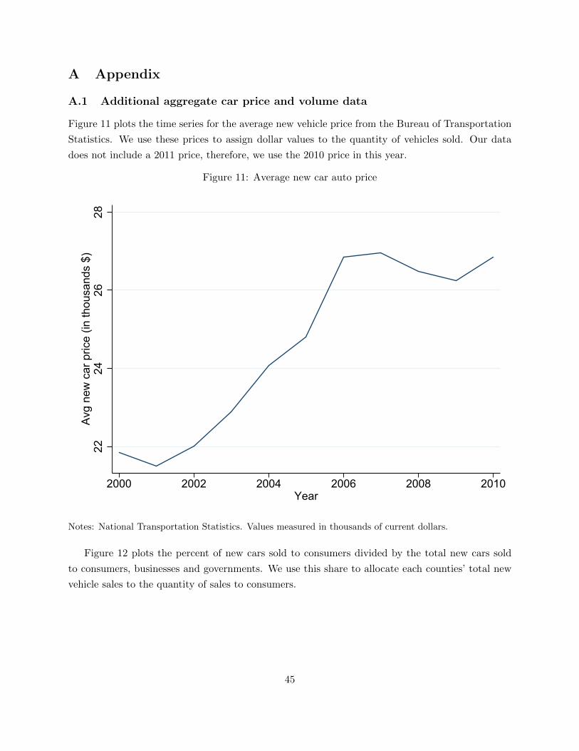
A Appendix
A.1 Additional aggregate car price and volume data
Figure 11 plots the time series for the average new vehicle price from the Bureau of Transportation
Statistics. We use these prices to assign dollar values to the quantity of vehicles sold. Our data
does not include a 2011 price, therefore, we use the 2010 price in this year.
Figure 11: Average new car auto price
2224
2628
Avg
new
car
pric
e (in
thou
sand
s $)
2000 2002 2004 2006 2008 2010Year
Notes: National Transportation Statistics. Values measured in thousands of current dollars.
Figure 12 plots the percent of new cars sold to consumers divided by the total new cars sold
to consumers, businesses and governments. We use this share to allocate each counties’ total new
vehicle sales to the quantity of sales to consumers.
45

Figure 12: Share retail sales of new cars to consumers
4550
5560
Per
cent
of n
ew c
ars
sold
to c
onsu
mer
s
2000 2005 2010 2015 2020Year
Notes: National Transportation Statistics, Table 1-18. The numerator is the quantity of cars sold to con-
sumers as a percentage of cars sold to consumers, businesses and governments.
46

A.2 Calibrating the average income process
The values of r, gH and gL are given in the body of the paper. Suppose that individuals hold that
income will remain in the low state for an expected length of 3 years. Given the Markov process
for income growth, this implies πL,L = 0.66.
To calibrate the expected present value of income in the low and high income process.
EPVL = 1 +πL,L (1 + gL)
1 + rEPVL +
(1− πL,L) (1 + gH)
1 + rEPVH
EPVH =1 + r
r − gH
Solving for the ratio of the two income processes:
EPVLEPVH
=r − gH
1 + r − πL,L (1 + gL)+
(1− πL,L) (1 + gH) (1 + r)
(r − gH) [1 + r − p (1 + gL)]
This implies that the expected decline in permanent income at the time of the shock equals 3.1
percent.
47

A.3 Additional Regression Specifications
This section contains additional regression results. The details of each specification are reflected in
the tables’ title and notes.
Table 13: Household new vehicle acquisition response (AQR) of sales to changes in home values,unweighted specification, county-level panel
(1) (2) (3)
Coef./SE Coef./SE Coef./SE
1-yr Cum Home Val 0.009*** - -
Change (0.001)
2-yr Cum Home Val - 0.007*** -
Change (0.000)
3-yr Cum Home Val - - 0.007***
Change (0.000)
Vehicles sold (lag -0.310** -0.645** -0.996**
change) (0.140) (0.287) (0.479)
House value (lag -0.003** -0.002 -0.007
change) (0.001) (0.003) (0.004)
Cash for Clunker FE 0.109*** 0.216*** 0.243**
(0.031) (0.066) (0.112)
Quarter 0.007*** 0.078*** 0.176***
(0.002) (0.005) (0.008)
R2 0.23 0.29 0.30
N 13673 13673 13673
Notes: The dependent variable is the cumulative change in vehicle sales to households at the appropriate horizon. *
p < .1, ** p < .05, *** p < .01. Regressions include seasonal fixed effects (not reported). Standard errors are robust
with respect to heteroskedacity and autocorrelation.
48

Table 14: Household new vehicle acquisition response (AQR) of sales to changes in home values,time fixed effects included, county-level panel
(1) (2) (3)
Coef./SE Coef./SE Coef./SE
1-yr Cum Home Val 0.004*** - -
Change (0.001)
2-yr Cum Home Val - 0.005*** -
Change (0.001)
3-yr Cum Home Val - - 0.006***
Change (0.001)
Vehicles sold (lag -0.195 -0.441 -0.673
change) (0.222) (0.462) (0.775)
House value (lag 0.002 0.009* 0.014*
change) (0.002) (0.005) (0.008)
R2 0.19 0.20 0.20
N 13673 13673 13673
Notes: The dependent variable is the cumulative change in vehicle sales to households at the appropriate horizon. *
p < .1, ** p < .05, *** p < .01. Regressions weight each observation by the number of households in the county and
include time fixed effects. Standard errors are robust with respect to heteroskedacity and autocorrelation.
49

Table 15: Household new vehicle acquisition responsee (AQR) of sales to changes in home values,Cash-for-Clunkers dummy in Fall 2009 only, county-level panel
(1) (2) (3)
Coef./SE Coef./SE Coef./SE
1-yr Cum Home Val 0.008*** - -
Change (0.001)
2-yr Cum Home Val - 0.006*** -
Change (0.001)
3-yr Cum Home Val - - 0.007***
Change (0.001)
Vehicles sold (lag - - -
change)
House value (lag 0.000 0.007 0.009
change) (0.003) (0.007) (0.011)
Cash for Clunker 0.287*** 0.477*** 0.639***
(Fall 09) FE (0.059) (0.125) (0.207)
Quarter 0.010*** 0.094*** 0.197***
(0.002) (0.005) (0.010)
R2 0.13 0.18 0.19
N 13673 13673 13673
Notes: The dependent variable is the cumulative change in vehicle sales to households at the appropriate horizon.
* p < .1, ** p < .05, *** p < .01. Regressions weight each observation by the number of households in the county
and includes seasonal fixed effects (not reported). Standard errors are robust with respect to heteroskedacity and
autocorrelation.
50

References
Adda, J. and R. Cooper (2000), “Balladurette and Juppette: A Discrete Analysis of Scrapping
Subsides,” Journal of Political Economy, 108, 4, 778-806.
Baker, S., N. Bloom and S. Davis (2016), “Measuring Economic Policy Uncertainty,” Quarterly
Journal of Economics, 131(4), 1593-1636.
Benmelech, E., R. Meisenzahl and R. Ramcharan (2017), “The Real Effects of Liquidity During the
Financial Crisis: Evidence from Automobiles,” Quarterly Journal of Economics, 132(1), 317-365.
Berger, D., V. Guerrieri, G. Lorenzoni and J. Varva (2018), “House Prices and Consumer Spending,”
Review of Economic Studies, Vol. 85, Issue 3, pp. 1502-1542.
Bernanke, B. (1984), “Permanent Income, Liquidity, and Expenditure on Automobiles: Evidence
From Panel Data,” Quarterly Journal of Economics, 99, 3, 587-614.
Bertola, G., L. Guiso and L. Pistaferri (2005), “Uncertainty and Consumer Durables Adjustment,”
The Review of Economic Studies, 72(4), 973-1007.
Bloom, N. (2009), “The Impact of Uncertainty Shocks,” Econometrica, 77(3), 623-685.
Bucks, B., A. Kennickell, T. Mach and K. Moore (2009), “Changes in U.S. Family Finances from
2004 to 2007: Evidence from the Survey of Consumer Finances,” Federal Reserve Bulletin, 95,
A1-A56.
Corbae, D. and E. Quintin (2015), “Leverage and the Foreclosure Crisis,” Journal of Political
Economy, Vol. 123, No. 1, pp. 1-65.
De Nardi, M., E. French and D. Benson (2012), “Consumption and the Great Recession,” Economic
Perspectives, Federal Reserve Bank of Chicago, QI, 1-16.
Disney, R., J. Gathergood and A. Henley (2010), “House Price Shocks, Negative Equity, and House-
hold Consumption in the United Kingdom,” Journal of the European Economic Association, 8(6),
1179-1297.
Dupor, B. and R. Guerrero (2017), “Local and Aggregate Fiscal Policy Multipliers,” Journal of
Monetary Economics, 92, 16-30.
Dupor, B. and R. Guerrero (2018), “The Aggregate and Relative Economic Effects of Medicaid
and Medicare Expansions,” Working Paper.
Eberly, J. (1994), “Adjustment of Consumers’ Durable Stocks: Evidence from Automobile Pur-
chases,” Journal of Political Economy, 102, 3, 403-436.
51

Favilukus, J., S. Ludvigson and S. Van Nieuwerburg (2016), “The Macroeconomic Effects of Housing
Wealth, Housing Finance and Limited Risk Sharing in General Equilibrium,” Journal of Political
Economy, Vol. 125, No. 1, pp. 140-223.
Garriga, C. and A. Hedlund (2017), “Mortgage Debt, Consumption, and Illiquid Housing Markets
in the Great Recession,” FRB St. Louis Working Paper No. 2017-30.
Glover, A., J. Heathcote, D. Krueger and J. Rıos-Rull (2017), “Intergenerational Redistribution in
the Great Recession,” Working Paper.
Hassler, J. (2001), “Uncertainty and the Timing of Automobile Purchases,” The Scandinavian
Journal of Economics, 103(2), 351-366.
House, C. and J. Leahy (2004), “An Ss Model with Adverse Selection,” Journal of Political Econ-
omy, 112, 581-614.
Jorda, O. (2005), “Estimation and Inference of Impulse Responses by Local Projections,” American
Economic Review, 95, 1, 161-182.
Jurado, K., S. Ludvigson and S. Ng (2015), “Measuring Uncertainty,” American Economic Review,
105(3), 1177-1216.
Kaplan, G., K. Mitman and G. Violante (2016), “Non-Durable Consumption and Housing Net
Worth in the Great Recession: Evidence from Easily Accessible Data,” NBER Working Paper
No. w22232.
Kaplan, G., K. Mitman and G. Violante (2017), “The Housing Boom and Bust: Model Meets
Evidence,” NBER Working Paper No. 23694.
Leahy, J. and J. Zeira (2005), “The Timing of Purchases and Aggregate Fluctuations,” Review of
Economic Studies, 72, 1127-1151.
Lehnert, A. (2004), “Housing, Consumption, and Credit Constraints,” FEDS Working Paper No.
2004-63.
McCully, B., K. Pence and D. Vine (2015), “How Much are Car Purchases Driven by Home Equity
Withdrawal? Evidence from Household Surveys,” FEDS Working Paper No. 2015-106.
Mian, A., A. Sufi (2018), “Household Balance Sheets, Consumption, and the Economic Slump: A
Clarification,” working paper.
Mian, A., K. Rao and A. Sufi (2013), “Household Balance Sheets, Consumption, and the Economic
Slump,” The Quarterly Journal of Economics, 128(4), 1687-1726.
52

Nakamura, E. and J. Steinsson (2014), “Fiscal Stimulus in a Monetary Union: Evidence from U.S.
Regions,” American Economic Review, 104(3), 753-92.
Poterba, J. (1991), “House Price Dynamics: The Role of Tax Policy and Demography,” Brookings
Papers on Economic Activity, 2, 143-203.
Ramey, V. and S. Zubairy (2017), “Government Spending Multipliers in Good Times and in Bad:
Evidence from U.S. Historical Data,” Journal of Political Economy, forthcoming.
Zimmerman, M. (1998), “A View of Recessions from the Automotive Industry, Beyond Shocks:
What Causes Business Cycles,” Federal Reserve Bank of Boston Conference Proceedings.
53