The 2k Factorial Design - site.iugaza.edu.pssite.iugaza.edu.ps/.../files/2010/02/CH6-The-2k-Factorial-Design1.pdf · Design of Engineering Experiments The 2k Factorial Design Special

The 2k Factorial Design

Dr. Mohammad Abuhaiba 1

HoweWork AssignmentDue Tuesday 1/6/2010

6.1, 6.2, 6.17, 6.18, 6.19


Design of Engineering ExperimentsThe 2k Factorial Design

Special case of the general factorial design; k factors, all at two levels

The two levels are usually called low and high (they could be either quantitative or qualitative)

It provides the smallest number of runs with which k factors can be studied in a complete factorial design.

Assumptions: Factors are fixed Completely randomized designs Usual normality assumptions are satisfied

Response is nearly linear over the range of the factors levels chosen


The 22 DesignChemical Process Example

Dr. Mohammad Abuhaiba

• Study the effect of concentration of reactant and amount of catalyst on conversion in a chemical process.

• “-” and “+” denote low and high levels of a factor

• Low and high are arbitrary terms

• Geometrically, the four runs form the corners of a square

• Factors can be quantitative or qualitative

4

Chemical Process Example


A = reactant concentration, B = catalyst amount,

y = recovery

5

Analysis Procedure for a Factorial Design

Estimate factor effects

Formulate model

Statistical testing (ANOVA)

Refine the model

Analyze residuals (graphical)

Interpret results


Estimation of Factor Effects


12

12

12

(1)[ (1)]

2 2

(1)[ (1)]

2 2

(1)[ (1) ]

2 2

nA A

nB B

n

ab a bA y y ab a b

n n

ab b aB y y ab b a

n n

ab a bAB ab a b

n n

7

Sum of Squares Sum of squares for any

contrast can be computed from Eq. 3-29

SST is given by Eq. 6-9

SST has 4n-1 DOF


2

2

2

(1)

(1)

(1)

(1)

4

(1)

4

(1)

4

A

B

AB

A

B

AB

Contrast ab a b

Contrast ab b a

Contrast ab a b

ab a bSS

n

ab b aSS

n

ab a bSS

n

8

Statistical Testing - ANOVA


Standards Order (Yates)Effests (1) a b ab

A -1 +1 -1 +1

B -1 -1 +1 +1

AB +1 -1 -1 +1


Treatment combination

Factorial effect

I A B AB

(1) + - - +

a + + - -

b + - + -

ab + + + +

10

The Regression Model

x1 is a coded variable that represents reactant concentration

x2 is a coded variable that represents amount of catlyst

Relationship between natural variables and cosed variables is given by:


1 1 2 2oy x x

1

2

/ 2

/ 2

/ 2

/ 2

high low

high low

high low

high low

con con con

con con

cat cat cat

cat cat

x x xx

x x

x x xx

x x

1

2

/ 2

/ 2

o grand average

A

B

11

The Response Surface


Residuals and Diagnostic Checking


The 23 Factorial Design


Effects in The 23 Factorial Design


See Eqs 6-11 to 6.17

for the factors' effects

A A

B B

C C

A y y

B y y

C y y

15


Table of – and + Signs for the 23

Factorial Design

16

Properties of the Table

Except for column I, every column has an equal number of + and –signs

The sum of the product of signs in any two columns is zero Multiplying any column by I leaves that column unchanged (identity

element) The product of any two columns yields a column in the table:

Orthogonal design Orthogonality is an important property shared by all factorial designs Each effect has a single DOF Sum of squares for any effect is:


2

A B AB

AB BC AB C AC

17

2

8

ContrastSS

n

Example of a 23 Factorial Design


Example 6-1: The Fill Height Experiment

RunCoded Factors Fill Height Deviation Factor Levels

A B C Replicate 1 Replicate 2 Low (-1) High (+1)

1 -1 -1 -1 -3 -1 A (%) 10 12

2 1 -1 -1 0 1 B (psi) 25 30

3 -1 1 -1 -1 0 C (bpm) 200 250

4 1 1 -1 2 3

5 -1 -1 1 -1 0

6 1 -1 1 2 1

7 -1 1 1 1 1

8 1 1 1 6 5


Estimation of Factor Effects

ANOVA

Model Coefficients – Full Model

Remove non-significant factors

Model Coefficients – Reduced Model

The AB interaction is significant at about 10%. Thus, there is some mild interaction between carbonation and pressure.

Run the process at low pressure and high line speed.

Reduce variablity in carbonation by controlling temperature more precisely

Example of a 23 Factorial Design

Model Summary Statistics for Reduced Model

R2 and adjusted R2

R2 for prediction (based on PRESS)


2

2 /1

/

Model

T

E EAdj

T T

SSR

SS

SS DOFR

SS DOF

2

Pred 1T

PRESSR

SS

20

Model Summary Statistics (pg. 222) Standard error of model coefficients (full model)

Confidence interval on model coefficients


2

ˆ ˆ( ) ( )2 2

E

k k

MSse V

n n

/ 2, / 2,ˆ ˆ ˆ ˆ( ) ( )

E Edf dft se t se

21

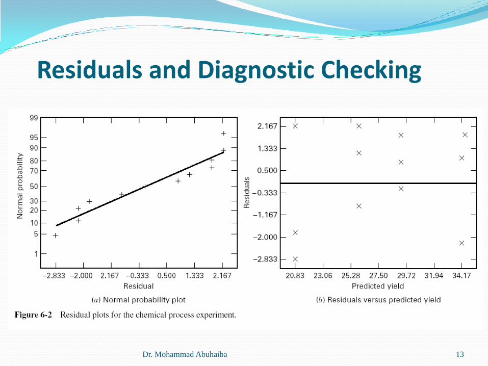
The General 2k Factorial Design There will be k main effects, and


two-factor interactions2

three-factor interactions3

1 factor interaction

k

k

k

22

The General 2k Factorial DesignAnalysis Procedure for a 2k Design

1. Estimate factor effects

2. Form initial model

3. ANOVA

4. Refine model

5. Analyze residuals

6. Interpret results


The General 2k Factorial DesignANOVA

The sign in each set of parentheses is negative if the factor is included in the effect and positive if the factor is not included.

Examples: 23 and 25 designs

Effects and sum of squares are estimated as


... ( 1)( 1)...( 1)AB KContrast a b k

...

2

... ...

2...

2

1

2

AB Kk

AB K AB Kk

AB K Contrastn

SS Contrastn


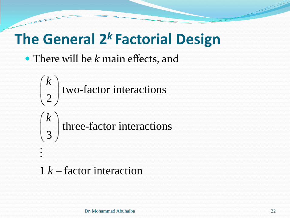
Unreplicated 2k Factorial Designs 2k factorial designs with one observation at

each treatment combination

An unreplicated 2k factorial design is also sometimes called a “single replicate”

Risks: If there is only one observation at each corner, is

there a chance of unusual response observations spoiling the results?

Modeling “noise”?


Unreplicated 2k Factorial Designs Spacing of Factor Levels in the

If the factors are spaced too closely, it increases the chances

that the noise will overwhelm the signal in the data

More aggressive spacing is usually best


Unreplicated 2k Factorial Designs Lack of replication causes potential problems

in statistical testing Replication admits an internal estimate of error

With no replication, fitting the full model results in zero degrees of freedom for error

Potential solutions to this problem Pooling high-order interactions to estimate error

Normal probability plotting of effects (Daniels, 1959)


Example of an Unreplicated 2k Design

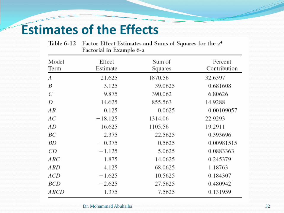
A 24 factorial was used to investigate the effects of four factors on the filtration rate of a resin

The factors are A = temperature, B = pressure, C = mole ratio, D= stirring rate

Experiment was performed in a pilot plant

Process engineer is interested in maximizing filteration rate.

Factor C currently at the high level

Would reduce formaldehyde concentration as much as possible.


The Resin Plant Experiment


The Resin Plant Experiment

Contrast Constants for the 2k DesignA B AB C AC BC ABC D AD BD ABD CD ACD BCD ABCD

{1} -1 -1 1 -1 1 1 -1 -1 1 1 -1 1 -1 -1 1a 1 -1 -1 -1 -1 1 1 -1 -1 1 1 1 1 -1 -1b -1 1 -1 -1 1 -1 1 -1 1 -1 1 1 -1 1 -1

ab 1 1 1 -1 -1 -1 -1 -1 -1 -1 -1 1 1 1 1c -1 -1 1 1 -1 -1 1 -1 1 1 -1 -1 1 1 -1

ac 1 -1 -1 1 1 -1 -1 -1 -1 1 1 -1 -1 1 1bc -1 1 -1 1 -1 1 -1 -1 1 -1 1 -1 1 -1 1

abc 1 1 1 1 1 1 1 -1 -1 -1 -1 -1 -1 -1 -1d -1 -1 1 -1 1 1 -1 1 -1 -1 1 -1 1 1 -1

ad 1 -1 -1 -1 -1 1 1 1 1 -1 -1 -1 -1 1 1bd -1 1 -1 -1 1 -1 1 1 -1 1 -1 -1 1 -1 1

abd 1 1 1 -1 -1 -1 -1 1 1 1 1 -1 -1 -1 -1cd -1 -1 1 1 -1 -1 1 1 -1 -1 1 1 -1 -1 1

acd 1 -1 -1 1 1 -1 -1 1 1 -1 -1 1 1 -1 -1bcd -1 1 -1 1 -1 1 -1 1 -1 1 -1 1 -1 1 -1

abcd 1 1 1 1 1 1 1 1 1 1 1 1 1 1 1



Estimates of the Effects


The Normal Probability Plot of Effects

The Half Normal Plot of Effects A plot of the absolute value of the effect estimates

against their cummulative normal probabilities.

Figure 6-15

The straight line always passes through the origin and should also pass close to the fiftieth percentile data value.



Main Effects and Interactions

Design Projection – Example 6-2 Because B is not significant and all interactions

involving B are negligible, we may discard B from the experiment so that the design becomes a 23 factorial in A, C, and D with two replicates.

ANOVA for the 23 design is shown in Table 6.13

By projecting the single replicate of the 24 into a replicated 23, we now have both an estimate of the ACD interaction and an estimate of error based on what is sometimes called hidden replication.


Design Projection – General Case If we have a single replicate of 2k design, and if h (h<k)

factors are negligible and can be dropped, then the original data correspond to a full two-level factorial in the remaining k – h factors with 2h replicates



ANOVA Summary for the Model


The Regression Model


Model Residuals


Model InterpretationResponse Surface Plots

With concentration at either the low or high level, high temperature and

high stirring rate results in high filtration rates


Example 6-3: The Drilling Experiment

A = drill load, B = flow, C = speed, D = type of mud,

y = advance rate of the drill


The Drilling Experiment Normal Probability Plot of Effects


Residual Plots

DESIGN-EXPERT Plot

adv._rate

Predicted

Re

sid

ua

ls

Residuals vs. Predicted

-1.96375

-0.82625

0.31125

1.44875

2.58625

1.69 4.70 7.70 10.71 13.71


The residual plots indicate that there are problems with the equality of varianceassumption

Employ a transformation on the response

Power family transformations are widely used

Transformations are typically performed to Stabilize variance

Induce normality

Simplify the model

Residual Plots

*y y


Selecting a Transformation

Empirical selection of lambda

Prior (theoretical) knowledge or experience can often suggest the form of a transformation


Effect Estimates Following Log Transformation

Three main effects are

large

No indication of large

interaction effects


ANOVA Following Log Transformation


Following Log Transformation


Addition of Center Points to a 2k

Design

Based on the idea of replicating some of the runs in a factorial design

Runs at the center provide an estimate of error and allow the experimenter to distinguish between two possible models:

0

1 1

2

0

1 1 1

First-order model (interaction)

Second-order model

k k k

i i ij i j

i i j i

k k k k

i i ij i j ii i

i i j i i

y x x x

y x x x x


no "curvature"F Cy y

The hypotheses are:

0

1

1

1

: 0

: 0

k

ii

i

k

ii

i

H

H

2

Pure Quad

( )F C F C

F C

n n y ySS

n n

This sum of squares has a

single degree of freedom


Example 6-6

4Cn

Usually between 3

and 6 center points

will work well

Design-Expert

provides the analysis,

including the F-test

for pure quadratic

curvature

Refer to the original experiment

shown in Table 6-10. Suppose that

four center points are added to this

experiment, and at the points x1=x2

=x3=x4=0 the four observed

filtration rates were 73, 75, 66, and

69. The average of these four center

points is 70.75, and the average of

the 16 factorial runs is 70.06.

Since are very similar, we suspect

that there is no strong curvature

present.


ANOVA for Example 6-6


If curvature is significant, augment the design with axial runs to create a central composite design. The CCD is a very effective design for fitting a second-order response surface model


Practical Use of Center Points (pg. 250) Use current operating conditions as the

center point

Check for “abnormal” conditions during the time the experiment was conducted

Check for time trends

Use center points as the first few runs when there is little or no information available about the magnitude of error

Center points and qualitative factors?


Center Points and Qualitative Factors

Documents

The 2k Factorial Design - site.iugaza.edu.pssite.iugaza.edu.ps/.../files/2010/02/CH6-The-2k-Factorial-Design1.pdf · Design of Engineering Experiments The 2k Factorial Design Special