Embed Size (px)
Citation preview
The Accident Externality from Driving2006
Aaron S. Edlin Pinar Karaca Mandic
From the Selected Works of Aaron Edlin;http://works.bepress.com/aaron edlin/21
931
[ Journal of Political Economy, 2006, vol. 114, no. 5]! 2006 by The University of Chicago. All rights reserved. 0022-3808/2006/11405-0004$10.00
The Accident Externality from Driving
Aaron S. EdlinUniversity of California, Berkeley and National Bureau of Economic Research
Pinar Karaca-MandicRAND Corporation
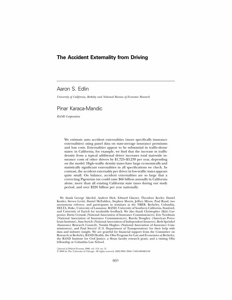
We estimate auto accident externalities (more specifically insuranceexternalities) using panel data on state-average insurance premiumsand loss costs. Externalities appear to be substantial in traffic-densestates: in California, for example, we find that the increase in trafficdensity from a typical additional driver increases total statewide in-surance costs of other drivers by $1,725–$3,239 per year, dependingon the model. High–traffic density states have large economically andstatistically significant externalities in all specifications we check. Incontrast, the accident externality per driver in low-traffic states appearsquite small. On balance, accident externalities are so large that acorrecting Pigouvian tax could raise $66 billion annually in Californiaalone, more than all existing California state taxes during our studyperiod, and over $220 billion per year nationally.
We thank George Akerlof, Andrew Dick, Edward Glaeser, Theodore Keeler, DanielKessler, Steven Levitt, Daniel McFadden, Stephen Morris, Jeffrey Miron, Paul Ruud, twoanonymous referees, and participants in seminars at the NBER, Berkeley, Columbia,DELTA, Duke, University of Lausanne, RAND, University of Southern California, Stanford,and University of Zurich for invaluable feedback. We also thank Christopher (Kitt) Car-penter, Davin Cermak (National Association of Insurance Commissioners), Eric Nordman(National Association of Insurance Commissioners), Rayola Dougher (American Petro-leum Institute), Sam Sorich (National Association of Independent Insurers), Beth Sprinkel(Insurance Research Council), Natalai Hughes (National Association of Insurance Com-missioners), and Paul Svercyl (U.S. Department of Transportation) for their help withdata and industry insight. We are grateful for financial support from the Committee onResearch at Berkeley, RAND Health, the Olin Program for Law and Economics at Berkeley,the RAND Institute for Civil Justice, a Sloan faculty research grant, and a visiting Olinfellowship at Columbia Law School.
932 journal of political economy
I. Introduction
Consider two vehicles that crash as one drives through a red light andthe other a green light. Assume that the accident would not occur ifeither driver took the subway instead of driving: hence, strictly speaking,both cause the accident in full, even though only one is negligent. Theaverage accident cost of the two people’s driving is the damages to twovehicles (2D) divided by the driving of two vehicles (i.e., D per drivenvehicle). But the marginal cost exceeds this. In fact, the marginal costof driving either vehicle is the damage to two vehicles (2D per drivenvehicle)—fully twice the average cost. Surprisingly, this observationholds just as much for the nonnegligent driver as for the negligent one.
Drivers pay the average cost of accidents (on average, anyway), notthe marginal cost, so this example suggests that there is a substantialaccident externality to driving, an externality that the tort system is notdesigned to address. The tort system is designed to allocate the damagesfrom an accident among the involved drivers according to a judgmentof their fault.
A damage allocation system can provide adequate incentives for care-ful driving, but it will not provide people with adequate incentives atthe margin of deciding how much to drive or whether to become adriver (Vickrey 1968; Green 1976; Shavell 1980; Cooter and Ulen 1988).Indeed, contributory negligence, comparative negligence, and no-faultsystems all suffer this inadequacy because they are all simply differentrules for dividing the cost of accidents among involved drivers and theirinsurers. Yet in many cases, from the vantage of causation, as distinctfrom negligence, economic fault will sum to more than 100 percent.Whenever it does, efficient driving incentives require that the driversin a given accident should in aggregate be made to bear more than thetotal cost of the accident, with the balance going to a third party suchas the government.
Does this theory of an accident externality from driving hold up inpractice? Equivalently, as a new driver takes to the road, does she in-crease the accident risk to others as well as assuming risk herself? If so,then a 1 percent increase in aggregate driving increases aggregate ac-cident costs by more than 1 percent. Such a positive connection betweentraffic density and accident risk will seem intuitive to anyone who findsherself concentrating more on a crowded highway and arriving hometired and stressed. Yet, such a relationship need not hold in principle.The riskiness of driving could decrease as aggregate driving increasesbecause increased driving could worsen congestion; and if people areforced to drive at lower speeds, accidents could become less severe orless frequent. Consequently, a 1 percent increase in driving could in-
accident externality from driving 933
crease aggregate accident costs by less than 1 percent and could evendecrease those costs.
The stakes are large. During our sample period, auto accident insur-ance in the United States cost over $100 billion each year, and totalaccident costs could have exceeded $350 billion each year after coststhat were not insured are included (National Association of InsuranceCommissioners, various years; Miller, Rossman, and Viner 1991). Multi-vehicle accidents, which are the source of potential accident external-ities, dominate these figures, accounting for over 70 percent of autoaccidents. If we assume that exactly two vehicles are necessary for multi-vehicle accidents to occur, then one might expect the marginal cost ofaccidents to exceed the average cost by 70 percent. Put differently, onewould expect aggregate accident costs to rise by 1.7 percent for every1 percent increase in aggregate driving, corresponding to an elasticityof accident costs with respect to driving of 1.7.1
Compared to its economic significance, there is relatively little em-pirical work gauging the size (and sign) of the accident externality fromdriving. Vickrey (1968), who was the first to conceptualize clearly theaccident externality from the quantity of driving (as opposed to thequality of driving), cites data on two groups of California highways andfinds that the group with higher traffic density has substantially higheraccident rates, suggesting an elasticity of the number of crashes withrespect to aggregate driving of 1.5.
A strand of transportation literature takes a similar cross-sectionalapproach and concentrates on the relationship between accident ratesand traffic volume (average daily traffic). Although this literature doesnot conceptualize the problem as one of an externality, that interpre-tation is appropriate: Belmont (1953) and Lundy (1965), for example,compared freeways with different average traffic volume and found thataccident rates increased with traffic volume; Belmont found that thetotal number of accidents per vehicle mile increased linearly with trafficuntil the traffic reached 650 vehicles per hour, after which it declined.More recently, Turner and Thomas (1986) examined various freewaysin Britain and reported similar findings. This literature matches upfreeways that the authors considered similar (e.g., four-lane highways)instead of doing panel analysis or using extensive controls.
Vickrey’s study and these cross-sectional transportation crash studies
1 Suppose that the chance that a driver causes an accident is p, that with probability .3pshe has a one-vehicle accident causing damage of D, and that with probability .7p she hasa two-vehicle accident causing damage of D to each vehicle. Since by assumption she isthe “but for” cause of each accident, the damages her driving causes are .3pD !
. This figure is also the marginal cost of driving per driver. The average2(.7pD) p 1.7pDcost of accidents per driver, however, is just pD. The elasticity of accident costs with respectto driving is the ratio of marginal to average cost.
934 journal of political economy
share limitations. Without knowledge of the inherent safety of the road-ways (roadway-specific effects), these studies could lead to biased esti-mates of how much traffic density increases accident rates on a givenroadway. If drivers are attracted to safer roads, then high-density roadscould end up with lower accident rates because the roads themselvesare inherently safer, not because traffic made them so. Likewise, if roadexpenditures are rational, then roads with more traffic will be betterplanned and better built in order to yield smoother traffic flow andfewer accidents. This again suggests that a cross-sectional study couldconsiderably understate the rise in accident risk with density on a givenroadway; in fact our regressions will suggest just these effects. Anotherdifficulty is that these crash studies contain no measure of accidentseverity: if congestion caused severity to decrease, then the accidentexternality would be smaller than these studies imply; in contrast, ifseverity increased with density (perhaps more vehicles per accident),then Vickrey (and implicitly these other studies) could dramaticallyunderstate the externalities. The “micro” nature of these studies is an-other limitation for most plausible policies on the state or federal level,where aggregate measures are required. One cannot, for example, knowthe appropriate level of a second-best corrective gasoline tax from suchstudies unless they are replicated across the full spectrum of roadwaytypes and they are combined with extensive micro-level data on drivingand traffic patterns (including a matrix of how drivers will shift drivingamong roadway risks as density changes).
This study is an attempt to provide better estimates of the size (andsign) of the aggregate accident externality from driving. To begin, wechoose a dependent variable, insurer costs, that is dollar-denominatedand captures both accident frequency and severity; we also analyze in-surance premiums as a dependent variable. We are concerned withaggregate effects across the full spectrum of driving in a given state.Our central question is whether one person’s driving increases otherpeople’s accident costs.
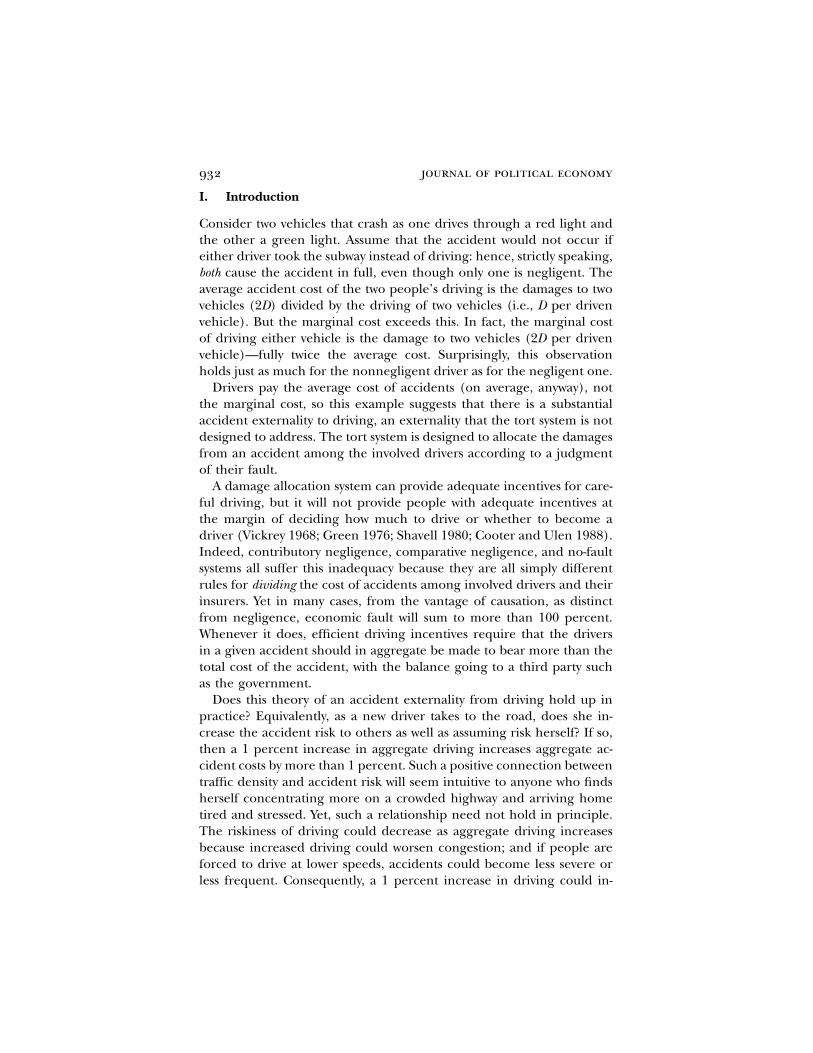
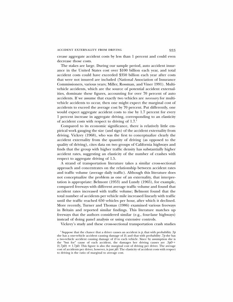
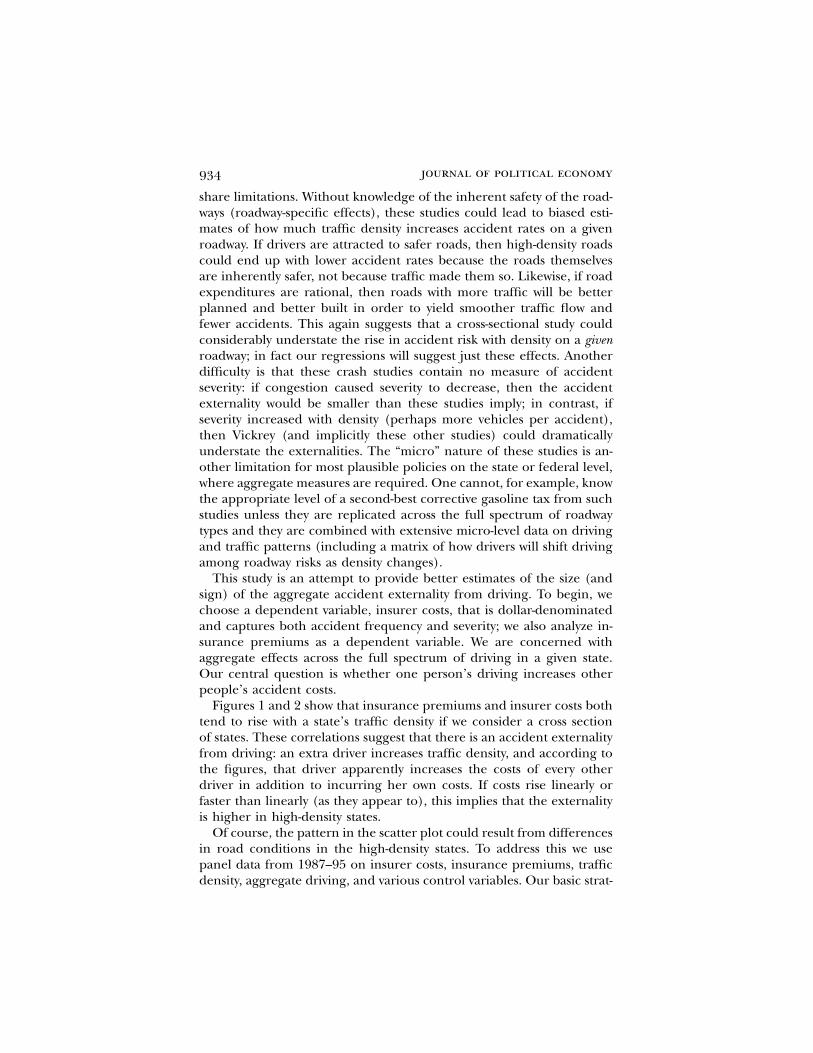
Figures 1 and 2 show that insurance premiums and insurer costs bothtend to rise with a state’s traffic density if we consider a cross sectionof states. These correlations suggest that there is an accident externalityfrom driving: an extra driver increases traffic density, and according tothe figures, that driver apparently increases the costs of every otherdriver in addition to incurring her own costs. If costs rise linearly orfaster than linearly (as they appear to), this implies that the externalityis higher in high-density states.
Of course, the pattern in the scatter plot could result from differencesin road conditions in the high-density states. To address this we usepanel data from 1987–95 on insurer costs, insurance premiums, trafficdensity, aggregate driving, and various control variables. Our basic strat-
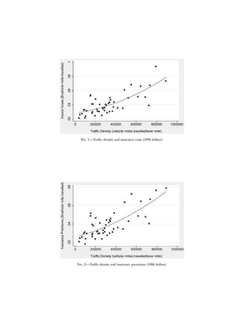
Fig. 1.—Traffic density and insurance costs (1996 dollars)
Fig. 2.—Traffic density and insurance premiums (1996 dollars)
936 journal of political economy
egy is to estimate the extent to which an increase in traffic density ina given state increases (or decreases) average insurer costs and insurancepremiums. Our regressions thereby provide a measure of the insuranceexternality of driving. Increases in traffic density can be caused by in-creases in the number of people who drive or by increases in the amountof driving each person does. To the extent that the external costs differat these two margins, our results provide a weighted average of thesetwo costs.
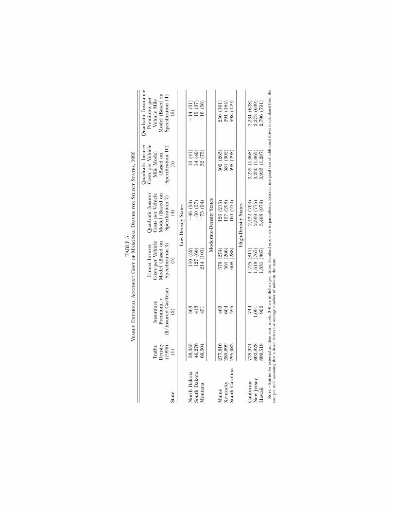
We find that traffic density increases accident costs substantiallywhether measured by insurer costs or insurance rates. This is robust toall our specifications; it is robust to linear and quadratic models, toinstrumental variables (IV) and ordinary least squares (OLS) estimation,and to cross-section or panel data. If congestion eventually reverses thiseffect, it occurs only at traffic densities beyond those in our sample.Indeed, our estimates suggest that a typical extra driver raises others’insurance rates (by increasing traffic density) by the most in high–trafficdensity states. In California, a very high-traffic state, we estimate that atypical additional driver increases the total statewide insurance costs by$1,725 " $817 to $3,239 " $1,068 each year, depending on the spec-ification. In contrast, in North Dakota, a very low-traffic state, we estimatethat others’ insurance costs are increased only slightly (and statisticallyinsignificantly): $10 " $41 each year, as shown in specification 10 oftable 5 below. These estimates of accident externalities pertain only toinsured accident costs and do not include the cost of injuries that areuncompensated or undercompensated by insurance, nor other accidentcosts such as traffic delays after accidents.
The remainder of this paper is organized as follows. Section II pro-vides a framework for determining the extent of accident externalities.Section III discusses our data. Section IV reports our estimation results.Section V presents a state-by-state analysis of accident externalities. Fi-nally, Section VI discusses the policy implications of our results anddirections for future research.
II. The Framework
Two vehicles can have an accident only if they are in proximity, and theprobability of proximity will increase with traffic density. In particular,let L equal the total number of lane miles, N be the number of drivers,and M equal the aggregate number of miles driven by all N drivers insome area. Consider the risk that a given driver i faces. With speed heldconstant and under the assumption that drivers make independent de-cisions about where to drive, the chance that another driver is in thesame location as i will be proportionate to the amount of driving thatthese other drivers do (i.e., ) and inversely propor-M[(N " 1)/N ] ! M

accident externality from driving 937
tional to the amount of roadway L over which this driving is distributed.Hence, for large N the probability of colocation will be proportionateto , which we will call the traffic density . Intuitively, theM/L D { M/Lmore other cars are on the road, the greater the chance that they willbe near me when I drive. If we assume that the probability or severityof accidents conditional on colocation does not depend on the traffic den-sity, then the expected rate r at which a representative driver-vehiclepair such as i bears accident costs would be affine in traffic density:
Mr p c ! c p c ! c D. (1)1 2 1 2L
The intercept, , represents the expected rate at which a driver incursc 1
a cost from one-vehicle accidents, and the second term, , representsc D2
the expected cost of two-vehicle accidents.2 Under the assumption thata vehicle’s annual driving is not a function of traffic density, one caninterpret r as the annual insurance cost associated with a representativevehicle. Some of our specifications do so. We will also estimate a modelthat abandons the assumption that driving quantity is independent oftraffic density. To do so, we will normalize accident costs by vehicle milesdriven instead of by the number of vehicles.
If we extend the model of equation (1) to consider accidents in whichthe proximity of three vehicles is required, we have
2r p c ! c D ! c D , (2)1 2 3
where the quadratic term accounts for the likelihood that two othervehicles are in the same location at the same time. Equations (1) and(2) are the two basic equations that we estimate.
The coefficients do not need to be interpreted as corresponding toone- and two-vehicle accidents. Equations (1) and (2) can alternativelybe viewed as a reduced-form model of accidents that accounts for thepossibility that risk depends on traffic density. In principle, the coeffi-cients c1, c2, and c3 need not be positive: as pointed out earlier, it ispossible that the probability/severity of a multivehicle accident couldbegin to fall at high traffic densities because traffic will slow down.
An average person pays the average accident cost r either by paying
2 Levitt and Porter (2001), in a similar model, estimate the relative crash risk of drunkdrivers using data on two-car crashes. Their model predicts that the number of accidentsinvolving two drunk drivers increases quadratically in the number of drunk drivers, whereasthe number involving a drunk driver and a sober driver has a linear relationship withboth the number of drunk drivers and the number of sober drivers. In fact, it is thisnonlinearity that allows them to identify the relative crash risk separately from relativerisk exposure. The Levitt-Porter nonlinearity corresponds with and with a negativec 1 02
accident externality. If one multiplies eq. (1) by the number of drivers, , where¯N p M/mis the miles driven per driver, one gets an equation for the total societal cost of accidentsm
that is quadratic in M or N much as in Levitt and Porter’s study.
938 journal of political economy
an insurance premium or by bearing accident risk. The accident ex-ternality from driving results (if is assumed to be positive) because ac 2
driver increases traffic density and thereby increases accident risks andcosts for other drivers. Although the increase in D from a single driverwill affect r only minutely, when multiplied by all the drivers who mustpay r, the effect could be substantial. The driver does not pay underany of the existing tort systems for exerting this externality.
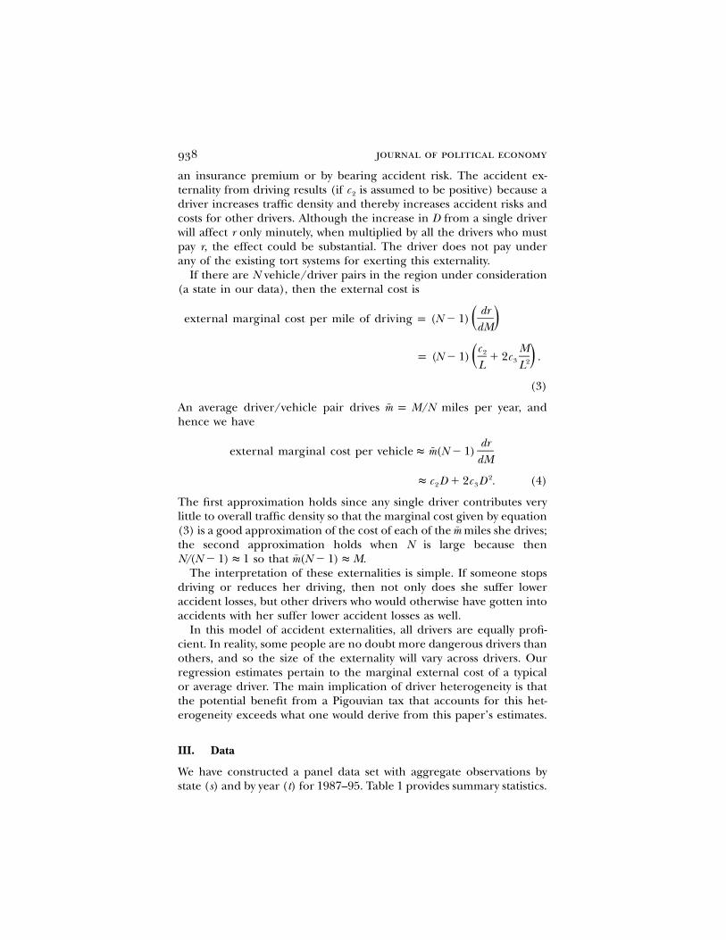
If there are N vehicle/driver pairs in the region under consideration(a state in our data), then the external cost is
drexternal marginal cost per mile of driving p (N " 1) ( )dM
c M2p (N " 1) ! 2c .3( )2L L
(3)
An average driver/vehicle pair drives miles per year, andm p M/Nhence we have
dr¯external marginal cost per vehicle ! m(N " 1)
dM2! c D ! 2c D . (4)2 3
The first approximation holds since any single driver contributes verylittle to overall traffic density so that the marginal cost given by equation(3) is a good approximation of the cost of each of the miles she drives;mthe second approximation holds when N is large because then
so that .¯N/(N " 1) ! 1 m(N " 1) ! MThe interpretation of these externalities is simple. If someone stops
driving or reduces her driving, then not only does she suffer loweraccident losses, but other drivers who would otherwise have gotten intoaccidents with her suffer lower accident losses as well.
In this model of accident externalities, all drivers are equally profi-cient. In reality, some people are no doubt more dangerous drivers thanothers, and so the size of the externality will vary across drivers. Ourregression estimates pertain to the marginal external cost of a typicalor average driver. The main implication of driver heterogeneity is thatthe potential benefit from a Pigouvian tax that accounts for this het-erogeneity exceeds what one would derive from this paper’s estimates.
III. Data
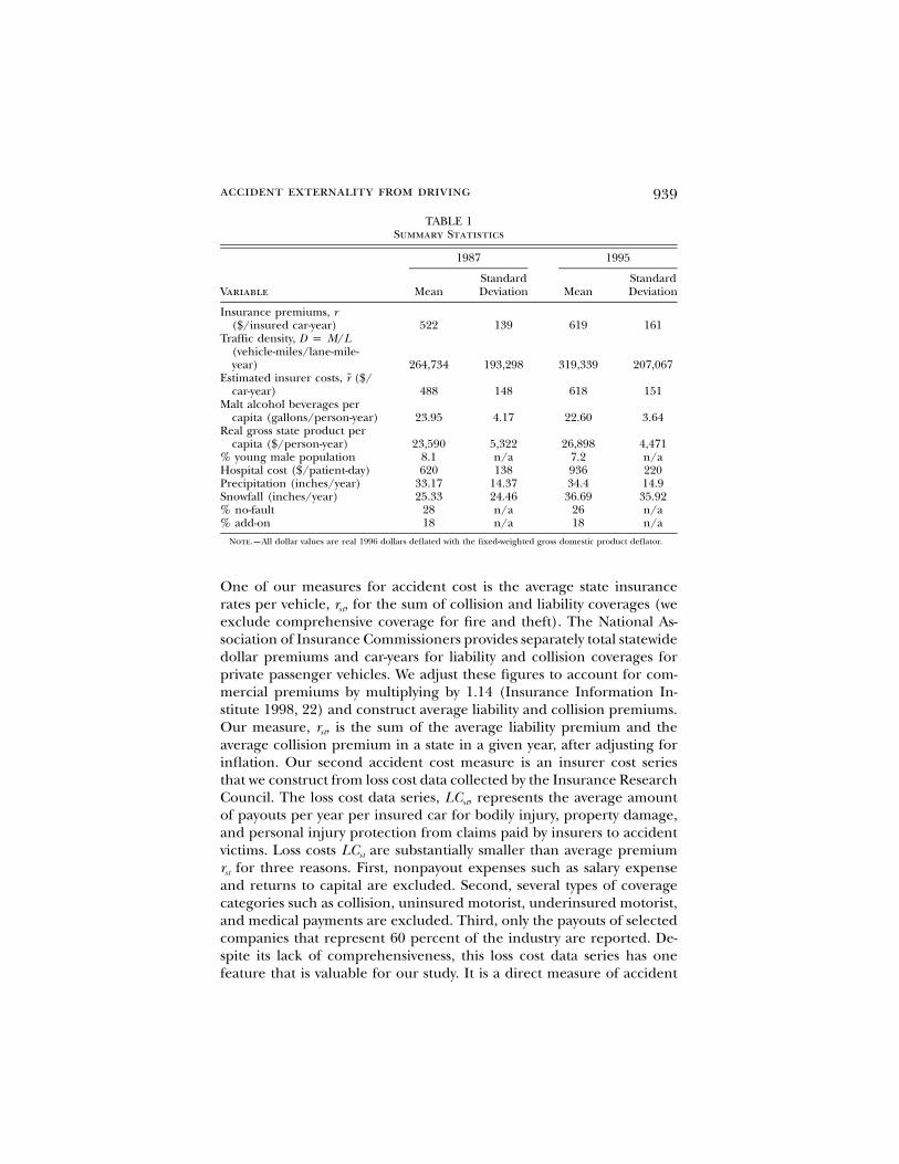
We have constructed a panel data set with aggregate observations bystate (s) and by year (t) for 1987–95. Table 1 provides summary statistics.
accident externality from driving 939
TABLE 1Summary Statistics
Variable
1987 1995
MeanStandardDeviation Mean
StandardDeviation
Insurance premiums, r($/insured car-year) 522 139 619 161
Traffic density, D p M/L(vehicle-miles/lane-mile-year) 264,734 193,298 319,339 207,067
Estimated insurer costs, ($/rcar-year) 488 148 618 151
Malt alcohol beverages percapita (gallons/person-year) 23.95 4.17 22.60 3.64
Real gross state product percapita ($/person-year) 23,590 5,322 26,898 4,471
% young male population 8.1 n/a 7.2 n/aHospital cost ($/patient-day) 620 138 936 220Precipitation (inches/year) 33.17 14.37 34.4 14.9Snowfall (inches/year) 25.33 24.46 36.69 35.92% no-fault 28 n/a 26 n/a% add-on 18 n/a 18 n/a
Note.—All dollar values are real 1996 dollars deflated with the fixed-weighted gross domestic product deflator.
One of our measures for accident cost is the average state insurancerates per vehicle, , for the sum of collision and liability coverages (werst
exclude comprehensive coverage for fire and theft). The National As-sociation of Insurance Commissioners provides separately total statewidedollar premiums and car-years for liability and collision coverages forprivate passenger vehicles. We adjust these figures to account for com-mercial premiums by multiplying by 1.14 (Insurance Information In-stitute 1998, 22) and construct average liability and collision premiums.Our measure, , is the sum of the average liability premium and therst
average collision premium in a state in a given year, after adjusting forinflation. Our second accident cost measure is an insurer cost seriesthat we construct from loss cost data collected by the Insurance ResearchCouncil. The loss cost data series, , represents the average amountLCst
of payouts per year per insured car for bodily injury, property damage,and personal injury protection from claims paid by insurers to accidentvictims. Loss costs are substantially smaller than average premiumLCst
for three reasons. First, nonpayout expenses such as salary expenserst
and returns to capital are excluded. Second, several types of coveragecategories such as collision, uninsured motorist, underinsured motorist,and medical payments are excluded. Third, only the payouts of selectedcompanies that represent 60 percent of the industry are reported. De-spite its lack of comprehensiveness, this loss cost data series has onefeature that is valuable for our study. It is a direct measure of accident
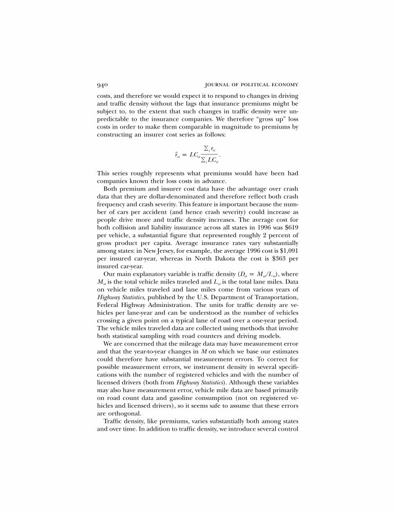
940 journal of political economy
costs, and therefore we would expect it to respond to changes in drivingand traffic density without the lags that insurance premiums might besubject to, to the extent that such changes in traffic density were un-predictable to the insurance companies. We therefore “gross up” losscosts in order to make them comparable in magnitude to premiums byconstructing an insurer cost series as follows:
! rsiir p LC .st st ! LCsii
This series roughly represents what premiums would have been hadcompanies known their loss costs in advance.
Both premium and insurer cost data have the advantage over crashdata that they are dollar-denominated and therefore reflect both crashfrequency and crash severity. This feature is important because the num-ber of cars per accident (and hence crash severity) could increase aspeople drive more and traffic density increases. The average cost forboth collision and liability insurance across all states in 1996 was $619per vehicle, a substantial figure that represented roughly 2 percent ofgross product per capita. Average insurance rates vary substantiallyamong states: in New Jersey, for example, the average 1996 cost is $1,091per insured car-year, whereas in North Dakota the cost is $363 perinsured car-year.
Our main explanatory variable is traffic density ( ), whereD p M /Lst st st
is the total vehicle miles traveled and is the total lane miles. DataM Lst st
on vehicle miles traveled and lane miles come from various years ofHighway Statistics, published by the U.S. Department of Transportation,Federal Highway Administration. The units for traffic density are ve-hicles per lane-year and can be understood as the number of vehiclescrossing a given point on a typical lane of road over a one-year period.The vehicle miles traveled data are collected using methods that involveboth statistical sampling with road counters and driving models.
We are concerned that the mileage data may have measurement errorand that the year-to-year changes in M on which we base our estimatescould therefore have substantial measurement errors. To correct forpossible measurement errors, we instrument density in several specifi-cations with the number of registered vehicles and with the number oflicensed drivers (both from Highway Statistics). Although these variablesmay also have measurement error, vehicle mile data are based primarilyon road count data and gasoline consumption (not on registered ve-hicles and licensed drivers), so it seems safe to assume that these errorsare orthogonal.
Traffic density, like premiums, varies substantially both among statesand over time. In addition to traffic density, we introduce several control
accident externality from driving 941
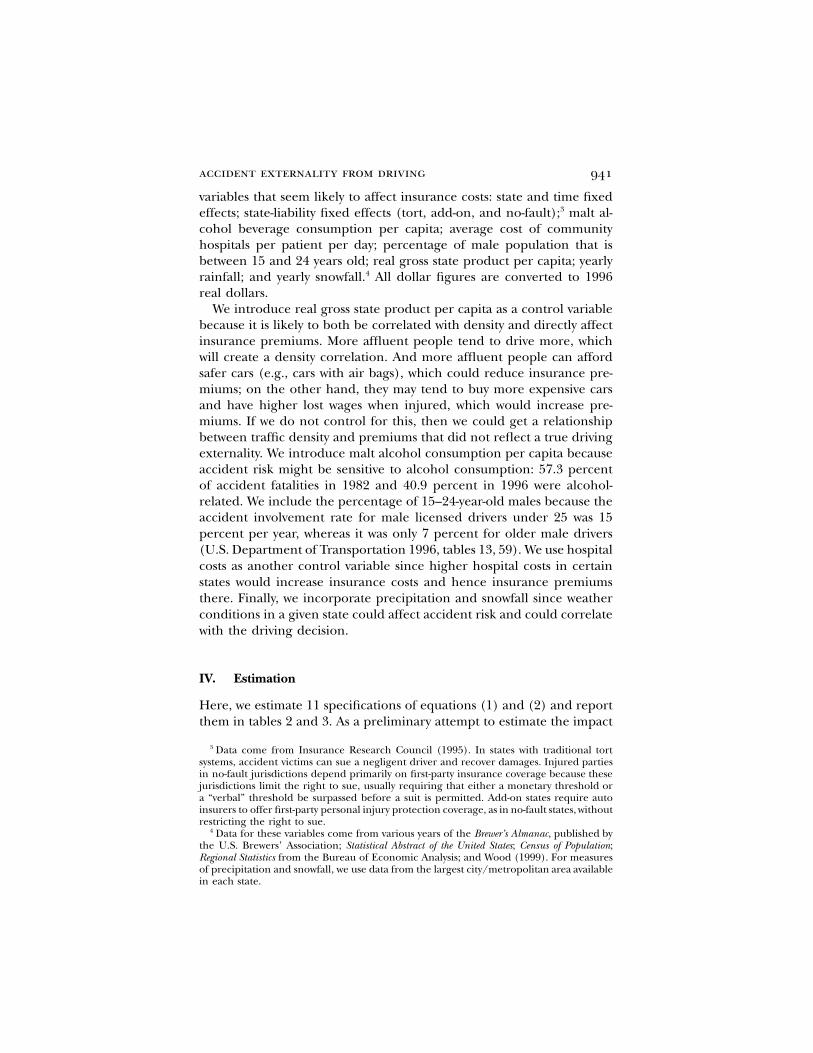
variables that seem likely to affect insurance costs: state and time fixedeffects; state-liability fixed effects (tort, add-on, and no-fault);3 malt al-cohol beverage consumption per capita; average cost of communityhospitals per patient per day; percentage of male population that isbetween 15 and 24 years old; real gross state product per capita; yearlyrainfall; and yearly snowfall.4 All dollar figures are converted to 1996real dollars.
We introduce real gross state product per capita as a control variablebecause it is likely to both be correlated with density and directly affectinsurance premiums. More affluent people tend to drive more, whichwill create a density correlation. And more affluent people can affordsafer cars (e.g., cars with air bags), which could reduce insurance pre-miums; on the other hand, they may tend to buy more expensive carsand have higher lost wages when injured, which would increase pre-miums. If we do not control for this, then we could get a relationshipbetween traffic density and premiums that did not reflect a true drivingexternality. We introduce malt alcohol consumption per capita becauseaccident risk might be sensitive to alcohol consumption: 57.3 percentof accident fatalities in 1982 and 40.9 percent in 1996 were alcohol-related. We include the percentage of 15–24-year-old males because theaccident involvement rate for male licensed drivers under 25 was 15percent per year, whereas it was only 7 percent for older male drivers(U.S. Department of Transportation 1996, tables 13, 59). We use hospitalcosts as another control variable since higher hospital costs in certainstates would increase insurance costs and hence insurance premiumsthere. Finally, we incorporate precipitation and snowfall since weatherconditions in a given state could affect accident risk and could correlatewith the driving decision.
IV. Estimation
Here, we estimate 11 specifications of equations (1) and (2) and reportthem in tables 2 and 3. As a preliminary attempt to estimate the impact
3 Data come from Insurance Research Council (1995). In states with traditional tortsystems, accident victims can sue a negligent driver and recover damages. Injured partiesin no-fault jurisdictions depend primarily on first-party insurance coverage because thesejurisdictions limit the right to sue, usually requiring that either a monetary threshold ora “verbal” threshold be surpassed before a suit is permitted. Add-on states require autoinsurers to offer first-party personal injury protection coverage, as in no-fault states, withoutrestricting the right to sue.
4 Data for these variables come from various years of the Brewer’s Almanac, published bythe U.S. Brewers’ Association; Statistical Abstract of the United States; Census of Population;Regional Statistics from the Bureau of Economic Analysis; and Wood (1999). For measuresof precipitation and snowfall, we use data from the largest city/metropolitan area availablein each state.
942 journal of political economy
TABLE 2Linear Insurance Rate Model, 1987–95
Regressor
Dependent Variable: InsurerCosts per Vehicle, r
Dependent Variable:Insurance Premiums
per Vehicle, r
OLS (1995Only)
(1)OLS(2)
IV(3)
OLS(4)
IV(5)
Traffic density, D .00042**(.00009)
.00058**(.00029)
.0019**(.0009)
.00036**(.00018)
.0014**(.00067)
State dummyvariables
No Yes Yes Yes Yes
Time dummyvariables
No Yes Yes Yes Yes
Malt alcohol bever-ages per capita
8.80*(4.54)
"2.04(5.63)
.43(5.87)
.79(2.44)
2.80(2.99)
Real gross productper capita
6,535.20*(3,779.90)
5,373.50(3,985.50)
2,224.50(4,866.50)
2,463.41(2,388.40)
"113.00(3,245.50)
Hospital cost .16**(.08)
".30**(.12)
".40**(.15)
.02(.05)
".05(.07)
% young malepopulation
30.99(27.83)
"4.98(14.52)
".75(14.92)
8.18(8.13)
11.64(9.45)
Precipitation 1.90**(.92)
.10(.36)
.06(.37)
".49*(.29)
".53*(.33)
Snowfall .32(.41)
.01(.22)
".07(.23)
".12(.12)
".19(.14)
No-fault 95.02**(32.08)
150.11**(17.04)
175.07**(28.06)
95.87**(8.80)
116.29**(18.40)
Add-on "1.35(37.59)
210.06**(51.66)
251.52**(58.46)
139.60**(39.48)
173.52**(43.74)
2R .73 .92 .91 .97 .96Durbin-Wu-Haus-
man test x2(1) p 13.42 x2(1) p 24.96H0: Traffic density is
exogenousp-value p .00 p-value p .00
Hansen’s J-statisticfor overidentify-ing restrictions
x2(1) p 1.17p-value p .28
x2(1) p .16p-valuep .69
Note.—Newey-West standard errors that account for heteroskedasticity and autocorrelation are reported in paren-theses below coefficients. IV uses as instruments registered vehicles per lane mile, licensed drivers per lane mile, timeand state dummy variables, and all the control variables. The number of observations for the panel is 450.
* Significant at the 10 percent level.** Significant at the 5 percent level.
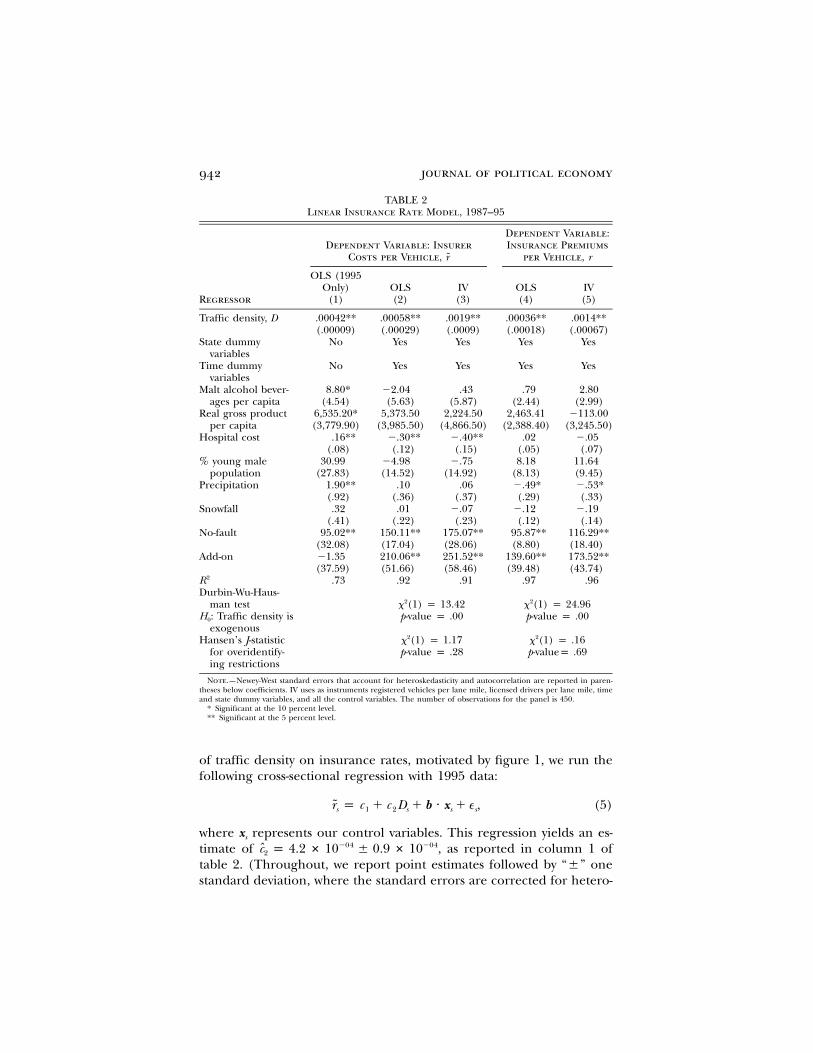
of traffic density on insurance rates, motivated by figure 1, we run thefollowing cross-sectional regression with 1995 data:
r p c ! c D ! b 7 x ! e , (5)s 1 2 s s s
where represents our control variables. This regression yields an es-xs
timate of , as reported in column 1 of"04 "04c p 4.2 # 10 " 0.9 # 102
table 2. (Throughout, we report point estimates followed by “"” onestandard deviation, where the standard errors are corrected for hetero-
accident externality from driving 943
skedasticity and autocorrelation using the method of Newey and West[1987].)
These cross-sectional results do not account for the potential corre-lation of state-specific factors (such as road conditions) with traffic den-sity. In particular, states with high accident costs would rationally spendmoney to make roads safer. Since this effect will work to offset the impactof traffic density, we would expect a cross-sectional regression to un-derstate the effect of density holding other factors constant. Moreover,downward biases result if states switch to liability systems that insure asmaller percentage of losses in reaction to high insurance costs.
To address this possibility we identify density effects from within-statechanges in density, using panel data to estimate the following model:
r p a ! g ! c ! c D ! b 7 x ! e . (6)st s t 1 2 st s st
This specification includes state fixed effects as and time fixed effectsgt, so that our identification of the estimated effect of increases in trafficdensity comes from comparing changes in traffic density to changes inaggregate insurer cost in a given state, controlling for overall timetrends. Including time fixed effects controls for technological changesuch as the introduction of air bags or other shocks that hit statesrelatively equally. As expected and as reported in column 2 of table 2,this specification yields larger estimates than the pure cross-sectionalregressions in specification 1. Specification 2 has a density coefficientof compared with"04 "04 "04 "045.8 # 10 " 2.9 # 10 4.2 # 10 " 0.9 # 10in specification 1.
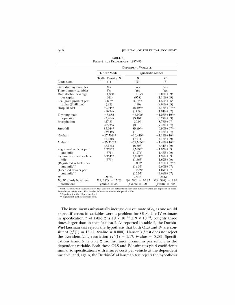
Measurement errors in the vehicle miles traveled variable M couldbias the traffic density coefficient toward zero in both specifications 1and 2. Therefore, we also perform IV estimation using licensed driversper lane mile and registered vehicles per lane mile as instruments fortraffic density. As justified above in Section III, we assume that anymeasurement error in these variables is uncorrelated with errors inmeasuring traffic density. These variables do not enter our accidentmodel directly because licensed drivers and vehicles by themselves getinto (almost) no accidents. A licensed driver can increase the accidentrate of others only to the extent that she drives, and vehicles, only tothe extent that they are driven; hence only through M. On the otherhand, these variables seem likely to be highly correlated with trafficdensity; in fact they are both positively correlated and jointly and in-dividually highly significant as seen in column 1 of table 4, which givesour first-stage regressions. Column 1 in table 4 reports the first-stageregression for our linear model represented in equation (1). We rejectthe null hypothesis that the instruments are jointly statistically insignif-icant with a p-value of 0.00.
944
TAB
LE3
Qua
drat
icIn
sura
nce
Rat
eM
odel
,198
7–95
Reg
ress
or
Dep
ende
ntVa
riab
le:I
n-su
rer
Cos
tspe
rVe
hic
le,r
Dep
ende
ntVa
riab
le:I
nsur
-an
cePr
emiu
ms
per
Veh
icle
,r
Dep
ende
ntVa
riab
le:
Insu
rer
Cos
tspe
rM
ile
Dri
ven
Dep
ende
ntVa
riab
le:
Insu
ranc
ePr
emiu
ms
per
Mil
eD
rive
n
OLS (6)
IV (7)
OLS (8)
IV (9)
IV (10)
IV (11)
Traf
ficde
nsity
,D"
.000
40(.
0006
)"
.000
98(.
0009
)"
.000
57(.
0004
)"
.001
1**
(.00
05)
"1.
09E"
07(7
.39E
"08
)"
3.81
E"08
(5.6
5E"
08)
D2
1.05
E"09
*(6
.49E
"10
)2.
51E"
09**
(7.3
8E"
10)
9.94
E"10
**(4
.24E
"10
)2.
19E"
09**
(6.1
3E"
10)
2.22
E"13
**(8
.39E
"14
)1.
79E"
13**
(6.1
8E"
14)
Stat
edu
mm
yva
riab
les
Yes
Yes
Yes
Yes
Yes
Yes
Tim
edu
mm
yva
riab
les
Yes
Yes
Yes
Yes
Yes
Yes
Mal
tal
coho
lbev
erag
epe
rca
pita
"1.
84(5
.88)
".0
6(6
.43)
.97
(2.6
0)2.
40(3
.30)
.000
16(.
0004
).0
0057
*(.
0003
)
945
Rea
lgro
sspr
oduc
tpe
rca
pita
5,90
7*(3
,504
)4,
713
(3,5
88)
2,96
8(2
,064
)2,
037
(2,1
01)
".1
9(.
31)
".4
3*(.
26)
Hos
pita
lcos
t"
.30*
(.12
)"
.35*
*(.
15)
.03
(.05
)"
.009
(.07
)"
1E"
05(.
0000
1)"
3E"
6(6
.78E
"6)
%yo
ung
mal
epo
pula
tion
10.6
2(1
7.42
)34
.84*
(19.
96)
22.9
3**
(9.2
5)42
.68*
*(1
2.7)
.002
5(.
0016
).0
026*
*(.
0012
)Pr
ecip
itatio
n.1
2(.
3).1
1(.
33)
".4
8*(.
28)
".4
8*(.
29)
"4E
"05
(3E"
05)
"5E
"05
*(3
E"05
)Sn
owfa
ll"
.02
(.22
)"
.11
(.23
)"
.15
(.12
)"
.23*
(.14
)"
7E"
06(2
E"05
)"
3E"
05**
(1E"
05)
No-
faul
t14
0.85
**(1
9.38
)14
3.35
**(2
2.37
)87
.11*
*(7
.30)
88.7
9**
(9.9
6).0
08**
(.00
2).0
07**
(.00
1)A
dd-o
n19
8.23
**(4
8.66
)20
7.29
**(5
5.32
)12
8.40
**(3
8.70
)13
5.22
**(3
8.70
).0
18**
(.00
4).0
11(.
003)
2R
.92
.92
.97
.97
.91
.95
Dur
bin-
Wu-
Hau
sman
test
23.5
944
.78
53.3
011
9.70
H0:
Traf
ficde
nsity
isex
ogen
ous
pp
.00
pp
.00
pp
.00
pp
.00
Han
sen’
sJ-s
tatis
ticfo
rov
erid
entif
ying
rest
rict
ions
2p
p.3
7.1
1p
p.9
5.1
0p
p.9
51.
10p
p.5
8N
ote.
—N
ewey
-Wes
tsta
ndar
der
rors
that
acco
untf
orhe
tero
sked
astic
ityan
dau
toco
rrel
atio
nar
ere
port
edin
pare
nthe
ses
belo
wco
effic
ient
s.IV
uses
asin
stru
men
tsre
gist
ered
vehi
cles
per
lane
mile
,lic
ense
ddr
iver
spe
rla
nem
ile,t
ime
and
stat
edu
mm
yva
riab
les,
and
allt
heco
ntro
lvar
iabl
es.T
henu
mbe
rof
obse
rvat
ions
for
the
pane
lis
450.
*Si
gnifi
cant
atth
e10
perc
ent
leve
l.**
Sign
ifica
ntat
the
5pe
rcen
tle
vel.
946 journal of political economy
TABLE 4First-Stage Regressions, 1987–95
Dependent Variable
Linear Model Quadratic Model
RegressorTraffic Density, D
(1)D
(2)2D
(3)
State dummy variables Yes Yes YesTime dummy variables Yes Yes YesMalt alcohol beverage
per capita"1,338(940)
"1,058(958)
"2.03E!09*(1.10E!09)
Real gross product percapita ($millions)
2.80**(.92)
3.07**(.96)
1.39E!06*(8.03E!05)
Hospital cost 50.94**(16.74)
48.49**(17.39)
4.13E!07**(1.91E!07)
% young malepopulation
"3,882(3,264)
"5,992*(3,464)
"1.23E!10**(3.77E!09)
Precipitation 57.81(85.35)
39.96(83.10)
8.73E!07(7.44E!07)
Snowfall 83.04**(39.42)
85.49**(40.19)
9.96E!07**(4.45E!07)
No-fault "17,701**(7,030)
"16,415**(7,011)
"1.13E!10**(4.13E!09)
Add-on "25,716**(8,275)
"24,505**(8,326)
"1.43E!10**(5.41E!09)
Registered vehicles perlane mile
1,778**(671)
2,509**(1,274)
"1.95E!09(1.46E!09)
Licensed drivers per lanemile
3,354**(679)
5,068**(1,563)
1.92E!09(1.67E!09)
(Registered vehicles perlane mile)2
"8.52(14.33)
4.79E!07**(2.00E!07)
(Licensed drivers perlane mile)2
"15.22(15.57)
1.07E!07(2.04E!07)
2R .9975 .9975 .9962H0: IV jointly have zero
coefficientF(2, 382) p 17.23
p-value p .00F(4, 380) p 10.87
p-value p .00F(4, 380) p 9.99
p-value p .00Note.—Newey-West standard errors that account for heteroskedasticity and autocorrelation are reported in paren-
theses below coefficients. The number of observations for the panel is 450.* Significant at the 10 percent level.** Significant at the 5 percent level.
The instruments substantially increase our estimate of , as one wouldc 2
expect if errors in variables were a problem for OLS. The IV estimatein specification 3 of table 2 is , roughly three"04 "0419 # 10 " 9 # 10times larger than in specification 2. As reported in table 2, the Durbin-Wu-Hausman test rejects the hypothesis that both OLS and IV are con-sistent ( , p-value p 0.000). Hansen’s J-test does not reject2x (1) p 13.42the overidentifying restriction ( , p-value p 0.28). Specifi-2x (1) p 1.17cations 4 and 5 in table 2 use insurance premiums per vehicle as thedependent variable. Both these OLS and IV estimates yield coefficientssimilar to specifications with insurer costs per vehicle as the dependentvariable; and, again, the Durbin-Wu-Hausman test rejects the hypothesis
accident externality from driving 947
that both OLS and IV are consistent, and Hansen’s J-test does not rejectthe overidentifying restriction. The consistency of results across thesetwo models provides added confidence in our findings.
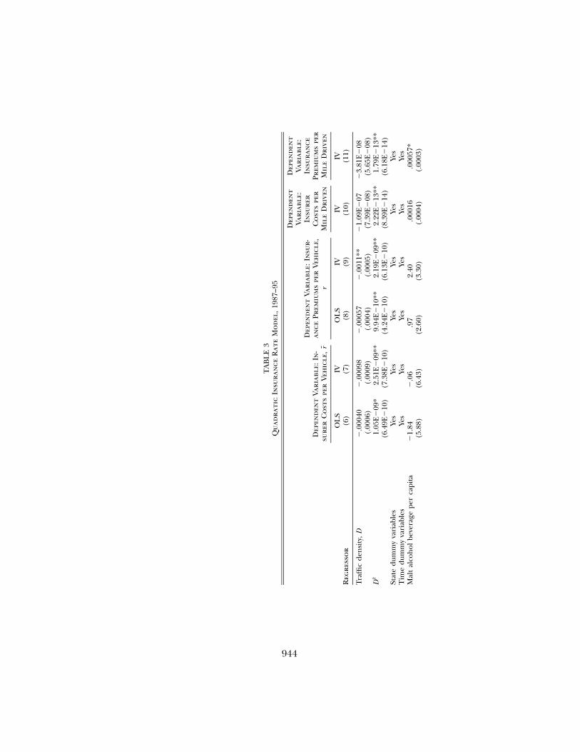
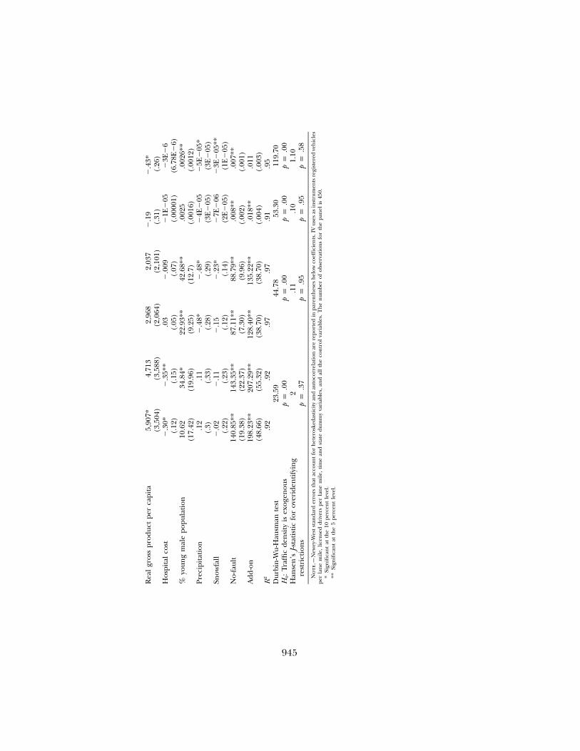
Specifications 6 and 7 in table 3 give OLS and IV estimates of ourquadratic density model (eq. [2]) using insurer costs per vehicle as thedependent variable. Specifications 8 and 9 use insurance premiums pervehicle as the dependent variable.
Both the OLS and IV specifications in table 3 reveal the same pattern.In particular, the density coefficient becomes negative (mostly insignif-icant) and the density squared coefficient positive and significant. Thesetwo effects balance to make the effect of increases in density on insur-ance rates small and of indeterminate sign in low-traffic states. The effectis positive, substantial, and statistically significant in high-traffic states,since the quadratic term dominates.
Taken together, our regressions provide strong evidence that trafficdensity increases the risk of driving. All our specifications indicate thathigh–traffic density states have very high accident costs and commen-surately large external marginal costs not borne by the driver or hisinsurance carrier. The quadratic specifications imply that the effects ofdensity increase at higher density. Congestion may eventually lower theexternal marginal accident costs, but any such effect appears to be athigher density levels than observed in our sample. Belmont (1953) in-dicates that crash rates fall only when roads have more than 650 vehiclesper lane per hour, which corresponds to nearly 6 million vehicles perlane per year, a figure well above the highest average traffic density inour sample; hence it is not surprising that we have a positive coefficienton density squared.
The framework thus far, whether using insurer cost or premiums,could still suffer, however, from potential biases. These biases flow fromnormalizing insurance costs on a per vehicle basis. Although that is theway prices are quoted in the market place, accident cost per vehicle willdepend on the amount the average vehicle is driven: the more it isdriven, the higher the costs will be. If miles per vehicle in a state rise,this could drive up both traffic density and insurance premiums pervehicle without any externality effect. Hence, if we seek to interpret thedensity term as reflecting an externality, our externality estimates mightbe biased up. On the other hand, if traffic density rises because morepeople become drivers, then each person will find driving less attractiveand drive less, reducing her risk exposure. This would bias our exter-nality estimate down and could lead to a low-density coefficient estimateeven though the externality is large. Instead of simply assuming thatthese two biases perfectly offset each other, we can remove both biaseswith a new specification.
To remove the above biases, we normalize aggregate statewide pre-
948 journal of political economy
miums by vehicle miles traveled in the state (M) instead of by the num-ber of insured vehicles. Accordingly, columns 10 and 11 report estimatesof a variant of equation (2) in which we have insurer costs per vehiclemile traveled and premiums per vehicle mile traveled as our dependentvariables. This is our preferred specification because it removes thepotential biases from variations in miles traveled per vehicle. As withour other estimates, we have a positive and significant coefficient ondensity squared; the estimates are naturally much smaller in absolutevalue because once normalized by miles traveled, the left-hand-side var-iable is roughly 10"4 smaller than in the other regressions. As we see inthe next section, this specification leads to the largest estimates of theexternality effect. This suggests that the largest bias in specification 7is the downward bias from more drivers leading to less driving per driver.
V. The External Costs of Accidents
Here we compute the extent to which the typical marginal driver in-creases others’ insurance premiums or insurers’ costs in a state. Forspecifications 3 and 7, equation (4) gives the externality on a per vehiclebasis. We convert this figure to a per licensed driver basis by multiplyingby the ratio of registered vehicles to licensed drivers in a given state.The resulting figure implicitly assumes a self-insurance cost borne byuninsured drivers equal to the insurance cost of insured drivers.
We report results for three high-traffic states, three moderate-trafficstates, and three low-traffic states in table 5. Extra driving imposes largeaccident costs on others in states with high traffic density such as NewJersey, Hawaii, and California, according to our estimates. In California,for example, our estimates range from $1,725 " $817 per driver peryear in the linear model using insurer costs per vehicle as the dependentvariable to $3,239 " $1,068 per driver in the quadratic model usinginsurer costs per mile as the dependent variable. This external marginalcost is in addition to the already substantial internalized cost of $744in premiums that an average driver paid in 1996 for liability and collisioncoverage in California.
We find that high–traffic density states such as California have largeeconomically and statistically significant externalities across all specifi-cations whether using OLS or IV, whether controlling for serial corre-lation or not controlling, whether using insurer costs or premiums asa measure, whether normalizing by vehicle miles traveled or by numberof vehicles, whether using panel or cross-sectional data, and whetherusing linear or quadratic costs. In contrast, low–traffic density stateshave small economically insignificant and generally statistically insig-nificant externalities in our estimation: in South Dakota, for example,
TAB
LE5
Year
lyE
xter
nal
Acc
iden
tC
ost
ofM
argi
nal
Dri
ver
for
Sele
ctSt
ates
,199
6
Stat
e
Traf
ficD
ensi
ty(1
996)
(1)
Insu
ranc
ePr
emiu
m,r
($/I
nsur
edC
ar-Y
ear)
(2)
Line
arIn
sure
rC
osts
per
Vehi
cle
Mod
el(B
ased
onSp
ecifi
catio
n3)
(3)
Qua
drat
icIn
sure
rC
osts
per
Vehi
cle
Mod
el(B
ased
onSp
ecifi
catio
n7)
(4)
Qua
drat
icIn
sure
rC
osts
per
Vehi
cle
Mile
Mod
el(B
ased
onSp
ecifi
catio
n10
)(5
)
Qua
drat
icIn
sura
nce
Prem
ium
spe
rVe
hicl
eM
ileM
odel
(Bas
edon
Spec
ifica
tion
11)
(6)
Low
-Den
sity
Stat
es
Nor
thD
akot
a38
,355
363
110
(52)
"46
(50)
10(4
1)"
14(3
1)So
uth
Dak
ota
46,2
7641
312
7(6
0)"
50(5
7)14
(49)
"15
(37)
Mon
tana
66,3
0445
121
4(1
01)
"73
(94)
32(7
5)"
16(5
6)
Mod
erat
e-D
ensi
tySt
ates
Mai
ne27
7,81
646
357
9(2
74)
126
(215
)50
2(2
63)
250
(161
)K
entu
cky
280,
899
604
561
(266
)12
7(2
08)
581
(302
)29
1(1
84)
Sout
hC
arol
ina
295,
083
595
608
(288
)16
0(2
24)
598
(298
)59
8(1
79)
Hig
h-D
ensi
tySt
ates
Cal
iforn
ia72
8,97
474
41,
725
(817
)2,
432
(764
)3,
239
(1,0
68)
2,23
1(6
28)
New
Jers
ey80
2,82
81,
091
1,61
9(7
67)
2,59
9(7
75)
3,25
0(1
,065
)2,
273
(639
)H
awai
i89
9,51
899
01,
831
(867
)3,
408
(973
)3,
933
(1,2
87)
2,79
6(7
91)
Not
e.—
Entr
ies
for
exte
rnal
acci
dent
cost
inco
ls.3
–6ar
ein
dolla
rspe
rdr
iver
.Sta
ndar
der
rors
are
inpa
rent
hese
s.Ex
tern
alm
argi
nalc
ost
ofad
ditio
nald
rive
ris
calc
ulat
edfr
omth
eco
stpe
rm
ileas
sum
ing
that
adr
iver
driv
esth
eav
erag
enu
mbe
rof
mile
sin
the
stat
e.
950 journal of political economy
a state with roughly one-fifteenth the traffic density of California, ourexternality estimates range from "$50 " $57 to $127 " $60.
As a comparative matter, external marginal costs in high–traffic den-sity states are much larger than either insurance costs or gasoline ex-penditures. The point estimates of the external costs are quite largeeven in moderate-density states such as Kentucky, especially in the linearmodel, where the estimate in Kentucky, for example, is $561 " $266.
Although our external cost estimates are large in high-density statessuch as New Jersey, California, and Hawaii, they are not unreasonablyso. Consider that, nationally, there are nearly three drivers involved percrash on average. According to the accident model in Section II, thiswould suggest that the marginal accident cost of driving would typicallybe three times the average and that the external marginal cost wouldbe twice the average. Hence, we might expect that a 1 percent increasein driving could raise costs by 3 percent.5 In California, a 1 percentincrease in driving raises insurer costs by roughly 3.3 percent accordingto specification 3, our linear model, and by 5.4 percent according tospecification 10. The linear model suggests that in almost all states a 1percent increase in driving raises accident costs by substantially morethan 1 percent.
Although we chose insurance loss costs and premiums because theyimplicitly include both crash frequency and crash severity effects, it isinteresting to decompose these two effects. When we do so, our pointestimates suggest that increases in traffic density appear to consistentlyincrease accident frequency, but not severity. The severity of accidentsmay fall somewhat with increases in density in low-density states and risein high-density states. However, both the severity externality and thefrequency externality are statistically insignificant, and it is only whenthe two externalities are combined (as they should be) that we uncoverstatistically significant externalities.6
VI. Implications
We find substantial negative accident externalities in almost all speci-fications, even in states with only moderate traffic density such as Ken-tucky or South Carolina; and in all specifications, the externalities areat least somewhat negative for states of moderate or higher traffic den-
5 If accidents require the coincidence of three cars in the same place at the same time,then and external marginal costs equal . Internalized marginal costs are2 2r p c D 2c D3 3
, so that total marginal cost is . If there were no external marginal costs, then a2 2c D 3c D3 3
1 percent increase in driving would increase costs by 1 percent (the internalized figure).6 For details on this decomposition, see Edlin and Karaca-Mandic (2003). There, we
also studied the fatalities externality, which is largely uninsured. As with the measures ofinsured costs studied here, our point estimates suggest that in high-density states increasesin density raise fatality rates; however, this effect is not statistically significant.
accident externality from driving 951
sity. By way of comparison, our point estimates exceeded existing taxeson gasoline in such states; externalities appear to dwarf existing taxesin states with high traffic density such as California in all specifications.The failure to charge for accident externalities provides the incentivefor too much driving and too many accidents, at least from the stand-point of economic efficiency.
The true extent of accident externalities probably substantially ex-ceeds our estimates because we neglected two important categories oflosses. In particular, we did not include the costs of traffic delays fol-lowing accidents, nor did we include damages in accidents when theselosses are not covered by insurance. Both omissions could be quitesubstantial. According to one fairly comprehensive study by the UrbanInstitute (Miller et al. 1991), the total cost of accidents (excluding con-gestion) exceeded $350 billion per year, substantially more than theroughly $100 billion per year of insured accident costs during our sam-ple period. If these uninsured accident costs behave like the insuredcosts we have studied, then accident externalities could be 3.5 times aslarge as we have estimated here. Externalities for California might ex-ceed $10,000 per driver per year.
One potential solution would be to engage in a massive road-buildingcampaign to lower traffic density. Road building is unlikely to be theanswer, however. California, for example, would need to more thandouble its road infrastructure to get its density down to Kentucky levels,and it would still have substantial externalities. Moreover, if the newroads lead to more driving, even less would be gained.
The straightforward way to address large external marginal costs isto levy a substantial Pigouvian charge, either per mile, per driver, orper gallon, so that people pay something closer to the true social coststhat they impose when they drive.7 An alternative tax base is insurancepremiums (coupled with getting very serious about requirements to befully insured).
Pigouvian taxes could rectify the externality problem and raise sig-nificant funds. If each state charged our estimated external marginalcost as a Pigouvian tax for each mile driven or each new driver, thetotal national revenue would be $220 billion per year at the end of oursample, 1996, according to the estimates in specification 10, and ne-glecting the resulting reductions in driving. This figure exceeds the $163billion collected in 1996 by all states combined for corporate and in-dividual income taxes. In California alone, revenues would be $66 bil-lion, more than the $57 billion for all California state tax collections.New Jersey, another high-traffic state, could likewise gather more rev-
7 In principle, accident charges should vary by roadway and time of day to account forchanges in traffic density.
952 journal of political economy
enue from an appropriate accident externality tax than it does from allits state taxes: $18 billion compared to $14 billion in 1996.8 If uninsuredexternality costs are in fact 3.5 times insurance costs, as suggested bythe Urban Institute study, then an appropriate Pigouvian tax might raise$770 billion per year before accounting for what would in fact be enor-mous driving reductions. That quantity is a shockingly large figure, butone that reflects the magnitude of the problem. Of course, the numberof drivers and the amount of driving would decline significantly withsuch a tax, and that would be the point of the tax, because less drivingwould result in fewer accidents.
The most administratively expedient Pigouvian tax would be a gas-oline tax since states already have such taxes. And, importantly, gas taxeswould bring the uninsured into the payment system. On the negativeside, such taxes take inadequate account of heterogeneity. Good andbad drivers are charged the same amount, even though the accidentfrequency and hence the accident externality of bad drivers could beconsiderably higher. In addition, fuel-efficient vehicles would pay loweraccident externality fees, even if they impose comparable accident costs.
In principle, the most efficient way to address the accident externalitywould probably be to levy a large tax on insurance premiums. A tax oninsurance premiums, unlike a gas tax, would take into account hetero-geneity because insurance premiums already do so. In California, aPigouvian tax might be roughly 200–400 percent, as revealed in table5. A practical difficulty with taxing insurance is that it would drive peopleto become uninsured unless states simultaneously cracked down seri-ously on uninsured driving.
To an economist, raising significant funds with Pigouvian taxes onexternalities is a dream come true. Many political watchers will doubt,though, that Americans will accept any policy that substantially raisesthe cost of driving. Gasoline taxes, for example, remain quite low inthe United States compared with Europe.
Surprisingly, there is a potential second-best compromise, which is toshift a fixed cost to the margin, so as to leave overall driving costscomparable, but increase the marginal cost and thereby decrease thequantity of driving. The body politic has accepted mandatory insurance,so why not also require insurance companies to quote premiums by themile instead of per car per year? Insurance premiums are surprisingly
8 Tax figures are available from the Census Bureau, 1996 State Government Tax Collections(http://www.census.gov/govs/www/statetax96.html).
accident externality from driving 953
invariant to the amount a given individual drives,9 and as a result, onceone buys a car and insurance, the price of gasoline alone becomes thelimiting factor on quantity of driving.
Why not instead have “per mile premiums,” much as William Vickrey(1968) once suggested, in which insurance charges rise linearly with anindividual’s driving. This simple change in pricing structure could re-duce driving substantially by moving a fixed cost to the margin withoutraising the overall cost of driving. Litman (1997) and Edlin (2003)provide more extensive discussions of this possibility.10 People couldthen choose to save substantial amounts on insurance by reducing theirdriving. As driving distributions are skewed, most people drive less thanthe average (and so would save money under per mile premiums). Thisfact makes the political prospects of such a change seem more promisingthan a tax that would raise overall driving costs. The National Orga-nization for Women, Butler, Butler, and Williams (1988), and Butler(1990) have argued forcefully that such a policy would be more fair aswell, pointing out that women drive roughly half what men do, havehalf the accidents, but still pay comparable premiums (see also Ayresand Nalebuff 2003).
An extremely valuable aspect of a requirement of per mile premiumsis that it takes advantage of the fact that current insurance premiumsaccount for heterogeneity in risk. As a result, those in highly dense areasand those with poor driving records would face the highest per milerates and would reduce driving the most, creating a doubly large re-duction in accidents—exactly as a social planner would wish.
Edlin (2003) estimated that the accident savings net of lost drivingbenefits from per mile premiums would be $12.7 billion per year na-tionwide. Those estimates were, however, based on a simulation modelof accident externalities that assumed a much lower accident externalitythan the one estimated here, suggesting that the actual gains would beconsiderably larger.
9 For example, State Farm, the largest U.S. insurer, distinguishes in most states on thebasis of whether a driver predicts driving under or over 7,500 miles annually and grants15 percent discounts to drivers who drive under 7,500 miles. This discount is modest giventhat those who drive under 7,500 miles per year average 3,600 miles compared to 13,000for those who drive over 7,500 according to our calculations from the 1994 ResidentialTransportation Energy Survey of the Department of Energy Information Administration.The implied elasticity of accident costs with respect to miles is 0.05, an order of magnitudebelow what the evidence suggests is the private elasticity of accident costs with respect todriving. The link between driving quantity and premiums may be attenuated in partbecause there is significant noise in self-reported estimates of future mileage, estimateswhose accuracy does not affect insurance payouts.
10 Several firms, such as Norwich-Union, a British insurer, have begun experimentingwith various types of “pay as you drive insurance.” See http://news.bbc.co.uk/hi/englishbusiness/newsid-1831000/1831181.stm and http://www.norwich-union.co.uk for infor-mation on Norwich-Union.
954 journal of political economy
One reason that insurers do not adopt per mile premium policies ontheir own is that so much of the gains are external and the monitoringcosts are internal. Currently a firm that quotes such premium schedulesbears all the costs of monitoring mileage but gleans only a fraction ofthe benefits: as its insureds cut back their driving, others avoid accidents(with them), and these others and their insurance companies benefitconsiderably. This externality, which is exactly what we have estimated,is what suggests that regulatory intervention could be warranted. Somehave suggested that insurers might band together to adopt per milepremiums without regulation, but there is little incentive to do that(even if it were not illegal price fixing) since they would compete awayany gains.
To conclude, substantially more research on accident externalitiesfrom driving seems appropriate, particularly given the apparent size ofthe external costs. There is substantial heterogeneity within states intraffic density, so more refined data (such as county-level data or time-of-day data) would yield more accurate estimates of the effect of trafficdensity and correspondingly of external marginal costs. In principle, itwould also be instructive to disaggregate traffic density into its com-ponents by the age of the driver and by vehicle type. Likewise, it wouldbe instructive to study micro-level data correlating the number of ve-hicles involved in the average accident with accident costs and frequency.
References
Ayres, Ian, and Barry Nalebuff. 2003. “Make Car Insurance Fairer.” Forbes 171(March 17): 54.
Belmont, D. M. 1953. “Effect of Average Speed and Volume on Motor-VehicleAccidents on Two-Lane Tangents.” Proc. Highway Res. Board 32: 385–95.
Butler, Patrick M. 1990. “Measure Exposure for Premium Credibility.” Nat. Un-derwriter 94 (April 23): 12.
Butler, Patrick M., Twiss Butler, and Laurie L. Williams. 1988. “Sex-Divided Mile-age, Accident, and Insurance Cost Data Show That Auto Insurers OverchargeMost Women.” J. Insurance Regulation 6 (March): 243–84.
Cooter, Robert, and Thomas Ulen. 1988. “You Can’t Kill Two Birds with OneStone.” In Law and Economics. Glenview, IL: Scott Foresman.
Edlin, Aaron S. 2003. “Per-Mile Premiums for Auto Insurance.” In Economics foran Imperfect World: Essays in Honor of Joseph E. Stiglitz, edited by Richard Arnott,Bruce Greenwald, Ravi Kanbur, and Barry Nalebuff. Cambridge, MA: MITPress.
Edlin, Aaron S., and Pinar Karaca-Mandic. 2003. “The Accident Externality fromDriving.” Working Paper no. E03-332, Univ. California, Berkeley, Dept. Econ.
Green, Jerry. 1976. “On the Optimal Structure of Liability Laws.” Bell J. Econ. 7(Autumn): 553–74.
Insurance Information Institute. 1998. Fact Book. New York: Insurance Infor-mation Inst.
Insurance Research Council. 1995. Trends in Auto Injury Claims. Wheaton, IL:Insurance Res. Council.
accident externality from driving 955
Levitt, Steven D., and Jack Porter. 2001. “How Dangerous Are Drinking Drivers?”J.P.E. 109 (December): 1198–1237.
Litman, Todd. 1997. “Distance-Based Vehicle Insurance as a TDM Strategy.”Transportation Q. 51 (Summer): 119–37.
Lundy, Richard A. 1965. “Effect of Traffic Volumes and Number of Lanes onFreeway Accident Rates.” Highway Res. Record 99: 138–56.
Miller, Ted R., Shelli G. Rossman, and John Viner. 1991. The Costs of HighwayCrashes: The Final Report. Washington, DC: Urban Inst.
National Association of Insurance Commissioners. Various years. State AverageExpenditures and Premiums for Personal Automobile Insurance. Kansas City: NAICPublications Dept.
Newey, Whitney K., and West, Kenneth D. 1987. “A Simple, Positive Semi-definite,Heteroskedasticity and Autocorrelation Consistent Covariance Matrix.” Econ-ometrica 55 (May): 703–8.
Shavell, Steven. 1980. “Liability versus Negligence.” J. Legal Studies 9 (January):1–25.
Turner, D. J., and R. Thomas. 1986. “Motorway Accidents: An Examination ofAccident Totals, Rates and Severity and Their Relationship with Traffic Flow.”Traffic Engineering and Control 27 (July/August): 377–83.
U.S. Department of Transportation, National Highway Traffic Safety Adminis-tration. 1996. Traffic Safety Facts: A Compilation of Motor Vehicle Crash Data fromthe Fatality Analysis Reporting System and the General Estimates System. Washington,DC: U.S. Government Printing Office.
Vickrey, William. 1968. “Automobile Accidents, Tort Law, Externalities, and In-surance: An Economist’s Critique.” Law and Contemporary Problems 33 (Sum-mer): 464–87.
Wood, Richard A. 1999. Weather Almanac: A Reference Guide to Weather, Climate,and Related Issues in the United States and Its Key Cities. 9th ed. Detroit: GaleGroup.