The Advanced Regional Prediction System (ARPS) - A multi-scale nonhydrostatic atmospheric simulation and prediction model. Part I: Model Dynamics and Verification

Ming Xue1,2, Kelvin K. Droegemeier1,2 and Vince Wong1

1Center for Analysis and Prediction of Storms

2 School of Meteorology

University of Oklahoma

Norman OK 73019

Submitted to Meteorology and Atmospheric Physics

March, 2000

Minor changes June 2000

Accepted June 2000

Corresponding Author Address: Dr. Ming Xue, School of Meteorology, University of Oklahoma,

Sarkeys Energy Center, Suite 1110, 100 East Boyd, Norman, OK 73019. E-mail: mxue@ou.edu.

Summary

A completely new nonhydrostatic model system known as the Advanced Regional Prediction System (ARPS) has been developed in recent years at the Center for Analysis and

Prediction of Storms (CAPS) at the University of Oklahoma. The ARPS is designed from the

beginning to serve as an effective tool for basic and applied research and as a system suitable for explicit prediction of convective storms as well as weather systems at other scales. The ARPS

includes its own data ingest, quality control and objective analysis packages, a data assimilation

system which includes single-Doppler velocity and thermodynamic retrieval algorithms, the forward

prediction component, and a self-contained post-processing, diagnostic and verification package. The forward prediction component of the ARPS is a three-dimensional, nonhydrostatic

compressible model formulated in generalized terrain-following coordinates. Minimum

approximations are made to the original governing equations. The split-explicit scheme is used to

integrate the sound-wave containing equations, which allows the horizontal domain-decomposition

strategy to be efficiently implemented for distributed-memory massively parallel computers. The

model performs equally well on conventional shared-memory scalar and vector processors. The

model employs advanced numerical techniques, including monotonic advection schemes for scalar transport and variance-conserving fourth-order advection for other variables. The model also

includes state-of-the-art physics parameterization schemes that are important for explicit prediction

of convective storms as well as the prediction of flows at larger scales. Unique to this system are the consistent code styling maintained for the entire model system

and thorough internal documentation. Modern software engineering practices are employed to

ensure the system is modular, extensible and easy to use. The system has been undergoing real-time prediction tests at the synoptic through storm

scales in the past several years over the continental United States as well as in part of Asia, some of which included retrieved Doppler radar data and hydrometeor types in the initial condition.

As the first of a two-part paper series, we describe herein the dynamic and numerical framework of the model, together with the subgrid-scale turbulence and the PBL parameterization. The model dynamic and numerical framework is then verified using idealized and realistic mountain

flow cases and an idealized density current. Other physics parameterization schemes will be

described in Part II, which is followed by the verification against observational data of the coupled

soil-vegetation model, surface layer fluxes and the PBL parameterization. Applications of the model to the simulation of an observed supercell storm and to the prediction of a real case are also found in

Part II. In the latter case, a long-lasting squall line developed and propagated across the eastern part of the United States following a history number of tornado outbreak in the state of Arkansas.

1

1. Introduction

Three-dimensional nonhydrostatic modeling of atmospheric convection started in the mid-1970s (e.g., Steiner, 1973; Miller and Pearce, 1974; Schlesinger, 1975; Tapp and White, 1976; Clark, 1977; Klemp and Wilhelmson, 1978), following the success of earlier 2-D modeling studies

that used nonhydrostatic equations in either primitive form (Lilly, 1962) or vorticity form (Orville, 1968). These and other studies significantly advanced our understanding of thunderstorm dynamics

(Lilly, 1979; Klemp, 1987) as well as other small-scale phenomena. However, modeling research

on the storm-scale (defined here loosely as the scale at which non-hydrostatic dynamics are

important and attention is paid to individual storm elements, e.g., updrafts and downdrafts) remained in the simulation mode for much of the last two decades. These simulations typically used

horizontally homogeneous initial conditions with artificial perturbations to initiate convection. Two major developments in the recent years provided the impetus for moving from a mode

of convective storm simulation to one of prediction. The first is the deployment of about 160

Doppler radars (Crum and Albert, 1993) in the U. S. that provides nearly continuous single-Doppler coverage of spatial and temporal scales relevant to storm prediction. The second concerns with

techniques for retrieving unobserved quantities from single-Doppler radar data to yield a consistent set of mass and wind fields appropriate for initializing a storm-scale prediction model (e.g., Kapitza, 1991; Liou et al., 1991; Sun et al., 1991; Qiu and Xu., 1992; Shapiro et al., 1995; Sun and Crook, 1994). Perhaps equally important for the realization of numerical weather prediction (NWP) on the

storm scale is the advent and accessibility of increasingly more powerful parallel-processing

supercomputers. In 1989, the Center for Analysis and Prediction of Storms was established at the University

of Oklahoma as one of the National Science Foundation’s first 11 Science and Technology (S&T) Centers. Its formal mission is to demonstrate the practicability of storm-scale numerical weather

prediction and to develop, test, and validate a regional forecast system appropriate for operational, commercial, and research applications. Its ultimate vision is to make available a fully functioning

stormscale NWP system around the turn of the century (Lilly, 1990; Droegemeier, 1990). Central to achieving this goal is an entirely new three-dimensional, nonhydrostatic model system known as the Advanced Regional Prediction System (ARPS). It includes a data ingest, quality control, and objective analysis package, a single-Doppler radar parameter retrieval and

assimilation system, the prediction model itself, and a post-processing package. These components

are illustrated in Fig. 1. In planning for its development, the ARPS was required to meet a number of criteria. First, it had to accommodate, through various assimilation strategies, new data of higher temporal and

spatial density (e.g., WSR-88D data) than had traditionally been available. Second, the model had to

serve as an effective tool for studying the dynamics and predictability of storm-scale weather in both

idealized and more realistic settings. It must also handle atmospheric phenomena ranging from

regional scales down to micro-scales as interactions across this spectrum are known to have

profound impacts on storm-scale phenomena. These needs required that the model have a flexible

and general dynamic framework and include comprehensive physical processes. The system should

also run efficiently on massively parallel computers. In short, it was our goal to develop a model system that can be used effectively for both basic atmospheric research and operational numerical weather prediction, on scales ranging from regional to micro-scales. In section 2 of this paper, we will describe the dynamic framework of the forward prediction

component of the ARPS system. We will describe in section 3 several options of subgrid-scale

turbulence parameterization together with a 1.5-order turbulent kinetic energy (TKE)-based

2

planetary boundary layer (PBL) parameterization scheme. Other physics parameterizations will be

detailed in Part II (Xue et al., 2000) and will be briefly outlined in section 4. The numerical treatment of various processes in the model is presented in section 5 with additional details found in

the Appendices. Section 6 discusses the computational aspects of the model, and Sections 7 and 8

verify the dry dynamics of the model using mountain flows and a nonlinear density current. Summary is found in section 9.

2. Dynamics Equations

2.1. Historical perspective

Three-dimensional nonhydrostatic models can be divided into two broad categories: those

containing fast acoustic modes (Tapp and White, 1976; Klemp and Wilhelmson, 1978, KW

hereafter) and those that filter such modes via certain type of anelastic approximation (Miller and

Pearce, 1974; Schlesinger, 1975; Clark, 1977; Xue and Thorpe, 1991). For the former, commonly

referred to as compressible models, the acoustic waves must be treated in special ways to attain

computational efficiency. Tapp and White (1976) used a semi-implicit integration scheme that is

absolutely stable for linearized sound waves, while Klemp and Wilhelmson (1978) employed a

mode-splitting technique where the acoustic waves and slow modes are integrated separately using

different time steps. In the latter case, the vertical acoustic modes are usually treated implicitly to

remove the time step limitation from these modes due to the Courant-Fredrichs-Lewy (CFL) stability condition.

In the anelastic (sound-proof) models, a prognostic equation for pressure (or alternatively

density) is absent, and the pressure (or geopotential height in pressure-based coordinates) has to be

diagnosed from an elliptic equation derived from the equations of motion. In order to filter out acoustic modes, certain approximations have to be made (see, e.g., discussion by Durran, 1989).

The mode-splitting technique has gained considerable popularity since KW because of its

simplicity and effectiveness (Tripoli and Cotton, 1982; Chen, 1991; Tripoli, 1992; Dudhia, 1993; Hodur, 1997). An attractive feature of models using this approach is that all computations are local to the grid points involved in the finite difference stencil, making their implementation on

distributed-memory parallel processor (PP) computers straightforward through the use of domain

decomposition strategies (Johnson et al., 1994; Droegemeier et al., 1995b). Different from anelastic

systems, the compressible system of equations does not have to make any approximation, making it suitable to a wider range of applications. The semi-implicit method used by Tapp and White (Tapp and White, 1976) for compressible

systems has in recent years been adopted by other models (Tanguay et al., 1990), and has been

further extended to include linear gravity wave modes (Cullen, 1990) so as to remove its time step

limitation. Because of its absolute stability with respect to modes treated implicitly, this method is

often combined with semi-Lagrangian advection schemes (Tanguay et al., 1990; Golding, 1990) to

achieve high computational efficiency. In practice, however, the efficiency of such schemes has to

be considered together with solution accuracy. For example, it is known that implicit schemes

distort (slow down) gravity waves when used with large time steps (Tapp and White, 1976). Semi-implicit systems usually involve solving a global elliptic equation, making their efficient implementation on distributed-memory parallel computers less straightforward.

Based on the above considerations, we choose to use a fully compressible system of equations and solve them using the ‘split-explicit’ time integration method.

3

2.2. The governing equations of ARPS

The governing equations of the ARPS include conservation equations for momentum, heat, mass, water substance (water vapor, liquid and ice), subgrid scale (SGS) turbulent kinetic energy

(TKE), and the equation of state of moist air. Among the three state variables, i.e., temperature, pressure and density, prognostic equations for two of them are needed and the third variable can be

diagnosed from the equation of state. For the temperature, modelers usually choose between temperature (e.g., Dudhia, 1993), and

potential temperature(e.g., KW). Some modelers favor ice-liquid potential temperature (e.g., Tripoli and Cotton, 1981). In the ARPS, we choose to predict potential temperature and pressure then

diagnose density. The potential temperature is chosen because it is conservative for adiabatic

processes. The ice-liquid potential temperature is supposed to be conserved even in the presence of phase changes, but its definition involves approximations.

For the pressure equation, modelers again have the choice of using pressure or Exner function as the prognostic variable. Most existing compressible models predict the Exner function

instead of pressure (e.g., Klemp and Wilhelmson, 1978; Tapp and White, 1976), but we choose to

predict pressure. In such a case, the pressure gradient force (PGF) is written as in the original Navier-Stokes equations (e.g., Batchelor, 1967), so that a fully conservative form of the momentum

(not velocity) equations can be formulated, both analytically and numerically. The ARPS governing equations are first written in a Cartesian coordinate projected onto a

plane tangent to or intercepting the earth's surface. Using standard mathematical relations (Haltiner and Williams, 1980) for the transformation from a local Cartesian space on the sphere to map

projection space, we obtain the following equations of motion:

1 1( )x m uu mp f f v f w uwa Fρ − −= − + + − − + , (1a)

1 1( )y m vv m p f f u vwa Fρ − −= − − + − + , (1b)

1 2 2 1( )z ww p g f u u v a Fρ − −= − − + + + + . (1c)

In the above and in the equations to follow, the dot operator denotes the total time derivative, e.g., /u du dt , and subscripts t, , , , , and x y z ξ η ζ denote partial temporal or spatial derivative, e.g., u u xx / . In obtaining (1a-c), no approximation is made other than that the ellipticity of the earth

is neglected and the atmosphere is assumed to be thin so that the radius is replaced by the mean

earth radius at the sea level a. Note that the spatial derivatives of map factor due to curvature are

retained in tan( ) /m y xf um vm u aφ≡ − + , as are the Coriolis terms due to vertical motion (those

involving

~f ). The definitions of other symbols are found in Appendix A. Note that for this system,

only gravitational, pressure gradient and frictional forces (F terms) can change kinetic energy. All other terms cancel each other in the kinetic energy equation. The equations of state for moist air (see Dutton, 1986), mass continuity, heat energy

conservation, and conservation of hydrometeor species are, respectively,

1 1( ) 1 ( ) (1 )d v v v lip R T q q q qρ ε− − = − + + + , (1d)

2 ( / ) ( / )x y zm u m v m wρ ρ = − + + , (1e)

1( )pQ Cθ π −= , (1f)

q Sq . (1g)

Here Q denotes heat source, and Sq represents sources due to moist processes.

4

2.3. The curvilinear coordinate system

The actual equations of the ARPS are written in a curvilinear coordinate system (ξ, η, ζ) defined by

( ), ( ), ( , , )x y x y zand . (2) This coordinate system is a special case of the fully three-dimensional curvilinear system since

constant surfaces of ξ and η remain parallel to those of constant x and y, respectively. The vertical transformation allows grid stretching and ensures that the lower boundary conforms to the terrain. The horizontal transformation allows horizontal grid stretching. Eqs.(2) represent a transformation

that maps a domain with stretched grid and irregular lower boundary to a regular rectangular domain

with equal grid space in each direction. We call the latter the computational domain. The governing equations for fluid motion in a fully 3-D curvilinear system can be found in

Thompson et al. (1985), Sharman et al. (1988) and Shyy and Vu (1991). Following their work, we

use the Cartesian instead of the contravariant velocity components as the basic dependent variables. As shown in Sharman et al. (1988), the Cartesian velocity components u, v and w can be expressed

as functions of the contravariant velocities Uc, Vc and Wc

and vice versa. For the transformation

defined by (2), which is a special case of the fully 3-D curvilinear transformation, we have

U uJ G u xc 3 / / , V vJ G v yc

4 / / , and W uJ vJ w x y Gc ( ) / ,1 2 (3)

where

J z y J z x J z y J z x1 2 3 4 , , , and G z x y . (4)

J J J J1 2 3 4, , and are Jacobians of transformation and G is the determinant of the Jacobian matrix

of transformation from the (ξ, η, ζ) system to the (x, y, z) system. It is clear that Uc differs from u by

a factor of xξ, which is the grid stretching factor in the x-direction. The same is true in the y

direction. The formula for Wc is more complicated because this component is not orthogonal to the

other velocity components. The transformation relations for spatial derivatives from (x,y,z) to (ξ, η, ζ) coordinates are

x J J G 3 1b g b g / ,

y J J G 4 2b g b g / , and z x y G d i / . (5)

Most terrain-following coordinate models (e.g., Clark, 1977; Pielke and Martin, 1981) define the coordinate transform therefore the transformation Jacobians analytically. In the ARPS, the computational grid is defined numerically and therefore can be arbitrary. The Jacobians are

calculated numerically according to (4). This allows for additional flexibility, in fact, the grid can be

made time dependent (Fiedler et al., 1998). The only requirement for the grid generation is that the

lowest grid level conforms to the terrain. Several built-in options for creating the computational grid

with optional stretching are available in the model. They allow for easy setup of, for example, quasi-uniform vertical levels at the lower and upper levels, and stretched levels in-between. One can also

choose to flatten the coordinate surfaces above a certain height, so that the error associated with

calculating horizontal gradients (e.g., in horizontal PGF terms) in a non-orthogonal grid is

eliminated there. Fig. 3 shows an example of this generalized terrain-following coordinate in which

the vertical grid is stretched and the coordinate levels become flat at a given height.

2.4. Final Model Equations

Following the practice of most non-hydrostatic atmospheric models (e.g., Clark, 1977; Dudhia, 1993), we divide the atmospheric state variables into the base-state (reference state) and the

deviation

( ) 'z .

5

The base-state is intentionally chosen to be independent of x and y so that explicit evaluation of its

horizontal gradient in the (ξ, η, ζ) coordinate is avoided. This eliminates the usually large

cancellation errors associated with such calculations. The need to solve the perturbation equations

for vertical acoustic waves implicitly is another reason for defining the reference state. As will be

seen later, as long as we retain high-order perturbation terms, the actual choice of the base state has

little effect on the final solution. The base state is required to satisfy the hydrostatic relation: p gz , (6)

where is the base-state density that contains the effect of base-state water vapor. For convenience of notation, we define the following:

* * * * * * *, , G U U V V W Wc c cand . (7)

The final prognostic equations in the ARPS are obtained by transforming Eqs.(1a-g) into the

curvilinear coordinate using relations given in the previous section. In addition, there is an equation

for the sub-grid scale turbulent kinetic energy (TKE) E:

( )

* 1 * *3 1

* 1

( ) ( ' ) ( ' )

( ) ,

t

m u

u m J p Div J p Div

ADV u f f v f w uwa GD

ξ ξξ ζρ ρ ρ α α

ρ

−

−

+ − + − =

− + + − − +

(8a)

( ) * 1 * *4 2

* 1

( ' ) ( ' )

( ) ( ) ,

t

m v

v m J p Div J p Div

ADV v f f u vwa GD

η ηη ζρ ρ ρ α α

ρ

−

−

+ − + − =

− − + − + (8b)

( ) ( ) 1* 1 * 1 * 1

1 * * 2 2 1

( ' ) ' '

( ) ' ( ) ,

t

w

w x y p Div g p p

ADV w g B f u u v a GD

ξ η ζ ζρ ρρ α ρρ ρ γ θ θ

ρρ ρ ρ

−− − −

− −

+ − + − =

− + + + + +

(8c)

( ) ( ) ( ) ( )

2 2 1 1

2 1 1

'

' ' ' ,

c c cs

t

c c cs

G p G gw c m GU m GV m GW

m GU p GV p GW p G c AA

ξ η ζ

ξ η ζ

ρ ρ

ρ θ θ

− −

− −

− + + + =

− + + + +

(8d)

* *' ( ' )c ht xw ADV GD GS (8e)

* *( ) /q ADV q V q z GD GSt q q qc h d i , (8f)

* * * /( ) /E ADV E C K Def E Div C l E GDt m Ec h

2 1 3 22 3 2 (8g)

where the advection operator ADV(φ) is defined as

( ) ( ) ( )

* * *

2 * 1 * 1 * *

( )ADV m U V W

m U m V m W G Div

ξ η ζ

ξ η ζ

φ φ φ φ

φ φ φ φ− −

≡ + +

= + + −

(9)

and the density weighted divergence Div* is defined as

( ) ( ) * 2 * 1 * 1 *( ) 1/Div V G m U m V m W ζξ η

ρ − − ≡ ∇ ⋅ = + +

. (10)

2.5. Discussion of the Equations

In vertical momentum equation (8c), B' includes the contributions of water species and

second order perturbation pressure and temperature to the buoyancy:

6

Bq

q

q q

q

p

p

p

pv

v

v li

v

'' ' ' ' ' '

1

1

2 2

2

2 2

2

2. (11)

Retaining the second-order terms minimizes the impact of approximations due to expansions around

the reference state. Neglecting terms of orders higher than second order in (11) is the only

approximation made from equation set (1) to (8). Terms D in the equations denote subgrid scale

turbulence and computational mixing/numerical diffusion, while most other terms are readily

recognizable. It should also be noted that in the horizontal PGF and other terms where the horizontal

gradient of base-state variables is taken, we explicitly set these terms to zero. By doing so, we avoid

potentially large cancellation error associated with computing horizontal finite differences in the

transformed coordinate. This problem becomes particularly serious when the atmosphere is strongly

stratified in the vertical and the horizontal grid spacing is much larger than the vertical (Janjic, 1977; Mesinger and Janjic, 1985). By separating the horizontally homogeneous base-state from the

total state variables (which is not typically done in hydrostatic models) and explicitly setting their horizontal gradients to zero, the numerical accuracy of the model is improved. The use of flattened

coordinate surfaces at the upper levels, as mentioned earlier, also helps reduce such cancellation

errors, particularly near the tropopause where the vertical change in stratification is large. In Eq.(8c), the hydrostatically balanced portion of the vertical pressure gradient is subtracted

off, again to reduce cancellation error. The perturbation density ρ' has to be diagnosed. To facilitate

the use of vertically implicit solver for acoustic modes (discussed further later), we expand ρ' in

terms of other prognostic variables and retain all first-order terms as well as second-order terms in θ' and p', as they appear in Eq.(11). This should give sufficient accuracy for almost all meteorological applications. The terms involving α Div*

in the momentum equations are artificial “divergence damping”

terms designed to attenuate acoustic waves, where , and are the damping coefficients in

three directions (Skamarock and Klemp, 1992). By performing a divergence operation on the momentum equations, one can obtain a 3-D divergence equation of the form

Div Div Div Divt xx yy zz

* * * * ...c h c h c h c h . (12)

It is clear that these terms act to reduce small-scale mass divergence thereby damp acoustic waves. Different from Skamarock and Klemp (1992), we formulate the damping in terms of mass weighted divergence instead of velocity divergence. The inclusion of a divergence damping is, however, not always needed, especially when vertical acoustic waves are treated implicitly with the forward biasing in the time averaging.

The pressure equation (8d) is derived from equation of state (1d) and mass continuity equation (1e). The last term on the RHS of the equation include contributions to pressure change

from diabatic heating and changes in water vapor, liquid and ice water. A ≡ 1 + 0.61qv + qli. In

general, such contributions are small and Dudhia (1993) argues that a model with a rigid lid behaves more realistically (more like an atmosphere without an upper lid where the air expands isobarically) without these terms. The model has the option to neglect these terms as well. Equations (8e) and (8f) are the conservation equations for potential temperature θ and water species (qv, qc, qr, qi, qs and qh). Terms S are the sources from microphysical, radiative and other processes. Again explicit advection of and qv is avoided. The second term on the RHS of the q

equation represents hydrometer sedimentation at a terminal velocity Vq, and is non-zero for rainwater, snow and hail or grapual.

7

It should be noted that the momentum and scalar conservation equations (8a-g) have been

multiplied by on both sides. Doing so yields a set of equations whose advection terms can be

written in a flux-divergence form for anelastic flows, and can be formulated to conserve the density- ( ) weighted first and second moments of the advected quantities numerically, thereby controlling

nonlinear computational instability. Finally, since a minimum of approximations were made in equation set (8), the system

should maintain good energy conservation as does the original unapproximated set in (1).

3. Subgrid-scale and PBL turbulence

3.1. Subgrid-scale turbulence parameterization

In the ARPS, three subgrid-scale (SGS) closure options for turbulent mixing terms D in Eqs.(8a-f) are available: the first-order Smagorinsky/Lilly scheme (Smagorinsky, 1963; Lilly, 1962); the 1.5-order TKE-based scheme (Deardorff, 1980; Klemp and Wilhelmson, 1978; Moeng, 1984); and the Germano dynamic closure scheme (Germano et al., 1991; Wong, 1992; Wong and Lilly, 1994). We retain fully three dimensional formulation at all scales and include the map factor, m, in the formulation. According to Smagorinsky (1963) and Lilly (1962), the turbulent terms represented by D in

the momentum equations (8a-c) may be expressed in terms of the Reynolds stress tensor τij,

1 2 3( ) ( ) ( )iu i x i y i zD m τ τ τ = + + , (13)

where index i (=1, 2 or 3) represents the Cartesian coordinates. The stress tensor ijτ is related to the

deformation tensor Dij through

i j mj i jK D (14)

where Km j is the turbulent mixing coefficient for momentum in the xj direction and deformation

tensor Dij is defined as

D m m m u m m u m mij i j k i j k x j i k xi j

RST

UVW/ ( ) / ( ) (15)

where iu are velocity components and m m m1 2 and m3 1 .

The turbulent mixing for θ and water variables has a general form of

D m H H Hx y z 1 2 3b g b g b g , (16)

where Hj is the turbulent flux of φ in xj direction, H K mj Hj j x j

( ) , (17)

and KHj is the corresponding mixing coefficient. In general, the same KH is used for heat, moisture

and hydrometeor quantities and is related to Km through the turbulent Prandtl number, Pr, i.e., KH

=Km / Pr. In the model, the above formulae are expressed in curvilinear coordinates (ξ, η, ζ).

a) The 1.5-order TKE-based turbulence closure

In the 1.5-order turbulence closure, the eddy mixing coefficient is related to a mixing length l and a velocity scale measured by the SGS turbulent kinetic energy (TKE), E, Kmj = 0.1 E1/2 lj . (18) Here we make prevision for using different length scales in different directions.

For isotropic turbulence, the length scale is

8

1 2 3

for unstableor neutralcase

min( , ) for stablecases

l l ll

∆= = = ∆

(19)

where ∆ = (∆x ∆y ∆z / m2 )1/3 and 1/ 2 10.76sl E N −= according to Moeng (1984).

When the horizontal grid spacing is much larger than vertical grid spacing, it becomes

necessary to use different horizontal length scale (∆h ) than in the vertical (∆v). For this case of anisotropic turbulence,

l1 = l2 = ∆h and 3

for unstableor neutralcase

min( , ) for stable casev

v s

ll

∆= ∆

. (20)

In this case, the turbulent Prandtl number is determined according to

Pr max / , /

1 3 1 2 3

1l vb g , (21)

where the lower limit of 1/3 is effective when the vertical length scale l3 exceeds the vertical grid

scale ∆v, which can occur when the TKE-based non-local PBL parameterization scheme to be

described in Section 3.2 is used. The time-dependent TKE is predicted by Eq.(8g). The equation includes terms for buoyancy and shear production, and dissipation and diffusion of TKE. The ground surface heat and moisture fluxes (to be discussed in Section 4) also directly contribute the production of turbulence. The dissipation term is related to E and length scale l while the diffusion term has a similar form as that for other scalar variables. In the dissipation term, we choose Cε = 3.9 at the lowest model level and

Cε=0.93 at the other levels after Deardorff (1980) and Moeng (1984).

b) Smagorinsky-Lilly turbulence closure

The modified Smagorinsky scheme (Smagorinsky, 1963; Lilly, 1962) relates Km to grid-scale flow deformation and static stability instead:

Km j = (k ∆j)2

[ max( |Def |2 - N 2/ Pr , 0 ) ]1/2

, (22)

where k= 0.21 after Deardorff (1972). ∆j is a measure of the grid length scale. It is clear that Km is

non-zero only when the Richardson number 2 2| |Ri N Def −≡ is less than Pr. This critical Richardson number often is defined to be a user-specified value between 1/3 and 1. |Def| is the magnitude of the deformation |Def| and N is the Brunt-Väisälä frequency calculated according to Durran and Klemp (1982) for moist air. On a model grid with similar grid spacings in all three directions, the SGS turbulence is nearly isotropic, so that ∆j = (∆x ∆y ∆z / m2 )1/3 for all j. (23) When the grid aspect ratio (∆x /∆z ) is large (e.g., for mesoscale and synoptic scale applications), we use different length scales in the horizontal and vertical, in the same way as we do with the TKE turbulence option.

c) Germano dynamic closure scheme

This scheme is the same as the Smagorinsky-Lilly scheme except that the parameter k in Eq.(22) is dynamically determined based on local flow and varies with space and time. As such, the SGS representation is adjusted to match the statistical structure of the smallest resolvable eddies. More details can be found in Germano et al. (1991), Wong (1992) and Wong and Lilly (1994). The non-terrain version of the Germano scheme is currently available for the ARPS (Wong, 1994).

9

3.2. The non-local PBL parameterization

The turbulence closure schemes discussed in Section 3.1 are designed to parameterize the local mixing due to sub-grid scale turbulence. In a convectively unstable boundary layer, most of the vertical mixing is achieved by 'large' boundary layer eddies (Wyngaard and Brost, 1984). Unless the vertical as well as the horizontal resolutions of the model are on the order of 100 m or less so as resolve most of the boundary layer eddies (100 m or less), additional parameterization is necessary. The treatment of convective boundary layer turbulence in the model is a combination of the 3-D, 1.5-order Deardorff SGS turbulence scheme discussed in Section 3.1 and an ensemble turbulence closure scheme of Sun and Chang (1986). The vertical turbulent mixing length l3 in (20) is related to the (non-local) PBL depth instead of the local vertical grid spacing inside an unstable PBL. This relationship is based on the profile of peak vertical wavelength of vertical velocity derived by Caughey et al. (1979) from observational data; that is

3 01.8 [1 exp( 4 / ) 0.0003exp(8 / )]i i il l z z z z z= − − − , (24)

where z is the height above ground and zi the top of PBL. Constant l0 is chosen to be 0.25. In our implementation, zi is defined as the height at which a parcel lifted from the surface layer becomes

neutrally buoyant. Under stable conditions or above the convective boundary layer, the length scale l reverts back to that of the Deardorff scheme as in (19) or (20). The performance of this non-local TKE-based scheme will be evaluated in Part II (Xue et al., 2000) together with the coupled soil-vegetation and the surface layer model.

4. The treatment of other Physical Processes

The state of the land surface has a direct impact on the sensible and latent heat exchange with the atmosphere. The time-dependent state of the land surface is predicted by the surface energy and moisture budget equations in a soil-vegetation model. The model used in the ARPS is based on Noilhan and Planton (1989), Pleim and Xiu (1995) and later improvements to their model. Surface characteristics data sets with resolutions on the order of 1 km have been derived from various data sources for use in the ARPS. The ARPS implementation has the capability of defining multiple soil types within each grid cell, so as to take advantage of the high-resolution data set.

For the precipitation processes, the ARPS includes the Kessler (1969) two-category liquid water (warm-rain) scheme and the modified three-category ice scheme of Lin et al. (1983). A simplified ice parameterization scheme of Schultz (1995) is also available. When cumulus parameterization is needed, the Kuo (1965; 1974) and Kain-Fritsch (1990; 1993) schemes are available, with the latter being used for mesoscale applications most of the time.

The treatment of shortwave radiation in the ARPS is based on the models of Chou (1990; 1992) and the long-wave radiation model on Chou and Suarez (1994). Enhancements to the cloud-radiation interaction in the presence of explicit hydrometeor types is after Tao et al (1996).

5. The Numerical Solution

5.1. Basic discretization

The continuous equations given in the previous sections are solved using finite differences on an Arakawa C-grid (Arakawa and Lamb, 1977). The C-grid represents the geostrophic adjustment better than most other choices and allows for a straightforward and accurate treatment of the advection-transport equations for the scalars. With this grid, all prognostic scalar variables are defined at the center of the grid box while the normal velocity components are defined on their

10

respective box faces. Other derived variables are evaluated at locations that minimize spatial averaging in the difference operations (Fig. 2). We define the following standard average and difference operators:

ns s n s s n s [ ( / ) ( / )] / 2 2 2

ns s n s s n s n s [ ( / ) ( / )] / ( ) 2 2 (25)

where ϕ is a dependent variable, s an independent variable in space or time and n an integer. Using the above notation, U*, V* and W* defined in (7) are evaluated as follows:

U U V V W Wc c c* * * * * *,

and . (26)

The contravariant vertical velocity, W c , is evaluated according to

* * * * 11 2( ) ( )cW u J v J w x y G

ξ ξ ζζ ζ ζ

ξ η ρ −= + + . (27)

Clark (1977) found that this form of discretization is necessary for obtaining a correct kinetic energy budget in his anelastic model.

5.2. Time integration of the governing equations

The mode-splitting technique of KW is employed to integrate the dynamic equations (8a-d). With this method, acoustically active terms, the terms on the LHS of those equations, are integrated using a number of small time steps within a single large time step, and these terms are updated every small steps. The terms representing slower modes, i.e., those on the RHS of Eqs.(8a-d), are updated only once for all these small steps.

The leapfrog scheme is used for the large time step integration except when alternative schemes such as the flux-corrected transport scheme are used for scalar advection. In the small steps, u and v are integrated using forward-in-time scheme (with respective to PGF terms), and the w and p equations are integrated implicitly in the vertical direction using the Crank-Nicolson scheme. Following Skamarock and Klemp (1994), ARPS also provides an option for treating the

internal gravity wave modes in the small time steps. In this case, the θ-equation is also integrated

within the small steps, with only the vertical advection of base-state θ, i.e., the second term on the LHS of Eq.(8e), being updated every small steps. Correspondingly, the buoyancy term in the w equation is also evaluated in the small steps. Doing so removes the restriction resulting from the static stability on the large time step. All other scalar equations are integrated in large time steps.

a) Small time step integration

The small step integration of the equations (8a-e) in finite difference form can be expressed as

* * *( ' ) ( ' )u u

m J p Div J p Div fut

RST

UVWLNM

OQP

3 1n s (28a)

* * *( ' ) ( ' )v v

m J p Div J p Div fvt

RST

UVWLNM

OQP

4 2m r (28b)

11

* *

**

' ( ) '

' ( ) ' / ( ) ' ,

w wx y Div x y p p

g

pp p g fw

t

FHGIKJ LNM

OQP LNM

OQP

1

1

(28c)

Gp p

c m J u m J u m J v m J v m

c x y w w g w w f

s

s pt

' '( / ) ( / ) ( / ) ( / )

( ) ( ) ,*

LNM

OQP

2 23 1 4 2

2 1 1

(28d)

* ' '

LNM

OQP

x y w f t . (28e)

Here we also include the option for integrating the potential temperature equation in the

small steps. For each big time step, these equations are integrated from t-∆t to t+∆t with a number of small time steps, with a step size of ∆τ. Here, superscripts τ and denote current and future

small step time levels, and t denotes terms updated in large steps only. We keep ρ and cs constant in the small steps when they appear in the coefficients even though they are dependent on the fast-changing p' and ' . The terms related to slower modes (advection, diffusion, inertial oscillations, diabatic processes, etc.), i.e., the terms on the RHS of Eqs.(8a-e), are grouped in f t. Weighted time averaging with coefficient β is performed on the vertical PGF and pressure buoyancy terms in the w equation, Eq.(28c), and on the vertical velocity divergence and base-state pressure advection terms in the p equation, Eq.(28d). These are terms directly responsible for the

vertically propagating acoustic waves; they will impose a stringent limitation on ∆τ if treated explicitly. This averaging couples the two equations and makes the solution procedure implicit. At the same time, it removes the limitation on ∆τ due to vertical acoustic modes as long as 0.5.

Durran and Klemp (1983) showed that a β value between 0.5 and 1.0 (effectively biasing the scheme towards the future time) offers additional computational stability by damping the vertical acoustic modes. A value 0.6 is the default value in the ARPS. The w and p equations are solved by

first eliminating p' from the two equations then solving a linear tridiagonal system of equations

for w subject to top and bottom boundary conditions for w. Details can be found in Appendix

B.

b) Terms related to slow modes

The finite difference form of the terms for slower (i.e., advection, diffusive and inertial) modes represented by f t in Eqs.(28) is as follows:

* * *( )tt

t t tu uf ADVU v v m u m fv f w GD

ξξ ξη η ξ η ζξ ηρ δ δ ρ ρ −∆ = − + − + − +

, (29a)

* *( )t t

t t tv vf ADVV u v m u m fu GD

η ηξ η ξ ξξ ηρ δ δ ρ −∆ = − − − − +

, (29b)

*t

tt t tw wf ADVW f u B GD

ζξ ζρ −∆ = − + + +

, (29c)

fp

t = – ADVP t, (29d)

12

t t t twf ADVT GD GSθ θ

−∆= − + + . (29e)

B in Eq.(29c) represents the acoustically inactive buoyancy terms, as in the second term on the RHS

of Eq.(8). The mixing terms are lagged in time by ∆t for the linear stability consideration, while all other terms are calculated at time t. Finally, we point out that the discretized Coriolis terms, as well as the terms involving differentiation of the map factor m, cancel each other in the globally

integrated total energy equation, ensuring energy conservation. In Eq.(29), ADVU, ADVV, ADVW, ADVP and ADVT are the advection terms for u, v, w, θ' and p', respectively. Their continuous form is given by (9) but their discrete formulation depends on

the choice of advection scheme and the grid staggering. We give the second- or fourth-order centered formulation here for scalar ' only. Those for u, v, w, and p' can be found in Appendix C.

ADVT = λ m U* δξθ 'ξ+ V* δηθ '

η+ W* δζθ '

ζ

+ (1 – λ ) m U*ξδ2ξθ '

2ξ+ V*η

δ2ηθ '2η

+ W*ζδ2ζθ '

2ζ. (30)

When λ = 1 the scheme is second-order and when λ = 4/3 the scheme is the fourth-order accurate in

space. As with most fourth-order schemes, the order of accuracy is true only for constant flows. When the flow is not constant, the truncation error is proportional to the gradient of the advective

velocity, and the magnitude of error is smaller than that of the fourth-order scheme of Wilhelmson

and Chen (1982). The advection terms are written in advective form, which can be shown to be numerically

equivalent to the flux form consisting of a flux term plus an anelastic correction. The latter form is

often used by other modelers (e.g., Wilhelmson and Chen, 1982). Neglecting the effect of compressibility, it can also be shown (see Appendix C) that both the second-order and fourth-order advection formulations in Eq.(30) are quadratically conserving, which is important for controlling

nonlinear aliasing instability (Arakawa and Lamb, 1977) and for better representation of the

nonlinear energy cascade. According to our knowledge, this quadratically conserving fourth-order formulation has not been used before. For the scalars, two additional options are available. One is the multi-dimensional monotonic flux-corrected transport (FCT) scheme after Zalesak (1979), the other is the more

efficient though less accurate positive definite scheme based on leapfrog centered difference

schemes (Lafore, 1998). Both schemes are suitable for advecting positive definite variables, while

the former eliminates both undershoot and overshoot associated with conventional advection

schemes. In the implementation of the flux limiter, care has been taken so that the extrema in the

advected scalar such as the potential temperature instead of the density weighted scalar are checked

to prevent overshoot and undershoot. The discrete form of the mixing terms D in Eq.(29) uses second-order centered differencing

and is straightforward based on their definitions in Section 3.1.

c) Time integration of other scalar equations

The equations for water substances and TKE are solved entirely on the big time step, and

their numerical representation is given in a general form for dependent variable q as

* * /

q q

tADVQ V q z GD GS

t t t tt

q

t

qt t

qt

, (31)

where ADVQ has exactly the same functional form as ADVT in Eq.(30) except when the FCT or the

simple positive-definite advection scheme is used. The second term on the RHS is a flux divergence

term, representing sedimentation of q at a terminal velocity Vq (positive downwards). Vq is given by

the microphysics parameterization and is non-zero only for falling hydrometeors. Since Vq can be

13

large relative to w, split time steps based on an upstream-forward advection scheme are used for this

term inside each large time step. Even so, this process can take unproportionally large amount of total CPU time because the step time size permitted can be very small when near-surface vertical grid spacing is very small. A vertical implicit treatment is being implemented for this term and it should provide a better efficiency.

d) Special treatment of vertical mixing

Given that in the PBL the vertical mixing coefficients Kmv and KHv are based on the length

scale l in Eq.(24), vertical turbulent mixing often results in a linear stability constraint more severe

than that associated with advection, especially when the vertical resolution is high. To overcome

this potentially severe restriction on the large time step size, we apply the implicit Crank-Nicolson

scheme to the vertical mixing so that the integration is absolutely stable for these terms.

5.3. Boundary conditions

a) Lateral boundary conditions

Several types of boundary conditions can be used in arbitrary combinations in the ARPS. At the lateral boundaries, they include rigid wall (mirror), periodic, zero-gradient, wave-radiating

(open) and external (one-way nested) conditions. Furthermore, several variations of the radiation

lateral boundary condition are available. Two options are used most often. One is based on the

Orlanski (1976) condition which applies a simple wave equation to the normal velocity component. Instead of using locally estimated phase speeds as proposed by Orlanski, we use the vertically

averaged value of the outward-directed phase speeds. Without the averaging, domain wide pressure

drift sometimes occurs in simulations with a relatively small domain. Another variation is originally proposed by KW. In this case, disturbances are assumed to

propagate at the flow speed plus a dominant internal gravity wave speed; the latter is a user-specified constant that is typically set to 30 to 45 m s-1. Again, a simple wave equation is applied to

the normal velocity component only. Other variables on the boundary are obtained from their respective prognostic equations, using upstream advection when necessary. One-way interactive self-nesting and nesting within other models are achieved by using the

Davies-type (1983) lateral boundary condition that includes a boundary relaxation zone. Furthermore, the ARPS offers a full implementation of the adaptive grid refinement procedure of (Skamarock and Klemp, 1993). This procedure provides ARPS with unlimited level of two-way

interactive nesting while allowing the nested grids to be added and removed in response to the flow

evolution during the model integration.

b) Vertical boundary conditions

At the lower and upper boundaries, zero-gradient and periodic boundary options are

available. For most applications, a free-slip mirror condition is applied at the lower boundary. The

mirror condition is implemented in the computational space; therefore, the contravariant vertical velocity Wc

= 0 at ζ=0. This results in a flow that follows the terrain surface at z = hm, where hm is

the terrain elevation. When surface friction in the form of surface momentum fluxes is included, the

lower-boundary condition is often referred to as 'semi-slip'. At the upper boundary, the wave-radiating condition of Klemp and Durran (1983) can be

used in combination with a Rayleigh damping layer. When wave reflection is not anticipated, a rigid

lid condition can be applied. The implementation is similar to Klemp and Durran, except that a

cosine transform is used instead of the full Fourier transform, thereby removing the lateral

14

periodicity requirement on w at the top boundary. The ARPS implementation of radiative upper-boundary condition is given in Appendix D.

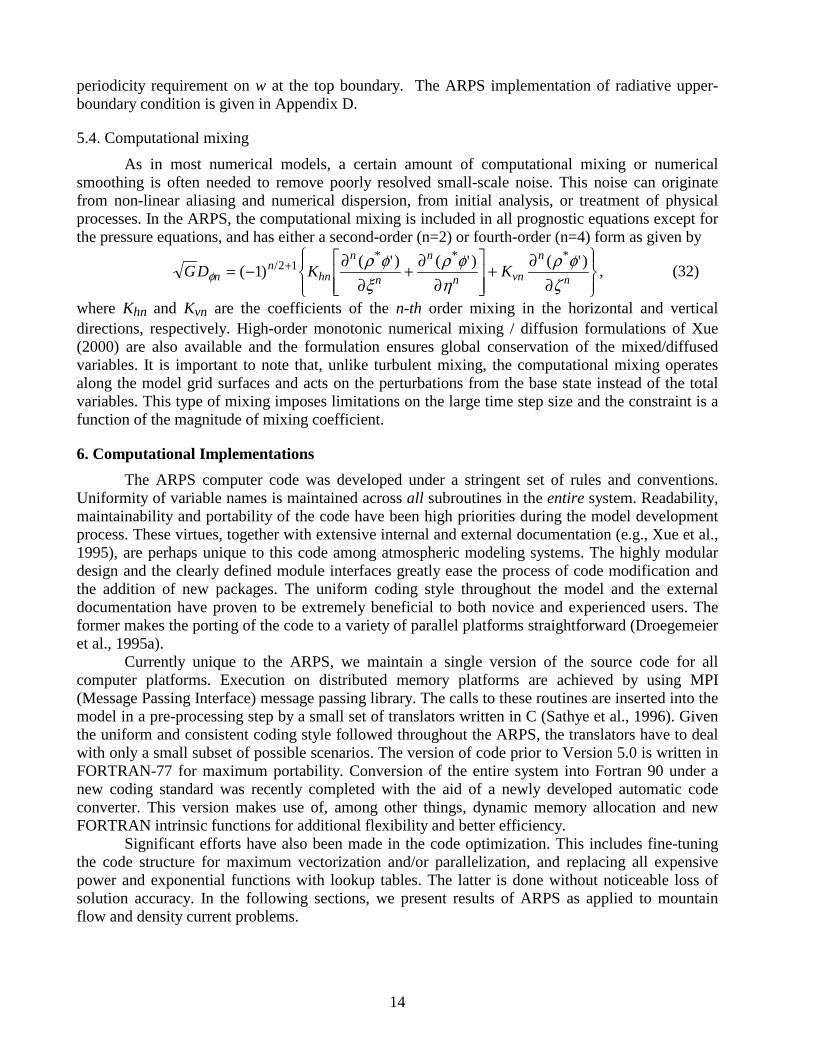
5.4. Computational mixing

As in most numerical models, a certain amount of computational mixing or numerical smoothing is often needed to remove poorly resolved small-scale noise. This noise can originate

from non-linear aliasing and numerical dispersion, from initial analysis, or treatment of physical processes. In the ARPS, the computational mixing is included in all prognostic equations except for the pressure equations, and has either a second-order (n=2) or fourth-order (n=4) form as given by

GD K Knn

hn

n

n

n

n vn

n

n

LNMM

OQPP

RS|T|

UV|W|

( )( ' ) ( ' ) ( ' )/

* * *

1 2 1 , (32)

where Khn and Kvn are the coefficients of the n-th order mixing in the horizontal and vertical

directions, respectively. High-order monotonic numerical mixing / diffusion formulations of Xue

(2000) are also available and the formulation ensures global conservation of the mixed/diffused

variables. It is important to note that, unlike turbulent mixing, the computational mixing operates

along the model grid surfaces and acts on the perturbations from the base state instead of the total variables. This type of mixing imposes limitations on the large time step size and the constraint is a

function of the magnitude of mixing coefficient.

6. Computational Implementations

The ARPS computer code was developed under a stringent set of rules and conventions. Uniformity of variable names is maintained across all subroutines in the entire system. Readability, maintainability and portability of the code have been high priorities during the model development process. These virtues, together with extensive internal and external documentation (e.g., Xue et al., 1995), are perhaps unique to this code among atmospheric modeling systems. The highly modular design and the clearly defined module interfaces greatly ease the process of code modification and

the addition of new packages. The uniform coding style throughout the model and the external documentation have proven to be extremely beneficial to both novice and experienced users. The

former makes the porting of the code to a variety of parallel platforms straightforward (Droegemeier et al., 1995a). Currently unique to the ARPS, we maintain a single version of the source code for all computer platforms. Execution on distributed memory platforms are achieved by using MPI (Message Passing Interface) message passing library. The calls to these routines are inserted into the

model in a pre-processing step by a small set of translators written in C (Sathye et al., 1996). Given

the uniform and consistent coding style followed throughout the ARPS, the translators have to deal with only a small subset of possible scenarios. The version of code prior to Version 5.0 is written in

FORTRAN-77 for maximum portability. Conversion of the entire system into Fortran 90 under a

new coding standard was recently completed with the aid of a newly developed automatic code

converter. This version makes use of, among other things, dynamic memory allocation and new

FORTRAN intrinsic functions for additional flexibility and better efficiency. Significant efforts have also been made in the code optimization. This includes fine-tuning

the code structure for maximum vectorization and/or parallelization, and replacing all expensive

power and exponential functions with lookup tables. The latter is done without noticeable loss of solution accuracy. In the following sections, we present results of ARPS as applied to mountain

flow and density current problems.

15

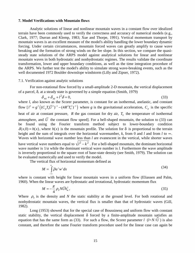
7. Model Verifications with Mountain flows

Analytic solutions of linear and nonlinear mountain waves in a constant flow over idealized

terrain have been commonly used to verify the correctness and accuracy of numerical models (e.g., Clark, 1977; Durran and Klemp, 1983; Xue and Thorpe, 1991). Vertical momentum transport by

mountain waves is an excellent measure of the model's ability handling the lower boundary dynamic

forcing. Under certain circumstances, mountain forced waves can greatly amplify to cause wave

breaking and the formation of strong winds on the lee slope. In this section, we compare the quasi-steady state solutions of the ARPS model against analytical solutions for linear and nonlinear mountain waves in both hydrostatic and nonhydrostatic regimes. The results validate the coordinate

transformation, lower and upper boundary conditions, as well as the time integration procedure of the ARPS. We further test the model's ability to simulate strong wave-breaking events, such as the

well documented 1972 Boulder downslope windstorm (Lilly and Zipser, 1972).

7.1. Verification against analytic solutions

For non-rotational flow forced by a small-amplitude 2-D mountain, the vertical displacement of a parcel, δ, at a steady state is governed by a simple equation (Smith, 1979)

δ δ δxx zz l+ + =2 0, (33) where l, also known as the Scorer parameter, is constant for an isothermal, anelastic, and constant

flow [ ( )2 2 2 1 2 2 10 0( ) (4 )pl g C T U R T− −= − where g is the gravitational acceleration, pC is the specific

heat of air at constant pressure, R the gas constant for dry air, 0T the temperature of isothermal

atmosphere, and U the constant flow speed]. For a bell-shaped mountain, the solution to (33) can

be found using the Fourier transform method subject to lower-boundary condition

δ ( , ) ( )x h x0 = , where h x( ) is the mountain profile. The solution for δ is proportional to the terrain

height and the sum of integrals over the horizontal wavenumber, k, from 0 and l and from l to ∞. Waves with horizontal wave number less than l are evanescent in the vertical, while shorter waves

have vertical wave numbers equal to l k2 2− . For a bell-shaped mountain, the dominant horizontal wave number is 1/a while the dominant vertical wave number is l. Furthermore the wave amplitude

is inversely proportional to the square root of base-state density (see Smith, 1979). The solution can

be evaluated numerically and used to verify the model.

The vertical flux of horizontal momentum defined as

' 'M u w dxρ∞

−∞

=

(34)

where is constant with height for linear mountain waves in a uniform flow (Eliassen and Palm, 1960). When the linear waves are hydrostatic and irrotational, hydrostatic momentum flux

204 mM NUh

π ρ= − , (35)

Where 0ρ is the density and N the static stability at the ground level. For both rotational and

nonhydrostatic mountain waves, the vertical flux is smaller than that of hydrostatic waves (Gill, 1982). Long (1953) showed that for the special case of Boussinesq and uniform flow with constant static stability, the vertical displacement δ forced by a finite-amplitude mountain satisfies an

equation that has the same form as (33). For such a flow, the Scorer parameter l (l= N /U ) is also

constant, and therefore the same Fourier transform procedure used for the linear case can again be

16

used to obtain the solution for δ. The main difficulty here is the enforcement of nonlinear lower boundary condition δ ( , ) ( )x z h x= .

Instead of trying to find the analytical solution for a pre-specified mountain profile that satisfies the nonlinear lower boundary condition, we follow a procedure used by Durran and Klemp

(1983) and determine a mountain profile so that the streamline given by the linear solution forced by

the original mountain follows this new profile at the lower boundary. For a bell-shaped mountain

originally 570 m high, the resultant mountain has a height of 503 m and the peak is shifted upstream

by about 400 m. In essence, the modified mountain produces nonlinear responses that are equivalent to the linear responses produced by the original taller mountain. The new mountain profile is used in

our nonlinear experiment (see Table 1) and the results will be compared with the analytic solution

obtained using the procedure outlined above. The ARPS is first verified against the 2-D solutions of linear mountain waves in both

hydrostatic and nonhydrostatic flow regimes (as in Smith, 1979). In all experiments, the earth's

rotation is neglected and an isothermal (T0 = 250 K) uniform upstream flow (U = 20 ms-1) is

specified. The experiments are impulsively started, i.e., the mountain is introduced into the flow at the initial time. The Durran and Klemp (1983) radiation lateral boundary condition option is used

for all control experiments, and the upper boundary condition uses either Rayleigh damping or the

wave permeable condition of Klemp and Durran (1983), a small amount of horizontal spatial smoothing (computational mixing) is applied only in the nonlinear run. The gravity wave modes are

integrated on the large time step. Divergence damping is not used. Three control experiments for idealized mountain waves are summarized in Table 1. For the

parameters used here we have l-1 ≈ 1 km. In experiment LH, a = 10 km » l-1, thus the flow is

essentially hydrostatic. In experiments LNH and NLNH, a = 2 km ~ l-1, the flow belongs to the

nonhydrostatic regime.

a) Linear mountain wave experiments

We present the model results at nondimensional (ND) times that are scaled by the advective

time scale U0/a. Fig. 4 shows the analytical (upper panel) and model (lower panel) solutions of u' and w' for part of computational domain at U0t/a = 100 (Note that the mountain depicted in the

figures has been amplified by a factor of 500 for illustration purpose and it is done for all linear solutions). The analytical fields were obtained by numerically integrating the integral solution using

mid-point method (Press et al., 1989). In general, the simulated waves are slightly weaker than their analytical counterparts, and the error increases with height. The maximum relative error in w' is

about 5%, while that of u' in about 14%. The phases of the waves agree very well, however. Notice

the amplitudes of the waves increase with height due to the effect of decreasing density. Vertical profiles of horizontal momentum transport by gravity wave processes are plotted in

Fig. 5 for experiment LH, together with that from the analytical solution (bold line). These profiles

have been scaled by the analytical flux for linear hydrostatic waves given in (34). It can be seen that the analytical flux is almost unity, while the simulated fluxes are about 0.97 at the surface and

approach 0.96 at later times at the level immediately below the Rayleigh damping layer (12 km). This accuracy is at least as good as those reported in the literature. For example, Durran and Klemp

(1983) reported that the flux at one vertical wavelength (z=6.4km) reached 94% of the analytical value at a ND time of 60 for their compressible model. A similar accuracy was also reported by Xue

and Thorpe (1991). The improvement in accuracy obtained here can be partly attributed to higher vertical resolution. We also performed an experiment (LHa) that is the same as LH, except that the vertical grid

is stretched from a minimum of 20 m at the surface while keeping total number of levels the same.

17

The stretching is based on a hyperbolic tangent function as described in Xue et al. (1995). The

momentum fluxes in Fig. 6 are even closer to unity (0.98) at the surface while the values at upper levels are slightly smaller, indicating that the solution accuracy is slightly sensitive to the vertical resolution. Another experiment (LHb) was conducted that used the wave-radiating top boundary

condition without Rayleigh damping. In this case, the flux profile (Fig. 7) is nearly constant, with

values being of about 96% at the surface and decreasing to 91% at the top by non-dimensional time

140. It appears that the radiation boundary condition is working well in this case. Fig. 8 shows the analytical and model simulated u' and w' fields for linear nonhydrostatic

mountain waves from experiment LNH. Evident in the solutions are the dispersive wave trains

downstream of the mountain peak, especially at upper levels, distinguishing them from the

hydrostatic solutions obtained in previous experiments. The simulated wave pattern agrees quite

well with theory, with the amplitudes being slightly smaller (as in the previous cases). Fig. 9a shows

the model simulated isentropes after θ' has been amplified by 500 times for the purpose of illustration. These isentropes approximate parcel trajectories for an adiabatic, steady-state flow. It can be seen that the lowest isentrope intercepts the terrain because of the linear boundary forcing. In

these simulations, the pressure field is found to be most sensitive to contamination at the lateral boundaries (which use an open boundary condition) in a long simulation, and it is shown in Fig. 9b

that it remains well behaved by ND time 100. The momentum flux [scaled by the hydrostatic value given by (35)] from experiment LNH

(Fig. 10) is essentially constant at later times below the Rayleigh damping layer, with a value of about 0.76. This result is very close to the theoretical prediction (Klemp and Durran, 1983) for linear nonhydrostatic mountain waves.

b) Nonlinear mountain waves

Because Long's solution requires the Boussinesq approximation, the option for this

approximation in the ARPS is turned on. It involves replacing by its constant surface value after and p are specified. We also neglect the contribution by p' to the buoyancy as well as the vertical advection of p in pressure equation. These simplifications make the system of equations analogous

to the Boussinesq equations describing an incompressible flow (the same approximations were

made in Xue et al., 1997). Finally, the atmosphere remains isothermal and 20U = so that the

Score's parameter has a value similar to that in our previous experiments. Fig. 11 shows the analytical solution of u' and w' (upper panel) for a 503 m high mountain

obtained using the procedure described in Section 7.1a. The model solutions at ND time 100 are

given in the lower panel. Since the reference state density is constant, the wave amplitude no longer increases with height; in fact, it decreases because significant wave energy is dispersed downstream. The agreement between the two solutions is very good, with the amplitudes in the numerical solution being only slightly weaker. The simulated isentropes and perturbation pressure are shown in Fig. 12. Unlike the previous

linear experiment (see Fig. 9), the isentrope at the surface closely follows the terrain, while the

waves at upper levels are weaker than those in Fig. 9 for the lack of density scaling effect. The

pressure field is again well behaved. Finally Fig. 13 shows the vertical profiles of momentum

fluxes. These fluxes have been scaled by that of hydrostatic nonlinear mountain waves, the latter given by the formulation (35) for linear waves but with hm=570 m. The profile calculated from the

analytical u' and w' from Long's equation is shown by the thick line. The simulated vertical fluxes

overshoot at the early time due to the impulsive startup but converge toward the analytical value of about 0.76. This value is very close to that in experiment LNH, indicating that both linear and

nonlinear mountain waves in the nonhydrostatic regime with al = 2 transport momentum at a rate of

18

about 76% of their hydrostatic counterparts, a result that agrees with theory (Klemp and Durran, 1983). Furthermore, the fact that the flux is nearly constant throughout the depth of domain at later times indicates that the radiation top boundary condition works well even for these finite amplitude

waves (of course the wave amplitude has been significantly reduced at upper levels due to

downstream dispersion of energy).

7.2. Simulation of 1972 Boulder windstorm

A severe windstorm developed on the lee (east) side of the Front Range of the Rocky

Mountains was well observed and documented in Lilly and Zipser (1972) and has been a subject of many subsequent studies (e.g., Klemp and Lilly, 1975; Peltier and Clark, 1979; Durran, 1986). Recently, 2D simulations of this case with a bell-shaped mountain were conducted using 11 models

(including ARPS) and the results intercompared (Doyle et al., 2000). Initialized with a upper-stream

sounding taken at Grand Junction CO over an bell-shaped mountain that resembles the Front Range, most models were able to simulate the upper-level wave breaking and intensification of downslope

winds reasonably well, although significant differences exist among the solutions. In this paper, we report the results of our simulation using a high-resolution real terrain

profile. The terrain profile is derived from a 3 second terrain database sub-sampled at 15 second

intervals. The data were bilinearly interpolated to a 1 km grid after which a 1-2-1 filter is applied

once to remove 2 grid interval terrain features. A 500km E-W cross-section through Boulder (40.027N) is taken and a 28 km deep domain is used. Radiation boundary conditions are used the

top and lateral boundaries. The latter uses the Klemp and Wilhelmson (1978) formulation with a

constant phase speed of 50 ms-1. The model is initialized with the 1200 UTC 11 January 1972

Grand Junction CO sounding (Fig. 14), which extends up to a 28 km altitude. The sounding has a

critical level (u=0) at the 23 km level, therefore waves are expected to be confined to below this

level. The sounding also contains a relatively stable layer between 5 and 7 km levels, contributing to

the intensification of downslope winds in a form of hydraulic jump flow, according to Durran and

Klemp (1986). Most previous simulation studies of this case used significantly smoothed soundings

with modified wind profile at the upper levels (e.g., Peltier and Clark, 1979; Durran and Klemp, 1983). Different from Doyle et al. (2000), care is taken here to place the lowest level of observed

sounding at the station height rather than at the sea level so as to yield a correct distance between the

mountain peak and the tropopause (and the stable layer). The grid resolution is 1 km in the

horizontal and 0.2 km in the vertical. The model flow is abruptly started and the control experiment does not include surface friction. Fig. 15 shows the potential temperature contours and cross-mountain velocity fields at 3 and

6 hours. The isentropes represent the flow trajectories reasonably well outside the regions of wave

breaking. The most significant features seen are the descent of mid-tropospherical isentropes along

the lee slope of the Front Range, accompanied by strong surface winds of over 70 and 80 ms-1 at 3

and 6 hours, respectively. The maximum surface wind reached 70 ms-1 at 2 hours 40 minutes and

remained above 70 ms-1 for the rest of the simulation. The surface wind peaked 94 ms-1

at 4 hours

47 minutes in this simulation. The strong surface winds propagate downstream with the gust front, at which the flow decelerates abruptly and transitions into a subcritical flow in the form of hydraulic

jump (Durran, 1986). Strong vertical motion is found at the front, signified by the nearly vertical isentropes. Above this strong surface flow and below tropopause, flow reversal (u<0) is seen shortly

after 3 hours, resulting in flow overturning and strong mixing. Wave overturning and breaking are

also found above the tropopause, where vertical wavelengths and amplitudes are smaller due to

higher stability. The strongest upper-level wave activities are found to be coupled with the strongest tropospheric forcing at the jump, whereas activities directly above the upper-tropospheric wave-breaking region are weak. This well mixed region acts as a critical level that, in theory, reduces the

19

vertical group velocity to zero and prevents upward transport of wave energy. The trapping of wave

energy at the lower levels tend to accelerate the low-level flow. Further upstream, waves of significant amplitude are forced by lower (relative to terrain height on the lee side) ridges near x=200 km, and these waves propagate vertically into the stratosphere forcing significant wave

breaking as well (not shown). These waves are sufficiently far upstream of the Front Range and do

not appear to have significantly affected the primary wave system by 6 hours. Due to the presence of very weak flow at about the 23 km level, nearly all wave activities are confined below 23 km (not shown). The use of radiation top boundary condition does not appear critical to the lower-level mountain flow.

Overall, the simulated wave system at the earlier time resembles the observation depicted in

Figs. 4 and 5 in Klemp and Lilly (1975). The peak surface wind speed is larger than observed, almost certainly due to the absence of surface friction. The results are also consistent with those of previous simulation studies, although most of which use an idealized ridge. Our results also agree

qualitatively well with the simulation of COAMPS reported by Dolye et al. (2000) which applied a

smoothed real terrain. The sounding used the in latter, however, assumed height above sea level instead of ground level, therefore the tropopause in their case was about 1.5 km lower than reality. A simulation repeated using their sounding results in a result closer to their solution. Finally, the

extra fine-scale terrain features included in the current experiment do not seem to significantly

impact the general behavior of the downslope flow, as is supported by experiments in which small-scale features are filtered out or when a bell shaped ridge of similar scale and height is used (not shown). This can also be understood by noting that the downslope flow is mainly fed by the flow

above the 4 km level upstream. Had the terrain upstream of the Front Range been replaced by air, the air would be too heavy (measured by the upstream Froude number) to climb the mountain range. Another experiment that included parameterized surface friction (through surface drag) resulted in a

much weaker wave system, in which the downslope winds are limited to the lee slope (not shown). This result is consistent with the finding of Richard et al. (1989).

7.3. Summary

We presented in this section a set of idealized mountain wave experiments as well a realistic

simulation of a severe downslope windstorm. For the former, analytical solutions that cover linear and nonlinear waves in both hydrostatic and nonhydrostatic flow regimes can be found. Quasi-steady state model solutions were compared against these analytical solutions and excellent agreement was found. Experiments were conducted to examine solution sensitivity to vertical grid

stretching and the top boundary condition. These experiments, as well as the simulation of a severe

downslope windstorm, demonstrated the integrity of the dynamic and numerical framework of the

model, in particular those aspects related to the coordinate transformation, the treatment of lower-boundary forcing, and the top boundary conditions.

8. Model Validation with a Nonlinear Density Current

In this section, we examine the model's ability to accurately handle highly nonlinear flow

with strong interior gradients. A benchmark problem of a simple density current is chosen. Solutions

for this problem from a number of numerical models, including those of Carpenter et al. (1990) and

Xue and Thorpe (1991), are documented in Straka et al. (1993). Particular attention is paid to

several options of advection schemes in the ARPS and their impact on the solution accuracy.

20

8.1. The Test Problem

The test consists of a 2-D density current formed from a cold blob of air descending from an

elevated level to the ground in a neutrally stratified and initially static atmosphere. As the cold air reaches the ground, it spreads along the lower boundary and develops rotors along the top of the

cold pool boundary due to Kelvin-Helmholtz instability (Fig. 16). In the spatial resolution

experiments, the eddy-mixing coefficient is kept the same, so that the solutions may converge at high resolutions. The base-state atmosphere is calm and has a constant potential temperature of 300 K. An

elliptic initial bubble is specified in terms of temperature perturbation. It is centered at x=0 km and

z= 3 km with a vertical half-axis of 2 km, a horizontal half-axis of 4 km and a minimum temperature

of -15 K (see Straka et al. 1993). Free-slip wall conditions are used on all four boundaries. The

computational domain is 6.4 km deep and 25.6 km wide. Horizontal symmetry of the problem is

exploited by centering the bubble on the left boundary. Since the amount of details that can exist in the model solution are limited by the specified

and fixed eddy mixing coefficient, it is possible to obtain a reference solution at a high resolution

beyond which no noticeable improvement can be achieved. Such a reference solution was presented

in Straka et al. (1993) using a compressible model with second-order advection at 25 m spatial resolution. We present in Fig. 16 a similar reference solution obtained using our model with fouth-order centered spatial difference, which is essentially identical to that obtained using second-order scheme (not shown). Since this solution is very close to the reference solution in Straka et al. (1993, see their Figure 2), we will use it as our benchmark.

8.2. The Model Results

We conducted a set of experiments using four options of advection schemes at 400, 200 and

100 m spatial resolutions (Table 2). The four advection options are: 1) second-order centered; 2) fourth-order centered; the flux-corrected transport (FCT) (Zalesak, 1979) with second-order (3) and

fourth-order (4) higher scheme. For the first two options, the same advection schemes were applied

to both momentum and scalars, while for the latter two, momentum was advected by the standard

fourth-order centered scheme. The details on these options can be found in Part I. FCT preserves the

monotonicity but does not require positive-definiteness, it can therefore be used to advect fields

with both signs. As a special case, a positive field will remain positive in the advective process. The

result of using FCT in the model of Xue and Thorpe (1991) is documented in Straka et al. (1993). Following Straka et al. (1993), the experiments are run at 400m, 200m and 100m resolutions. At these resolutions, the simulated density currents are, respectively, poorly resolved, reasonably

resolved and well resolved, measured in terms of the spatial resolution as compared to the

characteristic flow features. The difference in the scheme performance, as will be shown, is more

pronounced at lower resolutions. Fig. 17 shows the simulated θ' fields at 900 s, using four advection options at 400 m

resolution. The corresponding solutions using 200 m and 100 m resolutions are shown in Fig. 18

and Fig. 19, respectively. The bottom panel of each figure is the reference solution averaged to the

corresponding resolution. It is clear that undershooting in θ', as indicated by the minimum values, is

occurring near the density current head in all but the FCT solutions, with the problem being most serious at the lowest resolution. The error is generally larger with second-order scheme than with

fourth-order scheme. This undershoot, causing the cold pool to be too cold, is believed to be

responsible for the faster propagation speed of the front in all these cases. At all resolutions, the fourth-order schemes clearly outperform the second-order

counterparts, in defining the frontal location and in simulating the shape and location of the billows

21

(e.g., compare Fig. 17a and Fig. 17b, Fig. 18a and Fig. 18b). The FCT solutions are generally much

better than their non-monotonic counterparts. This is evident by comparing, e.g., Fig. 17c with Fig. 17a, and Fig. 17d with Fig. 17b. The FCT scheme not only eliminates spurious oscillations but also

resolves the fine-scale billow structures better. At 100 m resolution, the differences in the solutions

are smaller but are still readily identifiable, with the 4th-order and FCT options outperforming the

others. Among all solutions, FCT4th100 in Fig. 19d compares best with the reference solution, agreeing with our expectation. The FCT scheme is about 3 times more expensive the conventional scheme of the same order, however.

8.4. Summary

It has been documented in this section the behavior of four advection options in the ARPS, as applied to a density current for which a reference solution is obtained at much higher resolution. The monotonic FCT scheme clearly outperforms the regular centered difference schemes, especially

at relatively coarse resolutions. The fourth-order option exhibits clear improvement over the lower-order counterpart. The comparisons of these solutions with the grid-converged reference solution

obtained using ARPS as well as with the benchmark solution in Straka et al. (1993) establishes the

reliability of the model in handling highly nonlinear and transient solutions.

9. Summary and Discussion

The design philosophy, the choice of equations and their formulations, the numerical integration procedures, and the parameterizations of the subgrid-scale and PBL turbulence

processes in the ARPS have been described in this paper. The dynamical and numerical framework

of the model is verified against known solutions of mountain waves and an observed severe

downslope windstorm. It is also verified using a grid-converged solution of a nonlinear density

current. The results of the latter also clearly demonstrate the superiority of a high-order monotonic

advection scheme over conventional schemes that are commonly employed in atmospheric models. We believe the use of the generalized coordinate transform with horizontal stretching, the

treatment of terms related to terrain-following coordinate for truncation error reduction, the

formulation of conservative high-order advection terms, the implementation of monotonic advection

for scalars, the coupling of PBL with 'free atmosphere' turbulence, the coupling of soil-vegetation

model, surface layer, PBL and atmospheric radiation, as well as the computational implementation

of the system have their unique aspects compared to other regional atmospheric prediction models. The numerical framework and the computational paradigm that have been established provide a

solid foundation upon which future improvements can be rapidly implemented. It should be pointed out that only the forward time integration components of the ARPS

model system have been described here. The complete forecast system includes real time data

ingest, data analysis, retrieval and assimilation components (Brewster, 1996; Shapiro et al., 1996), the 4D adjoint based data assimilation system (Wang et al., 1995), as well as a platform-independent post-processing package. A complete description of these components is outside the scope of this

paper. More detailed description of the coupled soil-vegetation model, the treatment of surface

layer fluxes, the microphysics and cumulus parameterizations, and the radiation scheme used in the

ARPS will be presented in Part II of this paper series. Additional verification experiments and an

application of the model to the simulation of a multi-scale event containing multiple tornadic

supercell storms and an intense long-lived squall line can also be found there. The source code and

the online documentations of the ARPS are available at http://www.caps.ou.edu/ARPS.

22

Appendix A. Definition of symbols

Cp Specific heat of dry air at constant pressure (J kg-1 K-1);

sc

1/ 2( )sc RTγ= , the full acoustic wave speed (m s-1);

Cv Specific heat of dry air at constant volume (J kg-1 K-1);

Dij Deformation tensors (s-1);

f,~f Coriolis parameters. f=2Ω sin(φ) and

~f =2Ω cos(φ) (s-1) where φ is the earth latitude;

g Acceleration due to gravity (m s-2 ); Hj Turbulence heat or moisture fluxes (kg K m-2

s-1);

J1, J2, J3, J4, G Coordinate transformation Jacobians (ND);

κ,

1d pR C−

,m hK K Turbulence mixing coefficient for momentum and scalars, respectively (m2 s-1);

l Turbulent mixing length (m); L Latent heat of evaporation; m Map projection factor (ND); N Dry or moist Brunt-Väsäilä frequency, depending on local static stability (s-1);

p, p p, ' Total, base-state and perturbation pressure (Pascal); Pr Turbulent Prandtl number (ND); q Generic form of water vapor and other hydrometeor species (kg kg-1); Q Adiabatic heating rate (K s-1); qh Hail/grapaul mixing ratio (kg kg-1); qi Cloud ice mixing ratio (kg kg-1); qli Total liquid and ice water mixing ratio (kg kg-1); qr Rain water vapor mixing ratio (kg kg-1); qs Snow mixing ratio (kg kg-1); qv Water vapor mixing ratio (kg kg-1); qvs Saturation water vapor mixing ratio (kg kg-1); Rd Gas constant for dry air (J kg-1

K-1); Rv Gas constant for water vapor (J kg-1

K-1); T, T T, ' Total, base-state and perturbation temperature (K); u, v, w Cartesian velocity components in x, y and z directions (m s-1); Uc, Vc, Wc

Contravariant velocity compoments in ξ, η and ζ directions (m s-1); x, y, z Cartesian coordinates (m); Ω Angular rotation rate of the earth (s-1); γ Rd/Rv; π, Π, π' Total, base-state and perturbation Exner function. π ≡ (p/p0)

Rd/Cp and p0=105

Pascal; θe Equivalent potential temperature (K);

θ, , ' Total, base-state and perturbation potential temperature (K);

ρ∗ G (kg m-3);

ρ, , ' Total, base-state and perturbation density (kg m-3);

τij Stress tensors (kg m-1 s-2);

ξ, η, ζ Coordinates in the computational space corresponding to x, y and z (m);

23

Appendix B. The vertically implicit solution of the p and w equations

When coefficient β is not zero, Eqs. (3.4c) and (3.4d) become simultaneous equations for two unknowns, w

and p' and can not be solved independently.

After regrouping the unknown terms, we rewrite the p-equation (3.4d) as

p p g w c x y G w Fs p' ' /

2 , (B1)

where Fp includes other known terms:

FG

f G g w c x y w

c m

GJ u m J v m J u m J v m

p pt

s

s

RST

UVW

LNM

OQP

( )

( / ) ( / ) / /( ) ( )

1 2

2 2

3 4 1 2

Substituting p' τ+∆τ in (B1) into w-equation (3.4c) and regrouping again yields

w F x y g w c x y G w

g c g w c x y G w

w s

s s

LNM

OQP

( ) /

( ) ( ) / ,

*2 2

2 2 2

(B2)

where the known terms on the RHS are grouped into Fw , which is

F w f x y p F x y Div

g p F c

w wt

p

p s

LNM

OQPUVW

* *

*

'

[ '/ ( ' ) / ( )]

d i c h2

.

Eq. (B2) now has only one unknown, wτ+∆τ , and the spatial averaging and differencing are

all performed in the vertical direction. Expressing the equation in an explicit finite difference form

yields a set of linear algebraic equations for w at three adjacent vertical levels:

A w B w C w Dk k k k k k k

1 1

, (B3) where k is the index for vertical levels, and the known coefficients Ak, Bk, Ck and Dk are

A P N M Lk k k k k

( )( )1 1 ,

B N M M L L

P M M L Lk k k k k k

k k k k k

1 1 1

1 1

( )

( ) ,

C P N M Lk k k k k ( )( ) , Dk = Fw k

where

P g ck s ( ) ( )

2 22 , N x yk ( ) ( )*

2 , M gk / 2 , and L c Gk s 2 ( ) .

Equation (B3) forms a linear tridiagonal equation system and is solved using the Thomas algorithm (e.g., Richtmyer and Morton, 1967) given upper and lower boundary conditions on w. For a rigid top, w = 0. For the radiation top boundary, the inverse transform of (D4) in Appendix D is used as the condition. At the surface, w is obtained from the nonpermeable condition that requires

the flow to be parallel to the ground. Finally, the wτ+∆τ is substituted into Eq.(B1) to obtain p'τ+∆τ, thus complete one small time step integration cycle.

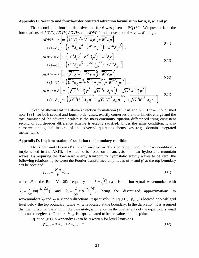
24

Appendix C. Second- and fourth-order centered advection formulation for u, v, w, and p'

The second- and fourth-order advection for θ was given in EQ.(30). We present here the

formulations of ADVU, ADVV, ADVW, and ADVP for the advection of u, v, w, θ' and p'.

ADVU = λ m U*ξδξ u

ξ+ V*ξ δηu

η+ W*ξδζu

ζ

+ (1–λ ) m U*2ξδ2ξ u

2ξ+ V*ξη δ

2ηu2η

+ W*ξζδ2ζu

2ζ ,

(C1)

ADVV = λ m U*ηδξ v

ξ+ V*η δηv

η+ W*ηδζv

ζ

+ (1–λ ) m U*ηξδ2ξ v

2ξ+ V*2η δ

2ηv2η

+ W*ηζδ2ζv

2ζ

, (C2)

ADVW = λ m U*ζδξ w

ξ+ V*ζ δηw

η+ W*ζδζw

ζ

+ (1–λ ) m U*ζξδ2ξ w

2ξ+ V*ζη δ

2ηw2η

+ W*2ζδ2ζw

2ζ

, (C3)

ADVP = λ m GξU cδξ p'

ξ+ G

ηV cδη p'

η+ G

ζW c δζ p'

ζ

+ (1–λ ) m GξU c

ξδ2ξ p'

2ξ

+ GηV c

ηδ2η p'

2η

+ GζW c

ζδ2ζ p'

2ζ

,

(C4)

It can be shown that the above advection formulation (M. Xue and S. J. Lin – unpublished note 1991) for both second and fourth-order cases, exactly conserves the total kinetic energy and the total variance of the advected scalars if the mass continuity equation differenced using consistent second or fourth-order difference scheme is exactly satisfied. Under the same condition, it also conserves the global integral of the advected quantities themselves (e.g., domain integrated momentum).

Appendix D. Implementation of radiation top boundary condition

The Klemp and Durran (1983) type wave-permeable (radiation) upper boundary condition is implemented in the ARPS. The method is based on an analysis of linear hydrostatic mountain

waves. By requiring the downward energy transport by hydrostatic gravity waves to be zero, the following relationship between the Fourier transformed amplitudes of w and p' at the top boundary can be obtained:

pN

kwnz nz

2 1

, (D1)

where N is the Brunt-Väisälä frequency and k k kx y 2 2 is the horizontal wavenumber with

sin( )kx

k xx

x

2

2

and sin( )k

y

k yy

y

2

2

being the discretized approximations to

wavenumbers kx and ky in x and y directions, respectively. In Eq.(D1), pnz2 is located one-half grid

level below the top boundary, while wnz-1 is located at the boundary. In the derivation, it is assumed

that the horizontal variation in the base-state, and hence, in the coefficients of the equation, is small and can be neglected. Further, pnz2 is approximated to be the value at the w point. Equation (B1) in Appendix B can be rewritten for level k=nz-2 as

p a w b w cnz nz nz'

2 1 2 (D2)

25

where ag c x y

Gs

FHG

IKJ

2

2

, bg c x y

Gs

FHG

IKJ

2

2

and c F pp nz

' 2 . Note that we

have dropped the superscript for convenience. Performing a double Fourier transform on

(D2), and assuming that the coefficients are slowly varying functions of x and y, Eq.(D2) becomes

p a w b w cnz nz nz

2 1 2 . (D3)

Eliminating pnz2 from (D1) and (D3) yields

aN

kw b w cnz nz

FHG

IKJ

1 2 0 (D4)

which, after being transformed back into the physical space, serves as the top boundary condition required by (B3). The pressure at the top boundary is then obtained from Eq.(D2).

Acknowledgements

The Center for Analysis and Prediction of Storms was supported by the National Science Foundation and Federal Aviation Administration through combined Grant and Cooperative Agreement ATM92-20009. A special acknowledgment is in order for our colleagues who contributed in various ways to the development and testing of the ARPS. We would like to thank H. Jin, D. Weber, Y. Liu, X. Song, D.-H. Wang, A. Sathye, D. Jahn, L. Zhao, G. Bassett, R. Carpenter, D.H. Wang, D. Hou, J. Zong, S. Weygandt, J. Levit, S. Lazarus, J. Zhang, Y. Richardson, Y. Tang, M. Zou, and S.-K. Park. Special thanks go to Dr. Alan Shapiro, who led a local users group in the early days that tested various versions of the model, to Dr. Keith Brewster, who is the author of ADAS, and to Dr. Fred Carr, who is instrumental in the development of the data analysis system. We have benefited greatly from collaborations and exchanges with numerous scientists, including Drs. W. Skamarock, A. Crook, J. Dudhia, G. Tripoli, W.-K. Tao, J. Straka, L. Wicker, J.S. Kain, C. Mattocks. Keith Brewster and Dan Weber are thanked for reviewing the manuscript.

References Arakawa, A., and V. R. Lamb, 1977: Computational design of the basic dynamical processes of the

UCLA general circulation model. In: J. Chang (Editor), Methods in Computational Physics. Academic Press, 174-264.

Batchelor, G. K., 1967: An Introduction to Fluid Dynamics. Cambridge University Press, 615 pp. Brewster, K., 1996: Application of a Bratseth analysis scheme including Doppler radar data.

Preprints, 15th Conference on Weather Analysis and Forecasting. Amer. Meteor. Soc., Norfolk, VA, 92-95.

Carpenter, R. L., K. K. Droegemeier, P. R. Woodward, and C. E. Hane, 1990: Application of the

piecewise parabolic method ( PPM) to meteorological modeling. Mon. Wea. Rev., 118, 586-612.

Caughey, S. J., J. C. Wyngaard, and J. C. Kaimal, 1979: Turbulence in the evolving stable boundary

layer. J. Atmos. Sci., 36, 1041-1052. Chen, C., 1991: A nested grid, nonhydrostatic, elastic model using a terrain-following coordinate

transformation: The radiative-nesting boundary conditions. Mon. Wea. Rev., 119, 2852-2869.

Chou, M.-D., 1990: Paramemterization for the absorbtion of solar radiation by O2 and CO2 with

application to climate studies. J. Climate, 3, 209-217. Chou, M.-D., 1992: A solar radiation model for climate studies. J. Atmos. Sci., 49, 762-772.

26

Chou, M.-D., and M. J. Suarez, 1994: An efficient thermal infrared radiation parameterization for

use in general circulation models, NASA Tech. Memo. 104606, 85pp. [Available from NASA Center for Aerospace Information, 800 Elkridge Landing Road, Linthicum Heights, MD 21090-2934.].

Clark, T. L., 1977: A small-scale dynamic model using a terrain-following coordinate

transformation. J. Comput. Phys., 24, 186-215. Crum, T. D., and R. L. Albert, 1993: The WSR-88D and the WSR-88D operational support facility.

Bull. Amer. Meteor. Soc., 74, 1669-1687. Cullen, M. J. P., 1990: A test of a semi-implicit integration technique for a fully compressible non-

hydrostatic model. Quart. J. Roy. Meteor. Soc., 116, 1253-1258. Davies, H. C., 1983: Limitations of some common lateral boundary schemes used in regional NWP

models. Mon. Wea. Rev., 111, 1002-1012. Deardorff, J. W., 1972: Numerical investigation of neutral and unstable planetary boundary layers.

J. Atmos. Sci., 29, 91-115. Deardorff, J. W., 1980: Stratocumulus-capped mixed layers derived from a three-dimensional

model. Bound. Layer Meteor., 18, 495-527. Doyle, J. D., D. R. Durran, B. A. Colle, C. Chen, M. Georgelin, V. Grubisic, W. R. Hsu, C. Y.

Huang, D. Landau, Y. L. Lin, G. S. Poulos, W.Y.Sun, D. B. Weber, M. G. Wurtele, and M. Xue, 2000: An intercomparison of model-predicted wave breaking for the 11 January 1972 Boulder windstorm. Mon. Wea. Rev., 901-914.

Droegemeier, K. K., 1990: Toward a science of storm-scale prediction. Preprint, 16th conf. on

Severe Local Storms. Amer. Meteor. Soc., Kananaskis Park, Alberta, Canada, 256-262. Droegemeier, K. K., M. Xue, K. Johnson, M. O'Keefe, A. Sawdey, G. Sabot, S. Wholey, N. T. Lin,

and K. Mills, 1995a: Weather prediction: A scalable storm-scale model. In: G. Sabot (Editor), High Performance Computing. Addison-Wesley, Reading, Massachusetts, 45-92.

Droegemeier, K. K., M. Xue, K. Johnson, M. O'Keefe, A. Sawdey, G. Sabot, S. Wholey, and K. Mills, 1995b: Design and Implementation of a Scalable-Parallel Stormscale Numerical Weather Prediction Model. In: G.W. Sabot (Editor), High Performance Computing. Addison-Wesley, Reading, Massachusetts, 45-92.

Dudhia, J., 1993: A nonhydrostatic version of the Penn State-NCAR mesoscale model: Validation

tests and simulation of an Atlantic cyclone and cold front. Mon. Wea. Rev., 121, 1493-1513. Durran, D. R., 1986: Another look at downslope windstorms. Part I: The development of analogs to

supercritical flow in an infinitely deep continuously stratified field. J. Atmos. Sci., 43, 2527-2543.

Durran, D. R., 1989: Improving the anelastic approximation. J. Atmos. Sci., 46, 1453-1461. Durran, D. R., and J. B. Klemp, 1982: On the effects of moisture on the Brunt-Väisälä frequency. J.

Atmos. Sci., 39, 2152-2158. Durran, D. R., and J. B. Klemp, 1983: A compressible model for the simulation of moist mountain

waves. Mon. Wea. Rev., 111, 2341-2361. Dutton, J. A., 1986: The Ceaseless Wind, An Introduction to the Theory of Atmospheric Motion.

McGraw-Hill, New York, 617 pp. Eliassen, A., and E. Palm, 1960: On the transfer of energy in stationary mountain waves. Geophys.

Norv., 22, 1-23. Fiedler, B., Z. Huo, and P. Zhang, 1998: Dynamic grid adaption for atmospheric boundary layers.

Preprint, 12th Conf. Numerical Wea. Prediction. Amer. Meteor. Soc., Phoenix, 64-67. Germano, M., U. Piomelli, P. Moin, and W. H. Cabot, 1991: A dynamic subgrid-scale eddy

viscosity model. Phys. Fluids, A3, 1760-1765. Gill, A. E., 1982: Atmosphere-Ocean Dynamics. Academic Press, New York, 662 pp.

27

Golding, B. W., 1990: The Meteorological Office mesoscale model. Meteor. Mag., 119, 81-96. Haltiner, G. J., and R. T. Williams, 1980: Numerical Prediction and Dynamic Meteorology. John

Wiley and Sons, 477 pp. Hodur, R. M., 1997: The U.S. Navy's coupled ocean/atmosphere mesoscale prediction system

(COAMPS). Mon. Wea. Rev., 125, 1414-1430. Janjic, Z. I., 1977: Pressure gradient force and advection scheme used for forecasting with steep and

small scale topography. Contrib. Atmos. Sci., 50, 186-199. Johnson, K. W., G. A. J. Bauer, Riccardi, K. K. Droegemeier, and M. Xue, 1994: Distributed

processing of a regional prediction model. Mon. Wea. Rev., 122, 2558-2572. Kain, J. S., and J. M. Fritsch, 1990: A one-dimensional entraining/detraining plume model and its

application in convective parameterization. J. Atmos. Sci., 47, 2784-2802. Kain, J. S., and J. M. Fritsch, 1993: Convective parameterization for mesoscale models: The Kain-

Fritsch scheme, The Representation of Cumulus Convection in Numerical Models, Meteor. Monogr. Amer. Meteor. Soc., 165-170.

Kapitza, H., 1991: Numerical experiments with the adjoint of a non-hydrostatic mesoscale model. Mon. Wea. Rev., 119, 2993-3011.

Kessler, E., 1969: On the Distribution and Continuity of Water Substance in Atmospheric

Circulations, 84 pp. Klemp, J. B., 1987: Dynamics of tornadic thunderstorms. Annul Rev. Fluid. Mech., 19, 369-402. Klemp, J. B., and D. R. Durran, 1983: An upper boundary condition permitting internal gravity

wave radiation in numerical mesoscale models. Mon. Wea. Rev., 111, 430-444. Klemp, J. B., and D. K. Lilly, 1975: The dynamics of wave-induced downslope winds. J. Atmos.

Sci., 32, 320-339. Klemp, J. B., and R. B. Wilhelmson, 1978: The simulation of three-dimensional convective storm

dynamics. J. Atmos. Sci., 35, 1070-1096. Kuo, H. L., 1965: On the formation and intensification of tropic cyclones through latent heat release

by cumulus convection. J. Atmos. Sci., 22, 40-63. Kuo, H. L., 1974: Further studies of the parameterization of the influence of cumulus convection on

large-scale flow. J. Atmos. Sci., 31, 1232-1240. Lafore, J. P., J. Stein, N. Asencio, P. Bougeault, V. Ducrocq, J. Duron, C. Fisher, P. Péreil, P.

Mascart, V. Masson, J. P. Pinty, J. L. Redelsperger, E. Richard, J. Vilà-Guerau de Arellano, 1998: The meso-NH atmosperhic simulation system. Part I: Adiabatic formulation and

control simulation. Ann. Geophysicae, 16, 90-109. Lilly, D. K., 1962: On numerical simulation of buoyant convection. Tellus, 14, 148-172. Lilly, D. K., 1979: The dynamical structure and evolution of thunderstorms and squall lines. Annu.

Rev. Earth Planet. Sci., 7, 117-171. Lilly, D. K., 1990: Numerical prediction of thunderstorms - Has its time come? Quart. J. Roy.

Meteor. Soc., 116, 779-798. Lilly, D. K., and E. J. Zipser, 1972: The Front Range windstorm of 11 January 1972. Weatherwise,

25, 56-53. Lin, Y.-L., R. D. Farley, and H. D. Orville, 1983: Bulk parameterization of the snow field in a cloud

model. J. Climate Appl. Meteor., 22, 1065-1092. Liou, Y. C., T. Cal-Chen, and D. K. Lilly, 1991: Retrievals of wind, temperature and pressure from

single-Doppler radar and a numerical model. Preprint, 25th Int. Conf. on Radar Meteor. Amer. Meteor. Soc., Paris, France, 151-154.

Long, R. R., 1953: Some aspects of the flow of stratified fluids. I. A theoretical investigation. Tellus, 5, 42-58.

28

Mesinger, F., and Z. I. Janjic, 1985: Problems and numerical methods of incorporation of mountains in atmospheric models, Lectures in Applied Mathematics. Amer. Math. Soc., 81-119.

Miller, M. J., and R. P. Pearce, 1974: A three-dimensional primitive equation model of cumulonimbus convection. Quart. J. Roy. Meteor. Soc., 100, 133- 154.

Moeng, C.-H., 1984: A large-eddy-simulation model for the study of planetary boundary layer turbulence. J. Atmos. Sci., 41, 2052-2062.

Noilhan, J., and S. Planton, 1989: A simple parameterization of land surface processes for meteorological models. Mon. Wea. Rev., 117, 536-549.

Orlanski, I., 1976: A simple boundary condition for unbounded hyperbolic flows. J. Comput. Phys., 21, 251-269.

Orville, H. D., 1968: Ambient wind effects on the initiation and development of cumulus clouds

over mountains. J. Atmos. Sci., 2, 385-403. Peltier, W. R., and T. L. Clark, 1979: The evolution and stability of finite-amplitude mountain

waves. Part II. Surface wave drag and severe downslope windstorms. J. Atmos. Sci., 36, 1498-1529.

Pielke, R. A., and C. L. Martin, 1981: The derivation of a terrain-following coordinate system for use in a hydrostatic model. J. Atmos. Sci., 38, 1707-1713.

Pleim, J. E., and A. Xiu, 1995: Development and testing of a surface flux and planetary boundary

layer model for application in mesoscale models. J. Appl. Meteor., 34, 16-32. Press, W. H., B. P. Flannery, S. A. Teukolsky, and W. T. Vetterling, 1989: Numerical Recipes.

Cambride Univer. Press, 702 pp. Qiu, C.-J., and Q. Xu., 1992: A simple adjoint method of wind analysis for single-Doppler data. J.

Atmos. Oceanic Technol., 9, 588-598. Richard, E., P. Mascart, and E. C. Nickerson, 1989: The role of surface friction in downslope

windstorms. J. Appl. Meteor., 28, 241-251. Richtmyer, R. D., and K. W. Morton, 1967: Difference Methods for Initiai Value Problems. J.

Wiley and Sons, 405 pp. Sathye, A., G. Bassett, K. Droegemeier, M. Xue, and K. Brewster, 1996: Experiences using high

performance computing for operational storm scale weather prediction, Concurrency: Practice and Experience, special issue on Commercial and industrial Applications on High

Performance Computing. John Wiley & Sons, Ltd., 731-740. Schlesinger, R. E., 1975: A three-dimensional numerical model of an isolated deep convective

cloud: Preliminary results. J. Atmos. Sci., 32, 934-957. Schultz, P., 1995: An explicit cloud physics parameterization for operational numerical weather

prediction. Mon. Wea. Rev., 123, 3331-3343. Shapiro, A., S. Ellis, and J. Shaw, 1995: Single-Doppler radar retrievals with Phoenix II data: Clear

air and microburst wind retrievals in the planetary boundary layer. J. Atmos. Sci., 52, 1265-1287.

Shapiro, A., L. Zhao, S. Weygandt, K. Brewster, S. Lazarus, and K. K. Droegemeier, 1996: Initial forecast fields from single-Doppler wind retrieval, thermodynamic retrieval and ADAS. Preprints, 11th Conference on Numerical Weather Prediction. Amer. Meteor. Soc., Norfolk, VA, 119-121.

Sharman, R. D., T. L. Keller, and M. G. Wurtele, 1988: Incompressible and anelastic flow

simulations on numerically generated grids. Mon. Wea. Rev., 116, 1124-1136. Shyy, W., and T. C. Vu, 1991: On the adoption of velocity variable and grid system for fluid flow

computation in curvilinear coordinates. J. Comput. Phys., 92, 82-105. Skamarock, W., and J. B. Klemp, 1994: Efficiency and accuracy of the Klemp-Wilhelmson time-

splitting technique. Mon. Wea. Rev., 122, 2623-2630.

29

Skamarock, W. C., and J. B. Klemp, 1992: The stability of time-split numerical methods for the

hydrostatic and nonhydrostatic elastic equations. Mon. Wea. Rev., 120, 2109-2127. Skamarock, W. C., and J. B. Klemp, 1993: Adaptive grid refinement for two-dimensional and three-

dimensional nonhydrostatic atmospheric flow. Mon. Wea. Rev., 121, 788-804. Smagorinsky, J., 1963: General circulation experiments with the primitive equations. Part. I. The

basic experiment. J. Meteor., 14, 184-185. Smith, R. B., 1979: The influence of mountains on the atmosphere. Adv. Geophys., 21, 87-230. Steiner, J. T., 1973: A three-dimensional model of cumulus cloud development. J. Atmos. Sci., 30,

414-435. Straka, J. M., R. B. Wilhelmson, L. J. Wicker, J. R. Anderson, and K. K. Droegemeier, 1993:

Numerical solutions of a non-linear density current: A benchmark solution and comparisons. Int. J. Numer. Methods, 17, 1-22.

Sun, J., and N. A. Crook, 1994: Wind and thermodynamic retrieval from single-Doppler radar measurements of a gust front observed during Phoenix II. Mon. Wea. Rev., 122, 1075-1091.

Sun, J., D. W. Flicker, and D. K. Lilly, 1991: Recovery of three-dimensional wind and temperature

fields from simulated single-Doppler radar data. J. Atmos. Sci., 48, 876-890. Sun, W.-Y., and C.-Z. Chang, 1986: Diffusion model for a convective layer. Part I: Numerical

simulation of convective boundary layer. J. Climate Appl. Meteor., 25, 1445-1453. Tanguay, M., A. Robert, and R. Laprise, 1990: A semi-implicit semi-Lagrangian fully compressible

regional forecast model. Mon. Wea. Rev., 118, 1970-1980. Tao, W.-K., S. Lang, J. Simpson, C.-H. Sui, B. Ferrier, and M.-D. Chou, 1996: Mechanism of

cloud-radiation interaction in the tropics and mid-latitude. J. Atmos. Sci., 53, 2624-2651. Tapp, M. C., and P. W. White, 1976: A non-hydrostatic mesoscale model. Quart. J. Roy. Meteor.

Soc., 102, 277-296. Thompson, J. F., Z. U. A. Warsi, and C. W. Mastin, 1985: Numerical Grid Generation:

Foundations and Applications. North-Holland, 483 pp. Tripoli, G. J., 1992: A nonhydrostatic mesoscale model designed to simulate scale interaction. Mon.

Wea. Rev., 120, 1342-1359. Tripoli, G. J., and W. R. Cotton, 1981: The use of ice-liquid water potential temperature as a

thermodynamic variable in deep atmospheric models. Mon. Wea. Rev., 109, 1094-1102. Tripoli, G. J., and W. R. Cotton, 1982: The Colorado State University three-dimensional cloud-

mesoscale model-1982. Part I: General theoretical framework and sensitivity experiments. J. Rech. Atmos., 16, 273-304.

Wang, Z., K. K. Droegemeier, M. Xue, and S. K. Park, 1995: Sensitivity analysis of a 3-D compressible storm-scale model to input parameters. Proc., Int. Symp. on Assimilations of Observations in Meteor. and Oceanography. World Meteorological Organization, Tokyo, Japan, 437-442.

Wilhelmson, R. B., and C.-S. Chen, 1982: A simulation of the development of successive cells

along a cold outflow boundary. J. Atmos. Sci., 39, 1466-1483. Wong, V. C., 1992: A proposed statistical-dynamical closure method for the linear or nonlinear

subgrid-scale stresses. Phys. Fluids, A4, 1080-1082. Wong, V. C., 1994: A 2-way interacted boundary layer parameterization and the simulation of a

supercell storm. Proceedings, 6th Conference on Mesoscale Processes. Amer. Meteor. Soc., Portland, Oregon, 300-303.

Wong, V. C., and D. K. Lilly, 1994: A comparison of two dynamic subgrid closure methods for turbulent thermal convection. Phys. Fluids, 6, 1016-1023.

Wyngaard, J. C., and R. A. Brost, 1984: Top-down and bottom-up diffusion of a scalar in the

convective boundary layer. J. Atmos. Sci., 41, 102-112.

30

Xue, M., 2000: High-order monotonic numerical diffusion and smoothing. Mon. Wea. Rev., In press.

Xue, M., K. K. Droegemeier, V. Wong, A. Shapiro, and K. Brewster, 1995: ARPS Version 4.0

User's Guide. Center for Analysis and Prediction of Storms, [Available from CAPS, Univ. of Oklahoma, 100 E. Boyd St., Norman OK 73019], 380 pp.

Xue, M., K. K. Droegemeier, V. Wong, A. Shapiro, K. Brewster, F. Carr, D. Weber, Y. Liu, and D.-H. Wang, 2000: The Advanced Regional Prediction System (ARPS) - A multiscale nonhydrostatic atmospheric simulation and prediction tool. Part II: Model physics and applications. Submitted to Meteor. Atmos. Physics.

Xue, M., and A. J. Thorpe, 1991: A mesoscale numerical model using the nonhydrostatic pressure-based sigma-coordinate equations: Model experiments with dry mountain flows. Mon. Wea. Rev., 119, 1168-1185.

Xue, M., Q. Xu, and K. K. Droegemeier, 1997: A theoretical and numerical study of density

currents in non-constant shear flows. J. Atmos. Sci, 54, 1998-2019. Zalesak, S. T., 1979: Fully multidimensional flux-corrected transport algorithms for fluids. J.

Comput. Phys., 31, 335-362.

31

Table 1. List of mountain wave experiments

Experiment Parameters

Linear

hydrostatic (LH)

Linear nonhydrostatic

(LNH)

Nonlinear nonhydrostatic

(NLNH)

Boulder Windstorm

(WSTORM) hm (m) 1 1 503 Real terrain

a (m) 10000 2000 2000 N.A. ∆x (m) 2000 400 400 1000

∆z (m) 125 125 125 200

L (domain width, km) 576 460 460 512

H (domain depth, km) 24 24 24 28

∆t (s) 20 10 5 2.5

∆τ (s) 5 1 1 2.5

Rayleigh damping coefficient (1/s)

0.0015 0.0015 N.A. N.A.

Height damper starts (km) 12 12 N.A. N.A. 4th-order horizontal

mixing coefficient (1/s) 0 0 3×10-5 8×10−4

Table 2. List of density current experiments

Spatial resolution (m) Advection scheme

400 200 100

2nd-order-centered 2nd400 2nd200 2nd100

4th-order-centered 4th400 4th200 4th100

2nd-order FCT FCT2nd400 FCT2nd200 FCT2nd100

4th-order FCT FCT4th400 FCT4th200 FCT4th100

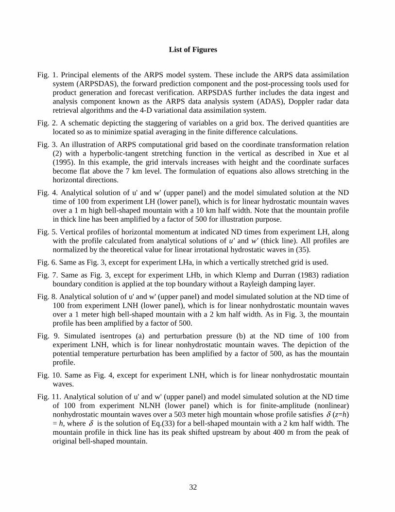
32

List of Figures

Fig. 1. Principal elements of the ARPS model system. These include the ARPS data assimilation system (ARPSDAS), the forward prediction component and the post-processing tools used for product generation and forecast verification. ARPSDAS further includes the data ingest and analysis component known as the ARPS data analysis system (ADAS), Doppler radar data retrieval algorithms and the 4-D variational data assimilation system.

Fig. 2. A schematic depicting the staggering of variables on a grid box. The derived quantities are located so as to minimize spatial averaging in the finite difference calculations.

Fig. 3. An illustration of ARPS computational grid based on the coordinate transformation relation (2) with a hyperbolic-tangent stretching function in the vertical as described in Xue et al (1995). In this example, the grid intervals increases with height and the coordinate surfaces become flat above the 7 km level. The formulation of equations also allows stretching in the horizontal directions.

Fig. 4. Analytical solution of u' and w' (upper panel) and the model simulated solution at the ND time of 100 from experiment LH (lower panel), which is for linear hydrostatic mountain waves over a 1 m high bell-shaped mountain with a 10 km half width. Note that the mountain profile in thick line has been amplified by a factor of 500 for illustration purpose.

Fig. 5. Vertical profiles of horizontal momentum at indicated ND times from experiment LH, along with the profile calculated from analytical solutions of u' and w' (thick line). All profiles are normalized by the theoretical value for linear irrotational hydrostatic waves in (35).

Fig. 6. Same as Fig. 3, except for experiment LHa, in which a vertically stretched grid is used.

Fig. 7. Same as Fig. 3, except for experiment LHb, in which Klemp and Durran (1983) radiation boundary condition is applied at the top boundary without a Rayleigh damping layer.

Fig. 8. Analytical solution of u' and w' (upper panel) and model simulated solution at the ND time of 100 from experiment LNH (lower panel), which is for linear nonhydrostatic mountain waves over a 1 meter high bell-shaped mountain with a 2 km half width. As in Fig. 3, the mountain profile has been amplified by a factor of 500.

Fig. 9. Simulated isentropes (a) and perturbation pressure (b) at the ND time of 100 from experiment LNH, which is for linear nonhydrostatic mountain waves. The depiction of the potential temperature perturbation has been amplified by a factor of 500, as has the mountain profile.

Fig. 10. Same as Fig. 4, except for experiment LNH, which is for linear nonhydrostatic mountain waves.

Fig. 11. Analytical solution of u' and w' (upper panel) and model simulated solution at the ND time of 100 from experiment NLNH (lower panel) which is for finite-amplitude (nonlinear) nonhydrostatic mountain waves over a 503 meter high mountain whose profile satisfies δ (z=h) = h, where δ is the solution of Eq.(33) for a bell-shaped mountain with a 2 km half width. The

mountain profile in thick line has its peak shifted upstream by about 400 m from the peak of original bell-shaped mountain.

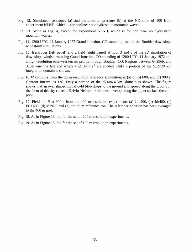
33

Fig. 12. Simulated isentropes (a) and perturbation pressure (b) at the ND time of 100 from experiment NLNH, which is for nonlinear nonhydrostatic mountain waves.

Fig. 13. Same as Fig. 4, except for experiment NLNH, which is for nonlinear nonhydrostatic mountain waves.

Fig. 14. 1200 UTC, 11 Jaunary 1972 Grand Junction, CO sounding used in the Boulder downslope windstorm simulations.

Fig. 15. Isentropes (left panel) and u field (right panel) at hour 3 and 6 of the 2D simulation of downslope windstorm using Grand Junction, CO sounding of 1200 UTC, 11 January 1972 and

a high-resolution east-west terrain profile through Boulder, CO. Regions between θ=296K and

316K one the left and where u 30 ms-1 are shaded. Only a portion of the 512×28 km

integration domain is shown.

Fig. 16. θ' contours from the 25 m resolution reference simulation, at (a) 0, (b) 600, and (c) 900 s. Contour interval is 1°C. Only a portion of the 25.6×6.4 km2

domain is shown. The figure shows that an oval shaped initial cold blob drops to the ground and spread along the ground in the form of density current. Kelvin-Helmholtz billows develop along the upper surface the cold pool.

Fig. 17. Fields of θ' at 900 s from the 400 m resolution experiments (a) 2nd400, (b) 4th400, (c) FCT400, (d) MP400 and (e) the 25 m reference run. The reference solution has been averaged to the 400 m grid.

Fig. 18. As in Figure 13, but for the set of 200 m resolution experiments.

Fig. 19. As in Figure 13, but for the set of 100 m resolution experiments.

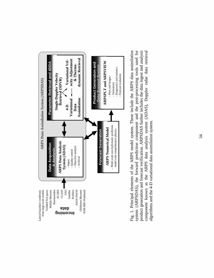
34

AR

PS

Dat

a A

naly

sis

Syst

em (

AD

AS)

AR

PS

Num

eric

al M

odel

– M

ulti-

scal

e no

n-hy

dros

tatic

pre

dict

ion

m

odel

with

com

preh

ensi

ve p

hysi

cs

– P

lots

and

imag

es

– A

nim

atio

ns

– D

iagn

ostic

s an

d st

atis

tics

– Fo

reca

st e

valu

atio

n

– In

gest

– Q

ualit

y co

ntro

l –

Obj

ectiv

e an

alys

is

– A

rchi

val

Sing

le-D

oppl

er V

eloc

ity

Ret

riev

al (

SDV

R)

4-D

V

aria

tion

al

Dat

a A

ssim

ilati

on

Var

iati

onal

Vel

-oc

ity

Adj

ustm

ent

& T

herm

o-dy

nam

ic R

etri

eval

AR

PS

Dat

a A

ssim

ilati

on S

yste

m (

AR

PSD

AS)

AR

PSP

LT

and

AR

PSV

IEW

Incoming data

Okl

ahom

a M

eson

etW

SR-8

8D W

ideb

and

AS

OS

/AW

OS

SA

O

AC

AR

S

CL

AS

S

Mob

ile M

eson

et

Pro

file

rs

Raw

inso

ndes

Sat

ellit

e

Lat

eral

bou

ndar

y co

nditi

ons

from

larg

e-sc

ale

mod

els

Gri

dded

fir

st g

uess

Dat

a A

cqu

isit

ion

&

An

alys

isD

ata

Acq

uis

itio

n

& A

nal

ysis

Fo

reca

st G

ener

atio

nF

ore

cast

Gen

erat

ion

Par

amet

er R

etri

eval

an

d 4

DD

AP

aram

eter

Ret

riev

al a

nd

4D

DA

Pro

du

ct G

ener

atio

n a

nd

D

ata

Su

pp

ort

Sys

tem

Pro

du

ct G

ener

atio

n a

nd

D

ata

Su

pp

ort

Sys

tem

Fig.

1.

Prin

cipa

l el

emen

ts o

f th

e A

RP

S m

odel

sys

tem

. T

hese

inc

lude

the

AR

PS

dat

a as

sim

ilatio

n sy

stem

(A

RP

SD

AS

),

the

forw

ard

pred

ictio

n co

mpo

nent

an

d th

e po

st-p

roce

ssin

g to

ols

used

fo

r pr

oduc

t ge

nera

tion

and

fore

cast

ver

ific

atio

n. A

RP

SD

AS

fur

ther

incl

udes

the

data

inge

st a

nd a

naly

sis

com

pone

nt

know

n as

th

e A

RP

S

data

an

alys

is

syst

em

(AD

AS

),

Dop

pler

ra

dar

data

re

trie

val

algo

rith

ms

and

the

4-D

var

iatio

nal d

ata

assi

mila

tion

syst

em.

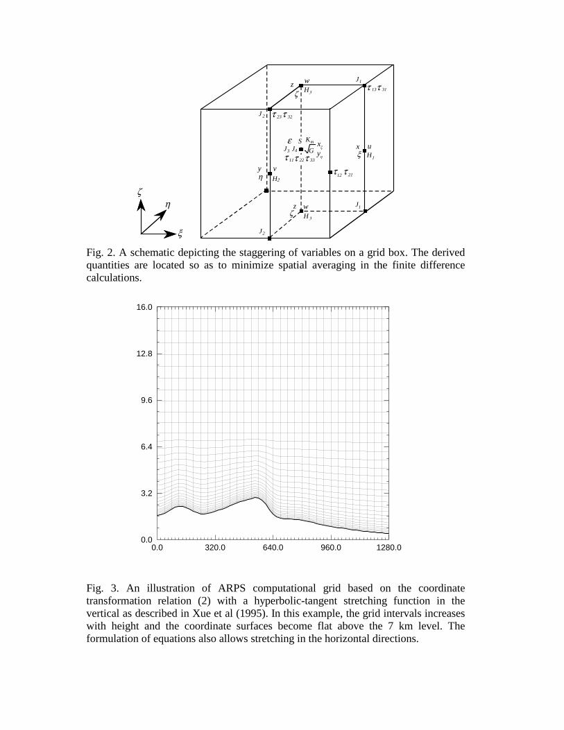
u

v

J3

J1wz

x

y

wz J1

ξ

ηζ

13τ 31τ

ε

3H

2H

H

mK

3H

12τ 21τ

23 32ττ

2J

2J

133τ22τ11τ

η

ζ

ξ

ζ

J4

S

Gxξ

yη

Fig. 2. A schematic depicting the staggering of variables on a grid box. The derived quantities are located so as to minimize spatial averaging in the finite difference calculations.

0.0 320.0 640.0 960.0 1280.00.0

3.2

6.4

9.6

12.8

16.0

Fig. 3. An illustration of ARPS computational grid based on the coordinate transformation relation (2) with a hyperbolic-tangent stretching function in the vertical as described in Xue et al (1995). In this example, the grid intervals increases with height and the coordinate surfaces become flat above the 7 km level. The formulation of equations also allows stretching in the horizontal directions.

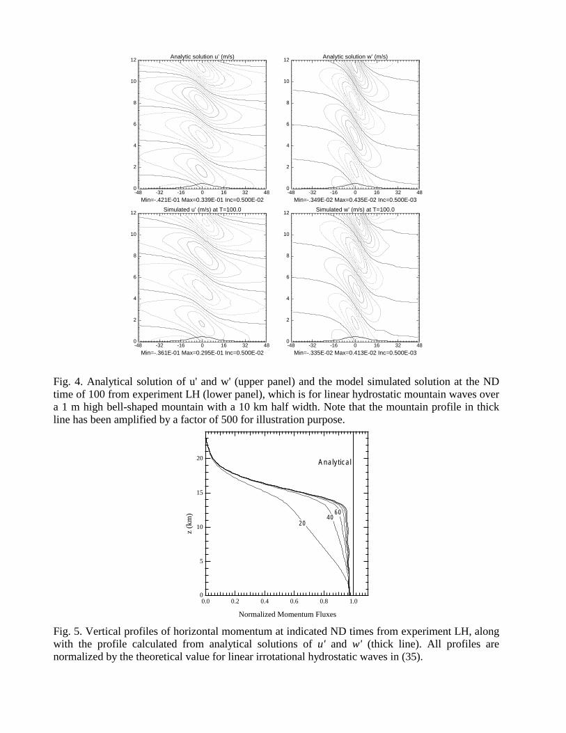
-48 -32 -16 0 16 32 480

2

4

6

8

10

12

Min=-.421E-01 Max=0.339E-01 Inc=0.500E-02

Analytic solution u’ (m/s)

-48 -32 -16 0 16 32 480

2

4

6

8

10

12

Min=-.349E-02 Max=0.435E-02 Inc=0.500E-03

Analytic solution w’ (m/s)

-48 -32 -16 0 16 32 480

2

4

6

8

10

12

Min=-.361E-01 Max=0.295E-01 Inc=0.500E-02

Simulated u’ (m/s) at T=100.0

-48 -32 -16 0 16 32 480

2

4

6

8

10

12

Min=-.335E-02 Max=0.413E-02 Inc=0.500E-03

Simulated w’ (m/s) at T=100.0

Fig. 4. Analytical solution of u' and w' (upper panel) and the model simulated solution at the ND time of 100 from experiment LH (lower panel), which is for linear hydrostatic mountain waves over a 1 m high bell-shaped mountain with a 10 km half width. Note that the mountain profile in thick line has been amplified by a factor of 500 for illustration purpose.

1.00.80.60.40.20.0

20

15

10

5

0

z (k

m)

Normalized Momentum Fluxes

2040

60

Analytical

Fig. 5. Vertical profiles of horizontal momentum at indicated ND times from experiment LH, along with the profile calculated from analytical solutions of u' and w' (thick line). All profiles are normalized by the theoretical value for linear irrotational hydrostatic waves in (35).

1.00.80.60.40.20.0

20

15

10

5

0

z (k

m)

Normalized Momentum Fluxes

2060

40

Analytical

Fig. 6. Same as Fig. 4, except for experiment LHa, in which a vertically stretched grid is used.

1.00.80.60.40.20.0

20

15

10

5

0

z (k

m)

Normalized Momentum Fluxes

20

4060

80 140

Ana

lytic

al

Fig. 7. Same as Fig. 4, except for experiment LHb, in which Klemp and Durran (1983) radiation boundary condition is applied at the top boundary without a Rayleigh damping layer.

-6.4 0.0 6.4 12.8 19.20.0

2.0

4.0

6.0

8.0

10.0

12.0

Min=-.279E-01 Max=0.235E-01 Inc=0.500E-02

Analytic solution u’ (m/s)

-6.4 0.0 6.4 12.8 19.20.0

2.0

4.0

6.0

8.0

10.0

12.0

Min=-.930E-02 Max=0.888E-02 Inc=0.125E-02

Analytic solution w’ (m/s)

-6.4 0.0 6.4 12.8 19.20.0

2.0

4.0

6.0

8.0

10.0

12.0

Min=-.243E-01 Max=0.212E-01 Inc=0.500E-02

Simulated u’ (m/s) at T=100.0

-6.4 0.0 6.4 12.8 19.20.0

2.0

4.0

6.0

8.0

10.0

12.0

Min=-.941E-02 Max=0.884E-02 Inc=0.125E-02

Simulated w’ (m/s) at T=100.0

Fig. 8. Analytical solution of u' and w' (upper panel) and model simulated solution at the ND time of 100 from experiment LNH (lower panel), which is for linear nonhydrostatic mountain waves over a 1 meter high bell-shaped mountain with a 2 km half width. As in Fig. 4, the mountain profile has been amplified by a factor of 500.

-6.4 0.0 6.4 12.8 19.20.0

2.0

4.0

6.0

8.0

10.0

12.0

Min= 246. Max= 401. Inc= 5.00

θ (K) at T=100.0

-6.4 0.0 6.4 12.8 19.20.0

2.0

4.0

6.0

8.0

10.0

12.0

Min=-.369 Max=0.285 Inc=0.500E-01

p' (Pa) at T=100.0

(a) (b)

Fig. 9. Simulated isentropes (a) and perturbation pressure (b) at the ND time of 100 from experiment LNH, which is for linear nonhydrostatic mountain waves. The depiction of the potential temperature perturbation has been amplified by a factor of 500, as has the mountain profile.

1.00.80.60.40.20.0

20

15

10

5

0

z (k

m)

Normalized Momentum Fluxes

2040 60

140

Analytical

Fig. 10. Same as Fig. 5, except for experiment LNH, which is for linear nonhydrostatic mountain waves.

-6.4 0.0 6.4 12.8 19.20.0

2.0

4.0

6.0

8.0

10.0

12.0

Min=-8.25 Max= 8.60 Inc= 1.00

Analytic solution of u’ (m/s)

-6.4 0.0 6.4 12.8 19.20.0

2.0

4.0

6.0

8.0

10.0

12.0

Min=-4.03 Max= 3.23 Inc=0.500

Analytic solutoin of w’ (m/s)

-6.4 0.0 6.4 12.8 19.20.0

2.0

4.0

6.0

8.0

10.0

12.0

Min=-7.87 Max= 8.40 Inc= 1.00

Simulated u’ (m/s) at T=100.0

-6.4 0.0 6.4 12.8 19.20.0

2.0

4.0

6.0

8.0

10.0

12.0

Min=-4.02 Max= 3.22 Inc=0.500

Simulated w’ (m/s) at T=100.0

Fig. 11. Analytical solution of u' and w' (upper panel) and model simulated solution at the ND time of 100 from experiment NLNH (lower panel) which is for finite-amplitude (nonlinear) nonhydrostatic mountain waves over a 503 meter high mountain whose profile satisfies δ (z=h) = h, where δ is the solution of Eq.(33) for a bell-shaped mountain with a 2 km half width. The

mountain profile in thick line has its peak shifted upstream by about 400 m from the peak of original bell-shaped mountain.

-6.4 0.0 6.4 12.8 19.20.0

2.0

4.0

6.0

8.0

10.0

12.0

Min= 250. Max= 402. Inc= 5.00

(K) at T=100.0

-6.4 0.0 6.4 12.8 19.20.0

2.0

4.0

6.0

8.0

10.0

12.0

Min=-294. Max= 165. Inc= 25.0

pÕ (Pa) at T=100.0

(a) (b)θ

Fig. 12. Simulated isentropes (a) and perturbation pressure (b) at the ND time of 100 from experiment NLNH, which is for nonlinear nonhydrostatic mountain waves.

1.00.80.60.40.20.0

20

15

10

5

0

z (k

m)

Normalized Momentum Fluxes

20

4060 80 100

Analytical

Fig. 13. Same as Fig. 5, except for experiment NLNH, which is for nonlinear nonhydrostatic mountain waves.

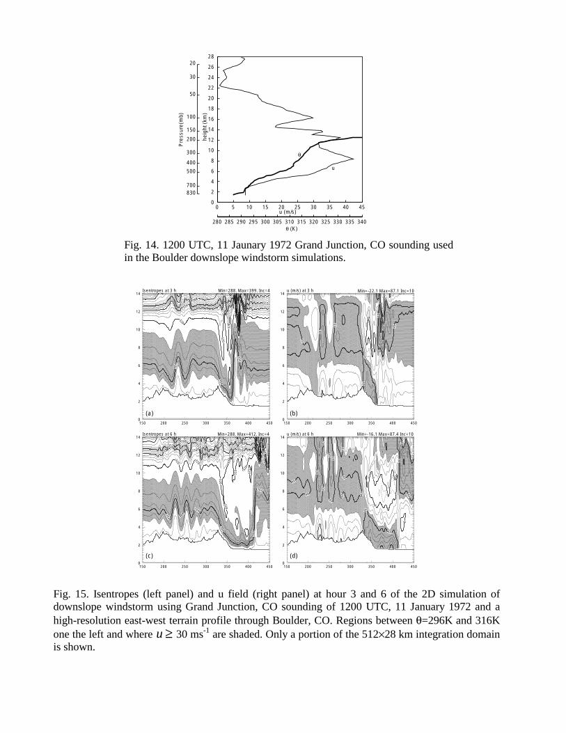
u (m/s)0 5 10 15 20 25 30 35 40 45

0

2

4

6

8

10

12

14

16

18

20

22

24

26

28

heig

ht (

km)

830700

500

400

300

200

150

100

50

30

20

Pre

ssur

e(m

b)

θ (K)280 285 290 295 300 305 310 315 320 325 330 335 340

θ

u

Fig. 14. 1200 UTC, 11 Jaunary 1972 Grand Junction, CO sounding used in the Boulder downslope windstorm simulations.

304

304

304

320

320

320

320

336

336

352 352

352368

150 200 250 300 350 400 4500

2

4

6

8

10

12

14Min=288. Max=399. Inc=4Isentropes at 3 h

0

40

40

40

40

40

40

40

150 200 250 300 350 400 4500

2

4

6

8

10

12

14Min=-22.1 Max=87.1 Inc=10u (m/s) at 3 h

304 304

304

304

304

304

320

320

320320

320

320 32

0

320

320

336 336

336 336

336

352 352 352 352

352368

368

368

384

150 200 250 300 350 400 4500

2

4

6

8

10

12

14Min=288. Max=412. Inc=4Isentropes at 6 h

0

00

0

0

40

40

40

40

40

40

40

40

40

40

4040

40

40

40

40

40

150 200 250 300 350 400 4500

2

4

6

8

10

12

14Min=-16.1 Max=87.4 Inc=10u (m/s) at 6 h

(a)

(d)

(b)

(c)

Fig. 15. Isentropes (left panel) and u field (right panel) at hour 3 and 6 of the 2D simulation of downslope windstorm using Grand Junction, CO sounding of 1200 UTC, 11 January 1972 and a

high-resolution east-west terrain profile through Boulder, CO. Regions between θ=296K and 316K

one the left and where u 30 ms-1 are shaded. Only a portion of the 512×28 km integration domain

is shown.

0.0 3.2 6.4 9.6 12.8 16.00.0

0.8

1.6

2.4

3.2

4.0

4.8Min=-16.6 Max=0. Inc=1.0

0.0 3.2 6.4 9.6 12.8 16.00.0

0.8

1.6

2.4

3.2Min=-11.4 Max=0.0 Inc=1.0

0.0 3.2 6.4 9.6 12.8 16.00.0

0.8

1.6

2.4Min=-9.68 Max=0.0 Inc=1.0

θ' 0s

REF25

θ' 900s

REF25

θ' 600s

REF25

(c)

(a)

(b)

Fig. 16. θ' contours from the 25 m resolution reference simulation, at (a) 0, (b) 600, and (c) 900 s. Contour interval is 1°C. Only a portion of the 25.6×6.4 km2

domain is shown. The figure shows that an oval shaped initial cold blob drops to the ground and spread along the ground in the form of density current. Kelvin-Helmholtz billows develop along the upper surface the cold pool.

0.0 3.2 6.4 9.6 12.8 16.00.0

0.8

1.6

2.4Min=-17.1 Max=1.89 Inc=1.0

0.0 3.2 6.4 9.6 12.8 16.00.0

0.8

1.6

2.4Min=-14.1 Max=2.26 Inc=1.0

0.0 3.2 6.4 9.6 12.8 16.00.0

0.8

1.6

2.4Min=-7.62 Max=0.0 Inc=1.0

0.0 3.2 6.4 9.6 12.8 16.00.0

0.8

1.6

2.4Min=-7.00 Max=0.0 Inc=1.0

0.0 3.2 6.4 9.6 12.8 16.00.0

0.8

1.6

2.4Min=-8.94 Max=0.0 Inc=1.0

θ' 2nd400

θ' REF400

θ' FCT2nd400

θ' 4th400

θ' FCT4th400

(d)

(a)

(b)

(c)

(e)

Fig. 17. Fields of θ' at 900 s from the 400 m resolution experiments (a) 2nd400, (b) 4th400, (c) FCT400, (d) MP400 and (e) the 25 m reference run. The reference solution has been averaged to the 400 m grid.

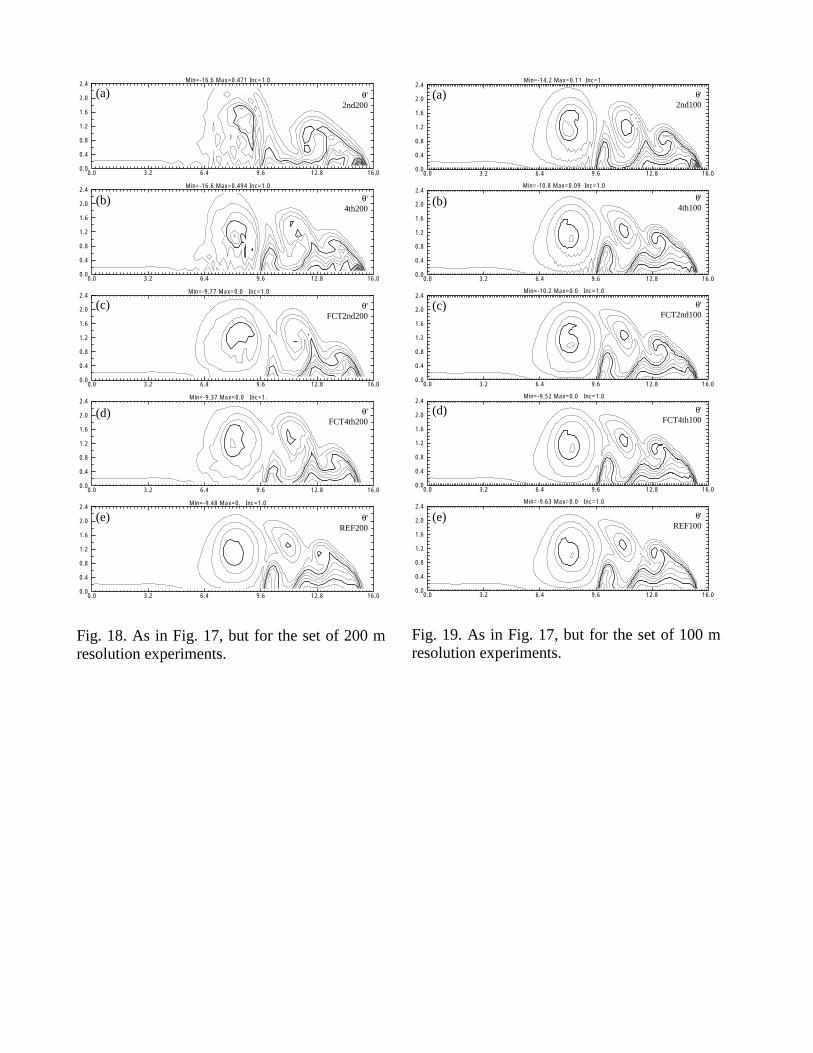
0.0 3.2 6.4 9.6 12.8 16.00.0

0.4

0.8

1.2

1.6

2.0

2.4Min=-16.6 Max=0.471 Inc=1.0

0.0 3.2 6.4 9.6 12.8 16.00.0

0.4

0.8

1.2

1.6

2.0

2.4Min=-16.6 Max=0.494 Inc=1.0

0.0 3.2 6.4 9.6 12.8 16.00.0

0.4

0.8

1.2

1.6

2.0

2.4Min=-9.77 Max=0.0 Inc=1.0

0.0 3.2 6.4 9.6 12.8 16.00.0

0.4

0.8

1.2

1.6

2.0

2.4Min=-9.37 Max=0.0 Inc=1.

0.0 3.2 6.4 9.6 12.8 16.00.0

0.4

0.8

1.2

1.6

2.0

2.4Min=-9.48 Max=0. Inc=1.0

θ' 2nd200

θ' REF200

θ' FCT2nd200

θ' 4th200

θ' FCT4th200

(d)

(a)

(b)

(c)

(e)

Fig. 18. As in Fig. 17, but for the set of 200 m resolution experiments.

0.0 3.2 6.4 9.6 12.8 16.00.0

0.4

0.8

1.2

1.6

2.0

2.4Min=-14.2 Max=0.11 Inc=1.

0.0 3.2 6.4 9.6 12.8 16.00.0

0.4

0.8

1.2

1.6

2.0

2.4Min=-10.8 Max=0.09 Inc=1.0

0.0 3.2 6.4 9.6 12.8 16.00.0

0.4

0.8

1.2

1.6

2.0

2.4Min=-10.2 Max=0.0 Inc=1.0

0.0 3.2 6.4 9.6 12.8 16.00.0

0.4

0.8

1.2

1.6

2.0

2.4Min=-9.52 Max=0.0 Inc=1.0

0.0 3.2 6.4 9.6 12.8 16.00.0

0.4

0.8

1.2

1.6

2.0

2.4Min=-9.63 Max=0.0 Inc=1.0

(d)

(a)

(b)

(c)

(e)

θ' 2nd100

θ' REF100

θ' FCT2nd100

θ' 4th100

θ' FCT4th100

Fig. 19. As in Fig. 17, but for the set of 100 m resolution experiments.