The Analysis and Utilization of Cycling Training Data · The Analysis and Utilization of Cycling Training Data Simon A. Jobson,1 Louis Passfield,1 Greg Atkinson,2 Gabor Barton2 and

The Analysis and Utilizationof Cycling Training DataSimon A. Jobson,1 Louis Passfield,1 Greg Atkinson,2 Gabor Barton2 and Philip Scarf 3

1 Centre for Sports Studies, University of Kent, Chatham, Kent, UK

2 Research Institute for Sport and Exercise Science, Liverpool John Moores University, Liverpool, UK

3 Centre for OR and Applied Statistics, University of Salford, Salford, UK

Contents

Abstract. . . . . . . . . . . . . . . . . . . . . . . . . . . . . . . . . . . . . . . . . . . . . . . . . . . . . . . . . . . . . . . . . . . . . . . . . . . . . . . . . 8331. Quantification of Training . . . . . . . . . . . . . . . . . . . . . . . . . . . . . . . . . . . . . . . . . . . . . . . . . . . . . . . . . . . . . . . 834

1.1 Session Rating of Perceived Exertion . . . . . . . . . . . . . . . . . . . . . . . . . . . . . . . . . . . . . . . . . . . . . . . . . . 8341.2 Ordinal Categorization . . . . . . . . . . . . . . . . . . . . . . . . . . . . . . . . . . . . . . . . . . . . . . . . . . . . . . . . . . . . . 8351.3 Heart Rate Recovery and Training Impulse. . . . . . . . . . . . . . . . . . . . . . . . . . . . . . . . . . . . . . . . . . . . . 8351.4 Excess Post-Exercise Oxygen Consumption . . . . . . . . . . . . . . . . . . . . . . . . . . . . . . . . . . . . . . . . . . . . 8351.5 Power Output . . . . . . . . . . . . . . . . . . . . . . . . . . . . . . . . . . . . . . . . . . . . . . . . . . . . . . . . . . . . . . . . . . . . . 836

1.5.1 Average Power . . . . . . . . . . . . . . . . . . . . . . . . . . . . . . . . . . . . . . . . . . . . . . . . . . . . . . . . . . . . . . 8371.5.2 Normalized Power . . . . . . . . . . . . . . . . . . . . . . . . . . . . . . . . . . . . . . . . . . . . . . . . . . . . . . . . . . . . 837

1.6 Power Spectrum Analysis. . . . . . . . . . . . . . . . . . . . . . . . . . . . . . . . . . . . . . . . . . . . . . . . . . . . . . . . . . . . 8372. Modelling the Relationship between Training and Performance . . . . . . . . . . . . . . . . . . . . . . . . . . . . . . 838

2.1 Impulse-Response Models . . . . . . . . . . . . . . . . . . . . . . . . . . . . . . . . . . . . . . . . . . . . . . . . . . . . . . . . . . . 8382.2 Neural Networks . . . . . . . . . . . . . . . . . . . . . . . . . . . . . . . . . . . . . . . . . . . . . . . . . . . . . . . . . . . . . . . . . . . 8392.3 Dynamic Meta-Model . . . . . . . . . . . . . . . . . . . . . . . . . . . . . . . . . . . . . . . . . . . . . . . . . . . . . . . . . . . . . . 8402.4 Multiple Regression and Mixed Linear Modelling . . . . . . . . . . . . . . . . . . . . . . . . . . . . . . . . . . . . . . . . 8402.5 Cluster Analysis . . . . . . . . . . . . . . . . . . . . . . . . . . . . . . . . . . . . . . . . . . . . . . . . . . . . . . . . . . . . . . . . . . . . 8412.6 Non-Linear Dynamics and Chaos Theory . . . . . . . . . . . . . . . . . . . . . . . . . . . . . . . . . . . . . . . . . . . . . . 841

3. Conclusions . . . . . . . . . . . . . . . . . . . . . . . . . . . . . . . . . . . . . . . . . . . . . . . . . . . . . . . . . . . . . . . . . . . . . . . . . . . 841

Abstract Most mathematical models of athletic training require the quantificationof training intensity and quantity or ‘dose’. We aim to summarize both themethods available for such quantification, particularly in relation to cyclesport, and the mathematical techniques that may be used to model the re-lationship between training and performance.

Endurance athletes have used training volume (kilometres per week and/orhours per week) as an index of training dose with some success. However,such methods usually fail to accommodate the potentially important influ-ence of training intensity. The scientific literature has provided some supportfor alternative methods such as the session rating of perceived exertion, whichprovides a subjective quantification of the intensity of exercise; and the heartrate-derived training impulse (TRIMP) method, which quantifies the train-ing stimulus as a composite of external loading and physiological re-sponse, multiplying the training load (stress) by the training intensity (strain).

REVIEW ARTICLESports Med 2009; 39 (10): 833-8440112-1642/09/0010-0833/$49.95/0

ª 2009 Adis Data Information BV. All rights reserved.

Othermethods described in the scientific literature include ‘ordinal categoriza-tion’ and a heart rate-based excess post-exercise oxygen consumption method.

In cycle sport, mobile cycle ergometers (e.g. SRM� and PowerTap�) arenow widely available. These devices allow the continuous measurement of thecyclists’ work rate (power output) when riding their own bicycles during trainingand competition.However, the inherent variability in power output when cyclingposes several challenges in attempting to evaluate the exact nature of a session.Such variability means that average power output is incommensurate with thecyclist’s physiological strain. A useful alternative may be the use of an exponen-tially weighted averaging process to represent the data as a ‘normalized power’.

Several research groups have applied systems theory to analyse the responsesto physical training. Impulse-response models aim to relate training loads toperformance, taking into account the dynamic and temporal characteristics oftraining and, therefore, the effects of load sequences over time. Despite thesuccesses of this approach it has some significant limitations, e.g. an excessivenumber of performance tests to determine model parameters. Non-linear arti-ficial neural networks may provide a more accurate description of the complexnon-linear biological adaptation process. However, such models may also beconstrained by the large number of datasets required to ‘train’ the model.

A number of alternative mathematical approaches such as the Perfor-mance-Potential-Metamodel (PerPot), mixed linear modelling, cluster anal-ysis and chaos theory display conceptual richness. However, much furtherresearch is required before such approaches can be considered as viable al-ternatives to traditional impulse-response models. Some of these methodsmay not provide useful information about the relationship between trainingand performance. However, they may help describe the complex physiologi-cal training response phenomenon.

Scientists examining exercise training haveidentified distinct roles for training volume, in-tensity and frequency in the adaptation process.[1]

In order to optimize performance when workingwith elite athletes, it is essential that the sportscoach has a thorough understanding of the re-lationship between training and performance.These relationships have been shown to be highlyindividualized due to variation in factors such asindividual training background,[2] genetics[3] andpsychological factors.[4] In order to further thisunderstanding, a number of mathematical modelshave been developed in an attempt to describe thedynamic aspect of training and the consequencesof successive training loads over time.[4-6]

1. Quantification of Training

Most mathematical models of athletic trainingrequire the quantification of training intensity

and quantity or ‘dose’. Ideally, this quantifica-tion requires researchers to incorporate para-meters for intensity, duration and frequency.Endurance athletes have used training volume(kilometres per week and/or hours per week) asan index of training dose with some success.[7,8]

However, this index fails to accommodate thepotentially important influence of training inten-sity. Therefore, a number of alternative methodshave been investigated.

1.1 Session Rating of Perceived Exertion

The rating of perceived exertion (RPE) pro-vides one method of subjectively quantifying theintensity of exercise.[9] Defined by the intensity ofdiscomfort or fatigue felt at a particular moment,RPE has been shown to correlate well with inten-sity of effort.[10] In order to provide an index of awhole training session, Foster et al.[11] developed

834 Jobson et al.

ª 2009 Adis Data Information BV. All rights reserved. Sports Med 2009; 39 (10)

the session RPE (sRPE) scale as a modification ofthe standard RPE scale. Rather than providingan RPE score for a specific aspect (e.g. interval/set) of an exercise session, sRPE aims to providean RPE for the session as a whole, i.e. to integratethe myriad of exercise-intensity cues.[10] ThesRPE scale has been shown to be a reliable andvalid method of quantifying intensity during bothaerobic and resistance exercise when comparedwith heart rate-based metrics.[10,12,13]

1.2 Ordinal Categorization

Training has also been categorized into or-dinal levels based on differences in intensity.Whilst this categorization has been arbitrary insome instances,[14] this approach is commonlybased upon the relationship between a measuredvariable, such as speed, and heart rate[15] or lac-tate response.[2] Each category is then assigned anarbitrary weighting coefficient that emphasizeshigh-intensity training sessions. Being basedupon an individual’s physiological response andassuming a non-linear response to increasing ex-ercise intensity, these methods appear more sci-entifically defendable. However, an element ofsubjectiveness remains due to the arbitraryweighting of intensity categories. Furthermore,using heart rate in the process of training quan-tification has a number of limitations. Irrespec-tive of exercise intensity, heart rate may vary dueto factors such as cardiac drift,[16] changes intemperature,[17] hydration status and body posi-tion on the bicycle.[16]

1.3 Heart Rate Recovery and Training Impulse

Overcoming some of the above limitations,Borresen and Lambert[18,19] have suggested that, asindirect markers of autonomic function, heart ratevariability and, in particular, heart rate recoverymay offer practical ways of quantifying the phy-siological effects of training. However, much fur-ther work is required before these methods can beshown to have practical application in the pre-scription of optimal training programmes.[19]

Training impulse (TRIMP) quantifies thetraining stimulus as a composite of external

loading and physiological response, multiplyingthe training load (stress) by the training intensity(strain).[20] Banister and Calvert’s[21] originalformula was modified by Morton et al.[22] to in-clude a multiplicative factor that gave greaterweight to high-intensity training (equation 1):

TRIMP ¼ exercise duration �

fraction of heart rate reserve �

eðfraction of heart rate reserve � bÞðEq: 1Þ

where e is Euler’s number, 2.718, and b is a con-stant based on the blood lactate response duringincremental exercise and is equal to 1.92 in malesand 1.67 in females.

There are advantages to using the TRIMPmethod, evidenced not least by the number ofresearchers who have explored the use of thismetric.[23-25] It is relatively easy to calculate TRIMPwith an inexpensive and commonly used heartrate monitor. This approach produces a singlenumber that represents the training stimulus pro-vided by the whole session. However, the originalBanister formulation of the TRIMP concept failedto take into account the energy system-specificeffects of training intensity. Whilst, to some ex-tent, Morton’s weighting factor overcomes thisshortcoming, it is still limited in assuming afixed relationship between heart rate and lactateresponses; an assumption that Hurley et al.[26]

dispute.

1.4 Excess Post-Exercise Oxygen Consumption

Whilst sRPE and TRIMP have received sup-port in the scientific literature, both methods arelimited by a lack of underpinning physiologicaltheory. In order to quantify the homeostatic dis-turbance associated with training, traditionalphysiological measures such as oxygen consump-tion, heart rate and blood lactate may be obtained.However, these latter measures only reflect amomentary response to exercise. Blood lactateconcentration, measured during or post-exercise,might also depend on sampling site. In contrast,the measurement of excess post-exercise oxygenconsumption (EPOC) has been suggested to re-flect the cumulative response of the body to awhole training session. As with the measurement

Analysing Cycling Training Data 835


of oxygen uptake and lactate response, EPOCassessment is laboratory-based, expensive, time-consuming and, therefore, inappropriate for reg-ular assessment.Recognizing this limitation, Ruskoet al.[27] developed a heart rate-based EPOC (HR-based EPOC) prediction model, which is mathe-matically described as equation 2:

EPOCðtÞ ¼ fðEPOCðt�1Þ; % V:O2max; DtÞ ðEq: 2Þ

EPOC at time t (EPOC(t)) is estimated using thevariables of current intensity (%

.VO2max), dura-

tion of exercise (time between two samplingpoints [Dt]) and EPOC in the previous sampl-ing point (EPOC(t–1)). This model has been vali-dated in a group of 32 healthy adult subjects,HR-based EPOC correlating well with measuredEPOC (r = 0.89).[27] Mean absolute error valuesfor the HR-based EPOC, when compared withthe measured EPOC values, were 9.4, 14.0 and16.9mL/kg for 40% and 70% constant load ex-ercise and for maximal incremental exercise, re-spectively. However, despite the attractiveness ofthis model, the calculation is relatively complex,currently requiring proprietary software andhardware (e.g. Suunto� t6 heart rate monitor).In addition, the model has only been validated inone study, in which only short-duration exercise(2 · 10min) was investigated.[27]

1.5 Power Output

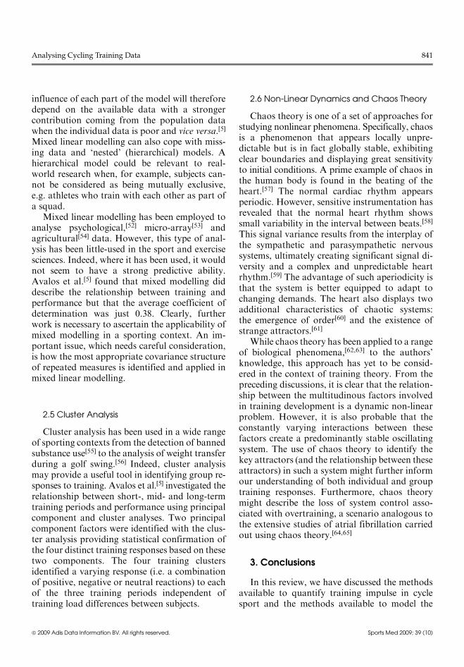
Mobile cycle ergometers (e.g. SRM� andPowerTap�) are now widely available and allowthe continuous measurement of the cyclists’ workrate (power output) when riding their own bi-cycles during training and competition. Indeed,in one study of these devices, the authors con-cluded, ‘‘measures with such low error mightbe suitable for tracking the small changes incompetitive performance that matter to elite cy-clists.’’[28] Consequently, these devices have beenwidely used by elite cyclists during training andcompetition. Thus, with such instrumented bi-cycles it is now possible to examine the completedtraining and race performances and associatedphysiological responses in detail. An example oftypical data collected during a training bout isshown in figure 1. This ability to accurately

quantify the mechanical work of training, as wellas the detail and extent of these data, makes cy-cling unique in allowing such insight into the de-mands of sporting preparation and competition.However, it can also be seen that the inherentvariability in power output during training posesseveral challenges in attempting to evaluate theexact nature of any training session.

As a result of the difficulties in interpretationof power output data, the current practice formany athletes and coaches is to simply visuallyinspect individual training sessions (e.g. as pre-sented in figure 1). In this way, general features ofthe session may be identified, such as the point atwhich the highest power output was achieved, thenumber of intervals completed or the level ofpower output variation. Clearly, such methodsfail to allow full analysis of the available data. Analternative approach is to evaluate the amount oftime spent within given power ‘bins’ or ‘zones’using a histogram. Ebert et al.[29] provided agraphical comparison of two types of women’sWorld Cup cycle road races by evaluating thepercentage of total race time spent within fourpower bins (0–100W, 100–300W, 300–500Wand >500W). Recognizing the important influ-ence of body mass on cycling performance, Ebertet al.[30] provided similar comparisons of poweroutput per unit body mass (W/kg) in a group ofprofessional male stage race cyclists. Althoughsimple, this method is excellent for the purpose ofoverall session comparisons.[31] However, the histo-gram approach is limited by its inability to recogn-ize separate efforts within any given power zone.

700

600

500

400

300

200

100

0

Pow

er o

utpu

t (W

)

00:00 00:30 01:00 01:30 02:00 02:30 03:00 03:30 04:00

Time (h:min)

Fig. 1. Example of training power output data measured with anSRM� crank system.

836 Jobson et al.


For example, this method is unable to differentiatebetween a single 5-minute effort at 350W and five1-minute intervals at the same intensity, althoughthe effect of these two bouts of exercise on train-ing outcomes may be very different.[32]

1.5.1 Average Power

Power output provides a direct and immediatemeasure of work rate, as opposed to the athlete’sperceptual or cardiovascular response to thatexercise intensity. However, as discussed in sec-tion 1.5, the stochastic nature of work rate whencycling outdoors[33] makes interpretation of in-formation from on-bike power meters proble-matic. A simple approach is to calculate mean oraverage power over the duration of the trainingbout. However, average power is not necessarilycommensurate with the cyclist’s physiologicalstrain unless the training session is constantpower in nature. For example, a maximum effortin a 1-hour time-trial over flat terrain may resultin a mean power of 299W and require little var-iation in power output over the course of the race(figure 2a). In contrast, a maximum effort re-quiring marked changes of pace, e.g. in a criter-ium-type race or a hilly time-trial, may result inthe rider being able to produce a much loweraverage of only 260W (figure 2b). Future re-search should seek to describe in detail what thedifferences in overall power are for variable ver-sus constant power cycling.

1.5.2 Normalized Power

Recognizing the limitations of the averagepower approach, Coggan[34] has proposed usingan exponentially weighted averaging process torepresent the data. Data are smoothed using a30-second moving average (because many physio-logical processes [e.g. V

:O2, heart rate] respond to

changes in exercise intensity with a time-constantof ~30 s) before being raised to the fourth power(derived from a regression of blood lactate con-centration against exercise intensity). Finally, thetransformed values are averaged and the fourthroot taken, yielding a ‘normalized power’. Usingthis process, it is theoretically possible to makemore direct comparisons between different types

of training sessions. In the above example, forinstance, the time-trial effort normalized remainsabout 299W (figure 2a), but the variable effort of260W normalized becomes 291W (figure 2b).Whilst this method has attracted substantial in-terest from the cycling community, it has as yetreceived very little critical evaluation from thescientific community.[35]

1.6 Power Spectrum Analysis

The ability to move forward during cyclingrequires energy to overcome environmental resis-tance (principally wind, rolling and gravitationalresistance[36]). Thus, variation in these resistiveforces whilst cycling results in predictable changesin power output. However, beyond these physicalrelationships, Hu et al.[37] have suggested that

500a

450400350300250200

Pow

er o

utpu

t (W

)

150100500

0 10 20 30

Time (min)

40 50 60

500b

450400350300250200

Pow

er o

utpu

t (W

)

150100500

0 10 20 30

Time (min)

40 50 7060

Fig. 2. 30-second rolling average for power for a flat time-trial (a)and a criterium road race (b) performed by the same cyclist. Notethat average power (dashed line) varies widely between efforts,whilst the normalized power (solid line) is similar, indicating anequivalent physiological cost for both efforts.



‘other’ fluctuations in data from biological systemsrepresent ‘noise’, this being the result of eitherrandom processes or external input to the system.If this noise was the result of random factors, apower spectrum analysis would reveal a Gaussianwhite noise signal (i.e. where all frequencies havean equal power weighting).[38] Tucker et al.[39] useda discrete Fourier transform (DFT) in order to eval-uate the power spectrum of the power output ofamateur cyclists. A DFT expresses data as a sumof sinusoidal waveforms of varying frequency(figure 3), with the spectrum of the signal beingthe signal that describes the way in which theamplitudes and phases of these waveformschange with frequency. Therefore, at a specificfrequency it is possible to obtain the measure ofthe contribution that a specific waveform willmake to the signal. Using this method, Tucker etal.[39] demonstrated the presence of dominantfrequency peaks (at distance cycles of ~2.5, ~6,~12 and ~21km) during a laboratory-based 20kmtime-trial, suggesting that the observed poweroutput fluctuations were in fact non-random.Tucker et al.[39] proposed that the fluctuations inpower output were the result of the regulation ofpower output by intrinsic biological control pro-cesses. Differing dominant frequency spikes werealso observed when analysing the frequencyspectrum of individual components of the time-trial (i.e. beginning, middle and end) and the trial

as a whole. Each of these dominant spikes wassuggested to represent a different control systemor component of an overall system. It wouldbe interesting to investigate if such effects arerepeated in a larger dataset and over longer per-iodicities (e.g. days, months) than those con-sidered by these authors.

Tucker et al.[39] also investigated the level ofself-similarity in the time-trial power output signalof cyclists using a fractal analysis. In this context,the concept of self-similarity refers to the propertythat parts of the fractal signal are similar to thewhole. Despite the large variability in power out-put generated both inter- and intra-trial, these au-thors found that the fractal dimension of the powerspectrum was similar (1.56–1.9) in all subjects.Thus, despite the irregular power spectrum signal,there would appear to be a degree of self-similaritybetween parts of the signal and the signal as awhole. Tucker et al.[39] suggested that this signalconcordance indicates a similar overall controllingprocess present in each cyclist and throughout eachtime-trial. Further research should seek to estab-lish whether such findings reflect real physiologicalphenomena or, instead, if they simply reflect thewidespread applicability of fractals.

2. Modelling the Relationship betweenTraining and Performance

Models may be purely empirical or basedon a detailed appreciation of the underlyingstructure.[20] Clearly, these underlying structurescan be extremely complex. Whilst mathematicalmodels are based on abstractions of the real sys-tem, the question remains of how much under-lying structure to incorporate into models oftraining and performance.

2.1 Impulse-Response Models

Building upon early investigations by Banisteret al.,[4] several research groups have appliedsystems theory to analyse the responses to physi-cal training.[2,40,41] This approach attempts to ab-stract a dynamic process into amathematicalmodel,the system being characterized by at least oneinput and one output related by a mathematical

86420

0 4 8

Distance (km)

12 16 20

−10−8−6−4−2

Pow

er m

ean

1 cycle/20 km2 cycles/20 km3 cycles/20 kmSum

Fig. 3. An example of a Fourier transformation expressing the dataas a sum of sinusoidal waveforms of varying frequency. In this ex-ample, three sinusoidal waveforms were added together to create apower signal that looks similar to the power output data observedduring a 20 km time-trial (reproduced from Tucker et al.,[39] withpermission).

838 Jobson et al.


‘transfer function’.[42] This function follows thegeneral form (equation 3):

Model performance ¼ ðfitness from trainingmodelÞ �

Kðfatigue from trainingmodelÞ

ðEq: 3Þ

where K is the constant that adjusts for themagnitude of the fatigue effect relative to the fit-ness effect.[20] Calvert et al.[14] presented a simplemodel whereby a single training impulse elicitedtwo fitness responses that would increase perfor-mance and a fatigue response that would decreaseperformance. Thus, ‘impulse-response’ modelsaim to relate training loads to performance, tak-ing into account the dynamic and temporalcharacteristics of training and, therefore, theeffects of load sequences over time.

This model has been presented in a variety ofmathematical forms, most notably the differ-ential equations of Calvert et al.,[14] Mortonet al.,[22] Busso et al.[43] Fitz-Clarke et al.[44] andBusso et al.[45] have built upon these formulationsto present influence curves that provide a clearpicture of how a specific training session affectsperformance at a future time. Indeed, Bussoet al.[45] found that the positive and negative ‘in-fluences’ (PI and NI) were actually closer to thevariations in performance than the values calcu-lated by the positive and negative functions (PFand NF) produced in the underlying mathema-tical model itself (i.e. where PF and NF representan immediate fitness gain and PI and NI re-present a more biologically plausible delayed fit-ness gain).

A variety of data types have been used as inputin impulse-response type models. When predict-ing the performance of two non-elite runners,Morton et al.[22] quantified training impulse usingTRIMPs. In one subject, agreement betweenmeasured and predicted performance was ex-cellent (R2 = 0.96), whilst in the second it was lessimpressive (R2 = 0.71). Through the utilization ofordinal categorization of training, Mujika et al.[2]

identified weaker relationships, with the explainedvariation in performance ranging from R2 = 0.45to R2 = 0.85 in a group of elite swimmers. Oneproposed explanation for this variability is thatmodel parameters change over time (i.e. with

training). As such, Busso et al.[46] compared botha time-varying and a time-invariant model, withR2 = 0.88 and R2 = 0.68, respectively. However,the use of the model and its parameters to predictthe responses to future training is precludedwith the time-varying approach, unless the para-meters change in a predictable manner.[20]

Impulse-response modelling provides pertinentinformation about interindividual differences andpermits the construction of individualized train-ing programmes[47] (e.g. TRIMP, TrainingPeaksWKO+ and RaceDay software). However, boththe original Banistermodel and its extensions havesome significant limitations. Taha and Thomas[20]

argued that the model does not correspond withcontemporary understanding of physiologicalmechanisms, requires an excessive number of per-formance tests to determine model parameters,and is unable to distinguish the specific effects ofdifferent training impulses. Furthermore, inter-study and inter-subject variability in parameterestimates limits the ability to apply a genericversion of the model.

2.2 Neural Networks

Traditional impulse-response models such asthose described in section 2.1 are based on linearmathematical concepts such as regression analy-sis and linear differential equations. However,because the adaptation of a biological systemleads to changes in the system itself, biologicaladaptation is actually a complex non-linear pro-blem.[48] For this reason, Edelmann-Nusseret al.[48] used a non-linear multi-layer perceptronneural network to model the performance of anOlympic-level swimmer. This model produced a‘prediction error’ of just 0.04%.

One problem associated with neural networksis that they typically require many datasets to‘train’ the model. Having ten input neurons, twohidden neurons and one output neuron, trainingof the model used by Edelmann-Nusser et al.[48]

required 40 datasets (this number increasing to60 with the addition of just one neuron in thehidden layer). Thus, it may be some time beforesuch a model becomes useful for any given ath-lete. Edelmann-Nusser et al.[48] overcame this



problem by training the model with the datasetsof another athlete. Ultimately, this methodproved to be successful, but, as noted by the au-thors, it may have been fortuitous that theadaptive behaviour of both athletes was similar.Although the predictive power is impressive,Hellard et al.[47] have cautioned that the majorweakness of neural network models is that theydon’t explicitly identify causal relationships,i.e. they function as a ‘black box’.

2.3 Dynamic Meta-Model

The Performance-Potential-Metamodel (Per-Pot) described by Perl[6] simulates the interactionbetween load and performance interaction bymeans of antagonistic dynamics. Hellard et al.[47]

highlighted the conceptual richness of this modelin that it accounts for the collapse effect in thewake of training overload, the atrophy associatedwith detraining and the long-term behaviour ofthe training-performance relationship.

Similar to the Banister model, the basic con-cept of the PerPot model is that of antagonism(see figure 4). Each load impulse feeds a strainpotential as well as a response potential. Thesebuffer potentials in turn influence the perfor-mance potential, where the response potentialraises the performance potential (delayed by thedelay in response flow) and the strain potential

reduces the performance potential (delayed bythe delay in strain flow). If the strain potential isoverloaded an overflow is produced that has afurther negative impact on performance poten-tial. Whilst this model is attractive, to the au-thors’ knowledge no researcher has yet provideda critical validation.

2.4 Multiple Regression and Mixed LinearModelling

As described above (section 2.1), one of theproblems associated with the Banister model isthe need for a very large number of datapointsper parameter. To ensure a stable solution in aregression analysis, Stevens[49] recommended aminimum of 15 observations per predictor vari-able. To avoid these difficulties multiple regres-sion modelling has been suggested as a viable al-ternative, especially when relatively few repeatedmeasurements are available for multiple sub-jects.[47] This method allows the integrationof training loads as independent variables andcan take the effects of load sequences over timeinto account. Mujika et al.[50] used a stepwise re-gression to create a model for the relationshipbetween training and performance, reporting avery close match with the Banister model.

Mixed linear modelling can be applied to re-peated measures data from unbalanced designs(i.e. multiple independent variables with un-balanced multiple levels on each factor). Unlikethe Banister model, which produces a personalmodel for each subject, mixed models accom-modate subject heterogeneity by allowing para-meters to vary between individuals as a model ofpopulation behaviour is constructed.[5] There-fore, this type of analysis can also cope with themixture of random and fixed effects that occurwith ‘real-world’ data.[51] For example, perfor-mance-related data might be influenced by ran-dom fluctuations in environmental factors as wellas systematic changes to training that are intro-duced by the coach. In general, all data are usedto construct the part of the model common to thewhole subject population whilst only the observa-tions specific to each individual are used to con-struct the personal part of the model. The relative

Load

Responsepotential

Strainpotential

DS DR

Performance potential

+

++

−

Fig. 4. Antagonistic structure of the Performance-Potential-Meta-model. DR = delay in response flow; DS = delay in strain flow.

840 Jobson et al.


influence of each part of the model will thereforedepend on the available data with a strongercontribution coming from the population datawhen the individual data is poor and vice versa.[5]

Mixed linear modelling can also cope with miss-ing data and ‘nested’ (hierarchical) models. Ahierarchical model could be relevant to real-world research when, for example, subjects can-not be considered as being mutually exclusive,e.g. athletes who train with each other as part ofa squad.

Mixed linear modelling has been employed toanalyse psychological,[52] micro-array[53] andagricultural[54] data. However, this type of anal-ysis has been little-used in the sport and exercisesciences. Indeed, where it has been used, it wouldnot seem to have a strong predictive ability.Avalos et al.[5] found that mixed modelling diddescribe the relationship between training andperformance but that the average coefficient ofdetermination was just 0.38. Clearly, furtherwork is necessary to ascertain the applicability ofmixed modelling in a sporting context. An im-portant issue, which needs careful consideration,is how the most appropriate covariance structureof repeated measures is identified and applied inmixed linear modelling.

2.5 Cluster Analysis

Cluster analysis has been used in a wide rangeof sporting contexts from the detection of bannedsubstance use[55] to the analysis of weight transferduring a golf swing.[56] Indeed, cluster analysismay provide a useful tool in identifying group re-sponses to training. Avalos et al.[5] investigated therelationship between short-, mid- and long-termtraining periods and performance using principalcomponent and cluster analyses. Two principalcomponent factors were identified with the clus-ter analysis providing statistical confirmation ofthe four distinct training responses based on thesetwo components. The four training clustersidentified a varying response (i.e. a combinationof positive, negative or neutral reactions) to eachof the three training periods independent oftraining load differences between subjects.

2.6 Non-Linear Dynamics and Chaos Theory

Chaos theory is one of a set of approaches forstudying nonlinear phenomena. Specifically, chaosis a phenomenon that appears locally unpre-dictable but is in fact globally stable, exhibitingclear boundaries and displaying great sensitivityto initial conditions. A prime example of chaos inthe human body is found in the beating of theheart.[57] The normal cardiac rhythm appearsperiodic. However, sensitive instrumentation hasrevealed that the normal heart rhythm showssmall variability in the interval between beats.[58]

This signal variance results from the interplay ofthe sympathetic and parasympathetic nervoussystems, ultimately creating significant signal di-versity and a complex and unpredictable heartrhythm.[59] The advantage of such aperiodicity isthat the system is better equipped to adapt tochanging demands. The heart also displays twoadditional characteristics of chaotic systems:the emergence of order[60] and the existence ofstrange attractors.[61]

While chaos theory has been applied to a rangeof biological phenomena,[62,63] to the authors’knowledge, this approach has yet to be consid-ered in the context of training theory. From thepreceding discussions, it is clear that the relation-ship between the multitudinous factors involvedin training development is a dynamic non-linearproblem. However, it is also probable that theconstantly varying interactions between thesefactors create a predominantly stable oscillatingsystem. The use of chaos theory to identify thekey attractors (and the relationship between theseattractors) in such a system might further informour understanding of both individual and grouptraining responses. Furthermore, chaos theorymight describe the loss of system control asso-ciated with overtraining, a scenario analogous tothe extensive studies of atrial fibrillation carriedout using chaos theory.[64,65]

3. Conclusions

In this review, we have discussed the methodsavailable to quantify training impulse in cyclesport and the methods available to model the



relationship between this training impulse andperformance. Many of the methods discussed areapplicable across a wide range of sports; how-ever, cycling is one of the few sports able to takeadvantage of the rich data provided by the conti-nuous measurement of work rate (power output).

Individual training/competition bouts may bequantified using methods such as sRPE, TRIMPandHR-based EPOC. Themeasurement of poweroutput enables sessions to be quantified in a num-ber of ways that include histogram approaches,mean power output and ‘normalized power’ output.While different (useful) information is conveyedby each approach, further research should seek toprovide a direct comparison of these methods.

A number of mathematical approaches havebeen used to analyse the responses to physicaltraining. The use of impulse-response models hasreceived substantial support in the scientific lit-erature, whilst alternative approaches such as thePerPot metamodel and mixed linear modellinghave yet to be fully explored. The type of analysisthat a researcher/coach uses will depend upon thenumber of datapoints available, with the morecomplex models requiring more measurementsbeing made over time. It is likely that some of themethods discussed here will not provide usefulinformation when describing the relationshipbetween training and performance. However,it is probable that some combination of theseapproaches, rather than any single model, willprovide the best description of the complex phy-siological training response phenomenon.

Acknowledgements

The preparation of this manuscript was supported withfunding from the Engineering and Physical Sciences ResearchCouncil, UK. The authors have no conflicts of interest thatare directly relevant to the content of this review.

References1. Godfrey R, Whyte G. Training specificity. In: Whyte G,

editor. The physiology of training. London: ChurchillLivingstone Elsevier, 2006: 23-43

2. Mujika I, Busso T, Lacoste L, et al. Modeled responses totraining and taper in competitive swimmers. Med SciSports Exerc 1996; 28 (2): 251-8

3. Wolfarth B, Bray MS, Hagberg JM, et al. The human genemap for performance and health-related fitness pheno-types: the 2004 update. Med Sci Sports Exerc 2005; 37 (6):881-903

4. Banister EW, Calvert TW, Savage MV, et al. A systemmodel of training for athletic performance. Aust J SportsMed 1975; 7: 170-6

5. Avalos M, Hellard P, Chatard J-C. Modeling the training-performance relationship using a mixed model in eliteswimmers. Med Sci Sports Exerc 2003; 35 (5): 838-46

6. Perl J. Modelling dynamic systems: basic aspects and appli-cation to performance analysis. Int J Comput Sci Sport2004; 3 (2): 19-28

7. Foster C, Daniels J, Yarbrough R. Physiological and train-ing correlates of marathon running performance. Aust JSports Med 1977; 9: 58-61

8. Foster C, Lehmann M. Overtraining syndrome. In: Guten G,editor. Running injuries. Orlando (FL): WB Saunders,1997

9. Borg G. Borg’s perceived exertion and pain scales. Stock-holm: Human Kinetics, 1998: 13

10. Singh F, Foster C, Tod D, et al. Monitoring different typesof resistance training using session rating of perceived ex-ertion. Int J Sports Physiol Perf 2007; 2 (1): 34-45

11. Foster C, Hector LL, Welsh R, et al. Effects of specific ver-sus cross-training on running performance. Eur J ApplPhysiol Occup Physiol 1995; 70: 367-72

12. Foster C, Florhaug JA, Franklin J, et al. A new approach tomonitoring exercise training. J Strength Cond Res 2001; 15(1): 109-15

13. Seiler KS, Kjerland GØ. Quantifying training intensity dis-tribution in elite endurance athletes: is there evidence for an‘‘optimal’’ distribution? Scand J Med Sci Sports 2006; 16:49-56

14. Calvert TW, Banister EW, Savage MV. A systems model ofthe effects of training on physical performance. IEEETrans Syst Man Cybern 1976; 6 (2): 94-102

15. Rowbottom DG, Keast D, Garcia-Webb P, et al. Trainingadaptation and biological changes among well-trainedmale triathletes. Med Sci Sports Exerc 1997; 29 (9):1233-9

16. Achten J, Jeukendrup AE. Heart rate monitoring: applica-tions and limitations. Sports Med 2003; 33 (7): 517-38

17. Leweke F, Bruck K, Olschewski H. Temperature effects onventilatory rate, heart rate, and preferred pedal rate duringcycle ergometry. J Appl Physiol 1995; 79 (3): 781-85

18. Borresen J, Lambert MI. Changes in heart rate recovery inresponse to acute changes in training load. Eur J ApplPhysiol 2007; 101: 503-11

19. Borresen J, Lambert MI. Autonomic control of heart rateduring and after exercise: measurements and implicationsfor monitoring training status. Sports Med 2008; 38 (8):633-46

20. Taha T, Thomas SG. Systems modelling of the relationshipbetween training and performance. Sports Med 2003; 33(14): 1061-73

21. Banister EW, Calvert TW. Planning for future performance:implications for long term training. Can J Appl Sport Sci1980; 5 (3): 170-6

842 Jobson et al.


22. Morton RH, Fitz-Clarke JR, Banister EW.Modeling humanperformance in running. J Appl Physiol 1990; 69 (3): 1171-7

23. Desgorces FD, Senegas X, Garcia J, et al. Methods toquantify intermittent exercises. Appl Physiol Nutr Metab2007; 32 (4): 762-9

24. Foster C, Hoyos J, Earnest C, et al. Regulation of energyexpenditure during prolonged athletic competition. MedSci Sports Exerc 2005; 37 (4): 670-5

25. Padilla S, Mujika I, Santisteban J, et al. Exercise intensityand load during uphill cycling in professional 3-week races.Eur J Appl Physiol 2008; 102 (4): 431-8

26. Hurley BF, Hagberg JM, Allen WK, et al. Effect of trainingon blood lactate levels during submaximal exercise. J ApplPhysiol 1984; 56 (5): 1260-4

27. Rusko HK, Pulkkinen A, Saalasti S, et al. Pre-predictionof EPOC: a tool for monitoring fatigue accumulationduring exercise? [abstract]. Med Sci Sports Exerc 2003;35 (5 Suppl. 1): S183

28. Paton CD, Hopkins WG. Tests of cycling performance.Sports Med 2001; 31 (7): 489-96

29. Ebert TR, Martin DT, McDonald W, et al. Power outputduring women’s World Cup road cycle racing. Eur J ApplPhysiol 2005; 95 (5-6): 529-36

30. Ebert TR, Martin DT, Stephens B, et al. Power outputduring a professional men’s road-cycling tour. Int J SportsPhysiol Perf 2006; 1: 324-35

31. Jobson SA, Nevill AM, Jeukendrup A. The efficacy ofpower output measurement during a professional cyclestage race: a case study [abstract]. J Sports Sci 2005;23 (11-12): 1292

32. Theurel J, Lepers R. Neuromuscular fatigue is greater fol-lowing highly variable versus constant intensity endurancecycling. Eur J Appl Physiol 2008; 103 (4): 461-8

33. Palmer GS, Hawley JA, Dennis SC, et al. Heart rate re-sponses during a 4-d cycle race. Med Sci Sports Exerc 1994;26: 1278-83

34. Coggan AR. Training and racing using a power meter: anintroduction. Revised 25 March 2003 [online]. Availablefrom URL: http://www.midweekclub.ca/articles/coggan.pdf [Accessed 2008 May 4]

35. Skiba P. Evaluation of a novel training metric in trainedcyclists [abstract]. Med Sci Sports Exerc 2007; 39 (Suppl. 5):S448

36. Olds TS, Norton KI, Lowe EL, et al. Modeling road-cyclingperformance. J Appl Physiol 1995; 78 (4): 1596-611

37. Hu K, Ivanov PCh, Chen Z, et al. Non-random fluctuationsand multi-scale dynamics regulation of human activity.Physica A 2004; 337: 307-18

38. Terblanche E, Wessels JA, Stewart RI, et al. A computersimulation of free-range exercise in the laboratory. J ApplPhysiol 1999; 87 (4): 1386-91

39. Tucker R, Bester A, Lambert EV, et al. Non-random fluc-tuations in power output during self-paced exercise. Br JSports Med 2006; 40: 912-7

40. Busso T. Variable dose-response relationship between ex-ercise training and performance. Med Sci Sports Exerc2003; 35: 1188-95

41. Morton RH. Modelling training and overtraining. J SportsSci 1997; 15: 335-40

42. Busso T, Thomas L. Using mathematical modelling in train-ing planning. Int J Sports Physiol Perf 2006; 1: 400-5

43. Busso T, Carasso C, Lacour JR. Adequacy of a systemsstructure in the modelling of training effects on perfor-mance. J Appl Physiol 1991; 71 (5): 2044-9

44. Fitz-Clarke JR, Morton RH, Banister EW. Optimizingathletic performance by influence curves. J Appl Physiol1991; 71 (3): 1151-8

45. Busso T, Candau R, Lacour JR. Fatigue and fitness mod-elled from the effects of training on performance. Eur JAppl Physiol 1994; 69 (1): 50-4

46. Busso T, Denis C, Bonnefoy R, et al. Modeling of adapta-tions to physical training by using a recursive least squaresalgorithm. J Appl Physiol 1997; 82 (5): 1685-93

47. Hellard P, Avalos M, Lacoste L, et al. Assessing the limita-tions of the Banister model in monitoring training. J SportsSci 2006; 24 (5): 509-20

48. Edelmann-Nusser J, Hohmann A, Henneberg B. Modelingand prediction of competitive performance in swimmingupon neural networks. Eur J Sport Sci 2002; 2: 1-12

49. Stevens J. Applied multivariate statistics for the social sci-ences. Hillsdale (NJ): Erlbaum, 1986

50. Mujika I, Chatard JC, Busso T, et al. Use of swim-trainingprofiles and performance data to enhance training effec-tiveness. J Swimming Res 1996; 11: 23-9

51. Cnaan A, Laird NM, Slasor P. Using the general linearmixed model to analyse unbalanced repeated measures andlongitudinal data. Stat Med 1997; 16 (20): 2349-80

52. Blackwell E, de Leon CFM, Miller GE. Applying mixedregression models to the analysis of repeated-measuresdata in psychosomatic medicine. Psychosom Med 2006; 68(6): 870-8

53. Li H, Wood CL, Getchell TV, et al. Analysis of oligonu-cleotide array experiments with repeated measures usingmixed models. BMC Bioinformatics 2004; 5: 209

54. Piepho HP, Buchse A, Richter C. A mixed modelling ap-proach for randomized experiments with repeated mea-sures. J Agron Crop Sci 2004; 190 (4): 230-47

55. Aguilera R, Becchi M, Casabianca H, et al. Improvedmethod of detection of testosterone abuse by gas chroma-tography/combustion/isotope ratio mass spectrometryanalysis of urinary steroids. J Mass Spectrom 1996; 31 (2):169-76

56. Ball KA, Best RJ. Different centre of pressure patternswithin the golf stroke, I: cluster analysis. J Sports Sci 2007;25 (7): 757-70

57. Perkiomaki JS, Makikallio TH, Huikuri HV. Fractal andcomplexity measures of heart rate variability. Clin ExpHypertens 2005; 27 (2-3): 149-58

58. Briggs J. Fractals: the patterns of chaos. New York: Simon& Schuster Inc., 1992

59. WardM. Beyond chaos: the underlying theory behind life, theuniverse and everything. NewYork: St.Martin’s Press, 2001

60. Guevara MR, Glass L, Schrier A. Phase locking, period-doubling bifurcations, and irregular dynamics in periodi-cally stimulated cardiac cells. Science 1981; 214: 1350-3

61. Padmanabhan V, Semmlow JL. Dynamical analysis of dia-stolic heart sounds associated with coronary artery disease.Ann Biomed Eng 1994; 22 (3): 264-71



62. Skinner JE, Molnar M, Vybiral T, et al. Application

of chaos theory to biology and medicine. Integr Physiol

Behav Sci 1992; 27 (1): 39-53

63. St Clair Gibson A, Goedecke JH, Harley YX, et al. Meta-

bolic setpoint control mechanisms in different physiologi-

cal systems at rest and during exercise. J Theor Biol 2005;

236: 60-72

64. Chamchad D, Djaiani G, Jung HJ, et al. Nonlinear heart

rate variability analysis may predict atrial fibrillation after

coronary artery bypass grafting. Anesth Analg 2006; 103(5): 1109-12

65. Saeed M. Fractals analysis of cardiac arrhythmias. SciWorld J 2005; 5: 691-701

Correspondence: Dr Simon A. Jobson, Centre for SportsStudies, University of Kent, Chatham, Kent, ME4 4AG,England.E-mail: [email protected]

844 Jobson et al.


Documents

The Analysis and Utilization of Cycling Training Data · The Analysis and Utilization of Cycling Training Data Simon A. Jobson,1 Louis Passfield,1 Greg Atkinson,2 Gabor Barton2 and