THE ANALYSIS OF COMPANIES’ FINANCIAL

PERFORMANCE BEFORE AND AFTER THE

MERGER AND ACQUISITIONS

(A Case Study of Two Companies: Vingroup and FPT)

By

Nguyen Thuy Linh

ID no. 014201100231

A Skripsi presented to the

Faculty of Business President University

in partial fulfillment of the requirements for

Bachelor Degree in Economics Major in Management

February 2015

i

PANEL OF EXAMINERS

APPROVAL SHEET This Panel of Examiners declare that the Skripsi entitled “Analysis of

Companies’ Financial Performance Before and After Merger and

Acquisitions – A Case Study of Two Companies: Vingroup and

FPT” that was submitted by Nguyen Thuy Linh majoring in

Management from the Faculty of Business was assessed and approved

to have passed the Oral Examinations on February 6, 2015.

Liswandi, S. Pd., MM

Chair – Panel of Examiners

Ir. Yunita Ismail Masjud, M. Si.

Examiner I

Vinsensius Jajat Kristanto, SE., MM., MBA.

Examiner II

ii

SKRIPSI ADVISER

RECOMMENDATION LETTER This Skripsi entitled “Analysis of Companies’ Financial

Performance Before and After Merger and Acquisitions – A Case

Study of Two Companies: Vingroup and FPT” prepared and

submitted by Nguyen Thuy Linh in partial fulfillment of the

requirements for the degree of Bachelor of Science in the Faculty of

Business has been reviewed and found to have satisfied the

requirements for a Skripsi fit to be examined. I therefore recommend

this Skripsi for Oral Defense.

Cikarang, Indonesia, January 26, 2015

Acknowledged by, Recommended by,

Vinsensius Jajat Kristanto, SE., MM., MBA. Vinsensius Jajat Kristanto, SE., MM., MBA.

Head, Management Study Program Advisor

iii

DECLARATION OF ORIGINALITY

I declare that this Skripsi, entitled “Analysis of Companies’

Financial Performance Before and After Merger and Acquisitions

– A Case Study of Two Companies: Vingroup and FPT” is, to the

best of my knowledge and belief, an original piece of work that has

not been submitted, either in whole or in part, to another university to

obtain a degree.

Cikarang, Indonesia, January 26, 2015

Nguyen Thuy Linh

iv

ABSTRACT

In this study, the researcher would like to find out how the effect of M&A toward

the company’s performance. As we know merger and acquisition are a

phenomenon and develop not only in Vietnam but also around the world in line

with the development of business world. To find out the answer, the researcher

took two companies that are Vingroup JSC and FPT Corporation in Vietnam from

the year of 2009 until 2013. This study did not include the non-economic factors.

The financial performance of the companies was measured by using the Financial

Ratios but the most focusing ratio is Profitability Ratio. The methodology used in

this study is quantitative research method using secondary data. The analysis of

this research used using Paired Sample T-Test with significance level of 0.05.

The result of Paired Sample T-Test showed that for Vingroup Company there has

no significant different of the financial performance of the company before and

after M&S. For FPT Corporation, there are a significant different of the

company’s financial performance before and after M&A. However, it cannot be

concluded that the reason of the changing is from M&A only. Because M&A is

not the only factors that can affect the financial performances of the companies.

Keywords: Financial Performance, Financial Ratios, Merger and Acquisitions.

v

ACKNOWLEDGEMENT

Certainly, I would have never finishing my skipsi without the help and support of

people around me. These months have been a challenging time for me, with both

happiness and sadness. Luckily, I was not alone on that path, but embraced by

love and help of an extended team of experts that always beside me to push me up

when I thought I could not stand longer. For this, I would like to kindly thank

them.

My most important person throughout all these months was Mr. Vinsensius Jajat

Kristanto SE., MM., MBA.. He is my advisor; he was always ready to find time

for me disregarding his busy schedule. Thank you so much for always being there

for me.

Thanks to Ms. Marien Ann C. Jimenesa and Mr. Orlando R. Santos for helping,

supporting, and advising me in doing this research. Without their help, I could not

finish my thesis as I expected.

Also I would like to say thanks and love to my beloved family for supporting and

taking care of me. Undoubtedly, they deserve a special word of appreciation for

their moral support, patience and love.

I would send special thanks with love to Henry Kadang who always gives me

motivation, help and support me to do things better and better.

The other thanks go to all other friends and people who help me in my process of

conducting this research and beside me during my university’s life.

Today I finished my thesis but it is not the end of the story, it just started a new

adventure of another pages of my life.

Nguyen Thuy Linh

vi

TABLE OF CONTENT

PANEL OF EXAMINERS APPROVAL SHEET ................................................... i

SKRIPSI ADVISER RECOMMENDATION LETTER ........................................ ii

DECLARATION OF ORIGINALITY ................................................................... iii

ABSTRACT ........................................................................................................... iv

ACKNOWLEDGEMENT ...................................................................................... v

TABLE OF CONTENT ......................................................................................... vi

LIST OF TABLES ................................................................................................. ix

LIST OF FIGURES ............................................................................................... xi

LIST OF TERMINOLOGIES ............................................................................... xii

CHAPTER I - INTRODUCTION .......................................................................... 1

1.1. Background of the Study .......................................................................... 1

1.2. Problem Identification .............................................................................. 4

1.3. Statement of the Problem ......................................................................... 4

1.4. Research Objectives ................................................................................. 5

1.5. Definition of Terms .................................................................................. 6

1.6. Scope and Limitations .............................................................................. 8

1.6.1. Scope of the study ............................................................................. 8

1.6.2. Limitation of the study ...................................................................... 9

1.7. Research Benefits ..................................................................................... 9

1.7.1. For Academic Community ................................................................ 9

1.7.2. For companies ................................................................................... 9

1.7.3. For researcher .................................................................................... 9

CHAPTER II - REVIEW OF LITERATURE ...................................................... 10

2.1. Theoretical Review................................................................................. 10

2.1.1. Definition of Merger and Acquisition ............................................. 10

2.1.2. Types of M&A ................................................................................ 12

2.1.3. Motives of Doing M&A .................................................................. 13

2.1.4. Successful and Fail M&A ............................................................... 17

vii

2.2. Previous Research .................................................................................. 22

2.3. Theoretical Framework .......................................................................... 25

2.4. Operational Definition ............................................................................ 26

2.4.1. Current Ratio: .................................................................................. 26

2.4.2. Total Asset Turnover Ratio: ............................................................ 26

2.4.3. Debt Ratio: ...................................................................................... 26

2.4.4. Debt to Equity Ratio: ...................................................................... 26

2.4.5. Net Profit Margin: ........................................................................... 26

2.4.6. Return on Asset: .............................................................................. 26

2.4.7. Return on Equity: ............................................................................ 26

2.4.8. Earnings per Share: ......................................................................... 26

2.5. Hypothesis .............................................................................................. 27

CHAPTER III - RESEARCH METHODOLOGY ............................................... 28

3.1. Research Design ..................................................................................... 28

3.2. Sampling Design .................................................................................... 29

3.3. Research Instrument ............................................................................... 30

3.4. Data Collection Procedure...................................................................... 33

3.5. Hypothesis Testing ................................................................................. 33

3.5.1. Paired Sample T – Test ................................................................... 34

3.5.2. Condition Required for Paired Sample T-Test: .............................. 34

3.5.3. Paired Sample Test Statistic. ........................................................... 35

CHAPTER IV - ANALYSIS AND INTERPRETATION ................................... 36

4.1. Company profile ..................................................................................... 36

4.1.1. Vingroup Joint Stock Company (Vingroup JSC) ........................... 36

4.1.2. FPT Corporation ............................................................................. 37

4.2. Data Analysis ......................................................................................... 38

4.2.1. Overview of the Research Object ................................................... 38

4.2.2. Classical Assumptions: ................................................................... 39

4.3. Result of the paired sample test statistics: .............................................. 57

4.4. Interpretation Analysis: .......................................................................... 66

CHAPTER V - CONCLUSION AND RECOMMENDATION .......................... 68

viii

5.1. Conclusion .............................................................................................. 68

5.2. Recommendation .................................................................................... 71

REFERENCES ..................................................................................................... 73

APPENDICES ...................................................................................................... 76

ix

LIST OF TABLES

Table 4. 1 Normality test for difference of CR - Vingroup .................................. 48

Table 4. 2 Normality test for difference of TATO - Vingroup ............................. 48

Table 4. 3 Normality test for difference of DR - Vingroup .................................. 49

Table 4. 4 Normality test for difference of DER - Vingroup ................................ 49

Table 4. 5 Normality test for difference of NPM - Vingroup ............................... 50

Table 4. 6 Normality test for difference of ROA - Vingroup ............................... 51

Table 4. 7 Normality test for difference of ROE - Vingroup ................................ 51

Table 4. 8 Normality test for difference of EPS - Vingroup ................................. 52

Table 4. 9 Normality test for difference of CR - FPT ........................................... 52

Table 4. 10 Normality test for difference of TATO - FPT ................................... 53

Table 4. 11 Normality test for difference of DR - FPT ........................................ 54

Table 4. 12 Normality test for difference of DER - FPT ...................................... 54

Table 4. 13 Normality test for difference of NPM - FPT ..................................... 55

Table 4. 14 Normality test for difference of ROA - FPT ...................................... 55

Table 4. 15 Normality test for difference of ROE - FPT ...................................... 56

Table 4. 16 Normality test for difference of EPS - FPT ....................................... 57

Table 4. 17 Paired Samples Test for CR of Vingroup .......................................... 58

Table 4. 18 Paired Samples Test for TATO of Vingroup ..................................... 58

Table 4. 19 Paired Samples Test for DR of Vingroup .......................................... 59

Table 4. 20 Paired Samples Test for DER of Vingroup........................................ 59

Table 4. 21 Paired Samples Test for NPM of Vingroup ....................................... 60

Table 4. 22 Paired Samples Test for ROA of Vingroup ....................................... 60

Table 4. 23 Paired Samples Test for ROE of Vingroup........................................ 61

Table 4. 24 Paired Samples Test for EPS of Vingroup ......................................... 61

Table 4. 25 Paired Samples Test for CR of FPT ................................................... 62

Table 4. 26 Paired Samples Test for TATO of FPT ............................................. 62

Table 4. 27 Paired Samples Test for DR of FPT .................................................. 63

Table 4. 28 Paired Samples Test for DER of FPT ................................................ 63

x

Table 4. 29 Paired Samples Test for NPM of FPT ............................................... 64

Table 4. 30 Paired Samples Test for ROA of FPT................................................ 65

Table 4. 31 Paired Samples Test for ROE of FPT ............................................... 65

Table 4. 32 Paired Samples Test for EPS of FPT ................................................ 66

xi

LIST OF FIGURES

Figure 2. 1 Theoretical Framework....................................................................... 25

Figure 3. 1 Research Framework .......................................................................... 33

Figure 4. 1 Box Plot for Difference of CR for Vingroup ...................................... 39

Figure 4. 2 Box Plot for Difference of TATO for Vingroup ................................ 40

Figure 4. 3 Box Plot for Difference of DR for Vingroup ..................................... 40

Figure 4. 4 Box Plot for Difference of DER for Vingroup ................................... 41

Figure 4. 5 Box Plot for Difference of NPM for Vingroup ................................. 41

Figure 4. 6 Box Plot for Difference of ROA for Vingroup................................... 42

Figure 4. 7 Box Plot for Difference of ROE for Vingroup ................................... 42

Figure 4. 8 Box Plot for Difference of EPS for Vingroup .................................... 43

Figure 4. 9 Box Plot for Difference of CR for FPT .............................................. 43

Figure 4. 10 Box Plot for Difference of TATO for FPT ....................................... 44

Figure 4. 11 Box Plot for Difference of DR for FPT ............................................ 44

Figure 4. 12 Box Plot for Difference of DER for FPT ......................................... 45

Figure 4. 13 Box Plot for Difference of NPM for FPT ......................................... 45

Figure 4. 14 Box Plot for Difference of ROA for FPT ......................................... 46

Figure 4. 15 Box Plot for Difference of ROE for FPT ......................................... 46

Figure 4. 16 Box Plot for Difference of EPS for FPT.......................................... 47

xii

LIST OF TERMINOLOGIES

WTO : World Trade Organization

GDP : Gross Domestic Products

FDI : Foreign Direct Investment

M&A : Merger and Acquisitions

CR : Current Ratio

TATO : Total Asset Turnover

DR : Debt Ratio

DER : Debt/Equity Ratio

NPM : Net Profit Margin

ROA : Return on Asset

ROE : Return on Equity

EPS : Earnings per Share

1

CHAPTER I

INTRODUCTION

1.1. Background of the Study

In 2007s, Vietnamese entered a turning point of the country’s Economy when

becoming a member of WTO, this step was to avoid being solitary in the business

world. It is in conformity with the current trend of international trade. Since

Vietnam became a member of WTO, it brought a lot of advantage to the economy

that is Vietnam could have access to latest technological advances for national

modernization and industrialization and the market also became attractive to a lot

of Foreign Companies to enter and invest in Vietnamese market.

After 5 years of joining WTO, Vietnam's Gross Domestic Products (GDP)

increased nearly 2.3 times, and GDP per capita up with over two times. The 5-

year average economic growth rate reached nearly 7 percent; the export turnover

rose by over three times; and Foreign Direct Investment (FDI) had increased. The

number of FDI projects increased 1.5 times registered FDI capital with 5.1 times,

and FDI implemented capital with 3.3 percent over the 2002-2006 period.

(English News: Vietnam's 5-years WTO entry brings opportunities and

challenges, 2012)

Those indexes have proved the advantages of becoming a member of WTO. But

besides the advantage, it also brought a lot of challenges to the domestic

companies in Vietnam. These challenges required the companies in Vietnam to

improve the technology and increase the quality of products and services to be

able to compete with the Foreign Companies and it also requires the companies to

extend the market in order to protect and enhance the position in the market. To

deal with those requirements, the domestic companies tend to merge the smaller

domestic companies that could not survive when they faced the challenges and

that have created trend of merger and acquisitions in Vietnam.

2

In Vietnam, M&A just formed newly and become popular from the year of 2000,

but it just becomes a trend for few years ago. The amount of M&A businesses is

becoming a lot and bigger but in this study, but because of the lacking of the data

and the information, the researcher is going to analyze two M&A business were

implemented from the year of 2000s until 2014 that are valued as the most

remarkable M&A in the period 2011 that has enough data and information that is

needed. Those are the M&A between Vincom Joint Stock Company and Vinpearl

Joint Stock Company become Vingroup Corporation; the second one is the M&A

business of FPT Corporation with three companies are FPT Information System

Joint Stock Company, FPT Trading Joint Stock Company, and FPT Software

Joint Stock Company.

On April 15th

2011, the Board of Directors of FPT Joint Stock Company had

announced the merger of 3 companies: FPT IS, FPT Trading, and FPT Software

into FPT Joint Stock Company.

On October 4th

2011, the Board of Directors of Vincom and Vinpearl Company

had resolutions approved the merger of Vinpearl Company into Vincom

Company. After merger, the shares of Vinpearl Company would be converted

into shares of Vincom. At the same time, Vincom Company would be renamed

into Vietnam Investment Group Joint Stock Company known as Vingroup Joint

Stock Company (Vingroup JSC).

Mergers and Acquisitions are a general term used to refer to the consolidation of

the companies. A merger is a combination of two companies to form a new

company, while an acquisition is the purchase of one company by another in

which no new company is formed. (Investopedia: Merger and Acquisition, 2014)

The reason that companies prefer doing merger and acquisitions as their strategy

is because merger and acquisitions are the fast way to develop their market share

and they can reduce the competitors. Other motivations are related to bargains,

economic scale, economic scope, utilization of unused tax shields, economies of

3

vertical integration, elimination of inefficient, utilization of surplus funds, and

combination of complementary resources.

But besides the benefits of M&A, there are also a lot of challenges that the

companies have to face after M&A that are: HRM issues after integration,

company culture conflict, risks from the acquisition of companies with high

prices, and the burden of bad giant debts.

Whenever the companies decide to choose M&A, they get not only a lot of

benefits but also facing a lot of challenges and when a lot of M&As have been

happening and becoming a trend strategy for companies, a question are proposed

that M&A does effect to the companies’ performance after M&A are

implemented, it is a positive effectiveness or negative effectiveness to the

companies’ performance.

Almost every day, there is a lot of information about M&A that are public on

media. All mention about the companies completed M&A or the forthcoming, the

M&As have fallen through, or the ones that appear to be successful or

unsuccessful and so on. The public and the politicians praise or criticize. The

Anti-Trust-Commission or the Competition Commission makes further additions

to the M&A anxieties. The employees become uneasy and skeptical about their

future. The management of the merging companies defends their M&A decisions.

The stock exchanges react positively or negatively. The fact remains M&A are

always risky endeavors of the management (Ray, 2010). Further they have

become central focus of public and corporate policy issues.

Therefore an analysis has to be made to find out how M&A influence to the

companies’ performance by comparing the financial performance of companies

before and after M&A. To analysis the financial performance, we need to look at

the Financial Ratios which are calculated from Financial Statement of the

companies before and after they did M&A.

By considering the issue of M&A and the curiosity of the civilization about the

successfulness of the M&A, the researchers is interested in conducting research

4

about the effect of M&A to the companies’ performance before and after doing

merger to find out that M&A does affect to the companies’ performance.

In this study, the researcher focused on the Profitability Ratio of the companies.

The reason is because when a company implements M&A, they will look for the

profit of company after M&A. So that is the reason why the researcher chose four

ratios that are NPM, ROA, ROE, and EPS to compare the financial performance

of the company before and after M&A.

1.2. Problem Identification

As mention before, when companies decide to implement M&A, they will get a

lot of benefits that will help the companies develop the market share and they can

reduce the competitor and consolidate their position in the market. But beside the

benefits, they have to face the challenges of M&A, these challenges can hold their

back, push them in troubles and make the M&A fail.

Therefore, the researcher would like to analyze whether there is a significant

different of financial performance caused by the M&As in Vietnam specifically

conducted by two companies that are Vingroup JSC and FPT company by

comparing their financial performance two years before and two years after

merger and acquisitions through the financial ratios of the companies which

includes eight financial ratios: Current Ratio, Total Asset Turnover, Debt Ratio,

Debt/Equity Ratio, Net Profit Margin, Return on Asset, Return on Equity, and

Earning per Share.

1.3. Statement of the Problem

This research is about analyzing the effect of M&A towards companies’

performance before and after M&A. The research decided to study this topic

because the researcher wants to find out whether the M&A effect to the

5

companies’ performance or not and hopefully can recommend practicable

solutions to minimize challenging of M&A. The researcher will evaluate the

financial ratios in order to analyze the company performance and at the end will

answer the following questions:

1. Is there any significant difference in the company performance before and

after M&A on CR?

2. Is there any significant difference in the company performance before and

after M&A on TATO?

3. Is there any significant difference in the company performance before and

after M&A on DR?

4. Is there any significant difference in the company performance before and

after M&A on DER?

5. Is there any significant difference in the company performance before and

after M&A on NPM?

6. Is there any significant difference in the company performance before and

after M&A on ROA?

7. Is there any significant difference in the company performance before and

after M&A on ROE?

8. Is there any significant difference in the company performance before and

after M&A on EPS?

1.4. Research Objectives

This studying is going to find out the effect of M&A to the companies’ financial

performance by analyzing the companies’ financial statement of two years before

M&A comparing with two years after the M&A. To compare the financial

performance, researcher used eight indexes of financial ratios that are CR, TATO,

6

DR, DER, NPM, ROA, ROE, and EPS, those eight indexes fully represent the

four financial ratios that are Liquidity, Activity, Debt Management and

Profitability Ratios so this study can give more insights about M&A to the

company and investors.

1.5. Definition of Terms

Merger: The combining of two or more companies, generally by offering the

stockholders of one company securities in the acquiring company in exchange for

the surrender of their stock.

Acquisition: A corporate action in which a company buys most, if not all, of the

target company's ownership stakes in order to assume control of the target firm.

Acquisitions are often made as part of a company's growth strategy whereby it is

more beneficial to take over an existing firm's operations and niche compared to

expanding on its own. Acquisitions are often paid in cash, the acquiring

company's stock or a combination of both.

Financial Performance: A subjective measure of how well a firm can use assets

from its primary mode of business and generate revenues. This term is also used

as a general measure of a firm's overall financial health over a given period of

time, and can be used to compare similar firms across the same industry or to

compare industries or sectors in aggregation.

Financial Ratios: A financial analysis comparison in which certain financial

statement items are divided by one another to reveal their logical

interrelationships.

Liquidity Ratios: Providing information about a firm's ability to meet its short-

term financial obligations. They are of particular interest to those extending short-

term credit to the firm. Two frequently-used liquidity ratios are the current ratio

(or working capital ratio) and the quick ratio.

7

Current Ratio: The ratio is mainly used to give an idea of the company's ability to

pay back its short-term liabilities (debt and payables) with its short-term assets

(cash, inventory, receivables). The higher the current ratio, the more capable the

company is of paying its obligations.

Activity or Efficiency or Turnover Ratio: Asset turnover ratios indicate of how

efficiently the firm utilizes its assets. They sometimes are referred to as efficiency

ratios, asset utilization ratios, or asset management ratios. Two commonly used

asset turnover ratios are receivables turnover and inventory turnover.

Total Asset Turnover: is a financial ratio that indicates the effectiveness with

which a firm's management uses its assets to generate sales. A relatively high

ratio tends to reflect intensive use of assets. Total asset turnover is calculated by

dividing the firm's annual sales by its total assets. Sales are listed on the firm's

income statement and assets are listed on its balance sheet.

Debt Management or Leverage and Profitability Ratios: providing an indication

of the long-term solvency of the firm. Unlike liquidity ratios that are concerned

with short-term assets and liabilities, financial leverage ratios measure the extent

to which the firm is using long term debt.

Debt Ratio: A financial ratio that measures the extent of a company’s or

consumer’s leverage. The debt ratio is defined as the ratio of total debt to total

assets, expressed in percentage, and can be interpreted as the proportion of a

company’s assets that are financed by debt. The higher this ratio, the more

leveraged the company and the greater its financial risk.

Debt/ Equity Ratio: a measure of a company's financial leverage calculated by

dividing its total liabilities by stockholders' equity. It indicates what proportion of

equity and debt the company is using to finance its assets. A high debt/equity

ratio generally means that a company has been aggressive in financing its growth

with debt. This can result in volatile earnings as a result of the additional interest

expense.

8

Profitability Ratios: A class of financial metrics that are used to assess a

business's ability to generate earnings as compared to its expenses and other

relevant costs incurred during a specific period of time. For most of these ratios,

having a higher value relative to a competitor's ratio or the same ratio from a

previous period is indicative that the company is doing well.

Net Profit Margin: A ratio of profitability calculated as net income divided by

revenues, or net profits divided by sales. It measures how much out of every

dollar of sales a company actually keeps in earnings.

Return on Asset: An indicator of how profitable a company is relative to its total

assets. ROA gives an idea as to how efficient management is at using its assets to

generate earnings. Calculated by dividing a company's annual earnings by its total

assets, ROA is displayed as a percentage. Sometimes this is referred to as "return

on investment".

Return on Equity: The amount of net income returned as a percentage of

shareholders equity. Return on equity measures a corporation's profitability by

revealing how much profit a company generates with the money shareholders

have invested.

Earnings per Share: The portion of a company's profit allocated to each

outstanding share of common stock. Earnings per share serve as an indicator of a

company's profitability.

1.6. Scope and Limitations

1.6.1. Scope of the study

The scope of the study was about the effect of the companies’ performance of two

years before and after M&A through each financial ratio which are CR. TATO,

Debt Ratio, DER, NPM, ROA, ROE and EPS. The Analysis of the effectiveness

is based on the differences between before and after M&A.

9

The researcher chose these ratios because these ratios represent the performance

of the companies and appropriate for analyzing the financial performance. The

research includes the companies which did M&A in period 2011 in Vietnam that

are Vingroup JSC and FPT Company.

1.6.2. Limitation of the study

This study limit only to analyze the performance of the companies that were

Vingroup JSC and FPT Corporation in Vietnam by using the financial ratios

which only included in the economic aspect, meanwhile there were many non-

economic aspects that were not included in this study. Some of the non-economic

aspects are technology, human resources, management culture and many more.

Therefore, this study could not represent the whole aspects of the companies’

financial performance.

1.7. Research Benefits

1.7.1. For Academic Community

Increase and comprehend the study of Investment Analysis and Corporate

Finance especially in corporate action.

1.7.2. For companies

Help the organization to get better understanding of the M&A and its affect to the

companies’ performance so that the next merger will become successful.

1.7.3. For researcher

Improve the knowledge and insights regarding the correlation and relationship

between M&A and companies’ performance.

10

CHAPTER II

REVIEW OF LITERATURE

2.1. Theoretical Review

2.1.1. Definition of Merger and Acquisition

According to Ben McClure, M&A is “One plus one makes three: this equation is

the special alchemy of a merger or an acquisition. The key principle behind

buying a company is to create shareholder value over and above that of the sum

of the two companies. Two companies together are more valuable than two

separate companies - at least, that's the reasoning behind M&A.” (McClure, 2012)

Although they are often uttered in the same breath and used as though they were

synonymous, the terms merger and acquisition mean slightly different things.

When one company takes over another and clearly established itself as the new

owner, the purchase is called an acquisition. From a legal point of view, the target

company ceases to exist, the buyer “swallows” the business and the buyer’s stock

continues to be traded. In the pure sense of the term, a merger happens when two

firms, often of about the same size, agree to go forward as a single new company

rather than remain separately owned and operated. (Dash A. P., 2010, p. 11)

Gaughan defines mergers as “a combination of two corporations in which only

the one corporation survives and the merged corporation goes out of existence”

(Gaughan, 2011, p. 12). Meaning that in a merger, the acquiring company will

become the new owner of the assets and take the liabilities of the merger

company.

Sherman stated that a merger as “a combination of two or more companies in

which the assets and liabilities of the selling firm(s) are absorbed by the buying

firm. Although the buying firm may be a different organization after the merger,

it retains its original identity”. (Sherman, 2010, p. 3)

11

Peng defined a merger as “the combination of assets, operations, and management

of two firms to establish a new legal entity” (Peng, 2009, p. 377)

For acquisition, an acquisition is “to take over ownership of another organization,

firm, company etc.” (Gerry Johnson, Kevan Scholes, and Richard Whittington,

2006, p. 349)

According to Sherman, he defined an acquisition is “the purchase of an asset such

as a plant, a division, or even an entire company” (Sherman, 2010, p. 3) and for

Peng, he defined an acquisition is “the transfer of control of assets, operations,

and management from one firm (target) to another (acquirer)” (Peng, 2009, p.

377)

In generally, the distinctions maybe not that matter, since the result often is

similar; two (or more) companies that in the beginning had separate ownership

are now operating together to achieve some strategic or financial objectives.

However, the strategic, financial, tax, and cultural impact of the deals may be

very different in both.

As important as distinguishing between a merger and an acquisition is, it is also

important to distinguish between a merger and a consolidation which is a business

combination whereby two or more companies join to form an entirely new

company. All of the combining companies are dissolved and only the new entity

continues to operate. In the consolidation, the original companies cease to exist

and their stockholders become stockholders in the new company. Despite the

differences between them, the terms merger and consolidation, as is true of many

of the terms in the mergers and acquisitions field, are sometimes used inter-

changeably. In general, when the combining firms are approximately the same

size, the term of consolidation is applies; when the combining firms have the

different size, merger is the more appropriate term, In practice, however, this

distinction is often blurred, with the term being broadly used for the combinations

that the firms have both different and similar size.

12

Another term used widely in the field of M&A transactions is a takeover. This

term however is vague; sometimes it refers only to hostile transactions, and other

times it could refer to both friendly and unfriendly mergers (Gaughan, 2011). In

mergers of equals, two companies combine in a friendly deal that is a result of

extensive negotiations between the management teams or the owners of both

companies, and particularly between the CEOs of both companies. A merger of

equals is often defined as “the combination of two firms of about the same size to

form a new company” (Colman, Helene Loe, Stensaker, Inger og Tharaldsen,

Jorunn Elise , 2011, p. 19)

2.1.2. Types of M&A

Mergers can be categorized into three different types: the vertical integration

mergers; the horizontal mergers; and the diversification/conglomerate. (Gaughan,

2011, p. 13)

1. Vertical Integration Merger

Vertical Integration Mergers are combinations of companies that have a buyer-

seller relationship or are symbiotically related. (Gaughan, 2011, p. 13) These

mergers happen when organizations that are engaged in related functions but at

different stages in the production process merge with one another.

2. Horizontal Merger

A horizontal merger occurs when two competitors combine. (Gaughan, 2011, p.

13) Or can understand that horizontal mergers occur when organizations

performing similar functions merge to increase the scale of their operations.

Pfeffer (Pfeffer, 1972) argues that horizontal mergers are more likely to occur

among firms located in industries exhibiting intermediate levels of concentration,

meaning situations of maximum intra-industry competition. If a horizontal merger

causes the merged companies to experience an increase in market power that will

have anticompetitive effects, the merger may be opposed on antitrust grounds

(Gaughan, 2011)

13

3. Diversification/conglomerate Merger

Diversification/conglomerate Merger occurs when the companies are not

competitors and do not have a buyer–seller relationship. (Gaughan, 2011, p. 13)

Diversification/conglomerate Merger happens when two firms producing

independent products for different markets. In the other words,

diversification/conglomerate mergers create larger diversified firms, although

these do not generate concerns about market dominance, there are concerns about

their ability to compete unfairly against undiversified competitors because of their

ability to cross-subsidize.

2.1.3. Motives of Doing M&A

The reasons for motivating for M&A are affluent. From achieving economies of

scale, reduce the risks, to satisfy the management and shareholders’ expectation

for growth of company, to get in a new market or segmentation and so on. In this

section, the researcher would like to provide an introduction for different

motivation for mergers.

First of all, the most popular reason for M&A is the expansion and growth.

External expansion is by acquiring a company in the segmentation or

geographical area where the company wants to expand to, this way will be faster

than internal expansion. An expansion might bring some certain synergy benefits,

such as when two lines of business complement one another. Synergy occurs

when the parts is more productive and valuable than the individual components.

Financial factors are also vital when understanding motives for merging. The

value of the acquiring company may be significantly increased in market value

when merged with the targeted company. (Sherman, 2010) (Gaughan, 2011)

14

1. Growth - internal or external

Companies seeking to expand are faced with a choice between internal growth,

organic growth or growth through M&A. Growth through M&A may be much

more rapid than internal growth, since companies may grow within their own

industries or expand outside their business category. Mergers can be an effective

and efficient way to enter a new market, add a new production line, or increase

distribution for a company. If a company seeks to expand within its own industry

it may conclude that internal growth is not an acceptable means of expansion. As

a company grows slowly through internal expansion, competitors may respond

quickly, use a limited window of opportunity, and take market share. Advantages

of a company may disappear over time because of actions of others, and one

solution here may be to acquire another company. In many cases, as shown in the

research presented on merger waves, M&A are driven by a key trend within a

given industry. These key trends affect the question of internal or external

growth. Key trends within an industry can be rapidly changing technology, fierce

competition, changing consumer preferences, pressure on costs control, and a

reduction in demand (Sherman, 2010; Gaughan, 2011).

2. Growth - geographical expansion and internationalization

Another example of using M&A to facilitate growth is when a company wants to

expand to another geographical region. A company could already be a national

company seeking to gain market share in other countries, or seeking market share

in other regions within the same country. Globalization has forced many

companies to explore M&A as a means of developing an international presence

and expanding their market share (Sherman, 2010).

This market penetration strategy is often more cost-effective than e.g. trying to

build an overseas operation from scratch. Therefore, in many instances, it may be

quicker and less risky to expand geographically through M&A than through

internal development. Many deals are therefore driven by the premise that it is

less expensive to buy brand loyalty and customer relationships than it is to build

15

them. This may be particularly true of international growth, where many

characteristics are needed to be successful in a new geographic area. The

company needs to know all of the nuances in the new market, recruit new

personnel, and deal with other hurdles such as language and law barriers. M&A

may therefore be the fastest and lowest risk alternatives. Companies that have

successful products in one national market may see cross border M&A as a way

of achieving greater revenues and profits. And a cross-border deal may enable an

acquirer to utilize the country specific know-how of the target, including its

indigenous staff and distribution network (Sherman, 2010; Gaughan, 2011).

3. Management

Corporate managers are often under constant pressure to demonstrate successful

growth, especially when the company has achieved growth in the past. When the

demand for a company’s products or services slows down, it becomes more

difficult to continue to grow. When this happens, managers often look to M&A as

a way to jump-start growth (Gaughan, 2011). However, managers need to make

sure that the growth will generate returns for both shareholders and the board.

According to Gaughan (2011) there are instances where management may be able

to continue to generate acceptable returns by keeping a company at a given size,

but instead choose to pursue aggressive growth through M&A. Some M&A are

motivated by the need to transform a company’s corporate identity, where the

targeted company may lead the acquiring company in a new direction or add

significantly new capabilities (Sherman, 2010).

Other M&A may be motivated more by a survival strategy from its managers than

by growth. Sometimes companies needs to merge or be acquired in order to

survive and cut costs efficiently (Sherman, 2010). Another management approach

on merger motives is the hubris hypothesis, or the pride of the managers. The

hypotheses implies that manager seek to acquire companies for their own

personal motives, and that economic gains are not the sole motivation or the

primary motivation in the deal (Gaughan, 2011). Improved management could

16

also be a motive in M&A deals. Deals can be motivated by a belief that an

acquiring company’s management can better manage the target’s resources. The

acquirer may believe that its management skills are such that the value of the

acquiring target would rise under its control. Gaughan argues that this improved

management argument may have particular validity in merger cases with large

companies making offers for smaller, entrepreneur led, and growing companies.

The lack of managerial expertise may be a block in a growing company, limiting

its ability to compete in a broader marketplace. Managerial resources are

therefore an asset larger firms can offer the targeted firm. (Gaughan, 2011)

4. Synergies

The key premise of a synergy is that the whole will be greater than the sum of its

parts (Sherman, 2010). The term synergy refers to “the reactions that occur when

two substances or factors combine to produce a greater effect than that which the

sum of the two operating independently could account for” ( (Gaughan, 2011, p.

132). Simply stated, synergy refers to the phenomenon of 2 + 2 = 5. In mergers

this translates into the ability for a corporate combination to be more profitable

than the individual parts of the combined companies. There are two main types of

synergy, operating synergy and financial synergy. The latter refers to the

possibility that combining one or more companies may lower the cost of capital.

Operating synergy comes in two forms; revenue enhancements and cost

reductions. In operating synergy, revenue-enhancing synergies may be more

difficult to achieve than cost reduction synergies (Gaughan, 2011). There are

many potential sources of revenue enhancements, and they may vary from deal to

deal. They may derive from a sharing of market opportunities by cross marketing

each merger partner’s products, they may derive from a company with a major

brand name lending its reputation and status to an upcoming product line of a

merger partner, and they may derive from a company with a strong distribution

network merging with a company that has products with potentials but low ability

to get them to the market before rivals can react. Although the sources for

17

revenue enhancement synergies are great, it is often difficult to achieve.

Enhancements are difficult to quantify and build into valuation models in merger

planning. This is why cost-related synergies are often highlighted in merger

planning, and potential revenue enhancements discussed but not clearly defined.

As merger planners tend to look for cost-reducing synergies, these synergies are

often the main source of operational synergies These cost reductions may be a

result of economies of scale, the decreasing in per unit cost caused by an increase

in the size or scale of a company’s operations, or by the need to spread the risk

and cost of developing new technologies, conduct research, or gaining access to

new sources of energy (Gaughan, 2011) (Sherman, 2010).

2.1.4. Successful and Fail M&A

Based on Hung Wu Chu’s book entitled “the strategic Determinants in The

Success or Failure of Merger and Acquisitions”, the author stated that there are

two techniques to measure: first one is by the perception of the top executive’s

team and second is by comparing financial ratio. Since this studying using the

quantitative method, the researcher will use the financial ratio comparison. There

are four financial ratios that the researcher has mentioned before: Liquidity,

Activity, Leverage, and Profitability Ratios.

2.1.4.1. Liquidity Ratios

Liquidity of a firm is measured by its ability to satisfy its short-term obligation as

they come due. Liquidity refers to the solvency of the firm’s overall financial

position – the ease with which it can pay its bills. Because a common precursor to

financial distress and bankruptcy is low or declining liquidity, these ratios can

provide early signs of cash flow problems and impending business failure.

(Gitman, 2009, p. 58)

18

2.1.4.2. Activity or Efficiency or Turnover Ratios

Activity Ratios measures the speed with which various accounts are converted

into sales or cash- inflow or outflows. With regard to current accounts, measures

of liquidity are generally inadequate because differences in the composition of a

firm’s current assets and current liabilities can significantly affect its “true”

liquidity. IT is therefore important to look beyond measures of overall liquidity

and to assets the activity (liquidity) of specific current accounts. (Gitman, 2009,

p. 59)

2.1.4.3. Debt Management or Leverage Ratios

The debt position of a firm indicates the amount of the other people’s money

being used to generate profits. In general, the financial analyst is most concerned

with long-term debts, because these commit the firm to a stream of contractual

payment over the long run. The more debt a firm has, the greater its risk of being

unable to meet its contractual debt payments. (Gitman, 2009, p. 62)

2.1.4.4. Profitability Ratios

This measure enables analysts to evaluate the firm’s profits with respect to given

level of sales, a certain level of assets, or the owners’ investment. Without profits,

a firm could not attract outside capital. Owners, creditors, and management pay

close attention to boosting profits because of the great importance the market

places on earning. (Gitman, 2009, p. 65)

In this study, the researcher focused on the Profitability Ratios because every firm

is most concerned with its profitability. (Gitman, 2009)

2.1.4.5. Current Ratio

Current Ratio represents the Liquidity Ratios. One of the most commonly cited

financial ratios, measures the firm’s ability to meet its short-term obligations. It is

19

defined as current assets divided by current liabilities and thus represents in ratio

form what net working capital measures by subtracting current liabilities from

current assets. Current assets include cash, current investments, debtors,

inventories (stocks), loan and advance and pre-paid expenses. Current liabilities

represent liabilities that are expected to mature in the next twelve months. These

comprise (i) loans, secured or unsecured, that are due in the next twelve months

and (ii) current liabilities and provisions. Normally, a high current ratio is

considered to be a sign of financial strength. ( John Graham,Scott Smart,William

Megginson, 2008)

2.1.4.6. Total Assets Turnover Ratio (TATO)

Total Asset Turnover Ratio represents the Activity or Efficiency or Turnover

Ratio. Asset Turnover Ratio measures a firm’s efficiency at using its assets in

generating sales or revenue – the higher the number the better. It also indicates

pricing strategy: companies with low profit margins tend to have high assets

turnover, while those with high profit margins have low assets turnover. In the

other words, total asset turnover ratio is the amount of sales generated for every

dollar’s worth of assets. It calculated by dividing sales in dollars by assets in

dollars. (John M. Griffin, Jin Xu, 2009)

2.1.4.7. Debt Ratio

Debt Ratio represents the debt management or leverage ratios. It measures the

proportion of a firm’s total assets that is financed with creditor’s funds. As used

here, the term debt encompassed all short-term liabilities and long-term

borrowing. Bondholders and the other long-term creditors are among those likely

to be interested in a firm’s debt ratio. They tend to prefer a low ratio because it

provides more protection in the event of liquidation or some the other major

financial problem. As the debt ratio increases, so the firm’s fixed – interest

charges. If the debt ratio becomes too high, the cash flow of a firm generates

20

during economic recessions may not be sufficient to meet interest payments.

Thus, a firm’s ability to market new debt obligation when it needs to raise new

funds is crucially affected by the size of the debt ratio and by investors’

perception about the risk implied by the level of ratio. (Moyer, 2008)

2.1.4.8. Debt / Equity Ratio (DER)

Debt/ Equity Ratio represent the Debt Management or Leverage Ratios; it is also

known as DER. Debt to equity capital ratio is computed by dividing total

liabilities by equity capital. Both DER and Debt Ratio are mirror images of the

same capital structure.

Some financial analysts prefer to measure the DER dividing only Long-term

Liabilities by equity capital because current liabilities include accounts payable

and accrued expense that do not strictly represent debt capital as compared to

equity capital. Either definition of DER is acceptable in measuring the overall

degree of dependence on equity capital versus debt capital by a company to fund

its total assets. (Esteban C. Buljevich,Yoon S. Park, 1999)

2.1.4.9. Net Profit Margin (NPM)

Net profit margin represents the profitability ratios. The net profit margin, which

is also called the profit margin on sales, is calculated by dividing net income by

sales. It gives the profit per dollar of sales. Profit margin vary by industry, but all

else being equal, the higher a company’s profit margin compared to its

competitor, the better.

This number is an indication of how effective a company is at cost control. The

higher the net profit margins, the more effective the company is at converting

revenue into actual profit. The net profit margin is a good way of comparing

companies in the same industry, since such companies are generally subject to

similar business conditions. However, the net profit margins are also a good way

to compare companies in the different industries in order to gauge which

21

industries are relatively more profitable, it is also called net margin.

(InvestorWords.com, 2015)

2.1.4.10. Return on Asset (ROA)

ROA tells you what earnings were generated from invested capital (assets). ROA

for public companies can vary substantially and will be highly dependent on the

industry. This is why when using ROA as a comparative measure, it is best to

compare it against a company's previous ROA numbers or the ROA of a similar

company.

The assets of the company are comprised of both debt and equity. Both of these

types of financing are used to fund the operations of the company. The ROA

figure gives investors an idea of how effectively the company is converting the

money it has to invest into net income. The higher the ROA number, the better,

because the company is earning more money on less investment. When you really

think about it, management's most important job is to make wise choices in

allocating its resources. Anybody can make a profit by throwing a ton of money

at a problem, but very few managers excel at making large profits with little

investment. (Investopedia: Return on Asset, 2015)

2.1.4.11. Return on Equity (ROE)

The ROE is useful for comparing the profitability of a company to that of other

firms in the same industry.

There are several variations on the formula that investors may use:

1. Investors wishing to see the return on common equity may modify the

formula above by subtracting preferred dividends from net income and

subtracting preferred equity from shareholders' equity, giving the

following: return on common equity (ROCE) = net income - preferred

dividends / common equity.

22

2. Return on equity may also be calculated by dividing net income by

average shareholders' equity. Average shareholders' equity is calculated by

adding the shareholders' equity at the beginning of a period to the

shareholders' equity at period's end and dividing the result by two.

3. Investors may also calculate the change in ROE for a period by first using

the shareholders' equity figure from the beginning of a period as a

denominator to determine the beginning ROE. Then, the end-of-period

shareholders' equity can be used as the denominator to determine the

ending ROE. Calculating both beginning and ending ROEs allows an

investor to determine the change in profitability over the period.

(Investopedia: Return on Equity, 2015)

2.1.4.12. Earnings per Share (EPS)

Basic Earnings per Share are reported on a corporation's income statement

directly below net income. Preferred dividends are removed from this calculation

because basic earnings per share consist of only the earnings available to common

stockholders. The preferred dividends are dividends on noncumulative preferred

stock that have been declared and the current dividends on cumulative preferred

stock whether or not they have been declared. (Loren Nikolai, John Bazley,

Jefferson Jones, 2010)

2.2. Previous Research

The research was conducted by Tajalli Fatima1 and Amir Shehzad in the Journal

of Poverty, Investment and Development Vol.5 2014 entitled “An Analysis of

Impact of Merger and Acquisition of Financial Performance of Companies:

A case of Pakistan”. This study aimed to analyze the impact of M&A of

Companies and provide insights about their role after M&A on Companies’

profitability. This research studied the impact of merger and acquisition of

23

Companies and provides insights about their role after merger on Companies

profitability. In this paper, six financial ratios were used for analysis these ratios

are profit after tax, return on asset, return on equity, debt to equity ratio, deposit

to equity ratio and EPS. Ten Companies were selected as sample for analysis

which got into merger from 2007-10. 3 year pre-merger and 3 year post-merger

data points were taken for all the 10 cases and their averages were compared.

SPSS is used for statistical analysis. The data is collected from the KSE listed

companies which are merger from 2007 to 2010. Through internet they got the

audited annual reports of the companies. The total mergers from 2007 to onwards

were 15 but they selected 10 cases due to the limitation of data availability

applied on this sampling. From the result of the analysis, only ROE was affected

by the M&A and other ratios have no impact from this strategy.

Another research was also conducted by Sarah Indriyani Sijabat together with

Azhar Maksum in Journal Accountancy 16 entitled “Analysis of Finance

Performance before and after merger and acquisitions on the companies

listed in Indonesia Stock Exchange”. The research aimed to give an empirical

evidences about the difference of company’s performance, bidding firms and

target firms, before and after the event of merger and acquisitions which showed

by financial ratios. The population in this study were all the go public companies

except kind of banking and other financing doing M&A of 2001 – 205. Using the

technique of purposive sampling, finally, it was gained 30 companies as the

sample of the study which consisted of 16 as bidding firms and 14 as target firms.

In the study, test of data using statistical analyze consist of analyze of

Kolmogorov-Sminorov, Wilcoxon Signed Ranks Test and Paired Sample T-Test.

The result of the analysis showed that there were no significant differences in

financial ratios in target firms like CR, QR and TATO indicate that there were

different significant but temporary and not consistent. From the result of the

analysis, it could be concluded that the M&A has no effect to the performance for

bidding firms and target firms. Concluded that economy aims of merger and

acquisition could not be achieved.

24

The other research is Timo Rene Göhlich also conducted a thesis regarding this

issue in 2007 with the title “The Performance Effects of Mergers within the

German Cooperative Banking Sector”, in this study, the objective is to find out

the performance effects of merger within the German cooperative banking sector

on the basis of agency, synergy and market power related changes by comparing

the company’s performance before and after Merger and Acquisitions. In this

study, the researcher used the data of the cooperative banking sector in Germany

within the year 2007 and 2008. The methods are used in this study are: the first

test, a sign-test for matched pairs, is used to test the impact of the bank merger on

the various ratios, or in other words, to test whether the median of the differences

of pre- and post-merger values is zero. Non-parametric analyses are not affected

by outliers and do not rely on the nearly normal condition. Afterwards, a paired t-

test (two-tailed) is conducted to test for differences between pre- and post-merger

means. the answer to the main research questions is that there is no significant

change in performance following a merger in the cooperative banking sector,

although it is possible to reduce interest expenditures (IE/IBL, IE/TA) facilitated

by scale synergies (H2) or an increase in market power (H3). The expected

performance change is hampered by a decrease in personnel efficiency (H2).

Further, it is possible to benefit from an increase in market power in the area of

other operating income (H3). This thesis contributes to the current M&A research

in three ways: First, it focuses on the cooperative banking sector that is far less

well investigated than the commercial banking due to missing public data. The

change has not only been analyzed in broad overall terms, but also in terms of

more detailed accounting ratios. Secondly, the validity of the synergy theory and

the market power theory is supported in a cooperative market context and

problems with synergy gains in the area of personnel costs are discovered.

Thirdly, it has been described that strategic similarities and size differences do not

influence performance changes. Instead differences in the area of other operating

revenues are found to be performance enhancing.

Along with the previous study, the researcher would like to analysis the financial

performance of the company with a differentiation by computing the financial

25

ratios based on the quarter financial report of the companies six quarters before

merger and acquisitions and six quarters after merger and acquisitions of the

manufacturing and services companies only from the HOSE (Ho Chi Minh Stock

Exchange), while the statistic use in this research using the paired Sample T-Test

with95% confidence of interval.

2.3. Theoretical Framework

The successfulness of a company in doing M&A can be seen from its

performance, especially the financial performance, which is reflected in the

financial ratio that can be gotten by some calculation from the financial statement.

The financial ratios used in this study were the most suitable ratios regarding

measuring financial performance.

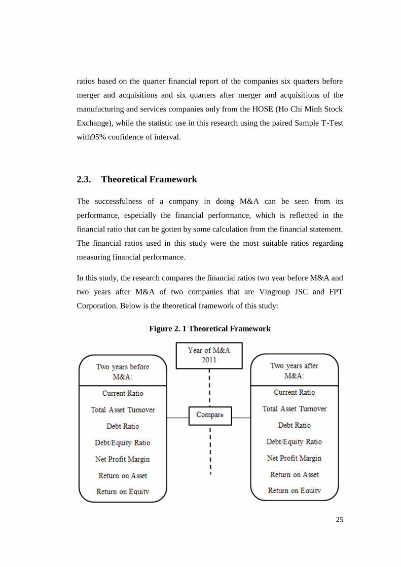
In this study, the research compares the financial ratios two year before M&A and

two years after M&A of two companies that are Vingroup JSC and FPT

Corporation. Below is the theoretical framework of this study:

Figure 2. 1 Theoretical Framework

26

2.4. Operational Definition

2.4.1. Current Ratio:

An indication of a company's ability to meet short-term debt obligations; the

higher the ratio, the more liquid the company is.

2.4.2. Total Asset Turnover Ratio:

This ratio shows how efficiently a company can use its assets to generate sales.

2.4.3. Debt Ratio:

The debt ratio shows a company's ability to pay off its liabilities with its assets. In

other words, this shows how many assets the company must sell in order to pay

off all of its liabilities.

2.4.4. Debt to Equity Ratio:

The debt to equity ratio shows the percentage of company financing that comes

from creditors and investors.

2.4.5. Net Profit Margin:

It shows how good a company is at converting revenue into profits available for

shareholders.

2.4.6. Return on Asset:

It measures how efficiently a company can manage its assets to produce profits

during a period.

2.4.7. Return on Equity:

It shows how much profit each dollar of common stockholders' equity generates.

2.4.8. Earnings per Share:

This is the amount of money each share of stock would receive if all of the profits

were distributed to the outstanding shares at the end of the year.

27

2.5. Hypothesis

Based on the problem statement, there are 8 variables will be tested:

H01: (There is no significant difference between CR before and CR

after M&A)

H02: (There is no significant difference between TATO before and

TATO after M&A)

H03: (There is no significant difference between DR before and DR

after M&A)

H04: (There is no significant difference between DER before and DER

after M&A)

H05: (There is no significant difference NPM before and NPM after

M&A)

H06: (There is no significant difference ROA before and ROA after

M&A)

H07: (There is no significant difference ROE before and ROE after

M&A)

H08: (There is no significant difference EPS before and EPS after

M&A)

28

CHAPTER III

RESEARCH METHODOLOGY

This chapter present the research methods and procedures that are conducted by

the researcher in the process of investigating, sampling design and selection of

respondents, also the procedures in gathering the data and how it is been treated

by statistical application.

3.1. Research Design

There are two methods in doing scientific research those are qualitative and

quantitative research. The differences between qualitative and quantitative

research are the type of data, research process, instrument in collecting data and

the purpose of research.

Qualitative research is type of formative research that includes specialized

techniques for obtaining in-depth responses about what people think and how

they feel. It is seen as the research that seeks answer to the questions in the real

world. Qualitative researchers gather what they see, hear, read from people and

places, from events and activities, with the purpose to learn about the community

and to generate new understanding that can be used by the social world.

Qualitative research has often been conducted to answer the question “why”

rather than “what”. A purpose of qualitative research is the construction of new

understanding. (Amol R Dongre, Pradeep R Deshmukh, Ganapathy Kalaiselvan,

and Sanjeev Upadhyaya., 2009)

Quantitative research is typically considered to be the more “scientific” approach

to doing social science. The focus is on using specific definitions and carefully

operationalizing what particular concepts and variables mean. Qualitative

research methods provide more emphasis on interpretation and providing

29

consumers with complete views, looking at contexts, environmental immersions

and a depth of understanding of concepts. (Tewksbury, 2009)

Quantitative research, on the other hand, is focused on testing the strength and

persistence of relationships between distinct measures. Specifying exactly how

two (or more) very narrow, limited concepts/variables is of value, but often of

value only for very exact measurements of narrowly defined issues, concepts and

variables. As such, quantitative research relies on the ways that researchers

choose to have variables defined, and what they elect to include within the scope

of the definition of variables.

In this research uses quantitative research methodology that has the major

objective to know the company’s financial performance after doing M&A. For

this particular research, quantitative research method is preferred by the

researcher due to its main purpose for measurement.

Researcher chooses quantitative research because quantitative research can

provide specific facts that decision makers can use to (1) make accurate

prediction about the relationship between market factors and behaviors, (2) gain

meaningful insights into those relationships, (3) validate the existing relationship,

and (4) test various types of hypotheses (Joseph F. Hair, Robert P. Bush, and

David J. Ortinau, 2006). In addition, quantitative research uses data that are

structured in the form of numbers or that can be immediately transported into

numbers. It is a very controlled, exact approach to research.

3.2. Sampling Design

The researcher uses the purposive sampling with the criteria: population of

manufacturing and services companies which did M&A in the period 2012 listed

in the HOSE and have the quarters’ financial reports. Sample is the whole

population which includes two companies: Vingroup Joint Stock Company

(Vingroup JSC) and FPT Corporation.

30

1. Vingroup Joint Stock Company (Vingroup JSC), formerly known as

Technocom, was founded in Ukraine in 1993 by an ambitious group of

Vietnamese youths. Technocom began with food production and quickly

found great success with the Mivina brand. During the early years of the

21st century, Technocom was ranked among Ukraine’s Top 100 largest

and most influential companies. In 2000, Technocom - Vingroup returned

to Vietnam with ambition to contribute the country’s development.

Emphasizing sustainable long-term development, Vingroup initially

focused investments on real estate and hospitality through two key brands,

Vincom and Vinpearl.

2. FPT Corporation was founded on September 13rd

, 1988. For almost 26

years of development, FPT has always been the leading ICT Company in

Vietnam with the revenue of more than VND 28,647 billion, equivalent to

nearly USD 1.36 billion, creating more than 17,000 jobs for the society.

The company’s market capitalization (as of Feb 28 2014) reached VND

17,608 billion, being one of the largest private enterprises in Vietnam

(ranked by Vietnam Report 500). FPT conducts the core businesses in the

fields of information technology and telecommunications.

3.3. Research Instrument

In this research, researcher use secondary data as source of data. According to

Guffey and Loewy (2009P), secondary data come from reading what others have

experienced and observed. Secondary data are easier and cheaper to develop than

a primary data, which might involve interviewing large group or sending out

questionnaires. The resources of secondary data are within the firms, business

database services, government agencies, industry associations, special-interest

organizations and internet. The secondary data in this study is collected from the

financial statements which include income statement and balance sheet published

by the companies listed by the companies listed in Vietnamese Stock Exchange

31

and the financial ratio of companies that were provided on VietStock website

official. The researcher also uses some books and journals while completing this

study in order to support the theory, data or information.

The formulas of Financial Ratios are used in this study are explained below:

1. CR: represents the Liquidity Ratios. CR is one of the most common cited

financial ratios, measure the firm’s ability to meet its short-term

obligations.

2. TATO: represents the Activity Ratios. TATO measures a firm’s efficiency

at using its assets in generating sales or revenue – the higher number the

better

3. DR: represents the debt management or leverage ratios. Debt Ratio

measures the proportion of a firm’s total assets that is financed with

creditor’s funds.

4. DER: represent the Debt Management or Leverage Ratios. DER is

computed by dividing total liabilities by equity capital.

32

5. NPM: represents the profitability ratios. NPM is also called Profit Margin

in sales; it is calculated by diving net income by sales. It gives the profit

per dollar of sales.

6. ROA: represents the Profitability Ratios. ROA is an indicator of how

profitable a company is relative to its total assets.

7. ROE: represents profitability Ratios. ROE indicates the accounting rate of

return on the stockholders’ investment, as measured by net income

relative to common equity.

( )

8. EPS: is generally of interest to present or prospective stockholders and

management. EPS represents the number of dollars earned during the

period on behalf of each outstanding share of common stock.

33

3.4. Data Collection Procedure

The data used in this research are financial statement of the Companies to

calculate the Financial Ratio. To be clearer, the data that are used in this research

are stated as follow:

1. Financial Report Quarterly of from 2009 until 2013 for Vingroup JSC.

2. Financial Report Quarterly of from 2009 until 2013 for FPT Corporation.

In conducting this research, the researcher followed this below procedure to

collect the data for the research.

The financial reports of companies are taken from the official website of

Vietstock (http://finance.vietstock.vn/)

3.5. Hypothesis Testing

This part the researcher presents the statistical techniques were used to prove the

hypothesis that was mentioned in Chapter 2. The research will use the T-test and

SPSS 22.0 software for windows.

Figure 3. 1 Research Framework

34

3.5.1. Paired Sample T – Test

A paired sample t-test is used to determine whether there is a significant

difference between the average values of the same measurement made under two

different conditions. Both measurements are made on each unit in a sample, and

the test is based on the paired differences between these two values. The usual

null hypothesis is that the difference in the mean values is zero. (The Statistic

Glossary: Paired Sapmle t-test, 2015)

A pair sample T-test will be undertaken to prove whether there are any

significance differences or not between before and after M&A by comparing the

financial ratios which are Current Ratio, Total Asset Turnover, Debt Ratio, Debt

to Equity Ratio, Net Profit Margin, Return on Asset, Return on Equity , Earning

per Share.

3.5.2. Condition Required for Paired Sample T-Test:

Assumptions:

Assumption 1: Dependent variable should be measured on a continuous scale.

Assumption 2: Independent variable should consist of two categorical, "related

groups" or "matched pairs".

Assumption 3: There should be no significant outliers in the differences between

the two related groups.

Assumption 4: The distribution of the differences in the dependent variable

between the two related groups should be approximately normally distributed.

(statistic laerd: Paired t-test using Minitab, 2015)

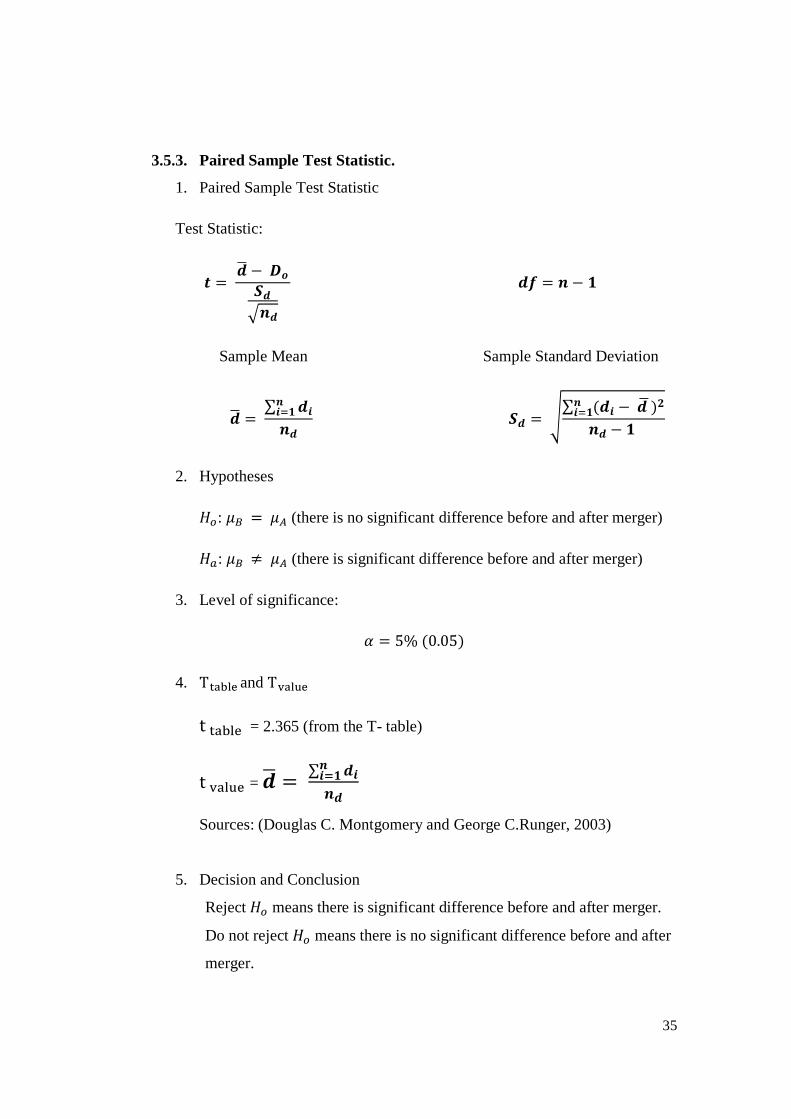
35

3.5.3. Paired Sample Test Statistic.

1. Paired Sample Test Statistic

Test Statistic:

√

Sample Mean Sample Standard Deviation

∑

√

∑ ( )

2. Hypotheses

: (there is no significant difference before and after merger)

: (there is significant difference before and after merger)

3. Level of significance:

( )

4. and

= 2.365 (from the T- table)

= ∑

Sources: (Douglas C. Montgomery and George C.Runger, 2003)

5. Decision and Conclusion

Reject means there is significant difference before and after merger.

Do not reject means there is no significant difference before and after

merger.

36

CHAPTER IV

ANALYSIS AND INTERPRETATION

4.1. Company profile

4.1.1. Vingroup Joint Stock Company (Vingroup JSC)

Vingroup Joint Stock Company (Vingroup JSC), formerly known as Technocom,

was founded in Ukraine in 1993 by an ambitious group of Vietnamese youths.

Technocom began with food production and quickly found great success with the

Mivina brand. During the early years of the 21st century, Technocom was ranked

among Ukraine’s Top 100 largest and most influential companies. In 2000,

Technocom - Vingroup returned to Vietnam with ambition to contribute the

country’s development.

Emphasizing sustainable long-term development, Vingroup initially focused

investments on real estate and hospitality through two key brands, Vincom and

Vinpearl. Ten years of hard work and dedication turned Vincom into one of

Vietnam’s premier real estate brands with a number of mixed-used developments

in major cities, combining modern shopping malls, offices and luxury apartments

in a single complex, leading the trend towards smart, eco-luxury urban projects in

Vietnam. Alongside Vincom and Vinpearl has also become the leader in

Vietnam’s tourism industry, featuring international 5-star and above hotels,

resorts, beach villas, amusement parks and golf courses.

In January 2012, Vinpearl JSC merged into Vincom JSC to form Vingroup JSC.

The new structure ensures sustained development and allows Vingroup to focus

on developing its strategic brands:

1. Vinhomes (Luxury serviced apartments and villas)

2. Vincom (Premium shopping malls)

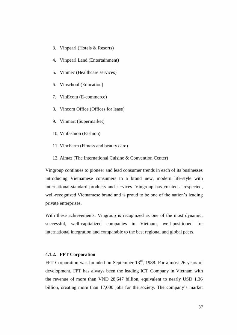
37

3. Vinpearl (Hotels & Resorts)

4. Vinpearl Land (Entertainment)

5. Vinmec (Healthcare services)

6. Vinschool (Education)

7. VinEcom (E-commerce)

8. Vincom Office (Offices for lease)

9. Vinmart (Supermarket)

10. Vinfashion (Fashion)

11. Vincharm (Fitness and beauty care)

12. Almaz (The International Cuisine & Convention Center)

Vingroup continues to pioneer and lead consumer trends in each of its businesses

introducing Vietnamese consumers to a brand new, modern life-style with

international-standard products and services. Vingroup has created a respected,

well-recognized Vietnamese brand and is proud to be one of the nation’s leading

private enterprises.

With these achievements, Vingroup is recognized as one of the most dynamic,

successful, well-capitalized companies in Vietnam, well-positioned for

international integration and comparable to the best regional and global peers.

4.1.2. FPT Corporation

FPT Corporation was founded on September 13rd

, 1988. For almost 26 years of

development, FPT has always been the leading ICT Company in Vietnam with

the revenue of more than VND 28,647 billion, equivalent to nearly USD 1.36

billion, creating more than 17,000 jobs for the society. The company’s market

38

capitalization (as of Feb 28 2014) reached VND 17,608 billion, being one of the

largest private enterprises in Vietnam (ranked by Vietnam Report 500).

FPT conducts the core businesses in the fields of information technology and

telecommunications, FPT has been providing services to fifty seven out of sixty

three cities and provinces of Vietnam and continued expanding its business to the

global market. FPT has had clients or opened representative offices and

companies in 17 countries including Vietnam, Laos, Cambodia, America, Japan,

Singapore, Germany, Myanmar, France, Malaysia, Australia, Thailand, United

Kingdom, Philippines, Kuwait, Bangladesh and Indonesia.

FPT has intensive experience of establishing and implementing large scale

business models. After nearly twenty six years, FPT is now the No. 1 company in

Vietnam specializing in Software Development, System Integration, IT Services,

Distribution and Manufacturing of IT products, and Retails. In

telecommunications area, FPT is one of three biggest Internet services providers

in Vietnam. In regard to content development, FPT is now the No. 1 online

advertising company in Vietnam, owning an e-newspaper with more than 42

million page views per day, which is equal to the number of Internet users in

Vietnam.

4.2. Data Analysis

4.2.1. Overview of the Research Object

Research object used in this research is two companies have implemented in the

period 2011 and are listed on the HOSE (Ho Chi Minh Stock Exchange). From

the criteria given, there are two companies are being researched that are Vingroup

JSC and FPT Corporation.

The financial statements per quarter are used in this research are obtained from

companies’ quarter report, and some ratios were taken from VietStock official

39

website. The other financial ratios are calculated by the researcher based on the

Financial Ratios’ Formula form Principle of Manager Finance Book.

4.2.2. Classical Assumptions:

4.2.2.1. Result of Outliners:

An outlier is an observation that lies an abnormal distance from other values in a

random sample from a population. In a sense, this definition leaves it up to the

analyst (or a consensus process) to decide what will be considered abnormal.

Before abnormal observations can be singled out, it is necessary to characterize

normal observations. (Engineering Statistics Handbook: What are outliners in the

data?, 2015)

The Box plot displays the three quartiles, the minimum, and the maximum of the

data on a rectangular box, aligned either horizontally or vertically. The box

encloses the interquartile range with the left of lower edge at the first quartile and

the right (or lower) edge at the third quartile. A line is drawn through the box at

the second quartile. A line, or whisker, extends from each end of the box. A point

beyond a whisker, but less than 3 interquartile ranges from the box edge, is called

an outliner. (Douglas C. Montgomery and George C.Runger, 2003)

Vingroup JSC:

The difference between before and after merger of CR:

Figure 4. 1 Box Plot for Difference of CR for Vingroup

(Sources: SPSS Data result by SPSS v.22.0)

40

Figure 4. 3 Box Plot for Difference of DR for Vingroup

(Sources: SPSS Data result by SPSS v.22.0)

(Sources: SPSS Data result by SPSS v.22.0)

The figures above show that do not have any point beyond a whisker but less than

3 interquartile ranges from the box edge. It means there is no significant outliner

in the differences between two related group that are CR before and after M&A.

The difference between before and after merger of TATO:

The figures above show that do not have any point beyond a whisker but less than

3 interquartile ranges from the box edge. It means there is no significant outliner

in the differences between two related group that are TATO before and after

M&A.

The difference between before and after merger of DR:

Figure 4. 2 Box Plot for Difference of TATO for Vingroup

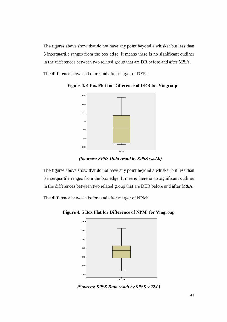
41

(Sources: SPSS Data result by SPSS v.22.0)

(Sources: SPSS Data result by SPSS v.22.0)

The figures above show that do not have any point beyond a whisker but less than

3 interquartile ranges from the box edge. It means there is no significant outliner

in the differences between two related group that are DR before and after M&A.

The difference between before and after merger of DER:

The figures above show that do not have any point beyond a whisker but less than

3 interquartile ranges from the box edge. It means there is no significant outliner

in the differences between two related group that are DER before and after M&A.

The difference between before and after merger of NPM:

Figure 4. 4 Box Plot for Difference of DER for Vingroup

Figure 4. 5 Box Plot for Difference of NPM for Vingroup

42

(Sources: SPSS Data result by SPSS v.22.0)

(Sources: SPSS Data result by SPSS v.22.0)

The figures above show that do not have any point beyond a whisker but less than

3 interquartile ranges from the box edge. It means there is no significant outliner

in the differences between two related group that are NPM before and after M&A.

The difference between before and after merger of ROA:

The figures above show that do not have any point beyond a whisker but less than

3 interquartile ranges from the box edge. It means there is no significant outliner

in the differences between two related group that are ROA before and after M&A.

The difference between before and after merger of ROE:

Figure 4. 6 Box Plot for Difference of ROA for Vingroup

Figure 4. 7 Box Plot for Difference of ROE for Vingroup

43

(Sources: SPSS Data result by SPSS v.22.0)

(Sources: SPSS Data result by SPSS v.22.0)

The figures above show that do not have any point beyond a whisker but less than

3 interquartile ranges from the box edge. It means there is no significant outliner

in the differences between two related group that are ROE before and after M&A.

The difference between before and after merger of EPS:

The figures above show that do not have any point beyond a whisker but less than

3 interquartile ranges from the box edge. It means there is no significant outliner

in the differences between two related group that are EPS before and after M&A.

FPT Corporation:

The difference between before and after merger of CR:

Figure 4. 8 Box Plot for Difference of EPS for Vingroup

Figure 4. 9 Box Plot for Difference of CR for FPT

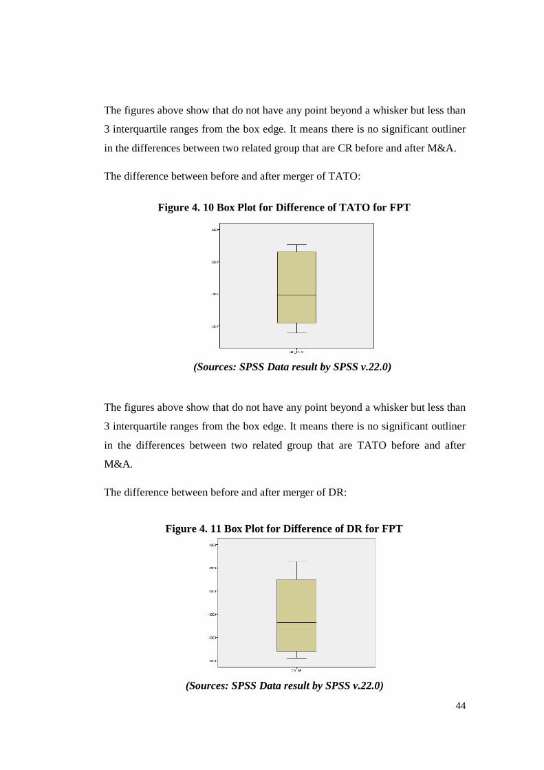
44

(Sources: SPSS Data result by SPSS v.22.0)

(Sources: SPSS Data result by SPSS v.22.0)

The figures above show that do not have any point beyond a whisker but less than

3 interquartile ranges from the box edge. It means there is no significant outliner

in the differences between two related group that are CR before and after M&A.

The difference between before and after merger of TATO:

The figures above show that do not have any point beyond a whisker but less than

3 interquartile ranges from the box edge. It means there is no significant outliner

in the differences between two related group that are TATO before and after

M&A.

The difference between before and after merger of DR:

Figure 4. 10 Box Plot for Difference of TATO for FPT

Figure 4. 11 Box Plot for Difference of DR for FPT

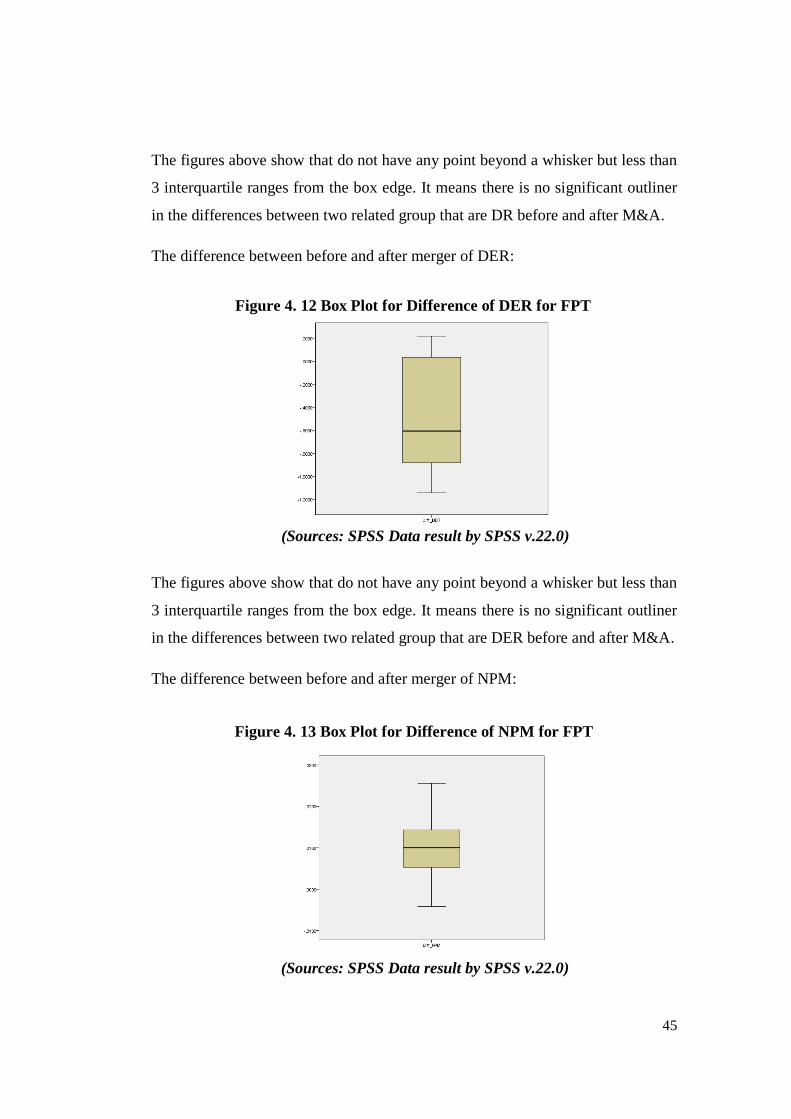
45

Figure 4. 13 Box Plot for Difference of NPM for FPT

(Sources: SPSS Data result by SPSS v.22.0)

(Sources: SPSS Data result by SPSS v.22.0)

The figures above show that do not have any point beyond a whisker but less than

3 interquartile ranges from the box edge. It means there is no significant outliner

in the differences between two related group that are DR before and after M&A.

The difference between before and after merger of DER:

The figures above show that do not have any point beyond a whisker but less than

3 interquartile ranges from the box edge. It means there is no significant outliner

in the differences between two related group that are DER before and after M&A.

The difference between before and after merger of NPM:

Figure 4. 12 Box Plot for Difference of DER for FPT

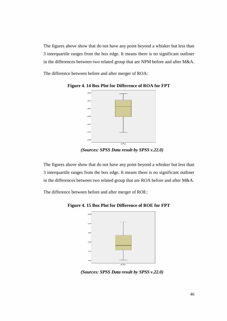
46

(Sources: SPSS Data result by SPSS v.22.0)

(Sources: SPSS Data result by SPSS v.22.0)

The figures above show that do not have any point beyond a whisker but less than

3 interquartile ranges from the box edge. It means there is no significant outliner

in the differences between two related group that are NPM before and after M&A.

The difference between before and after merger of ROA:

The figures above show that do not have any point beyond a whisker but less than

3 interquartile ranges from the box edge. It means there is no significant outliner

in the differences between two related group that are ROA before and after M&A.

The difference between before and after merger of ROE:

Figure 4. 14 Box Plot for Difference of ROA for FPT

Figure 4. 15 Box Plot for Difference of ROE for FPT

47

(Sources: SPSS Data result by SPSS v.22.0)

The figures above show that do not have any point beyond a whisker but less than

3 interquartile ranges from the box edge. It means there is no significant outliner

in the differences between two related group that are ROE before and after M&A.

The difference between before and after merger of EPS:

The figures above show that do not have any point beyond a whisker but less than

3 interquartile ranges from the box edge. It means there is no significant outliner

in the differences between two related group that are CR before and after M&A.

4.2.2.2. Result of the normal distribution test:

The two main tests to test the normal distribution are: Kolmogorov-Smirnoff (K-

S) and Shapiro-Wilks (S-W).

These tests compare the set of scores in a sample to a normally distributed set of

scores with the same mean and standard deviation. If the test is non-significant (ie

p>0.05) then this shows that the data set is not significantly different from a

normal distribution ie the data is normally distributed. If however the test statistic

is significant (ie p <0.05) then the data is not normally distributed. Like all

statistical tests the power of these tests depends on the sample size, and in the test

carried out below SPSS automatically quotes the S-W statistic when the sample

size is less than 100. (Storey, 2014)

Figure 4. 16 Box Plot for Difference of EPS for FPT

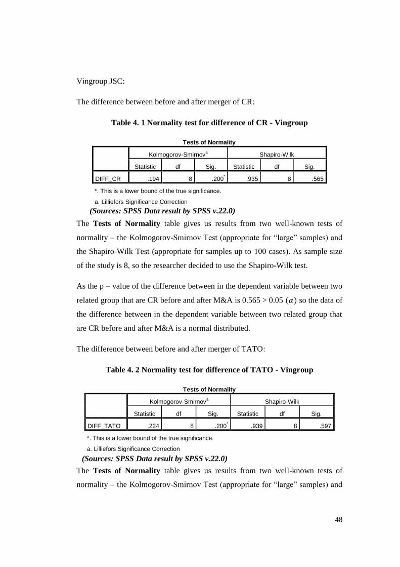
48

(Sources: SPSS Data result by SPSS v.22.0)

(Sources: SPSS Data result by SPSS v.22.0)

Vingroup JSC:

The difference between before and after merger of CR:

Table 4. 1 Normality test for difference of CR - Vingroup

Tests of Normality

Kolmogorov-Smirnova Shapiro-Wilk

Statistic df Sig. Statistic df Sig.

DIFF_CR .194 8 .200* .935 8 .565

*. This is a lower bound of the true significance.

a. Lilliefors Significance Correction

The Tests of Normality table gives us results from two well-known tests of

normality – the Kolmogorov-Smirnov Test (appropriate for “large” samples) and

the Shapiro-Wilk Test (appropriate for samples up to 100 cases). As sample size

of the study is 8, so the researcher decided to use the Shapiro-Wilk test.

As the p – value of the difference between in the dependent variable between two

related group that are CR before and after M&A is 0.565 > 0.05 ( ) so the data of

the difference between in the dependent variable between two related group that

are CR before and after M&A is a normal distributed.

The difference between before and after merger of TATO:

Table 4. 2 Normality test for difference of TATO - Vingroup

Tests of Normality

Kolmogorov-Smirnova Shapiro-Wilk

Statistic df Sig. Statistic df Sig.

DIFF_TATO .224 8 .200* .939 8 .597

*. This is a lower bound of the true significance.

a. Lilliefors Significance Correction

The Tests of Normality table gives us results from two well-known tests of

normality – the Kolmogorov-Smirnov Test (appropriate for “large” samples) and

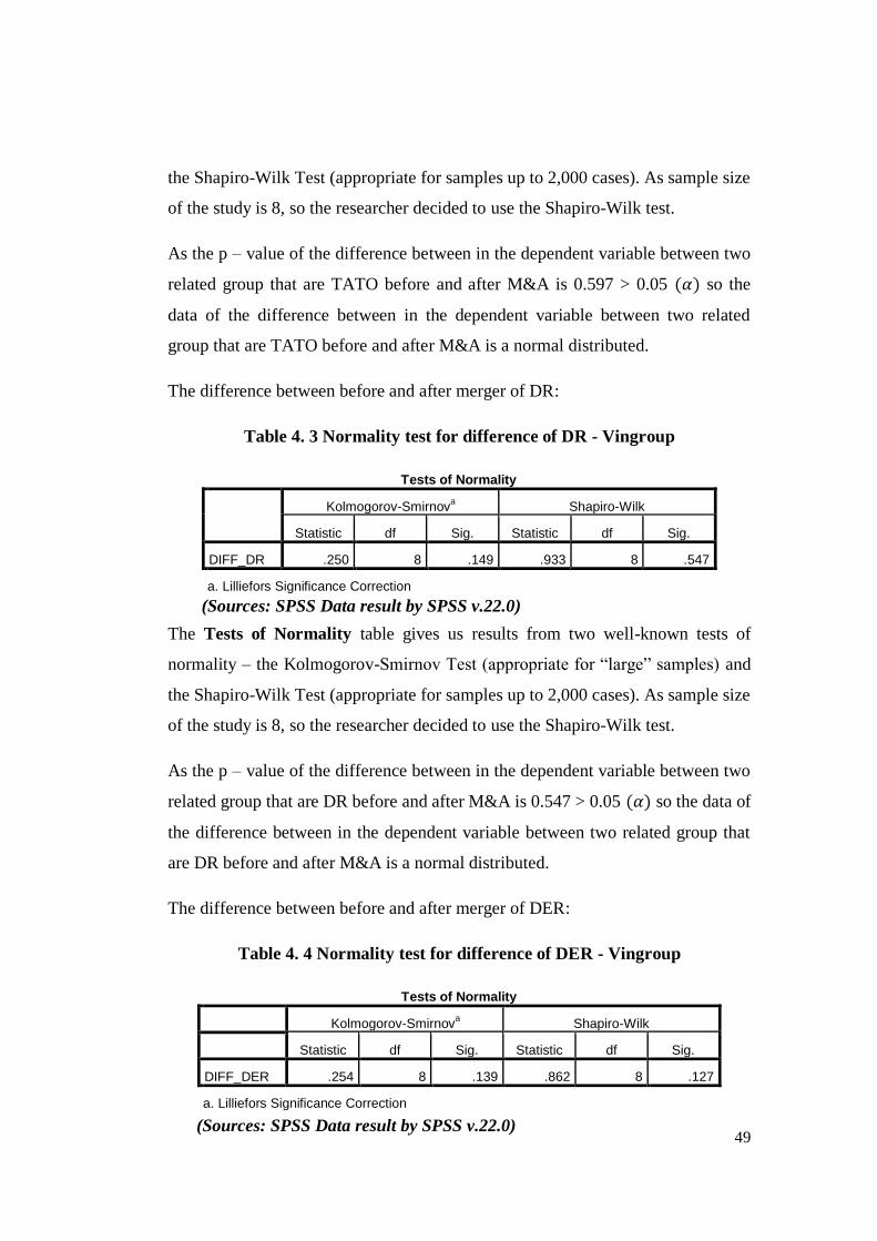
49

(Sources: SPSS Data result by SPSS v.22.0)

(Sources: SPSS Data result by SPSS v.22.0)

the Shapiro-Wilk Test (appropriate for samples up to 2,000 cases). As sample size

of the study is 8, so the researcher decided to use the Shapiro-Wilk test.

As the p – value of the difference between in the dependent variable between two

related group that are TATO before and after M&A is 0.597 > 0.05 ( ) so the

data of the difference between in the dependent variable between two related

group that are TATO before and after M&A is a normal distributed.

The difference between before and after merger of DR:

Table 4. 3 Normality test for difference of DR - Vingroup

Tests of Normality

Kolmogorov-Smirnova Shapiro-Wilk

Statistic df Sig. Statistic df Sig.

DIFF_DR .250 8 .149 .933 8 .547

a. Lilliefors Significance Correction

The Tests of Normality table gives us results from two well-known tests of

normality – the Kolmogorov-Smirnov Test (appropriate for “large” samples) and

the Shapiro-Wilk Test (appropriate for samples up to 2,000 cases). As sample size

of the study is 8, so the researcher decided to use the Shapiro-Wilk test.

As the p – value of the difference between in the dependent variable between two

related group that are DR before and after M&A is 0.547 > 0.05 ( ) so the data of

the difference between in the dependent variable between two related group that

are DR before and after M&A is a normal distributed.

The difference between before and after merger of DER:

Table 4. 4 Normality test for difference of DER - Vingroup

Tests of Normality

Kolmogorov-Smirnova Shapiro-Wilk

Statistic df Sig. Statistic df Sig.

DIFF_DER .254 8 .139 .862 8 .127

a. Lilliefors Significance Correction

50

(Sources: SPSS Data result by SPSS v.22.0)

The Tests of Normality table gives us results from two well-known tests of

normality – the Kolmogorov-Smirnov Test (appropriate for “large” samples) and

the Shapiro-Wilk Test (appropriate for samples up to 2,000 cases). As sample size

of the study is 8, so the researcher decided to use the Shapiro-Wilk test.

As the p – value of the difference between in the dependent variable between two

related group that are DER before and after M&A is 0.127 > 0.05 ( ) so the data

of the difference between in the dependent variable between two related group

that are DER before and after M&A is a normal distributed.

The difference between before and after merger of NPM:

Table 4. 5 Normality test for difference of NPM - Vingroup

Tests of Normality

Kolmogorov-Smirnova Shapiro-Wilk

Statistic df Sig. Statistic df Sig.

DIFF_NPM .178 8 .200* .967 8 .877

*. This is a lower bound of the true significance.

a. Lilliefors Significance Correction

The Tests of Normality table gives us results from two well-known tests of

normality – the Kolmogorov-Smirnov Test (appropriate for “large” samples) and

the Shapiro-Wilk Test (appropriate for samples up to 2,000 cases). As sample size

of the study is 8, so the researcher decided to use the Shapiro-Wilk test.

As the p – value of the difference between in the dependent variable between two

related group that are NPM before and after M&A is 0.877 > 0.05 ( ) so the data

of the difference between in the dependent variable between two related group

that are NPM before and after M&A is a normal distributed.

51

(Sources: SPSS Data result by SPSS v.22.0)

(Sources: SPSS Data result by SPSS v.22.0)

The difference between before and after merger of ROA:

Table 4. 6 Normality test for difference of ROA - Vingroup

Tests of Normality

Kolmogorov-Smirnova Shapiro-Wilk

Statistic df Sig. Statistic df Sig.

DIFF_ROA .167 8 .200* .975 8 .932

*. This is a lower bound of the true significance.

a. Lilliefors Significance Correction

The Tests of Normality table gives us results from two well-known tests of

normality – the Kolmogorov-Smirnov Test (appropriate for “large” samples) and

the Shapiro-Wilk Test (appropriate for samples up to 2,000 cases). As sample size

of the study is 8, so the researcher decided to use the Shapiro-Wilk test.

As the p – value of the difference between in the dependent variable between two

related group that are ROA before and after M&A is 0.932 > 0.05 ( ) so the data

of the difference between in the dependent variable between two related group

that are ROA before and after M&A is a normal distributed.

The difference between before and after merger of ROE:

Table 4. 7 Normality test for difference of ROE - Vingroup

Tests of Normality

Kolmogorov-Smirnova Shapiro-Wilk

Statistic df Sig. Statistic df Sig.

DIFF_ROE .218 8 .200* .906 8 .328

*. This is a lower bound of the true significance.

a. Lilliefors Significance Correction

The Tests of Normality table gives us results from two well-known tests of

normality – the Kolmogorov-Smirnov Test (appropriate for “large” samples) and

the Shapiro-Wilk Test (appropriate for samples up to 2,000 cases). As sample size

of the study is 8, so the researcher decided to use the Shapiro-Wilk test.

52

(Sources: SPSS Data result by SPSS v.22.0)

(Sources: SPSS Data result by SPSS v.22.0)

As the p – value of the difference between in the dependent variable between two

related group that are ROE before and after M&A is 0.328 > 0.05 ( ) so the data

of the difference between in the dependent variable between two related group

that are ROE before and after M&A is a normal distributed.

The difference between before and after merger of EPS:

Table 4. 8 Normality test for difference of EPS - Vingroup

Tests of Normality

Kolmogorov-Smirnova Shapiro-Wilk

Statistic df Sig. Statistic df Sig.

DIFF_EPS .214 8 .200* .952 8 .733

*. This is a lower bound of the true significance.

a. Lilliefors Significance Correction

The Tests of Normality table gives us results from two well-known tests of

normality – the Kolmogorov-Smirnov Test (appropriate for “large” samples) and

the Shapiro-Wilk Test (appropriate for samples up to 2,000 cases). As sample size

of the study is 8, so the researcher decided to use the Shapiro-Wilk test.

As the p – value of the difference between in the dependent variable between two

related group that are EPS before and after M&A is 0.733 > 0.05 ( ) so the data

of the difference between in the dependent variable between two related group

that are EPS before and after M&A is a normal distributed.

FPT Corporation:

The difference between before and after merger of CR:

Table 4. 9 Normality test for difference of CR - FPT

Tests of Normality

Kolmogorov-Smirnova Shapiro-Wilk

Statistic df Sig. Statistic df Sig.

Diff_CR .243 8 .180 .906 8 .329

a. Lilliefors Significance Correction

53

(Sources: SPSS Data result by SPSS v.22.0)

The Tests of Normality table gives us results from two well-known tests of

normality – the Kolmogorov-Smirnov Test (appropriate for “large” samples) and

the Shapiro-Wilk Test (appropriate for samples up to 2,000 cases). As sample size

of the study is 8, so the researcher decided to use the Shapiro-Wilk test.

As the p – value of the difference between in the dependent variable between two

related group that are CR before and after M&A is 0.329 > 0.05 ( ) so the data of

the difference between in the dependent variable between two related group that

are CR before and after M&A is a normal distributed.

The difference between before and after merger of TATO:

Table 4. 10 Normality test for difference of TATO - FPT

Tests of Normality

Kolmogorov-Smirnova Shapiro-Wilk

Statistic df Sig. Statistic df Sig.

Diff_TATO .179 8 .200* .887 8 .222

*. This is a lower bound of the true significance.

a. Lilliefors Significance Correction

The Tests of Normality table gives us results from two well-known tests of

normality – the Kolmogorov-Smirnov Test (appropriate for “large” samples) and

the Shapiro-Wilk Test (appropriate for samples up to 2,000 cases). As sample size

of the study is 8, so the researcher decided to use the Shapiro-Wilk test.

As the p – value of the difference between in the dependent variable between two

related group that are TATO before and after M&A is 0.222> 0.05 ( ) so the data

of the difference between in the dependent variable between two related group

that are TATO before and after M&A is a normal distributed.

54

(Sources: SPSS Data result by SPSS v.22.0)

(Sources: SPSS Data result by SPSS v.22.0)

The difference between before and after merger of DR:

Table 4. 11 Normality test for difference of DR - FPT

Tests of Normality

Kolmogorov-Smirnova Shapiro-Wilk

Statistic df Sig. Statistic df Sig.

Diff_DR .189 8 .200* .900 8 .288

*. This is a lower bound of the true significance.

a. Lilliefors Significance Correction

The Tests of Normality table gives us results from two well-known tests of

normality – the Kolmogorov-Smirnov Test (appropriate for “large” samples) and

the Shapiro-Wilk Test (appropriate for samples up to 2,000 cases). As sample size

of the study is 8, so the researcher decided to use the Shapiro-Wilk test.

As the p – value of the difference between in the dependent variable between two

related group that are DR before and after M&A is 0.288> 0.05 ( ) so the data of

the difference between in the dependent variable between two related group that

are DR before and after M&A is a normal distributed.

The difference between before and after merger of DER:

Table 4. 12 Normality test for difference of DER - FPT

Tests of Normality

Kolmogorov-Smirnova Shapiro-Wilk

Statistic df Sig. Statistic df Sig.

Diff_DER .205 8 .200* .912 8 .368

*. This is a lower bound of the true significance.

a. Lilliefors Significance Correction

The Tests of Normality table gives us results from two well-known tests of

normality – the Kolmogorov-Smirnov Test (appropriate for “large” samples) and

the Shapiro-Wilk Test (appropriate for samples up to 2,000 cases). As sample size

of the study is 8, so the researcher decided to use the Shapiro-Wilk test.

55

(Sources: SPSS Data result by SPSS v.22.0)

(Sources: SPSS Data result by SPSS v.22.0)

As the p – value of the difference between in the dependent variable between two

related group that are DER before and after M&A is 0.368 > 0.05 ( ) so the data

of the difference between in the dependent variable between two related group

that are DER before and after M&A is a normal distributed.

The difference between before and after merger of NPM:

Table 4. 13 Normality test for difference of NPM - FPT

Tests of Normality

Kolmogorov-Smirnova Shapiro-Wilk

Statistic df Sig. Statistic df Sig.

Diff_NPM .164 8 .200* .975 8 .934

*. This is a lower bound of the true significance.

a. Lilliefors Significance Correction

The Tests of Normality table gives us results from two well-known tests of

normality – the Kolmogorov-Smirnov Test (appropriate for “large” samples) and

the Shapiro-Wilk Test (appropriate for samples up to 2,000 cases). As sample size

of the study is 8, so the researcher decided to use the Shapiro-Wilk test.

As the p – value of the difference between in the dependent variable between two

related group that are NPM before and after M&A is 0.934 > 0.05 ( ) so the data

of the difference between in the dependent variable between two related group

that are NPM before and after M&A is a normal distributed.

The difference between before and after merger of ROA:

Table 4. 14 Normality test for difference of ROA - FPT

Tests of Normality

Kolmogorov-Smirnova Shapiro-Wilk

Statistic df Sig. Statistic df Sig.

Diff_ROA .147 8 .200* .949 8 .703

*. This is a lower bound of the true significance.

a. Lilliefors Significance Correction

56

(Sources: SPSS Data result by SPSS v.22.0)

The Tests of Normality table gives us results from two well-known tests of

normality – the Kolmogorov-Smirnov Test (appropriate for “large” samples) and

the Shapiro-Wilk Test (appropriate for samples up to 2,000 cases). As sample size

of the study is 8, so the researcher decided to use the Shapiro-Wilk test.

As the p – value of the difference between in the dependent variable between two

related group that are ROA before and after M&A is 0.703 > 0.05 ( ) so the data

of the difference between in the dependent variable between two related group

that are ROA before and after M&A is a normal distributed.

The difference between before and after merger of ROE:

Table 4. 15 Normality test for difference of ROE - FPT

Tests of Normality

Kolmogorov-Smirnova Shapiro-Wilk

Statistic df Sig. Statistic df Sig.

Diff_ROE .198 8 .200* .970 8 .902

*. This is a lower bound of the true significance.

a. Lilliefors Significance Correction

The Tests of Normality table gives us results from two well-known tests of

normality – the Kolmogorov-Smirnov Test (appropriate for “large” samples) and

the Shapiro-Wilk Test (appropriate for samples up to 2,000 cases). As sample size

of the study is 8, so the researcher decided to use the Shapiro-Wilk test.

As the p – value of the difference between in the dependent variable between two

related group that are ROE before and after M&A is 0.902 > 0.05 ( ) so the data

of the difference between in the dependent variable between two related group

that are ROE before and after M&A is a normal distributed.

57

(Sources: SPSS Data result by SPSS v.22.0)

The difference between before and after merger of EPS:

Table 4. 16 Normality test for difference of EPS - FPT

Tests of Normality

Kolmogorov-Smirnova Shapiro-Wilk

Statistic df Sig. Statistic df Sig.

Diff_EPS .194 8 .200* .963 8 .838

*. This is a lower bound of the true significance.

a. Lilliefors Significance Correction

The Tests of Normality table gives us results from two well-known tests of

normality – the Kolmogorov-Smirnov Test (appropriate for “large” samples) and

the Shapiro-Wilk Test (appropriate for samples up to 2,000 cases). As sample size

of the study is 8, so the researcher decided to use the Shapiro-Wilk test.

As the p – value of the difference between in the dependent variable between two

related group that are EPS before and after M&A is 0.838 > 0.05 ( ) so the data

of the difference between in the dependent variable between two related group

that are EPS before and after M&A is a normal distributed.

4.3. Result of the paired sample test statistics:

The outcome of any hypothesis test you do is the P-value. SPSS isn’t always

consistent in what it calls the P-value, but Sig is always included somewhere. The

P-value measures the strength of evidence against the null hypothesis, H0. The

smaller the P-value, the stronger the evidence against H0.

A test result is significant when the P-value is “small enough”; usually we opt for

any P-values less than 0.05 (5%). (Marion Blumenstein and Leila Boyle, 2014)

Vingroup JSC:

CR variables:

58

(Sources: SPSS Data result by SPSS v.22.0)

(Sources: SPSS Data result by SPSS v.22.0)

Table 4. 17 Paired Samples Test for CR of Vingroup

Paired Samples Test

Paired Differences

t

d

f

Sig.

(2-

tailed

) Mean

Std.

Deviation

Std.

Error

Mean

95% Confidence

Interval of the

Difference

Lower Upper

Pai

r 1

CRBEFOR

E -

CRAFTER

2.987437

5

1.415641

2

.500504

7

1.803931

8

4.170943

2

5.96

9 7 .001

From the table above and according to the statistic calculation for the 95%

confidence interval and two-tailed test, which has a T-table is 2.365, could be

concluded that there is significant difference of CR, whereby the T-value and the

significant were not in the accepted range of H01 with Sig. (two-tailed) 0.01 <

0.05, which means H01 is rejected and Ha 1 is accepted.

TATO variables:

Table 4. 18 Paired Samples Test for TATO of Vingroup

Paired Samples Test

Paired Differences

t df

Sig.

(2-

tailed) Mean

Std.

Deviation

Std. Error

Mean

95% Confidence

Interval of the

Difference

Lower Upper

Pair

1

TATOBEFORE

– TATOAFTER

-

.0166750 .0559524 .0197822

-

.0634524 .0301024

-

.843 7 .427

From the table above and according to the statistic calculation for the 95%

confidence interval and two-tailed test, which has a T-table is 2.365, could be

concluded that there is no significant difference of TATO, whereby the T-value

and the significant were in the accepted range of H02 with Sig. (two-tailed) 0.427

> 0.05, which means do not reject H02 .

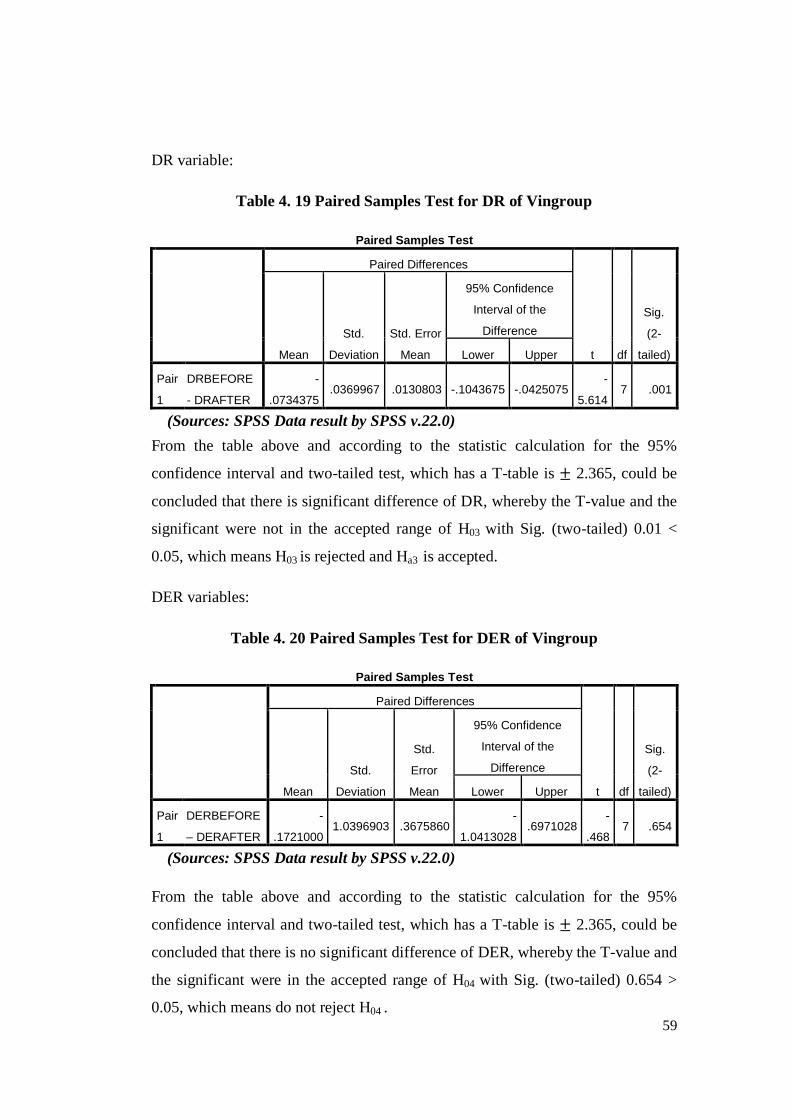
59

(Sources: SPSS Data result by SPSS v.22.0)

(Sources: SPSS Data result by SPSS v.22.0)

DR variable:

Table 4. 19 Paired Samples Test for DR of Vingroup

Paired Samples Test

Paired Differences

t df

Sig.

(2-

tailed) Mean

Std.

Deviation

Std. Error

Mean

95% Confidence

Interval of the

Difference

Lower Upper

Pair

1

DRBEFORE

- DRAFTER

-

.0734375 .0369967 .0130803 -.1043675 -.0425075

-

5.614 7 .001

From the table above and according to the statistic calculation for the 95%

confidence interval and two-tailed test, which has a T-table is 2.365, could be

concluded that there is significant difference of DR, whereby the T-value and the

significant were not in the accepted range of H03 with Sig. (two-tailed) 0.01 <

0.05, which means H03 is rejected and Ha3 is accepted.

DER variables:

Table 4. 20 Paired Samples Test for DER of Vingroup

Paired Samples Test

Paired Differences

t df

Sig.

(2-

tailed) Mean

Std.

Deviation

Std.

Error

Mean

95% Confidence

Interval of the

Difference

Lower Upper

Pair

1

DERBEFORE

– DERAFTER

-

.1721000 1.0396903 .3675860

-

1.0413028 .6971028

-

.468 7 .654

From the table above and according to the statistic calculation for the 95%

confidence interval and two-tailed test, which has a T-table is 2.365, could be

concluded that there is no significant difference of DER, whereby the T-value and

the significant were in the accepted range of H04 with Sig. (two-tailed) 0.654 >

0.05, which means do not reject H04 .

60

(Sources: SPSS Data result by SPSS v.22.0)

(Sources: SPSS Data result by SPSS v.22.0)

NPM variables:

Table 4. 21 Paired Samples Test for NPM of Vingroup

Paired Samples Test

Paired Differences

t df

Sig.

(2-

tailed) Mean

Std.

Deviation

Std. Error

Mean

95% Confidence

Interval of the

Difference

Lower Upper

Pair

1

NPMBEFORE

- NPMAFTER .1611375 .7186397 .2540775

-

.4396603 .7619353 .634 7 .546

From the table above and according to the statistic calculation for the 95%

confidence interval and two-tailed test, which has a T-table is 2.365, could be

concluded that there is no significant difference of NPM, whereby the T-value

and the significant were in the accepted range of H05 with Sig. (two-tailed) 0.546>

0.05, which means do not reject H05 .

ROA variables:

Table 4. 22 Paired Samples Test for ROA of Vingroup

Paired Samples Test

Paired Differences

t df

Sig.

(2-

tailed) Mean

Std.

Deviation

Std. Error

Mean

95% Confidence

Interval of the

Difference

Lower Upper

Pair

1

ROABEFORE

- ROAAFTER .0015000 .0393768 .0139218

-

.0314198 .0344198 .108 7 .917

From the table above and according to the statistic calculation for the 95%

confidence interval and two-tailed test, which has a T-table is 2.365, could be

concluded that there is no significant difference of ROA, whereby the T-value

and the significant were in the accepted range of H06 with Sig. (two-tailed) 0.917

> 0.05, which means do not reject H06 .

61

(Sources: SPSS Data result by SPSS v.22.0)

(Sources: SPSS Data result by SPSS v.22.0)

ROE variables:

Table 4. 23 Paired Samples Test for ROE of Vingroup

Paired Samples Test

Paired Differences

t df

Sig.

(2-

tailed) Mean

Std.

Deviation

Std. Error

Mean

95% Confidence

Interval of the

Difference

Lower Upper

Pair

1

ROEBEFORE

- ROEAFTER .0166375 .1727950 .0610923

-

.1278227 .1610977 .272 7 .793

From the table above and according to the statistic calculation for the 95%

confidence interval and two-tailed test, which has a T-table is 2.365, could be

concluded that there is no significant difference of ROE, whereby the T-value and

the significant were in the accepted range of H07 with Sig. (two-tailed) 0.793 >

0.05, which means do not reject H07 .

EPS variables:

Table 4. 24 Paired Samples Test for EPS of Vingroup

Paired Samples Test

Paired Differences

t df

Sig.

(2-

tailed) Mean

Std.

Deviation

Std. Error

Mean

95% Confidence

Interval of the

Difference

Lower Upper

Pair

1

EPSBEFORE

- EPSAFTER 158.625 2969.473 1049.867 -2323.917 2641.167 .151 7 .884

From the table above and according to the statistic calculation for the 95%

confidence interval and two-tailed test, which has a T-table is 2.365, could be

concluded that there is no significant difference of EPS, whereby the T-value and

the significant were in the accepted range of H08 with Sig. (two-tailed) 0.884 >

0.05, which means do not reject H08 .

62

(Sources: SPSS Data result by SPSS v.22.0)

(Sources: SPSS Data result by SPSS v.22.0)

FPT Corporation:

CR variables:

Table 4. 25 Paired Samples Test for CR of FPT

Paired Samples Test

Paired Differences

t df

Sig.

(2-

tailed) Mean

Std.

Deviation

Std. Error

Mean

95% Confidence

Interval of the

Difference

Lower Upper

Pair

1

CRBEFORE

- CRAFTER .1478000 .0693558 .0245210 .0898171 .2057829 6.027 7 .001

From the table above and according to the statistic calculation for the 95%

confidence interval and two-tailed test, which has a T-table is 2.365, could be

concluded that there is significant difference of CR, whereby the T-value and the

significant were not in the accepted range of H03 with Sig. (two-tailed) 0.01 <

0.05, which means H01 is rejected and Ha1 is accepted.

TATO variables:

Table 4. 26 Paired Samples Test for TATO of FPT

Paired Samples Test

Paired Differences

t df

Sig.

(2-

tailed) Mean

Std.

Deviation

Std.

Error

Mean

95% Confidence

Interval of the

Difference

Lower Upper

Pair

1

TATOBEFORE

- TATOAFTER .4257750 .2278342 .0805516 .2353008 .6162492 5.286 7 .001

From the table above and according to the statistic calculation for the 95%

confidence interval and two-tailed test, which has a T-table is 2.365, could be

concluded that there is significant difference of TATO, whereby the T-value and

63

(Sources: SPSS Data result by SPSS v.22.0)

(Sources: SPSS Data result by SPSS v.22.0)

the significant were not in the accepted range of H03 with Sig. (two-tailed) 0.01 <

0.05, which means H02 is rejected and Ha 2 is accepted.

DR variable:

Table 4. 27 Paired Samples Test for DR of FPT

Paired Samples Test

Paired Differences

t df

Sig.

(2-

tailed) Mean

Std.

Deviation

Std. Error

Mean

95% Confidence

Interval of the

Difference

Lower Upper

Pair

1

DRBEFORE

- DRAFTER .0532125 .0817450 .0289012 -.0151280 .1215530 1.841 7 .108

From the table above and according to the statistic calculation for the 95%

confidence interval and two-tailed test, which has a T-table is 2.365, could be

concluded that there is no significant difference of DR, whereby the T-value and

the significant were in the accepted range of H03 with Sig. (two-tailed) 0.108 >

0.05, which means do not reject H03 .

DER variables:

Table 4. 28 Paired Samples Test for DER of FPT

Paired Samples Test

Paired Differences

t df

Sig.

(2-

tailed) Mean

Std.

Deviation

Std. Error

Mean

95% Confidence

Interval of the

Difference

Lower Upper

Pair

1

DERBEFORE

- DERAFTER .4796375 .5099340 .1802889 .0533220 .9059530 2.660 7 .032

From the table above and according to the statistic calculation for the 95%

confidence interval and two-tailed test, which has a T-table is 2.365, could be

concluded that there is significant difference of DER, whereby the T-value and

64

(Sources: SPSS Data result by SPSS v.22.0)

the significant were not in the accepted range of H04 with Sig. (two-tailed) 0.032 <

0.05, which means H04 is rejected and Ha 4 is accepted.

NPM variables:

Table 4. 29 Paired Samples Test for NPM of FPT

Paired Samples Test

Paired Differences

t df

Sig.

(2-

tailed) Mean

Std.

Deviation

Std. Error

Mean

95% Confidence

Interval of the

Difference

Lower Upper

Pair

1

NPMBEFORE

- NPMAFTER

-

.0100750 .0087739 .0031021

-

.0174102

-

.0027398

-

3.248 7 .014

From the table above and according to the statistic calculation for the 95%

confidence interval and two-tailed test, which has a T-table is 2.365, could be

concluded that there is significant difference of NPM, whereby the T-value and

the significant were not in the accepted range of H05 with Sig. (two-tailed) 0.014 <

0.05, which means H05 is rejected and Ha 5 is accepted.

65

(Sources: SPSS Data result by SPSS v.22.0)

(Sources: SPSS Data result by SPSS v.22.0)

ROA variables:

Table 4. 30 Paired Samples Test for ROA of FPT

Paired Samples Test

Paired Differences

t df

Sig.

(2-

tailed) Mean

Std.

Deviation

Std. Error

Mean

95% Confidence

Interval of the

Difference

Lower Upper

Pair

1

ROABEFORE

- ROAAFTER .0053750 .0081250 .0028726

-

.0014177 .0121677 1.871 7 .104

From the table above and according to the statistic calculation for the 95%

confidence interval and two-tailed test, which has a T-table is 2.365, could be

concluded that there is no significant difference of ROA, whereby the T-value

and the significant were in the accepted range of H06 with Sig. (two-tailed) 0.104

> 0.05, which means do not reject H06 .

ROE variables:

Table 4. 31 Paired Samples Test for ROE of FPT

Paired Samples Test

Paired Differences

t df

Sig.

(2-

tailed) Mean

Std.

Deviation

Std. Error

Mean

95% Confidence

Interval of the

Difference

Lower Upper

Pair

1

ROEBEFORE

- ROEAFTER .0289750 .0129039 .0045622 .0181871 .0397629 6.351 7 .000

From the table above and according to the statistic calculation for the 95%

confidence interval and two-tailed test, which has a T-table is 2.365, could be

concluded that there is significant difference of ROE, whereby the T-value and

the significant were not in the accepted range of H07 with Sig. (two-tailed) 0.000 <

0.05, which means H07 is rejected and Ha 7 is accepted.

66

(Sources: SPSS Data result by SPSS v.22.0)

EPS variables:

Table 4. 32 Paired Samples Test for EPS of FPT

Paired Samples Test

Paired Differences

t df

Sig.

(2-

tailed) Mean

Std.

Deviation

Std.

Error

Mean

95% Confidence

Interval of the

Difference

Lower Upper

Pair

1

EPSBEFORE -

EPSAFTER 379.500 376.687 133.179 64.581 694.419 2.850 7 .025

From the table above and according to the statistic calculation for the 95%

confidence interval and two-tailed test, which has a T-table is 2.365, could be

concluded that there is significant difference of EPS, whereby the T-value and the

significant were not in the accepted range of H05 with Sig. (two-tailed) 0.025 <

0.05, which means H08 is rejected and Ha8 is accepted.

4.4. Interpretation Analysis:

4.4.1.1. The financial performance of Vingroup Company before and

after M&A:

The result of this thesis showed that the financial performance of the company did

not have a lot differences before and after M&A as proved by the Paired Sample

T-Test with six ratios out of eight ratios that the researcher has chosen have no

significance difference before and after M&A. Those ratios are TATO, DER,

NPM, ROA, ROE, and EPS. But the M&A still has effect to the company’s

financial performance that is showed through two ratios that have significance

difference before and after M&A that are CR and DR.

67

So, in Vingroup Company after the M&A, the M&A did not have a lot of

influences to the company performance in Profitability and Activities but it

influences to the Leverage and Liquidity Ratios of the Company.

4.4.1.2. The financial performance of FPT Corporation before and after

M&A:

The result of this thesis showed that the financial performance of the company did

have a lot differences before and after M&A as proved by the Paired Sample T-

Test with only two ratios out of eight ratios that the researcher has chosen have no

significance difference before and after M&A. Those ratios are DR and ROA.

The rest of the ratios those are six ratios that have significance difference before

and after M&A that are CR, TATO, DER, NPM, ROE, and EPS.

68

CHAPTER V

CONCLUSION AND RECOMMENDATION

5.1. Conclusion

The purpose of this research is to analyze the companies’ performance before and

after M&A to find out the effect of M&A to the companies’ performance.

According to the analysis and the elaboration of the impact of merger on

performance of two companies that are: Vingroup JSC and FPT Corporation in

Chapter IV, hence it can be summarized as follow:

For Vingroup JSC:

There has no significant difference before and after M&A on TATO. So it means

that the M&A did not influence to the TATO of the company or can say that the

M&A did not affect the firm's management uses its assets to generate sales.

There has no significant difference before and after M&A on DER. So it means

that the M&A did not influence to the DER of the company or can say that the

M&A did not affect the percentage of the company financing that comes from

creditors and investors.

There has no significant difference before and after M&A on NPM. So it means

that the M&A did not influence to the NPM of the company or can say that the

M&A did not affect how the company converts revenue into profits available for

shareholders.

There has no significant difference before and after M&A on ROA. So it means

that the M&A did not influence to the ROA of the company or can say that the

M&A did not affect how efficiently the company manages its assets to produce

profits.

69

There has no significant difference before and after M&A on ROE. So it means

that the M&A did not influence to the ROE of the company or can say that the

M&A did not affect how much profit each dollar of the common stockholders’

equity generates.

There has no significant difference before and after M&A on EPS. So it means

that the M&A did not influence to the EPS of the company, or can say that the

M&A did not affect the amount of money each share of stock would receive.

There has significant difference before and after M&A on CR. So it means that

the M&A did not influence to the CR of the company or can say that the M&A

did affect the ability of the company to full fill the short term obligation.

There has significant difference before and after M&A on DR. So it means that

the M&A did not influence to the DR of the company or can say that the M&A

did affect the leverage of the company.

For Vingroup JSC, there are six financial ratios which are TATO, DER, NPM,

ROA, ROE, and EPS has no significant difference before and after M&A and

have two ratios that are CR and DR has a significant difference before and after

M&A. So it can be concluded that the financial performance of Vingroup JSC

have changed after M&A but it is not significant difference, it means that there is

no significant different of the financial performance of the company before and

after M&A.

FPT Corporation

There has significant difference before and after M&A on CR. So it means that

the M&A did not influence to the CR of the company or can say that the M&A

did affect the ability of the company to full fill the short term obligation.

There has significant difference before and after M&A on TATO. So it means

that the M&A did not influence to the TATO of the company or can say that the

M&A did affect the firm's management uses its assets to generate sales.

70

There has significant difference before and after M&A on DER. So it means that

the M&A did not influence to the DER of the company or can say that the M&A

did affect the percentage of the company financing that comes from creditors and

investors.

There has significant difference before and after M&A on NPM. So it means that

the M&A did not influence to the NPM of the company or can say that the M&A

did affect how the company converts revenue into profits available for

shareholders.

There has significant difference before and after M&A on ROE. So it means that

the M&A did not influence to the ROE of the company or can say that the M&A

did affect how much profit each dollar of the common stockholders’ equity

generates.

There has significant difference before and after M&A on EPS. So it means that

the M&A did not influence to the EPS of the company or can say that the M&A

did affect the amount of money each share of stock would receive.

There has no significant difference before and after M&A on DR. So it means

that the M&A did not influence to the DR of the company or can say that the

M&A did not affect the leverage of the company.

There has no significant difference before and after M&A on ROA. So it means

that the M&A did not influence to the ROA of the company or can say that the

M&A did not affect how efficiently the company manages its assets to produce

profits.

For the FPT Corporation, there are six ratios which are CR, TATO, DER, NPM,

ROE and EPS that showed a significant difference, but the other two ratios have

no significant differences after M&A that are DR and ROA. So it could be

concluded that the financial performance of the FPT Corporation before and after

M&A has changed or can say that the M&A had effect to the company’s

performance. However, it could not be concluded completely that the reasons of

71

those changes are from M&A. Because besides M&A is the factor can affect to

the company’s financial performance there are still having a lot of the Economy’s

factors that influence the company’s financial performance mostly.

The result is some companies can be influenced by M&A and some company

does not be influenced by M&A. For the companies were influenced by M&A, it

could not be concluded that M&A is only reason of those changes of the

companies’ performance.

The result of this research might have not indicated any significance impacts of

M&A cases of two represented companies. However, it does not mean that this is

the final outcome. It is expected that the M&A will bring a good impact and

challenges to the companies in an appropriate time period and the companies can

avoid the failure of M&A and exploit the benefit of M&A. It was presumed that

to reach the synergy of the M&A is needed more than two years analyzing for

companies were not affected by M&A.

Even though, two years before and two years after is not enough, it is expected

that the time period needed to reach the synergy will not be too long. Since, the

main objective of M&A is to create the synergy between them, hopefully it will

be reached in tan appropriate of time period and hence it can minimize the

operating costs and provide the better services and products to the customer in

order to enhance the position in the market.

5.2. Recommendation

After this study, the researcher would like to give some recommendations

regarding to this research:

1. For companies:

For the companies that have plan to M&A or implement M&A, there are some

recommendations from the researcher:

72

Consider the Debt that the companies might take after the M&A. Because it will

increases the Leverage Business and Finance for the companies in the future. This

will make the companies have heavier burdens that need to solve.

And the companies should pay the attention to the intangible assets of the target

company that are the brand, the patent, the copyright and goodwill, because in the

future the value of them will increase. Besides those aspects, the companies

should consider about the economy and policy that will make a lot of effect to the

financial performance of companies.

2. For the investor:

The investor should be aware of the challenges of M&A. So investor can prepare

the solution to face the problems.

3. For the future researcher:

For who would like to choose M&A as the topic of the research:

1. It will be better if the research include the other factors from the

economy rather than comparing only the Financial Ratios.

2. The time length of the analyzing should be longer so it can show the clear

effect of M&A toward the companies’ performance. Because, M&A has

a long term effect.

73

REFERENCES

Books:

Colman, Helene Loe, Stensaker, Inger og Tharaldsen, Jorunn Elise . (2011).

Activities. Fagbokforlaget.

Dash, A. (2010). Mergers and Acquisitions. New Delhi: I.K. International

Publishing House Pvt. Ltd.

Dash, A. P. (2010). Mergers And Acquisitions. New Delhi: I. K. International Pvt

Ltd.

Douglas C. Montgomery and George C.Runger. (2003). Applied Statistics and

robability for Engineers. New York : John Wiley & Sons, Inc.

Esteban C. Buljevich,Yoon S. Park. (1999). Project Financing and the

International Financial Markets. Massachusetts: Kluwer Academic

Publishers Group .

Gaughan, P. A. (2011). Mergers, Acquisitions and corporate restructuring (Fifth

Edition ed.). New Jersey: John Wiley & Sons.

Gerry Johnson, Kevan Scholes, and Richard Whittington. (2006). Exploring

Corporate Strategy. Text and Cases. Pearson Education.

Gitman, L. J. (2009). Principles of Managerial Fiance. Boston: Pearson

Education .

John Graham,Scott Smart,William Megginson. (2008). Corporate Finance:

Linking Theory to What Companies Do. Ohio: South-Western Cengage

Earning .

Joseph F. Hair, Robert P. Bush, and David J. Ortinau. (2006). Marketing

Research: Within a Changing Information Environment. New York:

McGraw-Hill Education.

Loren Nikolai, John Bazley, Jefferson Jones. (2010). Intermediate Accounting.

Ohio: South Western Cengage Learning .

Peng, M. W. (2009). Global Strategy. Ohio: South - Western Cengage Learning.

74

Ray, K. G. (2010). Mergers and Acquisitions : Strategy, Valuation and

Integration. New Delhi: PHI LEarning Private Limited.

Sherman, A. J. (2010). Mergers and Acquisitions from A to Z (Third ed.). New

York: American Management Association.

Journal:

Amol R Dongre, Pradeep R Deshmukh, Ganapathy Kalaiselvan, and Sanjeev

Upadhyaya. (2009). Application of Qualitative Methods in Health

Research: An Overview. Online Journal of Health and Allied Sciences, 1.

John M. Griffin, Jin Xu. (2009). How Smart Are the Smart Guys? A Unique. The

Society for Financial Studies, 2531-2535.

Marion Blumenstein and Leila Boyle. (2014, January). SPSS: Comparing

Averages (T-Tests, ANOVAs). Introduction to hypothesis testing, in

particular comparing averages for significant differances using

parametric tests (for means) and non-parametric tests (For medians) in

SPSS for IBM SPSS v21.00.

Pfeffer, J. (1972). Merger as a response to organizational interdependence.

Administrative Science Quarterly.

Storey, S. (2014). Research, Audit and Data. SPSS Workbook 4 - T-tests.

Tewksbury, R. (2009). Qualitative versus Quantitative Methods: Understanding

Why Qualitative Methods are. Journal of Theore, 1-16.

Website:

Academic: Using SPSS for ordinal Data . (2014). Retrieved on November 2014,

from Academic.udayton:

http://academic.udayton.edu/gregelvers/psy216/spss/ordinaldata.htm

Engineering Statistics Handbook: What are outliners in the data? (2015).

Retrieved on January 2015, from Engineering Statistics Handbook:

http://www.itl.nist.gov/div898/handbook/prc/section1/prc16.htm

English News: Vietnam's 5-years WTO entry brings opportunities and challenges.

(2012, 08 15). Retrieved on November 2014, from English.news.cn:

http://news.xinhuanet.com/english/business/2012-08/15/c_131787608.htm

75

Investopedia: Merger and Acquisition. (2014). Retrieved on November 2014,

from Investopedia:

http://www.investopedia.com/terms/m/mergersandacquisitions.asp

Investopedia: Nonparametric Statistics. (2015). Retrieved on January 2015, from

Investopedia:

http://www.investopedia.com/terms/n/nonparametric-statistics.asp

Investopedia: Return on Asset. (2015). Retrieved on November 2015, from

Investopedia:

http://www.investopedia.com/terms/r/returnonassets.asp

Investopedia: Return on Equity. (2015). Retrieved on November 2015, from

Investopedia:

http://www.investopedia.com/terms/r/returnonequity.asp

InvestorWords.com. (2015). Retrieved on November 2015, from

InvestorWords.com:

http://www.investorwords.com/3260/net_profit_margin.html

McClure, B. (2012, January 21). Mergers and Acquisitions: Definition. Retrieved

on November 2014, from Investopedia:

http://www.investopedia.com/university/mergers/

The Statistic Glossary: Paired Sample t-test. (2015). Retrieved on January 2015,

from The Statistic Glossary:

http://www.stats.gla.ac.uk/glossary/?q=node/355

76

APPENDICES

Appendix A - FPT Corporation’s Financial Quarter Report and Ratios for year

2009

Appendix B - FPT Corporation’s Financial Quarter Report and Ratios for year

2010

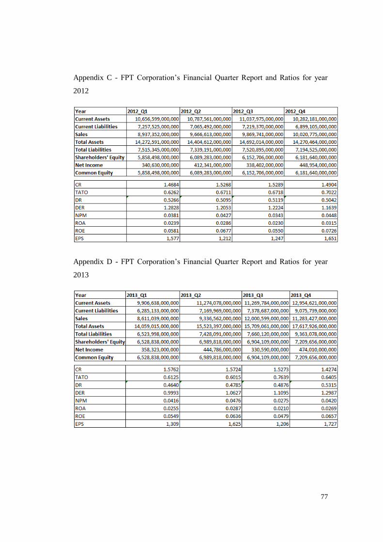
77

Appendix C - FPT Corporation’s Financial Quarter Report and Ratios for year

2012

Appendix D - FPT Corporation’s Financial Quarter Report and Ratios for year

2013

78

Appendix E – SPSS Result of VinGroup

Paired Samples Statistics

Mean N Std. Deviation Std. Error Mean

Pair 1 CRBEFORE 4.129100 8 1.2628873 .4464981

CRAFTER 1.141663 8 .2665696 .0942466

Paired Samples Correlations

N Correlation Sig.

Pair 1 CRBEFORE & CRAFTER 8 -.502 .205

Paired Samples Test

Paired Differences

t

d

f

Sig.

(2-

tailed

) Mean

Std.

Deviation

Std.

Error

Mean

95% Confidence

Interval of the

Difference

Lower Upper

Pai

r 1

CRBEFOR

E -

CRAFTER

2.987437

5

1.415641

2

.500504

7

1.803931

8

4.170943

2

5.96

9 7 .001

79

Paired Samples Statistics

Mean N Std. Deviation Std. Error Mean

Pair 1 TATOBEFORE .038588 8 .0523895 .0185225

TATOAFTER .055263 8 .0398015 .0140719

Paired Samples Correlations

N Correlation Sig.

Pair 1 TATOBEFORE &

TATOAFTER 8 .287 .490

Paired Samples Test

Paired Differences

t df

Sig.

(2-

tailed) Mean

Std.

Deviation

Std. Error

Mean

95% Confidence

Interval of the

Difference

Lower Upper

Pair

1

TATOBEFORE

- TATOAFTER

-

.0166750 .0559524 .0197822

-

.0634524 .0301024

-

.843 7 .427

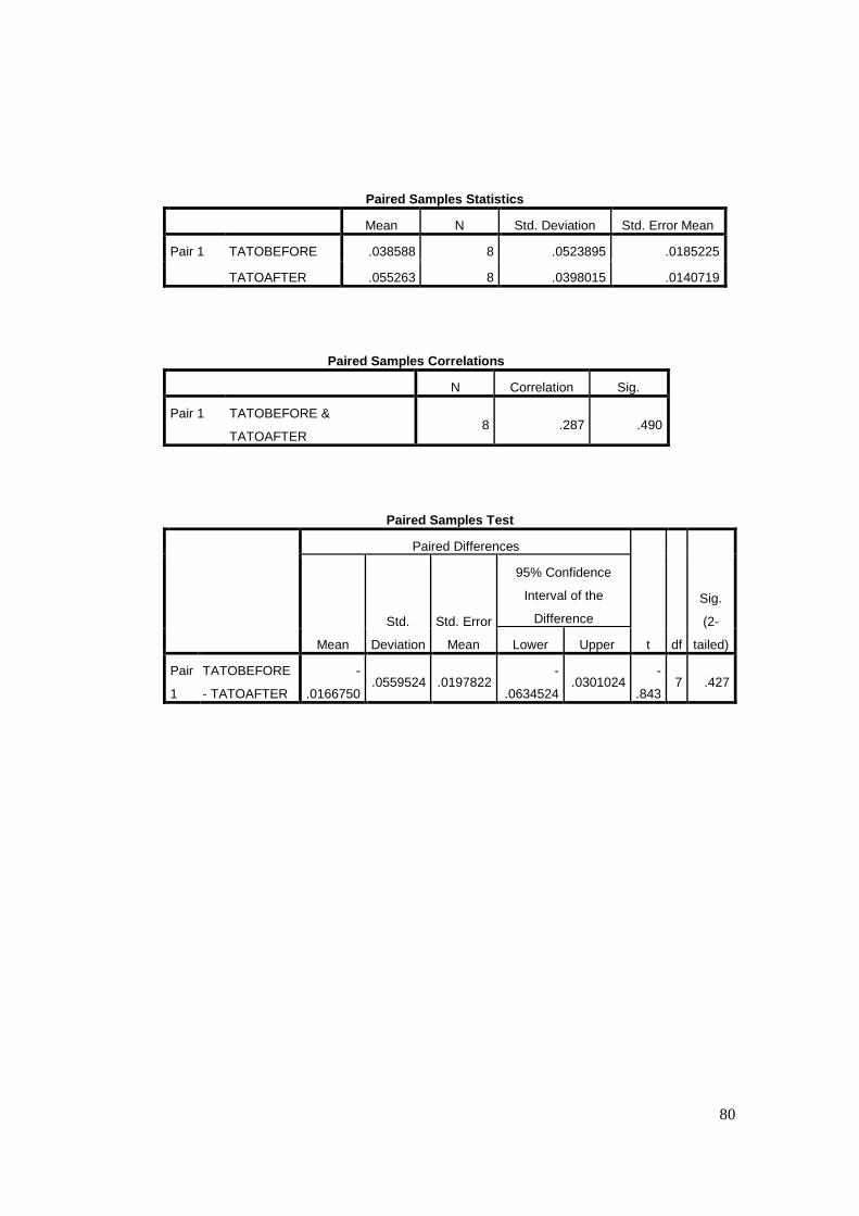
80

Paired Samples Statistics

Mean N Std. Deviation Std. Error Mean

Pair 1 TATOBEFORE .038588 8 .0523895 .0185225

TATOAFTER .055263 8 .0398015 .0140719

Paired Samples Correlations

N Correlation Sig.

Pair 1 TATOBEFORE &

TATOAFTER 8 .287 .490

Paired Samples Test

Paired Differences

t df

Sig.

(2-

tailed) Mean

Std.

Deviation

Std. Error

Mean

95% Confidence

Interval of the

Difference

Lower Upper

Pair

1

TATOBEFORE

- TATOAFTER

-

.0166750 .0559524 .0197822

-

.0634524 .0301024

-

.843 7 .427

81

Paired Samples Statistics

Mean N Std. Deviation Std. Error Mean

Pair 1 DERBEFORE 3.508588 8 1.0658524 .3768357

DERAFTER 3.680688 8 .6364151 .2250067

Paired Samples Correlations

N Correlation Sig.

Pair 1 DERBEFORE & DERAFTER 8 .339 .411

Paired Samples Test

Paired Differences

t df

Sig.

(2-

tailed) Mean

Std.

Deviation

Std.

Error

Mean

95% Confidence

Interval of the

Difference

Lower Upper

Pair

1

DERBEFORE

- DERAFTER

-

.1721000 1.0396903 .3675860

-

1.0413028 .6971028

-

.468 7 .654

82

Paired Samples Statistics

Mean N Std. Deviation Std. Error Mean

Pair 1 NPMBEFORE .562025 8 .4080316 .1442610

NPMAFTER .400888 8 .5587339 .1975423

Paired Samples Correlations

N Correlation Sig.

Pair 1 NPMBEFORE & NPMAFTER 8 -.083 .845

Paired Samples Test

Paired Differences

t df

Sig.

(2-

tailed) Mean

Std.

Deviation

Std. Error

Mean

95% Confidence

Interval of the

Difference

Lower Upper

Pair

1

NPMBEFORE

- NPMAFTER .1611375 .7186397 .2540775

-

.4396603 .7619353 .634 7 .546

83

Paired Samples Statistics

Mean N Std. Deviation Std. Error Mean

Pair 1 ROABEFORE .019600 8 .0281614 .0099566

ROAAFTER .018100 8 .0207882 .0073497

Paired Samples Correlations

N Correlation Sig.

Pair 1 ROABEFORE & ROAAFTER 8 -.278 .505

Paired Samples Test

Paired Differences

t df

Sig.

(2-

tailed) Mean

Std.

Deviation

Std. Error

Mean

95% Confidence

Interval of the

Difference

Lower Upper

Pair

1

ROABEFORE

- ROAAFTER .0015000 .0393768 .0139218

-

.0314198 .0344198 .108 7 .917

84

Paired Samples Statistics

Mean N Std. Deviation Std. Error Mean

Pair 1 ROEBEFORE .093100 8 .1287092 .0455056

ROEAFTER .076462 8 .0807770 .0285590

Paired Samples Correlations

N Correlation Sig.

Pair 1 ROEBEFORE & ROEAFTER 8 -.325 .432

Paired Samples Test

Paired Differences

t df

Sig.

(2-

tailed) Mean

Std.

Deviation

Std. Error

Mean

95% Confidence

Interval of the

Difference

Lower Upper

Pair

1

ROEBEFORE

- ROEAFTER .0166375 .1727950 .0610923

-

.1278227 .1610977 .272 7 .793

85

Paired Samples Statistics

Mean N Std. Deviation Std. Error Mean

Pair 1 EPSBEFORE 1468.38 8 2272.036 803.286

EPSAFTER 1309.75 8 1388.468 490.898

Paired Samples Correlations

N Correlation Sig.

Pair 1 EPSBEFORE & EPSAFTER 8 -.274 .512

Paired Samples Test

Paired Differences

t df

Sig.

(2-

tailed) Mean

Std.

Deviation

Std. Error

Mean

95% Confidence

Interval of the

Difference

Lower Upper

Pair

1

EPSBEFORE

- EPSAFTER 158.625 2969.473 1049.867 -2323.917 2641.167 .151 7 .884

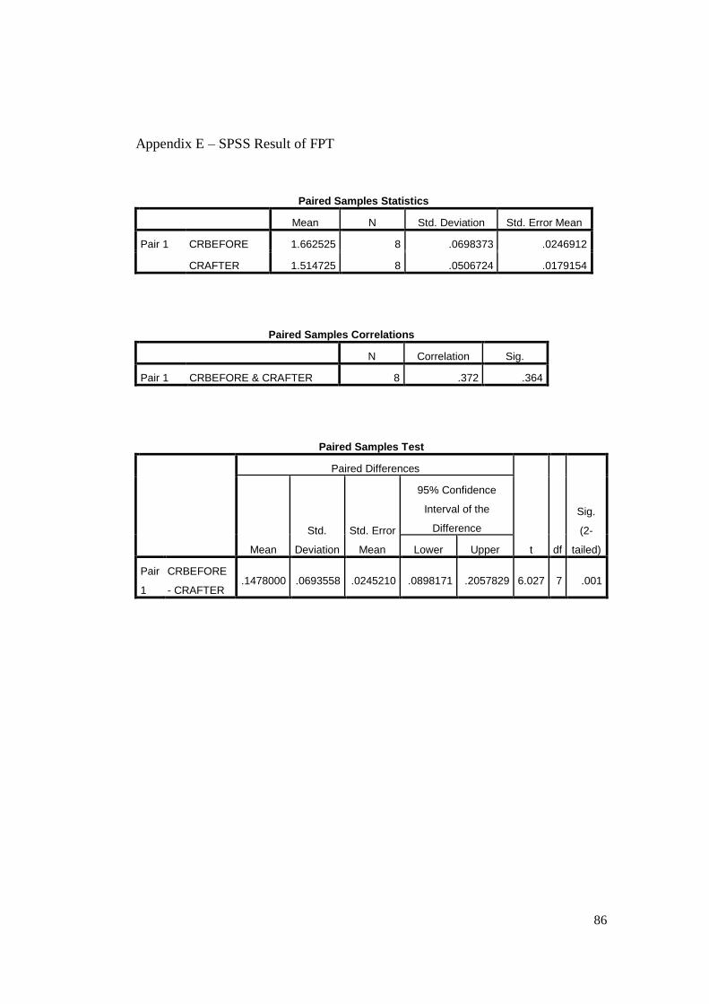
86

Appendix E – SPSS Result of FPT

Paired Samples Statistics

Mean N Std. Deviation Std. Error Mean

Pair 1 CRBEFORE 1.662525 8 .0698373 .0246912

CRAFTER 1.514725 8 .0506724 .0179154

Paired Samples Correlations

N Correlation Sig.

Pair 1 CRBEFORE & CRAFTER 8 .372 .364

Paired Samples Test

Paired Differences

t df

Sig.

(2-

tailed) Mean

Std.

Deviation

Std. Error

Mean

95% Confidence

Interval of the

Difference

Lower Upper

Pair

1

CRBEFORE

- CRAFTER .1478000 .0693558 .0245210 .0898171 .2057829 6.027 7 .001

87

Paired Samples Statistics

Mean N Std. Deviation Std. Error Mean

Pair 1 TATOBEFORE 1.086988 8 .2429099 .0858816

TATOAFTER .661213 8 .0534896 .0189114

Paired Samples Correlations

N Correlation Sig.

Pair 1 TATOBEFORE & TATOAFTER 8 .383 .349

Paired Samples Test

Paired Differences

t df

Sig.

(2-

tailed) Mean

Std.

Deviation

Std.

Error

Mean

95% Confidence

Interval of the

Difference

Lower Upper

Pair

1

TATOBEFORE

- TATOAFTER .4257750 .2278342 .0805516 .2353008 .6162492 5.286 7 .001

88

Paired Samples Statistics

Mean N Std. Deviation Std. Error Mean

Pair 1 DRBEFORE .554938 8 .0692463 .0244823

DRAFTER .501725 8 .0234140 .0082781

Paired Samples Correlations

N Correlation Sig.

Pair 1 DRBEFORE & DRAFTER 8 -.413 .309

Paired Samples Test

Paired Differences

t df

Sig.

(2-

tailed) Mean

Std.

Deviation

Std. Error

Mean

95% Confidence

Interval of the

Difference

Lower Upper

Pair

1

DRBEFORE

- DRAFTER .0532125 .0817450 .0289012 -.0151280 .1215530 1.841 7 .108

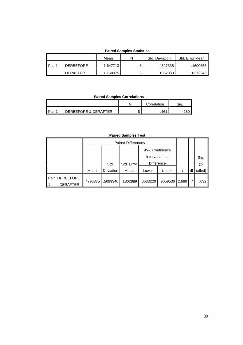
89

Paired Samples Statistics

Mean N Std. Deviation Std. Error Mean

Pair 1 DERBEFORE 1.647713 8 .4527335 .1600655

DERAFTER 1.168075 8 .1052880 .0372249

Paired Samples Correlations

N Correlation Sig.

Pair 1 DERBEFORE & DERAFTER 8 -.461 .250

Paired Samples Test

Paired Differences

t df

Sig.

(2-

tailed) Mean

Std.

Deviation

Std. Error

Mean

95% Confidence

Interval of the

Difference

Lower Upper

Pair

1

DERBEFORE

- DERAFTER .4796375 .5099340 .1802889 .0533220 .9059530 2.660 7 .032

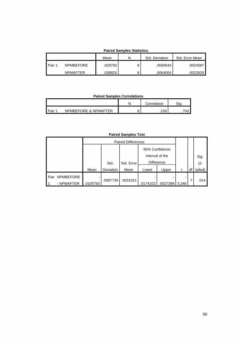
90

Paired Samples Statistics

Mean N Std. Deviation Std. Error Mean

Pair 1 NPMBEFORE .029750 8 .0069543 .0024587

NPMAFTER .039825 8 .0064004 .0022629

Paired Samples Correlations

N Correlation Sig.

Pair 1 NPMBEFORE & NPMAFTER 8 .139 .743

Paired Samples Test

Paired Differences

t df

Sig.

(2-

tailed) Mean

Std.

Deviation

Std. Error

Mean

95% Confidence

Interval of the

Difference

Lower Upper

Pair

1

NPMBEFORE

- NPMAFTER

-

.0100750 .0087739 .0031021

-

.0174102

-

.0027398

-

3.248 7 .014

91

Paired Samples Statistics

Mean N Std. Deviation Std. Error Mean

Pair 1 ROABEFORE .031513 8 .0070833 .0025043

ROAAFTER .026138 8 .0034562 .0012220

Paired Samples Correlations

N Correlation Sig.

Pair 1 ROABEFORE & ROAAFTER 8 -.080 .851

Paired Samples Test

Paired Differences

t df

Sig.

(2-

tailed) Mean

Std.

Deviation

Std. Error

Mean

95% Confidence

Interval of the

Difference

Lower Upper

Pair

1

ROABEFORE

- ROAAFTER .0053750 .0081250 .0028726

-

.0014177 .0121677 1.871 7 .104

92

Paired Samples Statistics

Mean N Std. Deviation Std. Error Mean

Pair 1 ROEBEFORE .089662 8 .0121089 .0042811

ROEAFTER .060687 8 .0081130 .0028684

Paired Samples Correlations

N Correlation Sig.

Pair 1 ROEBEFORE & ROEAFTER 8 .234 .577

Paired Samples Test

Paired Differences

t df

Sig.

(2-

tailed) Mean

Std.

Deviation

Std. Error

Mean

95% Confidence

Interval of the

Difference

Lower Upper

Pair

1

ROEBEFORE

- ROEAFTER .0289750 .0129039 .0045622 .0181871 .0397629 6.351 7 .000