Embed Size (px)
Citation preview

The APA has copyright on this article. When published, it can be found at:
http://www.apa.org/pubs/journals/xhp/index.aspx
This article may not exactly replicate the final version published in the APA journal. It is not
the copy of record.

Weighted integration suggests that visual and tactile signals provide
independent estimates about duration
Danny M. Ball 1, Derek H. Arnold 2 & Kielan Yarrow 1*
1 Cognitive Neuroscience Research Unit, Department of Psychology, City, University of London,
London, U.K.
2 School of Psychology, The University of Queensland, Brisbane, Australia
* Author for correspondence:
Kielan Yarrow,
Rhind Building,
City, University of London,
Northampton Square,
London EC1V 0HB
Tel: +44 (0)20 7040 8530
Fax: +44 (0)20 7040 8580
Email: [email protected]

Abstract
Humans might possess either a single (amodal) internal clock, or multiple clocks for different
sensory modalities. Sensitivity could be improved by the provision of multiple signals. Such
improvements can be predicted quantitatively, assuming estimates are combined by summation, a
process described as optimal when summation is weighted in accordance with the variance
associated with each of the initially independent estimates. We assessed this possibility for visual
and tactile information regarding temporal intervals. In Experiment 1, 12 musicians and 12 non-
musicians judged durations of 300 and 600 ms, compared to test values spanning these standards.
Bimodal precision increased relative to unimodal conditions, but not by the extent predicted by
optimally weighted summation. In Experiment 2, six musicians and six other participants each judged
six standards, ranging from 100 ms to 600 ms, with conflicting cues providing a measure of the
weight assigned to each sensory modality. A weighted integration model best fitted these data, with
musicians more likely to select near-optimal weights than non-musicians. Overall, data were
consistent with the existence of separate visual and tactile clock components at either the
counter/integrator or memory stages. Independent estimates are passed to a decisional process, but
not always combined in a statistically optimal fashion.
Statement of public significance
We are able to judge the duration of events as they unfold (e.g. the time for which
somebody holds our gaze). Sometimes, this information is conveyed to several of our senses at once
(e.g. both seeing and feeling the duration of a caress). Theorists argue about whether time intervals
are calculated separately for each sense, or rely on a common centralised timer. This study suggests
that when people experience the duration of events via both vision and touch, they gain a
multisensory benefit, performing better than when they receive just visual or just tactile stimulation.
This kind of benefit can only accrue if time is first estimated independently within each sense,
suggesting that separate timers exist.

Humans and other animals express their ability to time intervals through a wide variety of
behaviours. In the lab, this ability is often assessed by requiring experimental participants to make
judgments about the duration of events. However, our knowledge regarding the neurocognitive
bases of these judgments remains hazy. One debate concerns the centralised versus distributed
nature of the hypothetical internal clock or clocks (Ivry & Schlerf, 2008; Ivry & Spencer, 2004). On
the one hand, it is possible that all time-dependent behaviours rely on a single multimodal timer,
through which a wide variety of sensory information is routed. On the other, it may be that there are
different clocks for different purposes, for example for sensory versus motor timing (Keele, Pokorny,
Corcos, & Ivry, 1985; Marinovic & Arnold, 2012), implicit versus explicit timing (Coull & Nobre, 2008),
short versus long interval timing (Lewis & Miall, 2003; Rammsayer, 1999), and for timing in different
sensory modalities (Eijkman & Vendrik, 1965; Merchant, Zarco, & Prado, 2008).
The single versus multiple clock debate has received some attention from psychophysical
studies focussed on a single modality. For example, in both vision and touch, adaptation at a single
spatial location can selectively affect subsequent interval judgments at that location, and not others
(Johnston, Arnold, & Nishida, 2006; Watanabe, Amemiya, Nishida, & Johnston, 2010) perhaps
implying multiple spatially localised timing mechanisms. However, there appears to be little or no
statistical benefit from providing multiple visual inputs (which might reasonably be averaged to
derive a more precise estimate of duration; see Ayhan, Revina, Bruno, & Johnston, 2012; and
Morgan, Giora, & Solomon, 2008). This suggests either a severe attentional bottleneck for visual
interval timing, or a single centralised mechanism that is modulated by localised visual inputs.
Further evidence pertinent to this debate comes from the multimodal literature. For
example, the repetition of a visual stimulus with a particular duration can generate repulsive after
effects, which can be measured when an adapted visual stimulus is compared to an auditory
reference (and vice versa following auditory adaptation; see Heron et al., 2012). This implies that
intervals in one modality either specifically, or disproportionately, adapt time perception within that
same modality, suggesting modality-specific clocks. However, training on interval timing tasks in one
modality can improve performance when precision is tested in a second sensory modality (Bartolo &
Merchant, 2009; Bratzke, Seifried, & Ulrich, 2012; Nagarajan, Blake, Wright, Byl, & Merzenich, 1998;
but see Lapid, Ulrich, & Rammsayer, 2009), instead suggesting a shared timing resource.
One behavioural method that can provide insights regarding the existence of multiple clocks
involves assessing performance in unimodal conditions, and then seeking evidence for a bimodal
improvement in precision resulting from the combination of initially independent sensory estimates
(Macmillan & Creelman, 2005; Treisman, 1998). A widely adopted model of this process posits that
information is combined via an optimally weighted summation process, known as maximum

likelihood estimation (MLE) integration (Ernst & Banks, 2002; van Beers, Sittig, & Gon, 1999). In this
case, each initially independent estimate receives a weighting in inverse proportion to its precision
(i.e. the uncertainty regarding its accuracy). This model is typically contrasted with a less
sophisticated strategy, in which observers rely on estimates arising from the modality that generally
provides more precise information regarding the pertinent question. For example, auditory signals
might dominate timing judgments, as auditory processing is typically more precise in the time
domain than is vision.
The two computational strategies outlined above reflect just two possibilities. It is possible
to envisage many intermediate models. For example, observers might be limited to using a single
estimate, but may select this idiosyncratically, selecting their own most precise modality for a given
experimental condition. Alternatively, they might make use of two modalities without actually
averaging their estimates (e.g. via the max rule of probability summation from classic signal
detection theory, in which both sensory estimates are evaluated and a decision is triggered if either
reaches a criterion value). We could also consider an averaging of signals without optimal weighting
of sensory evidence, or an averaging of signals containing partially correlated (rather than fully
independent) sources of noise. In all cases, support for one or another of these models over others
could be instructive regarding whether more than one independent estimate of duration has been
derived on each experimental trial. Hence testing task performance in both unimodal and bimodal
interval timing tasks could provide rich insights regarding the possible existence of multiple internal
clocks.
To date, several studies have assessed cue combination for duration judgments via changes
in bimodal precision1. Results have been mixed. The issue was, to our knowledge, first considered by
Eijkman and Vendrik (1965). They applied detection-theoretic models to data from a filled duration
discrimination task with auditory, visual and audiovisual conditions. Observers attempted to detect
deviations from a standard duration of one second. Bimodal performance was essentially identical to
performance in the unimodal conditions (which were of similar difficulty to one another). The
authors therefore concluded that noise had been perfectly correlated for unimodal signals,
consistent with a single multimodal duration processor. This conclusion was at odds with the one
they reached regarding the detection of intensity increments, where noise appeared uncorrelated
(yielding bimodal enhancement). It also sits uncomfortably with findings pertaining to the
summation of signals encoded by a single mechanism, such as when two spots of light are encoded
1 We focus on predictions regarding precision as these are generally considered to provide more compelling
evidence of cue combination, specifically when bimodal precision exceeds that of the best contributing
unimodal signal.

by a single sensory detector – here sensitivity doubles, as if noise accrues only after signal
combination.
More recent work has tended not to prioritise implications for models of the internal clock,
focussing instead on establishing (or questioning) the general applicability of the MLE model of cue
combination. For example, Burr, Banks, and Morrone (2009) found partial (but sub-optimal)
integration for empty intervals demarcated by audiovisual stimuli. A follow-up developmental study
from the same group showed little evidence of integration (Gori, Sandini, & Burr, 2012). Around the
same time, Van Wassenhove, Buonomano, Shimojo, and Shams (2008) investigated integration as
part of a series of experiments focussing on the biasing effects of looming and receding stimuli for
durations signalled by filled visual, auditory and bimodal signals. The pertinent data (shown in their
Figures S3 and 5) suggest partial, but sub-optimal, facilitation in the bimodal case.
Some studies have tested relevant conditions without attempting to apply formal models of
bimodal integration. For example, Gamache and Grondin (2010) illustrate a trend suggestive of
multisensory facilitation in a subset of their unimodal and audiovisual conditions, which included
matched auditory and visual standard durations. By contrast, a recent study testing high-functioning
Autistics and matched controls on an auditory, visual and audiovisual interval comparison task
obtained bimodal thresholds that were very similar to those of the best unimodal condition
(Lambrechts, Yarrow & Gaigg, submitted). A classic paper comparing auditory and visual time
perception alongside audiovisual conditions (Walker & Scott, 1981) similarly showed no evidence for
bimodal precision exceeding the best unimodal condition, a tendency we have also noted in several
more recent publications (e.g. Rattat & Picard, 2012).
Two studies have used reproduction tasks and explicitly tested how auditory and
tactile/motor (Shi, Ganzenmüller, & Müller, 2013) or visual and tactile (Tomassini, Gori, Burr,
Sandini, & Morrone, 2011) time estimates are combined. These reported a partial integration and a
very limited integration respectively (although it is difficult to properly partition sources of noise
when using a reproduction task, in order to derive appropriate model predictions). However,
Hartcher-O'Brien, Di Luca, and Ernst (2014) have recently reported optimally weighted integration
for filled audiovisual stimuli of around 500 ms duration using an interval comparison task, and have
suggested that this should be generally obtained for filled-interval stimuli.
Given the mixed results, and the pertinence of cue combination studies to the debate
regarding the architecture of the human timing system, further research investigating bimodal
integration for duration judgments seems warranted. One issue particularly affecting audiovisual
research on this topic is that experimenters have often used either clearly suprathreshold stimuli (in
which case temporal sensitivity tends not to be well matched between auditory and visual stimuli,
and predicted facilitation is therefore limited, reducing experimental power; e.g. Lambrechts,
Yarrow & Gaigg, submitted) or have degraded stimuli by introducing masking noise (in which case it
seems likely that the equalisation of sensitivity that is achieved will reflect problems detecting
temporal cues (presumably stimulus onsets and offsets) rather than a change in the scalar noise that
usually dominates interval judgments; e.g. Hartcher-O'Brien, Di Luca, and Ernst, 2014). For both of
these reasons, we chose to investigate integration of visual and tactile signals, which seemed more
likely to give rise to similar levels of precision, even for non-degraded suprathreshold stimuli (Jones,
Poliakoff, & Wells, 2009). We also investigated integration in individuals with differing levels of
timing expertise, in order to determine whether integration might be experience dependent,
operationalising this factor by assessing samples of participants with or without extensive musical
training.
Experiment 1
Methods
Participants
Twenty-seven participants were tested, 12 musicians (each of whom had received
Associated Board of the Royal Schools of Music (ABRSM) Grade 8 qualifications) and 15 non-
musicians (with no prior experience of musical training). Three non-musicians were excluded from
the final analysis as they did not perform significantly above chance in one or more conditions (see
data analysis, below). The final sample therefore consisted of 12 musicians, 9 male, with a mean age
of 26 years (from multiple disciplines of musical training: 3 percussionists, 2 brass players and 7
string instrumentalists), and 12 non-musicians, 4 male, with a mean age of 23 years. Each participant
provided informed consent, with testing procedures approved by the Department of Psychology
research ethics committee at City, University of London.
Apparatus and stimuli
The experiment was controlled by a Visual C++ program running on a PC interfaced with a 16
bit A/D card (National Instruments X-series PCIe-6323) generating digitized signals at 44.1 MHz.
Visual stimuli were presented with a red LED (~0.5 degrees visual angle in diameter, ~60 mcd point
source). It was placed on a desk to the left of a monitor approximately 50 cm from the participant.
Vibrotactile stimuli were 200 Hz sine waves. They were delivered using a piezoelectric ceramic disc

covered with a rubber sheath approximately 1 cm in diameter, powered by a bespoke amplifier, and
were virtually silent. The piezoelectric disc was pinched between the forefinger and thumb, which
rested on the desk close to (~10 cm) but not obscuring the LED.
Design
A 2x2x3 mixed factorial design included repeated measures on the last two factors. Factor
one was the level of participant expertise: Musicians or non-musicians. Factor two was the standard
duration: 300ms or 600ms. The order of standards was randomized (without replacement) in each
block. The final factor was stimulus modality: Unimodal tactile, unimodal visual, and bimodal. This
factor was blocked, and block order was counterbalanced across each set of six participants. In all,
participants completed 3 blocks (600 trials).
Procedure
Participants sat at a desk with the computer screen and keyboard directly in front of them.
The piezoelectric disc was held using the left hand in all conditions, including the unimodal visual
condition. The right hand was used to indicate judgments using left or right arrow keys (or delete to
cancel a trial due to an attentional lapse). Participants received 10 practice trials to familiarize
themselves with the procedure in each condition, before beginning a block of 200 trials. No feedback
on performance was given.
On each trial, a standard duration of either 300ms or 600ms was presented, followed by a
1000 ms inter-stimulus interval that proceeded the onset of a test stimulus (see Figure 1). The test
stimulus was drawn at random from an adaptive distribution that was initially uniform (75-125% of
the standard duration in 5% increments) but which could potentially expand to range from 25-175%
of the standard duration: It was updated after each accepted trial according to the generalised Pólya
urn procedure (Rosenberger & Grill, 1997) in order to sample the psychometric function in an
efficient manner.
Following each test presentation, participants reported which interval had seemed longer,
the first or second. We used this interval comparison task as it should provide clean estimates of
sensory noise for the purposes of deriving model-based predictions about integration.2
Data Analysis
2 As we noted earlier, it is challenging to properly partition sources of variance from some timing tasks, such as
reproduction, for the purposes of fitting models of multisensory integration. We revisit this issue in the
General Discussion.

For each participant, the proportion of tests judged longer than the standard was
determined at each test duration in each condition. Data were imported into Matlab (The
MathWorks Inc) and maximum-likelihood fitted to Cumulative Gaussian psychometric functions
(with a fixed 1% lapse rate assumed). Points of subjective equality (PSE) and 84% thresholds (σ) were
then estimated from these psychometric functions. PSE estimates represent the test value at which
tests were judged to be longer than standard with a 0.5 probability. However, our main interest here
was the threshold, which was estimated as the difference between test durations yielding “longer”
judgments with probabilities 0.5 and 0.84. Under a standard observer model with Gaussian decision
noise, this represents the standard deviation of the noise contributing to that decision.
Data were additionally fitted using a one-parameter horizontal line. A straight line would
best fit data if a participant was randomly guessing with some unknown response bias for each key.
Participants were retained only when the cumulative Gaussian psychometric function fitted their
data significantly better than a straight line (p<0.01) in all conditions, assessed by comparing the
difference in best-fitting model deviances against an appropriate chi-squared distribution
(Wichmann & Hill, 2001).
Data from unimodal conditions were used to form predictions for both the optimally
weighted integration (MLE) model and for a non-integration model, assuming each observer relied
entirely on the sensory signal producing their highest precision for that particular condition. For the
MLE model, the prediction regarding the bimodal threshold (σTV) is well-established (Ernst & Banks,
2002):
(1) ���� = ���
�����
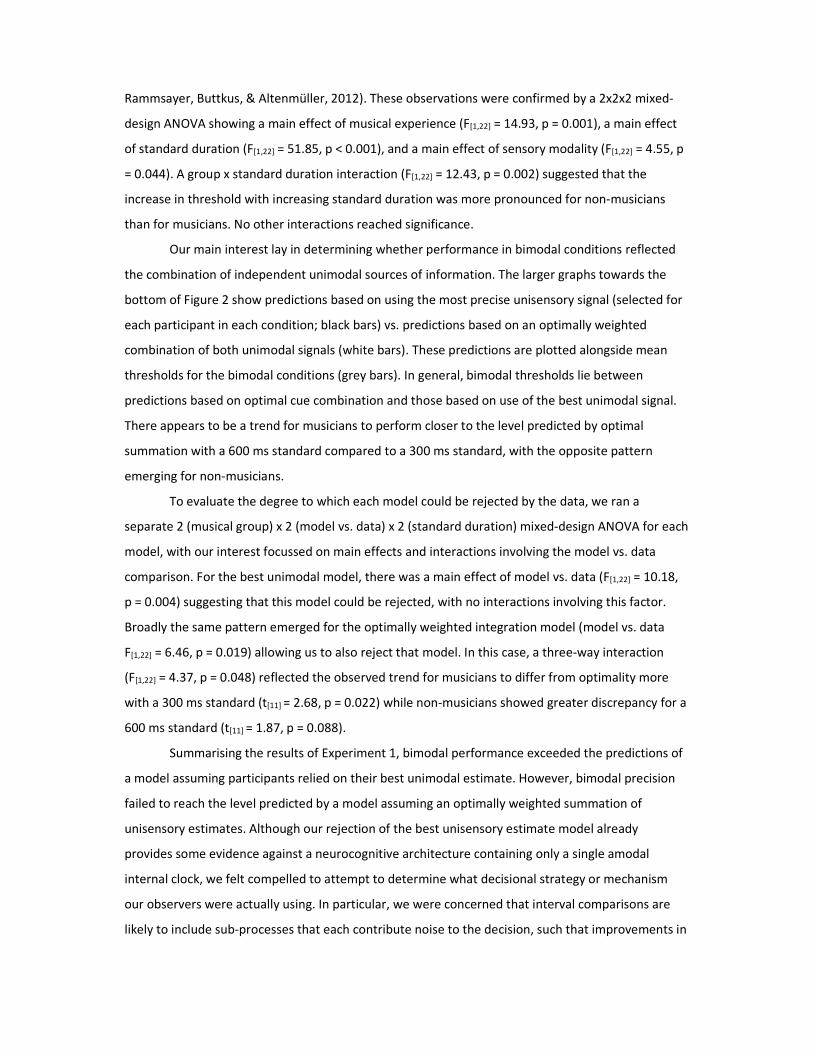
Results and Discussion
Figure 2 shows mean threshold (σ) estimates for musicians and non-musicians in all
conditions, alongside model predictions. The inset graphs at the top of the figure present data from
the unimodal tactile and visual conditions. Importantly, average performance was similar for
vibrotactile and visual signals, providing scope for the combination of information to result in
detectable performance improvements in bimodal conditions (relative to relying on one or other
sensory modality alone). However, visual thresholds were generally slightly higher than tactile
thresholds. As expected, unimodal thresholds increased near linearly with increasing standard
duration (i.e. the scalar property of time) and were higher for non-musicians than for musicians,
consistent with many previous reports (e.g. Cicchini, Arrighi, Cecchetti, Giusti, & Burr, 2012;
Rammsayer, Buttkus, & Altenmüller, 2012). These observations were confirmed by a 2x2x2 mixed-
design ANOVA showing a main effect of musical experience (F[1,22] = 14.93, p = 0.001), a main effect
of standard duration (F[1,22] = 51.85, p < 0.001), and a main effect of sensory modality (F[1,22] = 4.55, p
= 0.044). A group x standard duration interaction (F[1,22] = 12.43, p = 0.002) suggested that the
increase in threshold with increasing standard duration was more pronounced for non-musicians
than for musicians. No other interactions reached significance.
Our main interest lay in determining whether performance in bimodal conditions reflected
the combination of independent unimodal sources of information. The larger graphs towards the
bottom of Figure 2 show predictions based on using the most precise unisensory signal (selected for
each participant in each condition; black bars) vs. predictions based on an optimally weighted
combination of both unimodal signals (white bars). These predictions are plotted alongside mean
thresholds for the bimodal conditions (grey bars). In general, bimodal thresholds lie between
predictions based on optimal cue combination and those based on use of the best unimodal signal.
There appears to be a trend for musicians to perform closer to the level predicted by optimal
summation with a 600 ms standard compared to a 300 ms standard, with the opposite pattern
emerging for non-musicians.
To evaluate the degree to which each model could be rejected by the data, we ran a
separate 2 (musical group) x 2 (model vs. data) x 2 (standard duration) mixed-design ANOVA for each
model, with our interest focussed on main effects and interactions involving the model vs. data
comparison. For the best unimodal model, there was a main effect of model vs. data (F[1,22] = 10.18,
p = 0.004) suggesting that this model could be rejected, with no interactions involving this factor.
Broadly the same pattern emerged for the optimally weighted integration model (model vs. data
F[1,22] = 6.46, p = 0.019) allowing us to also reject that model. In this case, a three-way interaction
(F[1,22] = 4.37, p = 0.048) reflected the observed trend for musicians to differ from optimality more
with a 300 ms standard (t[11] = 2.68, p = 0.022) while non-musicians showed greater discrepancy for a
600 ms standard (t[11] = 1.87, p = 0.088).
Summarising the results of Experiment 1, bimodal performance exceeded the predictions of
a model assuming participants relied on their best unimodal estimate. However, bimodal precision
failed to reach the level predicted by a model assuming an optimally weighted summation of
unisensory estimates. Although our rejection of the best unisensory estimate model already
provides some evidence against a neurocognitive architecture containing only a single amodal
internal clock, we felt compelled to attempt to determine what decisional strategy or mechanism
our observers were actually using. In particular, we were concerned that interval comparisons are
likely to include sub-processes that each contribute noise to the decision, such that improvements in

precision might reflect optimal integration for some, but not all sources of noise. This would clearly
affect conclusions regarding any putative clock architecture. In particular, we wondered if
participants might be integrating estimates of event onset and offset (likely affected by clock switch
latency variability) without integrating estimates derived mainly from the integration of the
intervening time (often thought of as a clock count), or vice versa.
To address this issue, we designed a second experiment in which six standard durations
ranging from 100 to 600 ms were used. This allowed us to apply a slope analysis method (Ivry &
Hazeltine, 1995; Narkiewicz, Lambrechts, Eichelbaum, & Yarrow, 2015) in order to decompose
judgment variability into a component contributed by non-scalar operations (including starting and
stopping the clock) and a scalar component that grows with the duration being timed (reflecting
counter and/or memory processes). With separate estimates, we were able to make predictions
regarding the integration of one but not both sources of noise. We also took the opportunity to
introduce a small discrepancy between tactile and visual components of our standard stimuli. This
approach is commonly used (e.g. Ernst & Banks, 2002; Ley, Haggard, & Yarrow, 2009) in order to
estimate the weight being assigned to each sensory modality, and thus provide a further means of
assessing the predictions of weighted integration models.
Experiment 2
Methods
Methods were identical to those used in the first experiment, with the following exceptions.
Participants
Thirteen participants were tested including 7 musicians (with ABRSM Grade 8 qualifications)
and 6 psychophysical observers (i.e. lab members from local groups recruited specifically because
they had experience participating in experimental tasks of this kind).3 One musician completed only
a few blocks before being excluded from further participation, as they reported great difficulty
detecting the vibrotactile stimulus (confirmed by their very poor performance in tactile conditions).
3 Of course, strictly, all of our participants could be considered psychophysical observers. We refer to this
group as psychophysical observers, as opposed to non-musicians, for two reasons. Firstly, it contextualises
their strong timing performance; they were distinct from the musician group in another important respect, not
just in being less musically expert. Secondly, we did not exclude participants from this group for having some
degree of past musical training (although their musical attainment was in no sense equivalent to our musician
group). In fact, in Experiment 2 we recruited musicians not so much because we expected them to be
different, but rather because Experiment 1 had indicated that this group would perform timing tasks well.
The final sample therefore consisted of 6 musicians (3 pianists, 2 string instrumentalists, 1 brass
player), all female, with a mean age of 22 years, and 6 psychophysical observers, 4 female, with a
mean age of 29 years.
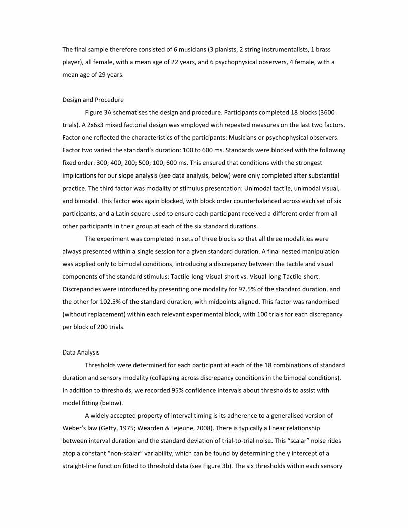
Design and Procedure
Figure 3A schematises the design and procedure. Participants completed 18 blocks (3600
trials). A 2x6x3 mixed factorial design was employed with repeated measures on the last two factors.
Factor one reflected the characteristics of the participants: Musicians or psychophysical observers.
Factor two varied the standard’s duration: 100 to 600 ms. Standards were blocked with the following
fixed order: 300; 400; 200; 500; 100; 600 ms. This ensured that conditions with the strongest
implications for our slope analysis (see data analysis, below) were only completed after substantial
practice. The third factor was modality of stimulus presentation: Unimodal tactile, unimodal visual,
and bimodal. This factor was again blocked, with block order counterbalanced across each set of six
participants, and a Latin square used to ensure each participant received a different order from all
other participants in their group at each of the six standard durations.
The experiment was completed in sets of three blocks so that all three modalities were
always presented within a single session for a given standard duration. A final nested manipulation
was applied only to bimodal conditions, introducing a discrepancy between the tactile and visual
components of the standard stimulus: Tactile-long-Visual-short vs. Visual-long-Tactile-short.
Discrepancies were introduced by presenting one modality for 97.5% of the standard duration, and
the other for 102.5% of the standard duration, with midpoints aligned. This factor was randomised
(without replacement) within each relevant experimental block, with 100 trials for each discrepancy
per block of 200 trials.
Data Analysis
Thresholds were determined for each participant at each of the 18 combinations of standard
duration and sensory modality (collapsing across discrepancy conditions in the bimodal conditions).
In addition to thresholds, we recorded 95% confidence intervals about thresholds to assist with
model fitting (below).
A widely accepted property of interval timing is its adherence to a generalised version of
Weber’s law (Getty, 1975; Wearden & Lejeune, 2008). There is typically a linear relationship
between interval duration and the standard deviation of trial-to-trial noise. This “scalar” noise rides
atop a constant “non-scalar” variability, which can be found by determining the y intercept of a
straight-line function fitted to threshold data (see Figure 3b). The six thresholds within each sensory

modality were therefore fitted with a two-parameter model, with the intercept constrained to be ≥
0. To avoid undue influence from poorly estimated thresholds (and to appropriately weight the more
precisely estimated thresholds typically observed at lower standard durations) we utilised a
maximum-likelihood (rather than least squares) fit, assuming a Gaussian data model with separate
scale parameters reflecting uncertainty for each threshold (based on their 95% confidence intervals).
In addition to an estimate of non-scalar variability, this fitting procedure provided a set of cleaned
data points (i.e. the scalar model’s predicted values) which were used in all subsequent calculations
and analyses.4
For this experiment, we estimated thresholds in all conditions, in addition to the weights
assigned to the tactile modality in bimodal conditions. Empirical weights were derived by fitting
cumulative Gaussians to data collapsed across all six standard durations (with the test values
normalised by their standard durations and expressed as percentages) but separated on the basis of
the discrepancy within the standard stimulus (tactile-long-visual-short vs. visual-long-tactile-short).
The PSEs from these fits were differenced, and this difference scaled to generate an empirical
estimate of tactile weight:
(2) �� = 0.5 + ���������������
These empirical weights were used in modelling (see below) and also to test the optimally
weighted integration model. For the MLE model, the prediction regarding optimal weights is well-
established (Ernst & Banks, 2002):
(3) �� =�
����
For the purposes of this prediction, we used the average of thresholds at each standard
duration, normalised by their respective standards.
Data from the unimodal conditions were also used to form predictions for six different
models regarding bimodal thresholds. In addition to the optimally weighted integration and best
4 We consider these cleaned data preferable to the raw data as they make best use of well-established
properties of time perception to reduce measurement noise. We return to this issue in the discussion. Note,
however, that it would have also been difficult to have proceeded from the raw data in our analyses, as two of
our twelve participants produced large and very poorly estimated thresholds in a small subset of conditions,
despite generally performing well. With 18 conditions per participant, we preferred not to reject entire
participants on the basis of one or two poor estimates, and our fitting procedure made this feasible.

unimodal predictions (outlined in Experiment 1), we calculated predictions for two hybrid models, in
which non-scalar variance was integrated optimally and scalar variance came from the best
unimodal stimulus, or vice versa. We also considered a model utilising the max rule of probability
summation: Observers were assumed to have access to both unimodal estimates, and to compare
tests to standards in both cases, responding longer if either unimodal test exceeded its
corresponding standard. Finally, we tested a model of weighted integration (i.e. averaging) but with
weights based not on the optimal selection strategy described in Equation 3, but rather derived
empirically (as described in Equation 2). Predictions for these final two models were based on
Matlab simulations, with simulated data subjected to a cumulative Gaussian fit (in a similar manner
to our real data) to generate predicted thresholds (cf. Treisman, 1998).
Our main inferential analysis again used ANOVA, but to assist data visualisation and
inference at the level of the individual participant, we also made use of non-parametric
bootstrapping, using the bias-corrected method with 1999 bootstrap resamples. For bootstrap
inference, we calculated 95% confidence intervals on the difference between estimates from pairs of
conditions.
Results and Discussion
In Experiment 2 we included a small discrepancy between the vibrotactile and visual
components of our bimodal standards. This allowed us to estimate the degree to which each
participant relied on tactile (vs. visual) information to inform their decisions. Estimated tactile
weights are plotted in Figure 4a, against weights that would be predicted for optimally weighted cue
combination (based on performance in unimodal conditions). Across the sample as a whole, we did
not obtain the predicted linear relationship (with a slope of 1.0) between optimal and empirical
tactile weights (r = 0.186, p > 0.05). However, it is apparent that our musician subgroup (black
circles) showed a much greater degree of optimality in their empirically derived tactile weights than
did our psychophysical observers (white circles).
The additional standard durations and empirical estimates of tactile weights available in
Experiment 2 allowed us to consider a wider range of model predictions regarding bimodal
thresholds. Figure 4b plots the predictions of several models (in the leftmost column of graphs) for
the group as a whole, and also separately for each subgroup. It is clear that for these participants,
relying on the most precise (i.e. best) unisensory modality would generate very similar predictions to
using this same strategy supplemented by the optimally weighted integration of only non-scalar
sources of independent information (e.g. clock onset/offset times) or indeed to making use of both

modalities independently via a max response rule (i.e. probability summation).5 Meanwhile,
predictions from the optimally weighted integration model are very close to those of a model in
which only scalar sources of independent information are combined via optimal weighting. Finally,
weighted combination based on empirically derived tactile weights falls midway between these
groups of predictions, at least for the sample as a whole. However, this form of cue combination
provides near-optimal predictions about threshold for the musician subset (as they appeared to
select near-optimal weights) but predicts thresholds similar to using the best unimodal stimulus for
the non-musician subset (who appeared to give an inappropriately high weighting to the vibrotactile
stimulus).
Given the grouping of model predictions we observed, we went on to test whether just
three of our candidate models differed from the data. As in Experiment 1, we did this by contrasting
bimodal thresholds with the predictions of each model in turn, via ANOVA, focussing on effects of
model vs. data. In Figure 4, the set of graphs second from the left show model predictions alongside
bimodal data for a model in which participants relied on the best unimodal stimulus in each
condition of the experiment. A 2 (musical group) x 2 (model vs. data) x 6 (standard duration) mixed-
model ANOVA (with Greenhouse-Geisser corrections for violations of sphericity) showed a
significant main effect of model (F[1,10] = 5.33, p = 0.045) but also a three-way interaction (F[5,50] =
9.62, p = 0.010). The interaction reflected that fact that for the psychophysical observers, bimodal
thresholds did not differ from best unimodal model predictions6, whereas for musicians, they did
(F[1,5] = 7.80, p = 0.039), with a trend toward a greater difference at longer durations (model vs. data
x duration interaction F[5,25] = 6.49, p = 0.050).
The row of graphs second from the right show model predictions alongside bimodal data for
predictions based on the optimally weighted combination of cues. Here, it is apparent that the
musicians match the data but the psychophysical observers do not. ANOVA revealed a main effect of
model (F[1,10] = 13.71, p = 0.004) but also a three-way interaction (F[5,50] = 7.14, p = 0.023). In this
case, the interaction was driven by a difference between optimally weighted integration model
predictions and bimodal data for psychophysical observers (F[1,5] = 27.95, p = 0.003), particularly at
longer durations (model vs. data x duration interaction F[5,25] = 21.66, p = 0.005), but not for
musicians (Fs <= 1.0).
5 In its simplest form this approach also predicts large shifts in PSE for bimodal conditions (Treisman, 1998).
We have not reported PSEs here, but did not observe shifts of this kind. In classic signal detection-theoretic
experiments (which use a single stimulus level) probability summation outperforms single-modality detection,
but this does not always hold true when a full psychometric function is mapped, in part because this function
becomes highly asymmetric when modalities differ greatly in precision, so cumulative Gaussian fits are poor
and generate large threshold estimates. 6 There was an interaction between the model vs. data comparison and the standard duration, but no pairwise
comparison approached even uncorrected significance.

Finally, the rightmost row of graphs show model predictions alongside bimodal data for
predictions based on the weighted combination of cues, but with weights estimated empirically and
(particularly for the psychophysical observers) tending to deviate from the optimal choice. In this
case, it is clear that model and data are in close agreement, both for the overall sample and when
broken down by musical subgroup, with ANOVA showing no effects involving the model vs. data
contrast (all Ps > 0.1).
The comparison of each model’s predictions to bimodal data for our entire sample (and to a
lesser extent for each subgroup) provides a sense of how accurately the models perform on average.
However, this may disguise problems predicting performance for each individual observer. Given the
larger number of trials (and subsequent data cleaning) utilised in Experiment 2 compared to
Experiment 1, individual estimates were more reliable, so we also examined predictions for each
participant separately. These are presented for our three most distinct models in Figure 5, expressed
as differences between model predictions and bimodal thresholds. Figure 5 also summarises
occasions where bootstrap contrasts were found to indicate significant differences between models
and data for each participant (uncorrected for multiple comparisons). It is apparent that although
the weighted integration model performed well for (sub)group-averaged data, it was not particularly
accurate at the individual level, and although it was rejected less often for our sample than
alternative models (in which participants are assumed to either rely on their best unimodal estimate
or to combine cues optimally) this was partly because its predictions are estimated less precisely.
In summary, Experiment 2 generated average bimodal data that differed significantly from
predictions assuming a simple reliance on the best sensory modality, and from the predictions of
MLE cue combination, but which matched well with a weighted averaging process in which weights
might be selected sub-optimally. However, even empirically weighted averaging struggled to predict
thresholds for each participant considered individually.
General Discussion
We ran two experiments in which participants (with or without high levels of musical
training) judged the durations of sub-second intervals that could be filled with either vibrotactile,
visual, or vibrotactile and visual signals. Performance in unimodal conditions was used to predict
bimodal performance via various models of sensory and decisional processes. In Experiment 1,
participants performed better than predicted by assuming that they could use just one of the
available signals, but worse than predicted assuming they had based decisions on an optimally

weighted summation of initially independent sensory estimates. Hence neither model received
strong support.
In Experiment 2 we were able to explore additional models and, in particular, a weighted-
integration model which combined cues using empirical weights suggested by PSE differences when
the standard stimulus contained a conflict. This model which, unlike MLE integration, did not imply
that participants had accurate knowledge of their own unimodal precision, predicted data well, at
least at the group-average level. Although we cannot test it formally against data from Experiment 1,
it seems qualitatively consistent with those data too. However, it may simply be that some people
are near optimal, while others fail to integrate information via any form of averaging. To the extent
that weighted averaging can summarise our data, the sub-optimal selection of weights did not seem
to reflect overall performance (our psychophysical observers in Experiment 2 often had lower
thresholds than our musicians) suggesting that the musician’s life experiences might have caused
them to select more optimal weights. However, this assertion should be treated with caution given
the small sample in Experiment 2 and the failure of the sample of musicians in Experiment 1 to
achieve optimal integration.
Several previous studies have used methods similar to ours to assess the integration of
bimodal duration cues, although they have generally examined only one or two models of bimodal
performance, which may create a false sense of certainty regarding how well particular accounts
have fared. Most such studies seem broadly consistent with our results. For example, both Shi et al.
(2013) and Tomassini et al. (2011) report sub-optimal integration (at least based on precision
measures) for tasks involving a tactile component. However, two audio-visual experiments stand out
for generating results that appear to favour either no integration at all (Eijkman & Vendrik, 1965) or
optimal integration (Hartcher-O'Brien et al., 2014). It is not clear which procedural differences (e.g.
duration, 1000 ms vs. 500 ms respectively; stimulus degradation, none vs. substantial, respectively)
are critical in generating these contrasting results. However, we speculate that either the quality of
the observers (visual weber fractions ~10% vs. ~40% respectively, both based on σ as a threshold
measure) or the degree of spatial overlap between unimodal stimuli (none vs. complete,
respectively) might be important. Our own experiments were somewhat intermediate in relation to
both of these measures, with average visual weber fractions ranging from ~45% (non-musicians, E1)
to ~17% (psychophysical observers, E2) and a visual stimulus that was placed near, but not exactly
over, the vibrotactile stimulus. Of course, both previous reports might be consistent with our own
(and with each other) if selection of weights by participants was simply particularly unfortunate in
Eijkman and Vendrik's (1965) work and particularly fortunate in Hartcher-O'Brien et al. (2014).

Our findings have clear implications for the current debate concerning the nature of the
internal clock, and in particular for its unitary vs. distributed character. Any form of improvement
through averaging, even one based on sub-optimal weights, implies the existence of two duration
estimates subject to partially independent sources of noise. However, this leaves open several
possibilities regarding where such noise might arise, and hence several plausible clock architectures.
Two such possibilities are schematised in Figure 6. If we assume that the major source of noise in
duration judgments comes from some kind of counting or temporal integration process (e.g.
Taatgen, van Rijn, & Anderson, 2007), then our data would point towards the existence of two
separate counters, one tactile and one visual. However, classical amodal clock models have tended
to attribute most of the noise in duration perception tasks to memory processes, for example to
noise arising during the conversion of an accumulated clock count into a stored memory (Gibbon,
Church, & Meck, 1984).7 Hence another viable account of our data would be to posit just one
counter, with transfer of the accumulated estimate into two (sensory specific) memory stores that
each contribute independent noise. Of the two possibilities, the latter could be said to be less
parsimonious, as it assumes dual independent memory stores in addition to early, initially
independent, sensory processes, but we note that there is some evidence from selective
interference experiments suggesting that separate short-term memory stores might be used when
interval estimates arise from different sensory modalities (e.g. Rattat & Picard, 2012, but see
Filippopoulos, Hallworth, Lee, & Wearden, 2013).
Our data are consistent with broader evidence suggesting separate clocks for separate
modalities, such as the modality-specific duration adaptation effects alluded to in the introduction
(Heron et al., 2012). However, we are at odds with other findings, such as performance correlations
between auditory and visual timing tasks (Merchant et al., 2008) and transfer of training benefits
from one modality to another (Bartolo & Merchant, 2009; Bratzke et al., 2012; Nagarajan et al.,
1998). Of course, both of these findings might result from the sharing of some, but not all, clock
components across modalities (or, in the former case, the existence of multiple clocks either built in
similar ways, or depending upon some general property, such as neural efficiency).
In addition to empirical findings, there are some theoretical puzzles affecting a multiple
clock account. Interval timing does not require a continuous signal, and it is not noticeably worse
without one, as when we time empty intervals. What is going on in these situations? If it is the
recruitment of an amodal clock, then why, with this clock available over and above sensory-specific
7 This attribution seems to rest mainly on the assumption that the counter would be a Poisson noise source.
While not unreasonable, this is by no means certain.
ones, isn’t filled interval timing consistently better than empty interval timing? In fact, some
psychophysical evidence suggests it may be (e.g. Horr & Di Luca, 2015; Rammsayer, 2010).
Our apparent ease at converting interval estimates arising in different modalities also makes
an amodal clock account appealing. However, a lifetime of experience might bring different clocks
into alignment. More generally, our current findings favouring sense-specific clocks form part of a
wider body of evidence that speaks against single amodal internal stopwatch accounts, like scalar
expectancy theory, which can be criticised on both theoretical grounds (e.g. this model achieves
scalar timing via an ad hoc multiplicative constant, rather than by any feature of its basic
architecture; see Staddon & Higa, 2006) and on empirical considerations (including that humans do
not appear able to stop and restart their timer at will, as this model suggests, without suffering large
drops in precision; Narkiewicz et al., 2015).
There are, of course, caveats to our preferred interpretation. Regarding the degree to which
we obtained optimal integration, we have already noted that the spatial congruence of our stimuli
was only approximate. This might be an important factor. More generally, we are not aware of any
multimodal study that has gone very far towards promoting an ecologically valid scenario for the
combination of interval timing stimuli. Furthermore, our findings only apply to the range of sub-
second intervals that we made use of. Different mechanisms might apply for supra-second timing
(Lewis & Miall, 2003; Rammsayer, 1999).
Another concern regards the assumptions underlying our various model predictions. We
noted in the Introduction that it can be difficult to formulate accurate predictions when decisions
reflect multiple sources of noise. This point was made as we are mindful of studies using
reproduction tasks, where motor noise contributes toward interval estimates, but might not itself be
amenable to integration (Shi, Ganzenmüller, & Müller, 2013; Tomassini, Gori, Burr, Sandini, &
Morrone, 2011). Our comparison task was free from motor noise. However, a similar issue might
apply to decision noise, for example trial-by-trial variance in the placement of a decision criterion.
Any such noise, affecting estimates in unisensory conditions must also apply in entirety to the
bimodal condition, so predictions assuming purely sensory noise might overestimate the degree of
bimodal improvement that is possible. We were able to generate predictions for models that
partitioned sensory noise into scalar and non-scalar components in our second experiment, and
optimal integration of just one or the other of these sources appeared to constitute an unlikely
explanation of our data. However, we acknowledge that with sufficient inventiveness there might be
other model-based accounts that could explain our data in addition to the one we have presented.
In a similar vein, the framework applied in this study attributes improvements in precision to
mechanisms that are fully specified within simple models of psychophysical decisions. It is possible

to conceive of higher-level factors that could affect precision, which these models don’t consider.
For example, perhaps participants try harder, or concentrate more, when there are two stimuli,
feeling that they should really do better in this situation. Predicted performance improvements are
certainly not so substantial that we can reject this kind of account. Nonetheless, specific models of
cue combination are both elegant and quantitatively precise in a way that higher-level explanations
are not, and to that extent seem to justify the attention they have received.
Finally, it is possible that the conclusions drawn from Experiment 2, where data were
cleaned by fitting a generalized version of Weber’s law, are overstated or biased, because scalar
timing with an additional constant source of noise might be an oversimplification of how timing
precision varies with stimulus duration. For example, some reports suggest a “dipper” function
relating thresholds to duration for very brief intervals (Burr, Silva, Cicchini, Banks, & Morrone, 2009).
However, this is likely to be the result of a separate mechanism operating in the flutter/flicker fusion
range. The near miss to Weber’s law has received considerable empirical support (reviewed in
Wearden & Lejeune, 2008) for typical subsecond-range interval timing, despite occasional deviant
results (e.g. Kristofferson, 1980).
In conclusion, overall our experiments suggest that at least some people are able to extract
and combine independent estimates of duration from simultaneously presented tactile and visual
stimuli. However, average improvements in precision based on cue combination fall short of those
predicted by an optimally weighted summation of initially independent sensory estimates. Hence
our data suggest that participants do not generally have accurate knowledge of their own unimodal
encoding precision. Regardless of whether all subjects perform integration, but sub-optimally, or
some integrate optimally and some not at all, our findings suggest that any realistic model of interval
timing must incorporate sense-specific cognitive components that contribute a large part of the total
variability in the precision of people’s duration decisions. These components are subject to
independent noise, and are likely located at either the counter or memory stage of temporal
information processing.

Reference list
Ayhan, I., Revina, Y., Bruno, A., & Johnston, A. (2012). Duration judgments over multiple elements.
Frontiers in Psychology, 3, 459. doi:10.3389/fpsyg.2012.00459
Bartolo, R., & Merchant, H. (2009). Learning and generalization of time production in humans: Rules
of transfer across modalities and interval durations. Experimental Brain Research, 197(1), 91-
100.
Bratzke, D., Seifried, T., & Ulrich, R. (2012). Perceptual learning in temporal discrimination:
Asymmetric cross-modal transfer from audition to vision. Experimental Brain Research, 221(2),
205-210.
Burr, D., Banks, M. S., & Morrone, M. C. (2009). Auditory dominance over vision in the perception of
interval duration. Experimental Brain Research, 198(1), 49-57.
Burr, D., Silva, O., Cicchini, G. M., Banks, M. S., & Morrone, M. C. (2009). Temporal mechanisms of
multimodal binding. Proceedings of the Royal Society B, 276(1663), 1761-1769.
Cicchini, G. M., Arrighi, R., Cecchetti, L., Giusti, M., & Burr, D. C. (2012). Optimal encoding of interval
timing in expert percussionists. The Journal of Neuroscience, 32(3), 1056-1060.
doi:10.1523/JNEUROSCI.3411-11.2012
Coull, J., & Nobre, A. (2008). Dissociating explicit timing from temporal expectation with fMRI.
Current Opinion in Neurobiology, 18(2), 137-144.
Eijkman, E., & Vendrik, A. (1965). Can a sensory system be specified by its internal noise? The Journal
of the Acoustical Society of America, 37(6), 1102-1109.
Ernst, M. O., & Banks, M. S. (2002). Humans integrate visual and haptic information in a statistically
optimal fashion. Nature, 415(6870), 429-433.
Filippopoulos, P. C., Hallworth, P., Lee, S., & Wearden, J. H. (2013). Interference between auditory
and visual duration judgements suggests a common code for time. Psychological Research,
77(6), 708-715.

Gamache, P., & Grondin, S. (2010). Sensory-specific clock components and memory mechanisms:
Investigation with parallel timing. European Journal of Neuroscience, 31(10), 1908-1914.
Getty, D. J. (1975). Discrimination of short temporal intervals: A comparison of two models.
Perception and Psychophysics, 18(1), 1-8.
Gibbon, J., Church, R. M., & Meck, W. H. (1984). Scalar timing in memory. Annals of the New York
Academy of Sciences, 423, 52-77.
Gori, M., Sandini, G., & Burr, D. (2012). Development of visuo-auditory integration in space and time.
Frontiers in Integrative Neuroscience, 6:77. doi: 10.3389/fnint.2012.00077.
Hartcher-O'Brien, J., Di Luca, M., & Ernst, M. O. (2014). The duration of uncertain times: Audiovisual
information about intervals is integrated in a statistically optimal fashion. PloS One, 9(3),
e89339.
Heron, J., Aaen-Stockdale, C., Hotchkiss, J., Roach, N. W., McGraw, P. V., & Whitaker, D. (2012).
Duration channels mediate human time perception. Proceedings of the Royal Society B,
279(1729), 690-698. doi:10.1098/rspb.2011.1131
Horr, N. K., & Di Luca, M. (2015). Filling the blanks in temporal intervals: The type of filling influences
perceived duration and discrimination performance. Frontiers in Psychology, 6:114. doi:
10.3389/fpsyg.2015.00114.
Ivry, R. B., & Hazeltine, R. E. (1995). Perception and production of temporal intervals across a range
of durations: Evidence for a common timing mechanism. Journal of Experimental Psychology:
Human Perception and Performance, 21(1), 3-18.
Ivry, R. B., & Schlerf, J. E. (2008). Dedicated and intrinsic models of time perception. Trends in
Cognitive Sciences, 12(7), 273-280.
Ivry, R. B., & Spencer, R. M. (2004). The neural representation of time. Current Opinion in
Neurobiology, 14, 225-232.
Johnston, A., Arnold, D. H., & Nishida, S. (2006). Spatially localized distortions of event time. Current
Biology, 16(5), 472-479.

Jones, L. A., Poliakoff, E., & Wells, J. (2009). Good vibrations: Human interval timing in the
vibrotactile modality. The Quarterly Journal of Experimental Psychology, 62(11), 2171-2186.
Kristofferson, A. B. (1980). A quantal step function in duration discrimination. Perception and
Psychophysics., 27(4), 300-306.
Keele, S. W., Pokorny, R. A., Corcos, D. M., & Ivry, R. (1985). Do perception and motor production
share common timing mechanisms: A correlational analysis. Acta Psychologica., 60(2-3), 173-
191.
Lambrechts, A., Yarrow, K. & Gaigg, S.B. (Submitted for publication). Typical and atypical profiles of
temporal processing in Autism Spectrum Disorder.
Lapid, E., Ulrich, R., & Rammsayer, T. (2009). Perceptual learning in auditory temporal
discrimination: No evidence for a cross-modal transfer to the visual modality. Psychonomic
Bulletin & Review, 16(2), 382-389.
Lewis, P. A., & Miall, R. C. (2003). Brain activation patterns during measurement of sub- and supra-
second intervals. Neuropsychologia, 41(12), 1583-1592.
Ley, I., Haggard, P., & Yarrow, K. (2009). Optimal integration of auditory and vibrotactile information
for judgments of temporal order. Journal of Experimental Psychology.Human Perception and
Performance, 35(4), 1005-1019. doi:10.1037/a0015021
Macmillan, N. A., & Creelman, C. D. (2005). Detection theory: A user's guide (2nd ed.). New York:
Lawrence Erlbaum Associates.
Marinovic, W., & Arnold, D. H. (2012). Separable temporal metrics for time perception and
anticipatory actions. Proceedings of the Royal Society B, 279(1730), 854-859.
doi:10.1098/rspb.2011.1598.
Merchant, H., Zarco, W., & Prado, L. (2008). Do we have a common mechanism for measuring time
in the hundreds of millisecond range? Evidence from multiple-interval timing tasks. Journal of
Neurophysiology, 99(2), 939-949. doi:01225.2007.

Morgan, M. J., Giora, E., & Solomon, J. A. (2008). A single "stopwatch" for duration estimation, a
single "ruler" for size. J.Vis., 8(2), 14-18.
Nagarajan, S. S., Blake, D. T., Wright, B. A., Byl, N., & Merzenich, M. M. (1998). Practice-related
improvements in somatosensory interval discrimination are temporally specific but generalize
across skin location, hemisphere, and modality. The Journal of Neuroscience, 18(4), 1559-1570.
Narkiewicz, M., Lambrechts, A., Eichelbaum, F., & Yarrow, K. (2015). Humans don’t time subsecond
intervals like a stopwatch. Journal of Experimental Psychology: Human Perception and
Performance, 41(1), 249.
Rammsayer, T. H. (1999). Neuropharmacological evidence for different timing mechanisms in
humans. The Quarterly Journal of Experimental Psychology: Section B, 52(3), 273-286.
Rammsayer, T. H. (2010). Differences in duration discrimination of filled and empty auditory
intervals as a function of base duration. Attention, Perception, & Psychophysics, 72(6), 1591-
1600.
Rammsayer, T. H., Buttkus, F., & Altenmüller, E. (2012). Musicians do better than nonmusicians in
both auditory and visual timing tasks. Music Perception: An Interdisciplinary Journal, 30(1), 85-
96.
Rattat, A., & Picard, D. (2012). Short-term memory for auditory and visual durations: Evidence for
selective interference effects. Psychological Research, 76(1), 32-40.
Rosenberger, W. F., & Grill, S. E. (1997). A sequential design for psychophysical experiments: An
application to estimating timing of sensory events. Statistics in Medicine, 16(19), 2245-2260.
Shi, Z., Ganzenmüller, S., & Müller, H. J. (2013). Reducing bias in auditory duration reproduction by
integrating the reproduced signal. PloS One, 8(4), e62065.
Staddon, J. E., & Higa, J. J. (2006). Interval timing. Nature Reviews Neuroscience, 7(8), c1-c2.
Taatgen, N. A., van Rijn H., & Anderson, J. (2007). An integrated theory of prospective time interval
estimation: The role of cognition, attention, and learning. Psychological Review, 114(3), 577-
598.

Tomassini, A., Gori, M., Burr, D., Sandini, G., & Morrone, M. C. (2011). Perceived duration of visual
and tactile stimuli depends on perceived speed. Front Integr Neurosci, 5, 51.
Treisman, M. (1998). Combining information: Probability summation and probability averaging in
detection and discrimination. Psychological Methods, 3(2), 252.
van Beers, R. J., Sittig, A. C., & Gon, J. J. (1999). Integration of proprioceptive and visual position-
information: An experimentally supported model. Journal of Neurophysiology, 81(3), 1355-
1364.
Van Wassenhove, V., Buonomano, D. V., Shimojo, S., & Shams, L. (2008). Distortions of subjective
time perception within and across senses. PloS One, 3(1), e1437.
Walker, J. T., & Scott, K. J. (1981). Auditory–visual conflicts in the perceived duration of lights, tones,
and gaps. Journal of Experimental Psychology: Human Perception and Performance, 7(6), 1327.
Watanabe, J., Amemiya, T., Nishida, S., & Johnston, A. (2010). Tactile duration compression by
vibrotactile adaptation. Neuroreport, 21(13), 856-860. doi:10.1097/WNR.0b013e32833d6bcb
Wearden, J. H., & Lejeune, H. (2008). Scalar properties in human timing: Conformity and violations.
Q.J.Exp.Psychol.(Colchester.), 61(4), 569-587.
Wichmann, F. A., & Hill, N. J. (2001). The psychometric function: I. fitting, sampling, and goodness of
fit. Perception and Psychophysics., 63(8), 1293-1313.

Figure legends
Legend to Figure 1
Schematic of methods for Experiment 1. Participants compared a standard interval to a test interval
in unimodal tactile, unimodal visual, and bimodal conditions (in separate blocks). Standards could be
300 or 600 ms long (randomly interleaved) with tests spanning each standard. Fitted cumulative
Gaussians provide threshold estimates corresponding to the standard deviation (σ) of the underlying
difference distributions assumed to support duration judgments.
Legend to Figure 2
Results of Experiment 1 for (A) musicians, (B) non-musicians, and (C) the entire group. Inset graphs
(top) show mean threshold estimates for performance in the unimodal conditions. Main graphs
(bottom) show threshold predictions for the bimodal condition, derived from the unimodal
estimates by assuming either optimally weighted integration or reliance on the most precise sensory
modality, alongside bimodal data. Individual participant thresholds are shown in light grey. Error
bars denote standard error of the mean.
Legend to Figure 3
Schematic of methods for Experiment 2. A. Participants compared a standard interval to a test
interval in unimodal tactile, unimodal visual, and bimodal conditions, with six standards ranging from
100 to 600 ms in duration (all in separate blocks). In bimodal conditions, there was a 5% discrepancy
in duration between contributing unimodal stimuli (with the direction of this discrepancy randomly
interleaved). Fits to tactile-long-visual-short vs. visual-long-tactile-short trials were used to derive a
shift in PSE for the purposes of estimating the weights given to each modality. B. Scalar fits for one
illustrative observer. Maximum-likelihood fits were obtained by using the standard error of the
threshold parameter (obtained from separate cumulative Gaussian fits at each standard duration) to
scale a Gaussian data model informing likelihoods. Error bars show the estimated standard error
multiplied by 10 to better illustrate how precision of estimation scaled with standard duration.
Legend to Figure 4

Group average results of Experiment 2. A. Scatter plot of empirical vs. optimal (predicted) tactile
weights for both musicians and psychophysical observers. Error bars show 95% bootstrap confidence
intervals. Musicians appear to select near optimal weights. B. Comparison of predictions for various
models against mean thresholds from the bimodal conditions. Data are shown for all participants
(top) or separately for psychophysical observers (middle) and musicians (bottom). Model predictions
are shown in the left hand set of graphs. Predictions from selected models are then repeated with
their standard errors (grey regions) alongside bimodal data (error bars show standard errors) for
(from left to right) the best unimodal prediction, the optimally weighted integration prediction, and
the empirically weighted integration prediction (based on empirical weights from part A.) Asterisks
(*) show significant differences between models and data.
Legend to Figure 5.
Individual data for Experiment 2, shown for all psychophysical observers (top) and musicians
(bottom). Model predictions are shown as deviations from thresholds observed in the bimodal
conditions. Opt = optimally weighted integration prediction, Weight = weighted average integration
prediction, Best = best unimodal prediction. Error bars show 95% bootstrap confidence intervals.
Asterisks (*) below plots denote significant differences between models and data.
Legend to Figure 6.
Schematic of two possible internal-clock architectures. A. Separate clocks exist for tactile and visual
stimuli, each contributing independent noise, with estimates averaged prior to a comparison
decision. B. A single clock receives both tactile and visual inputs, but contributes relatively little
noise. Its output is stored in separate tactile and visual memory stores, with independent noise
accrued at this stage (or later) before estimates are averaged for a comparison decision.

Figure 1
Unimodal vibrotactile
%“lo
ng
er”{ } { }
Unimodal visual
Bimodal
{ } { }
Time
standard
(300 / 600 ms)
test
(0.25-1.75 x standard)
σ}

Figure 2
A. B.
Standard duration (ms)
300 600
0
100
200
300
400
Optimal integration prediction
Bimodal data
Best unimodal prediction
300 600
Thre
shold
(, m
s)
σ
0
100
200
300
400
Standard duration (ms)
Non-musicians
12
Musicians
12
0
100
200
300
300 600
0
100
200
300
300 600
Tactile
Visual
0
100
200
Thre
shold
(, m
s)
σ
300 600
Standard duration (ms)
All
24
C.

Figure 3
Unimodal vibrotactile
%“lo
ng
er”
{ } { }Unimodal visual
Bimodal
{ } { }
Time
standard
(100-600 ms)
test
(0.25-1.75 x standard)
ΔPSE}
or...
{ } { }
%“lo
ng
er”
A. B.
0
100
200
0 100 200 300 400 500 600
0
100
200
0
100
200
0 100 200 300 400 500 600
0 100 200 300 400 500 600
Standard duration (ms)T
hre
sh
old
(,
ms)
σ
Non-scalarvariance

Figure 4
0 0.1 0.2 0.3 0.4 0.5 0.6 0.7 0.8 0.9 10
0.1
0.2
0.3
0.4
0.5
0.6
0.7
0.8
0.9
1
0 200 400 6000
50
100
Best unimodal
Optimal integration
Optimal non-scalar
Optimal scalar
Max rule
Empirically integrationweighted
0 200 400 6000
50
100
0 200 400 6000
50
100
0 200 400 6000
50
100
0 200 400 6000
50
100
0 200 400 6000
50
100
0 200 400 6000
50
100
0 200 400 6000
50
100
0 200 400 6000
50
100
0 200 400 6000
50
100
0 200 400 6000
50
100
0 200 400 6000
50
100
Em
piric
al ta
ctile
we
igh
t
Optimal tactile weight
*
*
*
*
A.
B.
Pre
dic
ted
/Em
piric
al b
imo
da
l th
resh
old
(,
ms)
σ
Standard duration (ms)
All
12
Ob
se
rve
rs
6
Mu
sic
ian
s
6
All predictions Best & Data ( ) Optimal & Data ( ) Weighted & Data ( )
Observers
Musicians

Figure 5
0 200 400 600-60
-40
-20
0
20
40
60
0 200 400 600 0 200 400 600 0 200 400 600 0 200 400 600 0 200 400 600
0 200 400 600-60
-40
-20
0
20
40
60
0 200 400 600 0 200 400 600 0 200 400 600 0 200 400 600 0 200 400 600
OptWeight
DataBest
Psychophysical observers
Musicians
** * **** *** * ** * * **** **** **
* * **** ***
Standard duration (ms)
Thre
shold
err
or
rela
tive to
bim
odal data
(m
s)
Standard duration (ms)
Thre
shold
err
or
rela
tive to
bim
odal data
(m
s)
***** * ***** *
* ***
OptWeight
DataBest *
* * *****
** ** ***
****** * ** * * **** *
* ** ****

Figure 6
{ }
{ }
A.
B.
Noise