The Application of ANFIS-PSO trained in Signal Propagation ... · communication presently and in the future is expected to originate from indoor ... in inferior call quality ... as

International Journal of Scientific & Engineering Research, Volume 5, Issue 12, December-2014 180 ISSN 2229-5518

IJSER © 2014 http://www.ijser.org

The Application of ANFIS-PSO trained in Signal Propagation Modeling for Indoor Wireless

Communication Networks; A Review. Omae M. O, Ndungu E. N and Kibet P. L.

Abstract- Recently there has been heightened interest on wireless communication networks which is evident in the introduction and use of mobile telephony starting with 1G, 2G, 3G and 4G and wireless LANs. For instance currently in almost every company we can see wireless routers installed in several locations to make access to information much better. The same case happens to mobile phone use which is expected to reach approximately eight billion subscribers by end of 2016. Studies are concentrated on outdoor and indoor propagation of signals where researchers look into proper planning and investigation of signal propagation modelling. Because of the high demand for wireless communication systems, there is need for the researchers to develop accurate propagation models in order to provide better quality of service to the users more so in the outdoor to indoor channels since it is believed that most communication presently and in the future is expected to originate from indoor locations. In these studies the current trend is that researchers are moving away from empirical and deterministic modelling to the use of computational intelligence that has several advantages which include but not limited to lower computational cost, high accuracy and faster convergence. This study is intended to develop an outdoor to indoor propagation model using Adaptive Neuro-Fuzzy Inference Systems (ANFIS) trained with Particle Swarm Optimization (PSO) algorithm, which aims to be really suitable for indoor propagation prediction. Also almost all of the path loss models being used at the moment by most mobile operators have not been developed using artificial intelligence methods. So there is need for developing a model that can be more accurate with buildings in urban setting like slums which are very common in third world countries. The model will be developed by first obtaining continuous wave (CW) measurements for given categories of buildings, analyzing them and then use PSO trained ANFIS. After the model is developed it will be compared with one of the most current models, radial basis function (RBF) neural networks trained with particle swarm optimization (PSO) algorithm where the expectation is that it will give better statistics and faster convergence. Keywords: wireless networks, artificial intelligence, ANFIS, PSO, propagation modeling.

—————————— ——————————

I. INTRODUCTION

An important consideration in successful implementation of the personal communication services (PCS) is indoor radio communication; i.e., transmission of voice, data and video to people on the move inside buildings. Indoor radio communication covers a wide variety of situations ranging from communication with individuals walking in residential or office buildings, supermarkets or shopping malls, etc., to fixed stations sending messages to robots in motion in assembly lines and factory environments of the future [1]. Network architecture for in-building communications is evolving where of late we have even wireless routers installed within buildings. In modeling indoor propagation the following parameters must be considered: construction materials (reinforced concrete, brick, metal, glass, etc.), types of interiors (rooms with or without windows, hallways with or without door, etc.), locations within a building (ground floor, nth floor, basement, etc.), the location of transmitter and receiver antennas (on the same floor, on different floors, etc.) and other considerations. An alternative approach to the field strength prediction in indoor environment is given by prediction models based on

artificial neural networks. During last years, Artificial Neural Networks (ANN) have experienced a great development. ANN applications are already very numerous [2]. The few researchers who have looked at outdoor to indoor models [3], [4], [5], [6], [7], and [8] have not used fuzzy neural networks (FNN) to develop their models. Our approach will use fuzzy neural networks which has the following features; exact analytical formula impossible; required accuracy around some percent; medium quantity of data to process; environment adaptation that allows them to learn from a changing environment and parallel structure that allows them to achieve high computation speed. All these characteristics of FNN’s make them suitable for predicting field strength in different environments. Besides traditionally, path-loss prediction models have been based on empirical and/or deterministic methods. Empirical models, such as the Bullington, Longley–Rice, Okumura, and Okumura–Hata (OH) models are computationally efficient but may not be very accurate since they do not explicitly account for specific propagation phenomena. On the other hand, deterministic models, such as those based on the geometrical theory of diffraction, integral equation, and parabolic equation can,

IJSER

http://www.ijser.org/



depending on the topographic database resolution and accuracy, be very accurate but lack in computational efficiency. Therefore, fuzzy neural networks (FNN) have been proposed to obtain prediction models that are more accurate than standard empirical models while being more computationally efficient than deterministic models. In recent years, ANNs have been shown to successfully perform path-loss predictions in rural, suburban, urban, and indoor environments [29]. A drawback with multilayered feed-forward networks that contain numerous neurons in each layer is the required training time [10]. Furthermore, an overly complex ANN may lead to data overfitting and, hence, generalization problems [11]. This can be made better using FNNs. A neuro-fuzzy system is a neural network that learns to classify data using fuzzy rules and fuzzy classifications (fuzzy sets). A neuro-fuzzy system has advantages over fuzzy systems and traditional neural networks: A traditional neural network is often described as being like a “black box,” in the sense that once it is trained, it is very hard to see why it gives a particular response to a set of inputs. This can be a disadvantage when neural networks are used in mission-critical tasks where it is important to know why a component fails. Fuzzy systems and neuro-fuzzy systems do not have this disadvantage. Once a fuzzy system has been set up, it is very easy to see which rules fired and, thus, why it gave a particular answer to a set of inputs. Similarly, it is possible with a neuro-fuzzy system to see which rules have been developed by the system, and these rules can be examined by experts to ensure that they correctly address the problem [9]. THE INCREASE in the popularity of wireless networks has led to the increased capacity demand. More and more users prefer wireless technology as compared to wired services. The wireless access broadly consists of two main technologies, the wireless cellular networks, which mainly provide voice services to users with high mobility and the wireless local area networks (WLANs), which provide higher data rates to users with comparatively restricted mobility. To replace the wired services, wireless networks need to provide high data rate services like the wired networks. Nowadays, the wireless cellular networks have evolved towards providing high data rate services to their users and thus, striving to replace the WLANs as well. With the passage of time, the demand for higher capacity and data rates is increasing. Cisco predicted a 39 fold increase in the data traffic from 2009 to 2014 [10]. A number of technologies and standards have been developed to cope with this increasing demand. The standards like 3 GPPs High Speed Packet Access (HSPA), Long Term Evolution (LTE) and LTE advanced, 3 GPP2s Evolution - Data Optimised (EVDO) and Ultra Wide Band (UWB) and Worldwide Interoperability for Microwave Access (WiMAX) have been developed to provide high speed communication to end users [11]. To achieve high data rates, signals with high Signal to Interference plus Noise Ratio (SINR) should be received, keeping in mind that transmitter should not cause significant

interference to other users by transmitting high power signals. High data rates also require higher order modulation and coding schemes, which are currently used in the above mentioned standards. However, higher order modulation and coding schemes are more susceptible to noise in a given environment. On the other hand, capacity is generally increased by proving larger number of channels per area (cell). This is possible by reducing the area of each cell and thus increasing channel reuse. Classical approaches like Cell Splitting and Cell Sectoring are widely used in current wireless standards to increase system capacity [12]. Demand for cellular services can originate from indoors as well, that is why it is important for cellular networks to provide good quality coverage to indoor users as well. Study by ABI research shows that in the future, more than 50% of voice calls and more than 70% of data traffic is expected to originate from indoor users [13]. Another survey shows that 30% of business and 45% of household users experience poor indoor coverage [14]. The new multimedia services and high data rate applications intensifies the need of good quality indoor coverage. Hence, providing good quality indoor voice and data services is of great importance. This would also be beneficial for the cellular operators in the form of increased revenue and reduced churn. Mobile cellular networks have gained reputation for poor indoor coverage resulting in inferior call quality, Quality of Service (QoS) issues becomes more predominant as mobile users begin using 3G services. Due to the penetration losses, the indoor user requires high power from the serving Base Station (BS), which means other users would have less power and as a result the overall system throughput is reduced. It is also very expensive to have a large number of outdoor BSs to meet the needs of a high capacity network. The large number of BSs would pose larger burden on network planning and optimization as well. The modulation and coding schemes for high data rates used in the standards mentioned above, require good channel conditions, which means that in the case of indoor coverage, QoS can’t be guaranteed due to the variations in channel conditions [15]. Using any kind of indoor solutions needs one to do a good and accurate prediction which will facilitate the process of determining which solution to apply in which particular situation. Although there are many possible directions for future work in radiowave prediction modeling area, [28] believe that measurement- based methods and rigorous (comparative) validation are most needed. Applications that make use of these models require an understanding of their real-world accuracy, and researchers need guidance in choosing amongst the many existing proposals. More work is needed to resolve the imbalance between the quantity of models proposed and the extent to which they have been validated in practice. Of all the models discussed below, [28] see two extremes in terms of information requirements. On one end of the spectrum are basic models, like the Hata model, that require very little information about the environment—simply the link geometry and some notion of the general environmental

IJSER




category. At the other end are many - ray models which make use of vector data for obstacles to calculate specific interactions, requiring knowledge of the exact position and shape of all obstacles. In between these two extremes, there are very few models. Possible example includes The ITM and ITU-R 452 models, which make use of some additional information from public geographic datasets. A natural question then, is whether there is some other source of data available that could be used to inform better predictions, but is not as costly or difficult to obtain as detailed vector data. For instance: models that make use of high resolution satellite or the imagery and machine vision techniques, a high resolution Digital Surface Model (DSM) (where surface clutter is not “smoothed away” as it is in digital elevation /terrain models, “crowd sourced” building vector data vis a vis Google Sketchup, or topographic and zoning maps). So far, this data mining approach to prediction, although promising, has seen little rigorous investigation. There is simply no better way to generate truthful predictions than to start with ground-truth itself. For this reason, we believe that the future of wireless path loss prediction methods will be active measurement designs that attempt to extract information from directed measurements. In particular, geostatistical approaches that favor robust sampling designs and explicitly model the spatial structure of measurements are promising. General machine learning approaches, and active learning strategies may also be fruitful, but applying those methods to the domain of path loss modeling and coverage mapping is currently unexplored. Future work in this area is likely to focus on refining sampling and learning strategies using measurement based methods, as well as extracting as much information as possible from existing sources using data mining. Methods for parallelizing computation and preprocessing datasets are also needed to make predictions quickly (this is especially true when these models are used in real time applications). And, once predictions are made, efficient storage and querying of these spatial databases is an opportune area for further work. As the prevalence and importance of wireless networks continues to grow, so too will the need for better methods of modeling and measuring wireless signal propagation. In [28] they have given a broad overview of approaches to solving this problem proposed in the last 60 years. Most of this work has been dominated by models that extend on the basic electromagnetic principles of attenuation with theoretical and empirical corrections. More recently, work has focused on developing complex theoretical deterministic models. [28] believe the next generation of models will be data- centric, deriving insight from directed measurements and possibly using hybridized prediction techniques. Also the statistical analysis shows that a non-complex ANN model performs very well compared with traditional propagation models with regard to prediction accuracy, complexity, and prediction time [29]. Regardless of the approach that is taken, there is substantial possibility for future work in this area, with the promise of great impact in many crucial applications. It is

hoped this study will address some of the problems currently facing outdoor to indoor radiowave propagation modeling.

II. BACKGROUND A. INTRODUCTION

Current indoor signal propagation modeling is a quite new and still rapidly developing discipline. It has become essential with the installation of WLAN and picocell mobile systems installation inside buildings. Many companies spent a great deal of their resources on satisfactory automating their indoor wireless system design supported by indoor propagation modelling and others. Most of them have simply adapted their outdoor prediction models on the basis of either an empirical or a deterministic approach. This has led to a variety of different models originally unsuited for application to indoor environments. These include COST231 One-Slope Model, Multi-Wall Model, Ray-Optical Models, Dominant Path Model, ParFlow Approach, Ray-Optical – Method of Moment Hybrid Model, Ray-Optical – Multi-Wall Hybrid Model. Outdoor models have been existent for some time now while outdoor to indoor and indoor to outdoor models are also a new concept.

B. TRADITIONAL APPROACHES TO PATH-LOSS PREDICTION

DETERMINISTIC MODELS A propagation model is called deterministic if it produces the same result for a given set of inputs. Every propagation scenario is subject to a random component (e.g. shadowing), which is described by these models in a predefined manner. For instance, the random shadowing behavior is predicted by deterministic models through a fine physical environment description. This leads to a very detailed propagation prediction which contains most propagation phenomena (e.g. diffractions, refractions, etc). For these predictions to be accurate, the properties of the environment such as the positions of the obstacles or their materials must be known. Such models provide usually high accuracy. The two main approaches, ray optical and finite difference are described next. Rician distribution Commonly used with small scale fading environments It is given by

𝑃𝑟 = 𝑟𝜎2𝑒�𝑟2+𝐴2�2𝜎2 𝐼𝑜

𝐴𝑟𝜎2

….…………………………………..(1) 𝑟2

2= Instanteneous power

A=Amplitude of the power 𝜎 − std deviation 𝐼𝑜 − Bessel function of the first kind The e in the function represents a natural distribution.[2] Ray-Optical Models These models use ray optical (RO) laws to compute the reflections and diffractions of electromagnetic waves in the simulation environment. A usual approach of RO models is RT (Ray Tracing). RT searches for most possible rays

IJSER




between an emitter and receiver. Then, the received power in a given location is computed as the sum of all the rays passing through it. RO models have been implemented in many commercial software products which can also be implemented in 3D. However, it is important to notice that the complexity of RT can be very high in scenarios where the number of obstacles is large, thus occurring numerous reflections [16], [17], [18], [19], [20]. As mentioned above, a mathematical description is not feasible in an indoor environment, due to its complexity and the requirement for an exact site-specific building structure description. To overcome the description complexity and separate out the main electromagnetic phenomena, some simplifications must therefore be applied. The basic simplification used by most present-day deterministic models is based on a wave approximation by ray-optic principles. This makes the wave description much easier, and, for example, only two cases of a ray impinging upon the obstacle can be discerned. The first case is the ray impinging upon a plane boundary when the Fresnel equations are used to calculate the ray specular reflection or direct ray transmission. In the second case, if the ray strikes just an obstacle edge the Uniform / Geometry Theory of Diffraction (UTD/GTD) is applied instead [20]. Use of the Fresnel equations is very straightforward, if the boundary is expected to be sufficiently large, plain, smooth and homogeneous (with respect to the wavelength), and if the two materials forming a boundary have known electromagnetic parameters. Otherwise, if any assumption cannot be satisfied, usually due to a more complex obstacle structure, the Fresnel equations should not be used. However, ordinary deterministic ray models used them.

Ray-Tracing The ray-tracing algorithm determines all relevant rays for each receiver point independently of the other points by successive transmitter mirroring over the obstacles and obstacle visibility verification. The computation time increases in comparison to the ray-launching, but on the other hand constant resolution and accuracy can be obtained [19], [20]. The computation of the signal level is done through the GTD/UTD and Fresnel equations, as the ray-launching [21].

Ray-Launching (Shooting) The ray launching algorithm launches rays in discrete angle increments from the transmitter and determines their path through a building. If there is an intersection between a ray and an obstacle, the specular reflection angle is computed and the penetrated and reflected rays are launched independently from each other. If the ray passes an edge, all rays on a diffraction cone must be considered. Therefore an angle increment is defined and a discrete number of rays are launched from the diffraction point. If the ray intersects a prediction plane, the signal level of this ray is added to the already computed signal level of a receiver point. Ray propagation is ended if the number of ray interactions is

higher than a predefined number or if the signal level at the end of the ray is smaller than a predefined threshold [22], [23]. Finite difference models These models solve Maxwell’s equations on a discrete space-time grid. The most common approach is the FDTD (Finite Difference Time Domain) model [19], [20] which has been widely used by the industry for the design of antennas and microwave circuits. The main advantage of FD (Finite Difference) models is their high accuracy due to the fact that, unlike RO models, the number of computable reflections is not bounded and diffractive effects are implicitly taken into account by its formulation. Therefore, FD models have also been applied for computing radio coverage of wireless systems. However, while FD models provide high accuracy, they also have the drawback of being very time and memory consuming. The main reason for this is that, when solving the Maxwell’s equations on a spatial grid, the special step has to be very small compared to the wavelength. Therefore, most of the previous works based on FD models are limited to the 2D case and rely on the use of particular architectures such as parallel computing or advanced graphic processing units (GPUs) [16], [17]. ParFlow Approach The original Parflow approach was proposed by Choppard et al. in the context of Global Positioning System (GSM) base station planning. This technique is a time-domain discreet approach, which accurately reflects the behaviour of wave propagation but in turn requires high computation and time resources. The new resolution scheme (Frequency Domain ParFlow) solves the discrete ParFlow equations in the Fourier domain. The problem can thus be solved in two steps, taking advantage of a multi-resolution approach to accelerate prediction. The time domain ParFlow approach simulates the field radiated by a source located somewhere on a 2D discrete grid. In this method the electrical field is divided into 5 components and the flows driven by the local transition matrices are derived from Maxwell’s equations. The algorithm is similar to the well-known transmission line matrix (TLM) proposed by [16].

Deterministic Empirical Site specific (requires a detailed scenario description)

Detailed scenario description not necessary

Very accurate Less accurate High complexity, i.e. it does not scale well to large scenarios

Very simple, i.e. well adapted to scenarios of any size

Table 1 EMPIRICAL MODELS Empirical models are capable of predicting the receivedpower in vaguely defined scenarios (i.e. scenarios in which the exact

IJSER




location of obstacles is unknown). In general, such models are fitted formulas of measurements data, thus providing a general description of the channel behaviour in the environments where the measurements were taken. A currently popular implementation of an empirical model mobile coverage prediction is the Winner II, which gives typical pathloss parameters for 17 different scenarios such as indoor office or outdoor-to-indoor micro-cell. Empirical models usually predict the path-loss PL dependence with the distance and hence, only one path i s considered between emitter and receiver. The attenuation in decibels (dB) for dipole antennas is usually given by: 𝑃𝐿𝑑𝐵(𝑑) = 10.𝛼. 𝑙𝑜𝑔10(𝑑) + 𝐶…………………(2) where α is the path loss exponent, d the distance in meters between receiver and emitter, and C a constant which depends on the scenario parameters such as the carrier frequency of the antenna type. The main advantage of empirical models is their simplicity, since their implementation is elementary as seen in Equation 1 and they do not require knowledge of the exact geometry of the environment. In Table 1, the main properties of both empirical and deterministic models are summarized [24]. Okumura Hata method This was developed by Okumura hata after performing several measurements with and the surrounding areas of Tokyo city in Japan.[2] The measurements were performed in different environments and then a formula developed to approximate or predict propagation loss in urban, suburban and rural setups The formula was developed for a median urban environment 𝐿50 = 69.6 + 26.2𝑙𝑜𝑔𝑓𝑐 + (44.9− 6.6𝑙𝑜𝑔) log𝑑 −13.8 log 𝑓𝑐….……………………………………....(2) Where 𝑓𝑐 − Carrier frequency ℎ𝑏 − base station antenna height 𝑑 − distance between antenna 𝑎(ℎ𝑚)− Mobile antenna height correction function. For a suburban environment the L urban is modified as follows.

𝐿50 = 𝐿50 − 2 �𝑙𝑜𝑔 �𝑓𝑐28�2− 5.4�….………………..(3)

For a rural environment the urban model is modified as follows. 𝐿50 = 𝐿50 − 4.98[𝑙𝑜𝑔𝑓𝑐]2 + 18.4(log 𝑓𝑐)−40.94𝑑𝐵….………………………………………....(4) COST231 One-Slope Model Empirical models describe the signal level loss by empirical formulas with empirical parameters optimized by measurement campaigns in various buildings to make the empirical parameters of the model as universal as possible. The COST231 One-Slope model (OSM) is the simplest

approach to signal loss prediction, because it is based only on the distance between the transmitter and the receiver. This simplest prediction model does not take into account the position of obstacles, the influence of which is respected only by the power decay factor (2). Factor n and the signal loss at a distance d0 from the transmitter L(d) in equation (5) increase for a more lossy environment, but they are constant for the whole building [25], [26], [27].

𝐿𝑂𝑆𝑀 = (𝑑0) + 𝑛10� 𝑑𝑑0� ……………………..……..(5)

where: LOSM..............Predicted signal loss (dB) L0(d0)............Signal loss at distance d from transmitter (dB) n....................Power decay factor (-) d....................Distance between antennas (m) d0...................Reference distance between antennas (usually 1 m) (m) Dual-Slope Model The path loss in dB is given by experimentally. 𝐿𝑑𝐵 =𝐿0,𝑑𝐵 +

�10𝑛1𝑙𝑜𝑔10𝑑, 1𝑚 < 𝑑 ≤ 𝑑𝑏𝑝

10𝑛1𝑙𝑜𝑔10𝑑 + 10𝑛2𝑙𝑜𝑔10 �𝑑𝑑𝑏𝑝

� , 𝑑 > 𝑑𝑏𝑝………………………………………………………...….(6) Basically, this model divides the distances into one line-of-sight (LOS) and one obstructed LOS region. The break point distance dbp takes into account that in indoor environments the ellipsoidal Fresnel zone can be obstructed by the ceiling or the walls, anticipating the LOS region:

𝑑𝑑𝑝 = 4ℎ𝑏ℎ𝑚𝜆

…………………….……………....……..(7) where hb and hm denote the shortest distance from the ground or wall of the access point (AP) and station (STA), respectively [25]. Partitioned Model The path loss in dB is given by 𝐿𝑑𝐵 =𝐿0,𝑑𝐵 +

⎩⎪⎨

⎪⎧

20𝑙𝑜𝑔10𝑑, 1𝑚 < 𝑑 ≤ 10𝑚20 + 30𝑙𝑜𝑔10 �

𝑑10� , 10𝑚 < 𝑑 ≤ 20𝑚

29 + 60𝑙𝑜𝑔10 �𝑑20� , 20𝑚 < 𝑑 ≤ 40𝑚

47 + 120𝑙𝑜𝑔10 �𝑑40� , 𝑑 > 40𝑚

…...(8)

This model uses pre-determined values for the path loss exponents and breakpoint distances, according to previous field measurement campaigns [25].

IJSER




Average Walls Model This model is based on the Cost-231 multi-wall except that the loss due to obstructing walls is aggregated in just one parameter L. Therefore, for a single floor environment, the path loss estimated by (5) is modified to 𝐿𝑑𝐵 = 20𝑙𝑜𝑔10𝑑 + 𝑘𝑤𝐿𝑤………………….…….(9) where kw denotes the number of penetrated walls. In order to determine the parameter Lw, each wall obstructing the direct path between the receiver and the transmitter antennas must have its loss measured as follows. The loss of the first wall in dB is given by: 𝐿1 = 𝐿 − 𝐿0,𝑑𝐵 − 20𝑙𝑜𝑔10𝑑…..………………...(10) Where L0,dB is the path loss obtained at 1 meter distant from the transmitter; L denotes the measured total loss from 1 meter distant after the obstructing wall. For the second wall the loss of the first wall also must be taken into account. Therefore, the loss in dB of the second obstructing wall can be estimated as 𝐿2 = 𝐿 − 𝐿0,𝑑𝐵 − 20𝑙𝑜𝑔10𝑑 − 𝐿1……………….(11) Keeping on the above methodology, the ith wall loss is given by 𝐿𝑖 = 𝐿 − 𝐿0,𝑑𝐵 − 20𝑙𝑜𝑔10𝑑 − ∑ 𝐿𝑗𝑖=1

𝑗=1 ….……..(12) where the sum spans the losses of walls obtained previously. After all wall losses of the environment had been obtained, then the wall losses average value is computed and assigned to the parameter Lw [25]. Multi-Wall Model The OSM is insufficiently accurate for most applications, due to the usually inhomogeneous structure of building with long waveguiding corridors or large open spaces on one side and small complex rooms with many obstacles on the other side. For such cases, the more accurate, but still partly empirical, Multi Wall model (MWM) employing a site-specific building structure description can be used. The Multi-Wall model takes into account wall and floor penetration loss factors in addition to the free space loss (13). The transmission loss factors of the walls or floors passed by the straight-line joining the two antennas are cumulated into the total penetration loss LWalls (14) or L (15), respectively. Depending on the model, either homogenous wall or floor transmission loss factors or individual transmission loss factors can be used. The more detailed the description of the walls and floors, the better the prediction accuracy. The penetration losses are optimized as other empirical parameters from measurements, so they are not equal to the real obstacle transmission losses, but only correspond to the appropriate empirical attenuation factors of the obstacles.

𝐿𝑀𝑊𝑀 = 𝐿1 + 20𝑙𝑜𝑔10(𝑑) + 𝐿𝑊𝑎𝑙𝑙𝑠 + 𝐿𝐹𝑙𝑜𝑜𝑟𝑠...(13) 𝐿𝑊𝑎𝑙𝑙𝑠 = ∑ 𝑎𝑤𝑖𝑘𝑤𝑖

𝑙𝑖=1 ……………………..…….…...(14)

𝐿𝑊𝑎𝑙𝑙𝑠 = 𝑎𝑓𝑘𝑓……………………….……………...….(15) LMWM.........Predicted signal loss (dB) L1...............Free space loss at a distance of 1m from transmitter (dB) LWalls..........Contribution of walls to total signal loss (dB) LFloors.........Contribution of floors to total signal loss (dB) awi..............Transmission loss factor of one wall of i-th kind (dB) kwi...............Number of walls of i-th kind (-) I..................Number of wall kinds (-) af................Transmission loss factor of one floor (dB) kf…………Number of floors (-) Since the MWM considers the positions and specific transmission loss factor of walls, its results are more accurate than those of OSM. However, the shadowing effect of more closely adjacent walls are often overestimated, because their cumulated transmission loss factors lead to very small values of predicted signal level behind these elements. In other words the real signal may not follow a straight-line between antennas, but it can go around the walls. The computation time of the MWM is also quite short, and the sensitivity of the model to the accuracy of the description of the building is limited due to the simple consideration of only the number of obstacles passed by a straight line. Dominant Path Model The main ideas at the centre of the Dominant Path model (DPM) came from observations of traced rays, which frequently pass through similar rooms between a transmitter and a receiver. The relayed power is then propagating mainly through the same sequence of rooms. Such similarly propagating rays can therefore be grouped into a dominant path. The model then traces only the different dominant paths by means of a room constellation and their neighbourhood description by a preprocessed room oriented database. Ray-Optical – Method of Moment Hybrid Model The method presented in performs an electromagnetic simulation using a combination of the Method of Moment (MoM) and UTD. The MoM method requires the problem to be discretized using wire segments, often in the form of a wire grid, when the surfaces are modelled. Segment and grid sizes of around 0.1 wavelengths are required. The problem solution time is then proportional to the third power of the grid vertex number. Such time complexity thus limits the size of the problems that can by solved only by using MoM. A combination of MoM with UTD can provide suitable features for making a prediction within an indoor environment. UTD is an electromagnetic high-frequency approximation theory for solving problems where the elements making up problems are large in terms of the wavelength. The UTD

IJSER




method complements the MoM method. Electrically large problems may be analysed using the UTD theory, whilst smaller problems may be analysed using MoM. The similar hybrid technique yielding the combination of Ray-optical approach with Finite-Element Time Domain method (FDTD) is introduced in [17]. Ray-Optical – Multi-Wall Hybrid Model The limited number of ray interactions with obstacles in ray-optical models leads to underestimated or totally unpredictable signal level in areas that are far from a transmitter. Signal prediction in such areas is much easier and above all faster by the Multi-Wall model. The transition between the two models should be smooth, so a suitable transition function is defined. The combination of the two models is a compromise between the accuracy of ray-optical models and the speed of empirical models.

C. ARTIFICIAL NEURAL NETWORKS (ANNS) According to [2] indoor radio propagation is a very complex and difficult radio propagation environment because the shortest direct path between transmit and receive locations is usually blocked by walls, ceilings or other objects. Signals propagate along the corridors and other open areas, depending on the structure of the building. In modeling indoor propagation the following parameters must be considered: construction materials (reinforced concrete, brick, metal, glass, etc.), types of interiors (rooms with or without windows, hallways with or without door, etc.), locations within a building (ground floor, nth floor, basement, etc.) and the location of transmitter and receiver antennas (on the same floor, on different floors, etc.). An alternative approach to the field strength prediction in indoor environment is given by prediction models based on artificial neural networks. During last years, Artificial Neural Networks (ANN) have experienced a great development. ANN applications are already very numerous. Although there are several types of ANN’s all of them share the following features: exact analytical formula impossible; required accuracy around some percent; medium quantity of data to process; environment adaptation that allows them to learn from a changing environment and parallel structure that allows them to achieve high computation speed. All these characteristics of ANN’s make them suitable for predicting field strength in different environments. The prediction of field strength can be described as the transformation of an input vector containing topographical and morphographical information (e.g. path profile) to the desired output value. The unknown transformation is a scalar function of many variables (several inputs and a single output), because a huge amount of input data has to be processed. Owing to the complexity of the influences of the natural environment, the transformation function cannot be given analytically. It is known only at discrete points where measurement data are available or in cases with clearly defined propagation conditions which allow applying simple rules like free space propagation, etc.

The problem of predicting propagation loss between two points may be seen as a function of several inputs and a single output [2]. The inputs contain information about the transmitter and receiver locations, surrounding buildings, frequency, etc while the output gives the propagation loss for those inputs. From this point of view, research in propagation loss modeling consists in finding both the inputs and the function that best approximate the propagation loss. Given that ANN’s are capable of function approximation, they are useful for the propagation loss modeling. The feedforward neural networks are very well suited for prediction purposes because do not allow any feedback from the output (field strength or path loss) to the input (topographical and morphographical data). The presented studies develop a number of Multilayer Perceptron Neural Networks (MLP-NN) and Generalized Radial Basis Function Neural Networks (RBF-NN) based models trained on extended data set of propagation path loss measurements taken in an indoor environment. The performance of the neural network based models is evaluated by comparing their prediction error (µ), standard deviation (σ) and root mean square error (RMS) between their predicted values and measurements data. Also a comparison with the results obtained by applying an empirical model is done [2]. A drawback with multilayered feed-forward networks that contain numerous neurons in each layer is the required training time. Furthermore, an overly complex ANN may lead to data overfitting and, hence, generalization problems [29]. THE ANN OVERVIEW Multilayer Perceptron Neural Network (MLP-NN) Figure 1 shows the configuration of a multilayer perceptron with one hidden layers and one output layer. The network shown here is fully interconnected.

Y

WojWjiX0

X1

Xn-1

Input Layer Hidden Layer Output Layer

Figure 1. Configuration of the MLP-NN This means that each neuron of a layer is connected to each neuron of the next layer so that only forward transmission through the network is possible, from the input layer to the output layer through the hidden layers. Two kinds of signals are identified in this network:

The function signals (also called input signals) that come in at the input of the network, propagate forward (neuron by neuron) through the network and reach the output end of the network as output signals;

IJSER




The error signals that originate at the output neuron of the network and propagate backward (layer by layer) through the network. The output of the neural network is described by the following equation:

𝑦 = 𝐹𝑜 �∑ 𝑊𝑜𝑗𝑀𝑗=0 �𝐹ℎ�∑ 𝑊𝑗𝑖𝑋𝑖𝑛

𝑖=0 ��…………….…….(16) where:

woj represents the synaptic weights from neuron j in the hidden layer to the single output neuron,

xi represents the ith element of the input vector, Fh and F0 are the activation function of the

neurons from the hidden layer and output layer, respectively,

wji are the connection weights between the neurons of the hidden layer and the inputs.

The learning phase of the network proceeds by adaptively adjusting the free parameters of the system based on the mean squared error E, described by equation (17), between predicted and measured path loss for a set of appropriately selected training examples: 𝐸 = 1

2∑ (𝑦𝑖 − 𝑑𝑖)2𝑚𝑖=1 ………………………..….……...(17)

Where yi is the output value calculated by the network and di represents the expected output. When the error between network output and the desired output is minimized, the learning process is terminated and the network can be used in a testing phase with test vectors. At this stage, the neural network is described by the optimal weight configuration, which means that theoretically ensures the output error minimization. Generalized Radial Basis Function Neural Network (RBF-NN) The Generalized Radial Basis Function Neural Network (RBF-NN) is a neural network architecture that can solve any function approximation problem.

Y

X0

X1

Xm

Input Layer

XM

1

k

K

i

Hidden Layer Output Layer

ϕ 1(x)

ϕ k(x)

ϕ K(x)

W1

W kWK

Figure 2. RBF-NN architecture

The learning process is equivalent to finding a surface in a multidimensional space that provides a best fit to the training data, with the criterion for the “best fit” being measured in some statistical sense. The generalization is equivalent to the use of this multidimensional surface to interpolate the test data. As it can be seen from Figure 2, the Generalized Radial Basis Function Neural Network (RBF–NN) consists of three layers of nodes with entirely different roles:

The input layer, where the inputs are applied, The hidden layer, where a nonlinear transformation is

applied on the data from the input space to the hidden space; in most applications the hidden space is of high dimensionality.

The linear output layer, where the outputs are produced The most popular choice for the function φ is multivariate Gaussian function with an appropriate mean and auto covariance matrix. The outputs of the hidden layer units are of the form 𝜑𝑘[𝑋] = 𝑒𝑥𝑝[−(𝑋 − 𝑉𝑘𝑥)𝑇(𝑋 − 𝑉𝑘𝑥) (2𝜎2)⁄ ]…….….…(18) Where 𝑉𝑘𝑥 are the corresponding clusters for the inputs and 𝑉𝑘

𝑦 are the corresponding clusters for the outputs obtained by applying a clustering technique of the input/output data that produces K cluster centres. The parameter σ controls the "width" of the radial basic function and is commonly referred to as the spread parameter. Vy

k is defined as 𝑉𝑘𝑦 = ∑ 𝑦(𝑝)𝑦(𝑝)∈ 𝑐𝑙𝑢𝑠𝑡𝑒𝑟 𝑘 ………………………….…..(19)

The outputs of the hidden layer nodes are multiplied with appropriate interconnection weights to produce the output of the GRNN. The weight for the hidden node k (that is wk) is equal to 𝑊𝑘 = 𝑉𝑘

𝑦 ∑ 𝑁𝑘𝑒𝑥𝑝 �−𝑑(𝑥,𝑉𝑘

𝑥)2

2𝜎2�𝑘

𝑘=1� …………………….(20) 𝑁𝑘is the number of input data in the cluster centre k, and 𝑑(𝑋,𝑉𝑘𝑥) = (𝑋 − 𝑉𝑘𝑥)𝑇(𝑋 − 𝑉𝑘𝑥) With 𝑉𝑘𝑥 = ∑ 𝑥(𝑝)𝑥(𝑝)∈ 𝑐𝑙𝑢𝑠𝑡𝑒𝑟 𝑘 ……………………….……..(21)

III. PROPOSED METHOD A. Fuzzy inference systems and anfis

Fuzzy Inference Systems This research will use fuzzy inference systems more specifically the ANFIS. As its name suggests, it is a system that uses fuzzy logic to perform different functions. It deals with different fuzzy concepts which include set theory, if-then rules and reasoning. This system can efficiently perform function approximation. Its basic structure, given in fig. 3 below, consists of three components given as; a rule base, a knowledge base and a reasoning mechanism. The rule base contains fuzzy rules, the knowledge base that sets the membership functions used in the fuzzy rules and the reasoning mechanism that executes the inference process on the rules to give a reasonable output [30].

IJSER




DeffuzzyficationInferencefuzzyfication

Knowledge base

outputinput

Figure 3. Fuzzy Inference System structure

The different types of this system designed for function approximation that include Tsukamoto, Mamdani’s and Takagi Sugeno where in our study the Takagi Sugeno [32] system will be used due to its advantages that include high computational efficiency, good compatibility with linear, optimization and adaptive techniques and its suitability with mathematical analysis. Taking an input vector X =(x1, x2,...,xp)T the system output Y can be given by the Sugeno inference system as; RL: If (x1is FL

1, and x2 is FL2,..., and xp is FL

p), Then (Y = YL= cL

0+cL1x1+...+cL pxp).

Here, FL

j is fuzzy set associated with the input xj in the Lth rule and YL is output due to rule RL (L=1,...,m.). The parameters used to define the membership functions for FL

j is called the premise parameters, and cL

i are called the consequence parameters. For a real-valued input vector X=(x1,x2,...,xp)T, the overall output of the Sugeno fuzzy inference systems a weighted average of the YL

𝑌� = ∑ 𝑤𝐿𝑌𝐿𝑚𝐿=1∑ 𝑤𝐿𝑚𝐿=1

………….…….………………..…….(22)

where the weight wl is the truth value of the proposition Y=YL and is defined as 𝑤𝐿 = ∏ 𝜇𝑝

𝑖=1 𝐹𝑖𝐿(𝑥𝑗) ….…….…….…………..….(23) And where µL

i F(xi) is a membership function defined on the fuzzy set FL

j. ANFIS Adaptive Neuro-Fuzzy Inference System (ANFIS) was first proposed by Jang in [30]. It is a combination of Fuzzy Logic (FL) and Artificial Neural Network (ANN) which captures the strengths and reduces the limitations of both techniques for building Inference Systems (IS) with better results and intelligence. Fuzzy logic deals with fuzzy set theory that relates to classes of objects with boundaries whose membership is a matter of degree. Fuzzy logic can also be seen as a platform that computes with words instead of numbers which is closer to human intuition and makes use of tolerance for imprecision, thus lowering the solution cost [33]. As discussed earlier Artificial Neural Networks consist of interconnected simple processing elements that operate simultaneously in parallel modeling the biological nervous system. Neural Networks are considered to be able to learn from input data by modifying the values of the connections

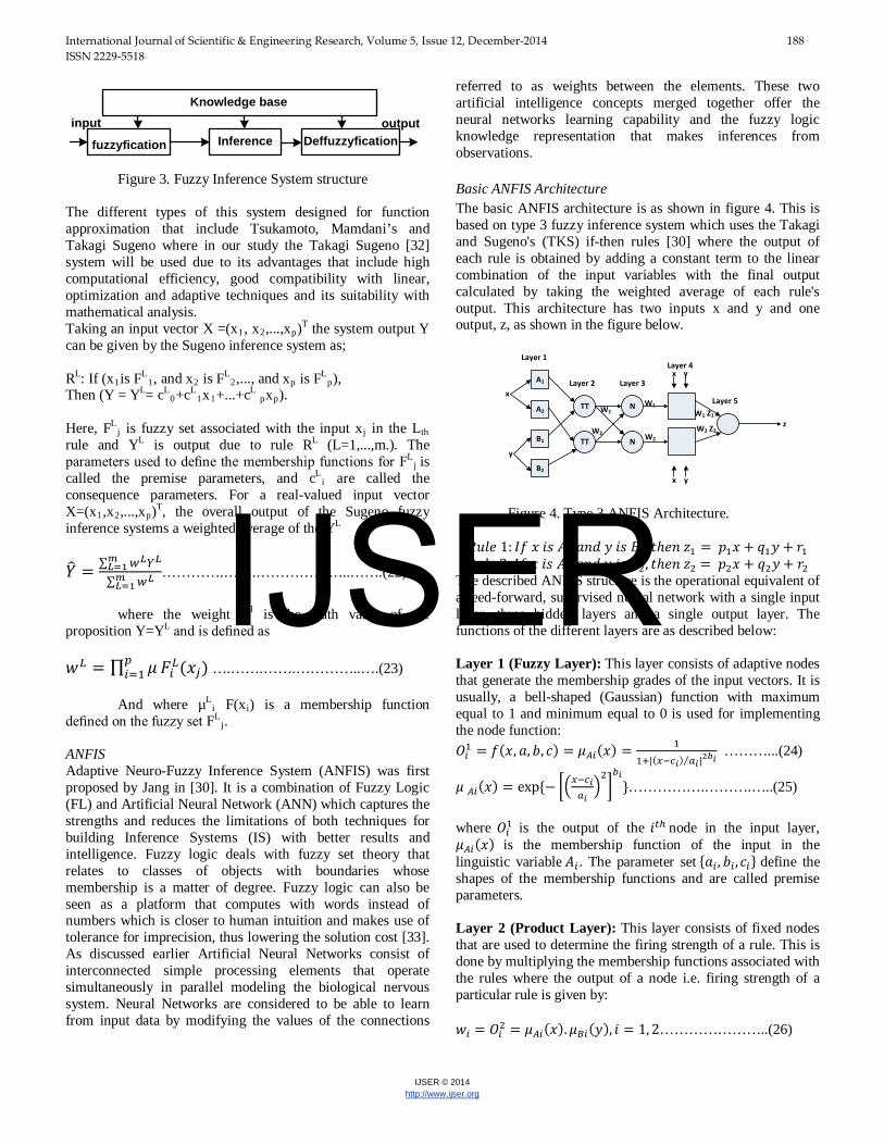
referred to as weights between the elements. These two artificial intelligence concepts merged together offer the neural networks learning capability and the fuzzy logic knowledge representation that makes inferences from observations. Basic ANFIS Architecture The basic ANFIS architecture is as shown in figure 4. This is based on type 3 fuzzy inference system which uses the Takagi and Sugeno's (TKS) if-then rules [30] where the output of each rule is obtained by adding a constant term to the linear combination of the input variables with the final output calculated by taking the weighted average of each rule's output. This architecture has two inputs x and y and one output, z, as shown in the figure below.

A1

A2

B1

B2

TT

TT

N

N

Layer 1

Layer 2 Layer 3

Layer 4

Layer 5

y

x

W1

W2z

x y

x y

W1 Z1

W2 Z2

W1

W2

Figure 4. Type 3 ANFIS Architecture.

𝑅𝑢𝑙𝑒 1: 𝐼𝑓 𝑥 𝑖𝑠 𝐴1 𝑎𝑛𝑑 𝑦 𝑖𝑠 𝐵1 , 𝑡ℎ𝑒𝑛 𝑧1 = 𝑝1𝑥 + 𝑞1𝑦 + 𝑟1 𝑅𝑢𝑙𝑒 2: 𝐼𝑓 𝑥 𝑖𝑠 𝐴2 𝑎𝑛𝑑 𝑦 𝑖𝑠 𝐵2, 𝑡ℎ𝑒𝑛 𝑧2 = 𝑝2𝑥 + 𝑞2𝑦+ 𝑟2

The described ANFIS structure is the operational equivalent of a feed-forward, supervised neural network with a single input layer, three hidden layers and a single output layer. The functions of the different layers are as described below:

Layer 1 (Fuzzy Layer): This layer consists of adaptive nodes that generate the membership grades of the input vectors. It is usually, a bell-shaped (Gaussian) function with maximum equal to 1 and minimum equal to 0 is used for implementing the node function: 𝑂𝑖1 = 𝑓(𝑥, 𝑎,𝑏, 𝑐) = 𝜇𝐴𝑖(𝑥) = 1

1+|(𝑥−𝑐𝑖) 𝑎𝑖|⁄ 2𝑏𝑖 ………...(24)

𝜇 𝐴𝑖(𝑥) = exp {− ��𝑥−𝑐𝑖𝑎𝑖�2�𝑏𝑖

}…………….……….…..(25) where 𝑂𝑖1 is the output of the 𝑖𝑡ℎ node in the input layer, 𝜇𝐴𝑖(𝑥) is the membership function of the input in the linguistic variable 𝐴𝑖. The parameter set {𝑎𝑖 , 𝑏𝑖 ,𝑐𝑖} define the shapes of the membership functions and are called premise parameters. Layer 2 (Product Layer): This layer consists of fixed nodes that are used to determine the firing strength of a rule. This is done by multiplying the membership functions associated with the rules where the output of a node i.e. firing strength of a particular rule is given by: 𝑤𝑖 = 𝑂𝑖2 = 𝜇𝐴𝑖(𝑥).𝜇𝐵𝑖(𝑦), 𝑖 = 1, 2…………………..(26)

IJSER




any other T-norm operator that implements the fuzzy AND operation can be applied in this layer. Layer 3 (Normalized Layer): This layer has fixed nodes that are used to determine the ratio of the ith rule's firing strength to that of the total of all firing strengths: 𝑤� = 𝑂𝑖3 = 𝑤𝑖

𝑤1+𝑤2 , 𝑖 = 1, ..………………….………..(27)

The outputs of this layer are usually known as normalized firing strengths. Layer 4 (Defuzzify Layer): This is an adaptive layer that computes the contribution of each rule to the overall output. The nodes have the following function. 𝑤𝚤��𝑧𝑖 = 𝑂𝑖4 = 𝑤𝚤��(𝑝𝑖𝑥 + 𝑞𝑖𝑦 + 𝑟𝑖)………….………....(28) It is called a defuzzification layer and provides output values resulting from the inference of rules. The parameters in this layer {𝑝𝑖 , 𝑞𝑖 , 𝑟𝑖} are referred to as consequent parameters. Layer 5 (Total Output Layer): This layer consists of a single fixed node that computes the overall output as the summation of contribution from each rule: ∑ 𝑤𝚤��𝑧𝑖𝑖 = 𝑂𝑖5 = ∑ 𝑤𝑖𝑧𝑖

∑ 𝑧𝑖𝑖𝑖 ……………………….……..(29)

B. LEARNING ALGORITHMS The development of the ANFIS concept, has seen the proposal of several learning methods to facilitate the process of obtaining optimal set of rules. They include a merge between Min-Max and ANFIS proposed by Mascioli et al and nonlinear least square by Lavenberg-Marquardt [32]. Four methods used to update the ANFIS structure parameters introduced by Jang [30] are as given below according to their level of computation complexities:

1. Gradient descent (GD) only- used to update all the parameters.

2. Gradient descent only and one pass of least square estimator (LSE)- the gradient descent takes over to update all parameters after the LSE is first applied only once at the beginning to obtain the initial values of the consequent parameters.

3. Gradient descent only and LSE- this is a hybrid learning.

4. Sequential LSE-updates all the parameters using extended Kalman filter.

All these methods have limitations of high complexity and slow converge. In this research we will use, particle swarm optimization (PSO), a method which has less complexity and fast convergence [32].

C. PARTICLE SWARM OPTIMIZATION (PSO) Particle Swarm Optimization is a global optimization technique developed by Eberhart and Kennedy in 1995 [31],

where the underlying motivation of its algorithm was the social behavior observable in nature, such as flocks of birds and schools of fish in order to model swarms of particles moving towards the most promising regions of the search space. It exhibits good performance in finding solutions to static optimization problems where it is considered to be better than other algorithms like Genetic Algorithm [34]. Apart from this it also exploits a population of individuals to synchronously probe promising regions of the search space. In this case, the population is referred to as a swarm and the individuals (i.e. the search points) to as particles. The consideration here is that each particle in the swarm represents a candidate solution to the optimization problem. For a PSO system, every particle moves with an adjustable velocity through the search space, where it adjusts its position in the search space according to its own experience and that of neighboring particles. After this it retains a memory of the best position it ever encountered. A particle therefore makes use of the best position encountered by itself and the best position of neighbors to position itself towards the global minimum. This therefore results to particles “flying” towards the global minimum, while still searching a wide area around the best solution [32]. Each particle’s performance (i.e. the “closeness” of a particle to the global minimum) is measured according to a predefined fitness function which is related to the problem being solved. For our case, a particle represents the weight vector of NNs, including biases. The total number of weights and biases give the dimension of the search space [33].

The iterative approach of PSO can be described as in the following steps:

• Step 1: Initialize a population size, positions and velocities of agents, and the number of weights and biases.

• Step 2: The current best fitness achieved by particle p is set as pbest. The pbest with best value is set as gbest and this value is stored.

• Step 3: Evaluate the desired optimization fitness function 𝑓𝑝 for each particle as the Mean Square Error (MSE) over a given data set.

• Step 4: Compare the evaluated fitness value 𝑓𝑝 of each particle with its pbest value. If 𝑓𝑝< pbest then pbest = 𝑓𝑝 and bestxp= 𝑥𝑝 , 𝑥𝑝 is the current coordinates of particle p, and bestxp is the coordinates corresponding to particle p’s best fitness so far.

• Step 5: The objective function value is calculated for new positions of each particle. If a better position is achieved by an agent, pbest value is replaced by the current value. As in Step 1, gbest value is selected among pbest values. If the new gbest value is better than previous gbest value, the gbest value is replaced by the current gbest value and this value is stored. If 𝑓𝑝< gbest then gbest = p, where gbest is the particle having the overall best fitness over all particles in the swarm.

IJSER




• Step 6: Change the velocity and location of the particle according to Equations 27 and 28, respectively.

• Step 7: Fly each particle p according to Equation 26. • Step 8: If the maximum number of predetermined

iterations (epochs) is exceeded, then stop; otherwise Loop to step 3 until convergence. 𝑉𝑖 = 𝑤𝑉𝑖−1 + 𝑎𝑐𝑐 ∗ 𝑟𝑎𝑛𝑑() ∗ �𝑏𝑒𝑠𝑡𝑥𝑝 − 𝑥𝑝�

+𝑎𝑐𝑐 ∗ 𝑟𝑎𝑛𝑑() ∗ �𝑏𝑒𝑠𝑡𝑥𝑔𝑏𝑒𝑠𝑡 − 𝑥𝑝�….(30)

Where acc is the acceleration constant that controls how far particles fly from one another, and rand returns a uniform random number between 0 and 1.

𝑥𝑝 = 𝑥𝑝𝑝 + 𝑉𝑖……………………..…….(31)

𝑉𝑖 is the current velocity, 𝑉𝑖−1 is the previous velocity, 𝑥𝑝 is the present location of the particle, 𝑥𝑝𝑝 is the previous location of the particle, and i is the particle index. In step 5 the coordinates best 𝑥𝑝 and bestxgbest are used to pull the particles towards the global minimum [32].

D. EVALUATION CRITERIA The performance of the proposed approach will be evaluated by measuring the estimation accuracy. The estimation accuracy can be defined as the difference between the actual and estimated values. The first typical fitting criterion (MSE) is defined as in Equation 28: 𝑀𝑆𝐸 = 1

𝑁∑ (𝑦𝑖 − 𝑦𝚤�)2𝑁𝑖=1 ……………………………..(32)

where N is the total number of data, y is actual target value, and 𝑦� its estimated target value. The experiments will be implemented many times to ensure that MSE converges to a minimum value. The initial values for weights will randomly be assigned within the range [-1; 1]. The training accuracy is expressed in terms of the mean absolute error, standard deviation (SD) and root mean squared error (RMSE). The absolute mean error (ME) is expressed as 𝑒𝑖 = |𝑃𝑚𝑒𝑎𝑠𝑢𝑟𝑒𝑑 − 𝑃𝑠𝑖𝑚𝑢𝑙𝑎𝑡𝑒𝑑|,

�̅� = 1𝑁∑ 𝑒𝑖𝑁𝑖=1 ,……………………………………(33)

where terms measured and simulated denote received signal strength that are obtained by measurement and simulated by ANFIS, while N is total number of samples. Standard deviation is given by

𝜎 = � 1𝑁−1

(𝑒𝑖 − �̅�)2 ………………………….(34)

The root mean squared error (RMSE) is calculated according to the expression

𝑅𝑀𝑆𝐸 = √𝜎2 + �̅�2…………………………………(35)

E. IDENTIFY BUILDINGS We will survey 4 categories of buildings for each category taking five buildings Category 1 Buildings with concrete walls and a few glasses Category 2 Buildings with glass walls and a few concrete walls Category 3 Buildings with iron sheet walls (slums) Category 4 Lifts and Tunnels Category 5 Wooden partitions CW Measurements For this clean unused frequency will be identified. Perform the actual CW measurements after identification of the receiver antenna position at different points of one floor, different floors and the surrounding building environment. Vary the transmitter antenna heights as the measurements are done same floor and different floors. Vary different partitions concrete, wood and iron sheets and also their number. Vary the antenna distance from the buildings. In this study, the measurement equipment will consist of a transmitter and a receiver. The narrow band continuous wave (CW) transmitter, which can be tuned to a specific test frequency, will be used together with an antenna. For the purpose of measurement, a narrow band CW channel will be used. This will ensure good frequency isolation and constant signal to avoid interference. The frequency chosen will be in the unused frequency band not used by GSM operators or anyone else.

F. EXPERIMENTAL SETUP TRANSMITTER RECEIVER

Figure 5. Schematic diagram of Bistatic System

G. STATISTICAL ANALYSIS

Analyse the impact of different partitions, their number, antenna positioning, different floors, inside a lift, effect of other surrounding buildings. The main idea of the statistical

IJSER




analyses (using SPSS) will be to understand the radio wave propagation behavior at the measurement frequency.

H. DEVELOPMENT OF AN INDOOR PROPAGATION MODEL

The neuro fuzzy system with the learning capability of neural network and with the advantages of the rule-base fuzzy system can improve the performance significantly and can provide a mechanism to incorporate past observations into the classification process. In neural network the training essentially builds the system. However, using a neuro fuzzy scheme, the system is built by fuzzy logic definitions and is then refined using neural network training algorithms. Some advantages of ANFIS are: • Refines fuzzy if-then rules to describe the behaviour of a

complex system. • It uses membership functions and desired dataset to

approximate. • Greater choice of membership functions to use. • Very fast convergence time. • Minimized errors. As indicated above ANFIS will be used to develop the indoor propagation model with PSO training.

I. SIMULATION AND TESTING THE MODEL The model will be simulated using MATLAB and the test done on Atoll or IB-wave.

J. COMPARISON OF THE MODEL WITH RBF-NN-

PSO TRAINED MODEL. The evaluation measurements will be done on similar buildings to compare the accuracy of the developed model as well as compare its accuracy with radial basis function (RBF) neural network model trained with particle swarm optimization (PSO) algorithm which according to [35] has results represented in Table 2 and Figure 6.

Table 2: Results for RBF-PSO trained model Absolute

mean error [dB]

Standard deviation [dB]

RMS error [dB]

RBF-PSO 1.847 1.270 2.245

Figure 6: Simulated results obtained by RBF-PSO training algorithm

K. EXPECTED RESULTS

The predictions from the algorithm based on PSO trained ANFIS, and the predictions from radial basis function (RBF) neural network model will be compared with the error criterion expressed in equations (28)-(31). According to the indicated error criterion, the errors obtained from our algorithm will be expected to be less than the errors obtained from the other Models such as in terms MSE, RMSE, SD and ME. Another important expectation is that the proposed model will result to faster convergence that is less computing time. This is because of its environmental adaptation that allows it to learn from a changing environment and parallel structure that allows it to achieve high computation speed.

IV. CONLUSION A review of existing data has identified a need to more closely examine the indoor radiowave propagation prediction. This paper outlines a proposed study to critically assess current limitations underlying radiowave propagation prediction modeling and research and postulates potential issues and implications for this work. Expected outcome of this study is a more efficient and accurate model for predicting outdoor to indoor radiowave propagation.

REFERENCES: [1] H. Hashemi, "The indoor radio propagation channel",

Proc. IEEE, vol. 81, no. 7, pp.943 - 968 , 1993. [2] Popescu, I.; Nikitopoulos, D.; Constantinou, P. &

Nafornita, I. (2006), “Comparison of ANN based models for path loss prediction in indoor environments,” Proceedings of 64th IEEE Vehicular Technology Conference (VTC-2006 Fall), pp. 1-5, Montreal, Sep. 2006, doi:10.1109/VTCF.2006.43

[3] Y. Lu, J. Zhang, X. Gao, P. Zhang, and Y. Wu, "Outdoor-Indoor Propagation Characteristics of Peer-to-Peer

IJSER




System at 5.25 GHz," Vehicular Technology Conference (VTC-2007 Fall), Baltimore, 2007.

[4] Basri, A.A.; Ghasemi, A.; Sydor, J.; “Experimental Evaluation of Outdoor-to-Indoor MIMO Systems with a Multi-Antenna Handset,” Vehicular Technology Conference (VTC Spring), 2011 IEEE 73rd

[5] A. Valcarce and J. Zhang, "Empirical Indoor-to-Outdoor Propagation Model for Residential Areas at 0.9-3.5 GHz, " IEEE Antennas and Wireless Propagation Letters, vol. 9, pp. 682-685, 2010.

[6] C. Oestges, N. Czink, B. Bandemer , P. Castiglione , F. Kaltenberger and A. J. Paulraj "Experimental characterization and modeling of outdoor-to-indoor and indoor-to-indoor distributed channels", IEEE Trans. Veh. Technol., vol. 59, no. 5, pp.2253 - 2265, 2010.

[7] S. Reynaud, M. Mouhamadou, K. Fakih, O. Akhdar, C. Decroze, D. Carsenat, E. Douzon, and T. Monediere, "Outdoor to Indoor Channel Characterization by Simulations and Measurements for OptimisingWiMAX Relay Network Deployment," in IEEE 61st Vehicular Technology Conference VTC-Spring, April 2009.

[8] H. Okamoto, et.al, "Outdoor-to-Indoor Propagation Loss Prediction in 800-MHz to 8-GHz Band for Urban Area," to be appeared in IEEE Trans. on Vehicular Technology.

[9] B. Coppin, “Artificial Intelligence Illuminated,” Sudbury: Jones and Bartlett Publishers, 2004.

[10] M. Reardon, “Cisco predicts wireless data explosion,” Press release, 9th Feb 2010, online available.

[11] V. Chandrasekhar and J. Andrew s, “Femtocell networks: A survey,” IEEE Commun. Mag., vol. 46, no. 9, pp. 59–67, Sep. 2008.

[12] M. Ismail, T. L. Doumi, and J. G. Gardiner, “Teletraffic performance of dynamic cell sectoring for mobile radio system,” ICCS Conference Proceedings, vol. 3, pp. 1090–1094, 14-18 Nov. 1994.

[13] Presentations by ABI Research, Picochip, Airvana, IP access, Gartner, TelefonicaEspana, 2nd Intl. Conf. Home Access Points and Femtocells; available online at:http://www. avrenevents. com/dallas fem to 2007/ purchase presentations. htm.

[14] J. Cullen, “Radioframe presentation,” in Femtocell Europe, London, UK, June. 2008.

[15] TalhaZahir, Kamran Arshad, Atsushi Nakata, and Klaus Moessner, “Interference Management in Femtocells,” Communications Surveys & Tutorials, IEEE 2012.

[16] Valcarce, A. ; de la Roche, G. ; Nagy, L. ; Wagen, J.-F. ; Gorce, J.-M.; “A new trend in propagation Prediction,” Vehicular Technology Magazine, IEEE.

[17] Dagefu, F.T.; Sarabandi, K.; “Simulation and Measurement of Near-Ground Wave Propagation for Indoor Scenarios,” Antennas and Propagation Society International Symposium (APSURSI), 2010 IEEE.

[18] Phillips, C.; Sicker, D.; Grunwald, D.; “A Survey of Wireless Path Loss Prediction and Coverage Mapping Methods,”Communications Surveys & Tutorials, IEEE.

[19] Klepal, M. “Novel Approach to Indoor Electromagnetic Wave Propagation Modelling,” Ph.D. Thesis, Czech Technical University, Prague, 2003; pp. 4-8.

[20] T. M. Schaefer and W. Wiesbeck "Simulation of radiowave propagation in hospitals based on FDTD and ray-optical methods", IEEE Trans. Antennas Propag., vol. 53, p.2381, 2005.

[21] Gentile, M.; Monorchio, A.; Manara, G.; “Electromagnetic Propagation into Not Deterministic Sceneries by Using an Efficient Ray Tracing Simulator,” Antennas and Propagation Society International Symposium 2006, IEEE.

[22] SUBRT, L., PECHAC, P. “Semi-deterministic propagation modelfor subterranean galleries and tunnels,” IEEE Transactions on Antennas and Propagation, Accepted May, 2010.

[23] Y. Corre, Y. Lostanlen, "3D urban EM wave propagation model for radio network planning and optimization over large areas," IEEE Transactions on Vehicular Technology, in press.

[24] De la Roche, G.; Valcarce, A.; Jie Zhang; “Hybrid Model for Indoor-to-Outdoor Femtocell Radio Coverage Prediction,” Vehicular Technology Conference (VTC Spring), 2011 IEEE 73rd.

[25] Andrade, C. B. and Hoeful, R. P. F. “IEEE 802.11WLANs: A Comparison on Indoor CoverageModels”. In Proceedings of the 23rd CanadianConference on Electrical and Computer Engineering, 2010.

[26] D. Xu, J. Zhang, X. Gao, P. Zhang, and Y. Wu, "Indoor Office Propagation Measurements and Path Loss Models at 5.25 GHz,” IEEE Veh. Technol. Conf. (VTC), pp. 844-848, Oct. 2007.

[27] Abhayawardhana, V.S., Wassell, I.J., Crosby, D., Sellars, M.P., and Brown, M.G., "Comparison of Empirical Propagation Path Loss Models for Fixed Wireless Access Systems", VTC 2005.

[28] Caleb Phillips, Douglas Sicker and Dirk Grunwal, “A Survey of Wireless Path Loss Prediction and Coverage Mapping Methods,” IEEE Communications Surveys & Tutorials, Accepted For Publication, Feb. 2012.

[29] Erik Östlin, Hans-Jürg en Zepernick a nd Hajime S uzuki, “Macrocell Path-Loss Prediction Using Artificial Neural Networks,” IEEE Transactions on Vehicular Technology, Vol. 59, No. 6, July 2010, pg. 2735-2746.

[30] J. S. Jang, “ANFIS: Adaptive-network-based fuzzy inference system”, IEEE Trans. Syst., Man, Cybern., vol. 23, pp.665 -685 1993.

[31] J. Kennedy and R. C. Eberhart, “Particle swarm optimization”, Proc. IEEE Int. Conf. Neural Networks, pp.1942 -1948 1995.

[32] V. S. Ghomsheh, M. A. Shoorehdeli and M. Teshnehlab, “Training ANFIS structure with modified PSO algorithm”, Proc. 15th Mediterranean Conf. Control Automation, 2007.

IJSER


http://ieeexplore.ieee.org/xpl/mostRecentIssue.jsp?punumber=5954014


http://ieeexplore.ieee.org/xpl/RecentIssue.jsp?punumber=9739

http://ieeexplore.ieee.org/search/searchresult.jsp?searchWithin=Authors:.QT.Valcarce,%20A..QT.&newsearch=partialPref

http://ieeexplore.ieee.org/search/searchresult.jsp?searchWithin=Authors:.QT.%20de%20la%20Roche,%20G..QT.&newsearch=partialPref

http://ieeexplore.ieee.org/search/searchresult.jsp?searchWithin=Authors:.QT.%20Nagy,%20L..QT.&newsearch=partialPref

http://ieeexplore.ieee.org/search/searchresult.jsp?searchWithin=Authors:.QT.%20Wagen,%20J.-F..QT.&newsearch=partialPref

http://ieeexplore.ieee.org/search/searchresult.jsp?searchWithin=Authors:.QT.%20Gorce,%20J.-M..QT.&newsearch=partialPref




http://ieeexplore.ieee.org/search/searchresult.jsp?searchWithin=Authors:.QT.Phillips,%20C..QT.&newsearch=partialPref

http://ieeexplore.ieee.org/search/searchresult.jsp?searchWithin=Authors:.QT.%20Sicker,%20D..QT.&newsearch=partialPref

http://ieeexplore.ieee.org/search/searchresult.jsp?searchWithin=Authors:.QT.%20Grunwald,%20D..QT.&newsearch=partialPref








[33] S. Sumathiand and S. Paneerselvam, “Computational intelligence paradigms: theory & applications using MATLAB”, CRC Press Taylor & Francis Group, 2010.

[34] R. Hassan, B. Cohanim, and O. de Weck, “A comparison of particle swarm optimization and the genetic algorithm,” presented at the AIAA/ASME/ASCE/AHS/ASC 46th Struct., Struct. Dyn. Mater. Conf., Austin, TX, Apr. 2005.

[35] I. Vilovic and N. Burum, “A Comparison of MLP and RBF Neural Networks Architectures for Electromagnetic Field Prediction in Indoor Environments,” Antennas and Propagation (EUCAP), Proceedings of the 5th European Conference, pp. 1719 – 1723, April 2011.

IJSER


Documents

The Application of ANFIS-PSO trained in Signal Propagation ... · communication presently and in the future is expected to originate from indoor ... in inferior call quality ... as