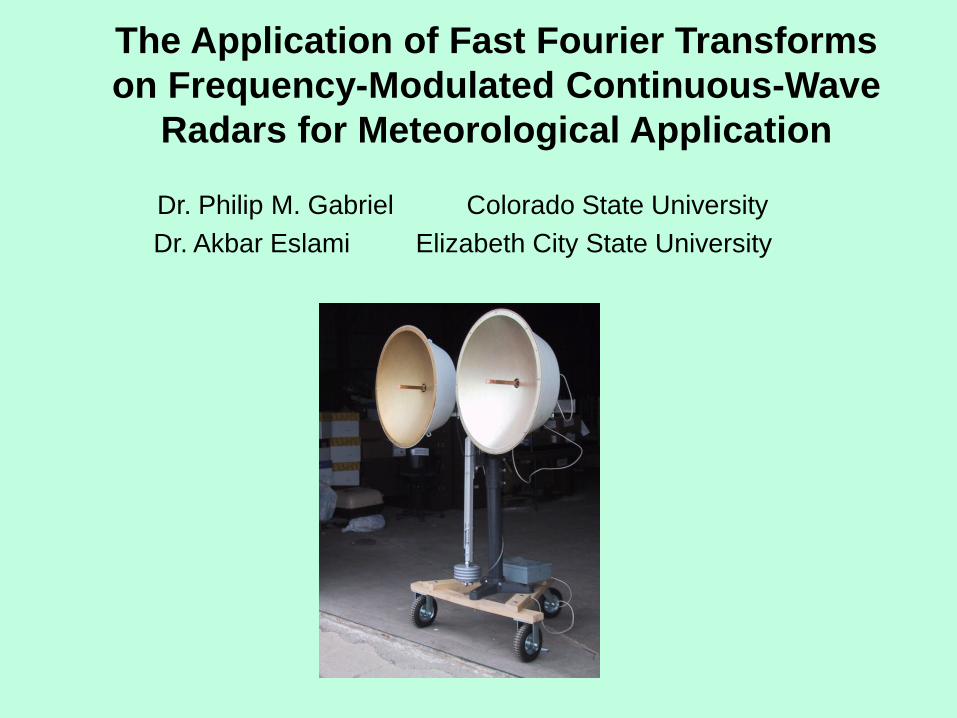
The Application of Fast Fourier Transforms on Frequency-Modulated Continuous-Wave

Radars for Meteorological Application

Dr. Philip M. Gabriel Colorado State University Dr. Akbar Eslami Elizabeth City State University

A little bit of background… • This presentation is based on our design,

construction, simulation, and experience using a Frequency-Modulated Continuous-Wave (FM-CW) radar.

• This instrument performs detection and ranging in the frequency domain as opposed to the time domain wherein conventional radars operate.

• This type of radar is not new. Much credit demonstrating the use of FM-CW in remote sensing with applications to atmospheric science is credited to Richard Strauch (1974).

• This radar is design at Colorado State University to detect precipitation (rain and snow) at high spatial resolution over relatively short ranges (e.g. 33 km).

background

• FM-CW radar can be used to measure exact height of landing aircraft. The advantage of using these radar signals is that the object target velocity and range can be quickly calculated using Fast Fourier Transforms (FFT).

• FFT is a commonly used signal-processing technique that converts time-varying signals to their frequency component.

Application Domain of FM-CW Radars

• Radio altimeters in the avionics of most military and civilian aircraft. Also used for space vehicles during landing.

• Proximity fuses for artillery shells and missiles.

• Systems for detecting mobile targets. • Measuring small and very small ranges

to a target with minimal range, comparable to wavelength (e.g. levels of liquid, paste or powder-like products in closed tanks).

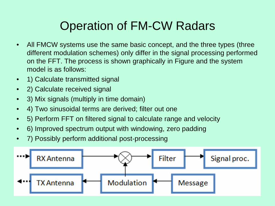
Operation of FM-CW Radars • All FMCW systems use the same basic concept, and the three types (three

different modulation schemes) only differ in the signal processing performed on the FFT. The process is shown graphically in Figure and the system model is as follows:

• 1) Calculate transmitted signal • 2) Calculate received signal • 3) Mix signals (multiply in time domain) • 4) Two sinusoidal terms are derived; filter out one • 5) Perform FFT on filtered signal to calculate range and velocity • 6) Improved spectrum output with windowing, zero padding • 7) Possibly perform additional post-processing

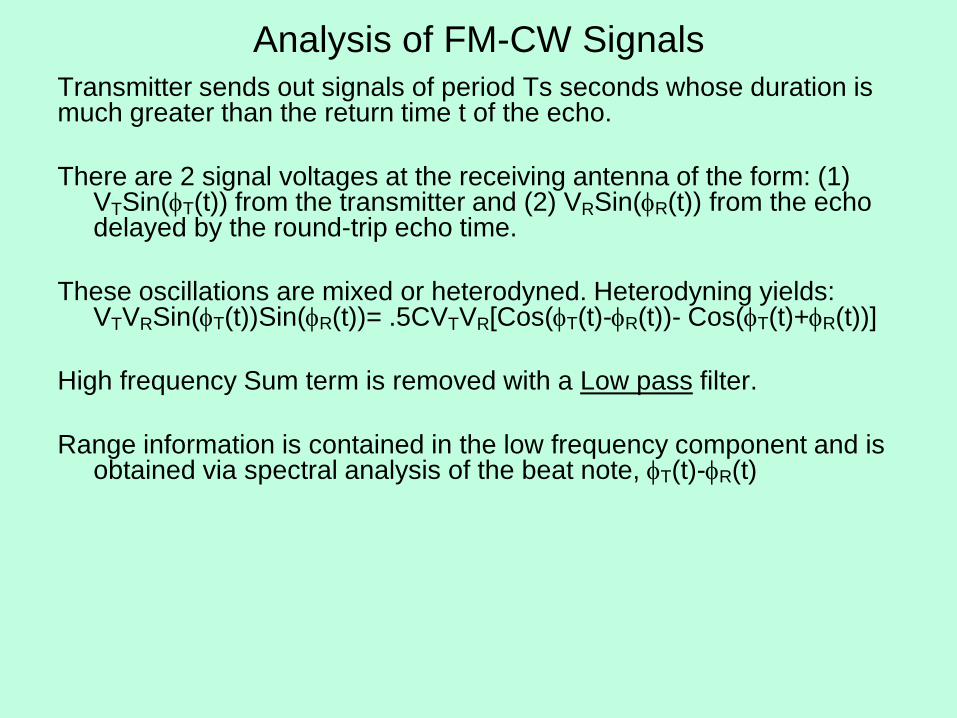
Analysis of FM-CW Signals Transmitter sends out signals of period Ts seconds whose duration is much greater than the return time t of the echo. There are 2 signal voltages at the receiving antenna of the form: (1)

VTSin(φT(t)) from the transmitter and (2) VRSin(φR(t)) from the echo delayed by the round-trip echo time.

These oscillations are mixed or heterodyned. Heterodyning yields:

VTVRSin(φT(t))Sin(φR(t))= .5CVTVR[Cos(φT(t)-φR(t))- Cos(φT(t)+φR(t))] High frequency Sum term is removed with a Low pass filter. Range information is contained in the low frequency component and is

obtained via spectral analysis of the beat note, φT(t)-φR(t)

discretizing and sampling of signals

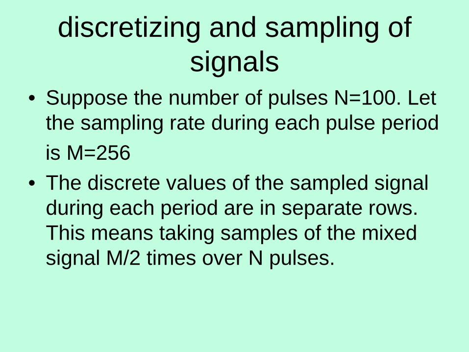
• Suppose the number of pulses N=100. Let the sampling rate during each pulse period

is M=256 • The discrete values of the sampled signal

during each period are in separate rows. This means taking samples of the mixed signal M/2 times over N pulses.

discretizing and sampling of signals

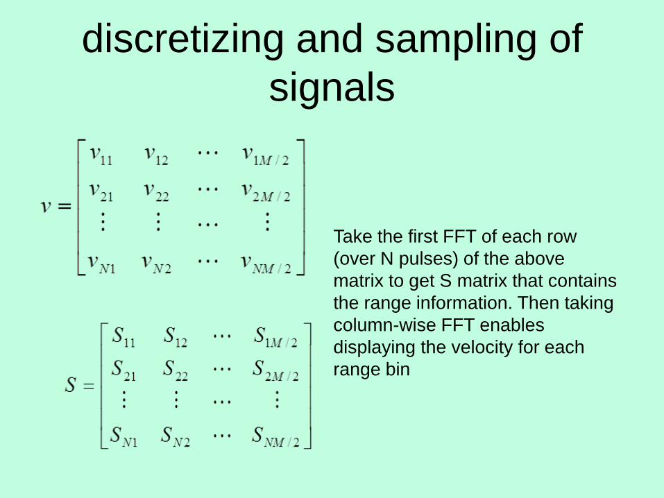
Take the first FFT of each row (over N pulses) of the above matrix to get S matrix that contains the range information. Then taking column-wise FFT enables displaying the velocity for each range bin

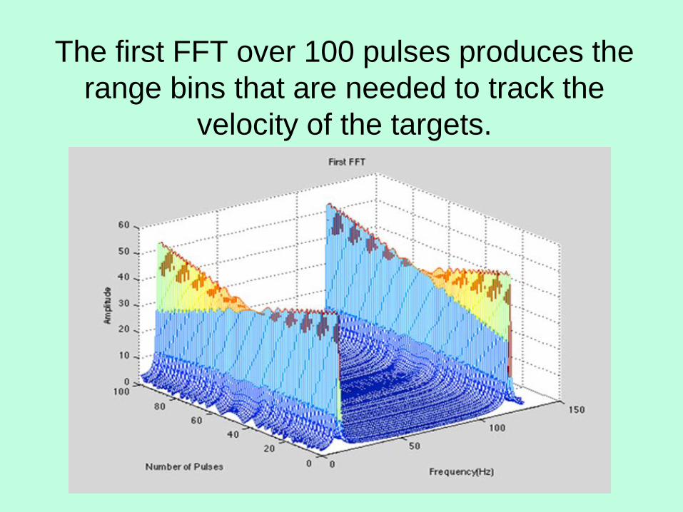
The first FFT over 100 pulses produces the range bins that are needed to track the

velocity of the targets.

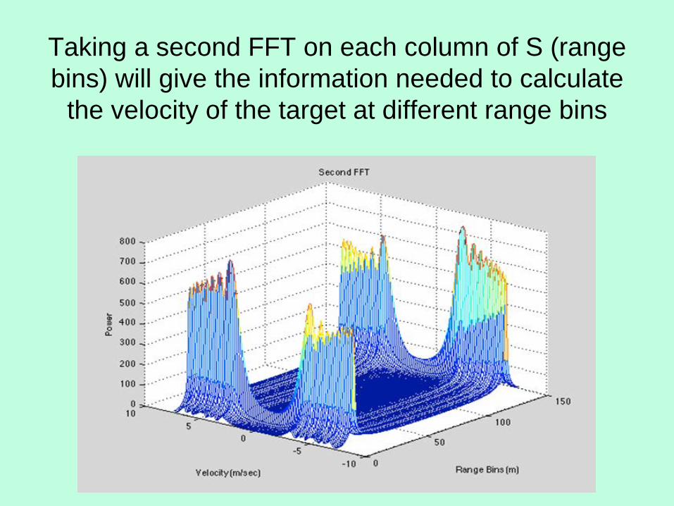
Taking a second FFT on each column of S (range bins) will give the information needed to calculate

the velocity of the target at different range bins

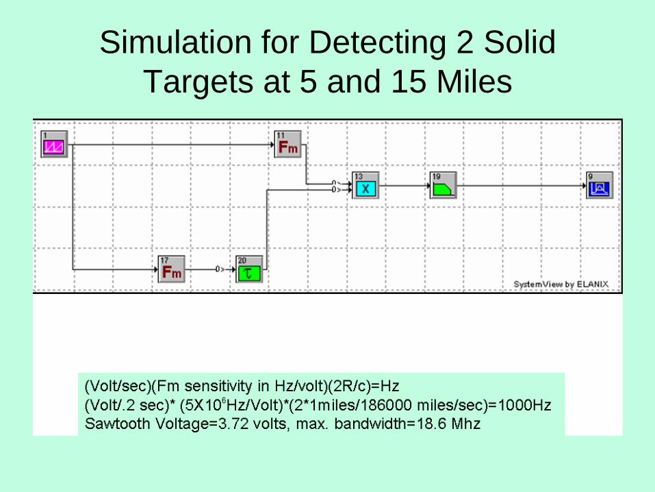
Simulation for Detecting 2 Solid Targets at 5 and 15 Miles

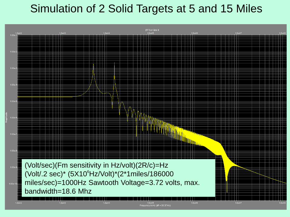
Simulation of 2 Solid Targets at 5 and 15 Miles

(Volt/sec)(Fm sensitivity in Hz/volt)(2R/c)=Hz (Volt/.2 sec)* (5X106Hz/Volt)*(2*1miles/186000 miles/sec)=1000Hz Sawtooth Voltage=3.72 volts, max. bandwidth=18.6 Mhz

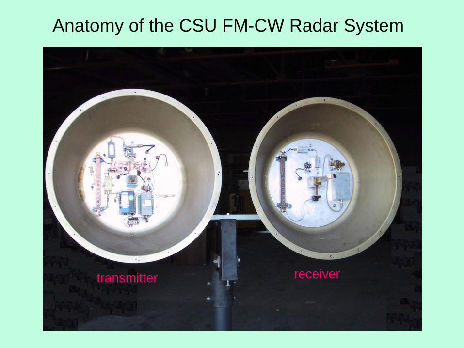
Anatomy of the CSU FM-CW Radar System

transmitter receiver

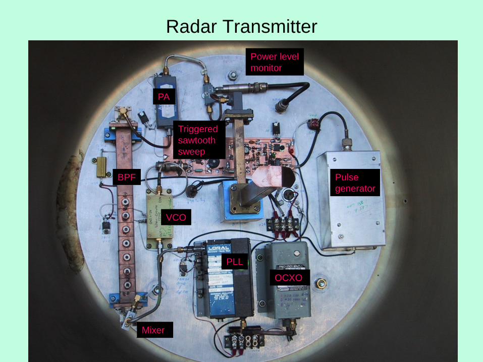
Radar Transmitter

Pulse generator

OCXO

PLL

Mixer

VCO

BPF

PA

Triggered sawtooth sweep

Power level monitor

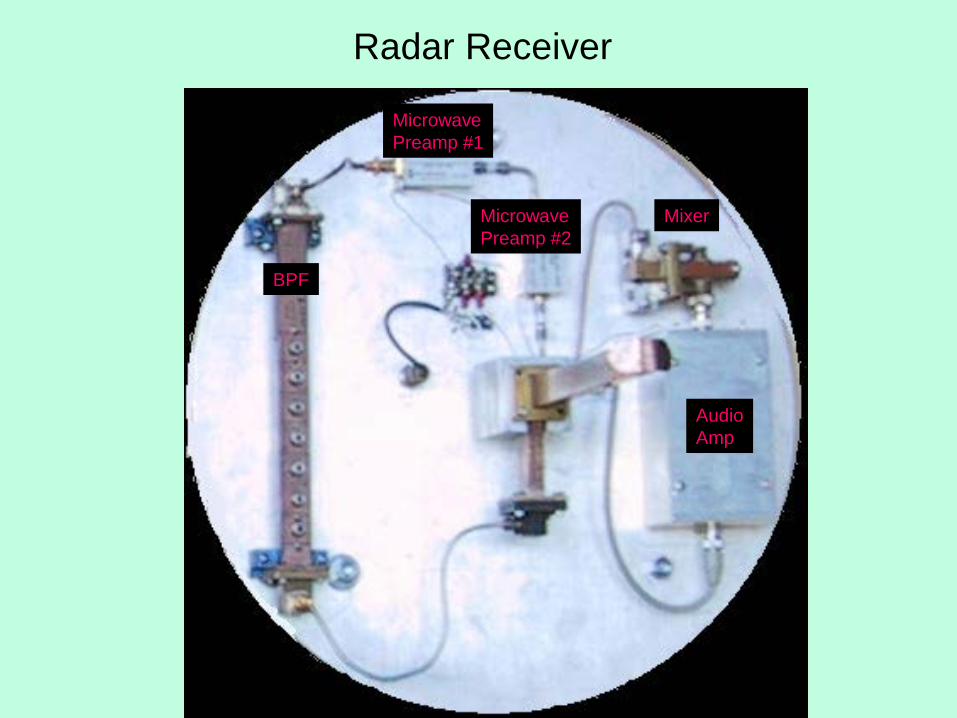
Radar Receiver

BPF

Microwave Preamp #1

Microwave Preamp #2

Mixer

Audio Amp

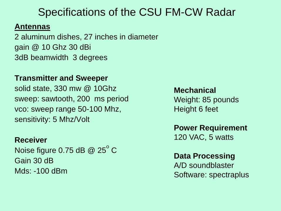
Specifications of the CSU FM-CW Radar Antennas 2 aluminum dishes, 27 inches in diameter gain @ 10 Ghz 30 dBi 3dB beamwidth 3 degrees Transmitter and Sweeper solid state, 330 mw @ 10Ghz sweep: sawtooth, 200 ms period vco: sweep range 50-100 Mhz, sensitivity: 5 Mhz/Volt Receiver Noise figure 0.75 dB @ 25o C Gain 30 dB Mds: -100 dBm

Mechanical Weight: 85 pounds Height 6 feet Power Requirement 120 VAC, 5 watts Data Processing A/D soundblaster Software: spectraplus

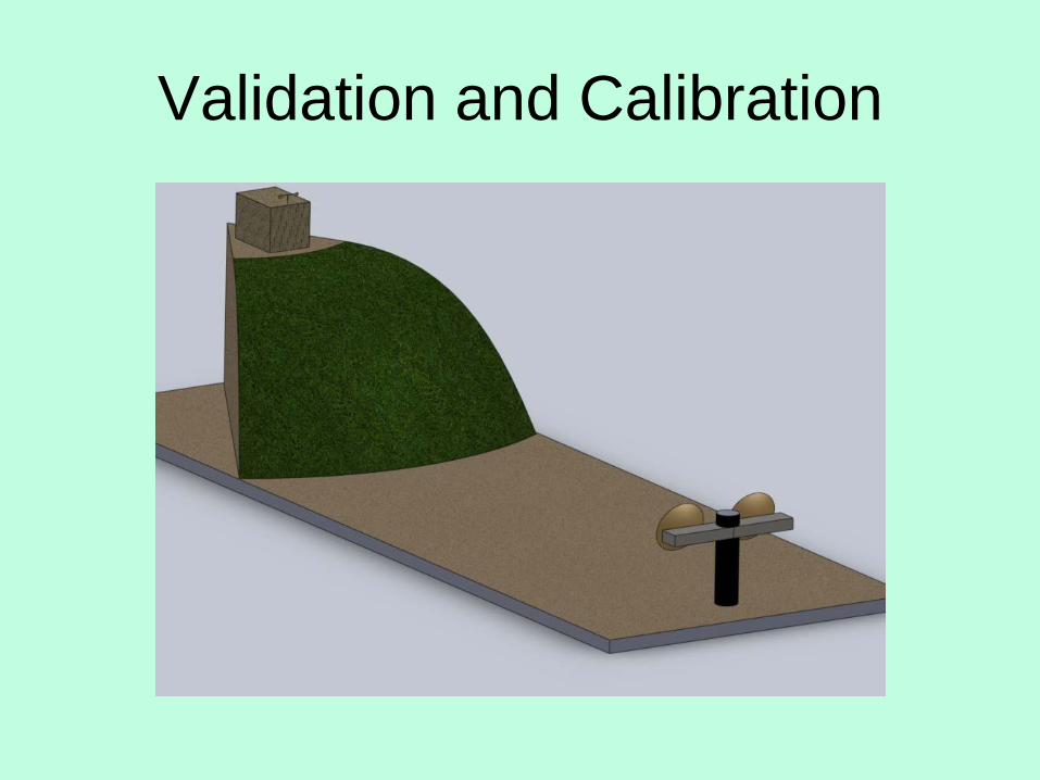
Validation and Calibration

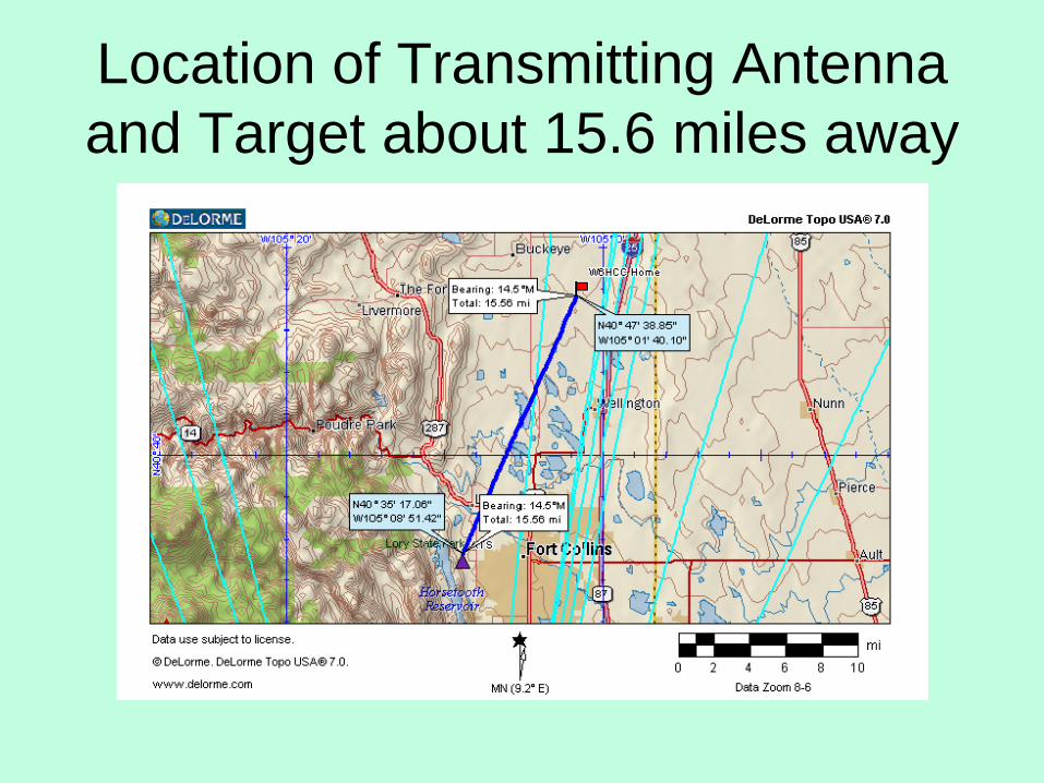
Location of Transmitting Antenna and Target about 15.6 miles away

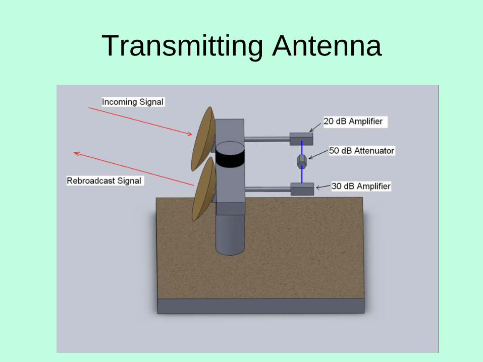
Transmitting Antenna

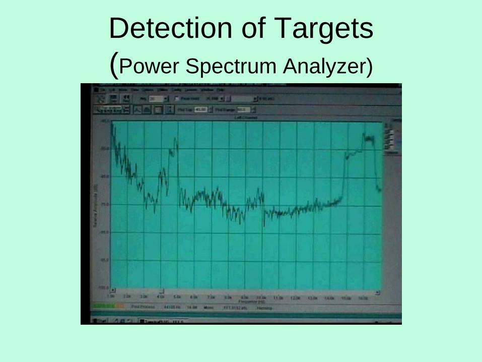
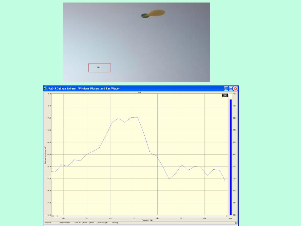
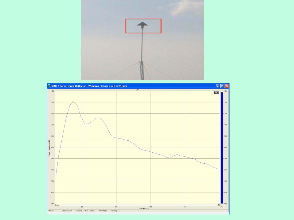
Detection of Targets (Power Spectrum Analyzer)

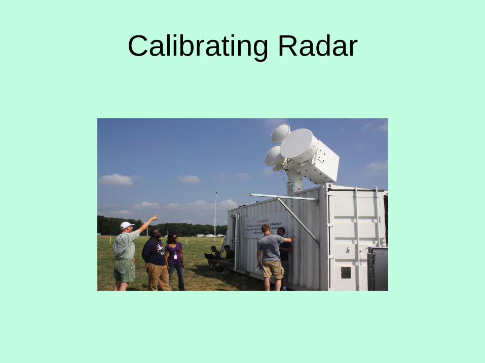
Calibrating Radar

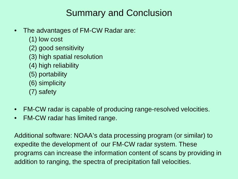
Summary and Conclusion

• The advantages of FM-CW Radar are: (1) low cost (2) good sensitivity (3) high spatial resolution (4) high reliability (5) portability (6) simplicity (7) safety • FM-CW radar is capable of producing range-resolved velocities. • FM-CW radar has limited range.

Additional software: NOAA’s data processing program (or similar) to expedite the development of our FM-CW radar system. These programs can increase the information content of scans by providing in addition to ranging, the spectra of precipitation fall velocities.