THE APPLICATION OF MULTIRATE TECHNIQUES FOR SYNCHRONIZATION IN FULLY DIGITAL DEMODULATION

by

Wei Han

A thesis submitted in partial fulfillment of the requirement for the degree of Master of Engineering. Examination Committee : Dr. Kimmo Mäkeläinen (Chairman) Dr. Kazi Mohiuddin Ahmed Dr. Jian-Guo Zhang Wei Han Nationality : Chinese Previous degree : B.Eng. (Electronics Engineering) Beijing Polytechnic University Beijing, People’s Republic of China Scholarship donor : Government of Japan

Asian Institute of Technology Bangkok, Thailand

December, 1995

-ii-

ACKNOWLEDGMENTS The author takes this opportunity to express his profound gratitude, most sincere appreciation and utmost thanks to his advisor Dr. Kimmo Mäkeläinen for his excellent guidance, valuable suggestions and continued encouragement during the whole thesis period. Sincere acknowledgment to Dr. Kazi Mohiuddin Ahmed for his valuable comments and suggestions in the completion of the project work. Also thanks to Dr. Jian-Guo Zhang for his kind decision to serve as examination member and profitable encouragement. The author is also indebted to Dr. Steffen Lochman for his helpful suggestions during the proposal period of this thesis. Special thanks to scholarship donor government of Japan for their financial support which enable the author to avail the opportunity to study in AIT. The author conveys his sincere thanks to all his colleagues who in one way or anther helped during this study. Thanks to Dr. Jon Shaw and Mr. Balasubramaniam Sivagurunathan for their generously help. Finally, the author expresses deepest gratitude to his parents for their unwavering love, unbounded sacrifices and continued encouragement during the course of this study.

-iii-

ABSTRACT

This study presents an multirate technique as a timing recovery scheme for digital cellular mobile systems in the digital signal processing environment. π/4-shifted-DQPSK modulation is used according to the North American IS-54 TDMA frame structure. The feasibility of the application of square in-phase and quadrature (SIQ) signal phases as a timing recovery detection signal and their BER performances in fading channels corrupted by CCI and AWGN, are investigated in MATLAB. The phase searching processor is a unit that can extract the appropriate timing instant by comparing the SIQ signal phase with the reference signal phase. The phase adjuster, which is employed to diminish phase distortion caused by fading channel, is used to implement synchronizer design. Its BER performance is measured and compared with the expected performance under various operating conditions, such as two rays Rayleigh fading channel or six bins channel based on the GSM specification, and with interferer from varying power.

-iv-

TABLE OF CONTENTS CHAPTER TITLE PAGE Title Page i Acknowledgments ii Abstract iii Table of Contents iv List of Abbreviations vi I INTRODUCTION 1 1.1 Background of the Study 1 1.2 Problem Statement 2 1.3 Scope of the Thesis 3 II LITERATURE REVIEW 4 2.1 Description of the Digital Cellular Mobile Systems 4 2.1.1 π/4-Shifted-DQPSK Modulation Techniques 5 2.1.2 Cellular Mobile Fading Channel 5 2.2 A General Description of Symbol Synchronization Techniques 8 2.3 The Multirate Techniques 11 III METHODOLOGY 16 3.1 General Description of Synchronization 16 3.2 Simulation Model of π/4-DQPSK Modulation for DCM Systems 17 3.2.1 Transmitter 18 3.2.2 Model of the Receiver 20 3.2.3 Simulation Model of Synchronizer 21 3.2.4 Decimation and Differential Detector 28 3.3 Simulation Set-up 28 IV SIMULATION RESULTS AND DISCUSSION 33 4.1 Introduction 33 4.3 Simulation Results 33 V CONCLUSIONS AND RECOMMENDATIONS 43 5.1 Conclusions 43 5.2 Recommendations for Future Research 44

-v-

REFERENCES 45 APPENDIX A 48 APPENDIX B 51

-vi-

LIST OF ABBREVIATIONS

ACI : Adjacent Channel Interference AWGN : Additive White Gaussian Noise BER : Bit Error Rate BPSK : Binary Phase Shift Keying C/I : The desired average signal power (C) to the average interference signal power (I) ratio CCI : Cochannel Interference DCM : Digital Cellular Mobile DD : Differential Detector DFE : Decision Feedback Equalizer DQPSK : Differential Quadrature Phase Shift Keying DSP : Digital Signal Processing DST : Discrete Sine Transform DFL : Digital Feedback Loop Eb/N0 : The average energy per bit-to-noise power spectrum density FED : Frequency Error Detector FFT : Fast Fourier Transform FIR : Finite Duration Impulse Response FSK : Frequency Shift Keying GMSK : Gaussian Minimum Shift Keying GSM : Global System for Mobile communications HI : Hilly Terrain IF : Intermediate Frequency IIR : Infinite Duration Impulse Response ISI : Intersymbol Interference MS : Mobile Station MSE : Mean Square Error MSK : Minimum Shift Keying NCO : Number Controlled Oscillator PAM : Pulse Amplitude Modulation PDF : Probability Density Function PLL : Phase Lock Loop QAM : Quadrature Amplitude Modulation QPSK : Quadrature Phase Shift Keying RA : Rural Area

-vii-

SIQ : Square in-phase and quadrature SRRC : Square Root Raised Cosine TDMA : Time Division Multiple Access TED : Timing Error Detector TU : Typical Urban VCO : Voltage Controlled Oscillator VLSI : Very Large Scale Integration

-1-

CHAPTER I

INTRODUCTION

1.1 Background of the Study Digital cellular mobile (DCM) communication systems is introduced and become operational in many countries around the world. These “second generation” national and international land mobile and satellite mobile systems requires an increased capacity, that is, DCM systems can support more users per base station per MHz of spectrum. In order to accommodate the 15-20 million or even more users toward the end of this century, new modem techniques will be required. Recently, one attractive modulation scheme has been used in Japanese and North American second generation DCM systems, that is the π/4-shifted Quadrature Phase-Shift Keying (π/4-QPSK) modems, which can be viewed as the superposition of two QPSK signal constellations offset by π/4 relative to each other. The cellular mobile channel is characterized by fading, with large frequency shift due to the Doppler effect, and the Cochannel Interference (CCI). Fading is regarded as multiplicity distortion that modulates the received signal in amplitude and phase. A fading channel can be classified as Gaussian, Rayleigh or Rician channel depend on the ratio of the power in the dominant path to the power of the scattered paths. Synchronization is one fundamental problem in digital communication systems. Generally, in the implementation of digital communication systems, there are some different types of synchronization. The five main types are listed below: 1) Carrier synchronization: It is required for the operation of a phase-coherent demodulator. 2) Symbol (or clock) synchronization: Efficient data detection requires that the receiver know when one data symbol ends and the next one begins. 3) Codeword and node synchronization: The decoder can operate correctly when the recovered symbols can be separated into the proper groups. 4) Frame synchronization: In TDMA scheme, for proper reconstruction of the data in terms of their original time samples, time scale alignment process is needed. 5) Network synchronization: When digital data received from several sources, or processed, and retransmitted to one or more users, the network synchronization should be considered. [GARDNER and LINDSEY (1980)]

-2-

Symbol synchronization or timing recovery is one of the most critical receiver functions in synchronous communication systems. The receiver clock must be continuously adjusted in its frequency and phase. Then optimize the sampling instants of the received data signal and compensate for frequency drifts between the oscillators used in the transmitter and receiver clock circuits. The timing phase for a given system will depend on the overall impulse response and thus on the characteristics of the communication channel. In digital mobile communication systems, the symbol synchronization schemes are severely degraded when the delay spread is large or CCI is present. In fully digital realizations of receiver, the synchronous data signal is available only to use sampled received signal for further processing. Therefore, sampling of the received signal is needed to be introduced. In some circumstances, the sampling can be synchronized to the symbol rate of the incoming signal. In other circumstances, the sampling cannot be synchronized to the incoming signal. To produce the correct sampling instants at the modem output when the sampling clock is not possible to be controlled by timing loop, multirate is the way. The term “multirate” is not a quite new concept, and it has been used as a tool in Digital Signal Processing (DSP) since the digital techniques become more popular and important. In practice, the implementation of multirate is concerned with the digital filter design. In general, the finite duration impulse response (FIR) digital filter has the advantages over the infinite duration impulse response (IIR) digital filter for use as multirate filters. Obviously, it is a DSP operation on the signal itself, not on a local clock or timing wave. Therefore, the significant characteristics of timing recovery by multirate techniques are (i) Fixed local sampling that doesn’t synchronize with the incoming signal. (ii) Without forward or feedback timing control loop for local sampling clock. i.e. the local sampler can be designed independently related to the following digital processing part, and this reduce the complexity of digital to analog feedback loop design and vice versa. As a conclusion, in fully digital demodulation, if the sampling in a digital modem is not synchronized with the data symbols, timing must be adjusted by interpolating or decimating new samples among the original ones. 1.2 Problem Statement The performance of symbol synchronization system depends on the ability of the timing recovery circuit to provide an optimum timing instant. The intersymbol interference (ISI), additive white Gaussian Noise (AWGN) and specific interference related to mobile radio systems such as CCI and Adjacent Channel Interference (ACI) cause the degradation in timing synchronization. The conventional timing recovery, analog or digital, utilize forward or feedback

-3-

loop for sampling clock control. The symbol synchronization can be achieved by using analog methods such as narrow-band filter or Phase-Lock Loop (PLL) and digital or hybrid methods. However, digital realization of receivers is of growing interest as the VLSI techniques become feasible and economy. The applications of high speed sampling rate are commonly used for DSPs today. Therefore, fully digital operations can replace the corresponding analog implementations. The problem is that, usually, to realize a totally digitized performance, the sampling rates have to be unsynchronized with the transmitted signal. Hence it is necessary to interpolate or decimate vicinity samples in order to obtain an appropriate value for symbol instant. Until now the timing recovery scheme for some modulation schemes such as PAM, FSK, MSK, BPSK, QPSK, 8PSK, QAM, etc., had already set up and still need further development. While the π/4-DQPSK which is preferable in second generation DCM system is not a new scheme but needs further investigation. As a result, there are considerable works should be done for π/4-DQPSK timing recovery in mobile radio systems by means of multirate techniques in fully digital demodulator. 1.3 Scope of the Thesis The scope of this study is limited to the following items: 1. Design and implementation of synchronizer and decimator 1.1 decimating filter and data filter 1.2 Timing Recovery algorithm 1.3 Phase adjuster and smoothing filter 2. Simulation model for a π/4-shifted-DQPSK modulation signal 3. Simulation model for cellular mobile channel 3.1 Doppler filter design 3.2 Rayleigh fading channel design 3.3 Additive white Gaussian noise 3.4 Cochannel interference (CCI) 4. Establishing a BER simulation model for the Rayleigh mobile radio channel in MATLAB environment 5. Evaluate the fully digital demodulator performance

-4-

CHAPTER II

LITERATURE REVIEW 2.1 Description of the Digital Cellular Mobile Systems There are several mobile and cellular communications applications that have being developed or finished, such as ADC, GSM, DECT, DCS1800, JDC, APCO-25, etc. The modem techniques recommended and already adopted for them are π/4-QPSK, GMSK, GFSK, and 4PAM-FM as indicated by FEHER (1991). A power efficient digital communications systems may have to be nonlinearly amplified for cost-effective utilization of the available power. However, when a bandlimited linearly modulated carrier with nonconstant envelope undergoes nonlinear amplification, the filter side-lobes are restored and in-phase to quadrature in-band crosstalk is generated. This causes severe adjacent channel and cochannel interference. Constant envelope modulation techniques can be nonlinearly amplified without significant spectral regeneration, and can be differentially or discriminator detected. Recently, linear modulation techniques for nonlinearly amplified systems have been used, and they can simultaneously satisfy the power and the spectral efficiency requirements. Traditionally, digital communications systems use coherent detection, and it performs well in stationary additive white Gaussian noise (AWGN) environments. It also has a theoretical power efficiency advantage in Rayleigh and Rician faded mobile systems. However, their performance may degrade significantly when disturbances such as multipath fading, Doppler shifts and other excessive forms of phase noise are present. An alternative method is differential detection. PSK signal can not be noncoherently detected, since the information resides in the received phase. However, if the information is mapped to the phase differences between successive symbols, then the received signal can be detected differentially by comparing the phase of the current received symbol to the phase of the previous symbol. The advantage of DQPSK is that it can be noncoherently demodulated by differential detection. Various digital modulation techniques for mobile and personal communication systems were described by AGHVAMI (1993). In selecting a suitable modulation scheme for a DCM system, consideration must be given to achieving the following: • High bandwidth efficiency • High power efficiency

-5-

• Low signal-to-cochannel interference power ratio (CCI) • Low out-of-band radiation • Low sensitivity to multipath fading • Constant or near constant envelope • Low cost and ease of implementation To optimize all these features at the same time is not possible as each has its practical limitation and also is related to the others. Hence, a trade-off among all the above features must be adopted. 2.1.1 π/4-Shifted-DQPSK Modulation Techniques π/4-Shifted-QPSK modulation scheme has a number of advantages as list below: (i) Power efficient amplifier can be used without introducing significant spectral regeneration (spectral restoration, regrowth or splatter) of the transmitted carrier. (ii) Extremely low out-of-band radiation can be achieved after nonlinear power efficient amplification without the need for postamplification filtering. (iii) Synchronization can be achieved fast and immunity against fast fading can be provided. These can be achieved by noncoherent (differential or discriminator) detection. (iv) Adaptive equalization or other fading countermeasure techniques to mitigate the effect of excessive radio propagation caused delay spread and of Doppler shift can be implemented. CHENNAKESHU and SAULNIER (1993) investigate π/4-Shifted-DQPSK modulation techniques which is essentially π/4-Shifted-QPSK with differential encoding of the symbol phase. They use a tangent type differential detector with an integrated symbol timing and an algorithm for carrier frequency error estimation. The detector is less sensitive to carrier frequency errors and to amplitude variations in the received signal, relative to the sine-cosine detectors. The estimation of modulation systems can be obtained from the computation of the BER. The BER of π/4-Shifted-DQPSK in a Rayleigh fading and Gaussian noise channel was presented by TJIANG et al, (1993). They derive a new Probability Density Function (pdf) for the phase angle between two Rayleigh vectors perturbed by Gaussian noise, which includes the effects of ISI and noise correlation. 2.1.2 Cellular Mobile Fading Channel

-6-

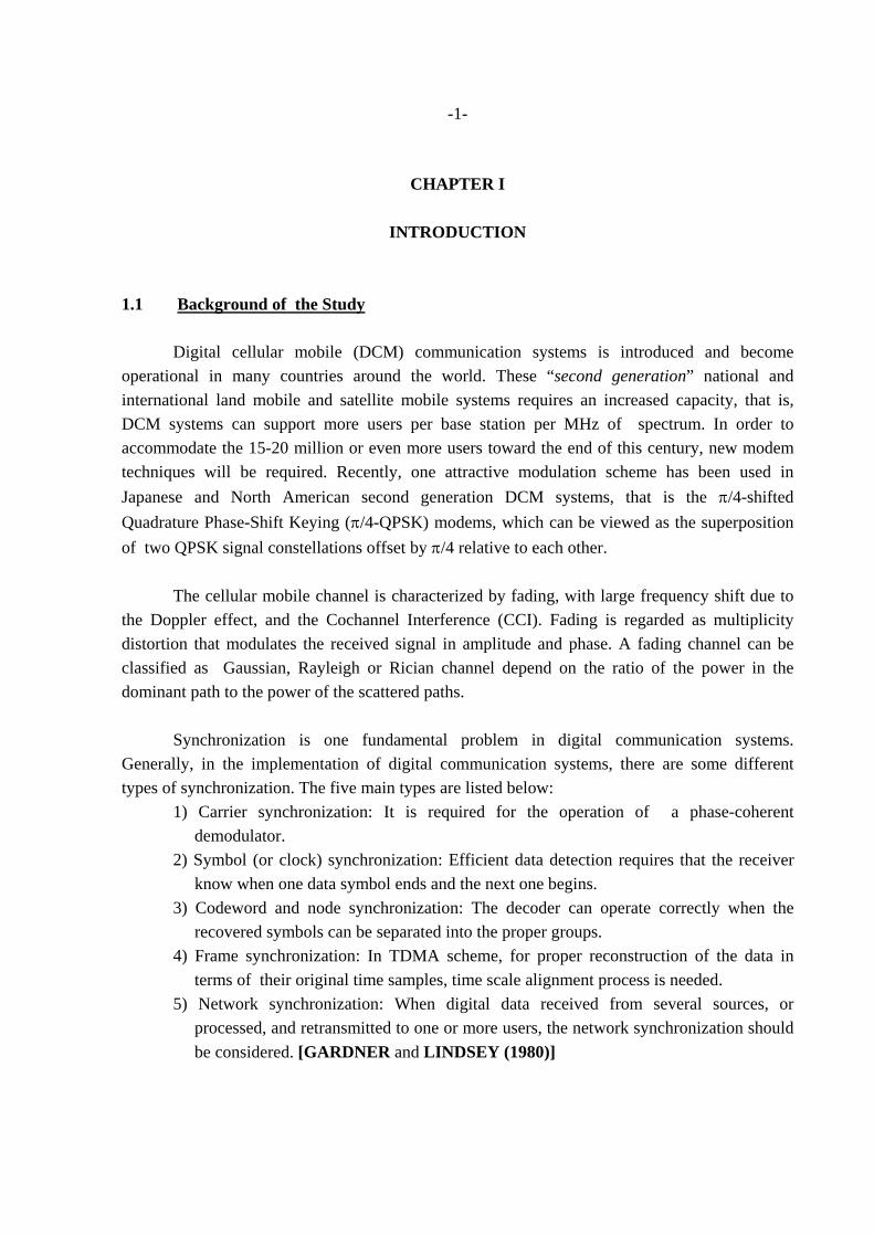
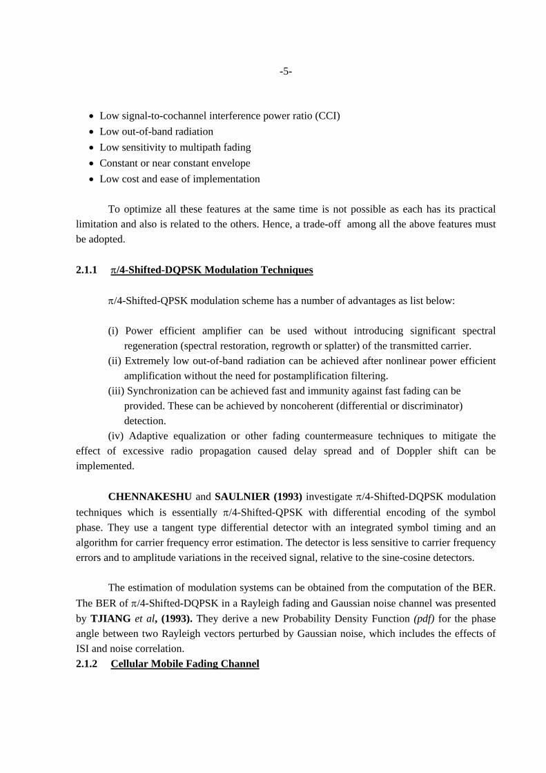
In cellular radio over fading channels, the received signal is not only corrupted by the AWGN noise, but also randomly perturbed in both amplitude and phase. To analyze the performance of mobile communications systems, a statistical model and computer simulation to regenerate the channel profiles at different receiving locations are required. STEELE (1992) describes some typical channel models. The simplest practical mathematical model is Gaussian channel, which models only the noise that is generated at the receiver, and provides an upper bound for performance of mobile communications systems. When all multipath components of the received signal manifest themselves as a group with negligible delay spread between them, the fading channel has Rayleigh pdf, and can be generated by its real and imaginary parts from two independent Gaussian noise sources.

White GaussianNoise Source

White GaussianNoise Source

DopplerFIlter

DopplerFilter

⊕ ⊗

⊗ ⊕

Additive WhiteGaussian Noise

TransmittedSignal

ReceivedSignal

j

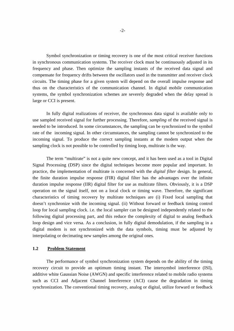
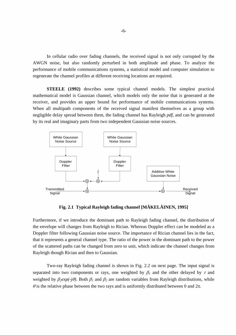
Fig. 2.1 Typical Rayleigh fading channel [MÄKELÄINEN, 1995] Furthermore, if we introduce the dominant path to Rayleigh fading channel, the distribution of the envelope will changes from Rayleigh to Rician. Whereas Doppler effect can be modeled as a Doppler filter following Gaussian noise source. The importance of Rician channel lies in the fact, that it represents a general channel type. The ratio of the power in the dominant path to the power of the scattered paths can be changed from zero to unit, which indicate the channel changes from Rayleigh though Rician and then to Gaussian. Two-ray Rayleigh fading channel is shown in Fig. 2.2 on next page. The input signal is separated into two components or rays, one weighted by β1 and the other delayed by τ and weighted by β2exp(-jθ). Both β1 and β2 are random variables from Rayleigh distributions, while θ is the relative phase between the two rays and is uniformly distributed between 0 and 2π.

-7-

MÄKELÄINEN (1995) indicates that in wideband channels, the bandwidth of the transmitted signal is greater than the coherence bandwidth of the channel, or correspondingly the

⊗

⊗

⊕

D

Input Output

β1

β2exp(-jθ)

Fig. 2.2 Two-rays Rayleigh fading channel model [STEELE, 1992]

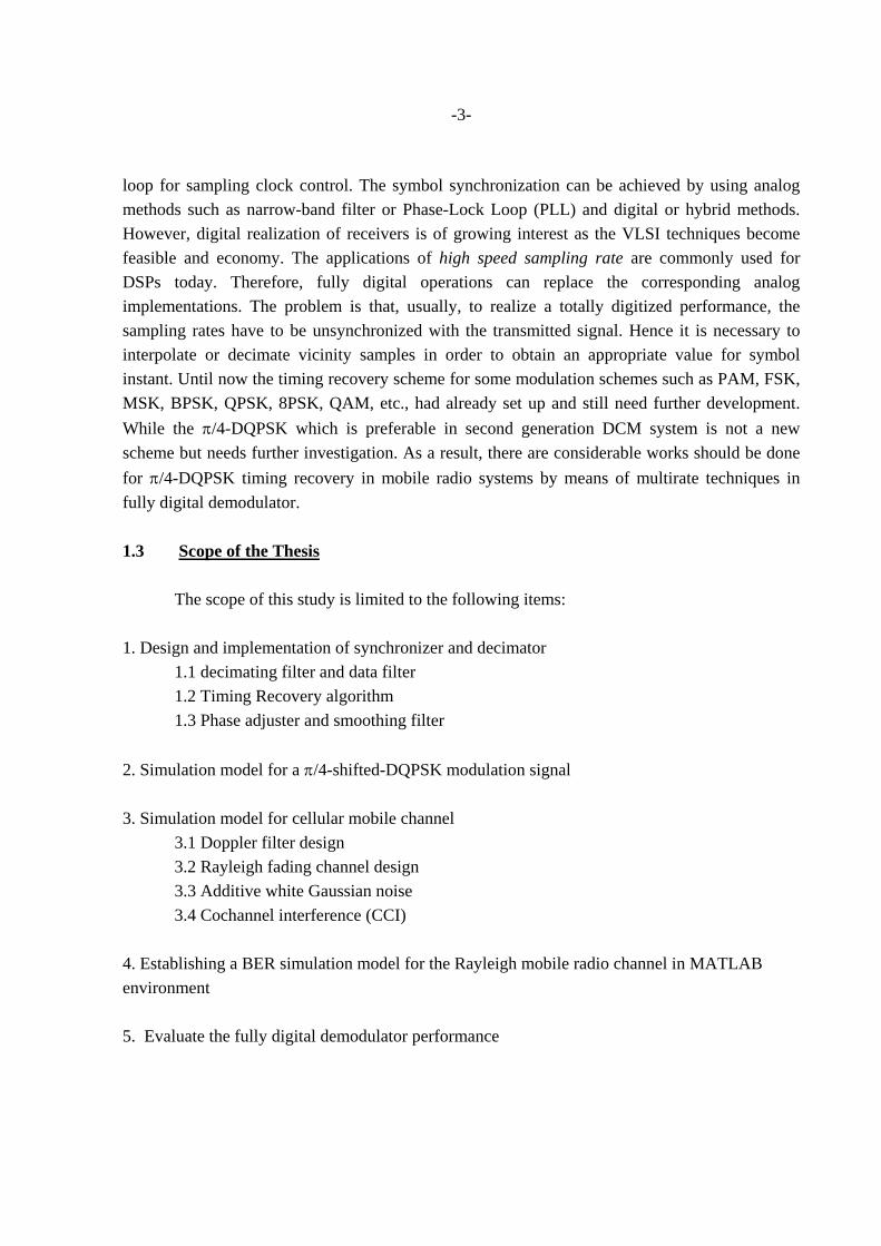
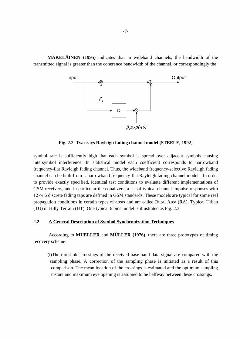
symbol rate is sufficiently high that each symbol is spread over adjacent symbols causing intersymbol interference. In statistical model each coefficient corresponds to narrowband frequency-flat Rayleigh fading channel. Thus, the wideband frequency-selective Rayleigh fading channel can be built from L narrowband frequency-flat Rayleigh fading channel models. In order to provide exactly specified, identical test conditions to evaluate different implementations of GSM receivers, and in particular the equalizers, a set of typical channel impulse responses with 12 or 6 discrete fading taps are defined in GSM standards. These models are typical for some real propagation conditions in certain types of areas and are called Rural Area (RA), Typical Urban (TU) or Hilly Terrain (HT). One typical 6 bins model is illustrated as Fig. 2.3 2.2 A General Description of Symbol Synchronization Techniques According to MUELLER and MÜLLER (1976), there are three prototypes of timing recovery scheme: (i)The threshold crossings of the received base-band data signal are compared with the sampling phase. A correction of the sampling phase is initiated as a result of this comparison. The mean location of the crossings is estimated and the optimum sampling instant and maximum eye opening is assumed to be halfway between these crossings.

-8-

White GaussianNoise Source

White GaussianNoise Source

DopplerFilter

DopplerFilter

⊗⊕

⊗

j

TransmittedSignal D

White GaussianNoise Source

White GaussianNoise Source

DopplerFilter

DopplerFilter

⊗⊕

⊗

j

D

⊕

White GaussianNoise Source

White GaussianNoise Source

DopplerFilter

DopplerFilter

⊗⊕

⊗

j

⊕

Additive WhiteGaussian Noise

⊕ ReceivedSignal

Fig. 2.3 Wideband frequency-selective Rayleigh fading channel model

[MÄKELÄINEN, 1995] (ii) The signal derivative can be used at the sampling instants. This derivative, or at least its sign, is usually correlated with the estimated data to produce the updating information required for the timing control loop. The resulting sampling phase is such that the mean square error between the signal and the appropriate reference levels is minimized, or, with slight changes. Such that sampling will occur at the peak of the impulse response. (iii) There is another method considered in frequency domain. A spectral line at the clock frequency (or at a multiple of this frequency) is filtered out with a narrow-band loop. An advantage of these systems is their ability to work with either the baseband or the passband signal. Practically, symbol synchronization is suitable for use in totally digital receivers that can be implemented with VLSI techniques. The method can be divided into two groups: the first in which sampling is performed at the symbol rate, and the second in which sampling is at a higher rate. Timing recovery in symbol-rate sampling is a well know synchronization method, the sampler operates coincided with transmitted symbol rate. Advantages of symbol-rate sampling are the simplicity in circuit design and economy. However, the signal samples which are used to derive symbol synchronization must also be utilized for other receiver functions such as equalization and threshold detection. MUELLER and MÜLLER demonstrated how useful timing functions could be derived from symbol-rate samples of pulses with raised-cosine spectra,

-9-

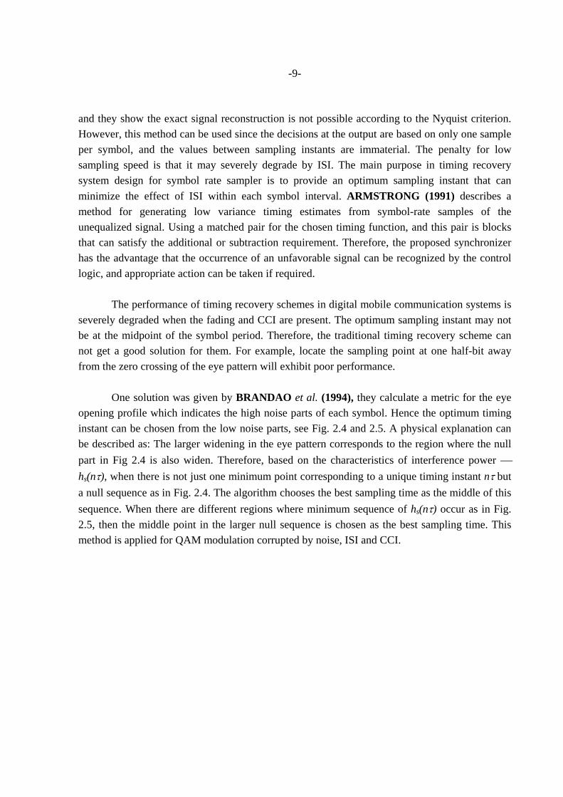
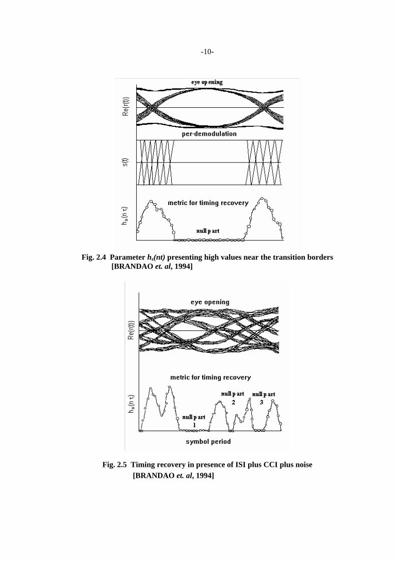
and they show the exact signal reconstruction is not possible according to the Nyquist criterion. However, this method can be used since the decisions at the output are based on only one sample per symbol, and the values between sampling instants are immaterial. The penalty for low sampling speed is that it may severely degrade by ISI. The main purpose in timing recovery system design for symbol rate sampler is to provide an optimum sampling instant that can minimize the effect of ISI within each symbol interval. ARMSTRONG (1991) describes a method for generating low variance timing estimates from symbol-rate samples of the unequalized signal. Using a matched pair for the chosen timing function, and this pair is blocks that can satisfy the additional or subtraction requirement. Therefore, the proposed synchronizer has the advantage that the occurrence of an unfavorable signal can be recognized by the control logic, and appropriate action can be taken if required. The performance of timing recovery schemes in digital mobile communication systems is severely degraded when the fading and CCI are present. The optimum sampling instant may not be at the midpoint of the symbol period. Therefore, the traditional timing recovery scheme can not get a good solution for them. For example, locate the sampling point at one half-bit away from the zero crossing of the eye pattern will exhibit poor performance. One solution was given by BRANDAO et al. (1994), they calculate a metric for the eye opening profile which indicates the high noise parts of each symbol. Hence the optimum timing instant can be chosen from the low noise parts, see Fig. 2.4 and 2.5. A physical explanation can be described as: The larger widening in the eye pattern corresponds to the region where the null part in Fig 2.4 is also widen. Therefore, based on the characteristics of interference power ⎯ hs(nτ), when there is not just one minimum point corresponding to a unique timing instant nτ but a null sequence as in Fig. 2.4. The algorithm chooses the best sampling time as the middle of this sequence. When there are different regions where minimum sequence of hs(nτ) occur as in Fig. 2.5, then the middle point in the larger null sequence is chosen as the best sampling time. This method is applied for QAM modulation corrupted by noise, ISI and CCI.

-10-

Fig. 2.4 Parameter hs(nt) presenting high values near the transition borders

[BRANDAO et. al, 1994]

Fig. 2.5 Timing recovery in presence of ISI plus CCI plus noise [BRANDAO et. al, 1994]

-11-

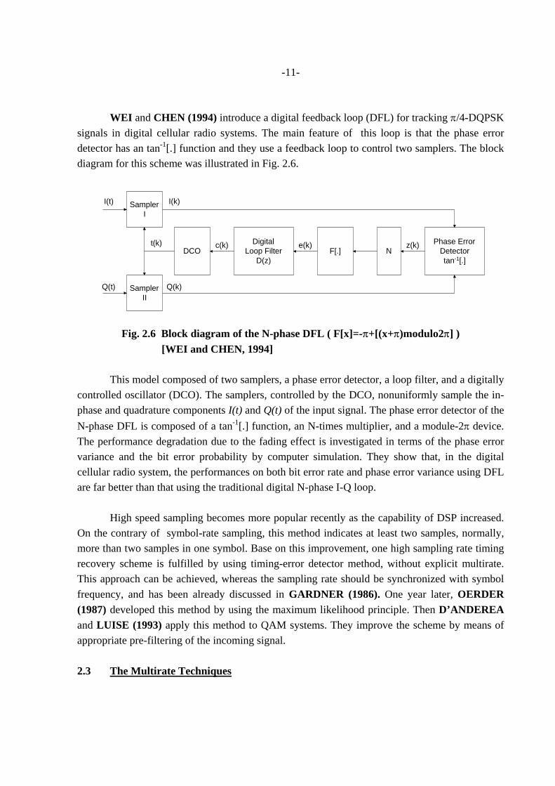
WEI and CHEN (1994) introduce a digital feedback loop (DFL) for tracking π/4-DQPSK signals in digital cellular radio systems. The main feature of this loop is that the phase error detector has an tan-1[.] function and they use a feedback loop to control two samplers. The block diagram for this scheme was illustrated in Fig. 2.6.

SamplerI

SamplerII

DCODigital

Loop FilterD(z)

F[.]Phase Error

Detectortan-1[.]

N

I(t)

Q(t)

t(k)

I(k)

Q(k)

c(k) e(k) z(k)

Fig. 2.6 Block diagram of the N-phase DFL ( F[x]=-π+[(x+π)modulo2π] )

[WEI and CHEN, 1994] This model composed of two samplers, a phase error detector, a loop filter, and a digitally controlled oscillator (DCO). The samplers, controlled by the DCO, nonuniformly sample the in-phase and quadrature components I(t) and Q(t) of the input signal. The phase error detector of the N-phase DFL is composed of a tan-1[.] function, an N-times multiplier, and a module-2π device. The performance degradation due to the fading effect is investigated in terms of the phase error variance and the bit error probability by computer simulation. They show that, in the digital cellular radio system, the performances on both bit error rate and phase error variance using DFL are far better than that using the traditional digital N-phase I-Q loop. High speed sampling becomes more popular recently as the capability of DSP increased. On the contrary of symbol-rate sampling, this method indicates at least two samples, normally, more than two samples in one symbol. Base on this improvement, one high sampling rate timing recovery scheme is fulfilled by using timing-error detector method, without explicit multirate. This approach can be achieved, whereas the sampling rate should be synchronized with symbol frequency, and has been already discussed in GARDNER (1986). One year later, OERDER (1987) developed this method by using the maximum likelihood principle. Then D’ANDEREA and LUISE (1993) apply this method to QAM systems. They improve the scheme by means of appropriate pre-filtering of the incoming signal. 2.3 The Multirate Techniques

-12-

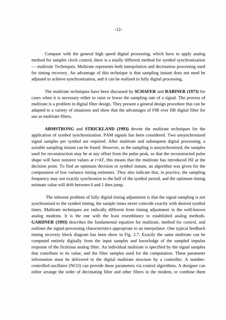
Compare with the general high speed digital processing, which have to apply analog method for sampler clock control, there is a totally different method for symbol synchronization ⎯ multirate Techniques. Multirate represents both interpolation and decimation processing used for timing recovery. An advantage of this technique is that sampling instant does not need be adjusted to achieve synchronization, and it can be realized in fully digital processing. The multirate techniques have been discussed by SCHAFER and RABINER (1973) for cases when it is necessary either to raise or lower the sampling rate of a signal. The process of multirate is a problem in digital filter design. They present a general design procedure that can be adapted to a variety of situations and show that the advantages of FIR over IIR digital filter for use as multirate filters. ARMSTRONG and STRICKLAND (1993) devote the multirate techniques for the application of symbol synchronization. PAM signals has been considered. Two unsynchronized signal samples per symbol are required. After multirate and subsequent digital processing, a suitable sampling instant can be found. However, as the sampling is unsynchronized, the samples used for reconstruction may be at any offset from the pulse peak, so that the reconstructed pulse shape will have nonzero values at t=kT, this means that the multirate has introduced ISI at the decision point. To find an optimum decision or symbol instant, an algorithm was given for the computation of low variance timing estimates. They also indicate that, in practice, the sampling frequency may not exactly synchronize to the half of the symbol period, and the optimum timing estimate value will drift between 0 and 1 then jump. The inherent problem of fully digital timing adjustment is that the signal sampling is not synchronized to the symbol timing, the sample times never coincide exactly with desired symbol times. Multirate techniques are radically different from timing adjustment in the well-known analog modems. It is the one with the least resemblance to established analog methods. GARDNER (1993) describes the fundamental equation for multirate, method for control, and outlines the signal-processing characteristics appropriate to an interpolator. One typical feedback timing recovery block diagram has been show in Fig. 2.7. Exactly the same multirate can be computed entirely digitally from the input samples and knowledge of the sampled impulse response of the fictitious analog filter. An individual multirate is specified by the signal samples that contribute to its value, and the filter samples used for the computation. These parameter information must be delivered to the digital multirate structure by a controller. A number-controlled oscillator (NCO) can provide these parameters via control algorithms. A designer can either arrange the order of decimating filter and other filters in the modem, or combine them

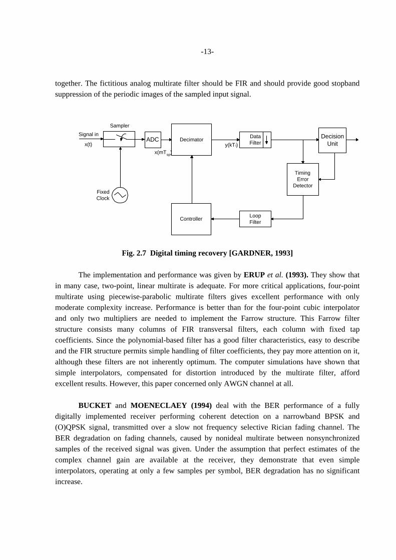
-13-

together. The fictitious analog multirate filter should be FIR and should provide good stopband suppression of the periodic images of the sampled input signal.

Decimator DataFilter

TimingError

Detector

LoopFilterController

SamplerSignal in

x(t)x(mTsp)

y(kTi)

FixedClock

ADC DecisionUnit

Fig. 2.7 Digital timing recovery [GARDNER, 1993] The implementation and performance was given by ERUP et al. (1993). They show that in many case, two-point, linear multirate is adequate. For more critical applications, four-point multirate using piecewise-parabolic multirate filters gives excellent performance with only moderate complexity increase. Performance is better than for the four-point cubic interpolator and only two multipliers are needed to implement the Farrow structure. This Farrow filter structure consists many columns of FIR transversal filters, each column with fixed tap coefficients. Since the polynomial-based filter has a good filter characteristics, easy to describe and the FIR structure permits simple handling of filter coefficients, they pay more attention on it, although these filters are not inherently optimum. The computer simulations have shown that simple interpolators, compensated for distortion introduced by the multirate filter, afford excellent results. However, this paper concerned only AWGN channel at all. BUCKET and MOENECLAEY (1994) deal with the BER performance of a fully digitally implemented receiver performing coherent detection on a narrowband BPSK and (O)QPSK signal, transmitted over a slow not frequency selective Rician fading channel. The BER degradation on fading channels, caused by nonideal multirate between nonsynchronized samples of the received signal was given. Under the assumption that perfect estimates of the complex channel gain are available at the receiver, they demonstrate that even simple interpolators, operating at only a few samples per symbol, BER degradation has no significant increase.

-14-

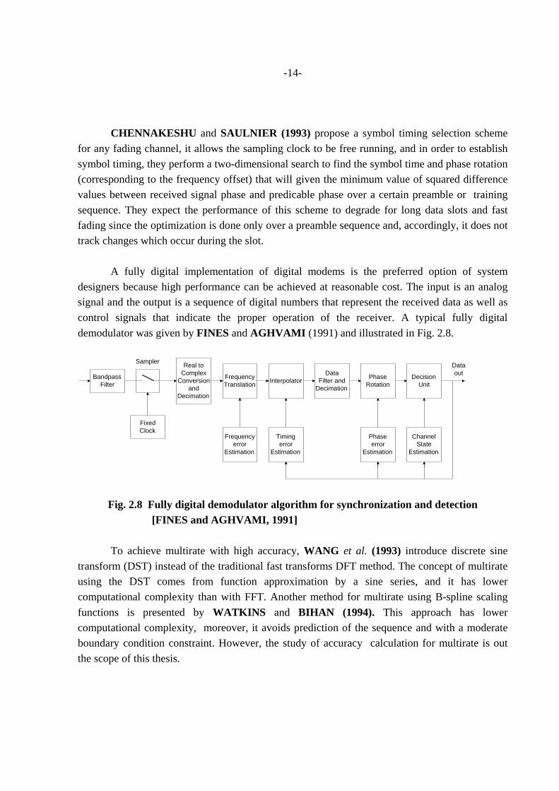
CHENNAKESHU and SAULNIER (1993) propose a symbol timing selection scheme for any fading channel, it allows the sampling clock to be free running, and in order to establish symbol timing, they perform a two-dimensional search to find the symbol time and phase rotation (corresponding to the frequency offset) that will given the minimum value of squared difference values between received signal phase and predicable phase over a certain preamble or training sequence. They expect the performance of this scheme to degrade for long data slots and fast fading since the optimization is done only over a preamble sequence and, accordingly, it does not track changes which occur during the slot. A fully digital implementation of digital modems is the preferred option of system designers because high performance can be achieved at reasonable cost. The input is an analog signal and the output is a sequence of digital numbers that represent the received data as well as control signals that indicate the proper operation of the receiver. A typical fully digital demodulator was given by FINES and AGHVAMI (1991) and illustrated in Fig. 2.8.

BandpassFilter

FixedClock

Real toComplex

Conversionand

Decimation

FrequencyTranslation Interpolator

DataFilter and

Decimation

PhaseRotation

DecisionUnit

Frequencyerror

Estimation

Timingerror

Estimation

Phaseerror

Estimation

ChannelState

Estimation

Sampler Dataout

Fig. 2.8 Fully digital demodulator algorithm for synchronization and detection [FINES and AGHVAMI, 1991] To achieve multirate with high accuracy, WANG et al. (1993) introduce discrete sine transform (DST) instead of the traditional fast transforms DFT method. The concept of multirate using the DST comes from function approximation by a sine series, and it has lower computational complexity than with FFT. Another method for multirate using B-spline scaling functions is presented by WATKINS and BIHAN (1994). This approach has lower computational complexity, moreover, it avoids prediction of the sequence and with a moderate boundary condition constraint. However, the study of accuracy calculation for multirate is out the scope of this thesis.

-16-

CHAPTER III

METHODOLOGY

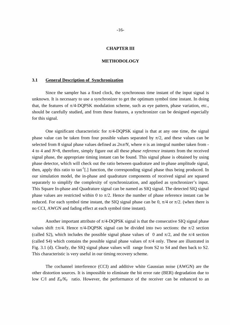
3.1 General Description of Synchronization Since the sampler has a fixed clock, the synchronous time instant of the input signal is unknown. It is necessary to use a synchronizer to get the optimum symbol time instant. In doing that, the features of π/4-DQPSK modulation scheme, such as eye pattern, phase variation, etc., should be carefully studied, and from these features, a synchronizer can be designed especially for this signal. One significant characteristic for π/4-DQPSK signal is that at any one time, the signal phase value can be taken from four possible values separated by π/2, and these values can be selected from 8 signal phase values defined as 2nπ/N, where n is an integral number taken from -4 to 4 and N=8, therefore, simply figure out all these phase reference instants from the received signal phase, the appropriate timing instant can be found. This signal phase is obtained by using phase detector, which will check out the ratio between quadrature and in-phase amplitude signal, then, apply this ratio to tan-1[.] function, the corresponding signal phase thus being produced. In our simulation model, the in-phase and quadrature components of received signal are squared separately to simplify the complexity of synchronization, and applied as synchronizer’s input. This Square In-phase and Quadrature signal can be named as SIQ signal. The detected SIQ signal phase values are restricted within 0 to π/2. Hence the number of phase reference instant can be reduced. For each symbol time instant, the SIQ signal phase can be 0, π/4 or π/2. (when there is no CCI, AWGN and fading effect at each symbol time instant). Another important attribute of π/4-DQPSK signal is that the consecutive SIQ signal phase values shift ±π/4. Hence π/4-DQPSK signal can be divided into two sections: the π/2 section (called S2), which includes the possible signal phase values of 0 and π/2, and the π/4 section (called S4) which contains the possible signal phase values of π/4 only. These are illustrated in Fig. 3.1 (d). Clearly, the SIQ signal phase values will range from S2 to S4 and then back to S2. This characteristic is very useful in our timing recovery scheme. The cochannel interference (CCI) and additive white Gaussian noise (AWGN) are the other distortion sources. It is impossible to eliminate the bit error rate (BER) degradation due to low C/I and Eb/N0 ratio. However, the performance of the receiver can be enhanced to an

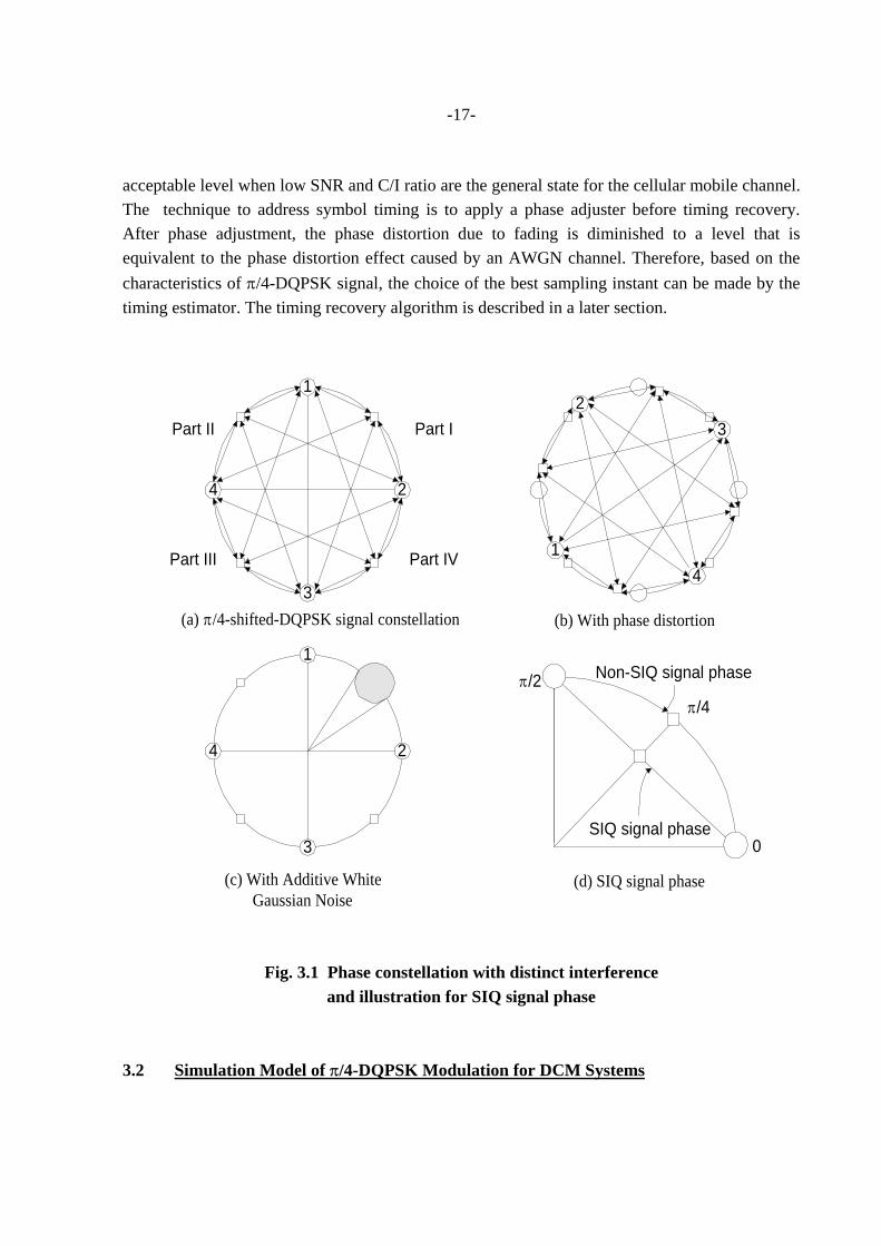
-17-

acceptable level when low SNR and C/I ratio are the general state for the cellular mobile channel. The technique to address symbol timing is to apply a phase adjuster before timing recovery. After phase adjustment, the phase distortion due to fading is diminished to a level that is equivalent to the phase distortion effect caused by an AWGN channel. Therefore, based on the characteristics of π/4-DQPSK signal, the choice of the best sampling instant can be made by the timing estimator. The timing recovery algorithm is described in a later section.

(b) With phase distortion

(c) With Additive WhiteGaussian Noise

(a) π/4-shifted-DQPSK signal constellation

1

2

3

4

2

14

3

1

2

3

4

π/2π/4

0

Part IPart II

Part III Part IV

(d) SIQ signal phase

Non-SIQ signal phase

SIQ signal phase

Fig. 3.1 Phase constellation with distinct interference and illustration for SIQ signal phase

3.2 Simulation Model of π/4-DQPSK Modulation for DCM Systems

-18-

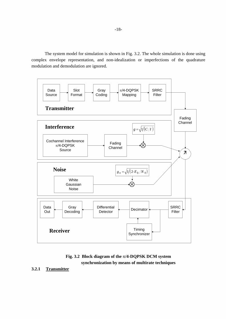
The system model for simulation is shown in Fig. 3.2. The whole simulation is done using complex envelope representation, and non-idealization or imperfections of the quadrature modulation and demodulation are ignored.

DataSource

GrayCoding

π/4-DQPSKMapping

SRRCFilter

FadingChannel

TimingSynchronizer

DecimatorDifferentialDetector

SRRCFilter

GrayDecoding

DataOut

WhiteGaussian

Noise

Cochannel Interferenceπ/4-DQPSK

Source

FadingChannel ⊗

⊗

Receiver

Interference

Transmitter

SlotFormat

Noise

( )g C I= 1

( )g E Nn b= ⋅1 2 0

Fig. 3.2 Block diagram of the π/4-DQPSK DCM system synchronization by means of multirate techniques

3.2.1 Transmitter

-19-

Assume input signal is a pseudo-random binary (PRB) data sequence which represent the desired transmitted data. The binary data signal is added with the training sequence and the other control signals in slot format unit. Then the signal to be transmitted can be represented by phase different ∆θ based on Gray coding (see Appendix A). The output signal of the modulator will be transmitted through a cellular mobile channel. The transmitted phase of π/4-DQPSK signal is given by θ θk k k= +−1 ∆θ , (3.1) where k represents symbol index. The transmitted signal for the mth sample can thus be written

as

( ) ( )r t e tk mj t

m kt

k m

m

( )= ⋅ −⋅

=−∞

∞

∑ θ δ ξ , (3.2)

where ξk is the kth synchronized time instant, and δ(t) is the Dirac delta function. In order to reduce the transmission bandwidth and for better receiver processing. Two Square Root Raised Cosine filter (SRRC) are used, one at the transmitter and the other at the receiver. The first time filtering output is ( ) ( ) ( )x t h t r tk m k m= ∗ , (3.3) where h(t) is the impulse response of SRRC filter, and the asterisk indicates convolution. In this thesis, assume that the carrier is perfectly synchronized. Therefore only complex envelope is considered. The channel model used in simulation is selected based on the propagation environment. Generally, for a fading channel with interference and noise, the kth received signal is described as:

( ) ( ) ( )[ ] ( ) ( )y t x t e c t n tk m k mj t

k m k mk m= ⋅ + +⋅ µ , (3.4)

where µ(t) is the channel-induced phase distortion, c(t) is the composite interfering signal (e.g., CCI and ACI) and n(t) is the AWGN component with zero mean and variance σn 2.

-20-

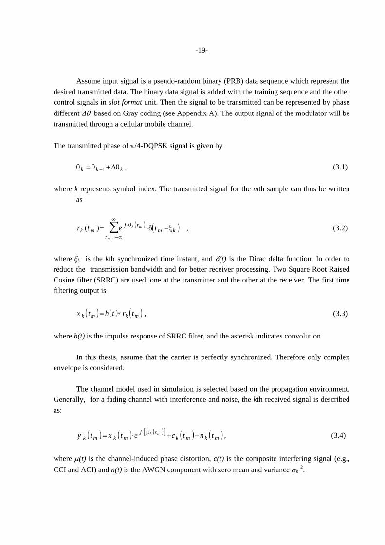
The SRRC filter at the receiver, which is the so-called data filter, is used to eliminate ISI introduced by the same filter at the transmitter. The out-of-band noise from the channel can be excluded as well. In this system, SRRC filter also be used as decimating filter, and it accomplishes a signal reconstruction task for decimation. The output of the filter is ( ) ( ) ( )z t h t y tk m k m= ∗ . (3.5) 3.2.2 Model of the Receiver In a cellular mobile system, the effect of fading and CCI must be considered. Therefore, more attention should be paid to the timing recovery. One approach for receiver design is shown in Fig. 3.3. The complex signal input will be divided into in-phase and quadrature components first, and then employed for the timing recovery unit and decimator simultaneously. The timing recovery unit is specifically designed for cellular mobile system. The given appropriate timing instant from the timing unit is used first by controller and then by the decimator. The high sampling rate is reduced to symbol rate by decimator. The spectrum of decimating filter is a square-root-raised-cosine with a proper roll-off equal to 0.35. The smoothing filter diminishes noise, and defines the loop bandwidth. Finally, differential detector (DD) is used to get the transmitted data sequence.

TimingRecovery

Unit

Decimator DecisionUnit

SmoothingFilter

Sampling rate1/Tsp

1/T

Symbol rate1/T

Inphase & quadrature

Legend

Symbol rate1/T

Symbol rate1/T

Fig. 3.3 Multirate receiver model [Adapted from GARDNER, 1993] 3.2.3 Simulation Model of Synchronizer

-21-

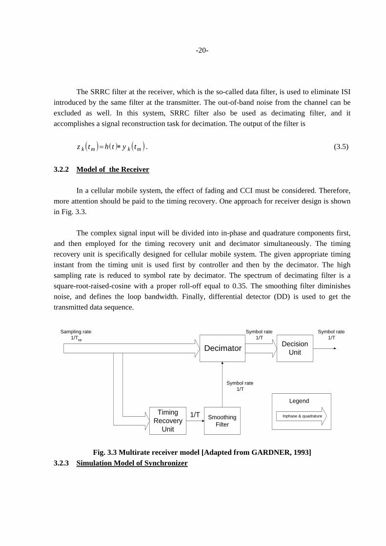
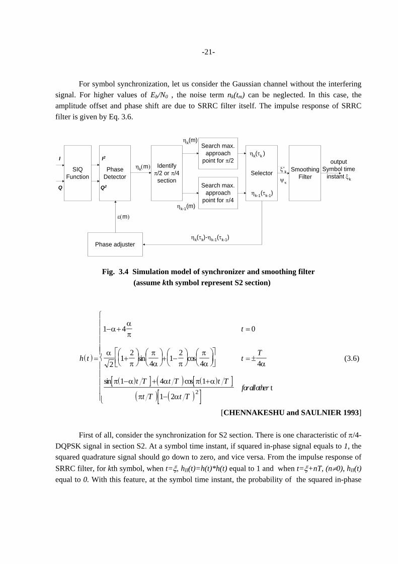
For symbol synchronization, let us consider the Gaussian channel without the interfering signal. For higher values of Eb/N0 , the noise term nk(tm) can be neglected. In this case, the amplitude offset and phase shift are due to SRRC filter itself. The impulse response of SRRC filter is given by Eq. 3.6.

PhaseDetector

Search max.approach

point for π/2

Search max.approach

point for π/4

Identifyπ/2 or π/4section

Selector SmoothingFilter

I2

Q2

outputSymbol time

instant ξk

ηk(m)

ηk(m)

ηk-1(m)

ηk(τk )

ηk-1(τk-1)

SIQFunction

I

Q

Phase adjusterηk(τk)-ηk-1(τk-1)

ε(m)

ξ'kψκ

Fig. 3.4 Simulation model of synchronizer and smoothing filter

(assume kth symbol represent S2 section)

( )

( )[ ] ( ) ( )[ ]( ) ( )[ ]

h t

t

tT

t T t T t T

t T t Tforallother

=

− + =

+⎛⎝⎜

⎞⎠⎟

⎛⎝⎜

⎞⎠⎟+ −

⎛⎝⎜

⎞⎠⎟

⎛⎝⎜

⎞⎠⎟

⎡⎣⎢

⎤⎦⎥

= ±

− + +

−

⎧

⎨

⎪⎪⎪⎪⎪

⎩

⎪⎪⎪⎪⎪

1 4 0

21

24

12

4 4

1 4 1

1 22

ααπ

απ

πα π

πα α

π α α π α

π α

sin cos

sin cos t

(3.6)

[CHENNAKESHU and SAULNIER 1993] First of all, consider the synchronization for S2 section. There is one characteristic of π/4-DQPSK signal in section S2. At a symbol time instant, if squared in-phase signal equals to 1, the squared quadrature signal should go down to zero, and vice versa. From the impulse response of SRRC filter, for kth symbol, when t=ξ, hII(t)=h(t)*h(t) equal to 1 and when t=ξ+nT, (n≠0), hII(t) equal to 0. With this feature, at the symbol time instant, the probability of the squared in-phase

-22-

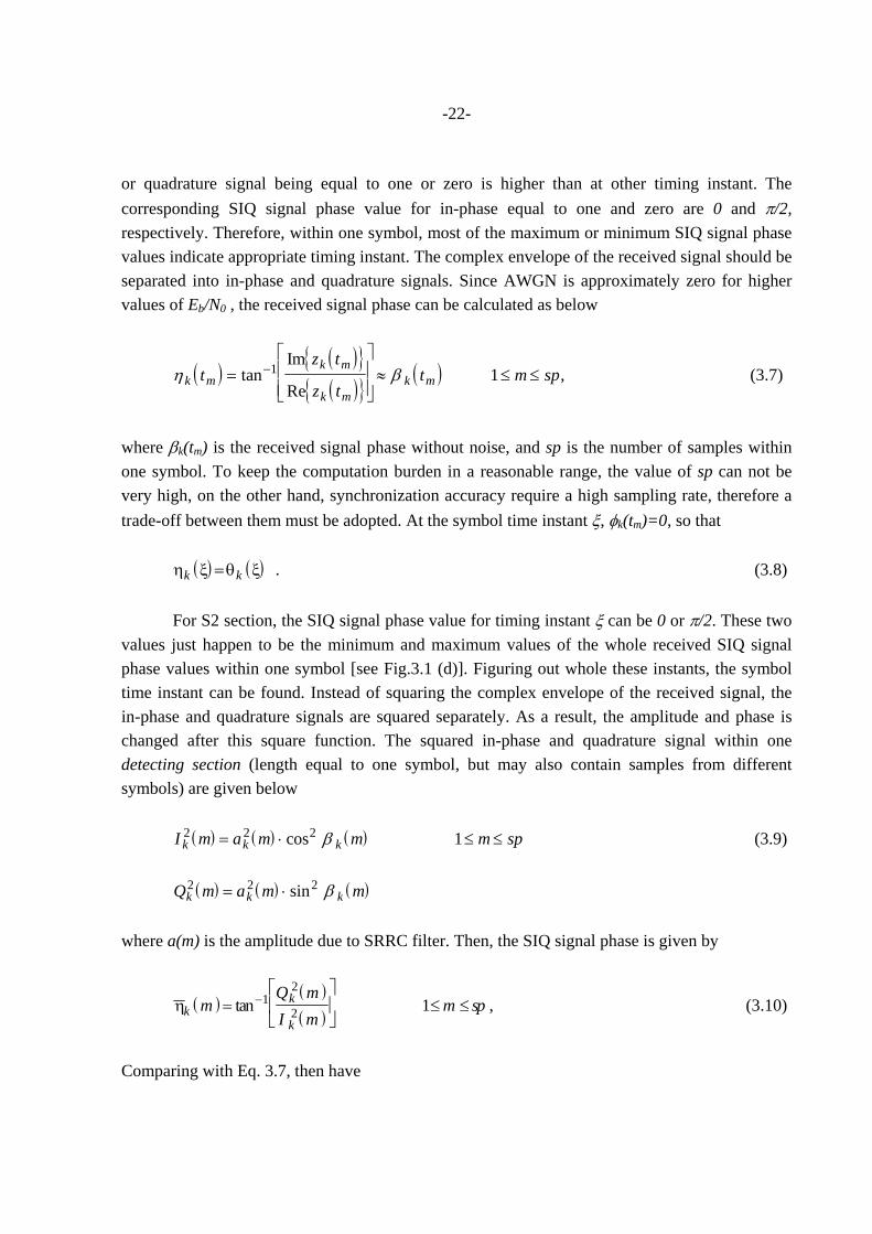
or quadrature signal being equal to one or zero is higher than at other timing instant. The corresponding SIQ signal phase value for in-phase equal to one and zero are 0 and π/2, respectively. Therefore, within one symbol, most of the maximum or minimum SIQ signal phase values indicate appropriate timing instant. The complex envelope of the received signal should be separated into in-phase and quadrature signals. Since AWGN is approximately zero for higher values of Eb/N0 , the received signal phase can be calculated as below

( )( ){ }( ){ }

( )η βk mk m

k mk mt

z t

z tt m sp=

⎡

⎣⎢⎢

⎤

⎦⎥⎥

≈ ≤ ≤−tanIm

Re1 1 , (3.7)

where βk(tm) is the received signal phase without noise, and sp is the number of samples within one symbol. To keep the computation burden in a reasonable range, the value of sp can not be very high, on the other hand, synchronization accuracy require a high sampling rate, therefore a trade-off between them must be adopted. At the symbol time instant ξ, φk(tm)=0, so that ( ) ( )η ξ θ ξk k= . (3.8) For S2 section, the SIQ signal phase value for timing instant ξ can be 0 or π/2. These two values just happen to be the minimum and maximum values of the whole received SIQ signal phase values within one symbol [see Fig.3.1 (d)]. Figuring out whole these instants, the symbol time instant can be found. Instead of squaring the complex envelope of the received signal, the in-phase and quadrature signals are squared separately. As a result, the amplitude and phase is changed after this square function. The squared in-phase and quadrature signal within one detecting section (length equal to one symbol, but may also contain samples from different symbols) are given below ( ) ( ) ( )I m a m m m spk k k

2 2 2 1= ⋅ ≤ ≤cos β (3.9) ( ) ( ) ( )Q m a m mk k k

2 2 2= ⋅ sin β where a(m) is the amplitude due to SRRC filter. Then, the SIQ signal phase is given by

( )( )( )

ηkk

km

Q mI m

m sp=⎡

⎣⎢

⎤

⎦⎥ ≤ ≤−tan 1

2

2 1 , (3.10)

Comparing with Eq. 3.7, then have

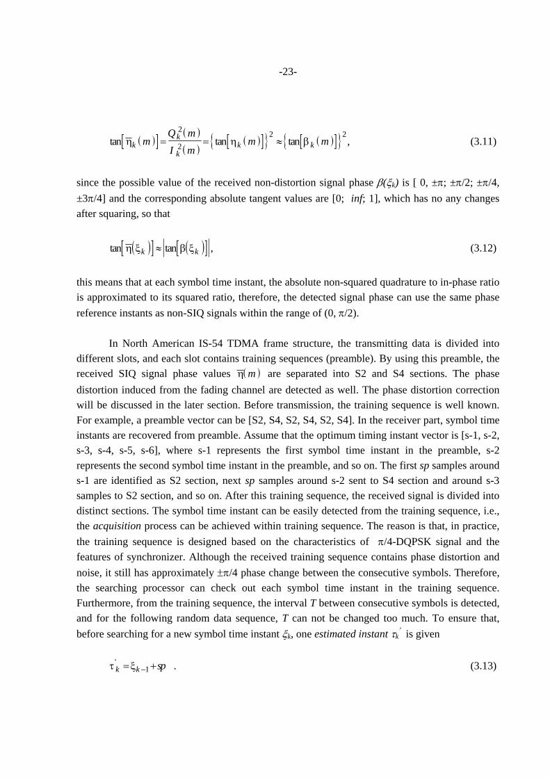
-23-

( )[ ] ( )( )

( )[ ]{ } ( )[ ]{ }tan tan tanη η βkk

kk km

Q mI m

m m= = ≈2

22 2

, (3.11)

since the possible value of the received non-distortion signal phase β(ξk) is [ 0, ±π; ±π/2; ±π/4, ±3π/4] and the corresponding absolute tangent values are [0; inf; 1], which has no any changes after squaring, so that

( )[ ] ( )[ ]tan tanη ξ β ξk k≈ , (3.12)

this means that at each symbol time instant, the absolute non-squared quadrature to in-phase ratio is approximated to its squared ratio, therefore, the detected signal phase can use the same phase reference instants as non-SIQ signals within the range of (0, π/2). In North American IS-54 TDMA frame structure, the transmitting data is divided into different slots, and each slot contains training sequences (preamble). By using this preamble, the received SIQ signal phase values ( )η m are separated into S2 and S4 sections. The phase distortion induced from the fading channel are detected as well. The phase distortion correction will be discussed in the later section. Before transmission, the training sequence is well known. For example, a preamble vector can be [S2, S4, S2, S4, S2, S4]. In the receiver part, symbol time instants are recovered from preamble. Assume that the optimum timing instant vector is [s-1, s-2, s-3, s-4, s-5, s-6], where s-1 represents the first symbol time instant in the preamble, s-2 represents the second symbol time instant in the preamble, and so on. The first sp samples around s-1 are identified as S2 section, next sp samples around s-2 sent to S4 section and around s-3 samples to S2 section, and so on. After this training sequence, the received signal is divided into distinct sections. The symbol time instant can be easily detected from the training sequence, i.e., the acquisition process can be achieved within training sequence. The reason is that, in practice, the training sequence is designed based on the characteristics of π/4-DQPSK signal and the features of synchronizer. Although the received training sequence contains phase distortion and noise, it still has approximately ±π/4 phase change between the consecutive symbols. Therefore, the searching processor can check out each symbol time instant in the training sequence. Furthermore, from the training sequence, the interval T between consecutive symbols is detected, and for the following random data sequence, T can not be changed too much. To ensure that, before searching for a new symbol time instant ξk, one estimated instant τk

′ is given τ ξk k sp' = +−1 . (3.13)

-24-

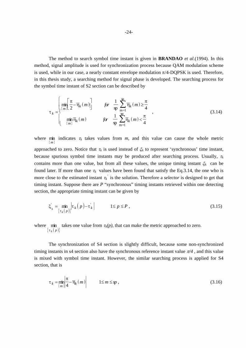
The method to search symbol time instant is given in BRANDAO et al.(1994). In this method, signal amplitude is used for synchronization process because QAM modulation scheme is used, while in our case, a nearly constant envelope modulation π/4-DQPSK is used. Therefore, in this thesis study, a searching method for signal phase is developed. The searching process for the symbol time instant of S2 section can be described by

{ }

( ) ( )

{ }( ) ( )

τ

πη η

π

η ηπk

mk k

mk k

m for m

m for m=

−⎡⎣⎢

⎤⎦⎥

≥

<

⎧

⎨⎪⎪

⎩⎪⎪

∑

∑

min

min

2 4

4

1sp

1sp

m=1

sp

m=1

sp , (3.14)

where

{ }minm

indicates τk takes values from m, and this value can cause the whole metric

approached to zero. Notice that τk is used instead of ξk to represent ‘synchronous’ time instant, because spurious symbol time instants may be produced after searching process. Usually, τk contains more than one value, but from all these values, the unique timing instant ξk can be found later. If more than one τk values have been found that satisfy the Eq.3.14, the one who is more close to the estimated instant τk

′ is the solution. Therefore a selector is designed to get that timing instant. Suppose there are P “synchronous” timing instants retrieved within one detecting section, the appropriate timing instant can be given by

( ){ }

( )ξ τ ττk

k pk kp p P' 'min= − ≤ ≤ 1 , (3.15)

where

( ){ }min

τ k p takes one value from τk(p), that can make the metric approached to zero.

The synchronization of S4 section is slightly difficult, because some non-synchronized timing instants in s4 section also have the synchronous reference instant value π/4 , and this value is mixed with symbol time instant. However, the similar searching process is applied for S4 section, that is

{ }

( )τπ

ηkm

k m m sp= − ≤ ≤min4

1 , (3.16)

-25-

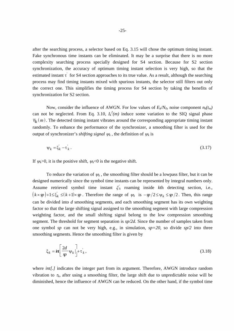
after the searching process, a selector based on Eq. 3.15 will chose the optimum timing instant. Fake synchronous time instants can be eliminated. It may be a surprise that there is no more complexity searching process specially designed for S4 section. Because for S2 section synchronization, the accuracy of optimum timing instant selection is very high, so that the estimated instant τ′ for S4 section approaches to its true value. As a result, although the searching process may find timing instants mixed with spurious instants, the selector still filters out only the correct one. This simplifies the timing process for S4 section by taking the benefits of synchronization for S2 section. Now, consider the influence of AWGN. For low values of Eb/N0, noise component nk(tm) can not be neglected. From Eq. 3.10, Ik

2(m) induce some variation to the SIQ signal phase ( )ηk m . The detected timing instant vibrates around the corresponding appropriate timing instant

randomly. To enhance the performance of the synchronizer, a smoothing filter is used for the output of synchronizer’s shifting signal ψk , the definition of ψk is ψ ξ τk k k= −' ' . (3.17) If ψk>0, it is the positive shift, ψk<0 is the negative shift. To reduce the variation of ψk , the smoothing filter should be a lowpass filter, but it can be designed numerically since the symbol time instants can be represented by integral numbers only. Assume retrieved symbol time instant ξ′

k roaming inside kth detecting section, i.e., ( ) ( )k sp k spk× + ≤ ≤ + ×1 1ξ' . Therefore the range of ψk is − ≤ ≤sp spk2 2ψ . Then, this range can be divided into d smoothing segments, and each smoothing segment has its own weighting factor so that the large shifting signal assigned to the smoothing segment with large compression weighting factor, and the small shifting signal belong to the low compression smoothing segment. The threshold for segment separation is sp/2d. Since the number of samples taken from one symbol sp can not be very high, e.g., in simulation, sp=20, so divide sp/2 into three smoothing segments. Hence the smoothing filter is given by

ξ ψ τk k kintd

sp=

⎡

⎣⎢⎤

⎦⎥+

2 ' , (3.18)

where int[.] indicates the integer part from its argument. Therefore, AWGN introduce random vibration to τk, after using a smoothing filter, the large shift due to unpredictable noise will be diminished, hence the influence of AWGN can be reduced. On the other hand, if the symbol time

-26-

instant is located far away from the estimated instant τk′, it will continuously move in the correct

direction, and finally, the detected time instant ξk can reach that destination symbol time instant. Obtaining the optimum timing instant of the signal received through the fading channel is the main purpose of the synchronizer. Comparing this with the AWGN channel, the fading channel induces amplitude aberration and phase distortion µ(t). Without these effects, the complexity of timing recovery decreased to the complexity of timing recovery with AWGN channel, whose synchronization has been discussed already. Naturally, the phase adjuster comes into mind. The phase adjuster can reduce the phase distortion caused by fading channel to an extent the phase distortion caused by AWGN channel. However, before discussing the phase correction scheme, the impairment of the phase distortion for π/4-DQPSK modulation signal has to be considered. Figure 3.1 (b) shows one possible location of π/4-DQPSK signal constellation shifted by µ(t). This phase distortion µ(t) is uniformly distributed from 0 to 2π. Therefore, it is impossible to estimate the value of µ(t) from the received signal without any training sequence. The training sequence can be used to initialize µ(t). Prior to transmitting, the signal phase value of this training sequence is well known. When the signal is received, phase can be changed to any value due to the fading channel effect. Practically, the estimated instant τk

′ is used for phase distortion estimation, that is

( ) ( )µ θ η τk Pk k mm mk

''= − = , (3.19)

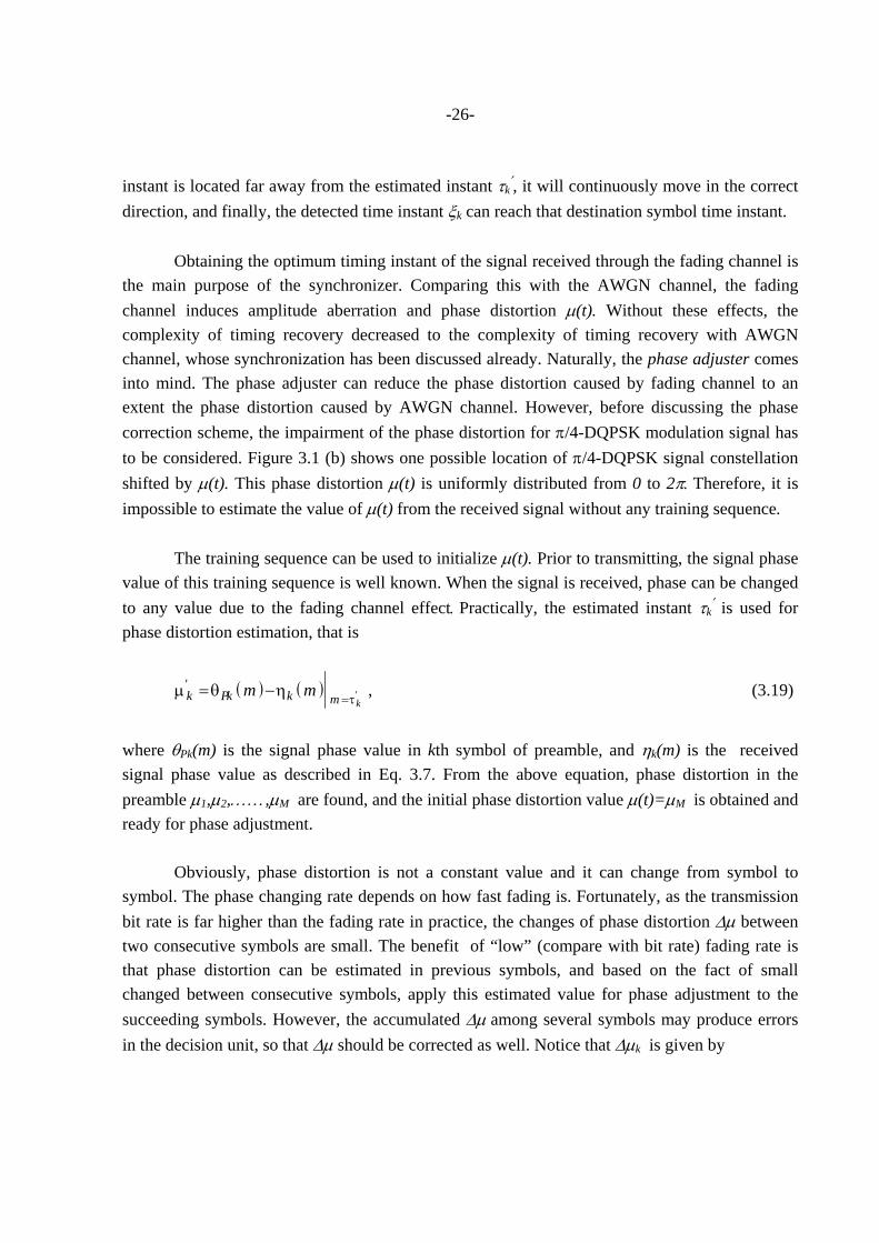
where θPk(m) is the signal phase value in kth symbol of preamble, and ηk(m) is the received signal phase value as described in Eq. 3.7. From the above equation, phase distortion in the preamble µ1,µ2,……,µM are found, and the initial phase distortion value µ(t)=µM is obtained and ready for phase adjustment. Obviously, phase distortion is not a constant value and it can change from symbol to symbol. The phase changing rate depends on how fast fading is. Fortunately, as the transmission bit rate is far higher than the fading rate in practice, the changes of phase distortion ∆µ between two consecutive symbols are small. The benefit of “low” (compare with bit rate) fading rate is that phase distortion can be estimated in previous symbols, and based on the fact of small changed between consecutive symbols, apply this estimated value for phase adjustment to the succeeding symbols. However, the accumulated ∆µ among several symbols may produce errors in the decision unit, so that ∆µ should be corrected as well. Notice that ∆µk is given by

-27-

( )( )∆µk

k k k k

k k k k=

− − >− + <

⎧⎨⎩

− −

− −

η η π η ηη η π η η

1 1

1 1

44

, (3.20)

hence the estimated correction factor (phase) is ( )ε µ µk k k k= − + = −−1

' '∆µ (3.21)

where µ′k represents the estimated phase distortion for the kth symbol. Before synchronous processing, the received signal phase should be corrected as

( ) ( ) ( )z t z t e m spk m k mj tk m' = ⋅ ≤ ≤⋅ε 1 , (3.22)

if the estimation is good enough, then ∆dk(tm)=µk(tm)-µk

′(tm)=0. Otherwise, the result of this subtraction also approaches to zero. After the adjustment, the phase distortion due to fading is reduced significantly, which satisfies synchronization conditions. Notice that in the simulation model, SIQ signal phase is used. From Fig. 3.1 (a), if the phases reside inside part I and part III, the SIQ signal phase can be shifted directly by ( )e j mk⋅ε ; if the phases are located inside part II and part IV, ( )e j mk⋅ε should be modified to its conjugation value, that is ( )e j mk− ⋅ε . 3.2.4 Decimation and Differential Detector The decimating filter is a SRRC filter as described in Eq. 3.6. The output of the decimating filter is a sampled signal sequence zk(tm). According to ξk , by simply choosing the corresponding samples from this signal sequence, decimation is accomplished. In the differential detector (DD), the input signal is multiplied by its one-symbol delay version.

-28-

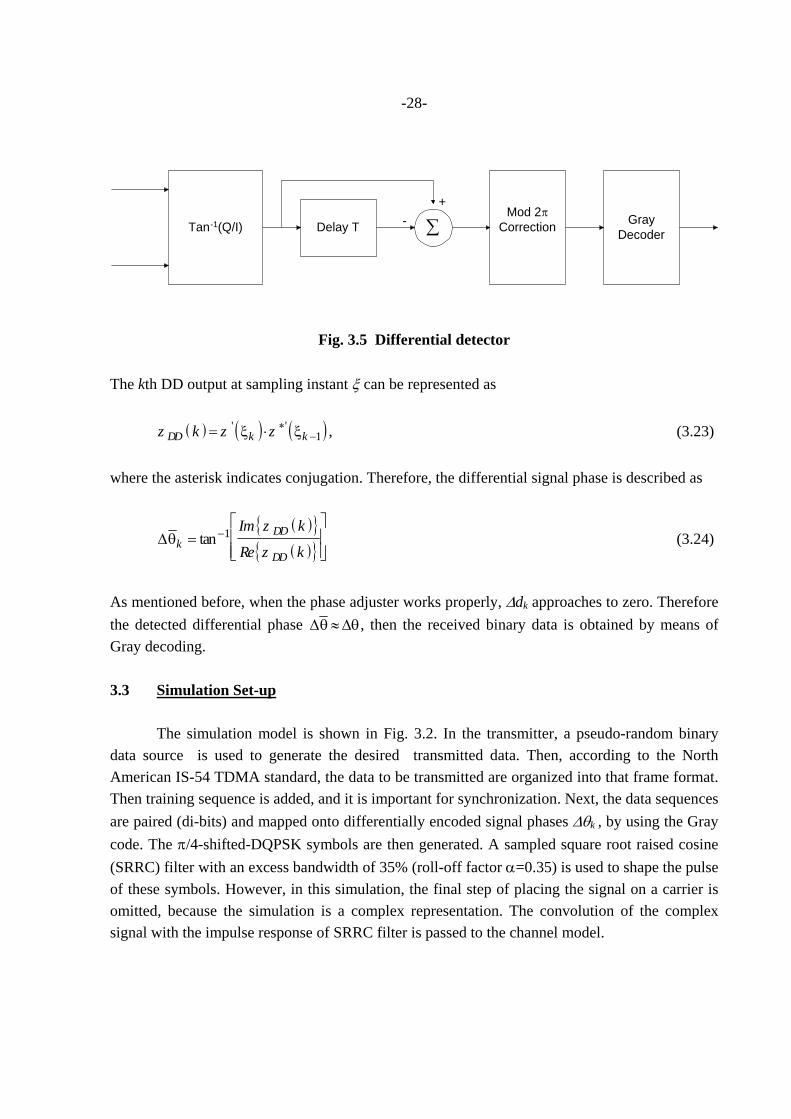
Tan-1(Q/I) Delay T ∑Mod 2π

Correction GrayDecoder

-+

Fig. 3.5 Differential detector The kth DD output at sampling instant ξ can be represented as ( ) ( ) ( )z k z zDD k k= ⋅ ∗

−' 'ξ ξ 1 , (3.23)

where the asterisk indicates conjugation. Therefore, the differential signal phase is described as

( ){ }( ){ }∆θk

DD

DD

Im z k

Re z k=

⎡

⎣⎢⎢

⎤

⎦⎥⎥

−tan 1 (3.24)

As mentioned before, when the phase adjuster works properly, ∆dk approaches to zero. Therefore the detected differential phase ∆ ∆θθ ≈ , then the received binary data is obtained by means of Gray decoding. 3.3 Simulation Set-up The simulation model is shown in Fig. 3.2. In the transmitter, a pseudo-random binary data source is used to generate the desired transmitted data. Then, according to the North American IS-54 TDMA standard, the data to be transmitted are organized into that frame format. Then training sequence is added, and it is important for synchronization. Next, the data sequences are paired (di-bits) and mapped onto differentially encoded signal phases ∆θk , by using the Gray code. The π/4-shifted-DQPSK symbols are then generated. A sampled square root raised cosine (SRRC) filter with an excess bandwidth of 35% (roll-off factor α=0.35) is used to shape the pulse of these symbols. However, in this simulation, the final step of placing the signal on a carrier is omitted, because the simulation is a complex representation. The convolution of the complex signal with the impulse response of SRRC filter is passed to the channel model.

-29-

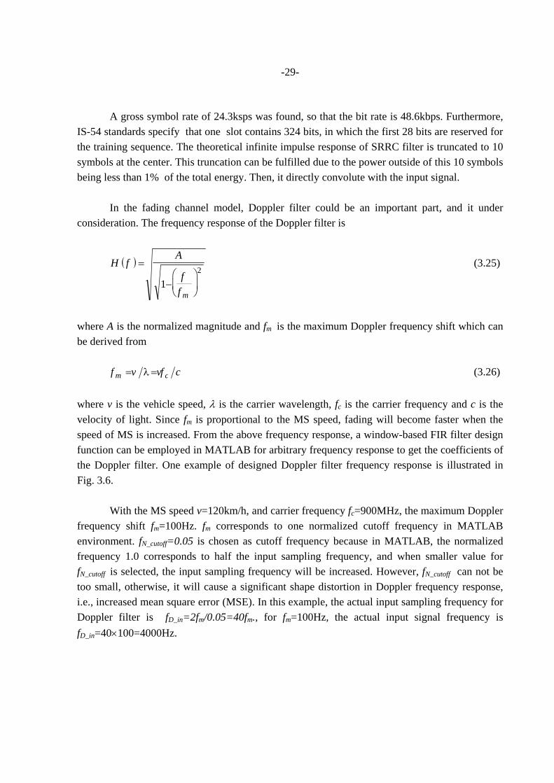
A gross symbol rate of 24.3ksps was found, so that the bit rate is 48.6kbps. Furthermore, IS-54 standards specify that one slot contains 324 bits, in which the first 28 bits are reserved for the training sequence. The theoretical infinite impulse response of SRRC filter is truncated to 10 symbols at the center. This truncation can be fulfilled due to the power outside of this 10 symbols being less than 1% of the total energy. Then, it directly convolute with the input signal. In the fading channel model, Doppler filter could be an important part, and it under consideration. The frequency response of the Doppler filter is

( )H fA

ff m

=

−⎛

⎝⎜

⎞

⎠⎟1

2 (3.25)

where A is the normalized magnitude and fm is the maximum Doppler frequency shift which can be derived from f v vf cm c= =λ (3.26) where v is the vehicle speed, λ is the carrier wavelength, fc is the carrier frequency and c is the velocity of light. Since fm is proportional to the MS speed, fading will become faster when the speed of MS is increased. From the above frequency response, a window-based FIR filter design function can be employed in MATLAB for arbitrary frequency response to get the coefficients of the Doppler filter. One example of designed Doppler filter frequency response is illustrated in Fig. 3.6. With the MS speed v=120km/h, and carrier frequency fc=900MHz, the maximum Doppler frequency shift fm=100Hz. fm corresponds to one normalized cutoff frequency in MATLAB environment. fN_cutoff=0.05 is chosen as cutoff frequency because in MATLAB, the normalized frequency 1.0 corresponds to half the input sampling frequency, and when smaller value for fN_cutoff is selected, the input sampling frequency will be increased. However, fN_cutoff can not be too small, otherwise, it will cause a significant shape distortion in Doppler frequency response, i.e., increased mean square error (MSE). In this example, the actual input sampling frequency for Doppler filter is fD_in=2fm/0.05=40fm., for fm=100Hz, the actual input signal frequency is fD_in=40×100=4000Hz.

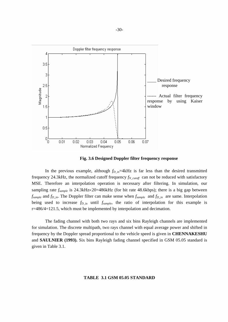
-30-

In the previous example, although fD_in=4kHz is far less than the desired transmitted frequency 24.3kHz, the normalized cutoff frequency fN_cutoff can not be reduced with satisfactory MSE. Therefore an interpolation operation is necessary after filtering. In simulation, our sampling rate fsample is 24.3kHz×20=486kHz (for bit rate 48.6kbps); there is a big gap between fsample and fD_in. The Doppler filter can make sense when fsample and fD_in are same. Interpolation being used to increase fD_in until fsample, the ratio of interpolation for this example is r=486/4=121.5, which must be implemented by interpolation and decimation. The fading channel with both two rays and six bins Rayleigh channels are implemented for simulation. The discrete multipath, two rays channel with equal average power and shifted in frequency by the Doppler spread proportional to the vehicle speed is given in CHENNAKESHU and SAULNIER (1993). Six bins Rayleigh fading channel specified in GSM 05.05 standard is given in Table 3.1.

TABLE 3.1 GSM 05.05 STANDARD

____ Desired frequency response ------ Actual filter frequency response by using Kaiser window

Fig. 3.6 Designed Doppler filter frequency response

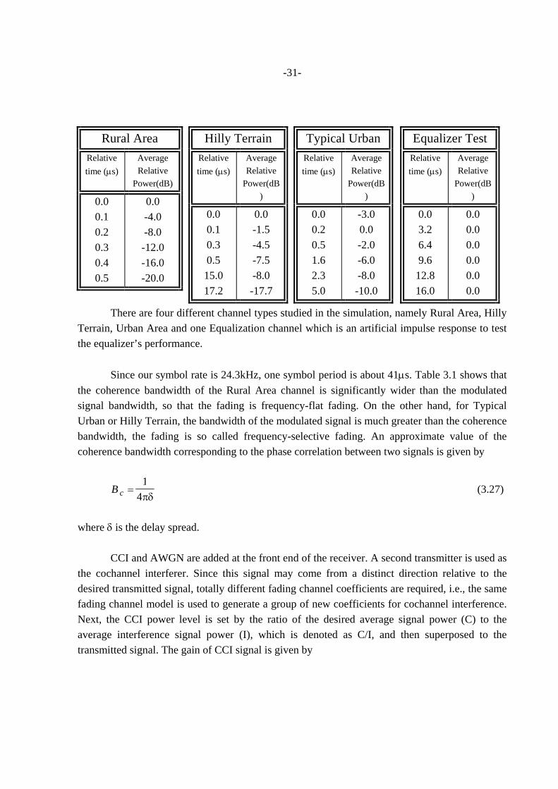
-31-

There are four different channel types studied in the simulation, namely Rural Area, Hilly Terrain, Urban Area and one Equalization channel which is an artificial impulse response to test the equalizer’s performance. Since our symbol rate is 24.3kHz, one symbol period is about 41µs. Table 3.1 shows that the coherence bandwidth of the Rural Area channel is significantly wider than the modulated signal bandwidth, so that the fading is frequency-flat fading. On the other hand, for Typical Urban or Hilly Terrain, the bandwidth of the modulated signal is much greater than the coherence bandwidth, the fading is so called frequency-selective fading. An approximate value of the coherence bandwidth corresponding to the phase correlation between two signals is given by

B c =1

4πδ (3.27)

where δ is the delay spread. CCI and AWGN are added at the front end of the receiver. A second transmitter is used as the cochannel interferer. Since this signal may come from a distinct direction relative to the desired transmitted signal, totally different fading channel coefficients are required, i.e., the same fading channel model is used to generate a group of new coefficients for cochannel interference. Next, the CCI power level is set by the ratio of the desired average signal power (C) to the average interference signal power (I), which is denoted as C/I, and then superposed to the transmitted signal. The gain of CCI signal is given by

Rural Area Relative time (µs)

Average Relative

Power(dB)

0.0 0.1 0.2 0.3 0.4 0.5

0.0 -4.0 -8.0

-12.0 -16.0 -20.0

Hilly Terrain

Relative time (µs)

Average Relative

Power(dB)

0.0 0.1 0.3 0.5 15.0 17.2

0.0 -1.5 -4.5 -7.5 -8.0 -17.7

Typical Urban

Relative time (µs)

Average Relative

Power(dB)

0.0 0.2 0.5 1.6 2.3 5.0

-3.0 0.0 -2.0 -6.0 -8.0 -10.0

Equalizer Test Relative time (µs)

Average Relative

Power(dB)

0.0 3.2 6.4 9.6

12.8 16.0

0.0 0.0 0.0 0.0 0.0 0.0

-32-

( )gC I dB

=1

10 10

(3.28)

with the assumption that the transmitted signal power is normalized to 1. Additive white Gaussian noise (AWGN) is generated with zero mean and variation σ2 in MATLAB environment. As the Gray coding scheme makes one symbol containing two bits, therefore the energy Es=2Eb. With the same assumption, the gain of AWGN is given by

( )g n E Nb dB

=

⋅

1

2 100

10

/ (3.29)

At the receiver, the same SRRC filter is adopted to get rid of out-of-band noise and ISI caused by transmit SRRC filter. Since if complex signal is used for square operation, it is essentially double the signal phase, and is not useful for timing recovery. Therefore, in-phase and quadrature signal are squared separately and the signal phase is modified to suitable values, i.e., restricted to between 0 and π/2. Then a timing synchronizer deduce an optimum timing instant. This timing instant used as a control signal for decimator. After decimator, synchronized receive signals are obtained and corresponding binary data sequence can be detected.

-33-

CHAPTER IV

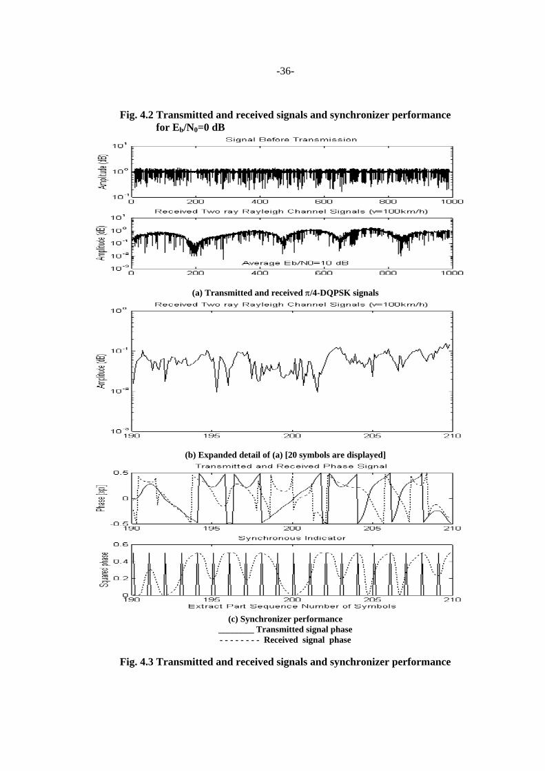
SIMULATION RESULTS AND DISCUSSION 4.1 Introduction A synchronization model based on multirate techniques is presented here by establishing a phase adjuster and searching processor for a synchronizer. The phase adjuster employed to diminish phase distortion of the fading channel, and searching processor is a unit that can extract symbol time instants by means of comparing the SIQ signal phase with the reference phase. A bit error rate (BER) simulation was carried out for evaluating DCM system performance using MATLAB. Each simulation was conducted over 100 frames of data and averaged over three independent runs. 4.2 Simulation Results The performance of the synchronizer in fading channel is illustrated in Fig. 4.1, 4.2 and 4.3. From these figures, it is observed that the phase distortion and AWGN have appreciable influence to received signal. It can also be seen that after the phase adjuster, fading is diminished, and hence, SIQ signal phase remains the main features of π/4-DQPSK signal, as described in section 3.1. With the help of the training sequence and smoothing filter, synchronization can be achieved even if the transmitted signal is buried in noise. Even though the output data from the detector may contain a lot of errors, the received signal can be synchronized. Two rays channel model is used to analyze synchronization performance. In Fig. 4.1, since Eb/N0 is high enough for synchronization, i.e., the received signal phase keeps the main characteristics of π/4-DQPSK signal, so that the synchronization can be established within training sequence (acquisition) and achieved during data transmission (tracking). While in Fig. 4.2, with Eb/N0 equal to 0dB, the received signal is distorted by AWGN seriously, even the acquisition can be accomplished within training sequence, it becomes more difficult to track the adequate timing instant. In that case, estimated timing instant will be used for synchronization of data sequence and hence more timing errors may appear. Delay has no significant influence on synchronization, and it can be seen from Fig. 4.3. In this figure, Eb/N0 is chosen as 10dB, therefore the received signal can be recognized as π/4-DQPSK signal even with delay, and both acquisition and tracking can be achieved. However, the delay induced ISI is significant and the

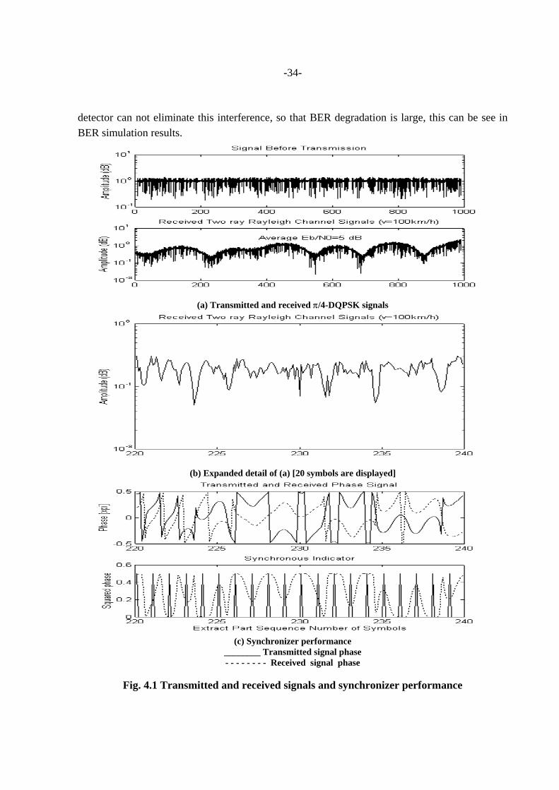
-34-

detector can not eliminate this interference, so that BER degradation is large, this can be see in BER simulation results.

(a) Transmitted and received π/4-DQPSK signals

(b) Expanded detail of (a) [20 symbols are displayed]

(c) Synchronizer performance

________ Transmitted signal phase - - - - - - - - Received signal phase

Fig. 4.1 Transmitted and received signals and synchronizer performance

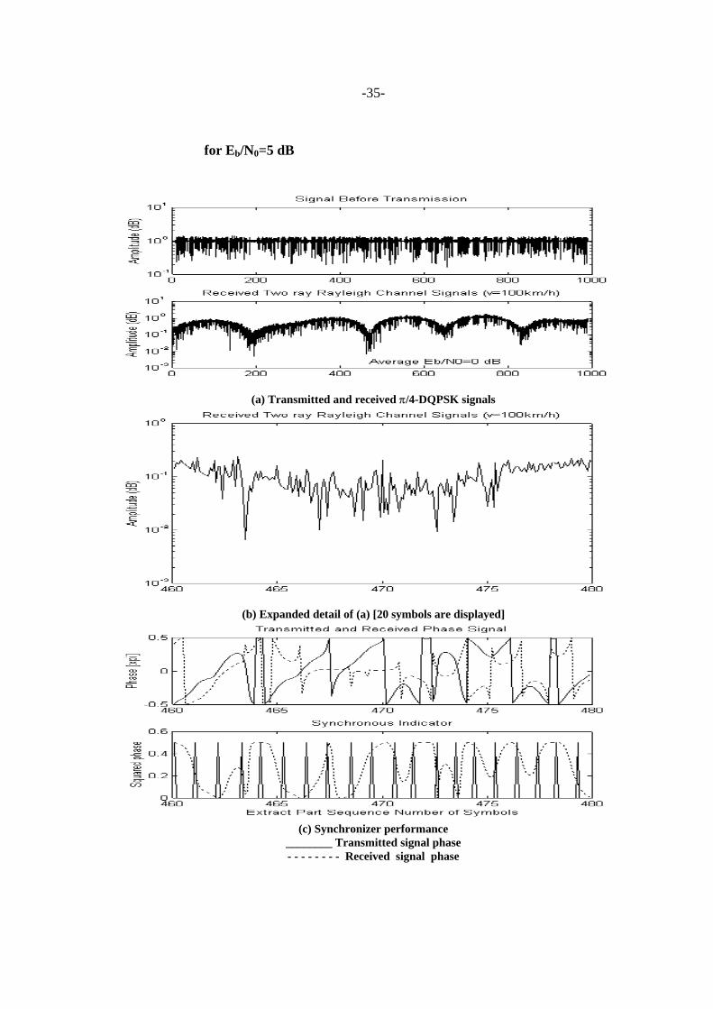
-35-

for Eb/N0=5 dB

(a) Transmitted and received π/4-DQPSK signals

(b) Expanded detail of (a) [20 symbols are displayed]

(c) Synchronizer performance

________ Transmitted signal phase - - - - - - - - Received signal phase

-36-

Fig. 4.2 Transmitted and received signals and synchronizer performance for Eb/N0=0 dB

(a) Transmitted and received π/4-DQPSK signals

(b) Expanded detail of (a) [20 symbols are displayed]

(c) Synchronizer performance

________ Transmitted signal phase - - - - - - - - Received signal phase

Fig. 4.3 Transmitted and received signals and synchronizer performance

-37-

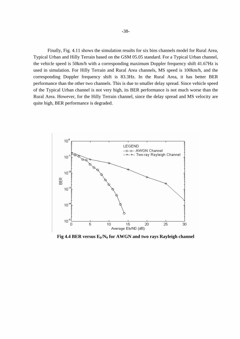
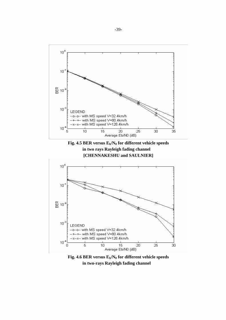
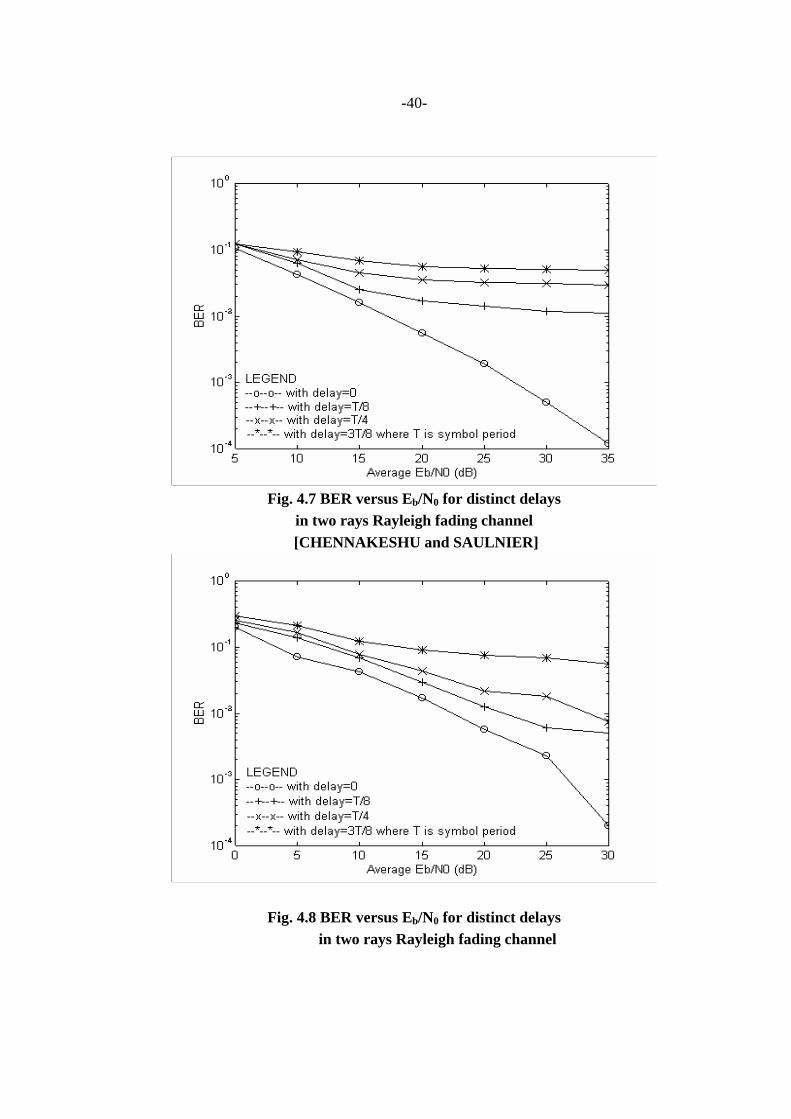
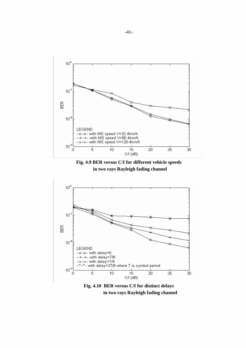
for Eb/N0=10 dB with delay τ=15.432µs Figure 4.4 illustrates the simulation results of BER versus Eb/N0 for an AWGN and two rays Rayleigh fading channel. Eb/N0 change from 0dB to 30dB are selected for BER simulation. This figure also gives the BER performance of the DCM system over AWGN channel. Compare obtained results in Figs. 4.6 and 4.8 with Figs. 4.5 and 4.7 which is given by CHENNAKESHU and SAULNIER (1993), the simulation results obtained in this thesis are similar to the Figs. 4.5 and 4.7. However, these two given figures are suitable for moderate frame length, it means that the transmission data frame can not be too long, because the synchronization is achieved within the preamble and they have no tracking ability. Figure 4.6 illustrates BER versus Eb/N0, for different vehicle speeds of 32.4km/h, 80.4km/h and 128.4km/h and carrier frequency of 900MHz, the corresponding maximum Doppler frequencies are 27Hz, 67Hz and 107Hz, respectively. If the vehicle speed is less than 80km/h, the degradation is smaller and acceptable; if the vehicle speed is higher than 100km/h, the degradation is observed to be high. Because the symbol timing algorithm given in Eq. 3.19 and 3.21 is based on the assumption that channel-induced fading can not be too fast, and the phase distortion changes a little for succeeding symbols. Once the vehicle speed exceeds a threshold and creates bigger phase distortion changes for continuous symbols, the BER performance may become worse. Figure 4.8 illustrates the BER degradation with distinct delays for two rays Rayleigh channel. A vehicle speed of 32.4km/h is assumed for the simulation. In Fig. 4.8, delays are 0, T/8=5.144µs, T/4=10.288µs and 3T/8=15.432µs. From this figure, it is seen that the delay must be less than 1/8 (≈5µs) of the symbol period for an acceptable BER performance. Because when delay becomes larger, the channel induced ISI increased significantly. As a result, the detector does not work properly due to larger delays. We may therefore need equalizer to achieve good BER performance with larger delays. Figure 4.9 and 4.10 show performance results for cochannel interference. In order to see the practical influence of cochannel interference, an Eb/N0 is chosen as 20 dB for CCI simulation. To obtain these results, a second π/4-DQPSK signal was employed as an interference. Fig. 4.9 gives BER performance as a function of C/I for distinct vehicle speed. From Fig. 4.10 the BER performance degrades rapidly for increasing delay with the consideration of CCI. Since the BER performance shown in Fig. 4.8 indicates an irreducible degradation for large delay, the BER performance for CCI with delay can not be improved.

-38-

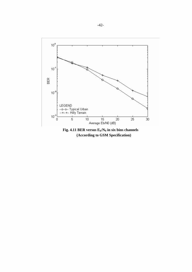
Finally, Fig. 4.11 shows the simulation results for six bins channels model for Rural Area, Typical Urban and Hilly Terrain based on the GSM 05.05 standard. For a Typical Urban channel, the vehicle speed is 50km/h with a corresponding maximum Doppler frequency shift 41.67Hz is used in simulation. For Hilly Terrain and Rural Area channels, MS speed is 100km/h, and the corresponding Doppler frequency shift is 83.3Hz. In the Rural Area, it has better BER performance than the other two channels. This is due to smaller delay spread. Since vehicle speed of the Typical Urban channel is not very high, its BER performance is not much worse than the Rural Area. However, for the Hilly Terrain channel, since the delay spread and MS velocity are quite high, BER performance is degraded.

Fig 4.4 BER versus Eb/N0 for AWGN and two rays Rayleigh channel

-39-

Fig. 4.5 BER versus Eb/N0 for different vehicle speeds

in two rays Rayleigh fading channel [CHENNAKESHU and SAULNIER]

Fig. 4.6 BER versus Eb/N0 for different vehicle speeds

in two-rays Rayleigh fading channel

-40-

Fig. 4.7 BER versus Eb/N0 for distinct delays

in two rays Rayleigh fading channel [CHENNAKESHU and SAULNIER]

Fig. 4.8 BER versus Eb/N0 for distinct delays in two rays Rayleigh fading channel

-41-

Fig. 4.9 BER versus C/I for different vehicle speeds

in two rays Rayleigh fading channel

Fig. 4.10 BER versus C/I for distinct delays

in two rays Rayleigh fading channel

-42-

Fig. 4.11 BER versus Eb/N0 in six bins channels

(According to GSM Specification)

-43-

CHAPTER V

CONCLUSIONS AND RECOMMENDATIONS 5.1 Conclusions This thesis investigated an multirate technique for timing recovery with the mobile radio channel. A π/4-shifted-DQPSK system based on North American IS-54 specifications is assumed. The proposed timing algorithm performance under the condition of deep fading and the high values of Eb/N0 is investigated. The results of BER performance in frequency-selective fading channel models such as two rays, typical urban, rural area and hilly terrain are presented and compared. In the two rays model, the influence of delay, vehicle speed and cochannel interference are studied. The timing algorithm has both acquisition and tracking ability during the whole data frame. Acquisition can be achieved by using training sequences. The tracking capability depends on the characteristics of the received signal. If the received signal can still be identified as π/4-DQPSK signal, i.e., SIQ signal phase value be shifted ±π/4 for consecutive symbols, the tracking process can work properly. The synchronizer can not track the transition in data sequence, if the effect of noise makes the received signal lost its features. In that case, an estimated timing instant is applied after acquisition and hence it may produce timing errors. Delay, which cause ISI, has no significant effect on synchronization because the received signal with delay still have the same characteristics of π/4-DQPSK signal, therefore the tracking can be achieved. As delay spread becomes bigger, BER degradation is increased because a large delay spread induces large ISI to communication systems. The experimental results show that without an equalizer, the acceptable BER performance is restricted within delay less than 5µs. Therefore, to reduce BER degradation in frequency-selective fading channels, an adaptive equalizer is suggested. (e.g., DFE, Viterbi Equalizer, etc.) High vehicle speed causes fast fading, and the changes of phase distortion between two consecutive symbols become faster as well. Since the synchronization algorithm, both acquisition and tracking, is based on the assumption that phase distortion changes remain constant for succeeding transmitted symbols. The BER degradation is irreducible for high MS velocity. However, within normal vehicle speed ranges (e.g., less than 200km/h) and without large delay, this assumption can be satisfied and BER performance is friendly.

-44-

The inherent advantage of the multirate techniques model is that it can be fulfilled in a totally digital environment. As a result, there are no feedback loops needed to control the analog device ⎯ sampler, hence the complexity design task of combining digital and analog can be reduced by separating them into two independent parts. However, in doing that, a high sampling rate sampler is desired, and more computations are thus necessary. Fortunately, as mature VLSI techniques are available and computer industry is still under development, DSP techniques can be easily used, and therefore multirate techniques are feasible for real-time communications systems. The results obtained in this paper is useful in the design of a fully digital receiver for TDMA second generation cellular systems currently under development in North American and Japan. 5.2 Recommendations for Future Research (1) In doing the research to improve the BER performance for a fading channel, diversity techniques are preferred choice to eliminate the corruption of deep fading. The diversity method can smooth out the fast fading and reduce the variations in the received signal to the level of slow fading. This method should be studied in further research. (2) Since no equalizer has yet been used in this simulation system, and the detector is easily disturbed with interference or delay, future research should look at how an adaptive equalizer can be applied to this system for the purpose of attenuating ISI.

-45-

REFERENCES AGHVAMI, A.H. (1993), Digital Modulation Techniques for Mobile and Personal Communication Systems, Electronics & communication Engineering Journal, Vol. 5, No. 3, pp. 125-132. ARMSTRONG, J. (1991), Symbol Synchronization Using Baud-Rate Sampling and Data- Sequence-Dependent Signal Processing, IEEE Transactions on Communications, Vol. COM-39, No. 1, pp. 127-132. ARMSTRONG, J. and STRICKLAND, D. (1993), Symbol Synchronization Using Signal Samples and Interpolation, IEEE Transactions on Communications, Vol. 41, No. 2, pp. 318-321. BRANDAO, A.L., LOPES, L.B. and MCLERNON, D.C. (1994), Method for Timing Recovery in Presence of Multipath Delay and Cochannel Interference, Electronics Letters, Vol. 30, No. 13, pp. 1028-1029. BUCKET, K. and MOENECLAEY, M. (1994), The Effect of Interpolation on the BER Performance of Narrowband BPSK and (O)QPSK on Rician-Fading Channels, IEEE Transactions on Communications, Vol. 42, No. 11, pp. 2929-2933. CARLSON, A. B. (1986), Communication Systems, McGraw-Hill. CHENNAKESHU, S. and SAULNIER, G.J. (1993), Differential Detection of π/4-Shifted DQPSK for Digital Cellular Radio, IEEE Transactions on Vehicular Technology, Vol. 42, No. 1, pp. 46-57. COWLEY, W.G. and SABEL, L.P. (1994), The Performance of Two Symbol Timing Recovery Algorithms for PSK Demodulators, IEEE Transactions on Communications, Vol.42, No. 6, pp. 2345-2355. D’ANDREA, N.A. and LUISE, M. (1993), Design and Analysis of a Jitter-Free Clock Recovery Scheme for QAM System, IEEE Transactions on Communications, Vol.41, No.9, pp. 1296-1299.

-46-

ERUP, L., GARDNER, F.M. and HARRIS, R.A. (1993), Interpolation in Digital Modems⎯Part II: Implementation and Performance, IEEE Transactions on Communications, Vol. 41, No. 6, pp. 998-1008. FEHER, K. (1991), MODEMS for Emerging Digital Cellular-Mobile Radio System, IEEE Transactions on Vehicular Technology, Vol. 40, No. 2, pp. 355-365. FINES, P. and AGHVAMI, A.H. (1991), Fully Digital M-ary PSK and M-ary QAM Demodulators for Land Mobile Satellite Communications, Electronics & communication Engineering Journal, Vol. 3, No. 6, pp. 291-298. GARDNER, F.M. (1986), A BPSK/QPSK Timing-Error Detector for Sampled Receivers, IEEE Transactions on Communications, Vol. 34, No. 5, pp. 423-429. GARDNER, F.M. (1993), Interpolation in Digital Modems⎯Part I: Fundamentals, IEEE Transactions on Communications, Vol. 41, No. 3, pp. 501-507. GARDNER, F.M. and LINDSEY W.C. (1980), Guest Editorial Special Issue on Synchronization, IEEE Transactions on Communications, Vol. 28, No.8, pp. 1105-1106. HAYKIN, S. (1988), Digital Communications, John Wiley & Sons. MÄKELÄINEN, K. (1995), Cellular Mobile Systems, Telecommunication Program, School of Advance Technologies, Asian Institute of Technology. MUELLER, K.H. and MÜLLER, M. (1976), Timing Recovery in Digital Synchronous Data Receivers, IEEE Transactions on Communications, Vol. COM-24, No. 5, pp. 516-531. NG, C.S., TJHUNG, T.T., ADACHI, F. and LYE, K.M. (1993), On the Error Rates of Differentially Detected Narrowband π/4-DQPSK in Rayleigh Fading and Gaussian Noise, IEEE Transactions on Vehicular Technology, Vol. 42, No. 3, pp. 259-265. OERDER, M. (1987), Derivation of Gardner’s Timing-Error Detector from the Maximum Likelihood Principle, IEEE Transactions on Communications, Vol. 35, No. 6, pp. 684-685. PROAKIS, J.G. (1983), Digital Communications, McGraw-Hill.

-47-

SCHAFER, R.W. and RABINER, L.R. (1973), A Digital Signal Processing Approach to Interpolation, Proceedings of the IEEE, Vol.61, No. 6, pp. 692-702. STEELE, R (1992), Mobile Radio Communications, Pentech Press. WANG, Z., JULLIEN, G.A. and MILLER, W.C. (1993), Interpolation Using the Discrete Sine Transform with Increased Accuracy, Electronics Letters, Vol. 29, No. 22, pp. 1918-1920. WATKIN, L.R. and BIHAN, J.Le (1994), Fast Accurate Interpolation with B-Spline Scaling Functions, Electronics Letters, Vol. 30, No. 13, pp. 1024-1025. WEI, C.H. and CHEN, W.J. (1994), Digital Tanlock Loop for Tracking π/4-DQPSK Signal in Digital Cellular Radio, IEEE Transactions on Vehicular Technology, Vol. 43, No. 3, pp. 474-479.

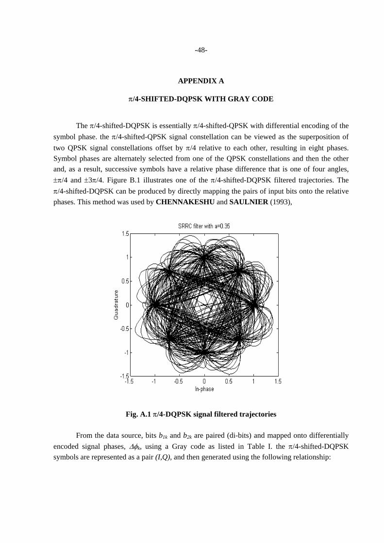
-48-

APPENDIX A

π/4-SHIFTED-DQPSK WITH GRAY CODE The π/4-shifted-DQPSK is essentially π/4-shifted-QPSK with differential encoding of the symbol phase. the π/4-shifted-QPSK signal constellation can be viewed as the superposition of two QPSK signal constellations offset by π/4 relative to each other, resulting in eight phases. Symbol phases are alternately selected from one of the QPSK constellations and then the other and, as a result, successive symbols have a relative phase difference that is one of four angles, ±π/4 and ±3π/4. Figure B.1 illustrates one of the π/4-shifted-DQPSK filtered trajectories. The π/4-shifted-DQPSK can be produced by directly mapping the pairs of input bits onto the relative phases. This method was used by CHENNAKESHU and SAULNIER (1993),

Fig. A.1 π/4-DQPSK signal filtered trajectories From the data source, bits b1k and b2k are paired (di-bits) and mapped onto differentially encoded signal phases, ∆φk, using a Gray code as listed in Table I. the π/4-shifted-DQPSK symbols are represented as a pair (I,Q), and then generated using the following relationship:

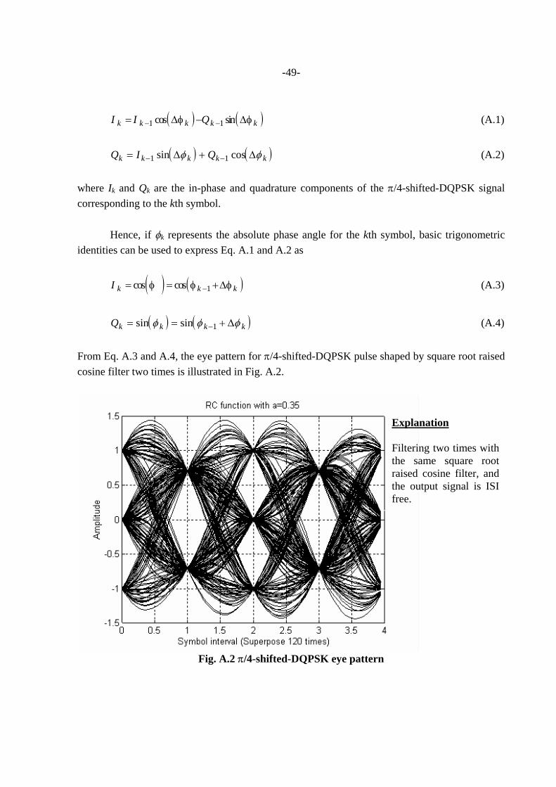
-49-

( ) ( )I I Qk k k k k= −− −1 1cos sin∆φ ∆φ (A.1) ( ) ( )Q I Qk k k k k= +− −1 1sin cos∆ ∆φ φ (A.2) where Ik and Qk are the in-phase and quadrature components of the π/4-shifted-DQPSK signal corresponding to the kth symbol. Hence, if φk represents the absolute phase angle for the kth symbol, basic trigonometric identities can be used to express Eq. A.1 and A.2 as

( ) ( )I k k k= = +−cos cosφ φ 1 ∆φ (A.3)

( ) ( )Qk k k k= = +−sin sinφ φ φ1 ∆ (A.4) From Eq. A.3 and A.4, the eye pattern for π/4-shifted-DQPSK pulse shaped by square root raised cosine filter two times is illustrated in Fig. A.2.

Fig. A.2 π/4-shifted-DQPSK eye pattern

Explanation Filtering two times with the same square root raised cosine filter, and the output signal is ISI free.

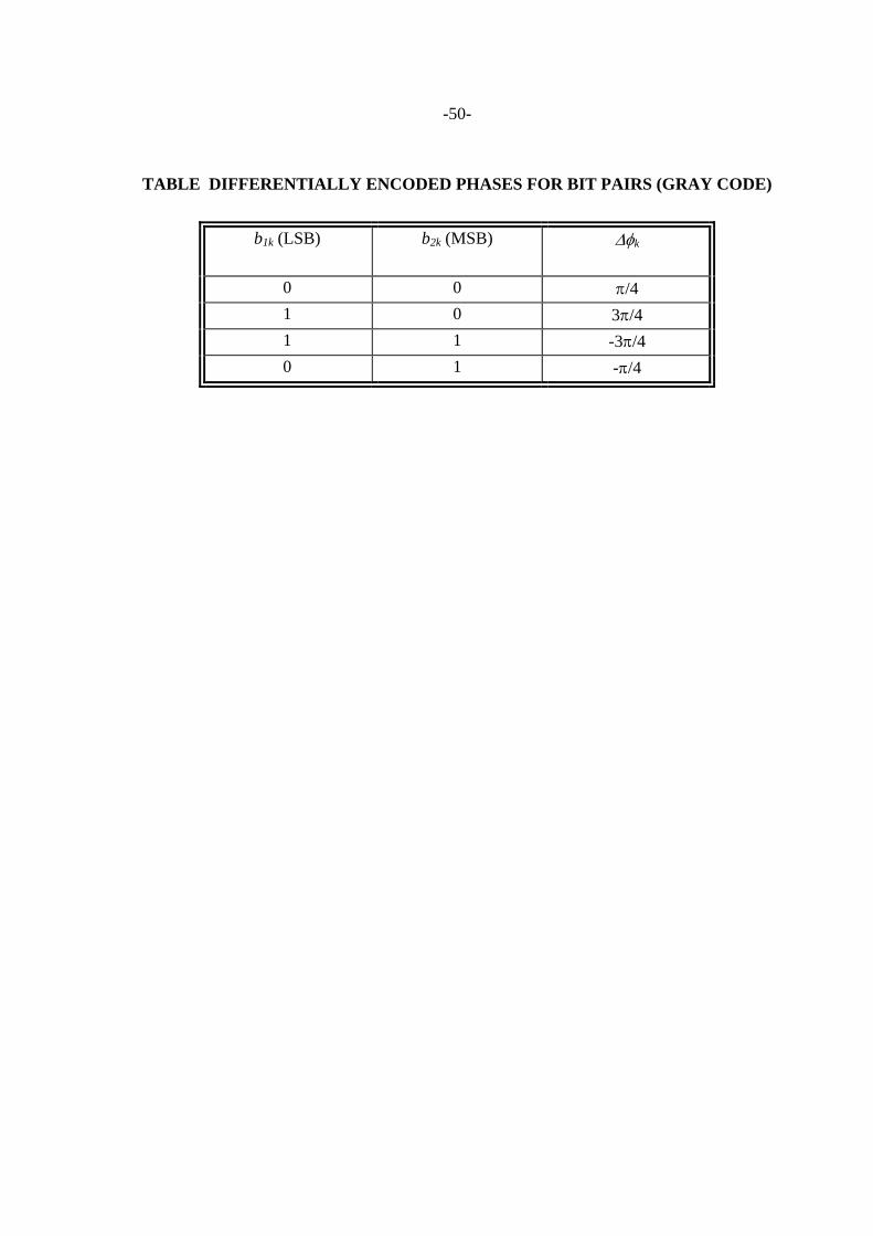
-50-

TABLE DIFFERENTIALLY ENCODED PHASES FOR BIT PAIRS (GRAY CODE)

b1k (LSB)

b2k (MSB) ∆φk

0 0 π/4 1 0 3π/4 1 1 -3π/4 0 1 -π/4

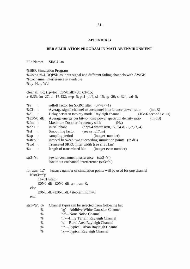
-51-

APPENDIX B

BER SIMULATION PROGRAM IN MATLAB ENVIRONMENT

File Name: SIMU1.m %BER Simulation Program %Using pi/4-DQPSK as input signal and different fading channels with AWGN %Cochannel interference is available %by Han, Wei clear all; tic; t_p=toc; E0N0_dB=60; CI=15; a=0.35; fm=27; dl=15.432; step=5; ph1=pi/4; sf=15; sp=20; x=324; wd=5; %a : rolloff factor for SRRC filter (0<=a<=1) %CI : Average signal channel to cochannel interference power ratio (in dB) %dl : Delay between two ray model Rayleigh channel (10e-6 second i.e. us) %E0N0_dB: Average energy per bit-to-noise power spectrum density ratio (in dB) %fm : Maximum Doppler frequency shift (Hz) %ph1 : initial phase (n*pi/4 where n=0,1,2,3,4 & -1,-2,-3,-4) %sf : Smoothing factor (see sync17.m) %sp : sampling period (integer number) %step : interval between two succeeding simulation points (in dB) %wd : Truncated SRRC filter width (see srrcd1.m) %x : length of transmitted bits (integer even number) str3='y'; %with cochannel interference (str3='y') %without cochannel interference (str3='n') for csnr=1:7 %csnr : number of simulation points will be used for one channel if str3=='y' CI=CI+step; E0N0_dB=E0N0_dB;err_num=0; else E0N0_dB=E0N0_dB+step;err_num=0; end str1='tr'; % Channel types can be selected from following list % 'ag'---Additive White Gaussian Channel % 'ne'---None Noise Channel % 'hi'---Hilly Terrain Rayleigh Channel % 'ru'---Rural Area Rayleigh Channel % 'ur'---Typical Urban Rayleigh Channel % 'ry'---Typical Rayleigh Channel

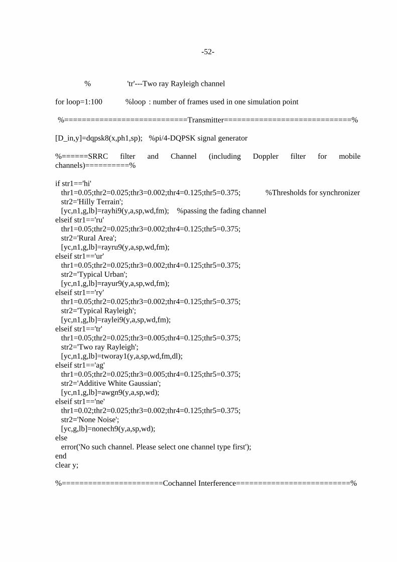
-52-

% 'tr'---Two ray Rayleigh channel for loop=1:100 %loop : number of frames used in one simulation point

%============================Transmitter=============================%

[D_in,y]=dqpsk8(x,ph1,sp); %pi/4-DQPSK signal generator %======SRRC filter and Channel (including Doppler filter for mobile channels)==========% if str1=='hi' thr1=0.05;thr2=0.025;thr3=0.002;thr4=0.125;thr5=0.375; %Thresholds for synchronizer str2='Hilly Terrain'; [yc,n1,g,lb]=rayhi9(y,a,sp,wd,fm); %passing the fading channel elseif str1=='ru' thr1=0.05;thr2=0.025;thr3=0.002;thr4=0.125;thr5=0.375; str2='Rural Area'; [yc,n1,g,lb]=rayru9(y,a,sp,wd,fm); elseif str1=='ur' thr1=0.05;thr2=0.025;thr3=0.002;thr4=0.125;thr5=0.375; str2='Typical Urban'; [yc,n1,g,lb]=rayur9(y,a,sp,wd,fm); elseif str1=='ry' thr1=0.05;thr2=0.025;thr3=0.002;thr4=0.125;thr5=0.375; str2='Typical Rayleigh'; [yc,n1,g,lb]=raylei9(y,a,sp,wd,fm); elseif str1=='tr' thr1=0.05;thr2=0.025;thr3=0.005;thr4=0.125;thr5=0.375; str2='Two ray Rayleigh'; [yc,n1,g,lb]=tworay1(y,a,sp,wd,fm,dl); elseif str1=='ag' thr1=0.05;thr2=0.025;thr3=0.005;thr4=0.125;thr5=0.375; str2='Additive White Gaussian'; [yc,n1,g,lb]=awgn9(y,a,sp,wd); elseif str1=='ne' thr1=0.02;thr2=0.025;thr3=0.002;thr4=0.125;thr5=0.375; str2='None Noise'; [yc,g,lb]=nonech9(y,a,sp,wd); else error('No such channel. Please select one channel type first'); end clear y; %=======================Cochannel Interference==========================%

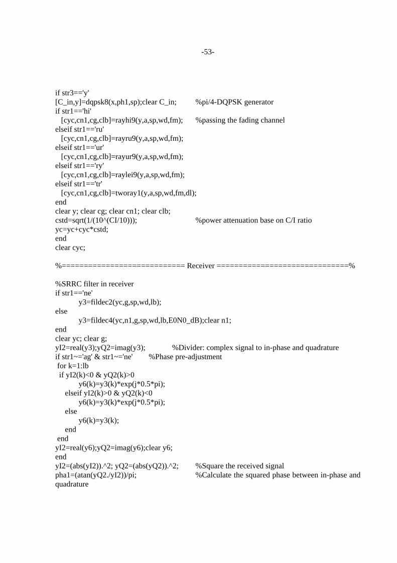
-53-

if str3=='y' [C_in,y]=dqpsk8(x,ph1,sp);clear C_in; %pi/4-DQPSK generator if str1=='hi' [cyc,cn1,cg,clb]=rayhi9(y,a,sp,wd,fm); %passing the fading channel elseif str1=='ru' [cyc,cn1,cg,clb]=rayru9(y,a,sp,wd,fm); elseif str1=='ur' [cyc,cn1,cg,clb]=rayur9(y,a,sp,wd,fm); elseif str1=='ry' [cyc,cn1,cg,clb]=raylei9(y,a,sp,wd,fm); elseif str1=='tr' [cyc,cn1,cg,clb]=tworay1(y,a,sp,wd,fm,dl); end clear y; clear cg; clear cn1; clear clb; cstd=sqrt(1/(10^(CI/10))); %power attenuation base on C/I ratio yc=yc+cyc*cstd; end clear cyc; %============================ Receiver ==============================% %SRRC filter in receiver if str1=='ne' y3=fildec2(yc,g,sp,wd,lb); else y3=fildec4(yc,n1,g,sp,wd,lb,E0N0_dB);clear n1; end clear yc; clear g; yI2=real(y3);yQ2=imag(y3); %Divider: complex signal to in-phase and quadrature if str1~='ag' & str1~='ne' %Phase pre-adjustment for k=1:lb if yI2(k)<0 & yQ2(k)>0 y6(k)=y3(k)*exp(j*0.5*pi); elseif yI2(k)>0 & yQ2(k)<0 y6(k)=y3(k)*exp(j*0.5*pi); else y6(k)=y3(k); end end yI2=real(y6);yQ2=imag(y6);clear y6; end yI2=(abs(yI2)).^2; yQ2=(abs(yQ2)).^2; %Square the received signal pha1=(atan(yQ2./yI2))/pi; %Calculate the squared phase between in-phase and quadrature

-54-

clear yI2;clear yQ2; %==========================Synchronizor==============================% [s_point,A]=sync17(pha1,sp,sf,thr1,thr2,thr3,thr4,thr5);clear pha1; %============================Decimater==============================% y5=seldec2(y3,s_point,lb,A); clear s_point; clear lb; clear y3; %============================Detector===============================% dph=detect2(y5,A,ph1); %Differential Detector D_out=dataout1(dph); clear y5; clear dph; clear A; %========================== Error protector ============================% ld=length(D_out); if ld~=length(D_in) if loop>1 loop=loop-1; else loop=1; end else DF=D_in-D_out; err_num=length(find(DF(3:ld)))+err_num; %err_num is the detected error end clear DF;clear D_in; clear D_out; clear ld; %======================BER analysis and Results saving======================% if toc>=t_p+600 save c:\MATLAB\hwth\lib\buff1 err_num loop str1 E0N0_dB CI str3 t_p=toc; end end time=rem(toc,3600); time=[fix(toc/3600) fix(time/60) fix(rem(time,60))] ld=(x+14)*loop; BER(csnr)=err_num/ld if str3=='y' BER_dB(1,csnr)=CI; else

-55-

BER_dB(1,csnr)=E0N0_dB; end BER_dB(2,csnr)=10*log10(BER(csnr)) save c:\MATLAB\hwth\lib\berag3 BER BER_dB err_num loop str1 clo=clock;current_clock=clo(1:5) end Channel_type=str2 ***************************************************************************** File Name: DQPSK8.m %built pi/4-shifted-DQPSK symbol (transmitted symbol) function [b,y]=dqpsk8(x,phase12,sp); %b : transmitted binary data sequence %phase12: initial phase (n*pi/4 where n=0,1,2,3,4 & -1,-2,-3,-4) %sp : sampling period (integer number) %x : symbol length (integer number) %y : transmitted complex signal b=[zeros(1,x)]; e=1:1:x; for e=1:x, %built random binary data c=randn(1); if c<0.5 b(e)=0; else b(e)=1; end end b=[zeros(1,16) b]; x=x+16; %add training sequency del_const=phase12; i=1; %initial phase for Tx-signal is the last phase of training for n=1:x/2, %built the Gray encoding if b(i)==0 if b(i+1)==0 delphase(n)=pi/4+del_const; end if b(i+1)==1 delphase(n)=-pi/4+del_const; end end if b(i)==1 if b(i+1)==0 delphase(n)=3*pi/4+del_const;

-56-

end if b(i+1)==1 delphase(n)=-3*pi/4+del_const; end end %built impulse response Tx-signal base on sample duration sp% y((n-1)*sp+1)=exp(j*delphase(n)); for t=(n-1)*sp+2:n*sp y(t)=0; end del_const=delphase(n); i=i+2; end **************************************************************************** File Name: RAYHI9.m %Rayleigh Fading Channel with Doppler Filter for Hilly Area function [outI,n13,g1,lb]=rayhi9(inputI,a,sp,wd,fm) %g1 : main ray SRRC filter coefficients %inputI : input complex signal %lb : length of transmitted signal (symbols) %n13 : channel induced AWGN %outI : output complex signal of HT fading channel lb=length(inputI); %================ Generate SRRC filters with different delays ==================% [t1,g1]=srrcd1(sp,wd,0); [t2,g2]=srrcd1(sp,wd,0.1); [t3,g3]=srrcd1(sp,wd,0.3); [t4,g4]=srrcd1(sp,wd,0.5); [t5,g5]=srrcd1(sp,wd,15.0); [t6,g6]=srrcd1(sp,wd,17.2); %================== Filter the input signal in time domain =====================% I1=conv(g1,inputI); I1=I1(wd*sp+1:wd*sp+lb); I2=conv(g2,inputI); I2=I2(wd*sp+1:wd*sp+lb); I3=conv(g3,inputI); I3=I3(wd*sp+1:wd*sp+lb); I4=conv(g4,inputI); I4=I4(wd*sp+1:wd*sp+lb); I5=conv(g5,inputI); I5=I5(wd*sp+1:wd*sp+lb); I6=conv(g6,inputI); I6=I6(wd*sp+1:wd*sp+lb);

-57-

%=========== Generate White Gaussian Noise and filtered by Doppler filter ===========% load c:\MATLAB\hwth\lib\dopdata1; n=200; %coefficient of Doppler filter n1=dopfil3(lb,sp,fm,b,0.4549,n); n2=dopfil3(lb,sp,fm,b,0.4549,n); n3=dopfil3(lb,sp,fm,b,0.3828,n); n4=dopfil3(lb,sp,fm,b,0.3828,n); n5=dopfil3(lb,sp,fm,b,0.2710,n); n6=dopfil3(lb,sp,fm,b,0.2710,n); n7=dopfil3(lb,sp,fm,b,0.1918,n); n8=dopfil3(lb,sp,fm,b,0.1918,n); n9=dopfil3(lb,sp,fm,b,0.1811,n); n10=dopfil3(lb,sp,fm,b,0.1811,n); n11=dopfil3(lb,sp,fm,b,0.0593,n); n12=dopfil3(lb,sp,fm,b,0.0593,n); r1=n1+j*n2; r2=n3+j*n4; r3=n5+j*n6; r4=n7+j*n8; r5=n9+j*n10; r6=n11+j*n12; %================== Go through this Rayleigh fading channel =================% outI1=I1.*r1; outI2=I2.*r2; outI3=I3.*r3; outI4=I4.*r4; outI5=I5.*r5; outI6=I6.*r6; n13=awgn5(lb); %built AWGN outI=outI1+outI2+outI3+outI4+outI5+outI6; ****************************************************************************** File Name: SRRCD1.m %Set up SRRC filter's coefficient with delay %This program can be used for roll-off a=0.35 ONLY function [t,g]=srrcd1(sp,wd,td) %g : SRRC filter coefficient with delay %sp : sampling period %t : truncated timing duration %td : delay spread %wd : truncate width a=0.35; T=1; k=0; td=(td*1e-6)*24300; %transmission symbol rate is 24.3 KHz for t=-wd:1/sp:wd k=k+1; if t-td==0 g(k)=1-a+4*(a/pi); elseif t-td==T/(4*a) g(k)=a/sqrt(2)*((1+2/pi)*sin(pi/(4*a))+(1-2/pi)*cos(pi/(4*a))); else

-58-

g(k)=(sin(pi*(1-a)*(t-td)/T)+4*a*(t-td)/T*cos(pi*(1+a)*(t-td)/T))/(pi*(t-td)/T*(1-(4*a*(t-td)/T)^2)); end end t=-wd:1/sp:wd; ****************************************************************************** Files For Generate DOPDATA1.mat which is a MAT-file contains Doppler filter coefficient File Name: DOPPLER6.m %Built up Doppler filter's frequency response function [f,H]=doppler6(csp) %csp : sample period of frequency response for Doppler filter %f : normalized frequency %H : magnitude of Doppler frequency response fm=0.5; %maximum normalized Doppler frequency shift A=1;e=1; for f=0:1/csp:1 if f>=0.5 H(e)=0; else H(e)=sqrt(A./sqrt(1-(f/fm).^2)); end e=e+1; end f=0:1/csp:1; &&&&&&&&&&&&&&&&&&&&&&&&&&&&&&&&&&&&&&&&&&&&&&&&&&& File Name: DOPPLER7.m %Set up Doppler filter coefficient %Increase the input sampling rate of Doppler filter by compress the normalized max. Doppler frequency as much as %possible function [f,H1,mati,b]=doppler7(csp,m) %csp : sample period of frequency response for Doppler filter %H1 : magnitude of compressed frequency response

-59-

%m : compress factor n=1000; %filter order nf=2/m; mati=2*m; [f,H]=doppler6(csp); %frequency response e=1; for r=1:nf/csp:nf+1 H1((r-1)*(csp/nf)+1)=H(e); e=e+1; end for r=nf+1+(nf/csp):nf/csp:2 H1((r-1)*(csp/nf)+1)=0; end f=0:nf/csp:1; b=fir2(n,f,H1,kaiser(n+1,0.1102*(50-8.7))); %apply Kaiser window save c:\MATLAB\hwth\lib\dopdata2 b; %buffer the coefficients to MAT-file ************************************************************************** File Name: DOPFIL3.m %Generate white Gaussian noise and passing Doppler filter %Interpolation to symbol rate (designed for transmission bit rate equal to 48.6kbps) %limitation processing given the minimum computation burden function out=dopfil3(lb,sp,fm,b,std,n) %b : coefficient of Doppler filter %fm : maximum Doppler frequency shift %lb : input data length %n : Doppler filter order %sp : sampling period %std : standard deviation of AWGN generator fm=fix(fm); %==============================limitation==============================% lim_m7e=ceil(lb/sp); lim_m7b=10; lim_m6e=ceil(lim_m7e/9); lim_m6b=10; lim_m5e=ceil(lim_m6e/3); lim_m5b=10; lim_m4e=lim_m5e*4; lim_m4b=40; lim_m3e=lim_m4e*fm; lim_m3b=40*fm; lim_m2e=ceil(lim_m3e/10); lim_m2b=max([10,4*fm]);

-60-

lim_m1e=ceil(lim_m2e/10); lim_m1b=max([10,ceil(0.4*fm)]); lim_n2e=ceil(lim_m1e/9); lim_n2b=max([10,ceil(0.04*fm)]); lim_n1e=lim_n2e+n+10; lim_n1b=lim_n2b+n+10; %============================ Doppler filtering =========================% if lim_n1b<=lim_n1e t_num=lim_n1e; else t_num=lim_n1b; end noi1=std*awgn3(t_num); %Noise source with standard deviation noi2=filter(b,1,noi1);noi2=noi2(n+11:t_num); %==========Sampling rate vary by means of interpolation or decimation============% noi_m1=interp(noi2,9); if lim_m1b<=lim_m1e t_num=lim_m1e; else t_num=lim_m1b; end noi_m1=noi_m1(1:t_num); noi_m2=interp(noi_m1,10); if lim_m2b<=lim_m2e t_num=lim_m2e; else t_num=lim_m2b; end noi_m2=noi_m2(1:t_num); noi_m3=interp(noi_m2,10); if lim_m3b<=lim_m3e t_num=lim_m3e; else t_num=lim_m3b; end noi_m3=noi_m3(1:t_num); noi_m4=decimate(noi_m3,fm); if lim_m4b<=lim_m4e t_num=lim_m4e; else t_num=lim_m4b; end noi_m4=noi_m4(1:t_num); noi_m5=decimate(noi_m4,4); if lim_m5b<=lim_m5e t_num=lim_m5e; else t_num=lim_m5b;

-61-

end noi_m5=noi_m5(1:t_num); noi_m6=interp(noi_m5,3); if lim_m6b<=lim_m6e t_num=lim_m6e; else t_num=lim_m6b; end noi_m6=noi_m6(1:t_num); noi_m7=interp(noi_m6,9); if lim_m7b<=lim_m7e t_num=lim_m7e; else t_num=lim_m7b; end noi_m7=noi_m7(1:t_num); noi3=interp(noi_m7,sp); out=noi3(1:lb); ***************************************************************************** File Name: AWGN5.m %Built up Additive White Guassian Noise function n=awgn5(lb) n=randn(1,lb); ***************************************************************************** Other channel program have the similar structure as RAYHI9.m, therefore, we doesn’t list them here. ***************************************************************************** File Name: FILDEC4.m %The data filter(SRRC) in decimator and AWGN power adjusted function outI=fildec4(inputI,n1,g,sp,wd,lb,E0N0_dB) std=sqrt(1/(10^(E0N0_dB/10))); n1=conv(g,n1)/sp; %convolution with AWGN n1=5*std*n1(wd*sp+1:wd*sp+lb); %power adjustment outI=conv(g,inputI)/sp; outI=outI(wd*sp+1:wd*sp+lb);outI=outI+n1; *************************************************************************** File Name: SYNC17.m

-62-

%This program be used for identify the synchronous point from input phase signals %input is the squared phase values %thrX are the different thresholds %Phase offset compensation function [s_point,A]=sync17(input,sp,sf,thr1,thr2,thr3,thr4,thr5) %A : number of synchronous point %s_point: synchronous point vector %sf : smoothing factor Data_length=length(input); Data_range=1; %Initial the start point s_point=[]; %Initial matrix mid_point=ceil(sp/2); lim=fix(mid_point/sf); flag=[]; flag1=[]; pha_off=(0.5-input(1))*pi; perpha=0.25; while Data_range<=Data_length-sp wind=input(Data_range:Data_range+sp-1); corr=exp(j*pha_off); c_result=exp(j*wind*pi).*corr; wind=atan(imag(c_result)./real(c_result))./pi; for k=1:sp-1 if wind(k)>0.5 wind(k)=1-wind(k); elseif wind(k)<0 wind(k)=-wind(k); else wind(k)=wind(k); end end dif_1=0.5-wind; Min_1=min(dif_1(find(dif_1<=thr1))); Min_0=min(wind(find(wind<=thr1))); shif=[];shifa=[];dalter=[]; %==================Identify phase position for S2 section ====================% if flag~=0.5 if isempty(Min_1)~=1 shif=find(dif_1==Min_1); [shifa,df]=select2(shif,mid_point); if isempty(s_point)~=1 %Smoothing if abs(df)>lim if df>0 df=lim; shifa=mid_point+lim; elseif df<0 df=-lim; shifa=mid_point-lim; end end end

-63-

s_point=[s_point Data_range-1+shifa];flag=0.5;flag1=[flag1,flag]; sm_off=input(Data_range-1+shifa)-perpha; %Phase correction perpha=input(Data_range-1+shifa); if sm_off>0 off=sm_off-0.25; else off=sm_off+0.25; end pha_off=(0.5-perpha+off)*pi; elseif isempty(Min_0)~=1 shif=find(wind==Min_0); [shifa,df]=select2(shif,mid_point); if isempty(s_point)~=1 %Smoothing if abs(df)>lim if df>0 df=lim; shifa=mid_point+lim; elseif df<0 df=-lim; shifa=mid_point-lim; end end end s_point=[s_point Data_range-1+shifa];flag=0.5;flag1=[flag1,flag]; sm_off=input(Data_range-1+shifa)-perpha; perpha=input(Data_range-1+shifa); if sm_off>0 off=sm_off-0.25; else off=sm_off+0.25; end pha_off=(1e-5-perpha+off)*pi; end end if isempty(shifa)==1 %================= Identify phase position for S4 section =====================% if flag~=0.25 range_limite=find(thr4<wind & wind<thr5); wind=wind(range_limite); dif_025=abs(wind-0.25); c_point=range_limite(find(dif_025<=thr2)); if isempty(c_point)~=1 [shifa,df]=select2(c_point,mid_point); if isempty(shifa)~=1 if isempty(s_point)~=1 %Smoothing if abs(df)>lim if df>0 df=lim; shifa=mid_point+lim; elseif df<0 df=-lim; shifa=mid_point-lim; end

-64-

end end s_point=[s_point Data_range-1+shifa];flag=0.25;flag1=[flag1,flag]; sm_off=input(Data_range-1+shifa)-perpha; perpha=input(Data_range-1+shifa); if sm_off>0 off=sm_off-0.25; else off=sm_off+0.25; end pha_off=(0.25-perpha+off)*pi; end end end end if isempty(shifa)==1 shifa=mid_point;df=0; s_point=[s_point Data_range-1+shifa];flag=0.1;flag1=[flag1,flag]; pha_off=pha_off; end %============================= Shifter ============================% Data_range=Data_range+df+sp; end A=length(s_point); &&&&&&&&&&&&&&&&&&&&&&&&&&&&&&&&&&&&&&&&&&&&&&&&& File Name: SELECT2.m %Choice an optimum output which is more close to mid_point (estimate point) function [out,dfa]=select2(input,mid_point) %dfa : shifting signal %mid_point: Estimate synchronous point which is located at middle of that detecting symbol df=input-mid_point; Min_df=find(abs(df)==min(abs(df))); out=input(Min_df); dfa=df(Min_df); if length(out)>1 out=out(1); dfa=dfa(1); end ****************************************************************************** File Name: SELDEC2.m

-65-

%Given the corresponding received signal values according to timing instant function out=seldec2(input,s_point,lb,A) e=1; for h=1:lb if e<=A if h==s_point(e) out(e)=input(h); e=e+1; end end end ***************************************************************************** File Name: DETECT2.m %Detect and given the differential phase value from received complex signal function dph=detect2(y,A,ph1) yI=real(y);yQ=imag(y); for m=1:A % range adjustment if yI(m)<0 pha(m)=atan(real(yQ(m)./yI(m)))/pi+1; else pha(m)=atan(real(yQ(m)./yI(m)))/pi; end end dph(1)=pha(1)-ph1; if dph(1)<-1 % mod 2*pi dph(1)=dph(1)+2; elseif dph(1)>1 dph(1)=dph(1)-2; end for n=2:A %differential dph(n)=pha(n)-pha(n-1); if dph(n)<-1 % mod 2*pi dph(n)=dph(n)+2; elseif dph(n)>1 dph(n)=dph(n)-2; end end *****************************************************************************

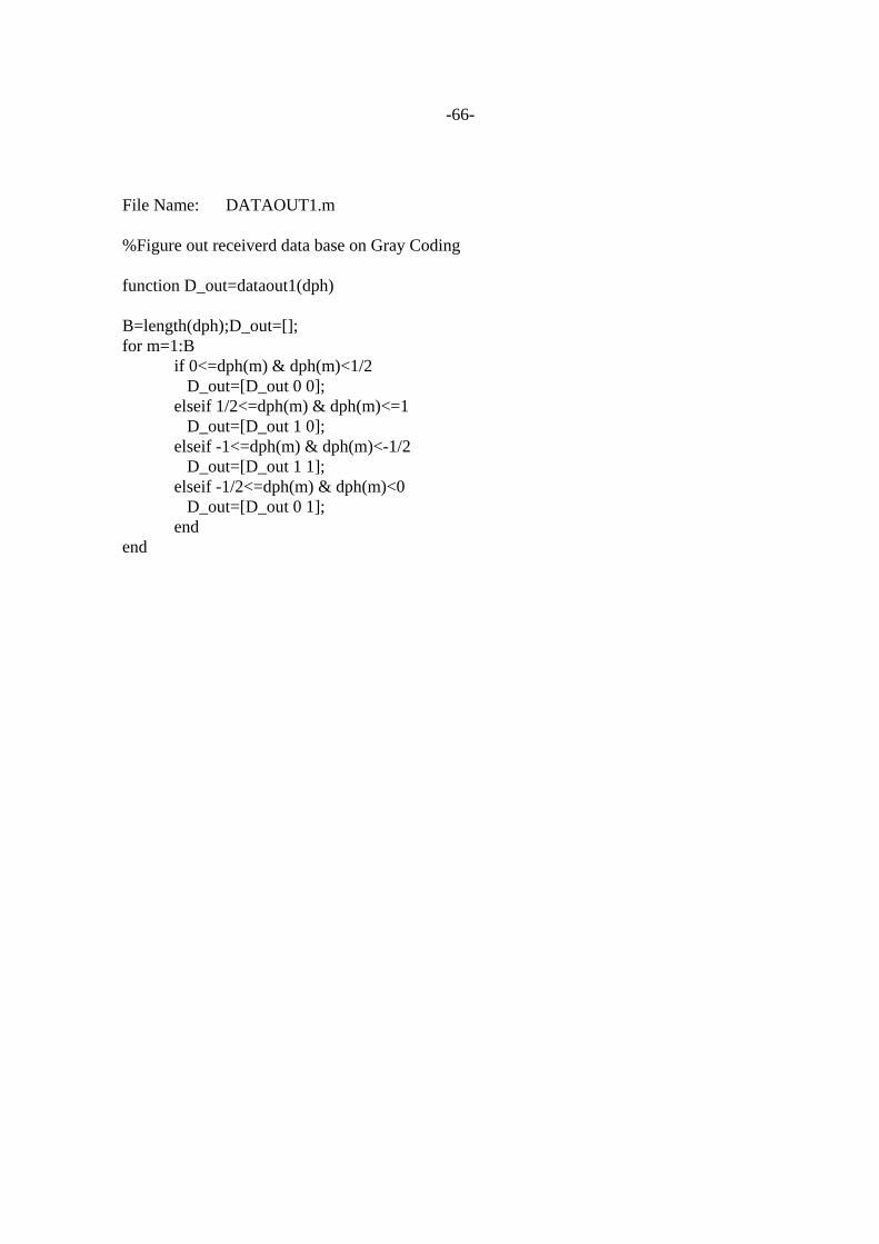
-66-

File Name: DATAOUT1.m %Figure out receiverd data base on Gray Coding function D_out=dataout1(dph) B=length(dph);D_out=[]; for m=1:B if 0<=dph(m) & dph(m)<1/2 D_out=[D_out 0 0]; elseif 1/2<=dph(m) & dph(m)<=1 D_out=[D_out 1 0]; elseif -1<=dph(m) & dph(m)<-1/2 D_out=[D_out 1 1]; elseif -1/2<=dph(m) & dph(m)<0 D_out=[D_out 0 1]; end end