Embed Size (px)
Citation preview

Loughborough UniversityInstitutional Repository
The architecture ofpneumatic regenerative
systems for the diesel engine
This item was submitted to Loughborough University's Institutional Repositoryby the/an author.
Additional Information:
• A Doctoral Thesis. Submitted in partial fulfilment of the requirementsfor the award of Doctor of Philosophy of Loughborough University.
Metadata Record: https://dspace.lboro.ac.uk/2134/21267
Publisher: c© Ran Bao
Rights: This work is made available according to the conditions of the Cre-ative Commons Attribution-NonCommercial-NoDerivatives 4.0 International(CC BY-NC-ND 4.0) licence. Full details of this licence are available at:https://creativecommons.org/licenses/by-nc-nd/4.0/
Please cite the published version.

THE ARCHITECTURE OF PNEUMATIC
REGENERATIVE SYSTEMS FOR THE
DIESEL ENGINE
by
Ran Bao
A Doctoral Thesis
Submitted in partial fulfilment of the requirements
for the award of
Doctor of Philosophy of Loughborough University
August 2015
© Ran Bao (2015)

CERTIFICATE OF ORIGINALITY
This is to certify that I am responsible for the work submitted in this thesis, that the
original work is my own except as specified in acknowledgments or in footnotes, and that
neither the thesis nor the original work contained therein has been submitted to this or
any other institution for a degree.
…………………………………………… (Signed)
…………………………………………… (Date)

i
ABSTRACT
For vehicles whose duty cycle is dominated by start-stop operation, fuel consumption
may be significantly improved by better management of the start-stop process.
Pneumatic hybrid technology represents one technology pathway to realise this goal.
Vehicle kinetic energy is converted to pneumatic energy by compressing air into air
tank(s) during the braking. The recovered air is reused to supply an air starter, or supply
energy to the air path in order to reduce turbo-lag.
This research aims to explore the concept and control of a novel pneumatic hybrid
powertrain for a city bus application to identify the potential for improvements in fuel
economy and drivability.
In order to support the investigation of energy management, system architecture and
control methodologies, two kinds of simulation models are created. Backward-facing
simulation models have been built using Simulink. Forward-facing models have been
developed in the GT-POWER and Simulink co-simulation.
After comparison, the fully controllable hybrid braking system is chosen to realize the
regenerative braking function. A number of architectures for managing a rapid energy
transfer into the powertrain to reduce turbo-lag have been investigated.
A city bus energy control strategy has been proposed to realize the Stop-Start Function,
Boost Function, and Regenerative Braking Function as well as the normal operations. An
optimisation study is conducted to identify the relationships between operating
parameters and respectively fuel consumption, performance and energy usage.
In conclusion, pneumatic hybrid technology can improve the city bus fuel economy by at
least 6% in a typical bus driving cycle, and reduce the engine brake torque response and
vehicle acceleration. Based on the findings, it can be learned that the pneumatic hybrid
technology offers a clear and low-cost alternative to the electric hybrid technology in
improving fuel economy and vehicle drivability.

ii
PUBLICATIONS
[1] Bao, R. and Stobart, R., "Design and Optimisation of the Propulsion Control Strategy
for a Pneumatic Hybrid City Bus," SAE Int. J. Alt. Power. 5(1):2016, doi:10.4271/2016-
01-1175.
[2] Bao, R. and Stobart, R., "Evaluating the Performance Improvement of Different
Pneumatic Hybrid Boost Systems and Their Ability to Reduce Turbo-Lag", SAE Technical
Paper 2015-01-1159, 2015, doi:10.4271/2015-01-1159.
[3] Bao, R. and Stobart, R., "Study on Optimisation of Regenerative Braking Control
Strategy in Heavy-Duty Diesel Engine City Bus using Pneumatic Hybrid Technology", SAE
Technical Paper 2014-01-1807, 2014, doi:10.4271/2014-01-1807.
[4] Bao, R. and Stobart, R., "Using Pneumatic Hybrid Technology to Reduce Fuel
Consumption and Eliminate Turbo-Lag", SAE Technical Paper 2013-01-1452, 2013,
doi:10.4271/2013-01-1452.
iii
ACKNOWLEDGEMENTS
This project was supported by the UK Engineering and Physical Sciences Research
Council (EPSRC) under grant reference EP/I00601X/1.
First of all, I would like to express my most gratitude to my supervisor, Professor Richard
Stobart for his guidance, encouragement and support throughout my PhD study at
Loughborough University.
I also would like to thank Professor Hua Zhao and members of the Centre for Advanced
Powertrain and Fuels Research (CAPF) at Brunel University London for sharing their
simulation models and Valuable feedbacks.
I am very grateful to the Loughborough colleagues for their thought-provoking
discussions, helpful comments and assistance of modelling work on my research, the
technicians at the Department of Aeronautical and Automotive Engineering for their great
professional help and support, and the engineers at Support Group in the Gamma
Technologies Inc. for their technical support of using GT-SUITE:
Farraen Mohd-Azmin, Rifqi Irzuan Abdul Jalal, Dr Thomas Steffen, Dr Dezong
Zhao, Gill Youngs, Bonnie Erdelyi-Betts, Rawinder Nottra, Robert Flint, David
Travis, Adrian Broster, Graham Smith, Drew Mason and Martin Coleman –
Loughborough University
Dr Guangyu Dong (former Loughborough colleague) - University of Brighton
Dr Bo Wang (former Loughborough colleague) - Romax Technology Limited
Joseph Wimmer, Christopher A. Contag and Mike Arnett - Gamma Technologies
Inc.
Finally, the greatest thank to my family for the support, understanding and
encouragement.

iv
CONTENTS
CERTIFICATE OF ORIGINALITY ii
ABSTRACT i
PUBLICATIONS ii
ACKNOWLEDGEMENTS iii
CONTENTS iv
List of Figures x
List of Tables xvii
Nomenclature xx
Latin Letters xx
Greek Symbols xxi
Subscripts and Superscripts xxi
Abbreviations xxii
CHAPTER 1 INTRODUCTION 1
1.1 Introduction and Outline of the Thesis 1
1.2 Background 4
1.3 Hybrid Vehicle 5
1.3.1 Hybrid Electric Vehicle 9
1.3.2 Hydraulic Hybrid Vehicle 12
1.3.3 Pneumatic Hybrid Vehicle 13

v
1.4 Research Aims and Objectives 15
1.5 Methodology and Software 16
1.6 Contributions to Knowledge 18
CHAPTER 2 LITERATURE REVIEW 19
2.1 Introduction 19
2.2 Compressed Air Vehicle History 19
2.3 The Review of Previous Research 21
2.3.1 Model Pneumatic Hybrid Engine Concept 21
2.3.2 Brunel University London 23
2.3.3 ETH Zurich 25
2.3.4 Lund Institute of Technology 27
2.3.5 University of Orléans 29
2.3.6 UCLA Research Group 30
2.3.7 Fuel Consumption Result Comparison and Analysis 32
2.4 Summary 33
CHAPTER 3 PRINCIPLES OF PENUMATIC HYBRID ENGINE 35
3.1 Introduction 35
3.2 Pneumatic Hybrid Engine Concept 35
3.2.1 Configuration of the Pneumatic Hybrid Engine 35
3.2.2 Principle of Operation 39
3.3 Pneumatic Hybrid Engine Compressor Mode 41

vi
3.3.1 Theoretical Analysis of the Pneumatic Hybrid Engine Compressor Mode 41
3.3.2 Pneumatic Hybrid Engine Compressed Mode Model Validation and
Performance Analysis 51
3.4 Conclusion 57
CHAPTER 4 DRIVING CYCLE SIMULATION OF PNEUMATIC REGENERATIVE STOP-START
SYSTEM 59
4.1 Introduction 59
4.2 Vehicle Driving Cycle Simulation Setup 59
4.3 Pneumatic Hybrid Powertrain Control Strategy 68
4.4 Vehicle Driving Cycle Simulation Result 77
4.4.1 Braunschweig Driving Cycle 77
4.4.2 MLTB Driving Cycle 80
4.5 Conclusion 84
CHAPTER 5 ANALYSIS OF THE PNEUMATIC REGENERATIVE BRAKING SYSTEM 86
5.1 Introduction 86
5.2 Braking Energy Consumed and Braking Intensity Distribution in Driving Cycles 87
5.2.1 Braking Energy Consumed in Driving Cycle 87
5.2.2 Braking Intensity Distribution in Driving Cycles 89
5.3 Pneumatic Regenerative Braking System Configuration 90
5.4 Pneumatic Regenerative Braking Control Strategy 91
5.4.1 Parallel Hybrid Pneumatic City Bus Braking System Control Strategy 92

vii
5.4.2 Fully Controllable Pneumatic Hybrid City Bus Braking System Control
Strategy 97
5.5 Design Optimisation 99
5.5.1 Optimisation Problem Statement 99
5.5.2 Optimisation Result 101
5.6 Simulation Result 102
5.7 Conclusion 107
CHAPTER 6 EVALUATING THE PERFORMANCE IMPROVEMENT OF PNEUMATIC
REGENERATIVE SYSTEM 109
6.1 Introduction 109
6.2 Theoretical Analysis of the Methods to Reduce Turbo-lag 109
6.3 Investigation of the Response Time Improvement 111
6.3.1 Analysis of the Approaches to Improve Turbocharger Response Time 111
6.3.2 Methods of Improving the Turbocharger Transient Response by Increasing
the Turbine Torque 114
6.4 Using Pneumatic Hybrid Technology to Improve the Turbocharger Transient
Response 122
6.4.1 Introduction of Reducing Turbo-lag by Using Pneumatic Hybrid
Technology 122
6.4.2 Intake Side Boost 123
6.4.3 Exhaust Side Boost 128
6.5 Engine with Pneumatic Hybrid Boost System Simulation Models and Result 129
6.5.1 Basic Engine Simulation Model 129
viii
6.5.2 Simulation of the Engine with System I 131
6.5.3 Simulation of the Engine with System IP 134
6.5.4 Simulation of the Engine with System E 137
6.5.5 Engine with Pneumatic Hybrid Boost System Simulation Result 140
6.6 Vehicle with Pneumatic Hybrid Boost System Simulation Result 146
6.6.1 Vehicle GT-POWER Simulation Models 146
6.6.2 Vehicle with Pneumatic Hybrid Boost System Simulation Result 148
6.7 Conclusion 150
CHAPTER 7 DESIGN AND OPTIMIZE THE PNEUMATIC HYBRID CITY BUS CONTROL
STRATEGY 152
7.1 Introduction 152
7.2 Pneumatic Hybrid City Bus Control Strategy 153
7.2.1 Overview the Control Strategy of Hybrid Vehicles 153
7.2.2 Logic Threshold Based Energy Control Strategy for Pneumatic Hybrid City
Bus 158
7.3 Pneumatic Hybrid City Bus Simulation Model 169
7.3.1 Engine and Pneumatic Regenerative System Model 171
7.3.2 Vehicle Model 173
7.3.3 Driver Model 176
7.3.4 Driving Cycles Model 177
7.3.5 Air Tanks Energy Recovery Model 177
7.3.6 Simulation Result 179

ix
7.4 Optimisation of the Pneumatic Hybrid City Bus Control Strategy 188
7.4.1 Optimize the Initial Air Tank Pressure for Every Stop-Start Event by Using
the Pattern Search Optimisation Method 190
7.4.2 Optimisation of the Gear Changing Strategy during the Braking for Best
Energy Recovery Efficiency by Conducting the Genetic Algorithm Optimisation
Method 194
7.4.3 Optimisation of the Gear Changing Strategy during Vehicle
Acceleration 200
7.4.4 Optimisation Result Validation 208
7.5 Conclusion 209
CHAPTER 8 CONCLUSION AND FUTURE PROSPECTS 212
8.1 Conclusion 212
8.2 Recommendations for Future Works 217
REFERENCE 218
APPENDICES 231
Appendix-I 231
Appendix-II 236
Appendix-III 242
Appendix-IV 244
Appendix-V 246

x
LIST OF FIGURES
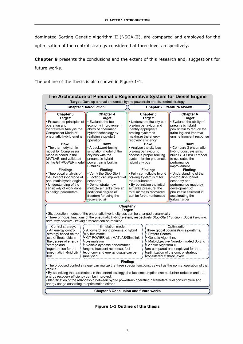
Figure 1-1 Outline of the thesis 3
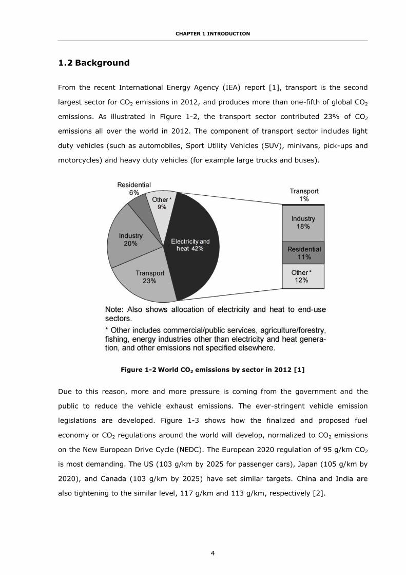
Figure 1-2 World CO2 emissions by sector in 2012 [1] 4
Figure 1-3 Comparison of finalized and proposed fuel economy or CO2 regulations around
the world, normalized to CO2 emissions on the NEDC [2] 5
Figure 1-4 Ragone chart - Energy vs. Power for various energy storage systems 6
Figure 1-5 Conceptual illustration of the hybrid powertrain 8
Figure 1-6 Series HEV configuration 10
Figure 1-7 Parallel HEV configuration 10
Figure 1-8 Combined (series-parallel) HEV configuration 10
Figure 1-9 Complex HEV configuration 11
Figure 1-10 Typical series HHV configuration 12
Figure 1-11 Typical pneumatic hybrid powertrain structure 13
Figure 2-1 Schematic diagram of Schechter’s proposed system [15] 22
Figure 2-2 Schematic diagram of 1st Brunel pneumatic hybrid engine [37] 23
Figure 2-3 Schematic diagram of Brunel 2nd pneumatic hybrid engine [36] 24
Figure 2-4 Schematic diagram of the air hybrid engine with an air starter [35] 25
Figure 2-5 Schematic diagram of Guzzella’s hybrid pneumatic engine [40] 26
Figure 2-6 Pneumatic hybrid concept using two tanks [21] 27
Figure 2-7 Schematic diagram of Higelin’s hybrid pneumatic engine [14] 29
xi
Figure 2-8 Schematic diagram of Tai’s hybrid pneumatic engine [17] 30
Figure 2-9 Schematic diagram of Kang’s air-power-assist engine [24] 31
Figure 2-10 MD11 air hybrid configuration [65] 32
Figure 3-1 Schematic diagram of the pneumatic hybrid engine 36
Figure 3-2 Tank temperatures for 1500 r/min engine speed [34] 38
Figure 3-3 Experimental and predicted air tank temperature at 1500 r/min engine speed
for 700 engine cycles [4] 39
Figure 3-4 Theoretical valve timing diagram of the normal operation mode and CM 40
Figure 3-5 Ideal p-V diagram during the CM 42
Figure 3-6 Schematic diagram of the start of the Compression Stroke in CM 43
Figure 3-7 Schematic diagram of the CREB intake valve opens during the Compression
Stroke in CM 44
Figure 3-8 Schematic diagram of the end of the Compression Stroke in CM 45
Figure 3-9 Schematic diagram of the start of the Intake Stroke in CM 46
Figure 3-10 Modified p-V diagram during the CM 47
Figure 3-11 Schematic diagram of the control volume 48
Figure 3-12 p-V diagram comparison 52
Figure 3-13 Pressure diagram in the CM 54
Figure 3-14 p-V diagram at 1500 rpm engine speed 55
Figure 3-15 Brake torque for various air tank pressure and engine speed 55
Figure 3-16 Brake torque for different intake timings 56
Figure 3-17 Brake torque for various engine speeds and the actual compression ratio 57

xii
Figure 4-1 Schematic diagram of the pneumatic hybrid engine with one air tank 60
Figure 4-2 Two air tanks pneumatic hybrid system structure 63
Figure 4-3 Pneumatic hybrid vehicle simulation model 64
Figure 4-4 Braunschweig driving cycle time–speed diagram 67
Figure 4-5 MLTB driving cycle time–speed diagram 67
Figure 4-6 One air tank simulation model control block 70
Figure 4-7 The state diagram of control strategy for one air tank model 71
Figure 4-8 One air tank model Stateflow diagram in Simulink 72
Figure 4-9 Two air tanks model control block 74
Figure 4-10 The state diagram of control strategy for two air tanks model 75
Figure 4-11 Two air tanks model Stateflow diagram in Simulink 76
Figure 4-12 Engine speeds during Braunschweig driving cycle 77
Figure 4-13 Air tank pressure of one air tank model during Braunschweig driving
cycle 78
Figure 4-14 Air tanks pressure of two air tanks model during Braunschweig driving
cycle 78
Figure 4-15 Air mass charged and discharged of one air tank model 79
Figure 4-16 Total air mass recovered of one and two air tanks model 79
Figure 4-17 Fuel consumption throughout the Braunschweig driving cycle 80
Figure 4-18 Engine speeds during MLTB driving cycle 81
Figure 4-19 Air tank pressure of one air tank model during MTLB driving cycle 82
Figure 4-20 Air tanks pressure of two air tanks model throughout MLTB driving cycle 83

xiii
Figure 4-21 Fuel consumption throughout the MLTB driving cycle 84
Figure 5-1 Traction and braking power dissipation in Braunschweig driving cycle 89
Figure 5-2 Deceleration distribution during Braunschweig driving cycle 89
Figure 5-3 Deceleration distribution during MLTB driving cycle 90
Figure 5-4 Schematic diagram of the engine with pneumatic regenerative system 91
Figure 5-5 Control strategy for the parallel hybrid braking system 92
Figure 5-6 IMEP in a Type 1 compression-braking cycle [63] 96
Figure 5-7 Control strategy for the fully controllable hybrid braking system 98
Figure 5-8 Pneumatic hybrid braking optimisation simulation model 101
Figure 5-9 Trace of objective function value over iterations of the optimisation 102
Figure 5-10 The increment of pressure during the driving based on different initial air
tank pressure 102
Figure 5-11 Two air tanks pneumatic hybrid engine structure 104
Figure 5-12 Air tanks pressure of two air tanks model during Braunschweig driving
cycle 105
Figure 5-13 Air tanks pressure of two air tanks model during MLTB driving cycle 105
Figure 5-14 Air mass recovery during the Braunschweig driving cycle 106
Figure 6-1 Typical map of aerodynamic type turbocharger compressor 112
Figure 6-2 Classification of various method of reducing turbo-lag 114
Figure 6-3 Main mechanism of improving turbocharger transient response 115
Figure 6-4 System diagram of PBS integration and PBS key component [85] 117

xiv
Figure 6-5 Torque curve of an 8-l-diesel engine with EGR and 2-stage turbocharging
with/without PBS [85] 117
Figure 6-6 System diagram of BREES [87] 118
Figure 6-7 The effect of compressed air injection on brake torque and turbocharger
speed [87] 119
Figure 6-8 Schematic diagram of diesel engine with EAT 120
Figure 6-9 Alternative combined supercharging configuration with electrically driven
compressor [86] 120
Figure 6-10 The diagram of engine structure can realize the Intake Side Boost 123
Figure 6-11 System diagram of System I 124
Figure 6-12 Effect of air-injection on transient response after a load step of 60%
full-load [86] 125
Figure 6-13 Different engine transient responses on the turbocharger compressor
map [88] 126
Figure 6-14 System diagram of System IP 127
Figure 6-15 System diagram of System E 128
Figure 6-16 GT-POWER model of the basic engine 130
Figure 6-17 GT-POWER model of the engine with System I 131
Figure 6-18 System diagram of System I control-unit 133
Figure 6-19 Flow chart of the System I control strategy 133
Figure 6-20 GT-POWER model of the engine with System IP 134
Figure 6-21 System diagram of System IP control-unit 136
Figure 6-22 Flow chart of the System IP control strategy 137
xv
Figure 6-23 GT-POWER model of the engine with System E 138
Figure 6-24 System diagram of System E control-unit 139
Figure 6-25 Flow chart of the System E control strategy 140
Figure 6-26 Brake torque response for each pneumatic hybrid boost system 141
Figure 6-27 Intake manifold pressure for each pneumatic hybrid boost system 142
Figure 6-28 Air tank pressure for each pneumatic hybrid boost system 143
Figure 6-29 TC-Shaft speed for each pneumatic hybrid boost system 144
Figure 6-30 Turbocharger operation points on compressor efficiency map for each
pneumatic hybrid boost system 145
Figure 6-31 The basic vehicle simulation model 147
Figure 6-32 The vehicle with System I simulation model 147
Figure 6-33 The vehicle with System IP simulation model 148
Figure 6-34 Vehicle speed during the acceleration 148
Figure 6-35 Engine brake torque response during the acceleration 149
Figure 6-36 Air tank pressure drop during the acceleration 150
Figure 7-1 Classification of hybrid vehicle control strategies 154
Figure 7-2 Schematic diagram of the control strategy for pneumatic hybrid city bus 160
Figure 7-3 Schematic diagram of the control strategy optimisation 161
Figure 7-4 Operation modes for the pneumatic hybrid city bus 163
Figure 7-5 State diagram of control strategy for the pneumatic hybrid city bus 166
Figure 7-6 Stateflow diagram of control strategy for the pneumatic hybrid city bus 167
Figure 7-7 The pneumatic hybrid city bus GT-POWER part simulation model 169
xvi
Figure 7-8 The pneumatic hybrid city bus MATLAB/Simulink part simulation model 170
Figure 7-9 Forward facing hybrid vehicle model 171
Figure 7-10 Engine and pneumatic regenerative system model in GT-POWER 172
Figure 7-11 Forces acting on the city bus 173
Figure 7-12 Vehicle subsystem model in GT-POWER 175
Figure 7-13 Input and output of the driver model 177
Figure 7-14 Air tanks energy recovery model in MATLAB/Simulink 177
Figure 7-15 Braunschweig-H time–speed diagram 179
Figure 7-16 Braunschweig driving cycle time–speed diagram 180
Figure 7-17 Acceleration behaviours of the Braunschweig driving cycle 181
Figure 7-18 Brake behaviours of the Braunschweig driving cycle 182
Figure 7-19 Simulation results of the control strategy of the pneumatic hybrid city bus
comparing with the normal city bus 183
Figure 7-20 Brake torque for the first 10 s 185
Figure 7-21 Brake specific fuel consumption for the first 10 s 185
Figure 7-22 Average fuel consumption during the Braunschweig-H 186
Figure 7-23 Total energy dissipated during the braking 187
Figure 7-24 Air tanks pressure during the Braunschweig-H 187
Figure 7-25 Trace of objective function value over iterations of PS optimisation 193
Figure 7-26 Flow chart of optimisation simulation model based on GA 197
Figure 7-27 Trac of objective minimization over generations 199
Figure 7-28 Optimal Pareto front for the multi-objective optimisation using NSGA-II 207

xvii
LIST OF TABLES
Table 1-1 The operation conditions of hybrid powertrain 8
Table 1-2 Key features of HEV 11
Table 1-3 The versions of the software used in the research 18
Table 2-1 Summary table of fuel consumption result 33
Table 3-1 Main technical parameters of the engine and pneumatic hybrid system 37
Table 3-2 Parameters setting of the simulation 52
Table 3-3 Theoretical model engine brake torque (Nm) map 53
Table 3-4 GT-POWER model engine brake torque (Nm) map 53
Table 4-1 Air starter performance information [68] 61
Table 4-2 SS175 number of starts per tank [68] 62
Table 4-3 City bus data [34] 66
Table 4-4 Basic parameters of the MLTB driving cycle and Braunschweig driving cycle 68
Table 4-5 Summary table of fuel consumption improvements 85
Table 5-1 Basic parameters of the Braunschweig driving cycle 87
Table 5-2 City bus data 88
Table 5-3 Design variable for initial air tank pressure optimisation 100
Table 5-4 Pattern Search optimisation result 101
Table 5-5 Two air tanks pneumatic hybrid city bus parameter data 103

xviii
Table 5-6 Comparison of air mass recovered during Braunschweig driving cycle between
the new control strategy and the previous one 107
Table 6-1 Main technical parameters of YC6A series engines [89] 130
Table 6-2 Dimensions and characteristics of System I 132
Table 6-3 Dimensions and characteristics of System IP 135
Table 6-4 Dimensions and characteristics of System E 138
Table 6-5 Time to reach peak torque output of the four engine configurations 141
Table 6-6 Air tank pressure drops of the pneumatic hybrid boost systems 143
Table 6-7 City bus parameters 146
Table 6-8 Time to reach the speed of 48km/h 149
Table 7-1 Parameters of the logic threshold control strategy for the pneumatic hybrid
city bus 162
Table 7-2 Conditions and output signals of the control strategy 168
Table 7-3 Main technical parameters of the engine and pneumatic regenerative
system 172
Table 7-4 Summary the function of the parts in the vehicle subsystem 176
Table 7-5 Stop-start events and acceleration-deceleration events 181
Table 7-6 Basic parameters of the Braunschweig driving cycle and Braunschweig-H 182
Table 7-7 RMSE of normal city bus and pneumatic hybrid city bus to the target driving
cycle speed 184
Table 7-8 Summary table of the optimisation problems and methods 189
Table 7-9 Design variables for PS optimisation 191
Table 7-10 Summary table for PS optimisation 192

xix
Table 7-11 PS optimisation result 193
Table 7-12 The terminology of GA 196
Table 7-13 Design variables for genetic algorithm optimisation 198
Table 7-14 Summary table for GA optimisation 198
Table 7-15 GA optimisation result 199
Table 7-16 The gear changing strategy during the braking after optimisation 199
Table 7-17 Design variables for multi-objective optimisation 203
Table 7-19 Summary table for NSGA-II optimisation 204
Table 7-20 The options of two multi-objective optimisations 205
Table 7-21 Multi-objective optimisation 1 result 205
Table 7-22 Multi-objective optimisation 2 result 206
Table 7-23 The gear changing strategy during the acceleration after optimisation 208
Table 7-24 Parameters in the pneumatic hybrid city bus control strategy after
optimisation 209
Table 7-25 Fuel consumption before and after optimisations 209

xx
NOMENCLATURE
Latin Letters
A [m2, J] Open area of the valve, Frontal area of the vehicle, Availability
a [m] Distance from gravity centre to front wheel centre
b [m] Distance from the gravity centre to front wheel centre
C [-] Constant, Discharge coefficient, Drag coefficient, Specific heat
c [-] Constant
D [s] Duration of the intake valve second opening in crank angle
E [J] Energy
F [N] Braking force, Friction
f [-] Rolling resistance coefficient
G [-, m/s2] Rotating inertia, Gravity of the vehicle
g [m/s2] Gravitational acceleration
h [m] Height
i [-] Number of the cylinders
𝑗 [m/s2] Deceleration rate of the vehicle
k [-] Ratio of specific heats
L [m] Wheel base
M [kg] Vehicle mass
m [g] Air mass
N [rpm, -] Engine speed, Number
n [-] Polytropic index
P [kW] Power
p [bar] Pressure

xxi
R [-] Ideal gas constant, Geometric compression ratio
r [-] Compression ratio
T [k, Nm] Temperature, Torque
t [s] Time
v [m/s] Speed
V [l] Volume
W [J] Work, Load
Greek Symbols
α [-] Constant
δ [-] Rotational inertia factor
η [-] Efficiency
ρ [kg/m3] Density
τ [Nm] Torque
μ [-] Friction coefficient, Adhesion coefficient, Control variables
ω [rad/s] Angular velocity
Subscripts and Superscripts
0 Intake manifold, Initial
a Air
aux Auxiliary Chamber
c Cylinder clearance, Compressor
D Aerodynamic
d Driving
dis Discharge cases
e Measured

xxii
f Front, Final
final Final point
g Gravity centre
in Upstream
m Motor
max Maximum
min Minimum
out Downstream
R Crank revolutions for each power stroke per cylinder
r Rear, Tire, Rolling
rech Recharge cases
s Cylinder swept
T Turbine
t Air tank, Traction
TC Turbocharger
w Aerodynamic friction
Abbreviations
AC Air Compression
AM Air Motor
ATV Air Tank Valve
BDC Bottom Dead Centre
BREES BRaking Exhaust Energy Storage
CA Crank Angle
CB Compression Braking
CM Compressor Mode
CPS Cam Profile Switching

xxiii
CREB Compression Release Engine Braking
CV Check Valve
DP Dynamic Programming
EAT Electric Assist Technology
ECE Economic Commission of Europe
ECMS Equivalent Consumption Minimization Strategy
ECV Energy Control Valve
EGR Exhaust Gas Recirculation
EHV Electro-Hydraulic Valvetrain
EM Expander Mode
EPSRC Engineering and Physical Sciences Research Council
ESB Exhaust Side Boost
EV Electric Vehicle
GA Genetic Algorithm
GPS Generalized Pattern Search
HEV Hybrid Electric Vehicles
HHV Hydraulic Hybrid Vehicle
HIL Hardware-In-the-Loop
ICE Internal Combustion Engine
IEA International Energy Agency
IM Improvement Method
IMEP Indicated Mean Effective Pressure
IMV Intake Manifold Valve
IPV Intake Port Valves
ISB Intake Side Boost
IVSC Intake Valve Second Close
MDI Motor Development International

xxiv
MLTB Millbrook London Transport Bus
MOGA Multi-Objectives Genetic Algorithm
MOO Multi-objective optimisation
MVEG Motor Vehicle Emissions Group
NA Naturally Aspirated
NEDC New European Drive Cycle
NSGA Nondominated Sorting Genetic Algorithm
NSGA-II Nondominated Sorting Genetic Algorithm II
PBS Pneumatic Boost System
PS Pattern Search
p-V Pressure-Volume
QSS-TB Quasi Steady State Toolbox
RegenEBD Regenerative Engine Braking Device
RMSE Root Mean Square Error
SAE Society of Automotive Engineers
SFC Specific Fuel Consumption
SIL Software-In-the-Loop
SOC State of Charge
SOGA Single Objective Genetic Algorithm
SPEA Strength Pareto Evolutionary Algorithm
SUV Sport Utility Vehicles
TDC Top Dead Centre
TV Throttle Valve
VGT Variable Geometry Turbine
YUCHAI Guangxi Yuchai Machinery Company Limited

CHAPTER 1 INTRODUCTION
1
CHAPTER 1
INTRODUCTION
1.1 Introduction and Outline of the Thesis
This research is based on the project, A Cost-Effective Regenerative Air Hybrid
Powertrain for Low Carbon Buses and Delivery Vehicles, which is supported by the UK
Engineering and Physical Sciences Research Council (EPSRC) under grant reference
EP/I00601X/1. It is carried out as part of a joint project between Loughborough
University and Brunel University London. The pneumatic hybrid system hardware design
and engine experimental research have been conducted at Brunel University London,
while the pneumatic hybrid system and vehicle modelling, simulation research and
control methodology development have been studied at Loughborough University.
Guangxi Yuchai Machinery Company Limited (YUCHAI) provides a six-cylinder diesel
engine to Brunel University London, and modifies it to realize the proposed pneumatic
hybrid system operations.
Chapter 1 gives an overview of the structure of the thesis. Then the research
background and motivation are analysed. Research aims and objectives are also
summarized. Finally, the methodology and software using in the research are introduced.
Chapter 2 is a review of relevant literatures to identify specific research gaps and
narrow down the focus. It firstly summaries the compressed air vehicle and air engine
history. Then the state-of-the-art of pneumatic hybrid technology research is presented.
The literature review supports and defines the scope of the chosen research topics and
summarizes those topics that lie outside the scope.
Chapter 3 presents the principle of operation and confirms the potential of the
pneumatic hybrid system to both generate a supply of compressed air and to manage the
contribution of the engine to vehicle braking. The pneumatic hybrid engine Compressor
Mode (CM) is considered from a theoretical perspective based on an air cycle analysis
CHAPTER 1 INTRODUCTION
2
and validated. Finally an understanding of the sensitivity of work done (braking torque
created during the CM) to design parameters is given.
Chapter 4 presents an evaluation of the fuel economy improvement ability of pneumatic
hybrid technology for the city bus application by realizing the Stop-Start Function
through different bus driving cycles. Also, an investigation is made into how multiple air
tanks give an additional degree of freedom for management of recovered air. A
backward-facing simulation model of the city bus with the pneumatic hybrid powertrain
has been applied to investigate the improvement of fuel economy by using one and two
air tanks in different driving cycle.
Chapter 5 presents an analysis of vehicle braking behaviour through different bus
driving cycles and compares two configurations of the hybrid braking system, the parallel
hybrid brake system and the fully controllable hybrid brake system. The comparison
shows the fully controllable hybrid braking system has a distinct advantage and is chosen
to realize the regenerative braking function. A braking simulation model has been built in
to support an investigation of an optimum air tank pressure and configuration for energy
recovery.
Chapter 6 presents an analysis of the reasons for engine turbo-lag and the methods
developed for reducing the turbo-lag and improving transient response first. Then, a
number of architectures for managing a rapid energy transfer into the powertrain to
assist acceleration of the turbocharger have been proposed and investigated from two
aspects, engine brake torque response and vehicle acceleration, by using the 1-D engine
simulation.
Chapter 7 presents the design of an energy control strategy based on the use of
thresholds in the degree of energy storage and regeneration (a “logic threshold”
methodology) for the pneumatic hybrid city bus. A forward facing pneumatic hybrid city
bus simulation model has been developed in GT-POWER with MATLAB/Simulink co-
simulation. To obtain the maximum overall fuel economy, the amount of air and energy
recovered during the braking and minimum loss of availability during acceleration, a
number of variables in the control strategy must be optimized. Three global optimisation
algorithms, Pattern Search (PS), Genetic Algorithm (GA) and multi-objective Non-
CHAPTER 1 INTRODUCTION
3
dominated Sorting Genetic Algorithm II (NSGA-II), are compared and employed for the
optimisation of the control strategy considered at three levels respectively.
Chapter 8 presents the conclusions and the extent of this research and, suggestions for
future works.
The outline of the thesis is also shown in Figure 1-1.
Figure 1-1 Outline of the thesis
CHAPTER 1 INTRODUCTION
4
1.2 Background
From the recent International Energy Agency (IEA) report [1], transport is the second
largest sector for CO2 emissions in 2012, and produces more than one-fifth of global CO2
emissions. As illustrated in Figure 1-2, the transport sector contributed 23% of CO2
emissions all over the world in 2012. The component of transport sector includes light
duty vehicles (such as automobiles, Sport Utility Vehicles (SUV), minivans, pick-ups and
motorcycles) and heavy duty vehicles (for example large trucks and buses).
Figure 1-2 World CO2 emissions by sector in 2012 [1]
Due to this reason, more and more pressure is coming from the government and the
public to reduce the vehicle exhaust emissions. The ever-stringent vehicle emission
legislations are developed. Figure 1-3 shows how the finalized and proposed fuel
economy or CO2 regulations around the world will develop, normalized to CO2 emissions
on the New European Drive Cycle (NEDC). The European 2020 regulation of 95 g/km CO2
is most demanding. The US (103 g/km by 2025 for passenger cars), Japan (105 g/km by
2020), and Canada (103 g/km by 2025) have set similar targets. China and India are
also tightening to the similar level, 117 g/km and 113 g/km, respectively [2].

CHAPTER 1 INTRODUCTION
5
Figure 1-3 Comparison of finalized and proposed fuel economy or CO2 regulations around
the world, normalized to CO2 emissions on the NEDC [2]
Now, the automotive industry is facing the biggest revolution in its history. Historically,
engine technologies were largely influenced by and developed for meeting criteria
emissions regulations [3]. Due to hybrid powertrain and pure battery electric powertrain
technologies development, the traditional engines start to be replaced by the hybrid
powertrain or even entirely by the pure battery electric powertrain. But for the short to
medium term, hybrid powertrain with regenerative recovery is recognised as one of the
most effective means to reduce CO2 emissions for the automotive industry [4].
1.3 Hybrid Vehicle
A hybrid vehicle is defined by Society of Automotive Engineers (SAE) as: A vehicle with
two or more energy storage systems both of which must provide propulsion power –
either together or independently [5]. It aim to have the advantages of both IC engine
and other kind powertrain systems [6]. The “energy storage systems” in hybrid vehicle
could be a gasoline or diesel engine, electric motor/battery pack, or other source of
motive power. The goal of the hybrid vehicle is to provide the equivalent performance
range and safety as a conventional vehicle while reducing fuel consumption and harmful
emissions by better managing the two or more energy source. The reason for using more
CHAPTER 1 INTRODUCTION
6
than one power sources is because of the disadvantages of conventional vehicles with
Internal Combustion (IC) engines like the low fuel economy and high environmental
pollution. These disadvantages cause by the mismatch of engine fuel efficiency
characteristic with the real operation requirement, dissipation of vehicle kinetic energy
during braking and low efficiency of hydraulic transmission in the current vehicle in stop-
start function [6]. Compare with petroleum fuels, other power resources like electric
powertrain, hydraulic powertrain and pneumatic powertrain have some advantages such
as high-energy efficiency and lower environmental pollution. But these powertrains also
have some disadvantages such as low energy density and high cost.
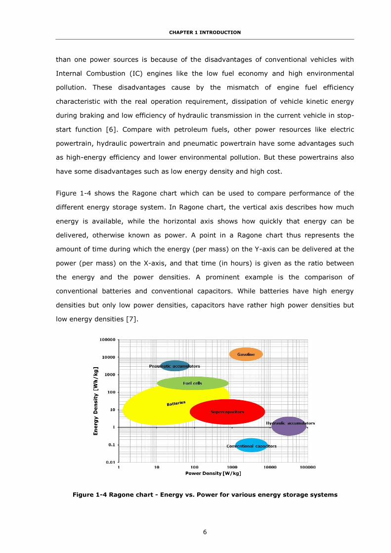
Figure 1-4 shows the Ragone chart which can be used to compare performance of the
different energy storage system. In Ragone chart, the vertical axis describes how much
energy is available, while the horizontal axis shows how quickly that energy can be
delivered, otherwise known as power. A point in a Ragone chart thus represents the
amount of time during which the energy (per mass) on the Y-axis can be delivered at the
power (per mass) on the X-axis, and that time (in hours) is given as the ratio between
the energy and the power densities. A prominent example is the comparison of
conventional batteries and conventional capacitors. While batteries have high energy
densities but only low power densities, capacitors have rather high power densities but
low energy densities [7].
Figure 1-4 Ragone chart - Energy vs. Power for various energy storage systems

CHAPTER 1 INTRODUCTION
7
From Figure 1-4, it can be seen that the supercapacitors have an unusually high energy
density. They have advantages such as high energy storage compared to conventional
capacitor technologies and fast charge and discharge ability. As can be seen in Figure 1-4,
the supercapacitors reside in between batteries and conventional capacitors. They are
typically used in applications where batteries have a short fall when it comes to high
power and life, and conventional capacitors cannot be used because of a lack of energy,
and offer a high power density along with adequate energy density for most short term
high power applications.
From Figure 1-4, it also can be seen that hydraulic accumulators are one kind of short-
term storage systems which have the ability to accept high rates and high frequencies of
charging/discharging. The devices are characterized by a lower energy density and
higher power density than electrochemical batteries. It can supply very high density of
power. The hydraulic hybrid system can easily capture the vehicle braking energy.
Because of the high efficiency of the system components such as the accumulator and
the pump/motor, the operational efficiencies can exceed 70% which is far better than
any other form of hybridization such as batteries system [8, 9]. However, hydraulic
hybrid technology has several limitations such as its relatively low energy density and
limited storage of energy which restricts the time of continuous operation.
The pneumatic accumulators pressurises air as the energy storage medium. Compressed
air has relatively low energy density. Air at 300 bar (30 MPa) contains about 50 Wh of
energy per liter [9]. For comparison, a lead–acid battery contains 60-75 Wh/l energy
density; and a lithium-ion battery contains about 250-620 Wh/l energy density. Although
the pneumatic accumulators cannot be used as an energy source to drive the vehicle
alone, it can be a supplementary to the IC engine in the HEV.
The braking energy is the only energy the vehicle can earn without any energy cost. But
the conventional IC engine cannot get this energy and reuse it. Normally, a hybrid
vehicle has a powertrain can recover this energy. For the purpose of getting the
maximum braking energy, a hybrid powertrain usually has a powertrain that allow energy
to flow backward from the wheel to the energy source and another one can flow either
forward or backward. Figure 1-5 shows the concept of the hybrid powertrain and the
possible different power flow routes.

CHAPTER 1 INTRODUCTION
8
Figure 1-5 Conceptual illustration of the hybrid powertrain
From Table 1-1, there are 9 operation conditions of the hybrid powertrain to meet the
load requirement:
Table 1-1 The operation conditions of hybrid powertrain
Condition Powertrain 1 Powertrain 2
1 Deliver power to load -
2 - Deliver power to load
3 Deliver power to load Deliver power to load
4 - Obtain power from load
5 Deliver power to Powertrain 2 Obtain power from Powertrain 1
6 Deliver power to Powertrain 2 Obtain power from Powertrain 1
and load
7 Deliver power to load and Powertrain 2 Obtain power from Powertrain 1
8 Deliver power to Powertrain 2 Deliver power to load
9 Deliver its power to load Obtain power from load

CHAPTER 1 INTRODUCTION
9
Usually, more than two power sources in a hybrid vehicle will make the propulsion
system very complicated. This kind of hybrid vehicle will not be discussed in this research.
1.3.1 Hybrid Electric Vehicle
Normally, the term hybrid vehicle most often refers to the Hybrid Electric Vehicle (HEV),
which consists of an IC engine and one or more electric motors. The reason for using
more than one electric motor is that the second one works as an electricity generator to
charge the battery. The energy storage for HEV is usually a battery or in some cases, a
supercapacitor.
Before 2000, the HEVs usually classified two basic types: series and parallel. In 2000,
some newly introduced HEVs cannot be classified into these two types. Hence, the
combined series-parallel HEV and complex HEV added into the hybrid vehicle family [6].
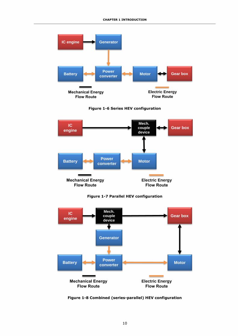
The HEV is classified into four types:
(i) Series HEV: the electric motor propels the vehicle alone, the electricity can be
obtained from either battery or an electricity generator driven by IC engine.
(ii) Parallel HEV: the IC engine and the electric motor can propel the vehicle
individually or simultaneously.
(iii) Combined (series-parallel) HEV: this kind of hybrid vehicle has a power-split
device allowing for power flow routes from the engine to the wheels that can be
either mechanical or electrical.
(iv) Complex HEV: similar with the combined hybrid, but the electric coupling
function is moved from the power converter to the battery and one more power
converter is added between the motor/generator and the battery [6].
The configurations of four kinds of HEVs are shown in Figure 1-6 to Figure 1-9. The key
features of four types HEV are compared in the Table 1-2.
CHAPTER 1 INTRODUCTION
10
Figure 1-6 Series HEV configuration
Figure 1-7 Parallel HEV configuration
Figure 1-8 Combined (series-parallel) HEV configuration
Motor
IC engine Generator
Battery
Electric Energy
Power
converter Gear box
Motor
IC
engine
Mech. couple
device
Battery
Electric Energy
Power
converter
Gear box
Motor
IC
engine
Mech. couple
device
Battery
Electric Energy
Power
converter
Gear box
Generator

CHAPTER 1 INTRODUCTION
11
Figure 1-9 Complex HEV configuration
Table 1-2 Key features of HEV
Series HEV Parallel HEV
Combined
(series-parallel) HEV
Complex HEV
Key
feature
Two electric powers
are added together in
the power converter, an electrical power
couple device
Two mechanical
powers are added
together in a mechanical power
couple device
Using both
mechanical and
electrical power couple device
together
Similar with
combined HEV, but
using battery to be an electrical power
couple device
The most researched and developed hybrid vehicles are electric based. But the
applications of the electric hybrid powertrain to buses, trucks and delivery vehicles are
limited by the huge additional cost of numbers of batteries and the cost to combined
electric and mechanical powertrain and transmission systems together. From
Ranganathan’s report, the average price of a 12 m hybrid bus typically ranges from
$450,000 - $550,000 when compared to $280,000 - $300,000 for a conventional diesel
bus [10]. The price variation in hybrids is due to the order volumes and individual
specifications. In UK, there are currently a few of electric hybrid buses operating in some
cities. Such electric hybrid buses can cost additional £100,000 to rebuild or manufacture,
they need heavily finical support and will not be fit for commercially viable large volume
production in this stage [11].
Motor
IC
engine
Mech. couple
device
Battery
Electric Energy
Power converte
r
Gear box
Motor/Ge
nerator
Power converte
r

CHAPTER 1 INTRODUCTION
12
1.3.2 Hydraulic Hybrid Vehicle
The Hydraulic Hybrid Vehicle (HHV) is based on the hydraulic hybrid powertrain which
includes an IC engine and a hydraulic pump/motor [12]. The energy stores in the
hydraulic accumulator. The HHVs also can divide into series and parallel two types.
Figure 1-10 is a typical series HHV configuration.
Figure 1-10 Typical series HHV configuration
All types of hydraulic hybrid powertrain include a high-pressure accumulator and a low-
pressure reservoir. The accumulator contains the hydraulic fluid and a gas such as
nitrogen (N2) or methane (CH4), separated by a membrane. When the hydraulic fluid
flows in, the gas is compressed. During the discharge phase, the fluid flows out through
the motor and then into reservoir [6].
Due to the characteristic of the hydraulic fluid and hydraulic accumulator, the hydraulic
hybrid powertrain has the ability to accept both high frequencies and high rate of
charging/discharging operations, such as the NYC COMP cycle, which has an average of
4.96 stops per km and an average kinetic intensity of 2.67 per km [13]. This feature is fit
for recovering the vehicle’s kinetic energy during braking. That means the hydraulic
hybrid powertrain is the ideal choice for the buses and delivery vehicles in cities and
urban areas where the traffic conditions involve a lot of stop-start operations. Compare
with the electric hybrid powertrain, the hydraulic hybrid powertrain for trucks and buses
can be less expensive by using the hydraulic accumulator as an energy storage device
instead of the high price amount of batteries.
Hydraulic motor/
pump
IC
Engine
Hydraulic
pump
Hydraulic
accumulator
Hydraulic Energy
Power
converter Gear box

CHAPTER 1 INTRODUCTION
13
Similarly with the HEVs, the hydraulic hybrid vehicles will be added a completely separate
and additional unit, the cost and weight would be expected as high as the equivalent
HEVs.
1.3.3 Pneumatic Hybrid Vehicle
The pneumatic hybrid vehicle is based on pneumatic hybrid powertrain which typically
using the fully variable actuation valve to change the conventional IC engine to a
pneumatic pump and a pneumatic motor [14-24]. A typical pneumatic hybrid powertrain
structure is shown in Figure 1-11.
Figure 1-11 Typical pneumatic hybrid powertrain structure
Because of the existing of the fully variable actuation valve, during the compression
stroke, the IC engine can compress the air into high pressure air tank, and at the intake
stroke, the high pressure air stored in the air tank can come into the cylinder and propel
the piston. In the pneumatic hybrid powertrain, the energy storage device is the air tank.
Because of the energy density of air, the pneumatic hybrid powertrain similar with the
hydraulic hybrid powertrain is fit for accepting both high frequencies and high rate of
charging/discharging operations. This feature can significantly improve the fuel economy
by implementing regenerative energy recovery operation, particularly for buses and
delivery vehicles in cities and urban areas where the working conditions include a lot of
stop-start operations [11]. Because of in such conditions, a large amount of fuel is
needed to accelerate the vehicle, and much of this is converted to heat in brake friction
during deceleration. Capturing, storing and reusing this braking energy can therefore
improve fuel efficiency, and this can be achieved by using the momentum of the vehicle

CHAPTER 1 INTRODUCTION
14
during coasting and deceleration to charge the energy storage device and later reuse the
energy to save the fuel consumption.
Moreover, a pneumatic hybrid powertrain ideally complements a down-size and
supercharged engine [16, 25]. In fact, turbocharged engines usually have a turbo-lag
because the relatively slow acceleration of the compressor-turbine during load steps.
Although by choosing small turbines, which minimize the delays but will cause a rather
lower efficiency [16]. In the pneumatic hybrid powertrains, the air available in the air
tank is provided to the cylinder by a fully variable charge valve during in the heavy
transients, the torque can be raised from idling to full-load from one engine cycle to the
next or in the shortest time possible. Also, this will give more freedom to design the
turbines for an optimal economy. Moreover, the combustion with the large amount of
fresh air and fuel accelerates the turbocharger much faster, resulting in a fast pressure
rise in the intake manifold. Therefore, the additional air from the pressure tank is needed
only for a very short time such that relatively small air tanks can be used [16].
Unlike the electric and hydraulic hybrid vehicles, pneumatic hybrid vehicles can be
implemented without adding an additional propulsion system to the vehicle when it has
already applied an IC engine. In this case, the engine transmitting power through the
pistons and the crankshaft of the engine by working as a compressor during
braking/deceleration or an air motor at starting/acceleration. The vehicles can use the
existing braking or propelling drivetrain. For buses and delivery vehicles, air energy will
be stored in a moderate pressure compressed air storage tank already available on such
vehicles. Compare with HEVs and HHVs, the pneumatic hybrid vehicles do not need add
the large weight and complexity modifications to the vehicle. In addition, the stored high
pressure air is available readily in demand for other uses to improve drivability and
reduce emissions, such as briefly boosting the engine to eliminate turbo-lag in a turbo-
charged engine resulting in better response and removal of the black smoke typically
seen from accelerating diesel vehicles. For buses and commercial vehicles, compressed
air is required for air assisted braking system and the operation of pneumatic equipment
(e.g. door opening and closing) and is currently produced by an engine driven
compressor. Pneumatic hybrid powertrain technology will enable further and readily
achievable fuel savings to be realized by providing the service compressed air from the
regenerative engine braking in place of the engine driven compressor. Finally, the
CHAPTER 1 INTRODUCTION
15
compressed air produced can also be used briefly in combination with the Exhaust Gas
Recirculation (EGR) in a diesel engine to improve the dynamic trade-off between NOx and
smoke emissions. These are exciting synergies enhancing many attributes of the engine
at minimum cost and are immediately available, not possible with the other hybrid
energy types and unique only with the pneumatic hybrid because of the readily available
air supply. Therefore, the exploitation of such synergies will result in a pneumatic hybrid
powertrain system with significant and concurrent improvements in fuel consumption,
emission, and performance.
1.4 Research Aims and Objectives
For vehicles whose duty cycle is dominated by start-stop operations, fuel consumption
may be significantly improved by better management of the start-stop process.
Pneumatic hybrid technology represents one technology pathway to realise this goal.
Vehicle kinetic energy is converted to pneumatic energy by compressing air into the air
tanks installed in the vehicle. The compressed air is reused (i) to power an air starter to
realize the stop-start operation, (ii) to supply energy to the air path in order to reduce
turbo-lag. However, there has been no in-depth study yet that how to implement the
pneumatic hybrid technology on the city bus and realize these two functions.
To close this gap, this research therefore aims to develop a novel pneumatic hybrid
powertrain for city bus applications and its control strategy with significant and
concurrent improvements in fuel economy and performance over the current IC engines.
The proposed pneumatic hybrid powertrain offers a clear and low-cost alternative to the
electric hybrid technology in improving fuel economy, and vehicle drivability.
The specific objectives are:
(i) To fully understand the principle of the operation of the pneumatic hybrid engine
and the quantification of the sensitivity of the work done to design parameters
during the Compressor Mode.
(ii) To evaluate the fuel economy improvement ability of pneumatic hybrid
technology for the city bus through different bus driving cycles.
(iii) To analyse engine braking characteristics during the vehicle’s deceleration and
braking process during different bus driving cycles and hence identify

CHAPTER 1 INTRODUCTION
16
appropriate braking system structure and its control strategy for maximum
energy recovery.
(iv) To study the benefits of extra boost on reducing turbo-lag, improved engine
performance, and reduce fuel consumption.
(v) To formulate a pneumatic hybrid city bus control strategy and the vehicle driving
cycle simulation programme and identify the relationship between respectively
the operating parameters, fuel consumption and energy usage according to
optimisation criteria.
1.5 Methodology and Software
Methodology
Approaches of both theoretical analysis and computer simulation are chosen for this
research. During the whole research period, computer simulation research will conduct
with the aim to investigate the feasibility of the pneumatic hybrid engine concept and
develop the control strategy for the pneumatic hybrid city bus. Then, the simulation
result is compared and verified with the experimental result from the engine experiment
had already been carried out in Brunel University London before.
Two main approaches, backward facing simulation and forward facing simulation, are
used in the research. Backward facing simulation takes the assumption that the vehicle
meets the target requirement, and calculates the component states. On the contrast,
forward facing simulation simulates the physical behaviours of each component with
control instruction, handles state changes, and generates vehicle performance as output.
Backward facing approach is beneficial in simplicity and computation cost, while the
forward-facing approach is advantageous in exploiting performance details.
Software
There are several modelling tools can be utilised in the process of modelling hybrid
configurations and its control strategies. They can be divided into two types from the
simulation direction. The first one is based on the backward facing simulation method
which normally developed in the MATLAB/Simulink environment. Another is based on the

CHAPTER 1 INTRODUCTION
17
forward facing simulation method which normally includes the detailed engine model to
realize the 1-D simulation.
MATLAB®, developed by The MathWorks, Inc., can be used for creating and developing
mathematical models for engineering applications and solutions, the Simulink toolbox
components include specific items for developing controls, signal processing and real-
time programming [26]. Simulink provides a graphical editor, customizable block libraries,
and solvers for modelling and simulating dynamic systems [27]. It is integrated with
MATLAB, enabling the user to incorporate MATLAB algorithms into models and export
simulation results to MATLAB for further analysis [27].
GT-SUITE®, a product of Gamma Technologies Inc., is a single software tool for
modelling and simulation of systems in automotive and transportation industry as well as
in other industries [28, 29]. GT-SUITE can be used to develop different applications such
as [28]:
Engine performance modelling - including combustion and turbocharging
Exhaust after treatment
Hybrid and electric vehicles - electric machines, fuel cells
Vehicle dynamics - drive cycles, drivelines
GT-POWER®, part of the GT-SUITE, is a code for engine simulations. At its core, the GT-
POWER solver is based on the 1-D solution of the fully unsteady, nonlinear Navier-Stokes
equations. It is applicable to different sizes and types of engines, contains models for
engine performance analysis, and allow the engineer to analyse a number of engine
configurations and performance characteristics, including [30]:
Torque and power curves, airflow, vol. efficiency, fuel consumption, emissions
Steady state or full transient analysis, under different driving scenarios
Turbocharged, supercharged, turbocompound, e-boost, pneumatic assist
GT-SUITE also offers a toolbox for modelling vehicles and drivelines and simulation of
vehicle dynamics. Vehicle models can address a range of vehicle engineering issues:
vehicle performance, fuel economy, emissions, and etc. It furthermore offers a set of
tools for the simulation of vehicles with HEV or Electric Vehicle (EV) drivelines.

CHAPTER 1 INTRODUCTION
18
The versions of the software using in the research are listed in Table 1-3.
Table 1-3 The versions of the software used in the research
Chapter 3 Chapter 4 Chapter 5 Chapter 6 Chapter 7
MATLAB/Simulink R2012a R2012a R2012a - R2014a
GT-SUITE V7.3.0 - - V7.3.0 V7.4.0
1.6 Contributions to Knowledge
The work reported in this thesis establishes a new understanding of the principles of
application of pneumatic hybrid methods to the braking and drivability of heavy duty
vehicles. In particular:
(i) The representation of the thermodynamic process during the Compressor Mode
and the quantification of the sensitivity of the work done to the design
parameters.
(ii) The evaluation of the fuel economy improvement ability of pneumatic hybrid
technology for the city bus through different bus driving cycles.
(iii) Demonstrate how the proposed pneumatic hybrid powertrain contributes to
vehicle braking and identify the design guideline to integrate the pneumatic
braking system to the vehicle friction braking system.
(iv) The understanding of the contribution to fuel economy and performance made
by the pneumatic assistance in accelerating the turbocharger.
(v) The identification and quantification of the relationship between respectively the
pneumatic hybrid powertrain operating parameters, fuel consumption and
energy usage according to optimisation criteria.

CHAPTER 2 LITERATURE REVIEW
19
CHAPTER 2
LITERATURE REVIEW
2.1 Introduction
In this chapter, the history of the use of compressed air in vehicles is briefly introduced,
considering that the concept of both pneumatic hybrid engine and air engine has evolved
alongside the development of compressed air vehicles. Then the air engine and
pneumatic hybrid engine development are summarized. After that, five most active
pneumatic hybrid technology research groups’ achievements are introduced in detail. The
five research groups at different universities are: Brunel University London [31-37], ETH
University [16, 38-42], Lund Institute of Technology [21, 43-46], University of Orléans
[14, 19, 47-52], and UCLA Research Group [17, 24].
2.2 Compressed Air Vehicle History
A compressed air vehicle is defined as a vehicle powered by an air engine, using
compressed air, which is stored in a tank [53]. Instead of mixing fuel with air and
burning it in the engine to drive pistons with hot expanding gases, compressed-air
vehicles use the expansion of compressed air to drive the pistons [53].
The compressed air had been used to power locomotives and trams since the 19th
century [53-56]. The first compressed air vehicle was devised by Bompas, who
developed a patent for a locomotive being taken out in England in 1828. The patent had
two storage tanks between the frames, with conventional cylinders and cranks [54]. In
1872 and 1873, Louis Mekarski took out patents for the Mekarski system which was the
fundamental design for the most successful tramcars later [56]. The Mekarski system
had a single stage engine and a special design. The air was warmed before entering the
engine from air tank to overcome the common problem that the air cools as it expands,
which lead to the formation of ice in the power cylinders [57]. For the following half a
century, the air-powered locomotive was a serious contender for the top spot in
transportation because of its obvious advantages: simplicity, safety, economy, and

CHAPTER 2 LITERATURE REVIEW
20
cleanliness [55]. Until the 1930s and 1940s the air locomotive had no serious
competition from electric or internal combustion engines in the mining industry because
the heat and spark made these competitors unsafe in closed-in and gassy places [55].
In 1898, the Pneumatic Carriage Company of New York City developed a car that ran on
compressed air [54]. The air was believed to store in a steel cylinder running the length
of the lower body. In 1903, the Liquid Air Company, located in London, England,
manufactured a number of compressed-air and liquefied-air cars [58]. The major
problem with these cars and all compressed-air cars was the lack of torque produced by
the "engines" and the cost of compressing the air [53].
The term "air engine" disappeared from engineering textbooks between 1931 to the end
of the Second World War because the gas engines had been perfected, the power of the
oil industry was established, and gas became cheaper [55]. Serious interest in air cars
was rekindled by the petroleum shortages of the 1970s.
Motor Development International (MDI), established by Guy Nègre, is a French company
designing compressed air car prototypes marketed under the title "the Air car" for twenty
years [59]. The AIRPod is an alternative fuel vehicle in development by MDI which was
first shown at Geneva Motor Show 2009. The AIRPod planned to be produced in three
different configurations that will vary the number of seats and amount of cargo storage
while keeping the same basic chassis. It has a reversible compressed air engine which
has 2 cylinders inline each having an included active chamber, variable valve timing,
crankcase and head in aluminium. The engine displacement is 430 cm3, max power is 7
kW @ 1500 rpm, and max torque is 45 Nm @ 1500 rpm. The vehicle has an automatic
gearbox with three gears and a reverse gear, and can realize the kinetic energy recovery
during the deceleration phases with an electronic management. The air stores in two 125
litre air tanks which are made of the thermoplastic liner and carbon fibre wiring. MDI
claimed that the AIRPod will be able to travel 130 km (80 miles) in urban driving, and
the top speed is 80 km/h (50 mph). MDI has been promising production of the AIRPod
since 2000 but as of March 2015 none have gone on sale [60].
In 2013, the PSA Peugeot Citroën introduced the Hybrid Air concept which is a new type
of full-hybrid powertrain that combines a petrol engine and compressed air for energy
storage instead of a battery, offering an alternative to electric hybrid solutions [61]. A

CHAPTER 2 LITERATURE REVIEW
21
1.2 liter petrol engine (rated power 82 bhp) provides most of the power, driving through
an automatic transmission. During deceleration, the wheels' energy drives a hydraulic
pump that pushes hydraulic fluid into an accumulator and compresses the nitrogen gas
within [62]. When the car accelerates, the powertrain works in the opposite way: The
pressurized nitrogen gas pushes the hydraulic fluid, which drives a hydraulic motor
connected to the transmission. The Hybrid Air car can operate in zero emissions air mode,
petrol-engine-only mode, or petrol and air in combination. PSA claimed its system can
improve fuel economy up to 45% in urban driving compared with conventional engines
with the same power rating, and fuel consumption stood at 2.9 l/100km in combined-
cycle driving, for CO2 emissions of around 69 g/km for standard body style models such
as the Citroën C3 or Peugeot 208 [61]. PSA planned to initially fit the technology on B-
segment models from 2016 and will make it available in vehicles both inside and outside
Europe.
2.3 The Review of Previous Research
2.3.1 Model Pneumatic Hybrid Engine Concept
The recently popular pneumatic hybrid engine concept was proposed by Schechter first
time in 1999 [15]. He introduced a new idea that the normal IC engine can become a
compressor and an air motor by equipping a new cylinder head. As shown in the Figure
2-1, a new valve, charge valve, connecting the cylinder and air tank is added into the
cylinder head. When the engine works as a compressor or an air motor, the charge valve
is active to inject the high pressure air into the cylinder or compress the air to the air
tank. In [15], Schechter indicated during a 45 second driving cycle, the fuel consumption
reduces 50% by using the pneumatic hybrid technology.
In 2000, Schechter used the same cylinder head configuration to achieve different engine
loads by changing the valve timings [63]. He also defined the regenerative braking
efficiency as a fraction of the energy, absorbed during deceleration, which can be used in
the subsequent acceleration. Based on this definition, Schechter calculated that a
regenerative braking efficiency of 74% for the regenerative braking system during the
braking of a typical vehicle from an initial speed of 48 km/h can be achieved.

CHAPTER 2 LITERATURE REVIEW
22
Figure 2-1 Schematic diagram of Schechter’s proposed system [15]
In 2007, Schechter patented a new two-stage pneumatic hybrid engine configuration
[64]. In this new structure of the engine, a system of valves that permits various engine
cylinders to operate in different modes of operation was added into the engine. During
braking, some of the engine cylinders receive atmospheric air, compress it, and transfer
it to an intermediate air-container. Other cylinders receive compressed air from the
intermediate air-container, further compress it, and transfer it to a high-pressure air-
reservoir for storage. During acceleration, some of the engine cylinders receive
compressed air from the high-pressure air reservoir, expand it to a lower level of
pressure, and transfer it to the intermediate air-container. Other cylinders receive air
from the intermediate air-container, further expand it, and use it for combustion. During
short stops, the engine is shut down, and then, it is restarted with compressed air.
During cruise, the engine operates as a conventional IC engine. This is quite similar to
the stop-start function in the micro hybrid system.
After Schechter’s initial investigation, five research groups mentioned before start the
pneumatic hybrid technology research. In the next sections, the progress of each
research group is reviewed separately.

CHAPTER 2 LITERATURE REVIEW
23
2.3.2 Brunel University London
Cho-Yu et al. proposed a new pneumatic hybrid concept without using a fully variable
valve actuation systems in 2009 [37]. In this new configuration, a Cam Profile Switching
(CPS) system was utilized to control the active intake valve 6 as shown in Figure 2-2.
The engine with the CPS system can operate as an air compressor or an air expander, in
conjunction with a one-way valve in the intake port and an external air tank valve. The
schematic diagram is showed in the Figure 2-2.
Figure 2-2 Schematic diagram of 1st Brunel pneumatic hybrid engine [37]
Analytical studies had been done to show that valves timings had significant effects on
the performance of Compressor Mode (CM) and Expander Mode (EM) operations in this
configuration. The closing timing of the active intake valve can be optimized for
maximum braking work, while the closing timing of the Energy Control Valve (ECV)
determines the expansion work during the EM operation. The ECV adopted a solenoid
valve which was easy to control opening and closing timing. Positions of reed valve and
the ECV also decided auxiliary chamber volume which also affected either CM or EM
performance. Cho-Yu et al. reported the regenerative braking efficiency could be 14.38%
to 15.18% while tank pressure works between 10 to 15 bar in such specific engine [37].
CHAPTER 2 LITERATURE REVIEW
24
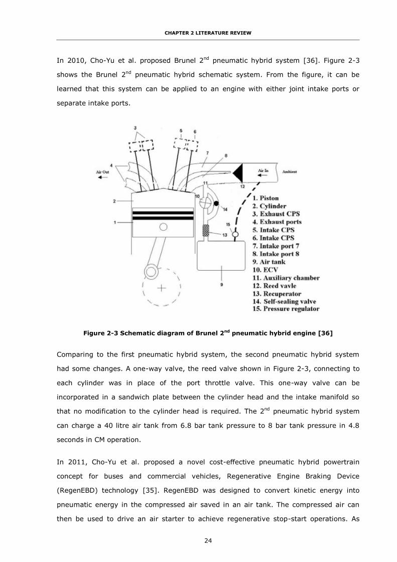
In 2010, Cho-Yu et al. proposed Brunel 2nd pneumatic hybrid system [36]. Figure 2-3
shows the Brunel 2nd pneumatic hybrid schematic system. From the figure, it can be
learned that this system can be applied to an engine with either joint intake ports or
separate intake ports.
Figure 2-3 Schematic diagram of Brunel 2nd pneumatic hybrid engine [36]
Comparing to the first pneumatic hybrid system, the second pneumatic hybrid system
had some changes. A one-way valve, the reed valve shown in Figure 2-3, connecting to
each cylinder was in place of the port throttle valve. This one-way valve can be
incorporated in a sandwich plate between the cylinder head and the intake manifold so
that no modification to the cylinder head is required. The 2nd pneumatic hybrid system
can charge a 40 litre air tank from 6.8 bar tank pressure to 8 bar tank pressure in 4.8
seconds in CM operation.
In 2011, Cho-Yu et al. proposed a novel cost-effective pneumatic hybrid powertrain
concept for buses and commercial vehicles, Regenerative Engine Braking Device
(RegenEBD) technology [35]. RegenEBD was designed to convert kinetic energy into
pneumatic energy in the compressed air saved in an air tank. The compressed air can
then be used to drive an air starter to achieve regenerative stop-start operations. As

CHAPTER 2 LITERATURE REVIEW
25
shown in Figure 2-4, a standard production air starter can be readily employed to crank
start the engine using the compressed air produced during the CM operation.
Figure 2-4 Schematic diagram of the air hybrid engine with an air starter [35]
The result showed that for a 151 litre air tank, it took 120 engine revolutions to charge
the air tank pressure from 4 bar to 6 bar (4.8 seconds at 1500 rpm engine speed). A
comparison of fuel consumption over the Millbrook London Transport Bus (MLTB) driving
cycle between the standard vehicle and air hybrid vehicle was given out. Standard
vehicle operation during the MLTB driving cycle consumed 3888.4 g of fuel. The
pneumatic hybrid vehicle used 3645.4 g of fuel, which represents a 6.2% reduction in
fuel consumption as a result of the regenerative stop-start operations [35].
2.3.3 ETH Zurich
Guzzella et al. proposed a pneumatic hybrid engine concept using an extra camless valve
connecting the cylinder and the air tank to eliminate the need for a complete set of fully
camless valves [40, 41]. As shown in the Figure 2-5, the intake and exhaust valves
remained camshaft-driven.
CHAPTER 2 LITERATURE REVIEW
26
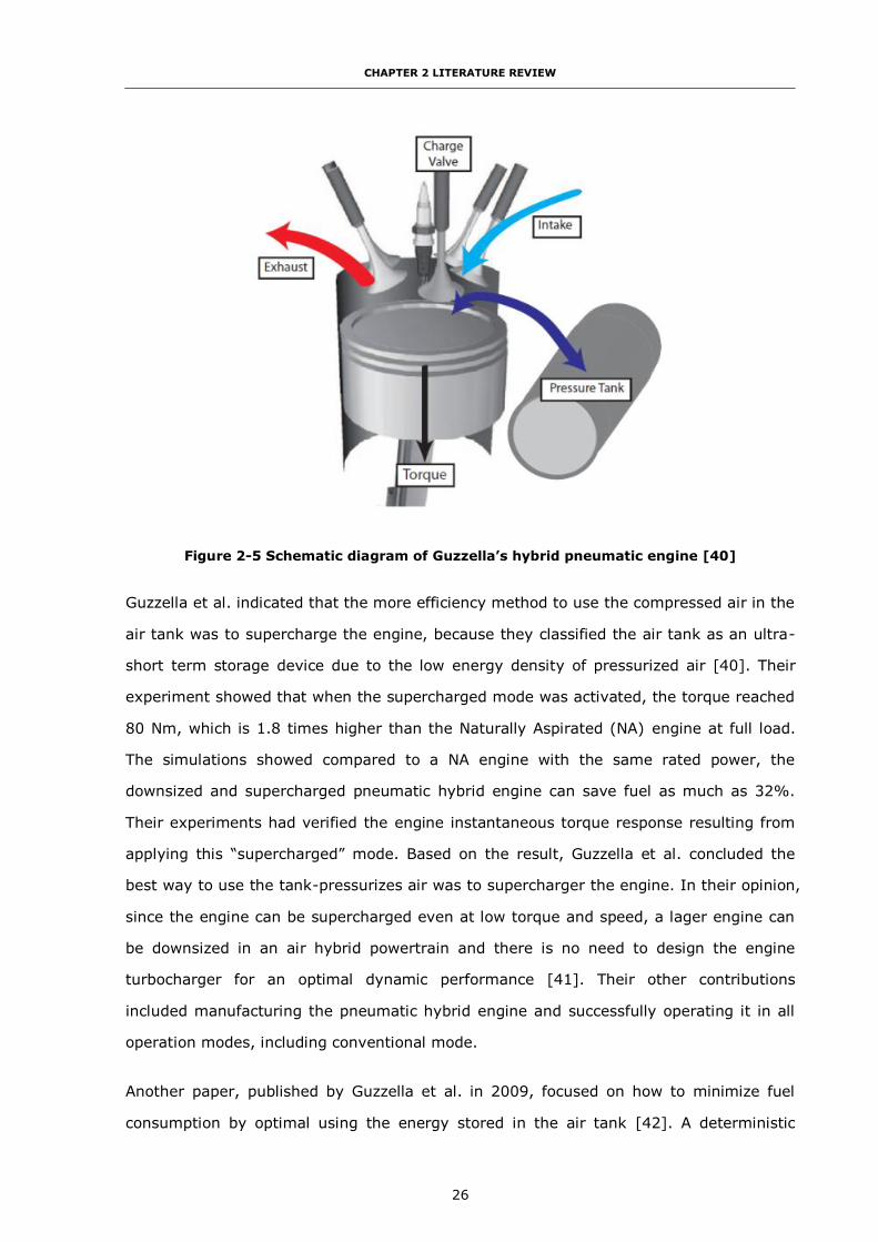
Figure 2-5 Schematic diagram of Guzzella’s hybrid pneumatic engine [40]
Guzzella et al. indicated that the more efficiency method to use the compressed air in the
air tank was to supercharge the engine, because they classified the air tank as an ultra-
short term storage device due to the low energy density of pressurized air [40]. Their
experiment showed that when the supercharged mode was activated, the torque reached
80 Nm, which is 1.8 times higher than the Naturally Aspirated (NA) engine at full load.
The simulations showed compared to a NA engine with the same rated power, the
downsized and supercharged pneumatic hybrid engine can save fuel as much as 32%.
Their experiments had verified the engine instantaneous torque response resulting from
applying this “supercharged” mode. Based on the result, Guzzella et al. concluded the
best way to use the tank-pressurizes air was to supercharger the engine. In their opinion,
since the engine can be supercharged even at low torque and speed, a lager engine can
be downsized in an air hybrid powertrain and there is no need to design the engine
turbocharger for an optimal dynamic performance [41]. Their other contributions
included manufacturing the pneumatic hybrid engine and successfully operating it in all
operation modes, including conventional mode.
Another paper, published by Guzzella et al. in 2009, focused on how to minimize fuel
consumption by optimal using the energy stored in the air tank [42]. A deterministic

CHAPTER 2 LITERATURE REVIEW
27
dynamic programming algorithm was implemented in this study to choose the mode of
engine operation at every time instant of the driving cycle while guaranteeing charge
sustenance. They concluded that the hybrid pneumatic engine concept based on fixed
camshafts combined with a downsized engine has the potential to be more cost-efficient
than fully variable hybrid pneumatic engines and hybrid electric propulsion systems.
Obtained result showed that the combination of engine downsizing and pneumatic
hybridization yields a fuel consumption reduction of up to 34% for the Motor Vehicle
Emissions Group (MVEG) driving cycle [42].
2.3.4 Lund Institute of Technology
In 2005, Andersson et al. proposed a new pneumatic hybrid concept which had two air
tanks [21]. The main difference between this novel pneumatic hybrid system and other
pneumatic hybrid concepts was using a pressure tank a the supplier of low air pressure
to instead of the atmosphere. By this modification, a very high torque can be achieved in
Compression Braking (CB) mode as well as in Air Motor (AM) mode. The proposed
configuration is shown in Figure 2-6.
Figure 2-6 Pneumatic hybrid concept using two tanks [21]
The authors reported for a city bus driven according to the Braunschweig driving cycle,
the reduction in fuel consumption is approximately 23%. Also, the simulations have
shown that a fairly high proportion (approximately 55%) of the shaft work absorbed by

CHAPTER 2 LITERATURE REVIEW
28
the engine during CB mode can be returned to the vehicle during acceleration in AM
mode.
In 2007, Trajkovic et al. in the same research group converted a Scania D12 single-
cylinder diesel engine to a pneumatic hybrid engine [46]. Pneumatic valve actuators
mounted on top of the cylinder head of the engine had been used to make the pneumatic
hybrid system possible. A pressure tank had been connected to one of the inlet ports and
one of the inlet valves had been modified to work as a tank valve. They tested and
studied two working mode, CB and AM and investigated the relationship between the
Engine’s Indicated Mean Effective Pressure (IMEP) and tank pressure with different valve
timings and engine speeds at the AM and CB. They reported the maximum regenerative
braking efficiency obtained in this study is 33% [46].
Trajkovic et al. published their second paper about the investigation on the same
pneumatic hybrid engine in 2008 [45]. This paper described the introduction of new tank
valve geometry to the system with the intent to increase the pneumatic hybrid
regenerative efficiency. The new tank valve has a larger valve head diameter than the
previously used setup described in [46], in order to decrease the pressure drop over the
tank valve. The total regenerative braking efficiency had been increased from 33% with
the small tank valve setup to 48% with the large tank valve setup, primarily due to a
larger valve head diameter and optimal valve timing.
Later in 2010, Trajkovic et al. conducted a vehicle driving cycle simulation of the
pneumatic hybrid [43]. The pneumatic hybrid powertrain had been modelled in GT-
POWER and validated against the experimental data to generate the pneumatic hybrid
powertrain performance maps. Based on the performance map, a driving cycle simulation
model had been developed in MATLAB/Simulink to evaluate the fuel consumption. They
reported that driving cycle simulations showed that fuel consumption can be reduced by
up to 30% over the Braunschweig driving cycle. However, only regenerative braking
accounts for about 10% of fuel consumption reduction, which corresponds to a
regenerative braking efficiency of about 20%. The remaining 20% of fuel consumption
reduction is due to stop-start functionality.

CHAPTER 2 LITERATURE REVIEW
29
2.3.5 University of Orléans
In 2002, Higelin et al. published a paper to present a new hybrid pneumatic-combustion
engine and the associated thermodynamic cycles [14]. The Pneumatic-hybrid
configuration is shown in Figure 2-7. From the figure, it can be seen that their concept
also had one additional valve, called the charging valve, connecting the combustion
chamber of each cylinder to an air tank. This valve’s opening and closing was driven by
an additional camshaft. The energy, stored in the form of compressed air, can be issued
from a braking phase or from a combustion phase at low power. The potential energy
from the air tank can then be restored to start the engine, or charge the engine at full
load. Higelin reported that regenerative breaking and the suppression of the idling
phases could provide an improvement in terms of fuel economy as high as 15% or more
if combined with engine downsizing.
Figure 2-7 Schematic diagram of Higelin’s hybrid pneumatic engine [14]
In 2004, Higelin et al. [19] published a paper to investigate the relationship between the
operation parameters and fuel consumption by using the same engine model developed
in [14]. They reported the global fuel consumption could be reduced by around 12%
without any specific optimisation. By optimizing the tank maximum allowed pressure, the
tank volume and the engine displacement, the global fuel economy during the driving
cycle could be further improved to 31% compared to conventional operation.

CHAPTER 2 LITERATURE REVIEW
30
In the paper Higelin et al. published at 2009, different energy management strategies for
hybrid pneumatic engine concept were proposed and compared [52]. They provided a
scale of the energy management strategies for the pneumatic hybrid engine working on
the real-time environment and leading to the close to optimal fuel saving. They reported
all strategies had provided significant fuel saving, and compared to the dynamic
programming, which required the perfect knowledge of the future pattern, also close to
optimal result [52]. It was also concluded that the strategy based on pattern recognition
with an associated variable pattern coefficient was the one with the lowest fuel
consumption, which was also the nearest of dynamic programming.
2.3.6 UCLA Research Group
In 2003, Tai et al. published a paper to describe the engine modifications,
thermodynamics of various operating modes and vehicle driving cycle simulation and
proposed a new pneumatic hybrid concept [17]. The engine design concept is illustrated
in Figure 2-8. This paper explored the fuel economy potential of an air hybrid engine in a
passenger car. It described the engine modifications, thermodynamic of various
operating modes and vehicle driving cycle simulation. Unlike other pneumatic hybrid
concept, in order to enable the air hybrid operation, two new systems had been
incorporated, a camless electrohydraulic valvetrain and intake air switching. The
modelling of the 1531 kg vehicle with the air hybrid engine resulted in fuel economy
improvement of 64% and 12% in city and highway driving respectively, compared to the
conventional baseline vehicle.
Figure 2-8 Schematic diagram of Tai’s hybrid pneumatic engine [17]
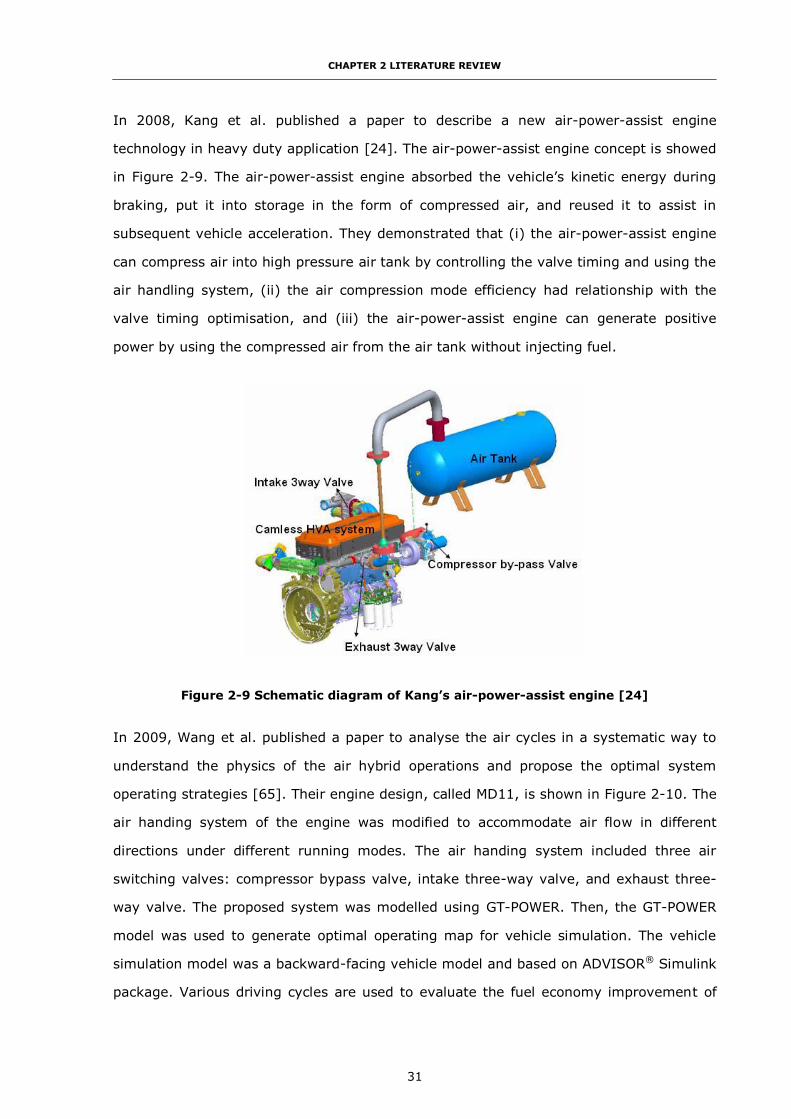
CHAPTER 2 LITERATURE REVIEW
31
In 2008, Kang et al. published a paper to describe a new air-power-assist engine
technology in heavy duty application [24]. The air-power-assist engine concept is showed
in Figure 2-9. The air-power-assist engine absorbed the vehicle’s kinetic energy during
braking, put it into storage in the form of compressed air, and reused it to assist in
subsequent vehicle acceleration. They demonstrated that (i) the air-power-assist engine
can compress air into high pressure air tank by controlling the valve timing and using the
air handling system, (ii) the air compression mode efficiency had relationship with the
valve timing optimisation, and (iii) the air-power-assist engine can generate positive
power by using the compressed air from the air tank without injecting fuel.
Figure 2-9 Schematic diagram of Kang’s air-power-assist engine [24]
In 2009, Wang et al. published a paper to analyse the air cycles in a systematic way to
understand the physics of the air hybrid operations and propose the optimal system
operating strategies [65]. Their engine design, called MD11, is shown in Figure 2-10. The
air handing system of the engine was modified to accommodate air flow in different
directions under different running modes. The air handing system included three air
switching valves: compressor bypass valve, intake three-way valve, and exhaust three-
way valve. The proposed system was modelled using GT-POWER. Then, the GT-POWER
model was used to generate optimal operating map for vehicle simulation. The vehicle
simulation model was a backward-facing vehicle model and based on ADVISOR® Simulink
package. Various driving cycles are used to evaluate the fuel economy improvement of

CHAPTER 2 LITERATURE REVIEW
32
the garbage refuse truck equipped with the air hybrid engine. The fuel economy
improvement ranged from 4% to 18% and it strongly dependent on the driving cycles.
Figure 2-10 MD11 air hybrid configuration [65]
2.3.7 Fuel Consumption Result Comparison and Analysis
Table 2-1 shows a comparison of result of the fuel consumption from different research
group. In this table, the different research results are not directly compared because of
different assumptions and constraints. But it still gives a rough overview of the
magnitude of the expected fuel savings. From the table, it can be seen that the total fuel
gains in the range of 4% to 50% can be expected depending on the vehicles and drive
cycles used. Also it demonstrates that most of the benefit may come from the engine
downsizing. This is because some research groups focus on using the pneumatic hybrid
technology to run the engine at air motor mode or air power assist mode. In these two
modes, the recover air in the air tank power the engine to start the engine alone or assist
the engine during the acceleration. As a result, the engine displacement can be
decreased to save fuel consumption. If only considering using the pneumatic hybrid
technology as a micro hybrid to realize the Stop-Start function, the fuel consumption
improvement is in the range of 6% to 20% depending on the vehicles and test cycles
used. In addition, some research group indicated that a part of fuel consumption

CHAPTER 2 LITERATURE REVIEW
33
reduction is due to the increased transmission efficiency caused by the possibility to
operate the engine at very low rotational speed in CB and AM mode.
Table 2-1 Summary table of fuel consumption result
Research Group
Year Engine Vehicle Tank Size
Maximum
Tank
Pressure
Fuel
Consumption
Reduction
Test cycle
Michael M. Schechter
1999 2 l
Gasoline
1360 kg
Car
36.2 l
-
Total 50%
45 s city driving cycle
Stop-Start -
Engine
Downsizing -
Brunel University
London
2011 7.25 l
Diesel
16500 kg
Bus
151 l 10 bar
Total 6.2%
MLTB Stop-Start 6.2%
Engine
Downsizing 0
ETH Zurich 2009 2 l
Gasoline
1450 kg
Car 30 l 24.2 bar
Total 34%
MVEG-95 Stop-Start 6%
Engine
Downsizing 28%
Lund
University 2005
11.7 l
Diesel
15000
kg
Bus
143 l - Total 23%
Braunschweig 600 l -
Stop-Start -
Engine Downsizing
-
Lund
University 2010
12 l
Diesel
15000
kg
Bus
40 l 27 bar
Total 28%
Braunschweig Stop-Start 20%
Engine Downsizing
-
University
of Orléans 2003
2 l
Gasoline
800 kg
Car 50 l 20 bar
Total 31%
NEDC Stop-Start -
Engine
Downsizing -
UCLA 2003 2.5 l 1531 kg
Car 65 l 24 bar
Total -
FTP City 64%
Highway 12%
UCLA 2008 10.8 l Garbage refuse
truck
280 l 15 bar
Total 4-
18% Different test
cycles Stop-Start -
Engine
Downsizing -
2.4 Summary
In this chapter, a literature view about the pneumatic hybrid engine concepts was
presented. By summarizing the research before, it can be learned that there are several
research topics are not investigated or deeply studied before:

CHAPTER 2 LITERATURE REVIEW
34
(i) Thermodynamic analysis of the operation of the pneumatic hybrid engine to
supply an understanding of the sensitivity of the work done to design parameters.
(ii) How to implement the pneumatic hybrid powertrain to an appropriate braking
system to maximize the energy recovery efficiency during braking.
(iii) Understanding of the contribution of the pneumatic hybrid powertrain to vehicle
braking and how the braking effect in alongside friction braking.
(iv) Understanding of the contribution to fuel economy and performance made by the
development of pneumatic assistant in accelerating the turbocharger.
(v) Detailed investigating how to reduce turbo-lag and improve engine transient
response by pneumatic hybrid technology.
(vi) Using forward-facing simulation to evaluate the fuel economy improvement by
pneumatic hybrid technology.
(vii) Develop a pneumatic hybrid vehicle control algorithm to realize the energy
storage and regeneration as well as the normal operation of the vehicle.
(viii) Identify the relationship between hybrid powertrain operating parameters, fuel
consumption and energy usage according to optimisation criteria.
The research topics above have been detailed investigated in this research. Topic (i) has
been investigated in Chapter3. Topic (ii-iii) has been studied in Chapter 5. Topic (iv-v)
has been analysed in Chapter 6. And Topic (vi-viii) has been researched in Chapter 7.
CHAPTER 3 PRINCIPLES OF PENUMATIC HYBRID ENGINE
35
CHAPTER 3
PRINCIPLES OF PENUMATIC HYBRID ENGINE
3.1 Introduction
This investigation into the pneumatic hybrid concept is based on the YUCHAI YC6A diesel
engine. The intention of this chapter is to present the principles of operation and to
confirm the potential of the new systems to both generate a supply of compressed air
and to manage the contribution of the engine to vehicle braking.
The Chapter is arranged as follows:
(i) The engine and a series of proposed modifications are described in detail to
explain the pneumatic hybrid engine operating process.
(ii) The pneumatic hybrid engine CM is considered from a theoretical perspective
based on an air cycle analysis.
(iii) Based on this analysis, the implementation of a single cylinder model in CM
operation is described and demonstrated. The model is validated by means of an
independently developed model using the GT-POWER engine simulation code.
(iv) Results from the model show the effect of respectively the air tank pressure,
engine speed, intake valve second opening time and actual compression ratio
are studied using the model. (Note that the actual compression ratio Rc decrease
from the geometric compression ratio as the volume of the auxiliary chamber is
included in the cylinder’s total clearance volume when the engine is in CM.)
3.2 Pneumatic Hybrid Engine Concept
3.2.1 Configuration of the Pneumatic Hybrid Engine
The YUCHAI YC6A six cylinders 7.25 l diesel engine commonly used in passenger bus and
freight vehicle applications provides the engine technology context for the work that is
the basis of this thesis. The YC6A engine is a typical engine in this class and it has no

CHAPTER 3 PRINCIPLES OF PENUMATIC HYBRID ENGINE
36
doubt that the results derived from this engine can be extended to other medium and
heavy duty engines. Figure 3-1 shows a schematic diagram of this engine. A split intake
port provides a flow path to the air tank. In normal operating mode, a Throttle Valve (TV)
located in the intake port will be fully opened. Air flows through the intake valves via
separate intake ports during the intake stroke and leaves exhaust ports during the
exhaust stroke. One of the intake valves is equipped with a Compression Release Engine
Braking (CREB) device normally used on the exhaust valve for the purpose of engine
braking [34], named CREB intake valve here. When the vehicle brakes and the CM is
selected, fuel supply is cut. With the clutch engaged, the engine has now become a
compressor to provide regenerative braking to recover the energy by converting a
proportion of the vehicle kinetic energy to the internal energy of pressurised air in the air
tank.
Figure 3-1 Schematic diagram of the pneumatic hybrid engine
In CM operation, during the compression stroke, the CREB intake valve is opened and the
air is compressed into the intake port. At the same time, the throttle valve is fully closed
to prevent compressed air escaping into the intake manifold. The Check Valve (CV) which
seals the air tank will open when the intake manifold pressure is higher than the tank

CHAPTER 3 PRINCIPLES OF PENUMATIC HYBRID ENGINE
37
pressure. The air will be compressed into the air tank. The air tank has the same
construction as the standard one on commercial vehicles or buses with a peak pressure
of 10 bar which is limited to this value for safety reasons. The auxiliary chamber is a
small chamber which accommodates the CREB intake valve, CV and TV. All engine
cylinders are equipped with the same valves and porting as shown in Figure 3-1. The
engine and the pneumatic hybrid system main technical parameters are summarized in
Table 3-1.
Table 3-1 Main technical parameters of the engine and pneumatic hybrid system
Displacement (l) 7.25
Electronic control system High pressure & common rail
No. of Cylinders (-) 6
Bore (mm) 108
Stroke (mm) 132
Compression ratio (-) 17.5:1
Intake way Turbo-charging & inter-cooling
Rated power/speed (kW/rpm) 177/2300
Max torque/speed (Nm/rpm) 900/1400~1600
Intake valve (-) 2
Diameter (mm) 32.5
Opening point (normal) 61°BTDC
Closing point (normal) 91°ABDC
Exhaust valve (-) 2
Diameter (mm) 29.5
Opening point (normal) 105°BBDC
Closing point (normal) 67°ATDC
Air tank volume (l) 151
In this research, the air tanks are uninsulated. A simulation is conducted by Lee et.al to
compare the air tank temperature change between an insulated air tank and an
uninsulated air tank using the same engine used here [34]. The result is shown in Figure

CHAPTER 3 PRINCIPLES OF PENUMATIC HYBRID ENGINE
38
3-2. It shows the compressed air temperature in an insulated air tank and an uninsulated
air tank against engine revolutions. In the case of an insulated air tank, the zero value of
the wall heat transfer is applied to assume it is in adiabatic condition. From Figure 3-2, it
can be seen that the compressed air reaches 795 K after a charging process of 800
engine revolutions at 1500 rpm in the insulation air tank. In the normal tank without
insulation, the compressed air temperature reaches the ambient temperature after 1200
engine revolutions at same engine speed.
Figure 3-2 Tank temperatures for 1500 r/min engine speed [34]
Lee et.al also evaluated the air tank temperature for the pneumatic hybrid engine by
comparing the experimental and predicted results [4]. The 13 l air tank was charged at
1500 rpm for 700 engine revolutions. The result is shown in Figure 3-3. It indicates that
the difference between the experimental and predicted temperature is less than 5 K.
In fact, it would be ideal to store both the pneumatic and thermal energy in the form of
hot compressed air in an adiabatic air tank or through a heat recuperator. The hot
compressed air can then be used to restart the engine [34]. However, the maximum
operating temperature of the current air starter is limited to 100°C [34]. Therefore, in
the subsequent research, the pneumatic hybrid powertrain will be modelled with an
uninsulated air tank in order to produce more realistic results.

CHAPTER 3 PRINCIPLES OF PENUMATIC HYBRID ENGINE
39
Figure 3-3 Experimental and predicted air tank temperature at 1500 r/min engine speed
for 700 engine cycles [4]
3.2.2 Principle of Operation
Figure 3-4 shows the valve timing diagram for the normal mode and CM. During the
normal mode, the CREB intake valve operates as an intake valve whose lift profile is
exactly the same as another intake valve of the same cylinder. In order to keep the air
flow rate in the intake manifold as high as possible, the throttle valve is always opened to
its maximum value during normal operation.
During vehicle deceleration and braking, the engine becomes a compressor and no fuel is
injected into the cylinders. In all cylinders, intake valves are opened to let the air into the
cylinder during the intake stroke. Then the normal intake valve is closed and as the
piston passes Bottom Dead Centre (BDC) and would normally begin the compression
stroke, the CREB intake valve opens to allow air to enter the auxiliary chamber. At the
same time, the throttle valve is closed and the check valve opened. Air is compressed
into the air tank.
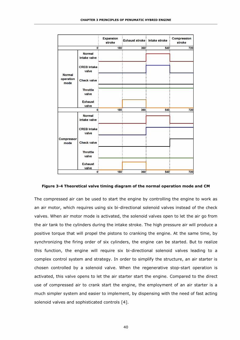
CHAPTER 3 PRINCIPLES OF PENUMATIC HYBRID ENGINE
40
Figure 3-4 Theoretical valve timing diagram of the normal operation mode and CM
The compressed air can be used to start the engine by controlling the engine to work as
an air motor, which requires using six bi-directional solenoid valves instead of the check
valves. When air motor mode is activated, the solenoid valves open to let the air go from
the air tank to the cylinders during the intake stroke. The high pressure air will produce a
positive torque that will propel the pistons to cranking the engine. At the same time, by
synchronizing the firing order of six cylinders, the engine can be started. But to realize
this function, the engine will require six bi-directional solenoid valves leading to a
complex control system and strategy. In order to simplify the structure, an air starter is
chosen controlled by a solenoid valve. When the regenerative stop-start operation is
activated, this valve opens to let the air starter start the engine. Compared to the direct
use of compressed air to crank start the engine, the employment of an air starter is a
much simpler system and easier to implement, by dispensing with the need of fast acting
solenoid valves and sophisticated controls [4].

CHAPTER 3 PRINCIPLES OF PENUMATIC HYBRID ENGINE
41
The size of the auxiliary chamber of this engine, is an important design parameter that
affects the efficiency of the CM. The size of this chamber depends on the positions of the
CV and TV [10]. The compression ratio of this engine changes when working in CM
because of the additional volume of the auxiliary chamber is added in. The actual
compression ratio Rc of CM for the engine using in this research is calculated by Lee et al.
which is 5.3:1 [10]. In the later section, how the actual compression ratio affecting the
CM performance will be discussed in detail.
3.3 Pneumatic Hybrid Engine Compressor Mode
During vehicle braking, when the CM is activated, the engine operates as a compressor
driven from the wheels by vehicle motion and pumping compressed air into the air tank.
Work done by the pistons causes the vehicle to decelerate, converting a proportion of its
kinetic energy into the energy of compressed air. To fully understand the physics of the
CM operation, the thermodynamic cycle of a one cylinder engine will be described and
analysed. Based on the analysis, engine performance, brake torque, air tank pressure
and valves timing can be calculated as a function of engine speed.
3.3.1 Theoretical Analysis of the Pneumatic Hybrid Engine Compressor
Mode
Unlike most pneumatic hybrid engines that operate two strokes to recover the energy
during the air compress mode [63, 65], the pneumatic hybrid engine used in this
research continues to follow four-stroke operation during CM. The four strokes in CM are
Intake Stroke, Compression Stroke, Expansion Stroke and Exhaust Stroke. Figure 3-5
illustrates the ideal p-V (pressure-volume) diagram of this cycle, which shows the
pressure variation in the cylinder as a function of the piston position. In this diagram, Vs
is the cylinder swept volume, Vc is the cylinder clearance volume, Vaux is the volume of
the auxiliary chamber, p0 is the pressure of the intake manifold, and pt is the air tank
pressure.

CHAPTER 3 PRINCIPLES OF PENUMATIC HYBRID ENGINE
42
Figure 3-5 Ideal p-V diagram during the CM
The following assumptions simplify the analysis process without undermining the
accuracy.
(i) Valves open and close instantaneously. (Valves moving speed is fast compared
with piston motion.)
(ii) Filling and emptying proceeds rapidly to equilibrium without losses. (At normal
operation speed, gas flow is rapid compared with position motion.)
(iii) Intake and exhaust pressure constant during valve events. (Both pressures vary
slightly compared with variation of cylinder pressure.)
Compression Stroke
The Compression Stroke (1-5) comprises four distinct stages during piston movement
from BDC to Top Dead Centre (TDC).
Stage 1-2: Starting with the piston at BDC (point 1), finishing with the inlet valves open
(point 2). From point 1 to point 2, the intake valves and exhaust valves are all fully
closed as shown in the Figure 3-6. The piston on its rising stroke will compress the air
and the pressure in the cylinder increases. (Note that the CREB intake valve opens at
point 2.)

CHAPTER 3 PRINCIPLES OF PENUMATIC HYBRID ENGINE
43
Figure 3-6 Schematic diagram of the start of the Compression Stroke in CM
Stage 2-3: The CREB intake valve opens again at point 2, while the CV and the TV are
closed, as shown in Figure 3-7. At this point, the working volume is increased by the
additional volume of the auxiliary chamber. Because before the CREB intake valve second
open, the pressure in the auxiliary chamber is constant. Furthermore, it is assumed that
the valve open instantaneously. As a result, at the CREB intake valve opening point, the
pressure of the cylinder is higher than the pressure of the auxiliary chamber. Once the
CREB intake valve open, the high pressure air in the cylinder flow to the auxiliary
chamber which cause a pressure drop from point 2 to point 3. It is shown on the p-V
diagram as an increase in volume and a decrease in pressure. In fact, it should always
keep the air pressurized during the work stroke. But the CREB intake valve cannot be
always open. Furthermore, although the pressure is drop, the CREB intake valve open
again increase the air mass being compressed. This is because the air in the auxiliary
chamber is added to be compressed by the piston.
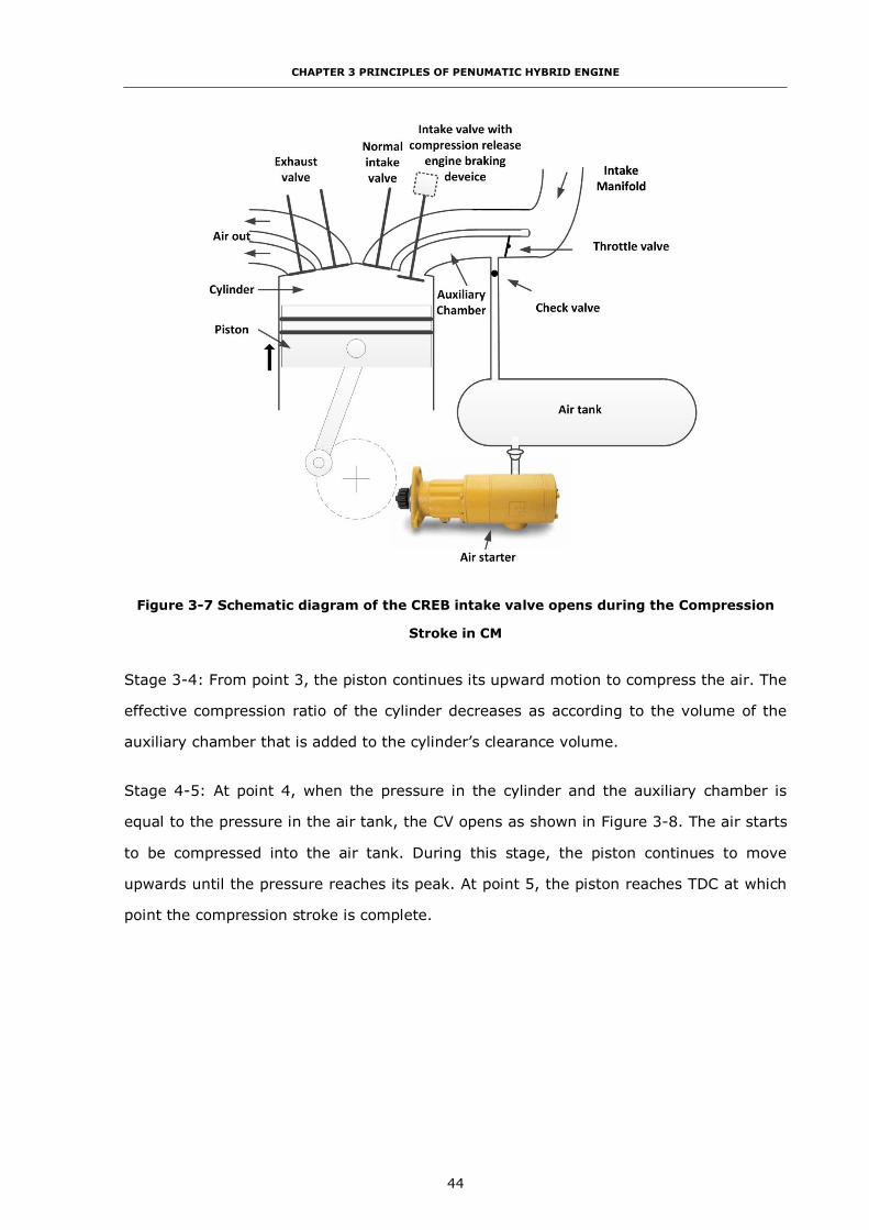
CHAPTER 3 PRINCIPLES OF PENUMATIC HYBRID ENGINE
44
Figure 3-7 Schematic diagram of the CREB intake valve opens during the Compression
Stroke in CM
Stage 3-4: From point 3, the piston continues its upward motion to compress the air. The
effective compression ratio of the cylinder decreases as according to the volume of the
auxiliary chamber that is added to the cylinder’s clearance volume.
Stage 4-5: At point 4, when the pressure in the cylinder and the auxiliary chamber is
equal to the pressure in the air tank, the CV opens as shown in Figure 3-8. The air starts
to be compressed into the air tank. During this stage, the piston continues to move
upwards until the pressure reaches its peak. At point 5, the piston reaches TDC at which
point the compression stroke is complete.
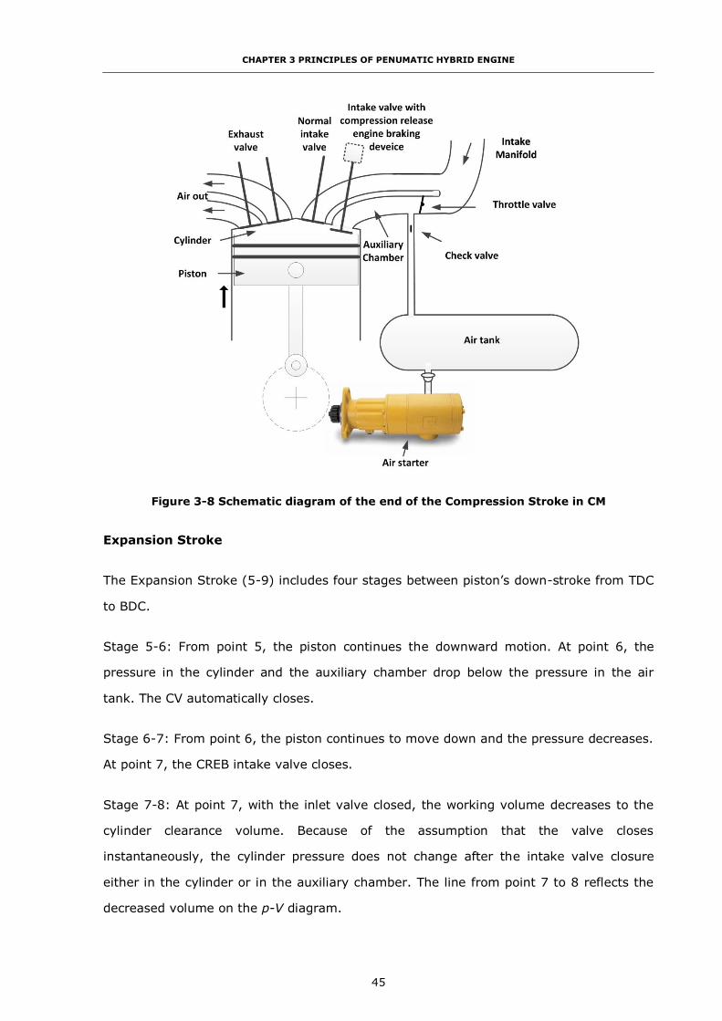
CHAPTER 3 PRINCIPLES OF PENUMATIC HYBRID ENGINE
45
Figure 3-8 Schematic diagram of the end of the Compression Stroke in CM
Expansion Stroke
The Expansion Stroke (5-9) includes four stages between piston’s down-stroke from TDC
to BDC.
Stage 5-6: From point 5, the piston continues the downward motion. At point 6, the
pressure in the cylinder and the auxiliary chamber drop below the pressure in the air
tank. The CV automatically closes.
Stage 6-7: From point 6, the piston continues to move down and the pressure decreases.
At point 7, the CREB intake valve closes.
Stage 7-8: At point 7, with the inlet valve closed, the working volume decreases to the
cylinder clearance volume. Because of the assumption that the valve closes
instantaneously, the cylinder pressure does not change after the intake valve closure
either in the cylinder or in the auxiliary chamber. The line from point 7 to 8 reflects the
decreased volume on the p-V diagram.
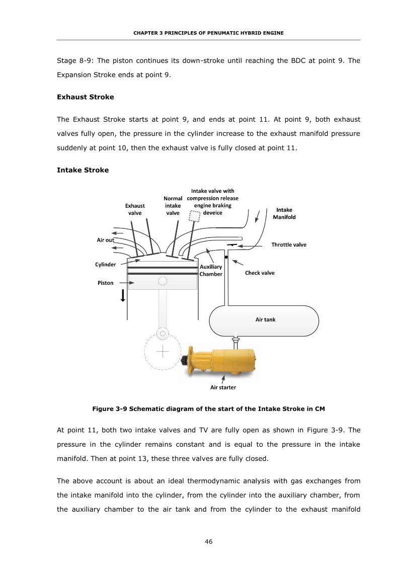
CHAPTER 3 PRINCIPLES OF PENUMATIC HYBRID ENGINE
46
Stage 8-9: The piston continues its down-stroke until reaching the BDC at point 9. The
Expansion Stroke ends at point 9.
Exhaust Stroke
The Exhaust Stroke starts at point 9, and ends at point 11. At point 9, both exhaust
valves fully open, the pressure in the cylinder increase to the exhaust manifold pressure
suddenly at point 10, then the exhaust valve is fully closed at point 11.
Intake Stroke
Figure 3-9 Schematic diagram of the start of the Intake Stroke in CM
At point 11, both two intake valves and TV are fully open as shown in Figure 3-9. The
pressure in the cylinder remains constant and is equal to the pressure in the intake
manifold. Then at point 13, these three valves are fully closed.
The above account is about an ideal thermodynamic analysis with gas exchanges from
the intake manifold into the cylinder, from the cylinder into the auxiliary chamber, from
the auxiliary chamber to the air tank and from the cylinder to the exhaust manifold

CHAPTER 3 PRINCIPLES OF PENUMATIC HYBRID ENGINE
47
taking place in a reversible manner. In practice, this can never be realised, but sets an
ideal against which actual performance can be judged.
If only the pressure in the cylinder is considered, the p-V diagram will transform to the
diagram shown in Figure 3-10. In Figure 3-10, the solid line indicates the pressure
change in the cylinder, while the dashed line shows the pressure variation in the volume
that additionally includes the auxiliary chamber. From Figure 3-10, at point 4 when the
check valve opens, because of the pressure drop of the CV, the pressure in the cylinder
cannot be equal to the pressure in the air tank. As a result, the pressure in the cylinder
continues to rise up as the piston goes up until TDC. Point 5 shows the upper bound of
the pressure variation at the end of the position rising up stroke which is the maximum
pressure can be achieved.
Figure 3-10 Modified p-V diagram during the CM
Based on cycle shown in Figure 3-10, the thermodynamic analysis of the CM, where the
control volume is bounded by the piston, cylinder walls and the auxiliary chamber is
shown in Figure 3-11, is presented in the next section of this Chapter.
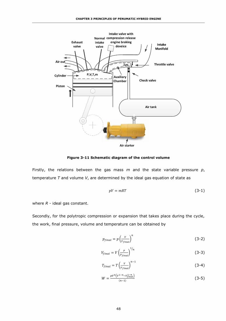
CHAPTER 3 PRINCIPLES OF PENUMATIC HYBRID ENGINE
48
Figure 3-11 Schematic diagram of the control volume
Firstly, the relations between the gas mass m and the state variable pressure p,
temperature T and volume V, are determined by the ideal gas equation of state as
𝑝𝑉 = 𝑚𝑅𝑇 (3-1)
where R - ideal gas constant.
Secondly, for the polytropic compression or expansion that takes place during the cycle,
the work, final pressure, volume and temperature can be obtained by
𝑝𝑓𝑖𝑛𝑎𝑙 = 𝑝 (𝑉
𝑉𝑓𝑖𝑛𝑎𝑙)
𝑛
(3-2)
𝑉𝑓𝑖𝑛𝑎𝑙 = 𝑉 (𝑃
𝑃𝑓𝑖𝑛𝑎𝑙)
1𝑛⁄
(3-3)
𝑇𝑓𝑖𝑛𝑎𝑙 = 𝑇 (𝑉
𝑉𝑓𝑖𝑛𝑎𝑙)
𝑛−1
(3-4)
𝑊 =𝑝𝑉𝑛(𝑉1−𝑛−𝑉𝑓𝑖𝑛𝑎𝑙
1−𝑛 )
(𝑛−1) (3-5)

CHAPTER 3 PRINCIPLES OF PENUMATIC HYBRID ENGINE
49
where pfinal – final pressure,
p – initial pressure,
V – initial volume,
Vfinal – final volume,
W – work done during the compression or expansion,
n – polytropic index.
Thirdly, for the final volume of polytropic compression like stage 1-2, can be obtained by
𝑉𝑓𝑖𝑛𝑎𝑙 =(𝐷−𝐼𝑉𝑆𝐶)𝑉
180+
(180+𝐼𝑉𝑆𝐶−𝐷)𝑉𝑐
180 (3-6)
where D – duration of the CREB intake valve second opening in crank angle,
IVSC – CREB Intake Valve Second Close (IVSC) time after TDC,
V – initial volume,
Vc – cylinder clearance volume.
This is because, at point 2, the CREB intake valve opens again to let the air start to be
compressed into the auxiliary chamber which is governed by the intake valve second
opening timing.
For the compression stage 4-5, because of the check valve open, the air is compressed
into the air tank through the check valve. The air flow through the check valve can be
obtained by
�̇� = 𝑐𝑑𝐴√2𝜌√𝑝𝑖𝑛 − 𝑝𝑜𝑢𝑡 (3-7)
where �̇� – mass flow through the valve,
A – open area of the valve,
Cd – discharge coefficient,
ρ – density of the air,
pin – pressure upstream of the valve
pout – pressure downstream of the valve.
The mass remained in the control volume can be expressed as
𝑚5 = 𝑚4 − �̇�𝑡 (3-8)

CHAPTER 3 PRINCIPLES OF PENUMATIC HYBRID ENGINE
50
where m5 – air mass at point 5,
m4 – air mass at point 4,
�̇� – mass flow through the valve,
t – time that check valve open.
Then, for the stage 2-3 and 9-10, because the valve is assumed to be ideal which opens
instantaneously, these two expansions can be considered as a constant-volume process.
The work done by these two stages is equal 0.
For the stage 10-11 and 12-13, because it assumed that the air filling into and
discharging from the cylinder to the exhaust and intake system reaches equilibrium
rapidly and without loss, these two stages can be considered as an isobaric process. The
work done on the system by the piston during these two stages can be obtained by
𝑊 = 𝑝(𝑉𝑓𝑖𝑛𝑎𝑙 − 𝑉) (3-9)
Finally, the indicated work Wc,i done by the piston on the gas during one engine cycle in
one cylinder is
𝑊𝑐,𝑖 = ∮ 𝑝 𝑑𝑉 (3-10)
If it is assumed that the pressure recorded by the indicator diagram is the same as the
pressure which acts on the piston face [66]. Here, the indicated work Wc,i is equal to the
total of the work done in the each stage:
𝑊𝑐,𝑖 = 𝑊1−2 + 𝑊2−3 + 𝑊3−4 + 𝑊4−5 + 𝑊5−6 + 𝑊6−7 + 𝑊7−8
+𝑊8−9 + 𝑊9−10 + 𝑊10−11 + 𝑊11−12 + 𝑊12−13 (3-11)
Based on Equations (3-1) to (3-11), the indicated work for the cycle Wc,i can be
calculated.
IMEP (pmi) is a measure of the indicated work output per unit swept volume of one
cylinder (Vc,h), in a form independent of engine size and engine speed.
𝑝𝑚𝑖 =𝑊𝑐,𝑖
𝑉𝑐,ℎ (3-12)
The indicated power Pi of the engine is

CHAPTER 3 PRINCIPLES OF PENUMATIC HYBRID ENGINE
51
𝑃𝑖 =𝑝𝑚𝑖𝑉𝑐,ℎ𝑖𝑁
𝑛𝑅 (3-13)
where nR – number of the crank revolutions for each power stroke per cylinder which 1
for two-stroke and 2 for four-stroke engines,
i – number of the cylinders,
N – engine speed.
The effective power differs from the indicated power essentially in the frictional losses
(piston, bearings), the power-transmission losses from the control elements (camshaft,
valves), and the power of the accessories (oil, water and fuel injection pumps, alternator).
For the mechanical efficiency:
𝜂𝑚 =𝑃𝑒
𝑃𝑖 (3-14)
where Pe – measured power output.
Normal mechanical efficiencies are load-dependent and at full load are typically about
90%, while at low part load (10% load) about 70% [67]. Therefore, the measured power
of the engine is
𝑃𝑒 = 𝑃𝑖𝜂𝑚 (3-15)
Hence, the brake torque T is:
𝑇 =60∙1000
2𝜋
𝑃𝑒
𝑁=
9549𝑃𝑒
𝑁 (3-16)
Here, the brake torque of the engine during the vehicle braking can be calculated out.
3.3.2 Pneumatic Hybrid Engine Compressed Mode Model Validation and
Performance Analysis
3.3.2.1 Model Validation
Based on the theoretical analysis above, a program in Matlab, called Theoretical model
here, which can simulate the performance of the engine CM under different conditions, is
coded and introduce in Appendix-I. To validate the theoretical model, the result of a one
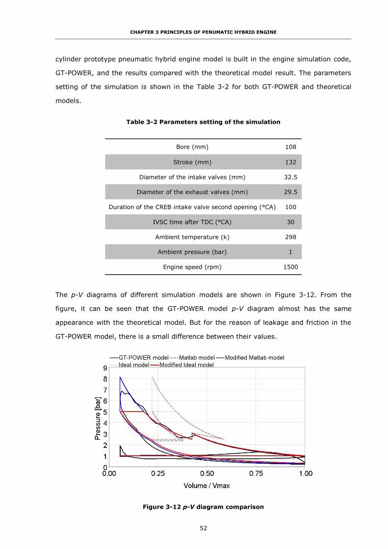
CHAPTER 3 PRINCIPLES OF PENUMATIC HYBRID ENGINE
52
cylinder prototype pneumatic hybrid engine model is built in the engine simulation code,
GT-POWER, and the results compared with the theoretical model result. The parameters
setting of the simulation is shown in the Table 3-2 for both GT-POWER and theoretical
models.
Table 3-2 Parameters setting of the simulation
Bore (mm) 108
Stroke (mm) 132
Diameter of the intake valves (mm) 32.5
Diameter of the exhaust valves (mm) 29.5
Duration of the CREB intake valve second opening (°CA) 100
IVSC time after TDC (°CA) 30
Ambient temperature (k) 298
Ambient pressure (bar) 1
Engine speed (rpm) 1500
The p-V diagrams of different simulation models are shown in Figure 3-12. From the
figure, it can be seen that the GT-POWER model p-V diagram almost has the same
appearance with the theoretical model. But for the reason of leakage and friction in the
GT-POWER model, there is a small difference between their values.
Figure 3-12 p-V diagram comparison

CHAPTER 3 PRINCIPLES OF PENUMATIC HYBRID ENGINE
53
To generate the engine response map, the GT-POWER model and the theoretical model
are running the steady-state simulation respectively. The results are shown in Table 3-3
and Table 3-4.
Table 3-3 Theoretical model engine brake torque (Nm) map
Engine speed (rpm)
500 1000 1500 2000
Air tank
pressure (bar)
4 -21.0692 -23.1357 -24.9664 -26.8605
5 -19.8087 -21.5004 -23.1762 -24.9868
6 -18.1194 -19.6078 -21.2043 -22.973
7 -16.1869 -17.5763 -19.1357 -20.8852
8 -14.1173 -15.4694 -17.0154 -18.758
Table 3-4 GT-POWER model engine brake torque (Nm) map
Engine speed (rpm)
500 1000 1500 2000
Air tank
pressure
(bar)
4 -18.1272 -20.7343 -23.153 -25.5917
5 -17.009 -19.497 -21.9799 -24.5333
6 -15.5407 -18.0149 -20.5717 -23.31
7 -13.9945 -16.3552 -19.0587 -21.9298
8 -13.9564 -16.3042 -18.8979 -21.6776
From the two tables above and Figure 3-15, it can be seen that when the engine speed
increases, the brake torque increases. Conversely, at constant engine speed as air tank
pressure increases, the brake torque decreases. It can be seen that the difference
between the GT-POWER model and the theoretical model falls as the engine speed
increases. The result also indicates that the thermodynamic model can be used to
calculate the engine brake torque in CM and is sufficiently reliable to be used for the
analysis of the engine performance of CM.

CHAPTER 3 PRINCIPLES OF PENUMATIC HYBRID ENGINE
54
Figure 3-13 shows that the in-cylinder pressure, auxiliary chamber pressure and the air
tank pressure during one engine cycle of the GT-POWER model. It can be seen that in-
cylinder pressure rises after both intake valves close after BDC and the pressure in the
auxiliary chamber increases immediately after the CREB intake valve second opening.
Both pressures remain the same during the opening period of the CV near TDC when the
auxiliary chamber pressure becomes higher than the air tank pressure. After TDC, the air
flow stops when the auxiliary chamber pressure is lower than the air tank pressure. After
that, the auxiliary chamber pressure remains constant until the intake valves open again
in the next cycles.
Figure 3-13 Pressure diagram in the CM
3.3.2.2 Performance Analysis
Figure 3-14 shows the p-V diagrams for various air tank pressures at 1500 rpm
simulated by the theoretical model. The figure indicates that different air tank pressure
can cause different engine brake torque performance during the CM. It can be seen that
the lower air tank pressure can create more brake torque which is shown in Figure 3-14
as the biggest area surrounded by the red line. The 7 bar air tank pressure lead the
lowest brake torque which has the smallest area p-V diagram. This is because the lower
air tank pressure causes an earlier check valve open time which resulting in long piston
working time. Thus, the engine brake torque is a function of tank pressure.
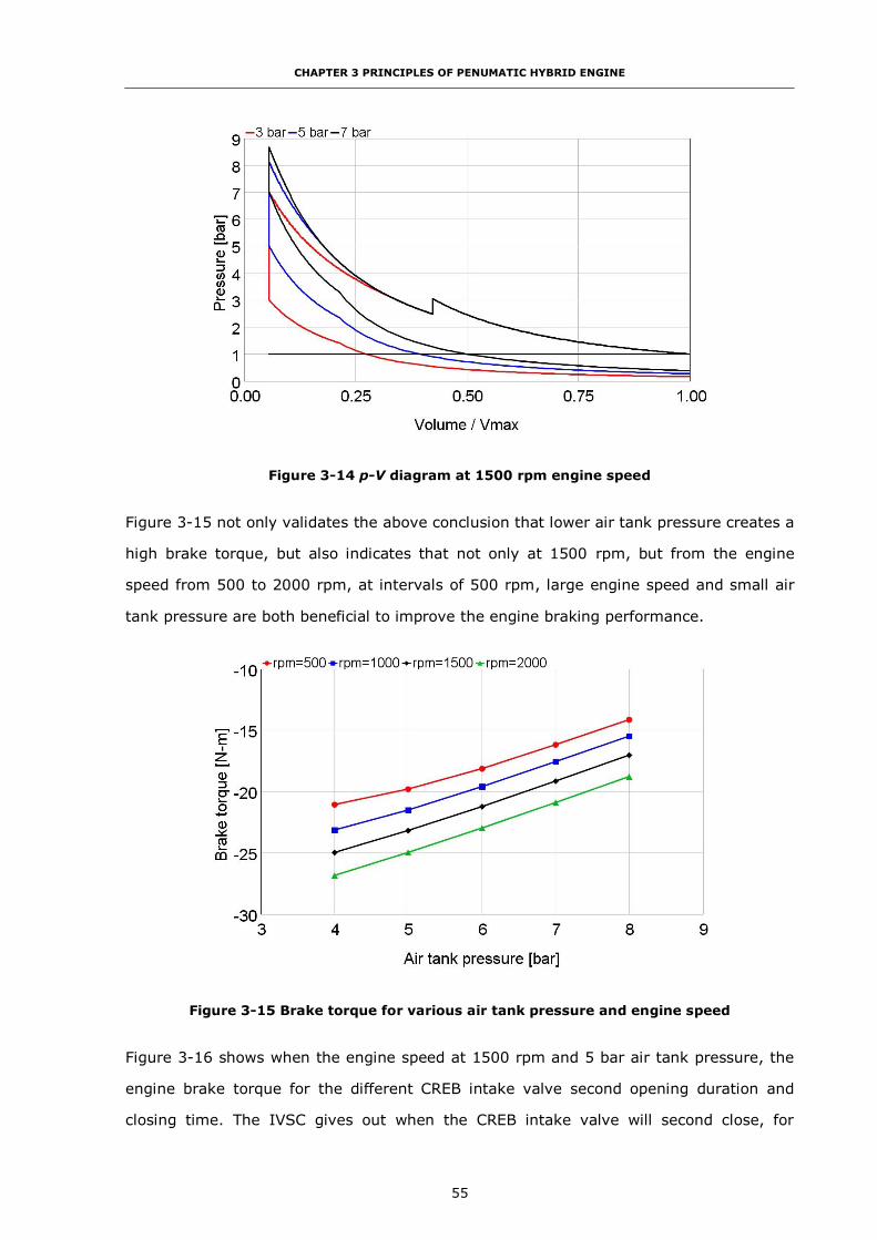
CHAPTER 3 PRINCIPLES OF PENUMATIC HYBRID ENGINE
55
Figure 3-14 p-V diagram at 1500 rpm engine speed
Figure 3-15 not only validates the above conclusion that lower air tank pressure creates a
high brake torque, but also indicates that not only at 1500 rpm, but from the engine
speed from 500 to 2000 rpm, at intervals of 500 rpm, large engine speed and small air
tank pressure are both beneficial to improve the engine braking performance.
Figure 3-15 Brake torque for various air tank pressure and engine speed
Figure 3-16 shows when the engine speed at 1500 rpm and 5 bar air tank pressure, the
engine brake torque for the different CREB intake valve second opening duration and
closing time. The IVSC gives out when the CREB intake valve will second close, for

CHAPTER 3 PRINCIPLES OF PENUMATIC HYBRID ENGINE
56
example, ‘IVSC=0’ means the CREB intake valve second closing happens at piston
exactly reaches the TDC; ‘IVSC=10’ means it will close at 10° CA after the piston reaches
TDC. The duration means the time that the CREB intake valve second opening will last. A
larger number of duration means a long second opening time of the CREB intake valve.
From the figure, it can be learned that, if the CREB intake valve closing time after TDC is
fixed, the longer second open duration decreases the brake torque performance of the
engine. In other words, it means earlier second open the CREB intake valve during the
piston upstroke, resulting in lower brake torque. The reason is when the CREB intake
valve second opens, the cylinder connects the auxiliary chamber resulting in an increased
volume and decrease the compression ratio which leads the cylinder pressure cannot be
compressed to high pressure, as a result, the low braking performance.
Figure 3-16 Brake torque for different intake timings
The figure also shows that the CREB intake valve closure after TDC can affect the engine
brake performance. If the CREB intake valve closure is exactly at TDC, it always has the
maximum engine brake torque output no matter how long it opens. This is due to if the
CREB intake valve close after the piston reaches TDC, which means the piston start its
downstroke, the cylinder pressure starts to decrease, the air from the auxiliary chamber
may flow back to cylinder and do positive work to propel the piston resulting in low brake
torque. Basically, the CREB intake valve closing more early after TDC can get more
engine brake torque output when the open duration is bigger than 90°CA. When the
second open duration is less the 90°CA, later close the CREB intake valve sometimes can

CHAPTER 3 PRINCIPLES OF PENUMATIC HYBRID ENGINE
57
create bigger brake torque output if the CREB intake vale second opening duration is too
short. This is because, for this situation, the short CREB second opening cannot supply
enough time for the air in the cylinder be compressed into the auxiliary chamber before
the piston reaches the TDC. Which means the cylinder pressure can be compressed
higher resulting in the high brake torque.
Figure 3-17 shows how the different actual compression ratios affect the engine brake
torque performance at different engine speed. From the figure, it can be seen that the
higher actual compression ratio creates more engine brake torque output. This is because,
the higher actual compression ratio, the higher peak cylinder pressure can be achieved
before the piston arrives TDC, resulting in high engine brake torque. By the observation
of brake torque sensitivity to the actual compression ratio, it can be concluded that brake
torque is a strong function of the actual compression ratio.
Figure 3-17 Brake torque for various engine speeds and the actual compression ratio
3.4 Conclusion
In this chapter, the principle of operation has been introduced. The potential of the
pneumatic hybrid system to both generate a supply of compressed air and to manage the
contribution of the engine to vehicle braking had been confirmed. The pneumatic hybrid
engine CM is considered from a theoretical perspective based on an air cycle analysis and
validated. The effects of the air tank pressure, engine speed, intake valve second

CHAPTER 3 PRINCIPLES OF PENUMATIC HYBRID ENGINE
58
opening time and actual compression ratio are evaluated. The simulation results
demonstrate
(i) The lower air tank pressure can create more brake torque at the same engine
speed which means small air tank pressure is beneficial to improve the engine
braking performance. This is because the lower air tank pressure causes an
earlier check valve open time which resulting in long piston working time.
(ii) The longer CREB intake valve second opening duration decreases the brake
torque performance of the engine. The reason is that the cylinder pressure
cannot be compressed to high pressure, as a result, the low braking performance.
(iii) It always has the maximum engine brake torque output when the CREB intake
valve second closing time is right at TDC which means IVSC is 0°CA. This is due
to if the CREB intake valve close after the piston reaches TDC, which means the
piston start its downstroke, the cylinder pressure starts to decrease which may
cause low brake torque.
The method and the result obtained in this chapter are of great help to fully understand
the pneumatic hybrid engine compressor mode and supply the following fundamental
knowledge for the future research.
(i) The valve timing, engine structure parameters such as the actual compression
ratios can significantly affect engine braking performance during CM.
(ii) The simulation results prove that the pneumatic hybrid engine can realize
regenerative braking during the CM which means it can be a supplement to the
vehicle friction braking system.
(iii) The finding that the engine brake torque is a function of tank pressure supplies
the basic understanding of how to control the pneumatic hybrid powertrain.

CHAPTER 4 DRIVING CYCLE SIMULATION OF PNEUMATIC REGENERATIVE STOP-START SYSTEM
59
CHAPTER 4
DRIVING CYCLE SIMULATION OF PNEUMATIC
REGENERATIVE STOP-START SYSTEM
4.1 Introduction
For vehicles that follow a duty cycle characterised by frequent start-stop cycles, fuel
consumption can be reduced significantly by implementing an engine stop-start function.
The engine is stopped when the vehicle comes to a halt and is restarted as soon as the
operator commands a speed. A vehicle equipped with pneumatic hybrid technology
achieves this goal by converting kinetic energy to pneumatic energy, compressing air into
tanks installed on the vehicle. The compressed air is then reused to power an air starter
motor to realize a regenerative stop-start function.
The aim of this chapter is an evaluation of the fuel economy improvement ability for a
city bus application. The Stop-Start Function is considered for different bus driving cycles
and an investigation is made into how multiple air tanks give an additional degree of
freedom for management of recovered air. A backward-facing simulation model of the
city bus with the pneumatic hybrid powertrain has been applied to investigate the
improvement of fuel economy by using one and two air tanks in different driving cycles in
Simulink.
4.2 Vehicle Driving Cycle Simulation Setup
A YUCHAI YC6A six cylinders heavy-duty diesel engine with a pneumatic regenerative
device is used as the research object in this chapter. Figure 4-1 shows a schematic
diagram of the engine with one air tank pneumatic hybrid system which has the same
structure with the engine using in Chapter 3. The air tank connects to one of the split
intake ports. In order to recover the air during vehicle braking, a TV is added to the
manifold to prevent the flow of compressed back to the compressor and effectively lost to
the recovery process. The CV between the manifold and the air tank represents an
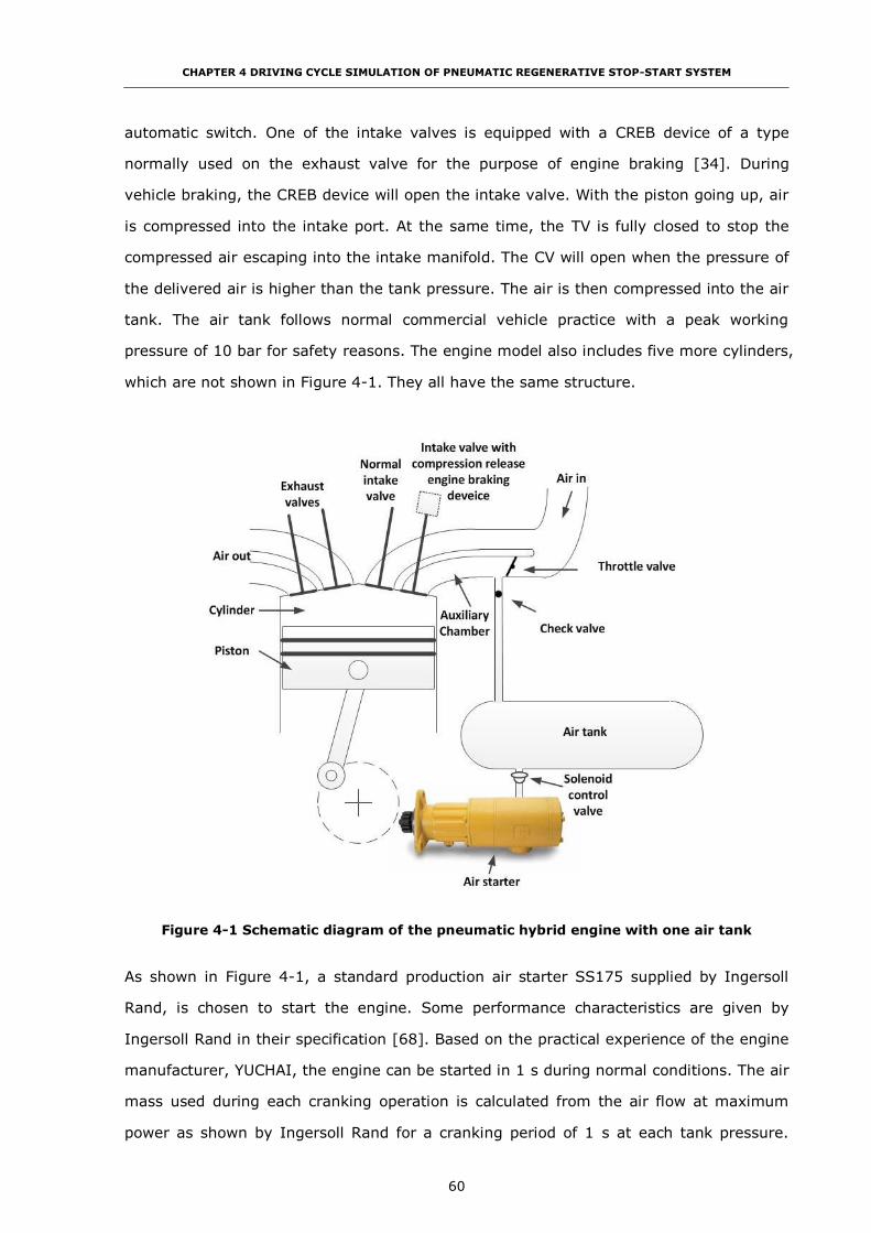
CHAPTER 4 DRIVING CYCLE SIMULATION OF PNEUMATIC REGENERATIVE STOP-START SYSTEM
60
automatic switch. One of the intake valves is equipped with a CREB device of a type
normally used on the exhaust valve for the purpose of engine braking [34]. During
vehicle braking, the CREB device will open the intake valve. With the piston going up, air
is compressed into the intake port. At the same time, the TV is fully closed to stop the
compressed air escaping into the intake manifold. The CV will open when the pressure of
the delivered air is higher than the tank pressure. The air is then compressed into the air
tank. The air tank follows normal commercial vehicle practice with a peak working
pressure of 10 bar for safety reasons. The engine model also includes five more cylinders,
which are not shown in Figure 4-1. They all have the same structure.
Figure 4-1 Schematic diagram of the pneumatic hybrid engine with one air tank
As shown in Figure 4-1, a standard production air starter SS175 supplied by Ingersoll
Rand, is chosen to start the engine. Some performance characteristics are given by
Ingersoll Rand in their specification [68]. Based on the practical experience of the engine
manufacturer, YUCHAI, the engine can be started in 1 s during normal conditions. The air
mass used during each cranking operation is calculated from the air flow at maximum
power as shown by Ingersoll Rand for a cranking period of 1 s at each tank pressure.

CHAPTER 4 DRIVING CYCLE SIMULATION OF PNEUMATIC REGENERATIVE STOP-START SYSTEM
61
From the specification, the air flow rates at different tank pressures are given [68]. Table
4-1 is the performance information about the SS175 air starter. From this table, the air
flow rates in different tank pressure are supplied. For example, when the tank pressure is
6.2 bar, the air flow would be 142 l/s to give a 1s cranking time, which means it
consumes 166.3 g air for 1 s operation in standard conditions for temperature and
pressure, 298 k and 1 bar. As a result, tank pressure will drop down to 5.2 bar after one
start-up operation.
Table 4-1 Air starter performance information [68]
Pressure
(Bar (PSI))
Breakaway
Torque
(Nm)
Speed
@ Max HP
(RPM)
Max Power
(kW (HP))
Flow
@ Max HP
(l/s)
6.2 (90) 42 2500 7 (10) 142
8.3 (120) 54 2700 10 (14) 189
10.3 (150) 70 2800 13 (18) 236
Also the specification gives the potential number of starts at various tank pressures and
for different tank sizes which shown in Table 4-2. In order to store sufficient compressed
air for the usage of the air starter, the size of the air tank is decided following the
recommendation of the air starter manufacturer [34]. The 151 l air tank is chosen to be
the energy storage device. It has a maximum working pressure of 10 bar and can
support 7 cranking attempts. The air starter also needs a minimum pressure of 5.2 bar
below which it will not operate reliably. The requirement placed on the control strategy is
therefore to keep the air tank pressure between 5.2 and 10 bar.
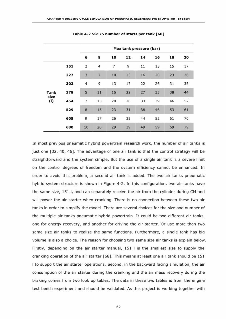
CHAPTER 4 DRIVING CYCLE SIMULATION OF PNEUMATIC REGENERATIVE STOP-START SYSTEM
62
Table 4-2 SS175 number of starts per tank [68]
Max tank pressure (bar)
6 8 10 12 14 16 18 20
Tank size
(l)
151 2 4 7 9 11 13 15 17
227 3 7 10 13 16 20 23 26
302 4 9 13 17 22 26 31 35
378 5 11 16 22 27 33 38 44
454 7 13 20 26 33 39 46 52
529 8 15 23 31 38 46 53 61
605 9 17 26 35 44 52 61 70
680 10 20 29 39 49 59 69 79
In most previous pneumatic hybrid powertrain research work, the number of air tanks is
just one [32, 40, 46]. The advantage of one air tank is that the control strategy will be
straightforward and the system simple. But the use of a single air tank is a severe limit
on the control degrees of freedom and the system efficiency cannot be enhanced. In
order to avoid this problem, a second air tank is added. The two air tanks pneumatic
hybrid system structure is shown in Figure 4-2. In this configuration, two air tanks have
the same size, 151 l, and can separately receive the air from the cylinder during CM and
will power the air starter when cranking. There is no connection between these two air
tanks in order to simplify the model. There are several choices for the size and number of
the multiple air tanks pneumatic hybrid powertrain. It could be two different air tanks,
one for energy recovery, and another for driving the air starter. Or use more than two
same size air tanks to realize the same functions. Furthermore, a single tank has big
volume is also a choice. The reason for choosing two same size air tanks is explain below.
Firstly, depending on the air starter manual, 151 l is the smallest size to supply the
cranking operation of the air starter [68]. This means at least one air tank should be 151
l to support the air starter operations. Second, in the backward facing simulation, the air
consumption of the air starter during the cranking and the air mass recovery during the
braking comes from two look up tables. The data in these two tables is from the engine
test bench experiment and should be validated. As this project is working together with

CHAPTER 4 DRIVING CYCLE SIMULATION OF PNEUMATIC REGENERATIVE STOP-START SYSTEM
63
Brunel University London, they chose 151 l air tank as the research objective and doing
the experimental test. In this stage, only the 151 l air tank has the confirmed data for
the two look up tables in the backward facing simulation. As a result, choosing two 151 l
air tank can guarantee the accuracy of the simulation. Also this research is meant to
investigate the potential ability of pneumatic hybrid powertrain in saving fuel for the bus
applications; it is not to optimize the pneumatic hybrid powertrain structure and
parameters. The result of this research supplies the fundamental understanding of the
pneumatic hybrid powertrain for the future research. The systems with more than two air
tanks are beyond the scope of this research. Therefore, two same size air tanks are
chosen for the two air tanks pneumatic hybrid powertrain. The remainder of the engine is
the same with one air tank pneumatic hybrid engine as shown in Figure 4-1.
Figure 4-2 Two air tanks pneumatic hybrid system structure
A pneumatic hybrid vehicle simulation model has been built using MATLAB/Simulink as
shown in Figure 4-3. This model is built with Quasi Steady State Toolbox (QSS-TB) with
some new blocks added. QSS-TB is a collection of MATLAB/Simulink blocks and the
appropriate parameter files that can be run in any MATLAB/Simulink environment [69].
QSS-TB permits a fast and simple estimation of the fuel consumption for many
powertrain systems. It can be used to calculate the vehicle fuel consumption, engine
speed and load required to achieve a given vehicle speed, rate of acceleration and
resistive loads such as rolling resistance, drag and frictional losses in the powertrain [70].
Vehicle and powertrain parameters, such as the mass of the vehicle, vehicle cross section

CHAPTER 4 DRIVING CYCLE SIMULATION OF PNEUMATIC REGENERATIVE STOP-START SYSTEM
64
area, wheel diameter, engine combustion maps, gear ratios, and driving cycle data, can
be defined in the different blocks of the model [69]. The QSS-TB is used in on-going
research projects and in the exercises to the lecture “Vehicle Propulsion Systems” by ETH
Zurich [71].
Figure 4-3 Pneumatic hybrid vehicle simulation model
Concerning this model, three different vehicle models are deployed. The models are
respectively “No Air Tank Model”, “One Air Tank Model” and “Two Air Tanks Model”. The
purpose of building the models with a common base specification is to compare results
directly. From Figure 4-3, it is evident that this is a backward vehicle driving cycle
simulation model. The driving cycle can be chosen (for example, Braunschweig cycle in
Figure 4-3) in the “Driving Cycle” block. The outputs of this block are the demand speed
v, demand acceleration dv, gear number and total distance of the driving cycle. Then, the
v and dv are the inputs of block “Vehicle”. In this block, the torque at the wheel (i.e.
resistances plus acceleration) is calculated and input to block “Manual Gear Box”. The
block “Manual Gear box” converts the wheel torque to a demanded net engine torque,
then input to three different blocks. In these three different blocks, based on different
pneumatic hybrid type, the torque combined with the speed of the engine will be

CHAPTER 4 DRIVING CYCLE SIMULATION OF PNEUMATIC REGENERATIVE STOP-START SYSTEM
65
calculated to obtain the fuel consumption. Within the block “Tank” those consumption
data are summarized and converted to a figure in l/100km. The equations for the models
mentioned before can be found in [69, 71].
Among the three models, the block structures are different, reflecting the different
vehicle architectures. The “No Air Tank Model” is based on the basic vehicle simulation
model in the QSS-TB. It gives the fuel consumption of a conventional diesel engine city
bus. The control strategy of this model is simple and is not developed further in the
report. The control strategies of “One Air Tank Model” and “Two Air Tanks Model” are
discussed in detail in the next section.
In order to achieve modularization of control system development and reduce the
possible cost of control system development, such as hardware design in the future,
Stateflow® in the MATLAB is used to complete the modelling and simulation. Stateflow is
an environment for modelling and simulating combinatorial and sequential decision logic
based on state machines and flow charts [72]. With Stateflow the logic for supervisory
control, task scheduling, and fault management applications can be designed. Stateflow
includes state machine animation and static and run-time checks for testing design
consistency and completeness before implementation making it easy to debug and
update the model [72]. The principal reason however for using Stateflow is that the
function of the pneumatic hybrid systems naturally consists of a number of states. Based
on state transition conditions, the model will transfer from one state to another. In
complex circumstances, secondary models manage a state transition within high level
states.
The relevant bus parameters are given in Table 4-3.
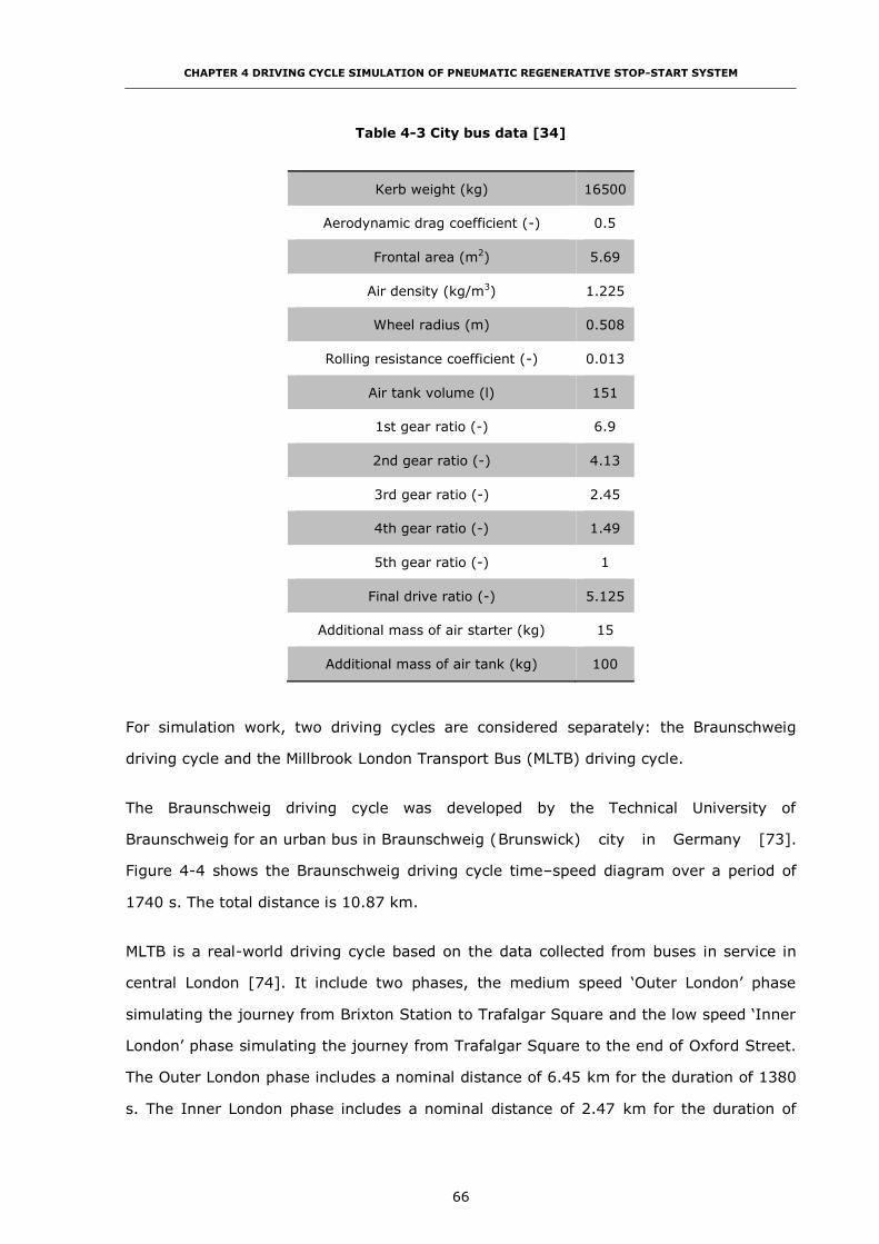
CHAPTER 4 DRIVING CYCLE SIMULATION OF PNEUMATIC REGENERATIVE STOP-START SYSTEM
66
Table 4-3 City bus data [34]
Kerb weight (kg) 16500
Aerodynamic drag coefficient (-) 0.5
Frontal area (m2) 5.69
Air density (kg/m3) 1.225
Wheel radius (m) 0.508
Rolling resistance coefficient (-) 0.013
Air tank volume (l) 151
1st gear ratio (-) 6.9
2nd gear ratio (-) 4.13
3rd gear ratio (-) 2.45
4th gear ratio (-) 1.49
5th gear ratio (-) 1
Final drive ratio (-) 5.125
Additional mass of air starter (kg) 15
Additional mass of air tank (kg) 100
For simulation work, two driving cycles are considered separately: the Braunschweig
driving cycle and the Millbrook London Transport Bus (MLTB) driving cycle.
The Braunschweig driving cycle was developed by the Technical University of
Braunschweig for an urban bus in Braunschweig ( Brunswick) city in Germany [73].
Figure 4-4 shows the Braunschweig driving cycle time–speed diagram over a period of
1740 s. The total distance is 10.87 km.
MLTB is a real-world driving cycle based on the data collected from buses in service in
central London [74]. It include two phases, the medium speed ‘Outer London’ phase
simulating the journey from Brixton Station to Trafalgar Square and the low speed ‘Inner
London’ phase simulating the journey from Trafalgar Square to the end of Oxford Street.
The Outer London phase includes a nominal distance of 6.45 km for the duration of 1380
s. The Inner London phase includes a nominal distance of 2.47 km for the duration of

CHAPTER 4 DRIVING CYCLE SIMULATION OF PNEUMATIC REGENERATIVE STOP-START SYSTEM
67
901 s. It covers in total 8.92 km for the duration of 2281 s. The time–speed diagram of
MLTB is shown in Figure 4-5.
Figure 4-4 Braunschweig driving cycle time–speed diagram
Figure 4-5 MLTB driving cycle time–speed diagram
Compared with the MLTB driving cycle, the Braunschweig driving cycle is characterized
with higher vehicle speeds and less stop–start operations over a slightly longer distance.
Table 4-4 shows the basic parameters of the Braunschweig driving cycle and the MLTB
driving cycle respectively.

CHAPTER 4 DRIVING CYCLE SIMULATION OF PNEUMATIC REGENERATIVE STOP-START SYSTEM
68
Table 4-4 Basic parameters of the MLTB driving cycle and Braunschweig driving cycle
Braunschweig driving cycle MLTB driving cycle
Time (s) 1740 2281
Distance (km) 10.87 8.92
Acceleration (%) 39.7 40.7
Deceleration (%) 30.8 30
Idle (%) 29.5 29.3
Number of stops (-) 30 52
4.3 Pneumatic Hybrid Powertrain Control Strategy
In the above pneumatic hybrid vehicle simulation models, the fuel consumption can be
reduced by (i) turning the engine off when the vehicle is stopped when the engine would
otherwise idle, or (ii) cut-off the fuel injection when implementing CM during vehicle
deceleration. Today, most diesel engines use fuel cut-off technology during the
deceleration to save the fuel. As a result, the only fuel that can be directly saved is that
used for idle. This means that when the vehicle is stopped and the engine would
otherwise be at idle speed, the engine is turned off. To realize this function, during the
deceleration, the pneumatic hybrid powertrain works in CM to compress air into the air
tank. When the vehicle implements the stop-start function, the compressed air is
supplied to the air starter to start the vehicle. The control strategy for the pneumatic
hybrid powertrain reflects the various functions of the system.
In the majority of prior work on pneumatic hybrid systems, the implementation employs
a single air tank, making the design and control solution relatively straightforward.
However, a second air tank provides an important degree of freedom to the control
system that leads to an enhancement of efficiency. The work reported in the following
sections includes the formulation and evaluation of a two tank model.
Much of the control strategy for respectively the one and two air tank models is common.
Firstly, once the engine braking torque which can be generated by the CM is less than the
braking torque, the CM is switched on. The air is compressed into the air tank. The
amount of air stored is then computed via the engine’s CM response map produced by
CHAPTER 4 DRIVING CYCLE SIMULATION OF PNEUMATIC REGENERATIVE STOP-START SYSTEM
69
the air hybrid engine simulation program from [34]. Both the engine speed and the tank
pressure are used as the input to two two-dimensional lookup tables to generate two
outputs: (a) the engine braking torque demand and (b) the amount of compressed air
storage, by using the interpolation and extrapolation method in every fixed-step
simulation time during the deceleration phase [34].
Because the air starter needs a minimum pressure in the air tank to start the engine, the
minimum pressure in the air tank must be 5.2 bar, no matter how many tanks. Activation
the stop–start mode is decided on the basis of the tank pressure.
The response map for the cranking mode takes into account the engine cranking speed
and compressed air mass consumption data from the air starter manual [75]. The final
air tank pressure is determined by the sum of compressed air production during CM and
consumption during the cranking.
This control strategy is suitable for the one air tank model. Figure 4-6 shows the control
block of one air tank model in the form of a Simulink model. The state diagram of control
strategy is shown in Figure 4-7 and its implementation in Stateflow is shown in Figure
4-8.

CHAPTER 4 DRIVING CYCLE SIMULATION OF PNEUMATIC REGENERATIVE STOP-START SYSTEM
70
Figure 4-6 One air tank simulation model control block
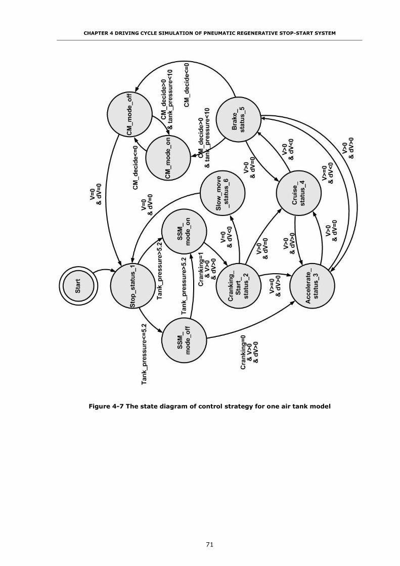
CHAPTER 4 DRIVING CYCLE SIMULATION OF PNEUMATIC REGENERATIVE STOP-START SYSTEM
71
Figure 4-7 The state diagram of control strategy for one air tank model
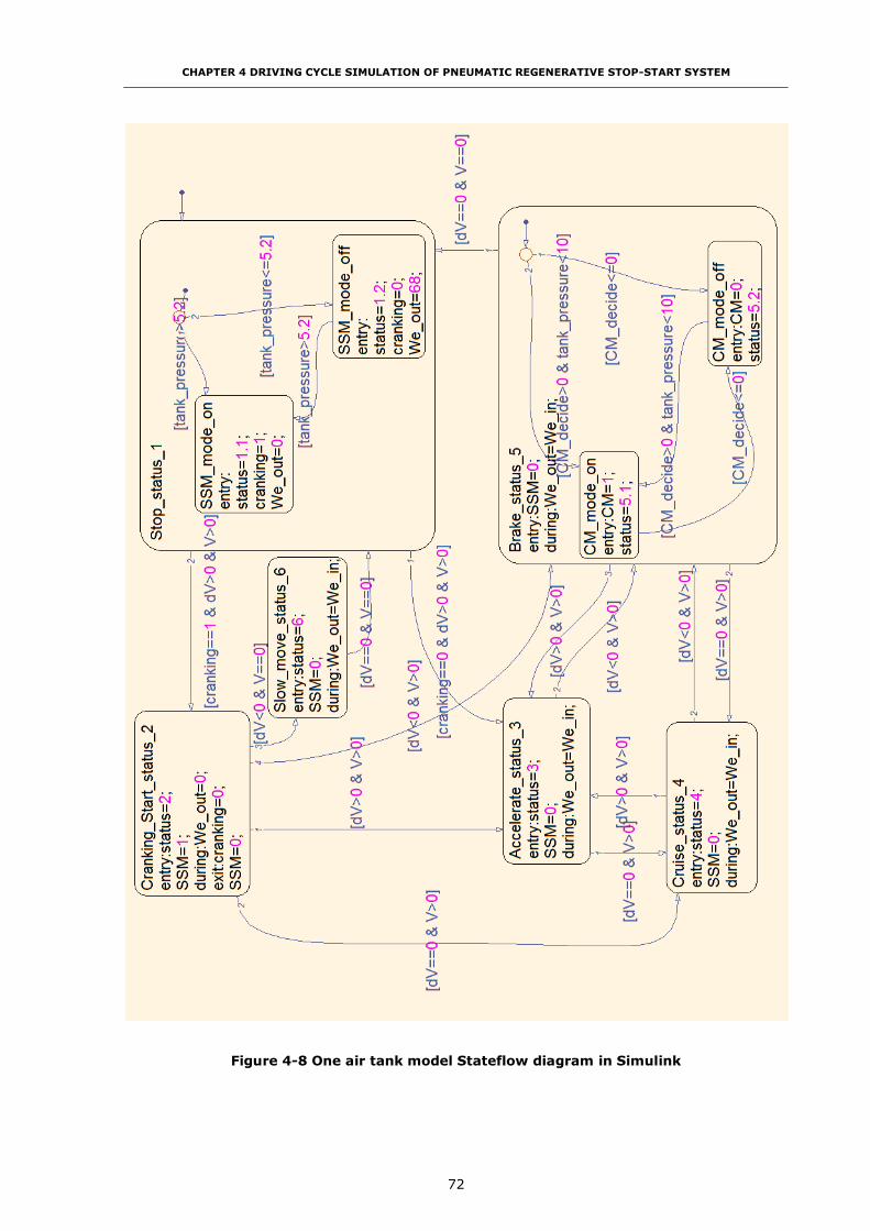
CHAPTER 4 DRIVING CYCLE SIMULATION OF PNEUMATIC REGENERATIVE STOP-START SYSTEM
72
Figure 4-8 One air tank model Stateflow diagram in Simulink

CHAPTER 4 DRIVING CYCLE SIMULATION OF PNEUMATIC REGENERATIVE STOP-START SYSTEM
73
Compared with the single air tank model, the two air tanks model is more complex.
Unlike the one air tank model, the air tank part of two air tanks model does not build
base on any existing engine structure. The model built here is to demonstrate the benefit
of using two air tanks in the pneumatic hybrid engine. In this model, two air tanks can
separately receive the air from the cylinder in the CM and drive the air starter when
cranking. There is no connection between these two air tanks. The reason to choose the
separate air tanks is because of the advantage that this structure can maintain at least
one air tank pressure as low as possible, and at same time to keep another air tank
pressure above the minimum air starter operation pressure 5.2 bar.
The key principle of the control strategy is to maximise the efficiency in CM. From the
previous research [34, 37], the air mass flow from cylinder to air tank in CM is
determined by the air tank pressure and engine speed. The lower air tank pressure can
recovery more air mass during the baking and supply more brake torque. Therefore, in
the two air tanks model, the control strategy is kept simple. When the vehicle enters CM,
a comparison is made of the pressure in the respective tanks and air tank with the lower
pressure will receive the air from the cylinder. When the vehicle starts, the lower
pressure air tank is allocated to supply the air starter, as long as it is above the minimum
pressure of 5.2 bar. So in the two air tanks model, the pressures need to be monitored
and compared. The control strategy compares the two pressures and decides which tank
is to receive the air during CM and which one supplies air to start the engine. The control
block, state diagram and Stateflow diagram are shown in Figure 4-9, Figure 4-10 and
Figure 4-11. Since this research is to investigate how to manage the pneumatic energy,
it only considers the aspects related to the energy. Other aspects such as how to actual
implement the system, how to engage the clutch will not be discussed here.

CHAPTER 4 DRIVING CYCLE SIMULATION OF PNEUMATIC REGENERATIVE STOP-START SYSTEM
74
Figure 4-9 Two air tanks model control block

CHAPTER 4 DRIVING CYCLE SIMULATION OF PNEUMATIC REGENERATIVE STOP-START SYSTEM
75
Figure 4-10 The state diagram of control strategy for two air tanks model
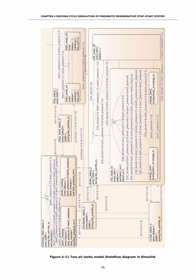
CHAPTER 4 DRIVING CYCLE SIMULATION OF PNEUMATIC REGENERATIVE STOP-START SYSTEM
76
Figure 4-11 Two air tanks model Stateflow diagram in Simulink
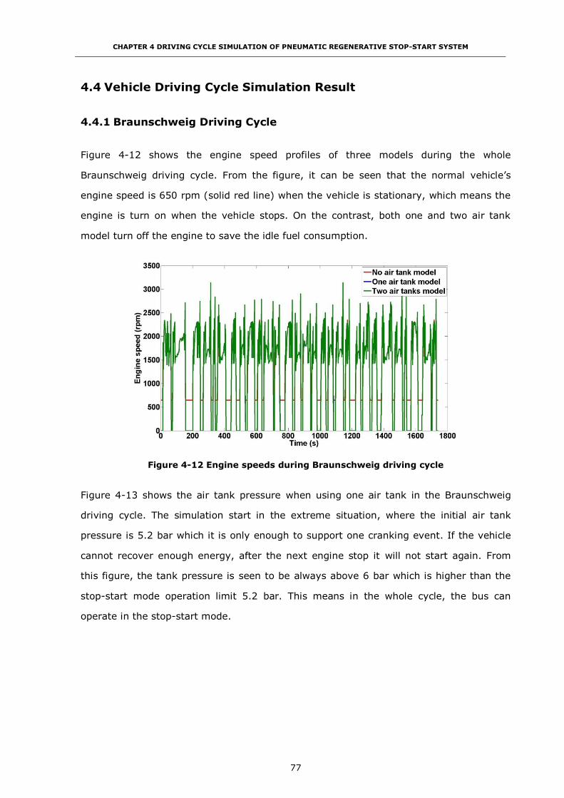
CHAPTER 4 DRIVING CYCLE SIMULATION OF PNEUMATIC REGENERATIVE STOP-START SYSTEM
77
4.4 Vehicle Driving Cycle Simulation Result
4.4.1 Braunschweig Driving Cycle
Figure 4-12 shows the engine speed profiles of three models during the whole
Braunschweig driving cycle. From the figure, it can be seen that the normal vehicle’s
engine speed is 650 rpm (solid red line) when the vehicle is stationary, which means the
engine is turn on when the vehicle stops. On the contrast, both one and two air tank
model turn off the engine to save the idle fuel consumption.
Figure 4-12 Engine speeds during Braunschweig driving cycle
Figure 4-13 shows the air tank pressure when using one air tank in the Braunschweig
driving cycle. The simulation start in the extreme situation, where the initial air tank
pressure is 5.2 bar which it is only enough to support one cranking event. If the vehicle
cannot recover enough energy, after the next engine stop it will not start again. From
this figure, the tank pressure is seen to be always above 6 bar which is higher than the
stop-start mode operation limit 5.2 bar. This means in the whole cycle, the bus can
operate in the stop-start mode.
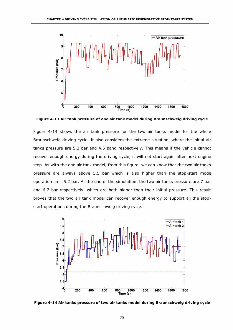
CHAPTER 4 DRIVING CYCLE SIMULATION OF PNEUMATIC REGENERATIVE STOP-START SYSTEM
78
Figure 4-13 Air tank pressure of one air tank model during Braunschweig driving cycle
Figure 4-14 shows the air tank pressure for the two air tanks model for the whole
Braunschweig driving cycle. It also considers the extreme situation, where the initial air
tanks pressure are 5.2 bar and 4.5 band respectively. This means if the vehicle cannot
recover enough energy during the driving cycle, it will not start again after next engine
stop. As with the one air tank model, from this figure, we can know that the two air tanks
pressure are always above 5.5 bar which is also higher than the stop-start mode
operation limit 5.2 bar. At the end of the simulation, the two air tanks pressure are 7 bar
and 6.7 bar respectively, which are both higher than their initial pressure. This result
proves that the two air tank model can recover enough energy to support all the stop-
start operations during the Braunschweig driving cycle.
Figure 4-14 Air tanks pressure of two air tanks model during Braunschweig driving cycle
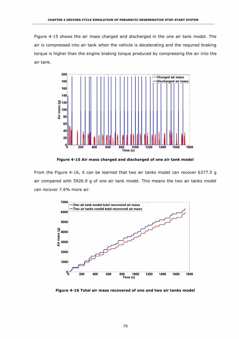
CHAPTER 4 DRIVING CYCLE SIMULATION OF PNEUMATIC REGENERATIVE STOP-START SYSTEM
79
Figure 4-15 shows the air mass charged and discharged in the one air tank model. The
air is compressed into air tank when the vehicle is decelerating and the required braking
torque is higher than the engine braking torque produced by compressing the air into the
air tank.
Figure 4-15 Air mass charged and discharged of one air tank model
From the Figure 4-16, it can be learned that two air tanks model can recover 6377.5 g
air compared with 5926.9 g of one air tank model. This means the two air tanks model
can recover 7.6% more air.
Figure 4-16 Total air mass recovered of one and two air tanks model
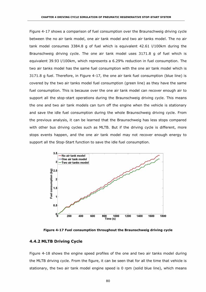
CHAPTER 4 DRIVING CYCLE SIMULATION OF PNEUMATIC REGENERATIVE STOP-START SYSTEM
80
Figure 4-17 shows a comparison of fuel consumption over the Braunschweig driving cycle
between the no air tank model, one air tank model and two air tanks model. The no air
tank model consumes 3384.8 g of fuel which is equivalent 42.61 l/100km during the
Braunschweig driving cycle. The one air tank model uses 3171.8 g of fuel which is
equivalent 39.93 l/100km, which represents a 6.29% reduction in fuel consumption. The
two air tanks model has the same fuel consumption with the one air tank model which is
3171.8 g fuel. Therefore, in Figure 4-17, the one air tank fuel consumption (blue line) is
covered by the two air tanks model fuel consumption (green line) as they have the same
fuel consumption. This is because over the one air tank model can recover enough air to
support all the stop-start operations during the Braunschweig driving cycle. This means
the one and two air tank models can turn off the engine when the vehicle is stationary
and save the idle fuel consumption during the whole Braunschweig driving cycle. From
the previous analysis, it can be learned that the Braunschweig has less stops compared
with other bus driving cycles such as MLTB. But if the driving cycle is different, more
stops events happen, and the one air tank model may not recover enough energy to
support all the Stop-Start function to save the idle fuel consumption.
Figure 4-17 Fuel consumption throughout the Braunschweig driving cycle
4.4.2 MLTB Driving Cycle
Figure 4-18 shows the engine speed profiles of the one and two air tanks model during
the MLTB driving cycle. From the figure, it can be seen that for all the time that vehicle is
stationary, the two air tank model engine speed is 0 rpm (solid blue line), which means

CHAPTER 4 DRIVING CYCLE SIMULATION OF PNEUMATIC REGENERATIVE STOP-START SYSTEM
81
the engine is turned off when the vehicle stops. On the contrast, the one air tank model
turn on the engine for 4 times, which shows in the Figure 4-18 is engine speed at 650
rpm (solid red line). It means the one air tank model eliminate more than 90% (48 of 52)
of the idling time. The reason that cannot eliminate 100% is because during the MLTB
driving cycle, one air tank model cannot recover enough air to support all the stop-start
operations which means the air tank pressure will drop below 5.2 bar before the vehicle
stops sometimes. As a result, the engine cannot be switched off to avoid the situation
that there is no enough air to support one cranking event.
Figure 4-18 Engine speeds during MLTB driving cycle
Figure 4-19 shows the air tank pressure of one air tank model. Similar to the
Braunschweig driving cycle simulation, this simulation start in the extreme situation,
where the initial air tank pressure is 5.2 bar. At the end of the simulation, the air tank
pressure is 5.5 bar which is still higher than its initial pressure. In this figure, the
pressure of air tank will drop below the working limit, 5.2 bar. This is because, in the
MLTB driving cycle, the interval between two stops is too short which cause the vehicle
cannot recover enough energy. For example, after 1500 s in the MLTB, there are four
continuous stops which are shown in Figure 4-19 is four pressure drops of the air tank. It
means the engine is turned off four times and implemented four cranking events. The
result is that the tank pressure drops from 8.2 bar to 4.5 bar. In other words, it means
the vehicle needs more air to drive the air starter compared with the opportunity to
recover air. But comparing with the air tanks pressure of two air tanks model in Figure
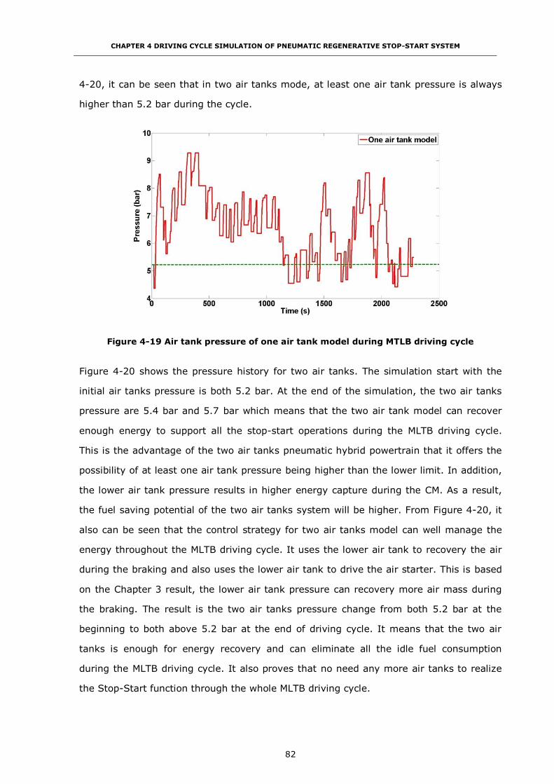
CHAPTER 4 DRIVING CYCLE SIMULATION OF PNEUMATIC REGENERATIVE STOP-START SYSTEM
82
4-20, it can be seen that in two air tanks mode, at least one air tank pressure is always
higher than 5.2 bar during the cycle.
Figure 4-19 Air tank pressure of one air tank model during MTLB driving cycle
Figure 4-20 shows the pressure history for two air tanks. The simulation start with the
initial air tanks pressure is both 5.2 bar. At the end of the simulation, the two air tanks
pressure are 5.4 bar and 5.7 bar which means that the two air tank model can recover
enough energy to support all the stop-start operations during the MLTB driving cycle.
This is the advantage of the two air tanks pneumatic hybrid powertrain that it offers the
possibility of at least one air tank pressure being higher than the lower limit. In addition,
the lower air tank pressure results in higher energy capture during the CM. As a result,
the fuel saving potential of the two air tanks system will be higher. From Figure 4-20, it
also can be seen that the control strategy for two air tanks model can well manage the
energy throughout the MLTB driving cycle. It uses the lower air tank to recovery the air
during the braking and also uses the lower air tank to drive the air starter. This is based
on the Chapter 3 result, the lower air tank pressure can recovery more air mass during
the braking. The result is the two air tanks pressure change from both 5.2 bar at the
beginning to both above 5.2 bar at the end of driving cycle. It means that the two air
tanks is enough for energy recovery and can eliminate all the idle fuel consumption
during the MLTB driving cycle. It also proves that no need any more air tanks to realize
the Stop-Start function through the whole MLTB driving cycle.

CHAPTER 4 DRIVING CYCLE SIMULATION OF PNEUMATIC REGENERATIVE STOP-START SYSTEM
83
Figure 4-20 Air tanks pressure of two air tanks model throughout MLTB driving cycle
Figure 4-21 shows a comparison of fuel consumption over the MLTB driving cycle
between the no air tank model, one air tank model and two air tanks model. The no air
tank model consumes 3743.2 g of fuel which is equivalent 57.14 l/100km during the
MLTB driving cycle. The one air tank model uses 3501.7 g of fuel which is equivalent
53.45 l/100km, which represents a 6.45% reduction in fuel consumption. The two air
tanks model uses 3477.6 g of fuel which is equivalent 53.09 l/100km, which represents a
7.1% reduction in fuel consumption compared with no air tank model. The two air tanks
model also reduces the fuel consumption 0.7% compared to the one air tank model. This
is because the two air tanks model can recover enough air to support all the stop-start
operations during the MLTB driving cycle, while the one air tank model only can support
most of the stop-start operations. The result proves that by turning off the engine when
the vehicle is stationary to save the idle fuel consumption, a 7.1% reduction in fuel
consumption can be achieved in the MLTB driving cycle. In Chapter 2, a fuel consumption
result comparison is given out. From the result, it can be seen that if only considering the
stop-start operations, the fuel consumption improvement is in the range of 6% to 20%
depending on the vehicles and test cycles used. This means the fuel consumption saving
of 7.1% here is similar to the result reported within the literatures.
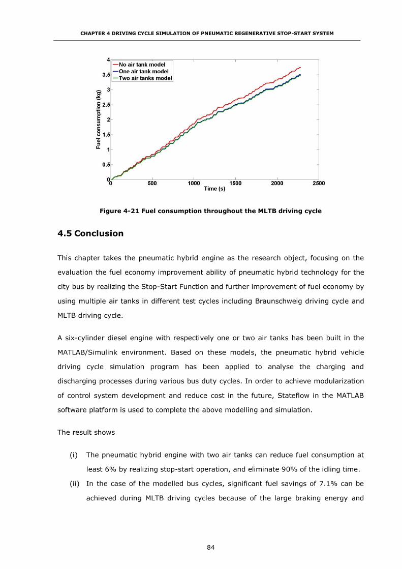
CHAPTER 4 DRIVING CYCLE SIMULATION OF PNEUMATIC REGENERATIVE STOP-START SYSTEM
84
Figure 4-21 Fuel consumption throughout the MLTB driving cycle
4.5 Conclusion
This chapter takes the pneumatic hybrid engine as the research object, focusing on the
evaluation the fuel economy improvement ability of pneumatic hybrid technology for the
city bus by realizing the Stop-Start Function and further improvement of fuel economy by
using multiple air tanks in different test cycles including Braunschweig driving cycle and
MLTB driving cycle.
A six-cylinder diesel engine with respectively one or two air tanks has been built in the
MATLAB/Simulink environment. Based on these models, the pneumatic hybrid vehicle
driving cycle simulation program has been applied to analyse the charging and
discharging processes during various bus duty cycles. In order to achieve modularization
of control system development and reduce cost in the future, Stateflow in the MATLAB
software platform is used to complete the above modelling and simulation.
The result shows
(i) The pneumatic hybrid engine with two air tanks can reduce fuel consumption at
least 6% by realizing stop-start operation, and eliminate 90% of the idling time.
(ii) In the case of the modelled bus cycles, significant fuel savings of 7.1% can be
achieved during MLTB driving cycles because of the large braking energy and
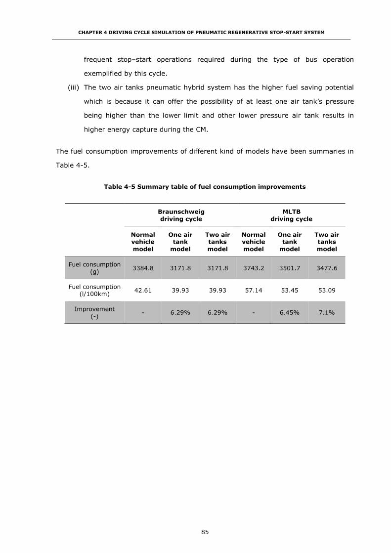
CHAPTER 4 DRIVING CYCLE SIMULATION OF PNEUMATIC REGENERATIVE STOP-START SYSTEM
85
frequent stop–start operations required during the type of bus operation
exemplified by this cycle.
(iii) The two air tanks pneumatic hybrid system has the higher fuel saving potential
which is because it can offer the possibility of at least one air tank’s pressure
being higher than the lower limit and other lower pressure air tank results in
higher energy capture during the CM.
The fuel consumption improvements of different kind of models have been summaries in
Table 4-5.
Table 4-5 Summary table of fuel consumption improvements
Braunschweig
driving cycle
MLTB
driving cycle
Normal vehicle
model
One air tank
model
Two air tanks
model
Normal vehicle
model
One air tank
model
Two air tanks
model
Fuel consumption
(g) 3384.8 3171.8 3171.8 3743.2 3501.7 3477.6
Fuel consumption (l/100km)
42.61 39.93 39.93 57.14 53.45 53.09
Improvement
(-) - 6.29% 6.29% - 6.45% 7.1%

CHAPTER 5 ANALYSIS OF THE PNEUMATIC REGENERATIVE BRAKING SYSTEM
86
CHAPTER 5
ANALYSIS OF THE PNEUMATIC REGENERATIVE BRAKING
SYSTEM
5.1 Introduction
Recovering braking energy and reusing it can significantly improve the fuel economy of a
vehicle which is subject to frequent braking events such as a city bus. As one way to
achieve this goal, the pneumatic hybrid technology converts kinetic energy to pneumatic
energy by compressing air into the tanks during braking, and then reuses the
compressed air to power an air starter to realize a regenerative Stop-Start function. This
has already been investigated in Chapter 4. The pneumatic hybrid city bus uses the
driven rear axle to achieve the regenerative braking function. Because the majority of
hybrid and electric and battery electric vehicle employ front wheel drive, this aspect of
the architecture represents a significant difference with light duty vehicles which has
consequences for the choice of braking strategy. This chapter discusses the research into
the blending of pneumatic regenerative braking and mechanical frictional braking at the
rear axle. The aim of the braking function is to recover as much energy as possible and
at the same time distribute the total braking effort between the front and rear axles to
achieve stable braking performance.
This chapter firstly presents an analysis of vehicle behaviour through different bus driving
cycles and during braking events, and then compares two configurations of the hybrid
braking system. The respective configurations, a parallel hybrid brake system and a fully
controllable hybrid brake system, are compared and the control strategy presented and
discussed. The comparison shows the fully controllable hybrid braking system has a
distinct advantage and is chosen to realize the regenerative braking function.
A pneumatic hybrid braking optimisation simulation model has been built in the
MATLAB/Simulink environment to facilitate an investigation of an optimum air tank
pressure for energy recovery. Similar to the models in Chapter 4, this model is also built
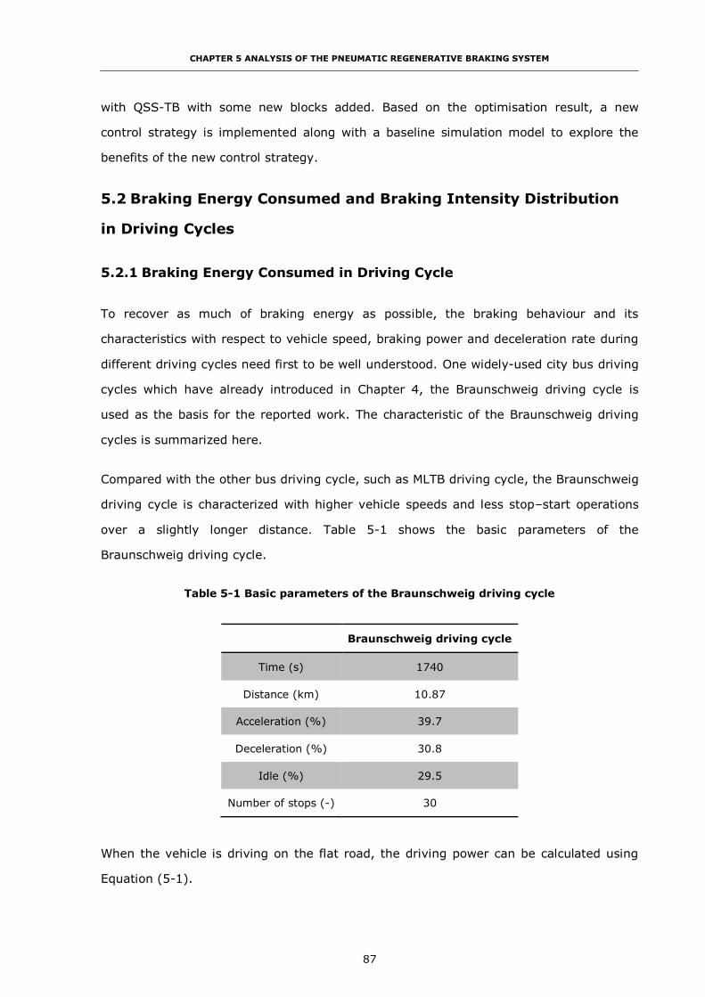
CHAPTER 5 ANALYSIS OF THE PNEUMATIC REGENERATIVE BRAKING SYSTEM
87
with QSS-TB with some new blocks added. Based on the optimisation result, a new
control strategy is implemented along with a baseline simulation model to explore the
benefits of the new control strategy.
5.2 Braking Energy Consumed and Braking Intensity Distribution
in Driving Cycles
5.2.1 Braking Energy Consumed in Driving Cycle
To recover as much of braking energy as possible, the braking behaviour and its
characteristics with respect to vehicle speed, braking power and deceleration rate during
different driving cycles need first to be well understood. One widely-used city bus driving
cycles which have already introduced in Chapter 4, the Braunschweig driving cycle is
used as the basis for the reported work. The characteristic of the Braunschweig driving
cycles is summarized here.
Compared with the other bus driving cycle, such as MLTB driving cycle, the Braunschweig
driving cycle is characterized with higher vehicle speeds and less stop–start operations
over a slightly longer distance. Table 5-1 shows the basic parameters of the
Braunschweig driving cycle.
Table 5-1 Basic parameters of the Braunschweig driving cycle
Braunschweig driving cycle
Time (s) 1740
Distance (km) 10.87
Acceleration (%) 39.7
Deceleration (%) 30.8
Idle (%) 29.5
Number of stops (-) 30
When the vehicle is driving on the flat road, the driving power can be calculated using
Equation (5-1).

CHAPTER 5 ANALYSIS OF THE PNEUMATIC REGENERATIVE BRAKING SYSTEM
88
𝑃𝑑 =𝑣
1000(𝑀𝑔𝑓𝑟 +
1
2𝜌𝑎𝐶𝐷𝐴𝑣2 + 𝑀𝛿
𝑑𝑣
𝑑𝑡) (5-1) [6]
where Pd - driving power,
M - vehicle mass,
g - gravitational acceleration,
fr - tire rolling resistance coefficient,
ρa - air mass density,
CD - aerodynamic drag coefficient,
A - frontal area of the vehicle,
v - vehicle speed,
δ - rotational inertia factor,
dv/dt - vehicle acceleration or deceleration (m/s2).
If Pd>0, the powertrain of the vehicle exports power to the wheels to drive the vehicle
forward. Otherwise, Pd<0, the braking and kinetic energy of the vehicle is dissipated by
the braking system. This is the energy that should be recovered and reused to reduce the
fuel consumption.
The parameters of the city bus used in the reported work are listed in Table 5-2.
Table 5-2 City bus data
Vehicle Total weight (kg) 16500
Aerodynamic drag coefficient (-) 0.5
Frontal area (m2) 5.69
Wheel radius (m) 0.508
Rolling resistance coefficient (-) 0.013
Wheel base (m) 6.1
Distance from gravity centre to front wheel centre (m) 4
Gravity centre height (m) 1
The traction and braking energy dissipated during the Braunschweig driving cycle are
calculated and shown in Figure 5-1 which indicates that in the urban area the bus’s
braking power can reach to 80% of the total traction power.

CHAPTER 5 ANALYSIS OF THE PNEUMATIC REGENERATIVE BRAKING SYSTEM
89
Figure 5-1 Traction and braking power dissipation in Braunschweig driving cycle
5.2.2 Braking Intensity Distribution in Driving Cycles
Another important consideration is the braking intensity in different city bus driving
cycles. Understanding this is very helpful to the proper design of an optimal control
strategy and the system sizing. Figure 5-2 and Figure 5-3 show the deceleration
distribution during the Braunschweig driving cycle and the MLTB driving cycle. It can be
seen in these figures that, during the Braunschweig driving cycle and the MLTB driving
cycle respectively, the braking of the city bus is very gentle with most of the deceleration
rate below 0.2 g, compared with the passenger car whose mean fully developed
deceleration is 0.51 g (equal to 5.0 m/s2) [67]. Therefore, this work only considers
braking behaviour corresponding to decelerations up to 0.4 g.
Figure 5-2 Deceleration distribution during Braunschweig driving cycle
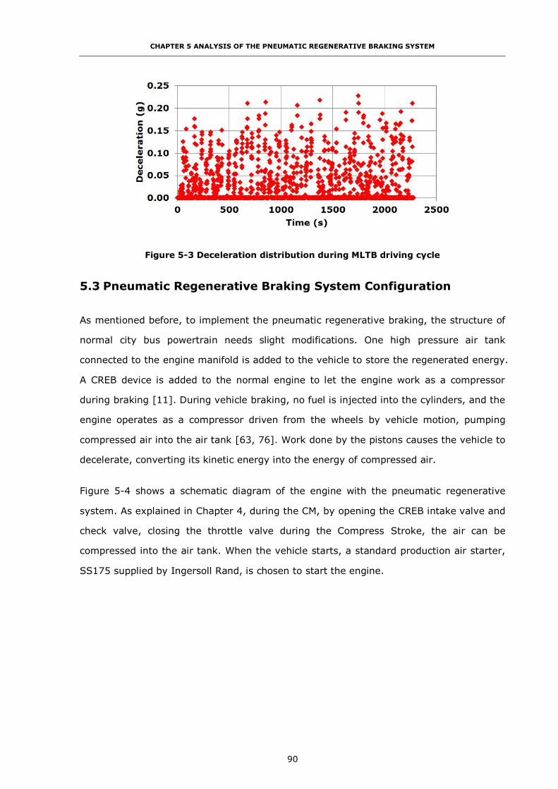
CHAPTER 5 ANALYSIS OF THE PNEUMATIC REGENERATIVE BRAKING SYSTEM
90
Figure 5-3 Deceleration distribution during MLTB driving cycle
5.3 Pneumatic Regenerative Braking System Configuration
As mentioned before, to implement the pneumatic regenerative braking, the structure of
normal city bus powertrain needs slight modifications. One high pressure air tank
connected to the engine manifold is added to the vehicle to store the regenerated energy.
A CREB device is added to the normal engine to let the engine work as a compressor
during braking [11]. During vehicle braking, no fuel is injected into the cylinders, and the
engine operates as a compressor driven from the wheels by vehicle motion, pumping
compressed air into the air tank [63, 76]. Work done by the pistons causes the vehicle to
decelerate, converting its kinetic energy into the energy of compressed air.
Figure 5-4 shows a schematic diagram of the engine with the pneumatic regenerative
system. As explained in Chapter 4, during the CM, by opening the CREB intake valve and
check valve, closing the throttle valve during the Compress Stroke, the air can be
compressed into the air tank. When the vehicle starts, a standard production air starter,
SS175 supplied by Ingersoll Rand, is chosen to start the engine.

CHAPTER 5 ANALYSIS OF THE PNEUMATIC REGENERATIVE BRAKING SYSTEM
91
Figure 5-4 Schematic diagram of the engine with pneumatic regenerative system
5.4 Pneumatic Regenerative Braking Control Strategy
Like the regenerative braking system in vehicles with electric propulsion, there are also
two configurations of hybrid braking system in the pneumatic hybrid city bus,
respectively
(i) the parallel hybrid brake system,
(ii) the fully controllable hybrid brake system.
(i) has a simple structure and control and retains all the major components of the
conventional braking system; (ii) can fully control the braking force for each individual
wheel, thus greatly enhancing the vehicle’s braking performance on all types of roads [6].
In the pneumatic hybrid city bus, during braking, the engine becomes a compressor and
directly applies its braking torque to the rear axle. The research question is then - how to
distribute and blend this torque with the vehicle mechanical braking torque on the rear
axle and front axle? This question will be answered in the following sections.

CHAPTER 5 ANALYSIS OF THE PNEUMATIC REGENERATIVE BRAKING SYSTEM
92
5.4.1 Parallel Hybrid Pneumatic City Bus Braking System Control
Strategy
The parallel hybrid braking system retains all the major components of the conventional
mechanical brakes and adds the pneumatic braking torque on the rear axle. The
pneumatic braking torque will be created by the engine and managed by the controller.
The controller will calculate the ratio of mechanical braking force and pneumatic braking
force based on vehicle speed, deceleration and the pressure of the air tank.
Figure 5-5 shows the braking force distribution strategy which is the key point of the
control strategy of this kind of system. In the parallel hybrid braking system, the
mechanical braking system still has a fixed ratio of braking force distribution on the front
and rear axles represented by the β-line [77].
Figure 5-5 Control strategy for the parallel hybrid braking system
When the vehicle is braking, the loads of the front and rear wheels vary with the
deceleration of the vehicle. In order to keep the vehicle stable while braking, the braking

CHAPTER 5 ANALYSIS OF THE PNEUMATIC REGENERATIVE BRAKING SYSTEM
93
force acting on the front and rear wheels should be limited in a reasonable range [78].
The normal load on the front axle Wf can be determined as
𝑊𝑓 =𝑚𝑔
𝐿(𝑏 + ℎ𝑔
𝑗
𝑔) (5-2) [78]
Similarly, the normal load acting on the rear axle Wr can be expressed as
𝑊𝑟 =𝑚𝑔
𝐿(𝑎 − ℎ𝑔
𝑗
𝑔) (5-3) [78]
where 𝑗 – deceleration rate of the vehicle,
hg – gravity centre height of the vehicle,
a – distance from gravity centre to front wheel centre,
b – distance from the gravity centre to front wheel centre,
𝑔 – gravitational acceleration,
L – wheel base.
Braking force acting on the front and rear wheels are required to be proportional to their
corresponding normal load. Such a distribution of the braking forces on front and rear
wheels can be obtain the maximum braking stability of the vehicle [79]. Therefore, the
relationship of the braking force on front and rear wheels, associating with the
deceleration of the vehicle, can be expressed as:
𝐹𝑓
𝐹𝑟=
𝑎+ℎ𝑔𝑗
𝑔
𝑏−ℎ𝑔𝑗
𝑔
(5-4) [78]
The summation of the braking forces of the front and rear wheels (the total barking force
of the vehicle) is related to the vehicle deceleration by
𝐹𝑓 + 𝐹𝑟 = 𝑚𝑔𝑗 (5-5) [78]
Substituting Equation (5-5) into (5-4) gives out the ideal distribution of the braking
forces on the front and rear wheels as:
𝐹𝑟 =1
2[
𝐺
ℎ𝑔√𝑏2 +
4ℎ𝑔𝐿
𝐺𝐹𝑓 − (
𝐺𝑏
ℎ𝑔+ 2𝐹𝑓)] (5-6) [6]
where 𝐹𝑟 – total braking force on the rear wheels,
𝐺 – gravity of the vehicle,

CHAPTER 5 ANALYSIS OF THE PNEUMATIC REGENERATIVE BRAKING SYSTEM
94
ℎ𝑔 – gravity centre height,
𝑏 – distance from gravity centre to rear wheel centre,
𝐿 – wheel base,
𝐹𝑓 – total braking force on the front wheels.
The I-Curve shown in Figure 5-5 and Figure 5-7 can be calculated by this equation. The
I-Curve shows the ideal braking force distribution of the vehicle [80]. This ideal
distribution curve gives the maximum braking force that makes the front and rear wheels
lock simultaneously for each friction coefficient. When the braking force is distributed to
the front and rear wheels on the I-Curve, safe braking is assured.
If most of the braking force is applied to the rear wheel and a very small force to the
front wheels, there will be a reduced utilization of road adhesion. To avoid this situation,
brake design regulations have been developed. Typical is The Economic Commission of
Europe (ECE) brake regulation [81]. The ECE regulation indicates the minimum braking
force on the rear wheels, which can be calculated by Equation (5-7), and also shown in
Figure 5-5 and Figure 5-7 The physical meaning of this equation is that when the front
wheels are locked, the rear braking force must be large enough to make the vehicle yield
a deceleration rate not smaller than the value dictated by Equation (5-7) [80].
𝑗
𝑔≥ 0.1 + 0.85(𝜇 − 0.2) (5-7) [80]
where 𝑗 – deceleration rate of the vehicle,
𝜇 – adhesion coefficient,
𝑔 – gravitational acceleration.
The total braking force on the rear axle consists of mechanical braking, Fbr-mech, and
pneumatic braking, Fbr-regen, as shown in the Figure 5-5. In order to recover maximum
braking energy, the pneumatic hybrid braking system should employ the pneumatic
braking force on the rear axle as much as possible during the whole vehicle operation
range. Based on the investigation mentioned before, during the MLTB driving cycle and
Braunschweig driving cycle, the braking is very gentle with most of the deceleration rate
below 0.2 g, while the maximum deceleration rate of these two driving cycle is 0.4 g. For
this reason when the deceleration is less than 0.4 g, both mechanical and pneumatic
braking systems share the total rear axle braking force. When the required deceleration

CHAPTER 5 ANALYSIS OF THE PNEUMATIC REGENERATIVE BRAKING SYSTEM
95
is greater than 0.4 g, the pneumatic braking force is reduced to zero and only mechanical
braking works on the rear axle to get stable and sufficient braking force. Although the
system can maintain the pneumatic braking force as high as possible, and simply
supplement with the friction braking system when the deceleration is greater than 0.4 g.
It may cause an unsafe situation when the driver brakes urgently. The driver would
release to clutch to stop the vehicle during the braking period. The releasing the clutch
would stop the braking force from pneumatic braking system and this may cause the
braking force dropping sharply which made the vehicle braking behaviour unstable. As a
result, the ideal control strategy for a parallel braking system is when the deceleration is
less than 0.4 g and the braking force distribution follows the I-curve, otherwise, it follows
the β-line. However, this strategy cannot be realised in a practical implementation of the
parallel hybrid braking system, the reason will be explained in the following paragraphs.
For example, in Figure 5-5, if the vehicle’s deceleration rate is 0.12 g, the red line, the
maximum braking force ratio that makes the front and rear wheels lock simultaneously is
point A which is on the I-Curve. The mechanical braking system can supply a fixed ratio
braking force on the front and rear axles that follow the β line, point B in Figure 5-5.
From A to B is the range of force that the pneumatic braking system needs to supply. If it
is an electric regenerative braking system, the controller can control the electric motor to
create the requested braking force if it does not exceed the motor’s working range. But
in the pneumatic braking system, during braking, the pneumatic braking system may not
be able to supply the exact braking force Fbr-regen, which is shown in Figure 5-5 as A to B
at every moment. This is because the pneumatic hybrid braking system’s characteristic
that the braking torque created by the pneumatic braking system is related to the air
tank pressure. During braking, the engine operates as a compressor driven from the
wheels by vehicle motion and pumping compressed air into the air tank. At the same
time, there is no fuel injected into the cylinders. Work performed by the pistons slows
down the vehicle and converts its kinetic energy into energy of compressed air [4]. The
result from Chapter 3, as shown in Figure 3-15, has already supplied the relationship
between the brake torque and air tank pressure, which is the lower air tank pressure can
create more brake torque at the same engine speed. It means the small air tank
pressure is beneficial to improve the engine braking performance based on the engine
using in this research.

CHAPTER 5 ANALYSIS OF THE PNEUMATIC REGENERATIVE BRAKING SYSTEM
96
Also in Schechter’s research [63], Figure 5-6 clearly indicated that the engine IMEP is
related to the air tank pressure which the lower air tank pressure may not create higher
IMEP. It can be seen when the air tank pressure higher than 0.8 MPa (equal to 8 bar),
the IMEP decreases when the air tank pressure increases, which accord with the Chapter
3 result, the lower air tank pressure can create more brake torque. But when the air tank
pressure is lower than 0.8 MPa, the result is different with the result from Chapter 3. This
is because Schechter used a different engine structure in his research. Also in the same
paper, an Equation (5-8) was derived to compute the peak value of IMEP as a function of
air-tank pressure during the braking process [63].
Figure 5-6 IMEP in a Type 1 compression-braking cycle [63]
𝐼𝑀𝐸𝑃 = 2(𝜌𝑐𝑣𝑇2 + 𝑝2)(𝑟𝑘−1 − 1)(𝑅 − 𝑟)/(𝑅 − 1) (5-8) [63]
where 𝜌 – air density,
𝑐𝑣 – specific heat at constant volume,
𝑇2 – air temperature,
𝑝2 – air pressure,
𝑟 – compression ratio from point 2 to point 3,
𝑘 – ratio of specific heats,
𝑅 – geometric compression ratio.
Based on the Equation (5-8), the braking force Fbr-regen created by the engine during the
braking can be calculated from engine’s IMEP. Unlike the electric regenerative braking
technology, this braking force, Fbr-regen is based on the air tank pressure at each instant.
That means the pneumatic braking system may not be able to supply the exact braking

CHAPTER 5 ANALYSIS OF THE PNEUMATIC REGENERATIVE BRAKING SYSTEM
97
force that the controller requires. As a result, the vehicle may not be able to follow the I-
curve. This represents a fundamental difficulty in the application of this method. Instead,
a fully controllable system that is able to follow the I-Curve is reviewed in the following
sections of the paper.
5.4.2 Fully Controllable Pneumatic Hybrid City Bus Braking System
Control Strategy
In recent years, more advanced braking systems have emerged that allow the control of
the braking force on each wheel independently [6]. The fully controllable hybrid braking
system is based on these new technologies and consists of both a mechanical braking
system and a pneumatic braking system [6]. In the fully controllable hybrid braking
system, the braking torque applied at each wheel is independently produced by a
corresponding brake actuator, which is commanded by its controller. The torque
command to each wheel is generated based the signals from different sensors such as
the pressure sensor, brake pedal position sensor and wheel speed sensor. As a result,
unlike the parallel braking system, the mechanical braking system does not have a fixed
ratio of braking force distribution on the front and rear axles so there is not a fixed β line
in the braking force distribution diagram shown in Figure 5-7. Similar to the parallel
braking system, the strategy of the fully controllable system is to follow the I-curve to
ensure the vehicle’s best braking performance and to recover as much as much energy
as possible.

CHAPTER 5 ANALYSIS OF THE PNEUMATIC REGENERATIVE BRAKING SYSTEM
98
Figure 5-7 Control strategy for the fully controllable hybrid braking system
Figure 5-7 illustrates the principle of the control strategy of a city bus with pneumatic
hybrid powertrain, on which the pneumatic hybrid braking is available only on the rear
axle. Similar to parallel hybrid braking system when the deceleration is less than 0.4 g,
both mechanical and pneumatic braking systems share the total rear axle braking force.
When the deceleration is higher than 0.4 g, the pneumatic braking force falls to zero with
only mechanical braking working on the rear axle. During the hybrid braking mode, when
the required total braking force on the rear axle is smaller than that produced by the
engine braking, the pneumatic hybrid braking system produces the total braking force
and no mechanical braking force is applied. At the same time, the mechanical braking
system produces the total braking force for the front axle to let the vehicle follow the I-
curve. Because of the characteristics of the pneumatic hybrid braking system, the density
of air is too low to produce a large braking force, this working condition is rare. From our
research result, during the whole Braunschweig driving cycle, the braking force on the
rear axle supplied by the pneumatic braking system never exceeded the braking force
required to keep the vehicle on the I-Curve for the rear axle. When the required total

CHAPTER 5 ANALYSIS OF THE PNEUMATIC REGENERATIVE BRAKING SYSTEM
99
braking force on the rear axle is greater than that produced by the engine braking, both
pneumatic braking and mechanical braking have to be applied.
To recover as much braking energy as possible, the pneumatic hybrid braking system is
controlled to work at high efficiency and to supply the corresponding braking force. For
example, in Figure 5-7, if the vehicle’s deceleration rate is 0.12 g, shown by the red line,
the maximum braking force ratio that makes the front and rear wheels lock
simultaneously is point A which is on the I-Curve. Because the braking force, Fbr-regen, is
based on the air tank pressure at each instant, the Fbr-regen can change from 0 to point A
in Figure 8 which means point B can be anywhere on the line AC. Unlike the parallel
hybrid braking system, the mechanical braking system in the fully controllable hybrid
braking system does not have to supply fixed ratio braking force on the front and rear
axles. This means the remaining braking force on the rear axle can be supplied by the
mechanical braking system which is from A to B in the Figure 5-7. Meanwhile, the
mechanical braking system controls both the front axle braking force and the rear axle
braking force to ensure that the braking follows the I-curve.
5.5 Design Optimisation
5.5.1 Optimisation Problem Statement
To recover as much braking energy as possible, the pneumatic hybrid braking system
should be controlled to work under the most efficient conditions. An optimisation
requirement is formulated to identify the best initial air tank pressure to maximize the air
mass recovered during the braking in a typical bus driving cycle, Braunschweig driving
cycle. As mentioned before, the air tank sizes and number are fixed for this research. So
the only variable can be optimised and related to the energy efficiency is the intimal air
tank pressure. As a result, the objective of this optimisation is to identify the initial air
tank pressure to increase the total air tank pressure increment for the Braunschweig
driving cycle. The cost function is defined as Equation (5-9):
𝐽 = 𝑚𝑎𝑥𝑓(𝑋) = 𝑚𝑖𝑛 [− (𝐽𝑝𝑟𝑒𝑠𝑠𝑢𝑟𝑒(𝑋))] = 𝑚𝑖𝑛[−(∫ �̇�𝑝𝑑𝑡)] (5-9)

CHAPTER 5 ANALYSIS OF THE PNEUMATIC REGENERATIVE BRAKING SYSTEM
100
where, Jpressure is the instantaneous pressure increment of the air tank per unit time,
X is the variable vector which includes the parameters of the control strategy and is
shown in Table 5-3.
Table 5-3 Design variable for initial air tank pressure optimisation
Design variable Description Lower bound
(bar) Upper bound
(bar)
p The initial pressure of air tank 5.2 10
In order to drive the air starter motor to crank the engine, the lowest air tank need to
above 5.2 bar. As a result, the air tank lower bound set to be 5.2 bar. The air tank is
designed to have a maximum operation pressure of 10 bar, as a result, the maximum air
tank pressure should not be above 10 bar [23]. Therefore, the upper bound for the air
tank is 10 bar.
The vehicle powertrain system may have a large number of local optimums which mean
that the gradient-based optimisation algorithm may not converge to a global solution
[82]. Compared with other approaches to optimisation, global optimisation can be used
to solve optimisation problems where the objective or constraint functions are continuous,
discontinuous, stochastic, may not possess derivatives, or include simulations or black-
box functions with undefined values for some parameter settings [83]. As a result, the
global optimisation algorithm is employed for the design optimisation. For the
optimisation problems for which the objective function is not differentiable, or is not even
continuous, the direct search may be used [83]. The direct search algorithm chosen here
is called the Generalized Pattern Search (GPS) algorithm. GPS algorithm has a robust
theoretical background and they have been successfully applied in several real-world
applications [84].
A pneumatic hybrid braking optimisation simulation model has been built in the
MATLAB/Simulink as shown in Figure 5-8. This model is built with the QSS-TB with some
new modules added. In the optimisation implemented here, the fitness function and
options are first input by using the Optimisation Toolbox in MATLAB. Then the
Optimisation Toolbox completes the GPS steps such as polling, expanding and

CHAPTER 5 ANALYSIS OF THE PNEUMATIC REGENERATIVE BRAKING SYSTEM
101
contracting to implement the optimisation. The GPS optimisation is introduced in
Appendix-V in detail.
Figure 5-8 Pneumatic hybrid braking optimisation simulation model
5.5.2 Optimisation Result
Table 5-4 shows the optimisation result. The increment of air tank pressure during the
Braunschweig driving cycle increases from 0.37 bar to 2.91 bar with the initial air
pressure are 7.5 bar and 5.2 bar respectively.
Table 5-4 Pattern Search optimisation result
Variables - Initial air
tank pressure (bar)
Final air tank
pressure (bar)
Objective - The increment
of Pressure (bar)
Before
optimisation 7.5 7.87 0.37
After optimisation
5.2 8.11 2.91
Figure 5-9 shows the result of the optimisation for the initial air tanks pressure for the
Braunschweig driving cycle. It can be seen that after 18 iterations, the objective function
value remained unchanged for 18 iterations and the optimisation process stopped. So the
global optimum has been found. Therefore, in light of the optimisation, the initial air tank
pressure should be set at 5.2 bar based on the simulation result.

CHAPTER 5 ANALYSIS OF THE PNEUMATIC REGENERATIVE BRAKING SYSTEM
102
Figure 5-9 Trace of objective function value over iterations of the optimisation
Another simulation is also conducted here to prove the optimisation result. The increment
of pressure during the driving cycle based on the different initial air tank pressure is
shown in Figure 5-10. The result indicated that the lower initial air tank pressure gives
the more air mass recovered for the driving cycle. This is consistent with the result in
Chapter 3 and reported by Lee [9], that a lower tank pressure is needed to provide a
higher braking torque from the engine.
Figure 5-10 The increment of pressure during the driving based on different initial air
tank pressure
5.6 Simulation Result
To evaluate the optimisation result, a simulation is conducted here to compare the
recovered air mass between two control strategies. This aspect of the research uses the

CHAPTER 5 ANALYSIS OF THE PNEUMATIC REGENERATIVE BRAKING SYSTEM
103
simulation model built in Chapter 4. The main difference of two control strategies is the
initial air tanks pressure. The new control strategy is based on the optimized result. The
relevant bus powertrain parameters are summarized in Table 5-5.
Table 5-5 Two air tanks pneumatic hybrid city bus parameter data
No. of cylinders (-) 6
Cylinder bore (mm) 105
Piston stroke (mm) 132
Displacement volume (l) 7.25
Compression ratio (-) 17.5:1
1st gear ratio (-) 6.9
2nd gear ratio (-) 4.13
3rd gear ratio (-) 2.45
4th gear ratio (-) 1.49
5th gear ratio (-) 1
Final drive ratio (-) 5.125
Air tanks volume (l) 151
Additional mass of air starter (kg) 15
Additional mass of air tanks (kg) 200
In Chapter 4, the research had developed two kinds of pneumatic hybrid powertrain
differentiated by the number of the air tanks. The previous simulation result showed that
compared with one air tank model, the fuel consumption of two air tanks model can be
further reduced. As a result, the two air tank pneumatic hybrid engine is chosen to be
the research object here to evaluate the control strategy and optimisation procedure. The
two air tanks pneumatic hybrid engine structure is summarized and shown in Figure 5-11.
In this configuration, two air tanks can separately receive the air from the cylinder in the
CM and drive the air starter motor when cranking. There is no connection between these
two air tanks in order to simplify the model.

CHAPTER 5 ANALYSIS OF THE PNEUMATIC REGENERATIVE BRAKING SYSTEM
104
Figure 5-11 Two air tanks pneumatic hybrid engine structure
The previous optimisation result shows that 5.2 bar air tank pressure is the best pressure
for the braking energy recovery. The amount of air mass supplied to the air tank
decrease as the air tank’s pressure increases during the braking. So the control strategy
should keep the pressure of the air tank as low as possible to enhance the efficiency of
energy recovery. But in order to start the vehicle without using an additional electric
starter, the controller should always keep at least one air tank’s pressure is above 5.2
bar to support one engine cranking. The control strategy will compare the pressure of
two air tanks at regular intervals. When the city bus starts to decelerate, the controller
chooses the lower pressure air tank to recover the air. When the engine must be
restarted, the lower pressure air tank is chosen for the air starter to reduce the pressure
in the air tank in order to enhance the energy recovery efficiency in the future
deceleration. Meanwhile, the controller monitors the pressure of two air tanks to keep at
least one air tank at a sufficient pressure for the next cranking. The simulation considers
the extreme case, with only enough air to support one cranking event, where the initial
pressures of two air tanks are 5.2 and 3 bar respectively. If the vehicle cannot recover
enough energy, after the next engine stop it will not start again.
Figure 5-12 shows the air tank pressure of the two air tanks model for the whole
Braunschweig driving cycle. From this figure, it can be seen that the pressure of the air
tanks increase respectively from 3 to 7 bar and 5.2 to 8.2 bar after one driving cycle.
That means the air tanks become almost “Full” from almost “Empty” at the beginning.
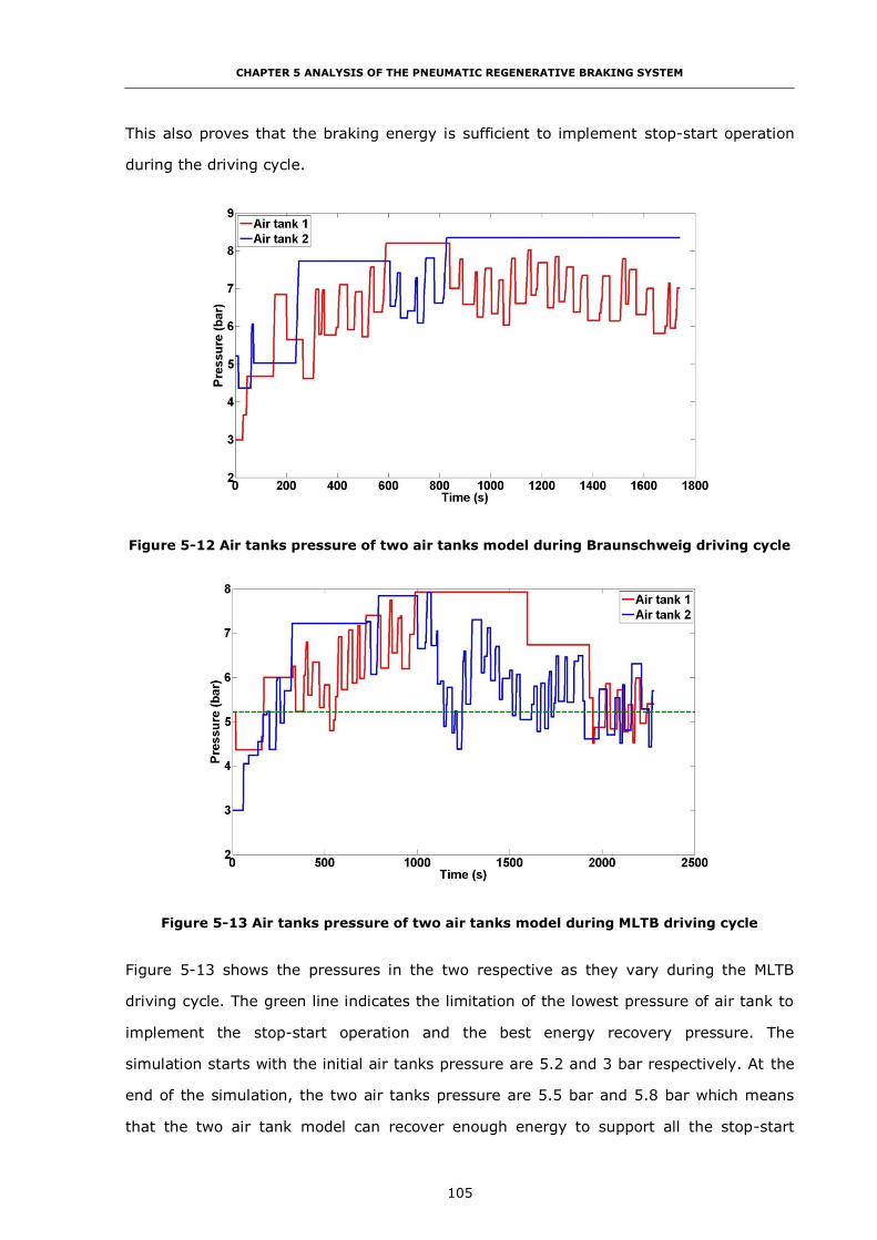
CHAPTER 5 ANALYSIS OF THE PNEUMATIC REGENERATIVE BRAKING SYSTEM
105
This also proves that the braking energy is sufficient to implement stop-start operation
during the driving cycle.
Figure 5-12 Air tanks pressure of two air tanks model during Braunschweig driving cycle
Figure 5-13 Air tanks pressure of two air tanks model during MLTB driving cycle
Figure 5-13 shows the pressures in the two respective as they vary during the MLTB
driving cycle. The green line indicates the limitation of the lowest pressure of air tank to
implement the stop-start operation and the best energy recovery pressure. The
simulation starts with the initial air tanks pressure are 5.2 and 3 bar respectively. At the
end of the simulation, the two air tanks pressure are 5.5 bar and 5.8 bar which means
that the two air tank model can recover enough energy to support all the stop-start

CHAPTER 5 ANALYSIS OF THE PNEUMATIC REGENERATIVE BRAKING SYSTEM
106
operations during the MLTB driving cycle. In addition, the lower air tank pressure results
in higher energy capture during the CM. As a result, the energy recovery potential of the
two air tanks system will be higher.
The simulation results with both the Braunschweig and MLTB driving cycles in Figure 5-12
and Figure 5-13 also demonstrates that the braking energy recovery rate relates to the
speed and number of stops of the vehicle. The Braunschweig driving cycle has less Stop–
Start operations which can produce a higher mass of recovered air per vehicle stop, so
can keep the pressure of air tank at a higher level compared with the MLTB driving cycle.
Figure 5-14 shows a comparison of air mass recovery of two air tanks over the
Braunschweig driving cycle. Tank 1 recover 2841.4 g and tank 2 recover 3536.1 g
respectively. Compared with the pressure at the start of the cycle, it can be found with a
lower initial pressure more air can be recovered in a single driving cycle because the
lower air tank pressure can enhance the net recovery of energy.
Figure 5-14 Air mass recovery during the Braunschweig driving cycle
Table 5-6 shows the comparison of air mass recovered during the Braunschweig driving
cycle between the new control strategy and the previous one in Chapter 4. The previous
initial air tanks pressure, 5.2 bar and 4.5 bar, is shown to recover 6377.5 g air, 171.4 g
less than the newly optimized initial air tanks pressure, 5.2 bar and 3 bar. This is
because the lower air tank pressure can recover more air mass during the braking which
is not only proved by the optimisation result, but also confirmed in Chapter 3. As a result,

CHAPTER 5 ANALYSIS OF THE PNEUMATIC REGENERATIVE BRAKING SYSTEM
107
the simulation starts with lower air tanks pressure can recover more air mass during the
braking. Although the increment is only 2.7%, it still proves that optimising the initial air
tanks pressure is worth doing for the research. This is because during the Braunschweig
driving cycle, the optimised control strategy still can support all the Stop-Start operations
which mean the air amount used to drive the air starter is not change. The 2.7%
increment all come from the energy recovery efficiency increased during the braking.
This means the optimisation of the initial air tanks pressure can increase the energy
recovery efficiency.
Table 5-6 Comparison of air mass recovered during Braunschweig driving cycle between
the new control strategy and the previous one
Air mass in the previous
control strategy (g)
Air mass in the new control Strategy
with optimisation result (g)
Start End Increment Start End Increment
Air mass in tank 1 (g)
840 3681.4 2841.4 840 2926.1 2086.1
Air mass in tank 2
(g) 500 4036.1 3536.1 500 4962.8 4462.8
Total air mass
recovered (g) - - 6377.5 - - 6548.9
Improvement (-) - - - - - 171.4
(2.7%)
5.7 Conclusion
This analysis of vehicle behaviour through different bus drive cycles and during braking
events, including a comparison of two configurations of the hybrid braking system points
to the fully controllable hybrid braking system is the focus of the investigation.
The funding includes
(i) It indicates that in the urban area the bus’s braking power can reach to 80% of
the total traction power, and the braking of the city bus is very gentle with most
of the deceleration rate below 0.2 g, compared with the passenger car.
(ii) The fully controllable hybrid braking system is fit for the requirement of the
pneumatic hybrid regenerative system which can either work at high efficiency

CHAPTER 5 ANALYSIS OF THE PNEUMATIC REGENERATIVE BRAKING SYSTEM
108
to recover as much braking energy as possible and supply the corresponding
braking force.
(iii) The optimisation result shows that the 5.2 bar air tank pressure is the best
pressure for braking energy recovery.
(iv) The model with the newly optimized initial air tanks pressure can enhance 2.7%
the total air mass recovered during the braking compared with the previous
control strategy which means the air tanks pressure is the function of the energy
recovery rate.
These findings give the fundamental fact for the future research to develop the
pneumatic hybrid city bus control strategy which not only can realize the Stop-Start
function, but also other functions such as Boost function which will be discussed in
Chapter 6.

CHAPTER 6 EVALUATING THE PERFORMANCE IMPROVEMENT OF PNEUMATIC REGENERATIVE SYSTEM
109
CHAPTER 6
EVALUATING THE PERFORMANCE IMPROVEMENT OF
PNEUMATIC REGENERATIVE SYSTEM
6.1 Introduction
Pneumatic hybrid technology refers to the use of storage of compressed air as a means
of energy recovery in a vehicle system. A pneumatic hybrid system stores compressed
air during the braking process. The compressed air can be re-used either to realize a
regenerative Stop-Start function or to improve the engine performance by injecting
compressed air into the inlet manifold to build-up engine torque more rapidly compared
with the unassisted engine [11].
This chapter theoretically analyses the reasons for engine turbo-lag and the methods
developed for reducing the turbo-lag and improving transient response first. Then, a
number of architectures for managing a rapid energy transfer into the powertrain to
assist acceleration of the turbocharger have been proposed and investigated from two
aspects, engine brake torque response and vehicle acceleration, by using the 1-D engine
simulation.
6.2 Theoretical Analysis of the Methods to Reduce Turbo-lag
As described in [11], the pneumatic hybrid technology has benefits that accrue from
using the stored compressed air to reduce turbo-lag. Turbo-lag is observed when the
engine load is increased. Increasing air flow to the cylinders is the result of a series of
energy transfers in the air system which requires time to stabilize. Consequently, the air-
fuel ratio falls since the air-supply cannot immediately match the increased fuelling that
corresponds to the load demand on the engine. To limit particulate emissions, the
quantity of fuel injected is controlled by a smoke limiting function implemented in the
engine management system and is adjusted to match the supply of fresh air [85]. As a
result, the engine spends longer at part load conditions so that both fuel consumption

CHAPTER 6 EVALUATING THE PERFORMANCE IMPROVEMENT OF PNEUMATIC REGENERATIVE SYSTEM
110
and exhaust emissions may be adversely affected. The response time of the air system
may be reduced either by directly increasing the air-supply to the cylinders or by directly
accelerating the turbocharger using an external torque source such as an electric motor
[86]. The direct supply of air, made possible in the pneumatic hybrid system, can rapidly
help develop the cylinder torque corresponding to a normal level of boost.
For the turbocharged diesel engine on the vehicular application, there are three
approaches to cope the turbo-lag problematic behaviour[86]:
(i) Controlling of the fuel flow.
(ii) Speeding up of the system (engine, manifolds and turbocharger) response.
(iii) Increasing of the number of transmission gears for vehicular applications.
The first method, controlling of the fuel flow, had been analysed in detail [86], as one
way to manage turbo-lag. It is recognized as a ‘passive’ method because the low air
supply and low injected fuel mass cause a slower engine response and poor vehicle
drivability. The third method, increasing of the number of transmission gears, has also
been considered as a ‘passive’ method for the reason that more gear ratios to make use
of the available torque worsen drivability owing to the much more frequent gear changes
required. Both first and third methods are intended to cure the symptom of black smoke
emission rather than the underlying cause of the turbocharger delay [86]. The second
method, speed-up of the system (engine, manifolds and turbochargers) response, is
considered an ‘active’ method in [86], because it improves the transient response of the
engine, manifolds and turbocharger. The focus of this chapter is on the realization of the
second method by use of stored compressed air during braking events.
An analysis of three system concepts is given. The systems are:
(i) Intake Boost System (System I),
(ii) Intake Port Boost System (System IP), and
(iii) Exhaust Boost System (System E).
Three proposed systems are considered first by integrating into a six cylinders 7.25 l
heavy-duty diesel engine (YUCHAI YC6A engine) respectively. The three concepts have
been respectively modelled in a 1-D engine code, and the performance changes,

CHAPTER 6 EVALUATING THE PERFORMANCE IMPROVEMENT OF PNEUMATIC REGENERATIVE SYSTEM
111
analysed in detail. First, when the engine accelerates from no load to full load at 1600
rpm, the development of brake torque has been compared and analysed. Then the
performances of respectively two different pneumatic hybrid city bus configurations
(Systems I and IP), have been considered. The acceleration capability of the two types of
vehicle has been simulated and the results compared.
6.3 Investigation of the Response Time Improvement
In general, when an additional load is applied to an engine, the current torque output of
the engine cannot instantly match the increased load requirement and as a result, the
engine speed drops. Note that a sophisticated feed-forward control could seek to match
fuelling and a predicted load, but there is always likely to be some mismatch. A speed
change is monitored by the engine controller which will increase the fuel injection mass
to increase engine speed. However, the turbocharger cannot instantly supply the
corresponding required air flow to the cylinders which tends to cause a reduction in the
air-fuel ratio. Therefore, the higher fuel mass and lower air supply tend to cause
inefficient combustion and insufficient exhaust gas energy to speed-up the turbocharger.
The two most prominent examples are respectively the vehicle climbing a hill or engaging
the clutch after a gear change.
The speed transient event normally happens when the driver requires a significant
acceleration. After the driver fully depresses the accelerator pedal, the engine controller
sends out the maximum fuel mass injection signal. Since the resistance torque remains
unchanged and the compressor air-supply cannot yet match the higher injected fuel
mass, the air-fuel ratio decreases as the air supply slowly increases. The low air-fuel ratio
in both load and speed increase transient events lead to poor combustion and
consequently increased particulate emissions and poor fuel economy.
6.3.1 Analysis of the Approaches to Improve Turbocharger Response
Time
In a turbocharged engine, there is no mechanical connection between the turbocharger
and the engine crankshaft. Therefore, turbocharger and engine speeds are coupled
through the gas dynamics of inlet and exhaust. The boost pressure and mass flow rate of
the compressor are related compressor map such as the one shown in Figure 6-1. The

CHAPTER 6 EVALUATING THE PERFORMANCE IMPROVEMENT OF PNEUMATIC REGENERATIVE SYSTEM
112
map is developed at steady state conditions and can be considered as a reasonable
approximation for transient conditions where changes propagate at the local speed of
sound. However, for significant transient changes, this information is supplemented by
both turbine maps and the dynamic behaviour of the turbocharger.
Figure 6-1 Typical map of aerodynamic type turbocharger compressor
From the compressor map, it can be seen that it is unrealistic for the turbocharger to
achieve both high boost pressure and air-mass flow rate at its low working speed. An
acceleration process is required to take the device from its low boost pressure and air-
mass flow rate operation point to its high load condition. To achieve the new operating
point, the turbine power must exceed the compressor power to speed-up the
turbocharger. The following differential equation describes the angular rotation of the
turbocharger shaft as a result of applied torques. All the mechanical losses are
encapsulated in the mechanical efficiency.
𝜂𝑚𝑇𝐶𝜏𝑇 − |𝜏𝐶| = 𝐺𝑇𝐶𝑑𝜔𝑇𝐶
𝑑𝑡 (6-1) [86]
where, tC – instantaneous value for the compressor indicated torque,
tT – instantaneous value for the turbine indicated torque,
ηmTC – turbocharger mechanical efficiency,

CHAPTER 6 EVALUATING THE PERFORMANCE IMPROVEMENT OF PNEUMATIC REGENERATIVE SYSTEM
113
GTC – turbocharger rotating inertia,
ωTC – turbocharger angular velocity.
From the Equation (6-1), it can be seen that to improve the transient response during a
demand for greater air flow, the approaches can be:
Approach 1: Increasing the turbine torque, means increasing or supplementing the tT,
Approach 2: Reducing the moment of inertia of turbocharger, means reducing the GTC,
Approach 3: Reducing the turbocharger shaft mechanical losses, means increasing the
ηmTC.
The overall target for these methods is to increase the turbocharger angular
acceleration, 𝑑𝜔𝑇𝐶
𝑑𝑡. Approach 2 and Approach 3 both relate to the turbocharger
configuration and have been analysed in detail in [86], and will not be covered in this
research. Furthermore, Approach 3 seems like an effective means to improve the
turbocharger transient response from theoretical analysis, but it can only offer small
scope for improvement. Some suggestions based on the Approach 2 and Approach 3 are
given in [86] and summarized as follows:
(i) Adopting lighter materials to reduce the turbocharger moment of inertia appears
straightforward since the machine aerodynamics is unchanged although
manufacturing costs may be increased.
(ii) Use of more than one small turbocharger instead of a single (larger) unit reduces
inertia, but represents a major increase in the system complexity.
(iii) Reduction of turbine (and compressor) rotor diameters respectively will strongly
influence turbocharger and, consequently, engine speed response.
Approach 1, increasing the turbine torque, is the key topic of this research and will be
discussed in detail. In order to increase the turbocharger transient response, two possible
solutions are:
Solution 1: Supplement the turbine torque using an additional torque input device on the
turbocharger shaft.
Solution 2: Increasing the amount of the available energy in the exhaust gas.

CHAPTER 6 EVALUATING THE PERFORMANCE IMPROVEMENT OF PNEUMATIC REGENERATIVE SYSTEM
114
Approach 1 will be analysed in detail in the following sections. Figure 6-2 shows a
classification of various methods of reducing turbo-lag. In this chapter, the methods in
the orange background are investigated, and the method in the blue background will be
briefly introduced as a reference here.
Figure 6-2 Classification of various method of reducing turbo-lag
Electric assistance for turbocharging is gaining in popularity, but is included here for
comparison purposes. This thesis would not present any further analysis, but recognise
that a detailed comparison on the basis of fuel economy and cost effectiveness is
warranted and may form an aspect of our continuing work.
6.3.2 Methods of Improving the Turbocharger Transient Response by
Increasing the Turbine Torque
The methods to improve the turbocharger transient response by increasing the turbine
torque can be implemented at the intake, exhaust or the turbocharger shaft itself.
The main mechanism of these methods to improve the turbocharger transient response is
shown in Figure 6-3.
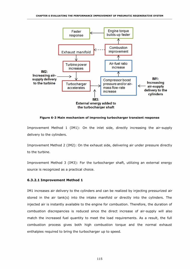
CHAPTER 6 EVALUATING THE PERFORMANCE IMPROVEMENT OF PNEUMATIC REGENERATIVE SYSTEM
115
Figure 6-3 Main mechanism of improving turbocharger transient response
Improvement Method 1 (IM1): On the inlet side, directly increasing the air-supply
delivery to the cylinders.
Improvement Method 2 (IM2): On the exhaust side, delivering air under pressure directly
to the turbine.
Improvement Method 3 (IM3): For the turbocharger shaft, utilizing an external energy
source is recognized as a practical choice.
6.3.2.1 Improvement Method 1
IM1 increases air delivery to the cylinders and can be realized by injecting pressurized air
stored in the air tank(s) into the intake manifold or directly into the cylinders. The
injected air is instantly available to the engine for combustion. Therefore, the duration of
combustion discrepancies is reduced since the direct increase of air-supply will also
match the increased fuel quantity to meet the load requirements. As a result, the full
combustion process gives both high combustion torque and the normal exhaust
enthalpies required to bring the turbocharger up to speed.

CHAPTER 6 EVALUATING THE PERFORMANCE IMPROVEMENT OF PNEUMATIC REGENERATIVE SYSTEM
116
Nowadays, increased engine ratings generally result in higher inlet manifold volumes,
hence slower response in the intake side [86]. Because the compressed air must both
increase the manifold pressure as well as increase air delivery to the cylinders, the
position at which air is injected into the intake manifold is an important factor in the
response improvement. The nature of the improvement brought about by IM1 is
apparent in Figure 6-3. IM 1 is closest of all the proposed changes to the combustion
process. As a result, IM1 should have the fastest air-supply increase and consequently
the greatest effect on response time.
One example of the implement of this method is the Pneumatic Boost System (PBS)
which is reported by Marx et al. in [85]. The PBS has been developed by the Knorr-
Bremse Company to realize a significant improvement in the response and acceleration
behaviour of the engine and the vehicle [85]. Figure 6-4 shows the system diagram for a
PBS equipped engine and the structure of the most important components of the system.
In normal operation where rates of change of engine condition are low, the engine’s air
demand is met by the turbocharger, during which time the PBS is in the rest position
with the flap fully opened and injection inactive (Figure 6-4, below left). In more dynamic
situations, when the turbocharger is not able to meet the engine’s air demand, the flap is
closed and air injection takes place (Figure 6-4, below right). The injection of air normally
ends when the pressure built up by the compressor in front of the closed flap has
reached the level of the pressure created by the PBS downstream of the flap. Both
pressures are measured continuously by the pressure sensors. From this point on, the
turbocharger is able to supply the engine with sufficient air.
Figure 6-5 shows a torque curve measured on an engine test bench with a spontaneous
torque request at idle speed. The engine, an 8 l diesel engine with EGR and two-stage
turbocharging, without PBS achieves 90% of its maximum torque in almost 5 s, whereas
the same engine with PBS achieves this value in 0.7 s [85].
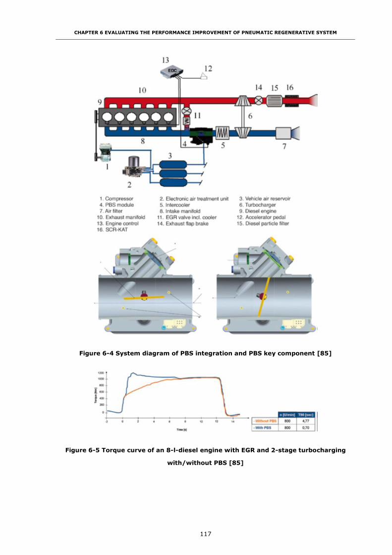
CHAPTER 6 EVALUATING THE PERFORMANCE IMPROVEMENT OF PNEUMATIC REGENERATIVE SYSTEM
117
Figure 6-4 System diagram of PBS integration and PBS key component [85]
Figure 6-5 Torque curve of an 8-l-diesel engine with EGR and 2-stage turbocharging
with/without PBS [85]

CHAPTER 6 EVALUATING THE PERFORMANCE IMPROVEMENT OF PNEUMATIC REGENERATIVE SYSTEM
118
6.3.2.2 Improvement Method 2
IM2 which increases the air-supply delivery to the turbine, can also be realized by
implementing the pneumatic hybrid technology to inject the compressed air into the
exhaust manifold as an additional flow of energy to the turbine. Air injection into the
exhaust manifold is less efficient than air injection into the intake manifold, since there is
still a lag between the intake and exhaust side. There is also the loss of availability
resulting from injection of relatively cool air into the exhaust manifold during the
acceleration process. Although the exhaust manifold pressure is increasing following the
boost in fuelling, the inertia of the turbocharger as well as the gas dynamics of filling the
intake manifold cause a further lag on the intake side. From Figure 6-3, it can be seen
that the IM2 is the most remote from combustion with changes having to propagate
through turbine, compressor and intake manifold.
An implementation of this method, the BRaking Exhaust Energy Storage (BREES) is
demonstrated in [87]. The experiments had been conducted by using a 2.0 l light-duty
diesel engine equipped with EGR and Variable Geometry Turbine (VGT) to evaluate the
engine transient response during in-gear braking and acceleration.
Figure 6-6 shows the system diagram for the BREES. It can be seen that to implement
the reported functions only a compressed gas tank, additional exhaust manifold
connection and a single control valve are necessary as shown in Figure 6-6.
Figure 6-6 System diagram of BREES [87]

CHAPTER 6 EVALUATING THE PERFORMANCE IMPROVEMENT OF PNEUMATIC REGENERATIVE SYSTEM
119
Figure 6-7 The effect of compressed air injection on brake torque and turbocharger
speed [87]
Figure 6-7 shows the effect of compressed air injection on brake torque and turbocharger
speed. It can be seen, the BREES system has a much sharper brake torque rise when the
conventional configuration clearly shows the turbo-lag between 24 to 28 second. Also,
the figure confirms the effectiveness of exhaust manifold injection to rapidly accelerate
the turbocharger, which was enabled between 24 and 26 second. Additional, the
experimental results confirm that the proposed system reduces the time to reach the
torque requirement during the 3rd gear tip-in by about 60% [87].
6.3.2.3 Improvement Method 3
With IM3, external energy added to the turbocharger shaft, can be realized by using
different kind of energy source such as electrical or hydraulic assistance.
One possible solution is Electric Assist Technology (EAT) using an electric motor mounted
on the turbocharger shaft. The motor offers additional torque to the turbocharger when a
load or speed increase is required. A schematic diagram of a diesel engine with
turbocharger EAT is shown in Figure 6-8.

CHAPTER 6 EVALUATING THE PERFORMANCE IMPROVEMENT OF PNEUMATIC REGENERATIVE SYSTEM
120
Figure 6-8 Schematic diagram of diesel engine with EAT
An alternative configuration makes use of an electric motor driving a separate
compressor which is installed upstream or downstream of its turbocharger counterpart in
an arrangement that resembles a combined supercharging scheme [86]. The schematic
diagram is shown in Figure 6-9.
Figure 6-9 Alternative combined supercharging configuration with electrically driven
compressor [86]
The Equation (6-1) described the relation between the normal, unassisted turbocharger
shaft torque and the turbocharger angular acceleration. For the turbocharger with the
electric motor assist, the respective balance is given by Equation (6-2).

CHAPTER 6 EVALUATING THE PERFORMANCE IMPROVEMENT OF PNEUMATIC REGENERATIVE SYSTEM
121
𝜂𝑚𝑇𝐶𝜏𝑇 + 𝜏𝐸𝑀 − |𝜏𝐶| = 𝐺𝑇𝐶+𝐸𝑀𝑑𝜔𝑇𝐶
𝑑𝑡 (6-2) [86]
where, tC – instantaneous value for the compressor indicated torque,
tT – instantaneous value for the turbine indicated torque,
tEM – electric motor torque,
ηmTC – turbocharger mechanical efficiency,
GTC+EM – combined turbocharger and EM mass moment inertia,
ωTC – turbocharger angular velocity.
For a successful integration of the electric motor, the established turbocharger shaft
acceleration must fulfil the following relation.
𝜂𝑚𝑇𝐶𝜏𝑇+𝜏𝐸𝑀−|𝜏𝐶|
𝐺𝑇𝐶+𝐸𝑀>
𝜂𝑚𝑇𝐶𝜏𝑇−|𝜏𝐶|
𝐺𝑇𝐶 (6-3) [86]
From Equation (6-3), the electric motor torque can be represented from Equation (6-4).
𝜏𝐸𝑀 >∆𝐺
𝐺𝑇𝐶(𝜂𝑚𝑇𝐶𝜏𝑇 − |𝜏𝐶|) (6-4)
where, tC – instantaneous value for the compressor torque,
tT – instantaneous value for the turbine torque,
tEM – electric motor torque,
ηmTC – turbocharger mechanical efficiency,
GTC – turbocharger rotating inertia,
∆𝐺 – increment of the rotating inertia.
Equation (6-4) indicated that when electric motor added to the turbocharger, the balance
of the motor torque and increment of shaft inertia, when the electric motor installed,
should be carefully considered.
There are two benefits to adopting the electric motor assist to the turbocharger.
Respectively, firstly the ability of the engine to operate at overall higher boost pressure
levels [86]. Secondly the electric motor not only can function also a turbocharger
accelerator, but also a generator. At low engine speed, when there is a load or speed
increase transient event, electric power is supplied to the turbocharger shaft aiding its
fast acceleration. At high engine speed, instead of wasting the energy that exceeds the
compressor requirement, the electric motor can convert to the electricity generator to

CHAPTER 6 EVALUATING THE PERFORMANCE IMPROVEMENT OF PNEUMATIC REGENERATIVE SYSTEM
122
recover the energy and store in energy storage such as a battery or a supercapacitor.
But the EAT has same disadvantages that prevent widespread application at low cost.
First is a more complex control system which includes the control strategy of the electric
motor. Second is the durability and reliability of the turbocharger remain to be proven.
6.4 Using Pneumatic Hybrid Technology to Improve the
Turbocharger Transient Response
6.4.1 Introduction of Reducing Turbo-lag by Using Pneumatic Hybrid
Technology
As mentioned before, increasing the air supply to the cylinders or to the turbine both can
be considered as effective methods to improve the engine transient response. The
pneumatic hybrid boost systems have inherent advantages to implement these methods
above to improve the transient response because of the ready availability of an air supply.
The air stored in the air tank(s) can be reused to improve turbocharger response time by
injecting air into the intake or exhaust manifold. To realize the Boost Function, there are
two different engine structures can be considered as candidates.
The first proposed structure, Intake Side Boost (ISB), is a realisation of IM1. In order to
increase the air-supply to the cylinders for combustion, the air can be injected into the
intake at different points such as the intake manifold or the intake ports. An example of
ISB is shown in Figure 6-10, in which the compressed air stored in the air tank is
supplied to the cylinders through the intake manifold at the time when acceleration of the
turbocharger is required. When the load or speed demand is made, the compressed air is
injected into the intake manifold in order to match the increased fuel injection mass. The
precise air flow is controlled by the Air Tank Valve (ATV). The Intake Manifold Valve (IMV)
will fully close during the injection period to prevent the compressed air being injected
back to the compressor. Because the air can be immediately used to support combustion
in the cylinders, the resulting high exhaust gas energy causes a faster turbocharger and
engine response to reduce turbo-lag. In order to avoid the compressor enter an unstable
operation condition, two methods can be implemented. The first is when the pressure of
the volume between the IMV and compressor reaches a threshold value, the IMV will
open to avoid the stall condition of the compressor. The second method is to set a
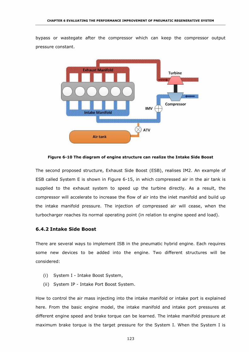
CHAPTER 6 EVALUATING THE PERFORMANCE IMPROVEMENT OF PNEUMATIC REGENERATIVE SYSTEM
123
bypass or wastegate after the compressor which can keep the compressor output
pressure constant.
Figure 6-10 The diagram of engine structure can realize the Intake Side Boost
The second proposed structure, Exhaust Side Boost (ESB), realises IM2. An example of
ESB called System E is shown in Figure 6-15, in which compressed air in the air tank is
supplied to the exhaust system to speed up the turbine directly. As a result, the
compressor will accelerate to increase the flow of air into the inlet manifold and build up
the intake manifold pressure. The injection of compressed air will cease, when the
turbocharger reaches its normal operating point (in relation to engine speed and load).
6.4.2 Intake Side Boost
There are several ways to implement ISB in the pneumatic hybrid engine. Each requires
some new devices to be added into the engine. Two different structures will be
considered:
(i) System I - Intake Boost System,
(ii) System IP - Intake Port Boost System.
How to control the air mass injecting into the intake manifold or intake port is explained
here. From the basic engine model, the intake manifold and intake port pressures at
different engine speed and brake torque can be learned. The intake manifold pressure at
maximum brake torque is the target pressure for the System I. When the System I is

CHAPTER 6 EVALUATING THE PERFORMANCE IMPROVEMENT OF PNEUMATIC REGENERATIVE SYSTEM
124
working, the sensor will detect the intake manifold pressure. Once the pressure reaches
the target pressure, the System I will stop injecting the air from air tank. The System IP
uses the intake port pressure as the target pressure. The reason for choosing this control
algorithm is to keep the control system simple. And it will not change the air mass
injected to the engine and the air inlet behaviours of the engine.
6.4.2.1 System I
Figure 6-11 shows the arrangement of equipment with some new devices added to the
original pneumatic hybrid engine structure that was first shown in [11]. The original
pneumatic hybrid engine devices like the air tank, compression release engine braking
device, air tank, air motor, check valve and throttle valve are retained. The new devices
are respectively the connection pipes between the air tank and the intake manifold with
the ATV1, and the IMV in the intake manifold downstream of the intercooler. The IMV is
to prevent the compressed air being injected back to the compressor. Such an increasing
pressure has the tendency to move the compressor operating point towards surge.
Figure 6-11 System diagram of System I
In normal operation, when the engine does not require high air demand and the
compressor can supply enough pressure, both IMV and TVs, fully open to let the engine
operate in the normal turbocharged mode.
When the compressor cannot supply enough air to the engine in a highly dynamic
situation like acceleration or on steep gradients, System I is activated. The high pressure

CHAPTER 6 EVALUATING THE PERFORMANCE IMPROVEMENT OF PNEUMATIC REGENERATIVE SYSTEM
125
air from the air tank injects into the manifold through the ATV1. The IMV closes and TVs
fully open. The injection of air ends when the compressor delivery pressure is higher than
the pressure of the injected air. At this point, IMV opens and ATV1 closes.
The injection of the air from the air tank only requires a short period of operation,
because after few engine cycles, the turbocharger will accelerate to a normal operating
speed. As a result, the compressor can supply sufficient air to the engine to realise a
satisfactory acceleration. The time to reach maximum torque is significantly reduced.
Rakopoulos et al. [86] reported that, for a 0 to 60% load acceptance aided by a 2 s air-
injection duration right after the onset of the transient event, the engine response time
was approximately halved in a medium-speed, turbocharged diesel engine rated at 1410
bhp at 750 rpm in Figure 6-12. Furthermore, for an air-injection assist on a six-cylinder,
turbocharged diesel of 11.32 l displacement volume revealed a reduction in the time
period with peak smoke from 3 to 0.5 s as well as improvement in the speed response
from 4 to 1.5 s for severe load acceptance transient at 1000 rpm [86].
Figure 6-12 Effect of air-injection on transient response after a load step of 60% full-
load [86]
An alternative way of presenting the transient response improvement made by the
different pneumatic hybrid technologies are depicting in on the turbocharger compressor
map compared with the normal engine without any response improvement methods
which are illustrated in Figure 6-13. Normally, turbo-lag happens at the early stage of the
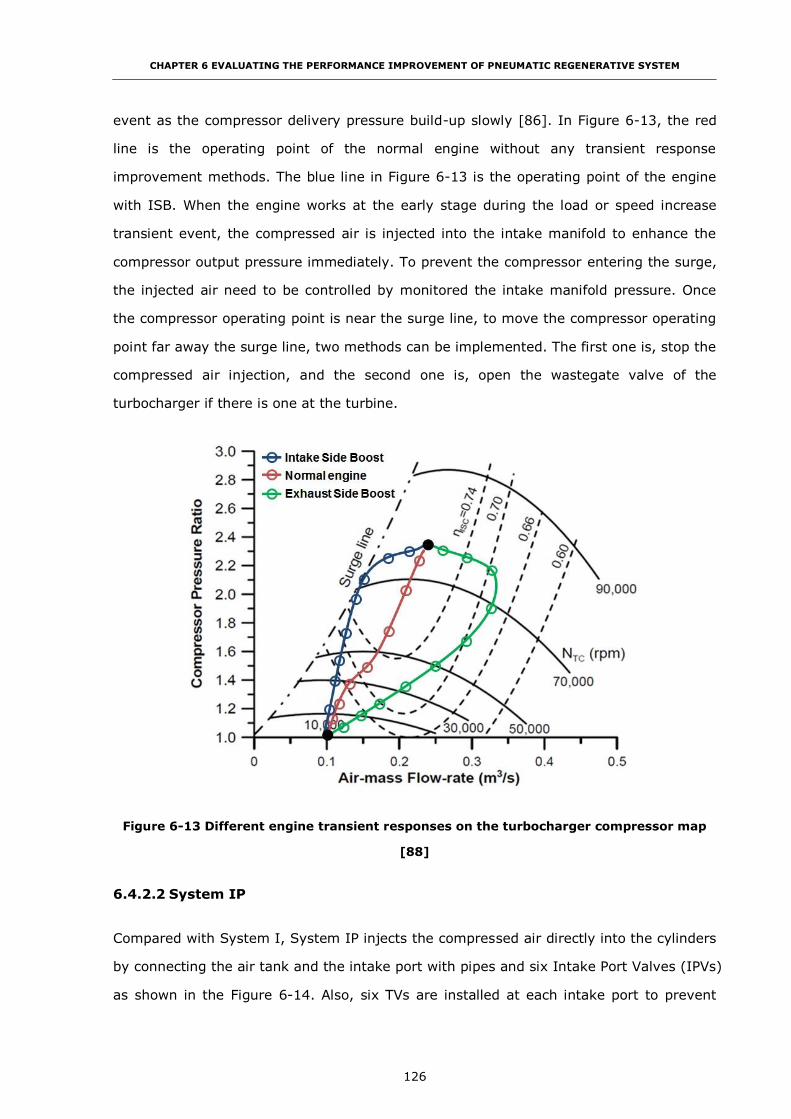
CHAPTER 6 EVALUATING THE PERFORMANCE IMPROVEMENT OF PNEUMATIC REGENERATIVE SYSTEM
126
event as the compressor delivery pressure build-up slowly [86]. In Figure 6-13, the red
line is the operating point of the normal engine without any transient response
improvement methods. The blue line in Figure 6-13 is the operating point of the engine
with ISB. When the engine works at the early stage during the load or speed increase
transient event, the compressed air is injected into the intake manifold to enhance the
compressor output pressure immediately. To prevent the compressor entering the surge,
the injected air need to be controlled by monitored the intake manifold pressure. Once
the compressor operating point is near the surge line, to move the compressor operating
point far away the surge line, two methods can be implemented. The first one is, stop the
compressed air injection, and the second one is, open the wastegate valve of the
turbocharger if there is one at the turbine.
Figure 6-13 Different engine transient responses on the turbocharger compressor map
[88]
6.4.2.2 System IP
Compared with System I, System IP injects the compressed air directly into the cylinders
by connecting the air tank and the intake port with pipes and six Intake Port Valves (IPVs)
as shown in the Figure 6-14. Also, six TVs are installed at each intake port to prevent

CHAPTER 6 EVALUATING THE PERFORMANCE IMPROVEMENT OF PNEUMATIC REGENERATIVE SYSTEM
127
compressed air being injected back into the compressor. A high pressure common air rail
connects ATV1 and IPVs on each intake port.
Figure 6-14 System diagram of System IP
In the normal operation, when the engine does not require high air demand and the
compressor can supply enough pressure, the TVs fully open while the IPVs and ATV1 fully
close.
During an engine transient when the compressor is unable to supply enough air to the
engine, System IP is activated. The high pressure air from the air tank is injected into the
high pressure air rail through ATV1, and in turn the air is injected into the cylinder by
means of the IPVs. The TVs on each intake port fully close during the injection. The
injection will end when the pressure that the compressor builds is higher than the
pressure of the injected air. The TVs fully open again and the IPVs close.
According to where the compressed air is injected into the intake manifold the dynamics
of the air supply change. Pressurising the whole manifold compared with supplying air to
the inlet ports will be a slower, but more complex in the mechanical design. Compared
with System I, System IP can deliver the compressed air more quickly since it only needs
fill a small volume auxiliary chamber between the TV, IPV and intake valve in each intake
port. Moreover, System IP allows the compressor to accelerate to its normal operating
condition without risking surge or stall. Only one intake port is blocked by the TV during
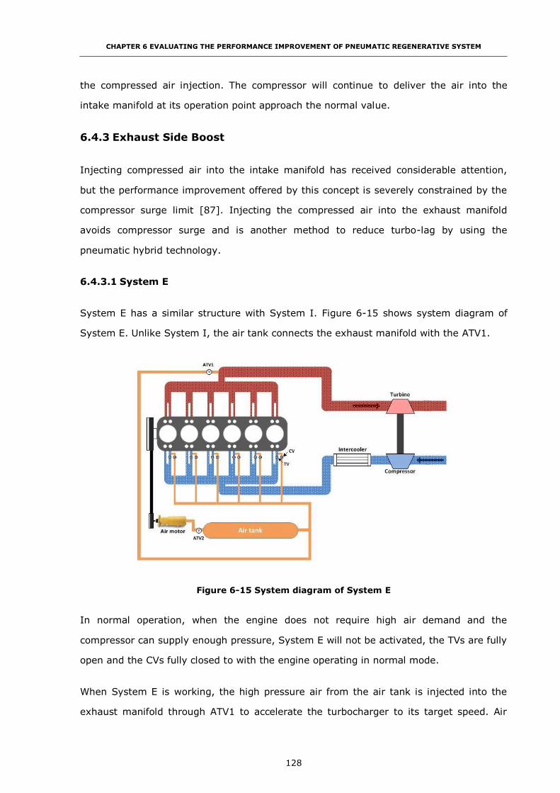
CHAPTER 6 EVALUATING THE PERFORMANCE IMPROVEMENT OF PNEUMATIC REGENERATIVE SYSTEM
128
the compressed air injection. The compressor will continue to deliver the air into the
intake manifold at its operation point approach the normal value.
6.4.3 Exhaust Side Boost
Injecting compressed air into the intake manifold has received considerable attention,
but the performance improvement offered by this concept is severely constrained by the
compressor surge limit [87]. Injecting the compressed air into the exhaust manifold
avoids compressor surge and is another method to reduce turbo-lag by using the
pneumatic hybrid technology.
6.4.3.1 System E
System E has a similar structure with System I. Figure 6-15 shows system diagram of
System E. Unlike System I, the air tank connects the exhaust manifold with the ATV1.
Figure 6-15 System diagram of System E
In normal operation, when the engine does not require high air demand and the
compressor can supply enough pressure, System E will not be activated, the TVs are fully
open and the CVs fully closed to with the engine operating in normal mode.
When System E is working, the high pressure air from the air tank is injected into the
exhaust manifold through ATV1 to accelerate the turbocharger to its target speed. Air

CHAPTER 6 EVALUATING THE PERFORMANCE IMPROVEMENT OF PNEUMATIC REGENERATIVE SYSTEM
129
injection ends when the intake manifold pressure reaches its normal working pressure
according to engine speed and load.
From this analysis, it can be observed that System E is least effective of the methods
under review because of the long process path apparent from the process diagram for
boost, Figure 6-3. But it has a substantial advantage that the compressor operating point
is reached without risk of surge or stall.
6.5 Engine with Pneumatic Hybrid Boost System Simulation Models
and Result
6.5.1 Basic Engine Simulation Model
To simulate the transient response improvement made by three different pneumatic
hybrid boost systems, respectively Systems I, IP and E, a 1-D engine simulation code,
GT-POWER, is used to simulate the engine performance when a load transient is applied
to the engine.
A heavy-duty, six cylinders, turbocharged & intercooler diesel engine based on the
YUCHAI YC6A Series engine is modelled in GT-POWER as shown below in Figure 6-16.
The Information of the GT-POWER models in this research is introduced in detail in
Appendix-II. The YC6A series diesel engine is a new type turbocharged & intercooler
diesel engine co-developed by YUCHAI in China, and FEV Company in Germany [89]. The
main technical parameters of YC6A series engines are shown in Table 6-1.
Here, the YC6A240-30 is chosen as the base engine for the study. Its GT-POWER engine
model which includes a ‘DIWiebe’ combustion sub model and a ‘WoschniGT’ heat transfer
sub model is shown in Figure 6-16. The ‘DIWiebe’ model imposes the combustion burn
rate for direct-injection, compression-ignition engines using a three-term Wiebe function,
and is used to define the injection system, cylinder geometry, valve lift and valve timing
[90]. ‘WoschniGT’ indicates that the in-cylinder heat transfer will be calculated by a
formula which closely emulates the classical Woschni correlation without swirl [91]. Both
‘DIWiebe’ and ‘WoschniGT’ models are introduced in detail in Appendix-III.
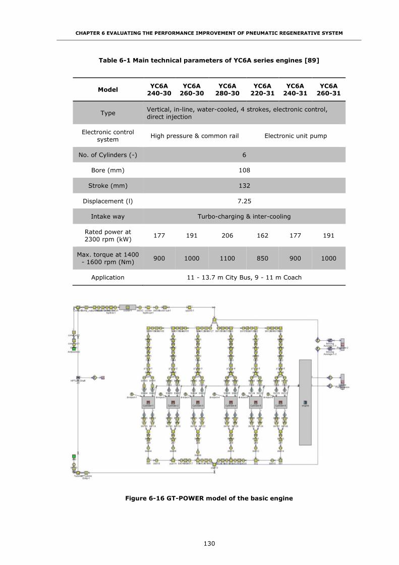
CHAPTER 6 EVALUATING THE PERFORMANCE IMPROVEMENT OF PNEUMATIC REGENERATIVE SYSTEM
130
Table 6-1 Main technical parameters of YC6A series engines [89]
Model YC6A
240-30 YC6A
260-30 YC6A
280-30 YC6A
220-31 YC6A
240-31 YC6A
260-31
Type Vertical, in-line, water-cooled, 4 strokes, electronic control,
direct injection
Electronic control
system High pressure & common rail Electronic unit pump
No. of Cylinders (-) 6
Bore (mm) 108
Stroke (mm) 132
Displacement (l) 7.25
Intake way Turbo-charging & inter-cooling
Rated power at
2300 rpm (kW) 177 191 206 162 177 191
Max. torque at 1400
- 1600 rpm (Nm) 900 1000 1100 850 900 1000
Application 11 - 13.7 m City Bus, 9 - 11 m Coach
Figure 6-16 GT-POWER model of the basic engine

CHAPTER 6 EVALUATING THE PERFORMANCE IMPROVEMENT OF PNEUMATIC REGENERATIVE SYSTEM
131
6.5.2 Simulation of the Engine with System I
Figure 6-17 shows the GT-POWER model of the engine with System I. Compared with the
basic engine model, some new modules, ISystem-Control-Unit (highlighted in green),
and pneumatic hybrid system (highlighted in red) are added into the model. The
pneumatic hybrid system includes one air tank, pipes, one air tank valve and an intake
manifold valve. The check valves and throttle valves at each intake port, as shown in the
Figure 6-11 are removed here because, the function of these valves is to recover the air
when the engine is working in compressor mode during braking (see [11]). In this
simulation model, only the ability of System I to improve engine performance aspect is
investigated. Other components, not included in the simulation of this function are
excluded from the model.
Figure 6-17 GT-POWER model of the engine with System I
The purpose of this simulation model is to investigate first the feasibility and then the
performance capability of System I. Also the simulation result will be compared with
other kinds of pneumatic hybrid boost system. The dimensions and characteristics of
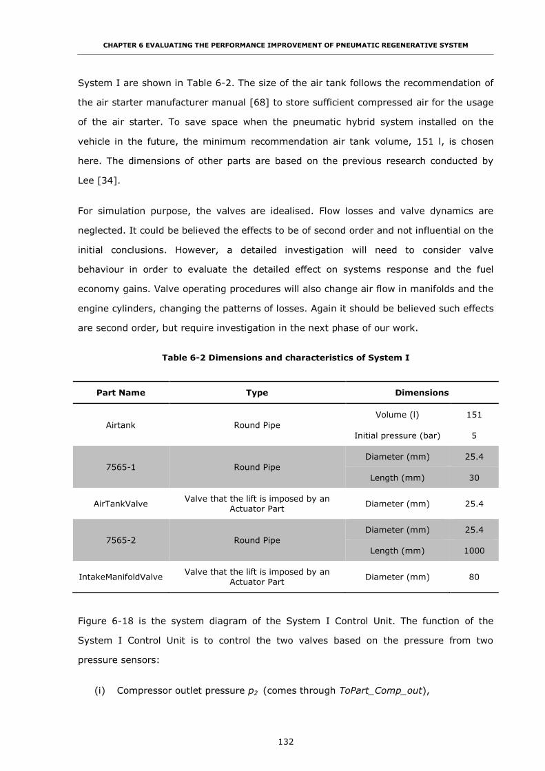
CHAPTER 6 EVALUATING THE PERFORMANCE IMPROVEMENT OF PNEUMATIC REGENERATIVE SYSTEM
132
System I are shown in Table 6-2. The size of the air tank follows the recommendation of
the air starter manufacturer manual [68] to store sufficient compressed air for the usage
of the air starter. To save space when the pneumatic hybrid system installed on the
vehicle in the future, the minimum recommendation air tank volume, 151 l, is chosen
here. The dimensions of other parts are based on the previous research conducted by
Lee [34].
For simulation purpose, the valves are idealised. Flow losses and valve dynamics are
neglected. It could be believed the effects to be of second order and not influential on the
initial conclusions. However, a detailed investigation will need to consider valve
behaviour in order to evaluate the detailed effect on systems response and the fuel
economy gains. Valve operating procedures will also change air flow in manifolds and the
engine cylinders, changing the patterns of losses. Again it should be believed such effects
are second order, but require investigation in the next phase of our work.
Table 6-2 Dimensions and characteristics of System I
Part Name Type Dimensions
Airtank Round Pipe
Volume (l) 151
Initial pressure (bar) 5
7565-1 Round Pipe
Diameter (mm) 25.4
Length (mm) 30
AirTankValve Valve that the lift is imposed by an
Actuator Part Diameter (mm) 25.4
7565-2 Round Pipe
Diameter (mm) 25.4
Length (mm) 1000
IntakeManifoldValve Valve that the lift is imposed by an
Actuator Part Diameter (mm) 80
Figure 6-18 is the system diagram of the System I Control Unit. The function of the
System I Control Unit is to control the two valves based on the pressure from two
pressure sensors:
(i) Compressor outlet pressure p2 (comes through ToPart_Comp_out),

CHAPTER 6 EVALUATING THE PERFORMANCE IMPROVEMENT OF PNEUMATIC REGENERATIVE SYSTEM
133
(ii) Pressure downstream of the IMV (comes through ToPart_506) – which in turn
becomes the target pressure for a control loop controlling ATV lift.
Figure 6-18 System diagram of System I control-unit
Based on the results of comparing the pressures of two positions mentioned before, the
ISystem-Control-Unit will control the two valves. The flow chart of System I control
strategy is also shown in Figure 6-19.
Figure 6-19 Flow chart of the System I control strategy

CHAPTER 6 EVALUATING THE PERFORMANCE IMPROVEMENT OF PNEUMATIC REGENERATIVE SYSTEM
134
(i) If the air tank pressure is sufficient to boost the engine, which means the air
tank pressure pAT is greater than the limit pressure pL, and the compressor is
unable to supply the target boost pressure pT (p2 < pT), System I will be
activated. The control unit will open the Air Tank Valve to inject compressed air
into the manifold, while the Intake Manifold Valve will be closed. When p2 is
greater than the IMV opening threshold pressure pt, the IMV will open to prevent
the compressed air causing compressor a surge. The system will be turned off
and the ATV will be closed until the intake manifold pressure reaches the target
boost pressure.
(ii) If the air tank pressure is not sufficient, which means the air tank pressure pAT is
less than the limit pressure pL, to boost the engine the control unit will not
activate System I. As a result, the ATV will be closed and the IMV will be opened
to supply air to the cylinders.
6.5.3 Simulation of the Engine with System IP
Figure 6-20 GT-POWER model of the engine with System IP
As shown in the Figure 6-20, some new modules, IPSystem-Control-Unit (highlighted in
green), and pneumatic hybrid system (highlighted in red) are added to the basic engine

CHAPTER 6 EVALUATING THE PERFORMANCE IMPROVEMENT OF PNEUMATIC REGENERATIVE SYSTEM
135
model. The system includes one air tank, pipework, a single ATV, six IPVs and six TVs.
The ATV and six IPVs are connected to using a high pressure air rail.
When System IP is activated, the high pressure air from the air tank is injected into the
high pressure air rail through the ATV. In turn, the air will be injected into the cylinder by
means of the IPVs. The function of the TVs on each intake port is to prevent the
compressed air leaking back into the inlet manifold. The injection will end when the
pressure that the compressor builds is higher than the pressure of the injected air. The
TVs will fully open again and the IPVs will close.
The dimensions and characteristics of System IP are shown in Table 6-3. The air tank is
kept at the same volume for consistency. Other design parameters are same as the
System I.
Table 6-3 Dimensions and characteristics of System IP
Name Type Dimensions
Air Tank Round Pipe
Volume (l) 151
Initial pressure (bar) 5
7565-2 Round Pipe
Diameter (mm) 25.4
Length (mm) 1000
Air Tank Valve Valve that the lift is imposed by an
Actuator Part Diameter (mm) 25.4
7565-1 Round Pipe
Diameter (mm) 25.4
Length (mm) 30
Intake Port Valve 1-6 Valve that the lift is imposed by an
Actuator Part Diameter (mm) 12.7
Yjun2
A spherical-shaped flow split volume
connected to one or more flow components
Diameter (mm) 45.7
7016,7020,7021,7031
,7037,7043 Round Pipe
Diameter (mm) 32.4
Length (mm) 60
Throttle Valve 1-6 Throttle that the throttle angle is imposed
by an Actuator Part Diameter (mm) 32.4

CHAPTER 6 EVALUATING THE PERFORMANCE IMPROVEMENT OF PNEUMATIC REGENERATIVE SYSTEM
136
Figure 6-21 System diagram of System IP control-unit
Figure 6-21 is the system diagram of the System IP Control Unit. Compared with System
I, the deployment of the pressure sensors is changed:
(i) Compressor outlet pressure p2 (comes through ToPart_Comp_out),
(ii) Exhaust manifold pressure p3 (comes through ToPart_HPTurbineEntry-1).
Measurement of p3 is required because when System IP is working, the compressed air is
injected into the small chamber composed by the IV, TV and intake valve in each intake
port, the intake manifold pressure does not behave as in Systems I. Based on the
pressure measurements, the valves are controlled to facilitate two operating modes. The
flow chart of System IP control strategy is shown in Figure 6-22.
(i) If the air tank pressure pAT is greater than the limit pressure pL, which means the
air tank pressure is sufficient to boost the engine, and at the same time, the
compressor is unable to supply the target boost pressure, which means the
turbine input pressure p3 is less than the target exhaust manifold pressure pE,
System IP will be activated. The control unit will open the ATV and the IPVs to
inject compressed air into the cylinders, while the TVs in the intake ports will be
closed to prevent the compressed air leaking back into the inlet manifold. When
the compressor outlet pressure p2 is greater than the TVs opening threshold
pressure pt, the TVs will fully open. System IP will be turned off when p3 is
greater than pE, and the ATV and IPVs will be closed.
(ii) If the air tank pressure is not sufficient to boost the engine, which means the air
tank pressure pAT is less than the limit pressure pL, whether the compressor can
supply the target boost pressure or not, the control unit will not activate System

CHAPTER 6 EVALUATING THE PERFORMANCE IMPROVEMENT OF PNEUMATIC REGENERATIVE SYSTEM
137
IP. As a result, the ATV and IPVs will be closed and all six TVs will be opened to
supply the air flow to the cylinders.
Figure 6-22 Flow chart of the System IP control strategy
6.5.4 Simulation of the Engine with System E
New modules, ESystem-Control-Unit (highlighted in green), and pneumatic hybrid
system (highlighted in red) are added into the basic engine model to realise System E as
shown in the Figure 6-23. The pneumatic hybrid system includes one air tank, one ATV
and pipework connected the air tank with the exhaust manifold.
The dimensions and characteristics of System E are shown in the Table 6-4. The size of
the air tank, pipes and ATV are the same as used for the Systems I and IP to maintain
consistency.

CHAPTER 6 EVALUATING THE PERFORMANCE IMPROVEMENT OF PNEUMATIC REGENERATIVE SYSTEM
138
Figure 6-23 GT-POWER model of the engine with System E
Table 6-4 Dimensions and characteristics of System E
Name Type Dimensions
Air Tank Round Pipe
Volume (l) 151
Initial pressure (bar) 5
7565-2 Round Pipe
Diameter (mm) 25.4
Length (mm) 1000
Air Tank Valve Valve that the lift is imposed by an
Actuator Part Diameter (mm) 25.4
PipeRound-1 Round Pipe
Diameter (mm) 25.4
Length (mm) 30
FlowSplitSpher-1
A spherical-shaped flow split volume
connected to one or more flow components
Diameter (mm) 54

CHAPTER 6 EVALUATING THE PERFORMANCE IMPROVEMENT OF PNEUMATIC REGENERATIVE SYSTEM
139
Figure 6-24 is the system diagram of the System E Control Unit. The function of the
System E Control Unit is to control the ATV in System E. During a transient System E is
activated. The System E Control Unit uses two sensors to detect the pressures in the
system:
(i) Compressor outlet pressure p2 (comes through ToPart_Comp_out),
(ii) Exhaust manifold pressure p3 (comes through ToPart_yjun13).
Figure 6-24 System diagram of System E control-unit
Similar to System IP, the exhaust manifold pressure had been chosen as the set point for
control of the ATV opening. The ATV opening is controlled to facilitate two operating
modes. The flow chart of System E control strategy is also shown in Figure 6-25.
(i) If the air tank pressure pAT is greater than the limit pressure pL, the air tank
pressure is sufficient to boost the engine. If at the same time, the compressor is
unable to supply the target boost pressure (turbine input pressure p3 less than
the target exhaust manifold pressure PE), System E will be activated and the
control unit will open the ATV to inject compressed air into the exhaust manifold
to speed-up the turbocharger. When the exhaust manifold pressure p3 is equal or
greater than the target exhaust manifold pressure pE, the ATV will fully close.
(ii) If the air tank pressure is not sufficient to boost the engine, which means the air
tank pressure pAT is less than the limit pressure pL, the control unit will not
activate the controller. As a result, the ATV will remain fully closed.

CHAPTER 6 EVALUATING THE PERFORMANCE IMPROVEMENT OF PNEUMATIC REGENERATIVE SYSTEM
140
Figure 6-25 Flow chart of the System E control strategy
6.5.5 Engine with Pneumatic Hybrid Boost System Simulation Result
In this section, the maximum achievable performance from the three candidate
pneumatic hybrid boost systems are compared for the situation when the engine
accelerates from no load to full load at 1600 rpm. The obvious baseline for the result is
the performance of the basic engine without any pneumatic hybrid boost system. The
evaluation is done from each of three aspects.
(i) Engine performance improvement,
(ii) Air usage during the boost period,
(iii) Turbocharger operation condition.
6.5.5.1 Engine Performance Improvement
Figure 6-26 shows the simulated full load acceleration response of the engine in the
terms of engine brake torque. In the basic engine without any pneumatic hybrid boost

CHAPTER 6 EVALUATING THE PERFORMANCE IMPROVEMENT OF PNEUMATIC REGENERATIVE SYSTEM
141
system, torque can be seen to rise very slowly to reach the peak torque. The three
pneumatic hybrid boost system all have a much sharper brake torque rise. Table 6-5
gives the time taken in each case to reach its peak torque output and their improvement
to the basic engine performance expressed as the % reduction in response time.
Figure 6-26 Brake torque response for each pneumatic hybrid boost system
Table 6-5 Time to reach peak torque output of the four engine configurations
Time to 90% peak torque output
(s)
Improvement
(-)
Basic engine 1.15 -
Engine with System I 0.25 78.3%
Engine with System IP 0.42 63.5%
Engine with System E 0.45 60.9%
From Figure 6-26, it can be seen that Systems I and IP both have the fastest response in
the very earliest stages of the acceleration while the engine with System E shows a
decrease in brake torque output in this period. Such a decrease is likely to have an effect
on drivability and represents a serious shortcoming. The reason is because in the engine
with System E the whole manifold requires to be brought to its normal working pressure,
slowing the response. Also the cold air in the air tank injected to the exhaust manifold

CHAPTER 6 EVALUATING THE PERFORMANCE IMPROVEMENT OF PNEUMATIC REGENERATIVE SYSTEM
142
reduces the available energy in the exhaust gas which decreases the energy to the
turbine. As a result, it will decrease the air delivery to the cylinder which causes a drop in
the brake torque output. These results also support the hypothesis that the location of air
injection is fundamental to the result. It also can be seen in Figure 6-26 (inset) that
compared with System I, the engine with System IP has the faster initial brake torque
response because the compressed air is more quickly delivered to the cylinders in the
first few cycles. Finally System I gives the shortest time to reach maximum brake torque.
Figure 6-27 Intake manifold pressure for each pneumatic hybrid boost system
Figure 6-27 shows the intake manifold pressure change during the full-load acceleration
at an engine speed 1600rpm for each of the four engine configurations. The engine with
System I sees a rapid increase in intake manifold pressure. Once the engine with System
E has reached normal turbocharger operating conditions, it has the same ability to
increase the intake manifold pressure. The reason that System IP is slower to build inlet
manifold pressure is because as System IP simply needs less air from storage to achieve
the changed state of the turbocharger. It remains that System IP still demonstrates a
much faster intake manifold pressure build-up compared with the basic engine.
6.5.5.2 Air Usage during the Boost Period
Figure 6-28 shows the air tank pressure drop for one full-load acceleration. The reason
for the engine with System E using the least air is because the System E needs minimum
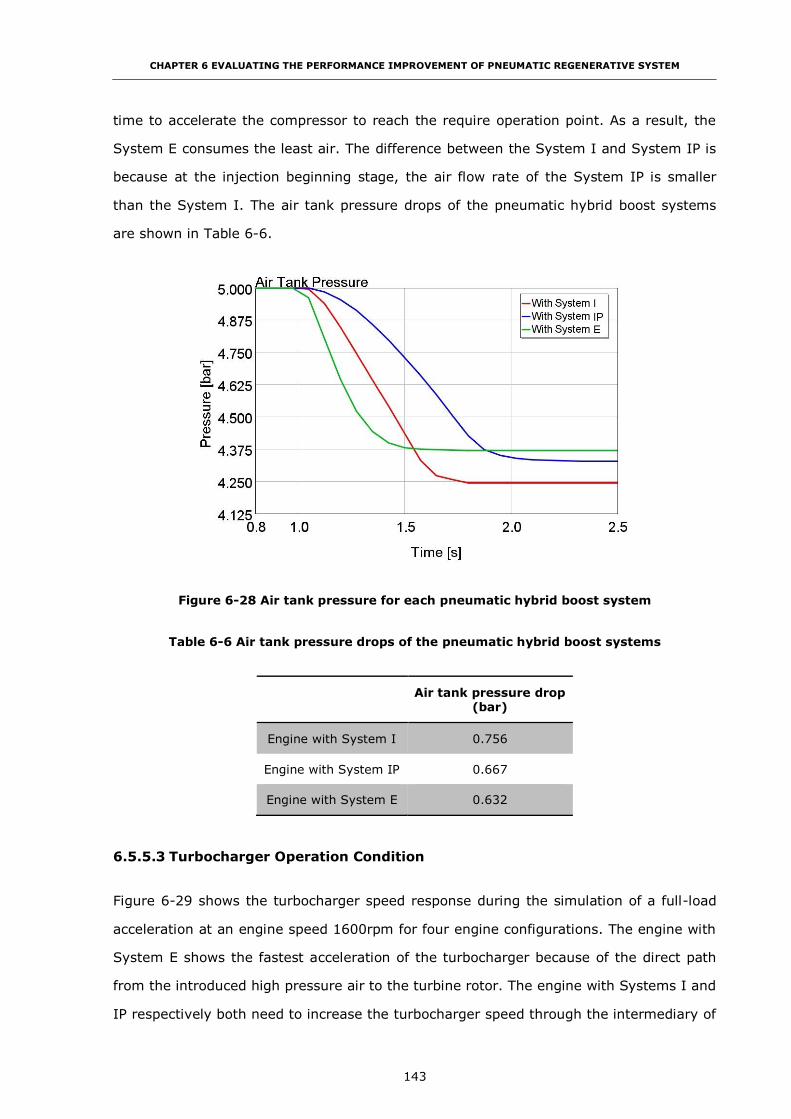
CHAPTER 6 EVALUATING THE PERFORMANCE IMPROVEMENT OF PNEUMATIC REGENERATIVE SYSTEM
143
time to accelerate the compressor to reach the require operation point. As a result, the
System E consumes the least air. The difference between the System I and System IP is
because at the injection beginning stage, the air flow rate of the System IP is smaller
than the System I. The air tank pressure drops of the pneumatic hybrid boost systems
are shown in Table 6-6.
Figure 6-28 Air tank pressure for each pneumatic hybrid boost system
Table 6-6 Air tank pressure drops of the pneumatic hybrid boost systems
Air tank pressure drop
(bar)
Engine with System I 0.756
Engine with System IP 0.667
Engine with System E 0.632
6.5.5.3 Turbocharger Operation Condition
Figure 6-29 shows the turbocharger speed response during the simulation of a full-load
acceleration at an engine speed 1600rpm for four engine configurations. The engine with
System E shows the fastest acceleration of the turbocharger because of the direct path
from the introduced high pressure air to the turbine rotor. The engine with Systems I and
IP respectively both need to increase the turbocharger speed through the intermediary of
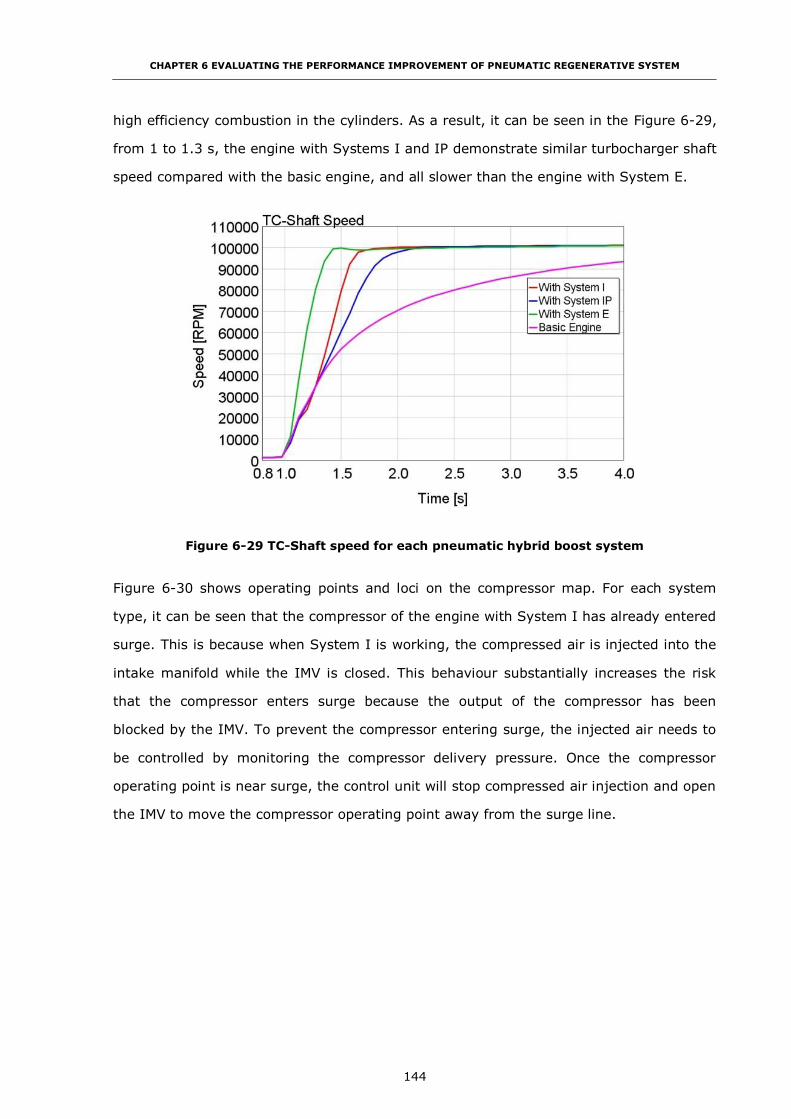
CHAPTER 6 EVALUATING THE PERFORMANCE IMPROVEMENT OF PNEUMATIC REGENERATIVE SYSTEM
144
high efficiency combustion in the cylinders. As a result, it can be seen in the Figure 6-29,
from 1 to 1.3 s, the engine with Systems I and IP demonstrate similar turbocharger shaft
speed compared with the basic engine, and all slower than the engine with System E.
Figure 6-29 TC-Shaft speed for each pneumatic hybrid boost system
Figure 6-30 shows operating points and loci on the compressor map. For each system
type, it can be seen that the compressor of the engine with System I has already entered
surge. This is because when System I is working, the compressed air is injected into the
intake manifold while the IMV is closed. This behaviour substantially increases the risk
that the compressor enters surge because the output of the compressor has been
blocked by the IMV. To prevent the compressor entering surge, the injected air needs to
be controlled by monitoring the compressor delivery pressure. Once the compressor
operating point is near surge, the control unit will stop compressed air injection and open
the IMV to move the compressor operating point away from the surge line.

CHAPTER 6 EVALUATING THE PERFORMANCE IMPROVEMENT OF PNEUMATIC REGENERATIVE SYSTEM
145
Figure 6-30 Turbocharger operation points on compressor efficiency map for each
pneumatic hybrid boost system
Figure 6-30 demonstrates that with System IP there is less chance to cause the
compressor to enter surge. This is because, for System IP, only one intake port is
blocked by the TV during compressed air injection. The compressor still can deliver the
air into the cylinder through another intake port.
From Figure 6-30, System E can be recognized as the safest method to increase the
turbocharger response compared with the Systems I and IP. The injection into the
exhaust manifold accelerates the turbocharger shaft speed, as a result, the compressor’s
output pressure increases rapidly and well away from the surge line.
From the analysis before, it can be seen the engine with System I get the fast brake
torque response and the most air usage. The System IP has the almost the same brake
torque response and air usage. But at the beginning stage, the System IP has the ability
that deliver the compressed air into cylinders as soon as possible. As a result, the engine
with System I and the engine with System IP have been chosen to the candidate to the
vehicle simulation model with pneumatic hybrid boost system. In the next section, the
basic vehicle, the vehicle with System I and the vehicle with System IP model are built in
GT-POWER and their simulation results will be compared.

CHAPTER 6 EVALUATING THE PERFORMANCE IMPROVEMENT OF PNEUMATIC REGENERATIVE SYSTEM
146
6.6 Vehicle with Pneumatic Hybrid Boost System Simulation Result
6.6.1 Vehicle GT-POWER Simulation Models
A 16 ton city bus equipped with the YUCHAI YC6A diesel engine is modelled using the
GT-POWER code with parameters given in Table 6-7.
Table 6-7 City bus parameters
Vehicle weight (kg) 16500
Aerodynamic drag coefficient (-) 0.5
Frontal area (m2) 5.69
Air density (kg/m3) 1.225
Wheel radius (m) 0.508
Rolling resistance coefficient (-) 0.013
Air tank volume (l) 151
Starting tank pressure (bar) 6
1st gear ratio (-) 6.9
2nd gear ratio (-) 4.13
3rd gear ratio (-) 2.45
4th gear ratio (-) 1.49
5th gear ratio (-) 1
Final drive ratio (-) 5.125
The System I and IP respectively have been integrated into the basic bus model giving
two different pneumatic hybrid vehicle configurations. The GT-POWER models of the
basic vehicle, the vehicle with System I and the vehicle with System IP are shown in
Figure 6-31, Figure 6-32 and Figure 6-33 respectively.
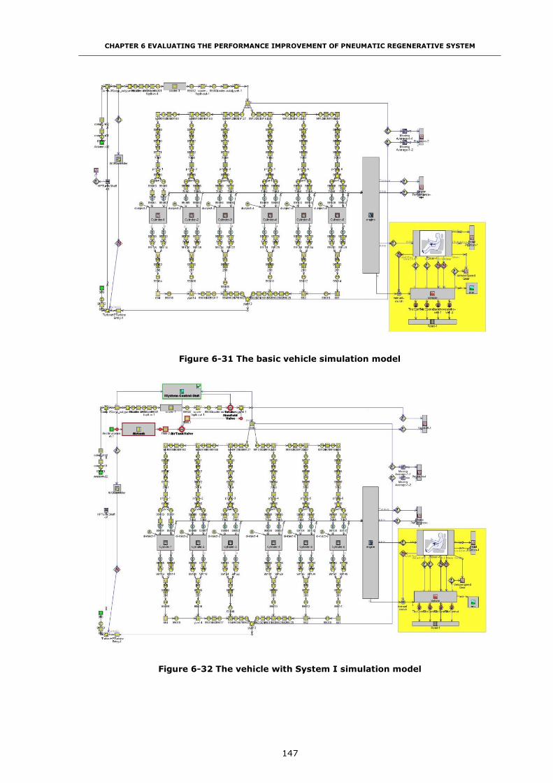
CHAPTER 6 EVALUATING THE PERFORMANCE IMPROVEMENT OF PNEUMATIC REGENERATIVE SYSTEM
147
Figure 6-31 The basic vehicle simulation model
Figure 6-32 The vehicle with System I simulation model

CHAPTER 6 EVALUATING THE PERFORMANCE IMPROVEMENT OF PNEUMATIC REGENERATIVE SYSTEM
148
Figure 6-33 The vehicle with System IP simulation model
6.6.2 Vehicle with Pneumatic Hybrid Boost System Simulation Result
Figure 6-34 Vehicle speed during the acceleration
Figure 6-34 shows the vehicle speed change during the acceleration from 0 to 20 second.
Here, due to GT-POWER setting, when the vehicle start with engine Off, it need some
preparation time to start the engine and then keep the engine speed at the idle speed.

CHAPTER 6 EVALUATING THE PERFORMANCE IMPROVEMENT OF PNEUMATIC REGENERATIVE SYSTEM
149
After that, the vehicle starts to move. As a result, the vehicle is stationary for the first 1
s in Figure 6-34. Then it fully accelerates to the maximum speed. Therefore, a very steep
acceleration at the initial of the test reflects in Figure 6-34. It also can be seen, the
vehicle with System I has the fastest acceleration performance. After 19 s acceleration, it
reaches the speed of 65.3 km/h. The vehicle with System IP has the second fastest
acceleration performance and reaches the speed of 63.5 km/h. The basic vehicle has the
slowest acceleration performance, which reaches the speed of 57 km/h after 19 s
acceleration. Table 6-8 shows the time for three vehicles to reach 48 km/h (30 mph)
which is the speed limit for the most urban city roads in the UK. The Systems I and IP
reduce the acceleration times by 14.7% and 9.7% respectively.
Table 6-8 Time to reach the speed of 48km/h
Time to reach 48km/h
(s)
Improvement
(-)
Basic vehicle 12.9 -
Vehicle with System I 11.0 14.7%
Vehicle with System IP 11.7 9.3%
Figure 6-35 Engine brake torque response during the acceleration
Figure 6-35 shows the engine brake torque during acceleration. From the figure, it can be

CHAPTER 6 EVALUATING THE PERFORMANCE IMPROVEMENT OF PNEUMATIC REGENERATIVE SYSTEM
150
seen, at the beginning stage that the vehicle with the Systems I and IP respectively both
have the greatest capability to build up the brake torque especially in lower gears.
Figure 6-36 shows the air tank pressure drop during the acceleration. From the figure, it
can be seen that System I use 1.02 bar air which is 0.32 bar more than the air usage of
System IP which is 0.69 bar. The difference in air consumption is due to the efficiency of
delivery in System IP. While air is delivered directly to the cylinders, the manifold is
pressured by the slowly accelerating compressor in System I. It also can be learned from
the figure that, the System I and IP activated when the vehicle start and after every gear
change, and the lower gear, the more System I and System IP working time.
Figure 6-36 Air tank pressure drop during the acceleration
From the simulation result, it can be seen that System IP has advantages over System I
at two aspects:
(i) Less use of air to achieve a similar brake torque response,
(ii) Less likely to cause the compressor surge.
6.7 Conclusion
An analysis of the reasons for engine turbo-lag and the methods developed for reducing
the turbo-lag and improving transient response have been presented first. Then, three
kinds of pneumatic hybrid boost systems for managing a rapid energy transfer into the
CHAPTER 6 EVALUATING THE PERFORMANCE IMPROVEMENT OF PNEUMATIC REGENERATIVE SYSTEM
151
powertrain to assist acceleration of the turbocharger, respectively Systems I, IP and E
integrated into a six cylinders 7.25 l heavy-duty diesel engine for a city bus application
have been proposed and investigated from engine brake torque response by using the 1-
D engine simulation. The findings show
(i) The engine with System I has the fastest engine response: 0.25 s to reach its 90%
maximum brake torque, compared with 1.25 s for the basic engine. The System
I, IP and E all improve torque response time (to maximum torque) by 78.3%,
63.5% and 60.9% respectively. The engine with System E has a significantly
lower brake torque output during the first few cycles which reduce the quality of
the engine response.
(ii) The simulation result indicates that System I carries the highest risk of
compressor surge. To avoid surge, a control strategy can be implemented to
ensure the compressor operating point is kelp away from conditions where surge
can develop. System IP carries a lower risk of surge because it does not block
the output of the compressor. Because System E does not need a valve in the
intake system, there is no risk of the surge.
The performance of the vehicle (city bus) has been also considered. A 16 ton city bus
equipped with this engine has been modelled using GT-POWER. The Systems I and IP
have been integrated respectively into the basic bus model. Both the Systems I and IP
can be seen to significantly reduce the vehicle acceleration time through the reduction of
turbo-lag. For the speed range from 0 to 48 km/h (30 mph) which is the speed limit for
most urban roads in the UK, the vehicle with the Systems I and IP can reduce the
acceleration time 13.7% and 9.3% respectively.
System IP offers considerable advantages over System I at both less use of air and less
likely to cause the compressor surge. As a result, System IP should be the appropriate
candidate for the future research such as to develop a pneumatic hybrid system can
achieve three functions: the regenerative braking when decelerating, boosting engine
and eliminating the turbo-lag when accelerating, and the stop-start operation.

CHAPTER 7 DESIGN AND OPTIMIZE THE PNEUMATIC HYBRID CITY BUS CONTROL STRATEGY
152
CHAPTER 7
DESIGN AND OPTIMIZE THE PNEUMATIC HYBRID CITY
BUS CONTROL STRATEGY
7.1 Introduction
After comparing the three principal hybrid vehicle control strategies, respectively rule-
based, global optimisation and real-time optimisation, an energy control strategy based
on the use of thresholds in the degree of energy storage and regeneration (a “logic
threshold” methodology) for the pneumatic hybrid city bus has been designed. By
employing the control strategy, six operation modes of the pneumatic hybrid city bus can
be changed dynamically and the energy distribution of the pneumatic hybrid system can
be controlled to realize the three principal functions of the pneumatic hybrid system,
respectively Stop-Start Function, Boost Function, and Regenerative Braking Function.
A forward facing pneumatic hybrid city bus simulation model which includes the detailed
engine model has been developed in GT-POWER with MATLAB/Simulink co-simulation.
The pneumatic hybrid city bus dynamic performance, engine transient response, fuel
economy and energy usage can be analysed from this model.
To obtain the maximum overall fuel economy, the amount of air and energy recovered
during the braking and minimum loss of availability during acceleration, a number of
variables in the control strategy must be optimized. Three global optimisation algorithms,
Pattern Search (PS), Genetic Algorithm (GA) and multi-objective Non-dominated Sorting
Genetic Algorithm II (NSGA-II), are compared and employed for the optimisation of the
control strategy considered at three levels.
(i) Using the PS to optimize the initial air tank pressure for every stop-start event to
maximize the pressure increment in the air tanks.
(ii) Conducting the GA optimisation to find out the best gear change strategy during
braking to maximize the energy recovery to the air tanks.

CHAPTER 7 DESIGN AND OPTIMIZE THE PNEUMATIC HYBRID CITY BUS CONTROL STRATEGY
153
(iii) Implementing the multi-objective optimisation to simultaneously minimize a) the
fuel consumption and b) the loss of availability in the air flow during a vehicle
acceleration (Using the NSGA-II).
7.2 Pneumatic Hybrid City Bus Control Strategy
Unlike HEVs, the pneumatic hybrid city bus cannot be driven by pneumatic energy alone.
But pneumatic hybrid technology has the potential to be a low-cost alternative to the
electric motor based micro hybrid technology by converting kinetic energy to pneumatic
energy during braking, re-using the stored energy to power an air starter to realize a
stop-start operation. Normally the micro hybrid system is the integration of starter and
alternator in the conventional IC engine vehicle, in which the starter should also function
as an electric motor which tends to add both cost and weight to the vehicle [92]. As
mentioned in Chapter 6, the pneumatic hybrid system also has another advantage which
can improve the engine performance by injecting compressed air into the inlet manifold
to build-up engine torque more rapidly compared with the unassisted engine. So the
pneumatic hybrid city bus control strategy should ensure three functions:
(i) Stop-Start Function: when the vehicle starts, the air starter is cranking the
engine; when the vehicle is stopped, the IC engine is switched off to save the
idle fuel consumption if stop conditions are satisfied.
(ii) Boost Function: during the acceleration, the Boost Function is switched ON to
eliminate the turbo-lag and improve the engine transient response.
(iii) Regenerative Braking Function: During deceleration, the Regenerative Braking
Function is engaged to recover energy.
7.2.1 Overview the Control Strategy of Hybrid Vehicles
The control strategy of a hybrid vehicle is defined as an algorithm which regulates the
operation of the vehicle powertrain [93]. It is usually implemented in the hybrid vehicle
controller which has a supervisory role in regard to the operation of the vehicle. The main
objectives of the hybrid vehicle control strategy are to continuously monitor the driver’s
demand, vehicle status, current traffic information, and even the information provided by
the Global Positioning System (GPS) to determine the proper vehicle operating state for
optimal fuel economy, minimum overall energy use, and vehicle performance [69, 93,

CHAPTER 7 DESIGN AND OPTIMIZE THE PNEUMATIC HYBRID CITY BUS CONTROL STRATEGY
154
94]. Hybrid vehicle control strategies can be divided into three categories: ruled-based,
numerical optimisation-based and real-time optimisation [95]. All the main solutions are
classified according to Figure 7-1.
Figure 7-1 Classification of hybrid vehicle control strategies
7.2.1.1 Rule-based Control Strategies
The rule-based control strategies are designed without a priori knowledge of the driving
cycle. Therefore, they are effective in the real-time supervisory control of the power flow
in the hybrid powertrain. The rules can be obtained by using heuristics, intuition, human
expertise, and even mathematical models [93]. The objective of rule-based control
strategies is often “load-levelling” which tends to shift the actual IC engine operating
point as close as possible to the optimal point of the efficiency, fuel consumption, or
emissions at a particular engine speed. Although the control approaches can offer an
improvement in energy efficiency, it is clear that they do not guarantee an optimal result
in all conditions [95]. Two typical rule-based control strategies are introduced here:
respectively (i) a logic threshold control strategy and (ii) a fuzzy logic control strategy.
The logic threshold control strategy is widely used because of its speed and simplicity
[12]. It based on analysis of power flow in a hybrid powertrain, efficiency/fuel or
emission maps of an IC engine, and human experience is utilized to design deterministic
rules, generally implemented via lookup tables, to split the requested power between
power converters [93]. In other words, the logic threshold control strategy selects the
operating mode of the powertrain according to the prevailing and predicted conditions of
Hybrid vehicle control
strategies
Rule-Based control strategies
Global optimization
Real-time optimization
Logic threshold
control strategy
Fuzzy logic
Dynamic programming
Linear programming
Model predictivecontrol
Equivalent consumption minimization
strategy (ECMS)

CHAPTER 7 DESIGN AND OPTIMIZE THE PNEUMATIC HYBRID CITY BUS CONTROL STRATEGY
155
the vehicle. The transition between operating modes is decided based on a change in
driver demand, or a change in vehicle operating condition.
Looking into the hybrid powertrain as a multi-domain, nonlinear, and time-varying plant,
a fuzzy logic control strategy offers a number of advantages including an accessible
format and the potential for non-linear behaviour [93]. The fuzzy logic control strategy is
an extension of the conventional rule-based control strategy typified by a logic threshold
control strategy [93]. The fuzzy logic control strategy uses the decision-making property
instead of using deterministic rules. As a result, it can be adopted to realize a real-time
though possibly suboptimal power split. The main advantages of the fuzzy logic control
strategy are robustness and the potential for adaptive behaviour [93].
7.2.1.2 Global Optimisation
The global optimisation approach can find the global optimum solution by performing the
optimisation over a prescribed driving cycle. It is non-causal in nature and requires a
priori knowledge of the driving cycle information and could be used directly for real-time
hybrid vehicle control strategy. However, the result of the global optimisation can be
considered as the benchmark for designing rules for online implementation or comparison
for evaluating the quality of other control strategies. The most common global
optimisation approach, Dynamic Programming (DP), is introduced later.
DP seems to be a reasonable approach for optimal power split in hybrid vehicles, since it
is a powerful tool to save general dynamic optimisation problems, easily handling the
constraints and nonlinearity of the problem while obtaining a globally optimal solution
[93]. DP calculates every possible combination energy output of the IC engine and
another power source in the hybrid powertrain such as motor power at each step,
ensuring that the global optimum can be reached. When utilizing DP in the hybrid
powertrain optimisation, the model of hybrid vehicle can be expressed in the form of
Equation (7-1) where XK is the state vector that includes vehicle speed, State of Charge
(SOC) of the energy store, engine speed, motor speed, etc. While uK is the control vector
that covers gear number, generator torque, engine torque, motor torque, etc. The
optimisation goal is to find the control uK at each step to minimize a cost function shown
at Equation (7-2). Also, the constraints in Equation (7-3) are necessary for the
optimisation process.

CHAPTER 7 DESIGN AND OPTIMIZE THE PNEUMATIC HYBRID CITY BUS CONTROL STRATEGY
156
𝑋𝐾+1 = 𝑓(𝑋𝐾, 𝑢𝐾) (7-1) [96]
{𝐽0(𝑋0) = 𝐽0
𝐽𝑘(𝑥𝑘) = min𝑢𝑘∈𝑈𝑘[𝑓𝑢𝑒𝑙(𝑥𝑘, 𝑢𝑘) + 𝐽𝑘−1(𝑥𝑘−1)] 𝑘 = 1, … , 𝑁
(7-2) [96]
{
𝜔𝐼𝐶𝐸 𝑚𝑖𝑛 ≤ 𝜔𝐼𝐶𝐸 ≤ 𝜔𝐼𝐶𝐸 𝑚𝑎𝑥
𝑇𝐼𝐶𝐸 𝑚𝑖𝑛(𝜔𝐼𝐶𝐸(𝑘)) ≤ 𝑇𝐼𝐶𝐸(𝑘) ≤ 𝑇𝐼𝐶𝐸 𝑚𝑎𝑥(𝜔𝐼𝐶𝐸(𝑘))
𝑇𝑚 𝑚𝑖𝑛(𝜔𝑚(𝑘), 𝑆𝑂𝐶(𝑘)) ≤ 𝑇𝑚(𝑘) ≤ 𝑇𝑚 𝑚𝑎𝑥(𝜔𝑚(𝑘), 𝑆𝑂𝐶(𝑘))𝑆𝑂𝐶𝑚𝑖𝑛 ≤ 𝑆𝑂𝐶(𝑘) ≤ 𝑆𝑂𝐶𝑚𝑎𝑥
(7-3) [96]
Where ωICE min – minimum speed of the engine,
ωICE max – maximum speed of the engine,
Tmax – torque limitation of the engine,
Tm min and Tm max – motor torque limitation,
The variable SOC(k) is constrained within the permitted minimum value SOCmin and the
maximum value SOCmax of the battery.
When the energy management strategy is designed, the constraints have to be respected
[97]. For example, in order to mitigate battery degradation, the SOC should be
maintained within a certain range. The torque capacity of the engine and electric motor
vary with their rotational speed or environmental temperature, and the speed of the
engine and electric motor must be limited to the specific range to ensure safety and
reliability [97].
DP will supply a benchmark which can be compared with the rule-based control
strategy’s result. Although the DP can find the global optimum, it is an off-line algorithm.
7.2.1.3 Real-time Optimisation
In order to develop a cost function to be used in a real-time optimisation process, the
rate of fuel consumption must be available as a measurement. Variations of the stored
electrical energy should also be taken into account to guarantee electrical self-
sustainability [93]. Although the solution to such a problem is not globally optimal, it is
particularly suited to real-time implementation and is reported to be close to optimal in
practice [98]. The most well-known approach of the real-time optimisation is the
Equivalent Consumption Minimization Strategy (ECMS).

CHAPTER 7 DESIGN AND OPTIMIZE THE PNEUMATIC HYBRID CITY BUS CONTROL STRATEGY
157
The “equivalent fuel consumption” of the ECMS is the electrical energy flow costed
according how much it will cost in fuel terms to restore that energy to the store.
Application of the ECMS method includes an assessment of the relative value derived
from a drive cycle of electricity and fuel. The process includes the notion of the “free”
energy that is derived from regenerative braking [95]. In [93], one approach, that of
calculating the equivalent fuel consumption using mean efficiencies is used when not all
components set points are known is introduced as follows:
𝐶𝐸𝑞(𝑘(𝑡), 𝑇𝑒(𝑡)) = {𝑇𝑒 < 0
𝑆𝐹𝐶𝑟𝑒𝑐ℎ ∙𝑃𝑐(𝜔𝑐,𝑇𝑐)
𝑐∙𝜂𝑒∙𝜂𝑏𝑎𝑡𝑡
𝑇𝑒 ≥ 0 𝑆𝐹𝐶𝑑𝑖𝑠∙𝑃𝑒(𝜔𝑒,𝑇𝑒)∙𝜂𝑒∙𝜂𝑏𝑎𝑡𝑡
𝑐
(7-4) [93]
where SFCrech – mean specific fuel consumption for the recharge cases,
SFCdis – mean specific fuel consumption for the discharge cases,
𝜂𝑒 – mean efficiencies of the motor during recharge,
𝜂𝑏𝑎𝑡𝑡
– mean efficiencies of the battery during recharge,
c – constant.
The Electric Motor (EM) power to produce Te at ωe is denoted by Pe. And, the total
equivalent fuel consumption CTOT(k(t),Te) is the sum of the real fuel consumption of the
IC engine CICE(k(t),Te) and the equivalent fuel consumption of the EM CEq(k(t),Te). This
allows a unified representation of both the energy used from the battery and the IC
engine respectively. As a result, the instantaneous control problem is
min𝑇𝑒(𝑡),𝑘(𝑡) 𝐽 = 𝐶𝑇𝑂𝑇(𝑘(𝑡), 𝑇𝑒(𝑡)) ∙ Δ (7-5) [93]
Zhao et al. [95] used the idea of the ECMS to realize a real-time optimisation of the fuel
economy of an HEV. The optimisation problem can be explicitly formulated as minimizing
the following cost function in terms of energy:
𝐽𝑓(𝑡𝑓, 𝜇, 𝑆𝑂𝐶) = ∫ �̇�𝑓(𝜏, 𝜇, 𝑥) 𝑑𝜏 + 𝜑(𝑆𝑂𝐶(𝑡0), 𝑆𝑂𝐶(𝑡𝑓))𝑡𝑓
𝑡0 (7-6) [95]
where μ – control variables,
x – engine, motor, and battery states,
SOC(t0) – initial SOC values,

CHAPTER 7 DESIGN AND OPTIMIZE THE PNEUMATIC HYBRID CITY BUS CONTROL STRATEGY
158
SOC(tf) – final SOC values,
𝜑(∙) – penalty function regarding any SOC deviation from its initial value to the final value.
The penalty function is also called the equivalent fuel consumption. For the sake of
optimality, the boundary condition of the terminal state
𝑆𝑂𝐶(𝑡0) = 𝑆𝑂𝐶(𝑡𝑓) (7-7) [95]
is to be satisfied.
Although the ECMS is designed for the HEV, it still can be transferred to control the
pneumatic hybrid vehicles. As mentioned in Chapter 2, some of the pneumatic hybrid
vehicles use the pneumatic energy to drive the vehicle in the AM mode or APA mode. It
means it can save the fuel by using the pneumatic instead of. As a result, the “equivalent
fuel consumption” of the ECMS in the pneumatic hybrid vehicle is the pneumatic energy
flow costed according how much it will cost in fuel terms to restore that energy to the
store. Application of the ECMS method includes an assessment of the relative value
derived from a drive cycle of air and fuel. Furthermore, in the commercial vehicle like
buses and trucks, some auxiliaries are driven by the electricity now. It could be driven by
the air in the future. Therefore, in the pneumatic hybrid vehicles, the fuel used to drive
the auxiliaries can be saved by using the air. As a result, the air usage can be calculated
how much it cost in fuel terms. Here, in this research, the pneumatic hybrid powertrain is
to realize three special functions. It does not drive the vehicle alone by realizing the AM
mode or APA mode. So there is no fuel saved by using the pneumatic energy.
Consequently, there is no energy to be calculated in fuel term. Therefore, the ECMS will
not be chosen for controlling the pneumatic hybrid city bus in this research and not be
discussed in detail.
7.2.2 Logic Threshold Based Energy Control Strategy for Pneumatic
Hybrid City Bus
Compared with other hybrid vehicle control strategies such as DP and ECMS, the logic
threshold based energy control strategy fits for the pneumatic hybrid system requirement
and because it is fast, simple and practical [12].

CHAPTER 7 DESIGN AND OPTIMIZE THE PNEUMATIC HYBRID CITY BUS CONTROL STRATEGY
159
The store of pneumatic energy helps achieve three principal functions. The energy control
strategy for the pneumatic hybrid city bus enables the vehicle to realize the specific
functions mentioned before and summarized below, as well as the normal operation of
the vehicle.
(i) Stop-Start Function: the IC engine is off when the vehicle is stop, to save the
idle fuel consumption if the condition is satisfied; when the vehicle starts, the air
starter is cranking the IC engine.
(ii) Boost Function: during the acceleration, the Boost Function is ON to eliminate
the turbo-lag and improve the engine transient response.
(iii) Regenerative Braking Function: During the deceleration, the Regenerative
Braking Function is ON to recover the energy.
The schematic diagram of the control strategy for the pneumatic hybrid city bus is shown
in Figure 7-2. It can be seen that there are three sub-controllers which are in charge of
realizing the three specific functions above from Figure 7-2. The conditions of the
pneumatic hybrid city bus at each time step form the basis for a decision to transfer the
operating mode or not are also shown in Figure 7-2. In each operating mode, there may
be some sub-states which the vehicle can operate between these states. As the vehicle
enters a new state, the output signals will be implemented to affect the new control state.
The parameters of the logic threshold based energy control strategy for the pneumatic
hybrid city bus are shown in Table 7-1. To obtain the maximum overall fuel economy, the
amount of air and energy recovered during the braking and minimum loss of availability
during acceleration, these variables in the control strategy must be optimized. The goals
and cost function of three optimisations are shown in Figure 7-3.
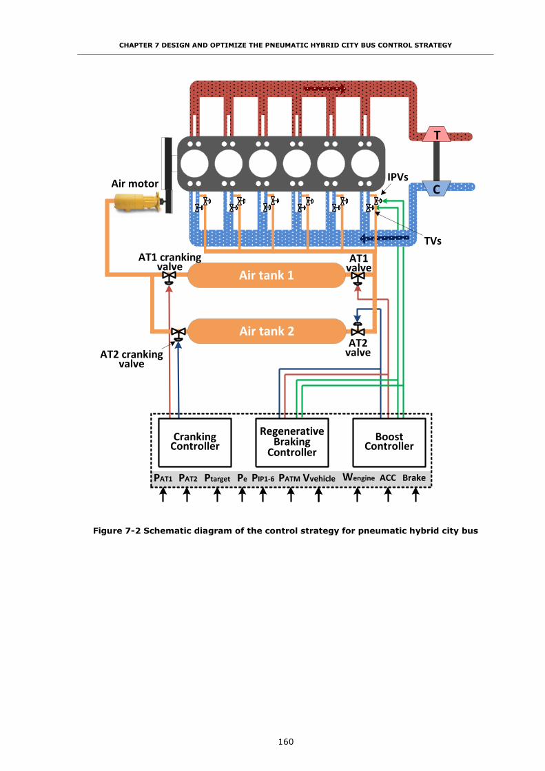
CHAPTER 7 DESIGN AND OPTIMIZE THE PNEUMATIC HYBRID CITY BUS CONTROL STRATEGY
160
Figure 7-2 Schematic diagram of the control strategy for pneumatic hybrid city bus
Air motor
AT1 cranking valve
TVs
IPVsC
T
AT2 cranking valve
AT1 valve
AT2 valve
Air tank 1
Air tank 2
PAT1 PAT2 Pe ACCWengineVvehiclePATM PIP1-6 Ptarget
Cranking Controller
Regenerative Braking
Controller
Boost Controller
Brake

CHAPTER 7 DESIGN AND OPTIMIZE THE PNEUMATIC HYBRID CITY BUS CONTROL STRATEGY
161
Figure 7-3 Schematic diagram of the control strategy optimisation
Co
st
fun
cti
on
of
op
tim
izati
on
Ho
w
PA
T1
PA
T2
Pe
AC
C
Wen
gin
e
Vveh
icle
PA
TM
PIP
1-6
P
targ
et
Brake
Vta
rg
et
Cran
kin
g
Go
al
Cran
kin
g
Co
ntr
oll
er
Sele
ct
air
tan
k
Sta
rt
en
gin
e
AT1
cran
kin
g
valv
e
AT2
cran
kin
g
valv
e
Reg
en
era
tive
Brakin
g
Co
ntr
oll
er
AT1
valv
eA
T2
valv
eTV
s
IP
Vs
Gear c
han
gin
g
str
ate
gy
du
rin
g b
rakin
g
Bo
ost
Co
ntr
oll
er
AT1
valv
e
AT2
valv
e
TV
s
IP
Vs
Gear c
han
gin
g
str
ate
gy
du
rin
g
accele
rati
on
Gear
nu
mb
er
Lo
ok u
p
Tab
le
Sto
p-S
tart
Fu
ncti
on
Reg
en
erati
ve
Brakin
g
Fu
ncti
on
Bo
ost
Fu
ncti
on
Op
tim
ise t
he
init
ial
air
tan
k
pressu
re f
or
every s
top
-sta
rt
even
t
Op
tim
ise t
he
gear c
han
gin
g
str
ate
gy d
urin
g
the a
ccele
rati
on
Op
tim
ise t
he
gear c
han
gin
g
str
ate
gy d
urin
g
the b
rakin
g
Targ
et
To
maxim
ize t
he
tota
l air
tan
k
pressu
re
increm
en
t
To
maxim
ize t
he
tota
l en
erg
y
reco
vered
To
sim
ult
an
eo
usly
m
inim
ize a
) t
he
fuel
co
nsu
mp
tio
n
an
d b
) t
he
red
ucti
on
of
avail
ab
le e
nerg
y
du
e t
o u
se o
f air
fr
om
th
e t
an
ks

CHAPTER 7 DESIGN AND OPTIMIZE THE PNEUMATIC HYBRID CITY BUS CONTROL STRATEGY
162
Table 7-1 Parameters of the logic threshold control strategy for the pneumatic hybrid
city bus
Variables Unit Description
P1 bar The initial pressure of air tank 1
P22 bar The initial pressure of air tank 2
gear12 km/h The gear shift-up point from first to second
gear at vehicle speed
gear23 km/h The gear shift-up point from second to
third gear at vehicle speed
gear34 km/h The gear shift-up point from third to fourth
gear at vehicle speed
gear45 km/h The gear shift-up point from fourth to fifth
gear at vehicle speed
gear21 km/h The gear shift-down point from second to
first gear
gear32 km/h The gear shift-down point from third to
second gear
gear43 km/h The gear shift-down point from fourth to
third gear
gear54 km/h The gear shift-down point from fifth to
fourth gear
The principal fuel economy measure comes from the reduction in the idle time of the
engine because during idle, the engine produces no useful work although it may still be
required to manage the air conditioning and electrical loads. During deceleration or
braking, there is no fuel consumption; recovery of the energy by transferring the kinetic
energy to the pneumatic energy also enhance the system’s energy efficiency through
removing the need for an electrical flow of energy from the engine alternator. The Boost
Function assists the engine in reaching a high efficiency working condition more quickly
than otherwise. These principal functional requirements set the goals for the individual
sub-system control objectives.
The operations modes of the pneumatic hybrid city for a typical driving condition are
explained in Figure 7-4. The figure shows a typical manoeuvre that starts with the engine
off. The engine is started and the vehicle proceeds to accelerate before reaching a steady
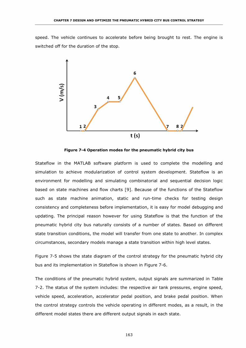
CHAPTER 7 DESIGN AND OPTIMIZE THE PNEUMATIC HYBRID CITY BUS CONTROL STRATEGY
163
speed. The vehicle continues to accelerate before being brought to rest. The engine is
switched off for the duration of the stop.
Figure 7-4 Operation modes for the pneumatic hybrid city bus
Stateflow in the MATLAB software platform is used to complete the modelling and
simulation to achieve modularization of control system development. Stateflow is an
environment for modelling and simulating combinatorial and sequential decision logic
based on state machines and flow charts [9]. Because of the functions of the Stateflow
such as state machine animation, static and run-time checks for testing design
consistency and completeness before implementation, it is easy for model debugging and
updating. The principal reason however for using Stateflow is that the function of the
pneumatic hybrid city bus naturally consists of a number of states. Based on different
state transition conditions, the model will transfer from one state to another. In complex
circumstances, secondary models manage a state transition within high level states.
Figure 7-5 shows the state diagram of the control strategy for the pneumatic hybrid city
bus and its implementation in Stateflow is shown in Figure 7-6.
The conditions of the pneumatic hybrid system, output signals are summarized in Table
7-2. The status of the system includes: the respective air tank pressures, engine speed,
vehicle speed, acceleration, accelerator pedal position, and brake pedal position. When
the control strategy controls the vehicle operating in different modes, as a result, in the
different model states there are different output signals in each state.

CHAPTER 7 DESIGN AND OPTIMIZE THE PNEUMATIC HYBRID CITY BUS CONTROL STRATEGY
164
The control modes which govern the vehicle during this process are now described in
more detail: (Each mode is referred to the Stages shown in Figure 7-4)
(i) Cranking mode (1-2)
In this mode, based on the input signals and the pressure in the two air tanks,
the control strategy assigns one air tank to start the engine by opening the valve
of this air tank. The control strategy for this operation mode is in the sub-
stateflow state Cranking shown in the Figure 7-6.
(ii) Fully acceleration mode (2-3, 5-6)
In the full acceleration mode, the driver demands full (100%) acceleration. The
mode can be either part of an acceleration event like stage 2-3 or a full
acceleration event such as stage 5-6. The control strategy chooses one air tank
to realize the boost function by opening the valves. Based on the finding of
Chapter 3, the lower air tank pressure can recover more braking energy during
the deceleration. As a result, the control strategy chooses the air tank with lower
pressure to implement the boost function. In the Stateflow representation of this
control strategy, in the state Acceleration, the states AT1Boost and AT2Boost
compose this operation mode.
(iii) Acceleration mode (3-4)
Acceleration mode is selected when the driver demand is less than 100%.
Referring to Figure 7-6 there is a sub-state BoostOff in the state Acceleration.
BoostOff defines the acceleration mode. The vehicle operation modes can
transfer between these two modes depending on the driver demand.
(iv) Cruise mode (4-5)
In this mode, the vehicle has a fixed speed.
(v) Deceleration mode (6-7)
The deceleration mode is the Brake state in the Figure 7-6. Based on the
pneumatic hybrid system condition, the control strategy controls the vehicle to
operate between three states:
a) Regeneration to air tank 1 (RegenerativeBrakingOnAT1RecoveryAir = TRUE)
b) Regeneration to air tank 2 (RegenerativeBrakingOnAT2RecoveryAir = TRUE)
c) Regeneration off (RegenerativeBrakingOff = TRUE)
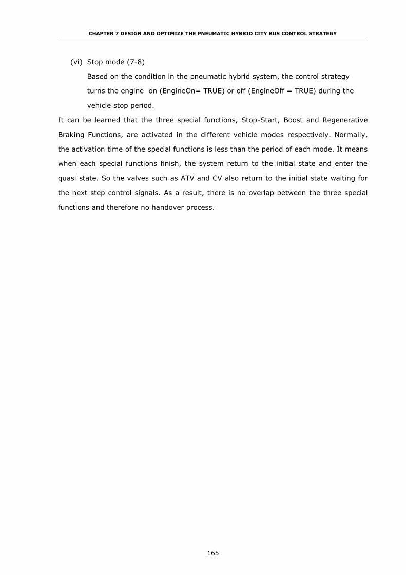
CHAPTER 7 DESIGN AND OPTIMIZE THE PNEUMATIC HYBRID CITY BUS CONTROL STRATEGY
165
(vi) Stop mode (7-8)
Based on the condition in the pneumatic hybrid system, the control strategy
turns the engine on (EngineOn= TRUE) or off (EngineOff = TRUE) during the
vehicle stop period.
It can be learned that the three special functions, Stop-Start, Boost and Regenerative
Braking Functions, are activated in the different vehicle modes respectively. Normally,
the activation time of the special functions is less than the period of each mode. It means
when each special functions finish, the system return to the initial state and enter the
quasi state. So the valves such as ATV and CV also return to the initial state waiting for
the next step control signals. As a result, there is no overlap between the three special
functions and therefore no handover process.

CHAPTER 7 DESIGN AND OPTIMIZE THE PNEUMATIC HYBRID CITY BUS CONTROL STRATEGY
166
Figure 7-5 State diagram of control strategy for the pneumatic hybrid city bus
Sto
p
En
gin
eO
n
Sta
rt
En
gin
eO
ff
Acc
ele
rati
on
AT
1B
oo
st
Bo
ostO
ff
AT
2B
oo
st
Cru
ise
Bra
ke
Reg
en
era
tiv
e
Bra
kin
gO
nA
T
1R
ec
ove
ryA
ir
Reg
en
era
tiv
e
Bra
kin
gO
nA
T
2R
ec
ove
ryA
ir
Reg
en
era
tiv
e
Bra
kin
gO
ff
Cra
nkin
g
No
Cra
nkin
g
AT
1C
ran
kin
gA
T2
Cra
nkin
g
En
gin
eO
ff=
0E
ng
ineO
ff=
1
En
gin
eO
ff=
0
En
gin
eO
ff=
1
V>
=0
&
dV
>=
0
V>
=0
&
dV
=0
V>
=0
&
dV
<0
V=
0
& d
V=
0
V>
=0
&
dV
>0
V>
=0
&
dV
=0
V>
=0
&
dV
>0
AT
1=
1
& B
oo
st=
1
AT
1=
0o
r B
oo
st=
0
AT
1=
1&
Bo
ost=
1
Bo
ost=
0
AT
2=
1&
Bo
ost=
1 AT
2=
0o
r B
oo
st=
0
AT
2=
1&
Bo
ost=
1
AT
1=
1
& R
eg
en
=1
AT
2=
1
& R
eg
en
=1
Reg
en
=0
AT
1=
1
& R
eg
en
=1
AT
2=
1
& R
eg
en
=1
AT
1=
0
or
Re
gen
=0
AT
2=
0
or
Re
gen
=0
V>
=0
&
dV
<0
Cra
nkin
g=
0
Cra
nkin
g=
1
& A
T1
Cra
nkin
g=
1C
ran
kin
g=
1
& A
T2C
ran
kin
g=
1
Cra
nkin
g=
1
& A
T1
Cra
nkin
g=
1
Cra
nkin
g=
1
& A
T2
Cra
nkin
g=
1
Cra
nkin
g=
0C
ran
kin
g=
0

CHAPTER 7 DESIGN AND OPTIMIZE THE PNEUMATIC HYBRID CITY BUS CONTROL STRATEGY
167
Figure 7-6 Stateflow diagram of control strategy for the pneumatic hybrid city bus
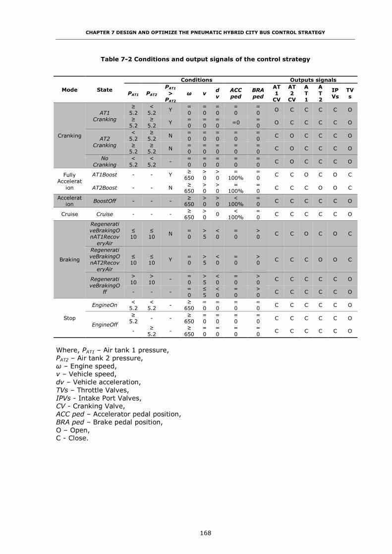
CHAPTER 7 DESIGN AND OPTIMIZE THE PNEUMATIC HYBRID CITY BUS CONTROL STRATEGY
168
Table 7-2 Conditions and output signals of the control strategy
Mode State
Conditions Outputs signals
PAT1 PAT2
PAT1
> PAT2
ω v d
v
ACC
ped
BRA
ped
AT
1 CV
AT
2 CV
A
T1
A
T 2
IP
Vs
TV
s
Cranking
AT1
Cranking
≥
5.2
<
5.2 Y
=
0
=
0
=
0
=
0
=
0 O C C C C O
≥ 5.2
≥ 5.2
Y = 0
=0
=0
=0 = 0
O C C C C O
AT2
Cranking
<
5.2
≥
5.2 N
=
0
=
0
=
0
=
0
=
0 C O C C C O
≥ 5.2
≥ 5.2
N = 0
=0
=0
= 0
= 0
C O C C C O
No
Cranking
<
5.2
<
5.2 -
=
0
=
0
=
0
=
0
=
0 C O C C C O
Fully Accelerat
ion
AT1Boost - - Y ≥
650
>
0
>
0
=
100%
=
0 C C O C O C
AT2Boost - - N ≥
650 >0
>0
= 100%
= 0
C C C O O C
Acceleration
BoostOff - - - ≥
650 >0
>0
< 100%
= 0
C C C C C O
Cruise Cruise - - - ≥
650
>
0 0
<
100%
=
0 C C C C C O
Braking
Regenerati
veBrakingOnAT1Recov
eryAir
≤ 10
≤ 10
N = 0
>5
<0
= 0
> 0
C C O C O C
Regenerati
veBrakingOnAT2Recov
eryAir
≤ 10
≤ 10
Y = 0
>5
<0
= 0
> 0
C C C O O C
Regenerati
veBrakingOff
>
10
>
10 -
=
0
>
5
<
0
=
0
>
0 C C C C C O
- - - =
0
≤
5
<
0
=
0
>
0 C C C C C O
Stop
EngineOn <
5.2 <
5.2 -
≥ 650
=0
=0
= 0
= 0
C C C C C O
EngineOff
≥ 5.2
- - ≥
650 =0
=0
= 0
= 0
C C C C C O
- ≥
5.2 -
≥ 650
=0
=0
= 0
= 0
C C C C C O
Where, PAT1 – Air tank 1 pressure,
PAT2 – Air tank 2 pressure,
ω – Engine speed, v – Vehicle speed,
dv – Vehicle acceleration,
TVs – Throttle Valves,
IPVs - Intake Port Valves, CV - Cranking Valve,
ACC ped – Accelerator pedal position,
BRA ped – Brake pedal position,
O – Open, C - Close.

CHAPTER 7 DESIGN AND OPTIMIZE THE PNEUMATIC HYBRID CITY BUS CONTROL STRATEGY
169
7.3 Pneumatic Hybrid City Bus Simulation Model
The vehicle simulation model has been built in the GT-POWER and MATLAB/Simulink.
Figure 7-7 shows the GT-POWER model, and Figure 7-8 shows the MATLAB/Simulink
model. The connections between these two models are the part
PneumaticHybridVehicle_Controller_Simulink, highlighted in blue in Figure 7-7, and part
GT-SUITE Model1, highlighted in red in Figure 7-8. The part
PneumaticHybridVehicle_Controller_Simulink belongs to the ‘SimulinkHarness’ template
in the GT-POWER. Its function is to couple GT-POWER to MATLAB/Simulink and to enable
the co-simulation process. This is a common practice in the industry where the engine,
powertrain, and vehicle physics are modelled in GT-POWER, and electronic controllers are
modelled in Simulink [99]. How to run the GT-POWER and Simulink co-simulation is
introduced in Appendix-II in detail.
Figure 7-7 The pneumatic hybrid city bus GT-POWER part simulation model
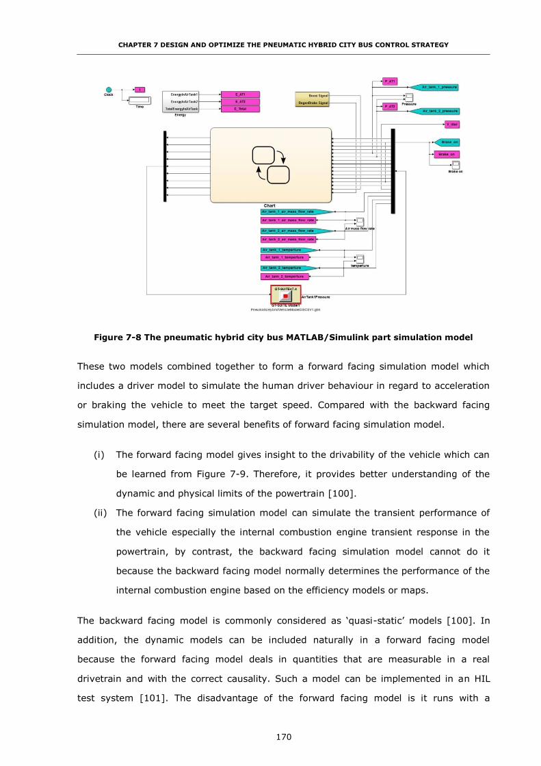
CHAPTER 7 DESIGN AND OPTIMIZE THE PNEUMATIC HYBRID CITY BUS CONTROL STRATEGY
170
Figure 7-8 The pneumatic hybrid city bus MATLAB/Simulink part simulation model
These two models combined together to form a forward facing simulation model which
includes a driver model to simulate the human driver behaviour in regard to acceleration
or braking the vehicle to meet the target speed. Compared with the backward facing
simulation model, there are several benefits of forward facing simulation model.
(i) The forward facing model gives insight to the drivability of the vehicle which can
be learned from Figure 7-9. Therefore, it provides better understanding of the
dynamic and physical limits of the powertrain [100].
(ii) The forward facing simulation model can simulate the transient performance of
the vehicle especially the internal combustion engine transient response in the
powertrain, by contrast, the backward facing simulation model cannot do it
because the backward facing model normally determines the performance of the
internal combustion engine based on the efficiency models or maps.
The backward facing model is commonly considered as ‘quasi-static’ models [100]. In
addition, the dynamic models can be included naturally in a forward facing model
because the forward facing model deals in quantities that are measurable in a real
drivetrain and with the correct causality. Such a model can be implemented in an HIL
test system [101]. The disadvantage of the forward facing model is it runs with a

CHAPTER 7 DESIGN AND OPTIMIZE THE PNEUMATIC HYBRID CITY BUS CONTROL STRATEGY
171
relatively smaller time step when compared to the backward facing model, resulting in
very much longer simulation time. For example, most time step value for continuous
simulation in the GT-POWER is 0.001 s [90].
Figure 7-9 Forward facing hybrid vehicle model
In this research, the forward facing model is utilised for the purpose of vehicle control
strategy optimisation in order to produce more precise results than would be produced by
a backward facing model [102].
7.3.1 Engine and Pneumatic Regenerative System Model

CHAPTER 7 DESIGN AND OPTIMIZE THE PNEUMATIC HYBRID CITY BUS CONTROL STRATEGY
172
Figure 7-10 Engine and pneumatic regenerative system model in GT-POWER
The engine and pneumatic regenerative system model are shown in Figure 7-10, where
the parts of the pneumatic regenerative system are highlighted in red which includes two
air tanks, pipes, valves and the simulated air starter. This model using here is developed
from the pneumatic hybrid engine concept mentioned in Chapter 1 and two air tanks
pneumatic hybrid engine backward facing model in Chapter 4. It is based on the engine
with System IP model using in Chapter 6 and with an added air tank. It has the same
parameters of the pneumatic regenerative system and the engine main technical
parameters are summarized in Table 7-3.
Table 7-3 Main technical parameters of the engine and pneumatic regenerative system
Displacement (l) 7.25
Electronic control system High pressure & common rail
No. of Cylinders (-) 6
Bore (mm) 108
Stroke (mm) 132
Compression ratio (-) 17.5:1
Intake way Turbo-charging & inter-cooling
Rated power/speed (kW/rpm) 177/2300
Max. torque/speed (Nm/rpm) 900/1400~1600
Intake valve (-) 2
Diameter (mm) 32.5
Opening point (normal) 61°BTDC
Closing point (normal) 91°ABDC
Exhaust valve (-) 2
Diameter (mm) 29.5
Opening point (normal) 105°BBDC
Closing point (normal) 67°ATDC
Air tank volume (l) 151
No. of Air tank (-) 2

CHAPTER 7 DESIGN AND OPTIMIZE THE PNEUMATIC HYBRID CITY BUS CONTROL STRATEGY
173
The GT-POWER model also includes a ‘DIWiebe’ combustion sub model and a ‘WoschniGT’
heat transfer sub model used also in Chapter 6. These two sub models are introduced in
Appendix-III in detailed.
7.3.2 Vehicle Model
In this research, the main objective is to study the relationship between the vehicle
performance, the engine fuel consumption and the pneumatic hybrid powertrain energy
recovery efficiency. The schematic representation of the forces acting on the city bus is
presented in Figure 7-11.
Figure 7-11 Forces acting on the city bus
The elementary equation that describes the longitudinal dynamics of a road vehicle has
the follow equation.
𝑀𝑑
𝑑𝑡𝑣 = 𝐹𝑡 − (𝐹𝑤 + 𝐹𝑟 + 𝐹𝑔) (7-8)
where Fw – aerodynamic friction,
Fr – rolling friction,
Fg – force caused by gravity when driving on non-horizontal roads,
Ft – traction force,
M – vehicle mass,
v – vehicle speed.
The aerodynamic friction Fw can be expressed through Equation (7-9).
𝐹𝑤 =1
2𝜌𝑎𝐴𝑓𝑐𝑑𝑣2 (7-9)

CHAPTER 7 DESIGN AND OPTIMIZE THE PNEUMATIC HYBRID CITY BUS CONTROL STRATEGY
174
where v – vehicle speed,
ρa – density of the ambient air,
cd – aerodynamic drag coefficient,
Af – frontal area of the vehicle.
The rolling friction Fr is modelled as
𝐹𝑟 = 𝐹𝑟𝑓 + 𝐹𝑟𝑟 = 𝑐𝑟𝑀𝑔 cos 𝛼 (7-10)
where M – vehicle mass,
g – acceleration due to gravity and
cr – coefficient of the rolling resistance.
Frf – rolling friction on the front axle,
Frr – rolling friction on the rear axle.
The term cosα models the influence of a non-horizontal road. For this research, only the
horizontal road is considered, as a result, α is 0.
The uphill driving force Fg is modelled by the relationship
𝐹𝑔 = 𝑀𝑔 sin 𝛼 (7-11)
The normal load on the front axle Wf can be determined as
𝑊𝑓 =𝑏
𝐿𝑀𝑔 cos 𝛼 − ℎ𝑔(𝐹𝑡 − 𝐹𝑟(1 −
𝑟𝑑
ℎ𝑔)) (7-12) [6]
Similarly, the normal load acting on the rear axle Wr can be expressed as
𝑊𝑟 =𝑎
𝐿𝑀𝑔 cos 𝛼 + ℎ𝑔(𝐹𝑡 − 𝐹𝑟(1 −
𝑟𝑑
ℎ𝑔)) (7-13) [6]
where rd – effective radius of the wheel,
hg – gravity centre height of the vehicle,
a – distance from gravity centre to front wheel centre,
b – distance from the gravity centre to front wheel centre,
L – wheelbase.
From the Equation (7-14), the traction force Ft for a rear-wheel-drive vehicle can be
expressed as

CHAPTER 7 DESIGN AND OPTIMIZE THE PNEUMATIC HYBRID CITY BUS CONTROL STRATEGY
175
𝐹𝑡 =𝜇𝑀𝑔 cos 𝛼[𝐿−𝐶𝑟(ℎ𝑔−𝑟𝑑)]/𝐿
1−𝜇ℎ𝑔/𝐿 (7-14)
where μ – the friction coefficient.
The kinetic energy of the vehicle can be calculated by the following equation
𝐸 =1
2𝑀Δ𝑣2 (7-15)
where, Δv – the speed decrement from regenerative braking start to end during the
braking.
Equation (7-15) indicates that the maximum kinetic energy can be recovered during the
braking. But in the real practice, because of the friction loss, only a percentage of the
initial kinetic energy of the car can be recovered.
Figure 7-12 Vehicle subsystem model in GT-POWER
The vehicle model is composed of the Vehicle2WD-1 part and the tyre model which are in
the orange background shown in the Figure 7-7. The vehicle model Vehicle2WD-1 is
highlighted in green in the Figure 7-7 which is a Vehicle2WD template in the GT-POWER.
It is a compound part which encapsulates a 2-wheel drive vehicle and its drivetrain

CHAPTER 7 DESIGN AND OPTIMIZE THE PNEUMATIC HYBRID CITY BUS CONTROL STRATEGY
176
together which may be connected to an appropriate engine model through a clutch or
torque converter. Its subsystem configuration is shown in the Figure 7-12.
The subsystem includes the transmission model, vehicle model, driveshaft model, and
brake model. Their functions are summarized in Table 7-4.
Table 7-4 Summary the function of the parts in the vehicle subsystem
Part name Function
Transmission Set the gear number, gear ratio, gear transition time, friction mechanical
efficiency and inertia.
Driveshaft Set the shaft moment of inertia and friction mechanical efficiency.
CAR
Set vehicle mass, fuel density, vehicle drag coefficient, vehicle lift
coefficient, vehicle frontal area, centre of pressure, vehicle wheelbase
and mass centre position.
Brake Define the braking torque model map beads on the brake actuator
position.
The Vehicle2WD-1 transmits a vehicle load (including vehicle's inertia load) back to the
engine model as a torque. The speed of the engine and the vehicle drivetrain (which are
geared together by the transmission) is then calculated by the engine model. This speed
is calculated taking the engine's brake torque and subtracting from it the load torque
applied by the vehicle (as well as any auxiliary torque applied to the engine model), and
then using any remaining "positive" torque to accelerate the powertrain. As a result, the
simulation includes the transient response of the engine facilitating the investigation of
the control of both the engine and its subsystems.
7.3.3 Driver Model
The driver model, Driver-1 is highlighted in red in Figure 7-7. Its function is used to
represent the driver who controls accelerator position, brake pedal position, transmission
gear number, clutch pedal position. It is primarily used for controlling vehicles with
manual transmissions as it contains the necessary functions for vehicle launch
(driveaway event) and gear shifting. The input and output of the driver model are shown
in the Figure 7-13.

CHAPTER 7 DESIGN AND OPTIMIZE THE PNEUMATIC HYBRID CITY BUS CONTROL STRATEGY
177
Figure 7-13 Input and output of the driver model
7.3.4 Driving Cycles Model
The Driving Cycles model is highlighted in yellow in Figure 7-7. It is a signal generator
template in the GT-POWER. The generated signal may be generated via several options,
including constant, equation, or imposed time series. This template can also be used to
generate a signal of the current time, angle, or cycle at each time step.
7.3.5 Air Tanks Energy Recovery Model
In order to evaluate the energy recovery efficiency, a twin air tank energy recovery sub
model has been implemented in MATLAB/Simulink, Energy and is shown in Figure 7-8. Its
diagram is shown in Figure 7-14.
Figure 7-14 Air tanks energy recovery model in MATLAB/Simulink
The air tank has been modelled as a control volume, which exchanges air mass only with
the pipes connecting the air tank. The air tanks have a fixed volume VAT. It is assumed

CHAPTER 7 DESIGN AND OPTIMIZE THE PNEUMATIC HYBRID CITY BUS CONTROL STRATEGY
178
that the air tank is well insulated so that there is no heat transfer between the air tanks
and the environment. The mean-value model of the air tank state is calculated using the
following Equations, (7-16 and 7-17)
𝑝𝑣𝐴𝑇 = 𝑚𝑅𝑇 (7-16)
where p – air tank pressure,
m – air mass in the air tank,
R – gas constant,
T – air tank pressure.
Δ𝐸 = Δ𝑚𝑐𝑣𝑇0 (7-17)
where ΔE – energy increment in the air tank,
Δm – air mass increment in the air tank,
cv – volumetric heat capacity of the air,
T0 – start temperature in the air tank.
The Equation (7-17) is based on the first law of the thermodynamics. It cannot point out
the maximum amount of energy that can be extracted from an energy system. The
useful work potential of an energy system at the specified state is called “availability”
(also called “exergy”) [103]. It is based on the second law of thermodynamics and is the
basis for evaluating the capacity of work production in an open, steady flow system or a
closed system. Availability is a measure of the maximum work produced by an energy
system and it depends on the states of the energy system. The availability of air stored
in the air tank is described by the following Equation (7-18). During the acceleration, the
boost function is activated, the air flows out the air tank to be injected into the cylinders.
Compare with calculating the energy decrement of the air tank, the calculation of
availability can present the amount of useful work has been transferred to realize the
boost function. The calculation of availability is introduced in Appendix-IV in detail.
Δ𝐴 = 𝑚𝑅𝑇0(ln𝑝0
𝑝1+
𝑝1
𝑝0− 1) (7-18)
where Δ𝐴 – total availability change in the air tank,
𝑚 – air mass increment in the air tank,
p1 – initial pressure of the air tank,
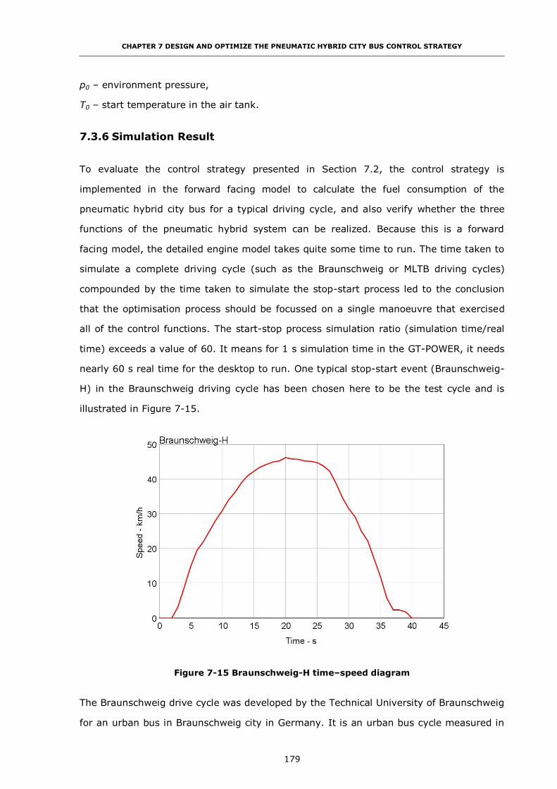
CHAPTER 7 DESIGN AND OPTIMIZE THE PNEUMATIC HYBRID CITY BUS CONTROL STRATEGY
179
p0 – environment pressure,
T0 – start temperature in the air tank.
7.3.6 Simulation Result
To evaluate the control strategy presented in Section 7.2, the control strategy is
implemented in the forward facing model to calculate the fuel consumption of the
pneumatic hybrid city bus for a typical driving cycle, and also verify whether the three
functions of the pneumatic hybrid system can be realized. Because this is a forward
facing model, the detailed engine model takes quite some time to run. The time taken to
simulate a complete driving cycle (such as the Braunschweig or MLTB driving cycles)
compounded by the time taken to simulate the stop-start process led to the conclusion
that the optimisation process should be focussed on a single manoeuvre that exercised
all of the control functions. The start-stop process simulation ratio (simulation time/real
time) exceeds a value of 60. It means for 1 s simulation time in the GT-POWER, it needs
nearly 60 s real time for the desktop to run. One typical stop-start event (Braunschweig-
H) in the Braunschweig driving cycle has been chosen here to be the test cycle and is
illustrated in Figure 7-15.
Figure 7-15 Braunschweig-H time–speed diagram
The Braunschweig drive cycle was developed by the Technical University of Braunschweig
for an urban bus in Braunschweig city in Germany. It is an urban bus cycle measured in
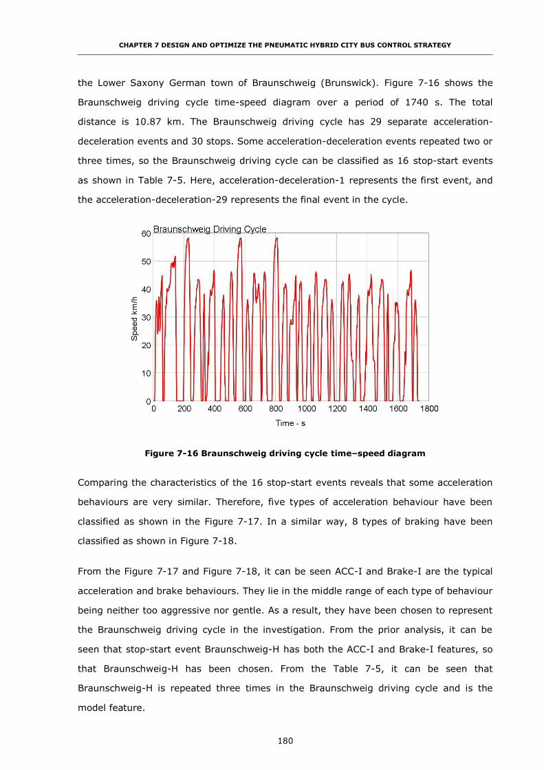
CHAPTER 7 DESIGN AND OPTIMIZE THE PNEUMATIC HYBRID CITY BUS CONTROL STRATEGY
180
the Lower Saxony German town of Braunschweig (Brunswick). Figure 7-16 shows the
Braunschweig driving cycle time-speed diagram over a period of 1740 s. The total
distance is 10.87 km. The Braunschweig driving cycle has 29 separate acceleration-
deceleration events and 30 stops. Some acceleration-deceleration events repeated two or
three times, so the Braunschweig driving cycle can be classified as 16 stop-start events
as shown in Table 7-5. Here, acceleration-deceleration-1 represents the first event, and
the acceleration-deceleration-29 represents the final event in the cycle.
Figure 7-16 Braunschweig driving cycle time–speed diagram
Comparing the characteristics of the 16 stop-start events reveals that some acceleration
behaviours are very similar. Therefore, five types of acceleration behaviour have been
classified as shown in the Figure 7-17. In a similar way, 8 types of braking have been
classified as shown in Figure 7-18.
From the Figure 7-17 and Figure 7-18, it can be seen ACC-I and Brake-I are the typical
acceleration and brake behaviours. They lie in the middle range of each type of behaviour
being neither too aggressive nor gentle. As a result, they have been chosen to represent
the Braunschweig driving cycle in the investigation. From the prior analysis, it can be
seen that stop-start event Braunschweig-H has both the ACC-I and Brake-I features, so
that Braunschweig-H has been chosen. From the Table 7-5, it can be seen that
Braunschweig-H is repeated three times in the Braunschweig driving cycle and is the
model feature.
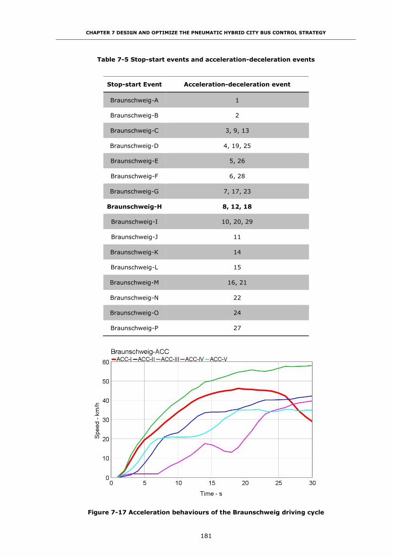
CHAPTER 7 DESIGN AND OPTIMIZE THE PNEUMATIC HYBRID CITY BUS CONTROL STRATEGY
181
Table 7-5 Stop-start events and acceleration-deceleration events
Stop-start Event Acceleration-deceleration event
Braunschweig-A 1
Braunschweig-B 2
Braunschweig-C 3, 9, 13
Braunschweig-D 4, 19, 25
Braunschweig-E 5, 26
Braunschweig-F 6, 28
Braunschweig-G 7, 17, 23
Braunschweig-H 8, 12, 18
Braunschweig-I 10, 20, 29
Braunschweig-J 11
Braunschweig-K 14
Braunschweig-L 15
Braunschweig-M 16, 21
Braunschweig-N 22
Braunschweig-O 24
Braunschweig-P 27
Figure 7-17 Acceleration behaviours of the Braunschweig driving cycle
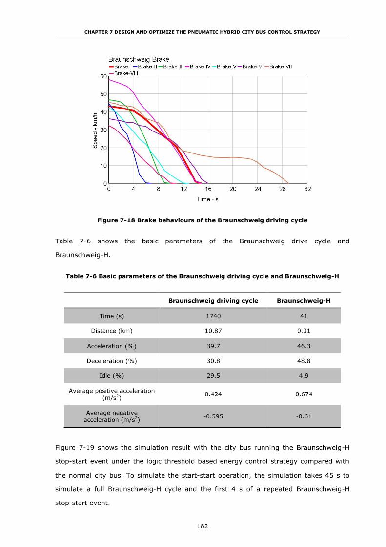
CHAPTER 7 DESIGN AND OPTIMIZE THE PNEUMATIC HYBRID CITY BUS CONTROL STRATEGY
182
Figure 7-18 Brake behaviours of the Braunschweig driving cycle
Table 7-6 shows the basic parameters of the Braunschweig drive cycle and
Braunschweig-H.
Table 7-6 Basic parameters of the Braunschweig driving cycle and Braunschweig-H
Braunschweig driving cycle Braunschweig-H
Time (s) 1740 41
Distance (km) 10.87 0.31
Acceleration (%) 39.7 46.3
Deceleration (%) 30.8 48.8
Idle (%) 29.5 4.9
Average positive acceleration
(m/s2) 0.424 0.674
Average negative
acceleration (m/s2) -0.595 -0.61
Figure 7-19 shows the simulation result with the city bus running the Braunschweig-H
stop-start event under the logic threshold based energy control strategy compared with
the normal city bus. To simulate the start-start operation, the simulation takes 45 s to
simulate a full Braunschweig-H cycle and the first 4 s of a repeated Braunschweig-H
stop-start event.

CHAPTER 7 DESIGN AND OPTIMIZE THE PNEUMATIC HYBRID CITY BUS CONTROL STRATEGY
183
Figure 7-19 Simulation results of the control strategy of the pneumatic hybrid city bus
comparing with the normal city bus
From Figure 7-19, it can be seen that the three functions of the pneumatic hybrid system
have all been realized. In the Speed diagram (a), both the pneumatic hybrid city bus and
the normal city bus can be seen to follow the target driving cycle speed especially in the
acceleration event. The Root Mean Square Error (RMSE) of the normal city bus and
pneumatic hybrid city bus to the target driving cycle speed are summarized in Table 7-7.

CHAPTER 7 DESIGN AND OPTIMIZE THE PNEUMATIC HYBRID CITY BUS CONTROL STRATEGY
184
Table 7-7 RMSE of normal city bus and pneumatic hybrid city bus to the target driving
cycle speed
RMSE –
Acceleration
(3 to 20 s)
RMSE –
Deceleration
(21 to 42 s)
RMSE –
Total
(0 to 45 s)
Normal city bus 0.512 2.889 2.941
Pneumatic hybrid city bus 0.338 2.618 2.642
From the Torque diagram (b) and Engine Speed (c) diagram, it can be seen that in the
two stop periods, the engine is stopped in order to eliminate the idle fuel consumption. In
these two periods, the engine consumes no fuel while in the conventional implementation,
the engine load and speed are respectively 56 Nm and 650 rpm, the normal idle
condition, which represents a significant fuel consumption. It means the Boost Function
has been achieved.
For the Boost Function, it can be seen from the Torque diagram (b) that in the first few
seconds of the first start, the hybrid bus develops torque output more quickly compared
with the normal city bus.
The Regenerative Braking Function also can be verified from the Torque diagram (c).
During the braking period, the engine in the hybrid bus shows a larger brake torque than
the normal city bus. This demonstrates that during the braking process the additional
work done on the bus comes from the additional braking function of the engine and
notably the pumping of air into the respective air tanks.
The Boost Function can be seen in detail in Figure 7-20 and Figure 7-21 respectively. In
the first 10 s, the control strategy implements the Boost Function twice. The first
happens just after the clutch finishes the engaging operation between 3 to 4 s. The Boost
Function increases the air supply to the cylinder to reduce the turbo-lag and improve the
engine transient response. The hybrid city bus demonstrates a faster increase in engine
brake torque output with a lower fuel consumption. The reason for this is during the
boost period, the increased air supply improves the quality of combustion. The engine
operation point has been moved to the high efficiency area faster. For the normal engine,
more time is needed because the turbocharger cannot build the required pressure in the

CHAPTER 7 DESIGN AND OPTIMIZE THE PNEUMATIC HYBRID CITY BUS CONTROL STRATEGY
185
intake manifold sufficiently quickly. This also proves that the pneumatic hybrid
technology not only can improve fuel consumption by realizing the Stop-Start Function,
but also by implementing the Boost Function to improve the engine transient
performance and efficiency.
Figure 7-20 Brake torque for the first 10 s
Figure 7-21 Brake specific fuel consumption for the first 10 s

CHAPTER 7 DESIGN AND OPTIMIZE THE PNEUMATIC HYBRID CITY BUS CONTROL STRATEGY
186
Figure 7-22 shows the average fuel consumption difference between the pneumatic
hybrid city bus and the normal city bus during the Braunschweig-H from 0 to 41 s. Due
to the Boost Function, the pneumatic hybrid city bus has lower average fuel consumption
which is 47.674 l/100km compared with 48.15 l/100km of the normal city bus. The fuel
consumption can be further improved 0.8% by implementing the Boost Function as far of
the already proved ability to reduce fuel consumption by at least 6% by realizing the
stop-start operation (see Chapter 4). Although this improvement of the fuel consumption
is small, it has no practical doubt because it is really a critical change. Firstly, from the
Figure 7-20 and Figure 7-21 with the previous analysis, it can be learned that from the
theoretical analysis and simulation result, the Boost Function improves the quality of
combustion. As a result, it should reduce the transient fuel consumption. Second,
although this 0.8% result is from the simulation result, it still can be trusted, because the
1-D solver of the simulation code, GT-POWER, is considered accurate and convictive [90].
The result can reflect the difference between the normal vehicles and the pneumatic
hybrid vehicles. Finally, this 0.8% improvement in fuel consumption is only in a 42 s
driving cycle. And furthermore, the Boost Function is only activated for very short periods
during the acceleration. Therefore, if using it in the whole Braunschweig driving cycle,
the Boost Function of the pneumatic hybrid city bus can save more fuel.
Figure 7-22 Average fuel consumption during the Braunschweig-H

CHAPTER 7 DESIGN AND OPTIMIZE THE PNEUMATIC HYBRID CITY BUS CONTROL STRATEGY
187
Figure 7-23 and Figure 7-24 show how the Regenerative Braking Function has been
achieved by the control strategy. From Figure 7-23, it can be seen that the pneumatic
hybrid city bus shows the less energy dissipation during the braking because the kinetic
energy of the vehicle has been transferred to the pneumatic energy stored in the air tank.
This can be seen in Figure 7-24. During braking, the control strategy controls the air tank
2 to recover the energy. The pressure of air tank 2 increases from 2.92 bar to 5.25 bar.
Figure 7-23 Total energy dissipated during the braking
Figure 7-24 Air tanks pressure during the Braunschweig-H

CHAPTER 7 DESIGN AND OPTIMIZE THE PNEUMATIC HYBRID CITY BUS CONTROL STRATEGY
188
From Figure 7-24, it can be seen that when the vehicle starts, air tank 1 has been chosen
to supply the air starter, which results in a pressure drop of 0.48 bar. Later, when boost
is required, the control strategy selects the Boost Function, Between 3 s and 10 s, the
engine has been boosted twice which consumes 0.15 bar and 0.05 bar respectively. For
the second engine start operation, because the air tank 2 has the higher air tank
pressure, the control strategy chooses tank 2 to crank the engine. This demonstrates
that the control strategy can choose the right air tank to supply the air starter or to
realize the Boost Function. This figure is also a demonstration that for a stop-start event,
the pneumatic hybrid system can realize the required functions and recover sufficient
energy to maintain the air tank pressure.
7.4 Optimisation of the Pneumatic Hybrid City Bus Control Strategy
In general, the optimisation can be defined as minimizing or maximizing an objective
function subject to some constraints on the design variables [104]. Overall fuel economy,
the amount of air and energy recovery during the braking, and the availability usage
during the acceleration are the objectives respectively in this optimisation. The initial air
tank pressure for every stop-start event, the gear shift-up points during the acceleration
and the gear shift-down points during the deceleration form the control variables for the
optimisation process.
The hybrid powertrain system may have a large number of local optimums which mean
that the gradient-based optimisation algorithm may not converge to a global solution
[82]. Compared with other approaches to optimisation, global optimisation can be used
to solve optimisation problems where the objective or constraint functions are continuous,
discontinuous, stochastic, may not possess derivatives, or include simulations or black-
box functions with undefined values for some parameter settings [83]. As a result, three
global optimisation algorithms, Pattern Search, Genetic Algorithm and Multi-objective
Non-dominated Sorting Genetic Algorithm II, are compared and employed for the design
optimisation of the control strategy of the hybrid city bus in three aspects.
(i) Using the PS to optimise the initial air tank pressure for every stop-start event to
maximize the pressure increment of the air tanks.
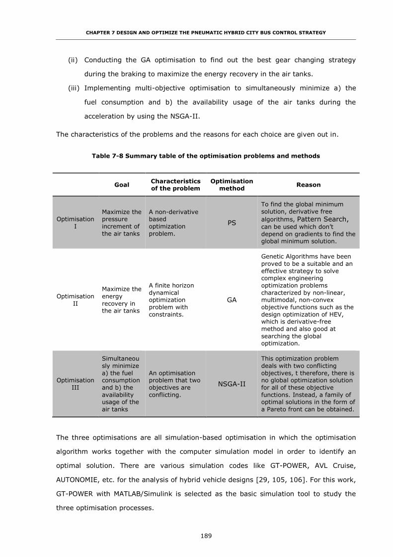
CHAPTER 7 DESIGN AND OPTIMIZE THE PNEUMATIC HYBRID CITY BUS CONTROL STRATEGY
189
(ii) Conducting the GA optimisation to find out the best gear changing strategy
during the braking to maximize the energy recovery in the air tanks.
(iii) Implementing multi-objective optimisation to simultaneously minimize a) the
fuel consumption and b) the availability usage of the air tanks during the
acceleration by using the NSGA-II.
The characteristics of the problems and the reasons for each choice are given out in.
Table 7-8 Summary table of the optimisation problems and methods
Goal Characteristics of the problem
Optimisation method
Reason
Optimisation
I
Maximize the pressure
increment of
the air tanks
A non-derivative based
optimization
problem.
PS
To find the global minimum
solution, derivative free
algorithms, Pattern Search, can be used which don’t
depend on gradients to find the global minimum solution.
Optimisation
II
Maximize the
energy
recovery in the air tanks
A finite horizon
dynamical optimization
problem with
constraints.
GA
Genetic Algorithms have been
proved to be a suitable and an
effective strategy to solve complex engineering
optimization problems
characterized by non-linear, multimodal, non-convex
objective functions such as the
design optimization of HEV, which is derivative-free
method and also good at
searching the global optimization.
Optimisation
III
Simultaneou
sly minimize
a) the fuel consumption
and b) the
availability usage of the
air tanks
An optimisation problem that two
objectives are
conflicting.
NSGA-II
This optimization problem
deals with two conflicting
objectives, t therefore, there is no global optimization solution
for all of these objective
functions. Instead, a family of optimal solutions in the form of
a Pareto front can be obtained.
The three optimisations are all simulation-based optimisation in which the optimisation
algorithm works together with the computer simulation model in order to identify an
optimal solution. There are various simulation codes like GT-POWER, AVL Cruise,
AUTONOMIE, etc. for the analysis of hybrid vehicle designs [29, 105, 106]. For this work,
GT-POWER with MATLAB/Simulink is selected as the basic simulation tool to study the
three optimisation processes.

CHAPTER 7 DESIGN AND OPTIMIZE THE PNEUMATIC HYBRID CITY BUS CONTROL STRATEGY
190
Another important question about the simulation, that of time duration needs to be
explained here. When conducting the GT-POWER and MATLAB/Simulink co-simulation, 1
s simulation time takes 1 min real time on a current technology desktop PC because the
detailed engine model is particularly onerous. For the selected driving cycle,
Braunschweig-H, running one single simulation takes almost 50 min real time. As a result,
the high number of simulations per generation that are required to be calculated, may
require a long elapsed time. Distributed computing is one way to solve this problem but
cannot be realized because GT-POWER cannot partition this type of simulation into
multiple nodes. Therefore, for all three types of optimisation, the optimisation has been
configured with particular care so as to limit the total simulation time while allowing the
optimisation target to be reached.
7.4.1 Optimize the Initial Air Tank Pressure for Every Stop-Start Event by
Using the Pattern Search Optimisation Method
Because the initial air tank pressure for every stop-start event strongly influences the
amount of energy recovery during the stop-start event, parameters in the control
strategy of the pneumatic hybrid city bus form a clear target for optimisation. The PS
algorithm is chosen here to identify optimal initial air tank pressure for every stop-start
event in order to maximize the pressure increment of the air tanks.
7.4.1.1 Pattern Search
For the optimisation problems for which the objective function is not differentiable or is
not even continuous, the direct search may be used [83]. Direct search can solve the
optimisation problems without any information about the gradient of the objective
function. Unlike more traditional optimisation methods that use information about the
gradient or higher derivatives to search for an optimal point, a direct search algorithm
searches a set of points around the current point, looking for one where the value of the
objective function is lower [83].
The direct search algorithm chosen here is called the Generalized Pattern Search
algorithm. The GPS algorithm computes a sequence of points to approach an optimal
point. At each step, the algorithm searches a set of points, called a mesh, around the
current point which is computed in the previous step of the algorithm. The mesh is

CHAPTER 7 DESIGN AND OPTIMIZE THE PNEUMATIC HYBRID CITY BUS CONTROL STRATEGY
191
formed by adding the current point to a scalar multiple of a set of vectors referred to as a
pattern. If the pattern search algorithm finds a point in the mesh that improves the
objective function at the current point, the new point becomes the current point at the
next step of the algorithm [83]. The algorithm will stop when the stopping criteria are
met. The definition of PS steps such as polling, expanding and contracting and the
particular method used to implement the PS optimisation are introduced in Appendix-V.
7.4.1.2 Problem Statement
The objective of this optimisation is to identify the initial air tanks pressure to increase
the total air tank pressure increment for a single start-stop manoeuvre, Braunschweig-H.
The cost function is defined as Equation (7-19):
𝐽 = 𝑚𝑎𝑥𝑓(𝑋) = 𝑚𝑖𝑛 [− (𝐽𝑝𝑟𝑒𝑠𝑠𝑢𝑟𝑒(𝑋))] = 𝑚𝑖𝑛[−(∫ �̇�𝑝𝑑𝑡)] (7-19)
where, Jpressure is the instantaneous pressure increment of two air tanks per unit time,
X is the variable vector which includes the parameters of the control strategy and is
shown in Table 7-9.
Table 7-9 Design variables for PS optimisation
Design
variable Description
Lower bound
(bar)
Upper bound
(bar)
p1 The initial pressure of air
tank 1 5.2 10
p2 The initial pressure of air
tank 2 2.5 10
In MATLAB, the Global Optimisation Toolbox optimisation functions minimize the
objective or fitness function [83]. As the optimisation is to find out the maximum air tank
pressure increment, it means the optimisation should minimize –f(x) as shown in
Equation (7-19). This is because the point at which the minimum of –f(x) occurs is the
same as the point at which the maximum of f(x) occurs [83].
The bounds of the two variables need to be explained here. In order to drive the air
motor to crank the engine, the lowest air tank need to above 5.2 bar. As a result, one air

CHAPTER 7 DESIGN AND OPTIMIZE THE PNEUMATIC HYBRID CITY BUS CONTROL STRATEGY
192
tank’s lower bound set to be 5.2 bar. The air tank is designed to have a maximum
operation pressure of 10 bar, as a result, the maximum air tank pressure should not be
above 10 bar [35]. Therefore, the upper bound for both air tanks is 10 bar. As mentioned
in Chapter 6, the air tank pressure needs to be above 2.5 bar to retain sufficient air to
realize the Boost Function. So the lower bound on the pressure of the other air tank
pressure is 2.5 bar. Start point, the initial point at which the algorithm starts the
optimisation, is an important parameter for the optimisation. In Global Optimisation
Toolbox, most solvers require to provide a starting point for the optimisation is because
that they require a start point to obtain the dimension of the decision variables [83]. The
start point of this optimisation is 7.5 and 6 which are both the median of their interval.
This means the two air tank initial pressure are set at the 7.5 bar for air tank 1, and 6
bar for air tank 2.
The PS optimisation parameter and options are summarized in Table 7-10.
Table 7-10 Summary table for PS optimisation
Solver patternserach – Pattern Search
Start point [7.5 6]
Lower bound [5.2 2.5]
Upper bound [10 10]
Poll methods GPS Positive basis 2N
Complete poll off
Polling order Consecutive
Max iterations 30
Function tolerance 0.01
7.4.1.3 Pattern Search Optimisation Result
Table 7-11 shows the PS optimisation result. The total pressure increment of two air
tanks during the specific driving cycle, Braunschweig-H, increases from 0.97 bar to 1.42
bar which means the amount of energy recovery has been improved 31.7%. The
negative value of the fitness value is because MATLAB can only minimize the objective,
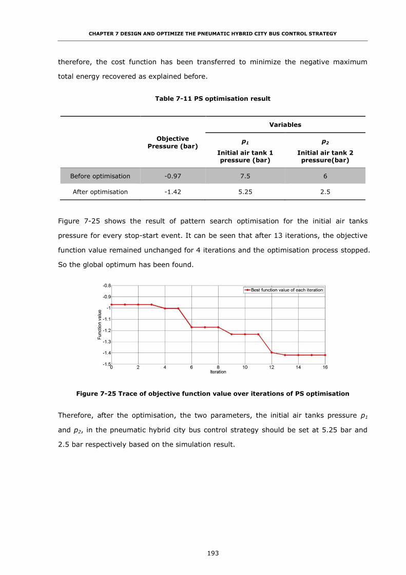
CHAPTER 7 DESIGN AND OPTIMIZE THE PNEUMATIC HYBRID CITY BUS CONTROL STRATEGY
193
therefore, the cost function has been transferred to minimize the negative maximum
total energy recovered as explained before.
Table 7-11 PS optimisation result
Objective
Pressure (bar)
Variables
p1
Initial air tank 1 pressure (bar)
p2
Initial air tank 2 pressure(bar)
Before optimisation -0.97 7.5 6
After optimisation -1.42 5.25 2.5
Figure 7-25 shows the result of pattern search optimisation for the initial air tanks
pressure for every stop-start event. It can be seen that after 13 iterations, the objective
function value remained unchanged for 4 iterations and the optimisation process stopped.
So the global optimum has been found.
Figure 7-25 Trace of objective function value over iterations of PS optimisation
Therefore, after the optimisation, the two parameters, the initial air tanks pressure p1
and p2, in the pneumatic hybrid city bus control strategy should be set at 5.25 bar and
2.5 bar respectively based on the simulation result.

CHAPTER 7 DESIGN AND OPTIMIZE THE PNEUMATIC HYBRID CITY BUS CONTROL STRATEGY
194
7.4.2 Optimisation of the Gear Changing Strategy during the Braking for
Best Energy Recovery Efficiency by Conducting the Genetic Algorithm
Optimisation Method
During the braking period, the bus can work in a regenerative braking mode to convert
kinetic energy to pneumatic energy by compressing air into air tanks. As discussed in
Chapter 3, the engine speed has the relationship with the engine brake performance and
the amount of pneumatic energy recovered during braking. Therefore, choosing different
gears to obtain different engine speed during the braking can significantly affect the
energy recovery efficiency. As a result, the gear shift-down points during the braking are
the critical parameters in the control strategy of the pneumatic hybrid city bus and
should be optimized.
As mentioned before, the hybrid system control problem can be considered as a difficult
optimisation problem which includes the constraints and real-valued objective function,
and may have many local optimums which mean that the gradient-based optimisation
algorithm may not converge to a global solution [82, 107]. The GA can be applied to
solve a variety of optimisation problems that are not well suited for standard optimisation
algorithms, such as the problems in which the objective function is discontinuous, non-
differentiable, stochastic, or highly nonlinear, and has the advantages of robust character
and global character for the non-linear problem of component optimisation [83, 108].
So the Single Objective Genetic Algorithm (SOGA) is chosen here to optimize the gear
shift-down points during the braking to maximize the energy recovery of air tanks during
one specific driving cycle, Braunschweig-H.
7.4.2.1 Genetic Algorithm
The concept of the GA, was developed by Holland and his colleagues in the 1960s and
1970s [109], is a kind of heuristic searching algorithm based on mechanics of natural
selection and natural genetics. GA is inspired by the evolutionist theory explaining the
origin of species [110]. In nature, the strong species have a greater opportunity to
deliver their genes to future generations via reproduction than the weak and unfit species.
After generation by generation, the species which carry the correct combination in their
genes become dominant in their population. But, genes may randomly change. If the

CHAPTER 7 DESIGN AND OPTIMIZE THE PNEUMATIC HYBRID CITY BUS CONTROL STRATEGY
195
changes provide additional advantages in the challenge for survival, new species evolve
from the old ones. Unfit species become extinct by natural selection. The terminology of
GA is shown in the Table 7-12.
Crossover and mutation are the two most important operators of GA. By iteratively
applying the crossover operator, genes of good chromosome are expected to appear
more frequently in the population, eventually leading to convergence to an overall good
solution [110]. Mutation plays a critical role in GA which reintroduces genetic diversity
back into the population and assists the search escape from the local optima. The
procedure of a generic GA is given as follow [111]:
Step 1: Set t = 1. Randomly generate N solutions to form the first population, P1.
Evaluate the fitness of solutions in P1.
Step 2: Crossover: Generate an offspring population Qt as follows:
2.1. Choose two solutions x and y from Pt based on the fitness values.
2.2. Using a crossover operator, generate offspring and add them to Qt.
Step 3: Mutation: Mutate each solution x ∈ Qt with a predefined mutation rate.
Step 4: Fitness assignment: Evaluate and assign a fitness value to each solution
x ∈ Qt based on its objective function value and infeasibility.
Step 5: Selection: Select N solutions from Qt based on their fitness and copy
them to Pt+1.
Step 6: If the stopping criterion is satisfied, terminate the search and return to
the current population, else, set t = t + 1 go to Step 2.

CHAPTER 7 DESIGN AND OPTIMIZE THE PNEUMATIC HYBRID CITY BUS CONTROL STRATEGY
196
Table 7-12 The terminology of GA
Name Definition
Fitness Functions The fitness function is the function need to be optimized.
Individuals or
chromosome A solution vector which can apply the fitness function.
Populations A collection of individuals.
Generations
At each iteration, the genetic algorithm performs a series of computations
on the current population to produce a new population. Each successive
population is called a new generation.
Diversity Diversity refers to the average distance between individuals in a
population.
Parents and
Children
To create the next generation, the genetic algorithm selects certain
individuals in the current population, called parents, and uses them to create individuals in the next generation, called children.
Genes The discrete units which constitute chromosome.
Crossover Two chromosomes are combined together to form new chromosomes.
Mutation Random changes into characteristics of chromosomes.
In the GA optimisation process implemented here, the fitness function and options of GA
is first input by using the Global Optimisation Toolbox in MATLAB and then the Global
Optimisation Toolbox completes the genetic steps such as generating the initial
population, selection, crossover and mutation to implement the optimisation. The
objective function and constraints are calculated using the GT-POWER and
MATLAB/Simulink co-simulation model. The flow chart of optimisation simulation is
shown in Figure 7-26. The simulation model is embedded into the optimisation procedure.
Each set of control parameters is created by the GA and supplied to the simulation. The
fitness function value is obtained from running the simulation model with the specific
driving cycle, Braunschweig-H.

CHAPTER 7 DESIGN AND OPTIMIZE THE PNEUMATIC HYBRID CITY BUS CONTROL STRATEGY
197
Figure 7-26 Flow chart of optimisation simulation model based on GA
7.4.2.2 Problem Statement
The objective of this optimisation is to select an optimal gear change strategy during the
deceleration process in order to increase the total energy recovered over a specific
driving cycle. The fitness function of the genetic algorithm for the pneumatic hybrid city
bus control strategy optimisation is defined as Equation (7-20):
𝐽 = 𝑚𝑎𝑥𝑓(𝑋) = 𝑚𝑖𝑛 [− (𝐽𝑒𝑛𝑒𝑟𝑔𝑦(𝑋))] = 𝑚𝑖𝑛[−(∫ 𝑚𝑎𝑖𝑟̇ 𝑑𝑡)] (7-20)
where, Jenergy is the instantaneous the amount of energy recovery of two air tanks per
unit time,
X is the variable vector which includes the parameters of the control strategy of
pneumatic hybrid city bus shown in Table 7-13.
Similar with the previous optimisation, the cost function has been transferred to minimize
–f(x) as shown in Equation (7-20).

CHAPTER 7 DESIGN AND OPTIMIZE THE PNEUMATIC HYBRID CITY BUS CONTROL STRATEGY
198
Table 7-13 Design variables for genetic algorithm optimisation
Design variable
Description Lower bound
(km/h) Upper bound
(km/h)
gear21 The gear shift-down point from
second to first gear 5 15
gear32 The gear shift-down point from
third to second gear 15 21
gear43 The gear shift-down point from
fourth to third gear 21 36
gear54 The gear shift-down point from
fifth to fourth gear 36 58
The start point of this optimisation is 10, 15, 30 and 45 which are the speed (km/h) that
gear shift-down points during the deceleration process. This gear change strategy during
the braking comes from previous research in Chapter 4 and calculated from the gear
ratios to fit the gear change requirement of the Braunschweig driving cycle.
The GA optimisation parameter and options are summarized in Table 7-14.
Table 7-14 Summary table for GA optimisation
Solver ga – Genetic Algorithm
Number of variable 4
Lower bound [5 15 21 36]
Upper bound [15 21 36 58]
Population size 20
Stall generations 15
7.4.2.3 Genetic Algorithm Optimisation Result
Table 7-15 shows the GA optimisation result. Figure 7-27 shows the GA optimisation
result after 26 generations with 20 individuals in each generation. The entire optimisation
process of the GA algorithm took approximately 520 hours (22 days) to complete. This
huge process time is not due to the GA but because of the large time GT-POWER takes to
emulate each design point.
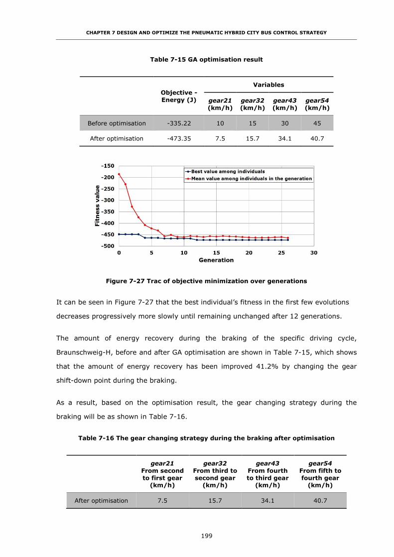
CHAPTER 7 DESIGN AND OPTIMIZE THE PNEUMATIC HYBRID CITY BUS CONTROL STRATEGY
199
Table 7-15 GA optimisation result
Objective -
Energy (J)
Variables
gear21
(km/h)
gear32
(km/h)
gear43
(km/h)
gear54
(km/h)
Before optimisation -335.22 10 15 30 45
After optimisation -473.35 7.5 15.7 34.1 40.7
Figure 7-27 Trac of objective minimization over generations
It can be seen in Figure 7-27 that the best individual’s fitness in the first few evolutions
decreases progressively more slowly until remaining unchanged after 12 generations.
The amount of energy recovery during the braking of the specific driving cycle,
Braunschweig-H, before and after GA optimisation are shown in Table 7-15, which shows
that the amount of energy recovery has been improved 41.2% by changing the gear
shift-down point during the braking.
As a result, based on the optimisation result, the gear changing strategy during the
braking will be as shown in Table 7-16.
Table 7-16 The gear changing strategy during the braking after optimisation
gear21
From second
to first gear (km/h)
gear32
From third to
second gear (km/h)
gear43
From fourth
to third gear (km/h)
gear54
From fifth to
fourth gear (km/h)
After optimisation 7.5 15.7 34.1 40.7

CHAPTER 7 DESIGN AND OPTIMIZE THE PNEUMATIC HYBRID CITY BUS CONTROL STRATEGY
200
7.4.3 Optimisation of the Gear Changing Strategy during Vehicle
Acceleration
The condition for activating the Boost Function is when the vehicle is in the full
acceleration mode while the driver demands 100% accelerator pedal position signal.
Normally, this happens after every gear change. Because of the Boost Function’s
capability to improve the engine transient response and reduce the fuel consumption, the
gear up-shift point can be changed. But with more Boost Function operations, there is a
greater loss of available energy from the air tanks. As a result, the gear change strategy
during acceleration will affect the fuel consumption and availability in the air tanks
simultaneously.
The question as how to balance the two conflicting objectives, the fuel consumption and
the available energy in the air tanks, by optimizing the gear changing strategy during the
acceleration forms the research topic. The Non-dominated Sorting Genetic Algorithm II
developed by Deb et al. is used here [112]. As a result, a Pareto front for the gear
changing strategy during the acceleration is obtained. The relationship between fuel
consumption and the availability usage, the optimal Pareto points and the gear changing
strategy during the acceleration of the pneumatic hybrid city bus are analysed and
discussed in the following sections.
7.4.3.1 Multi-objective Genetic Algorithm Optimisation
The aim of multi-objective optimisation problems is to find the best candidate solutions
among multiple objective functions that are usually conflicting [19]. Multi-objective
formulations are realistic models for many complex engineering optimisation problems
[110]. In many engineering problems, the objectives, such as minimising cost,
maximising performance and reliability, tend to conflict with each other. Meeting a single
objective can lead to unacceptable results with respect to the other objectives. To
prevent this, the objectives should be simultaneous optimized. A reasonable approach to
a multi-objective requirement is to investigate a set of solutions, each of which satisfies
the objectives at an acceptable level without being dominated by any other solution
[110].

CHAPTER 7 DESIGN AND OPTIMIZE THE PNEUMATIC HYBRID CITY BUS CONTROL STRATEGY
201
There are two general approaches to multi-objective optimisation. The first is to combine
the individual objective functions into a single composite function or move all but one
objective to the constraint set [110]. In both cases of the first approach, an optimisation
method cannot return a set of solutions which can be examined for trade-offs, which only
can return a single solution. The second one is to determine an entire Pareto optimal
solution set or a representative subset [110]. A Pareto optimal set is a set of solutions
that are non-dominated with respect to each other. When moving from one Pareto
solution to another, there is always a certain amount of sacrifice in one objective(s) to
achieve a certain amount of gain in the other(s) [110]. The Pareto optimal solution set
are often preferred to single solutions because they can be practical when considering
real-life problems since the final solution of decision-maker is always a trade-off [110].
Evolutionary algorithms are the good candidate for multi-objective optimisation problems
due to their abilities, to search simultaneously for multiple Pareto optimal solutions and
perform the better global search of the search space [29]. GA, as the best-known branch
among existing evolutionary algorithms, is easy to use and implement because it uses
only a simple scalar performance measure that does not require or use derivate
information [30]. GA is well fitted for the requirements to solve a multi-objective
optimisation problem because it is a population-based approach. Due to evolutionary
algorithms’ inherent parallelism, they are able to capture a number of solutions
concurrently in a single run [113]. These mean a) if problem has single optimum,
population members can be expected to converge to optimum, and b) if it has multiple
optimal solutions, capture multiple optimal solutions in its final population [114]. There
are several advantages for GA to solve the multi-objective problems.
(i) The ability of GA to simultaneously search different regions of a solution space
makes it possible to find a diverse set of solutions for different problems with
non-convex, discontinuous, and multi-modal solutions spaces [110].
(ii) The crossover operator of GA may exploit structures of good solutions with
respect to different objectives to create new non-dominated solutions in
unexplored parts of the Pareto front [110].
(iii) Most multi-objective GA do not require the user to prioritize, scale, or weigh
objectives [110].

CHAPTER 7 DESIGN AND OPTIMIZE THE PNEUMATIC HYBRID CITY BUS CONTROL STRATEGY
202
As a result, GA has been the most popular heuristic approach to multi-objective design
and optimisation problems [110]. Since the first multi-objective GA, called vector
evaluated GA, was proposed by Schaffer [115], several multi-objective evolutionary
algorithms have been developed such as Multi-objective Genetic Algorithm (MOGA),
Nondominated Sorting Genetic Algorithm (NSGA), Strength Pareto Evolutionary
Algorithm (SPEA), and Fast NSGA-II [116-119]. A comprehensive experimental
methodology to quantitatively compare multi-objective optimizers has been presented by
Zitzler [120]. The widespread opinions that a) multi-objective evolutionary algorithms
can have clear advantages over traditional multi-criteria optimisation methods, and ii)
NSGA-II and SPEA clearly outperformed other MOEA implementations on the test
problems, had been substantiated experimentally [120]. The NSGA-II is chosen for this
multi-objective optimisation problem because the NSGA-II, in most problems, is able to
find a much better spread of solutions and better convergence near the true Pareto-
optimal front compared to other multi-objective evolutionary algorithms [119]. The use
of NGSA-II makes it possible to obtain the entire Pareto front of optimal the gear
changing strategy during the acceleration in a single optimisation run [121]. This is
beneficial not only from the computational standpoint, but also from the perspective of
picturing and understanding the trade-offs between the two objectives [121].
Similar to the implementation of the SOGA optimisation in the last section, the Global
Optimisation Toolbox in MATLAB is used for multi-objective optimisation in this research.
The fitness functions and options of the optimisation problem are notified to the Global
Optimisation Toolbox. Then the Global Optimisation functions complete the genetic steps:
generating the initial population, selection, crossover and mutation to implement the
optimisation. The objective functions and constraints are calculated based on the GT-
POWER and MATLAB/Simulink model. The simulation model as a module is embedded
into the entire optimisation procedure for implementation, and it is completed in the time
domain. For each individual in each generation, the control parameters input to the
simulation model is created by NSGA-II, and the fitness functions value are obtained by
running the simulation model with the specific driving cycle, Braunschweig-H.

CHAPTER 7 DESIGN AND OPTIMIZE THE PNEUMATIC HYBRID CITY BUS CONTROL STRATEGY
203
7.4.3.2 Problem Statement
The mathematics description of multi-objective optimisation problem can be defined as
follows:
{min𝑋∈Ω 𝐹(𝑋) = [𝑓1(𝑋), 𝑓2(𝑋2), … , 𝑓𝑚(𝑋)]
𝑠. 𝑡. 𝑔𝑗(𝑋) ≥ 0 𝑗 = 1,2, … , 𝑛 (7-21) [122]
where, X=(x1, x2,…,xN) – a variable vector in a real and N-dimensional space,
Ω – feasible solution space,
fm(X) – objective functions for optimisation,
gj(X) – constraint functions which have already been defined in the GT-POWER
simulation model.
In this section, two bus operation optimisation objectives are considered over a driving
cycle:
(i) Fuel consumption,
(ii) Loss of available energy in the air tanks.
As a result, the fitness function of the multi-objective genetic algorithm for the
pneumatic hybrid city bus control strategy optimisation is defined as Equation (7-22):
𝐽 = 𝑚𝑖𝑛𝑑𝑟𝑖𝑣𝑖𝑛𝑔 𝑐𝑦𝑐𝑙𝑒 ∑ ∫ (�̇� + 𝜆�̇�𝑓)𝑇𝑁
0𝑁 (7-22)
The design variables for multi-objective optimisation are shown in Table 7-17.
Table 7-17 Design variables for multi-objective optimisation
Design
variable Description
Lower bound
(km/h)
Upper bound
(km/h)
gear12 The gear shift-up point from first to
second gear at vehicle speed 7.54 15
gear23 The gear shift-up point from second to
third gear at vehicle speed 15.7 21
gear34 The gear shift-up point from third to
fourth gear at vehicle speed 34.1 36
gear45 The gear shift-up point from fourth to
fifth gear at vehicle speed 40.7 58

CHAPTER 7 DESIGN AND OPTIMIZE THE PNEUMATIC HYBRID CITY BUS CONTROL STRATEGY
204
This optimisation approach deals with two conflicting objectives; while minimizing the
total fuel consumption requires more boost operations to increase the internal
combustion engine efficiency, the more boost operations tend to decrease the available
energy in the air tanks. Therefore, a single optimal point does not exist; instead, a family
of optimal solutions in the form of a Pareto front can be obtained, as presented next.
The GA does not require a start point for the optimisation and it will create one using the
Creation function [83]. As a result, in this optimisation, the start point is not specified.
The GA optimisation parameter and options are summarized in Table 7-18.
Table 7-18 Summary table for NSGA-II optimisation
Solver gamultiobj – Multiobjective optimization using
Genetic Algorithm
Number of variable 4
Lower bound [7.54 15.7 34.1 40.7]
Upper bound [15 21 36 58]
Population size 12 or 50
Pareto front population fraction 0.5
Generation 20 or 5
7.4.3.3 Multi-objective Optimisation Result
Two different options multi-objective optimisations has been carried out to represent how
the options will affect the optimisation result. These two optimisations both use the
NSGA-II and their differences of options are shown in Table 7-19. Generations specify
the maximum number of iterations the GA performs. Population size specifies how many
individuals are in each generation. From Table 7-19, it can be seen that the total
calculation times of two optimisations are almost same which are 240 and 250 iterative
respectively. The reason for choosing these two options is because of the duration of the
simulation time. The entire optimisation process for the NSGA-II algorithm to calculate
250 times took approximately 120 hours (5 days) to complete. This huge process time is
not due to the algorithm itself but because of the large time GT-POWER takes to emulate
each design point which has been already explained before. As a result, increasing the
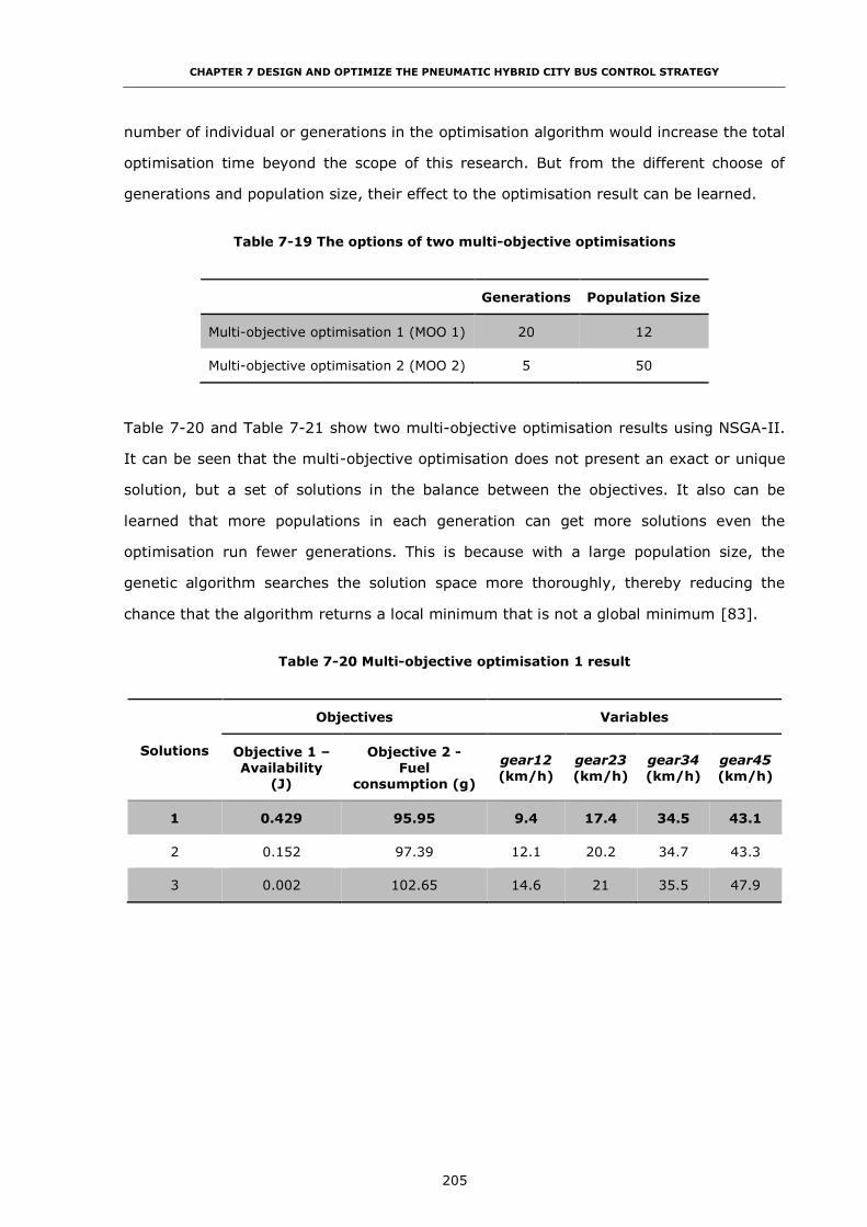
CHAPTER 7 DESIGN AND OPTIMIZE THE PNEUMATIC HYBRID CITY BUS CONTROL STRATEGY
205
number of individual or generations in the optimisation algorithm would increase the total
optimisation time beyond the scope of this research. But from the different choose of
generations and population size, their effect to the optimisation result can be learned.
Table 7-19 The options of two multi-objective optimisations
Generations Population Size
Multi-objective optimisation 1 (MOO 1) 20 12
Multi-objective optimisation 2 (MOO 2) 5 50
Table 7-20 and Table 7-21 show two multi-objective optimisation results using NSGA-II.
It can be seen that the multi-objective optimisation does not present an exact or unique
solution, but a set of solutions in the balance between the objectives. It also can be
learned that more populations in each generation can get more solutions even the
optimisation run fewer generations. This is because with a large population size, the
genetic algorithm searches the solution space more thoroughly, thereby reducing the
chance that the algorithm returns a local minimum that is not a global minimum [83].
Table 7-20 Multi-objective optimisation 1 result
Solutions
Objectives Variables
Objective 1 –
Availability
(J)
Objective 2 -
Fuel
consumption (g)
gear12
(km/h)
gear23
(km/h)
gear34
(km/h)
gear45
(km/h)
1 0.429 95.95 9.4 17.4 34.5 43.1
2 0.152 97.39 12.1 20.2 34.7 43.3
3 0.002 102.65 14.6 21 35.5 47.9

CHAPTER 7 DESIGN AND OPTIMIZE THE PNEUMATIC HYBRID CITY BUS CONTROL STRATEGY
206
Table 7-21 Multi-objective optimisation 2 result
Solutions
Objectives Variables
Objective 1 - Availability
(J)
Objective 2 - Fuel
consumption (g)
gear12
(km/h)
gear23
(km/h)
gear34
(km/h)
gear45
(km/h)
1 0.002 102.65 14.6 21.0 35.5 47.9
2 0.066 98.46 11.0 18.4 34.6 45.8
3 0.248 96.45 8.4 17.4 34.5 43.1
4 0.126 97.15 12.6 20.3 34.5 43.3
5 0.281 96.44 9.6 17.4 34.6 43.5
6 0.048 98.65 13.3 18.6 34.8 45.0
7 0.090 97.52 13.0 19.3 34.7 43.4
8 0.008 100.91 14.6 18.7 35.0 46.6
9 0.304 96.25 9.5 19.3 34.5 43.1
10 0.210 96.77 9.2 17.9 34.6 43.4
11 0.154 97.00 11.9 19.2 34.5 43.3
12 0.234 96.66 9.3 18.3 34.5 43.2
13 0.012 99.19 13.9 20.0 34.9 45.6
14 0.002 102.65 14.6 21.0 35.5 47.4
15 0.229 96.69 11.1 18.3 34.5 43.1
16 0.038 98.95 14.0 19.7 35.2 44.4
17 0.089 97.53 13.3 19.3 34.7 43.4
18 0.355 95.84 8.7 17.6 34.5 43.1
Figure 7-28 shows two Pareto front after optimisation. The MOO 1 result is marked with
the red square, and the red dash line shows an estimated Pareto front if both numbers of
individuals and generations are increased. The MOO 2 result is marked with the blue
triangle, and the blue dash line shows also an estimated Pareto front if both numbers of
individuals and generations are increased.

CHAPTER 7 DESIGN AND OPTIMIZE THE PNEUMATIC HYBRID CITY BUS CONTROL STRATEGY
207
Figure 7-28 Optimal Pareto front for the multi-objective optimisation using NSGA-II
From Figure 7-28, it can be seen that both in two Pareto fronts, a better fuel
consumption can be achieved with a high availability usage in the air tanks. For example,
for the multi-objective optimisation 1 result, the fuel consumption in the Pareto front
ranges between 95.95 to 102.65 g for a specific driving cycle, Braunschweig-H, while the
availability usage in the two air tanks varies from 0.02 to 0.429 J. The solution 2 which is
point 2 in Figure 7-28 represents a good compromise of fuel consumption and availability
usage in the air tanks. Lower fuel consumption would have to be paid for with a relative
bigger increase of availability usage in the air tanks supporting boost function operations.
One example is Solution 1 which is point 1 in Figure 7-28. It has the lowest fuel
consumption 95.95 g but the highest availability loss in the two air tanks which is 0.429 J
during one acceleration event. Compared with solution 1 and solution 3, it can be learned
that the fuel consumption can be improved 6.5%.
But from Figure 7-28, it also can be seen that the multi-objective optimisation 2 can get
a better solution which is Solution 18 in Table 7-21 and point 4 in Figure 7-28. This
solution has lower fuel consumption than solution 1 which is 95.84 g, and also has lower
availability loss than solution 1 in the two air tanks which is 0.355 J during one
acceleration event. This means compared with multi-objective optimisation 1, multi-
objective optimisation 2 can supply a better solution which uses less air in two tanks but
also has lower fuel consumption.
The result proves:
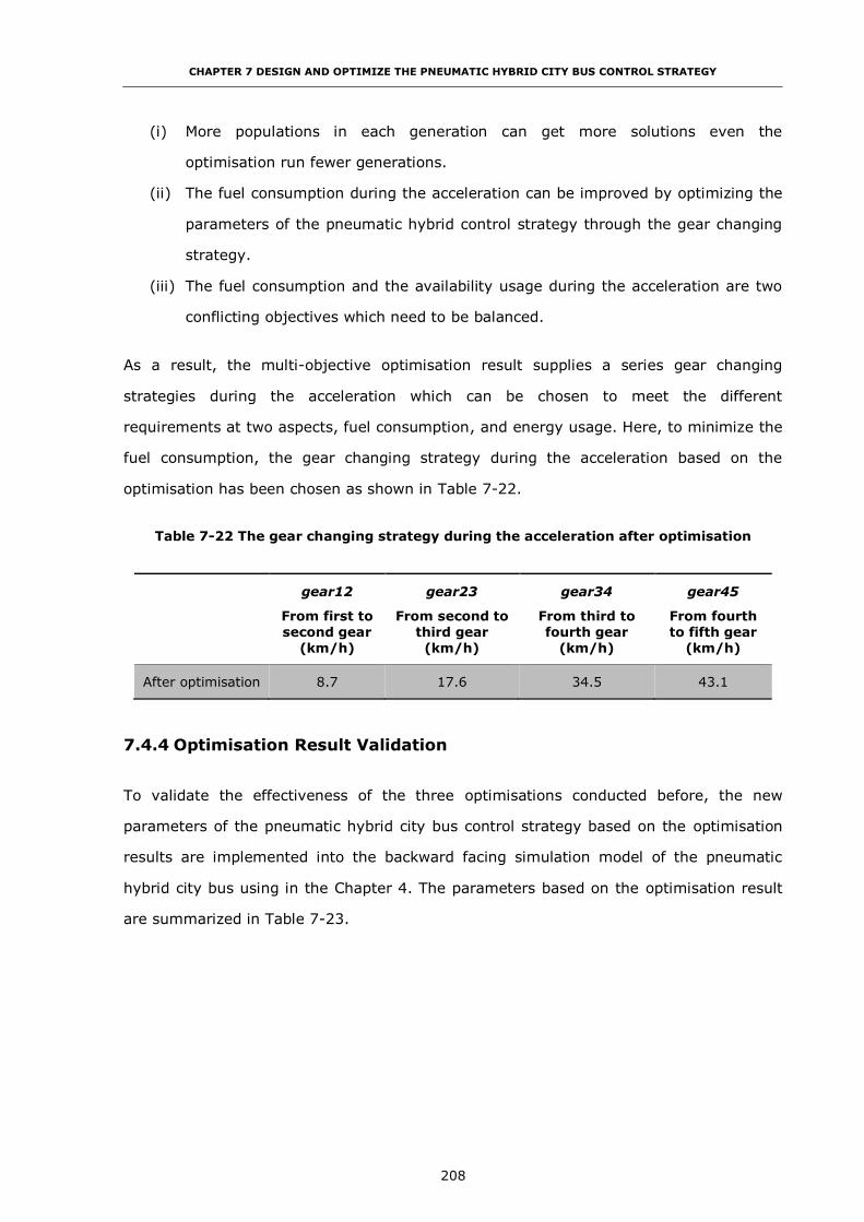
CHAPTER 7 DESIGN AND OPTIMIZE THE PNEUMATIC HYBRID CITY BUS CONTROL STRATEGY
208
(i) More populations in each generation can get more solutions even the
optimisation run fewer generations.
(ii) The fuel consumption during the acceleration can be improved by optimizing the
parameters of the pneumatic hybrid control strategy through the gear changing
strategy.
(iii) The fuel consumption and the availability usage during the acceleration are two
conflicting objectives which need to be balanced.
As a result, the multi-objective optimisation result supplies a series gear changing
strategies during the acceleration which can be chosen to meet the different
requirements at two aspects, fuel consumption, and energy usage. Here, to minimize the
fuel consumption, the gear changing strategy during the acceleration based on the
optimisation has been chosen as shown in Table 7-22.
Table 7-22 The gear changing strategy during the acceleration after optimisation
gear12
From first to
second gear
(km/h)
gear23
From second to
third gear
(km/h)
gear34
From third to
fourth gear
(km/h)
gear45
From fourth
to fifth gear
(km/h)
After optimisation 8.7 17.6 34.5 43.1
7.4.4 Optimisation Result Validation
To validate the effectiveness of the three optimisations conducted before, the new
parameters of the pneumatic hybrid city bus control strategy based on the optimisation
results are implemented into the backward facing simulation model of the pneumatic
hybrid city bus using in the Chapter 4. The parameters based on the optimisation result
are summarized in Table 7-23.

CHAPTER 7 DESIGN AND OPTIMIZE THE PNEUMATIC HYBRID CITY BUS CONTROL STRATEGY
209
Table 7-23 Parameters in the pneumatic hybrid city bus control strategy after
optimisation
Initial air tanks pressure
Air tank 1 (bar) Air tank 2 (bar)
5.25 2.5
Gear change
strategy
Speed range (km/h)
During the acceleration During the braking
First gear 0 - 8.7 0 - 7.5
Second gear 8.7 - 17.6 7.5 - 15.7
Third gear 17.6 - 34.5 15.7 - 34.1
Fourth gear 34.5 - 43.1 34.1 - 40.7
Fifth gear >43.1 >40.7
The fuel consumption of the model running the whole Braunschweig driving cycle with
the control parameters before and after optimisations is shown in Table 7-24, which
shows that the fuel economy had been further improved 6.03%.
Table 7-24 Fuel consumption before and after optimisations
Driving cycle Fuel consumption
before
optimisations
Fuel consumption after
optimisations
Improvement
Braunschweig
driving cycle
39.93 l/100km 37.52 l/100km
6.03%
3171.8 g 2980.5 g
The improvement of fuel economy indicated that the optimisations implemented before
can be used to identify the best control parameters for the pneumatic hybrid city bus
control strategy to improve energy efficiency.
7.5 Conclusion
An energy control strategy based on the “logic threshold” methodology for the pneumatic
hybrid city bus has been designed. The control strategy can manage the pneumatic

CHAPTER 7 DESIGN AND OPTIMIZE THE PNEUMATIC HYBRID CITY BUS CONTROL STRATEGY
210
hybrid city bus to realize three special functions: Stop-Start, Boost, and Regenerative
Braking as well as the normal operations.
To analyse the pneumatic hybrid city bus dynamic performance, engine transient
response, fuel economy and energy usage, a forward facing pneumatic hybrid city bus
simulation model which includes the detailed engine model has been developed in GT-
POWER and MATLAB/Simulink co-simulation.
Three global optimisation algorithms, PS, GA and Multi-objective NSGA-II, are compared
and employed for the different optimisation processes required for the vehicle control
strategy. Optimisation criteria were selected from fuel consumption, air mass recovered
and the deployment of available energy during regeneration. As a result of identifying
optimal conditions – when compared with the original nominal design:
(i) The total pressure increment of two air tanks during the specific driving cycle,
Braunschweig-H, has been increased from 0.97 bar to 1.42 bar which means the
amount of energy recovery has been improved 31.7% by implementing the
pattern search optimisation to optimize the initial air tanks pressure for every
stop-start event.
(ii) The amount of energy recovery during the braking in Braunschweig-H, has been
improved 41.2% by modifying the gear shift-down point.
(iii) The fuel consumption and the availability usage in the air tanks during the
acceleration are two conflicting objectives which need to be balanced: the fuel
consumption can improve 6.5% by choosing the best result.
To verify the effectiveness of the optimisation result, an example simulation is carried out
by implementing the optimisation in a backward facing vehicle model. The simulation
result demonstrated that the fuel economy can be further improved by 6%. This result
shows that
(i) Compared with the fuel economy improvement 6.5% in the forward facing model,
the backward facing model confirms that 6% fuel consumption can be reduced.
The difference is because that in forward facing model, the fuel consumption is
calculated by the Braunschweig-H rather than the whole Braunschweig driving
cycle.

CHAPTER 7 DESIGN AND OPTIMIZE THE PNEUMATIC HYBRID CITY BUS CONTROL STRATEGY
211
(ii) The method that choosing one typical stop-start event, Braunschweig-H, to
represent the whole Braunschweig driving cycle as the test cycle for the
optimisation has been proved feasible. Although the improvements in fuel
consumption between the Braunschweig-H and Braunschweig driving cycle are
respectively 6.5% and 6% which means 8.3% difference, it still demonstrates
that the supposition that using the Braunschweig-H as an alternative to
Braunschweig driving cycle.
CHAPTER 8 CONCLUSION AND FUTURE PROSPECTS
212
CHAPTER 8
CONCLUSION AND FUTURE PROSPECTS
To respond to the fact that there is as yet no in-depth study on how to implement the
pneumatic hybrid technology on the city bus, the aim of the reported research has been
to develop an understanding of the pneumatic hybrid powertrain system and its control
strategy. One important aspect is the demonstration of the ability of such systems to
improve upon the conventional Powertrain technology. Section 8.1 summarizes the
notable conclusions of the study, while Section 8.2 includes an introduction and
discussion concerning the improvements, suggestions and recommendations for future
work on the pneumatic hybrid technology.
8.1 Conclusion
The works that have been done and the results achieved are listed with the
corresponding research aims and objectives listed in Chapter 1.
(i) To fully understand the principle of the operation of the pneumatic hybrid engine
and the quantification of the sensitivity of the work done to design parameters
during the Compressor Mode.
This objective has been achieved in Chapter 3. The principle of operation has
been presented. The potential of the pneumatic hybrid system both to generate
a supply of compressed air and to manage the contribution of the engine to
vehicle braking had been confirmed. The pneumatic hybrid engine CM is
considered from a theoretical perspective based on an air cycle analysis and
validated. An understanding of the sensitivity of work done (braking torque
created during the CM) to design parameters is given. The results demonstrate
a) The lower air tank pressure can create more brake torque at the same engine
speed,
CHAPTER 8 CONCLUSION AND FUTURE PROSPECTS
213
b) The longer CREB intake valve second opening duration decreases the brake
torque performance,
c) It always has the maximum engine brake torque output when the CREB intake
valve second closing time is right at TDC which means IVSC is 0°CA.
(ii) To evaluate the fuel economy improvement ability of pneumatic hybrid
technology for the city bus through different bus driving cycles.
This objective has been fulfilled in Chapter 4. An evaluation of the fuel economy
improvement ability of pneumatic hybrid technology for the city bus application
by realizing the Stop-Start Function through different bus driving cycles has
been presented. Also, an investigation is made into how multiple air tanks give
an additional degree of freedom for management of recovered air. A backward-
facing simulation model of the city bus with the pneumatic hybrid powertrain has
been applied to investigate the improvement of fuel economy by using one and
two air tanks in different driving cycles in Simulink with Stateflow. The analysis
shows
a) The pneumatic hybrid technology can reduce fuel consumption by at least 6%
through stop-start operation, and can eliminate 90% of the idling time,
b) In the case of the modelled bus cycles, significant fuel savings of 7.1% can be
achieved during MLTB driving cycles because of the large braking energy and
frequent stop–start operations required during the type of bus operation
exemplified by this cycle,
c) The two air tanks pneumatic hybrid system has the higher fuel saving
potential which is because it can offer the possibility of at least one air tank’s
pressure being higher than the lower limit and other lower pressure air tank
results in higher energy capture during the CM.
(iii) To analyse engine braking characteristics during the vehicle’s deceleration and
braking process during different bus driving cycles and hence identify
appropriate braking system structure and its control strategies for maximum
energy recovery.

CHAPTER 8 CONCLUSION AND FUTURE PROSPECTS
214
This objective has been achieved in Chapter 5. It firstly presents an analysis of
vehicle braking behaviour through different bus driving cycles and compares two
configurations of the hybrid braking system, the parallel hybrid brake system
and the fully controllable hybrid brake system. The comparison shows the fully
controllable hybrid braking system has a distinct advantage and is chosen to
realize the Regenerative Braking Function. A braking simulation model has been
built in to support an investigation of an optimum air tank pressure and
configuration for energy recovery. Based on the optimisation result, a new
control strategy is implemented along with a baseline simulation model to
explore the benefits of the new control strategy. The findings include
a) It indicates that in the urban area the bus’s braking power can reach to 80%
of the total traction power, and the braking of the city bus is very gentle with
most of the deceleration rate below 0.2 g, compared with the passenger car,
b) The fully controllable hybrid braking system is fit for the requirement of the
pneumatic hybrid regenerative system which can either work at high efficiency to
recover as much braking energy as possible and supply the corresponding
braking force,
c) The optimisation result shows that the 5.2 bar air tank pressure is the best
pressure for braking energy recovery,
d) The model with the newly optimized initial air tanks pressure can enhance 2.7%
the total air mass recovered during the braking compared with the previous
control strategy which means the air tanks pressure is the function of the energy
recovery rate.
(iv) To study the benefits of extra boost on reducing turbo-lag, improved engine
performance, and reduce fuel consumption.
This objective has been achieved in Chapter 6. An analysis of the reasons for
engine turbo-lag and the methods developed for reducing the turbo-lag and
improving transient response have been presented first. Then, a number of
architectures for managing a rapid energy transfer into the powertrain to assist

CHAPTER 8 CONCLUSION AND FUTURE PROSPECTS
215
acceleration of the turbocharger have been proposed and investigated from two
aspects, engine brake torque response and vehicle acceleration, by using the 1-
D engine simulation. The findings show
a) The System I, IP and E all improve torque response time (to maximum torque)
by 90.8%, 78.3% and 80.8% respectively, when the engine accelerates from no
load to full load at 1600 rpm, and both the Systems I and IP can be seen to
significantly reduce the vehicle acceleration time, from 0 to 48 km/h, 13% and
8.6% respectively through reduction of turbo-lag,
b) System I carries the highest risk of compressor surge. System IP carries a
lower risk of surge because it does not block the output of the compressor.
System E has no risk of surge because it does not need a valve in the intake
system,
c) System IP offers considerable advantages over System I at both less use of
air and less likely to cause the compressor surge.
(v) To formulate a pneumatic hybrid city bus control strategy and the vehicle driving
cycle simulation programme and identify the relationship between respectively
the operating parameters, fuel consumption and energy usage according to
optimisation criteria.
This objective has been achieved in Chapter 7. An energy control strategy based
on the use of thresholds in the degree of energy storage and regeneration (a
“logic threshold” methodology) for the pneumatic hybrid city bus has been
designed. A forward facing pneumatic hybrid city bus simulation model which
includes the detailed engine model has been developed in GT-POWER with
MATLAB/Simulink co-simulation. To obtain the maximum overall fuel economy,
the amount of air and energy recovered during the braking and minimum loss of
availability during acceleration, a number of variables in the control strategy
must be optimized. Three global optimisation algorithms, Pattern Search,
Genetic Algorithm and multi-objective Non-dominated Sorting Genetic Algorithm
II are compared and employed for the optimisation of the control strategy
considered at three levels respectively. The results show

CHAPTER 8 CONCLUSION AND FUTURE PROSPECTS
216
a) The proposed energy control strategy for the pneumatic hybrid city bus
enables the vehicle to realize the specific functions: Stop-Start, Boost and
Regenerative braking, as well as the normal operation of the vehicle,
b) The total pressure increment of two air tanks during the specific driving cycle,
Braunschweig-H, has been increased from 0.97 bar to 1.42 bar which means the
amount of energy recovery has been improved 31.7% by implementing the PS
optimisation to optimize the initial air tanks pressure for every stop-start event,
c) The amount of energy recovery during the braking in Braunschweig-H, has
been improved 41.2% by modifying the gear shift-down point,
d) The fuel consumption and the availability usage in the air tanks during the
acceleration are two conflicting objectives which need to be balanced: the fuel
consumption can improve 6.5% by choosing the best multi-objective
optimisation result,
e) By optimizing the variables in the control strategy, the fuel economy of a
pneumatic hybrid city bus can be further improved by 6%,
f) The method that choosing one typical stop-start event, Braunschweig-H, to
represent the whole Braunschweig driving cycle as the test cycle for the
optimisation has been proved feasible.
It can be concluded that the effectiveness of the pneumatic hybrid technology has been
successfully proved by this study. The pneumatic hybrid technology can improve the city
bus fuel economy by at least 6% for a typical bus driving cycle, reducing the engine
brake torque response time and improving acceleration. The pneumatic hybrid
technology offers an alternative to the electric hybrid. It offers significant advantages,
such as good fuel economy, and vehicle drivability improvement. Unlike the electric
hybrid, pneumatic hybrid technology can be implemented without adding a new
propulsion system to the vehicle, it has demonstrable advantages in manufacturing cost,
lower mass, and suitability for commercially viable large volume production.
CHAPTER 8 CONCLUSION AND FUTURE PROSPECTS
217
8.2 Recommendations for Future Works
Due to limited time and words, this PhD thesis can only discuss those explained above.
However around this technology, there have been still numbers of issues worthy to be
explored further, for instance:
(i) In order to validate the modelling work in Chapter 3 and Chapter 6, the engine
experimental tests should be carried out on a single cylinder engine to verify the
Chapter 3 model and results, and a six-cylinder engine to validate the Chapter 6
model and findings.
(ii) Further optimisation of operating parameters such as auxiliary chamber size, air
tank(s) volume and valve timing would be desirable by means of more extensive
systematic studies to fully evaluate the pneumatic hybrid system potential in fuel
savings and vehicle performance improvement.
(iii) The pneumatic hybrid city bus control strategy can be further developed by
importing the telemetry data, such as using an electronic horizon generated via
the GPS data. Then the route profiles and traffic conditions can be calculated,
thus allowing the control strategy to be optimized to enhance the energy
efficiency.
(iv) How to start the engine by injecting compressed air into the individual cylinders
to propel the pistons during the cranking to replace the air starter using in this
research to further reduce the cost of the pneumatic hybrid system.
(v) The compressed air used in combination with EGR technology in a diesel engine
to improve the dynamic trade-off between NOx and smoke emissions.
(vi) Investigations could also look at the possibility of implementing the pneumatic
hybrid system as an exhaust energy recovery device, thus further improving the
energy efficiency by recovering the useful energy in the exhaust gas.
(vii) Finally, for simulation purpose the valves are idealised in this research. Flow
losses and valve dynamics are neglected. However, a detailed investigation will
need to consider valve behaviour in order to evaluate the detailed effect on
systems response and the fuel economy gains. Also valve operating procedures
which change air flow in manifolds and the engine cylinders, changing the
patterns of losses requires further investigation in the future work.
REFERENCE
218
REFERENCE
[1] I. E. Agency, "CO2 Emissions from Fuel Combustion 2014 - Highlights," Retrieved
from
https://www.iea.org/publications/freepublications/publication/CO2EmissionsFromFuelCo
mbustionHighlights2014.pdf, Last accessed: March 24, 2015, 2014.
[2] U. Tietge and P. Mock, "CO2 emissions from new passenger cars in the EU: Car
manufacturers’ performance in 2013," Retrieved from
http://www.theicct.org/sites/default/files/publications/ICCTbriefing_EU-CO2_201406.pdf,
Last accessed: March 24, 2015, 2014.
[3] T. V. Johnson, "Vehicular Emissions in Review," SAE Int. J. Engines, vol. 5, pp.
216-234, 2012.
[4] C. Lee, "Computational and experimental study of air hybrid engine concepts,"
PhD Thesis, Brunel University London, 2011.
[5] E. D. Tate, M. O. Harpster, and P. J. Savagian, "The Electrification of the
Automobile: From Conventional Hybrid, to Plug-in Hybrids, to Extended-Range Electric
Vehicles," SAE Int. J. Passeng. Cars - Electron. Electr. Syst., vol. 1, pp. 156-166, 2008.
[6] M. Ehsani, Y. Gao, and A. Emadi, Modern Electric, Hybrid Electric, and Fuel Cell
Vehicles: Fundamentals, Theory, and Design, Second Edition. Boca Raton: CRC Press,
2009.
[7] T. Christen and M. W. Carlen, "Theory of Ragone plots," Journal of power sources,
vol. 91, pp. 210-216, 2000.
[8] S. Miller, "AQMD Hydraulic Hybrid Vehicle Forum and Technical Roundtable,"
International Truck and Engine, ovember, vol. 15, 2007.
[9] X. Zeng, "Improving the energy density of hydraulic hybridvehicle (HHVs) and
evaluating plug-in HHVs," 2009.
REFERENCE
219
[10] S. Ranganathan, "HYBRID BUSES COSTS AND BENEFITS," Retrieved from
http://www.eesi.org/files/eesi_hybrid_bus_032007.pdf, Last accessed: December 26,
2015.
[11] R. Bao and R. Stobart, "Using Pneumatic Hybrid Technology to Reduce Fuel
Consumption and Eliminate Turbo-Lag," SAE Technical Paper 2013-01-1452, 2013.
[12] T. Liu, J. Zheng, S. Wang, and F. Gu, "Logic Threshold Based Energy Control
Strategy for Parallel Hydraulic Hybrid Vehicles," Research Journal of Applied Sciences,
Engineering and Technology, vol. 6, pp. 2339-2344, 2013.
[13] R. Prohaska, A. Duran, A. Ragatz, and K. Kelly, "Statistical Characterization of
Medium-Duty Electric Vehicle Drive Cycles," 2015.
[14] P. Higelin, A. Charlet, and Y. Chamaillard, "Thermodynamic Simulation of a Hybrid
Pneumatic-Combustion Engine Concept," Int.J. Applied Thermodynamics, vol. 5, p. 11,
2002.
[15] M. M. Schechter, "New Cycles for Automobile Engines," SAE Techincal Paper
1999-01-0623, 1999.
[16] L. Guzzella and A. Sciarretta, Vehicle propulsion systems : introduction to
modeling and optimization. Berlin: Berlin : Springer, 2007.
[17] C. Tai, T. Tsao, M. B. Levin, G. Barta, and M. M. Schechter, "Using Camless
Valvetrain for Air Hybrid Optimization," SAE Techincal Paper 2003-01-0038, 2003.
[18] J. W. G. Turner, M. D. Bassett, R. J. Pearson, G. Pitcher, and K. J. Douglas, "New
Operating Strategies Afforded by Fully Variable Valve Trains," SAE Techincal Paper 2004-
01-1386, 2004.
[19] P. Higelin, I. Vasile, A. Charlet, and Y. Chamaillard, "Parametric optimization of a
new hybrid pneumatic-combustion engine concept," International Journal of Engine
Research, vol. 5, pp. 205-217, April 1, 2004 2004.

REFERENCE
220
[20] J. Turner, R. Pearson, and S. Kenchington, "Concepts for improved fuel economy
from gasoline engines," International Journal of Engine Research, vol. 6, pp. 137-157,
2005.
[21] M. Andersson, B. Johansson, and A. Hultqvist, "An Air Hybrid for High Power
Absorption and Discharge," SAE Techincal Paper 2005-01-2137, 2005.
[22] K. D. Huang, S.-C. Tzeng, and W.-C. Chang, "Energy-saving hybrid vehicle using
a pneumatic-power system," Applied Energy, vol. 81, pp. 1-18, 2005.
[23] J. F. F. H. Britto, E. A. Perondi, and J. A. E. Mazzaferro, "Design of a Pneumatic
Regenerative Braking System," SAE Techincal Paper 2005-01-3969, 2005.
[24] H. Kang, C. Tai, E. Smith, X. Wang, T.-C. Tsao, J. Stewart, et al., "Demonstration
of Air-Power-Assist (APA) Engine Technology for Clean Combustion and Direct Energy
Recovery in Heavy Duty Application," SAE Techincal Paper 2008-01-1197, 2008.
[25] L. Guzzella, U. Wenger, and R. Martin, "IC-Engine Downsizing and Pressure-Wave
Supercharging for Fuel Economy," 2000.
[26] S. Hounsham, "Optimisation and control of thermal recovery for a hybrid vehicle,"
PhD Thesis, Loughborough University, 2008.
[27] "Simulink Overview," Retrieved from
http://uk.mathworks.com/products/simulink/, Last accessed: March 27, 2015.
[28] "GT-SUITE Applications," Retrieved from
https://www.gtisoft.com/applications/applications.php, Last accessed: March 27, 2015.
[29] "GT-SUITE Overview," Retrieved from https://www.gtisoft.com/products/GT-
SUITE_Overview.php, Last accessed: March 04, 2015.
[30] "GT-POWER Engine Simulation Software," Retrieved from
https://www.gtisoft.com/upload/Power.pdf, Last accessed: March 27, 2015.
[31] H. Zhao, C. Psanis, T. Ma, J. Turner, and R. Pearson, "Theoretical and
experimental studies of air- hybrid engine operation with fully variable valve actuation,"
Int. J. Engine Research, vol. 12, pp. 527-548, 2011.

REFERENCE
221
[32] H. Zhao, C. Psanis, and T. Ma, "Analysis of an air hybrid engine concept with an
energy recovery valve " Int. J. Vehicle Design, vol. 55, pp. 49-75, 2011.
[33] H. Zhao, C. Psanis, and T. Ma, "Analysis of a production-oriented air hybrid engine
concept and its performance," Int. J. Powetrains, vol. 1, pp. 43-71, 2011.
[34] C. Lee, H. Zhao, and T. Ma, "Analysis of a novel mild air hybrid engine technology,
RegenEBD, for buses and commercial vehicles," International Journal of Engine Research,
vol. 13, pp. 274-286, 2012.
[35] C. Lee, H. Zhao, and T. Ma, "Pneumatic Regenerative Engine Braking Technology
for Buses and Commercial Vehicles," SAE Int. J. Engines, vol. 4, pp. 2687-2698, 2011.
[36] C. Lee, H. Zhao, and T. Ma, "The Performance Characteristics of an Production
Oriented Air Hybrid Powertrain," SAE Int. J. Engines, vol. 3, pp. 609-619, 2010.
[37] C. Lee, H. Zhao, and T. Ma, "Analysis of a Cost Effective Air Hybrid Concept," SAE
Techincal Paper 2009-01-1111, 2009.
[38] L. Guzzella and C. H. Onder, Introduction to modeling and control of internal
combustion engine systems. Berlin: Springer, 2010.
[39] C. Dönitz, C. Voser, I. Vasile, C. Onder, and L. Guzzella, "Validation of the Fuel
Saving Potential of Downsized and Supercharged Hybrid Pneumatic Engines Using Vehicle
Emulation Experiments," Journal of Engineering for Gas Turbines and Power, vol. 133, pp.
1-13, 2011.
[40] C. Dönitz, I. Vasile, C. Onder, and L. Guzzella, "Realizing a Concept for High
Efficiency and Excellent Driveability: The Downsized and Supercharged Hybrid Pneumatic
Engine," SAE Techincal Paper 2009-01-1326, 2009.
[41] C. Dönitz, I. Vasile, C. Onder, and L. Guzzella, "Modelling and optimizing two- and
four-stroke hybrid pneumatic engines," Proceedings of the Institution of Mechanical
Engineers, Part D: Journal of Automobile Engineering, vol. 223, pp. 255-280, 2009.
REFERENCE
222
[42] C. Dönitz, I. Vasile, C. Onder, and L. Guzzella, "Dynamic programming for hybrid
pneumatic vehicles," in American Control Conference, 2009. ACC '09., St. Louis, MO, USA,
2009, pp. 3956-3963.
[43] S. Trajkovic, P. Tunestal, and B. Johansson, "Vehicle Driving Cycle Simulation of a
Pneumatic Hybrid Bus Based on Experimental Engine Measurements," SAE Techincal
Paper 2010-01-0825, 2010.
[44] S. Trajkovic, P. Tunestål, and B. Johansson, "Simulation of a Pneumatic Hybrid
Powertrain with VVT in GT-Power and Comparison with Experimental Data," SAE
Techincal Paper 2009-01-1323, 2009.
[45] S. Trajkovic, P. Tunestål, and B. Johansson, "Investigation of Different Valve
Geometries and Vavle Timing Strategies and their Effect on Regenerative Efficiency for a
Pneumatic Hybrid with Variable Valve Actuation," SAE Int. J. Fuels Lubr., vol. 1, pp.
1206-1223, 2008.
[46] S. Trajkovic, P. Tunestål, B. Johansson, U. Carlson, and A. Höglund, "Introductory
Study of Variable Valve Actuation for Pneumatic Hybridization," SAE Techincal Paper
2007-01-0288, 2007.
[47] P. Brejaud, P. Higelin, A. Charlet, G. Colin, and Y. Chamaillard, "One Dimensional
Modeling and Experimental Validation of Single Cylinder Pneumatic Combustion Hybrid
Engine," SAE Int. J. Engines, vol. 4, pp. 2326-2337, 2011.
[48] P. Brejaud, P. Higelin, A. Charlet, G. Colin, and Y. Chamaillard, "Convective Heat
Transfer in a Pneumatic Hybrid Engine," Oil Gas Sci. Technol. – Rev. IFP Energies
nouvelles, vol. 66, pp. 1035-1051, 2011.
[49] P. Brejaud, A. Charlet, Y. Chamaillard, A. Ivanco, and P. Higelin, "Pneumatic-
Combustion Hybrid Engine: A Study of the Effect of the Valvetrain Sophistication on
Pneumatic Modes," Oil Gas Sci. Technol. – Rev. IFP, vol. 65, pp. 27-37, 2010.
[50] P. Higelin and A. Charlet, "Thermodynamic Cycles for a New Hybrid Pneumatic–
Combustion Engine Concept," SAE Techincal Paper 2001-01-033, 2001.

REFERENCE
223
[51] A. Ivanco, G. Colin, Y. Chamaillard, A. Charlet, and P. Higelin, "Energy
Management Strategies for a Pneumatic-Hybrid Engine Based on Sliding Window Pattern
Recognition," Oil Gas Sci. Technol. – Rev. IFP, vol. 65, pp. 179-190, 2010.
[52] A. Ivanco, A. Charlet, Y. Chamaillard, and P. Higelin, "Energy Management
Strategies for Hybrid-Pneumatic Engine Studied on an Markov Chain Type Generated
Driving Cycle," SAE Techincal Paper 2009-01-0145, 2009.
[53] "Compressed-air vehicle," Retrieved from
http://en.wikipedia.org/wiki/Compressed-air_vehicle#cite_note-1, Last accessed: March
30, 2015.
[54] "Compressed-Air Vehicles," Retrieved from http://www.douglas-
self.com/MUSEUM/TRANSPORT/comprair/comprair.htm, Last accessed: April 02, 2015.
[55] "Pneumatic Options Research Library," Retrieved from
http://www.aircaraccess.com/history.htm, Last accessed: April 02, 2015.
[56] "Compressed Air Trams," Retrieved from
http://www.tramwayinfo.com/Tramframe.htm?http://www.tramwayinfo.com/tramways/
Articles/Compair.htm, Last accessed: April 02, 2015.
[57] "Mekarski system," Retrieved from http://en.wikipedia.org/wiki/Mekarski_system,
Last accessed: April 02, 2015.
[58] "History and Directory of Electric Cars from 1834 - 1987," Retrieved from
http://www.didik.com/ev_hist.htm, Last accessed: April 02, 2015.
[59] "Motor Development International," Retrieved from
http://en.wikipedia.org/wiki/Motor_Development_International, Last accessed: May 02,
2015.
[60] "AIRPod," Retrieved from http://en.wikipedia.org/wiki/AIRPod#cite_note-2, Last
accessed: May 05, 2015.
REFERENCE
224
[61] "Hybrid Air - An innovative petrol full-hybrid solution," Retrieved from
http://www.psa-peugeot-citroen.com/sites/default/files/content_files/press-kit_hybrid-
air_en.pdf, Last accessed: May 10, 2015.
[62] "How It Works: The Hybrid Air Car," Retrieved from
http://www.popularmechanics.com/cars/hybrid-electric/a9252/how-it-works-the-hybrid-
air-car-15724045/, Last accessed: May 10, 2015.
[63] M. M. Schechter, "Regenerative Compression Braking - A Low Cost Alternative to
Electric Hybrids," SAE Techincal Paper 2000-01-1025, 2000.
[64] M. M. Schechter, "Operating a vehicle with braking energy recovery," United
States Patent 7231998, 2007.
[65] X. Wang, C. Tai, P. N. Blumberg, H. Kang, and T.-C. Tsao, "Modeling of
Compressed Air Hybrid Operation for a Heavy Duty Diesel Engine," Journal of Engineering
for Gas Turbines and Power, vol. 131, pp. 052802-052802, 2009.
[66] P. Stouffs, M. Tazerout, and P. Wauters, "Thermodynamic analysis of reciprocating
compressors," International Journal of Thermal Sciences, vol. 40, pp. 52-66, 2001.
[67] B. Robert, Automotive handbook. Plochingen: Bosch, 2011.
[68] "Air starters SS175/SS350 Series," Retrieved from
http://www.ingersollrandproducts.com/airstarters/pdfs/f-237KB.pdf, Last accessed:
March 27, 2015.
[69] L. Guzzella and A. Sciarretta, Vehicle propulsion systems: introduction to
modeling and optimization. Berlin: Berlin: Springer, 2007.
[70] M. A. Wijewardane, "Exhaust system energy management of internal combustion
engines," PhD Thesis, Loughborough University, 2012.
[71] L. Guzzella and A. Amstutz, "The QSS Toolbox Manual," 2005.
[72] "Stateflow - Model and simulate decision logic using state machines and flow
charts," Retrieved from http://uk.mathworks.com/products/stateflow/, Last accessed:
March 27, 2015.

REFERENCE
225
[73] T. J. Barlow, S. Latham, I. S. McCrae, and P. G. boulter, "A reference book of
driving cycles for use in the measurement of road vehicle emissions," Retrieved from
https://www.gov.uk/government/uploads/system/uploads/attachment_data/file/4247/pp
r-354.pdf, Last accessed: March 27, 2015.
[74] "Testing & Accreditation (LCEB Certification)," Retrieved from
http://www.lowcvp.org.uk/initiatives/lceb/lceb-testing.htm, Last accessed: March 27,
2015.
[75] Ingersoll Rand, "Air starters,"
http://www.ingersollrandproducts.com/airstarters/pdfs/f-237KB.pdf, Accessed
September 2012.
[76] R. Bao and R. Stobart, "Study on Optimization of Regenerative Braking Control
Strategy in Heavy-Duty Diesel Engine City Bus using Pneumatic Hybrid Technology," SAE
Technical Paper 2014-01-1807, 2014.
[77] J. Zhang, D. Kong, L. Chen, and X. Chen, "Optimization of control strategy for
regenerative braking of an electrified bus equipped with an anti-lock braking system,"
Proceedings of the Institution of Mechanical Engineers, Part D: Journal of Automobile
Engineering, 2011.
[78] Y. Gao, L. Chen, and M. Ehsani, "Investigation of the Effectiveness of
Regenerative Braking for EV and HEV," SAE Techincal Paper 1999-01-2910, 1999.
[79] J. Y. Wong, Theory of ground vehicles: John Wiley & Sons, 2001.
[80] Y. Gao and M. Ehsani, "Electronic Braking System of EV And HEV---Integration of
Regenerative Braking, Automatic Braking Force Control and ABS," SAE Technical Paper
2001-01-2478, 2001.
[81] G. Yimin, C. Liang, and M. Ehsani, "Design and Control Principles of Hybrid
Braking System for EV, HEV and FCV," in Vehicle Power and Propulsion Conference, 2007.
VPPC 2007. IEEE, 2007, pp. 384-391.

REFERENCE
226
[82] S. Hui, "Multi-objective optimization for hydraulic hybrid vehicle based on
adaptive simulated annealing genetic algorithm," Eng. Appl. Artif. Intell., vol. 23, pp. 27-
33, 2010.
[83] "Global Optimization Toolbox User's Guide R2014b," Retrieved from
http://uk.mathworks.com/help/pdf_doc/gads/gads_tb.pdf, Last accessed: March 04,
2015.
[84] G. Nicosia and G. Stracquadanio, "Generalized Pattern Search Algorithm for
Peptide Structure Prediction," Biophysical Journal, vol. 95, pp. 4988-4999, 2008.
[85] M. Marx, H. Németh, and E. Gerum, "Improving the Torque Behaviour of
Turbocharged Diesel Engines by Injecting Compressed Air," MTZ worldwide Edition, vol.
70, pp. 30-35, 2009.
[86] C. D. Rakopoulos and E. G. Giakoumis, Diesel Engine Transient Operation:
Principles of Operation and Simulation Analysis: Springer London, 2009.
[87] D. Cieslar, N. Collings, P. Dickinson, K. Glover, and A. Darlington, "A Novel
System for Reducing Turbo-Lag by Injection of Compressed Gas into the Exhaust
Manifold," SAE Techincal Paper 2013-01-1310, 2013.
[88] R. Bao and R. Stobart, "Evaluating the Performance Improvement of Different
Pneumatic Hybrid Boost Systems and Their Ability to Reduce Turbo-Lag," SAE Technical
Papers 2015-01-1159, 2015.
[89] "Brief Introduction to YC6A Series Engine," Retrieved from
http://www.yuchai.com/English/product/1208012224483371.htm, Last accessed:
October 08, 2014.
[90] "Engine Performance Application Manual VERSION 7.4," Retrieved from online
documents, Last accessed: March 08, 2015.
[91] J. B. Heywood, Internal combustion engine fundamentals. New York: McGraw-Hill,
1988.
REFERENCE
227
[92] C. C. Chan, "The State of the Art of Electric, Hybrid, and Fuel Cell Vehicles,"
Proceedings of the IEEE, vol. 95, pp. 704-718, 2007.
[93] F. R. Salmasi, "Control Strategies for Hybrid Electric Vehicles: Evolution,
Classification, Comparison, and Future Trends," Vehicular Technology, IEEE Transactions
on, vol. 56, pp. 2393-2404, 2007.
[94] A. M. Phillips, M. Jankovic, and K. E. Bailey, "Vehicle system controller design for
a hybrid electric vehicle," in Control Applications, 2000. Proceedings of the 2000 IEEE
International Conference on, 2000, pp. 297-302.
[95] D. Zhao, R. Stobart, G. Dong, and E. Winward, "Real-Time Energy Management
for Diesel Heavy Duty Hybrid Electric Vehicles," Control Systems Technology, IEEE
Transactions on, vol. PP, pp. 1-1, 2014.
[96] W. Rui and S. M. Lukic, "Dynamic programming technique in hybrid electric
vehicle optimization," in Electric Vehicle Conference (IEVC), 2012 IEEE International,
2012, pp. 1-8.
[97] Z. Yuan, L. Teng, S. Fengchun, and H. Peng, "Comparative Study of Dynamic
Programming and Pontryagin’s Minimum Principle on Energy Management for a Parallel
Hybrid Electric Vehicle," Energies, vol. 6, p. 2305, 2013.
[98] C. Musardo, G. Rizzoni, and B. Staccia, "A-ECMS: An Adaptive Algorithm for
Hybrid Electric Vehicle Energy Management," in Decision and Control, 2005 and 2005
European Control Conference. CDC-ECC '05. 44th IEEE Conference on, 2005, pp. 1816-
1823.
[99] "Controls Coupling Manual VERSION 7.4," Retrieved from online documents, Last
accessed: March 08, 2015.
[100] G. Mohan, F. Assadian, and S. Longo, "Comparative analysis of forward-facing
models vs backwardfacing models in powertrain component sizing," in Hybrid and Electric
Vehicles Conference 2013 (HEVC 2013), IET, 2013, pp. 1-6.

REFERENCE
228
[101] T. Katrašnik, "Hybridization of powertrain and downsizing of IC engine – A way to
reduce fuel consumption and pollutant emissions – Part 1," Energy Conversion and
Management, vol. 48, pp. 1411-1423, 2007.
[102] A. Sciarretta, M. Back, and L. Guzzella, "Optimal control of parallel hybrid electric
vehicles," Control Systems Technology, IEEE Transactions on, vol. 12, pp. 352-363, 2004.
[103] Y. A. Çengel, M. A. Boles, and M. Kanoglu, Thermodynamics : an engineering
approach. London: McGraw-Hill, 2011.
[104] A. D. Belegundu and T. R. Chandrupatla, Optimization concepts and applications
in engineering. Upper Saddle River, N.J.: Prentice Hall, 1999.
[105] "AUTONOMIE Overview," Retrieved from
http://www.autonomie.net/overview/index.html, Last accessed: March 02, 2015.
[106] "AVL CRUISE," Retrieved from https://www.avl.com/cruise, Last accessed: March
02, 2015.
[107] H. Bufu, W. Zhancheng, and X. Yangsheng, "Multi-Objective Genetic Algorithm for
Hybrid Electric Vehicle Parameter Optimization," 2006 IEEE/RSJ International Conference
on Intelligent Robots and Systems, pp. 5177-5182, 2006.
[108] M. Montazeri-Gh, A. Poursamad, and B. Ghalichi, "Application of genetic algorithm
for optimization of control strategy in parallel hybrid electric vehicles," Journal of the
Franklin Institute, vol. 343, pp. 420-435, 2006.
[109] J. H. Holland, Adaptation in natural and artificial systems an introductory analysis
with applications to biology, control, and artificial intelligence. Cambridge, Mass., London:
MIT Press, 1992.
[110] A. Konak, D. W. Coit, and A. E. Smith, "Multi-objective optimization using genetic
algorithms: A tutorial," Reliability Engineering & System Safety, vol. 91, pp. 992-1007,
2006.
[111] D. E. Goldberg, Genetic algorithms in search, optimization, and machine learning.
Reading, Mass. Wokingham: Addison-Wesley, 1989.

REFERENCE
229
[112] K. Deb and D. Kalyanmoy, Multi-Objective Optimization Using Evolutionary
Algorithms: John Wiley & Sons, Inc., 2001.
[113] L. T. Eckart Zitzler, "An Evolutionary Algorithm for Multiobjective Optimization:
The Strength Pareto Approach," 1998.
[114] "Population Based Methods," Retrieved from
http://www.tik.ee.ethz.ch/education/lectures/DSE/population_based.pdf, Last accessed:
June 04, 2015.
[115] J. D. Schaffer, "Multiple Objective Optimization with Vector Evaluated Genetic
Algorithms," presented at the Proceedings of the 1st International Conference on Genetic
Algorithms, 1985.
[116] C. M. Fonseca and P. J. Fleming, "Multiobjective genetic algorithms," in Genetic
Algorithms for Control Systems Engineering, IEE Colloquium on, 1993, pp. 6/1-6/5.
[117] N. Srinivas and K. Deb, "Muiltiobjective Optimization Using Nondominated Sorting
in Genetic Algorithms," Evolutionary Computation, vol. 2, pp. 221-248, 1994/09/01 1994.
[118] E. Zitzler and L. Thiele, "Multiobjective evolutionary algorithms: a comparative
case study and the strength Pareto approach," Evolutionary Computation, IEEE
Transactions on, vol. 3, pp. 257-271, 1999.
[119] K. Deb, A. Pratap, S. Agarwal, and T. Meyarivan, "A fast and elitist multiobjective
genetic algorithm: NSGA-II," Evolutionary Computation, IEEE Transactions on, vol. 6, pp.
182-197, 2002.
[120] E. Zitzler, "Evolutionary Algorithms for Multiobjective Optimization: Methods and
Applications," PhD Thesis, ETH Zurich, 1999.
[121] S. Bashash, S. J. Moura, J. C. Forman, and H. K. Fathy, "Plug-in hybrid electric
vehicle charge pattern optimization for energy cost and battery longevity," Journal of
Power Sources, vol. 196, pp. 541-549, Jan 1 2011.

REFERENCE
230
[122] L. Fang and S. Qin, "Concurrent Optimization for Parameters of Powertrain and
Control System of Hybrid Electric Vehicle Based on Multi-Objective Genetic Algorithms,"
in SICE-ICASE, 2006. International Joint Conference, 2006, pp. 2424-2429.

APPENDICES
231
APPENDICES
Appendix-I
Theoretical model in Chapter 3 - MATLAB program
% Sequence of commands required to calculate the work flows in a
pneumatic hybrid cycle. Cycle is proposed through states 1 to 8, and
corresponding state variables, notably temperature and pressure are denoted
p1... and T1..., and so on.
syms p1 p2 p3 p4 p5 p6 p7 p8 p9 p10 p11 p12 p13
syms T1 T2 T3 T4 T5 T6 T7 T8 T9 T10 T11 T12 T13
% Actual volumes are used
syms V1 V2 V3 V4 V5 V6 V7 V8 V9 V10 V11 V12 V13
% Work quantities are assigned according to the phase of the cycle
syms W12 W23 W34 W45 W56 W67 W78 W89 W910 W1011 W1112 W1213 Wtotal Power
Torque
% Manifold and auxiliary chamber conditions
syms mass_m mass_cyl mass_t Tm pm Vm
% Masses in the cylinder vary, start with m1 in the cylinder and m in the
tank
% Gas physical properties
syms n % Polytropic index for air
% Define function to calculate work done on piston
% Pre-allocate storage for pV plots
nrows = 1;
ncols = 605;
p_history = zeros(nrows, ncols);
V_history = zeros(nrows, ncols);%
% Set physical variables
R = 287; % J/kgk, Value of R for dry air
pa = 1.0 * 10^5; % bar, Intake system pressure
pe = 1.0 * 10^5; % bar, Exhaust system pressure
Ta = 298; % K, Intake system temperature
Te = 298; % K, Exhaust system temperature
Tt = Ta; % K, Air tank temperature
Tm = Ta; % K, Auxiliary chamber temperature
clearanceV = 0.000069; % m3, Cylinder clearance volume
Vm = 0.0001984; % m3, Auxiliary chamber volume
Vt = 0.151; % m3, Air tank volume
sweptV = 0.001143; % m3, Cylinder swept volume

APPENDICES
232
n = 1.3;
Cd = 0.78; % Check valve Discharge
% Coefficient
Ar = 0.0001267; % m2, Check valve Effective area of flow
restriction
r = 1.4; % Specific heat ratio of air
Pair = 1.29; % kg/m3 Density of the air
count = 1;
pt = 5 * 10^5; % pa, Air tank pressure
D = 100; % CA, Duration of the intake valve
% second opening in crank angle
IVSC = 30; % ATDC, Intake Valve Second Close in crank angle
% After Top Dead Centre
N = 1500; % rpm, Engine speed
% Calculate mass as pV/RT
mass_t = (pt*Vt)/(R*Tt); % kg, Needs to be set to mass of air in the tank
mass_m = (pa*Vm)/(R*Tm); % kg, Needs to be set to the mass of air in the
% auxiliary chamber
p1 = pa;
T1 = Ta; % Cylinder temperature at point 1
V1 = sweptV+clearanceV; % Cylinder volume at BDC
V2 = (D-IVSC)*V1/180+(180+IVSC-D)*clearanceV/180;
% Use the crank angle and valve timing to present the V2 volume
mass_cyl = (p1*V1)/(R*Ta);
% Calculate W12
% Air in the cylinder is now being compressed
[W12, p2, T2]= work_done(p1, T1, V1, V2, n );
for V = V1:(V2-V1)/100:V2
p = p1 * (V1/V)^n;
p_history(count) = p;
V_history(count) = V;
count = count + 1;
end
% Calculate W23
% Valve opens connecting the cylinder to the manifold.
% During this phase of the cycle there is no piston motion and no work done.
W23 = 0;
% Calculate new states assuming equilibrium conditions
T3 = (mass_m*Tm+mass_cyl*T2)/(mass_m + mass_cyl);
p3 = (mass_m*Tm + mass_cyl*T2)*R/(V2+Vm);
V3 = V2 + Vm;
p_history(count)=p3;
V_history(count)=V3;
count = count + 1;
% Calculate W34

APPENDICES
233
% p4 is the tank pressure - that is the pressure at which the check valve
opens assuming no hysteresis
p4 = pt;
V4 = ((p3/p4)^(1/n)) * V3;
m4 = mass_m + mass_cyl;
[W34, p4, T4]= work_done(p3, T3, V3, V4, n );
for V = V3:(V4-V3)/100:V4
p = p3 * (V3/V)^n;
p_history(count)=p;
V_history(count)=V;
count = count + 1;
end
% Calculate W45
delta_V = (V4-clearanceV-Vm)/50;
t = 0.6 * (V4-clearanceV-Vm)/(sweptV*N);
V45 = V4 - delta_V;
[W45,p5,T5] = work_done(p4,T4,V4,V5,n1);
for V = V5:(V5-V4)/50:V4
p = p4 * (V4/V)^n1;
p_history(count)=p;
V_history(count)=V;
count = count + 1;
end
fc45 = Cd * Ar * ((2*Pair)^(1/2)) * ((p5-pt)^(1/2));
delta_m_5 = fc45 * t;
m5 = m4 - delta_m_4;
p5= (m5 * T5) * R / V5;
p_history(count)=p5;
V_history(count)=V5;
count = count + 1;
% Calculate W56
% For the next stage of the cycle, let p6 = p4: this allows the calculation
of V6 - but still need to calculate V6 first
p6 = pt;
V6 = V5;
T6 = T5;
W56 = 0;
p_history(count)=p6;
V_history(count)=V6;
count = count + 1;
% Calculate W67
% The stage 6-7 is the expansion up until the intake valve closes
V7 = IVSC*V1/180 + (180-IVSC)*clearanceV/180 + Vm;
[W67, p7, T7]= work_done(p6, T6, V6, V7, n3 );

APPENDICES
234
for V = V6:(V7-V6)/100:V7
p = p6 * (V6/V)^n3;
p_history(count)=p;
V_history(count)=V;
count = count + 1;
end
% Calculate W78
% Now the intake valve closes - the volume is reduced at constant pressure
V8 = V7 - Vm;
W78 = 0;
p8 = p7;
T8 = T7;
p_history(count)=p8;
V_history(count)=V8;
count = count + 1;
% Calculate W89
% Now intake valve closes and the expansion is completed
% Re-calculate mass assuming the thermodynamic conditions are similar
V9 = V1;
[W89, p9, T9]= work_done(p8, T8, V8, V9, n4 );
for V = V8:(V9-V8)/100:V9
p = p8 * (V8/V)^n4;
p_history(count)=p;
V_history(count)=V;
count = count + 1;
end
% Calculate W910
% Now the exhaust valves open, the air come into the cylinder from the
exhaust valves, the pressure increase to the exhaust system pressure.
W910 = 0;
T10 = Te;
p10 = pe;
V10 = V1;
p_history(count)=p10;
V_history(count)=V10;
count = count + 1;
% Calculate W1011
% At point 10, the piston is going up to compress the air out of the
cylinder, the pressure keeps constant.
W1011 = p10*(clearanceV-V1);
T11 = Te;
p11 = pe;
V11 = clearanceV;
p_history(count)=p11;
V_history(count)=V11;
count = count + 1;
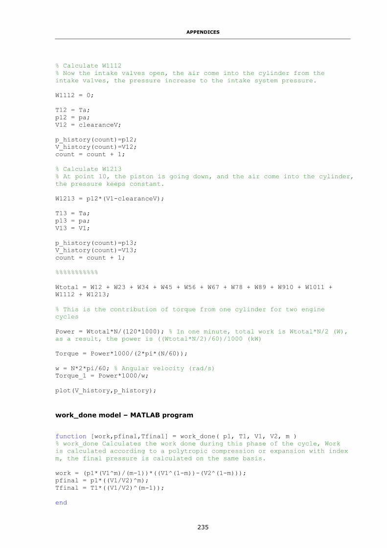
APPENDICES
235
% Calculate W1112
% Now the intake valves open, the air come into the cylinder from the
intake valves, the pressure increase to the intake system pressure.
W1112 = 0;
T12 = Ta;
p12 = pa;
V12 = clearanceV;
p_history(count)=p12;
V_history(count)=V12;
count = count + 1;
% Calculate W1213
% At point 10, the piston is going down, and the air come into the cylinder,
the pressure keeps constant.
W1213 = p12*(V1-clearanceV);
T13 = Ta;
p13 = pa;
V13 = V1;
p_history(count)=p13;
V_history(count)=V13;
count = count + 1;
%%%%%%%%%%%
Wtotal = W12 + W23 + W34 + W45 + W56 + W67 + W78 + W89 + W910 + W1011 +
W1112 + W1213;
% This is the contribution of torque from one cylinder for two engine
cycles
Power = Wtotal*N/(120*1000); % In one minute, total work is Wtotal*N/2 (W),
as a result, the power is ((Wtotal*N/2)/60)/1000 (kW)
Torque = Power*1000/(2*pi*(N/60));
w = N*2*pi/60; % Angular velocity (rad/s)
Torque_1 = Power*1000/w;
plot(V_history,p_history);
work_done model – MATLAB program
function [work,pfinal,Tfinal] = work_done( p1, T1, V1, V2, m )
% work_done Calculates the work done during this phase of the cycle, Work
is calculated according to a polytropic compression or expansion with index
m, the final pressure is calculated on the same basis.
work = (p1*(V1^m)/(m-1))*((V1^(1-m))-(V2^(1-m)));
pfinal = p1*((V1/V2)^m);
Tfinal = T1*((V1/V2)^(m-1));
end

APPENDICES
236
Appendix-II
Chapter 6 - GT-POWER model of the basic engine
A heavy-duty, six cylinders, turbocharged & intercooler diesel engine based on the
YUCHAI YC6A Series engine is used as the basic engine in this research. The pneumatic
hybrid systems are added to this engine to realize the different functions discussed in
Chapter 6 and 7. The GT-POWEER model of the basic YC6A engine is shown in Figure A-1.
The dimensions and characteristics of the basic engine GT-POWER model are shown in
Table A-1.
Figure A-1 GT-POWER model of the basic engine
Table A-1 Dimensions and characteristics of the basic engine GT-POWER model
Part Name Type Dimensions
Ambient-02, 350 Environment End
Pressure (bar) 1
Temperature (k) 298
comp_in01 Round Pipes
Diameter (mm) 101
Length (mm) 304

APPENDICES
237
comp_in02 Round Pipes
Diameter (mm) 84
Length (mm) 250
cooler-in-1 Round Pipes
Diameter (mm) 66.5
Length (mm) 55
cooler-1 Round Pipes
Diameter (mm) 5
Length (mm) 450
cooler-out-1 Round Pipes
Diameter (mm) 80
Length (mm) 550
803, 806 Round Pipes
Diameter (mm) 58.7
Length (mm) 34
802, 804 Round Pipes
Diameter (mm) 58.7
Length (mm) 66
801, 805 Round Pipes
Diameter (mm) 58.7
Length (mm) 132
7047, 7048,
7049, 7050, 7051, 7052
Round Pipes
Diameter (mm) 45.7
Length (mm) 57.4
P7015-1, P7015-
2, P7015-3, P7015-4, P7015-
5, P7015-6
Round Pipes
Diameter (mm) 45.7
Length (mm) 10
7058, 7060, 7062, 7064,
7066, 7068,
7057, 7059, 7061, 7063,
7065, 7067
Round Pipes
Diameter (mm) 32.4
Length (mm) 210
7662, 7664, 7666, 7668,
7670, 7672,
7661, 7663,
7665, 7667, 7669, 7671
Round Pipes
Diameter (mm) 37.8
Length (mm) 168.7
661, 664 Round Pipes
Diameter (mm) 40
Length (mm) 71
662, 663 Round Pipes
Diameter (mm) 40
Length (mm) 71
674, 675 Round Pipes Diameter (mm) 40
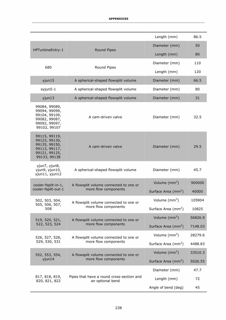
APPENDICES
238
Length (mm) 86.5
HPTurbineEntry-1 Round Pipes
Diameter (mm) 50
Length (mm) 80
680 Round Pipes
Diameter (mm) 110
Length (mm) 120
yjun15 A spherical-shaped flowsplit volume Diameter (mm) 66.5
syjun5-1 A spherical-shaped flowsplit volume Diameter (mm) 80
yjun13 A spherical-shaped flowsplit volume Diameter (mm) 31
99084, 99089,
99094, 99099,
99104, 99109, 99082, 99087,
99092, 99097,
99102, 99107
A cam-driven valve Diameter (mm) 32.5
99115, 99119,
99123, 99130,
99135, 99150,
99113, 99117, 99121, 99125,
99133, 99138
A cam-driven valve Diameter (mm) 29.5
yjun7, yjun8, yjun9, yjun10,
yjun11, yjun12
A spherical-shaped flowsplit volume Diameter (mm) 45.7
cooler-fsplit-in-1, cooler-fsplit-out-1
A flowsplit volume connected to one or more flow components
Volume (mm3) 900000
Surface Area (mm2) 40000
502, 503, 504, 505, 506, 507,
508
A flowsplit volume connected to one or
more flow components
Volume (mm3) 105904
Surface Area (mm2) 10825
519, 520, 521,
522, 523, 524
A flowsplit volume connected to one or
more flow components
Volume (mm3) 56826.9
Surface Area (mm2) 7148.03
526, 527, 528,
529, 530, 531
A flowsplit volume connected to one or
more flow components
Volume (mm3) 28279.6
Surface Area (mm2) 4488.83
552, 553, 554,
yjun14
A flowsplit volume connected to one or
more flow components
Volume (mm3) 33510.3
Surface Area (mm2) 5026.55
817, 818, 819,
820, 821, 822
Pipes that have a round cross-section and
an optional bend
Diameter (mm) 47.7
Length (mm) 72
Angle of bend (deg) 45

APPENDICES
239
256, 257, 258,
259, 260, 261
Pipes that have a round cross-section and
an optional bend
Diameter (mm) 37.8
Length (mm) 1403
Angle of bend (deg) 60
Furthermore, some important parameters are introduced here.
Discretization length
Based on the ‘Engine performance tutorials’ from GT-POWER, for general performance
analysis (Engine cycle simulation a discretization length of approximately 0.4 times the
cylinder bore diameter is recommended for the intake system and 0.55 times the bore is
recommended for the exhaust system. The difference in the recommendation for intake
and exhaust discretization is the result of differences in the speed of sound due to the
temperature. The bore diameter in this model is 105 mm, therefore the intake side
discretization length is 42 mm, and the exhaust side discretization length is 60 mm.
Cylinder Geometry
Table A-2 Cylinder Geometry
Bore (mm) 105
Stroke (mm) 132
Connecting rod length (mm) 210
Compression ratio (-) 17.5
TDC clearance height 1
Wrist pin to crank offset (mm) 0
Firing order
1-5-3-6-2-4
Intake and exhaust valves lift and timing
The intake valves lift and timing is shown in Figure A-2.

APPENDICES
240
Figure A-2 Intake valves lift and timing
The intake valves lift and timing is shown in Figure A-3.
Figure A-3 Exhaust valves lift and timing
Fuel injection system
The ‘Injection Profile Connection’ is used here as the fuel injector. This injection
connection allows for injection of a periodic mass flow rate or pressure profile. It may be
used to inject fluid into any cylinder, pipe, or flowsplit, but it is typically used for direct-
injection diesel engines. This template may be used with any cylinder combustion model.
The parameters of the nozzles are shown in Table A-2.

APPENDICES
241
Table A-3 Cylinder Geometry
Nozzle hold diameter (mm) 0.17
Number of holes per nozzle (-) 6
The introduction of how to run the GT-POWER and Simulink co-simulation
Any GT-POWER signals can be passed to or from Simulink via a 'SimulinkHarness'
component. There are two methods in which this can be accomplished:
(i) Running a GT-SUITE model from the Simulink interface.
(ii) Compiling Simulink model(s) into .dll/.so files and importing them into a GT-
SUITE model.
The advantage of the first method is that all the functions of MATLAB/Simulink can be
implemented. For example, the Global Optimisation Toolbox can be used to search for
global solutions to problems that contain multiple maxima or minima by running the
problem several times with different variables. For the second method, once the Simulink
model is compiled to the .dll/.so files, the parameters in the Simulink model cannot alter
any more. But in the first method, there is a restriction that only one ‘SimulinkHarness’
part may be used in the GT-SUITE model while the second method allows up to an
infinite number of ‘SimulinkHarness’ parts with the same or different imported Simulink
models. As the goal of this research is to develop the pneumatic hybrid city bus control
strategy, the optimisation will be one part of the develop process, as a result, the first
method has been chosen in this research.

APPENDICES
242
Appendix-III
In GT-POWER, the ‘DIWiebe’ model imposes the combustion burn rate for direct-injection,
compression-ignition engines using a three-term Wiebe function which is the
superposition of three normal Wiebe curves. These Wiebe curves approximate the
"typical" shape of a DI compression ignition, single main injection burn rate. The purpose
of using three functions is to make it possible to model the premixed and diffusion
portions of the combustion process.
The Wiebe equations are given below.
Constants calculation: Main Fraction (FM), Wiebe Premix Constant (WCP), Wiebe
Main Constant (WCM), Wiebe Tail Constant (WCT).
𝐹𝑀 = (1 − 𝐹𝑃 − 𝐹𝑇) (A-1) [90]
𝑊𝐶𝑃 = [𝐷𝑃
2.3021
(𝐸𝑃+1)⁄−0.015
1(𝐸𝑃+1)⁄
]
−(𝐸𝑃+1)
(A-2) [90]
𝑊𝐶𝑀 = [𝐷𝑀
2.3021
(𝐸𝑀+1)⁄−0.015
1(𝐸𝑀+1)⁄
]
−(𝐸𝑀+1)
(A-3) [90]
𝑊𝐶𝑇 = [𝐷𝑇
2.3021
(𝐸𝑇+1)⁄−0.015
1(𝐸𝑇+1)⁄
]
−(𝐸𝑇+1)
(A-4) [90]
where DP – premix duration,
DM – main duration,
DT – tail duration,
FP – premix fraction,
FT – tail fraction,
EP – premix exponent,
EM – main exponent,
ET – tail exponent.

APPENDICES
243
Burn Rate Calculation: the cumulative burn rate is calculated, normalized to 1.0.
The combustion starts at 0.0 (0.0% burned) and progresses to the value specified
by the "Fraction of Fuel Burned Attribute", which is typically 1.0 or 100%.
𝐶𝑜𝑚𝑏𝑢𝑠𝑡𝑖𝑜𝑛(𝜃) =
(𝐶𝐸)(𝐹𝑃) [1 − 𝑒−(𝑊𝐶𝑃)(𝜃−𝑆𝑂𝐼−𝐼𝐷)(𝐸𝑃+1)] +
(𝐶𝐸)(𝐹𝑀) [1 − 𝑒−(𝑊𝐶𝑀)(𝜃−𝑆𝑂𝐼−𝐼𝐷)(𝐸𝑀+1)] +
(𝐶𝐸)(𝐹𝑇) [1 − 𝑒−(𝑊𝐶𝑇)(𝜃−𝑆𝑂𝐼−𝐼𝐷)(𝐸𝑇+1)] (A-5) [90]
where θ – instantaneous Crank Angle,
CE – fraction of Fuel Burned (also known as "Combustion Efficiency"),
SOI – start of Injection, and
ID – ignition Delay.
‘WoschniGT’ model indicates that the in-cylinder heat transfer will be calculated by a
formula which closely emulates the classical Woschni correlation without swirl as detailed
described in [91]. This heat transfer model is used to define heat transfer characteristics
of the flow component in the engine model.

APPENDICES
244
Appendix-IV
Availability calculation:
Let V, T0, p0 be the air tank volume, environment temperature and pressure. Also, let a1,
u1, p1, T1 and m1 be the availability, internal energy, pressure, temperature and mass of
air tank at the initial point, and let a2, u2, p2, T2 and m2 be the availability, internal
energy, pressure, temperature and mass of air tank at the finish point, respectively (see
Figure A-4).
Figure A-4 Availability calculation
First, there are some assumptions should introduce before:
(i) Air is an ideal gas.
(ii) The kinetic and potential energies are negligible.
(iii) The properties of air at the environment remain constant during the entire
charging process.
If the air mass in the air tank is m1, the specific volume v1 is:
𝑣1 =𝑉
𝑚1 (A-6)
Since the temperature remains unchanged and
𝑝𝑣𝐴𝑇 = 𝑚𝑅𝑇 (A-7)
𝑣1 =𝑅𝑇0
𝑝1 (A-8)
Similar,
Initial
V, a1, u1, p1, T1
and m1
Finish
V, a2, u2, p2, T2
and m2
T0 T0

APPENDICES
245
𝑣2 =𝑅𝑇0
𝑝2 (A-9)
By definition:
𝑎1 = 𝑐𝑣𝑇0 − 𝑇0𝑆1 (A-10)
𝑎2 = 𝑐𝑣𝑇0 − 𝑇0𝑆2 (A-11)
And
𝑢1 = 𝑢2 = 𝑐𝑣𝑇0 (A-12)
𝐸 = 𝑚1𝑢1 − 𝑚2𝑢2 = 𝑚1𝑐𝑣𝑇0 − 𝑚2𝑐𝑣𝑇0 = Δ𝑚𝑐𝑣𝑇0 (A-13)
For availability
𝑇𝑑𝑠 = 𝑑𝑢 + 𝑣𝑑𝑝 (A-14)
Giving
Δ𝑆 = 𝑆2 − 𝑆1 = (𝑐𝑝 ln𝑇2
𝑇1− 𝑅 ln
𝑝2
𝑝1) = −𝑅 ln
𝑝2
𝑝1 (A-15)
So
Δ𝑎 = Δ𝑢 − 𝑇Δ𝑆 + 𝑝0(𝑣2 − 𝑣1) = 𝑅𝑇0(ln𝑝0
𝑝1+
𝑝1
𝑝0− 1) (A-16)
Finally, the availability change during the process can be presented
Δ𝐴 = 𝑚𝑅𝑇0(ln𝑝0
𝑝1+
𝑝1
𝑝0− 1) (A-17)

APPENDICES
246
Appendix-V
In the Generalized Pattern Search optimisation implemented at Chapter 4 and Chapter 7,
the fitness function and options of GPS is first input by using the Global Optimisation
Toolbox in MATLAB. Then the Global Optimisation Toolbox completes the pattern search
steps such as polling, expanding and contracting to implement the optimisation. All are
pattern search algorithms that compute a sequence of points that approach an optimal
point. At each step, the algorithm searches a set of points, called a mesh, around the
current point—the point computed at the previous step of the algorithm. The mesh is
formed by adding the current point to a scalar multiple of a set of vectors called a
pattern. If the pattern search algorithm finds a point in the mesh that improves the
objective function at the current point, the new point becomes the current point at the
next step of the algorithm [83]. The terminology of pattern search is shown as follows
[83].
Patterns - A pattern is a set of vectors {vi} that the pattern search algorithm uses to
determine which points to search at each iteration. The set {vi} is defined by the number
of independent variables in the objective function, N, and the positive basis set.
Meshes - At each step, pattern search searches a set of points, called a mesh, for a
point that improves the objective function. Pattern search forms the mesh by (i)
Generating a set of vectors {di} by multiplying each pattern vector vi by a scalar Δm. Δm
is called the mesh size, and (ii) Adding the {di} to the current point - the point with the
best objective function value found at the previous step.
Polling - At each step, the algorithm polls the points in the current mesh by computing
their objective function values.
Expanding and contracting - After polling, the algorithm changes the value of the
mesh size Δm. The default is to multiply Δm by 2 after a successful poll, and by 0.5 after
an unsuccessful poll.
Complete Poll - By setting Complete poll to On in Poll options can make the pattern
search poll the entire mesh. This is because for problems in which there are several local
minima, it is sometimes preferable to make the pattern search poll all the mesh points at

APPENDICES
247
each iteration and choose the one with the best objective function value. This enables the
pattern search to explore more points at each iteration and thereby potentially avoid a
local minimum that is not the global minimum. By default, if the pattern search finds a
mesh point that improves the value of the objective function, it stops the poll and sets
that point as the current point for the next iteration. When this occurs, some mesh points
might not get polled. Some of these unpolled points might have an objective function
value that is even lower than the first one the pattern search finds.