THE ASYMPTOTIC DISTRIBUTIONOF CERTAIN CHARACTERISTIC

ROOTS AND VECTORST. W. ANDERSONCOLUMBIA UNIVERSITY

1. IntroductionIn a number of problems in multivariate statistical analysis use is made of

characteristic roots and vectors of one sample covariance matrix in the metric ofanother. If A* and D* are the sample matrices, we are interested in the roots qb* ofD*- *A*1 = 0 and the associated vectors satisfying D*c* = O*A*c*. In

the cases we consider A* and D* have independent distributions. Each is dis-q

tributed like a sum yyay' where yi, . . ., yq are independently normally dis-a=

tributed with common covariance matrix. In the case of A* the means of the vec-tors are zero; in the case of D* the means may not be zero. We are interested inthe asymptotic distribution of the characteristic roots and vectors when the num-ber of vectors defining A* increases indefinitely and when the means of the vectorsdefining D* change in a certain way. The form of the limiting distribution de-pends on the multiplicity of the roots of a certain determinantal equation involvingthe parameters. If these roots are simple and different from zero, the asymptoticdistribution is joint normal. If the roots are not simple, the asymptotic distribu-tion is expressed in terms of "uniform distributions" on orthogonal matrices anda normal distribution.We shall first state our problem in a general form and show in what kinds of

statistical problems there is interest in these characteristic roots and vectors.Suppose' x.(a = 1, . . . , N) of p components is normally distributed independent-ly of x,s(a $4 #) with mean(1.1) gxc, = Bizia + B2z2aand covariance(1.2) (X.-,x.) (Xa- Ox.)where Zil and Z2a are vectors of fixed variates of qi and q2 components, respec-tively, and B1 and B2 are p X q, and p X q2 matrices, respectively..We shall usethe notation N(Blzla + B2Z2., 1) for the distribution of xa.

Most of the research contained in this paper was done while the author was Fellow of the JohnSimon Guggenheim Memorial Foundation (at the Institute of Mathematical Statistics, Univer-sity of Stockholm, and the Department of Applied Economics, University of Cambridge). Thework was sponsored in part by the Office of Naval Research.

1 Unless specifically indicated otherwise, a vector is a column vector; a prime indicates thetranspose of a vector or matrix. Vectors and matrices are indicated by bold face type.

103

I04 SECOND BERKELEY SYMPOSIUM: ANDERSON

On the basis of a sample (xl, z,l, Z21), ... (XN, Z1N, Z2N) the usual estimateof B = (BlB2) is

(1.3) B= ± xz'(~zaz:>',N

where Z = (ZlaZ2Q) and z zz is assumed to be nonsingular. The columnsa- 1

of B, say b,, are normally distributed with means ., the corresponding columnsof B, and covariance

(1.4) (b - ) (b.- Z vI

where ( ZaZa indicates the element of the inverse matrix in the u-th row

and v-th column.Let Qr- be the submatrix of(E ZaZa>1 consisting of the last q2 rows and q2

columns; this is also given byN N N-

(1.5) Q E ~Z/2az2 Y Z2al Z Z/.z) ZlaZ2a=l 2a1 la= I

a-1

Then (B2 - B2) Q(B2 - B2)' has a Wishart distribution with covariance matrix 2:and q2 degrees of freedom, denoted by W(X, q2). If q2 < p, this distribution, called

q2

singular, is the distribution of ) YuY where yu is distributed according tou 1

N(0, 1) independently of yv (u . v). The usual estimate of 2; isN N N

(1.6) A*= E (xa-Bza) (xa-Bza)'= Sxx -B z zaB'a=1= a=l

divided by N - (q, + q2). This matrix is distributed according to W(1,N -q- q2) independently of B.Many statistical problems, for example [3], [6], involve the roots of

(1.7) B2QB' - *A* =0 ,

or the vectors, for example [1], [2], satisfying(1.8) (B2QB'-qb*A*) c* =0

The p algebraically independent vectors c, satisfying (1.8) may be normalized by(1.9) c*A*C= n hX

where n = N - - q2 and 5gg = 1 and 5gh = 0 for g # h. We say that thesolutions of (1.7) and (1.8) are the "characteristic roots and vectors of B2QB2 inthe metric of A*." If we wish to test the hypothesis that the rank of B2 is r againstthe alternatives that it is greater than r we use the p - r smallest roots of (1.7).If we assume that the rank of B2 is r and we wish to estimate B2 (or, equivalently,

CHARACTERISTIC ROOTS AND VECTORS 105

estimate the linear restrictions on B2) we make use of the vectors c* satisfying(1.8) for the p - r smallest roots of (1.7).

In this paper we shall study the joint asymptotic distribution of the roots andvectors defined by (1.7), (1.8), and (1.9) when n = N - qi - q2-+ - and

zaz. approaches a nonsingular limit. The asymptotic distribution of then

roots alone has been given by Hsu [8]. We find it convenient to make use of someof the results in [81 to obtain the joint asymptotic distribution of roots and vectors;however, the method used in the present paper could be used independently of [8].We shall assume throughout the paper that q2 _ p.

2. Reduction of the problem to canonical form

To simplify the following derivations we shall transform the matrices B2QB2and A* so that they have distributions with fewer parameters. Corresponding to(1.7) and (1.8) in the sample, we have the population equations

(2.1) XB2QB2-r2Nj =0and

(2.2) (B2Q.B2-T2) = °

whereQn =-Q. Let the roots of (2.1) be Tl(n) _ rT(n) _ ... _ T(2(n) _ 0. Then 2

number of zero roots is the difference of p and the rank of B2 for each n for whichQn, is nonsingular (in particular for n sufficiently large). Let yi(n), ... , r'(n) be aset of corresponding solutions of (2.2) satisfying

(2.3) r, (n)X.Y(n) = -

Let rF = [y1(n), ... , y,(n)]. Then we can make a transformation, for example[7], so that A* is replaced by

(2.4) A. yo*y*g,where y,s is distributed according to N(O, I) independently of Y.* (, a), andB2QnB2 is replaced by

qt

(2.5) D. y** (n) y**'(n)0=1

where eg*(n) is distributed independently of y*h*(n) (g w- h) according to

N[RnTg(n)E,,, I] where Tg(n) is the nonnegative square root of r2(n) and zg is avector with all components 0 except the g-th (for g p) which is 1. The roots of(1.7) are the roots of

(2.6) ID.-,An =0 ,

and the vectors satisfying (1.8) and (1.7) are related to the vectors cl(n), . . . ,

cp(n) satisfying(2.7) (Dn-,A*) c =0

io6 SECOND BERKELEY SYMPOSIUM: ANDERSON

and(2.8) c'A ch = nf

by(2.9) c* (n) = rncg .

It should be observed that rn and Tr(n) depend on n because Qn depends on n.We shall first find the limiting distribution of cg(n) and Og(n) as nX (that

is, as N - ). Let yg = y*(n) - VnrT(n)Pg. Then

q2

(2.10) D. = [yg + VnTXrg,(n) 0][yg+ V\nTg(ne]'egg=1

and yg is distributed according to N(O, I).Let Cn = [ci(n), . . c(n)]. Then (2.7) can be written

(2.11) DnCn*= AnCn*n,where 4. = [bi(n)bij] and 41(n), . . .., 0(n) are the roots of (2.6) and (2.8) canbe written(2.12) C.ASCn= nI.

If(2.13) Xn =C,7lwe have

(2.14) -An =X'Xft,nn

1(2.15) -Dn =X4Xo -

We shall set out to find the limiting distribution of 4' and Xn for Tog(n) approach-ing limits as n -X a. To make 4n and Xn unique we require 41(n) > +2(n) > ...

> 4p,(n) and xii(n) > 0. The probability is 0 of a Dn and An for which X, and 4fnare not uniquely defined.

Throughout this paper we shall make use of the following special case of atheorem of Rubin [9]:

RUBIN's THEOREM: Let Fn(u) be the cumulative distribution function of a randomvector uf. Let Vn be a (vector valued) function of Unf Vn = fn(un), and let Gn(v) be the(induced) distribution of vn. Suppose lim Fn (u) = F (u ) [in every continuity point

n-* -

of F(u)] and supposefor every continuity point u of f(u), lim f. (unt) = f (u) , when

lim unt = u . Let G(v) be the distribution of the random vector v = f(u), where u has

the distribution F(u). If the probability of the set of discontinuities off(u) in terms ofF(u) is 0, then2

limG. (v) =G (v).n-* o

2 We could justify the limiting procedures by another method that consists of extending atheorem of L. C. Young ("Limits of Stieltjes integrals," Jour. London Math. Soc., Vol. 9 [1934], pp.119-126), concerning the limit of f9n(u)dFn(u), applying this to the characteristic function offn(Un), and thus obtaining a restricted for'm of Rubin's theorem.

CHARACTERISTIC ROOTS AND VECTORS I07

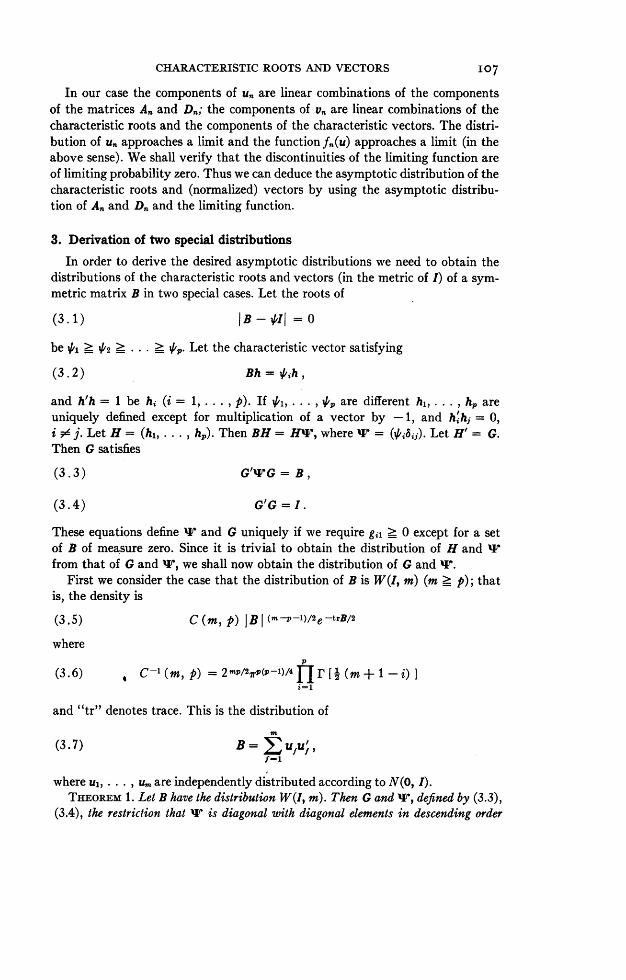
In our case the components of u. are linear combinations of the componentsof the matrices A, and Dn; the components of v,, are linear combinations of thecharacteristic roots and the components of the characteristic vectors. The distri-bution of un approaches a limit and the functionf"(u) approaches a limit (in theabove sense). We shall verify that the discontinuities of the limiting function areof limiting probability zero. Thus we can deduce the asymptotic distribution of thecharacteristic roots and (normalized) vectors by using the asymptotic distribu-tion of A, and Dn and the limiting function.

3. Derivation of two special distributionsIn order to derive the desired asymptotic distributions we need to obtain the

distributions of the characteristic roots and vectors (in the metric of I) of a sym-metric matrix B in two special cases. Let the roots of

(3.1) |B- &I =O

be {& >. 462 _ ... _ ',p. Let the characteristic vector satisfying

(3.2) Bh= Ch,and h'h = 1 be hi (i = 1, . . ., p). If ,1, ..,, are different hi, . h.,hp areuniquely defined except for multiplication of a vector by -1, and h'h = 0,i F- j. Let H = (h1, ... , h,). Then BH = HW, where v = (4X6ij). Let H' = G.Then G satisfies

(3.3) G'WG= B,

(3.4) G'G =I.These equations define v and G uniquely if we require gil > 0 except for a setof B of measure zero. Since it is trivial to obtain the distribution of H and vfrom that of G and ', we shall now obtain the distribution of G and W.

First we consider the case that the distribution of B is W(I, m) (m _ p); thatis, the density is

(3.5) C(m, p) B (m-pl)/2e-trB/2

wherep

(3.6) C-1 (m, p) = 2mP/27rp(p-1)/4rJIr [a (m+ 1-i)]i=l1

and "tr" denotes trace. This is the distribution of

(3.7) B UfUff-i

where ul, ... , u,- are independently distributed according to N(O, I).THEOREM 1. Let B have the distribution W(I, m). Then G and IF, defined by (3.3),

(3.4), the restriction that W is diagonal with diagonal elements in descending order

io8 SECOND BERKELEY SYMPOSIUM: ANDERSON

and gil > 0, are independently distributed. The density of the diagonal elements ofv is

(3.8) 1p/(-1)/2e- Oi/2

2pm/2 Jr[I (m+1-i)Ir[FL(p+1-i)] I

P P

X rI r (4,i CA)i=l j=i+l

for f, > . . .> 4p > 0 and is 0 elsewhere. The distribution of G is "uniform."PROOF. That the marginal density of 4,1, ..., 4p is (3.8) has been proved by

Hsu [5]. It remains to show that G is distributed independently of v and "uni-formly." The "uniform" distribution of all orthogonal p-dimensional matrices isgiven by the (normalized) Haar measure on the orthogonal group; that is, the(normalized) Haar measure is the only probability measure on the group that isinvariant under the group operation on the right [4]. Since we require gil > 0,our definition of "uniform distribution" is the conditional distribution obtainedfrom the Haar measure by requiring gil _ 0. For this part of the space the prob-ability measure is 2P times the normalized Haar measure.

The measure on the space of uf defines a measure on the space of G, gil > 0.Consider any measurable set H in the space of all orthogonal matrices. Let thediagonal matrices with diagonal elements + 1 and - 1 be J1, . . . , J2P. Let H

2PE Hi, where JiHi is a set in the space of G, gil > 0. Define the measure of H asi=l1

the sum of the measures of JiHi. Now let us show that this measure is invariantwith respect to multiplication on the right. Let Ei be the set in the space of ufthat maps into JiHi. Let H* be HP; that is, H* is the set obtained by multiply-ing each element of H on the right by the orthogonal matrix P. Then H*=

H*= z HIP. We now show that the measure of H* is the same as Hi. Let

H* =! H!. such that J1H*1 is in the space gil > 0. Let E*ij be the set in the

space Uf that maps into JiH',. Then E!.=P'Ei; that is, SEI. is the seti i

obtained by multiplying each (ul, . . ., u,) by P' on the left. The measure ofP'E, is the integral of the density of P'ul, . . ., P'um over Ei. Since the densityof P'ul, . . . , P'u,,, is the same as that of ul, . . . , ur, the measure of P'E, isthat of Es. Thus the measure of H* is that of H. This proves that the measure isinvariant with regard to the group operation on the right. Since there is only onesuch measure on the group of orthogonal matrices with total measure 2P, this is it.The joint distribution of 0 and G(gii _ 0) has a density. This density does notdepend on G because the density at 4 and G is the same as at 4' and G* since G*can be obtained from G by multiplication on the right by some orthogonal matrix Pand this is equivalent to transforming B to P'BP which has the same characteristicroots as B. This proves the theorem.Now suppose the density function of B = B' is

(3.9) .7r ~~~-P(P+1)/42 -p/2e-trB2/2

CHARACTERISTIC ROOTS AND VECTORS IO9

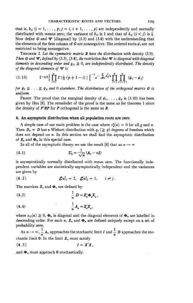
that is, bij (i = 1, . . ., p; j = i, i + 1, . . . , p) are independently and normallydistributed with means zero; the variance of bi is 1 and that of bij (i < j) is -.Now define G and W (diagonal) by (3.3) and (3.4) with the understanding thatthe elements of the first column of G are nonnegative. The ordered roots ,t' are notrestricted to being nonnegative.

THEOREm 2. Let the symmetric matrix B have the distribution with density (3.9).Then G and Mr, defined by (3.3), (3.4), the restriction that vis diagonal with diagonalelements in descending order and gil > 0, are independently distributed. The densityof the diagonal elements of W is

(3.10) 2-p/2j [2 p -)] Pei/2-ly (+_+i=l ~~~~~~~~i=l=+

for 4t1 _ ..._ p and 0 elsewhere. The distribution of the orthogonal matrix G isuniform.

PROOF. The proof that the marginal density of ', ... , p is (3.10) has beengiven by Hsu [8]. The remainder of the proof is the same as for theorem 1 sincethe density of P'BP for P orthogonal is the same as B.

4. An asymptotic distribution when all population roots are zero

A simple case of our main problem is the case where Tr(n) = 0 for all g and n.Then Dn = D has a Wishart distribution with q2 ( p) degrees of freedom whichdoes not depend on n. In this section we shall find the asymptotic distributionof X. and 4bn in this special case.

In all of the asymptotic theory we use the result [8] that as n -+ o

(4.1) U.n= (A. -nl)

is asymptotically normally distributed with mean zero. The functionally inde-pendent variables are statistically asymptotically independent and the variancesare given by(4.2) Cui = 2, gui, = 1, i j.

The matrices Xn and 4On are defined by1

(4.3) -D =X4'Xn.n

1(4.4) -A. =X'X,,

n

where xii(n) _ 0, On is diagonal and the diagonal elements of 4', are labelled indescending order. For each n, Xn and 4', are defined uniquely except on a set ofprobability zero.

1 1As n ,- An approaches the stochastic limit I and - D approaches the sto-n n

chastic limit 0. In the limit Xn must satisfy(4.5) I = X'X,

and ,n must approach 0 stochastically.

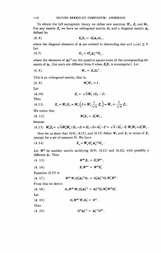
IIO SECOND BERKELEY SYMPOSIUM: ANDERSON

To obtain the full asymptotic theory we define new matrices Wn, Zn and 0e.For any matrix X, we have an orthogonal matrix °n and a diagonal matrix Andefined by(4.6) X Xn = O.AnOn,where the diagonal elements of A are ordered in descending size and o?,(n) > 0.Let(4.7) G.= °OA/20

where the elements of an/2 are the positive square roots of the corresponding ele-ments of An (the roots are different from 0 when XnXn is nonsingular). Let

(4.8) Wn = XnG[-1 .

This is an orthogonal matrix; that is,

(4.9) W, Wn = I

Let

(4.10) Zn ViWn(Gn-I) .

Then

(4.11) Xn WnGn= Wn(I+ Wn Zn) = Wn+ Z. -

We notice that

(4.12) WnZ = Zn Wn.because

(4.13) W,ZnZ VWnWn (G n-I) = Gn-I= Gn-It= / (Gn-I) WnWnZnWn-

Now let us show that (4.9), (4.11), and (4.12) define Wn and Zn in terms of Xn(except for a set of measure 0). We have

(4.14) Xn=W AOnan/2OnLet W* be another matrix satisfying (4.9), (4.11) and (4.12), with possibly adifferent Zn. Then

(4.15) W* Xn = XnW

(4.16) XnW* = W*XEquation (4.15) is

(4.17) W*/WnO AOj2On = On,n/2OnWnW*From this we derive

(4.18) OnW* WnO,Ai/2 - A/2OnW.'W*O.'Let

(4.19) OnW* WnOn = 0*

Then

(4.20) O*ni/2= an/20*'.

CHARACTERISTIC ROOTS AND VECTORS III

The component equations are

(4.21) -=

This gives us1/2

(4.22) 1/2 °i-

From (4.16) we derive61/2

(4.23) _0i

If Si 5d Sj, o*'j = 0. Therefore, if the bi are all different

(4.24) 0* = I,and

(4.25) W*= W.

Therefore, except for a set of measure zero of X,,, (4.9), (4.11), and (4.12) defineW,, and Zn uniquely. Let

(4. 26) 0n=fl4nn-

Now let us substitute into (4.3) and (4.4). We obtain

(4.2 7) D = W.nOWn+ i (ZnOnWn + WnOnZn) + ZnOnZn,/n- n

(4.28) Un=W.Zn+Z'Wn+ T;ZnZn.

Together with (4.9), (4.12) and

(4.29) wil (n) + zil (n) _ 0, i= , . . .,

(4.27) and (4.28) define 0n, Wn and Zn uniquely for each n.For given W,, = W, Zn = Z and En = 0 the limits of (4.27) and (4.28) ex-

pressing D and U in terms of Wn, Zh and En are

(4.30) D = W'OW,

(4.31) U= W'Z+ Z'W = 2W'Z.

If

(4.32) wil_O,

and Es > Oj for i > j, then (4.9), (4.12), (4.30) and (4.31) define W, Z, and 0uniquely in terms of D and U (except for a set of D and U of measure 0). Nowwe wish to argue that if we take (4.9), (4.12), (4.27), (4.28), and (4.29) as de-fining Wn, (diagonal) On, Zn in terms of (nonrandom) D = Dn and Un, the limitof Wn, O,n and Zn is the solution of (4.9), (4.12), (4.30), (4.31), and (4.32) asn -k - for Dn -* D and U,, -4 U where D and U are such that the solution is

II2 SECOND BERKELEY SYMPOSIUM: ANDERSON

unique (the exceptional D and U are of measure 0). A diagonal element of 0n is aroot of

(4.33) Dn- 9(I+ IUn) =0.As n x, this root approaches the root of

(4.34) ID- OI| = 0,

and this is an element of 0 defined by (4.9) and (4.30). Z,n is defined (equivalently)by(4.3 5) Zn.= Vn(Xn-Wn) =Xn. V°n (IA)-An On,

where the diagonal elements of An are roots of

(4.36) v-Un +I- ail =0.Let 4'i(n) be the i-th root of

(4.37) |Un 0-I=0.Then

(4.3 8) bi (n) =I1+ i(n).Clearly

(4.3 9) lim -V [ 1- e-/2 (n) ] =alim#1i (n) =4,ji.

Since XnXn --+I and On is orthogonal, each element of Zn is bounded in the limit.1, 1 'nWThus the norm (any standard norm) of a ZnZn and the norm of \i (Z.EnWn +

W,e0nZn) +-Zn0nZn go to zero as n . Thus each element of Dn-W nWn

and each element of Un - 2WnZn goes to 0 as n - . Consider the matrix function(P, Q) = (D - W*`0*W*, U - 2W*'Z*), where W* and 0* satisfy our usual condi-tions including (4.32). The inverse functions W*, 0*, Z* (as functions of P and Q)are continuous in the proper domain (except on the exceptional set). Hence, if thenorm of (P, Q) is sufficiently small the norm of (W* - W, 0* - 0, Z*- Z)must be arbitrarily small. If wil > 0, then wel > 0 for norm of (P, Q) sufficientlysmall. Then wil(n) for n sufficiently large is bounded away from 0, and for n suffi-ciently large wii(n) satisfying (4.29) must satisfy (4.32). Thus Wn, On and Zn con-verge to W, 0, and Z defined by (4.30) and (4.31).

The limiting equations (4.30) and (4.31) define W, Z, and 0 uniquely excepton a set of Lebesgue measure zero. The discontinuities can only occur on this set.Now considering D and Un as random matrices we observe that the limiting distri-bution of D and U. is absolutely continuous. Thus the conditions of Rubin'stheorem are fulfilled. To obtain the limiting distribution of the random matricesWn, Zn and On defined in terms of the random matrices D and Un we need onlyfind the distribution of W, Z and 0 defined by (4.9), (4.12), (4.30), (4.31) and(4.32), where U has the limiting distribution of Un.The distribution of W and 0 is that of theorem 1. The conditional distribution

CHARACTERISTIC ROOTS AND VECTORS II3of Z given W and 0 is obtained from(4.40) Z= WU.

Thus(4.41) g{zIW} = 2Wg2 =O .

Let(4.42) U= (ui,. . .u)

Z= (Z1,* , Zp),W = (W1,. , W..).

Then

(4.43) gt zizi I WI =41 We(C* )wW.

Since guWi = 2 and Wi4j = 1 for i #]j, and tuiJUkl = 0 otherwise, then

(4.44) I+ rii,

guuiU =£j

where ei, is a matrix with 1 in the i-th row and j-th column and O's elsewhere.Thus

(4.45) -IzizXI W) = 4w(Ibij+ £ji)W/= XVa ij + wjW') .

Since U is normally distributed, the conditional distribution of Z is normal.THEOREm 3. Let D have the distribution W(I, q2), q2 _ p, and let A,, be inde-

pendent of D, and have the distribution W(I, n). Define X,, and 4,, by means of (4.3),(4.4) and the conditions that xii(n) _ 0 and 4'n is diagonal with diagonal elements

1in descending order. Let n4b,, = 0, and let X,, = W, + VS; Z,, where W, W,, = Iand W,Z. = ZtW,,. The limiting distribution of 0, W,, and Z,, as n-aoz is thejoint distribution of 0, W, and Z such that the marginal distribution of the diagonalmatrix 0 and the orthogonal matrix W is that of theorem 1 with m = q2 and the con-ditional distribution of Z given W and 0 is normal with mean 0 and covariancesgiven by (4.45).

5. An asymptotic distribution when all population roots are equal but differ-ent from zero

Another special case that is easy to treat is the case of all roots of (2.1) beingequal but different from 0, say, Tr2(n) = ... = T2(n) = ,, > 0. Then

(5 .1) Dn = F+ -VnEn+ n AnI Xwhere

q2

(5.2) F = Y0yg,g-1

and E,, is composed of elements

(5.3) d n ii+ Yii) -

I14 SECOND BERKELEY SYMPOSIUM: ANDERSON

We are interested in Xn and 4'n (diagonal) defined by1 1

(5.4) 1 F+ aE.+ XnI =XninOn

1(5.5) -A. =Xn'X7n

with xii(n) _ 0 and the diagonal elements of On arranged in descending order.Let

(5.6) X. = Wn+ Zn,

where W,, and Z, satisfy (4.9) and (4.12). Let

(5.7) O n

where 0n is diagonal. Then (5.4) and (5.5) are

(5.8) -F+ 1En+ X.I= W"+ Zn) (I+ 0.)(Wn+ Z.)

n / n nn+ nn+ eW]

+ n[W.0Zn + ZnOnWn +)nZZnn + W3/2 Zn nZnI

(5.9) -A.(Wn+ Z.)' (Wn++ Zn);that is,(5.10) -; (A -nI) = (WKZ,+Z,W,) +-7,ZnZn

Multiply (5.10) by Xn and subtract from v/n times (5.8) to obtain

(5.11) 4FF+En- I. X. (A. -fnI) =W.ZnWn+T 4+[WnenZn+ZWnI+ Z., 19 Zn

Let

(5.12) U. = -4= (An- nI)-

Then (5.10) and (5.11) can be written as

(5.13) Un = (WZ,+ ZnW, +

(5.14) ZWF+E.-kU.=WKOW,+ v/H[W.lO +Z ,OnWn] +- Z.0,Z ,

where(5.15) W, W, = I,

(5.1 6) Wn'Z_ = Z.'Wn

CHARACTERISTIC ROOTS AND VECTORS II5

(5.1 7) w1l (n) + zi (n . .

Thus for a given n, 0,, W,, and Z,, are defined as functions of U., F = Fn and En.The functions are unique and continuous except over a set of U,, Fn and En ofmeasure zero. The limit of the functions (as U,, -+ U, F,, -n F, and E,, -n E) is thesolution to

(5.18) U= W'Z+ Z'W = 2W'Z,

(5.19) E - XU=W'OW,with W satisfying (4.32) and where X = lim X,,. This argument is justified as in

section 3. In particular, each diagonal element of 0,, as a function of nonrandomF,, E,, and U,, is a root of

(5.20) F.F +E.+ -\nX1- (U. + V/iO 0. + \In 0)| =°'

that is, of(5.21) ( A F. +En- x,un) (I+ - U.) -oI = °.

Since

(5.22) (-=Fn +En -XnUn)(I+ 8/iUn.)-+E-XU,the ordered roots of (5.20) approach the ordered roots of

(5.23) jE - XU -OIj = 0.

As in section 4 we can argue that the elements of W., O,, and Zn are boundedfor F, -n F, E,, -n E and U,, -÷ U. Then the elements in (5.13) and (5.14) whichare multiplied by 1/v4i, l/n and 1/n3/2 go to zero. The remainder of the argumentof section 4 applies.We can now use Rubin's theorem since the discontinuities of the mapping oc-

cur where there is indeterminacy and the set of E and U where this occurs is oflimiting probability 0. To find the limiting distribution of the random matricesW,,, 0,,, and Z,, we need only consider the distribution of the random matrices W,0, and Z defined by (5.18), (5.19) and (4.32) (with Worthogonal, 0 diagonal withdiagonal elements in descending order), where the random matrices E and U havethe limiting distribution of E,, and U.. Let

(5.24) E -XU = V.The density of E and U is(5.25) k e trE2/(4x) +trU2/2)/2 = ke-tr( (V+X U)I+2 U)A/(8X)

= ke -trl VI+2?XUV+XU2P+2XU2 /(8X)

= ke-tr( (X2 + 2X) ( U+ [/(X2+ 2A) V) I + [ 2A/(A 2+ 2X) I VI) /(8 )

= ke -(X+2)tr(U+[1/(X+2)]V)2/8e-trV/(4XI+8X)

This marginal density of V is normal, and the conditional density of U is normal.The distribution of W and (2X2 + 4X)-1/20 is that of theorem 2. The conditional

ii6 SECOND BERKELEY SYMPOSIUM: ANDERSON

distribution of Z given W and 0 is normal with mean

(5.26) g{ZI W, e}=JWC{UJ W, e}=w(-x+2 V)=-2(X+2) eW-

The conditional covariance between two columns of Z is(5.27) Ct [zi-t(zijW, 0)][zj-c(zjlW, @)]'W, e}

=W(ui+2+; Vi)(Uj+2+X Vj) IV{W,2 >- 4(Ibij+Wii).

TIHEOREM 4. Letq2

(5.2 8) Dn= (Yg + nVX to) (Ye + VnN/VnCg)

where the p-dimensional vectors yi, . .y,y2 (q2 > p) are independently distributedaccording to N(O, I); let An be independently distributed according to W(I, n). De-fine Xn and 0. by means of (4.3), (4.4), and the conditions that xil(n) > 0 and 4bn isdiagonal with diagonal elements in descending order. Let On = v;(4,n- XnI) and

X.= W. +1

Z,, where WIW. = 1, and W,Z,, = WWn. The limiting distribu-tion of O,,, Wn and Zn as n -- o is the joint distribution of 0, W and Z such thatthe marginal distribution of (2X2 + 4X)-1/2 times the diagonal elements of the diagonalmatrix 0 and the orthogonal matrix W is that of theorem 2 and the conditional distri-bution of Z given W and 0 is normal with mean (5.26) and covariances (5.27).

6. An asymptotic distribution in the general case

Now we consider the general case of the population roots having different values.We assume that the multiplicities do not depend on n, but the values may. Let

(6.1) [r2 (n) b,j] = fAi(n)I 0 0O10 X2 (n)I ..... o 0

o o .... Xh(n)Io01 o 0 .... 0 o

An,h

say, where Xi(n)I is of order ri and rh+1 = p - ri is the multiplicity of 0. Par-i-i

tition X", F, En and U. similarly, to [rT(n)5i,I. Let(6.2) X r(Win) 0 .... 0 1 'Zl(n) Z12(n) ... Zlh+l

0 W2 (n) .... 0 "'i Z21 (n) Z22 (n) ... Z2,h+l |

0 0 .; . . 1V+l(n) (Zh+l.l Zh+1,2 ... Zh+l,h+lJ

=Wn,+ -Zn

CHARACTERISTIC ROOTS AND VECTORS II7where

(6.3) Wi(n)Z,i(n) = Zii(n)Wi(n).

As before, this defines Wi(n) and Zii(n) uniquely in terms of Xii(n). To make X,unique in this case we now require that the elements of the first column of Xi(n)be nonnegative.

Let

(6.4)

4= XI(n)I+,01(n) 0 ... 0 0

0 X2 (n)I+7=02(n)... 0 0

o o .. Xh (n)I+-4=0h (n) 0O O *-- ° n eh+l(ff) .\/n0 0 .. 0- h1n

Then

(6.5) -D. =-F±F+ -;En+ A=X,,4,X, .

I 1-(6.6) -A,= U .+I=XtXn.

The submatric equations of (6.6) are

(6.7) Uii (n) +I = zXi (n)Xji (n)

= W.(n) W (n) + 4-[Wi(n)Zii(n) + Zii(n) Wi(n)]

+ n Zji (n) Zji (n) .

(6.8) Ui, (n) = X,i(n)Xkj(n)

=/[W'(n)Zij(n) +Zji (n) Wj (n)]

+ - Z;i (n) Zkj (n), i j

The submatric equations of (6.5) are

I Ic(6-9) n Fij+ n=Eii (n) + Xi (n)I= 1: X;i (n) 4k (n) Xki (X)

nVn= k~V=X (n)kiWi(n)W+ + Zki(n))(k (n)I+0Ok (n)X

X( kiWi (n) + ,/ Zi n) + nii Zh+l,i (n) 0h+1 (n) Zh+,,i (n)

XiW(n) Wi (n) Wi (n) + W,,'W(n) 0 iWi (n) + Xi (n) X

II8 SECOND BERKELEY SYMPOSIUM: ANDERSON

X [W. (n)Z.i(n) +Zii(n)Wi(n)]}+n[ Xk(n)Zki(n)Zki(n)

k-i~~~~~~~~~-+ W. (n) e i (n) Zii (n) +Zii (n) 0 i (n) Wi (n) I

+ n3/2 Zki (n) Ok (n)Zki (nt) + n-24+l i (n) Oh+l (n) z;+lA'zn) X

1~~~-

(6.10) -Fh+l,h+l =X,h+1(n) bk (n)Xk,h+1 (n)n ~~~~k

h~~~~~~~~~~~

= -[FZk,h+l (n) (\k (n) I+ Ok (n) ) Z;,h+l (n) + (Wh+i (n)

+ 4aZ+lsh+l (n) )Oh+l (n) (wh+l (n) + Zh+l,h+l (n) )

=-[Wh+1 (n) Oh+l (n) Wh+l (n) +I Xk (n) Z;,h+l (n) Zk,h+l (n)]

+3/2 [ ZkIh+l(n) 0k(n)Zk,h+l(n) + Wh+l('n) h+l(n)Zh+l,h+l(n)

+ZA+1,h+I(n) eh+I (n) Wh+1(fn)] 1'+,h+l(n) Oh+l(n)Zh+l,h+l(f)

(6.11) -Fij+ Eij (n) = X (n)4k (n)XkJ(n)

= ,(jkiWi(fl)+74Zkt(f))(\xk(flI 1\=e()

x(5k,Wj(n) + ;v ZkJ(n) )+n-2Zk+l.ifl() Oth+l (n) ZA+l,, (n)

=-\; LX. (n) 1V(n)Zij(n) + X1(n)Zi (n) W,(n) ]

+n[xk(n)zinZkJn +W(n) k (n)Zij(n)+Z;(n)0,(n)

1 1 1k

(6.12) - Fi,h+1 +-=Ei,h +1 (n) = zXXi(n) 4>k (n)Xk,h+i (nf)

= e( iWik(n)+iWn)Zk+(n))(Xk (n)I+ -k=Wk(n)O) nZk)h+x(n) +

k-- i

CHARACTERISTIC ROOTS AND VECTORS II9

+ - Zh+1,i(n)! Oh+(n)(Wh+1(n) + Zh+l,h+l(n)

= 1n Xi(n)Ws(n)Zi,h+l(n) +±[[W$(n)Oi(n)Zi,h+l(n) + z X,(n)n ~~~~~~~k-i

X Zki (n) Zk,h+ I (n)]+ 3/-2 [ EZki (n)ok (n) Zk,h+ 1(n) + Zh+1,i (n)k=i

x eh+l (n) Wh+ l(n) ]+ n2 Zh+l,,i (n)0h+l (n) Zh+l,h+l (n), i5- h + 1

For fixed F, En = E and Un = U (in the proper domain) the above equationsdefine the orthogonal Wi(n), Zi(n) and the diagonal 0i(n) uniquely (except for aset F, E and U of measure zero) under the restrictions that the elements in the

first column of Wi (n) + - Zii (n) are nonnegative and that the diagonal ele-

ments of the Oi(n) are in descending order. Now subtract I from each side of (6.7)and Xi(n)I from each side of (6.9) and multiply (6.7), (6.8), (6.9), (6.11) and(6.12) by -Fn and (6.10) by n and let n -* c. Using the fact that Wi(n) is orthogo-nal and (6.3), we obtain the limiting equations [for Xj(n) -1 Xi, E- E, andUn - U](6.13) Uii = 2 WiZii,

(6.14) Uij= wizii+zXiiw, i#j,(6.15) Eii -= wiiwi + 2XiWiZii h + 1,

h

(6.16) Fh+l,h+l =WA+10h+Wh+l+ XkZk,h+lZk,h+l,k=1

(6.17) Ei; = XiW:Zij + ,Z,iWj, i $ j; i, j 9 h+ 1,

(6.18) Ei,h+l = XiWiZi,h+l, i h + 1.

From (6.13) and (6.15) we obtain(6.19) Eii-XiUii= Wi'iWi.From (6.16) and (6.18) we obtain

(6.20) Fh+ls h+1 Ei,h+lEi,h+l = Wh+10h+Nh+lXi

Then the fact that Wi is orthogonal and the requirement that the elements of thefirst column of Wi be nonnegative define Wi, Zij, and 0i uniquely.

To show that Wi, Zij, and 0i defined by (6.13), (6.14), (6.17), (6.18), (6.19)and (6.20) are the limits of the matrices defined by (6.7)-(6.12) is more compli-cated than the similar demonstration in section 4. We shall only sketch this proofbriefly. First we should like to prove that the diagonal elements of 01(n), for

I20 SECOND BERKELEY SYMPOSIUM: ANDERSON

example, converge to the characteristic roots of El, - X1U11 as F,, -n F, En-- Eand U,, -> U. From the equation

(6.21) |F.+±-= En+± An-¢' (--=U+±I)| =0in Vnfl \VW

we can show that the first r, elements of 4p,, converge to Xl. Then we need to showthat the largest root of (6.21) minus Xl(n) times /n converges to the largest char-acteristic root of El, - XlU1j. That can be argued from the determinantal equa-tion

1 1

(6.2 2) -F. + En+ A.n-( U +I)(X1(n)I+ =I)|= F±+ 1 [En-Xl(n)Uj +(A.Xl (nI)- 0( 1Un+I)1=0.

In the second determinant above we can factor out oVn from the first ri rows.Then as n -* o there are r, sequences of roots each of which converges to a char-acteristic root of E1 - XUui. Similar arguments suffice for El(n) (i F4 h + 1).For 0h+l(n) we can use a slightly more complicated demonstration.3

Next we wish to argue that the elements of Zij(n) are bounded as n - (asF. -+ F, E. -n E, and U. - U). For convenience let us take the case of ri = 1.Then the characteristic vector say cl(n) associated with the largest root 01 satisfies

(6. 2 3) [-F.+ -[En- Xi (n)U.]+ [An- Xi (n)I]- = , ( = U,,+I)] c= O-

Then the components of cl(n) are

(6.24) cil (n) =k (n) rjt [ 7r2 (n)-Xi (n) ]+ -,ki (n) ]

(6.25) c(i (n) = k (n) ki (n),

where k(n) approaches a finite limit and ki(n) are bounded. Using the same rea-soning for each characteristic vector (assuming ri = 1) we show that C. is adiagonal matrix with bounded elements plus 1/Viz times a matrix with boundedelements. Thus X, = C;7 is of the same form. Therefore, Vnxij(n) = z;j(n)(i 0 j) are bounded. From

(6.26) n i (n) + I = xi (n)

= XL (n) +E X2, (n)ioi

we see that /[l - x2ii(n)] =-uii(n) + vix2ij(n) is bounded. Thus zii(n) =V-n[l - xii(n)] is also bounded. If ri # 1, essentially the same argument can becarried out in terms of the partitioned matrices. Thus the norms of matrices suchas Uii(n) - 2W1'(n)Z1j(n) go to zero. The argument of section 4 shows that Zii(n)approaches Zii, etc.

Since these arguments are similar to Hsu's [81, it is unnecessary to go into more detail.

ChIARACTERISTIC ROOTS AND VECTORS 12I

We are now in a position to apply Rubin's theorem. The discontinuities occurwhere W, Z, and 0 are not defined uniquely and the measure of U, F and E wherethis occurs is zero. Let the limiting distribution of the random matrices Un, F,and E,, be the distribution of the random matrices U, F, and E. Then the limitingdistribution of the random matrices W. (orthogonal diagonal blocks), Z,, and 0E(diagonal) defined by (6.7)-(6.12) is the distribution of W (orthogonal diagonalblocks) Z, and 0 (diagonal) defined in terms of the random matrices U, F, and E by(6.13), (6.14), (6.17)-(6.20). The distribution of Eii - XiUi, i F6 h + 1, is thatof section 5. Hence, the distribution of Wi and Oi is that given there. SinceEii- X1iUii is independent of Ejj- XjUj,, i # j, the matrices Wi and 1i, i = 1, ....h are independent. The conditional distribution of Zii given Wi is also that of sec-tion 5 with X = Xi, 0 = Oi, W = Wi and p = ri-

Now, consider (6.20). An element of Ej,h±j is egk = '/Xiyk, (ri + **. + ri_- +< g r + ...+ ri; p-rh+1+ 1 < k _P); an element of Fh+1,h±+ is

92 h 1 q2

fkk' = YkYkY', Thus an element of Fh+1,h+-I X Ei,h+lEi,h+l isS Ykgyk'g0=1~~~~~~ ~ ~~~i=

E=

p-rh+ 1 g2

- ) ykgYk'o = YYkoykY' . This matrix of order, r7h+ has the distributiong=l g `ho +1

W(I, q2 - p + rh+1) and is independent of Eii, i h + 1, and Eij, i Pd j. Thedistribution of Wh+±, Oh+, and Zh+,,h+l is that of section 4 with W = WA+1, 0 =0h+1, Z = Zh+l,h+l, P = rh+l and m = q2 - p + rh+1i

The matrices Uij and Eij, i 0 j, are independent of the other submatrices (ex-cept E,i = Ei' and Uji = Uij). From (6.14) and (6.17) or (6.18), we obtain

(6.27) Eij- XjUij= (Xi- X)WiZij.

The conditional distribution of Zij given Wi is that of

(6.28) X - Wi (Ei - XjU1i) .

An element of Ei1 is

(6.29) egf V/X1y1f+ VXiyf , r+. . .+ r-+ 1 g ri+... + ri,

Thus an element of Eij - XjUij is normally distributed independently of the otherelements with zero mean and variance Xi + Xj + X)2. The conditional distributionof Zij given Wi is normal with mean 0 and covariance between two elements is

1 i(6.30) gtz{f zg1f WIWi2= (ekf - XJUkf)wgk(ek1f- XjUk'f')

=(X- X) 2 WokUQk' 8ff' 5kk' (Xi + Xk+ X )

Aff~~~' (°°;(++j+jX2))

Thus the variance of zgf is (Xi + Xi + X2)/(Xi - Xj)2 and the covariances are zero.

122 SECOND BERKELEY SYMPOSIUM: ANDERSON

The conditional distribution of Zji is similar except that i and j are interchanged.Zij and Zji are independent of the other matrices. Now consider the conditionalcovariance between an element zf1 of Zij and zXof' of Zji. It is

(6.3 1) g t zfZ0 'f ' | Wi, W, } = (X - X) 2 k,kWOk (ekf - XiUkf)

XWgIk (ef'k'- XiUf'k')

Xi+ Xj+ 2ixj wW(y) Ij(1ii-Xj) gWk WO k Skf' Sfk'(Xi xj) ~k,k'

+ +fWg( f -

We can indicate the conditional covariances between the columns Z=(z1, . .. , z,) in matrix form. If g, f _ r1, the conditional covariance between z.and zf is(6.32) gzz,z , WI=

TX + 4(IC°f+i)W )' . .. o

o ~~~~Xi+X2+. .° (Xl - X2)

IB6of ..

*

O O X'1 I Sof.If g _ ri and r1 + 1 _ f _ ri + r2, the conditional covariance is

(6.33) e{ZI z7,zW} =W 0 0 ... 0r

X1+X2+X1X2 (2) (C)' ° .

WW0 0 ... 0,

THEOREM 5. Letq2

(6.34) D.= [yO+ \ln To (n)Eo]Iyg+ \VnTo(n)F]',

where the p-dimensional vectors yi, y.. , y,2 (q2 2 p) are independently distributedaccording to N(O, I) and r( (n) -=Vi, r1 +*** + ri_- + 1

_ g <

r + . . . + ri;1Xi > Xi,i <j(i, j = 1, . . ., h+ 1);Xh±+(n) = 0. Let A. be inde-pendently distributed according to W(I, n). Define Xn and n by means of (4.3), (4.4)and the conditions that xg,r1+... + r-I +i(n) > 0, r1+ . . . + ri_1+ 1 < g <r, + . . . + ri, and 0,, is diagonal with diagonal elements in descending order. Leteach of Xn and On be partitioned into (h + 1)2 submatrices of ri, . . . , rh+l rows and

CHARACTERISTIC ROOTS AND VECTORS I23

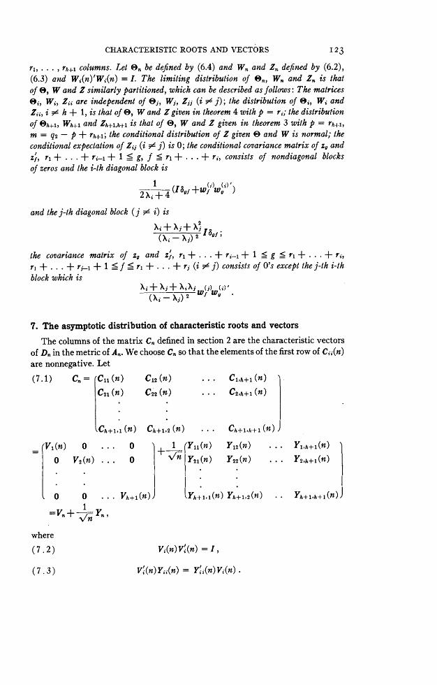
r1,... rh+4 columns. Let On be defined by (6.4) and Wn and Zn defined by (6.2),(6.3) and Wi(n)'Wi(n) = I. The limiting distribution Of On, W. and Zn is thatof 0, W and Z similarly partitioned, which can be described as follows: The matrices0i, Wi, Zii are independent of Oj, Wj, Zjj (i F6 j); the distribution of Oi, Wi andZii, i F$ h + 1, is that of 0, Wand Z given in theorem 4 with p = ri; the distributionof Oh+l, Wh+j and Zh+1,h+l is that of 0, W and Z given in theorem 3 with p = rh+j,m = q2 - p + rh+1; the conditional distribution of Z given 0 and W is normal; theconditional expectation of Zij (i F$ j) is 0; the conditional covariance matrix of z, andz1, ri + + rj_- + 1 < g, f _ r1 + . . + ri, consists of nondiagonal blocksof zeros and the i-th diagonal block is

1~~~~ (~.)'2 U+bf# +Wf Ws )

and the j-th diagonal block (j Fd i) is

Xi+ Xj+ xj bf(X1i-X)2'6

the covariance matrix of z, and z, r++ + ri_- + 1 _ g _ r1 + . . . + ri,r1 + . . . + rji- + 1 _ f _ ri + . . . + r, (i #4 j) consists of O's except the j-th i-thblock which is

(XiX+ ) 2-JW U

7. The asymptotic distribution of characteristic roots and vectors

The columns of the matrix Cn defined in section 2 are the characteristic vectorsof Dn in the metric of An. We choose Cn so that the elements of the first row of C2i(n)are nonnegative. Let

(7.1) C.= rC,,(n) C12(n) . . . C1,h+1(n)|C21 (n) C2'2 (n) . .. C2.h+l (n)

Ch+l.l (n) Ch+1,2 (n) . . . Ch+±,h+1 (n) J

_V1(n) 0 ... 0 . Y n Y12(n) .. Yl,h+l(n)O V2(n) ... 02nY (n) Y22(n) ... Y2,h+l(n)

0 0 .. Vh+Al(n) (Yh+1,1(n) Yh+1,2(n) * * Yh+l,h+l(n)J

.\n-where

(7. 2) Vi(n)V'(n) = 1,

(7.3) V$(n)Yii(n) = Yij(n)V1(n)

I24 SECOND BERKELEY SYMPOSIUM: ANDERSON

Let(7.4) tC = Xn' .

If X,. = JnCn-1, then Cn = C.J., where J,n is a diagonal matrix with diagonal ele-ments + 1 and -1. Now define V,, and Yn, in terms of Cn as V,, and Yn are in termsof Cn. First let us show that for nonrandom W,, -k W, Zn- Z (which defineXn X), f',V-* W' and Yn -Z'. We have

/ 1 '12 1 'n75n+ 4 n=(W. + V/-Z-) = (I+ W')

=K(I-77= WnZn + (W.Zn) )

= pWnZnWn+ 2WnZ)Wn

for n sufficiently large. The i-th diagonal block of (7.5) is

(7.6) Vi (n) -n)= W(n) - W.'W(n)Zii(n) W.(n) +- Tij(n)~~~~~~Wn

=W,(n) - -n Z, (n) + nTi'(n),

where the elements of Tii(n) are bounded. Multiplying each side of (7.6) on theleft by its transpose, we obtain

(7.7) I+ / [V, (n) ii(n) +Y1i(n)Vi(n)I +- Yii(n)Yii(n)

=I- wWi (n)Zi (n) + Zii (n) W,'(n) I + n- Sii (n) .n

i n~~~

Subtracting I from both sides, multiplying by Vi(n) and using (7.3) and (6.3),we find

(7.8) Yii (n) = -Vi(n) Wi(n)Zii(n) + \/n Vi(n)Ri(n).

We can show (by means of an argument similar to that used in section 4) that theelements of Vi(n)Ri(n) = Sii(n) - Vi(n)Y'j(n)Yjj(n) and of Ri(n) are bounded.Inserting (7.8) in (7.6) we obtain

(7 .9) Pi (n) = (W,, (n) - gn Zii (n) + nTij (n) ) (I+ 'Wi (n) Z'i (n)

+ nRi(n) ) W (n) + nQi(n)

for n sufficiently large. It is clear from this that Vi(n) Wiand from (7.8) thatYii(n) -Zii (as Wn - W and Zn -* Z). A nondiagonal block of (7.5) is

(7.10) -Y1ij (n) = - - W,(n)Zij(n) W,(n) + n Tij(n)

Clearly, fjj(n)-WZ-jWZj.

CHARACTERISTIC ROOTS AND VECTORS 12 5

C, and C. are different (for fixed W,, and Zn) only in that columns of one aremultiplied by -1 to obtain columns of the other. However, for n large enough thesign of the elements of the first row of eii(n) are those of Wi'(n) [= Vi(n)], whichare all positive (if the elements are different from 0). Thus CR =C, for n largeenough. Therefore, for nonrandom WK -- W and Zn -- Z, Vn - W', Yii(n) - Zi-and Yij(n) - i- WiZijWj. The discontinuities of the limiting transformation havelimiting probability 0. Thus the limiting distribution of the random matrices ORVnand Yn is the distribution of the random matrices 0, V = W', Y= -W'ZWwhere the distribution of 0, W and Z is given in theorem 5.

The distribution of 0 and V' = W has been given explicitly. From the condi-tional distribution of Z let us find that of Y. Consider first Yii, i F- h + 1

(7.11) ,ClYiiI, W) =-g{ZilI, W) w'o12 (Xi+2 i.

The covariance between two elements of Yii, say Yab and Ya'b' is

2 + 4 ( 'ba bb' + Vab'Va'b)-The matrix Yh+l,h+l is normal with mean 0 and covariance given above (for Xi = 0).Now consider Yij= - WiZ,jW,' and Yji= - WZjiWI. The joint conditional

distribution is normal with zero means. The variance of the elements in Yij is(Xi + Xj + XA)/(Xi- Xj)2 and that of the elements in Yji is (Xi + Xi + XI)/(Xi - Xj)2. The covariance between elements in Yij is 0 as are those between ele-ments in Yji. The covariance between an element Yab in Y,j and Ya'b' in Yji is

'Xi+xj+ Xi (i0G (j)(X - Xj) 2 vab' Va'b.

THEOREM 6. Letg2

D.= y[y0+ \/n rT (n) 0Hy, + \Vn rT (n)e]',,o=1

where the p-dimensional vectors yi, . .Y,y,2 (q2 > p) are independently distributedaccording to N(O, I) and rT(n) = V\ i(n- -\/X, ri + . . . + ri-1 + 1 _ g _ri + . . . + r,; Xi > Xj, i < j (i, j = r, ., h+ 1);XA+1(n) = 0. Let A. be inde-pendently distributed according to W(I, n). Define CR and 0Rn by means of (2.11),(2.12) and the conditions that cr,+. +ri- + ,,(n) > 0, ri + . . . + ri-I + 1 _g _ ri + . . . + ri (i = 1, . .. , h + 1) and 4R is diagonal with diagonal elementsin descending order. Let each of CR and 4R be partitioned into (h + 1)2 submatricesof r1, . . , rh+1 rows and r1, , rh+1 columns. Let 0e be defined by (6.4) and VRand YR be defined by (7.1), (7.2) and (7.3). The limiting distribution of 0En Vn andYR is that of 0, V and Y similarly partitioned, which can be described as follows: Thematrices 0i, Vi, Yii are independent of Oj, V,, Yjj (i $6 j); the distribution of 0i andVi is that of 0 and W given in theorem 4 with p = ri, i $ h + 1, the conditionaldistribution of Yii given Oiand Vi is normal with mean (2Xi + 4)-1Vii; the distri-bution of 0h+1, Vh+1 is that of 0 and W given in theorem 3 with p = rh+i, m =

q2 - p + rh+1; the conditional distribution of Yh+l, h+1 is normal with mean 0; the

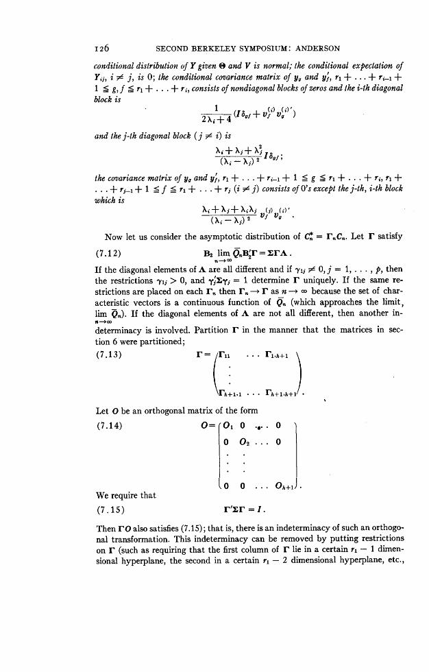
126 SECOND BERKELEY SYMPOSIUM: ANDERSON

conditional distribution of Y given 0 and V is normal; the conditional expectation ofYij, i wd j, is 0; the conditional covariance matrix of y, and y, ri + ... + ri-1 +1 _ g, f _ r, + ... + ri, consists of nondiagonal blocks of zeros and the i-th diagonalblock is

2Xj+ 4 (I uf+ Vf vg)

and the j-th diagonal block (j $ i) is

-2

-X_ j) 2Il I 822;

the covariance matrix of yg and y, ri + . . .+ri- + 1 _ g _ ri + . . . + ri, r1 ++ rj_i + 1 _ f _ ri + . . . + rj (i $ j) consists of o's except the j-th, i-th block

which is

Xi+ As+XXjVV2Now let us consider the asymptotic distribution of Cn = 7nCn. Let r satisfy

(7.12) B2 lim Q0B'r = IrA.If the diagonal elements of A are all different and if -ylji 0,] = 1,... ,p, thenthe restrictions ylj > 0, and TIZyj = 1 determine r uniquely. If the same re-strictions are placed on each r, then r r as n - because the set of char-acteristic vectors is a continuous function of QO (which approaches the limit,limrn ). If the diagonal elements of A are not all different, then another in-n-4codeterminacy is involved. Partition F in the manner that the matrices in sec-tion 6 were partitioned;(7.13) ][In ...rl,h+l

rh+ 1. . . . rh+l,h+l/

Let 0 be an orthogonal matrix of the form

(7.14) 0= 01 0 .*.. 0

0 02... 0

0 . ..0h+lJWe require that

(7. 15) rlyx I

Then rO also satisfies (7.15); that is, there is an indeterminacy of such an orthogo-nal transformation. This indeterminacy can be removed by putting restrictionson r' (such as requiring that the first column of r' lie in a certain ri - 1 dimen-sional hyperplane, the second in a certain r1 - 2 dimensional hyperplane, etc.,

CHARACTERISTIC ROOTS AND VECTORS I27

with an element in each column having a specified sign). For all n greater than someparticular integer, the same restrictions can be imposed on IF. With these restric-tions imposed, r, -4 r.

Then

(7 .16) Cn=rCn=rYn+u rYnLet

(7.17) Vn = rnVn,

(7.18) Yn = rnYnthen

(7.19) Cn=Vn+ 1

V* and Y* are functions of Vn and Yn. As n co, the functions approach limits;that is, for fixed Vn = V and Yn = Y, V* IV = V*, say, and Y-* rY = Y*,say. Thus by Rubin's theorem the limiting distribution of the random matricesV: and Yn* is that of rV = V* and rY = Y*.The distribution of V* is that of rV. The distribution of 0 is given in section 6.

The conditional distribution of Y* given V* and 0 can be found from that of Y.We have

(7.20) C I Yij I 0, v=I1' rik I{ Yki I0, v2 ) V

g {rif,hl |I,V} = 0 .

The conditional covariances are easily obtained from theorem 6. Let ya* be thea-th column of Y*. Then the conditional covariance matrix of this vector fora _ r, is

(7.21) 1 (IvW v(1)) .0r2 X+4- +Va Va ) ... 0 V

X1+ X2+2I 0

0 0 ...

= 2+-ri (I+ Va Va )r'+ E (*-,X .)2 rjri,2Xj+4where(7.22) ri= ri.

,rh+l,ij

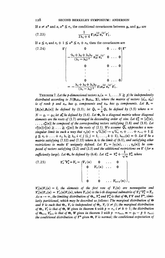
I28 SECOND BERKELEY SYMPOSIUM: ANDERSON

If a #4 a* and a, a* < ri, the conditional covariances between Ya and Ya are

1 (1) Ci)',(7.23) 2X IF F.a*Va rl

If a _ r, and r1 + 1 . a* < r, + r2, then the covariances are

(7.24) r0o 0 ... O r'

(724+ X2+ X1X2 (2) (I)'0°

0 0 0

o o ... oJXi+X2+XIX2 (2) Wi'(X-1 X2) 2 r2Va* Va rF.

THEOREM 7. Let the p-dimensional vectors Xa(a = 1, . . N _ p) be independentlydistributed according to N(Bizia + B2z2., ;), where the matrix of vectors (ziax, z'a)is of rank p and zla has qi components and Z2a has q2 components. Let Bn =

[Bi(n),B2(n)] be defined by (1.3); let Qn =-Qn be defined by (1.5) where n =

N - qi - q2; let A*n be defined by (1.6). Let On be a diagonal matrix whose diagonalelements are the roots of (1.7) arranged in descending order of size. Let Cn* = [cl(n),

cp(n)] be composed of the corresponding vectors satisfying (1.8) and (1.9). Let'r1(n)[Tr2(n) > .. .> 4,(n)] be the roots of (2.1). We assume Q approaches a non-

singular limit in such a way that rT(n) = v/Xj(n)- x/\ki, rI + . . . + ri-i + 1 <

g _ ri + ...+ ri, Xvi > Xi, i < j (i, j = 1, . . . , h + 1), 1Xh+,(n) = O. Let r be a

matrix satisfying (7.12) and (7.15) where A is the limit of (6.1), and satisfying otherrestrictions to make r uniquely defined. Let rn = [yi(n), , y,(n)] be com-posed of vectors satisfying (2.2) and (2.3) and the additional restrictions on r (for n

sufficiently large). Let 0e be defined by (6.4). Let C: = Vn*+ .Y* where

(7.2 5) rn2V: = V. = (V, (n) 0 ... 0

I 0 V2(n) ... 0

0 0 .* Vh+l(n),

V'(n)Vj(n) = I, the elements of the first row of Vi(n) are nonnegative andV (n)Yii(n) = Y1i(n)Vi(n), where Yii(n) is the i-th diagonal submatrix of rn-FYn* = Yn.As n , the limiting distribution of On, V* and Y* is that of 0, rv and Y*, simi-larly partitioned, which may be described as follows: The marginal distribution of 0and V is such that 0s, Vi is independent of 0j, V, (i 1j); the marginal distributionof Oi, V' is that of 0, W given in theorem 4 with p = ri, i # h + 1; the distributionof h+b, Vh,+j is that of 0, W given in theorem 3 with p = rh+l, m = q2 - p + rh+1;the conditional distribution of Y* given 0, V is normal; the conditional expectation of

CHARACTERISTIC ROOTS AND VECTORS I29

a submatrix YV, is given by (7.19); the conditional covariance matrix of YD and y*',r + .+ + 1 _ g,f < r + ...+ r, is

(7.26) 2X+4[riv v(i) ri +5,r1ri] + B,I+f ( + ) r,i#i

the conditional covariance between yu and yf', r, + ... + r_j + 1 . g <rl+. . .+s,rl+ . .+rj_l+1 _f _ r+ . .+rj (i j), is

Xi+xj+Xix (.j) (i)'(7.2 7) (X X+j) 2 ]priv Vg ri

where I'i is defined in (7.22) and v() is the g-th column of Vs.A special case of considerable interest is the case of ri = 1, i 0 h + 1 and

rh+l= p - . Then Yi consists of one element for i, j $ h + 1. In this caseVi = 1 for i $1 h + 1. We can easily express the conditional distribution of Ygiven Vh+l by integrating out 01, . . . , Oh. The marginal distribution of 0s isN(O, 2XM + 4Xk) and the conditional distribution of yii is N[Oi/(2Xi + 4),l/(Xi + 2)]. Oi and yii are independent of the other variables. The marginal dis-tribution then of yii is N(O, 1/2).

In this case e{ Y* I VA+l = 0. The conditional covariance between y and y',aa _ h is

h+1i

2

(7.28) aYa 2 + E j_ 2 riri

j#aThe conditional covariance between Ya* and ya**, a id a*, a, a* _ h is

(7.29) g{yayO*)Ijvh+l} = - (X. ;2aa*ura-

The conditional covariance between ya* and ya**, a _ h, h + 1 _ a* _ p, is

(7.30) a{ Yya* Vh+1} =arh+lVo*ra .

The conditional covariance between Ya and y*, h + 1 < a, a* < p, is

(7.3 1) y{* Vh*Iv ]+}=(1r a+l(I&aa*+vV* Va )rl+1 + rXj r , ai=1

Clearly, if r1 = 1, i= 1, . .. , h + 1 = p, then V,, = I, and the limiting dis-tribution of 0E and Y,* is such that the marginal distribution of Y* is normalwith mean 0 and covariances derived from above.

8. Remarks -

8.1. Use ofN and n = N - q. In section 2 we defined Q,, as - Q.. The asymptoticn

distributions obtained are exactly the same if one uses Q,, for the roots of

IB2 N Q,,B2- p2 are multiples by n/N of the roots of (2.1). These roots con-

verge also to Xi, . ., 1, respectively, and for each n the multiplicities are thei

same in the two cases. Using Q,, changes the definition of the samp'le roots again

I30 SECOND BERKELEY SYMPOSIUM: ANDERSON

by a factor of n/N. We might also define A* in terms of N instead of n and nor-malized c* in terms of N instead of n. Asymptotically the effect of using N insteadof n disappears. Rubin's theorem can be used to prove each such statement rigor-ously.

8.2. The limiting probabilities. It is interesting to see for what sequences of setsin the space of the characteristic vectors the limiting probabilities are defined. Asa simple example, suppose p = ri = 2 and : = I. We shall consider a sequenceof sets for one vector ci and another sequence for C2 defined in the same plane.Consider a segment on the unit circle in the right half plane. The regions for cl con-tain this segment and as n -X c the regions converge to the segment. The bound-aries converge as l/v/n. Consider the segment of the unit circle in the right halfplane composed of the points which are 900 from the points in the other segment.There is a corresponding sequence of regions which close down on this segment asn increases. The limiting probabilities are defined for these sequences.

8.3. Cases of special interest. Two cases of the model discussed here are of par-ticular interest. The one occurs when the "fixed variate" vectors zQ (in section 1)are composed of dummy variates; that is, variates that are 0 or 1 (see [1], for ex-ample). These can be chosen so that Bza = /Ai, a = N1 + . . . + Ni-i + 1, ....N1 + . . . + Ni (N1 + . . . + N, = N). The first N1 Xa are observations fromthe first population, etc. If we require that Ni = kiN as N -x c, then the multi-plicities of the roots of (2.1) are unchanged as N -* c.

It can be shown that if N/n[r2(n) - r2(n)] -+ 0 as n -+ c, ri + ... + ri-1 +1 < g, f _ r, + . . + ri, i 1,..., h+ 1, then 0, W., and Zn (also 0n, V*n,and Y*) can be defined in the manner of this paper and have the same limitingdistribution as given here. Thus we can weaken our conditions slightly. If Ni =kiN to within rounding error in the case mentioned above, the same theory applies.

If the fixed variate subvectors Z2a are not composed of dummy variates, in gen-eral the nonzero roots of (2.1) will be simple for all n and in the limit. Then thetheory at the end of section 7 applies.

REFERENCES

[11 T. W. ANDERSON, "Estimating linear restrictions on regression coefficients for multivariatenormal distributions," submitted to Annals of Math. Stat.

[21 T. W. ANDERSON and HERMAN RUBIN, "Estimation of the parameters of a single equation ina complete system of stochastic equations," Annals of Math. Stat., Vol. 20 (1949), pp. 46-63.

[3] R. A. FISHER, "The statistical utilization of multiple measurements," Annals of Eugenics, Vol.8 (1938), pp. 376-386.

[41 PAUL R. HALMOS, Measure Theory, D. Van Nostrand Co., New York, 1950.[51 P. L. Hsu, "On the distribution of roots of certain determinantal equations," Annals of Eu-

genics, Vol. 9 (1939), pp. 250-258.[61 , "On the problem of rank and the limiting distribution of Fisher's test function," An-

nals of Eugenics, Vol. 11 (1941), pp. 39-41.[7]--, "Canonical reduction of the general regression problem," Annals of Eugenics, Vol. 11

(1941), pp. 42-46.[81 , "On the limiting distribution of roots of a determinantal equation," Jour. London

Math. Soc., Vol. 16 (1941), pp. 183-194.[91 HERMAN RUBIN, "The topology of probability measures on a topological space," Duke Math.

Jour., to be published.