Independent investigations show that several geophysical phenomena occur on or near magnetic lines of force forming a connected region called the auroral oval and extending to a dipole latitude of 76° at noontime and 67° at midnight . "Magnetic data obtained with the Navy-APL satellit e 1963 S8G are cont ributing basic informat ion on some of the auroral oval properties. It is anticipated that these magnetic

A.]. Zmuda

data, for 1100 km altitude, will play an 1·mportant role in connecting visible auroras and their related ionosphere disturbances with phenomena occurring at altitudes considerably above 1100 km.

THE AURORAL OVAL

The aurora is one of the most impressive, beautiful, and colorful of natural phenomena.

It may have, for example, a form of a ray, drapery, arc, band, or cloud; and a color of white, violet, blue, green, or red. At certain Arctic and Antarctic locations, an aurora can be seen on practically every clear night. Occasionally an aurora appears at lower latitudes; the last one over Washington, D. C., occurred in September 1963. An aurora observed in the northern hemisphere is called Aurora Borealis or Northern Lights; in the south­ern hemisphere, Aurora Australis or Southern Lights.

Although auroral accounts date to the first century A.D. and although the aurora has been intensively studied within the framework of the contemporary science of the last century, there is yet much to be learned about the fundamentals of this intriguing subject.

Recent developments show that it is advisable to study auroral phenomena in terms of a region of the geomagnetic field which is called the auroral oval because of its oval shape and its association with the visible aurora. The Navy-APL satellite 1963 38C is yielding valuable data on the magnetic varia tions occurring on the magnetic field lines forming the auroral oval. The purpose here is to consider some of the characteristics of these resdts as well as of other geophysical phenomena relevant to the auroral oval.

2

Coordinate Systems

About 90% of the geomagnetic field of ongm internal to the earth may be represented for points above the surface, as the field of a dipole (of moment 8.03 X 102 5 gauss cm3

) located at the earth's center with its axis tilted 11.5° from the axis of rotation. The dipole axis intercepts the earth's surface at the antipodal points (geographic coordinates 78.5 ° N, 69.7° Wand 78.5° S, 110.3 ° E). A set of coordinates referenced to this dipole called dipole or geomagnetic coordinates is used. The dipole colatitude e is the angle that the radius vector to the point makes with the dipole axis; the dipole latitude A is 90° - e. The dipole longitude is measured eastwards from the meridian half-plane bounded by the dipole axis and con­taining the geographical south pole.

Figure 1 shows some station locations in a view from above the dipole pole in the northern hemi­sphere. Thule, Greenland, at a latitude of 88 ° , is near the pole. During the hours around local mid­night auroras appear over or near such well­known auroral stations as College, Alaska ; Kiruna, Sweden; and Fort Churchill, Canada-all with dipole latitudes between 64 ° and 69°. (Washing­ton, D. C., is at 51 ° Nand 350° E, geomagnetic.)

Geomagnetic local time (GLT) at a point is defined by the angle between the geomagnetic

APL Technical Digest

meridional planes through the point and the sun, respectively. Local time (L T) at a point is defined by the angle between the geographic meridional planes through the point and the sun, respectively. No distinction is made between GL T and LT in what follows, although small differences do exist and are sometimes significant.

Fig. I-Some station locations in dipole coordinates in a view from above the dipole pole in the northern hemisphere.

NOllemb er-Decelllber 1966

An Aurora

Fastie1 has recently discussed auroral observa­tions obtained with rockets. Although there are 12 basic forms of auroras, most auroras would, how­ever, have the following common characteristics: a lower border at altitude 95 to 110 km above the earth's surface, a north-south extent of order 1 km, alignment along the local geomagnetic field line, and a vertical extent of 20 to 30 km betv,reen points with one-half the peak brightness.

Light from the aurora cannot be detected in the presence of sunlight (which is of much higher intensity ), so that a visible aurora is observable only under local nighttime conditions. From the auroral stations in existence before July 1, 1957, nighttime auroras were regularly observed during the evening and early morning hours in the so­called auroral zone of latitudinal width about 10° centered at A = 67 ° . It was frequently assumed that the auroras occurred in this zone during the daytime and as a consequence the central auroral­zone angle of 67 ° was extended azimuthally around the earth. For a long time this assumption could be neither substantiated nor repudiated; the auroral stations at A = 67 ° had daylight, say, at noontime, and could not have detected an aurora even if it were there.

1 w. G. Fa~tie , " Rockets and the Aurora Borealis," APL T echnical Digest, 5, No.5 , May-June 1966, 5-10.

3

During the International Geophysical Year (IGY), from July 1, 1957, through 1958, auroral observations were regularly made at many stations set up at higher latitudes and particularly in the northern hemisphere. (The IGY was an 18-month period of an international cooperative effort to study geophysical phenomena on a global basis.) During the northern winter, with the stations in continuous darkness, visible auroras were regu­larly observed, for example, at local noontime at latitudes = 76°, and occurred simultaneously at all longitudes along the closed loop2 now being called the auroral oval. 3

Auroral Oval

Figure 2 is a downward view from above the north pole, showing the circles of dipole latitude and various time markers. The heavy line in Fig. 2 represents the projection on the earth's surface of the mean position of the auroral oval. This same line can also be interpreted as defining the inter­section with the earth's surface of the field lines marking the auroral oval. The oval has a center displaced about five degrees along the midnight meridian from the dipole pole and lies, for ex­ample, around 67 ° at midnight and 76 ° at noon. Roughly speaking, the oval is fixed with respect to the sun and the earth rotates under the oval;

SUN

r-----~----+_----+_----~--~~----~6

o

Fig. 2 --The space-time distribution of the auroral oval in dipole coordinates.

2 Va. I. Feldstein, "Some Problems Concerning the Morphology of Aurorae and Magnetic Disturbances at High Latitudes," (English translation) {;eomagnetism and Aeronomy, 3, 1963, 183-192. 3 S. I. Akasofu, " The Auroral Oval, the Auroral Substorm, and Their Relations with the Internal Structure of the Magnetosphere," Planet Space Sci ., 14, 1966, 587- 595.

4

as a consequence the posItlon of a station with respect to the oval varies with the local time for the station. For example, a station at 73 ° latitude is north of the oval at midnight; inside the oval at 0800 and 1700; and south of the oval at 1200.

When a visible aurora occurs, it appears simul­taneously at all points in the oval which also lie at or near the magnetic lines of force containing all of the following: the high-latitude boundary of the Van Allen trapping region, the maximum precipitation of energetic electrons, the polar elec­trojet, the radio aurora, and large transverse magnetic disturbances at 1100 km altitude. (Pre­cipitating particles are those which reach the lower ionosphere, say altitudes around 100 km, where they lose energy by collisions with the atmospheric constituents which are ionized and excited to emit electromagnetic radiation such as light at 3914 A, from the singly ionized nitrogen molecule.)

The polar electrojet and its magnetic field are of particular interest here. Magnetic records from high-latitude observatories show that the field ob­served at the earth's surface in and near the auroral oval has a horizontal component which is time-varying and directed southward, forming a field perturbation superimposed on the main geo­magnetic field. This auroral component is called a negative bay (or disturbance field vector or polar magnetic substorm) and is attributable to a cur­rent-the polar electroject- flowing westward at all longitudes in the ova}.4 It is presently thought that the current (a) flows principally at altitudes 100 to 120 km, (b) consists mainly of electrons flowing eastward (to produce a westward current, according to convention in electromagnetic theory), (c) has a value of about 30,000 amp, and ( d) is driven by an electric field of order 10-2

volt/ meter which is possibly directed southward, considering the anisotropic conductivity in the ionosphere. The primary auroral particles can produce ionization with secondary electrons suffi­cient for the ultimate current, but an outstanding auroral problem is to determine the mechanism which produces the driving electric field.

Primary Particles

A quantitative correlation has not yet been made between the aurora and the primary charged particles producing it, but the existing evidence points towards electrons with E < 40 ke V and principally electrons in the approximate range 1 to 10 keV. Electrons in this energy range and with

4 S. I. Akasofu, S. Chapman, and C . I. Meng, " The Polar Electro­jet." ]. Atmosph. Terr. Phys., 27, 1965, 1275-1305.

APL Technical Digest

~dequate flux have been observed in rocket flights mto auroras. See, for example, McIlwain5 and Fastie. 1

Electrons with E ~ 40 keY have frequently been observed with satellites, but these, though showing a good temporal and spatial correlation with auroras, nevertheless do not have the required total particle energy. Auroral particles are pre­cipitating particles which as earlier noted lose their energy in collisions with the atmos~heric constituents which become ionized and/ or excited to emit the auroral radiation; electrons of energy of a few ke V moving down the auroral field lines would have a height distribution of energy loss similar to the vertical profile of auroral luminosity and ionization. In many auroras hydrogen emis­sions are absent or relatively faint, which eliminate protons as the primary particles, since auroral protons would ultimately capture an electron from the auroral ionization to form excited hydrogen.

Electrons with E < 40 ke V are under intensive investigation by direct and indirect means and their role in auroral physics may soon be quantita­tively established. One approach is that of Belon, Romick, and Rees6 who infer spectra of pnmary auroral electrons from the observed vertical luminosity profile of the aurora. Some findings are: For the aurora of February 26, 1960, observed near College, Alaska, emissions from singly ionized nitrogen N~ at a wavelength of 3914 A occurred at altitudes between 82 and 285 km with the maxi­mum volume rate of 2.3 X 104 photon/ cm 3/sec at 120 km, values of one-half the peak a t 113 and 147 km, and of one-tenth, at 101 and 214 km. Integration under this luminosity profile, corre­sponding to an observation from directly under the aurora, yields an in tensi ty of 1.14 X 1 05 R ayleigh or 1.14 X 1011 photon/ cm2/ (column) sec, an in­tensity which places this aurora in the class of International Brightness Coefficient (IBC ) 3, and which is about one-tenth of the illumination at the earth's surface from the full moon. (The R ayleigh is the photometric unit used in auroral studies' it is an emi~sion rate of ( 106/4-7r)photon/ster/sec/~m2.) Electrons of energy 1 ke V to 30 ke V produced the major portion of the auroral light and ionization. The total particle flux was 5.8 X 1010 electron/ cm 2

sec; the total energy flux 380 erg/ cmj!sec.

5 C. E. McIlwain , " Direct Measurements of Protons and Electrons in Visible Aurorae ," 1st Space R es. Proc. Int ern . Space Sci . Symp ., Nice 1960, (ed. H. Kallmann-Bijl ), North Holland Publishing Co., Amsterdam, 1960, 715-720.

6 A. E. Belon, G. J. Romick, and M. H. Rees, "The Energy Spec­trum of Primary Auroral Electrons Determined from Auroral Luminosity Profiles ," Plane t Space Sci., 14, 1966, 597-615.

Novembe1'-Decem ber 1966

It is worth emphasizing that the above quanti­ties relate to a relatively bright aurora, IBC-3. Belon, Romick, and Rees studied a total of 16 auroral arcs, with the total associated electron flux ranging between 2.9 X 109 and 1.1 X 1011

electron/ cm2 /sec and the total energy, between 28 and 590 erg/ cm2/sec. The average energy flux of electrons > 1 ke V precipitated into the auroral zone is 3 to 5 erg/ cm2/sec. 7

Power

The aurora of February 26, 1960, had a north­south width of 6 km and probably extended azimuthally along the entire oval, of length 1.23 X 104 km. The total power required to sustain the auroral oval present at this time then becomes 2.8 X 1017 erg/ sec or 2.8 X 1010 watt, a value 11 % of that for the total electrical power presently being generated by utilities in the United States, 2.5 X 1011 watt.

One potential source of auroral power is the solar wind, an electrically neutral stream of elec­trons and protons continuously ejected from the sun. The proton velocity averages 5 X 107 cm/ sec and the proton number density near the earth is 5 particles/ cm3, yielding an energy flux of 0.5 erg/ cm2/ sec in the solar wind. s The total geomagnetic field presents to the solar wind a circular f ron tal area of radius about 12 earth radii ,9 so that the power input from the solar wind equals ~.3 X 1012

watt, about 300 times larger than that required to sustain an aurora of IBC-3.

From power considerations alone, the solar wind could be the source for any aurora but its role if any, is not yet established. The av~rage energy' of the solar-wind proton is 1. 3 ke V; and from argu­ments based on electrical neutrality for the wind, it is expected that the electrop and proton veloci­ties a re equal, in which case the average electron energy is 0.7 e V, much less than the ke V energies of auroral electrons. (To penetrate through the atmosphere above the aurora and to produce an aurora at the altitudes where they regularly ap­pear, ~ 100 km, primary electrons must have an energy of at least a few keV.) If the solar wind supplies the auroral power, then an outstand­ing unsolved problem is that of determining the

7 B. J . O ' Brien and H. Taylor, " High L atitude Geophysical Studies with Sa tellite Injun 3, Part 4. Auroras and their Excitation " j. Geophys. R es., 69, 1964, 45-63. '

8 M. Neugebauer and C . W . Snyder, " Mariner 2 Observations of the Solar Wind , Part 1. Average Properties," j. Geophys. R es. 71 1966, 4469- 4484. ' ,

9 J. A. Van Allen , " Some General Aspects of Geomagnetically Trapped R adiation ," Radiation Trapped in the Earth's Magnetic Field (ed . B. M . McCormac) , D . Reidel Publishing Co. , Dordrecht­Holland, 1966, 65- 75.

5

means of energy transfer from the solar wind to the aurora or relatedly of finding the auroral ac­celeration mechanism and the process by which solar wind particles attach to auroral field lines. Contrary to the initial expectation, trapped par­ticles in the Van Allen zone do not contribute III

a fundamental manner to auroral phenomena.

Magnetic Field Configuration and Trapping Region

Figure 3 shows the geomagnetic lines of force in the noon-midnight meridional plane from a modepo,l1 consisting of the following field sources:

Fig. 3~Magnetic field lines in the moon-midnight meridian resulting from the interaction between the solar wind and the field of the geomagnetic dipole.

the geomagnetic dipole; currents in the magneto­pause (or boundary of the geomagnetic field) with a geocentric distance of 10 earth radii (64,000 km) at the subsolar point; and currents in the neutral sheet region, on the nightside and be­ginning at about 10 earth radii. The geomagnetic field vanishes in the neutral sheet region which separates an antisolar-directed field in the southern hemisphere from the solar-directed field in the northern hemisphere.l~ The magnetopause and

10 D . ] . Williams and G. D. Mead, "Nightside Magnetosphere Con­figuration as Obtained from Trapped Electrons at 1100 km," J. Geophys. Res., 70, 1965, 3017- 3029.

11 G. D . Mead , " The Motion of Trapped Particles in a Distorted Field," Radiation Trapped in the Earth's Magnetic Field (ed. B. M . McCormac ), D . Reidel Publishing Co. , Dordrecht-Holland, 1966, 481-490. .

12 N. F . Ness, " The Earth's Magnetic Tail," J. Geophys. R es., 70, 1965, 2989-3005.

6

neutral-sheet currents result from the interaction between the geomagnetic field and the plasma constituting the solar wind, an interaction produc­ing a compression of the field on the dayside and an extension, or drawing out, on the nightside. An elongated cavity forms in the plasma by the turning aside and back of the positively and nega­tively charged plasma particles. The geomagnetic field is confined inside this cavity, now called the magnetosphere, whose existence was predicted by Chapman and Ferraro/3 in their studies on mag­netic storms.

The number on a field line in the illustration refers to the geomagnetic latitude where the line intercepts the earth's surface. Field lines with sur­face latitudes < 60 ° are unaffected by the rela­tively weak fields of the magnetopause and neutral sheet currents and represent the lines of force of the geomagnetic dipole. The 60 ° line on the day­side is the only dipole-like line shown in this illustration. The higher-latitude lines, however, depart considerably from a dipole-like configura­tion and reflect the compression and expansion earlier noted as well as the following characteris­tics. There exists a critical latitude which separates the closed from the open field lines. A closed field line is one such as the 75 ° line on the dayside which intercepts the earth's surface in both hemi­spheres and crosses the equator; an open field line, for example, either of the 85 ° lines, stretches out into the magnetosphere tail.

Stable trapping of charged particles occurs only on closed field lines, since these particles bounce back and forth between their mirror points, one in each hemisphere, while drifting azimuthally around the world. Th~ white region in Fig. 3 represents the region of stable trapping, or Van Allen zone. On the midnight side the trapping region extends to about the 67 ° line, whose sur­face latitude is comparable to the critical latitude and that of the auroral oval for this time. At noontime the trapping-region boundary and the auroral oval have a surface latitude around 76° which is considerably less than the value of the noontime critical latitude in this model, which has been calculated to lie between 80 ° and 85°. The source of this difference is presently unknown, but may lie in a mechanism which at high alti­tudes so distorts the 76 ° noontime field line that this field line connects to the solar wind whose particles will then find ready entry into the lower ionosphere.

The field lines forming for all longitudes the high-latitude limit of the stable trapping region

13 S. Chapman and V. C. A. Ferraro, "A New Theory of Magnetic Storms," Terr . Magn., 36, 1931, 77-79, 171-186.

APL Technical Digest

intercept a region that lies either along or near the auroral oval.

Magnetic Disturbances at 1100 km in the Auroral Oval

The author, in collaboration with J. H. Martin and F. T. Heuring, is engaged in studies of mag­netic variations occurring at a satellite altitude of 1100 km and on field lines in or near the auroral oval. 14. 1 5

Satellite 1963 38C (or 5E-1 in APL nomencla­ture) was launched on September 28, 1963, into a nearly circular polar orbit at altitude 1100 km; it contains an array of particle detectors, a mutually orthogonal set of three Schonstedt flux­gate magnetometers, and a permanent bar magnet of moment 7 X 104 gauss cmS used for magnetic stabilization. The satellite tends to align its bar axis along the local field direction as would a compass having three degrees of freedom and sub· ject to geomagnetic torques. The angle between the bar axis and the geomagnetic field is typically less than 6 0; for the region here considered the natural period of the satellite is about 7.7 minutes.

The magnetic data are for variations in a direc­tion transverse to the stabilizing bar magnet and, hence, practically transverse to the local geomag­netic field. The data were obtained as the satellite traversed a north-south arc of about 50° near a command ground station either at the Applied Physics Laboratory or at Anchorage, Alaska.

Figure 4 shows the sample output from the magnetometer with commutator lock on this chan­nel, with a - 1390y calibrate field (1 y = 10-5

gauss), and with some labels added to facilitate discussion. One-second time markers appear in the upper part of the illustration. During the period tl to t2, 0.314 second, the output represents the resultant of an axially directed calibration field of -1390y and the component of the ambient field along the fluxgate axis. At time t~ the calibration field is removed and the magnetometer measures the ambient component alone until ta (with ts - t~

also equalling 0.314 second), when the calibration field is again applied and the two-step cycle re­peated. With the aid of the telemetry reference voltages, these data yield continuous values for the ambient field component along the magnetometer axis. The field values have a regular and relatively slow change resulting from the rotational motion

14 A. J. Zmuda, J. H. Martin, and F . T. Heuring, "Transverse Magnetic Disturbances at 1100 km in the Auroral Region," J. Geo­phys. Res., 71, 1966, 5033- 5046. ]5 A. J. Zmuda, F. T. Heuring, and J. H. Martin, "Dayside Mag­netic Disturbances at 1100 km in the Auroral Oval," to be published in J. Geophys. Res., 1967.

November-December 1966

of the satellite as it tends to align itself along the local geomagnet;c field. In this case the compo­nent decreases linearly with time and the total change is 70y for the 19-second interval shown in the illustration.

1826:07 UT MARCH 10. 1964

1826:20 UT

.. '-7" -""""" , -.. '\ . ,. -., ,,.,..,... 11:._---- ,.. ,... ,. . . , t, tz

Fig. 4-Sample of raw data from X magnetometer with commutator locked on this channel and with a calibration field of '-1390y. These field values have a regular and relatively slow change resulting from the rotational motion of the satellite as it tends to align itself along the geomagnetic field.

~~~~~~.~~ .. -~.~-~ .. ". ... ,.. ... ",,..,.-,.-

Fig. 5-A transverse magnetic disturbance in the period 1826:29 to 1826:41 UT on March 10, 1964, as the satellite crossed field lines forming the auroral oval.

Figure 5 shows the magnetometer data for the period immediately following that in Fig. 4. At 1826: 29 UT the values start to increase and de­viate from the trend present in t < 1826: 29 UT. The departure is marked and readily recognizable and persists until about 1826:41 UT, at which time normal values begin to appear-normal in the sense that the field values at and slightly be­yond t = 1826: 41 UT are the expected extra pola­tions of the values existing in the predisturbance period t < 1826: 29 UT. The transverse magnetic disturbance occurred in the period 1826: 29 UT ~ t ~ 1826: 41 UT and considering the orbit data, occurred as the satellite crossed the field lines in part of the auroral oval.

Except for a relatively small and readily remov-

7

able effect caused by the satellite rotation in the geomagnetic field, the field variations in Fig. 5 represent the transverse field changes found as the satellite crosses at 1100 km altitude the field lines of the auroral oval. The variations regularly oc­cur- out of 246 data passes into the auroral-oval region, transverse magnetic disturbances were de­tected on 210 (85%).

Figure 6 shows the temporal variation of the oval boundaries for magnetic quiet conditions dis­cussed in terms of the dipole latitudes where the auroral oval field lines intersect the earth's surface. The southern boundary As lies around 67 ° at 2300-0100 LT and increases to 73° at 0600-0900 L T, and then rises to between 76 ° and 77 ° be­tween 1100 and 1700 LT. Within the oval, several, say two to six, distinct quasi-sinusoidal magnetic variations characteristically exist. These variations are often separated by narrow regions without variations and often contain one principal dis­turbance. Further description of the temporal and / or spatial dependence present during the in­dividual passes is not presented, but the position of the northern boundary An is shown. This boundary lies at 70 ° around local midnight and rises to about 80° for the entire period 1200-1800 LT. Both boundaries move southward as magnetic activity increases. Magnetic disturbances are ab­sent between (a) A = 35°, the minimum lati­tude observed, and the southern boundary of the oval, and (b) the northern boundary and A = 85 °, the highest latitude sampled.

8 1 r----r---.------.------.-~~

o 00 00

o

69~~=0--~----~------~----~----~

o

65L-___ -L ___ L-_ __ -L _____ ~ ____ ~

22 02 06 W LOCAL TIt0~ (hours)

Fig. 6--The temporal variation during magnetic quiet conditions of the southern (As) and northern (An) boundaries of the auroral oval.

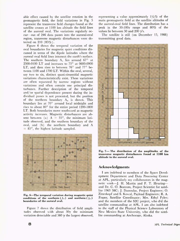
Figure 7 shows the distribution of field ampli­tudes observed with about 30y the minimum variation detectable and 560 y the largest observed,

8

representing a value approximately 11'2 % of the main geomagnetic field at the satellite altitudes of the auroral-oval field lines. The distribution has a peak in the 50-100y range and 80% of the values lie between 50 and 200 y's.

The satellite is still (on December 15, 1966) transmitting good data.

Fig. 7-- The distribution of the amplitudes of the transverse magnetic disturbances found at 1100 km altitude in the auroral oval.

Acknowledgments

I am indebted to members of the Space Devel­opment Department and Data Processing Center at APL, particularly m y collaborators in the mag­netic work- J. H. Martin and F. T. Heuring­and Dr. C. O . Bostrom, Project Scientist for satel­lite 1963 38C; .J. Dassoulas, Project Engineer; O. Zitterkopf and S. Kov"al, Payload Engineers; R. A. Frazer, Satellite Coordinator ; Mrs. Ethyl Fyler; and the members of the S2C project, who did the satellite commanding at APL. I am also indebted to the staff of the Physical Science Laboratory of New Mexico State University, who did the satel­lite commanding at Anchorage, Alaska.

.\PL TecJl7licai Digest