The Australian Real-Time Fiscal Database: An Overview and

an Illustration of its Use in Analysing Planned and Realised

Fiscal Policies∗

by

Kevin Lee†, James Morley††, Kalvinder Shields††† and Madeleine Sui-Lay Tan

Abstract

This paper describes a fiscal database for Australia including measures of government

spending, revenue, deficits, debt and various sub-aggregates as initially published and

subsequently revised. The data vintages are collated from various sources and provide

a comprehensive description of the Australian fiscal environment as experienced in real-

time. Methods are described which exploit the richness of the real-time datasets and they

are illustrated through an analysis of the extent to which stated fiscal plans are realised in

practice and through the estimation of fiscal multipliers which draw a distinction between

policy responses and policy initiatives. We find predictable differences between plans and

actual fiscal policy, consistent with a desire of the government to appear more prudent

than in reality, and a larger multiplier for policy initiatives than implementation errors.

Keywords: Real-time, Australian Database, Revisions, Fiscal Policy, Government Spend-

ing, Government Revenues

JEL Classification: C32, D84, E32

∗†University of Nottingham, UK; ††University of Sydney, Australia, †††University of Melbourne, Aus-

tralia. Version dated October 2018. Financial support from the ARC (Discovery Grant DP140103029) is

gratefully acknowledged. Corresponding author: Kalvinder Shields, Department of Economics, University

of Melbourne, Victoria 3010, Australia (k.shields@unimelb.edu.au).

[1]

1 Introduction

It is now widely recognised that empirical policy analysis can be seriously misleading if it

is conducted using the most recent vintage of available data as opposed to the data that

was available at the time decisions were actually made. Revisions in data mean that the

measurements of historical outcomes published today may differ substantially from the

data on which plans were made and so ‘real-time’ datasets, containing all the vintages

of data that were available in the past, are required to fully understand the plans. A

substantial literature has now grown, developing the methods required for the analysis of

real-time datasets and their use in prescribing and evaluating policy.1 However, whilst

there have been many studies of the use of real time data in monetary policy reaction

functions, there have only been a handful of studies in the area of fiscal policy: there are

no papers on fiscal policy in the extensive survey by Croushore (2011) on papers using

real time datasets, for example. This has become an important omission as the recent

global economic downturn and increasing levels of public debt have directed attention

towards the dynamic responsiveness of fiscal policy over the economic cycle. This has

raised questions, inter alia, on how planned policy adjusts in the face of business cycle

conditions, the ways in which expenditure plans are constrained by solvency and other

long-horizon considerations, and the ways in which actual expenditure relates to planned

expenditure at different points in the business cycle.

One reason why fiscal policy analysis is typically undertaken using only ex post data is

due to the lack of datasets that include and maintain a comprehensive set of fiscal variables

over a reasonable time span and frequency appropriate for time series analysis. The real

time ‘ALFRED’ database at the Federal Reserve Bank of St Louis contains the most

comprehensive set of fiscal variables with a reasonable time dimension and frequency but,

of course, covers the US only. The Reserve Bank of Philadelphia’s real time database, the

OECD’s real time database, the ECB-EABCN’s EU area-wide real time database, and

the recently available Australian Real Time Macroeconomic Database all include some

1See, for example, Croushore and Stark (2001) and Croushore and Evans (2006), the October 2009

special issue of the Journal of Business and Economic Statistics and the literature on monetary policy

decisions (e.g. Orphanides and van Norden, 2002, and Garratt et. al. 2009, among others).

[1]

fiscal variables although not in as much detail as that available in ALFRED.2 For this

reason, most empirical studies attempting to look at fiscal policy using real time data have

focused on the use of real time measures of output only (see Forni and Momigliano, 2005,

for instance) but important results for policy are found in those cases where real-time fiscal

datasets are used. For example, important insights have been obtained in assessing the

pro- or counter-cyclicality of discretionary fiscal policy on the basis of studies which have

constructed their own real-time databases for select fiscal indicators; see, for example,

Golinelli and Momigliano (2006), Bernouth et al. (2008), Holm-Hadulla et al. (2012),

and Cimadomo (2012).3

The ready availability of a real-time fiscal dataset is potentially very useful therefore

and this paper describes how we constructed such a database for Australia. The vin-

tages of data are collated from various sources and accommodate multiple definitional

changes, providing a comprehensive description of the fiscal environment as experienced

by Australian policy-makers at the time decisions are made. The database is available

through the University of Melbourne along with a Data Manual describing the sources

and definitions of the series in more detail than is possible in this paper; see Lee, Morley,

Shields and Tan (2015). The description of the database provided in Section 2 below

gives an overview of the structure and content of the database and illustrates some of the

difficulties in drawing inferences on fiscal policy on the basis of data that is subject to

revision. Section 3 focuses on the gap between planned and realised policies as measured

in real time and their use in measuring the fiscal multiplier, providing an illustration of

the insights provided by the data and its implications for understanding the role of fiscal

policy in the macroeconomy. Section 4 offers some concluding comments.

2The named databases

are available at http://alfred.stlouisfed.org, http://www.philadelphiafed.org/research-and-data/real-

time-centre/realtime-data, http://stats.oecd.org/mei/, http://www.eabcn.org/data/rtdb/index.htm and

http://www.economics.unimelb.edu.au/RTAustralianMacroDatabase, respectively.3To give a sense of what this data collection involves, we note that Golinelli and Momigliano (2006)

compile a real-time database for government primary balance from the OECD’s bi-annual Economic

Outlook; Holm-Hadulla et al. (2012) construct a real-time database of government expenditure for the

EU economies from annual updates of the EU’s Stability and Convergence programmes; and so on.

[2]

2 An Overview of the Australian Real-Time Fiscal Database

2.1 Structure and Content

The Australian Real-Time Fiscal Database includes a total of twelve variables relating to

budget outcomes over time plus nine variables describing the evolving state of the gov-

ernment’s debt/wealth. The data is collected primarily from the annual Commonwealth

Budget which consists of several documents known as Budget Papers, and real-time fiscal

data is mainly found in Budget Paper No. 1. The data vintages each match the corre-

sponding budget publication and are available on an annual basis therefore. The time

span of the variables in the data varies, running from Australian Federation in 1901 to

the present day for some variables while others are much shorter (e.g. those variables

defined following a change in the accounting system in 1998 are only available from the

1999 vintage onwards). The specifics of data availability for each series are provided in

Table A1 of the Appendix. Detailed information on the series are provided in the Data

Manual.

The variables relating to budget outcomes are set out below:

Table 1: Summary of Budget Data

Outlays Revenues

Spending on Goods and Services⎛⎜⎜⎜⎜⎜⎝of whichHealth

Education

Defence

⎞⎟⎟⎟⎟⎟⎠

⎛⎜⎜⎜⎜⎜⎝

⎞⎟⎟⎟⎟⎟⎠

Income Tax

(or Direct Taxation)

Expenditure Tax∗

(or Indirect Taxation)

Spending on Capital Goods Other Revenue

Transfers⎛⎜⎝of which Welfare

Pensions

⎞⎟⎠ ⎛⎜⎝

⎞⎟⎠Debt Interest Paid

Total Outlays

= + + +

Total Revenues

= + +

[3]

The evolution of these series over 1947-2014 is described in Figure 1a - 1d. Figure

1a shows the time series of , , and measured in nominal terms and as first

published after one year (i.e. +1 , for example, showing the first-release of the realised

observations). Figure 1b shows the same series but expressed relative to (first-release)

nominal GDP. Figures 1c - 1d show the time series of , and expressed in nom-

inal terms and relative to GDP respectively, again based on first-release data.4 On the

expenditure side, the plots show the total $ outlay rising rapidly, but relatively smoothly,

after the inflationary period of the seventies. The components (transfers, expenditure

on goods and services, and capital spend) also rise reasonably smoothly, although there

are genuine shifts in this composition over time and also evidence of breaks due to mea-

surement conventions following the move to an accruals accounting system in 1998-99

as discussed below. Perhaps surprisingly, the plots of Figure 1b show a high degree of

constancy in the expenditures relative to output over the period, with the ‘Great Ratio’

of total outlay to output taking an average value of 26% and lying in the range 24-28%

for most of the sample. There is a little more variability in the component parts, but

these are reasonably constant too, suggesting the presence of strong political and social

pressures to maintain and control the size of government relative to the economy as a

whole. On the revenue side, Figure 1c illustrates that Income (or Direct) Taxation makes

up the largest portion of Total Receipts, contributing around two-thirds of the total tax

take over the sample and with this contribution rising a little over time. Figure 1d again

shows the striking constancy of total outlays when expressed relative to total output, sug-

gesting further political and social equilibrating pressures to maintain a broadly balanced

budget.

The database also includes series describing the evolving debt/wealth position of the

Federal Government. These include:

• Debt, measured in three alternative ways: Net Debt, ; Gross Debt, ; Public

Debt, ;

4Note that expenditure taxes¡

¢are raised through taxes such as GST and excise duties. This

is not to be confused with tax expenditures which refer to the revenue foregone from concessions and

exemptions.

[4]

• Interest payments, measured in three alternative ways: Net Interest Outlays ;

Commonwealth Interest Liability ; and Total Interest Liabilities,

; and

• Wealth, again measured by three complementary variables: Net Worth ; Net

Operating Balance ; and Net Financial Worth

.

The existence of the various different measures of similar concepts reflects the complexity

of government accounting standards and practices. For the debt series, ‘gross debt’ and

‘public debt’ both refer to the stock of debt held by the government but the former refers

to debt held by both Commonwealth and State governments while the latter measures

the stock of debt held by the Commonwealth government only. ‘Net debt’ differs from

these two measures in that it is a flow variable and indicates the net position of debt held

by the Commonwealth general government. It is a measure that is used as a standard

to compare debt positions across different countries. The interest payment variables are

similarly related: ‘commonwealth interest liability’ refers to the interest owing on the

stock of public debt whereas ‘total interest liability’ refers to the interest due on the stock

of debt held by both the Commonwealth and States. The ‘net worth’ and ‘net financial

worth’ variables reflect the wealth position of the Commonwealth government, the latter

focusing on that part of net worth held in the form of financial assets and liabilities.

‘Net operating balance’ refers to the viability of the government position, showing the

difference between total revenue and total expenditure in the operating statement. More

complete details on the coverage of the data is provided in Table A1 of the Appendix and

in the Database Manual.

We also provide data on three important constructed variables:

• The Public Sector Financial Surplus (or ‘Cash Balance’), = −, which shows

the excess of receipts over total outlays on all its activities;

• The Primary Surplus = − ( − ) showing the financial surplus of the

government’s revenues over its spending but abstracting from interest payments on

debt; and

[5]

• The Stock-Flow Residual = − (−1 − ) which aims to reconcile the budget

balance sheet outcomes with the evolving debt position.

The first two of these are the focus of much policy discussion reflecting the govern-

ment’s spending decisions relative to its ability to finance these within the year. The

stock-flow residual is equally important in understanding government’s financial con-

straints over the longer term. Specifically, we note that, if changes in liabilities are

the result of “above-the-line” budgetary operations only, then debt in would equal

(1 + )−1 + = −1 + . In practice, however, debt liabilities are influenced

by a whole range of additional factors, including privatisation proceeds, off-budget oper-

ations, gains and losses on (below-the-line) financial operations; valuation changes due to

exchange rate movements and central bank deficit financing, such as purchases of govern-

ment debt (seigniorage). These values can be very large at times and can therefore, have

a considerable impact on government’s plans over the longer term.

The variables in the database are presented in a common format. There is an Excel

workbook for each of the variables containing a summary of the details of the data (source,

definition, etc.) on the first sheet and the raw data in a second sheet. If we denote a

variable at time − by − and the measure of this magnitude as published in time

by − , then the time- vintage of data typically includes the observations 1, 2,...,

. The observation shows the value of the variable that the government plans to

spend in year as published in year . The observation −1 shows the first-release of

the measure of −1, taking into account that there is usually a one year delay in the

release of data, and the observations − = 2 shows the time measures of past

values accommodating any revisions. The raw data presented in the second sheet is in

the form of “data triangles” where each column of data relates to a data vintage so that

the successive columns grow longer each period to give a triangular shape to the dataset.

The rows show the published measure for the same observation at different vintages so

the revisions to a particular observation can be tracked by looking horizontally across the

spreadsheet.

[6]

2.2 Unrealised Plans, Definitional Changes and Revisions in Australian Fis-

cal Data

The various vintages of data show how the measurement of a variable might change

over time. These are often best expressed in proportional terms and, in what follows,

we use upper case letters to denote the value of a variable and lower case to denote its

logarithm; i.e. = log(). Our real time dataset includes measures of the planned

values of variables (e.g. ) as well as the subsequent measures of the actual value of

the variable (+, = 1 2 ). Comparison with the first-release data +1 shows the

extent to which the stated plans were or were not realised, but changes in the measures

of the actual outcomes can also occur, either through ‘revisions’, based on the arrival of

new information on the series, or through a change in the way a concept is conceived; i.e.

involving a ‘definitional change’.

Definitional changes produce once-and-for-all shifts in a series, they typically occur

only periodically and their timing and nature are well-documented. This means that

their effect can usually be readily taken into account by a simple scaling of the pre-change

data by some additive or multiplicative factor. Fiscal data is particularly vulnerable to

definitional changes because public spending can have multiple purposes (for example,

spending on health or education involves an element of investment as well as immediate

consumption). Further definitional changes can arise because the role and scope of the

State changes over time, because responsibility can switch across different agencies (State

versus Commonwealth for example), and because there is often a political dimension to

fiscal decisions. Definitional changes that have had particularly wide-ranging impacts on

fiscal data include:

• The 1910 and 1966 currency changes: from the British pound to the Australian

pound in 1910, and to the Australian dollar in 1966;

• The 1974 accounting framework change: when the 1974-75 Budget switched froman accounting classification to a functional classification, aligning expenditures with

function rather than portfolios due to an appropriations system within the legal

framework, as previously;

[7]

• The 1994 accounting year change: when the Budget release day was moved fromthe first quarter of the fiscal year to mid-May;

• The 1996/97 definitional changes: when net advances are excluded from the reportedmeasure of outlays;

• The 1998/99 legal reform: the Charter of Budget Honesty Act 1998 introduceda mid-year update to the budget, a move from a cash accounting to an accrual

accounting system and, in 1999, the reporting of new accrual Government Financial

Statistics (GFS) variables in the budget5; and

• The 2008 reporting standards reform: the introduction of a new accounting sys-

tem (AASB 1049) harmonised the ABS GFS and AAS 31 reporting standards used

previously. Major differences between these systems relate to accounting for as-

set write-downs (treated as operating expenses under AAS 31 but negative equity

revaluations pursuant to the GFS framework), other gains and losses on assets (not

included as revenues or expenses under GFS), bad and doubtful debts (not recog-

nised under the GFS framework) and the acquisition of defence weapons platforms

(capitalised and depreciated under AAS 31 but expensed at the time of acquisi-

tion pursuant to the GFS framework)6. Where the GFS differs from accounting

standards, a reconciliation and explanation is required under the new AASB 1049

system.

It is well understood that definitional changes of this sort will effect measurement. But

data “revisions” can also be substantial because, for example, revenue collection, auditing

of accounts and collating information on spending across government departments are

all time consuming processes. Published data often supplements raw source data with

5The differences between cash versus accrual accounting terms are noted. However, for comparability

across time and for ease of narrative, cash and accrual terminologies are used interchangeably. For

example, outlays with expenses/expenditures, and receipts with revenues, wherein the cash balance is

defined as the simple difference between receipts/revenues and outlays/expenditures.6See full explanation at ABS or summary of differences here:

http://dro.deakin.edu.au/eserv/DU:30077129/wines-australiangovernment-post-2015.pdf

[8]

‘modelled’ data that anticipates the arrival of additional and/or more reliable data and

so revisions in measures of realised fiscal magnitudes can continue for some time.

Figures 2a and 2b illustrate some of the effects of data definitions and revisions in the

Australian fiscal data. Figure 2a shows the measure of the surplus in 1948/49 as reported

first in 1949/50 and then subsequently in publications dated through to 2015/16; i.e.

194849, = 194950... 201516.

7 The measure refers to the surplus in a given year but

it experiences a number of clear and distinct changes, sometimes more than fifty years

later, to reflect the definitional changes flagged above. Indeed, while it is not easy to see

from this Figure, the measure of the 1948/49 surplus switches from negative to positive in

1996, highlighting the insights that can be lost in working only with final-vintage datasets.

The Figure also shows measures of the primary balance in five later years - in 1958/59,

1968/69, 1978/79, 1988/89 and 1998/99 - again as first-released and then in subsequent

publications. These measures also undergo considerable shifts to reflect the definitional

changes mentioned above. Of course, the plots also capture the (more modest) effects of

data revisions which typically show as adjustments in the measures over a small number

of years after the first-release.8

The measures in Figure 2a are in nominal terms and so the size of the surpluses, and

definitional changes involved, are larger at later dates (and particularly after the seventies)

simply reflecting rising prices. Figure 2b considers the real surpluses therefore, expressing

the series as a ratio to the first-release measures of nominal output. The break points

associated with definitional changes are, of course still apparent and, in comparison with

Figure 2a, there is additional time-variation in the series introduced through updates on

the output data. It is interesting to see that, having scaled by output level, the sizes of

the definitional shifts now appear larger for earlier dates than for later ones, suggesting

that it is less disruptive to update observations from the near past than the distant

past when definitional changes are introduced. These measurement issues potentially

introduce systematic features into the data therefore which are difficult to overcome but

7The 1948/49 statistic was not reported in the 1962/63, 1963/64 or 1964/65 publications and so the

statistics plotted for these dates are assumed unchanged from those published in 1961/62.8As it turns out, revisions in the primary balance statistics are driven primarily by revisions in data

on receipts, with government spending figures relatively stable after first release.

[9]

which cannot be ignored in empirical work. One approach to the problem is to conduct

the analysis on transformed data (e.g. working with differences or even differences in

differences), but our recommendation is to deal with the effects of definitional changes

on a case-by-case basis prior to any analysis. This has the advantage that adjustments

to the data can take into account any known information relevant to the change while

leaving the interpretation of the series and any relationships between series unaltered.9

3 Using the Real-Time Fiscal Data: Fiscal Plans and Outcomes

The importance of the use of real-time data is best conveyed by looking at a specific issue

and in this section we make use of the real-time budget data to examine (i) whether the

government’s fiscal plans are realised and, to the extent that they are not, whether there

are any systematic patterns in the gap between plans and outcomes; and (ii) whether the

information on plans and outcomes provides insights on the usefulness of fiscal policy in

demand management.

These are important questions. If the government announces in year that it plans to

spend but it turns out that spending is +1 6= and that this gap is systematically

related to information that was known at , then the government is either deceitful or inept.

The same applies for government announcements and realisations of revenues, and for

measures of the overall financial surplus, , although the nature of the deceit/ineptitude

differs between these. A finding that government spending and overall spending turns out

to be systematically higher than announced, say, means the government is simply spending

beyond its stated intentions; if spending is systematically higher than announced but the

overall deficit turns out as planned, the government has expanded the size of government

beyond its announcements but is balancing the books as it does so.

The second question relates to the size of the fiscal multiplier. This has attracted con-

siderable attention over recent years as many governments have turned to fiscal policies

following the global financial crisis and given the constraints imposed on monetary policy

by the zero lower bound on interest rates. Several recent studies have employed VAR

9See the discussion in Garratt et al (2008) and Clements and Galvao (2013) on the pros and cons of

using levels or differences in real-time measures of output when estimating the output gap.

[10]

models to isolate government spending shocks and to trace out their dynamic effects on

output to estimate the size of the multiplier10. However, these rely on potentially contro-

versial identifying assumptions and are undermined by the ‘fiscal foresight’ problem. This

problem arises because it is difficult to quantify the output effects of agents’ reactions to

spending plans that have been announced but not yet implemented if the investigator uses

output and spending data alone. Lee, Morley, Ong and Shields (2018) [LMOS] address

these difficulties in a VAR analysis of the US multiplier using data on spending plans

alongside data on actual spending. This work finds that the multiplier effect of spending

undertaken in reaction to adverse circumstances (‘policy responses’) is approximately half

the size of the multiplier effect of planned spending (‘policy initiatives’). This idea has

important implications for macroeconomic policy and can only be examined empirically

employing real-time fiscal data of the sort we have collated here for Australia.

3.1 The Modelling Framework

Both of the questions raised can be examined through a time series analysis of the differ-

ent measures of spending and receipts that are available in our database. For example,

focusing on the spending data first, an analysis of the interplay between spending plans

and outcomes can be conducted in a simple VAR framework, as exemplified by:

G =

⎛⎜⎜⎜⎜⎜⎝−2 − −1−2

−1 − −1−1

− −1

⎞⎟⎟⎟⎟⎟⎠ = A0 +A1

⎛⎜⎜⎜⎜⎜⎝−1−3 − −2−3

−1−2 − −2−2

−1−1 − −1−2

⎞⎟⎟⎟⎟⎟⎠ +

⎛⎜⎜⎜⎜⎜⎝1

2

3

⎞⎟⎟⎟⎟⎟⎠ (3.1)

= A0 +A1G−1 + ε

Here, −2− −1−2 shows the revision in the measures of spending in time −2 as revealedbetween the publications in −1 and . The coefficients in the first rows of the 3×1 vectorA0 and the 3×3 parameter matrix A1 will be non-zero if there are systematic elements in

these revisions (reflecting deficiencies in the measurement process) and 1 represents the

unsystematic “measurement error”. The variable −1− −1−1 shows the gap between

10Ramey (2016, 2018) provide useful overviews of the literature and summaries of estimated multipliers.

[11]

the actual government spending outcome in time − 1 and the original planned spendinglevel. The extent to which this over- or under-predicts spending is captured by the second

element of A0 and on the known information captured by the elements in the second

row of A1 These parameters provide an indication of the deceitfulness or ineptitude of

government then, while 2 represents the unsystematic “implementation error”. The third

row of G contain the planned growth in spending in time , − −1, as announced in

the time- budget and the 3 represents news arriving in time- on planned spending in

. If revisions and unplanned spending are stationary (whether systematic or not) and if

actual government spending is driven by a stochastic trend,11 then the three series in G

- which can all be written as sums of revisions, actual growth and unplanned spending -

are all stationary and the VAR model of (3.1) is appropriate.

An examination of the hypothesis that the government’s announced plans for spending

are realised on average - taking measurement issues into account and with no systematic

element in unplanned spending - involves testing whether −1 = −1−1 in (3.1); i.e.

given by a test of

0 : 21 = 22 = 23 = 0 in A1 (3.2)

so that unplanned spending depends only on the random “implementation error”. An

equivalent test can also be conducted to test whether there are systematic elements in the

revisions between the first- and second-release of the policy measures, testing

0 : 11 = 12 = 13 = 0 in A1 (3.3)

Similar exercises can be conducted for the three measures of receipts and for the three

measures of the financial surplus to judge whether government’s fiscal plans are realised,

whether there are any systematic patterns in the gap between plans and outcomes, and

how these gaps, if they exist, effect the public finances.

The information on plans and outcomes in our database can also be used to investigate

the effectiveness of fiscal policy in demand management through estimation of the fiscal

11This will be the case if, for example, output is driven by a stochastic productivity shock and a

constant Great Ratio is maintained between spending and output.

[12]

spending multiplier, as in LMOS. The modelling again focuses on the time series char-

acterisation of the spending measures in (3.1) but now considers the interplay between

spending, receipts and output in the extended model:⎛⎜⎜⎜⎜⎜⎜⎜⎜⎜⎜⎜⎜⎝

−2 − −1−2

−1 − −1−1

−1 − −1−2

−1 − −1−2

− −1

⎞⎟⎟⎟⎟⎟⎟⎟⎟⎟⎟⎟⎟⎠= A0 +A1

⎛⎜⎜⎜⎜⎜⎜⎜⎜⎜⎜⎜⎜⎝

−1−3 − −2−3

−1−2 − −2−2

−1−2 − −2−3

−1−2 − −2−3

−1−1 − −1−2

⎞⎟⎟⎟⎟⎟⎟⎟⎟⎟⎟⎟⎟⎠+α

⎛⎜⎝ −1−2 − −1−2

−1−2 − −1−2

⎞⎟⎠ +

⎛⎜⎜⎜⎜⎜⎜⎜⎜⎜⎜⎜⎜⎝

1

2

3

4

5

⎞⎟⎟⎟⎟⎟⎟⎟⎟⎟⎟⎟⎟⎠

(3.4)

The measures −1 and −1 are, respectively, the (logarithms of the) actual level of

government receipts received and the actual level of output observed during year − 1as reported in the fiscal budget published in year The model of (3.1) is extended in

(3.4) to include growth in receipts and growth in outputs as part of the VAR plus two

additional equilibrating terms: −1−2− −1−2 capturing any pressures to return to a

constant ‘Great Ratio’ between spending and output; and −1−2− −1−2 which, if there

are pressures to establish a constant Great Ratio, implies that equilibrating pressures are

also experienced to establish a balanced budget.

Estimates of the fiscal spending multiplier are obtained by examining the effects of

a shock to government spending, expressing the accumulated addition to output as a

ratio to the accumulated increase in spending. These effects can be obtained from an

impulse response analysis of the estimated model in (3.4). LMOS highlight two issues

that complicate this analysis but which provide new insights when we employ data on

planned spending alongside the actual outcomes. The first issue relates to defining the

appropriate impulse in the analysis and can be explained by noting that the model in

[13]

(3.4) can be rewritten as the following VAR in levels:

Z =

⎛⎜⎜⎜⎜⎜⎜⎜⎜⎜⎜⎜⎜⎝

−2

−1

−1

−1

⎞⎟⎟⎟⎟⎟⎟⎟⎟⎟⎟⎟⎟⎠= B0 +B1

⎛⎜⎜⎜⎜⎜⎜⎜⎜⎜⎜⎜⎜⎝

−1−3

−1−2

−1−2

−1−2

−1−1

⎞⎟⎟⎟⎟⎟⎟⎟⎟⎟⎟⎟⎟⎠+B2

⎛⎜⎜⎜⎜⎜⎜⎜⎜⎜⎜⎜⎜⎝

−2−4

−2−3

−2−3

−2−3

−2−2

⎞⎟⎟⎟⎟⎟⎟⎟⎟⎟⎟⎟⎟⎠+

⎛⎜⎜⎜⎜⎜⎜⎜⎜⎜⎜⎜⎜⎝

1

2

3

4

5

⎞⎟⎟⎟⎟⎟⎟⎟⎟⎟⎟⎟⎟⎠= B0 +B1Z−1 +B2Z−2 + e

where theB’s are transformations of the parameters inA restricted to retain the property

of (3.1) that the three series move together one-for-one in the long run, and where e = (1,

2, 3, 4, 2 + 5)0 - i.e. an accumulation of the implementation shock and news on

time- plans for the spending variable . A Generalised Impulse Response analysis can

be used to trace out the effects of a typical time- shock to Z which, of course, includes the

responses of −1 and −1. But if our interest is on the effect of time- news on spending

and output from time- onwards, we are really interested in the effects of a shock to the

one-step-ahead forecast bZ = [Z+1 | Ω] based on information at time , Ω , which has

the representation

bZ = (B0 +B0B1) + (B1B1 +B2)Z−1 + (B1B2)Z−2 + ee (3.5)

where now ee = B1e is the news arriving at time- on spending that will actually takeplace in . An impulse response analysis based on (3.5) is likely to be quite different to

an impulse response analysis of (3.5). For example, if has good forecasting power for

[+1 | Ω], then strong weight will be given - via B1 - to news on planned spending 5

in the impulse response analysis of a shock to [+1 | Ω] using (3.5). This news is likely

to receive less weight in the impulse response analysis of a shock to −1 through (3.5)

which is more backward-looking and likely to be dominated by the 2.

The second issue raised in LMOS further explores this idea through a decomposition of

the e into five orthogonal shocks 1,...,5 based on a number of identifying restrictions.

In the context of (3.5), it might be assumed that the policy variables −2, −1, −1,

and are determined in that order, and that the system is driven by four transitory

[14]

shocks 1,...,4 and a single stochastic trend 5 driving the variables in the long-run.

The timing assumptions on the policy variables means that 1 can be interpreted as a

‘measurement error’, 2 and 3 can be interpreted as ‘spending policy response’ and

‘receipts response’ shocks respectively, and 4 can be interpreted as a ‘spending policy

initiative’ shock. This decomposition can be applied to the impulse responses and to

the estimated spending multipliers and LMOS find that, in the US, the multiplier effects

of forward-looking policy initiatives are considerably higher than the overall multiplier

effects based on policy responses and policy initiatives taken together. Of course, it is

interesting to find whether a similar conclusion is obtained with the Australian data.

3.2 Australian Fiscal Plans and Outcomes, 1957-2015

Figures 3a plots the three spending series discussed above as published in time ; namely,

, −1 and −2. The plots show that, broadly speaking, the series are horizontal dis-

placements of each other, moving one-for-one over the long term but with some substantial

discrepancies from this pattern over some periods. Figures 3b and 3c make the same point

for receipts and the primary surplus with the latter - being based on both series - showing

the most striking differences between the measures. Table 2 provides some basic summary

statistics for the series showing, for example, that the actual annual growth in spending

averaged 3.7% over the period 1957-2015 and published spending growth plans averaged

at 3.8%. On face value, it appears that spending did not systematically outpace planned

spending then, and with standard errors of the series at 4%, the simple gap between these

averages is also not statistically significant.

Table 2: Summary Statistics for Selected Policy Variables, 1957-2015

Revision Mean(St.Dev.)

Actual Growth Mean(St.Dev.)

Planned Growth Mean(St.Dev.)

−2− −1−2 0037(0044)

−1− −1−2 0037(0044)

− −1 0038(0043)

−2− −1−2 0037(0046)

−1− −1−2 0036(0056)

− −1 0037(0050)

−2− −1

−2 −10269

(17333)

−1− −1

−2 −3806

(14684)

−

−1 −8772

(14684)

Notes: , and refer to government spending, receipts and primary budget surplus respectively.

[15]

A more thorough examination of the data can be obtained through estimated models

of the sort described in (3.1). Unit root tests applied to the various individual spending

series, and to the receipts and output data establishes that these series are all individu-

ally difference-stationary. Figure 4 shows that spending-to-output and receipts-to-output

ratios are remarkably constant over time and unit root tests applied to the (logarithm

of the) spending-to-output and receipts-to-output ratios show these too are stationary.

These results confirm that the VAR modelling approach presented in (3.4) are appro-

priate therefore, although we found that a VAR order 2 is appropriate to eliminate any

residual serial correlation.12 Table 3 summarises the outcome of the tests described in

(3.2) and (3.3) to establish whether the revisions between the first and second releases of

the measures are simply random measurement error, and whether the gaps between the

planned policy and the outcomes are simply random ‘implementation errors’.

Table 3: Tests of Whether Data Revisions and Unplanned Policy Outcomes

are Unsystematic

Revision LM (p-value) Unplanned Policy LM (p-value)

−2− −1−2 11.96 0.22 −1− −1−1 14.80 0.10

−2− −1−2 51.27 0.00 −1− −1−1 36.13 0.01

−2− −1−2 47.54 0.00 −1− −1−1 22.51 0.01

Note: Statistics refer to LM tests of (3.2) and (3.3). Statistics are compared to a 2-distribution

with 9 degrees of freedom. See also Notes to Table 2.

The results establish that the unplanned policy gaps and revisions are both systematically

related to past information. This is clearly the case for receipts and surpluses, where

significance is established at the 1% level, but is more marginal for unplanned spending

gaps (where significance is established only at the 10% level) and the test is not significant

for the revisions in the spending data. Of course, the finding that there are systematic

patterns in revisions in the receipts data may not be sinister. Data collection takes

12Results for these various tests are available from the authors on request.

[16]

time and it is sometimes preferable to publish measures of a variable obtained through

best practice measurement techniques even if that means there is a systematic pattern

in subsequent revisions.13 On the other hand, the fact that the revisions in surpluses are

systematic and negative on average could be because government wishes to err on the side

of reporting that they have behaved more prudently than they actually have. The finding

that the published plans for spending systematically understate the level of spending that

actually takes place is more difficult to justify however, and suggests that governments are

intentionally deceitful or unable to control spending in a way that is entirely predictable

when the plans are announced.

The finding that there are no systematic patterns in the spending revision, −2−−1−2, means we can work with a simplified version of the model at (3.5) to investigate

the multiplier, dropping this variable from the analysis to work with a four-variable VAR.

Figures 5a and 5b report two Generalised Impulse Response (GIR) functions obtained

using this estimated model. Figure 5a provides a ‘standard’ GIR showing the effects of a

system-wide e shock to Z - as captured by the four-variable version of (3.5) - that causes

−1 to rise by 1% on impact. This shock is also associated with planned spending

rising on impact (although not by as much) and with a first-release measure of output

falling. The subsequent dynamic response has the spending level falling monotonically

and shows that it takes around a decade for the effects of the shock to work themselves out.

The new equilibrium position re-establishes the Great Ratio with spending and output

converging to the same level around 1% lower than would have been observed in the

absence of the shock. In contrast, Figure 5b traces the effects of a system-wide ee = B1eshock to to bZ - as captured by the four-variable version of (3.5) -which cause the one-step

ahead forecast [ +1 | Ω ] to rise by 1% on impact. Here output rises on impact and the

subsequent dynamic response has spending and output rising for three/four years, then

falling to around 0.4% higher than would be achieved in the absence of the shock after

13The users of the data can then deal with the predictable element of the revision as they see fit. The

alternative is for the government to eliminate the systematic element of revisions prior to publication

but this may involve a mechanical adjustment that users of the data would prefer not to have to unravel

before their own analysis.

[17]

about a decade and finally settling at a permanent 0.15% increase. If we are interested in

the multiplier effects of time- innovations on spending and output at time- and beyond,

it is the latter response that is relevant.

The two GIRs illustrate the effects of two different types of shock and highlight differ-

ent features of the interplay between planned and actual spending and output. As noted

earlier, one possible explanation of the figures is that Figure 5a, which is dominated by the

effects of the shock to −1, shows the effects of an unanticipated adverse macroeconomic

event causing output to fall and initiating an offsetting policy response, while Figure 5b

is dominated by the effects of the shock to , which might better reflect the effects of

productivity-based improvements in output and associated proactive increase in spending

through policy initiatives. This idea can be pursued through the orthogonalisation of the

e shocks mentioned above. Here, the estimated model is re-cast in a form that assumes

the presence of a permanent productivity shock 4 and the timed sequence of events iden-

tifying the spending implementation shock 1, the receipts implementation shock 2 and

the spending initiative shock 3. The spending implementation shock and the spending

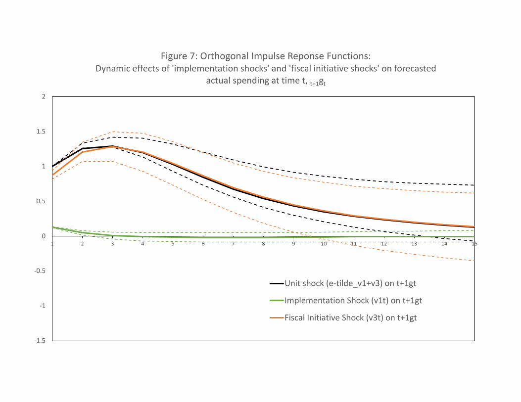
initiative shock identified in this way are plotted in Figure 6 and the impulse responses

associated with these two innovations are plotted in Figure 7, replicating the shape of the

response in Figure 5b and showing that this response is indeed driven primarily by the

initiative shock rather than the implementation shock. Figure 8 traces out the output ef-

fect too and Figure 9 translates these effects into the measure of the multiplier, calculated

as the ratio of the accumulated output effect divided by the accumulated spending effect

(and rescaled by the sample mean of output over spending to convert elasticities into

dollar units). This shows a total multiplier of effect of around 1.41 over the first six years

but rising to 1.72 ultimately. Moreover, the multiplier effect is still larger, reaching 1.79

at the long horizon, if we focus only on the effects of policy initiative shocks, showing that

the output effect of implementation shocks (whereby spending is higher than had been

originally planned) are actually negative. The total multiplier estimate is at the upper

end of the range of multiplier estimates for the U.S. that are reported in the literature14

14Ramey (2016) notes that these typically lie in the range [0.6, 1.5] although larger estimates are not

unusual. In the case of Australia, Li and Spencer (2015) develop a small open economy dynamic stochastic

[18]

but the finding that the output response to backward-looking policy reactions offsets that

of the more forward-looking policy initiatives is exactly as found in LMOS for the US and

illustrates the importance of being able to distinguish the effects of planned spending and

spending outcomes through the real-time dataset.

4 Concluding Comments

The Australian Real-Time Fiscal Database provides an invaluable source of information

on government spending, government receipts and its debt position, providing informa-

tion on plans as well as outcomes, as published in real time. The data is complex and

this paper provides an overview of the complexity, illustrating the nature of the defini-

tional changes and revisions that are embedded within it for example. But the data is

also extremely informative and necessary if decision-making is to be properly evaluated

taking into account the information available at the time. The empirical analysis of the

paper illustrates the point highlighting the predictability of the gaps between announced

plans and realised outcomes and showing the importance of distinguishing between policy

responses and policy initiatives in estimating the fiscal multiplier.

References

Bernoth, K., A. Hughes-Hallett, and J. Lewis (2008): “Did Fiscal Policy Makers

Know What They Were Doing? Reassessing Fiscal Policy with Real Time Data”,

CEPR Discussion Papers No. 6758.

Cimadomo, J. (2012), “Fiscal Policy in Real Time”, Scandinavian Journal of Eco-

nomics, Wiley Blackwell, vol. 114(2), 440-465, 06.

Croushore, D. (2011): “Frontiers of Real-Time Data Analysis,” Journal of Economic

Literature, 49, 72—100.

general equilibrium model and estimate the fiscal multiplier associated with the fiscal stimulus package

in the aftermath of the Global Financial Crisis. They also find estimates of the fiscal multiplier to be

relatively high with estimates of 0.9 on impact and 1.26 after one year.

[19]

Croushore, D. and C. I. Evans (2006), ”Data revisions and the identification of

monetary policy shocks”, Journal of Monetary Economics, Elsevier, vol. 53(6), pages

1135-1160, September.

Croushore, D., and T. Stark (2001): “A Real-Time Data Set for Macroeconomists”,

Journal of Econometrics, 105(1), 111—130.

Forni, L. and S. Momigliano (2005), “Cyclical Sensitivity of Fiscal Policies Based

on Real-time Data”, Applied Economics Quarterly, Volume 50, No. 3.

Galvao, A and M. Clements (2013), “Real-time Forecasting of Inflation and Output

Growth with Autoregressive Models in the Presence of Data Revisions”, Journal of

Applied Econometrics, 28: 458-477.

Garratt, A., K. Lee, E. Mise and K. Shields (2008), “Real Time Representations of

the Output Gap”, Review of Economics and Statistics, 90, 4, 792-804.

Garratt, A., K.C. Lee, E. Mise and K. Shields (2009), “Real Time Representations of

the UK Output Gap in the Presence of Model Uncertainty”, International Journal

of Forecasting, 25, 81-102.

Golinelli, R., and S. Momigliano (2006), “Real-Time Determinants of Fiscal Policies

in the Euro Area,” Journal of Policy Modeling, 28(9), 943-964.

Holm-Hadulla, F., S. Hauptmeier, and P. Rother (2012), “The Impact of Numerical

Expenditure Rules on Budgetary Discipline over the Cycle”, Applied Economics,

Vol. 44, Issue 25, 3287-3296.

Lee, K. C., J. Morley, K. Ong and K. Shields (2018), “Measuring the Fiscal Multi-

plier when Plans Take Time to Implement”, Working Paper.

Lee, K. C., J. Morley, K. Shields, and S. Tan (2015), Australian Fiscal Real-Time

Database: A Users Manual, available at

http://www.economics.unimelb.edu.au/RTAustralianMacroDatabase.

[20]

Li, S. M. and A. H. Spencer (2015), “Effectiveness of the Australian Fiscal Stimulus

Package: A DSGE Analysis”, The Economic Record, Vol. 92, Issue 296, 94-120.

Orphanides, A. and S. van Norden (2002), “The Unreliability of Output Gap Esti-

mates in Real Time”, Review of Economics and Statistics, 84, 4, 569-83.

Ramey, V. A. (2016), “Macroeconomic Shocks and Their Propagation”, Handbook

of Macroeconomics, 2, 71—162.

Ramey, V. and S. Zubairy (2018), “Government Spending Multipliers in Good Times

and in Bad: Evidence from U.S. Historical Data”, Journal of Political Economy,

126(2), 850—901.

[21]

-50000

0

50000

100000

150000

200000

250000

300000

350000

400000

450000

1947

-48

1952

-53

1957

-58

1962

-63

1967

-68

1972

-73

1977

-78

1982

-83

1987

-88

1992

-93

1997

-98

2002

-03

2007

-08

2012

-13

$ m

illio

nFigure 1a: Nominal Outlays, Investment and Transfers

OUTLAYS GOODS & SERVICESold GOODS & SERVICESnew CAPITALEXPold

CAPITALEXPnew TRANSFERSold TRANSFERSnew

-5%

0%

5%

10%

15%

20%

25%

30%

35%

1947

-48

1952

-53

1957

-58

1962

-63

1967

-68

1972

-73

1977

-78

1982

-83

1987

-88

1992

-93

1997

-98

2002

-03

2007

-08

2012

-13

% o

f GD

PFigure 1b: Nominal Outlays, Investment and Transfers (% of GDP)

OUTLAYS_Y GOODS & SERVICESold_Y GOODS & SERVICESnew_YCAPITALEXPold_Y CAPITALEXPnew_Y TRANSFERSold_YTRANSFERSnew_Y

0

50000

100000

150000

200000

250000

300000

350000

400000

1901

-02

1906

-07

1911

-12

1916

-17

1921

-22

1926

-27

1931

-32

1936

-37

1941

-42

1946

-47

1951

-52

1956

-57

1961

-62

1966

-67

1971

-72

1976

-77

1981

-82

1986

-87

1991

-92

1996

-97

2001

-02

2006

-07

2011

-12

$ m

illio

nFigure 1c: Nominal Receipts, Indirect and Direct Taxation

RECEIPTS INDIRECT TAX DIRECT TAX

0%

5%

10%

15%

20%

25%

30%

35%

1947

-48

1952

-53

1957

-58

1962

-63

1967

-68

1972

-73

1977

-78

1982

-83

1987

-88

1992

-93

1997

-98

2002

-03

2007

-08

2012

-13

% o

f GD

P

Figure 1d: Nominal Receipts, Indirect and Direct Taxation (% of GDP)

RECEIPTS_Y INDIRECT TAX_Y DIRECT TAX_Y

‐4000

‐2000

0

2000

4000

6000

8000

Vin

tage

1948

-49

Vin

tage

1951

-52

Vin

tage

1954

-55

Vin

tage

1957

-58

Vin

tage

1960

-61

Vin

tage

1963

-64

Vin

tage

1966

-67

Vin

tage

1969

-70

Vin

tage

1972

-73

Vin

tage

1975

-76

Vin

tage

1978

-79

Vin

tage

1981

-82

Vin

tage

1984

-85

Vin

tage

1987

-88

Vin

tage

1990

-91

Vin

tage

1993

-94

Vin

tage

1996

-97

Vin

tage

1999

-00

Vin

tage

2002

-03

Vin

tage

2005

-06

Vin

tage

2008

-09

Vin

tage

2011

-12

Vin

tage

2014

-15

$ m

illio

nsFigure 2a: Reported Surplus at 10 year Intervals from Vintages 1948-49 to 2015-16

alance 1948-49 alance 1958-59 alance 1968-69 alance 1978-79 alance 1988-89 alance 1998-99

‐5%

‐4%

‐3%

‐2%

‐1%

0%

1%

2%

3%

4%

5%V

inta

ge19

48-4

9

Vin

tage

1951

-52

Vin

tage

1954

-55

Vin

tage

1957

-58

Vin

tage

1960

-61

Vin

tage

1963

-64

Vin

tage

1966

-67

Vin

tage

1969

-70

Vin

tage

1972

-73

Vin

tage

1975

-76

Vin

tage

1978

-79

Vin

tage

1981

-82

Vin

tage

1984

-85

Vin

tage

1987

-88

Vin

tage

1990

-91

Vin

tage

1993

-94

Vin

tage

1996

-97

Vin

tage

1999

-00

Vin

tage

2002

-03

Vin

tage

2005

-06

Vin

tage

2008

-09

Vin

tage

2011

-12

Vin

tage

2014

-15

% o

f GD

PFigure 2b: Reported Surplus as a Percentage of GDP at 10 year Intervals from Vintages 1948-49

to 2015-16

Surplus Y: 1948-49 Surplus Y: 1958-59 Surplus Y: 1968-69Surplus Y: 1978-79 Surplus Y: 1988-89 Surplus Y: 1998-99

5

505

1005

1505

2005

2505

3005

3505

4005

4505

1946

1948

1950

1952

1954

1956

1958

1960

1962

1964

1966

1968

1970

1972

1974

1976

1978

1980

1982

1984

1986

1988

1990

1992

1994

1996

1998

2000

2002

2004

2006

2008

2010

2012

2014

$ m

illio

nsFigure 3a: Real Time Real Government Spending Releases for Australia: 1946 - 2015

tGt tGt-1 tGt-2

5

505

1005

1505

2005

2505

3005

3505

4005

1946

1948

1950

1952

1954

1956

1958

1960

1962

1964

1966

1968

1970

1972

1974

1976

1978

1980

1982

1984

1986

1988

1990

1992

1994

1996

1998

2000

2002

2004

2006

2008

2010

2012

2014

$m

illio

nsFigure 3b: Real Time Real Government Receipt Releases for Australia: 1946 - 2015

-1 -2

-800

-600

-400

-200

0

200

40019

46

1948

1950

1952

1954

1956

1958

1960

1962

1964

1966

1968

1970

1972

1974

1976

1978

1980

1982

1984

1986

1988

1990

1992

1994

1996

1998

2000

2002

2004

2006

2008

2010

2012

2014

$ m

illio

nsFigure 3c: Real Time Real Primary Balance Series for Australia: 1946 - 2015

tSPt tSPt-1 tSPt-2

0

0.05

0.1

0.15

0.2

0.25

0.3

0.35

0.4

1946

1948

1950

1952

1954

1956

1958

1960

1962

1964

1966

1968

1970

1972

1974

1976

1978

1980

1982

1984

1986

1988

1990

1992

1994

1996

1998

2000

2002

2004

2006

2008

2010

2012

2014

Figure 4: Ratios of Actual Spending to Output (tGt-1/tYt-1) and Actual Receipts to Output (t t-1/tYt-1)

tGt-1/tYt-1 t t-1/tYt-1

-1.5

-1

-0.5

0

0.5

1

1.5

2

1 2 3 4 5 6 7 8 9 10 11

Figure 5a: GIR of a unit tgt-1 ('e') shock

Unit tgt-1 shock (e) on tyt-1

Unit tgt-1 shock (e) on tgt

Unit tgt-1 shock (e) on tgt-1

-1.5

-1

-0.5

0

0.5

1

1.5

2

1 2 3 4 5 6 7 8 9 10 11

Figure 5b: GIR of a unit ('e-tilde') t+1gt shock

Unit t+1gt shock (e-tilde) on t+1gt

Unit t+1gt shock (e-tilde) on t+1gt+1

Unit t+1gt shock (etilde) on t+1yt

-6.0000

-4.0000

-2.0000

0.0000

2.0000

4.0000

6.0000

1957

1959

1961

1963

1965

1967

1969

1971

1973

1975

1977

1979

1981

1983

1985

1987

1989

1991

1993

1995

1997

1999

2001

2003

2005

2007

2009

2011

2013

2015

Figure 6: Implementation Shock (v1t) and Fiscal Shock (v3t) (with 1975, 2009 dummies)

Implementation Spending Shock Fiscal Spending Shock H. Holt (1966)J. McEwen (1967) J. Gorton (1968) W. McMahon (1971)G. Whitlam (1972) M. Fraser (1975) B. Hawke (1983)P. Keating (1991) J. Howard (1996) K. Rudd (2007)J. Gillard (2010) W. McMahon (1971) K. Rudd / T. Abbott (2013)M. Turnbull (2015)

-1.5

-1

-0.5

0

0.5

1

1.5

2

1 2 3 4 5 6 7 8 9 10 11 12 13 14 15

Figure 7: Orthogonal Impulse Reponse Functions: Dynamic effects of 'implementation shocks' and 'fiscal initiative shocks' on forecasted

actual spending at time t, t+1gt

Unit shock (e-tilde_v1+v3) on t+1gt

Implementation Shock (v1t) on t+1gt

Fiscal Initiative Shock (v3t) on t+1gt

0

0.4

0.8

1.2

1.6

1 2 3 4 5 6 7 8 9 10 11 12 13 14 15 16 17 18 19 20 21 22 23 24 25 26 27 28 29 30

Figure 8: Orthogonal Impulse Response Functions:Dynamic effects of 'implementation shocks' and 'fiscal initiative shocks' to forecasted

actual spending, t+1gt and forecasted actual output, t+1yt, at time t

Unit shock (e-tilde_v1+v3) on t+1gt

Unit shock (etilde_v1+v3) on t+1yt

0

0.2

0.4

0.6

0.8

1

1.2

1.4

1.6

1.8

2

1 2 3 4 5 6 30

Figure 9: Total Fiscal Multiplier and Fiscal Initiatives Multiplier

Total Fiscal Multiplier: (v1+v3) shock

Fiscal Initiatives Multiplier: v3 shock

Appendix

Table A1 Contents of t e Australian Real-Time Fiscal Dataset

No Name Notation in anual

First Vintage Date

Last Vintage Date

A Revenue 1 Receipts REV 1901-02 2015-16

2 Income Tax (Direct) DTAX 1901-02 2015-16 3 Expenditure Tax (Indirect) IDTAX 1901-02 2015-16 B Expenditure 4 Outlays OUT 1901-02 2015-16 5 Spending on Goods and Services GSEXP 1973-74 2015-16 6 ealt OUT EA 1946-47 2015-16 7 Education OUTEDU 1967-68 2015-16 8 Defence OUTDEF 1947-48 2015-16 9 Spending on Capital Goods CAPEXP 1973-74 2015-16

10 Transfers TPAY 1973-74 2015-16 11 elfare OUTSSEC 1946-47 2015-16 12 Pensions OUTPEN 1946-47 2015-16 13 Debt Interest Paid PDI 1962-63 2015-16 C Balance

14 Cas alance AL 1962-63 2015-16 15 Fiscal alance F AL 1999-00 2015-16 D Debt

16 Gross Debt GDE T 1925-26 2013-14 17 Public Debt PDE T 1912-13 2015-16 18 Net Debt NDE T 1994-95 2015-16 19 Commonwealt Interest Liability CO INTLIA 1932-33 1989-90 20 Total Interest Liability TOTINTLIA 1932-33 2015-16 21 Net Interest Outlays NIO 2002-03 2015-16 E Wealth

22 Net ort N ORT 1999-00 2015-16 23 Net Financial ort NF 2000-01 2015-16 24 Net Operating alance NO 1999-00 2015-16